





1. Introduction
1.1. Perturbation growth in turbulent flows
The well-known butterfly effect, introduced by Lorenz (Reference Lorenz1972), is commonly employed to explain the difficulties encountered when making weather predictions, an important example involving fluid turbulence. It was defined in more concrete mathematical terms by the same author (Lorenz Reference Lorenz1963) using a simple nonlinear model to study finite-amplitude convection with few degrees of freedom. Unstable chaotic solutions of these equations exhibit sensitivity to initial conditions and lie in a strange attractor, a term introduced by Ruelle & Takens (Reference Ruelle and Takens1971). This was then shown to be the case for turbulent (unstable) solutions of the Navier–Stokes equations by Deissler (Reference Deissler1986). The time evolution (growth) of a small perturbation applied to turbulent flows has been studied well (Lorenz Reference Lorenz1969; Leith & Kraichnan Reference Leith and Kraichnan1972; Boffetta et al. Reference Boffetta, Celani, Crisanti and Vulpiani1997; Berera & Ho Reference Berera and Ho2018). In the context of infinitesimal perturbations, it is well established that, after transient effects have subsided, these perturbations evolve approximately and asymptotically in an exponential manner, governed by the largest Lyapunov exponent (Ruelle Reference Ruelle1981; Eckmann & Ruelle Reference Eckmann and Ruelle1985). As the size of these perturbations becomes finite, an algebraic growth of the perturbation in time has been observed to follow (Boffetta & Musacchio Reference Boffetta and Musacchio2017). In homogeneous and isotropic turbulence (HIT), during this phase, a self-similar evolution of the small perturbation has been observed, involving an inverse cascade through which the perturbation propagates from small to large scales (Lorenz Reference Lorenz1969; Leith & Kraichnan Reference Leith and Kraichnan1972; Boffetta & Musacchio Reference Boffetta and Musacchio2017; Vela-Martín Reference Vela-Martín2024, Reference Vela-Martín2025).
Efforts have also been made to elucidate the process of perturbation growth in terms of the physical mechanisms involved in turbulence. Ruelle (Reference Ruelle1979) proposed that the largest Lyapunov exponent scales inversely to the well-known Kolmogorov time scale and Crisanti et al. (Reference Crisanti, Jensen, Vulpiani, Paladin and Moro1993) introduced a small correction to this model based on intermittency. However, emerging observations (Boffetta & Musacchio Reference Boffetta and Musacchio2017; Mohan, Fitzsimmons & Moser Reference Mohan, Fitzsimmons and Moser2017; Ge, Rolland & Vassilicos Reference Ge, Rolland and Vassilicos2023) do not support the early scaling model and instead indicate that the largest Lyapunov exponent may scale with a sub-Kolmogorov time scale. Furthermore, recently, the mechanisms for the growth of the perturbation have been proposed in terms of structures of the flow. For example, in HIT, Mohan et al. (Reference Mohan, Fitzsimmons and Moser2017) identified that the main instabilities act on the smallest eddies and suggested pairing instabilities of corotating vortices as one of the possible mechanisms. In another study, Ge et al. (Reference Ge, Rolland and Vassilicos2023) used the energy budget equation for a small perturbation and concluded that the growth of the perturbation is dominated by compression events of the strain rate, whilst its stretching events decrease the uncertainty.
1.2. Near-wall turbulence
Near-wall turbulence is of fundamental importance in a wide range of engineering disciplines, including aeronautical, mechanical, chemical and environmental engineering. Unlike the case of HIT, considered by most of the previously listed studies, near-wall turbulence is highly anisotropic and involves complex nonlinear and non-local interactions between energy-containing coherent structures, the size of which varies from the viscous inner to the large outer length scales. It has been understood that the predominant structures of the near-wall turbulence are elongated spanwise-alternating high- and low-speed fluid areas, called streaks (Kline et al. Reference Kline, Reynolds, Schraub and Runstadler1967; Kim, Kline & Reynolds Reference Kim, Kline and Reynolds1971; Smith & Metzler Reference Smith and Metzler1983), and quasi-streamwise vortices, which play an important role in transport of fluid momentum in the wall-normal direction (Blackwelder & Eckelmann Reference Blackwelder and Eckelmann1979; Kim, Moin & Moser Reference Kim, Moin and Moser1987). The interactions between the two are known to be crucial aspects of the generation of near-wall turbulence. In particular, using the minimal flow unit approach (Jiménez & Moin Reference Jiménez and Moin1991), Hamilton, Kim & Waleffe (Reference Hamilton, Kim and Waleffe1995) proposed the self-sustaining process of near-wall turbulence, a theoretical and mechanistic description of the dynamical interplay between streaks and quasi-streamwise vortices. The amplification of streaks from quasi-streamwise vortices has been well understood in terms of the so-called lift-up effect. This process, associated with the non-normality of the linearised Navier–Stokes operator, enables streamwise vortices to displace low-momentum fluid away from the wall and high-momentum fluid towards the wall, while transferring the energy of mean shear to the streaks (Landahl Reference Landahl1990; Butler & Farrell Reference Butler and Farrell1993; Chernyshenko & Baig Reference Chernyshenko and Baig2005; del Álamo & Jiménez Reference del Álamo and Jiménez2006; Pujals et al. Reference Pujals, García-Villalba, Cossu and Depardon2009; Hwang & Cossu Reference Hwang and Cossu2010a , Reference Hwang and Cossub ). The amplified streaks undergo an instability and/or transient growth (Hamilton et al. Reference Hamilton, Kim and Waleffe1995; Waleffe Reference Waleffe1997; Schoppa & Hussain Reference Schoppa and Hussain2002; Cassinelli, Giovanetti & Hwang Reference Cassinelli, Giovanetti and Hwang2017; Lozano-Durán et al. Reference Lozano-Durán, Constantinou, Nikolaidis and Karp2021; Markeviciute & Kerswell Reference Markeviciute and Kerswell2024; Oxley & Kerswell Reference Oxley and Kerswell2025) and the subsequent nonlinear interactions regenerate the vortices.
The growth of small perturbations for near-wall turbulence has also been studied, especially the early exponential growth dictated by the leading Lyapunov exponent. Nikitin (Reference Nikitin2009, Reference Nikitin2018) and Nikitin & Pivovarov (Reference Nikitin and Pivovarov2018) carried out studies in a circular pipe and a plane channel for a range of Reynolds numbers. It was shown that the leading Lyapunov vector is concentrated mainly in the buffer layer and emerges in the form of spots localised both in time and space. He also attributed the perturbation growth to the streamwise inhomogeneity of the base flow, as well as to the presence of transversal motion in it. Inubushi, Takehiro & Yamada (Reference Inubushi, Takehiro and Yamada2015) computed the covariant Lyapunov vectors in plane Couette flow using the minimal flow unit of Hamilton et al. (Reference Hamilton, Kim and Waleffe1995). They found that the positive Lyapunov exponents are mainly associated with the perturbation growth during the streak breakdown phase (i.e. highly disorganised flow state), consistent with the observation by Nikitin (Reference Nikitin2018).
1.3. Scope of this study
As it has been previously shown, in HIT, small perturbations propagate from the smallest scales of the flow to the largest scales through an inverse cascade. However, in wall turbulence, the flow is highly anisotropic and the related coherent structures play a key role in momentum and energy transfer of small perturbations. The objective of this work is to provide a characterisation and a deeper understanding of the growth of small perturbations in wall turbulence over the full time horizon and, specifically, to analyse the correlation of this growth to the dynamics of the fundamental coherent structures, as described by the self-sustaining process. The latter has been considered as the most fundamental unit in wall turbulence for the last two decades. In particular, the turbulent channel DNS studies of Hwang (Reference Hwang2015) and Hwang & Bengana (Reference Hwang and Bengana2016) have shown the presence of the self-sustaining process at the different scales of wall turbulence (from the near-wall to the outer layer); hence, a characterisation of the contributions from the self-sustaining process to perturbation growth in wall turbulence is key to understand said growth. To this end, in the present study, we choose to isolate the fundamental structures of wall turbulence, making use of the minimal flow unit in plane Couette flow (Jiménez & Moin Reference Jiménez and Moin1991; Hamilton et al. Reference Hamilton, Kim and Waleffe1995), where the dynamical interactions between streaks and quasi-streamwise vortices through the self-sustaining process can be simulated in an isolated manner. Using a set of equations that quantify the contributions to the energy of perturbations from each element of the coherent structures, we examine the evolution of small perturbations over a long time interval and their propagation through the coherent structures.
This paper is organised as follows. The problem formulation analysed in this work and the methodology employed to carry out said analysis are described in § 2. The results obtained from the DNS are analysed in § 3, where the key mechanisms contributing to the growth of the perturbation are identified. A discussion of the findings and the theory proposed for the evolution of the perturbation beyond the Lyapunov time is carried out in § 4. Finally, a summary of the key findings and some concluding remarks are presented in § 5.
2. Problem formulation
We consider turbulent Couette flow, where a fluid is bounded by two walls moving in opposite directions with a streamwise velocity of $\pm U_w$
. The two walls are separated by a distance of
$\pm U_w$
. The two walls are separated by a distance of $2h$
. The kinematic viscosity is denoted by
$2h$
. The kinematic viscosity is denoted by $\nu$
and the Reynolds number is defined as
$\nu$
and the Reynolds number is defined as $Re=U_wh/\nu$
. All variables are dimensionless using
$Re=U_wh/\nu$
. All variables are dimensionless using $h$
and
$h$
and $U_w$
as length and velocity scales. The non-dimensional streamwise, wall-normal and spanwise coordinates are denoted by
$U_w$
as length and velocity scales. The non-dimensional streamwise, wall-normal and spanwise coordinates are denoted by $(x,y,z)$
, and the domain of interest is defined as
$(x,y,z)$
, and the domain of interest is defined as $(x,y,z)\in [0,L_x] \times [-1, 1] \times [0,L_z]$
. Periodic boundary conditions are imposed in the wall-parallel directions, and the no-slip condition is enforced in the top and bottom walls. Following Hamilton et al. (Reference Hamilton, Kim and Waleffe1995), the wall-parallel size of the domain is set with
$(x,y,z)\in [0,L_x] \times [-1, 1] \times [0,L_z]$
. Periodic boundary conditions are imposed in the wall-parallel directions, and the no-slip condition is enforced in the top and bottom walls. Following Hamilton et al. (Reference Hamilton, Kim and Waleffe1995), the wall-parallel size of the domain is set with $L_x = 1.75 \pi$
and
$L_x = 1.75 \pi$
and $L_z = 1.2 \pi$
. The Reynolds number is set to be
$L_z = 1.2 \pi$
. The Reynolds number is set to be $Re=400$
.
$Re=400$
.
2.1. Equations of motion
We start by introducing a decomposition of an instantaneous velocity field, $\boldsymbol{u}(\boldsymbol{x},t)$
, as follows:
$\boldsymbol{u}(\boldsymbol{x},t)$
, as follows:
 \begin{equation} \boldsymbol{u}(\boldsymbol{x},t) = \boldsymbol{U}(\boldsymbol{x},t) + \boldsymbol{u'}(\boldsymbol{x},t), \end{equation}
where $\boldsymbol{U}(\boldsymbol{x},t)(=(U(y,t),0,W(y,t)))$
and
$\boldsymbol{U}(\boldsymbol{x},t)(=(U(y,t),0,W(y,t)))$
and $\boldsymbol{u'}(\boldsymbol{x},t)$
represent the velocity averaged over
$\boldsymbol{u'}(\boldsymbol{x},t)$
represent the velocity averaged over $x$
and
$x$
and $z$
and the fluctuating velocity, respectively. Further, following Doohan et al. (Reference Doohan, Bengana, Yang, Willis and Hwang2022), where detailed interaction energetics of the self-sustaining process are studied at different length scales, we decompose the fluctuating velocity into
$z$
and the fluctuating velocity, respectively. Further, following Doohan et al. (Reference Doohan, Bengana, Yang, Willis and Hwang2022), where detailed interaction energetics of the self-sustaining process are studied at different length scales, we decompose the fluctuating velocity into
 \begin{equation} \boldsymbol{u'}(\boldsymbol{x},t) = \boldsymbol{u}_1( y,z,t) + \boldsymbol{u}_2(\boldsymbol{x},t), \end{equation}
with $\boldsymbol{u}_1(y,z,t) = \langle \boldsymbol{u'}(\boldsymbol{x},t)\rangle _{x}$
, where
$\boldsymbol{u}_1(y,z,t) = \langle \boldsymbol{u'}(\boldsymbol{x},t)\rangle _{x}$
, where $\langle \boldsymbol{\cdot }\rangle _{x}$
denotes the average in the
$\langle \boldsymbol{\cdot }\rangle _{x}$
denotes the average in the $x$
-direction. We note that the fluctuating flow averaged in the streamwise direction,
$x$
-direction. We note that the fluctuating flow averaged in the streamwise direction, $\boldsymbol{u}_1$
, characterises the streamwise elongated flow structures (streaks), while the rest of the fluctuating velocity represents the streamwise varying structures (meandering motions of streaks due to streak instability or transient growth and quasi-streamwise vortices). The pressure can be decomposed similarly, i.e.
$\boldsymbol{u}_1$
, characterises the streamwise elongated flow structures (streaks), while the rest of the fluctuating velocity represents the streamwise varying structures (meandering motions of streaks due to streak instability or transient growth and quasi-streamwise vortices). The pressure can be decomposed similarly, i.e. $P(\boldsymbol{x},t) = P + p_1+p_2$
. The resulting dimensionless equations of motion are given by
$P(\boldsymbol{x},t) = P + p_1+p_2$
. The resulting dimensionless equations of motion are given by
 \begin{align} \frac {\partial \boldsymbol{U}}{\partial t} + (\boldsymbol{U} \boldsymbol{\cdot }\boldsymbol{\nabla }) \boldsymbol{U} + \langle (\boldsymbol{u'} \boldsymbol{\cdot }\boldsymbol{\nabla }) \boldsymbol{u'} \rangle _{x,z} & = -\boldsymbol{\nabla }P + \frac {1}{Re}{\nabla} ^2 \boldsymbol{U}, \end{align}
 \begin{align} \frac {\partial \boldsymbol{u}_1}{\partial t} + (\boldsymbol{u}_1 \boldsymbol{\cdot }\boldsymbol{\nabla }) \boldsymbol{U} + (\boldsymbol{U} \boldsymbol{\cdot }\boldsymbol{\nabla }) \boldsymbol{u}_1 + (\boldsymbol{u}_1 \boldsymbol{\cdot }\boldsymbol{\nabla }) \boldsymbol{u}_1 &+ \langle (\boldsymbol{u}_2 \boldsymbol{\cdot }\boldsymbol{\nabla }) \boldsymbol{u}_2 \rangle _{x} - \langle (\boldsymbol{u'} \boldsymbol{\cdot }\boldsymbol{\nabla }) \boldsymbol{u'} \rangle _{x,z}\nonumber\\ & = -\boldsymbol{\nabla }p_1 + \frac {1}{Re} {\nabla} ^2 \boldsymbol{u}_1, \end{align}
 \begin{align} \frac {\partial \boldsymbol{u}_2}{\partial t} + [(\boldsymbol{U} + \boldsymbol{u}_1) \boldsymbol{\cdot }\boldsymbol{\nabla }] \boldsymbol{u}_2 + (\boldsymbol{u}_2 \boldsymbol{\cdot }\boldsymbol{\nabla }) & [\boldsymbol{U} + \boldsymbol{u}_1] + (\boldsymbol{u}_2 \boldsymbol{\cdot }\boldsymbol{\nabla }) \boldsymbol{u}_2 - \langle (\boldsymbol{u}_2 \boldsymbol{\cdot }\boldsymbol{\nabla }) \boldsymbol{u}_2\rangle _{x}\nonumber\\ & = -\boldsymbol{\nabla }p_2 + \frac {1}{Re} {\nabla} ^2 \boldsymbol{u}_2, \end{align}
where $\langle \boldsymbol{\cdot }\rangle _{x,z}$
denotes the average in the
$\langle \boldsymbol{\cdot }\rangle _{x,z}$
denotes the average in the $x$
- and
$x$
- and $z$
-directions. We emphasise that the velocity decomposition introduced here is intended specifically for minimal flow units. In such domains, the restriction on admissible streamwise length scales ensures that the streamwise averaged component
$z$
-directions. We emphasise that the velocity decomposition introduced here is intended specifically for minimal flow units. In such domains, the restriction on admissible streamwise length scales ensures that the streamwise averaged component $\boldsymbol{u}_1$
provides a meaningful characterisation of streak dynamics, while the remaining component
$\boldsymbol{u}_1$
provides a meaningful characterisation of streak dynamics, while the remaining component $\boldsymbol{u}_2$
captures their streamwise meandering motions caused by the instability or transient growth. In very large domains, where streaks of widely varying streamwise extent and multiple meandering or instability wavelengths coexist simultaneously, this decomposition and the associated global diagnostics derived from it are not, in general, expected to provide a complete description of the dynamics.
$\boldsymbol{u}_2$
captures their streamwise meandering motions caused by the instability or transient growth. In very large domains, where streaks of widely varying streamwise extent and multiple meandering or instability wavelengths coexist simultaneously, this decomposition and the associated global diagnostics derived from it are not, in general, expected to provide a complete description of the dynamics.
2.2. Perturbation energy budget
We now consider a perturbation applied to a given reference flow field from a statistically steady turbulent state:
 \begin{equation} \Delta \boldsymbol{u} = \boldsymbol{u}^{(2)} - \boldsymbol{u}^{(1)}, \end{equation}
where $\boldsymbol{u}^{(1)}$
is the ‘unperturbed’ reference flow field and
$\boldsymbol{u}^{(1)}$
is the ‘unperturbed’ reference flow field and $\boldsymbol{u}^{(2)}$
is the corresponding perturbed one with
$\boldsymbol{u}^{(2)}$
is the corresponding perturbed one with $\Delta \boldsymbol{u}$
. Using (2.6), and the equations of motion given in (2.3), (2.4) and (2.5), the equations for each componet of the perturbation field (i.e.
$\Delta \boldsymbol{u}$
. Using (2.6), and the equations of motion given in (2.3), (2.4) and (2.5), the equations for each componet of the perturbation field (i.e. $\Delta \boldsymbol{U}$
,
$\Delta \boldsymbol{U}$
, $\Delta \boldsymbol{u}_1$
and
$\Delta \boldsymbol{u}_1$
and $\Delta \boldsymbol{u}_2$
) are obtained, as documented in Appendix A: see (A1), (A2) and (A3). Using the corresponding energy equations for each perturbation field (see (A4), (A5) and (A6) in Appendix A), the time evolution of the volume-averaged perturbation energy for
$\Delta \boldsymbol{u}_2$
) are obtained, as documented in Appendix A: see (A1), (A2) and (A3). Using the corresponding energy equations for each perturbation field (see (A4), (A5) and (A6) in Appendix A), the time evolution of the volume-averaged perturbation energy for $\Delta \boldsymbol{U}$
,
$\Delta \boldsymbol{U}$
, $\Delta \boldsymbol{u}_1$
and
$\Delta \boldsymbol{u}_1$
and $\Delta \boldsymbol{u}_2$
is given by
$\Delta \boldsymbol{u}_2$
is given by
 \begin{align} \frac {\partial E_{\Delta \boldsymbol{U}}}{\partial t} &= P_{\Delta \boldsymbol{U}}+T_{\Delta \boldsymbol{U}}-\epsilon _{\Delta \boldsymbol{U}}, \end{align}
 \begin{align} \frac {\partial E_{\Delta \boldsymbol{u}_1}}{\partial t} &= P_{\Delta \boldsymbol{u}_1}+T_{\Delta \boldsymbol{u}_1}-\epsilon _{\Delta \boldsymbol{u}_1}, \end{align}
 \begin{align} \frac {\partial E_{\Delta \boldsymbol{u}_2}}{\partial t} &= P_{\Delta \boldsymbol{u}_2}+T_{\Delta \boldsymbol{u}_2}-\epsilon _{\Delta \boldsymbol{u}_2}, \end{align}
where
 \begin{equation} E_{\Delta \boldsymbol{U}}= \frac {1}{2}\langle \Delta \boldsymbol{U} \boldsymbol{\cdot }\Delta \boldsymbol{U} \rangle , \quad E_{\Delta \boldsymbol{u}_1}= \frac {1}{2}\langle \Delta \boldsymbol{u}_1 \boldsymbol{\cdot }\Delta \boldsymbol{u}_1 \rangle \quad \text{and} \quad E_{\Delta \boldsymbol{u}_2}= \frac {1}{2}\langle \Delta \boldsymbol{u}_2 \boldsymbol{\cdot }\Delta \boldsymbol{u}_2 \rangle \end{equation}
are the volume-averaged kinetic energies of the three flow components ( $\langle \boldsymbol{\cdot }\rangle \equiv 1/V \int _\varOmega (\boldsymbol{\cdot })\, \textrm {d}V,$
where
$\langle \boldsymbol{\cdot }\rangle \equiv 1/V \int _\varOmega (\boldsymbol{\cdot })\, \textrm {d}V,$
where $\varOmega$
is the given flow domain and
$\varOmega$
is the given flow domain and $V$
is its volume). Here, the three production terms are written as
$V$
is its volume). Here, the three production terms are written as
 \begin{align} P_{\Delta \boldsymbol{U}} = & -\biggl (\left \langle \Delta \boldsymbol{U} \boldsymbol{\cdot }(\Delta \boldsymbol{U} \boldsymbol{\cdot }\boldsymbol{\nabla }) \boldsymbol{U}^{(1)} \right \rangle +\left \langle \Delta \boldsymbol{U} \boldsymbol{\cdot }(\Delta \boldsymbol{u}_1 \boldsymbol{\cdot }\boldsymbol{\nabla }) \boldsymbol{u}_1^{(1)} \right \rangle \nonumber\\ &+ \left \langle \Delta \boldsymbol{U} \boldsymbol{\cdot }(\Delta \boldsymbol{u}_2 \boldsymbol{\cdot }\boldsymbol{\nabla }) \boldsymbol{u}_2^{(1)} \right \rangle \biggr ), \end{align}
 \begin{align} P_{\Delta \boldsymbol{u}_1} = & -\biggl ( \left \langle \Delta \boldsymbol{u}_1 \boldsymbol{\cdot }(\Delta \boldsymbol{u}_1 \boldsymbol{\cdot }\boldsymbol{\nabla })\boldsymbol{U}^{(1)} \right \rangle + \left \langle \Delta \boldsymbol{u}_1 \boldsymbol{\cdot }(\Delta \boldsymbol{U} \boldsymbol{\cdot }\boldsymbol{\nabla })\boldsymbol{u}_1^{(1)} \right \rangle \nonumber\\ &+\left \langle \Delta \boldsymbol{u}_1 \boldsymbol{\cdot }(\Delta \boldsymbol{u}_1 \boldsymbol{\cdot }\boldsymbol{\nabla })\boldsymbol{u}_1^{(1)} \right \rangle + \left \langle \Delta \boldsymbol{u}_1 \boldsymbol{\cdot }(\Delta \boldsymbol{u}_2 \boldsymbol{\cdot }\boldsymbol{\nabla })\boldsymbol{u}_2^{(1)} \right \rangle \biggr ), \end{align}
 \begin{align} P_{\Delta \boldsymbol{u}_2}= & -\biggl ( \left \langle \Delta \boldsymbol{u}_2 \boldsymbol{\cdot }(\Delta \boldsymbol{U} \boldsymbol{\cdot }\boldsymbol{\nabla })\boldsymbol{u}_2^{(1)} \right \rangle + \left \langle \Delta \boldsymbol{u}_2 \boldsymbol{\cdot }(\Delta \boldsymbol{u}_1 \boldsymbol{\cdot }\boldsymbol{\nabla })\boldsymbol{u}_2^{(1)} \right \rangle \nonumber\\ &+\left \langle \Delta \boldsymbol{u}_2 \boldsymbol{\cdot }(\Delta \boldsymbol{u}_2 \boldsymbol{\cdot }\boldsymbol{\nabla })\boldsymbol{U}^{(1)} \right \rangle + \left \langle \Delta \boldsymbol{u}_2 \boldsymbol{\cdot }(\Delta \boldsymbol{u}_2 \boldsymbol{\cdot }\boldsymbol{\nabla })\boldsymbol{u}_1^{(1)} \right \rangle \nonumber\\ &+ \left \langle \Delta \boldsymbol{u}_2 \boldsymbol{\cdot }(\Delta \boldsymbol{u}_2 \boldsymbol{\cdot }\boldsymbol{\nabla })\boldsymbol{u}_2^{(1)} \right \rangle \biggr ). \end{align}
Similarly, the transport terms are given by
 \begin{align} T_{\Delta \boldsymbol{U}}= & -\biggl ( \left \langle \Delta \boldsymbol{U} \boldsymbol{\cdot }(\boldsymbol{u}_1^{(1)} \boldsymbol{\cdot }\boldsymbol{\nabla })\Delta \boldsymbol{u}_1 \right \rangle + \left \langle \Delta \boldsymbol{U} \boldsymbol{\cdot }(\Delta \boldsymbol{u}_1 \boldsymbol{\cdot }\boldsymbol{\nabla })\Delta \boldsymbol{u}_1 \right \rangle \nonumber\\ &+ \left \langle \Delta \boldsymbol{U} \boldsymbol{\cdot }(\boldsymbol{u}_2^{(1)} \boldsymbol{\cdot }\boldsymbol{\nabla })\Delta \boldsymbol{u}_2 \right \rangle + \left \langle \Delta \boldsymbol{U} \boldsymbol{\cdot }(\Delta \boldsymbol{u}_2 \boldsymbol{\cdot }\boldsymbol{\nabla })\Delta \boldsymbol{u}_2 \right \rangle \biggr ), \end{align}
 \begin{align} T_{\Delta \boldsymbol{u}_1}= & -\biggl ( \left \langle \Delta \boldsymbol{u}_1 \boldsymbol{\cdot }(\boldsymbol{u}_1^{(1)} \boldsymbol{\cdot }\boldsymbol{\nabla })\Delta \boldsymbol{U} \right \rangle + \left \langle \Delta \boldsymbol{u}_1 \boldsymbol{\cdot }(\Delta \boldsymbol{u}_1 \boldsymbol{\cdot }\boldsymbol{\nabla })\Delta \boldsymbol{U} \right \rangle \nonumber\\ &+\left \langle \Delta \boldsymbol{u}_1 \boldsymbol{\cdot }(\boldsymbol{u}_2^{(1)} \boldsymbol{\cdot }\boldsymbol{\nabla })\Delta \boldsymbol{u}_2 \right \rangle + \left \langle \Delta \boldsymbol{u}_1 \boldsymbol{\cdot }(\Delta \boldsymbol{u}_2 \boldsymbol{\cdot }\boldsymbol{\nabla })\Delta \boldsymbol{u}_2 \right \rangle \biggr ), \end{align}
 \begin{align} T_{\Delta \boldsymbol{u}_2}= &-\biggl ( \left \langle \Delta \boldsymbol{u}_2 \boldsymbol{\cdot }(\boldsymbol{u}_2^{(1)} \boldsymbol{\cdot }\boldsymbol{\nabla })\Delta \boldsymbol{U} \right \rangle + \left \langle \Delta \boldsymbol{u}_2 \boldsymbol{\cdot }(\Delta \boldsymbol{u}_2 \boldsymbol{\cdot }\boldsymbol{\nabla })\Delta \boldsymbol{U} \right \rangle \nonumber\\ &+ \left \langle \Delta \boldsymbol{u}_2 \boldsymbol{\cdot }(\boldsymbol{u}_2^{(1)} \boldsymbol{\cdot }\boldsymbol{\nabla })\Delta \boldsymbol{u}_1 \right \rangle + \left \langle \Delta \boldsymbol{u}_2 \boldsymbol{\cdot }(\Delta \boldsymbol{u}_2 \boldsymbol{\cdot }\boldsymbol{\nabla })\Delta \boldsymbol{u}_1 \right \rangle \biggr ). \end{align}
Finally, the dissipation and diffusion terms are
 \begin{equation} \begin{aligned} \epsilon _{\Delta \boldsymbol{U}} &= -\left \langle \frac {1}{Re} \Delta \boldsymbol{U} \boldsymbol{\cdot }{\nabla} ^2 \Delta \boldsymbol{U} \right \rangle , \quad\; \epsilon _{\Delta \boldsymbol{u}_1} = -\left \langle \frac {1}{Re} \Delta \boldsymbol{u}_1 \boldsymbol{\cdot }{\nabla} ^2 \Delta \boldsymbol{u}_1 \right \rangle , \quad\; \nonumber\\ \epsilon _{\Delta \boldsymbol{u}_2} &= -\left \langle \frac {1}{Re} \Delta \boldsymbol{u}_2 \boldsymbol{\cdot }{\nabla} ^2 \Delta \boldsymbol{u}_2 \right \rangle . \end{aligned} \end{equation}
It can be seen that (2.7), (2.8) and (2.9) are made up of a term expressing the time evolution of the energy, a set of production terms, a set of transport terms and a viscous term, respectively. In general, the production terms contribute to the growth of the perturbation energy and the viscous terms take energy away from the perturbation energy. The transport terms do not add or subtract any energy to the ‘total’ energy budget (see (2.18)), as they cancel each other when added together, but rather redistribute energy amongst the three different components ( $\Delta \boldsymbol{U}$
,
$\Delta \boldsymbol{U}$
, $\Delta \boldsymbol{u}_1$
and
$\Delta \boldsymbol{u}_1$
and $\Delta \boldsymbol{u}_2$
). Therefore, in this work, we use the term ‘transport’ in the sense that they add/subtract energy to one component and subtract/add it to another, without affecting the total budget. This is indeed the behaviour observed for these terms and will be analysed in § 3.
$\Delta \boldsymbol{u}_2$
). Therefore, in this work, we use the term ‘transport’ in the sense that they add/subtract energy to one component and subtract/add it to another, without affecting the total budget. This is indeed the behaviour observed for these terms and will be analysed in § 3.
When adding (2.7), (2.8) and (2.9), the transport terms do not add or subtract energy from the system as a whole and cancel with each other. Therefore, adding the three equations leads to the following perturbation energy balance equation:
 \begin{equation} \frac {\mathrm{d} E_\Delta }{\mathrm{d}t} = P_\Delta - \epsilon _\Delta \end{equation}
with
 \begin{equation} E_\Delta = \frac {1}{2}\langle \Delta \boldsymbol{u} \boldsymbol{\cdot }\Delta \boldsymbol{u} \rangle , \end{equation}
where production and dissipation, $P_\Delta$
and
$P_\Delta$
and $\epsilon _\Delta$
, are defined as
$\epsilon _\Delta$
, are defined as
 \begin{equation} P_\Delta = -\left \langle \Delta \boldsymbol{u} \boldsymbol{\cdot }(\Delta \boldsymbol{u} \boldsymbol{\cdot }\boldsymbol{\nabla }) \boldsymbol{u}^{(1)} \right \rangle , \quad \epsilon _\Delta = \frac {2}{Re}\langle s_{\Delta ,ij}s_{\Delta ,ij}\rangle \end{equation}
with
 \begin{equation} s_{\Delta ,ij} = \frac {1}{2} \left ( \frac {\partial \Delta u_i}{\partial x_j} + \frac {\partial \Delta u_j}{\partial x_i} \right ). \end{equation}
Here, the dissipation term is written in tensor notation for simplicity.
2.3. Numerical set-ups
Direct numerical simulations in the present study are carried out using the open-source code Channelflow 2.0 (
https://www.channelflow.ch/
), a software to analyse incompressible channel flows. The solver is spectral with the Fourier–Galerkin method used in the wall-parallel dimensions and the Chebyshev-tau method used in the wall-normal dimension. In time, the Navier–Stokes equations are integrated using a third-order semi-implicit backward differentiation scheme. The domain is discretised into a grid of $16 \times 33 \times 16$
cells in
$16 \times 33 \times 16$
cells in $x$
,
$x$
, $y$
and
$y$
and $z$
, respectively (after dealiasing), the same discretisation as the one used by Hamilton et al. (Reference Hamilton, Kim and Waleffe1995). The friction Reynolds number is obtained as
$z$
, respectively (after dealiasing), the same discretisation as the one used by Hamilton et al. (Reference Hamilton, Kim and Waleffe1995). The friction Reynolds number is obtained as $Re_\tau$
= 34 from the simulations, where
$Re_\tau$
= 34 from the simulations, where $Re_\tau =u_\tau h/\nu$
and
$Re_\tau =u_\tau h/\nu$
and $u_\tau$
is the friction velocity.
$u_\tau$
is the friction velocity.
3. Time evolution of a perturbation over the full time horizon
To study the time evolution of small perturbations, we start by generating an initial (reference) turbulent velocity field, $\boldsymbol{u}^{(1)}$
, to which we subsequently add a small perturbation of zero divergence and no-slip boundary conditions. This results in a perturbed velocity field
$\boldsymbol{u}^{(1)}$
, to which we subsequently add a small perturbation of zero divergence and no-slip boundary conditions. This results in a perturbed velocity field $\boldsymbol{u}^{(2)}$
. The form (in terms of the distribution along different scales) of each perturbation is random. To verify this has no effect in the evolution of the perturbation, we carried out a short validation study, where each component of the reference field (
$\boldsymbol{u}^{(2)}$
. The form (in terms of the distribution along different scales) of each perturbation is random. To verify this has no effect in the evolution of the perturbation, we carried out a short validation study, where each component of the reference field ( $\boldsymbol{U}^{(1)}$
,
$\boldsymbol{U}^{(1)}$
, $\boldsymbol{u}_1^{(1)}$
and
$\boldsymbol{u}_1^{(1)}$
and $\boldsymbol{u}_2^{(1)}$
) was perturbed independently. The results can be seen in figure 12 in Appendix C. Once the transient response dies out, the three cases evolve in the same qualitative manner and we therefore conclude there are no direct effects from this.
$\boldsymbol{u}_2^{(1)}$
) was perturbed independently. The results can be seen in figure 12 in Appendix C. Once the transient response dies out, the three cases evolve in the same qualitative manner and we therefore conclude there are no direct effects from this.
Both perturbed and unperturbed fields are then evolved in time, and, by subtracting one from the other, we obtain the time evolution of the perturbation. The results presented, unless stated, are ensemble-averaged using 65 different realisations to filter out unpredictable local flow patterns. The time evolution of the perturbation energy is shown in figure 1, where the initial energy of the perturbation is chosen to be $ E_\Delta (0)=10^{-5}$
. We note that perturbations with different values of the initial perturbation energy (
$ E_\Delta (0)=10^{-5}$
. We note that perturbations with different values of the initial perturbation energy ( $ E_\Delta (0)=10^{-4}, 10^{-6}$
) were tested, but there were no qualitative differences to figure 1 in the time evolution of
$ E_\Delta (0)=10^{-4}, 10^{-6}$
) were tested, but there were no qualitative differences to figure 1 in the time evolution of $ E_\Delta (t)$
.
$ E_\Delta (t)$
.
Time evolution of perturbation energy shown in lin–log axes. The figure is divided into three sections, from left to right: transient response, short-term response corresponding to the exponential evolution and long-term response. In the asymptotic evolution section, an estimate fitting for the exponential growth is shown. Note, the long-term response analysis will cover up to $t=5000$
, but the period up to
$t=5000$
, but the period up to $t=1000$
is shown for visualisation purposes.
$t=1000$
is shown for visualisation purposes.

The evolution of the perturbation energy shows the expected trends. There is a short initial transient response where there is a decrease of perturbation energy followed by the exponential regime and the saturated period. From the figure and the fitted line, the leading Lyapunov exponent is estimated by using
 \begin{equation} \lambda = \lim _{t\rightarrow \infty }\frac {1}{2t}\log \left ( \frac { E_\Delta (t) }{E_\Delta (0)} \right ). \end{equation}
In this case, the leading Lyapunov exponent is found to be $\lambda \approx 0.025$
. This value is in good agreement with
$\lambda \approx 0.025$
. This value is in good agreement with $\lambda \approx 0.021$
obtained by Inubushi et al. (Reference Inubushi, Takehiro and Yamada2015). The small difference between the two values may be due to the fact that the Lyapunov exponent in this work was estimated by graphically evaluating the growth of the perturbation energy, rather than explicitly computing the Lyapunov spectrum (Inubushi et al. Reference Inubushi, Takehiro and Yamada2015). Further, the method used in this work only allows for the evaluation of a small subset of the phase space, whereas in the work of Inubushi et al. (Reference Inubushi, Takehiro and Yamada2015), the full turbulent state is sampled for the computation of the multiple Lyapunov exponents.
$\lambda \approx 0.021$
obtained by Inubushi et al. (Reference Inubushi, Takehiro and Yamada2015). The small difference between the two values may be due to the fact that the Lyapunov exponent in this work was estimated by graphically evaluating the growth of the perturbation energy, rather than explicitly computing the Lyapunov spectrum (Inubushi et al. Reference Inubushi, Takehiro and Yamada2015). Further, the method used in this work only allows for the evaluation of a small subset of the phase space, whereas in the work of Inubushi et al. (Reference Inubushi, Takehiro and Yamada2015), the full turbulent state is sampled for the computation of the multiple Lyapunov exponents.
The first initial period of the evolution of the perturbation is very brief and is dominated by transient effects, where the response is expected to exhibit a dependence on the flow structures present in the flow at the time when the perturbation is applied. The duration of this period is estimated to be inversely proportional to the leading Lyapunov exponent; therefore, $\lambda ^{-1}\approx 40$
. The following period is characterised by an exponential growth of the perturbation determined by the leading Lyapunov exponent. It is expected that, at this stage, the perturbed field has ‘forgotten’ about the nature of the flow when the perturbation was applied and, therefore, the response will not depend on any transient effects. Observing figure 1, the said period can be estimated to occur between
$\lambda ^{-1}\approx 40$
. The following period is characterised by an exponential growth of the perturbation determined by the leading Lyapunov exponent. It is expected that, at this stage, the perturbed field has ‘forgotten’ about the nature of the flow when the perturbation was applied and, therefore, the response will not depend on any transient effects. Observing figure 1, the said period can be estimated to occur between $t\approx 40$
and
$t\approx 40$
and $t\approx 300$
. In this work, the period up to
$t\approx 300$
. In this work, the period up to $t\approx 300$
will be referred to as the short-term response. After the exponential growth saturates, we define the long-term response as the period from
$t\approx 300$
will be referred to as the short-term response. After the exponential growth saturates, we define the long-term response as the period from $t\approx 300$
to
$t\approx 300$
to $t\approx 5000$
. For the purposes of the present analysis, this regime is characterised by a substantial decorrelation between the original and perturbed velocity fields. It is worth noting that the numerical value of the times mentioned is arbitrary and is dependent on the perturbation magnitude.
$t\approx 5000$
. For the purposes of the present analysis, this regime is characterised by a substantial decorrelation between the original and perturbed velocity fields. It is worth noting that the numerical value of the times mentioned is arbitrary and is dependent on the perturbation magnitude.
In this section, we first briefly present an analysis of the short-term behaviour of the perturbation in § 3.1. In this case, it will be shown that the growth perturbation is driven primarily by $\Delta \boldsymbol{u}_2$
, consistent with the previous observations of Inubushi et al. (Reference Inubushi, Takehiro and Yamada2015) and Nikitin (Reference Nikitin2018). In § 3.2, an analysis of the long-term behaviour of the perturbation is presented. Here, we discover an algebraic growth of the perturbation in time, as was observed in HIT (Boffetta & Musacchio Reference Boffetta and Musacchio2017). In particular, we find that the perturbation growth is mainly driven by the streak field,
$\Delta \boldsymbol{u}_2$
, consistent with the previous observations of Inubushi et al. (Reference Inubushi, Takehiro and Yamada2015) and Nikitin (Reference Nikitin2018). In § 3.2, an analysis of the long-term behaviour of the perturbation is presented. Here, we discover an algebraic growth of the perturbation in time, as was observed in HIT (Boffetta & Musacchio Reference Boffetta and Musacchio2017). In particular, we find that the perturbation growth is mainly driven by the streak field, $\Delta \boldsymbol{u}_1$
, unlike its early evolution.
$\Delta \boldsymbol{u}_1$
, unlike its early evolution.
(a) Time evolution of perturbation energy for the three components, $E_{\Delta \boldsymbol{U}}$
,
$E_{\Delta \boldsymbol{U}}$
, $ E_{\Delta \boldsymbol{u}_1}$
and
$ E_{\Delta \boldsymbol{u}_1}$
and $ E_{\Delta \boldsymbol{u}_2}$
shown in lin–log scale. (b) Time evolution of production and dissipation. Asterisks (
$ E_{\Delta \boldsymbol{u}_2}$
shown in lin–log scale. (b) Time evolution of production and dissipation. Asterisks ( $\ast$
) mark the individual terms.
$\ast$
) mark the individual terms.

3.1. Short-term response: Lyapunov evolution
We start by evaluating the time evolution of the three energy components, $E_{\Delta \boldsymbol{U}}$
,
$E_{\Delta \boldsymbol{U}}$
, $ E_{\Delta \boldsymbol{u}_1}$
and
$ E_{\Delta \boldsymbol{u}_1}$
and $ E_{\Delta \boldsymbol{u}_2}$
, for
$ E_{\Delta \boldsymbol{u}_2}$
, for $t\in [0,300]$
, together with the corresponding production and dissipation. The time evolution of these energy components is shown in figure 2(a). After the initial short transient period, the perturbation energy grows exponentially, governed by the leading Lyapunov exponent. The dominant energy term is
$t\in [0,300]$
, together with the corresponding production and dissipation. The time evolution of these energy components is shown in figure 2(a). After the initial short transient period, the perturbation energy grows exponentially, governed by the leading Lyapunov exponent. The dominant energy term is $ E_{\Delta \boldsymbol{u}_2}$
, with the second largest contributor being
$ E_{\Delta \boldsymbol{u}_2}$
, with the second largest contributor being $ E_{\Delta \boldsymbol{u}_1}$
followed by
$ E_{\Delta \boldsymbol{u}_1}$
followed by $ E_{\Delta \boldsymbol{U}}$
. This order is in direct opposition with the energy distribution in the reference field, where we found the energy of the reference field
$ E_{\Delta \boldsymbol{U}}$
. This order is in direct opposition with the energy distribution in the reference field, where we found the energy of the reference field $\boldsymbol{U}^{(1)}$
,
$\boldsymbol{U}^{(1)}$
, $\boldsymbol{u}_1^{(1)}$
and
$\boldsymbol{u}_1^{(1)}$
and $\boldsymbol{u}_2^{(1)}$
components to amount to 68 %, 28 % and 4 % of the total energy (defined as the sum of the three component energies), respectively. This distribution follows the expected trends, given that the main flow contains the largest amount of energy and the (larger) streaky structures in Couette flow are more energetic than the small scales. This shows how, despite the reference field
$\boldsymbol{u}_2^{(1)}$
components to amount to 68 %, 28 % and 4 % of the total energy (defined as the sum of the three component energies), respectively. This distribution follows the expected trends, given that the main flow contains the largest amount of energy and the (larger) streaky structures in Couette flow are more energetic than the small scales. This shows how, despite the reference field $\boldsymbol{u}_2^{(1)}$
component only containing a small fraction of the reference field energy, it clearly contains the largest amount of perturbation energy.
$\boldsymbol{u}_2^{(1)}$
component only containing a small fraction of the reference field energy, it clearly contains the largest amount of perturbation energy.
The exponential growth trend of the three components is evident, although small fluctuations are noticeable, likely arising from the ensemble-averaging process. Given the dominant role played by the smallest chaotic scales in the perturbation energy growth during this period and seeing the simultaneous growth of the three components observed in figure 2(a), this suggests that the growth of $\Delta \boldsymbol{u}_2$
contributes to the growth of the other components through the coupling terms in the budget equations (see (2.7), (2.8) and (2.9) and further discussion later). The production and dissipation of each of the three energy components are shown in figure 2(b). Here, the production and dissipation of the perturbation energy are normalised by
$\Delta \boldsymbol{u}_2$
contributes to the growth of the other components through the coupling terms in the budget equations (see (2.7), (2.8) and (2.9) and further discussion later). The production and dissipation of each of the three energy components are shown in figure 2(b). Here, the production and dissipation of the perturbation energy are normalised by $E_{\Delta }$
, so that their evolution is visualised by removing the contribution of the leading Lyapunov exponent. The dominant production and dissipation is that of
$E_{\Delta }$
, so that their evolution is visualised by removing the contribution of the leading Lyapunov exponent. The dominant production and dissipation is that of $\Delta \boldsymbol{u}_2$
, which, together with the dominance of
$\Delta \boldsymbol{u}_2$
, which, together with the dominance of $ E_{\Delta \boldsymbol{u}_2}$
, confirms the previous findings of Inubushi et al. (Reference Inubushi, Takehiro and Yamada2015) and Nikitin (Reference Nikitin2018). Furthermore, in line with the previous discussion, the productions for
$ E_{\Delta \boldsymbol{u}_2}$
, confirms the previous findings of Inubushi et al. (Reference Inubushi, Takehiro and Yamada2015) and Nikitin (Reference Nikitin2018). Furthermore, in line with the previous discussion, the productions for $\Delta \boldsymbol{u}_1$
and
$\Delta \boldsymbol{u}_1$
and $\Delta \boldsymbol{U}$
are positive and slightly higher than the corresponding dissipations, indicating that the growth dominated by
$\Delta \boldsymbol{U}$
are positive and slightly higher than the corresponding dissipations, indicating that the growth dominated by $\Delta \boldsymbol{u}_2$
indeed affects that of
$\Delta \boldsymbol{u}_2$
indeed affects that of $\Delta \boldsymbol{u}_1$
and
$\Delta \boldsymbol{u}_1$
and $\Delta \boldsymbol{U}$
.
$\Delta \boldsymbol{U}$
.
Time evolution of production terms normalised by the rate of change of perturbation energy from (2.9). Asterisks ( $\ast$
) mark the individual terms. Thicker lines are used to represent the dominant terms for ease of visualisation.
$\ast$
) mark the individual terms. Thicker lines are used to represent the dominant terms for ease of visualisation.

The contributions of the component-wise production and transport terms outlined in § 2.2 are now evaluated. Figure 3 shows the production terms from (2.9), which are found to contain the leading mechanisms. All the production and transport terms are further shown in figure 13, in Appendix D, but are omitted from the main text to ease the visualisation. As seen on figure 3 (corresponding to figure 13
e in Appendix D), the largest contributions to the production of perturbation energy are made by two comparable terms, $-\langle \Delta \boldsymbol{u}_2 \boldsymbol{\cdot }(\Delta \boldsymbol{u}_2 \boldsymbol{\cdot }\boldsymbol{\nabla }) \boldsymbol{u}_1^{(1)} \rangle$
and
$-\langle \Delta \boldsymbol{u}_2 \boldsymbol{\cdot }(\Delta \boldsymbol{u}_2 \boldsymbol{\cdot }\boldsymbol{\nabla }) \boldsymbol{u}_1^{(1)} \rangle$
and $-\langle \Delta \boldsymbol{u}_2 \boldsymbol{\cdot }(\Delta \boldsymbol{u}_2 \boldsymbol{\cdot }\boldsymbol{\nabla }) \boldsymbol{u}_2^{(1)} \rangle$
from
$-\langle \Delta \boldsymbol{u}_2 \boldsymbol{\cdot }(\Delta \boldsymbol{u}_2 \boldsymbol{\cdot }\boldsymbol{\nabla }) \boldsymbol{u}_2^{(1)} \rangle$
from $P_{\Delta \boldsymbol{u}_2}$
in (2.13). The first term captures the energy production of
$P_{\Delta \boldsymbol{u}_2}$
in (2.13). The first term captures the energy production of $\Delta \boldsymbol{u}_2$
caused by the shear of the streamwise-averaged reference field fluctuations (i.e. the shear created by streaks) and the second term captures the production by the shear of the streamwise dependent flow, which has been understood to be crucial for turbulent dissipation in the self-sustaining process (Hernandez & Hwang Reference Hernández and Hwang2020; Doohan et al. Reference Doohan, Willis and Hwang2021, Reference Doohan, Bengana, Yang, Willis and Hwang2022; Hernandez, Yang & Hwang Reference Hernández, Yang and Hwang2022). The dominance of these terms suggests that during the early stage of the growth of perturbations, their production is primarily related to turbulent dissipation processes, consistent with observations in HIT (Mohan et al. Reference Mohan, Fitzsimmons and Moser2017; Ge et al. Reference Ge, Rolland and Vassilicos2023).
$\Delta \boldsymbol{u}_2$
caused by the shear of the streamwise-averaged reference field fluctuations (i.e. the shear created by streaks) and the second term captures the production by the shear of the streamwise dependent flow, which has been understood to be crucial for turbulent dissipation in the self-sustaining process (Hernandez & Hwang Reference Hernández and Hwang2020; Doohan et al. Reference Doohan, Willis and Hwang2021, Reference Doohan, Bengana, Yang, Willis and Hwang2022; Hernandez, Yang & Hwang Reference Hernández, Yang and Hwang2022). The dominance of these terms suggests that during the early stage of the growth of perturbations, their production is primarily related to turbulent dissipation processes, consistent with observations in HIT (Mohan et al. Reference Mohan, Fitzsimmons and Moser2017; Ge et al. Reference Ge, Rolland and Vassilicos2023).
We move on to the analysis of the transport terms, in figure 13(b,d,f). When adding the three spatially averaged perturbation energy evolution equations (i.e. (2.7), (2.8) and (2.9)), the net effect of the transport terms in the global perturbation energy evolution is zero. The primary transport terms are $- \langle \Delta \boldsymbol{u}_2 \boldsymbol{\cdot }(\boldsymbol{u}_2^{(1)} \boldsymbol{\cdot }\boldsymbol{\nabla }) \Delta \boldsymbol{u}_1 \rangle$
and its counterpart,
$- \langle \Delta \boldsymbol{u}_2 \boldsymbol{\cdot }(\boldsymbol{u}_2^{(1)} \boldsymbol{\cdot }\boldsymbol{\nabla }) \Delta \boldsymbol{u}_1 \rangle$
and its counterpart, $- \langle \Delta \boldsymbol{u}_1 \boldsymbol{\cdot }(\boldsymbol{u}_2^{(1)} \boldsymbol{\cdot }\boldsymbol{\nabla }) \Delta \boldsymbol{u}_2 \rangle$
. These terms characterise the transfers of energy between
$- \langle \Delta \boldsymbol{u}_1 \boldsymbol{\cdot }(\boldsymbol{u}_2^{(1)} \boldsymbol{\cdot }\boldsymbol{\nabla }) \Delta \boldsymbol{u}_2 \rangle$
. These terms characterise the transfers of energy between $E_{\Delta \boldsymbol{u}_1}$
and
$E_{\Delta \boldsymbol{u}_1}$
and $ E_{\Delta \boldsymbol{u}_2}$
, which respectively represent the streaky structures of the perturbation field, and the streamwise dependent flow of the perturbation field, occurring via the advection of the shear of one of the two components by
$ E_{\Delta \boldsymbol{u}_2}$
, which respectively represent the streaky structures of the perturbation field, and the streamwise dependent flow of the perturbation field, occurring via the advection of the shear of one of the two components by $\boldsymbol{u}^{(2)}$
. However, they are much smaller than the leading production terms shown in figure 13(e) and fluctuate around zero, suggesting that their roles in perturbation amplification are minor. We also note that the interactions represented by some of these transport terms are expected to be negligible during the short-term response (which is to a large extent linear), since they correspond to triple interactions of the perturbations with themselves. These interactions are of much lesser importance than those with the reference field, which agrees with the observations made from figure 13. For these reasons, and to ease the visualisation of the dominant terms, these terms have not been shown in the main text.
$\boldsymbol{u}^{(2)}$
. However, they are much smaller than the leading production terms shown in figure 13(e) and fluctuate around zero, suggesting that their roles in perturbation amplification are minor. We also note that the interactions represented by some of these transport terms are expected to be negligible during the short-term response (which is to a large extent linear), since they correspond to triple interactions of the perturbations with themselves. These interactions are of much lesser importance than those with the reference field, which agrees with the observations made from figure 13. For these reasons, and to ease the visualisation of the dominant terms, these terms have not been shown in the main text.
Time evolution of perturbation energy.

3.2. Long-term response: beyond the Lyapunov time
Now, we explore the long-term response phase, which comes once the asymptotic phase response, characterised by an exponential evolution through the leading Lyapunov exponent (i.e. the short-term response), saturates. The time evolution of the perturbation energy in this phase is shown in figure 4. It can be seen that after $t\approx 300$
, the perturbation energy keeps growing until
$t\approx 300$
, the perturbation energy keeps growing until $t\approx 3000$
, when it saturates. The nature of this growth will be discussed in detail (see § 4) after the key contributing terms have been identified (see later).
$t\approx 3000$
, when it saturates. The nature of this growth will be discussed in detail (see § 4) after the key contributing terms have been identified (see later).
We first evaluate the time evolution of $ E_{\Delta \boldsymbol{U}}$
,
$ E_{\Delta \boldsymbol{U}}$
, $E_{\Delta \boldsymbol{u}_1}$
and
$E_{\Delta \boldsymbol{u}_1}$
and $ E_{\Delta \boldsymbol{u}_2}$
, and the corresponding production and dissipation, as shown in figure 5. Starting by analysing the evolution of the energy components, it can be seen that up to
$ E_{\Delta \boldsymbol{u}_2}$
, and the corresponding production and dissipation, as shown in figure 5. Starting by analysing the evolution of the energy components, it can be seen that up to $t\approx 750$
, the dominant energy term is
$t\approx 750$
, the dominant energy term is $ E_{\Delta \boldsymbol{u}_2}$
. This is a continuation of the behaviour and trends observed in the previous phase. However, the value of
$ E_{\Delta \boldsymbol{u}_2}$
. This is a continuation of the behaviour and trends observed in the previous phase. However, the value of $ E_{\Delta \boldsymbol{u}_2}$
saturates at
$ E_{\Delta \boldsymbol{u}_2}$
saturates at $t\approx 600$
. From
$t\approx 600$
. From $t\approx 750$
onwards,
$t\approx 750$
onwards, $ E_{\Delta \boldsymbol{u}_1}$
becomes the dominant term, exhibiting a continuous growth trend until
$ E_{\Delta \boldsymbol{u}_1}$
becomes the dominant term, exhibiting a continuous growth trend until $t\approx 3000$
, at which point it reaches its saturation value. This is consistent with previous observations of propagating the perturbation to progressively larger scales observed in HIT (Boffetta & Musacchio Reference Boffetta and Musacchio2017; Berera & Ho Reference Berera and Ho2018), as
$t\approx 3000$
, at which point it reaches its saturation value. This is consistent with previous observations of propagating the perturbation to progressively larger scales observed in HIT (Boffetta & Musacchio Reference Boffetta and Musacchio2017; Berera & Ho Reference Berera and Ho2018), as $\Delta \boldsymbol{u}_2$
may be regarded as representing small scales, given its direct involvement in dissipation associated with the turbulent energy cascade (Hernandez & Hwang Reference Hernández and Hwang2020; Doohan, Willis & Hwang Reference Doohan, Willis and Hwang2021; Hernandez et al. Reference Hernández, Yang and Hwang2022). Therefore, from this point on, the main contributor to perturbation growth becomes the streaky field
$\Delta \boldsymbol{u}_2$
may be regarded as representing small scales, given its direct involvement in dissipation associated with the turbulent energy cascade (Hernandez & Hwang Reference Hernández and Hwang2020; Doohan, Willis & Hwang Reference Doohan, Willis and Hwang2021; Hernandez et al. Reference Hernández, Yang and Hwang2022). Therefore, from this point on, the main contributor to perturbation growth becomes the streaky field $\Delta \boldsymbol{u}_1$
, replacing
$\Delta \boldsymbol{u}_1$
, replacing $\Delta \boldsymbol{u}_2$
that dominated growth throughout the short-term exponential phase. In a similar fashion to the short-term behaviour analysis, presented in § 3.1, we can draw a comparison between the behaviour of the reference and perturbation energy distributions. We see that, once again, the term with the largest amount of perturbation energy, in this case,
$\Delta \boldsymbol{u}_2$
that dominated growth throughout the short-term exponential phase. In a similar fashion to the short-term behaviour analysis, presented in § 3.1, we can draw a comparison between the behaviour of the reference and perturbation energy distributions. We see that, once again, the term with the largest amount of perturbation energy, in this case, $E_{\Delta \boldsymbol{u}_1}$
, is in direct contrast with the reference field energy distribution, where the
$E_{\Delta \boldsymbol{u}_1}$
, is in direct contrast with the reference field energy distribution, where the $\boldsymbol{U}^{(1)}$
component is the dominant one.
$\boldsymbol{U}^{(1)}$
component is the dominant one.
Time evolution of (a) perturbation energy for the three components, $ E_{\Delta \boldsymbol{U}}$
,
$ E_{\Delta \boldsymbol{U}}$
, $ E_{\Delta \boldsymbol{u}_1}$
and
$ E_{\Delta \boldsymbol{u}_1}$
and $ E_{\Delta \boldsymbol{u}_2}$
, and (b) production and dissipation of each component.
$ E_{\Delta \boldsymbol{u}_2}$
, and (b) production and dissipation of each component.

Turning the focus now to the evolution of the production and dissipation of each of the energy components, shown in figure 5(b), the general trends of the three different components show the same saturation behaviour previously observed in the time evolution of the perturbation energy components. For the case of $ E_{\Delta \boldsymbol{u}_1}$
, the production and dissipation grow, in accordance with the observations from the growth of
$ E_{\Delta \boldsymbol{u}_1}$
, the production and dissipation grow, in accordance with the observations from the growth of $ E_{\Delta \boldsymbol{u}_1}$
. An interesting behaviour is seen in the evolution of
$ E_{\Delta \boldsymbol{u}_1}$
. An interesting behaviour is seen in the evolution of $ P_{\Delta \boldsymbol{u}_2}$
and
$ P_{\Delta \boldsymbol{u}_2}$
and $ \epsilon _{\Delta \boldsymbol{u}_2}$
, with dissipation overpowering production shortly after the saturated stage kicks in. Since the energy remains constant during this period (see figure 5a), other mechanisms must be feeding energy into
$ \epsilon _{\Delta \boldsymbol{u}_2}$
, with dissipation overpowering production shortly after the saturated stage kicks in. Since the energy remains constant during this period (see figure 5a), other mechanisms must be feeding energy into $ E_{\Delta \boldsymbol{u}_2}$
, which will be seen from the evolution of the production and transport terms (see the subsequent discussion, with figure 6). The same argument is true for the difference in the saturation values between
$ E_{\Delta \boldsymbol{u}_2}$
, which will be seen from the evolution of the production and transport terms (see the subsequent discussion, with figure 6). The same argument is true for the difference in the saturation values between $ P_{\Delta \boldsymbol{u}_1}$
and
$ P_{\Delta \boldsymbol{u}_1}$
and $\epsilon _{\Delta \boldsymbol{u}_1}$
during the saturated stage.
$\epsilon _{\Delta \boldsymbol{u}_1}$
during the saturated stage.

To understand the physical mechanisms that characterise the perturbation growth, the time evolution of the production and transport terms for each of the three energy components is now evaluated. Following a similar pattern to that used to analyse these terms in § 3.1, the terms containing the dominant and most relevant mechanisms are shown in figure 6 (in this case, the production and transport terms from (2.8) and (2.9)), whilst all the terms are shown in figure 14 in Appendix D. Starting by the analysis of the production terms, shown in figure 6(a, c), the trends seen are consistent with those seen when evaluating the time evolution of production. Starting with figure 6(a), corresponding to the production terms of $ E_{\Delta \boldsymbol{u}_1}$
, it is observed that there is one clearly dominant term that contributes to the growth in time of the perturbation energy:
$ E_{\Delta \boldsymbol{u}_1}$
, it is observed that there is one clearly dominant term that contributes to the growth in time of the perturbation energy: $- \langle \Delta \boldsymbol{u}_1 \boldsymbol{\cdot }(\Delta \boldsymbol{u}_1 \boldsymbol{\cdot }\boldsymbol{\nabla }) \boldsymbol{U}^{(1)} \rangle$
. This term represents the contribution of the interactions between the difference field streaks
$- \langle \Delta \boldsymbol{u}_1 \boldsymbol{\cdot }(\Delta \boldsymbol{u}_1 \boldsymbol{\cdot }\boldsymbol{\nabla }) \boldsymbol{U}^{(1)} \rangle$
. This term represents the contribution of the interactions between the difference field streaks $\Delta \boldsymbol{u}_1$
and the shear of the reference field mean flow
$\Delta \boldsymbol{u}_1$
and the shear of the reference field mean flow $\boldsymbol{U}^{(1)}$
. Therefore, the growth of
$\boldsymbol{U}^{(1)}$
. Therefore, the growth of $ E_{\Delta \boldsymbol{u}_1}$
previously reported is primarily driven by shear in the reference field mean flow. Similarly to this case, there is production generated by shear of the reference field streaks,
$ E_{\Delta \boldsymbol{u}_1}$
previously reported is primarily driven by shear in the reference field mean flow. Similarly to this case, there is production generated by shear of the reference field streaks, $- \langle \Delta \boldsymbol{u}_1 \boldsymbol{\cdot }(\Delta \boldsymbol{u}_1 \boldsymbol{\cdot }\boldsymbol{\nabla }) \boldsymbol{u}_1^{(1)} \rangle$
, although this is much smaller than that by shear of the reference field mean flow. It is also worth noting that
$- \langle \Delta \boldsymbol{u}_1 \boldsymbol{\cdot }(\Delta \boldsymbol{u}_1 \boldsymbol{\cdot }\boldsymbol{\nabla }) \boldsymbol{u}_1^{(1)} \rangle$
, although this is much smaller than that by shear of the reference field mean flow. It is also worth noting that $- \langle \Delta \boldsymbol{u}_1 \boldsymbol{\cdot }(\Delta \boldsymbol{u}_2 \boldsymbol{\cdot }\boldsymbol{\nabla }) \boldsymbol{u}_2^{(1)} \rangle$
seems to follow a slightly decreasing trend, having a considerable region of negative values for
$- \langle \Delta \boldsymbol{u}_1 \boldsymbol{\cdot }(\Delta \boldsymbol{u}_2 \boldsymbol{\cdot }\boldsymbol{\nabla }) \boldsymbol{u}_2^{(1)} \rangle$
seems to follow a slightly decreasing trend, having a considerable region of negative values for $t\geq 1000$
. Therefore, this term acts as a sink in the late stage of perturbation growth, unlike its role in the early stage (see figure 13
c).
$t\geq 1000$
. Therefore, this term acts as a sink in the late stage of perturbation growth, unlike its role in the early stage (see figure 13
c).
Subsequently, looking at figure 6(c), showing the production terms of the energy budget equation of $ E_{\Delta \boldsymbol{u}_2}$
, the two clearly dominant terms are
$ E_{\Delta \boldsymbol{u}_2}$
, the two clearly dominant terms are $- \langle \Delta \boldsymbol{u}_2 \boldsymbol{\cdot }(\Delta \boldsymbol{u}_2 \boldsymbol{\cdot }\boldsymbol{\nabla }) \boldsymbol{U}^{(1)} \rangle$
and
$- \langle \Delta \boldsymbol{u}_2 \boldsymbol{\cdot }(\Delta \boldsymbol{u}_2 \boldsymbol{\cdot }\boldsymbol{\nabla }) \boldsymbol{U}^{(1)} \rangle$
and $-\langle \Delta \boldsymbol{u}_2 \boldsymbol{\cdot }(\Delta \boldsymbol{u}_2 \boldsymbol{\cdot }\boldsymbol{\nabla }) \boldsymbol{u}_1^{(1)} \rangle$
. The latter was found to be dominant together with
$-\langle \Delta \boldsymbol{u}_2 \boldsymbol{\cdot }(\Delta \boldsymbol{u}_2 \boldsymbol{\cdot }\boldsymbol{\nabla }) \boldsymbol{u}_1^{(1)} \rangle$
. The latter was found to be dominant together with $-\langle \Delta \boldsymbol{u}_2 \boldsymbol{\cdot }(\Delta \boldsymbol{u}_2 \boldsymbol{\cdot }\boldsymbol{\nabla }) \boldsymbol{u}_2^{(1)} \rangle$
during the exponential phase (i.e. the short-term response). This follows the same pattern observed in the evolution of the production terms corresponding to
$-\langle \Delta \boldsymbol{u}_2 \boldsymbol{\cdot }(\Delta \boldsymbol{u}_2 \boldsymbol{\cdot }\boldsymbol{\nabla }) \boldsymbol{u}_2^{(1)} \rangle$
during the exponential phase (i.e. the short-term response). This follows the same pattern observed in the evolution of the production terms corresponding to $ E_{\Delta \boldsymbol{u}_1}$
, where the two dominant terms are associated with shear of the mean and streaky flows in the reference field.
$ E_{\Delta \boldsymbol{u}_1}$
, where the two dominant terms are associated with shear of the mean and streaky flows in the reference field.
Finally, briefly analysing figure 14(a) in Appendix D, corresponding to the terms of the energy production of $ E_{\Delta \boldsymbol{U}}$
, it can be seen that the dominant term, on a much lesser scale than those of the other energy balance equations, is
$ E_{\Delta \boldsymbol{U}}$
, it can be seen that the dominant term, on a much lesser scale than those of the other energy balance equations, is $- \langle \Delta \boldsymbol{ U} \boldsymbol{\cdot }(\Delta \boldsymbol{u}_1 \boldsymbol{\cdot }\boldsymbol{\nabla }) \boldsymbol{u}_1^{(1)} \rangle$
, which characterises the contribution of the interactions between the shear of the reference field streaks advected by the perturbation field streaks and the perturbation field mean.
$- \langle \Delta \boldsymbol{ U} \boldsymbol{\cdot }(\Delta \boldsymbol{u}_1 \boldsymbol{\cdot }\boldsymbol{\nabla }) \boldsymbol{u}_1^{(1)} \rangle$
, which characterises the contribution of the interactions between the shear of the reference field streaks advected by the perturbation field streaks and the perturbation field mean.
Moving on to the transport terms, shown in figure 6(b,d), it can be observed that there is one clear transport mechanism that occurs between $ E_{\Delta \boldsymbol{u}_1}$
and
$ E_{\Delta \boldsymbol{u}_1}$
and $ E_{\Delta \boldsymbol{u}_2}$
. The two leading terms involved in this transport are
$ E_{\Delta \boldsymbol{u}_2}$
. The two leading terms involved in this transport are $- \langle \Delta \boldsymbol{u}_1 \boldsymbol{\cdot }(\boldsymbol{u}_2^{(1)} \boldsymbol{\cdot }\boldsymbol{\nabla }) \Delta \boldsymbol{u}_2 \rangle$
and
$- \langle \Delta \boldsymbol{u}_1 \boldsymbol{\cdot }(\boldsymbol{u}_2^{(1)} \boldsymbol{\cdot }\boldsymbol{\nabla }) \Delta \boldsymbol{u}_2 \rangle$
and $- \langle \Delta \boldsymbol{u}_2 \boldsymbol{\cdot }(\boldsymbol{u}_2^{(1)} \boldsymbol{\cdot }\boldsymbol{\nabla }) \Delta \boldsymbol{u}_1 \rangle$
(which are shown in figure 6
b,d and in figure 14
d,f, respectively). The former has a negative value and the latter is positive, while their magnitudes are approximately in balance. This indicates that some energy in
$- \langle \Delta \boldsymbol{u}_2 \boldsymbol{\cdot }(\boldsymbol{u}_2^{(1)} \boldsymbol{\cdot }\boldsymbol{\nabla }) \Delta \boldsymbol{u}_1 \rangle$
(which are shown in figure 6
b,d and in figure 14
d,f, respectively). The former has a negative value and the latter is positive, while their magnitudes are approximately in balance. This indicates that some energy in $\Delta \boldsymbol{u}_1$
is transferred to
$\Delta \boldsymbol{u}_1$
is transferred to $\Delta \boldsymbol{u}_2$
and eventually dissipated in
$\Delta \boldsymbol{u}_2$
and eventually dissipated in $\Delta \boldsymbol{u}_2$
.
$\Delta \boldsymbol{u}_2$
.
4. Characterisation of the long-term energy growth
The simulation results and the corresponding energy budget analysis of the perturbation velocity field suggest that there are two distinct phases in the perturbation growth process. The first is related to the short-term response characterised by exponential growth. In this phase, the growth of perturbation is dominated by the streamwise dependent field $\Delta \boldsymbol{u}_2$
, and the corresponding production mechanism is associated with the interaction of
$\Delta \boldsymbol{u}_2$
, and the corresponding production mechanism is associated with the interaction of $\Delta \boldsymbol{u}_2$
with shear in the steaks and their streamwise undulations in the reference fluctuation field (i.e.
$\Delta \boldsymbol{u}_2$
with shear in the steaks and their streamwise undulations in the reference fluctuation field (i.e. $\boldsymbol{u}_1^{(1)}$
and
$\boldsymbol{u}_1^{(1)}$
and $\boldsymbol{u}_2^{(1)}$
), consistent with previous findings (Inubushi et al. Reference Inubushi, Takehiro and Yamada2015; Nikitin Reference Nikitin2018). The second, discovered by the present study, is the long-term response well beyond the Lyapunov time and features slower and seemingly algebraic growth (see
$\boldsymbol{u}_2^{(1)}$
), consistent with previous findings (Inubushi et al. Reference Inubushi, Takehiro and Yamada2015; Nikitin Reference Nikitin2018). The second, discovered by the present study, is the long-term response well beyond the Lyapunov time and features slower and seemingly algebraic growth (see $t\in [1000,2500]$
in figure 4). This growth of perturbation is mainly dictated by
$t\in [1000,2500]$
in figure 4). This growth of perturbation is mainly dictated by $ E_{\Delta \boldsymbol{u}_1}$
, which characterises the energy of the streaky structures in the perturbation field (figure 5). Such a long-term slow and algebraic growth of perturbations has been previously predicted and observed in other turbulent flows (Lorenz Reference Lorenz1969; Leith & Kraichnan Reference Leith and Kraichnan1972). In particular, in HIT, this has been associated with an inverse cascade of perturbation energy through the inertial subrange and its linear growth in time (Boffetta & Musacchio Reference Boffetta and Musacchio2017; Berera & Ho Reference Berera and Ho2018). More recently, Ge, Rolland & Vassilicos (Reference Ge, Rolland and Vassilicos2025) proposed an alternative power-law growth, evolving according to
$ E_{\Delta \boldsymbol{u}_1}$
, which characterises the energy of the streaky structures in the perturbation field (figure 5). Such a long-term slow and algebraic growth of perturbations has been previously predicted and observed in other turbulent flows (Lorenz Reference Lorenz1969; Leith & Kraichnan Reference Leith and Kraichnan1972). In particular, in HIT, this has been associated with an inverse cascade of perturbation energy through the inertial subrange and its linear growth in time (Boffetta & Musacchio Reference Boffetta and Musacchio2017; Berera & Ho Reference Berera and Ho2018). More recently, Ge, Rolland & Vassilicos (Reference Ge, Rolland and Vassilicos2025) proposed an alternative power-law growth, evolving according to $t^{2/3}$
.
$t^{2/3}$
.
Time evolution of (a) ensemble-averaged $ E_{\Delta \boldsymbol{u}_1}$
, showing the standard deviation of the data (
$ E_{\Delta \boldsymbol{u}_1}$
, showing the standard deviation of the data ( $\sigma$
) and (b) production, transport and dissipation of
$\sigma$
) and (b) production, transport and dissipation of $\Delta \boldsymbol{u}_1$
. A linear fit is included for each during the late stage response period.
$\Delta \boldsymbol{u}_1$
. A linear fit is included for each during the late stage response period.

4.1. Algebraic growth of perturbations
In figure 7(a), we examine how $ E_{\Delta \boldsymbol{u}_1}$
evolves over time from
$ E_{\Delta \boldsymbol{u}_1}$
evolves over time from $t\approx 1000$
to
$t\approx 1000$
to $t\approx 2500$
, after the short-term exponential growth phase. The growth appears to favour a linear growth over time, as found by Boffetta & Musacchio (Reference Boffetta and Musacchio2017) and Berera & Ho (Reference Berera and Ho2018) for HIT (see also the later analysis). However, it must be pointed out that the flow in the present study is at a very low Reynolds number, where there is no clear separation between the length scales of production and dissipation. It is also highly anisotropic and inhomogeneous. Furthermore, the time required for
$t\approx 2500$
, after the short-term exponential growth phase. The growth appears to favour a linear growth over time, as found by Boffetta & Musacchio (Reference Boffetta and Musacchio2017) and Berera & Ho (Reference Berera and Ho2018) for HIT (see also the later analysis). However, it must be pointed out that the flow in the present study is at a very low Reynolds number, where there is no clear separation between the length scales of production and dissipation. It is also highly anisotropic and inhomogeneous. Furthermore, the time required for $\Delta \boldsymbol{u}_1$
to be decorrelated is
$\Delta \boldsymbol{u}_1$
to be decorrelated is $O(10^3)h/{U_w}$
, an order of magnitude higher than the integral time scale of
$O(10^3)h/{U_w}$
, an order of magnitude higher than the integral time scale of $O(10^2)h/{U_w}$
in this flow, since the typical time period of the self-sustaining process is only
$O(10^2)h/{U_w}$
in this flow, since the typical time period of the self-sustaining process is only $T U_w/h\approx 70{-}80$
(Hamilton et al. Reference Hamilton, Kim and Waleffe1995). It remains unclear whether this exceptionally long decorrelation time is a particular feature of the minimal flow unit or of wall-bounded turbulence. However, it is evident that the theoretical framework proposed by early studies (Lorenz Reference Lorenz1969; Leith & Kraichnan Reference Leith and Kraichnan1972; Boffetta & Musacchio Reference Boffetta and Musacchio2017; Berera & Ho Reference Berera and Ho2018; Ge et al. Reference Ge, Rolland and Vassilicos2025) is not applicable to the present observations. The large standard deviation of the data shown in the figure suggests that large fluctuations around the mean are an essential feature of this system. This agrees with the chaotic nature of the system, which is characterised by the large differences in trajectory resulting from small differences in initial conditions. We note that, despite the standard deviation contour covering some negative values, the energy cannot become negative, and this results from simply adding and subtracting the value of the standard deviation to the ensemble average at each point.
$T U_w/h\approx 70{-}80$
(Hamilton et al. Reference Hamilton, Kim and Waleffe1995). It remains unclear whether this exceptionally long decorrelation time is a particular feature of the minimal flow unit or of wall-bounded turbulence. However, it is evident that the theoretical framework proposed by early studies (Lorenz Reference Lorenz1969; Leith & Kraichnan Reference Leith and Kraichnan1972; Boffetta & Musacchio Reference Boffetta and Musacchio2017; Berera & Ho Reference Berera and Ho2018; Ge et al. Reference Ge, Rolland and Vassilicos2025) is not applicable to the present observations. The large standard deviation of the data shown in the figure suggests that large fluctuations around the mean are an essential feature of this system. This agrees with the chaotic nature of the system, which is characterised by the large differences in trajectory resulting from small differences in initial conditions. We note that, despite the standard deviation contour covering some negative values, the energy cannot become negative, and this results from simply adding and subtracting the value of the standard deviation to the ensemble average at each point.
To better understand the underlying physical process of the linear growth of the perturbation energy over time, the terms present in the energy balance (2.8) for $\Delta \boldsymbol{u}_1$
are shown in figure 7(b). Similarly to
$\Delta \boldsymbol{u}_1$
are shown in figure 7(b). Similarly to $ E_{\Delta \boldsymbol{u}_1}$
, both production and dissipation are seen to grow linearly in time from
$ E_{\Delta \boldsymbol{u}_1}$
, both production and dissipation are seen to grow linearly in time from $t\approx 1000$
to
$t\approx 1000$
to $t\approx 2500$
, whilst transport decreases linearly, acting as a sink feeding energy into
$t\approx 2500$
, whilst transport decreases linearly, acting as a sink feeding energy into $ E_{\Delta \boldsymbol{u}_2}$
(see also figure 6
b,d for the related energetics). From figure 6(a), it is clear that the production of the perturbation energy is dominated by
$ E_{\Delta \boldsymbol{u}_2}$
(see also figure 6
b,d for the related energetics). From figure 6(a), it is clear that the production of the perturbation energy is dominated by $- \langle \Delta \boldsymbol{u}_1 \boldsymbol{\cdot }(\Delta \boldsymbol{u}_1 \boldsymbol{\cdot }\boldsymbol{\nabla }) \boldsymbol{U}^{(1)} \rangle$
. Therefore, since
$- \langle \Delta \boldsymbol{u}_1 \boldsymbol{\cdot }(\Delta \boldsymbol{u}_1 \boldsymbol{\cdot }\boldsymbol{\nabla }) \boldsymbol{U}^{(1)} \rangle$
. Therefore, since $E_{\Delta \boldsymbol{u}_1} \sim \mathcal{O}(\Delta \boldsymbol{u}_1)^2$
, for
$E_{\Delta \boldsymbol{u}_1} \sim \mathcal{O}(\Delta \boldsymbol{u}_1)^2$
, for $t \in [1000,2500]$
, a dimensional form of production for
$t \in [1000,2500]$
, a dimensional form of production for $\Delta \boldsymbol{u}_1$
is estimated to be
$\Delta \boldsymbol{u}_1$
is estimated to be
 \begin{equation} P_{\Delta \boldsymbol{u}_1} \sim \mathcal{O}\left (\frac {E_{\Delta \boldsymbol{u}_1} u_\tau }{h} \right ), \end{equation}
where the shear of $\boldsymbol{U}^{(1)}$
, expected to be dominated by
$\boldsymbol{U}^{(1)}$
, expected to be dominated by $\partial U^{(1)}/\partial y$
, is set to
$\partial U^{(1)}/\partial y$
, is set to $O(u_\tau /h)$
due to the poor separation between the viscous inner and inertial outer length scales at the present very low Reynolds number (
$O(u_\tau /h)$
due to the poor separation between the viscous inner and inertial outer length scales at the present very low Reynolds number ( $u_\tau$
is the friction velocity). Further, we assume
$u_\tau$
is the friction velocity). Further, we assume $T_{\Delta \boldsymbol{u}_1} \sim C_tt$
from figure 7(b), where
$T_{\Delta \boldsymbol{u}_1} \sim C_tt$
from figure 7(b), where $C_t$
is a negative constant characterising the amount of transport, although it is small. We also set the dimensional form of dissipation to be
$C_t$
is a negative constant characterising the amount of transport, although it is small. We also set the dimensional form of dissipation to be
 \begin{equation} \epsilon _{\Delta \boldsymbol{u}_1} \sim \mathcal{O}\left (\nu \frac {E_{\Delta \boldsymbol{u}_1} }{l_\Delta ^2} \right ), \end{equation}
where $l_\Delta$
is a representative length scale of
$l_\Delta$
is a representative length scale of $\Delta \boldsymbol{u}_1$
in the
$\Delta \boldsymbol{u}_1$
in the $y$
–
$y$
– $z$
plane and is expected to change in time without loss of generality. Then, for
$z$
plane and is expected to change in time without loss of generality. Then, for $t \in [1000,2500]$
, the resulting energy balance of (2.8) is expected to be
$t \in [1000,2500]$
, the resulting energy balance of (2.8) is expected to be
 \begin{equation} \frac {\partial E_{\Delta \boldsymbol{u}_1}}{\partial t} = \mathcal{O}\left (t \frac {u_\tau }{h} \right ) + \mathcal{O}(C_tt)-\mathcal{O}\left ( \frac {\nu t}{ l_\Delta ^2} \right ) \sim \text{constant}. \end{equation}
The mentioned energy balance now indicates that $l_\Delta$
will need to be approximately constant for
$l_\Delta$
will need to be approximately constant for $E_{\Delta \boldsymbol{u}_1} \sim t$
, so that the linear time dependences in the terms of production, transport and dissipation are balanced out. Only in this case does a constant value of
$E_{\Delta \boldsymbol{u}_1} \sim t$
, so that the linear time dependences in the terms of production, transport and dissipation are balanced out. Only in this case does a constant value of $\partial E_{\Delta \boldsymbol{u}_1}/\partial t$
appear to be possible. Since the length scale of the perturbation has been understood to grow in time in general (Lorenz Reference Lorenz1969; Leith & Kraichnan Reference Leith and Kraichnan1972), this is presumably achieved when the length scale of the perturbation is grown enough, so that it can no longer grow due to the length scale posed by the boundary: i.e.
$\partial E_{\Delta \boldsymbol{u}_1}/\partial t$
appear to be possible. Since the length scale of the perturbation has been understood to grow in time in general (Lorenz Reference Lorenz1969; Leith & Kraichnan Reference Leith and Kraichnan1972), this is presumably achieved when the length scale of the perturbation is grown enough, so that it can no longer grow due to the length scale posed by the boundary: i.e. $l_\Delta \sim O(h)$
.
$l_\Delta \sim O(h)$
.
Time evolution of $ E_{\Delta \boldsymbol{u}_1}$
for a single realisation. The points shown are located at
$ E_{\Delta \boldsymbol{u}_1}$
for a single realisation. The points shown are located at $t=200,425,1250,2225,3650$
, corresponding to the snapshot times shown in figure 9.
$t=200,425,1250,2225,3650$
, corresponding to the snapshot times shown in figure 9.

To confirm the above-mentioned scenario, we visualise the spatial distribution of the perturbation field at different time instances in a single realisation. Figure 8 shows the time evolution of $E_{\Delta \boldsymbol{u}_1}$
for a single realisation. It includes a set of times (
$E_{\Delta \boldsymbol{u}_1}$
for a single realisation. It includes a set of times ( $t=200, 425, 1250, 2225, 3650$
), at which the velocity fields are visualised in figure 9. In figure 9(a,c,e,g,i),
$t=200, 425, 1250, 2225, 3650$
), at which the velocity fields are visualised in figure 9. In figure 9(a,c,e,g,i), $\Delta u_1$
is shown, while panels (b,d,f,h,j) display
$\Delta u_1$
is shown, while panels (b,d,f,h,j) display $\Delta v_1$
at the corresponding times. Figure 9(a–d) correspond to the exponential growth and posterior transition period before the linear growth. It is seen that both
$\Delta v_1$
at the corresponding times. Figure 9(a–d) correspond to the exponential growth and posterior transition period before the linear growth. It is seen that both $\Delta u_1$
and
$\Delta u_1$
and $\Delta v_1$
have large magnitudes at certain localised positions in space. As time progresses, the components spread and single patches occupy large spaces in the box. Figure 9(e–h) correspond to the linear growth period and there does not seem to be any further substantial growth on the length scale in the components. A similar behaviour is observed in the remaining time step, during the saturated period (figure 9
i, j).
$\Delta v_1$
have large magnitudes at certain localised positions in space. As time progresses, the components spread and single patches occupy large spaces in the box. Figure 9(e–h) correspond to the linear growth period and there does not seem to be any further substantial growth on the length scale in the components. A similar behaviour is observed in the remaining time step, during the saturated period (figure 9
i, j).
Contours of the perturbation velocity components (a,c,e,g,i) $\Delta u_1$
and (b,d,f,h,j)
$\Delta u_1$
and (b,d,f,h,j) $\Delta v_1$
for a single realisation shown in the
$\Delta v_1$
for a single realisation shown in the $y$
–
$y$
– $z$
plane. The times of each snapshot are (a,b)
$z$
plane. The times of each snapshot are (a,b) $t=200$
, (c,d)
$t=200$
, (c,d) $t=425$
, (e,f)
$t=425$
, (e,f) $t=1250$
, (g, h)
$t=1250$
, (g, h) $t=2225$
and (i,j)
$t=2225$
and (i,j) $t=3650$
. See figure 8.
$t=3650$
. See figure 8.

Time evolution of the integral length scale in the (a) wall-normal and (b) spanwise directions for the three different velocity components of $\Delta \boldsymbol{u}_1$
. Here, the correlation for the integral length scale is taken at
$\Delta \boldsymbol{u}_1$
. Here, the correlation for the integral length scale is taken at $y=0$
. The integral length scales have been calculated using:
$y=0$
. The integral length scales have been calculated using: $l = \int _{0}^{\infty }f(r)\,{\rm d}r$
, where
$l = \int _{0}^{\infty }f(r)\,{\rm d}r$
, where $f(r)$
is the autocorrelation function.
$f(r)$
is the autocorrelation function.

To statistically characterise the above-mentioned observation, figure 10 shows the time evolution of the integral length scales of $\Delta \boldsymbol{u}_1$
obtained at the channel centre. Since
$\Delta \boldsymbol{u}_1$
obtained at the channel centre. Since $\Delta \boldsymbol{u}_1$
has no streamwise dependence, the evolution of the wall-normal and spanwise integral length scales is shown for each of the velocity components. The results shown confirm the hypothesis set for the previous theoretical development. The length scale of the perturbation field grows during the initial exponential, Lyapunov-dominated, growth period of the perturbation and during the transition period before the linear growth kicks in. Once the length scale can no longer grow and reach an approximately constant, the growth of the perturbation energy slows down and is approximately proportional to
$\Delta \boldsymbol{u}_1$
has no streamwise dependence, the evolution of the wall-normal and spanwise integral length scales is shown for each of the velocity components. The results shown confirm the hypothesis set for the previous theoretical development. The length scale of the perturbation field grows during the initial exponential, Lyapunov-dominated, growth period of the perturbation and during the transition period before the linear growth kicks in. Once the length scale can no longer grow and reach an approximately constant, the growth of the perturbation energy slows down and is approximately proportional to $t$
: i.e.
$t$
: i.e. $l_\Delta \sim O(h)$
for
$l_\Delta \sim O(h)$
for $E_{\Delta \boldsymbol{u}_1} \sim t$
.
$E_{\Delta \boldsymbol{u}_1} \sim t$
.
4.2. Lift-up effect as the mechanism of long-term perturbation growth
The late stage evolution of a perturbation field visualised in figure 9(g–j) depicts patches of large (absolute) magnitude streamwise and vertical velocity in the top/bottom and central regions of the channel. This is an interesting analogue to the structures observed in other turbulent Couette flow fields: for example, compare figure 9(i) with figure 7(a) from Zong et al. (Reference Zong, Maia, Cavalieri and Hwang2025). Furthermore, in figure 11, it can be seen that the energy of $\Delta \boldsymbol{u}_1$
is clearly dominated by its streamwise component for
$\Delta \boldsymbol{u}_1$
is clearly dominated by its streamwise component for $t\gtrsim 400$
and, therefore, the streamwise component of
$t\gtrsim 400$
and, therefore, the streamwise component of $E_{\Delta \boldsymbol{u_1}}$
is the primary driver of the perturbation growth.
$E_{\Delta \boldsymbol{u_1}}$
is the primary driver of the perturbation growth.
Time evolution of $E_{\Delta u_1}$
,
$E_{\Delta u_1}$
, $ E_{\Delta v_1}$
and
$ E_{\Delta v_1}$
and $ E_{\Delta w_1}$
.
$ E_{\Delta w_1}$
.

These observations motivate a deeper analysis of the nature of the dominant production term in figure 6(a): $- \langle \Delta \boldsymbol{u}_1 \boldsymbol{\cdot }(\Delta \boldsymbol{u}_1 \boldsymbol{\cdot }\boldsymbol{\nabla }) \boldsymbol{U}^{(1)} \rangle$
. Given the flow setting considered, this term can be expanded into
$- \langle \Delta \boldsymbol{u}_1 \boldsymbol{\cdot }(\Delta \boldsymbol{u}_1 \boldsymbol{\cdot }\boldsymbol{\nabla }) \boldsymbol{U}^{(1)} \rangle$
. Given the flow setting considered, this term can be expanded into $- \left \langle \Delta u_1 \Delta v_1 ( {\partial U^{(1)}}/{\partial y}) \right \rangle - \left \langle \Delta w_1 \Delta v_1 ({\partial W^{(1)}}/{\partial y} )\right \rangle$
, where, as it can be deduced from figure 11, the former is clearly dominant over the latter. Since the dominant term is a production term, dividing by
$- \left \langle \Delta u_1 \Delta v_1 ( {\partial U^{(1)}}/{\partial y}) \right \rangle - \left \langle \Delta w_1 \Delta v_1 ({\partial W^{(1)}}/{\partial y} )\right \rangle$
, where, as it can be deduced from figure 11, the former is clearly dominant over the latter. Since the dominant term is a production term, dividing by $\Delta u_1$
gives a velocity evolution expression:
$\Delta u_1$
gives a velocity evolution expression:
 \begin{equation} \frac {\partial \Delta u_1}{\partial t} \propto -\Delta v_1 \frac {\partial U^{(1)}}{\partial y}. \end{equation}
The form of (4.4) resembles the mathematical definition of the well-known lift-up effect. Much work has been dedicated to understanding the contributions from this physical wall turbulence mechanism (e.g. Ellingsen & Palm Reference Ellingsen and Palm1975; Landahl Reference Landahl1980, Reference Landahl1990; Butler & Farrell Reference Butler and Farrell1993; Hwang & Cossu Reference Hwang and Cossu2010a
). As explained by Landahl (Reference Landahl1980), considering infinitesimal disturbances ( $u^*$
,
$u^*$
, $v^*$
,
$v^*$
, $w^*$
) applied to an inviscid shear flow (with mean velocity
$w^*$
) applied to an inviscid shear flow (with mean velocity $\overline {U}(y)$
) and integrating its streamwise momentum equation over the streamwise direction gives
$\overline {U}(y)$
) and integrating its streamwise momentum equation over the streamwise direction gives
 \begin{equation} \frac {\partial \langle u^* \rangle _x}{\partial t} = -\langle v^* \rangle _x \frac {{\rm d} \overline {U}(y)}{{\rm d}y}. \end{equation}
Further, by following the same process for the vertical momentum equation, it can be shown that $\langle v^* \rangle _x$
is independent of time. Integrating (4.5) in time results in
$\langle v^* \rangle _x$
is independent of time. Integrating (4.5) in time results in
 \begin{equation} \langle u^* \rangle _x = \langle u^*_0 \rangle _x - t\langle v^*_0 \rangle _x \frac {{\rm d} \overline {U}(y)}{{\rm d}y}, \end{equation}
where $\langle u^*_0 \rangle _x$
and
$\langle u^*_0 \rangle _x$
and $\langle v^*_0 \rangle _x$
are initial conditions. Equation (4.6) demonstrates that, in the inviscid limit, any parallel shear flow will exhibit an algebraic linear growth of kinetic energy, irrespective of the existence of an inflection point, given a finite streamwise-independent perturbation. This mechanism was later referred to as the lift-up effect, and is the dominant process in the generation of streamwise elongated streaks from low-energy streamwise vortices and their subsequent amplification. In viscous flows, the growth is transient in time and said growth is related to the non-normality of the Navier–Stokes operator (Schmid & Henningson Reference Schmid and Henningson2001).
$\langle v^*_0 \rangle _x$
are initial conditions. Equation (4.6) demonstrates that, in the inviscid limit, any parallel shear flow will exhibit an algebraic linear growth of kinetic energy, irrespective of the existence of an inflection point, given a finite streamwise-independent perturbation. This mechanism was later referred to as the lift-up effect, and is the dominant process in the generation of streamwise elongated streaks from low-energy streamwise vortices and their subsequent amplification. In viscous flows, the growth is transient in time and said growth is related to the non-normality of the Navier–Stokes operator (Schmid & Henningson Reference Schmid and Henningson2001).
The clear resemblance between (4.4) and (4.5) suggests that the perturbation energy grows primarily via the lift-up effect. Therefore, the perturbation field component $\Delta u_1$
, which is the main responsible for the growth of the overall field, grows via the algebraic instability described by the lift-up effect. Interestingly, this instability mechanism, which is known to be key in the transition to turbulence and indeed in the dynamics of turbulence, can be seen to also be the main component responsible for the observed long-term algebraic growth of perturbations in wall turbulence.
$\Delta u_1$
, which is the main responsible for the growth of the overall field, grows via the algebraic instability described by the lift-up effect. Interestingly, this instability mechanism, which is known to be key in the transition to turbulence and indeed in the dynamics of turbulence, can be seen to also be the main component responsible for the observed long-term algebraic growth of perturbations in wall turbulence.
5. Concluding remarks
In this work, we evaluated the time evolution of a small perturbation over the self-sustaining process captured by the minimal flow unit in Couette flow. Two distinct phases of the perturbation growth were found as summarised as follows.
-
(i) Short-term phase. The short-term response phase is characterised by the well-known exponential growth determined by the leading Lyapunov exponent spectrum. During this phase, the perturbation was found to reside mainly in the streamwise varying flow field $\Delta \boldsymbol{u}_2$
, but to grow in time and propagate to the streamwise independent streaky flow field
$\Delta \boldsymbol{u}_1$
. Evaluating the production terms, we confirm the previous findings that the dominant physical mechanisms of the perturbation growth originate from the shear of the streaks and the related
$x$
-dependent structures in the reference field (Inubushi et al. Reference Inubushi, Takehiro and Yamada2015; Nikitin Reference Nikitin2018).
$\Delta \boldsymbol{u}_2$
, but to grow in time and propagate to the streamwise independent streaky flow field
$\Delta \boldsymbol{u}_1$
. Evaluating the production terms, we confirm the previous findings that the dominant physical mechanisms of the perturbation growth originate from the shear of the streaks and the related
$x$
-dependent structures in the reference field (Inubushi et al. Reference Inubushi, Takehiro and Yamada2015; Nikitin Reference Nikitin2018). -
(ii) Long-term phase. Once the exponential response saturates, we discovered that the perturbation grows algebraically as in previous theoretical predictions and observations for other turbulent flows (HIT, in particular) (Lorenz Reference Lorenz1969; Leith & Kraichnan Reference Leith and Kraichnan1972; Boffetta & Musacchio Reference Boffetta and Musacchio2017; Berera & Ho Reference Berera and Ho2018). During this phase, the perturbation field is dominated by the streamwise independent streaky flow
$\Delta \boldsymbol{u}_1$
and its energy was found to grow approximately linearly in time. It was shown that this regime emerges when the length scale of the perturbation field reaches the largest length scale of the flow posed by the geometry (i.e. the walls). The dominant production mechanism was found to be the lift-up effect, described by(5.1)
\begin{equation} P_\Delta \sim - \langle \Delta \boldsymbol{u}_1 \boldsymbol{\cdot }(\Delta \boldsymbol{u}_1 \boldsymbol{\cdot }\boldsymbol{\nabla }) \boldsymbol{U}^{(1)} \rangle \sim - \left \langle \Delta u_1 \Delta v_1 \frac {\partial U^{(1)}}{\partial y} \right \rangle . \end{equation}


The present study has been limited to the minimal flow unit in plane Couette flow at a low Reynolds number to explore how the disturbance propagates over the self-sustaining process, which captures the fundamental structures of wall turbulence, in an isolated manner. However, the computational domain size choice comes with a strong caveat: the minimal flow unit is an idealised model to primarily understand the simplest dynamics of near-wall turbulence, which introduces quantitative discrepancies of results with studies performed in larger domains. For example, Nikitin (Reference Nikitin2008) proposed a universal value of the largest Lyapunov exponent normalised by wall units, $\lambda _1^+ \approx 0.021$
, based on DNS over the range
$\lambda _1^+ \approx 0.021$
, based on DNS over the range $140 \leq{Re}_\tau \leq 320$
. This range was later extended to
$140 \leq{Re}_\tau \leq 320$
. This range was later extended to ${Re}_\tau = 586$
by Nikitin (Reference Nikitin2018), who observed an increase of this value to approximately 0.026. These values differ markedly from the result obtained in the present work,
${Re}_\tau = 586$
by Nikitin (Reference Nikitin2018), who observed an increase of this value to approximately 0.026. These values differ markedly from the result obtained in the present work, $\lambda _1^+ \approx 0.0086$
. Such a discrepancy has also been reported by Inubushi et al. (Reference Inubushi, Takehiro and Yamada2015) and was subsequently attributed to the insufficient spatial extent of the minimal flow unit by Nikitin & Pivovarov (Reference Nikitin and Pivovarov2018).
$\lambda _1^+ \approx 0.0086$
. Such a discrepancy has also been reported by Inubushi et al. (Reference Inubushi, Takehiro and Yamada2015) and was subsequently attributed to the insufficient spatial extent of the minimal flow unit by Nikitin & Pivovarov (Reference Nikitin and Pivovarov2018).
While an accurate quantitative description of perturbation evolution in wall-bounded turbulence cannot be achieved using the minimal flow unit, the results of the present study nonetheless provide a qualitative characterisation of perturbation dynamics and their correlation with near-wall structures. For instance, in spatially extended domains at low Reynolds numbers, the initial exponential growth phase is expected to be strongly correlated with quasi-streamwise vortices and streak-meandering motions, with characteristic streamwise length scales of approximately 100–300 viscous inner units, consistent with previous observations by Nikitin (Reference Nikitin2018). In contrast, the long-time growth is expected to occur over much larger streamwise length scales, exceeding 1000 viscous inner units, and to be primarily associated with the streamwise velocity component via the lift-up mechanism. As a consistency check, we have further performed an additional test in a moderately larger computational domain ( $L_x \times L_z = 14\pi \times 2.4 \pi )$
. The results exhibit qualitatively the same sequence of perturbation growth regimes as observed in the minimal flow unit, supporting the robustness of the mechanisms discussed here. However, given the limitations of the diagnostic employed, which is specifically designed for minimal flow units (see § 2.1), we do not pursue this analysis further in larger domains. Moreover, at high Reynolds numbers, wall-bounded turbulence is typically characterised by a hierarchical organisation of these structures at different length scales ranging from the viscous inner to inertial outer length scales (Hwang Reference Hwang2015). It would therefore be of considerable interest, and constitutes an important direction for future work, to examine how perturbation evolution manifests across these different scales over long-time horizons, as well as provide a deeper understanding of some of the observations made in this work, such as a physical interpretation of the long period over which the algebraic growth of the perturbation is sustained.
$L_x \times L_z = 14\pi \times 2.4 \pi )$
. The results exhibit qualitatively the same sequence of perturbation growth regimes as observed in the minimal flow unit, supporting the robustness of the mechanisms discussed here. However, given the limitations of the diagnostic employed, which is specifically designed for minimal flow units (see § 2.1), we do not pursue this analysis further in larger domains. Moreover, at high Reynolds numbers, wall-bounded turbulence is typically characterised by a hierarchical organisation of these structures at different length scales ranging from the viscous inner to inertial outer length scales (Hwang Reference Hwang2015). It would therefore be of considerable interest, and constitutes an important direction for future work, to examine how perturbation evolution manifests across these different scales over long-time horizons, as well as provide a deeper understanding of some of the observations made in this work, such as a physical interpretation of the long period over which the algebraic growth of the perturbation is sustained.
Declaration of interest
The authors report no conflict of interest.
Appendix A. Supporting equations
The governing equations for the three perturbation fields, $\Delta \boldsymbol{U}$
,
$\Delta \boldsymbol{U}$
, $\Delta \boldsymbol{u}_1$
,
$\Delta \boldsymbol{u}_1$
, $\Delta \boldsymbol{u}_2$
may be written as
$\Delta \boldsymbol{u}_2$
may be written as
 \begin{align} \frac {\partial \Delta \boldsymbol{U}}{\partial t} &+ \left [(\boldsymbol{U}^{(1)} \boldsymbol{\cdot }\boldsymbol{\nabla }) \Delta \boldsymbol{U} + (\Delta \boldsymbol{U} \boldsymbol{\cdot }\boldsymbol{\nabla }) \boldsymbol{U}^{(1)} + (\Delta \boldsymbol{U} \boldsymbol{\cdot }\boldsymbol{\nabla }) \Delta \boldsymbol{U}\right ] \nonumber\\ & +\, \left [\left \langle (\boldsymbol{u}_1^{(1)} \boldsymbol{\cdot }\boldsymbol{\nabla }) \Delta \boldsymbol{u}_1 \right \rangle _{x,z} + \left \langle (\Delta \boldsymbol{u}_1 \boldsymbol{\cdot }\boldsymbol{\nabla }) \boldsymbol{u}_1^{(1)} \right \rangle _{x,z} + \left \langle (\Delta \boldsymbol{u}_1 \boldsymbol{\cdot }\boldsymbol{\nabla }) \Delta \boldsymbol{u}_1 \right \rangle _{x,z}\right ] \nonumber\\ & +\, \left [\left \langle (\boldsymbol{u}_1^{(1)} \boldsymbol{\cdot }\boldsymbol{\nabla }) \Delta \boldsymbol{u}_2 \right \rangle _{x,z} + \left \langle (\Delta \boldsymbol{u}_1 \boldsymbol{\cdot }\boldsymbol{\nabla }) \boldsymbol{u}_2^{(1)} \right \rangle _{x,z} + \left \langle (\Delta \boldsymbol{u}_1 \boldsymbol{\cdot }\boldsymbol{\nabla }) \Delta \boldsymbol{u}_2 \right \rangle _{x,z}\right ] \nonumber\\ & +\, \left [\left \langle (\boldsymbol{u}_2^{(1)} \boldsymbol{\cdot }\boldsymbol{\nabla }) \Delta \boldsymbol{u}_1 \right \rangle _{x,z} + \left \langle (\Delta \boldsymbol{u}_2 \boldsymbol{\cdot }\boldsymbol{\nabla }) \boldsymbol{u}_1^{(1)} \right \rangle _{x,z} + \left \langle (\Delta \boldsymbol{u}_2 \boldsymbol{\cdot }\boldsymbol{\nabla }) \Delta \boldsymbol{u}_1 \right \rangle _{x,z}\right ] \nonumber\\ & +\, \left [\left \langle (\boldsymbol{u}_2^{(1)} \boldsymbol{\cdot }\boldsymbol{\nabla }) \Delta \boldsymbol{u}_2 \right \rangle _{x,z} + \left \langle (\Delta \boldsymbol{u}_2 \boldsymbol{\cdot }\boldsymbol{\nabla }) \boldsymbol{u}_2^{(1)} \right \rangle _{x,z} + \left \langle (\Delta \boldsymbol{u}_2 \boldsymbol{\cdot }\boldsymbol{\nabla }) \Delta \boldsymbol{u}_2 \right \rangle _{x,z}\right ] \nonumber\\ & = - \boldsymbol{\nabla }\Delta P + \frac {1}{Re} {\nabla} ^2 \Delta \boldsymbol{U}, \end{align}
 \begin{align} \frac {\partial \Delta \boldsymbol{u}_1}{\partial t} &+ \left [(\boldsymbol{u}_1^{(1)} \boldsymbol{\cdot }\boldsymbol{\nabla }) \Delta \boldsymbol{U} + (\Delta \boldsymbol{u}_1 \boldsymbol{\cdot }\boldsymbol{\nabla }) \boldsymbol{U}^{(1)} + (\Delta \boldsymbol{u}_1 \boldsymbol{\cdot }\boldsymbol{\nabla }) \Delta \boldsymbol{U}\right ] \nonumber\\ & +\, \left [(\boldsymbol{U}^{(1)} \boldsymbol{\cdot }\boldsymbol{\nabla }) \Delta \boldsymbol{u}_1 + (\Delta \boldsymbol{U} \boldsymbol{\cdot }\boldsymbol{\nabla }) \boldsymbol{u}_1^{(1)} + (\Delta \boldsymbol{U} \boldsymbol{\cdot }\boldsymbol{\nabla }) \Delta \boldsymbol{u}_1 \right ] \nonumber\\ & +\, \left [(\boldsymbol{u}_1^{(1)} \boldsymbol{\cdot }\boldsymbol{\nabla }) \Delta \boldsymbol{u}_1 + (\Delta \boldsymbol{u}_1 \boldsymbol{\cdot }\boldsymbol{\nabla }) \boldsymbol{u}_1^{(1)} + (\Delta \boldsymbol{u}_1 \boldsymbol{\cdot }\boldsymbol{\nabla }) \Delta \boldsymbol{u}_1\right ] \nonumber\\ & +\, \left [\left \langle (\boldsymbol{u}_2^{(1)} \boldsymbol{\cdot }\boldsymbol{\nabla }) \Delta \boldsymbol{u}_2 \right \rangle _{x} + \left \langle (\Delta \boldsymbol{u}_2 \boldsymbol{\cdot }\boldsymbol{\nabla }) \boldsymbol{u}_2^{(1)} \right \rangle _{x} + \left \langle (\Delta \boldsymbol{u}_2 \boldsymbol{\cdot }\boldsymbol{\nabla }) \Delta \boldsymbol{u}_2 \right \rangle _{x}\right ] \nonumber\\ & -\, \left [\left \langle (\boldsymbol{u}_1^{(1)} \boldsymbol{\cdot }\boldsymbol{\nabla }) \Delta \boldsymbol{u}_1 \right \rangle _{x,z} + \left \langle (\Delta \boldsymbol{u}_1 \boldsymbol{\cdot }\boldsymbol{\nabla }) \boldsymbol{u}_1^{(1)} \right \rangle _{x,z} + \left \langle (\Delta \boldsymbol{u}_1 \boldsymbol{\cdot }\boldsymbol{\nabla }) \Delta \boldsymbol{u}_1 \right \rangle _{x,z}\right ] \nonumber\\ & -\, \left [\left \langle (\boldsymbol{u}_1^{(1)} \boldsymbol{\cdot }\boldsymbol{\nabla }) \Delta \boldsymbol{u}_2 \right \rangle _{x,z} + \left \langle (\Delta \boldsymbol{u}_1 \boldsymbol{\cdot }\boldsymbol{\nabla }) \boldsymbol{u}_2^{(1)} \right \rangle _{x,z} + \left \langle (\Delta \boldsymbol{u}_1 \boldsymbol{\cdot }\boldsymbol{\nabla }) \Delta \boldsymbol{u}_2 \right \rangle _{x,z}\right ] \nonumber\\ & -\, \left [\left \langle (\boldsymbol{u}_2^{(1)} \boldsymbol{\cdot }\boldsymbol{\nabla }) \Delta \boldsymbol{u}_1 \right \rangle _{x,z} + \left \langle (\Delta \boldsymbol{u}_2 \boldsymbol{\cdot }\boldsymbol{\nabla }) \boldsymbol{u}_1^{(1)} \right \rangle _{x,z} + \left \langle (\Delta \boldsymbol{u}_2 \boldsymbol{\cdot }\boldsymbol{\nabla }) \Delta \boldsymbol{u}_1 \right \rangle _{x,z}\right ] \nonumber\\ & -\, \left [\left \langle (\boldsymbol{u}_2^{(1)} \boldsymbol{\cdot }\boldsymbol{\nabla }) \Delta \boldsymbol{u}_2 \right \rangle _{x,z} + \left \langle (\Delta \boldsymbol{u}_2 \boldsymbol{\cdot }\boldsymbol{\nabla }) \boldsymbol{u}_2^{(1)} \right \rangle _{x,z} + \left \langle (\Delta \boldsymbol{u}_2 \boldsymbol{\cdot }\boldsymbol{\nabla }) \Delta \boldsymbol{u}_2 \right \rangle _{x,z}\right ] \nonumber\\ & = - \boldsymbol{\nabla }\Delta p_1 + \frac {1}{Re} {\nabla} ^2 \Delta \boldsymbol{u}_1, \end{align}
 \begin{align} \frac {\partial \Delta \boldsymbol{u}_2}{\partial t} &+ \left [(\boldsymbol{U}^{(1)} \boldsymbol{\cdot }\boldsymbol{\nabla }) \Delta \boldsymbol{u}_2 + (\Delta \boldsymbol{U} \boldsymbol{\cdot }\boldsymbol{\nabla }) \boldsymbol{u}_2^{(1)} + (\Delta \boldsymbol{U} \boldsymbol{\cdot }\boldsymbol{\nabla }) \Delta \boldsymbol{u}_2\right ] \nonumber\\ & +\, \left [(\boldsymbol{u}_1^{(1)} \boldsymbol{\cdot }\boldsymbol{\nabla }) \Delta \boldsymbol{u}_2 + (\Delta \boldsymbol{u}_1 \boldsymbol{\cdot }\boldsymbol{\nabla }) \boldsymbol{u}_2^{(1)} + (\Delta \boldsymbol{u}_1 \boldsymbol{\cdot }\boldsymbol{\nabla }) \Delta \boldsymbol{u}_2\right ] \nonumber\\ & +\, \left [(\boldsymbol{u}_2^{(1)} \boldsymbol{\cdot }\boldsymbol{\nabla }) \Delta \boldsymbol{U} + (\Delta \boldsymbol{u}_2 \boldsymbol{\cdot }\boldsymbol{\nabla }) \boldsymbol{U}^{(1)} + (\Delta \boldsymbol{u}_2 \boldsymbol{\cdot }\boldsymbol{\nabla }) \Delta \boldsymbol{U}\right ] \nonumber\\ & +\, \left [(\boldsymbol{u}_2^{(1)} \boldsymbol{\cdot }\boldsymbol{\nabla }) \Delta \boldsymbol{u}_1 + (\Delta \boldsymbol{u}_2 \boldsymbol{\cdot }\boldsymbol{\nabla }) \boldsymbol{u}_1^{(1)} + (\Delta \boldsymbol{u}_2 \boldsymbol{\cdot }\boldsymbol{\nabla }) \Delta \boldsymbol{u}_1\right ] \nonumber\\ & +\, \left [(\boldsymbol{u}_2^{(1)} \boldsymbol{\cdot }\boldsymbol{\nabla }) \Delta \boldsymbol{u}_2 + (\Delta \boldsymbol{u}_2 \boldsymbol{\cdot }\boldsymbol{\nabla }) \boldsymbol{u}_2^{(1)} + (\Delta \boldsymbol{u}_2 \boldsymbol{\cdot }\boldsymbol{\nabla }) \Delta \boldsymbol{u}_2\right ] \nonumber\\ & -\, \left [\left \langle (\boldsymbol{u}_2^{(1)} \boldsymbol{\cdot }\boldsymbol{\nabla }) \Delta \boldsymbol{u}_2 \right \rangle _{x} + \left \langle (\Delta \boldsymbol{u}_2 \boldsymbol{\cdot }\boldsymbol{\nabla }) \boldsymbol{u}_2^{(1)} \right \rangle _{x} + \left \langle (\Delta \boldsymbol{u}_2 \boldsymbol{\cdot }\boldsymbol{\nabla }) \Delta \boldsymbol{u}_2 \right \rangle _{x}\right ] \nonumber\\ & = - \boldsymbol{\nabla }\Delta p_2 + \frac {1}{Re} {\nabla} ^2 \Delta \boldsymbol{u}_2. \end{align}
The pointwise energy equations for the three perturbation fields, $\Delta \boldsymbol{U}$
,
$\Delta \boldsymbol{U}$
, $\Delta \boldsymbol{u}_1$
,
$\Delta \boldsymbol{u}_1$
, $\Delta \boldsymbol{u}_2$
, may be written as
$\Delta \boldsymbol{u}_2$
, may be written as
 \begin{align} & \frac {1}{2}\frac {\partial (\Delta \boldsymbol{U} \boldsymbol{\cdot }\Delta \boldsymbol{U})}{\partial t} + \left [ \Delta \boldsymbol{U} \boldsymbol{\cdot }(\boldsymbol{U}^{(1)} \boldsymbol{\cdot }\boldsymbol{\nabla }) \Delta \boldsymbol{U} + \Delta \boldsymbol{U} \boldsymbol{\cdot }(\Delta \boldsymbol{U} \boldsymbol{\cdot }\boldsymbol{\nabla }) \boldsymbol{U}^{(1)} + \Delta \boldsymbol{U} \boldsymbol{\cdot }(\Delta \boldsymbol{U} \boldsymbol{\cdot }\boldsymbol{\nabla }) \Delta \boldsymbol{U}\right ] \nonumber\\ & +\, \left [\Delta \boldsymbol{U} \boldsymbol{\cdot }\left \langle (\boldsymbol{u}_1^{(1)} \boldsymbol{\cdot }\boldsymbol{\nabla }) \Delta \boldsymbol{u}_1 \right \rangle _{x,z} + \Delta \boldsymbol{U} \boldsymbol{\cdot }\left \langle (\Delta \boldsymbol{u}_1 \boldsymbol{\cdot }\boldsymbol{\nabla }) \boldsymbol{u}_1^{(1)} \right \rangle _{x,z} + \Delta \boldsymbol{U} \boldsymbol{\cdot }\left \langle (\Delta \boldsymbol{u}_1 \boldsymbol{\cdot }\boldsymbol{\nabla }) \Delta \boldsymbol{u}_1 \right \rangle _{x,z}\right ] \nonumber\\ & +\, \left [\Delta \boldsymbol{U} \boldsymbol{\cdot }\left \langle (\boldsymbol{u}_1^{(1)} \boldsymbol{\cdot }\boldsymbol{\nabla }) \Delta \boldsymbol{u}_2 \right \rangle _{x,z} + \Delta \boldsymbol{U} \boldsymbol{\cdot }\left \langle (\Delta \boldsymbol{u}_1 \boldsymbol{\cdot }\boldsymbol{\nabla }) \boldsymbol{u}_2^{(1)} \right \rangle _{x,z} + \Delta \boldsymbol{U} \boldsymbol{\cdot }\left \langle (\Delta \boldsymbol{u}_1 \boldsymbol{\cdot }\boldsymbol{\nabla }) \Delta \boldsymbol{u}_2 \right \rangle _{x,z}\right ] \nonumber\\ & +\, \left [\Delta \boldsymbol{U} \boldsymbol{\cdot }\left \langle (\boldsymbol{u}_2^{(1)} \boldsymbol{\cdot }\boldsymbol{\nabla }) \Delta \boldsymbol{u}_1 \right \rangle _{x,z} + \Delta \boldsymbol{U} \boldsymbol{\cdot }\left \langle (\Delta \boldsymbol{u}_2 \boldsymbol{\cdot }\boldsymbol{\nabla }) \boldsymbol{u}_1^{(1)} \right \rangle _{x,z} + \Delta \boldsymbol{U} \boldsymbol{\cdot }\left \langle (\Delta \boldsymbol{u}_2 \boldsymbol{\cdot }\boldsymbol{\nabla }) \Delta \boldsymbol{u}_1 \right \rangle _{x,z}\right ] \nonumber\\ & +\, \left [\Delta \boldsymbol{U} \boldsymbol{\cdot }\left \langle (\boldsymbol{u}_2^{(1)} \boldsymbol{\cdot }\boldsymbol{\nabla }) \Delta \boldsymbol{u}_2 \right \rangle _{x,z} + \Delta \boldsymbol{U} \boldsymbol{\cdot }\left \langle (\Delta \boldsymbol{u}_2 \boldsymbol{\cdot }\boldsymbol{\nabla }) \boldsymbol{u}_2^{(1)} \right \rangle _{x,z} + \Delta \boldsymbol{U} \boldsymbol{\cdot }\left \langle (\Delta \boldsymbol{u}_2 \boldsymbol{\cdot }\boldsymbol{\nabla }) \Delta \boldsymbol{u}_2 \right \rangle _{x,z}\right ] \nonumber\\ & = - \Delta \boldsymbol{U} \boldsymbol{\cdot }\boldsymbol{\nabla }\Delta P + \frac {1}{Re} \Delta \boldsymbol{U} \boldsymbol{\cdot }{\nabla} ^2 \Delta \boldsymbol{U}, \end{align}
 \begin{align} & \frac {1}{2} \frac {\partial (\Delta \boldsymbol{u}_1 \boldsymbol{\cdot }\Delta \boldsymbol{u}_1)}{\partial t} + \left [\Delta \boldsymbol{u}_1 \boldsymbol{\cdot }(\boldsymbol{u}_1^{(1)} \boldsymbol{\cdot }\boldsymbol{\nabla }) \Delta \boldsymbol{U} + \Delta \boldsymbol{u}_1 \boldsymbol{\cdot }(\Delta \boldsymbol{u}_1 \boldsymbol{\cdot }\boldsymbol{\nabla }) \boldsymbol{U}^{(1)} + \Delta \boldsymbol{u}_1 \boldsymbol{\cdot }(\Delta \boldsymbol{u}_1 \boldsymbol{\cdot }\boldsymbol{\nabla }) \Delta \boldsymbol{U}\right ] \nonumber\\ & +\, \left [\Delta \boldsymbol{u}_1 \boldsymbol{\cdot }(\boldsymbol{U}^{(1)} \boldsymbol{\cdot }\boldsymbol{\nabla }) \Delta \boldsymbol{u}_1 + \Delta \boldsymbol{u}_1 \boldsymbol{\cdot }(\Delta \boldsymbol{U} \boldsymbol{\cdot }\boldsymbol{\nabla }) \boldsymbol{u}_1^{(1)} + \Delta \boldsymbol{u}_1 \boldsymbol{\cdot }(\Delta \boldsymbol{U} \boldsymbol{\cdot }\boldsymbol{\nabla }) \Delta \boldsymbol{u}_1 \right ] \nonumber\\ & +\, \left [\Delta \boldsymbol{u}_1 \boldsymbol{\cdot }(\boldsymbol{u}_1^{(1)} \boldsymbol{\cdot }\boldsymbol{\nabla }) \Delta \boldsymbol{u}_1 + \Delta \boldsymbol{u}_1 \boldsymbol{\cdot }(\Delta \boldsymbol{u}_1 \boldsymbol{\cdot }\boldsymbol{\nabla }) \boldsymbol{u}_1^{(1)} + \Delta \boldsymbol{u}_1 \boldsymbol{\cdot }(\Delta \boldsymbol{u}_1 \boldsymbol{\cdot }\boldsymbol{\nabla }) \Delta \boldsymbol{u}_1\right ] \nonumber\\ & +\, \left [\Delta \boldsymbol{u}_1 \boldsymbol{\cdot }\left \langle (\boldsymbol{u}_2^{(1)} \boldsymbol{\cdot }\boldsymbol{\nabla }) \Delta \boldsymbol{u}_2 \right \rangle _{x} + \Delta \boldsymbol{u}_1 \boldsymbol{\cdot }\left \langle (\Delta \boldsymbol{u}_2 \boldsymbol{\cdot }\boldsymbol{\nabla }) \boldsymbol{u}_2^{(1)} \right \rangle _{x} + \Delta \boldsymbol{u}_1 \boldsymbol{\cdot }\left \langle (\Delta \boldsymbol{u}_2 \boldsymbol{\cdot }\boldsymbol{\nabla }) \Delta \boldsymbol{u}_2 \right \rangle _{x}\right ] \nonumber\\ & -\, \left [\Delta \boldsymbol{u}_1 \boldsymbol{\cdot }\left \langle (\boldsymbol{u}_1^{(1)} \boldsymbol{\cdot }\boldsymbol{\nabla }) \Delta \boldsymbol{u}_1 \right \rangle _{x,z} + \Delta \boldsymbol{u}_1 \boldsymbol{\cdot }\left \langle (\Delta \boldsymbol{u}_1 \boldsymbol{\cdot }\boldsymbol{\nabla }) \boldsymbol{u}_1^{(1)} \right \rangle _{x,z} + \Delta \boldsymbol{u}_1 \boldsymbol{\cdot }\left \langle (\Delta \boldsymbol{u}_1 \boldsymbol{\cdot }\boldsymbol{\nabla }) \Delta \boldsymbol{u}_1 \right \rangle _{x,z}\right ] \nonumber\\ & -\, \left [\Delta \boldsymbol{u}_1 \boldsymbol{\cdot }\left \langle (\boldsymbol{u}_1^{(1)} \boldsymbol{\cdot }\boldsymbol{\nabla }) \Delta \boldsymbol{u}_2 \right \rangle _{x,z} + \Delta \boldsymbol{u}_1 \boldsymbol{\cdot }\left \langle (\Delta \boldsymbol{u}_1 \boldsymbol{\cdot }\boldsymbol{\nabla }) \boldsymbol{u}_2^{(1)} \right \rangle _{x,z} + \Delta \boldsymbol{u}_1 \boldsymbol{\cdot }\left \langle (\Delta \boldsymbol{u}_1 \boldsymbol{\cdot }\boldsymbol{\nabla }) \Delta \boldsymbol{u}_2 \right \rangle _{x,z}\right ] \nonumber\\ & -\, \left [\Delta \boldsymbol{u}_1 \boldsymbol{\cdot }\left \langle (\boldsymbol{u}_2^{(1)} \boldsymbol{\cdot }\boldsymbol{\nabla }) \Delta \boldsymbol{u}_1 \right \rangle _{x,z} + \Delta \boldsymbol{u}_1 \boldsymbol{\cdot }\left \langle (\Delta \boldsymbol{u}_2 \boldsymbol{\cdot }\boldsymbol{\nabla }) \boldsymbol{u}_1^{(1)} \right \rangle _{x,z} + \Delta \boldsymbol{u}_1 \boldsymbol{\cdot }\left \langle (\Delta \boldsymbol{u}_2 \boldsymbol{\cdot }\boldsymbol{\nabla }) \Delta \boldsymbol{u}_1 \right \rangle _{x,z}\right ] \nonumber\\ & -\, \left [\Delta \boldsymbol{u}_1 \boldsymbol{\cdot }\left \langle (\boldsymbol{u}_2^{(1)} \boldsymbol{\cdot }\boldsymbol{\nabla }) \Delta \boldsymbol{u}_2 \right \rangle _{x,z} + \Delta \boldsymbol{u}_1 \boldsymbol{\cdot }\left \langle (\Delta \boldsymbol{u}_2 \boldsymbol{\cdot }\boldsymbol{\nabla }) \boldsymbol{u}_2^{(1)} \right \rangle _{x,z} + \Delta \boldsymbol{u}_1 \boldsymbol{\cdot }\left \langle (\Delta \boldsymbol{u}_2 \boldsymbol{\cdot }\boldsymbol{\nabla }) \Delta \boldsymbol{u}_2 \right \rangle _{x,z}\right ] \nonumber\\ & = - \Delta \boldsymbol{u}_1 \boldsymbol{\cdot }\boldsymbol{\nabla }\Delta p_1 + \frac {1}{Re} \Delta \boldsymbol{u}_1 \boldsymbol{\cdot }{\nabla} ^2 \Delta \boldsymbol{u}_1, \end{align}
 \begin{align} & \frac {1}{2} \frac {\partial (\Delta \boldsymbol{u}_2 \boldsymbol{\cdot }\Delta \boldsymbol{u}_2)}{\partial t} + \left [\Delta \boldsymbol{u}_2 \boldsymbol{\cdot }(\boldsymbol{U}^{(1)} \boldsymbol{\cdot }\boldsymbol{\nabla }) \Delta \boldsymbol{u}_2 + \Delta \boldsymbol{u}_2 \boldsymbol{\cdot }(\Delta \boldsymbol{U} \boldsymbol{\cdot }\boldsymbol{\nabla }) \boldsymbol{u}_2^{(1)} + \Delta \boldsymbol{u}_2 \boldsymbol{\cdot }(\Delta \boldsymbol{U} \boldsymbol{\cdot }\boldsymbol{\nabla }) \Delta \boldsymbol{u}_2\right ] \nonumber\\ & +\, \left [\Delta \boldsymbol{u}_2 \boldsymbol{\cdot }(\boldsymbol{u}_1^{(1)} \boldsymbol{\cdot }\boldsymbol{\nabla }) \Delta \boldsymbol{u}_2 + \Delta \boldsymbol{u}_2 \boldsymbol{\cdot }(\Delta \boldsymbol{u}_1 \boldsymbol{\cdot }\boldsymbol{\nabla }) \boldsymbol{u}_2^{(1)} + \Delta \boldsymbol{u}_2 \boldsymbol{\cdot }(\Delta \boldsymbol{u}_1 \boldsymbol{\cdot }\boldsymbol{\nabla }) \Delta \boldsymbol{u}_2\right ] \nonumber\\ & +\, \left [\Delta \boldsymbol{u}_2 \boldsymbol{\cdot }(\boldsymbol{u}_2^{(1)} \boldsymbol{\cdot }\boldsymbol{\nabla }) \Delta \boldsymbol{U} + \Delta \boldsymbol{u}_2 \boldsymbol{\cdot }(\Delta \boldsymbol{u}_2 \boldsymbol{\cdot }\boldsymbol{\nabla }) \boldsymbol{U}^{(1)} + \Delta \boldsymbol{u}_2 \boldsymbol{\cdot }(\Delta \boldsymbol{u}_2 \boldsymbol{\cdot }\boldsymbol{\nabla }) \Delta \boldsymbol{U}\right ] \nonumber\\ & +\, \left [\Delta \boldsymbol{u}_2 \boldsymbol{\cdot }(\boldsymbol{u}_2^{(1)} \boldsymbol{\cdot }\boldsymbol{\nabla }) \Delta \boldsymbol{u}_1 + \Delta \boldsymbol{u}_2 \boldsymbol{\cdot }(\Delta \boldsymbol{u}_2 \boldsymbol{\cdot }\boldsymbol{\nabla }) \boldsymbol{u}_1^{(1)} + \Delta \boldsymbol{u}_2 \boldsymbol{\cdot }(\Delta \boldsymbol{u}_2 \boldsymbol{\cdot }\boldsymbol{\nabla }) \Delta \boldsymbol{u}_1\right ] \nonumber\\ & +\, \left [\Delta \boldsymbol{u}_2 \boldsymbol{\cdot }(\boldsymbol{u}_2^{(1)} \boldsymbol{\cdot }\boldsymbol{\nabla }) \Delta \boldsymbol{u}_2 + \Delta \boldsymbol{u}_2 \boldsymbol{\cdot }(\Delta \boldsymbol{u}_2 \boldsymbol{\cdot }\boldsymbol{\nabla }) \boldsymbol{u}_2^{(1)} + \Delta \boldsymbol{u}_2 \boldsymbol{\cdot }(\Delta \boldsymbol{u}_2 \boldsymbol{\cdot }\boldsymbol{\nabla }) \Delta \boldsymbol{u}_2\right ] \nonumber\\ & -\, \left [\Delta \boldsymbol{u}_2 \boldsymbol{\cdot }\left \langle (\boldsymbol{u}_2^{(1)} \boldsymbol{\cdot }\boldsymbol{\nabla }) \Delta \boldsymbol{u}_2 \right \rangle _{x} + \Delta \boldsymbol{u}_2 \boldsymbol{\cdot }\left \langle (\Delta \boldsymbol{u}_2 \boldsymbol{\cdot }\boldsymbol{\nabla }) \boldsymbol{u}_2^{(1)} \right \rangle _{x} + \Delta \boldsymbol{u}_2 \boldsymbol{\cdot }\left \langle (\Delta \boldsymbol{u}_2 \boldsymbol{\cdot }\boldsymbol{\nabla }) \Delta \boldsymbol{u}_2 \right \rangle _{x}\right ] \nonumber\\ & = - \Delta \boldsymbol{u}_2 \boldsymbol{\cdot }\boldsymbol{\nabla }\Delta p_2 + \frac {1}{Re} \Delta \boldsymbol{u}_2 \boldsymbol{\cdot }{\nabla} ^2 \Delta \boldsymbol{u}_2. \end{align}
Time evolution of perturbation energy for the three components, $ E_{\Delta \boldsymbol{U}}$
,
$ E_{\Delta \boldsymbol{U}}$
, $ E_{\Delta \boldsymbol{u}_1}$
and
$ E_{\Delta \boldsymbol{u}_1}$
and $ E_{\Delta \boldsymbol{u}_2}$
shown in (a, c, e) lin–log scale and (b,d,f) linear scale for perturbations applied to: (a,b)
$ E_{\Delta \boldsymbol{u}_2}$
shown in (a, c, e) lin–log scale and (b,d,f) linear scale for perturbations applied to: (a,b) $\boldsymbol{U}^{(1)}$
, (c,d)
$\boldsymbol{U}^{(1)}$
, (c,d) $\boldsymbol{u}_1^{(1)}$
and (e,f)
$\boldsymbol{u}_1^{(1)}$
and (e,f) $\boldsymbol{u}_2^{(1)}$
.
$\boldsymbol{u}_2^{(1)}$
.

Appendix B. Validation of equations
Three main inspections were carried out to validate the final expressions obtained and presented in this text. First, the governing equations for each of the three components into which the velocity was decomposed ((2.3), (2.4) and (2.5)) were added together. By definition, if one were to add these three expressions, one should expect to recover the Navier–Stokes momentum equations. Indeed, this is the case. When adding (2.4) and (2.5), the fluctuating velocity equations are obtained and adding to these (2.3), one recovers the Navier–Stokes equations. The continuity equations, which are satisfied by the three fields, are recovered in a similar manner.
Second, the three perturbation field equations for each of the three components into which the velocity was decomposed ((A1), (A2) and (A3)), when added together, should yield the same equation as the result of the difference of the NS equations of two different flow fields. This equation can be found from Ge et al. (Reference Ge, Rolland and Vassilicos2023) and written as
 \begin{equation} \frac {\partial \Delta \boldsymbol{u}}{\partial t} + (\boldsymbol{u}^{(1)} \boldsymbol{\cdot }\boldsymbol{\nabla }) \Delta \boldsymbol{u} + (\Delta \boldsymbol{u} \boldsymbol{\cdot }\boldsymbol{\nabla }) \boldsymbol{u}^{(1)} + (\Delta \boldsymbol{u} \boldsymbol{\cdot }\boldsymbol{\nabla }) \Delta \boldsymbol{u} = - \Delta \boldsymbol{\nabla }p + \frac {1}{Re} {\nabla} ^2 \Delta \boldsymbol{u}. \end{equation}
This is indeed satisfied and therefore validates the perturbation field equations for the three velocity fields. The final validation concerns the total energy balance equations, given by (2.7), (2.8) and (2.9). When added, they should yield an expression of the same form as that of (2.4) of Ge et al. (Reference Ge, Rolland and Vassilicos2023). However, by analysing (2.3) of the same paper, it is possible to see that the main point of comparison should be the following production term:
 \begin{equation} \left \langle \Delta u_i \Delta u_j \frac {\partial }{\partial x_j} u_i^{(1)} \right \rangle = \big \langle \Delta \boldsymbol{u}\boldsymbol{\cdot }(\Delta \boldsymbol{u} \boldsymbol{\cdot }\boldsymbol{\nabla }) \boldsymbol{u}^{(1)}\big \rangle . \end{equation}
Some of the other terms will disappear by means of Gauss’ divergence theorem when carrying out the spatial average, and the two other remaining terms will be the viscous term and the unsteady term, which directly arise by adding the three viscous and unsteady terms from the equations being checked. The above-mentioned production term can then be expanded by introducing the decomposition of the velocity field previously defined and used. Subsequently, making use of the product rule, some terms can be rewritten and cancelled, leaving twelve non-zero production terms. If one then adds together (2.7), (2.8) and (2.9), and, again, exploits the product rule and cancels some of the terms, the same twelve production terms are left. The terms are the following:
 \begin{equation} \begin{aligned} &\left \langle \Delta \boldsymbol{u} \boldsymbol{\cdot }(\Delta \boldsymbol{u} \boldsymbol{\cdot }\boldsymbol{\nabla }) \boldsymbol{u}^{(1)} \right \rangle \nonumber\\ & = \left \langle \Delta \boldsymbol{U} \boldsymbol{\cdot }(\Delta \boldsymbol{U} \boldsymbol{\cdot }\boldsymbol{\nabla }) \boldsymbol{U}^{(1)} \right \rangle + \left \langle \Delta \boldsymbol{U} \boldsymbol{\cdot }(\Delta \boldsymbol{u}_1 \boldsymbol{\cdot }\boldsymbol{\nabla }) \boldsymbol{u}_1^{(1)} \right \rangle + \left \langle \Delta \boldsymbol{U} \boldsymbol{\cdot }(\Delta \boldsymbol{u}_2 \boldsymbol{\cdot }\boldsymbol{\nabla }) \boldsymbol{u}_2^{(1)} \right \rangle \nonumber\\ &\quad + \left \langle \Delta \boldsymbol{u}_1 \boldsymbol{\cdot }(\Delta \boldsymbol{U} \boldsymbol{\cdot }\boldsymbol{\nabla }) \boldsymbol{u}_1^{(1)} \right \rangle + \left \langle \Delta \boldsymbol{u}_1 \boldsymbol{\cdot }(\Delta \boldsymbol{u}_1 \boldsymbol{\cdot }\boldsymbol{\nabla }) \boldsymbol{U}^{(1)} \right \rangle + \left \langle \Delta \boldsymbol{u}_1 \boldsymbol{\cdot }(\Delta \boldsymbol{u}_1 \boldsymbol{\cdot }\boldsymbol{\nabla }) \boldsymbol{u}_1^{(1)} \right \rangle \nonumber\\ &\quad + \left \langle \Delta \boldsymbol{u}_1 \boldsymbol{\cdot }(\Delta \boldsymbol{u}_2 \boldsymbol{\cdot }\boldsymbol{\nabla }) \boldsymbol{u}_2^{(1)} \right \rangle + \left \langle \Delta \boldsymbol{u}_2 \boldsymbol{\cdot }(\Delta \boldsymbol{U} \boldsymbol{\cdot }\boldsymbol{\nabla }) \boldsymbol{u}_2^{(1)} \right \rangle + \left \langle \Delta \boldsymbol{u}_2 \boldsymbol{\cdot }(\Delta \boldsymbol{u}_1 \boldsymbol{\cdot }\boldsymbol{\nabla }) \boldsymbol{u}_2^{(1)} \right \rangle \nonumber\\ &\quad + \left \langle \Delta \boldsymbol{u}_2 \boldsymbol{\cdot }(\Delta \boldsymbol{u}_2 \boldsymbol{\cdot }\boldsymbol{\nabla }) \boldsymbol{U}^{(1)} \right \rangle + \left \langle \Delta \boldsymbol{u}_2 \boldsymbol{\cdot }(\Delta \boldsymbol{u}_2 \boldsymbol{\cdot }\boldsymbol{\nabla }) \boldsymbol{u}_1^{(1)} \right \rangle + \left \langle \Delta \boldsymbol{u}_2 \boldsymbol{\cdot }(\Delta \boldsymbol{u}_2 \boldsymbol{\cdot }\boldsymbol{\nabla }) \boldsymbol{u}_2^{(1)} \right \rangle . \end{aligned} \end{equation}
The above-mentioned production terms are those that directly affect the production of the perturbation energy evolution equation.
Time evolution of (a,c,e) production and (b,d,f) transport terms normalised by the rate of change of perturbation energy. Panels (a,b) are terms from (2.7); panels (c,d) from (2.8); and panels (e,f) from (2.9). Asterisks ( $\ast$
) mark the individual terms. Thicker lines are used to represent the dominant terms for ease of visualisation.
$\ast$
) mark the individual terms. Thicker lines are used to represent the dominant terms for ease of visualisation.

Appendix C. Study of perturbation form
To verify that there are no effects derived from the form of the perturbation, we carried out three test cases, where the perturbation was applied to $\boldsymbol{U}^{(1)}$
,
$\boldsymbol{U}^{(1)}$
, $\boldsymbol{u}_1^{(1)}$
and
$\boldsymbol{u}_1^{(1)}$
and $\boldsymbol{u}_2^{(1)}$
separately. The results are shown in figure 12. Panels (b, d, f), showing the results in a linear scale, only show the evolution up to
$\boldsymbol{u}_2^{(1)}$
separately. The results are shown in figure 12. Panels (b, d, f), showing the results in a linear scale, only show the evolution up to $t\approx 1000$
, given that the main objective of this validation study was to verify that the trends previously observed and analysed in this work were maintained regardless of the shape of the perturbation. We see that this is indeed the case. Slight transient effects can be observed up to
$t\approx 1000$
, given that the main objective of this validation study was to verify that the trends previously observed and analysed in this work were maintained regardless of the shape of the perturbation. We see that this is indeed the case. Slight transient effects can be observed up to $t\approx 70$
(see figure 12
a), but once these have passed, the energy distributions observed in § 3 are maintained, both in the short-term and long-term evolutions.
$t\approx 70$
(see figure 12
a), but once these have passed, the energy distributions observed in § 3 are maintained, both in the short-term and long-term evolutions.

Appendix D. Production and transport terms supporting figures
The time evolution of the the production and transport terms from (2.7), (2.8) and (2.9) are shown in figures 13 and 14 for the short-term and long-term evolution, respectively. As outlined in the main text (see §§ 3.1 and 3.2), to ease the visualisation, only the evolution of the dominant terms or of terms depicting relevant mechanisms are shown in the main text. The figures containing these terms are figures 3 and 6 respectively for the short-term and long-term phases. For the case of the short-term evolution, figure 3 is equivalent to figure 13(e). For the case of the long-term evolution, figure 6(a–d) correspond to figure 14(c–f). It should also be noted that, to further clarify which terms contain the dominant production and transport mechanisms, the thickness of the lines representing these terms has been increased.


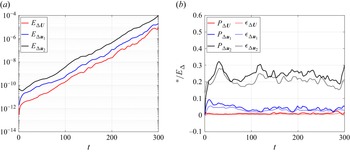


 Open access

