


1. Introduction
Nucleate boiling heat transfer at high pressure is typically used in power generation and nuclear reactors because of its high heat transfer efficiency. For the purpose of designing an effective, efficient and safe system, the boiling heat transfer coefficient and departure from nucleate boiling (DNB), i.e. the maximum heat flux that can be removed by nucleate boiling, can be predicted using empirical or semi-empirical correlations, such as those reviewed by Li et al. (Reference Li, Huang, Qiu, Wang, Yang, Wang and Zhu2025). However, little is known about the mechanisms that determine the effectiveness and trigger the failure of nucleate boiling in high pressure subcooled flow boiling, and large uncertainty margins must be included when designing and operating such systems.
In recent years, the understanding of boiling phenomena has significantly improved thanks to advances in high-resolution measurement techniques developed to capture local parameters such as temperature, heat flux and void fraction on the boiling surface, as well as velocity and temperature distribution in the bulk of the flow. For example, high-speed video and infrared diagnostics have proven particularly valuable, enabling direct observation of bubble dynamics, including heat flux partitioning (mostly at low pressures with water) and nucleation phenomena, e.g. as reported by Richenderfer et al. (Reference Richenderfer, Kossolapov, Seong, Saccone, Demarly, Kommajosyula, Baglietto, Buongiorno and Bucci2018) and Kossolapov et al. (Reference Kossolapov, Chavagnat, Nop, Dorville, Phillips, Buongiorno and Bucci2020). These experimental results can be directly compared with numerical simulations that specifically resolve the liquid–vapour interface, as demonstrated by Kaiser, Sato & Gabriel (Reference Kaiser, Sato and Gabriel2024).
In parallel with measurement techniques, computational fluid dynamics (CFD) simulation methods have also significantly advanced. From the viewpoint of the governing equations, CFD simulation methods for boiling flow can be categorised into two groups: single-fluid and two-fluid/Eulerian approaches.
In the single-fluid approach, just one set of Navier–Stokes equations is solved for the continuum phase, together with the energy conservation equation and an equation to track or resolve the liquid–vapour interface (Hayashi & Tomiyama Reference Hayashi and Tomiyama2018). Since the liquid–vapour interface needs to be resolved and tracked, this approach is sometimes referred to as an interface tracking method (ITM). In boiling flow simulations, it is essential to resolve the liquid–vapour interface shape, because vapourisation and condensation rates are strongly influenced by the temperature distributions near the liquid–vapour interface (Sato, Smith & Niceno Reference Sato, Smith and Niceno2018). Thus, while the single-fluid approach is considered to be the most appropriate for simulations with phase-change phenomena (Yadigaroglu Reference Yadigaroglu2005), very fine computational meshes are required to specifically resolve the interface itself, making simulations computationally very expensive. There are several types of approach within the framework of the single-fluid methodology, e.g. the arbitrary Lagrangian–Eulerian (ALE) approach (Lee & Nydahl Reference Lee and Nydahl1989; Welch Reference Welch1998; Fuchs, Kern & Stephan Reference Fuchs, Kern and Stephan2006), the level-set method (Son, Dhir & Ramanujapu Reference Son, Dhir and Ramanujapu1999; Huber et al. Reference Huber, Tanguy, Sagan and Colin2017; Iskhakova et al. Reference Iskhakova, Kondo, Tanimoto, Dinh and Bolotnov2025), the volume of fluid (VOF) method (Welch & Wilson Reference Welch and Wilson2000; Kunkelmann & Stephan Reference Kunkelmann and Stephan2009; Bureš & Sato Reference Bureš and Sato2021; Saini et al. Reference Saini, Chen, Zaleski and Fuster2024; Long et al. Reference Long, Pan, Cipriano, Bucci and Zaleski2025), the colour function method (Sato & Niceno Reference Sato and Niceno2013; Giustini et al. Reference Giustini, Walker, Sato and Niceno2017), the front tracking method (Esmaeeli & Tryggvason Reference Esmaeeli and Tryggvason2004), the edge-based interface tracking method (Long, Pan & Zaleski Reference Long, Pan and Zaleski2024) and the phase field method (Jamet et al. Reference Jamet, Lebaigue, Coutris and Delhaye2001; Takada & Tomiyama Reference Takada and Tomiyama2007; Badillo Reference Badillo2012). The differences between these approaches lie in the methods used to represent the gas–liquid interface. However, all of them have been applied more or less successfully to the simulation of nucleate boiling and film boiling, as reviewed by Kharangate & Mudawar (Reference Kharangate and Mudawar2017).
ITM has been applied to simulate flow boiling on a heated wall. For instance, Dhir’s group conducted three-dimensional numerical simulations of a single bubble sliding and departing from a heated wall (Dhir, Abarajith & Li Reference Dhir, Abarajith and Li2007; Li & Dhir Reference Li and Dhir2007). The numerical results were compared with the experiments by Maity (Reference Maity2000). Later, the same experiment was simulated by Lal, Sato & Niceno (Reference Lal, Sato and Niceno2015) using an alternative numerical scheme. These simulations partially reproduced bubble growth, sliding and lift-off behaviours consistent with experimental observations, despite the assumption of a constant and uniform wall superheat. Chen et al. (Reference Chen, Ling, Ding, Wang, Jin and Tao2022) simulated subcooled flow boiling of water at 10 ${\rm bar}$
in a horizontal channel of 20
${\rm bar}$
in a horizontal channel of 20 $\times$
2
$\times$
2 $\times$
2 mm
$\times$
2 mm $^3$
. The predicted wall superheat agrees with the Gungor & Winterton (Reference Gungor and Winterton1986) boiling correlation, whereas other quantities, such as void fraction or bubble distribution, were not compared with measurements, and so the validity of these simulations remains unclear. Kaiser et al. (Reference Kaiser, Sato and Gabriel2024) performed both the experiment and CFD simulation of subcooled flow boiling at 2–3
$^3$
. The predicted wall superheat agrees with the Gungor & Winterton (Reference Gungor and Winterton1986) boiling correlation, whereas other quantities, such as void fraction or bubble distribution, were not compared with measurements, and so the validity of these simulations remains unclear. Kaiser et al. (Reference Kaiser, Sato and Gabriel2024) performed both the experiment and CFD simulation of subcooled flow boiling at 2–3 ${\rm bar}$
. Detailed comparisons were made, including wall superheat, velocity profile, bubble diameter distribution and bubble lift-off dynamics. Direct comparison between measurement and simulation revealed the limitations of the CFD simulation: e.g. over-prediction of bubble merging and under-prediction of the condensation process in the bulk flow, these discrepancies primarily due to insufficient grid resolution.
${\rm bar}$
. Detailed comparisons were made, including wall superheat, velocity profile, bubble diameter distribution and bubble lift-off dynamics. Direct comparison between measurement and simulation revealed the limitations of the CFD simulation: e.g. over-prediction of bubble merging and under-prediction of the condensation process in the bulk flow, these discrepancies primarily due to insufficient grid resolution.
ITM, coupled with a phase change model, has also been implemented in unstructured mesh CFD codes, enabling the simulation of boiling flow in complex geometries. Iskhakova et al. (Reference Iskhakova, Kondo, Tanimoto, Dinh and Bolotnov2023, Reference Iskhakova, Kondo, Tanimoto, Dinh and Bolotnov2025) presented simulations of boiling flow of a refrigerant in a vertical rectangular channel with fins using a finite-element CFD code. The use of an unstructured mesh CFD code for boiling simulations was also proposed by Giustini & Issa (Reference Giustini and Issa2021) and El Mellas et al. (Reference El Mellas, Samkhaniani, Falsetti, Stroh, Icardi and Magnini2024).
In two-fluid/Eulerian approaches, the liquid–vapour interface is not directly described, and interfacial forces, heat and mass transfer are computed using closure models. Studies applying the Eulerian approach to subcooled flow boiling have been comprehensively reviewed by Krepper & Ding (Reference Krepper and Ding2023). These models introduce various empirical parameters, such as drag and lift coefficients for interfacial forces, interfacial heat transfer coefficient, nucleation site density, bubble departure diameter and departure frequency for wall boiling. To tune or optimise these parameters so that the computed results match experimental measurements, detailed distributions of temperature and velocity for each phase (liquid and vapour), void fraction and bubble number density are required. An example of a comparative study on modelling was published by Bois et al. (Reference Bois2024), which used the DEBORA database (Garnier, Manon & Cubizolles Reference Garnier, Manon and Cubizolles2001) for validation purposes. Although several experimental measurements can be used for this purpose, as reviewed by Taş (Reference Taş2024), obtaining these distributions remains costly and, in some cases, nearly impossible, particularly the three-dimensional distributions of temperature and velocity in both the liquid and vapour phases. In such cases, simulation data obtained from ITMs could provide invaluable insights and possibly quantitative predictions.
In this paper, we present an ITM simulation of subcooled flow boiling of water at 10.5 ${\rm bar}$
, at an average surface heat flux of 1000 kW m–
${\rm bar}$
, at an average surface heat flux of 1000 kW m– $^2$
, a mass flux of 1000 kg m–
$^2$
, a mass flux of 1000 kg m– $^2$
s–1 and a subcooling degree of 10 K. Due to the high computational cost of the ITM implemented in the open-source, in-house CFD code PSI-BOIL (https://github.com/Niceno/PSI-BOIL), only one simulation case is presented. We emphasise that even a single simulation case required nearly one year of wall-clock time on 128 parallel CPU cores, equivalent to approximately 1.1 million core-hours. The objectives are: (i) to shed light on heat transfer mechanisms in subcooled flow boiling at moderate pressure; and (ii) to validate the simulation method, while providing insights into quantities and mechanisms that are difficult to access experimentally – such as the three-dimensional distributions of velocity, temperature and void fraction, as well as the heat flux partitioning. The simulation also provides detailed spatial data on interfacial mass transfer and bubble number density, offering valuable insights for the development of Eulerian boiling models. We note that a microlayer model (Sato & Niceno Reference Sato and Niceno2015) is not employed in this simulation, since a microlayer was not observed in the experiment, as expected in moderate-pressure conditions.
$^2$
s–1 and a subcooling degree of 10 K. Due to the high computational cost of the ITM implemented in the open-source, in-house CFD code PSI-BOIL (https://github.com/Niceno/PSI-BOIL), only one simulation case is presented. We emphasise that even a single simulation case required nearly one year of wall-clock time on 128 parallel CPU cores, equivalent to approximately 1.1 million core-hours. The objectives are: (i) to shed light on heat transfer mechanisms in subcooled flow boiling at moderate pressure; and (ii) to validate the simulation method, while providing insights into quantities and mechanisms that are difficult to access experimentally – such as the three-dimensional distributions of velocity, temperature and void fraction, as well as the heat flux partitioning. The simulation also provides detailed spatial data on interfacial mass transfer and bubble number density, offering valuable insights for the development of Eulerian boiling models. We note that a microlayer model (Sato & Niceno Reference Sato and Niceno2015) is not employed in this simulation, since a microlayer was not observed in the experiment, as expected in moderate-pressure conditions.
The remainder of the paper is structured as follows: § 2 describes the numerical approach; § 3 presents the grid dependence study performed; § 4 provides the validation and analysis; and § 5 summarises the conclusions.
2. Numerical method
The numerical method is based on a Cartesian grid system in a staggered variable arrangement (Harlow & Welch Reference Harlow and Welch1965). A projection method (Chorin Reference Chorin1968) is used for the coupling of velocity and pressure fields, and a single set of Navier–Stokes equations is solved with an interface tracking method. The Navier–Stokes solver for the two-phase flow is coupled with an energy balance equation solver and a sharp-interface phase-change model (Sato & Niceno Reference Sato and Niceno2013). The vapour and liquid phases are treated as incompressible fluids, and the solid phase is handled with an immersed boundary method (Mittal & Iaccarino Reference Mittal and Iaccarino2005). The method is essentially the same as that developed for previous simulations of pool boiling (Sato & Niceno Reference Sato and Niceno2017, Reference Sato and Niceno2018) and flow boiling (Kaiser et al. Reference Kaiser, Sato and Gabriel2024) conditions, with the primary difference being the updated nucleation site model employed here, which will be presented in § 2.3.
2.1. Navier–Stokes solver
The governing equations are expressed as follows (Sato & Niceno Reference Sato and Niceno2013):
 \begin{align} \boldsymbol{\nabla }\boldsymbol{\cdot }\boldsymbol{u}&=\left ( \frac {1}{{{\rho }_{v}}}-\frac {1}{{{\rho }_{l}}} \right )\dot {m}, \end{align}
 \begin{align} \rho \frac {\partial \boldsymbol{u}}{\partial t}+\rho \left \{ \boldsymbol{\nabla }\boldsymbol{\cdot }\left ( \boldsymbol{u}\otimes \boldsymbol{u} \right )-\boldsymbol{u}\left ( \boldsymbol{\nabla }\boldsymbol{\cdot }\boldsymbol{u} \right ) \right \}&=-\boldsymbol{\nabla }p+\boldsymbol{\nabla }\boldsymbol{\cdot }\left \{ \left ( \mu +{{\mu }_{t}} \right )\left ( \boldsymbol{\nabla }\boldsymbol{u}+{{\left ( \boldsymbol{\nabla }\boldsymbol{u} \right )}^{T}} \right ) \right \}+\boldsymbol{F}, \end{align}
 \begin{align} \frac {\partial \phi }{\partial t}+\boldsymbol{\nabla }\boldsymbol{\cdot }\left ( \phi \boldsymbol{u} \right )&=-\frac {1}{{{\rho }_{l}}}\dot {m}, \end{align}
 \begin{align} {{C}_{p}}\left ( \frac {\partial T}{\partial t}+\boldsymbol{u}\boldsymbol{\cdot }\boldsymbol{\nabla }T \right )&=\boldsymbol{\nabla }\boldsymbol{\cdot }\left ( \left ( \lambda +{{\lambda }_{t}} \right )\boldsymbol{\nabla }T \right )+Q .\end{align}
Equations (2.1)–(2.2) represent the mass and momentum conservation equations, respectively. In these equations, $\boldsymbol{u}$
(m s–1) is the velocity vector,
$\boldsymbol{u}$
(m s–1) is the velocity vector, $\rho$
(
$\rho$
( ${\rm kg\,m}^{-3}$
) the density, and the subscripts
${\rm kg\,m}^{-3}$
) the density, and the subscripts $l$
and
$l$
and $v$
denote the liquid and vapour phases, respectively. Additionally,
$v$
denote the liquid and vapour phases, respectively. Additionally, $\dot {m}\,(\rm kg\,m^{-3}\,s^{-1})$
is the phase change rate, which takes a positive value for vapourisation and a negative value for condensation; t (s) denotes time, p (Pa) is pressure;
$\dot {m}\,(\rm kg\,m^{-3}\,s^{-1})$
is the phase change rate, which takes a positive value for vapourisation and a negative value for condensation; t (s) denotes time, p (Pa) is pressure; $\mu$
(
$\mu$
( ${\rm Pa\,s}$
) is the dynamic molecular viscosity;
${\rm Pa\,s}$
) is the dynamic molecular viscosity; $\mu _t ({\rm Pa\,s})$
is the turbulent eddy viscosity; and
$\mu _t ({\rm Pa\,s})$
is the turbulent eddy viscosity; and $\boldsymbol{F}$
(
$\boldsymbol{F}$
( ${\rm N\,m}^{-3}$
) is the body-force vector. Equation (2.3) is the governing equation for the liquid volume fraction
${\rm N\,m}^{-3}$
) is the body-force vector. Equation (2.3) is the governing equation for the liquid volume fraction $\phi$
, which quantifies the volume fraction of liquid within a given control volume. The average density and viscosity in a control volume (i.e. a computational cell in this formulation) are respectively defined as
$\phi$
, which quantifies the volume fraction of liquid within a given control volume. The average density and viscosity in a control volume (i.e. a computational cell in this formulation) are respectively defined as
 \begin{equation} \rho ={{\phi }_{{}}}{{\rho }_{l}}+\left ( 1-\phi \right ){{\rho }_{v}} \quad \text{and} \quad \mu ={{\phi }_{{}}}{{\mu }_{l}}+\left ( 1-\phi \right ){{\mu }_{v}}. \end{equation}
The advection term in (2.3) is discretised according to the rational CIP-CSL2 scheme (Xiao, Yabe & Ito Reference Xiao, Yabe and Ito1996; Nakamura et al. Reference Nakamura, Tanaka, Yabe and Takizawa2001). To prevent smearing of the liquid volume fraction $\phi$
, an interface sharpening algorithm (Sato & Niceno Reference Sato and Niceno2012) is employed. Equation (2.4) is the energy balance equation, in which
$\phi$
, an interface sharpening algorithm (Sato & Niceno Reference Sato and Niceno2012) is employed. Equation (2.4) is the energy balance equation, in which $C_p=\rho c_p$
(J
$C_p=\rho c_p$
(J ${\rm m^{-3}\,K^{-1}}$
) is the volumetric specific heat capacity at constant pressure,
${\rm m^{-3}\,K^{-1}}$
) is the volumetric specific heat capacity at constant pressure, $T$
(K) the temperature,
$T$
(K) the temperature, $\lambda$
(W m–1K–1) the thermal conductivity,
$\lambda$
(W m–1K–1) the thermal conductivity, $\lambda _t$
(W m–1K–1) the turbulent thermal conductivity and
$\lambda _t$
(W m–1K–1) the turbulent thermal conductivity and $Q$
(
$Q$
( ${\rm W\,m^{-3}}$
) the volumetric heat source. The specific heat capacity and the thermal conductivity for the liquid and vapour phases are defined as
${\rm W\,m^{-3}}$
) the volumetric heat source. The specific heat capacity and the thermal conductivity for the liquid and vapour phases are defined as
 \begin{equation} C_p = \begin{cases} C_{pl} & \text{for a cell with } \phi \geqslant 0.5,\\ C_{pv} & \text{for a cell with } \phi \lt 0.5, \end{cases} \quad \lambda = \begin{cases} \lambda _l & \text{for a cell with } \phi \geqslant 0.5,\\ \lambda _v & \text{for a cell with } \phi \lt 0.5. \end{cases} \end{equation}
The turbulent thermal conductivity is calculated according to $Pr_t = (\mu _t/\rho )/(\lambda _t/C_p)$
, where
$Pr_t = (\mu _t/\rho )/(\lambda _t/C_p)$
, where $Pr_t(= 0.9)$
is the turbulent Prandtl number. Detailed derivations of (2.1)–(2.4) are given in Appendices A and B of Sato & Niceno (Reference Sato and Niceno2013).
$Pr_t(= 0.9)$
is the turbulent Prandtl number. Detailed derivations of (2.1)–(2.4) are given in Appendices A and B of Sato & Niceno (Reference Sato and Niceno2013).
Turbulence is modelled here using large eddy simulation (LES), the Smagorinsky subgrid-scale model (Smagorinsky Reference Smagorinsky1963) being adopted to estimate the turbulent eddy viscosity $\mu _t$
:
$\mu _t$
:
 \begin{equation} {{\mu }_{t}}=\rho {{\left ( {{C}_{s}}d\bar {\Delta } \right )}^{2}}\sqrt {2\left ( {{{\bar {S}}}_{\textit{ij}}}{{{\bar {S}}}_{\textit{ij}}} \right )}, \end{equation}
where $C_s = 0.17$
is the Smagorinsky constant, the value being derived by Lilly (Reference Lilly1967);,
$C_s = 0.17$
is the Smagorinsky constant, the value being derived by Lilly (Reference Lilly1967);, ${\bar {S}}_{\textit{ij}}$
the strain-rate tensor defined as
${\bar {S}}_{\textit{ij}}$
the strain-rate tensor defined as ${{\bar {S}}_{\textit{ij}}}=({1}/{2}) ({\partial {{u}_{i}}}/{\partial {{x}_{\!j}}})+({\partial {{u}_{\!j}}}/{\partial {{x}_{i}}} )$
;
${{\bar {S}}_{\textit{ij}}}=({1}/{2}) ({\partial {{u}_{i}}}/{\partial {{x}_{\!j}}})+({\partial {{u}_{\!j}}}/{\partial {{x}_{i}}} )$
; $\bar {\Delta }$
the filter width defined as
$\bar {\Delta }$
the filter width defined as $\bar {\Delta }={{ ( \Delta x\Delta y\Delta z )}^{{}^{1}/{}_{3}}}$
,
$\bar {\Delta }={{ ( \Delta x\Delta y\Delta z )}^{{}^{1}/{}_{3}}}$
, $\Delta x$
,
$\Delta x$
, $\Delta y$
and
$\Delta y$
and $\Delta z$
being the cell size in the
$\Delta z$
being the cell size in the $x$
-,
$x$
-, $y$
- and
$y$
- and $z$
-directions, respectively. Finally,
$z$
-directions, respectively. Finally, $d$
is the near wall damping function proposed by Inagaki, Kondoh & Nagano (Reference Inagaki, Kondoh and Nagano2002):
$d$
is the near wall damping function proposed by Inagaki, Kondoh & Nagano (Reference Inagaki, Kondoh and Nagano2002):
 \begin{equation} d = \sqrt {1 - e^{\left ( -y^+ / 25 \right )^3}}. \end{equation}
Here, ${y}^{+}$
is the non-dimensional distance from the wall surface to the cell centre. We do not model turbulence–interface coupling; reliable closures for turbulence at phase-changing interfaces are not yet available (Kharangate & Mudawar Reference Kharangate and Mudawar2017).
${y}^{+}$
is the non-dimensional distance from the wall surface to the cell centre. We do not model turbulence–interface coupling; reliable closures for turbulence at phase-changing interfaces are not yet available (Kharangate & Mudawar Reference Kharangate and Mudawar2017).
On the right-hand side of (2.2), the body-force vector $\boldsymbol{F}$
includes both gravity and surface tension forces. The surface tension coefficient
$\boldsymbol{F}$
includes both gravity and surface tension forces. The surface tension coefficient $\sigma$
is set to a constant value at the saturation temperature, meaning that the Marangoni effect (Burdon Reference Burdon1949) is neglected in the simulations. Brackbill’s continuum surface force (CSF) model (Brackbill, Kothe & Zemach Reference Brackbill, Kothe and Zemach1992) is employed to represent the effects of surface tension. To mitigate strong parasitic currents, we employ the density-scaled form of the CSF model (Brackbill et al. Reference Brackbill, Kothe and Zemach1992).
$\sigma$
is set to a constant value at the saturation temperature, meaning that the Marangoni effect (Burdon Reference Burdon1949) is neglected in the simulations. Brackbill’s continuum surface force (CSF) model (Brackbill, Kothe & Zemach Reference Brackbill, Kothe and Zemach1992) is employed to represent the effects of surface tension. To mitigate strong parasitic currents, we employ the density-scaled form of the CSF model (Brackbill et al. Reference Brackbill, Kothe and Zemach1992).
The same governing energy equation (2.4) is solved for both the fluid and solid domains, where the convection term automatically vanishes in the latter due to the zero velocity. The thermal diffusion coefficient is assigned the value of the solid material and the heater power is applied as a volumetric heat source, $Q$
.
$Q$
.
2.2. Phase change model
The phase-change rate at the liquid–vapour interface is computed directly from the heat fluxes on the two sides. The temperature at the liquid–vapour interface is assumed to be the saturation temperature at the prevailing pressure, though away from the interface, the conditions of superheated liquid and subcooled vapour are properly taken into account. The phase change rate $\dot {m}$
at the liquid–vapour interface is modelled as
$\dot {m}$
at the liquid–vapour interface is modelled as
 \begin{equation} \dot {m}=\frac {{{q}_{l}}+{{q}_{v}}}{\mathscr{h}_{lv}}\frac {{{S}_{\textit{int}}}}{V}, \end{equation}
where $q_l$
and
$q_l$
and $q_v$
are the heat fluxes (W m–2) derived from the liquid and the vapour sides of the interface, respectively;
$q_v$
are the heat fluxes (W m–2) derived from the liquid and the vapour sides of the interface, respectively; $\mathscr{h}_{lv}$
(J kg–1) is the latent heat of vapourisation;
$\mathscr{h}_{lv}$
(J kg–1) is the latent heat of vapourisation; $S_{\textit{int}}$
(
$S_{\textit{int}}$
( ${m}^{2}$
) the area of the liquid–vapour interface in the computational cell under consideration; and
${m}^{2}$
) the area of the liquid–vapour interface in the computational cell under consideration; and $V$
(
$V$
( ${m}^{3}$
) is the cell volume. The area
${m}^{3}$
) is the cell volume. The area $S_{\textit{int}}$
is calculated by means of the marching cube algorithm (Lorensen & Cline Reference Lorensen and Cline1987), which has been proven successful for this type of flow (Sato & Niceno Reference Sato and Niceno2013). The heat fluxes at the interface are defined as
$S_{\textit{int}}$
is calculated by means of the marching cube algorithm (Lorensen & Cline Reference Lorensen and Cline1987), which has been proven successful for this type of flow (Sato & Niceno Reference Sato and Niceno2013). The heat fluxes at the interface are defined as ${{q}_{l}}= ( {{\lambda }_{l}}+{{\lambda }_{t}} ) ( \boldsymbol{\nabla }{{T}_{l}} )\boldsymbol{\cdot }\boldsymbol{n}$
and
${{q}_{l}}= ( {{\lambda }_{l}}+{{\lambda }_{t}} ) ( \boldsymbol{\nabla }{{T}_{l}} )\boldsymbol{\cdot }\boldsymbol{n}$
and ${{q}_{v}}=- ( {{\lambda }_{v}}+{{\lambda }_{t}} ) ( \boldsymbol{\nabla }{{T}_{v}} )\boldsymbol{\cdot }\boldsymbol{n}$
, where
${{q}_{v}}=- ( {{\lambda }_{v}}+{{\lambda }_{t}} ) ( \boldsymbol{\nabla }{{T}_{v}} )\boldsymbol{\cdot }\boldsymbol{n}$
, where ${T}_{l}$
and
${T}_{l}$
and ${T}_{v}$
are the temperatures in the liquid and vapour phases, respectively. Here,
${T}_{v}$
are the temperatures in the liquid and vapour phases, respectively. Here, $\boldsymbol{n}$
is the unit normal vector to the interface, pointing from the vapour to the liquid phase. Note that the temperature defined in cells filled with liquid phase and the temperature at the liquid–vapour interface are both used for the computation of
$\boldsymbol{n}$
is the unit normal vector to the interface, pointing from the vapour to the liquid phase. Note that the temperature defined in cells filled with liquid phase and the temperature at the liquid–vapour interface are both used for the computation of $\boldsymbol{\nabla }{{T}_{l}}$
, and the same is true for the vapour phase. More details of the sharp-interface phase-change model can be found from Sato & Niceno (Reference Sato and Niceno2013).
$\boldsymbol{\nabla }{{T}_{l}}$
, and the same is true for the vapour phase. More details of the sharp-interface phase-change model can be found from Sato & Niceno (Reference Sato and Niceno2013).
2.3. Nucleation-site model
In the present numerical method, a description of the liquid–vapour interface is essential for phase change. Without it, $S_{\textit{int}}$
in (2.9) becomes zero and no phase change occurs. Therefore, a nucleation-site model has been developed to introduce such an interface and initiate nucleate boiling.
$S_{\textit{int}}$
in (2.9) becomes zero and no phase change occurs. Therefore, a nucleation-site model has been developed to introduce such an interface and initiate nucleate boiling.
(a) Flowchart illustrating the procedure for defining nucleation-site locations and associated activation temperatures $T_{act}$
and (b) the experimentally derived relationship between the number of active nucleation sites and wall temperature.
$T_{act}$
and (b) the experimentally derived relationship between the number of active nucleation sites and wall temperature.

2.3.1. Defining nucleation-site locations and assigning activation temperatures
As a preliminary to the CFD simulation, we prescribe the locations of the nucleation sites on the heat transfer surface, together with a nucleation activation temperature $T_{act}$
. The methodology for defining the nucleation site locations, and the corresponding values for
$T_{act}$
. The methodology for defining the nucleation site locations, and the corresponding values for ${T}_{act}$
, is illustrated in flowchart form in figure 1(a). Initially, the counter for the nucleation site is set to 1. The activation temperature for Site #1 (
${T}_{act}$
, is illustrated in flowchart form in figure 1(a). Initially, the counter for the nucleation site is set to 1. The activation temperature for Site #1 ( ${T}_{act,\#1}$
) is obtained from the relationship between the number of active nucleation sites and the wall temperature, as read off using the trend line shown in figure 1(b), which is obtained from active nucleation site density (NSD) measured in an experiment. The abscissa represents the number of nucleation sites 1, 2, 3,
${T}_{act,\#1}$
) is obtained from the relationship between the number of active nucleation sites and the wall temperature, as read off using the trend line shown in figure 1(b), which is obtained from active nucleation site density (NSD) measured in an experiment. The abscissa represents the number of nucleation sites 1, 2, 3, $\ldots, m$
, spaced evenly, the final number
$\ldots, m$
, spaced evenly, the final number $m$
being determined by the maximum activation temperature,
$m$
being determined by the maximum activation temperature, $T_{max}$
, on the upper heater surface. Hence, the total number of nucleation sites ultimately depends on the magnitude of the applied heat flux and, as will be described later, this process is self-controlled, as implemented here. The nucleation site selection procedure begins with the first site, Site #1, its location being chosen using a (unbiased) random number generator, so could be positioned anywhere on the heat transfer surface. The associated activation temperature for this site is then read off from figure 1(b).
$T_{max}$
, on the upper heater surface. Hence, the total number of nucleation sites ultimately depends on the magnitude of the applied heat flux and, as will be described later, this process is self-controlled, as implemented here. The nucleation site selection procedure begins with the first site, Site #1, its location being chosen using a (unbiased) random number generator, so could be positioned anywhere on the heat transfer surface. The associated activation temperature for this site is then read off from figure 1(b).
The second nucleation, Site #2, then needs to be defined, again via a random number generator. The counter for the number of nucleation sites is increased (i.e. $i = i+1$
) and the associated activation temperature for this site is obtained from figure 1(b), as before. Note that
$i = i+1$
) and the associated activation temperature for this site is obtained from figure 1(b), as before. Note that ${T}_{act,\#2}$
is greater than
${T}_{act,\#2}$
is greater than ${T}_{act,\#1}$
. This process is continued until the activation temperature at Site
${T}_{act,\#1}$
. This process is continued until the activation temperature at Site $\#m$
(figure 1
b) exceeds
$\#m$
(figure 1
b) exceeds ${T}_{max}$
, which is chosen higher than the maximum wall temperature anticipated in the simulation. It is to be recalled that the nucleation process is controlled by the local heat-transfer surface temperature, which is itself determined from the applied heat flux.
${T}_{max}$
, which is chosen higher than the maximum wall temperature anticipated in the simulation. It is to be recalled that the nucleation process is controlled by the local heat-transfer surface temperature, which is itself determined from the applied heat flux.
The active NSD is obtained from the measurements presented in figures 5–11 of Kossolapov (Reference Kossolapov2021), and is subsequently used in (3.2) and illustrated in figure 5. The maximum activation temperature ${T}_{max}$
was set to
${T}_{max}$
was set to $T_{\textit{sat}} + 21.5\,\rm K$
, which corresponds to
$T_{\textit{sat}} + 21.5\,\rm K$
, which corresponds to $NSD = {10}^{9}\,({\rm m}^{-2})$
. Here, 21.5 K is sufficiently higher than the 7 K wall superheat observed in the measured boiling curve. This concludes the pre-processing stage.
$NSD = {10}^{9}\,({\rm m}^{-2})$
. Here, 21.5 K is sufficiently higher than the 7 K wall superheat observed in the measured boiling curve. This concludes the pre-processing stage.
2.3.2. Activation criteria and seed-bubble initialisation
In the nucleation-site model, a small vapour seed bubble is introduced at a nucleation site when:
-
(i) the local temperature at the nucleation site reaches $T_{act}$
; and
$T_{act}$
; and -
(ii) the fluid above the site is in the liquid phase.

The seed bubble is initially assumed to be spherical, with a diameter set to 2.4 times the grid cell width of the underlying grid $ ( =2.4\boldsymbol{\cdot }\max ( \Delta x,\Delta y,\Delta z ) )$
. Although the initial bubble shape is physically influenced by factors such as wettability, fluid properties, system pressure, applied heat flux and flow conditions, a spherical shape was chosen based on the observations of nucleate boiling of water at moderate pressure reported by Sakashita (Reference Sakashita2011) and Kossolapov et al. (Reference Kossolapov, Hughes, Phillips and Bucci2024). The dependence of the seed bubble diameter on the cell size inherently makes the model sensitive to the grid spacing chosen. Consequently, a grid refinement study is necessary to evaluate the impact of this assumption on the accuracy of the results.
$ ( =2.4\boldsymbol{\cdot }\max ( \Delta x,\Delta y,\Delta z ) )$
. Although the initial bubble shape is physically influenced by factors such as wettability, fluid properties, system pressure, applied heat flux and flow conditions, a spherical shape was chosen based on the observations of nucleate boiling of water at moderate pressure reported by Sakashita (Reference Sakashita2011) and Kossolapov et al. (Reference Kossolapov, Hughes, Phillips and Bucci2024). The dependence of the seed bubble diameter on the cell size inherently makes the model sensitive to the grid spacing chosen. Consequently, a grid refinement study is necessary to evaluate the impact of this assumption on the accuracy of the results.
Upon nucleation, the seed bubble is initialised as follows.
-
(i) The liquid volume fraction in the corresponding region is changed from liquid to vapour phase.
-
(ii) The velocity field in the seed bubble remains unchanged.
-
(iii) The temperature in the seed bubble is set to
$T_{\textit{sat}}$
, assuming no superheated vapour inside an initial bubble. -
(iv) The latent heat required for the seed bubble formation (
$\rho _v V_b L$
) is subtracted from the solid cells beneath the bubble, where
$V_b$
is the bubble volume.


We acknowledge that these procedures have room for improvement. Mass and energy conservations are violated, although a small seed bubble diameter (2.4 times the grid cell width) was chosen to minimise their impact. Additionally, the velocity field in the seed bubble could be approximated more physically.
In item (iv), performing latent heat subtraction in a single time step can lower the solid temperature below $T_{\textit{sat}}$
, which is considered unphysical and may lead to immediate condensation. To prevent this, latent heat subtraction is gradually applied over multiple time steps, introducing a heat sink in the energy equation, ensuring the solid temperature always remains above
$T_{\textit{sat}}$
, which is considered unphysical and may lead to immediate condensation. To prevent this, latent heat subtraction is gradually applied over multiple time steps, introducing a heat sink in the energy equation, ensuring the solid temperature always remains above $T_{\textit{sat}}$
. Once the cumulative heat sink over the time integration reaches the latent heat (
$T_{\textit{sat}}$
. Once the cumulative heat sink over the time integration reaches the latent heat ( $\rho _v V_b L$
), then the seed bubble is planted as illustrated in the schematic in figure 2. The number of time steps required for the latent heat subtraction depends on the evolution of the wall temperature
$\rho _v V_b L$
), then the seed bubble is planted as illustrated in the schematic in figure 2. The number of time steps required for the latent heat subtraction depends on the evolution of the wall temperature $T_w$
, which is influenced by the flow field, heater power, time increment
$T_w$
, which is influenced by the flow field, heater power, time increment $\Delta t$
and other simulation conditions. Thus, this number is not prescribed, but is dynamically determined during the simulation. In the large domain simulation (§ 4), the number of time steps required was 225
$\Delta t$
and other simulation conditions. Thus, this number is not prescribed, but is dynamically determined during the simulation. In the large domain simulation (§ 4), the number of time steps required was 225 $\pm$
40 (standard deviation).
$\pm$
40 (standard deviation).
Procedure of bubble nucleation.

2.3.3. Surface-condition effects
We conclude this section by detailing how our nucleation-site model accounts for surface conditions (roughness, oxidation) and for non-condensable gas dissolved in the liquid. The surface condition is known to significantly influence boiling heat transfer (Rohsenow Reference Rohsenow1971). Empirical correlations, such as those proposed by Jones, McHale & Garimella (Reference Jones, McHale and Garimella2009), indicate that roughened surfaces increase the number of nucleation sites and the size of surface cavities, thereby enhancing boiling heat transfer. In the present NSD model, this effect is accounted for indirectly by using the experimentally measured active NSD as input. By construction, the measured NSD already embodies the influence of surface conditions and dissolved non-condensable gas. In cases where experimental data are not available, correlations for the nucleation site density – for example, those proposed by Kocamustafaogullari & Ishii (Reference Kocamustafaogullari and Ishii1983) or Hibiki & Ishii (Reference Hibiki and Ishii2003) – may be used.
2.4. Assumptions
The assumptions used in the numerical method are summarised here for clarity.
-
(i) The working fluid is assumed to be incompressible.
-
(ii) The temperature at the liquid–vapour interface is assumed to remain constant and equal to the saturation temperature,
$T_{\textit{sat}}$
, at the prevailing pressure. The pressure inside small bubbles theoretically increases due to the Laplace pressure, which leads to a slightly higher saturation temperature. However, the smallest bubbles computed in this study are seed bubbles with a diameter of
$47\,\unicode{x03BC}{\rm m}$
(
$=2.4\,\times$
grid spacing for the validation case; see § 4), corresponding to a Laplace pressure of approximately
$0.05\,{\rm bar}$
and an increase in saturation temperature of approximately
$0.2\,\rm K$
. Although this temperature rise is not entirely negligible, the saturation temperature was fixed to a constant value to avoid numerical instabilities arising from pressure fluctuations. Consequently, the Marangoni effect is neglected. -
(iii) Only the heat-transfer-controlled bubble growth is considered, as the seed bubble size is already larger than the range corresponding to inertia-controlled growth. The bubble size corresponding to the transition between inertia and heat-transfer-controlled growth is estimated to be approximately
$0.2\,\unicode{x03BC}{\rm m}$
for water at
$10.5\,\rm bar$
, assuming a liquid superheat of
$5\,\rm K$
(Carey Reference Carey2008). -
(iv) Radiation heat-transfer is not taken into account, which may limit the accuracy of the computation in the film-boiling regime, especially for high wall-temperature scenarios, which are, however, beyond the scope of this paper.
-
(v) Finally, in the nucleation-site model, each nucleation site is assumed to have a specific nucleation activation temperature,
$T_{act}$
. When the wall temperature at a given nucleation site reaches
$T_{\textit{sat}}$
, a spherical vapour seed bubble is artificially placed at that location.


3. Verification: grid dependence study
To verify the numerical method, a grid dependence study has been undertaken. The conditions of the simulation were based on the experiment conducted at the Massachusetts Institute of Technology (MIT), (Kossolapov Reference Kossolapov2021), which involved upward vertical flow in a square channel with a cross-section 11.78 $\times$
11.78
$\times$
11.78 ${\rm mm}^{2}$
. A 0.7
${\rm mm}^{2}$
. A 0.7 $\unicode{x03BC}{\rm m}$
thick indium tin oxide (ITO) heater with an effective area of 10
$\unicode{x03BC}{\rm m}$
thick indium tin oxide (ITO) heater with an effective area of 10 $\times$
10
$\times$
10 ${\rm mm}^{2}$
was placed on one side of the channel. The ITO heater was coated on a 1 mm thick sapphire substrate. The time-averaged temperature distribution of the ITO heater was measured using a high-speed infrared (IR) camera, while the liquid or vapour phases on the heater surface were detected with a high-resolution phase detection technique to track vapour and liquid phases on the boiling surface (Kossolapov, Phillips & Bucci Reference Kossolapov, Phillips and Bucci2021). Kossolapov (Reference Kossolapov2021) reported measurements with system pressures ranging from 10 to 40
${\rm mm}^{2}$
was placed on one side of the channel. The ITO heater was coated on a 1 mm thick sapphire substrate. The time-averaged temperature distribution of the ITO heater was measured using a high-speed infrared (IR) camera, while the liquid or vapour phases on the heater surface were detected with a high-resolution phase detection technique to track vapour and liquid phases on the boiling surface (Kossolapov, Phillips & Bucci Reference Kossolapov, Phillips and Bucci2021). Kossolapov (Reference Kossolapov2021) reported measurements with system pressures ranging from 10 to 40 ${\rm bar}$
, mass flux between 500 and 2000 kg m
${\rm bar}$
, mass flux between 500 and 2000 kg m $^{-2}$
s–1, and applied heat fluxes ranging from 1 to 6 MW m
–
$^{-2}$
s–1, and applied heat fluxes ranging from 1 to 6 MW m
– $^2$
.
$^2$
.
3.1. Conditions of simulation
We selected the case at 10.5 ${\rm bar}$
with an applied heat flux of 1000 kW m
–
${\rm bar}$
with an applied heat flux of 1000 kW m
– $^2$
, a mass flux of 1000 kg m
–
$^2$
, a mass flux of 1000 kg m
– $^2$
s–1 and a subcooling degree of 10 K due to the availability of detailed data (Kossolapov Reference Kossolapov2021), which will also be used for the validation in § 4. The physical properties of water and the sapphire substrate, used in the simulations described in §§ 3 and 4, are summarised in table 1.
$^2$
s–1 and a subcooling degree of 10 K due to the availability of detailed data (Kossolapov Reference Kossolapov2021), which will also be used for the validation in § 4. The physical properties of water and the sapphire substrate, used in the simulations described in §§ 3 and 4, are summarised in table 1.
Physical properties of water at 10.5 ${\rm bar}$
and those of the sapphire substrate.
${\rm bar}$
and those of the sapphire substrate.

3.1.1. Computational domain
The computational domain size for the grid dependence study measures 1.25 $\times$
0.63
$\times$
0.63 $\times$
0.39 mm
$\times$
0.39 mm $^3$
in the axial (
$^3$
in the axial ( $x$
-), spanwise (
$x$
-), spanwise ( $y$
-) and wall-normal (
$y$
-) and wall-normal ( $z$
-) directions, respectively, as illustrated in figure 3. The origin of the coordinate system is located on the inlet plane, at the centre of the spanwise direction and on the wall surface. Gravity is applied in the negative
$z$
-) directions, respectively, as illustrated in figure 3. The origin of the coordinate system is located on the inlet plane, at the centre of the spanwise direction and on the wall surface. Gravity is applied in the negative $x$
-direction. This domain is smaller than the experimental test section due to the significant computational resources required for fine-grid simulations. Consequently, the computed results from the grid dependence study cannot be directly compared with experimental measurement. Instead, the results are compared across different grid sizes. Note that a simulation covering the full vertical length of the heated surface in the experiment, i.e. 10 mm, will be conducted in § 4.
$x$
-direction. This domain is smaller than the experimental test section due to the significant computational resources required for fine-grid simulations. Consequently, the computed results from the grid dependence study cannot be directly compared with experimental measurement. Instead, the results are compared across different grid sizes. Note that a simulation covering the full vertical length of the heated surface in the experiment, i.e. 10 mm, will be conducted in § 4.
Computational domain, boundary conditions and distribution of nucleation sites coloured with their activation temperature, $T_{act}$
, for the grid dependence study.
$T_{act}$
, for the grid dependence study.

3.1.2. Boundary conditions
Inlet boundary. A velocity inlet boundary condition is imposed on the surface corresponding to the minimum $x$
-coordinate. Prior to the boiling simulations conducted with the PSI-BOIL code, a preliminary two-dimensional (2-D) steady-state, single-phase liquid flow simulation was performed using ANSYS Fluent 2022 (Ansys 2022). It is important to note that ANSYS Fluent was used exclusively to determine the inlet velocity; all subsequent simulations presented in this study were carried out using the PSI-BOIL code. The computational domain for the 2-D simulation measured 1178.0
$x$
-coordinate. Prior to the boiling simulations conducted with the PSI-BOIL code, a preliminary two-dimensional (2-D) steady-state, single-phase liquid flow simulation was performed using ANSYS Fluent 2022 (Ansys 2022). It is important to note that ANSYS Fluent was used exclusively to determine the inlet velocity; all subsequent simulations presented in this study were carried out using the PSI-BOIL code. The computational domain for the 2-D simulation measured 1178.0 $\times$
5.89
$\times$
5.89 ${\rm mm}^{2}$
in the streamwise and wall-normal directions, respectively, and was discretised using a structured mesh of 2000
${\rm mm}^{2}$
in the streamwise and wall-normal directions, respectively, and was discretised using a structured mesh of 2000 $\times$
200 rectangular cells. The streamwise domain length corresponds to 200
$\times$
200 rectangular cells. The streamwise domain length corresponds to 200 $h$
, where
$h$
, where $h$
is the half-channel height, and was chosen to allow the turbulent flow to become fully developed before the outlet. At the inlet, a uniform velocity profile was prescribed, while a pressure outlet boundary condition was imposed at the outlet, where the pressure was fixed to zero. A no-slip wall boundary condition was applied at the wall and a symmetry condition was used on the opposite side. The SST
$h$
is the half-channel height, and was chosen to allow the turbulent flow to become fully developed before the outlet. At the inlet, a uniform velocity profile was prescribed, while a pressure outlet boundary condition was imposed at the outlet, where the pressure was fixed to zero. A no-slip wall boundary condition was applied at the wall and a symmetry condition was used on the opposite side. The SST $k$
–
$k$
– $\omega$
turbulence model was employed. The minimum mesh spacing near the wall was 5
$\omega$
turbulence model was employed. The minimum mesh spacing near the wall was 5 $\unicode{x03BC}{\rm m}$
; a non-dimensional wall distance of
$\unicode{x03BC}{\rm m}$
; a non-dimensional wall distance of ${y}^{+}$
equals to 0.7. The computed friction Reynolds number at the outlet boundary was
${y}^{+}$
equals to 0.7. The computed friction Reynolds number at the outlet boundary was $Re_{tau} = 1840$
. From the profiles of velocity, turbulent viscosity, turbulent kinetic energy and turbulent dissipation rate at the outlet boundary computed with ANSYS Fluent, the transient inlet velocity field for the boiling simulations with PSI-BOIL was generated using the synthetic eddy method (Jarrin et al. Reference Jarrin, Benhamadouche, Laurence and Prosser2006). The implementation of the synthetic eddy method and its assessment for a single-phase liquid flow are provided in Appendix A.
$Re_{tau} = 1840$
. From the profiles of velocity, turbulent viscosity, turbulent kinetic energy and turbulent dissipation rate at the outlet boundary computed with ANSYS Fluent, the transient inlet velocity field for the boiling simulations with PSI-BOIL was generated using the synthetic eddy method (Jarrin et al. Reference Jarrin, Benhamadouche, Laurence and Prosser2006). The implementation of the synthetic eddy method and its assessment for a single-phase liquid flow are provided in Appendix A.
The inlet temperature was set to a constant value of $(T_{\textit{sat}}-10)\,\rm K$
, with only the liquid phase entering the domain, i.e. no vapour phase was present at the inlet. Here,
$(T_{\textit{sat}}-10)\,\rm K$
, with only the liquid phase entering the domain, i.e. no vapour phase was present at the inlet. Here, $T_{\textit{sat}}$
is the saturation temperature of water at 10.5
$T_{\textit{sat}}$
is the saturation temperature of water at 10.5 ${\rm bar}$
. The Neumann boundary condition is applied for pressure at the inlet.
${\rm bar}$
. The Neumann boundary condition is applied for pressure at the inlet.
Side and symmetry boundaries. A periodic boundary condition was applied to the surfaces at the minimum and maximum $y$
-directions, while a symmetry boundary condition was imposed on the surface at the maximum
$y$
-directions, while a symmetry boundary condition was imposed on the surface at the maximum $z$
-direction, as illustrated in figure 3.
$z$
-direction, as illustrated in figure 3.
Outlet boundary. To ensure the stable release of bubbles without numerical instability from the computational domain, an outlet region was introduced in a manner similar to that described in § 6.1.4 of Sato & Niceno (Reference Sato and Niceno2013). The liquid phase is artificially transformed to vapour without volume change, thereby preventing the liquid–vapour interface from reaching the outlet boundary. Although the opposite treatment (vapour-to-liquid conversion) is also possible, we intentionally use the liquid-to-vapour conversion to avoid liquid-over-vapour stratification under gravity, which could promote Rayleigh–Taylor instability in the outlet region. The liquid volume fraction $\phi$
calculated with the Navier–Stokes solver
$\phi$
calculated with the Navier–Stokes solver $\phi _{\textit{cal}}$
is artificially transformed to
$\phi _{\textit{cal}}$
is artificially transformed to $\phi _{\textit{trans}}$
using the next interpolation:
$\phi _{\textit{trans}}$
using the next interpolation:
 \begin{equation} {{\phi }_{\textit{trans}}}=\left ( 1-c \right ){{\phi }_{\textit{cal}}}, \end{equation}
where the coefficient $c$
is defined as
$c$
is defined as $c={ ( x-{{x}_{1}} )}/{ ( {{x}_{2}}-{{x}_{1}} )}$
,
$c={ ( x-{{x}_{1}} )}/{ ( {{x}_{2}}-{{x}_{1}} )}$
, $x_1$
and
$x_1$
and $x_2$
being the
$x_2$
being the $x$
-coordinates marking the start and end of the outlet region, respectively (see also figure 3). At the outlet boundary, corresponding to the maximum
$x$
-coordinates marking the start and end of the outlet region, respectively (see also figure 3). At the outlet boundary, corresponding to the maximum $x$
-surface, a Neumann condition is applied to the velocity, pressure and the temperature fields.
$x$
-surface, a Neumann condition is applied to the velocity, pressure and the temperature fields.
Boundaries for solid phase. The boundary conditions for the solid domain are as follows: an adiabatic condition is applied to all surfaces except for the wall surface adjacent to the fluid domain. Conjugate heat transfer is solved at the heat transfer surface by solving the energy balance (2.4). A heat source is assigned to the solid cells adjacent to the fluid domain, representing the ITO heater. The thickness of the ITO heater is 0.7 $\unicode{x03BC}{\rm m}$
, consistent with the experimental set-up. However, for simplicity, the physical properties of these cells are assumed to be those of sapphire.
$\unicode{x03BC}{\rm m}$
, consistent with the experimental set-up. However, for simplicity, the physical properties of these cells are assumed to be those of sapphire.
Contact angle. The heat transfer surface is modelled as perfectly hydrophilic; that is, the contact angle in the CSF model (Brackbill et al. Reference Brackbill, Kothe and Zemach1992) is set to zero ( ${{\theta }_{eq}}=0$
) for the following three reasons. First, vapour bubbles observed in experiments conducted under moderate pressure (
${{\theta }_{eq}}=0$
) for the following three reasons. First, vapour bubbles observed in experiments conducted under moderate pressure ( $\geqslant$
10.5
$\geqslant$
10.5 ${\rm bar}$
) exhibit very low apparent contact angles, as shown in figure 4. The bottom view (through the ITO and substrate) of vapour bubbles nucleated and growing on the ITO surface in our subcooled flow boiling experiment (Kossolapov Reference Kossolapov2021), shown in figure 4(a), features a small dry area compared with the bubble diameter, indicating a small apparent contact angle. It should be noted that the static contact angle of a water droplet on the ITO surface measured in our experiment exhibits slightly hydrophilic behaviour, i.e. the angle is slightly below
${\rm bar}$
) exhibit very low apparent contact angles, as shown in figure 4. The bottom view (through the ITO and substrate) of vapour bubbles nucleated and growing on the ITO surface in our subcooled flow boiling experiment (Kossolapov Reference Kossolapov2021), shown in figure 4(a), features a small dry area compared with the bubble diameter, indicating a small apparent contact angle. It should be noted that the static contact angle of a water droplet on the ITO surface measured in our experiment exhibits slightly hydrophilic behaviour, i.e. the angle is slightly below $90^\circ$
. The apparent contact angles of the growing vapour bubbles on a nickel foil were directly captured by a high-speed camera (Sakashita Reference Sakashita2011), as shown in figure 4(b). Although this experiment was conducted under saturated pool boiling conditions at a system pressure of 27
$90^\circ$
. The apparent contact angles of the growing vapour bubbles on a nickel foil were directly captured by a high-speed camera (Sakashita Reference Sakashita2011), as shown in figure 4(b). Although this experiment was conducted under saturated pool boiling conditions at a system pressure of 27 ${\rm bar}$
– different from the present simulation conditions – it similarly exhibits a very small apparent contact angle.
${\rm bar}$
– different from the present simulation conditions – it similarly exhibits a very small apparent contact angle.
Second, a sensitivity study of the contact angle conducted in our previous simulation (Bureš & Sato Reference Bureš and Sato2022) demonstrated that assuming a zero contact angle yielded results in close agreement with the experimental observations of Bucci (Reference Bucci2020). More precisely, the zero contact angle corresponds to a receding situation, since the simulation was performed only for the bubble growth phase. The corresponding experiment, conducted at MIT using an ITO heater (Bucci Reference Bucci2020), featured saturated pool boiling at atmospheric pressure. Although the numerical method employed in that study differed slightly from the present one – specifically, it used direct numerical simulation with the volume-of-fluid approach and a fine computational mesh of 0.5 $\unicode{x03BC}{\rm m}$
– the influence of the contact angle on the simulation results is considered consistent between the two studies.
$\unicode{x03BC}{\rm m}$
– the influence of the contact angle on the simulation results is considered consistent between the two studies.
Third, the validation case subsequently shown in figure 12 demonstrates that using the perfectly hydrophilic condition ( ${{\theta }_{eq}}=0$
) overestimates the measured vapour area ratio on the wall. Increasing
${{\theta }_{eq}}=0$
) overestimates the measured vapour area ratio on the wall. Increasing ${\theta }_{eq}$
would lead to even greater discrepancies. Therefore, the minimum value
${\theta }_{eq}$
would lead to even greater discrepancies. Therefore, the minimum value ${{\theta }_{eq}}=0$
is employed in this study.
${{\theta }_{eq}}=0$
is employed in this study.
Bubbles observed on the heat transfer surface under moderate pressure: (a) bottom view of subcooled flow boiling (Kossolapov Reference Kossolapov2021); and (b) side view of saturated pool boiling at 27 bar (Sakashita Reference Sakashita2011). Both experiments exhibited very small apparent contact angles.

Surface roughness. A no-slip wall boundary condition is applied to the heat-transfer surface without any slip length (Miksis & Davis Reference Miksis and Davis1994), implying that the effect of surface roughness on the velocity field is neglected. It should be noted, however, that the influence of surface roughness and oxidation on boiling heat transfer is indirectly incorporated into the NSD model, as discussed in § 2.3.
3.1.3. Initial conditions
The initial conditions were prescribed as follows: the temperature was initialised to $T_{\textit{sat}}-10\,\rm K$
in the fluid domain and
$T_{\textit{sat}}-10\,\rm K$
in the fluid domain and $T_{\textit{sat}}$
in the solid domain. The streamwise velocity component was taken from the steady-state two-dimensional solution, and the remaining velocity components were set to zero everywhere.
$T_{\textit{sat}}$
in the solid domain. The streamwise velocity component was taken from the steady-state two-dimensional solution, and the remaining velocity components were set to zero everywhere.
3.1.4. Active nucleation site density and activation temperature
$T_{act}$

The nucleation site density model described in § 2.3 requires the active nucleation site density to specify the nucleation activation temperature, as illustrated in figure 1. In the present study, this quantity was determined based on the experimental measurements reported by Kossolapov (Reference Kossolapov2021). The experimentally obtained active NSD ( ${m}^{-2}$
) is expressed by the following linear relation:
${m}^{-2}$
) is expressed by the following linear relation:
 \begin{equation} \textit{NSD}=4.65\times {{10}^{7}}\boldsymbol{\cdot }\Delta {{T}_{w}}, \end{equation}
where $\Delta {{T}_{w}}$
is the wall superheat (
$\Delta {{T}_{w}}$
is the wall superheat ( $=T_w - T_{\textit{sat}}$
),
$=T_w - T_{\textit{sat}}$
), $T_w$
being the wall surface temperature. The comparison between the measured NSD and the approximation in (3.2) is shown in figure 5, and the distribution of nucleation sites and their activation temperature are displayed in figure 3.
$T_w$
being the wall surface temperature. The comparison between the measured NSD and the approximation in (3.2) is shown in figure 5, and the distribution of nucleation sites and their activation temperature are displayed in figure 3.
3.1.5. Number of grids and grid spacing
Three simulation cases of different grid resolution were calculated to evaluate the influence on the results. The grid parameters are listed in table 2, where ${\textit{Nx}}$
and
${\textit{Nx}}$
and ${\textit{Ny}}$
represent the number of cells in the
${\textit{Ny}}$
represent the number of cells in the $x$
- and
$x$
- and $y$
-directions, respectively. Here,
$y$
-directions, respectively. Here, ${\textit{Nz}}_{\textit{fluid}}$
and
${\textit{Nz}}_{\textit{fluid}}$
and ${\textit{Nz}}_{\textit{solid}}$
represent the number of cells in the
${\textit{Nz}}_{\textit{solid}}$
represent the number of cells in the $z$
-direction within the fluid and solid domains, respectively. The cell widths in the
$z$
-direction within the fluid and solid domains, respectively. The cell widths in the $x$
- and
$x$
- and $y$
-directions (
$y$
-directions ( $\Delta x$
and
$\Delta x$
and $\Delta y$
) are uniform, whereas the grid size in the
$\Delta y$
) are uniform, whereas the grid size in the $z$
-direction (
$z$
-direction ( $\Delta z$
) is non-uniform. A small grid size for
$\Delta z$
) is non-uniform. A small grid size for $\Delta z$
is used in the near-wall region to accurately resolve both the momentum and thermal boundary layers. The minimum and maximum cell widths in the
$\Delta z$
is used in the near-wall region to accurately resolve both the momentum and thermal boundary layers. The minimum and maximum cell widths in the $z$
-direction within the fluid domain are denoted as
$z$
-direction within the fluid domain are denoted as $\Delta z_{min}$
and
$\Delta z_{min}$
and $\Delta z_{max}$
, respectively. The cell thickness in the
$\Delta z_{max}$
, respectively. The cell thickness in the $z$
-direction within the solid domain adjacent to the fluid domain is set to 0.7
$z$
-direction within the solid domain adjacent to the fluid domain is set to 0.7 $\unicode{x03BC}{\rm m}$
in all cases, matching the thickness of the ITO heater used in the experiment. We introduce the Grid index defined as
$\unicode{x03BC}{\rm m}$
in all cases, matching the thickness of the ITO heater used in the experiment. We introduce the Grid index defined as
 \begin{equation} \textit{Grid}\ \textit{index}={\Delta x}/{\Delta {{x}_{1}}}\;={\Delta y}/{\Delta {{y}_{1}}}\;={\Delta {{z}_{\textit{min}}}}/{\Delta {{z}_{\textit{min},1}},}\; \end{equation}
where the subscript 1 denotes the cell width of the finest grid. This gives grid index values of 1, 2 and 4 for the simulations conducted.
Grid parameters for grid dependence study.

Measured active nucleation site density from the experiment (Kossolapov Reference Kossolapov2021) compared with the linear approximation given by (3.2).

3.2. Results of grid dependence study
The simulations were continued until a pseudo-steady state was achieved for the wall temperature averaged over the heat-transfer surface cells (solid cells adjacent to the fluid domain). For the case of Grid index = 1, the time increment $\Delta t$
was approximately 0.15
$\Delta t$
was approximately 0.15 $\unicode{x03BC}{\rm s}$
. It required 1
$\unicode{x03BC}{\rm s}$
. It required 1 ${\rm ms}$
to reach a pseudo-steady state, though computation was run for 1.5 ms in total. Figure 6 presents the computed bubble shapes and temperature distribution in the solid (
${\rm ms}$
to reach a pseudo-steady state, though computation was run for 1.5 ms in total. Figure 6 presents the computed bubble shapes and temperature distribution in the solid ( $T_{\textit{solid}}$
) and liquid (
$T_{\textit{solid}}$
) and liquid ( $T_{\textit{fluid}}$
) domains during the pseudo-steady state. The computational domain (except for the outlet region) is visualised in this figure. Apparently, the fine grid simulation predicts a large number of smaller bubbles, enabled by the increased resolution, whereas only large bubbles are observed for Grid index = 4.
$T_{\textit{fluid}}$
) domains during the pseudo-steady state. The computational domain (except for the outlet region) is visualised in this figure. Apparently, the fine grid simulation predicts a large number of smaller bubbles, enabled by the increased resolution, whereas only large bubbles are observed for Grid index = 4.
Snapshots of bubbles and temperature distribution for each Grid index. The outlet region is excluded in the visualisation for clarity, and the separate colour legends are used for the temperature fields in the fluid and solid domains.

We evaluate two integral quantities – the wall temperature and the void fraction on the wall – as they are the primary focus of the validation. The temperature of the ITO heater cells averaged in space and time, $T_w$
, is shown in figure 7(a) as a function of Grid index. Space averaging was performed in the domain except for the outlet region and time averaging was performed over 0.5
$T_w$
, is shown in figure 7(a) as a function of Grid index. Space averaging was performed in the domain except for the outlet region and time averaging was performed over 0.5 ${\rm ms}$
in the pseudo-steady state. The result shows the monotonic convergence of
${\rm ms}$
in the pseudo-steady state. The result shows the monotonic convergence of $T_w$
, which is slightly better than first-order convergence (Roache Reference Roache1998). Meanwhile, the grid convergence for the vapour fraction on wall exhibits linear convergence, as shown in figure 7(b), denoting first-order accuracy of the spatial discretisation in the PSI-BOIL code. This is caused by the first-order spatial discretisation of the surface tension force and more specifically the curvature calculation. The first-order accuracy is consistent with the result obtained for the pool boiling simulation by Sato & Niceno (Reference Sato and Niceno2015).
$T_w$
, which is slightly better than first-order convergence (Roache Reference Roache1998). Meanwhile, the grid convergence for the vapour fraction on wall exhibits linear convergence, as shown in figure 7(b), denoting first-order accuracy of the spatial discretisation in the PSI-BOIL code. This is caused by the first-order spatial discretisation of the surface tension force and more specifically the curvature calculation. The first-order accuracy is consistent with the result obtained for the pool boiling simulation by Sato & Niceno (Reference Sato and Niceno2015).
Results of the grid dependence study showing (a) the wall superheat $\Delta T_w$
(
$\Delta T_w$
( $=T_w$
–
$=T_w$
– $T_{\textit{sat}}$
), and (b) the vapour fraction on the wall surface, both averaged over time and space.
$T_{\textit{sat}}$
), and (b) the vapour fraction on the wall surface, both averaged over time and space.

The histogram of bubble number density for each Grid index is shown in figure 8 as a function of the equivalent bubble diameter, $D_e$
. The equivalent diameter is calculated by assuming the bubble is spherical. The histogram was obtained using the flood-fill algorithm implemented in the PSI-BOIL code by Lafferty (Reference Lafferty2019). Smaller bubbles (but larger than the grid spacing) appear when a smaller grid spacing is used, which is consistent with the observation in figure 6. The bubble number density peak appears at an equivalent diameter that is two or three times larger than the grid spacing; for example, the peak for Grid index = 1 (grid spacing of 9.8
$D_e$
. The equivalent diameter is calculated by assuming the bubble is spherical. The histogram was obtained using the flood-fill algorithm implemented in the PSI-BOIL code by Lafferty (Reference Lafferty2019). Smaller bubbles (but larger than the grid spacing) appear when a smaller grid spacing is used, which is consistent with the observation in figure 6. The bubble number density peak appears at an equivalent diameter that is two or three times larger than the grid spacing; for example, the peak for Grid index = 1 (grid spacing of 9.8 $\unicode{x03BC}{\rm m}$
) appears at 24–31
$\unicode{x03BC}{\rm m}$
) appears at 24–31 $\unicode{x03BC}{\rm m}$
.
$\unicode{x03BC}{\rm m}$
.
The results shown in figures 6–8 indicate that the solution still depends on the grid size, even if the finest grid is employed. Ideally, we should use even finer grids to evaluate further the grid dependence effect. However, the computational resources we can currently access are too limited to allow such a study to be undertaken at this time.
Histogram of bubble number density for each grid.

4. Validation and analysis
To validate the numerical method, the flow boiling experiment of Kossolapov (Reference Kossolapov2021) has been simulated using the PSI-BOIL code. In the same way as the verification (§ 3), we selected the case at 10.5 ${\rm bar}$
with an applied heat flux
${\rm bar}$
with an applied heat flux $q^{\prime\prime}_w= 1000\,{\rm kW}\,{\rm m}^{-2}$
, a mass flux
$q^{\prime\prime}_w= 1000\,{\rm kW}\,{\rm m}^{-2}$
, a mass flux $G=1000\,{\rm kg}\,{\rm m}^{-2}\,{\rm s}^{-1}$
and a subcooling degree of 10 K. The physical properties of water and the sapphire substrate used in the simulations are listed in table 1. The Reynolds number of the inlet liquid flow, calculated based on the half-channel height (
$G=1000\,{\rm kg}\,{\rm m}^{-2}\,{\rm s}^{-1}$
and a subcooling degree of 10 K. The physical properties of water and the sapphire substrate used in the simulations are listed in table 1. The Reynolds number of the inlet liquid flow, calculated based on the half-channel height ( $h=5.89\,\rm mm$
) as the reference length scale, is 4
$h=5.89\,\rm mm$
) as the reference length scale, is 4 $\times\, {10}^{4}$
. The computation required nearly one year of wall-clock time on 128 cores of Intel
$\times\, {10}^{4}$
. The computation required nearly one year of wall-clock time on 128 cores of Intel $^{\circledR}$
Xeon
$^{\circledR}$
Xeon $^{\circledR}$
Gold 6152 processor (2.10 GHz); each processor contains 22 cores.
$^{\circledR}$
Gold 6152 processor (2.10 GHz); each processor contains 22 cores.
4.1. Computational domain and grid
The computational domain used for the validation test case is illustrated in figure 9. The axial flow is directed along the positive $x$
-axis, while the gravitational acceleration is directed along the negative
$x$
-axis, while the gravitational acceleration is directed along the negative $x$
-axis. The
$x$
-axis. The $z$
-axis aligns with the wall-normal direction, while the
$z$
-axis aligns with the wall-normal direction, while the $y$
-axis corresponds to the spanwise direction. The origin of the coordinate system is defined at the inlet boundary, centred along the width and positioned on the heat transfer surface.
$y$
-axis corresponds to the spanwise direction. The origin of the coordinate system is defined at the inlet boundary, centred along the width and positioned on the heat transfer surface.
To accurately replicate the experimental conditions, the largest feasible domain within the limitations of our computational resources was used. An outlet region is introduced in the computational domain, where bubbles are artificially removed in accordance with (3.1). Consequently, the computed flow field in this outlet region is not physically accurate, and is excluded from the analysis and observation. The effective size of the heater is $10 \times 5\, {\rm mm}^{2}$
. The length in the axial direction is 10
$10 \times 5\, {\rm mm}^{2}$
. The length in the axial direction is 10 ${\rm mm}$
, matching the experimental set-up, while the width is reduced to 5
${\rm mm}$
, matching the experimental set-up, while the width is reduced to 5 ${\rm mm}$
, which is half of the actual heater width. The size of the fluid domain in the wall-normal direction is 5.89
${\rm mm}$
, which is half of the actual heater width. The size of the fluid domain in the wall-normal direction is 5.89 ${\rm mm}$
, which is reduced to half the channel height by applying a symmetry boundary condition at the upper (maximum-
${\rm mm}$
, which is reduced to half the channel height by applying a symmetry boundary condition at the upper (maximum- $z$
) surface. These reduced dimensions in the
$z$
) surface. These reduced dimensions in the $y$
- and
$y$
- and $z$
-directions were implemented to lower computational costs. The thicknesses of both the ITO heater (0.7
$z$
-directions were implemented to lower computational costs. The thicknesses of both the ITO heater (0.7 $\unicode{x03BC}{\rm m}$
) and the sapphire substrate (1
$\unicode{x03BC}{\rm m}$
) and the sapphire substrate (1 ${\rm mm}$
) are identical to those of the experiment.
${\rm mm}$
) are identical to those of the experiment.
The computational grid parameters are listed in table 3. The total number of cells is 47 million and the grid size corresponds to Grid index = 2 in the grid dependence study. While the total number of cells may not appear exceptionally large, the simulation requires more than one million time steps to achieve a pseudo-steady-state condition, demanding substantial computational resources.
Grid parameters for the validation test case.

Computational domain and boundary conditions for the validation case.

4.2. Boundary and initial conditions
The inlet boundary condition is identical to that used in the verification test, with the mean velocity and its fluctuation derived from the steady-state two-dimensional simulation, as described in § 3.1.2. The boundary conditions for the solid domain also remain the same as in the verification test. Specifically, the applied heat flux is given as a heat source within the ITO heater cells. Adiabatic boundary conditions are applied to the minimum- $x$
, maximum-
$x$
, maximum- $x$
and minimum-
$x$
and minimum- $z$
surfaces of the solid domain. A periodic boundary condition is applied to the side boundaries (corresponding to the minimum and maximum in the
$z$
surfaces of the solid domain. A periodic boundary condition is applied to the side boundaries (corresponding to the minimum and maximum in the $y$
-direction, as illustrated in figure 9). This approach aims to replicate the experimental set-up’s 10
$y$
-direction, as illustrated in figure 9). This approach aims to replicate the experimental set-up’s 10 ${\rm mm}$
width within the simulation’s reduced width of 5
${\rm mm}$
width within the simulation’s reduced width of 5 ${\rm mm}$
. The symmetry boundary condition is imposed to the maximum-
${\rm mm}$
. The symmetry boundary condition is imposed to the maximum- $z$
surface. We note that the symmetry boundary condition does not align perfectly with the experimental set-up, since the heating surface is absent on the opposite side in the experiment. If the bubbles generated from the wall reached the vicinity of the symmetric boundary, the assumption of symmetry would clearly become invalid. However, such a situation did not arise, as evidenced by the computed results presented in figures 14(b) and 21(a) of the following section.
$z$
surface. We note that the symmetry boundary condition does not align perfectly with the experimental set-up, since the heating surface is absent on the opposite side in the experiment. If the bubbles generated from the wall reached the vicinity of the symmetric boundary, the assumption of symmetry would clearly become invalid. However, such a situation did not arise, as evidenced by the computed results presented in figures 14(b) and 21(a) of the following section.
Distribution of nucleation sites colour-coded based on their activation temperature, $T_{act}$
(K). The length dimensions are presented in metres (
$T_{act}$
(K). The length dimensions are presented in metres ( $\rm m$
).
$\rm m$
).

(a) Time evolution of the computed wall superheat and (b) comparison of the computed wall superheat against the measured boiling curve.

The active NSD expressed by (3.2) is used once again. The distribution of the nucleation site is shown in figure 10, where the sites are colour-coded based on their activation temperature, $T_{act}$
. The figure visually demonstrates the randomness in the spatial distribution of nucleation sites and their activation temperatures.
$T_{act}$
. The figure visually demonstrates the randomness in the spatial distribution of nucleation sites and their activation temperatures.
The initial conditions were the same as in § 3.1.3: the fluid and solid temperatures were initialised to $T_{\textit{sat}}-10\,\rm K$
and
$T_{\textit{sat}}-10\,\rm K$
and $T_{\textit{sat}}$
, respectively; the streamwise velocity was taken from the steady 2-D solution; and the remaining velocity components were set to zero.
$T_{\textit{sat}}$
, respectively; the streamwise velocity was taken from the steady 2-D solution; and the remaining velocity components were set to zero.
4.3. Results and discussion
The transient simulation was continued until a pseudo-steady-state condition had been reached, marked by the heat transfer surface temperature approaching an asymptotic value. Reaching this condition required approximately 0.2 $\rm s$
, with an average time increment
$\rm s$
, with an average time increment $\Delta t$
of 0.2
$\Delta t$
of 0.2 $\unicode{x03BC}{\rm s}$
. The time history of the wall superheat,
$\unicode{x03BC}{\rm s}$
. The time history of the wall superheat, $\Delta T_w$
, averaged over the ITO heater cells (excluding the outlet region), is presented in figure 11(a). Here, the wall superheat is defined as the wall temperature minus the saturation temperature.
$\Delta T_w$
, averaged over the ITO heater cells (excluding the outlet region), is presented in figure 11(a). Here, the wall superheat is defined as the wall temperature minus the saturation temperature.
4.3.1. Wall superheat, vapour coverage and bubble shapes
We begin by comparing the computed wall superheat with the experimental measurements. As shown in figure 11(a), the wall superheat approaches a value of 7.8 K, which represents the time-averaged value over the final 0.02 ${\rm s}$
of the 0.2
${\rm s}$
of the 0.2 ${\rm s}$
transient simulation. This computed value falls within the uncertainty range of the measured value, 7.1 K. A comparison between the computed and measured wall superheat is shown in figure 11(b). According to the grid dependence study described in § 3.2, the wall superheat is expected to increase slightly with a finer grid, suggesting that the simulation may further overestimate the wall temperature.
${\rm s}$
transient simulation. This computed value falls within the uncertainty range of the measured value, 7.1 K. A comparison between the computed and measured wall superheat is shown in figure 11(b). According to the grid dependence study described in § 3.2, the wall superheat is expected to increase slightly with a finer grid, suggesting that the simulation may further overestimate the wall temperature.
Comparison of vapour area ratio on the heat transfer surface between the measurement and simulation.

The computed vapour area ratio on the wall is compared with the experimental measurement in figure 12. The simulation gives a value of approximately 3 %, obtained as a time-averaged result over the final 0.02 ${\rm s}$
of the simulation. The corresponding instantaneous distributions of vapour and liquid on the wall are shown later in figure 15(c).
${\rm s}$
of the simulation. The corresponding instantaneous distributions of vapour and liquid on the wall are shown later in figure 15(c).
In the experiment, the measured vapour area ratio is very small, of the order of $5\times 10^{-4}$
for a wall superheat of
$5\times 10^{-4}$
for a wall superheat of $\Delta T_w\approx 7\,\rm K$
. This is mainly because only a small number of nucleation sites are activated (approximately
$\Delta T_w\approx 7\,\rm K$
. This is mainly because only a small number of nucleation sites are activated (approximately $4\times 10^8\,\rm m^{-2}$
) under the present conditions. Although nucleation sites can be detected, the measured vapour area is strongly affected by the optical resolution, which corresponds to an uncertainty of roughly 5 % in vapour area ratio. This uncertainty is expected to decrease at higher heat fluxes, where individual vapour patches become larger.
$4\times 10^8\,\rm m^{-2}$
) under the present conditions. Although nucleation sites can be detected, the measured vapour area is strongly affected by the optical resolution, which corresponds to an uncertainty of roughly 5 % in vapour area ratio. This uncertainty is expected to decrease at higher heat fluxes, where individual vapour patches become larger.
Meanwhile, the simulated vapour area ratio also depends on the grid resolution, as shown in figure 7(b). In the present simulations, we use the mesh with $\textit{Grid index}=2$
. Extrapolating the results in figure 7(b) to
$\textit{Grid index}=2$
. Extrapolating the results in figure 7(b) to $\textit{Grid index}\approx 0$
, corresponding to an infinitesimal grid size, increases the vapour area ratio by approximately 1 percentage point, indicating that the numerical uncertainty is of the order of 1 percentage point. Overall, the simulation value of 3 % is therefore consistent with the experimental measurement, given the uncertainties in both the experiment and the simulation.
$\textit{Grid index}\approx 0$
, corresponding to an infinitesimal grid size, increases the vapour area ratio by approximately 1 percentage point, indicating that the numerical uncertainty is of the order of 1 percentage point. Overall, the simulation value of 3 % is therefore consistent with the experimental measurement, given the uncertainties in both the experiment and the simulation.
Comparison of bubble shapes between (a) the experiment (10 $\times$
10
$\times$
10 ${\rm mm}^2$
) and (b) simulation.
${\rm mm}^2$
) and (b) simulation.

The computed bubble shapes at 0.2 ${\rm s}$
are compared with the experimental measurement in figure 13. In the lower region near the inlet, the smaller bubbles observed in the experiment are not captured in the simulation due to insufficient computational grid resolution. In the region 0.002
${\rm s}$
are compared with the experimental measurement in figure 13. In the lower region near the inlet, the smaller bubbles observed in the experiment are not captured in the simulation due to insufficient computational grid resolution. In the region 0.002 $\mathrm{m}\leqslant x \leqslant$
0.005
$\mathrm{m}\leqslant x \leqslant$
0.005 $\mathrm{m}$
, the simulated bubble shapes closely resemble those observed in the experiment. However, in the downstream region beyond 0.005
$\mathrm{m}$
, the simulated bubble shapes closely resemble those observed in the experiment. However, in the downstream region beyond 0.005 $\mathrm{m}$
, the simulation may underestimate the bubble size. It should be emphasised that the comparison in figure 13 is qualitative, because both the experimental and simulated bubbles exhibit complex, non-spherical shapes and frequent coalescence, which makes an objective quantitative characterisation of individual bubbles difficult, particularly on the experimental side. A quantitative analysis of the bubble number density in size classes for the simulation is presented in § 4.3.10. Nonetheless, the overall bubble distribution and characteristic length scales are consistent between experiment and simulation. A more detailed quantitative shape analysis, for example, using image segmentation or volume-equivalent diameters, is left for future work.
$\mathrm{m}$
, the simulation may underestimate the bubble size. It should be emphasised that the comparison in figure 13 is qualitative, because both the experimental and simulated bubbles exhibit complex, non-spherical shapes and frequent coalescence, which makes an objective quantitative characterisation of individual bubbles difficult, particularly on the experimental side. A quantitative analysis of the bubble number density in size classes for the simulation is presented in § 4.3.10. Nonetheless, the overall bubble distribution and characteristic length scales are consistent between experiment and simulation. A more detailed quantitative shape analysis, for example, using image segmentation or volume-equivalent diameters, is left for future work.
4.3.2. Instantaneous overall flow field
The purpose of this section is to present a qualitative description of the instantaneous flow field to provide a physical context for the simulation results. A quantitative assessment follows in § 4.3.3.
Snapshot of the computed flow field at $t= 0.18$ ${\rm s}$
: (a) perspective view showing bubbles and temperature distributions in both the fluid and solid regions; (b) those in
${\rm s}$
: (a) perspective view showing bubbles and temperature distributions in both the fluid and solid regions; (b) those in $x$
–
$x$
– $z$
view with the computational grid. The length dimensions are presented in metres (
$z$
view with the computational grid. The length dimensions are presented in metres ( $\mathrm{m}$
).
$\mathrm{m}$
).

A snapshot of the computed flow field at $t= 0.18$ ${\rm s}$
is shown in figure 14. The temperature distribution on the heat transfer surface, figure 14(a), exhibits small blue spots, associated with bubble nucleation, while the blue line at the inlet indicates the lower temperature region resulting from the subcooled inlet flow. As the flow progresses downstream, the bubbles grow larger due to bubble merging and vapourisation, though condensation also occurs simultaneously due to subcooling. The wall temperature also increases downstream, whereas the liquid temperature in the bulk region away from the wall remains relatively unchanged. A side view of figure 14(a) is shown in figure 14(b), where the height of the bubble crowd (dimension in the
${\rm s}$
is shown in figure 14. The temperature distribution on the heat transfer surface, figure 14(a), exhibits small blue spots, associated with bubble nucleation, while the blue line at the inlet indicates the lower temperature region resulting from the subcooled inlet flow. As the flow progresses downstream, the bubbles grow larger due to bubble merging and vapourisation, though condensation also occurs simultaneously due to subcooling. The wall temperature also increases downstream, whereas the liquid temperature in the bulk region away from the wall remains relatively unchanged. A side view of figure 14(a) is shown in figure 14(b), where the height of the bubble crowd (dimension in the $z$
-direction) gradually increases downstream. The maximum bubble height reaches approximately 1.2
$z$
-direction) gradually increases downstream. The maximum bubble height reaches approximately 1.2 ${\rm mm}$
at
${\rm mm}$
at $x = 0.01$ $\rm m$
, which is significantly lower than the domain height of 5.89
$\rm m$
, which is significantly lower than the domain height of 5.89 ${\rm mm}$
. This indicates that the influence of the domain height on the bubble growth simulation is minimal. To compare the grid and bubble sizes, the bubbles along with the grid are also shown in figure 14(b).
${\rm mm}$
. This indicates that the influence of the domain height on the bubble growth simulation is minimal. To compare the grid and bubble sizes, the bubbles along with the grid are also shown in figure 14(b).
4.3.3. Instantaneous temperature and flow field near heated surface
To examine the computed wall temperature in more detail, the distribution of computed wall superheat on the heat transfer surface at $t = 0.18$ ${\rm s}$
is shown in figures 15(a) and 15(b), with and without bubbles, respectively. These figures apparently indicate that the temperature beneath the bubble is higher than that in the regions not covered by bubbles. To investigate the wall condition (i.e. wet or dry), the distribution of the liquid/vapour phase on the heat transfer surface is visualised in figure 15(c), along with the bubbles. Vapour occupies 3 % of the total area of the heat transfer surface, which is slightly larger than the measured value as shown in figure 12. In figure 15(c), dry patches are typically observed beneath the bubbles smaller than 0.0005
${\rm s}$
is shown in figures 15(a) and 15(b), with and without bubbles, respectively. These figures apparently indicate that the temperature beneath the bubble is higher than that in the regions not covered by bubbles. To investigate the wall condition (i.e. wet or dry), the distribution of the liquid/vapour phase on the heat transfer surface is visualised in figure 15(c), along with the bubbles. Vapour occupies 3 % of the total area of the heat transfer surface, which is slightly larger than the measured value as shown in figure 12. In figure 15(c), dry patches are typically observed beneath the bubbles smaller than 0.0005 $\rm m$
(0.5
$\rm m$
(0.5 ${\rm mm}$
) in size, but are rarely found under large bubbles (
${\rm mm}$
) in size, but are rarely found under large bubbles ( $\gt$
1
$\gt$
1 ${\rm mm}$
). This indicates that the larger bubbles have already lifted off from the wall. To further investigate the liquid film beneath the bubbles, the distribution of liquid film thickness
${\rm mm}$
). This indicates that the larger bubbles have already lifted off from the wall. To further investigate the liquid film beneath the bubbles, the distribution of liquid film thickness $\delta$
is presented in figure 15(d). In this figure, the red area represents a dry patch (
$\delta$
is presented in figure 15(d). In this figure, the red area represents a dry patch ( $\delta = 0$
), while the white area indicates regions not covered by bubbles. From this, it can be deduced that most of the liquid film thickness beneath larger bubbles is less than 100
$\delta = 0$
), while the white area indicates regions not covered by bubbles. From this, it can be deduced that most of the liquid film thickness beneath larger bubbles is less than 100 $\unicode{x03BC}{\rm m}$
(10
$\unicode{x03BC}{\rm m}$
(10 $^{-4}$ $\mathrm{m}$
). Summarising the discussion so far, a liquid film of less than 100
$\mathrm{m}$
). Summarising the discussion so far, a liquid film of less than 100 $\unicode{x03BC}{\rm m}$
exists beneath large bubbles (
$\unicode{x03BC}{\rm m}$
exists beneath large bubbles ( $\gt$
1
$\gt$
1 ${\rm mm}$
in diameter) with no dry patch (see figure 15
c, d). However, the temperature beneath these large bubbles is noticeably higher than in other areas (see figure 15
a, b).
${\rm mm}$
in diameter) with no dry patch (see figure 15
c, d). However, the temperature beneath these large bubbles is noticeably higher than in other areas (see figure 15
a, b).
Snapshot of computed heat transfer surface at $t = 0.18$ ${\rm s}$
: (a, b) wall superheat distribution with and without bubble overlay; (c) liquid/vapour phase distribution with bubbles; (d) liquid film thickness
${\rm s}$
: (a, b) wall superheat distribution with and without bubble overlay; (c) liquid/vapour phase distribution with bubbles; (d) liquid film thickness $\delta$
, where the red area represents dry patches (
$\delta$
, where the red area represents dry patches ( $\delta = 0$
) and the white area indicates regions not covered by bubbles; (e, f) heat flux distribution with and without bubble overlay; and (g, h) heat flux distribution for regions with
$\delta = 0$
) and the white area indicates regions not covered by bubbles; (e, f) heat flux distribution with and without bubble overlay; and (g, h) heat flux distribution for regions with $\delta \,\leqslant \,100\,\unicode{x03BC}{\rm m}$
and
$\delta \,\leqslant \,100\,\unicode{x03BC}{\rm m}$
and $\delta \,\gt \,100\,\unicode{x03BC}{\rm m}$
, respectively. The length dimensions are measured in metres (
$\delta \,\gt \,100\,\unicode{x03BC}{\rm m}$
, respectively. The length dimensions are measured in metres ( $\mathrm{m}$
).
$\mathrm{m}$
).

Magnified view of the flow field at t = 0.18 s. Sliced planes [A–A $'$
], [B–B
$'$
], [B–B $'$
] and [C–C
$'$
] and [C–C $'$
] are defined on (a) the liquid/vapour phase map and (b) the heat flux distribution on the wall. (c–h) Distribution of (c, e, g) velocity vectors and temperature, and (d, f, h) mass transfer rate on the sliced planes.
$'$
] are defined on (a) the liquid/vapour phase map and (b) the heat flux distribution on the wall. (c–h) Distribution of (c, e, g) velocity vectors and temperature, and (d, f, h) mass transfer rate on the sliced planes.

To evaluate the influence of liquid film thickness on heat transfer, the distribution of heat flux is presented in figure 15(e, f), with and without bubbles, respectively. While the overall distribution appears chaotic, the heat flux beneath large bubbles seems to be low and homogeneous. For better clarity, the heat flux distribution is further separated in figure 15(g, h): panel (g) shows the heat flux for liquid film thickness $\delta \lt 100\,\unicode{x03BC}{\rm m}$
, while panel (h) represents the heat flux for
$\delta \lt 100\,\unicode{x03BC}{\rm m}$
, while panel (h) represents the heat flux for $\delta$ $\geqslant$
100
$\geqslant$
100 $\unicode{x03BC}{\rm m}$
, including regions where the wall is not covered by vapour. The heat flux shown in figure 15(h) varies significantly over small spatial intervals. This variation may be attributed to the complex flow induced by bubble growth and shrinkage, as well as the presence of subcooled bulk liquid. Figure 15(g) also indicates that the heat flux beneath large bubbles (highlighted by purple circles) is noticeably lower than that beneath medium-sized bubbles (highlighted by brown circles). This difference is likely due to the liquid film thickness, as the film beneath large bubbles is thicker than that beneath medium-sized bubbles.
$\unicode{x03BC}{\rm m}$
, including regions where the wall is not covered by vapour. The heat flux shown in figure 15(h) varies significantly over small spatial intervals. This variation may be attributed to the complex flow induced by bubble growth and shrinkage, as well as the presence of subcooled bulk liquid. Figure 15(g) also indicates that the heat flux beneath large bubbles (highlighted by purple circles) is noticeably lower than that beneath medium-sized bubbles (highlighted by brown circles). This difference is likely due to the liquid film thickness, as the film beneath large bubbles is thicker than that beneath medium-sized bubbles.
To investigate the interaction between the velocity, temperature and liquid film thickness, magnified views of sliced planes are presented in figure 16. We focus on three sliced planes – [A–A $'$
], [B–B
$'$
], [B–B $'$
] and [C–C
$'$
] and [C–C $'$
] – defined on the liquid/vapour phase map (figure 16
a) and the heat flux distribution on the wall, figure 16(b). The [A–A
$'$
] – defined on the liquid/vapour phase map (figure 16
a) and the heat flux distribution on the wall, figure 16(b). The [A–A $'$
] slice represents the region where the wall is in direct contact with both the bulk fluid and vapour (i.e. a dry patch). In this slice, superheated vapour is generated above the dry patch, while subcooled liquid flows towards the wall, reducing the temperature in the solid region, figure 16(c). Figure 16(d) shows that vapourisation occurs around the bubble surface in the vicinity of the wall, while condensation takes place in the bulk flow region. Once the bubble lifts off, as seen in the right bubble in figure 16(d), condensation occurs over almost the entire bubble surface. The [B–B
$'$
] slice represents the region where the wall is in direct contact with both the bulk fluid and vapour (i.e. a dry patch). In this slice, superheated vapour is generated above the dry patch, while subcooled liquid flows towards the wall, reducing the temperature in the solid region, figure 16(c). Figure 16(d) shows that vapourisation occurs around the bubble surface in the vicinity of the wall, while condensation takes place in the bulk flow region. Once the bubble lifts off, as seen in the right bubble in figure 16(d), condensation occurs over almost the entire bubble surface. The [B–B $'$
] slice (figure 16
e, f) visualises a medium-sized bubble, highlighted in figure 15(g). The medium-sized bubble detaches from the wall, and a thin liquid film with a thickness of 6–8
$'$
] slice (figure 16
e, f) visualises a medium-sized bubble, highlighted in figure 15(g). The medium-sized bubble detaches from the wall, and a thin liquid film with a thickness of 6–8 $\unicode{x03BC}{\rm m}$
forms beneath the entire bubble on the slice [B–B
$\unicode{x03BC}{\rm m}$
forms beneath the entire bubble on the slice [B–B $'$
], resulting in a high heat flux of approximately 9
$'$
], resulting in a high heat flux of approximately 9 $\times {10}^{5}$ $\rm W$ ${\rm m}^{-2}$
(figure 16
b). It is important to note that a high wall heat flux can be achieved in regions beneath a thin liquid film, as the liquid–vapour interface temperature is assumed to remain constant at the saturation temperature, resulting in a large temperature gradient between the wall and the interface. High intensity of vapourisation occurs at the interface of the thin liquid film (figure 16
f). The [C–C
${\rm m}^{-2}$
(figure 16
b). It is important to note that a high wall heat flux can be achieved in regions beneath a thin liquid film, as the liquid–vapour interface temperature is assumed to remain constant at the saturation temperature, resulting in a large temperature gradient between the wall and the interface. High intensity of vapourisation occurs at the interface of the thin liquid film (figure 16
f). The [C–C $'$
] slice (figure 16
g, h) displays the flow around a large bubble, highlighted in figure 15(g). The bubble has lifted off and is sliding along the wall, with the liquid film exhibiting a non-uniform thickness, varying from 14
$'$
] slice (figure 16
g, h) displays the flow around a large bubble, highlighted in figure 15(g). The bubble has lifted off and is sliding along the wall, with the liquid film exhibiting a non-uniform thickness, varying from 14 $\unicode{x03BC}{\rm m}$
to 70
$\unicode{x03BC}{\rm m}$
to 70 $\unicode{x03BC}{\rm m}$
. Vapourisation occurs where the liquid film thickness is less than approximately 30
$\unicode{x03BC}{\rm m}$
. Vapourisation occurs where the liquid film thickness is less than approximately 30 $\unicode{x03BC}{\rm m}$
, while condensation is observed in the thicker liquid film, as indicated in figure 16(h). Focusing on the liquid film indexed by
$\unicode{x03BC}{\rm m}$
, while condensation is observed in the thicker liquid film, as indicated in figure 16(h). Focusing on the liquid film indexed by $\delta =$
14–30
$\delta =$
14–30 $\unicode{x03BC}{\rm m}$
in figure 16(g), a thick superheated liquid film appears because the subcooled liquid cannot be provided from the bulk, which leads the low heat flux on [C–C
$\unicode{x03BC}{\rm m}$
in figure 16(g), a thick superheated liquid film appears because the subcooled liquid cannot be provided from the bulk, which leads the low heat flux on [C–C $'$
] in figure 16(b). The heat flux beneath the large bubble, where the liquid film thickness is approximately
$'$
] in figure 16(b). The heat flux beneath the large bubble, where the liquid film thickness is approximately $\delta =$
14–30
$\delta =$
14–30 $\unicode{x03BC}{\rm m}$
, is estimated to be approximately 4
$\unicode{x03BC}{\rm m}$
, is estimated to be approximately 4 $\times$ ${10}^{5}$ $\rm W$ ${\rm m}^{-2}$
.
${\rm m}^{-2}$
.
Additional discussion on thin liquid films.
Referring to figure 16(e, f), the thin liquid film, with a thickness of 6–8 $\unicode{x03BC}{\rm m}$
, corresponding to 1–2 cells, is not considered to be fully resolved in terms of the velocity field. However, the flow inside such a thin film is expected to be nearly stagnant, except in cases where strong shear occurs at the liquid–vapour interface. In contrast, the temperature field and phase-change process are treated using an irregular star stencil that accounts for the subgrid position of the interface within the framework of the sharp-interface approach (Sato & Niceno Reference Sato and Niceno2013). This approach enables accurate evaluation of the temperature gradient to be obtained – and consequently the heat flux across the interface – even when the film is thinner than two grid cells.
$\unicode{x03BC}{\rm m}$
, corresponding to 1–2 cells, is not considered to be fully resolved in terms of the velocity field. However, the flow inside such a thin film is expected to be nearly stagnant, except in cases where strong shear occurs at the liquid–vapour interface. In contrast, the temperature field and phase-change process are treated using an irregular star stencil that accounts for the subgrid position of the interface within the framework of the sharp-interface approach (Sato & Niceno Reference Sato and Niceno2013). This approach enables accurate evaluation of the temperature gradient to be obtained – and consequently the heat flux across the interface – even when the film is thinner than two grid cells.
Schematic illustration of the formation mechanisms of thick liquid films (a) in nucleate pool boiling, showing the so-called macrolayer, and (b) nucleate flow boiling.

Additional discussion on thick liquid films.
A relatively thick liquid film was observed beneath large bubbles in the present simulation (see figure 16
g, h). A similar thick-film structure was also reported by Yajima et al. (Reference Yajima, Io, Miyazaki and Yabuki2022) and Io et al. (Reference Io, Tamura, Tanaka, Nakamura and Yabuki2023) for pool-boiling of water at atmospheric pressure. In their experiments, such a film – often referred to as the $\mathrm{macrolayer}$
– forms as the result of the merging of a
$\mathrm{macrolayer}$
– forms as the result of the merging of a $\mathrm{microlayer}$
and a remnant liquid clot trapped between coalescing bubbles and the heated wall, as illustrated in figure 17(a). Here, a
$\mathrm{microlayer}$
and a remnant liquid clot trapped between coalescing bubbles and the heated wall, as illustrated in figure 17(a). Here, a $\mathrm{microlayer}$
can be formed for the case of rapid bubble growth with a smaller contact angle (i.e. high Jakob number and hydrophilic wall (Urbano et al. Reference Urbano, Tanguy, Huber and Colin2018)), and it does not develop if these conditions are not satisfied. The typical
$\mathrm{microlayer}$
can be formed for the case of rapid bubble growth with a smaller contact angle (i.e. high Jakob number and hydrophilic wall (Urbano et al. Reference Urbano, Tanguy, Huber and Colin2018)), and it does not develop if these conditions are not satisfied. The typical $\mathrm{macrolayer}$
thickness measured in the experiment of Yajima et al. (Reference Yajima, Io, Miyazaki and Yabuki2022) was approximately
$\mathrm{macrolayer}$
thickness measured in the experiment of Yajima et al. (Reference Yajima, Io, Miyazaki and Yabuki2022) was approximately $30\,\unicode{x03BC}{\rm m}$
. In contrast, in flow boiling, the thick liquid film develops after bubble lift-off and is convected downstream parallel to the wall (see figure 17
b). Although the formation mechanisms differ between pool and flow boiling, the influence of the thick liquid film is similar in both cases: a reduction in the local heat transfer due to the presence of the confined liquid film between the bubble and the wall. The heat transfer within it is dominated by non-convective (conductive) heat flux across the film and, owing to its relatively large thickness, the heat flux is limited – unlike that in the much thinner
$30\,\unicode{x03BC}{\rm m}$
. In contrast, in flow boiling, the thick liquid film develops after bubble lift-off and is convected downstream parallel to the wall (see figure 17
b). Although the formation mechanisms differ between pool and flow boiling, the influence of the thick liquid film is similar in both cases: a reduction in the local heat transfer due to the presence of the confined liquid film between the bubble and the wall. The heat transfer within it is dominated by non-convective (conductive) heat flux across the film and, owing to its relatively large thickness, the heat flux is limited – unlike that in the much thinner $\mathrm{microlayer}$
. Yajima et al. (Reference Yajima, Io, Miyazaki and Yabuki2022) concluded that the heat-transfer coefficient associated with the macrolayer in the pool boiling was approximately
$\mathrm{microlayer}$
. Yajima et al. (Reference Yajima, Io, Miyazaki and Yabuki2022) concluded that the heat-transfer coefficient associated with the macrolayer in the pool boiling was approximately $20\,{\rm kW}\,{\rm m}^{-2}\,\rm K^{-1}$
, which is lower than that in regions where liquid motion is possible. In the present simulation, the heat-transfer coefficient beneath a large bubble is approximately
$20\,{\rm kW}\,{\rm m}^{-2}\,\rm K^{-1}$
, which is lower than that in regions where liquid motion is possible. In the present simulation, the heat-transfer coefficient beneath a large bubble is approximately $47\,{\rm kW}\,{\rm m}^{-2}\,{\rm K}^{-1}$
, calculated from a local heat flux of
$47\,{\rm kW}\,{\rm m}^{-2}\,{\rm K}^{-1}$
, calculated from a local heat flux of $400\,{\rm kW\,m}^{-2}$
and a wall superheat of
$400\,{\rm kW\,m}^{-2}$
and a wall superheat of $8.5\,{\rm K}$
. The heat flux beneath the thick liquid film is lower than that in other regions, as shown in figure 15 (f, g).
$8.5\,{\rm K}$
. The heat flux beneath the thick liquid film is lower than that in other regions, as shown in figure 15 (f, g).
4.3.4. Liquid film thickness and heat flux
To investigate the effect of liquid film thickness on heat flux quantitatively, the heat flux at each wall cell face is plotted as a function of its associated liquid film thickness in figure 18(a). The data used correspond to a single time step at $t = 0.18$ ${\rm s}$
. The number of the faces is 512
${\rm s}$
. The number of the faces is 512 $\times$
256, with each face measuring 19.5
$\times$
256, with each face measuring 19.5 $\times$
19.5
$\times$
19.5 $\unicode{x03BC}{\rm m}^{2}$
. Faces in dry patches, and those not covered by bubbles, are not shown in this figure. The minimum liquid film thickness detected in the simulation corresponds to half the height of the wall-adjacent cell, which is
$\unicode{x03BC}{\rm m}^{2}$
. Faces in dry patches, and those not covered by bubbles, are not shown in this figure. The minimum liquid film thickness detected in the simulation corresponds to half the height of the wall-adjacent cell, which is $\delta = 2.5$ $\unicode{x03BC}{\rm m}$
. In the thin liquid film region (
$\unicode{x03BC}{\rm m}$
. In the thin liquid film region ( $\lt$
10
$\lt$
10 $\unicode{x03BC}{\rm m}$
) in figure 18(a), the heat flux decreases as the liquid film thickness increases, which is physically reasonable. However, in the region where
$\unicode{x03BC}{\rm m}$
) in figure 18(a), the heat flux decreases as the liquid film thickness increases, which is physically reasonable. However, in the region where $\delta$ $\gt$
10
$\gt$
10 $\unicode{x03BC}{\rm m}$
, the heat flux does not follow the same trend, indicating the presence of convective heat transfer in addition to conduction.
$\unicode{x03BC}{\rm m}$
, the heat flux does not follow the same trend, indicating the presence of convective heat transfer in addition to conduction.
(a) Heat flux at each wall cell face as a function of liquid film thickness. Each symbol ( $\circ$
) represents an individual wall cell face (19.5
$\circ$
) represents an individual wall cell face (19.5 $\times$
19.5
$\times$
19.5 $\unicode{x03BC}{\rm m}^2$
). (b) Histogram of the heat flux as a function of liquid film thickness,
$\unicode{x03BC}{\rm m}^2$
). (b) Histogram of the heat flux as a function of liquid film thickness, $\delta$
. The bars represent the mean heat flux for each
$\delta$
. The bars represent the mean heat flux for each $\delta$
range, with error bars indicating the standard deviation. (c, d) Histogram of area ratio and heat flux ratio, respectively, also as a function of liquid film thickness
$\delta$
range, with error bars indicating the standard deviation. (c, d) Histogram of area ratio and heat flux ratio, respectively, also as a function of liquid film thickness $\delta$
. All the data are taken from the result at
$\delta$
. All the data are taken from the result at $t = 0.18$ ${\rm s}$
.
${\rm s}$
.

Since the symbols in figure 18(a) overlap, histograms for heat flux, area ratio and heat flux ratio are presented in figure 18(b–d), respectively, as functions of liquid film thickness for better clarity. The data of dry patches ( $\delta = 0$
) and regions not covered by bubbles (
$\delta = 0$
) and regions not covered by bubbles ( $\delta$ $\gt$
1024
$\gt$
1024 $\unicode{x03BC}{\rm m}$
) are included in these figures. The labels on the horizontal axis (e.g. 0–4) indicate that the liquid film thickness
$\unicode{x03BC}{\rm m}$
) are included in these figures. The labels on the horizontal axis (e.g. 0–4) indicate that the liquid film thickness $\delta$
falls within the range 0
$\delta$
falls within the range 0 $\lt \delta \leqslant$
4
$\lt \delta \leqslant$
4 $\unicode{x03BC}{\rm m}$
.
$\unicode{x03BC}{\rm m}$
.
In figure 18(b), the bars represent the mean heat flux for each $\delta$
range, with error bars indicating the standard deviation. Although the applied heat flux, given as a boundary condition, is 1000 kW m–
$\delta$
range, with error bars indicating the standard deviation. Although the applied heat flux, given as a boundary condition, is 1000 kW m– $^2$
, the heat flux values displayed in the figure are lower than the applied heat flux, except for the range
$^2$
, the heat flux values displayed in the figure are lower than the applied heat flux, except for the range $0\lt \delta \leqslant 4\,\unicode{x03BC}{\rm m}$
. The wall heat flux is lower than the applied heat flux because
$0\lt \delta \leqslant 4\,\unicode{x03BC}{\rm m}$
. The wall heat flux is lower than the applied heat flux because $301\,\rm kW\,m^{-2}$
is extracted from the solid as a sink by the nucleation-site model (see figure 2). This sink supplies the latent heat required for nucleation of seed bubbles; only the remainder,
$301\,\rm kW\,m^{-2}$
is extracted from the solid as a sink by the nucleation-site model (see figure 2). This sink supplies the latent heat required for nucleation of seed bubbles; only the remainder, ${\sim} 700\,{\rm kW\,m^{-2}}$
, crosses the heat-transfer surface. Further discussion of the heat sink will be provided in the section on heat flux partitioning (§ 4.3.6). The heat flux at dry patches is almost negligible, with a mean value of 200 W m
–
${\sim} 700\,{\rm kW\,m^{-2}}$
, crosses the heat-transfer surface. Further discussion of the heat sink will be provided in the section on heat flux partitioning (§ 4.3.6). The heat flux at dry patches is almost negligible, with a mean value of 200 W m
– $^2$
. The maximum heat flux appears for the range 0
$^2$
. The maximum heat flux appears for the range 0 $\lt \delta \leqslant$
4
$\lt \delta \leqslant$
4 $\unicode{x03BC}{\rm m}$
and decreases as the liquid film thickness increases. The mean heat flux remains relatively unchanged for
$\unicode{x03BC}{\rm m}$
and decreases as the liquid film thickness increases. The mean heat flux remains relatively unchanged for $\delta$ $\gt$
16
$\gt$
16 $\unicode{x03BC}{\rm m}$
.
$\unicode{x03BC}{\rm m}$
.
Referring to figure 18(c), the area not covered by bubbles (indicated by $\delta \gt 1024\,\unicode{x03BC}{\rm m}$
) is the highest histogram, accounting for 35 % of the total wall area. The area ratio for the range
$\delta \gt 1024\,\unicode{x03BC}{\rm m}$
) is the highest histogram, accounting for 35 % of the total wall area. The area ratio for the range $0\lt \delta \leqslant 4\,\unicode{x03BC}{\rm m}$
remains low at 1.4 %, but those for the next four ranges (i.e. 4–8, 8–16, 16–32 and 64–128
$0\lt \delta \leqslant 4\,\unicode{x03BC}{\rm m}$
remains low at 1.4 %, but those for the next four ranges (i.e. 4–8, 8–16, 16–32 and 64–128 $\unicode{x03BC}{\rm m}$
) each exceed approximately 10 %, resulting in a total of more than 40 %. The heat flux ratio for each range, shown in figure 18(d), is calculated according to
$\unicode{x03BC}{\rm m}$
) each exceed approximately 10 %, resulting in a total of more than 40 %. The heat flux ratio for each range, shown in figure 18(d), is calculated according to
 \begin{equation} {\textit{Heat}}\ {\textit{flux}}\ {\textit{ratio}}_i=\frac {\textit{Heat}\ {\textit{flux}}_i\times \textit{Area}\ {\textit{ratio}}_i}{\sum \limits _{i}{\left ( \textit{Heat}\ {\textit{flux}}_i\times \textit{Area}\ {\textit{ratio}}_i \right )}} \end{equation}
where the subscript $i$
indicates the range of the liquid film thickness (e.g. 0–4 or 4–8
$i$
indicates the range of the liquid film thickness (e.g. 0–4 or 4–8 $\unicode{x03BC}{\rm m}$
). The highest histogram bar for the heat flux ratio appears in the range
$\unicode{x03BC}{\rm m}$
). The highest histogram bar for the heat flux ratio appears in the range $\delta \,\gt$
1024
$\delta \,\gt$
1024 $\unicode{x03BC}{\rm m}$
, accounting for 36 % of the total heat flux passing through the heat transfer surface. This total heat flux is not identical to the applied heat flux due to the nucleation site model, which directly subtracts the heat energy required to generate seed bubbles from the solid cells. In figure 18(c), each histogram bar for the thinner liquid film below 64
$\unicode{x03BC}{\rm m}$
, accounting for 36 % of the total heat flux passing through the heat transfer surface. This total heat flux is not identical to the applied heat flux due to the nucleation site model, which directly subtracts the heat energy required to generate seed bubbles from the solid cells. In figure 18(c), each histogram bar for the thinner liquid film below 64 $\unicode{x03BC}{\rm m}$
remains under 15 %, though their sum (0–4, 4–8, 8–16, 16–32, and 32–64
$\unicode{x03BC}{\rm m}$
remains under 15 %, though their sum (0–4, 4–8, 8–16, 16–32, and 32–64 $\unicode{x03BC}{\rm m}$
) reaches 50 %.
$\unicode{x03BC}{\rm m}$
) reaches 50 %.
4.3.5. Thermal-equivalent film thickness
To further investigate the effect of liquid film thickness on heat transfer, i.e. the results in figure 18(a), we introduce a thermal-equivalent film thickness, defined as
 \begin{equation} {{\delta }_{eq}}=\frac {{{\lambda }_{l}}\left ( {{T}_{w}}-{{T}_{\textit{sat}}} \right )}{{{q}''}}, \end{equation}
which represents the thickness of a liquid film that would yield the local heat flux $q''$
purely by heat conduction through the liquid film. Figure 19(a) is a scatter plot of the actual liquid film thickness
$q''$
purely by heat conduction through the liquid film. Figure 19(a) is a scatter plot of the actual liquid film thickness $\delta$
versus the equivalent film thickness
$\delta$
versus the equivalent film thickness $\delta _{eq}$
at each wall cell face. Data points lying near the diagonal dashed line correspond to regions where heat transfer occurs primarily by conduction, whereas points on the right side of the dashed line indicate enhanced heat transfer, e.g. due to convective effects. Notably, points with a high wall superheat (
$\delta _{eq}$
at each wall cell face. Data points lying near the diagonal dashed line correspond to regions where heat transfer occurs primarily by conduction, whereas points on the right side of the dashed line indicate enhanced heat transfer, e.g. due to convective effects. Notably, points with a high wall superheat ( $\Delta T_{\textit{solid}}$ $\gt$
10 K, shown in red) cluster around the diagonal line in the range 20
$\gt$
10 K, shown in red) cluster around the diagonal line in the range 20 $\unicode{x03BC}{\rm m}\leqslant \delta \leqslant 50\,\unicode{x03BC}{\rm m}$
, as highlighted in figure 19(a). These cells, exhibiting high wall superheat with
$\unicode{x03BC}{\rm m}\leqslant \delta \leqslant 50\,\unicode{x03BC}{\rm m}$
, as highlighted in figure 19(a). These cells, exhibiting high wall superheat with $\delta /\delta _{eq} \sim 1$
, are located beneath large bubbles, as highlighted by the circles in figure 19(b, c). These observations indicate that the heat transfer beneath large bubbles is governed primarily by conduction rather than convection. The presence of a thick liquid film under large bubbles leads to high wall superheat due to the low efficiency of heat conduction.
$\delta /\delta _{eq} \sim 1$
, are located beneath large bubbles, as highlighted by the circles in figure 19(b, c). These observations indicate that the heat transfer beneath large bubbles is governed primarily by conduction rather than convection. The presence of a thick liquid film under large bubbles leads to high wall superheat due to the low efficiency of heat conduction.
(a) Scatter plot of the equivalent liquid film thickness $\delta _{eq}$
as a function of the local liquid film thickness
$\delta _{eq}$
as a function of the local liquid film thickness $\delta$
at each wall cell face. The colour indicates the local solid-wall superheat
$\delta$
at each wall cell face. The colour indicates the local solid-wall superheat $\Delta T_{\textit{solid}}$
. (b) Spatial distribution of the wall temperature
$\Delta T_{\textit{solid}}$
. (b) Spatial distribution of the wall temperature $\Delta T_{\textit{solid}}$
, with colour coding consistent with panel (a). (c) Distribution of the local film thickness ratio
$\Delta T_{\textit{solid}}$
, with colour coding consistent with panel (a). (c) Distribution of the local film thickness ratio $\delta / \delta _{eq}$
, illustrating deviations from the thermal-equivalent film thickness.
$\delta / \delta _{eq}$
, illustrating deviations from the thermal-equivalent film thickness.

4.3.6. Heat flux partitioning
To elucidate the mechanisms governing heat transfer in subcooled flow boiling, we perform a heat-flux partitioning analysis. The reported quantities are time-averaged over the final $0.02\,{\rm s}$
(0.18–
$0.02\,{\rm s}$
(0.18– $0.20\,{\rm s}$
) of the
$0.20\,{\rm s}$
) of the $0.2\,{\rm s}$
transient simulation.
$0.2\,{\rm s}$
transient simulation.
The total heat transfer rate through the wall $\dot {Q}_{w,\textit{total}}\,(W)$
is decomposed into four components: heat transfer to liquid-bulk (
$\dot {Q}_{w,\textit{total}}\,(W)$
is decomposed into four components: heat transfer to liquid-bulk ( $\dot {Q}_{w,\textit{liquid}\text{-}\textit{bulk}}$
), liquid-film (
$\dot {Q}_{w,\textit{liquid}\text{-}\textit{bulk}}$
), liquid-film ( $\dot {Q}_{w,\textit{liquid}\text{-}\textit{film}}$
), vapour (
$\dot {Q}_{w,\textit{liquid}\text{-}\textit{film}}$
), vapour ( $\dot {Q}_{w,vapour}$
) and the contribution associated with initial bubble nucleation (
$\dot {Q}_{w,vapour}$
) and the contribution associated with initial bubble nucleation ( $\dot {Q}_{w,nucl}$
), as illustrated in figure 20. The total heat transfer rate
$\dot {Q}_{w,nucl}$
), as illustrated in figure 20. The total heat transfer rate $\dot {Q}_{w,\textit{total}}\,(50\,\rm W)$
corresponds to the product of the applied heat flux (
$\dot {Q}_{w,\textit{total}}\,(50\,\rm W)$
corresponds to the product of the applied heat flux ( $q^{\prime\prime}_w=1\,{\rm MW}\,{\rm m}^{-2}$
) and the heater area (
$q^{\prime\prime}_w=1\,{\rm MW}\,{\rm m}^{-2}$
) and the heater area ( $A_{w,\textit{total}}=10 \times 5\,{\rm mm}^2$
). The terms
$A_{w,\textit{total}}=10 \times 5\,{\rm mm}^2$
). The terms $\dot {Q}_{w,\textit{liquid}\text{-}\textit{film}}$
and
$\dot {Q}_{w,\textit{liquid}\text{-}\textit{film}}$
and $\dot {Q}_{w,\textit{liquid}\text{-}\textit{bulk}}$
denote the heat transfer rates from the wall to the liquid film and to the liquid bulk, respectively. Here, the liquid film refers to the thin liquid layer beneath the bubble, while the liquid bulk corresponds to the surrounding liquid region outside this film. The term
$\dot {Q}_{w,\textit{liquid}\text{-}\textit{bulk}}$
denote the heat transfer rates from the wall to the liquid film and to the liquid bulk, respectively. Here, the liquid film refers to the thin liquid layer beneath the bubble, while the liquid bulk corresponds to the surrounding liquid region outside this film. The term $\dot {Q}_{w,nucl}$
accounts for the latent heat required to generate an initial seed bubble with a diameter of 47
$\dot {Q}_{w,nucl}$
accounts for the latent heat required to generate an initial seed bubble with a diameter of 47 $\unicode{x03BC}{\rm m}$
(
$\unicode{x03BC}{\rm m}$
( $= 2.4 \times \Delta x$
). In the nucleation-site model,
$= 2.4 \times \Delta x$
). In the nucleation-site model, $\dot {Q}_{w,nucl}$
for each bubble is subtracted from the ITO heater cells located directly beneath the activated bubble. It should be noted that if an infinitesimally small grid spacing were employed,
$\dot {Q}_{w,nucl}$
for each bubble is subtracted from the ITO heater cells located directly beneath the activated bubble. It should be noted that if an infinitesimally small grid spacing were employed, $\dot {Q}_{w,nucl}$
would become negligible and the corresponding heat transfer rate would instead be attributed to
$\dot {Q}_{w,nucl}$
would become negligible and the corresponding heat transfer rate would instead be attributed to $\dot {Q}_{w,\textit{liquid}\text{-}\textit{film}}$
or
$\dot {Q}_{w,\textit{liquid}\text{-}\textit{film}}$
or $\dot {Q}_{w,vapour}$
. The contributions of each component are
$\dot {Q}_{w,vapour}$
. The contributions of each component are $\dot {Q}_{w,\textit{liquid}\text{-}\textit{bulk}}=25.8\,\%$ $\dot {Q}_{w,\textit{liquid}\text{-}\textit{film}}=43.9\,\%$
,
$\dot {Q}_{w,\textit{liquid}\text{-}\textit{film}}=43.9\,\%$
, $\dot {Q}_{w,vapour}=0.1\,\%$
and
$\dot {Q}_{w,vapour}=0.1\,\%$
and $\dot {Q}_{w,nucl}=30.1\,\%$
.
$\dot {Q}_{w,nucl}=30.1\,\%$
.
Heat flux partitioning. The total heat transfer rate through the wall $\dot {Q}_{w,\textit{total}}\,(W)$
is divided into four parts: heat transfer to liquid-bulk (
$\dot {Q}_{w,\textit{total}}\,(W)$
is divided into four parts: heat transfer to liquid-bulk ( $\dot {Q}_{w,\textit{liquid}\text{-}\textit{bulk}}$
), liquid-film (
$\dot {Q}_{w,\textit{liquid}\text{-}\textit{bulk}}$
), liquid-film ( $\dot {Q}_{w,\textit{liquid}\text{-}\textit{film}}$
), vapour (
$\dot {Q}_{w,\textit{liquid}\text{-}\textit{film}}$
), vapour ( $\dot {Q}_{w,vapour}$
) and the contribution associated with bubble nucleation (
$\dot {Q}_{w,vapour}$
) and the contribution associated with bubble nucleation ( $\dot {Q}_{w,nucl}$
). The heat transfer across the liquid–vapour interface is divided into bulk (
$\dot {Q}_{w,nucl}$
). The heat transfer across the liquid–vapour interface is divided into bulk ( $\dot {Q}_{\textit{if,bulk}}$
) and film (
$\dot {Q}_{\textit{if,bulk}}$
) and film ( $\dot {Q}_{\textit{if,film}}$
) components.
$\dot {Q}_{\textit{if,film}}$
) components. $A_{w,\textit{liquid}\text{-}\textit{bulk}}$
,
$A_{w,\textit{liquid}\text{-}\textit{bulk}}$
, $A_{w,\textit{liquid}\text{-}\textit{film}}$
and
$A_{w,\textit{liquid}\text{-}\textit{film}}$
and $A_{w,vapour}$
are the fractions of the heated surface that are in contact with the bulk liquid, covered by the wall-adjacent liquid film and vapour, respectively.
$A_{w,vapour}$
are the fractions of the heated surface that are in contact with the bulk liquid, covered by the wall-adjacent liquid film and vapour, respectively.

The liquid-film heat transfer rate ( $\dot {Q}_{w,\textit{liquid}\text{-}\textit{film}}$
) is the dominant contribution, accounting for 43.9 % of the total wall heat transfer rate, while the area of the liquid-film region (
$\dot {Q}_{w,\textit{liquid}\text{-}\textit{film}}$
) is the dominant contribution, accounting for 43.9 % of the total wall heat transfer rate, while the area of the liquid-film region ( $A_{w,\textit{liquid}\text{-}\textit{film}}$
) covers 61 % of the wall area (
$A_{w,\textit{liquid}\text{-}\textit{film}}$
) covers 61 % of the wall area ( $A_{w,\textit{total}}$
). To quantify the heat transfer performance within this region, the heat transfer coefficient (HTC) is defined as
$A_{w,\textit{total}}$
). To quantify the heat transfer performance within this region, the heat transfer coefficient (HTC) is defined as
 \begin{equation} {h_{\textit{liquid}\text{-}\textit{film}}=\frac {\dot {Q}_{w,\textit{liquid}\text{-}\textit{film}}}{A_{w,\textit{liquid}\text{-}\textit{film}}(T_{w,\textit{liquid}\text{-}\textit{film}}- T_{\textit{sat}})}}, \end{equation}
where $T_{w,\textit{liquid}\text{-}\textit{film}}$
is the wall temperature averaged over the liquid-film region. In this equation, the wall superheat is used as the temperature difference, instead of
$T_{w,\textit{liquid}\text{-}\textit{film}}$
is the wall temperature averaged over the liquid-film region. In this equation, the wall superheat is used as the temperature difference, instead of $T_{w,\textit{liquid}\text{-}\textit{film}}- T_{\infty }$
(
$T_{w,\textit{liquid}\text{-}\textit{film}}- T_{\infty }$
( $T_{\infty }$
is the bulk liquid temperature, which is identical to the inlet liquid temperature), because subcooled liquid rarely exists in the liquid film, as shown in figures 16(c), 16(e) and 16(g). Based on the wall superheat of
$T_{\infty }$
is the bulk liquid temperature, which is identical to the inlet liquid temperature), because subcooled liquid rarely exists in the liquid film, as shown in figures 16(c), 16(e) and 16(g). Based on the wall superheat of $T_{w,\textit{liquid}\text{-}\textit{film}}-T_{\textit{sat}}=8.2\,\rm K$
, the HTC of the liquid-film region is
$T_{w,\textit{liquid}\text{-}\textit{film}}-T_{\textit{sat}}=8.2\,\rm K$
, the HTC of the liquid-film region is $h_{liquid\text{-}film}= 88\,\rm kW\,{m^{-2}\,K^{-1}}$
.
$h_{liquid\text{-}film}= 88\,\rm kW\,{m^{-2}\,K^{-1}}$
.
The liquid-bulk heat transfer rate ( $\dot {Q}_{w,\textit{liquid}\text{-}\textit{bulk}}$
) constitutes 25.8 % of the total wall heat transfer rate, with an area coverage of
$\dot {Q}_{w,\textit{liquid}\text{-}\textit{bulk}}$
) constitutes 25.8 % of the total wall heat transfer rate, with an area coverage of $A_{w,\textit{liquid}\text{-}\textit{bulk}} =$
36 %. The HTC for the liquid bulk region is defined as
$A_{w,\textit{liquid}\text{-}\textit{bulk}} =$
36 %. The HTC for the liquid bulk region is defined as
 \begin{equation} {h_{\textit{liquid}\text{-}\textit{bulk}}=\frac {\dot {Q}_{w,\textit{liquid}\text{-}\textit{bulk}}}{A_{w,\textit{liquid}\text{-}\textit{bulk}}(T_{w,\textit{liquid}\text{-}\textit{bulk}}- T_{\infty })}}, \end{equation}
where $T_{w,\textit{liquid}\text{-}\textit{bulk}}$
is the wall temperature averaged over the liquid-bulk region. Based on the computed wall superheat of
$T_{w,\textit{liquid}\text{-}\textit{bulk}}$
is the wall temperature averaged over the liquid-bulk region. Based on the computed wall superheat of $\Delta T_{w,\textit{liquid}\text{-}\textit{bulk}}=7.2\,\rm K$
and the degree of subcooling
$\Delta T_{w,\textit{liquid}\text{-}\textit{bulk}}=7.2\,\rm K$
and the degree of subcooling $\Delta T_{sub}=T_{\textit{sat}}-T_{\infty }=10.0\,\rm K$
, the HTC is calculated as
$\Delta T_{sub}=T_{\textit{sat}}-T_{\infty }=10.0\,\rm K$
, the HTC is calculated as $h_{\textit{liquid}\text{-}\textit{bulk}}= 42\,{\rm kW}\,{\rm m^{-2}\,K^{-1}}$
. Notably, this is significantly higher than that reported for single-phase liquid forced convection of water in the literature (Dittus & Boelter Reference Dittus and Boelter1930). A detailed discussion of the HTC is provided in the next section.
$h_{\textit{liquid}\text{-}\textit{bulk}}= 42\,{\rm kW}\,{\rm m^{-2}\,K^{-1}}$
. Notably, this is significantly higher than that reported for single-phase liquid forced convection of water in the literature (Dittus & Boelter Reference Dittus and Boelter1930). A detailed discussion of the HTC is provided in the next section.
In addition to the wall heat transfer, the heat transfer across the liquid–vapour interface is also analysed. The interfacial heat transfer rate is partitioned into two components: $\dot {Q}_{\textit{if,film}}$
and
$\dot {Q}_{\textit{if,film}}$
and $\dot {Q}_{\textit{if,bulk}}$
. The component
$\dot {Q}_{\textit{if,bulk}}$
. The component $\dot {Q}_{\textit{if,film}}$
corresponds to heat transfer at the liquid–vapour interface between the vapour and liquid-film regions, as shown in figure 20, while
$\dot {Q}_{\textit{if,film}}$
corresponds to heat transfer at the liquid–vapour interface between the vapour and liquid-film regions, as shown in figure 20, while $\dot {Q}_{\textit{if,bulk}}$
corresponds to the interface between the vapour and liquid-bulk region. The interfacial heat transfer rate
$\dot {Q}_{\textit{if,bulk}}$
corresponds to the interface between the vapour and liquid-bulk region. The interfacial heat transfer rate $\dot {Q}_{\textit{if,film}}$
accounts for 14.2 % of the total wall heat transfer, directing from the liquid film to vapour phase, i.e. vapourisation of the liquid film. In contrast,
$\dot {Q}_{\textit{if,film}}$
accounts for 14.2 % of the total wall heat transfer, directing from the liquid film to vapour phase, i.e. vapourisation of the liquid film. In contrast, $\dot {Q}_{\textit{if,bulk}}$
constitutes 20.7 %, corresponding to condensation of vapour into the subcooled liquid bulk.
$\dot {Q}_{\textit{if,bulk}}$
constitutes 20.7 %, corresponding to condensation of vapour into the subcooled liquid bulk.
Consequently, the total heat transfer rate at the wall ( $\dot {Q}_{w,\textit{total}}\,=50\,\rm W)$
is distributed as follows: 76.3 % (
$\dot {Q}_{w,\textit{total}}\,=50\,\rm W)$
is distributed as follows: 76.3 % ( $\approx$ $ 43.9 + 25.8 - 14.2 + 20.7$
) is transferred to the liquid phase, while the remaining 23.7 % (
$ 43.9 + 25.8 - 14.2 + 20.7$
) is transferred to the liquid phase, while the remaining 23.7 % ( $\approx 0.1 + 30.1 + 14.2 - 20.7$
) is transferred to the vapour phase, as shown in figure 20.
$\approx 0.1 + 30.1 + 14.2 - 20.7$
) is transferred to the vapour phase, as shown in figure 20.
4.3.7. Discussion of the heat-flux partitioning and HTC
The heat-flux partitioning and heat-transfer coefficient (HTC) are analysed and compared with values reported in the literature. Following Rohsenow (Reference Rohsenow1953), the total wall heat flux in subcooled boiling is partitioned into single-phase convection and nucleate-boiling contributions:
 \begin{equation} q^{\prime\prime}_{\textit{total}}=q^{\prime\prime}_{\textit{spl}}+q^{\prime\prime}_{\textit{nb}}, \end{equation}
where $q^{\prime\prime}_{\textit{spl}}$
is the convective heat flux of the single-phase liquid and
$q^{\prime\prime}_{\textit{spl}}$
is the convective heat flux of the single-phase liquid and $q^{\prime\prime}_{\textit{nb}}$
is the nucleate-boiling contribution. The single-phase term
$q^{\prime\prime}_{\textit{nb}}$
is the nucleate-boiling contribution. The single-phase term $q^{\prime\prime}_{\textit{spl}}$
is calculated from
$q^{\prime\prime}_{\textit{spl}}$
is calculated from
 \begin{equation} h_{\textit{spl}}=q^{\prime\prime}_{\textit{spl}}/(T_{w}- T_{\infty }), \end{equation}
where $h_{\textit{spl}}$
is the convective HTC. Assuming fully developed turbulent flow, it is estimated by the Dittus–Boelter correlation (Dittus & Boelter Reference Dittus and Boelter1930):
$h_{\textit{spl}}$
is the convective HTC. Assuming fully developed turbulent flow, it is estimated by the Dittus–Boelter correlation (Dittus & Boelter Reference Dittus and Boelter1930): $h_{\textit{spl}}=0.023(\lambda _{l}/D_{h})Re_l^{0.8}Pr_{l}^{0.4}$
, where
$h_{\textit{spl}}=0.023(\lambda _{l}/D_{h})Re_l^{0.8}Pr_{l}^{0.4}$
, where $D_h$
is the hydraulic diameter,
$D_h$
is the hydraulic diameter, $Re_l$
the Reynolds number of the liquid phase based on
$Re_l$
the Reynolds number of the liquid phase based on $D_h$
and bulk velocity, and
$D_h$
and bulk velocity, and $Pr_l$
the Prandtl number of the liquid phase. Meanwhile, the
$Pr_l$
the Prandtl number of the liquid phase. Meanwhile, the $q^{\prime\prime}_{\textit{nb}}$
is modelled as
$q^{\prime\prime}_{\textit{nb}}$
is modelled as
 \begin{equation} q^{\prime\prime}_{\textit{nb}}=\mu _l {\mathscr{h}}_{lv} \left [\frac {g(\rho _l-\rho _v)}{\sigma }\right ]^{1/2}Pr_l^{-3}\left [\frac {c_{pl}(T_w-T_{\textit{sat}})}{C_{sf}{\mathscr{h}}_{lv}}\right ]^{3}, \end{equation}
where $C_{sf}$
depends on the fluid-surface combination and the orientation of the axial flow. Since the water–ITO combination for vertical flow cannot be found in the database, we use
$C_{sf}$
depends on the fluid-surface combination and the orientation of the axial flow. Since the water–ITO combination for vertical flow cannot be found in the database, we use $C_{sf}=0.013$
for water–copper in vertical flow here. We define the HTC for nucleate boiling term as
$C_{sf}=0.013$
for water–copper in vertical flow here. We define the HTC for nucleate boiling term as
 \begin{equation} h_{\textit{nb}}=q^{\prime\prime}_{\textit{nb}}/(T_{w}- T_{\textit{sat}}). \end{equation}
Note that the temperature difference used in (4.8) is the wall superheat instead of $T_{w}- T_{\infty }$
, which is used in (4.6), because the nucleate boiling is more related to the wall superheat, as can be seen in the model equation for
$T_{w}- T_{\infty }$
, which is used in (4.6), because the nucleate boiling is more related to the wall superheat, as can be seen in the model equation for $q^{\prime\prime}_{\textit{nb}}$
.
$q^{\prime\prime}_{\textit{nb}}$
.
The overall HTC can be defined as
 \begin{equation} h_{\textit{total}}=q^{\prime\prime}_{\textit{total}}/(T_{w}- T_{\infty }). \end{equation}
Empirical correlations for subcooled flow boiling have been extensively developed and many models have been proposed; a representative list is given by Devahdhanush & Mudawar (Reference Devahdhanush and Mudawar2022). Here, we select two recent models for additional comparison: Shah (Reference Shah2017) and Devahdhanush & Mudawar (Reference Devahdhanush and Mudawar2022). In both models, the Dittus–Boelter correlation is employed for $h_{\textit{spl}}$
, and
$h_{\textit{spl}}$
, and $h_{\textit{total}}$
is obtained from the original empirical correlations of each model. Thus, following the concept of Rohsenow (Reference Rohsenow1953), we define
$h_{\textit{total}}$
is obtained from the original empirical correlations of each model. Thus, following the concept of Rohsenow (Reference Rohsenow1953), we define $h_{\textit{nb}}$
as
$h_{\textit{nb}}$
as $h_{\textit{nb}}=(q^{\prime\prime}_{\textit{total}}-q^{\prime\prime}_{\textit{spl}})/(T_{w}- T_{\textit{sat}})$
.
$h_{\textit{nb}}=(q^{\prime\prime}_{\textit{total}}-q^{\prime\prime}_{\textit{spl}})/(T_{w}- T_{\textit{sat}})$
.
To compare empirical heat-transfer coefficients (HTCs) with our simulation results, we define the HTCs in terms of the quantities introduced in § 4.3.6 as follows:
 \begin{align} h_{\textit{spl}}&=\frac {\dot {Q}_{w,\textit{liquid}\text{-}\textit{bulk}}}{A_{w,\textit{total}}(T_{w}- T_{\infty })}, \end{align}
 \begin{align} h_{\textit{nb}}&=\frac {\dot {Q}_{w,\textit{liquid}\text{-}\textit{film}}+\dot {Q}_{w,nucl}}{A_{w,\textit{total}}(T_{w}- T_{\textit{sat}})}, \end{align}
 \begin{align} h_{\textit{total}}&=\frac {\dot {Q}_{w,\textit{total}}}{A_{w,\textit{total}}(T_{w}- T_{\infty })}. \end{align}
In (4.11), $\dot {Q}_{w,\textit{liquid}\text{-}\textit{film}}$
and
$\dot {Q}_{w,\textit{liquid}\text{-}\textit{film}}$
and $\dot {Q}_{w,nucl}$
are included in
$\dot {Q}_{w,nucl}$
are included in $h_{\textit{nb}}$
because both heat-transfer rates are associated with nucleate boiling.
$h_{\textit{nb}}$
because both heat-transfer rates are associated with nucleate boiling.
The comparisons of HTCs ( $h_{\textit{spl}}$
,
$h_{\textit{spl}}$
, $h_{\textit{nb}}$
and
$h_{\textit{nb}}$
and $h_{\textit{total}}$
) between the empirical correlations and the present study are given in table 4. As mentioned earlier, the single-phase liquid heat-transfer coefficient
$h_{\textit{total}}$
) between the empirical correlations and the present study are given in table 4. As mentioned earlier, the single-phase liquid heat-transfer coefficient $h_{\textit{spl}}$
predicted by Rohsenow (Reference Rohsenow1953), Shah (Reference Shah2017) and Devahdhanush & Mudawar (Reference Devahdhanush and Mudawar2022) is identical (all employ the Dittus–Boelter correlation) and is smaller than the value obtained in the present study. This difference arises from two effects: (i) the Dittus–Boelter correlation assumes a fully developed thermal boundary layer, whereas in the present configuration the thermal boundary layer starts from zero at the inlet and thickens in the streamwise direction; and (ii) the simulated
$h_{\textit{spl}}$
predicted by Rohsenow (Reference Rohsenow1953), Shah (Reference Shah2017) and Devahdhanush & Mudawar (Reference Devahdhanush and Mudawar2022) is identical (all employ the Dittus–Boelter correlation) and is smaller than the value obtained in the present study. This difference arises from two effects: (i) the Dittus–Boelter correlation assumes a fully developed thermal boundary layer, whereas in the present configuration the thermal boundary layer starts from zero at the inlet and thickens in the streamwise direction; and (ii) the simulated $h_{\textit{spl}}$
is indirectly enhanced by the agitation of the liquid caused by bubble growth, shrinking due to condensation, and motion. The single-phase heat-transfer coefficient given by the Dittus–Boelter correlation,
$h_{\textit{spl}}$
is indirectly enhanced by the agitation of the liquid caused by bubble growth, shrinking due to condensation, and motion. The single-phase heat-transfer coefficient given by the Dittus–Boelter correlation, $h_{\textit{spl}} = 9.4\ {\rm kW}\,{\rm m}^{-2}\,{\rm K}^{-1}$
is much smaller than
$h_{\textit{spl}} = 9.4\ {\rm kW}\,{\rm m}^{-2}\,{\rm K}^{-1}$
is much smaller than $h_{\textit{liquid}\text{-}\textit{bulk}} = 41.8\ {\rm kW}\,{\rm m}^{-2}\,{\rm K}^{-1}$
, as listed in table 4; the latter is obtained from the present simulations using (4.4). The coefficient
$h_{\textit{liquid}\text{-}\textit{bulk}} = 41.8\ {\rm kW}\,{\rm m}^{-2}\,{\rm K}^{-1}$
, as listed in table 4; the latter is obtained from the present simulations using (4.4). The coefficient $h_{\textit{liquid}\text{-}\textit{bulk}}$
is a more physically meaningful measure of single-phase convective heat-transfer efficiency in the context of multiphase flow, because (4.4) accounts for the area fraction of the liquid-bulk region rather than the total wall area.
$h_{\textit{liquid}\text{-}\textit{bulk}}$
is a more physically meaningful measure of single-phase convective heat-transfer efficiency in the context of multiphase flow, because (4.4) accounts for the area fraction of the liquid-bulk region rather than the total wall area.
Comparison of heat transfer coefficients (HTCs) predicted by empirical correlations and the current study. All values are given in $\rm kW\,m^{-2}\,K^{-1}$
.
$\rm kW\,m^{-2}\,K^{-1}$
.

The nucleate-boiling HTC $h_{\textit{nb}}$
calculated from Rohsenow (Reference Rohsenow1953) is lower than both the values predicted by the other models and that obtained in the present simulations, presumably because Rohsenow’s correlation was originally developed for nucleate pool boiling. In the models of Shah and Devahdhanush & Mudawar,
$h_{\textit{nb}}$
calculated from Rohsenow (Reference Rohsenow1953) is lower than both the values predicted by the other models and that obtained in the present simulations, presumably because Rohsenow’s correlation was originally developed for nucleate pool boiling. In the models of Shah and Devahdhanush & Mudawar, $h_{\textit{total}}$
is linearly proportional to
$h_{\textit{total}}$
is linearly proportional to $h_{\textit{spl}}$
, thus the underestimation of
$h_{\textit{spl}}$
, thus the underestimation of $h_{\textit{spl}}$
results in underestimation of both
$h_{\textit{spl}}$
results in underestimation of both $h_{\textit{total}}$
and
$h_{\textit{total}}$
and $h_{\textit{nb}}$
. Consequently, the computed values of
$h_{\textit{nb}}$
. Consequently, the computed values of $h_{\textit{nb}}$
and
$h_{\textit{nb}}$
and $h_{\textit{total}}$
are noticeably larger than those predicted by the empirical models. Nevertheless, the computed
$h_{\textit{total}}$
are noticeably larger than those predicted by the empirical models. Nevertheless, the computed $h_{\textit{total}}$
in the present study is consistent with the measurements of Kossolapov (Reference Kossolapov, Phillips and Bucci2021), because the wall superheat shows good agreement, as illustrated in figure 11(b).
$h_{\textit{total}}$
in the present study is consistent with the measurements of Kossolapov (Reference Kossolapov, Phillips and Bucci2021), because the wall superheat shows good agreement, as illustrated in figure 11(b).
To give the computed heat transfer associated with nucleate boiling a more physically meaningful interpretation, we define $h_{liquid\text{-}film\,+\,nucl}$
as
$h_{liquid\text{-}film\,+\,nucl}$
as
 \begin{equation} h_{\textit{liquid}\text{-}\textit{film}\,+\,nucl}=\frac {\dot {Q}_{w,\textit{liquid}\text{-}\textit{film}}+\dot {Q}_{w,nucl}}{A_{w,\textit{liquid}\text{-}\textit{film}}(T_{w}- T_{\textit{sat}})}. \end{equation}
Here, $A_{w,\textit{liquid}\text{-}\textit{film}}$
is used because the phenomena related to nucleate boiling takes place mostly in the liquid-film region. As listed in table 4, this value reaches
$A_{w,\textit{liquid}\text{-}\textit{film}}$
is used because the phenomena related to nucleate boiling takes place mostly in the liquid-film region. As listed in table 4, this value reaches $148.2\ \rm kW\,m^{-2}\,K^{-1}$
, which indicates the high efficiency of nucleate boiling.
$148.2\ \rm kW\,m^{-2}\,K^{-1}$
, which indicates the high efficiency of nucleate boiling.
4.3.8. Time-averaged flow field
This section discusses time-averaged flow fields to give some general insights into the subcooled boiling phenomena. Figure 21 illustrates the distributions of the flow fields, averaged over time during the pseudo-steady state (0.18–0.2 ${\rm s}$
) and across the
${\rm s}$
) and across the $y$
-direction.
$y$
-direction.
Distributions of fields averaged over time and across the $y$
-direction during the pseudo-steady state: (a) the liquid volume fraction
$y$
-direction during the pseudo-steady state: (a) the liquid volume fraction $\phi$
; (b) the void fraction
$\phi$
; (b) the void fraction $\alpha$
and vapour quality
$\alpha$
and vapour quality $\chi$
as a function of the local thermodynamic equilibrium quality
$\chi$
as a function of the local thermodynamic equilibrium quality $\chi _e$
; (c) the mass transfer rate
$\chi _e$
; (c) the mass transfer rate $\dot {m}$
; (d) the vapourisation mass transfer rate
$\dot {m}$
; (d) the vapourisation mass transfer rate ${\dot {m}}_{pos}$
; (e) the condensation mass transfer rate
${\dot {m}}_{pos}$
; (e) the condensation mass transfer rate ${\dot {m}}_{\textit{neg}}$
; ( f) the degree of superheat/subcooling in the liquid phase
${\dot {m}}_{\textit{neg}}$
; ( f) the degree of superheat/subcooling in the liquid phase $\Delta T_{liquid}$
(
$\Delta T_{liquid}$
( $=T_{liquid}$
–
$=T_{liquid}$
– $T_{\textit{sat}}$
); (g) those in the vapour phase
$T_{\textit{sat}}$
); (g) those in the vapour phase $\Delta T_{vapour}$
(
$\Delta T_{vapour}$
( $=T_{vapour}$
–
$=T_{vapour}$
– $T_{\textit{sat}}$
); and (h) the wall superheat
$T_{\textit{sat}}$
); and (h) the wall superheat $\Delta T_{w}$
together with the local heat transfer coefficient at the heated surface.
$\Delta T_{w}$
together with the local heat transfer coefficient at the heated surface.

Figure 21(a) shows the distribution of the liquid volume fraction $\phi$
. The 0.9 contour line gradually rises from the inlet to downstream, reaching
$\phi$
. The 0.9 contour line gradually rises from the inlet to downstream, reaching $z \approx$
0.001
$z \approx$
0.001 $\rm m$
at
$\rm m$
at $x = 0.01$ $\rm m$
with a slope of approximately 0.1. To quantify the vapour generation, the void fraction
$\rm m$
with a slope of approximately 0.1. To quantify the vapour generation, the void fraction $\alpha$
and the vapour quality
$\alpha$
and the vapour quality $\chi$
are evaluated as a function of the local thermodynamic equilibrium quality
$\chi$
are evaluated as a function of the local thermodynamic equilibrium quality $\chi _e$
, as shown in figure 21(b). Here,
$\chi _e$
, as shown in figure 21(b). Here, $\alpha$
is the cross-sectional average of the vapour-phase volume fraction and
$\alpha$
is the cross-sectional average of the vapour-phase volume fraction and $\chi$
is defined as
$\chi$
is defined as $\chi =({\rho _v u_v A_v}/{\rho _v u_v A_v +\rho _l u_l A_l })$
, where
$\chi =({\rho _v u_v A_v}/{\rho _v u_v A_v +\rho _l u_l A_l })$
, where $A_l$
and
$A_l$
and $A_v$
are the cross-sectional flow areas of the liquid and vapour phases, respectively. The local thermodynamic equilibrium quality is defined as
$A_v$
are the cross-sectional flow areas of the liquid and vapour phases, respectively. The local thermodynamic equilibrium quality is defined as $\chi _e= ({\mathscr{h}(x)-\mathscr{h}_{l,sat}}/{\mathscr{h}_{lv}})$
, where
$\chi _e= ({\mathscr{h}(x)-\mathscr{h}_{l,sat}}/{\mathscr{h}_{lv}})$
, where $\mathscr{h}(x)$
and
$\mathscr{h}(x)$
and $\mathscr{h}_{l,sat}$
denote the local enthalpy at position
$\mathscr{h}_{l,sat}$
denote the local enthalpy at position $x$
and the saturated-liquid enthalpy, respectively. The evolution of the void fraction
$x$
and the saturated-liquid enthalpy, respectively. The evolution of the void fraction $\alpha$
and the vapour quality
$\alpha$
and the vapour quality $\chi$
in subcooled boiling flows in circular tubes has been extensively studied, as reviewed by Cai et al. (Reference Cai, Mudawar, Liu and Xi2021). However, because the present simulation covers only the entrance region of the heated section (10
$\chi$
in subcooled boiling flows in circular tubes has been extensively studied, as reviewed by Cai et al. (Reference Cai, Mudawar, Liu and Xi2021). However, because the present simulation covers only the entrance region of the heated section (10 ${\rm mm}$
) in a square channel heated on one side only, no suitable correlation for direct comparison could be identified.
${\rm mm}$
) in a square channel heated on one side only, no suitable correlation for direct comparison could be identified.
The time-averaged phase-change rate $\dot {m}$
(figure 21
c) exhibits both positive (vapourisation) and negative (condensation) values within the same region. Since averaging can obscure local contributions by cancellation, vapourisation and condensation rates are separated into their positive
$\dot {m}$
(figure 21
c) exhibits both positive (vapourisation) and negative (condensation) values within the same region. Since averaging can obscure local contributions by cancellation, vapourisation and condensation rates are separated into their positive $\dot {m}_{pos}$
and negative
$\dot {m}_{pos}$
and negative $\dot {m}_{\textit{neg}}$
components in figure 21(d, e), respectively. Evapouration is confined to a very thin layer near the heated surface (
$\dot {m}_{\textit{neg}}$
components in figure 21(d, e), respectively. Evapouration is confined to a very thin layer near the heated surface ( $z \lt$
0.1 mm), where interfacial temperatures exceed the local saturation temperature. In contrast, condensation is distributed over a much larger region, extending into the channel core, driven by strong bulk subcooling. The highest condensation rates occur near the inlet, where liquid temperatures are lowest.
$z \lt$
0.1 mm), where interfacial temperatures exceed the local saturation temperature. In contrast, condensation is distributed over a much larger region, extending into the channel core, driven by strong bulk subcooling. The highest condensation rates occur near the inlet, where liquid temperatures are lowest.
The temperature fields reinforce this interpretation. In the liquid phase (figure 21
f), a narrow superheated layer forms at the wall and tracks closely with the region of positive phase change, confirming that interfacial evapouration is thermally driven. Meanwhile, the vapour-phase temperature distribution (figure 21
g) remains close to $T_{\textit{sat}}$
, though slight superheating is observed near the wall where superheated vapour, generated by the wall, has insufficient time to equilibrate with the liquid.
$T_{\textit{sat}}$
, though slight superheating is observed near the wall where superheated vapour, generated by the wall, has insufficient time to equilibrate with the liquid.
The wall-surface superheat, $\Delta T_{w} = T_{w} - T_{{\textit{sat}}}$
, averaged over time and across the
$\Delta T_{w} = T_{w} - T_{{\textit{sat}}}$
, averaged over time and across the $y$
-direction, is shown in figure 21(h) together with the local HTC, which is evaluated from the temperature difference between the local wall superheat and the inlet subcooled-liquid temperature. The local HTC peaks at
$y$
-direction, is shown in figure 21(h) together with the local HTC, which is evaluated from the temperature difference between the local wall superheat and the inlet subcooled-liquid temperature. The local HTC peaks at $x=0$
, whereas the vapourisation rate around
$x=0$
, whereas the vapourisation rate around $x=0$
is smaller than in the downstream region, as seen in figure 21(d). This indicates that the contribution of phase change to the HTC is lower in this region. The reason for the high HTC near
$x=0$
is smaller than in the downstream region, as seen in figure 21(d). This indicates that the contribution of phase change to the HTC is lower in this region. The reason for the high HTC near $x=0$
is instead attributed to the subcooled liquid being in direct contact with the heated surface.
$x=0$
is instead attributed to the subcooled liquid being in direct contact with the heated surface.
The distributions shown in figure 21(a,c–g) are intended only as qualitative visualisations using colour contours, whereas quantitative profiles of the liquid volume fraction and temperature in the wall-normal direction, together with the velocity field, will be presented and discussed in the next section.
4.3.9. Turbulence statistics
The HTC for the liquid bulk region attains a peak value $h_{\textit{liquid}\text{-}\textit{bulk}}=42\,{\rm kW}\,{\rm m}^{-2}\,{\rm K}^{-1}$
, as described in the previous sections, and the reasons were considered to be: (i) direct contact of subcooled liquid to the heat transfer surface especially near the inlet; and (ii) the agitation of liquid due to the motion of vapour bubbles being generated and condensed (Rohsenow & Clark Reference Rohsenow and Clark1951). To evaluate the intensity of the agitation and its influence on the heat transfer, turbulence statistics are presented in this section. Two simulation cases are presented here: single-phase liquid flow and two-phase boiling flow, both computed using LES with the PSI-BOIL code. The single-phase liquid-flow simulation was performed by deactivating the phase-change model and the nucleation-site model. All other conditions were identical to those of the boiling-flow simulation described in § 2 and further details are provided in Appendix A. Turbulence statistics for the boiling flow were computed over a period of 0.02
$h_{\textit{liquid}\text{-}\textit{bulk}}=42\,{\rm kW}\,{\rm m}^{-2}\,{\rm K}^{-1}$
, as described in the previous sections, and the reasons were considered to be: (i) direct contact of subcooled liquid to the heat transfer surface especially near the inlet; and (ii) the agitation of liquid due to the motion of vapour bubbles being generated and condensed (Rohsenow & Clark Reference Rohsenow and Clark1951). To evaluate the intensity of the agitation and its influence on the heat transfer, turbulence statistics are presented in this section. Two simulation cases are presented here: single-phase liquid flow and two-phase boiling flow, both computed using LES with the PSI-BOIL code. The single-phase liquid-flow simulation was performed by deactivating the phase-change model and the nucleation-site model. All other conditions were identical to those of the boiling-flow simulation described in § 2 and further details are provided in Appendix A. Turbulence statistics for the boiling flow were computed over a period of 0.02 ${\rm s}$
using a sampling interval of
${\rm s}$
using a sampling interval of $2.0 \times 10^{-5}\,{\rm s}$
during the pseudo-steady state (0.18–0.2
$2.0 \times 10^{-5}\,{\rm s}$
during the pseudo-steady state (0.18–0.2 ${\rm s}$
).
${\rm s}$
).
Velocity profiles averaged over time and in the $y$
-direction,
$y$
-direction, $u^+_{\textit{mean}}$
versus
$u^+_{\textit{mean}}$
versus $z^+$
, at selected streamwise locations (
$z^+$
, at selected streamwise locations ( $x=0,1,5,9\,{\rm mm}$
): (a) single-phase liquid simulation (DNS shown for reference); (b) subcooled flow-boiling simulation (liquid phase). (c) Liquid volume-fraction profiles,
$x=0,1,5,9\,{\rm mm}$
): (a) single-phase liquid simulation (DNS shown for reference); (b) subcooled flow-boiling simulation (liquid phase). (c) Liquid volume-fraction profiles, $\phi (z)$
, at
$\phi (z)$
, at $x=1,5,9\,{\rm mm}$
.
$x=1,5,9\,{\rm mm}$
.

Figure 22(a,b) shows the velocity profiles, averaged over time and in the $y$
-direction, for the single-phase case and for the liquid phase in the subcooled boiling-flow case, respectively. The velocity profiles are non-dimensionalised with respect to the friction velocity
$y$
-direction, for the single-phase case and for the liquid phase in the subcooled boiling-flow case, respectively. The velocity profiles are non-dimensionalised with respect to the friction velocity $u_{\tau }$
defined as
$u_{\tau }$
defined as $u_{\tau }=\sqrt {\tau _w/\rho }$
. The wall shear stress
$u_{\tau }=\sqrt {\tau _w/\rho }$
. The wall shear stress $\tau _w$
is evaluated from the near-wall velocity gradient using a one-sided finite difference based on the wall-adjacent cell value and the no-slip condition at the wall ((A10) and (A11)). For the boiling-flow case, the statistics are computed using only the liquid-phase velocity, i.e. values are sampled only in cells where the liquid volume fraction satisfies
$\tau _w$
is evaluated from the near-wall velocity gradient using a one-sided finite difference based on the wall-adjacent cell value and the no-slip condition at the wall ((A10) and (A11)). For the boiling-flow case, the statistics are computed using only the liquid-phase velocity, i.e. values are sampled only in cells where the liquid volume fraction satisfies $\phi \gt 0.5$
. The computed velocity profiles for the single-phase case agree well with the reference DNS data of Lee & Moser (Reference Lee and Moser2015). In contrast, the velocity profiles for the boiling flow situation exhibit noticeably lower magnitudes (except at the inlet) owing to the increased wall friction induced by bubble growth and motion.
$\phi \gt 0.5$
. The computed velocity profiles for the single-phase case agree well with the reference DNS data of Lee & Moser (Reference Lee and Moser2015). In contrast, the velocity profiles for the boiling flow situation exhibit noticeably lower magnitudes (except at the inlet) owing to the increased wall friction induced by bubble growth and motion.
The existence of the vapour phase in the boiling simulation is confirmed in figure 22(c), which presents the liquid volume fraction $\phi (z)$
, the length scale being normalised by the half-channel height
$\phi (z)$
, the length scale being normalised by the half-channel height $h$
. The thickness of the vapour layer increases progressively in the downstream direction. The peak liquid volume fraction decreases with
$h$
. The thickness of the vapour layer increases progressively in the downstream direction. The peak liquid volume fraction decreases with $x$
, reaching approximately
$x$
, reaching approximately $\phi =0.45$
at
$\phi =0.45$
at $x=9\,{\rm mm}$
, which corresponds to a vapour volume fraction of approximately 0.55.
$x=9\,{\rm mm}$
, which corresponds to a vapour volume fraction of approximately 0.55.
Since the turbulence statistics, non-dimensionalised by the friction velocity $u_{\tau }$
, exhibit remarkably different characteristics from those of single-phase flow – making a direct comparison difficult – the subsequent analysis employs non-dimensionalisation based on the half-channel height
$u_{\tau }$
, exhibit remarkably different characteristics from those of single-phase flow – making a direct comparison difficult – the subsequent analysis employs non-dimensionalisation based on the half-channel height $h$
and the bulk velocity
$h$
and the bulk velocity $U_{bulk} = G/\rho _{l}$
, where
$U_{bulk} = G/\rho _{l}$
, where $G$
is the mass flux.
$G$
is the mass flux.
Turbulence statistics of velocity at $x=1,5$
and
$x=1,5$
and $9\,{\rm mm}$
. Top row, single-phase liquid flow; middle row, liquid phase of the two-phase boiling flow; bottom row, vapour phase of the two-phase flow. From left to right, the mean streamwise velocity
$9\,{\rm mm}$
. Top row, single-phase liquid flow; middle row, liquid phase of the two-phase boiling flow; bottom row, vapour phase of the two-phase flow. From left to right, the mean streamwise velocity $u_{{mean}}/U_{\textit{bulk}}$
; r.m.s. fluctuations
$u_{{mean}}/U_{\textit{bulk}}$
; r.m.s. fluctuations $u^{\prime}_{{r{ms}}}/U_{\textit{bulk}}$
,
$u^{\prime}_{{r{ms}}}/U_{\textit{bulk}}$
, $w_{{mean}}/U_{\textit{bulk}}$
,
$w_{{mean}}/U_{\textit{bulk}}$
, $w^{\prime}_{{r{ms}}}/U_{\textit{bulk}}$
; Reynolds shear stress
$w^{\prime}_{{r{ms}}}/U_{\textit{bulk}}$
; Reynolds shear stress $\overline {u^{\prime}w^{\prime}}/U^2_{bulk}$
; and turbulence intensity
$\overline {u^{\prime}w^{\prime}}/U^2_{bulk}$
; and turbulence intensity $TI=\sqrt {(\overline {{u^{\prime}}^2}+\overline {{v^{\prime}}^2}+\overline {{w^{\prime}}^2})/3}/U_{\textit{bulk}}$
.
$TI=\sqrt {(\overline {{u^{\prime}}^2}+\overline {{v^{\prime}}^2}+\overline {{w^{\prime}}^2})/3}/U_{\textit{bulk}}$
.

Turbulent velocity statistics.
Figure 23 shows the turbulence statistics of velocity at $x=1,5$
and
$x=1,5$
and $9\,{\rm mm}$
. The top row gives the results of single-phase flow, the middle and bottom rows those for the liquid and vapour phases of the two-phase boiling flow, respectively. In this figure, from left to right, the mean velocity in the
$9\,{\rm mm}$
. The top row gives the results of single-phase flow, the middle and bottom rows those for the liquid and vapour phases of the two-phase boiling flow, respectively. In this figure, from left to right, the mean velocity in the $x$
-direction
$x$
-direction $u_{\textit{mean}}/U_{bulk}$
, the root-mean-square (r.m.s.) of the
$u_{\textit{mean}}/U_{bulk}$
, the root-mean-square (r.m.s.) of the $u$
velocity fluctuation
$u$
velocity fluctuation $u^{\prime}_{r{ms}}/U_{bulk}$
, the mean velocity in the
$u^{\prime}_{r{ms}}/U_{bulk}$
, the mean velocity in the $z$
-direction
$z$
-direction $w_{\textit{mean}}/U_{bulk}$
, the r.m.s. of the
$w_{\textit{mean}}/U_{bulk}$
, the r.m.s. of the $w$
velocity fluctuation
$w$
velocity fluctuation $w^{\prime}_{r{ms}}/U_{bulk}$
, the Reynolds stress
$w^{\prime}_{r{ms}}/U_{bulk}$
, the Reynolds stress $\overline {u'w'}/U^2_{bulk}$
, and the turbulence intensity
$\overline {u'w'}/U^2_{bulk}$
, and the turbulence intensity $TI=\sqrt {(\overline {u\prime ^2}+\overline {v\prime ^2}+\overline {w\prime ^2})/3}/U_{\textit{bulk}}$
are displayed. Here,
$TI=\sqrt {(\overline {u\prime ^2}+\overline {v\prime ^2}+\overline {w\prime ^2})/3}/U_{\textit{bulk}}$
are displayed. Here, $\overline {(\boldsymbol{\cdot })}$
denotes averaging over time and the spanwise
$\overline {(\boldsymbol{\cdot })}$
denotes averaging over time and the spanwise $y$
-direction at fixed
$y$
-direction at fixed $x$
and
$x$
and $z$
, and fluctuations are
$z$
, and fluctuations are $u' = u-\overline {u}$
, etc. The statistics for the vapour phase show fluctuations because the number of bubbles appears in the region away from the wall is limited.
$u' = u-\overline {u}$
, etc. The statistics for the vapour phase show fluctuations because the number of bubbles appears in the region away from the wall is limited.
The mean streamwise velocity $u_{\textit{mean}}$
shows only a slight difference between the single-phase flow and the liquid phase of the boiling flow. In the vapour phase,
$u_{\textit{mean}}$
shows only a slight difference between the single-phase flow and the liquid phase of the boiling flow. In the vapour phase, $u_{v,\textit{mean}}$
exhibits significant spatial fluctuations; however, neglecting these variations, overall it is higher than the liquid-phase velocity
$u_{v,\textit{mean}}$
exhibits significant spatial fluctuations; however, neglecting these variations, overall it is higher than the liquid-phase velocity $u_{l,mean}$
, owing to buoyancy-driven acceleration and the volume expansion of the vapour phase. That is, because the inlet velocity is fixed and the velocities at the heated wall and at the opposite side are constrained by symmetry boundary conditions, the vapour, which undergoes volumetric expansion, is accelerated in the streamwise direction.
$u_{l,mean}$
, owing to buoyancy-driven acceleration and the volume expansion of the vapour phase. That is, because the inlet velocity is fixed and the velocities at the heated wall and at the opposite side are constrained by symmetry boundary conditions, the vapour, which undergoes volumetric expansion, is accelerated in the streamwise direction.
The mean wall-normal velocity $w_{\textit{mean}}$
exhibits a clear difference between the single-phase flow and that of liquid phase of the boiling flow. In the single-phase flow case,
$w_{\textit{mean}}$
exhibits a clear difference between the single-phase flow and that of liquid phase of the boiling flow. In the single-phase flow case, $w_{\textit{mean}}$
remains very small, indicating that the flow is nearly parallel to the wall. In contrast, for the liquid phase of the boiling flow,
$w_{\textit{mean}}$
remains very small, indicating that the flow is nearly parallel to the wall. In contrast, for the liquid phase of the boiling flow, $w_{l,mean}$
, exhibits a flow directed from the bulk towards the wall, driven by vapourisation of the liquid phase near wall. This current (i.e. negative
$w_{l,mean}$
, exhibits a flow directed from the bulk towards the wall, driven by vapourisation of the liquid phase near wall. This current (i.e. negative $w_{l,mean}$
) transports subcooled liquid from the bulk region to the heated surface, thereby enhancing the heat-transfer efficiency. Overall, the vapour phase velocity in the wall-normal direction
$w_{l,mean}$
) transports subcooled liquid from the bulk region to the heated surface, thereby enhancing the heat-transfer efficiency. Overall, the vapour phase velocity in the wall-normal direction $w_{v,\textit{mean}}$
is positive, corresponding to a flow toward the bulk region, which arises from bubble growth near the wall and the subsequent motion of detached bubbles.
$w_{v,\textit{mean}}$
is positive, corresponding to a flow toward the bulk region, which arises from bubble growth near the wall and the subsequent motion of detached bubbles.
The velocity fluctuation components in the liquid phase of the boiling flow, $u^{\prime}_{l,r{ms}}$
and
$u^{\prime}_{l,r{ms}}$
and $w^{\prime}_{l,r{ms}}$
, are approximately three and five times larger, respectively, than those for single-phase flow. This indicates that the bubble-induced agitation in the present subcooled boiling flow is approximately five times more effective than the turbulent velocity fluctuations in the wall-normal direction of the single-phase flow. The strong agitation in the boiling flow situation is also evidenced by the larger Reynolds stress term
$w^{\prime}_{l,r{ms}}$
, are approximately three and five times larger, respectively, than those for single-phase flow. This indicates that the bubble-induced agitation in the present subcooled boiling flow is approximately five times more effective than the turbulent velocity fluctuations in the wall-normal direction of the single-phase flow. The strong agitation in the boiling flow situation is also evidenced by the larger Reynolds stress term $\overline {u^{\prime}_lw^{\prime}_l}$
and
$\overline {u^{\prime}_lw^{\prime}_l}$
and $TI_l$
compared with those in the single-phase flow. The peak values of
$TI_l$
compared with those in the single-phase flow. The peak values of $\overline {u^{\prime}_lw^{\prime}_l}$
and
$\overline {u^{\prime}_lw^{\prime}_l}$
and $TI_l$
in the boiling flow appear at
$TI_l$
in the boiling flow appear at $z/h\approx 0.01$
, corresponding to
$z/h\approx 0.01$
, corresponding to $z\approx 60\,\unicode{x03BC}{\rm m}$
for all the streamwise positions.
$z\approx 60\,\unicode{x03BC}{\rm m}$
for all the streamwise positions.
Statistics related to temperature field for (a) the single-phase liquid flow and (b) the liquid phase of the two-phase subcooled-boiling flow. Left columns: Profiles of $(T_{{mean}}-T_\infty )/(T_w-T_\infty )$
,
$(T_{{mean}}-T_\infty )/(T_w-T_\infty )$
, $T^{\prime}_{{r{ms}}}/(T_w-T_\infty )$
, and
$T^{\prime}_{{r{ms}}}/(T_w-T_\infty )$
, and $\overline {w'T'}/(U_{\textit{bulk}}(T_w-T_\infty ))$
at
$\overline {w'T'}/(U_{\textit{bulk}}(T_w-T_\infty ))$
at $x=1,5,9\,{\rm mm}$
. Right columns: distribution of the liquid temperature
$x=1,5,9\,{\rm mm}$
. Right columns: distribution of the liquid temperature $\Delta T_{liquid}=T_{liquid}-T_{\textit{sat}}\,(K)$
. All quantities are averaged over time and across the spanwise (
$\Delta T_{liquid}=T_{liquid}-T_{\textit{sat}}\,(K)$
. All quantities are averaged over time and across the spanwise ( $y$
) direction.
$y$
) direction.

Temperature field and turbulent heat flux.
Figure 24 presents the temperature and turbulent heat-flux distributions for the single-phase liquid flow (top row) and the liquid phase of the subcooled boiling flow (bottom row). From left to right, the profiles shown are the mean temperature, temperature fluctuation, and turbulent heat flux at $x=1,5$
and
$x=1,5$
and $9\,{\rm mm}$
. The temperature is non-dimensionalised by
$9\,{\rm mm}$
. The temperature is non-dimensionalised by $T_w-T_{\infty }$
, where
$T_w-T_{\infty }$
, where $T_w$
is the local wall temperature averaged over time and across the
$T_w$
is the local wall temperature averaged over time and across the $y$
-direction. The rightmost panels display the distributions of the liquid temperature also averaged over the time and across the
$y$
-direction. The rightmost panels display the distributions of the liquid temperature also averaged over the time and across the $y$
-direction. The wall superheat averaged over the entire heated wall in the single-phase liquid flow reaches approximately
$y$
-direction. The wall superheat averaged over the entire heated wall in the single-phase liquid flow reaches approximately $62\,\rm K$
, whereas that in the boiling flow is
$62\,\rm K$
, whereas that in the boiling flow is $7.8\,\rm K$
.
$7.8\,\rm K$
.
As shown in figure 24 (rightmost panels), the thermal boundary layer in the single-phase liquid flow is noticeably thinner than that in the boiling flow. This difference is also evident in the temperature profiles shown in figure 24 (leftmost panels). The temperature fluctuation $T^{\prime}_{l,r{ms}}$
in the boiling flow exhibits a thicker distribution layer than that in the single-phase flow. This is because the bubble surface, i.e. the liquid–vapour interface, remains constant at the saturation temperature and bubbles with this temperature are convected into the subcooled liquid region. Presumably, as a result, the profiles of
$T^{\prime}_{l,r{ms}}$
in the boiling flow exhibits a thicker distribution layer than that in the single-phase flow. This is because the bubble surface, i.e. the liquid–vapour interface, remains constant at the saturation temperature and bubbles with this temperature are convected into the subcooled liquid region. Presumably, as a result, the profiles of $T^{\prime}_{l,r{ms}}$
show a similar trend to the liquid–vapour volume-fraction distribution shown in figure 22(c).
$T^{\prime}_{l,r{ms}}$
show a similar trend to the liquid–vapour volume-fraction distribution shown in figure 22(c).
The peak turbulent heat flux, $\overline {w^{\prime}_l T^{\prime}_l}$
, in the boiling flow at
$\overline {w^{\prime}_l T^{\prime}_l}$
, in the boiling flow at $x=5\,{\rm mm}$
and
$x=5\,{\rm mm}$
and $9\,{\rm mm}$
is approximately eight times larger than in the single-phase flow, demonstrating the high efficiency of heat transfer in subcooled flow boiling. The peak occurs at
$9\,{\rm mm}$
is approximately eight times larger than in the single-phase flow, demonstrating the high efficiency of heat transfer in subcooled flow boiling. The peak occurs at $z/h\approx$
0.01–0.015, corresponding to
$z/h\approx$
0.01–0.015, corresponding to $z=60{-}90\,\unicode{x03BC}{\rm m}$
, for all streamwise positions.
$z=60{-}90\,\unicode{x03BC}{\rm m}$
, for all streamwise positions.
4.3.10. Bubble statistics: size and spatial distribution
The flood-fill algorithm of Lafferty (Reference Lafferty2019), implemented in PSI-BOIL, identifies bubble sizes and centroids from the three-dimensional liquid volume-fraction field, $\phi$
. However, tracking temporal evolution is challenging: frequent coalescence and break-up require consistent bookkeeping of bubble IDs over time. Consequently, our analysis of bubble dynamics is restricted to instantaneous fields. Extending the method to track temporal evolution is left for future work.
$\phi$
. However, tracking temporal evolution is challenging: frequent coalescence and break-up require consistent bookkeeping of bubble IDs over time. Consequently, our analysis of bubble dynamics is restricted to instantaneous fields. Extending the method to track temporal evolution is left for future work.
Histogram of bubble number density, averaged over time and across the entire spatial domain.

Figure 25 presents the histogram of bubble number density, averaged over time from 0.18 ${\rm s}$
to 0.20
${\rm s}$
to 0.20 ${\rm s}$
and across the entire spatial domain, as a function of the equivalent bubble diameter,
${\rm s}$
and across the entire spatial domain, as a function of the equivalent bubble diameter, $D_e$
. The histogram peaks at an equivalent bubble diameter of
$D_e$
. The histogram peaks at an equivalent bubble diameter of $45\,\unicode{x03BC}{\rm m}\lt D_e\leqslant 68\,\unicode{x03BC}{\rm m}$
, which includes the seed bubble diameter of 47
$45\,\unicode{x03BC}{\rm m}\lt D_e\leqslant 68\,\unicode{x03BC}{\rm m}$
, which includes the seed bubble diameter of 47 $\unicode{x03BC}{\rm m}$
. Note that bubbles smaller than the seed bubble, but still larger than the grid size, may form due to condensation and break-up. Conversely, bubble growth from vapourisation and bubble coalescence lead to the formation of bubbles larger than the seed bubble.
$\unicode{x03BC}{\rm m}$
. Note that bubbles smaller than the seed bubble, but still larger than the grid size, may form due to condensation and break-up. Conversely, bubble growth from vapourisation and bubble coalescence lead to the formation of bubbles larger than the seed bubble.
The bubble-departure diameter (BDD) is widely used in mechanistic models of nucleate boiling. In pool boiling, the BDD can be defined unambiguously as the bubble diameter at the instant it departs from the wall, provided that coalescence with neighbouring bubbles does not occur beforehand. In flow boiling, however, as observed experimentally by Kossolapov et al. (Reference Kossolapov, Hughes, Phillips and Bucci2024) and also in the present simulation, wall-nucleated bubbles start sliding immediately after they appear, which makes it difficult to define a unique departure diameter. To circumvent this difficulty, Kossolapov et al. (Reference Kossolapov, Hughes, Phillips and Bucci2024) defined the BDD as the equivalent diameter of a bubble at the instant when its optical footprint no longer covers its original nucleation site, thereby allowing a new bubble to nucleate. Using this definition, the measured BDD under the conditions of the present simulation was $60\pm 6\,\unicode{x03BC}{\rm m}$
. In contrast, the BDD in the simulation remains approximately equal to the seed-bubble diameter,
$60\pm 6\,\unicode{x03BC}{\rm m}$
. In contrast, the BDD in the simulation remains approximately equal to the seed-bubble diameter, $47\,\unicode{x03BC}{\rm m}$
, because the seed bubble is immediately convected downstream before it can grow appreciably. For comparison, BDD estimates from conventional empirical correlations are
$47\,\unicode{x03BC}{\rm m}$
, because the seed bubble is immediately convected downstream before it can grow appreciably. For comparison, BDD estimates from conventional empirical correlations are $201\,\unicode{x03BC}{\rm m}$
(Cole & Rohsenow Reference Cole and Rohsenow1969);
$201\,\unicode{x03BC}{\rm m}$
(Cole & Rohsenow Reference Cole and Rohsenow1969); $256\,\unicode{x03BC}{\rm m}$
(Kocamustafaogullari Reference Kocamustafaogullari1983), assuming the contact angle
$256\,\unicode{x03BC}{\rm m}$
(Kocamustafaogullari Reference Kocamustafaogullari1983), assuming the contact angle $\theta =45^\circ$
; and
$\theta =45^\circ$
; and $62\,\unicode{x03BC}{\rm m}$
(Brooks & Hibiki Reference Brooks and Hibiki2015). Among these, the recent correlation of Brooks & Hibiki (Reference Brooks and Hibiki2015) is in closest agreement with the experimental value. To predict the BDD and accurately capture bubble dynamics with our simulation method, we would need to use a smaller seed bubble and a finer grid, possibly focusing on a single nucleation site within a small computational domain.
$62\,\unicode{x03BC}{\rm m}$
(Brooks & Hibiki Reference Brooks and Hibiki2015). Among these, the recent correlation of Brooks & Hibiki (Reference Brooks and Hibiki2015) is in closest agreement with the experimental value. To predict the BDD and accurately capture bubble dynamics with our simulation method, we would need to use a smaller seed bubble and a finer grid, possibly focusing on a single nucleation site within a small computational domain.
Distribution of bubble number density ( $\rm m^{-3}$
) for selected ranges of equivalent bubble diameter
$\rm m^{-3}$
) for selected ranges of equivalent bubble diameter $D_e$
. Each panel corresponds to a specific diameter range, increasing from top-left to bottom-right. The spatial resolution of each panel is set to the upper bound of its corresponding diameter range; for example, the resolution for the range 513
$D_e$
. Each panel corresponds to a specific diameter range, increasing from top-left to bottom-right. The spatial resolution of each panel is set to the upper bound of its corresponding diameter range; for example, the resolution for the range 513 $\unicode{x03BC}{\rm m}\,\lt D_e\leqslant$
769
$\unicode{x03BC}{\rm m}\,\lt D_e\leqslant$
769 $\unicode{x03BC}{\rm m}$
is 769
$\unicode{x03BC}{\rm m}$
is 769 $\unicode{x03BC}{\rm m}$
.
$\unicode{x03BC}{\rm m}$
.

Figure 26 shows the distribution of bubble number density, which can be used to inform the development and validation of Eulerian population-balance models. The distribution is time-averaged and spatially averaged across the $y$
-direction. The spatial resolution is adapted to the corresponding bubble-size class; for example, for the figure
$y$
-direction. The spatial resolution is adapted to the corresponding bubble-size class; for example, for the figure $513\,\unicode{x03BC}{\rm m}\lt D_e\leqslant 769\,\unicode{x03BC}{\rm m}$
, the resolution is set to 769
$513\,\unicode{x03BC}{\rm m}\lt D_e\leqslant 769\,\unicode{x03BC}{\rm m}$
, the resolution is set to 769 $\unicode{x03BC}{\rm m}$
.
$\unicode{x03BC}{\rm m}$
.
Bubbles smaller than 68 $\unicode{x03BC}{\rm m}$
exhibit peak bubble number density near the inlet, in the vicinity of the wall. For the range
$\unicode{x03BC}{\rm m}$
exhibit peak bubble number density near the inlet, in the vicinity of the wall. For the range $20\,\unicode{x03BC}{\rm m}\lt D_e\leqslant 30\,\unicode{x03BC}{\rm m}$
, a high bubble number density is observed also in the bulk region slightly away from the wall, indicating lifted-off bubbles. The bubble lift-off is also seen for the bubbles with the diameter of 30–45
$20\,\unicode{x03BC}{\rm m}\lt D_e\leqslant 30\,\unicode{x03BC}{\rm m}$
, a high bubble number density is observed also in the bulk region slightly away from the wall, indicating lifted-off bubbles. The bubble lift-off is also seen for the bubbles with the diameter of 30–45 $\unicode{x03BC}{\rm m}$
.
$\unicode{x03BC}{\rm m}$
.
Because bubble lift-off was not measured in the experiment of Kossolapov et al. (Reference Kossolapov, Hughes, Phillips and Bucci2024), we instead compare the simulation results with available correlations from the literature. Using the empirical correlation for subcooled flow boiling proposed by Basu, Warrier & Dhir (Reference Basu, Warrier and Dhir2005), the predicted lift-off diameter under the present conditions is $208\,\unicode{x03BC}{\rm m}$
, which is larger than the value obtained in the simulation. This discrepancy may be attributed to the fact that the correlation of Basu et al. (Reference Basu, Warrier and Dhir2005) was derived from experiments conducted at pressures in the range 1–3
$208\,\unicode{x03BC}{\rm m}$
, which is larger than the value obtained in the simulation. This discrepancy may be attributed to the fact that the correlation of Basu et al. (Reference Basu, Warrier and Dhir2005) was derived from experiments conducted at pressures in the range 1–3 ${\rm bar}$
. Several other empirical correlations for lift-off diameter have been reported, but they are likewise limited to the ranges 1–3
${\rm bar}$
. Several other empirical correlations for lift-off diameter have been reported, but they are likewise limited to the ranges 1–3 ${\rm bar}$
(Prodanovic, Fraser & Salcudean Reference Prodanovic, Fraser and Salcudean2002), atmospheric pressure (Situ et al. Reference Situ, Hibiki, Ishii and Mori2005) and 1.2–1.3
${\rm bar}$
(Prodanovic, Fraser & Salcudean Reference Prodanovic, Fraser and Salcudean2002), atmospheric pressure (Situ et al. Reference Situ, Hibiki, Ishii and Mori2005) and 1.2–1.3 ${\rm bar}$
(Okawa, Kubota & Ishida Reference Okawa, Kubota and Ishida2007).
${\rm bar}$
(Okawa, Kubota & Ishida Reference Okawa, Kubota and Ishida2007).
Ahmadi, Ueno & Okawa (Reference Ahmadi, Ueno and Okawa2012) proposed a criterion for the transition between sliding on wall and direct lift-off, based on their experiments at 1–9 ${\rm bar}$
. They concluded that direct bubble lift-off – without prior sliding – occurs when the Jakob number, calculated from the wall superheat, exceeds 35. In our simulation, the Jakob number is 3 and, thus, direct lift-off should not occur according to this criterion. A possible reason for this inconsistency is that condensation in subcooled region is underestimated in the simulation due to insufficient grid resolution, which results in underestimation of temperature gradient and heat flux associated with condensation. In the subcooled bulk region, smaller bubbles should condense much more rapidly, whereas in the simulation, they persist in the bulk, as seen in figure 26 for
${\rm bar}$
. They concluded that direct bubble lift-off – without prior sliding – occurs when the Jakob number, calculated from the wall superheat, exceeds 35. In our simulation, the Jakob number is 3 and, thus, direct lift-off should not occur according to this criterion. A possible reason for this inconsistency is that condensation in subcooled region is underestimated in the simulation due to insufficient grid resolution, which results in underestimation of temperature gradient and heat flux associated with condensation. In the subcooled bulk region, smaller bubbles should condense much more rapidly, whereas in the simulation, they persist in the bulk, as seen in figure 26 for $D_e \leqslant 45\,\unicode{x03BC}{\rm m}$
.
$D_e \leqslant 45\,\unicode{x03BC}{\rm m}$
.
The peak bubble number density for $68\,\unicode{x03BC}{\rm m}\lt D_e\leqslant 101\,\unicode{x03BC}{\rm m}$
and
$68\,\unicode{x03BC}{\rm m}\lt D_e\leqslant 101\,\unicode{x03BC}{\rm m}$
and $101\,\unicode{x03BC}{\rm m}\lt D_e\leqslant 152\,\unicode{x03BC}{\rm m}$
occurs downstream, rather than near
$101\,\unicode{x03BC}{\rm m}\lt D_e\leqslant 152\,\unicode{x03BC}{\rm m}$
occurs downstream, rather than near $x=0$
, because bubbles larger than the seed bubble result from growth and coalescence. For bubbles with equivalent diameters in the range
$x=0$
, because bubbles larger than the seed bubble result from growth and coalescence. For bubbles with equivalent diameters in the range $513\,\unicode{x03BC}{\rm m}\lt D_e\leqslant 769\,\unicode{x03BC}{\rm m}$
, the peak occurs at
$513\,\unicode{x03BC}{\rm m}\lt D_e\leqslant 769\,\unicode{x03BC}{\rm m}$
, the peak occurs at $x =$
2–3
$x =$
2–3 ${\rm mm}$
, which is in good visual agreement with the experimental photograph in figure 13(a).
${\rm mm}$
, which is in good visual agreement with the experimental photograph in figure 13(a).
5. Conclusions
An interface tracking simulation has been performed for subcooled flow boiling of water at 10.5 ${\rm bar}$
with an applied heat flux of 1 MW m
–
${\rm bar}$
with an applied heat flux of 1 MW m
– $^2$
, a subcooling of 10 K and a mass flux of 1000 kg m
–
$^2$
, a subcooling of 10 K and a mass flux of 1000 kg m
– $^2$
s–1. The objectives are: (i) to shed light on the heat transfer mechanisms in subcooled flow boiling at moderate pressure; and (ii) to validate the simulation method with a focus on quantities difficult to measure experimentally – such as the distributions of velocity, temperature, bubble number density and heat flux partitioning. Since bubbles at high/moderate system pressure are smaller than those at atmospheric pressure, fine computational grids are required, which results in one year of wall-clock time using 128 cores. These simulation conditions, including the geometry of the test section and the nucleation site density, are taken from an experiment run at MIT (Kossolapov Reference Kossolapov2021). The liquid–vapour interface is captured with a liquid volume fraction
$^2$
s–1. The objectives are: (i) to shed light on the heat transfer mechanisms in subcooled flow boiling at moderate pressure; and (ii) to validate the simulation method with a focus on quantities difficult to measure experimentally – such as the distributions of velocity, temperature, bubble number density and heat flux partitioning. Since bubbles at high/moderate system pressure are smaller than those at atmospheric pressure, fine computational grids are required, which results in one year of wall-clock time using 128 cores. These simulation conditions, including the geometry of the test section and the nucleation site density, are taken from an experiment run at MIT (Kossolapov Reference Kossolapov2021). The liquid–vapour interface is captured with a liquid volume fraction $\phi$
and a sharp-interface phase-change model is employed together with a mechanistic nucleation site model.
$\phi$
and a sharp-interface phase-change model is employed together with a mechanistic nucleation site model.
A grid dependence study was first conducted in a small computational domain (1.3 $\times$
0.6
$\times$
0.6 $\times$
0.4 mm
$\times$
0.4 mm $^3$
), testing grid spacings ranging from 10
$^3$
), testing grid spacings ranging from 10 $\unicode{x03BC}$
m to 39
$\unicode{x03BC}$
m to 39 $\unicode{x03BC}$
m in the axial and spanwise directions, and from 2
$\unicode{x03BC}$
m in the axial and spanwise directions, and from 2 $\unicode{x03BC}$
m to 10
$\unicode{x03BC}$
m to 10 $\unicode{x03BC}$
m in the wall-normal direction. As a finer grid is applied, the liquid temperature in a wall-adjacent cell increases due to the thinner cell, i.e. the thermal boundary layer can be resolved, more nucleation sites are activated, and smaller bubbles can be generated and captured. The grid dependence study shows that the accuracy of spatial discretisation implemented in the PSI-BOIL code is about first order, which is similar to the accuracy observed for the nucleate pool boiling studies previously reported by Sato & Niceno (Reference Sato and Niceno2015).
$\unicode{x03BC}$
m in the wall-normal direction. As a finer grid is applied, the liquid temperature in a wall-adjacent cell increases due to the thinner cell, i.e. the thermal boundary layer can be resolved, more nucleation sites are activated, and smaller bubbles can be generated and captured. The grid dependence study shows that the accuracy of spatial discretisation implemented in the PSI-BOIL code is about first order, which is similar to the accuracy observed for the nucleate pool boiling studies previously reported by Sato & Niceno (Reference Sato and Niceno2015).
Following the grid dependence study, a validation case was simulated using a larger computational domain of 10 $\times$
5
$\times$
5 $\times$
7 mm
$\times$
7 mm $^3$
. The heater size matches the experimental set-up of Kossolapov (Reference Kossolapov2021) in the axial direction and was set to half of the experimental width in the lateral direction. A grid resolution of 20
$^3$
. The heater size matches the experimental set-up of Kossolapov (Reference Kossolapov2021) in the axial direction and was set to half of the experimental width in the lateral direction. A grid resolution of 20 $\times$
20
$\times$
20 $\times$
5
$\times$
5 $\unicode{x03BC}{\rm m}^3$
was employed near the wall and the simulation continued till a pseudo-steady state had been achieved. The computed bubble shapes are very similar to those observed experimentally, and both computed wall temperature and vapour area ratio on the heat transfer surface are in good agreement with the experimental measurements. Bubbles initiated at the heat transfer surface grow and detach from the wall, and a thin liquid film with a thickness of 6–8
$\unicode{x03BC}{\rm m}^3$
was employed near the wall and the simulation continued till a pseudo-steady state had been achieved. The computed bubble shapes are very similar to those observed experimentally, and both computed wall temperature and vapour area ratio on the heat transfer surface are in good agreement with the experimental measurements. Bubbles initiated at the heat transfer surface grow and detach from the wall, and a thin liquid film with a thickness of 6–8 $\unicode{x03BC}{\rm m}$
forms beneath medium-sized bubbles, resulting in a high heat flux of approximately
$\unicode{x03BC}{\rm m}$
forms beneath medium-sized bubbles, resulting in a high heat flux of approximately $900\,\rm kW\,m^{-2}$
. As the bubbles grow further while sliding along the wall in a lifted condition, the liquid film thickness increases (14–70
$900\,\rm kW\,m^{-2}$
. As the bubbles grow further while sliding along the wall in a lifted condition, the liquid film thickness increases (14–70 $\unicode{x03BC}{\rm m}$
) underneath large bubbles. This thicker film results in lower heat flux, approximately
$\unicode{x03BC}{\rm m}$
) underneath large bubbles. This thicker film results in lower heat flux, approximately $400\,{\rm kW\,m^{-2}}$
. Analysis of the liquid film thickness and corresponding flux beneath the bubbles reveals that heat transfer is governed primarily by conduction rather than convection.
$400\,{\rm kW\,m^{-2}}$
. Analysis of the liquid film thickness and corresponding flux beneath the bubbles reveals that heat transfer is governed primarily by conduction rather than convection.
The heat flux partitioning reveals that the applied heat flux of 1000 kW m
– $^2$
is divided into 76.3 % to the liquid phase and 23.7 % to the vapour phase within the computational domain. Focusing on the wall heat flux, the contribution to the liquid film region (43.9 %) is substantially greater than that to the liquid bulk (25.8 %). The heat transfer coefficient for the liquid bulk (outside the liquid film) reaches 42 kW m
–
$^2$
is divided into 76.3 % to the liquid phase and 23.7 % to the vapour phase within the computational domain. Focusing on the wall heat flux, the contribution to the liquid film region (43.9 %) is substantially greater than that to the liquid bulk (25.8 %). The heat transfer coefficient for the liquid bulk (outside the liquid film) reaches 42 kW m
– $^2$
K–1, which is presumably due to convective effects induced by vapour bubble motion near the heat transfer surface.
$^2$
K–1, which is presumably due to convective effects induced by vapour bubble motion near the heat transfer surface.
Comparing the subcooled-boiling case with the single-phase liquid baseline case, the peak of the turbulent heat flux $\overline {w'T'}$
is approximately eight times larger for boiling flow. This amplification is attributed to bubble-induced agitation and to the interfacial phase change, which keeps the bubble surface temperature at
$\overline {w'T'}$
is approximately eight times larger for boiling flow. This amplification is attributed to bubble-induced agitation and to the interfacial phase change, which keeps the bubble surface temperature at $T_{\textit{sat}}$
even in the subcooled/superheated liquid.
$T_{\textit{sat}}$
even in the subcooled/superheated liquid.
In this paper, we have also presented detailed spatial distributions of void fraction, mass-transfer rate, phase velocities and temperatures, and bubble number density, which provide valuable information for improving boiling models formulated within the Eulerian framework.
Overall, this study advances the modelling of subcooled boiling flows by extending high-fidelity interface-tracking simulations to moderate-pressure conditions. The results demonstrate that direct numerical resolution of the liquid–vapour interface can reproduce experimentally observed wall temperatures, vapour fractions and bubble morphologies without resorting to empirical wall-boiling correlations, except for the nucleation site density. The analysis revealed that heat removal is governed by thin liquid films underneath small- and medium-size bubbles rather than by the thick liquid films underneath large-size bubbles, clarifying the mechanisms that limit local wall heat flux at high/moderate pressures. Heat transfer in the single-phase liquid is enhanced by the turbulent heat flux induced by the boiling process. These findings provide quantitative benchmark data for developing and validating closure relations in two-fluid/Eulerian boiling models, thereby helping to bridge the gap between detailed interface-tracking simulations and engineering-scale predictive tools.
Supplementary movie
Supplementary movie is available at https://doi.org/10.1017/jfm.2026.11253.
Acknowledgements
The authors would like to express their gratitude to their colleague Brian L. Smith for many valuable discussions and for his careful reading of the final manuscript. They also thank Jan Kren of the Paul Scherrer Institute for the enlightening discussions regarding the simulation results.
Funding
The numerical simulation was financially supported by swissnuclear under the BRAVA project. This work was partially supported by a grant from the Swiss National Supercomputing Centre (CSCS) under project ID psi05. The experimental data used in this work were obtained with the funding support of the US Department of Energy 2021 Distinguished Early Career Award (award number DE-NE0009321) and the Consortium for Advanced Simulations of Light Water Reactors under the US Department of Energy Contract No. DEAC05-00OR22725.
Declaration of interests
The authors report no conflict of interest.
Author contributions
Y.S. and B.N. performed the simulations and A.K. and M.B. performed the experiments. Y.S. and M.B. also contributed to analysing data and reaching conclusions, and primarily in writing the paper.
Data availability statement
The data that support the findings of this study are available from the corresponding author upon reasonable request.
Appendix A. Assessment of synthetic eddy method (SEM) for single-phase flow
To evaluate turbulent flow generated by the synthetic eddy method (Jarrin et al. Reference Jarrin, Benhamadouche, Laurence and Prosser2006), we performed a three-dimensional (3-D) large eddy simulation (LES) of a single-phase liquid flow with the PSI-BOIL code. The resulting turbulence statistics were compared with the direct numerical simulation (DNS) database reported by Lee & Moser (Reference Lee and Moser2015).
As described under the section ‘Inlet boundary’ in § 3.1.2, prior to the LES, we performed a steady-state, isothermal two-dimensional (2-D) RANS simulation of single-phase liquid flow to obtain the mean velocity profile and turbulence quantities required as input for the SEM. This 2-D RANS simulation was carried out using ANSYS Fluent. Here, ‘2-D’ means that the mean flow is assumed homogeneous in the spanwise direction (periodic) for the present channel configuration; hence, spanwise variations are not considered in the RANS simulation. For this configuration, a steady-state 3-D RANS simulation with periodic spanwise boundary conditions would be expected to yield a spanwise-homogeneous mean field, and thus essentially the same mean solution as the 2-D RANS simulation. The SST $k$
–
$k$
– $\omega$
turbulence model was employed. The material properties of the liquid phase is listed in table 1. The computational domain for the 2-D simulation measured 1178.0
$\omega$
turbulence model was employed. The material properties of the liquid phase is listed in table 1. The computational domain for the 2-D simulation measured 1178.0 $\times$
5.89
$\times$
5.89 ${\rm mm}^{2}$
in the streamwise and wall-normal directions, respectively, and was discretised using a structured mesh of 2000
${\rm mm}^{2}$
in the streamwise and wall-normal directions, respectively, and was discretised using a structured mesh of 2000 $\times$
200 rectangular cells. At the inlet, a uniform velocity profile corresponding to the mass flux at 1000
$\times$
200 rectangular cells. At the inlet, a uniform velocity profile corresponding to the mass flux at 1000 $\rm kg\,m^{-2}\,s^{-1}$
was prescribed, while a pressure outlet boundary condition was imposed at the outlet, where the pressure was fixed to zero. A no-slip wall boundary condition was applied at the wall and a symmetry condition was used on the opposite side. The minimum mesh spacing near the wall was 5
$\rm kg\,m^{-2}\,s^{-1}$
was prescribed, while a pressure outlet boundary condition was imposed at the outlet, where the pressure was fixed to zero. A no-slip wall boundary condition was applied at the wall and a symmetry condition was used on the opposite side. The minimum mesh spacing near the wall was 5 $\unicode{x03BC}{\rm m}$
, corresponding to a non-dimensional wall distance of
$\unicode{x03BC}{\rm m}$
, corresponding to a non-dimensional wall distance of ${y}^{+} = 0.7$
. As a representative result, the computed distribution of turbulent kinetic energy is shown in figure 27.
${y}^{+} = 0.7$
. As a representative result, the computed distribution of turbulent kinetic energy is shown in figure 27.
Distribution of turbulent kinetic energy obtained from the steady-state, isothermal two-dimensional RANS simulation of single-phase liquid flow using ANSYS Fluent. The resulting mean flow and turbulence quantities were used as input for the SEM.

We followed the implementation of the original SEM, as reported by Schau et al. (Reference Schau, Johnson, Muller and Oefelein2022), where the three-dimensional formulation is detailed, and implemented it in the PSI-BOIL code. The turbulence length scale, $\ell$
, was first determined from the 2-D RANS (ANSYS Fluent) results. Specifically,
$\ell$
, was first determined from the 2-D RANS (ANSYS Fluent) results. Specifically, $\ell$
was defined as
$\ell$
was defined as $\ell =\nu _t^F / \sqrt {k^F}$
and obtained by averaging over the outlet boundary of the 2-D RANS Fluent solution, where
$\ell =\nu _t^F / \sqrt {k^F}$
and obtained by averaging over the outlet boundary of the 2-D RANS Fluent solution, where $\nu _t^F$
and
$\nu _t^F$
and $k^F$
denote the turbulent viscosity and turbulent kinetic energy, respectively. The resulting
$k^F$
denote the turbulent viscosity and turbulent kinetic energy, respectively. The resulting $\ell$
is a single constant and is applied uniformly to all synthetic eddies.
$\ell$
is a single constant and is applied uniformly to all synthetic eddies.
Synthetic eddies were generated within a rectangular domain defined specifically for the SEM, hereafter referred to as the SEM domain. The cross-section of the SEM domain was identical to the fluid domain in the CFD simulation, while the axial length was set to 2 $\ell$
, spanning the range from
$\ell$
, spanning the range from $-\ell \leqslant x \leqslant \ell$
, as illustrated in figure 28. All eddies were assigned the same turbulence length scale
$-\ell \leqslant x \leqslant \ell$
, as illustrated in figure 28. All eddies were assigned the same turbulence length scale $\ell$
, with their initial positions distributed randomly within the SEM domain. The number of eddies,
$\ell$
, with their initial positions distributed randomly within the SEM domain. The number of eddies, $N_e$
, was set to
$N_e$
, was set to
 \begin{equation} N_e = V_{\textit{SEM}} / \ell ^3, \end{equation}
where $V_{\textit{SEM}}$
is the volume of the SEM domain (
$V_{\textit{SEM}}$
is the volume of the SEM domain ( $=$
cross-sectional area
$=$
cross-sectional area $\times \, 2\ell$
). The eddies were convected in the streamwise direction with the bulk velocity
$\times \, 2\ell$
). The eddies were convected in the streamwise direction with the bulk velocity $U_{bulk}$
, while their cross-sectional positions remained fixed, according to Taylor’s frozen-turbulence hypothesis (Jarrin et al. Reference Jarrin, Benhamadouche, Laurence and Prosser2006). Defining the centre position of the
$U_{bulk}$
, while their cross-sectional positions remained fixed, according to Taylor’s frozen-turbulence hypothesis (Jarrin et al. Reference Jarrin, Benhamadouche, Laurence and Prosser2006). Defining the centre position of the $m$
th eddy at time
$m$
th eddy at time $t$
as (
$t$
as ( $x_m(t),y_m,z_m$
), the streamwise position is updated according to
$x_m(t),y_m,z_m$
), the streamwise position is updated according to
 \begin{equation} x_m(t+\Delta t) = x_m(t)+U_{bulk}\Delta t, \end{equation}
where $\Delta t$
is the time increment,
$\Delta t$
is the time increment, $U_{bulk}$
is defined as
$U_{bulk}$
is defined as $U_{bulk}=G/\rho _l$
, where
$U_{bulk}=G/\rho _l$
, where $G$
is the mass flux. When the
$G$
is the mass flux. When the $m$
th eddy exits the downstream boundary (
$m$
th eddy exits the downstream boundary ( $x = \ell$
), for instance, it is reintroduced at the upstream boundary (
$x = \ell$
), for instance, it is reintroduced at the upstream boundary ( $x = -\ell$
), with newly assigned random cross-sectional coordinates (
$x = -\ell$
), with newly assigned random cross-sectional coordinates ( $y_m,z_m$
).
$y_m,z_m$
).
Schematic of the synthetic eddy method (SEM) showing convection of synthetic eddies at the bulk velocity, $U_{bulk}$
.
$U_{bulk}$
.

The synthetic eddy was modelled using the tent function:
 \begin{equation} f(d) = \begin{cases} \sqrt {\tfrac {3}{2}} \, (1 - |d|), & |d| \lt 1, \\[6pt] 0, & |d| \geqslant 1. \end{cases} \end{equation}
Using this function, the velocity fluctuation in the $i$
th component at
$i$
th component at $(x,y,z)$
and time
$(x,y,z)$
and time $t$
is defined as
$t$
is defined as
 \begin{equation} u^{\prime}_i(x,y,z,t) = a_{\textit{ij}} \sqrt {\frac {V_{\textit{SEM}}}{N_e \ell ^{3}}} \, \sum _{m=1}^{N_e} (\epsilon _{\!j})_m \left [ f\!\left (\frac {x-x_m(t)}{\ell }\right ) f\!\left (\frac {y-y_m}{\ell }\right ) f\!\left (\frac {z-z_m}{\ell }\right ) \right ], \end{equation}
where $a_{\textit{ij}}$
denotes components of the Cholesky decomposition of the Reynolds stress tensor
$a_{\textit{ij}}$
denotes components of the Cholesky decomposition of the Reynolds stress tensor $R$
:
$R$
:
 \begin{equation} a_{\textit{ij}} = \begin{bmatrix} \sqrt {R_{11}} & 0 & 0 \\[6pt] \dfrac {R_{21}}{a_{11}} & \sqrt {R_{22} - a_{21}^2} & 0 \\[9pt] \dfrac {R_{31}}{a_{11}} & \dfrac {R_{32} - a_{21}a_{31}}{a_{22}} & \sqrt {R_{33} - a_{31}^2 - a_{32}^2} \end{bmatrix}. \end{equation}
The Reynolds stress tensor $R_{\textit{ij}}$
is obtained from the 2-D RANS simulation solutions at the outlet boundary as follows:
$R_{\textit{ij}}$
is obtained from the 2-D RANS simulation solutions at the outlet boundary as follows:
 \begin{align}&\qquad\qquad\qquad\qquad\qquad {{R}_{11}}={{R}_{22}}={{R}_{33}}=\frac {2}{3}k^{F}(z), \end{align}
 \begin{align}& {{R}_{21}}= {{\nu }_{t}}^{F}(z)\left (\frac {\partial u^{F}(z)}{\partial y}+\frac {\partial {v}^{F}(z)}{\partial x} \right )=0, \quad {{R}_{32}}={{\nu }_{t}}^{F}(z) \left ( \frac {\partial {w}^{F}(z)}{\partial y} + \frac {\partial v^{F}(z)}{\partial z} \right )=0, \end{align}
 \begin{align}&\qquad\qquad\qquad {{R}_{31}}={{\nu }_{t}^F(z)}\left ( \frac {\partial u^F(z)}{\partial z}+\frac {\partial {w}^F(z)}{\partial x} \right )={{\nu }_{t}^F(z)}\frac {\partial u^F(z)}{\partial z}, \end{align}
where the superscript $F$
denotes quantities extracted from the 2-D RANS (Fluent) solution at the outlet boundary; these mean profiles depend only on the wall-normal coordinate
$F$
denotes quantities extracted from the 2-D RANS (Fluent) solution at the outlet boundary; these mean profiles depend only on the wall-normal coordinate $z$
.
$z$
.
In (A4), $\epsilon _{\!j}$
is a random variable that takes values of either +1 or -1 for each component
$\epsilon _{\!j}$
is a random variable that takes values of either +1 or -1 for each component $j$
. These values remain fixed until the eddy exits the SEM domain, at which point, new random values are assigned.
$j$
. These values remain fixed until the eddy exits the SEM domain, at which point, new random values are assigned.
Finally, the inlet velocity distribution on the plane $x = 0$
is calculated as
$x = 0$
is calculated as
 \begin{equation} u_i(0,y,z,t) = \langle {u}_i(0,y,z) \rangle + u^{\prime}_i(0,y,z,t), \end{equation}
where $\langle \boldsymbol{\cdot }\rangle$
denotes time averaging. The time-averaged velocity is obtained from the 2-D RANS (Fluent) solution,
$\langle \boldsymbol{\cdot }\rangle$
denotes time averaging. The time-averaged velocity is obtained from the 2-D RANS (Fluent) solution, $\langle {u}_i(0,y,z) \rangle =u_i^F(z)$
, for which interpolation onto the LES grid is required because the
$\langle {u}_i(0,y,z) \rangle =u_i^F(z)$
, for which interpolation onto the LES grid is required because the $z$
-locations of the Fluent and LES meshes do not coincide. The instantaneous inlet velocity
$z$
-locations of the Fluent and LES meshes do not coincide. The instantaneous inlet velocity $u_i(0,y,z,t)$
is then applied as the inlet boundary condition for the 3-D LES at each time step.
$u_i(0,y,z,t)$
is then applied as the inlet boundary condition for the 3-D LES at each time step.
Using the abovementioned SEM, we performed a single-phase, liquid-only LES with the PSI-BOIL code (same case as described in § 4.3.9). The numerical methodology was identical to that used for the boiling simulations described in § 2, except that the liquid volume fraction was fixed at unity and the phase-change and nucleation-site models were disabled. The computational grid and boundary conditions were the same as those described in §§ 4.1 and 4.2.
The turbulence statistics obtained from the present 3-D LES (PSI-BOIL) are compared with the DNS database reported by Lee & Moser (Reference Lee and Moser2015) and with the 2-D RANS (Fluent) solution in figure 29. The computed friction Reynolds numbers of the PSI-BOIL and Fluent simulations were $Re_{\tau } = 1781$
and 1840, respectively; however, since no DNS database is available at these Reynolds numbers, we instead refer to the DNS results at
$Re_{\tau } = 1781$
and 1840, respectively; however, since no DNS database is available at these Reynolds numbers, we instead refer to the DNS results at $Re_{\tau } = 2000$
reported by Lee & Moser (Reference Lee and Moser2015). Turbulence statistics were computed over a duration of 0.05
$Re_{\tau } = 2000$
reported by Lee & Moser (Reference Lee and Moser2015). Turbulence statistics were computed over a duration of 0.05 ${\rm s}$
using a sampling interval of
${\rm s}$
using a sampling interval of $2.0 \times 10^{-5} \,{\rm s}$
after a pseudo-steady state had been achieved. The total sampling duration of 0.05
$2.0 \times 10^{-5} \,{\rm s}$
after a pseudo-steady state had been achieved. The total sampling duration of 0.05 ${\rm s}$
corresponds to approximately 5.7 bulk flow-through times of the computational domain, based on the bulk mean liquid velocity 1.13
${\rm s}$
corresponds to approximately 5.7 bulk flow-through times of the computational domain, based on the bulk mean liquid velocity 1.13 $\rm m\,s^{-1}$
and the axial domain length 0.01
$\rm m\,s^{-1}$
and the axial domain length 0.01 $\mathrm{m}$
. The statistics were evaluated at the cross-sections
$\mathrm{m}$
. The statistics were evaluated at the cross-sections $x =$
0, 1, 5 and 9
$x =$
0, 1, 5 and 9 ${\rm mm}$
. More precisely, the section at
${\rm mm}$
. More precisely, the section at $x=0\,{\rm mm}$
corresponds to one computational cell downstream of the inlet boundary.
$x=0\,{\rm mm}$
corresponds to one computational cell downstream of the inlet boundary.
Comparison of turbulence statistics among the DNS database (Lee & Moser Reference Lee and Moser2015), Fluent and PSI-BOIL at different streamwise locations ( $x = 0, 1, 5,$
and
$x = 0, 1, 5,$
and $9 \,{\rm mm}$
). Profiles of (a) mean velocity
$9 \,{\rm mm}$
). Profiles of (a) mean velocity $u^+_{\textit{mean}}$
, (b) streamwise velocity fluctuation
$u^+_{\textit{mean}}$
, (b) streamwise velocity fluctuation $u^{\prime +}_{r{ms}}$
, (c) spanwise velocity fluctuation
$u^{\prime +}_{r{ms}}$
, (c) spanwise velocity fluctuation $v^{\prime +}_{r{ms}}$
, (d) wall-normal velocity fluctuation
$v^{\prime +}_{r{ms}}$
, (d) wall-normal velocity fluctuation $w^{\prime +}_{r{ms}}$
and (e) Reynolds shear stress
$w^{\prime +}_{r{ms}}$
and (e) Reynolds shear stress $\overline {u\prime ^+w\prime ^+}$
are shown as functions of the wall-normal coordinate
$\overline {u\prime ^+w\prime ^+}$
are shown as functions of the wall-normal coordinate $z^+$
. ( f) Iso-surfaces of the
$z^+$
. ( f) Iso-surfaces of the $Q$
-criterion at
$Q$
-criterion at $Q^+ =\pm 100$
, visualising instantaneous coherent vortex structures within the PSI-BOIL simulation domain. In panel (a), the
$Q^+ =\pm 100$
, visualising instantaneous coherent vortex structures within the PSI-BOIL simulation domain. In panel (a), the $x = 0\,{\rm mm}$
profile overlaps the Fluent profile.
$x = 0\,{\rm mm}$
profile overlaps the Fluent profile.

In figure 29, we plot $u_{\text{mean}}^{+}$
,
$u_{\text{mean}}^{+}$
, $u_{{r{ms}}}^{\prime +}$
,
$u_{{r{ms}}}^{\prime +}$
, $v_{{r{ms}}}^{\prime +}$
,
$v_{{r{ms}}}^{\prime +}$
, $w_{{r{ms}}}^{\prime +}$
versus
$w_{{r{ms}}}^{\prime +}$
versus $z^{+}$
, defined as
$z^{+}$
, defined as
 \begin{equation} \begin{aligned} u_{\text{mean}}^{+} &\equiv \frac {\overline {u}}{u_\tau }, \quad u_{{r{ms}}}^{\prime +} \equiv \frac {\sqrt {\overline {(u-\overline {u})^{2}}}}{u_\tau }, \\ v_{{r{ms}}}^{\prime +} &\equiv \frac {\sqrt {\overline {(v-\overline {v})^{2}}}}{u_\tau }, \quad w_{{r{ms}}}^{\prime +} \equiv \frac {\sqrt {\overline {(w-\overline {w})^{2}}}}{u_\tau }, \\ z^{+} &\equiv \frac {z\,u_\tau }{\nu }, \quad \overline {u\prime ^{+}w\prime ^{+}} \equiv \frac {\overline {u'w'}}{u_\tau ^{2}} \, . \end{aligned} \end{equation}
Here, $\overline {(\boldsymbol{\cdot })}$
denotes averaging over time and the spanwise
$\overline {(\boldsymbol{\cdot })}$
denotes averaging over time and the spanwise $y$
-direction at fixed
$y$
-direction at fixed $x$
; fluctuations are
$x$
; fluctuations are $u' = u-\overline {u}$
, etc. The friction velocity is
$u' = u-\overline {u}$
, etc. The friction velocity is $u_\tau =\sqrt {\tau _w/\rho }$
, with wall shear stress
$u_\tau =\sqrt {\tau _w/\rho }$
, with wall shear stress $\tau _w=\mu \,(\partial \overline {u}/\partial z)|_{wall}$
;
$\tau _w=\mu \,(\partial \overline {u}/\partial z)|_{wall}$
; $\nu =\mu /\rho$
is the kinematic viscosity. The wall shear stress was evaluated using a one-sided finite-difference approximation of the near-wall velocity gradient, i.e.
$\nu =\mu /\rho$
is the kinematic viscosity. The wall shear stress was evaluated using a one-sided finite-difference approximation of the near-wall velocity gradient, i.e.
 \begin{equation} \left .\frac {\partial \overline {u}}{\partial z}\right |_{wall} \approx \frac {\overline {u_1}-0}{\Delta z_1}, \end{equation}
where $\overline {u_1}$
is the streamwise velocity at the centre of the wall-adjacent cell and
$\overline {u_1}$
is the streamwise velocity at the centre of the wall-adjacent cell and $\Delta z_1$
is the distance from the wall to that cell centre.
$\Delta z_1$
is the distance from the wall to that cell centre.
The mean velocity profile $u^+_{\textit{mean}}$
obtained from Fluent and PSI-BOIL at
$u^+_{\textit{mean}}$
obtained from Fluent and PSI-BOIL at $x=0\,{\rm mm}$
shows good agreement with the DNS data, as illustrated in figure 29(a). Although the Fluent and
$x=0\,{\rm mm}$
shows good agreement with the DNS data, as illustrated in figure 29(a). Although the Fluent and $x=0\,{\rm mm}$
profiles are plotted separately, they overlap almost entirely. Further downstream, at
$x=0\,{\rm mm}$
profiles are plotted separately, they overlap almost entirely. Further downstream, at $x=1\,{\rm mm}$
and
$x=1\,{\rm mm}$
and $5\,{\rm mm}$
,
$5\,{\rm mm}$
, $u^+_{\textit{mean}}$
increases slightly in the region
$u^+_{\textit{mean}}$
increases slightly in the region $z^+\gt 10$
; however, at
$z^+\gt 10$
; however, at $x=9\,{\rm mm}$
, the profile returns to that at
$x=9\,{\rm mm}$
, the profile returns to that at $x=0\,{\rm mm}$
.
$x=0\,{\rm mm}$
.
The velocity fluctuation in the axial direction, $u^{\prime +}_{r{ms}}$
, computed by Fluent is underestimated compared with the DNS data across the entire range of
$u^{\prime +}_{r{ms}}$
, computed by Fluent is underestimated compared with the DNS data across the entire range of $z^+$
, as shown in figure 29(b). The profiles at
$z^+$
, as shown in figure 29(b). The profiles at $x=0\,{\rm mm}$
is also smaller than the DNS results, since it is generated by SEM using the Fluent profile. Further downstream (
$x=0\,{\rm mm}$
is also smaller than the DNS results, since it is generated by SEM using the Fluent profile. Further downstream ( $x=1, 5$
and
$x=1, 5$
and $9\,{\rm mm}$
), the PSI-BOIL profiles approach the DNS data, particularly in the near-wall region (
$9\,{\rm mm}$
), the PSI-BOIL profiles approach the DNS data, particularly in the near-wall region ( $0 \lt z^+ \lt 100$
); however, noticeable discrepancies remain in the outer region (
$0 \lt z^+ \lt 100$
); however, noticeable discrepancies remain in the outer region ( $z^+ \gt 100$
). This indicates that a longer axial domain may be required in PSI-BOIL simulations to more accurately reproduce the DNS results. In the other profiles (figure 29
c–e), discrepancies between DNS and PSI-BOIL can also be observed, which are likely due to the same reason, namely the limited axial domain length.
$z^+ \gt 100$
). This indicates that a longer axial domain may be required in PSI-BOIL simulations to more accurately reproduce the DNS results. In the other profiles (figure 29
c–e), discrepancies between DNS and PSI-BOIL can also be observed, which are likely due to the same reason, namely the limited axial domain length.
Figure 29( f) illustrates the instantaneous turbulent structures obtained from PSI-BOIL using iso-surfaces of the $Q$
-criterion at
$Q$
-criterion at $Q^+ \pm 100$
. Coherent vortex structures are observed in the near-wall region, along with larger turbulent motions extending towards the channel centre. These flow features are qualitatively consistent with those typically reported in wall-bounded turbulence (Jiménez Reference Jiménez2018), although the limited domain length may restrict the full development of large-scale motions.
$Q^+ \pm 100$
. Coherent vortex structures are observed in the near-wall region, along with larger turbulent motions extending towards the channel centre. These flow features are qualitatively consistent with those typically reported in wall-bounded turbulence (Jiménez Reference Jiménez2018), although the limited domain length may restrict the full development of large-scale motions.

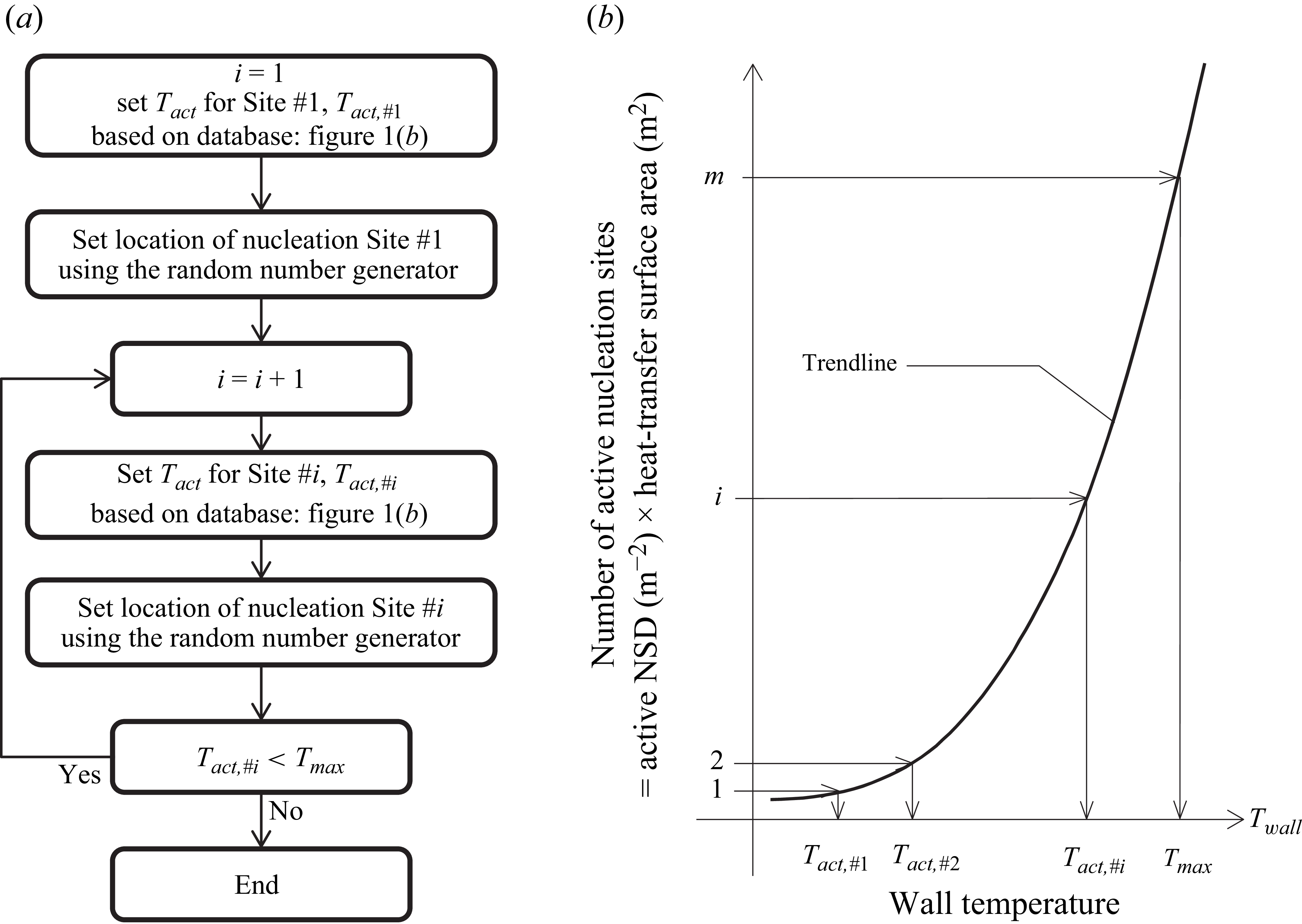

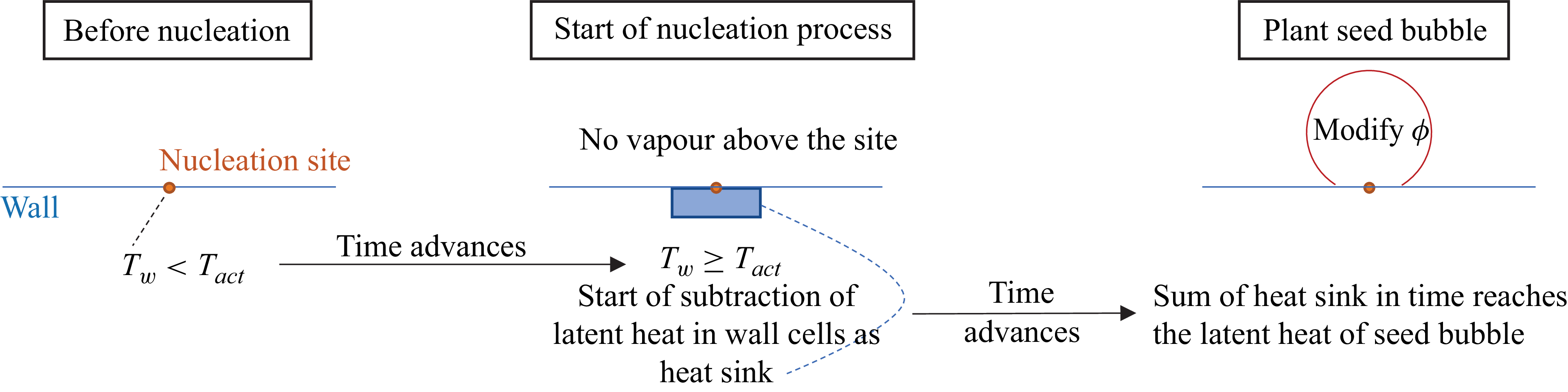
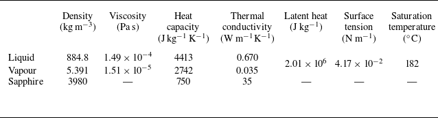


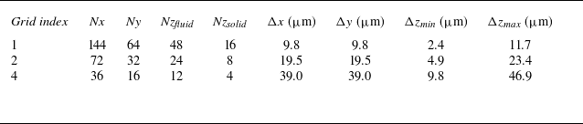
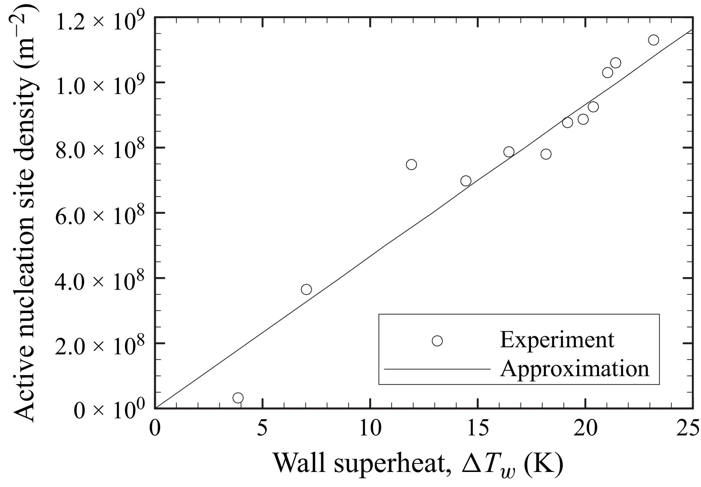

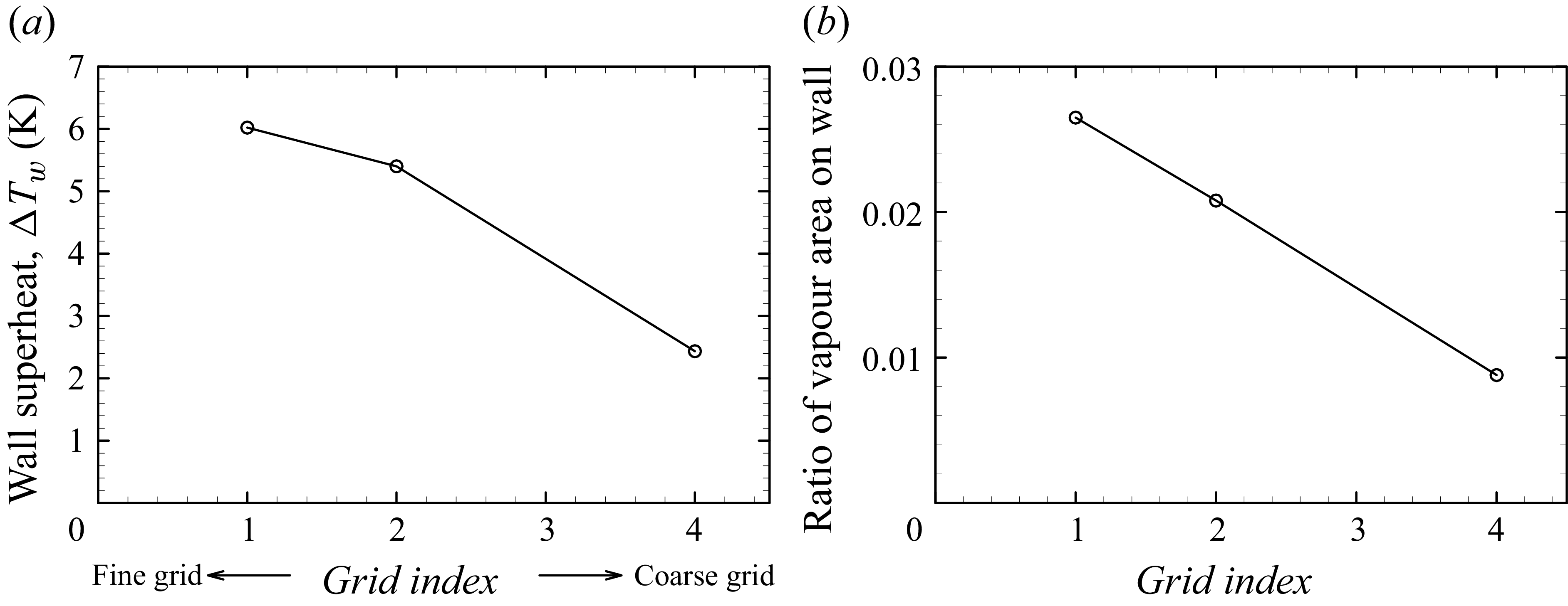


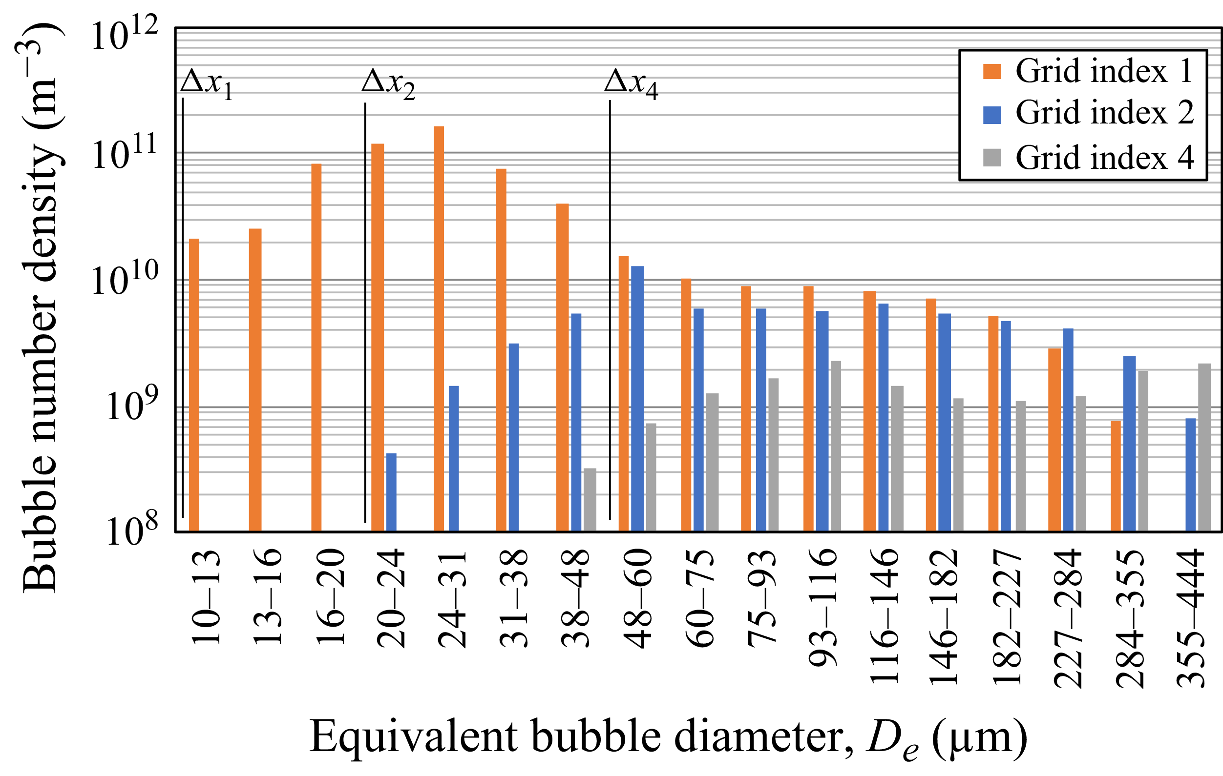
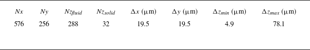


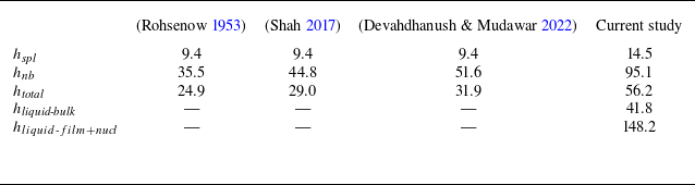


 Open access