





1. Introduction
Rheology aims to predict the complex flows of viscoelastic fluids using balance equations, equations of state (EOS) and constitutive equations. These equations can be solved once initial and boundary conditions are provided. While balance equations are universal, EOS and constitutive equations are system specific. Therefore, models for the EOS, relating temperature and pressure to mass and energy densities, and for the constitutive equations, relating stress and microstructural conformation tensors are required. The exact functional form of these models is generally unknown (Bird et al. Reference Bird, Bird, Armstrong and Hassager1987; de Pablo & Schieber Reference de Pablo and Schieber2014).
Traditionally, physical models are postulated based on physical intuition and are characterized by a small number of parameters that, ideally, can identify physical constants and material properties (Dyson Reference Dyson2004). In particular, rheologists have dedicated huge efforts to find good models that describe complex flow properties and behaviour (Oldroyd & Wilson Reference Oldroyd and Wilson1950; Thien & Tanner Reference Thien and Tanner1977; Larson Reference Larson1988; Herrchen & Öttinger Reference Herrchen and Öttinger1997; Kröger Reference Kröger2010). Once a model is proposed, model parameters are typically determined through simple experiments (i.e. in rheology shear or extensional steady-state viscometric flows). These experiments are designed to fit or ‘learn’ the model’s parameters in order to achieve good predictions. Models with a minimal number of parameters enable their determination with a limited amount of data from a few simple flow experiments involving shear or extensional steady-state viscometric flows. A fundamental problem in rheology is whether viscometric flow experiments are sufficient to obtain the parameters of a model to be applied in complex flow situations. A good physical model should describe a wide range of flow situations beyond those used to fit the parameters. However, there is no guarantee that a model performing well in simple flows will excel in complex flow situations. When the model fails, it must either be improved or replaced by a new one that incorporates additional physical insight. This process often entails identifying key physical features, such as finite extensibility, constraints imposed by entanglements, etc., that better capture the system’s behaviour. The systematic process of model refinement by including new physics, however, might be time-consuming, and we may also end up with something that looks very different to a good physical model with a small number of parameters (Dyson Reference Dyson2004).
An alternative, is to use a model with a sufficiently large number of parameters to fit the elephant (Dyson Reference Dyson2004). We lose the physical intuition concerning the behaviour of the model but, provided that a sufficiently large amount of data are available, we may automatize the entire process. Thanks to the universal approximation theorem (Hornik, Stinchcombe & White Reference Hornik, Stinchcombe and White1989), we may use a neural network (NN) to represent the functional form of a model with enough flexibility. The model is given by the composition of functions with very simple functional forms (like sigmoidal functions), resulting in a generic functional form depending on a large number of parameters. Using NN as the model, we may fit its parameters (train the network) in any region of the space of variables, be it the region of viscometric flows, or in arbitrary regions of complex flows. This allows us to simply retrain the NN model with new information when we require predictions for flow simulations of increasing complexity. Graphically, we hammer the function against data as a blacksmith would hammer a sheet of metal to shape it.
Traditional NNs have been used in multiscale simulation methods to retain the microscopic molecular fidelity at the macroscale (Lei, Wu & Weinan Reference Lei, Wu and E2020). Neural networks, while powerful function approximators, often disregard established constitutive modelling principles and thermodynamic constraints. As any interpolation method, NNs will give good predictions in the vicinity of training points and will fail extrapolating to regions far from their training data (Bonfanti et al. Reference Bonfanti, Santana, Ellero and Gholami2023, Reference Bonfanti, Bruno and Cipriani2024). Furthermore, NNs typically require large data sets to achieve a decent training (Rackauckas et al. Reference Rackauckas, Ma, Martensen, Warner, Zubov, Supekar, Skinner, Ramadhan and Edelman2021). In the context of rheology, data-driven approaches have been used to model nonlinear viscoelastic materials at small strains using NNs, requiring only stress and strain paths for training. These NNs can be tuned to satisfy some physical feature (i.e. convexity of the learned functional) to facilitate the handling of large data sets and noisy stress data (Rosenkranz et al. Reference Rosenkranz, Kalina, Brummund, Sun and Kästner2024).
Several lines of research aim at leveraging the potential advantages of machine learning methodologies in the field of rheology. Young et al. have employed scattering microstructure data to develop low dimensional constitutive models using a dimensionality reduction scheme (Young et al. Reference Young, Corona, Datta, Helgeson and Graham2023). Zhao and coworkers have employed yet a different machine learning methodology – Gaussian process regression – to learn constitutive models from microscopic simulations under simple shear flows. These constitutive models can then be used in macroscopic simulations (Zhao et al. Reference Zhao, Li, Caswell, Ouyang and Karniadakis2018, Reference Zhao, Li, Wang, Caswell, Ouyang and Karniadakis2021). However, an important limitation of these studies is that they set arbitrary constraints to the functional form of the learned rheological model. For example, setting the viscosity as function of shear rate alone (Zhao et al. Reference Zhao, Li, Caswell, Ouyang and Karniadakis2018) or, having the microstructure description relying on a predefined FENE-P model to incorporate viscoelasticity (Zhao et al. Reference Zhao, Li, Wang, Caswell, Ouyang and Karniadakis2021), thus these approaches lack generality. A more general, yet similar in the ad hoc choice of the functional form of the constitutive model is the work by Seryo et al. (Reference Seryo, Sato, Molina and Taniguchi2020). Gaussian process regression is also used to learn a constitutive model that introduces history-dependent viscoelasticity by considering the time derivative of the polymeric stress as a function of the flow velocity gradient and the stress (Seryo et al. Reference Seryo, Sato, Molina and Taniguchi2020). However, as the model becomes more general the dimensionality also tends to grow. For example in Seryo et al. work, the derivative of the stress ${\partial \boldsymbol \tau }/{\partial t}(\boldsymbol \nabla \boldsymbol v, \boldsymbol \tau )$
with a priori six independent components for three-dimensional (3-D) problems should be learned from the velocity gradient
${\partial \boldsymbol \tau }/{\partial t}(\boldsymbol \nabla \boldsymbol v, \boldsymbol \tau )$
with a priori six independent components for three-dimensional (3-D) problems should be learned from the velocity gradient $\boldsymbol \nabla \boldsymbol v$
with nine independent components and the symmetric stress
$\boldsymbol \nabla \boldsymbol v$
with nine independent components and the symmetric stress $\boldsymbol \tau$
with additional six independent components (i.e. mapping 15-dimensional space into six-dimensional space), making the approach difficult to apply in complex 3-D flows. A more effective, yet general, physics-informed dimensionality reduction is thus required to study complex 3-D flows.
$\boldsymbol \tau$
with additional six independent components (i.e. mapping 15-dimensional space into six-dimensional space), making the approach difficult to apply in complex 3-D flows. A more effective, yet general, physics-informed dimensionality reduction is thus required to study complex 3-D flows.
Another alternative is to utilize Physics-Informed NNs (PINNs) (Raissi, Perdikaris & Karniadakis Reference Raissi, Perdikaris and Karniadakis2019), a novel family of NNs which are able to inherently satisfy kinematic, thermodynamic and physical constraints (Linka & Kuhl Reference Linka and Kuhl2023). PINNs are NNs that incorporate model equations, such as partial differential equations (PDEs), directly into their structure. PINNs are currently employed to solve forward and inverse PDE problems (Raissi et al. Reference Raissi, Perdikaris and Karniadakis2019), fractional equations (Pang et al. Reference Pang, Lu and Karniadakis2019), integral–differential equations (Yuan et al. Reference Yuan, Ni, Deng and Hao2022) and stochastic PDEs (Zhang et al. Reference Zhang, Lu, Guo and Karniadakis2019). These innovative functions act as a multitask learning framework where the NN simultaneously fits observed data and minimizes the residual of the selected PDE (Cuomo et al. Reference Cuomo, Di Cola, Giampaolo, Rozza, Raissi and Piccialli2022; Mahmoudabadbozchelou et al. 2022b). The introduction of governing equations in the loss function enables PINNs to offer a powerful framework for solving forward and inverse problems in fluid mechanics, where the solutions to momentum balance equations that incorporate complex constitutive models are produced as predictions of the NN (Karniadakis et al. Reference Karniadakis, Kevrekidis, Lu, Perdikaris, Wang and Yang2021). However, most of the studies using PINNs have focused on predictions of specific flow simulations (i.e. using the network to solve momentum balance equations) and then choose the right constitutive model from a selection of ‘known’ analytical constitutive models rather than learning ‘unknown’ constitutive models (Meng et al. Reference Meng, Li, Zhang and Karniadakis2020; Lin et al. Reference Lin, Mao, Wang and Karniadakis2023). For example, Thakur et al. used PINNs to select among several viscoelastic constitutive models (Oldroyd-B (OB), Giesekus or linear PTT) and learn the stress field from a velocity field (Thakur, Raissi & Ardekani Reference Thakur, Raissi and Ardekani2022). In Saadat, Mahmoudabadbozchelou & Jamali (Reference Saadat, Mahmoudabadbozchelou and Jamali2022) and Mahmoudabadbozchelou et al. (Reference Mahmoudabadbozchelou, Kamani, Rogers and Jamali2022a ), the authors have proposed the rheology-informed NNs (RhINNs) for forward and inverse metamodelling of complex fluids. The RhINNs are employed to solve the constitutive models with multiple ordinary differential equations by proposing a penalization based on a thixoviscoelastoplastic model for the stress, where a few model parameters are learnt. Again, the framework used to encapsulate the physics is over-restricting for general complex fluids.
Nevertheless, PINNs present a significant advantage over traditional data-driven models by ensuring that the NN solutions adhere to fundamental physical principles. This feature is particularly beneficial in the context of rheology, where the complexity of the flow behaviour demands models that respect the underlying physics while adapting to diverse and nonlinear phenomena. In this context a number of studies have employed PINNs to advance rheological modelling. An interesting use regarding the problem discussed above is to employ PINNs to model viscoelastic materials using deep NNs to approximate rate-dependent and nonlinear constitutive relationships (Xu et al. Reference Xu, Tartakovsky, Burghardt and Darve2021). One way to impose a minimal set of thermodynamics-based constraints (i.e. first and second laws of thermodynamics) on constitutive models, still retaining generality, is through the application of the so-called GENERIC (General Equations of Non-Equilibrium Reversible–Irreversible Coupling) framework (Ottinger Reference Ottinger2005). Hernandez et al. proposed structure-preserving NNs (Hernández et al. Reference Hernández, Badías, González, Chinesta and Cueto2021). Zhang et al. proposed a GENERIC formalism informed NNs (GFINNs) that adhere to the formalism symmetric degeneracy conditions. GFINNs consist of two modules, each with two components, modelled by NNs specifically designed to meet these conditions. This componentwise architecture allows flexible integration of physical information into the networks (Zhang et al. Reference Zhang, Shin and Em Karniadakis2022).
In this work, we present a general approach for polymer solutions using PINNs to determine the polymeric entropy leading to the constitutive equation for the stress in rheological models. Instead of training PINNs to predict arbitrary solutions of specific flow simulations, we aim to leverage their universal approximator nature to capture the general functional relation between the eigenvalues of the conformation tensor $\boldsymbol c$
and the polymeric entropy for ‘a priori’ unknown viscoelastic models. The approach is not only GENERIC-compliant but also significantly reduces the problem dimensionality making model learning more efficient. In fact, it only requires learning a scalar state function (the entropy) as a function of the two or three eigenvalues (depending on space dimension) of the conformation tensor
$\boldsymbol c$
and the polymeric entropy for ‘a priori’ unknown viscoelastic models. The approach is not only GENERIC-compliant but also significantly reduces the problem dimensionality making model learning more efficient. In fact, it only requires learning a scalar state function (the entropy) as a function of the two or three eigenvalues (depending on space dimension) of the conformation tensor $\boldsymbol c$
. We evaluate the traditional methods using limited regions of the available conformation space (i.e. limited data from steady-state rheometric flows) to establish rheological models that then can be used to predict properties and behaviour of more complex flows. We propose two types of data sets to train our PINN models: a first one – in analogy to classical rheological calibrations – with steady-state rheometric flows (later denoted as ‘PINN-rheometric’); and a second one, with data from steady-state solutions of complex flow around a cylinder (later denoted as ‘PINN-complex’). We study the application of the PINN models to finite volume (FV) simulations of complex flows coupling the learned models with an OpenFOAMs RheoTool solver (Alves, Pinho & Oliveira Reference Alves, Pinho and Oliveira2001; Pimenta & Alves Reference Pimenta and Alves2017). We find that a PINN model trained in steady-state rheometric flows data can be used to produce reasonable predictions in moderate transient or complex flows. However, in order to reproduce complex flows more accurately, data retrieved beyond viscometric flows are required for training.
$\boldsymbol c$
. We evaluate the traditional methods using limited regions of the available conformation space (i.e. limited data from steady-state rheometric flows) to establish rheological models that then can be used to predict properties and behaviour of more complex flows. We propose two types of data sets to train our PINN models: a first one – in analogy to classical rheological calibrations – with steady-state rheometric flows (later denoted as ‘PINN-rheometric’); and a second one, with data from steady-state solutions of complex flow around a cylinder (later denoted as ‘PINN-complex’). We study the application of the PINN models to finite volume (FV) simulations of complex flows coupling the learned models with an OpenFOAMs RheoTool solver (Alves, Pinho & Oliveira Reference Alves, Pinho and Oliveira2001; Pimenta & Alves Reference Pimenta and Alves2017). We find that a PINN model trained in steady-state rheometric flows data can be used to produce reasonable predictions in moderate transient or complex flows. However, in order to reproduce complex flows more accurately, data retrieved beyond viscometric flows are required for training.
In order to evaluate the quality of the PINN model predictions, we analyse the relative errors of the entropy and the stress in the space of the eigenvalues of $\boldsymbol c$
. We generate in silico conformation-tensor data according to analytical and accurate RheoTool-discretizations of an OB model in simple and complex flows. Data are provided to the PINN for training, whereas its application to complex flow is agnostic of the underlying model used to generate them, therefore providing an optimal and controlled framework for fair numerical comparisons. The PINN model presented here can effectively learn unknown forms of the polymeric entropy and integrate their GENERIC-guided NN representation into RheoTool to perform data-driven flow simulations. The only data required to train these models are the conformation tensor and velocities fields in complex flow. These kind of datasets can be obtained, for example, in experiments through combined use of particle image velocimetry and flow-induced birefringence measurements (Haward et al. Reference Haward, Hopkins, Varchanis and Shen2021), X-ray scattering measurements (Mao, McCready & Burghardt Reference Mao, McCready and Burghardt2014; McCready & Burghardt Reference McCready and Burghardt2015) or, in the case of multiscale applications, from independent mesoscale polymer computations (Simavilla & Ellero Reference Nieto Simavilla and Ellero2022; Simavilla et al. Reference Nieto Simavilla, Español and Ellero2023). Thus, we aim to leverage the potential of PINNs to provide rheologists with more effective, thermodynamics-guided ways to discover constitutive equations from data and, at the same time, applying them directly to fluid mechanics simulations using CFD.
$\boldsymbol c$
. We generate in silico conformation-tensor data according to analytical and accurate RheoTool-discretizations of an OB model in simple and complex flows. Data are provided to the PINN for training, whereas its application to complex flow is agnostic of the underlying model used to generate them, therefore providing an optimal and controlled framework for fair numerical comparisons. The PINN model presented here can effectively learn unknown forms of the polymeric entropy and integrate their GENERIC-guided NN representation into RheoTool to perform data-driven flow simulations. The only data required to train these models are the conformation tensor and velocities fields in complex flow. These kind of datasets can be obtained, for example, in experiments through combined use of particle image velocimetry and flow-induced birefringence measurements (Haward et al. Reference Haward, Hopkins, Varchanis and Shen2021), X-ray scattering measurements (Mao, McCready & Burghardt Reference Mao, McCready and Burghardt2014; McCready & Burghardt Reference McCready and Burghardt2015) or, in the case of multiscale applications, from independent mesoscale polymer computations (Simavilla & Ellero Reference Nieto Simavilla and Ellero2022; Simavilla et al. Reference Nieto Simavilla, Español and Ellero2023). Thus, we aim to leverage the potential of PINNs to provide rheologists with more effective, thermodynamics-guided ways to discover constitutive equations from data and, at the same time, applying them directly to fluid mechanics simulations using CFD.
2. Methods
2.1. The GENERIC-guided approach to model constitutive equations
In the present work, we are interested in the modelling of polymeric solutions. Within the GENERIC framework, a general polymer model can be cast into a set of PDEs including the mass and momentum balance equations
 \begin{align} &\qquad\qquad\qquad\qquad\qquad\quad \boldsymbol{\nabla } \cdot \boldsymbol{v} = 0 ,\end{align}
 \begin{align} &\rho \left (\frac{\partial \boldsymbol{v}}{\partial t} + \boldsymbol{v} \cdot \nabla \boldsymbol{v}\right ) - \nabla \cdot \left(\frac{\eta _s}{2} \big(\nabla \boldsymbol{v} + \nabla \boldsymbol{v}^T \big) \right) = -\nabla p + \nabla \cdot \boldsymbol{\tau } ,\end{align}
where $\boldsymbol{v}$
is the velocity vector field,
$\boldsymbol{v}$
is the velocity vector field, $p$
is the pressure and
$p$
is the pressure and $\boldsymbol \tau$
is the non-Newtonian extra-stress term coupled with an evolution equation for the conformation tensor
$\boldsymbol \tau$
is the non-Newtonian extra-stress term coupled with an evolution equation for the conformation tensor $\boldsymbol c$
, which represents the microstructure generated by the polymers (Ottinger Reference Ottinger2005). For a polymer solution undergoing affine deformation, the conformation tensor generally evolves according to (Vázquez-Quesada et al. Reference Vázquez-Quesada, Ellero and Español2009b
; Simavilla et al. Reference Nieto Simavilla, Español and Ellero2023)
$\boldsymbol c$
, which represents the microstructure generated by the polymers (Ottinger Reference Ottinger2005). For a polymer solution undergoing affine deformation, the conformation tensor generally evolves according to (Vázquez-Quesada et al. Reference Vázquez-Quesada, Ellero and Español2009b
; Simavilla et al. Reference Nieto Simavilla, Español and Ellero2023)
 \begin{align} \partial _t {\boldsymbol c} = - {\boldsymbol v} \cdot {\boldsymbol \nabla } {\boldsymbol c} + {\boldsymbol c}\cdot \boldsymbol{\kappa } + \boldsymbol{\kappa }^T \cdot {\boldsymbol c} +\frac {2}{\lambda _{ {p}} n_{{p}} k_BT}{\boldsymbol c}\cdot {\boldsymbol {\sigma }}, \end{align}
where $\lambda _{{p}}$
is the polymeric characteristic relaxation time,
$\lambda _{{p}}$
is the polymeric characteristic relaxation time, $n_{{p}}$
the polymer number density (i.e. the number of chains per unit volume),
$n_{{p}}$
the polymer number density (i.e. the number of chains per unit volume), $k_{{B}}$
is the Boltzmann constant and
$k_{{B}}$
is the Boltzmann constant and $T$
the temperature. The first three terms in (2.3) are reversible in nature, describing the kinematic evolution of the conformation tensor under the influence of the velocity gradient
$T$
the temperature. The first three terms in (2.3) are reversible in nature, describing the kinematic evolution of the conformation tensor under the influence of the velocity gradient $\boldsymbol{\kappa }=\nabla \boldsymbol{v}^T$
. The application of (2.3) is limited to dilute polymeric solutions where the fluid can be considered a suspension of non-interacting polymers. In GENERIC, the most general formulation of the governing equations where the polymer contributions are given by the conformation tensor takes the form (Ottinger Reference Ottinger2005)
$\boldsymbol{\kappa }=\nabla \boldsymbol{v}^T$
. The application of (2.3) is limited to dilute polymeric solutions where the fluid can be considered a suspension of non-interacting polymers. In GENERIC, the most general formulation of the governing equations where the polymer contributions are given by the conformation tensor takes the form (Ottinger Reference Ottinger2005)
 \begin{align} \partial _t {\boldsymbol c} = - {\boldsymbol v} \cdot {\boldsymbol \nabla } {\boldsymbol c} + {\boldsymbol c}\cdot \boldsymbol{\kappa } + \boldsymbol{\kappa }^T\cdot {\boldsymbol c} + \boldsymbol R_2 : \rho {\boldsymbol{\sigma }}, \end{align}
where $\boldsymbol R_2$
is a fourth-order tensor connected to the dissipation or friction matrix. In the scope of this manuscript we will focus on dilute polymeric solutions. For this kind of system, it has been shown (Vázquez-Quesada et al. Reference Vázquez-Quesada, Ellero and Español2009a
), that the Wiener process leads to
$\boldsymbol R_2$
is a fourth-order tensor connected to the dissipation or friction matrix. In the scope of this manuscript we will focus on dilute polymeric solutions. For this kind of system, it has been shown (Vázquez-Quesada et al. Reference Vázquez-Quesada, Ellero and Español2009a
), that the Wiener process leads to $\boldsymbol R_2 \propto \boldsymbol c$
and therefore (2.3). There are a number of ‘entropy’ models that are typically used for dilute suspensions of non-hydrodynamically interacting polymers where the evolution of the conformation tensor is well represented by this equation (Ottinger Reference Ottinger2005). Learning general anisotropic models for concentrated systems requires determining
$\boldsymbol R_2 \propto \boldsymbol c$
and therefore (2.3). There are a number of ‘entropy’ models that are typically used for dilute suspensions of non-hydrodynamically interacting polymers where the evolution of the conformation tensor is well represented by this equation (Ottinger Reference Ottinger2005). Learning general anisotropic models for concentrated systems requires determining $\boldsymbol{R}_2(\boldsymbol{c})$
, which in turn necessitates incorporating additional physical information or data.
$\boldsymbol{R}_2(\boldsymbol{c})$
, which in turn necessitates incorporating additional physical information or data.
The last term in (2.3) describes the general irreversible evolution of the conformation tensor. This term is characterized by the thermodynamic force ${\boldsymbol \sigma }({\boldsymbol c})$
, defined as the derivative of the polymeric entropy density
${\boldsymbol \sigma }({\boldsymbol c})$
, defined as the derivative of the polymeric entropy density $s_{{p}}({\boldsymbol c})$
with respect to the conformation tensor
$s_{{p}}({\boldsymbol c})$
with respect to the conformation tensor $\boldsymbol c$
, that is
$\boldsymbol c$
, that is
 \begin{align} \frac {\boldsymbol \sigma }{T}=\frac {\partial s_{{p}}}{\partial \boldsymbol c}. \end{align}
Finally, the momentum balance equation contains, in addition to the solvent viscous stress, a polymeric stress given by (Vázquez-Quesada et al. Reference Vázquez-Quesada, Ellero and Español2009b )
 \begin{align} \boldsymbol \tau = - 2 \boldsymbol c \cdot \boldsymbol \sigma \end{align}
which satisfies the dynamics–thermodynamics compatibility (i.e. consistency with the microstructural evolution given by (2.3)). Therefore, the knowledge of the entropy function directly provides the closure in a thermodynamic-consistent constitutive equation for a dilute polymeric suspension.
Since the entropy is invariant under rotations, it can only depend on the invariants of the conformation tensor $\boldsymbol c$
, that we choose to be the eigenvalues
$\boldsymbol c$
, that we choose to be the eigenvalues $c_1,c_2,c_3$
and therefore,
$c_1,c_2,c_3$
and therefore, $s_{{p}}({\boldsymbol c})=s_{{p}}(c_1,c_2,c_3)$
. Observe that the tensors
$s_{{p}}({\boldsymbol c})=s_{{p}}(c_1,c_2,c_3)$
. Observe that the tensors $\boldsymbol c$
and
$\boldsymbol c$
and $\boldsymbol \sigma$
commute (Vázquez-Quesada et al. Reference Vázquez-Quesada, Ellero and Español2009b
) and diagonalize simultaneously. This implies that we may write (2.5) as
$\boldsymbol \sigma$
commute (Vázquez-Quesada et al. Reference Vázquez-Quesada, Ellero and Español2009b
) and diagonalize simultaneously. This implies that we may write (2.5) as
 \begin{align} \frac {\sigma _\alpha }{T}=\frac {\partial s_{{p}}}{\partial c_\alpha }, \end{align}
where $\sigma _\alpha (\alpha =1,..,D$
) are the eigenvalues of
$\sigma _\alpha (\alpha =1,..,D$
) are the eigenvalues of ${\boldsymbol{\sigma }}$
. Because of the large reduction of arguments of the entropy due to rotational symmetry, it proves convenient to express the dynamics in terms of eigenvalues and eigenvectors. The decomposition of (2.3) into eigenvalues and eigenvectors (i.e.
${\boldsymbol{\sigma }}$
. Because of the large reduction of arguments of the entropy due to rotational symmetry, it proves convenient to express the dynamics in terms of eigenvalues and eigenvectors. The decomposition of (2.3) into eigenvalues and eigenvectors (i.e. $\boldsymbol{c}=\sum _\alpha c_\alpha {\boldsymbol u}_\alpha {\boldsymbol u}_\alpha ^{\textrm{T}}$
) leads to two coupled PDEs (Vázquez-Quesada et al. Reference Vázquez-Quesada, Ellero and Español2009b
),
$\boldsymbol{c}=\sum _\alpha c_\alpha {\boldsymbol u}_\alpha {\boldsymbol u}_\alpha ^{\textrm{T}}$
) leads to two coupled PDEs (Vázquez-Quesada et al. Reference Vázquez-Quesada, Ellero and Español2009b
),
 \begin{align} 0 &= \partial _t c_{\alpha } + v_j\partial _jc_{\alpha } -2c_{\alpha }\kappa _{\alpha \alpha } - \frac {1}{\lambda _{{p}} n_{{p}} k_{{B}} T} c_\alpha \sigma _\alpha, \end{align}
 \begin{align} 0 &= \partial _t \boldsymbol u_{\alpha } + v_j\partial _j\boldsymbol u_{\alpha } - \sum _{\beta } H_{\alpha \beta }^{\textrm { }} \boldsymbol u_{\beta }, \end{align}
where $\kappa _{\alpha \alpha }=\boldsymbol{u}_\alpha \cdot \boldsymbol{\kappa }\cdot \boldsymbol{u}_\alpha$
is the velocity gradient in the eigenbasis of the conformation tensor, and the antisymmetric matrix
$\kappa _{\alpha \alpha }=\boldsymbol{u}_\alpha \cdot \boldsymbol{\kappa }\cdot \boldsymbol{u}_\alpha$
is the velocity gradient in the eigenbasis of the conformation tensor, and the antisymmetric matrix $H_{\alpha \beta }^{\textrm { }}$
is given by
$H_{\alpha \beta }^{\textrm { }}$
is given by
 \begin{align} H_{\alpha \beta }^{\textrm { }} = \frac {1}{c_\alpha -c_\beta }(c_\alpha \kappa _{\alpha \beta } + c_\beta \kappa _{\beta \alpha }). \end{align}
The kinematics of the flow in (2.9) has been used by the authors in Simavilla et al. (Reference Nieto Simavilla, Español and Ellero2023) to establish the non-affine characteristics of polymer flow by introducing a mixed derivative of the Gordon–Schowalter type. This allows for the unambiguous separation of reversible/irreversible terms in the dynamics, enabling to split non-Newtonian effects related to non-affine deformation, with irreversible effects intrinsically associated with the polymeric entropy $s_p(\textbf {c})$
, which is crucial to apply safely the model to arbitrary flows. For simplicity, non-affine motion is not considered here as it will be the subject of future refinements of the methodology. Note that the entropy appears only in (2.8) through
$s_p(\textbf {c})$
, which is crucial to apply safely the model to arbitrary flows. For simplicity, non-affine motion is not considered here as it will be the subject of future refinements of the methodology. Note that the entropy appears only in (2.8) through $\sigma _\alpha$
. Equation (2.8) will be used below to construct the residuals and the loss function in the PINN model.
$\sigma _\alpha$
. Equation (2.8) will be used below to construct the residuals and the loss function in the PINN model.
In this paper, we address the following problem: given that the dynamics of the polymer solution are described by (2.3) or its equivalent, (2.8), and that we have explicit data for the fields ${\boldsymbol v}(\boldsymbol{r},t)$
and
${\boldsymbol v}(\boldsymbol{r},t)$
and ${\boldsymbol c}(\boldsymbol{r},t)$
, our objective is to develop a Physics-Informed NN (PINN) representation of the specific entropy function
${\boldsymbol c}(\boldsymbol{r},t)$
, our objective is to develop a Physics-Informed NN (PINN) representation of the specific entropy function $s_p(\textbf{c})$
. This PINN model should ensure that the measured fields align with the governing equation (2.3) dictated by GENERIC. It should be also noticed that our approach diverges from the usual application of PINNs where the NNs represent the fields
$s_p(\textbf{c})$
. This PINN model should ensure that the measured fields align with the governing equation (2.3) dictated by GENERIC. It should be also noticed that our approach diverges from the usual application of PINNs where the NNs represent the fields ${\boldsymbol v}(\boldsymbol{r},t)$
and
${\boldsymbol v}(\boldsymbol{r},t)$
and ${\boldsymbol c}(\boldsymbol{r},t)$
directly (Karniadakis et al. Reference Karniadakis, Kevrekidis, Lu, Perdikaris, Wang and Yang2021). In contrast, in this paper, we focus solely on employing a single NN to model the functional form of the entropy. From this knowledge alone,
${\boldsymbol c}(\boldsymbol{r},t)$
directly (Karniadakis et al. Reference Karniadakis, Kevrekidis, Lu, Perdikaris, Wang and Yang2021). In contrast, in this paper, we focus solely on employing a single NN to model the functional form of the entropy. From this knowledge alone, $s_{{p}}$
can be used to provide all the necessary stress predictions in CFD simulations (i.e. using RheoTool).
$s_{{p}}$
can be used to provide all the necessary stress predictions in CFD simulations (i.e. using RheoTool).
2.2. The NN
To demonstrate the methodology, this paper focuses on two-dimensional (2-D) flows, with the extension to 3-D flows being straightforward. We aim at representing the functional form of the entropy $s_{{ p}}(\mathsf{C}):\mathbb{R}^2\to \mathbb{R}$
as a function of the eigenvalues
$s_{{ p}}(\mathsf{C}):\mathbb{R}^2\to \mathbb{R}$
as a function of the eigenvalues $\mathsf{C}=\{c_1,c_2\}\in \mathbb{R}^2$
through a NN of the form
$\mathsf{C}=\{c_1,c_2\}\in \mathbb{R}^2$
through a NN of the form
 \begin{align} \tilde s_{{p}}(\mathsf{C})= n_{{p}} k_B \tilde s_\theta (\mathsf{C}) \end{align}
where $n_{{p}}$
is the polymer number density and the dimensionless NN is
$n_{{p}}$
is the polymer number density and the dimensionless NN is
 \begin{align} \tilde s_\theta (\mathsf{C})=\big[ W_L\cdot \phi ( \cdots \phi (W_1 \cdot \phi (W_0 \mathsf{C}+b_0)+b_1 )\cdots ) + b_L\big](\mathsf{C}-\mathsf{C}_{{ eq}})^2 \end{align}
where $W_k \in \mathbb{R}^{h_k\times h_{k-1}}$
and
$W_k \in \mathbb{R}^{h_k\times h_{k-1}}$
and $b_k\in \mathbb{R}^{h_k}$
denote, respectively, the weights and biases of the
$b_k\in \mathbb{R}^{h_k}$
denote, respectively, the weights and biases of the $k$
th hidden layer, with
$k$
th hidden layer, with $k\in (0,\cdots ,L)$
. The number of nodes of the
$k\in (0,\cdots ,L)$
. The number of nodes of the $k$
th layer is
$k$
th layer is $h_k$
. The collection of all trainable parameters of the network is identified as
$h_k$
. The collection of all trainable parameters of the network is identified as $\theta = \{W_k,b_k\}_{k=0}^L$
. The activation function
$\theta = \{W_k,b_k\}_{k=0}^L$
. The activation function $\phi : \mathbb{R} \to \mathbb{R}$
is a smooth nonlinear function that is applied elementwise to a multivariate argument. The choice of the function is arbitrary and often problem-dependent, with common selections for
$\phi : \mathbb{R} \to \mathbb{R}$
is a smooth nonlinear function that is applied elementwise to a multivariate argument. The choice of the function is arbitrary and often problem-dependent, with common selections for $\phi$
including the hyperbolic tangent or the sine function, chosen in this work. Finally, the factor involving the equilibrium value
$\phi$
including the hyperbolic tangent or the sine function, chosen in this work. Finally, the factor involving the equilibrium value $\mathsf{C}_{eq}=\{1,1\}$
of the conformation tensor’s eigenvalues is a common approach followed when implementing PINNs in order to impose exact satisfaction of boundary and/or initial conditions (Sukumar & Srivastava Reference Sukumar and Srivastava2022; Arzani, Cassel & D’Souza Reference Arzani, Cassel and D’Souza2023). In particular, we ensure that
$\mathsf{C}_{eq}=\{1,1\}$
of the conformation tensor’s eigenvalues is a common approach followed when implementing PINNs in order to impose exact satisfaction of boundary and/or initial conditions (Sukumar & Srivastava Reference Sukumar and Srivastava2022; Arzani, Cassel & D’Souza Reference Arzani, Cassel and D’Souza2023). In particular, we ensure that $s_{{p}}(\mathsf{C}_{{ eq}})=0$
and
$s_{{p}}(\mathsf{C}_{{ eq}})=0$
and ${\sigma }_\alpha (\mathsf{C}_{{ eq}})=\{0,0\}$
. This requirement is necessary because a non-zero entropy at the equilibrium will often result in unstable flow predictions once the NN is coupled with RheoTool. Additional information on the expressions for
${\sigma }_\alpha (\mathsf{C}_{{ eq}})=\{0,0\}$
. This requirement is necessary because a non-zero entropy at the equilibrium will often result in unstable flow predictions once the NN is coupled with RheoTool. Additional information on the expressions for $s_{{p}}$
, and therefore
$s_{{p}}$
, and therefore $\boldsymbol \sigma$
, for simple models are discussed in Appendix A.3.
$\boldsymbol \sigma$
, for simple models are discussed in Appendix A.3.
A graphical description of (2.12) is shown in figure 1, where it is also indicated how the eigenvalues $\sigma _\alpha$
are obtained from automatic differentiation of the NN entropy function with respect to
$\sigma _\alpha$
are obtained from automatic differentiation of the NN entropy function with respect to $\mathsf{C}$
.
$\mathsf{C}$
.
Sketch of the PINNs architecture.

The final ingredient of a NN is the loss function whose minimization produces the parameters of the network. The loss function in PINNs is constructed in terms of residuals of the PDE. The definition of the residuals $e_\alpha (c_\alpha ;\theta )$
follows from the GENERIC-consistent PDE (2.8) that already uses the NN representation in (2.11),
$e_\alpha (c_\alpha ;\theta )$
follows from the GENERIC-consistent PDE (2.8) that already uses the NN representation in (2.11),
 \begin{align} e_\alpha (c_\alpha ;\theta ) &\equiv \partial _t c_{\alpha } + v_j\partial _jc_{\alpha } -2c_{\alpha }\kappa _{\alpha \alpha } - \frac {2}{\lambda _{{p}} } c_\alpha \frac {\partial \tilde s_\theta }{\partial c_\alpha }, \end{align}
where $\alpha = 1,2$
for 2-D problems and the partial derivative of the NN
$\alpha = 1,2$
for 2-D problems and the partial derivative of the NN $\tilde s_\theta$
is computed through automatic differentiation (Paszke et al. Reference Paszke, Gross, Chintala, Chanan, Yang, DeVito, Lin, Desmaison, Antiga and Lerer2017). The residuals in (2.13) can be obtained through any dataset – produced either by simulation or experiments – for the velocity gradient and the microstructure (i.e. the conformation tensor).
$\tilde s_\theta$
is computed through automatic differentiation (Paszke et al. Reference Paszke, Gross, Chintala, Chanan, Yang, DeVito, Lin, Desmaison, Antiga and Lerer2017). The residuals in (2.13) can be obtained through any dataset – produced either by simulation or experiments – for the velocity gradient and the microstructure (i.e. the conformation tensor).
The residuals can be further simplified when the model is trained exclusively on the steady state line. Therefore, when training the PINN with synthetic viscometric data (PINN-rheometric), we will use the residual
 \begin{align} e_\alpha (c_\alpha ;\theta ) = -2c_{\alpha }\kappa _{\alpha \alpha } - \frac {2}{\lambda _{{p}}} c_\alpha \frac {\partial \tilde s_{\theta }}{\partial c_\alpha }. \end{align}
With either of the residuals defined by (2.13) and (2.14), we define the loss function
 \begin{align} \mathcal{L} \big(c_1 ^i, c_2 ^i, \theta \big) = \frac {1}{N}\sum _{i=1}^N \Bigl ( \lambda _1|| {e}_{1}\big(c_1 ^i;\theta \big) ||^2 + \lambda _2|| {e}_{2}\big(c_2 ^i;\theta \big) ||^2 \Bigr ) \end{align}
where $\{(c_1 ^i, c_2 ^i)\}_{i=1}^N$
represents the dataset with
$\{(c_1 ^i, c_2 ^i)\}_{i=1}^N$
represents the dataset with $N$
points used for the training of our model. The parameters
$N$
points used for the training of our model. The parameters $\lambda _1$
and
$\lambda _1$
and $\lambda _2$
represent two scalars whose purpose is to balance the interplay between the two residuals. Unbalanced loss components are known to be detrimental for the training process of PINNs, which can lead to slow or unfeasible convergence (Wang, Yu & Perdikaris Reference Wang, Yu and Perdikaris2022). We established the values of the two scalars based on the heuristics proposed in Schmid et al. (Reference Schmid, Bauerschmidt, Gurbuz, Eser and Marburg2024), where their value is given as the proportion of the two residuals at the first iteration. For the specific models we train in our study, we notice that this approach generally yields a ratio
$\lambda _2$
represent two scalars whose purpose is to balance the interplay between the two residuals. Unbalanced loss components are known to be detrimental for the training process of PINNs, which can lead to slow or unfeasible convergence (Wang, Yu & Perdikaris Reference Wang, Yu and Perdikaris2022). We established the values of the two scalars based on the heuristics proposed in Schmid et al. (Reference Schmid, Bauerschmidt, Gurbuz, Eser and Marburg2024), where their value is given as the proportion of the two residuals at the first iteration. For the specific models we train in our study, we notice that this approach generally yields a ratio $\lambda _1/\lambda _2 \approx 10^{-4}$
. Finally, by minimizing the loss function in (2.15), we identify the optimal NN entropy function that ensures the dynamic equations in (2.13) to be consistent with the data. We train our models by the Adam optimizer (Kingma & Ba Reference Kingma and Ba2014), which is an enhanced first-order stochastic optimization algorithm ubiquitous in the machine learning community.
$\lambda _1/\lambda _2 \approx 10^{-4}$
. Finally, by minimizing the loss function in (2.15), we identify the optimal NN entropy function that ensures the dynamic equations in (2.13) to be consistent with the data. We train our models by the Adam optimizer (Kingma & Ba Reference Kingma and Ba2014), which is an enhanced first-order stochastic optimization algorithm ubiquitous in the machine learning community.
One of the main benefits of using a PINN to approach the minimization of PDE residuals is the flexibility of the training formulation. Indeed, all the physical quantities included in (2.13) can be obtained through high-fidelity numerical simulation, or experimental measurements and all those data can be introduced in the same training scheme.
Flowchart of the procedure for macroscopic flow simulations using RheoTool and Python script PINN integration. Orange boxes refer to RheoTool actions. Purple boxes refer to actions in python script.

2.3. Data-driven CFD: coupling PINN with RheoTool
The macroscopic flow simulations in this article have been performed using the RheoTool library. RheoTool is an extension for OpenFOAM (FV), a popular open-source computational fluid dynamics (CFD) software, designed specifically for simulating non-Newtonian flows. The software RheoTool was developed by Pimenta et al. to provide advanced viscoelastic numerical methods to the OpenFOAM community (Pimenta & Alves Reference Pimenta and Alves2017). The software RheoTool is publicly available and incorporates various constitutive models for non-Newtonian fluids including power-law, Carreau, Cross, Bingham, Herschel–Bulkley and viscoelastic models like OB, Giesekus and FENE-P, among many others.
In this paper, we use a modification of the rheoFoam uncoupled solver that incorporates a python script where the PINN model is executed using PyTorch. The RheoTool-PINN interaction is achieved using the PythonPal interface (Rodriguez & Cardiff Reference Rodriguez and Cardiff2022), a header-only library that provides high-level methods for OpenFOAM (C++) to Python communication. For example, it provides ready-to-use methods such as the constructor for the python script, a passToPython function that creates a NumPy array in the Python interpreter from OpenFOAM data, and the execute command to run the python script. After initiating the PyTorch library and setting required variables in the modified solver, the following steps are executed at each time iteration (see the flowchart in figure 2). First, the continuity equation (2.1) and momentum equation (2.2) are solved using a SIMPLEC type iteration. The term $({\eta _s}/{2}) (\nabla \boldsymbol{v} + \nabla \boldsymbol{v}^T )$
represents the diffusive term of the solvent stress contribution, which is solved implicitly. In contrast,
$({\eta _s}/{2}) (\nabla \boldsymbol{v} + \nabla \boldsymbol{v}^T )$
represents the diffusive term of the solvent stress contribution, which is solved implicitly. In contrast, $\nabla \cdot \boldsymbol{\tau }$
is handled explicitly. The momentum equation is solved using RheoTool’s coupling both-sides-diffusion stabilization technique. After the SIMPLEC iteration on continuity and momentum equations is completed, the constitutive equation for the symmetric conformation tensor
$\nabla \cdot \boldsymbol{\tau }$
is handled explicitly. The momentum equation is solved using RheoTool’s coupling both-sides-diffusion stabilization technique. After the SIMPLEC iteration on continuity and momentum equations is completed, the constitutive equation for the symmetric conformation tensor $\boldsymbol{c}$
is solved in a semi-implicit form, where the right-hand side of the equation is solved explicitly,
$\boldsymbol{c}$
is solved in a semi-implicit form, where the right-hand side of the equation is solved explicitly,
 \begin{equation} \partial _t {\boldsymbol{c}} + \left ( \boldsymbol{v} \cdot \nabla \boldsymbol{c} \right ) = \big( \boldsymbol{c} \cdot \boldsymbol{\kappa } + \boldsymbol{\kappa }^T \cdot \boldsymbol{c}\big) + \frac {2}{\lambda _{{p}} n_{{p}} k_{{B}}T}\boldsymbol{c} \cdot {\boldsymbol{\sigma }}. \end{equation}
Next, a python script is executed which involves the following steps. First, the eigenvalues $\{c_1, c_2\}$
and normalized eigenvectors
$\{c_1, c_2\}$
and normalized eigenvectors $\{\boldsymbol{u}_1, \boldsymbol{u}_2\}$
of the conformation
$\{\boldsymbol{u}_1, \boldsymbol{u}_2\}$
of the conformation $\boldsymbol{c}$
are computed in each cell and sorted by size, where
$\boldsymbol{c}$
are computed in each cell and sorted by size, where $c_1 \gt c_2$
. Then,
$c_1 \gt c_2$
. Then, $\{\sigma _1, \sigma _2\}$
values in each cell are obtained through automatic differentiation of the PINN entropy representation computed from
$\{\sigma _1, \sigma _2\}$
values in each cell are obtained through automatic differentiation of the PINN entropy representation computed from $\{c_1, c_2\}$
. As a next step, conjugate variable
$\{c_1, c_2\}$
. As a next step, conjugate variable ${\boldsymbol{\sigma }}$
is reconstructed using the eigenvalues
${\boldsymbol{\sigma }}$
is reconstructed using the eigenvalues $\{\sigma _1, \sigma _2\}$
and eigenvectors
$\{\sigma _1, \sigma _2\}$
and eigenvectors $\{\boldsymbol{u}_1, \boldsymbol{u}_2\}$
as
$\{\boldsymbol{u}_1, \boldsymbol{u}_2\}$
as
 \begin{equation} {\boldsymbol{\sigma }}=\sum _\alpha \sigma _\alpha \boldsymbol{u}_\alpha \boldsymbol{u}_\alpha ^{T}. \end{equation}
Finally, the non-Newtonian extra-stress $\boldsymbol{\tau }$
is computed from (2.6) as
$\boldsymbol{\tau }$
is computed from (2.6) as
 \begin{align} \boldsymbol{\tau } = -\dfrac {2 \eta _p}{\lambda _{{p}} n_{{p}} k_{{B}} T}(\boldsymbol{c} \cdot \boldsymbol \sigma ) \end{align}
or equivalently
 \begin{align} \boldsymbol{\tau } = -\dfrac {\eta _p}{\lambda }\left(\boldsymbol{c} \cdot \frac {\partial \tilde s_\theta }{\partial \boldsymbol c}\right). \end{align}
The computed stress is then used back in the SIMPLEC iteration of RheoTool, closing the time step loop. A graphical sketch of the structure of the algorithm is shown in figure 2.
3. Numerical results
3.1. The PINN-rheometric: training
To validate the present methodology, we first use data produced by the analytical solution to (2.3) with (2.1), (2.2) in steady-state rheometric flows. We denominate the PINN trained with this dataset: PINN-rheometric. Since all steady-state rheometric flow solutions using the OB model fall on the same line in the $c_1$
–
$c_1$
– $c_2$
space, we choose to implement our training with data for the simplest analytical solution, i.e. steady-state extensional flow characterized by extensional rate
$c_2$
space, we choose to implement our training with data for the simplest analytical solution, i.e. steady-state extensional flow characterized by extensional rate $\dot {\epsilon }$
. For the OB the analytical expression for the entropy is given by (Ottinger Reference Ottinger2005)
$\dot {\epsilon }$
. For the OB the analytical expression for the entropy is given by (Ottinger Reference Ottinger2005)
 \begin{equation} s_{{p}}(c_1,c_2) = \frac {k_{{B}}}{2}(2 - c_1 - c_2 + \ln {c_1} + \ln {c_2}) \end{equation}
which represents the ground truth solution to target with data, whereas in extensional flow the eigenvalues of the conformation tensor $c_\alpha$
at a given Wi are
$c_\alpha$
at a given Wi are
 \begin{align} c_{1} = & \frac {1}{1-2\textit{Wi}} ,\\[-10pt]\nonumber\end{align}
 \begin{align} c_{2} = & \frac {1}{1+2\textit{Wi}}, \end{align}
where the Weissenberg number $\textit{Wi} = \dot {\epsilon }\lambda _{{p}}$
. For this flow, we have computed in Appendix A.1 the velocity gradient in the eigenbasis
$\textit{Wi} = \dot {\epsilon }\lambda _{{p}}$
. For this flow, we have computed in Appendix A.1 the velocity gradient in the eigenbasis $\kappa _{\alpha \beta }$
in (A10) and the residuals read
$\kappa _{\alpha \beta }$
in (A10) and the residuals read
 \begin{align} e^*_\alpha (c_\alpha ;\theta ) &= - [\textit{Wi}]_i - \frac {\partial \tilde s_\theta }{\partial c_\alpha } \end{align}
where the dimensionless residual $e^*_\alpha (c_\alpha ;\theta )=\lambda _{{p}} e_\alpha (c_\alpha ;\theta ) / 2 c_\alpha$
,
$e^*_\alpha (c_\alpha ;\theta )=\lambda _{{p}} e_\alpha (c_\alpha ;\theta ) / 2 c_\alpha$
, $[\textit{Wi}]_i\in [0,\cdots 0.5)$
with
$[\textit{Wi}]_i\in [0,\cdots 0.5)$
with $i=1,\cdots ,N$
where
$i=1,\cdots ,N$
where $N=60\,000$
is the number of data points, distributed uniformly in the interval. Equations (3.2) and (3.3) show that the two eigenvalues
$N=60\,000$
is the number of data points, distributed uniformly in the interval. Equations (3.2) and (3.3) show that the two eigenvalues $c_1,c_2$
can be parametrised with Wi. Furthermore, in the inset of figure 3, we show that the data generated from steady-state rheometric solutions of (2.3) lie on a single line in the
$c_1,c_2$
can be parametrised with Wi. Furthermore, in the inset of figure 3, we show that the data generated from steady-state rheometric solutions of (2.3) lie on a single line in the $c_1$
–
$c_1$
– $c_2$
plane. We train our models by the Adam optimizer (Kingma & Ba Reference Kingma and Ba2014), which is an enhanced first-order stochastic optimization algorithm ubiquitous in the machine learning community, and we limit the training to a maximum of
$c_2$
plane. We train our models by the Adam optimizer (Kingma & Ba Reference Kingma and Ba2014), which is an enhanced first-order stochastic optimization algorithm ubiquitous in the machine learning community, and we limit the training to a maximum of $3\times 10^5$
iterations.
$3\times 10^5$
iterations.
Entropy as a function of Wi along the steady-state viscometric line. The inset shows the whole entropy surface (3.1) as a function of $c_1$
and
$c_1$
and $c_2$
. The lines over the surface correspond to steady-state rheometric flows (extensional (red), simple shear (blue) and Poiseuille (green)). These lines all coincide.
$c_2$
. The lines over the surface correspond to steady-state rheometric flows (extensional (red), simple shear (blue) and Poiseuille (green)). These lines all coincide.

Figure 3 shows the prediction of the entropy over the training domain (steady viscometric line). As expected, the PINN model is in very good agreement with the ground truth OB model over the training domain. Predictions for the entropy and $\boldsymbol \sigma$
outside the training domain are compared with the OB model in § 3.1. The inset to figure 3 shows the entropy surface
$\boldsymbol \sigma$
outside the training domain are compared with the OB model in § 3.1. The inset to figure 3 shows the entropy surface $s(c_1,c_2)$
in the
$s(c_1,c_2)$
in the $(c_1,c_2)$
domain. The surface displays the paths explored by rheometric flows, with extensional flows highlighted in red, simple shear in blue and Poiseuille flows in green. They all fall on top of each other.
$(c_1,c_2)$
domain. The surface displays the paths explored by rheometric flows, with extensional flows highlighted in red, simple shear in blue and Poiseuille flows in green. They all fall on top of each other.
Figure 4 shows a comparison of the PINN-rheometric prediction and the ground-truth OB model over the entire $(c_1,c_2)$
plane. As already shown in figure 3, predictions are excellent over the steady-state flow line that is used for the training. The quality of the prediction is reduced as the distance to the training line is increased. It is important to note that some of the areas in this graph might not be physically relevant. For example, we cannot increase
$(c_1,c_2)$
plane. As already shown in figure 3, predictions are excellent over the steady-state flow line that is used for the training. The quality of the prediction is reduced as the distance to the training line is increased. It is important to note that some of the areas in this graph might not be physically relevant. For example, we cannot increase $c_1$
keeping
$c_1$
keeping $c_2=1$
and vice versa. Typically, when a flow becomes more ‘transient’ or more ‘complex’ the line representing steady-state rheometric flows (figure 3) will start to widen leading to an area around said line. Notably, transient extensional and shear flows only explore the region below the steady-state rheometric line (see Appendix A.3), while complex flows explore both regions above and below.
$c_2=1$
and vice versa. Typically, when a flow becomes more ‘transient’ or more ‘complex’ the line representing steady-state rheometric flows (figure 3) will start to widen leading to an area around said line. Notably, transient extensional and shear flows only explore the region below the steady-state rheometric line (see Appendix A.3), while complex flows explore both regions above and below.
(a) True entropy. (b) Predicted entropy given by OB model in (3.1). (c) Relative error in the prediction of the entropy for the PINN-rheometric model.

Finally, figure 5 shows the relative error in the predictions of the eigenvalues of $\boldsymbol \sigma$
. The relative error in
$\boldsymbol \sigma$
. The relative error in $\sigma _1$
is in general much lower than in
$\sigma _1$
is in general much lower than in $\sigma _2$
. This is a result of the low curvature of the entropy surface and the different ranges covered by
$\sigma _2$
. This is a result of the low curvature of the entropy surface and the different ranges covered by $c_1 = [1,100]$
and
$c_1 = [1,100]$
and $c_2=[1,0.5]$
during training. This significant difference was limited during the training using augmentation in the computation of the loss function as described in § 2.2. Nevertheless, we can observe that, while the relative error in
$c_2=[1,0.5]$
during training. This significant difference was limited during the training using augmentation in the computation of the loss function as described in § 2.2. Nevertheless, we can observe that, while the relative error in $\sigma _1$
is kept below 5 % over the entire studied domain, the error in
$\sigma _1$
is kept below 5 % over the entire studied domain, the error in $\sigma _2$
increases over 50 % at a relatively short distance from the training line. This will have important consequences in the simulation of complex flows that explore wider regions of the
$\sigma _2$
increases over 50 % at a relatively short distance from the training line. This will have important consequences in the simulation of complex flows that explore wider regions of the $c_1$
–
$c_1$
– $c_2$
space.
$c_2$
space.
(a) Relative error in the prediction of the first eigenvalue of $\boldsymbol \sigma$
. (b) Relative error in the prediction of the second eigenvalue of
$\boldsymbol \sigma$
. (b) Relative error in the prediction of the second eigenvalue of $\boldsymbol \sigma$
. The eigenvalues of
$\boldsymbol \sigma$
. The eigenvalues of $\boldsymbol \sigma$
are determined through automatic differentiation of the PINN-rheometric model entropy in figure 4.
$\boldsymbol \sigma$
are determined through automatic differentiation of the PINN-rheometric model entropy in figure 4.

3.2. The PINN-rheometric: flow around a cylinder
The validation of the RheoTool software for a flow around cylinder has already been reported by Alves et al. (Reference Alves, Pinho and Oliveira2001) in a detailed description of the computational set-up required to simulate upper convected Maxwell and OB fluids. In this work the fluid characteristic values to replicate the cited case have been used, that is $\rho =1$
,
$\rho =1$
, $\eta _s=0.59$
,
$\eta _s=0.59$
, $\eta _p=0.41$
. A sketch of the flow geometry is presented in figure 6(a). Full domain length is 50 times the cylinder radius, and only half of the domain is discretized as described in Alves et al. (Reference Alves, Pinho and Oliveira2001). The channel height is discretized with 70 cells at an expansion ratio of 3. The employed structured mesh contains 119422 points following the same discretization strategy as in their article. Figure 6(b) shows the mesh employed.
$\eta _p=0.41$
. A sketch of the flow geometry is presented in figure 6(a). Full domain length is 50 times the cylinder radius, and only half of the domain is discretized as described in Alves et al. (Reference Alves, Pinho and Oliveira2001). The channel height is discretized with 70 cells at an expansion ratio of 3. The employed structured mesh contains 119422 points following the same discretization strategy as in their article. Figure 6(b) shows the mesh employed.
Sketch (a) and mesh example (b) near the cylinder in the flow around cylinder case.

Fluid enters from the left-hand patch with a parabolic profile and maximum velocity $U=1$
. On the walls, no-slip conditions are used for velocity, linear extrapolation for the conformation tensor and zero-gradient for pressure. Fluid exit is achieved by setting a zero-pressure value on the right-hand patch and zero gradient for the rest of the variables. The Weissenberg number is defined consistently with the work in Alves et al. (Reference Alves, Pinho and Oliveira2001) using the average inlet velocity (Wi =
$U=1$
. On the walls, no-slip conditions are used for velocity, linear extrapolation for the conformation tensor and zero-gradient for pressure. Fluid exit is achieved by setting a zero-pressure value on the right-hand patch and zero gradient for the rest of the variables. The Weissenberg number is defined consistently with the work in Alves et al. (Reference Alves, Pinho and Oliveira2001) using the average inlet velocity (Wi = $\overline {U} \lambda /R$
). In order to validate the model, simulations are run leading to a cylinder drag coefficient
$\overline {U} \lambda /R$
). In order to validate the model, simulations are run leading to a cylinder drag coefficient $C_d=118.94$
obtained at Wi = 0.5, consistent with the original work (
$C_d=118.94$
obtained at Wi = 0.5, consistent with the original work ( $C_d=118.838$
) (Alves et al. Reference Alves, Pinho and Oliveira2001; Claus & Phillips Reference Claus and Phillips2013), where
$C_d=118.838$
) (Alves et al. Reference Alves, Pinho and Oliveira2001; Claus & Phillips Reference Claus and Phillips2013), where $C_d$
is calculated as
$C_d$
is calculated as
 \begin{equation} C_d \equiv \dfrac {1}{\eta \overline {U}}\int _s \left ( {\boldsymbol{\tau }}_{\textit{tot}} - p \boldsymbol{I}\right ) \cdot \boldsymbol{n} \cdot {\hat {\imath }} {\textrm d}S. \end{equation}
Here $\boldsymbol{\tau }_{\textit{tot}}$
is the sum of both the non-Newtonian and the Newtonian viscous contributions to the stress,
$\boldsymbol{\tau }_{\textit{tot}}$
is the sum of both the non-Newtonian and the Newtonian viscous contributions to the stress, $\boldsymbol{I}$
is the identity tensor,
$\boldsymbol{I}$
is the identity tensor, $\boldsymbol{n}$
is the outward cylinder surface unit normal vector,
$\boldsymbol{n}$
is the outward cylinder surface unit normal vector, $p$
is the pressure and
$p$
is the pressure and ${\hat {\imath }}$
is the unit vector in the
${\hat {\imath }}$
is the unit vector in the $x$
direction. In the rest of this work, the magnitudes of tensors are evaluated using the Frobenius norm, that is
$x$
direction. In the rest of this work, the magnitudes of tensors are evaluated using the Frobenius norm, that is $\tau = \sqrt {\boldsymbol{\tau } : \boldsymbol{\tau }}$
, whereas relative errors are computed by normalizing them by the Frobenius norm of the FV RheoTool reference solution. To prevent the relative error from diverging when the reference solution approaches zero, a threshold value is added in the denominator. Specifically, the error in the stress variable is computed with an exponential decay factor for values of
$\tau = \sqrt {\boldsymbol{\tau } : \boldsymbol{\tau }}$
, whereas relative errors are computed by normalizing them by the Frobenius norm of the FV RheoTool reference solution. To prevent the relative error from diverging when the reference solution approaches zero, a threshold value is added in the denominator. Specifically, the error in the stress variable is computed with an exponential decay factor for values of $\tau$
such that
$\tau$
such that $\tau /\tau _{{ max}}\lt 0.05$
.
$\tau /\tau _{{ max}}\lt 0.05$
.
RheoTool simulation with steady-state rheometric training (PINN-rheometric) versus standard RheoTool simulation of the OB model at Wi $=0.067$
.
$=0.067$
.

Figures 7 and 8 show the simulation results for flow around a cylinder comparing predictions of the PINN-rheometric model and the ground-truth OB model. For this comparison, we monitor the fields $c_1$
,
$c_1$
, $c_2$
, the magnitude of the velocity and stress fields in the simulation domain. The PINN-rheometric model flow predictions errors are below 2 % for the stress and
$c_2$
, the magnitude of the velocity and stress fields in the simulation domain. The PINN-rheometric model flow predictions errors are below 2 % for the stress and ${\lt}1\,\%$
for all other fields at low Wi = 0.067 as shown by figure 7. However, as Wi is increased to Wi = 0.15 (see figure 8) significant relative errors up to 7.5 % for the stress and up to 7 % for
${\lt}1\,\%$
for all other fields at low Wi = 0.067 as shown by figure 7. However, as Wi is increased to Wi = 0.15 (see figure 8) significant relative errors up to 7.5 % for the stress and up to 7 % for $c_1$
are observed. This is a result of the large error in
$c_1$
are observed. This is a result of the large error in $\sigma _2$
reported in figure 5. The errors in the stress and
$\sigma _2$
reported in figure 5. The errors in the stress and $\sigma _\alpha$
are linked to the spreading of the region of the conformation space explored during simulation (see figure 9
b).
$\sigma _\alpha$
are linked to the spreading of the region of the conformation space explored during simulation (see figure 9
b).
RheoTool simulation with steady-state rheometric training (PINN-rheometric) versus standard RheoTool simulation of the OB model at Wi $=0.15$
.
$=0.15$
.

These results can be better appreciated in figures 9(a) and 9(b). For low Wi, the conformation tensor eigenvalues are very close to the steady-state line. As Wi increases, the explored region in the $c_1$
–
$c_1$
– $c_2$
plane becomes wider and separates from the steady-state line. The error in
$c_2$
plane becomes wider and separates from the steady-state line. The error in $\boldsymbol \sigma$
is larger in this region where the PINN model is extrapolating away from the steady viscometric training domain. As a result, the poor estimation of the stress in the simulation numerically propagates these errors, which in turn contribute to create an even wider region of the mapped conformational space (i.e. the maximum for
$\boldsymbol \sigma$
is larger in this region where the PINN model is extrapolating away from the steady viscometric training domain. As a result, the poor estimation of the stress in the simulation numerically propagates these errors, which in turn contribute to create an even wider region of the mapped conformational space (i.e. the maximum for $c_1$
is higher and the minimum for
$c_1$
is higher and the minimum for $c_2$
is lower than the ground truth OB solution).
$c_2$
is lower than the ground truth OB solution).
The $c_1$
–
$c_1$
– $c_2$
$c_2$ $ $
region covered in simulations of flow around a cylinder with Wi
$ $
region covered in simulations of flow around a cylinder with Wi $=0.067$
(a) and Wi
$=0.067$
(a) and Wi $=0.15$
(b). Green crosses represent the results using the PINN-rheometric model, red crosses represent the OB implementation in RheoTool (FV) and the black solid line represent the analytical solution for steady-state rheometric flows where the training has been applied.
$=0.15$
(b). Green crosses represent the results using the PINN-rheometric model, red crosses represent the OB implementation in RheoTool (FV) and the black solid line represent the analytical solution for steady-state rheometric flows where the training has been applied.

Solutions for the stress on the symmetry plane and around the cylinder are also reported following the benchmark studied in Alves et al. (Reference Alves, Pinho and Oliveira2001). It can be observed in figure 16 that at high Wi number the stress on top of the cylinder is increased due to high error associated with large $c_1$
values. From these results, it can be concluded that in order to investigate regions outside the line in the
$c_1$
values. From these results, it can be concluded that in order to investigate regions outside the line in the $c_1$
–
$c_1$
– $c_2$
space explored in rheometric steady-state flow, one should train the network with data from non-rheometric flows (i.e. either complex or transient flows cases able to map a wide range of the conformation space). Examples of the conformational space explored in complex flow around a cylinder are presented in figure 9, whereas the cases corresponding to transient extensional and shear flows are presented in Appendix A.3.
$c_2$
space explored in rheometric steady-state flow, one should train the network with data from non-rheometric flows (i.e. either complex or transient flows cases able to map a wide range of the conformation space). Examples of the conformational space explored in complex flow around a cylinder are presented in figure 9, whereas the cases corresponding to transient extensional and shear flows are presented in Appendix A.3.
3.3. The PINN-complex: training
In this section, we study a PINN constitutive model trained with data from macroscopic simulations. This allows us to include the training values outside the line explored by rheometric steady-state flows. To that end, the data obtained for the steady-state flow around cylinder at Wi = 0.45 has been processed to evaluate the residuals in (2.13). Effectively, we mimic the procedure that would be followed in the application of our learning protocol to experimental data (i.e. with the conformation tensor measured by X-ray scattering (Mao et al. Reference Mao, McCready and Burghardt2014; McCready & Burghardt Reference McCready and Burghardt2015) and velocity field measured via particle image velocimetry (Haward et al. Reference Haward, Hopkins, Varchanis and Shen2021)). In Appendix B, we have included the anisotropy factor and the orientation angle computed from conformation tensor components that could alternatively be used to train the PINN from this kind of experiments. Here the PINNs model is trained exclusively using the discrete in silico data obtained from CFD RheoTool simulations of the OB model, but notably, the PINN is agnostic of the ‘true’ constitutive model behind the training data.
The procedure starts by computing the eigenvalues and eigenvectors from the conformation tensor. As we work with steady-state flow the time derivative is zero for steady-state converged solution, $\kappa _{\alpha \alpha }$
is computed using (A9). The required gradients of these vectors are computed using a linear Gauss method. With all terms evaluated, the derivative of the entropy with respect to the conformation tensor is computed by (2.13). Effectively this is equivalent to computing
$\kappa _{\alpha \alpha }$
is computed using (A9). The required gradients of these vectors are computed using a linear Gauss method. With all terms evaluated, the derivative of the entropy with respect to the conformation tensor is computed by (2.13). Effectively this is equivalent to computing $\sigma _{\alpha }$
, which is then used for the PINN-complex training with PyTorch.
$\sigma _{\alpha }$
, which is then used for the PINN-complex training with PyTorch.
In figure 10 we compare the entropy predictions of the PINN-complex model with the ground-truth solution given by the OB model. As in the PINN-rheometric model, the predictions for the entropy given by the PINN-complex are very accurate in the training area of the conformational space and a relative error is consistently below $10\,\%$
even in regions far from the training area.
$10\,\%$
even in regions far from the training area.
(a) True entropy given by OB model in (3.1). (b) Predicted entropy. (c) Relative error in the prediction of the entropy for the PINN-complex model. In all three maps, the light blue points represent the training data and the white dashed line represents the steady-state rheometric flow solution.

(a) Relative error in the prediction of the first eigenvalue of $\boldsymbol \sigma$
. (b) Relative error in the prediction of the second eigenvalue of
$\boldsymbol \sigma$
. (b) Relative error in the prediction of the second eigenvalue of $\boldsymbol \sigma$
. The eigenvalues of
$\boldsymbol \sigma$
. The eigenvalues of $\boldsymbol \sigma$
are determined through automatic differentiation of the PINN-complex model entropy in figure 4. The light blue points represent the training data.
$\boldsymbol \sigma$
are determined through automatic differentiation of the PINN-complex model entropy in figure 4. The light blue points represent the training data.

Figure 11 shows the relative error achieved by the PINN-complex model for the prediction of the eigenvalues of $\boldsymbol \sigma$
. The relative errors in
$\boldsymbol \sigma$
. The relative errors in $\sigma _1$
and
$\sigma _1$
and $\sigma _2$
are again affected by the low curvature of the entropy surface due to their different training ranges
$\sigma _2$
are again affected by the low curvature of the entropy surface due to their different training ranges $c_1 = [1,90]$
and
$c_1 = [1,90]$
and $c_2=[1,0.5]$
. However, we notice that introducing training data from complex flows can largely benefit the accuracy of prediction and goodness of extrapolation for the value of
$c_2=[1,0.5]$
. However, we notice that introducing training data from complex flows can largely benefit the accuracy of prediction and goodness of extrapolation for the value of $\sigma _2$
.
$\sigma _2$
.
3.4. The PINN-complex: flow around a cylinder
In this section we compare the accuracy of the RheoTool flow simulations using the PINN-complex model discussed in the previous section with the PINN-rheometric model and the ground truth OB solution (i.e. the OB model used to generate the training datasets). We consider here two cases: Wi = 0.15 where significant errors in the stress and conformation tensor fields were observed when using the PINN-rheometric model, and Wi = 0.45 to demonstrate the better accuracy of the PINN-complex model at larger Wi and away from the steady-state rheometric line.
Comparison of RheoTool simulation results for PINN-complex and OB models at Wi = 0.15.

Comparison of RheoTool simulation results for PINN-complex and OB models at Wi = 0.45.

The new RheoTool results using the PINN-complex model are reported in figures 12 and 13. Comparing these results with the previous ones in figure 8, we can clearly observe a significant overall improvement in accuracy in the predictions for the eigenvalues of the conformation tensor and the stress. In order to show the model flexibility, equivalent results but using a PINN-complex network trained with data generated using an alternative FENE-P model have been included in Appendix A.4. At Wi = 0.15, the relative error in $c_1$
shows the maximum error in the complex case located on top of the cylinder (where
$c_1$
shows the maximum error in the complex case located on top of the cylinder (where $c_1$
is also the maximum) with a value of 5.4 %, while for the PINN rheometric in figure 8 it was around 6.5 %. The error in the rest of the domain for the PINN-complex is generally below 1 %, far better than the PINN-rheometric simulation that has an error exceeding 5 %. Also the PINN-complex simulation results for
$c_1$
is also the maximum) with a value of 5.4 %, while for the PINN rheometric in figure 8 it was around 6.5 %. The error in the rest of the domain for the PINN-complex is generally below 1 %, far better than the PINN-rheometric simulation that has an error exceeding 5 %. Also the PINN-complex simulation results for $c_2$
are significantly better, with a relative error less than 0.5 %. In contrast, the PINN-rheometric case in figure 8 shows an error as large as 1.4 %.
$c_2$
are significantly better, with a relative error less than 0.5 %. In contrast, the PINN-rheometric case in figure 8 shows an error as large as 1.4 %.
The reasons behind the improvement of the constitutive modelling using complex flow data can be further analysed by comparing figures 9(b) and 14. Here, the regions covered in the $c_1$
–
$c_1$
– $c_2$
space using the different training datasets are compared. Figure 9(b) reveals the widening of the
$c_2$
space using the different training datasets are compared. Figure 9(b) reveals the widening of the $c_1$
–
$c_1$
– $c_2$
space of the PINN-rheometric predictions outside of the area explored by the ground-truth RheoTool solution for the OB model. This result reveals how the larger error in the stress has a strong effect on the conformational space that is explored in a given simulation. In contrast, no widening of the explored area in the
$c_2$
space of the PINN-rheometric predictions outside of the area explored by the ground-truth RheoTool solution for the OB model. This result reveals how the larger error in the stress has a strong effect on the conformational space that is explored in a given simulation. In contrast, no widening of the explored area in the $c_1$
–
$c_1$
– $c_2$
space is observed in figure 14 (i.e. PINN-complex simulation results for
$c_2$
space is observed in figure 14 (i.e. PINN-complex simulation results for $c_1$
and
$c_1$
and $c_2$
throughout the simulation domain are in very good agreement with the OB model simulation results). The maximum error occurs at the top of the cylinder, where
$c_2$
throughout the simulation domain are in very good agreement with the OB model simulation results). The maximum error occurs at the top of the cylinder, where $c_1$
reaches its peak, approaching the maximum
$c_1$
reaches its peak, approaching the maximum $c_1$
value used for the training data. This result clearly confirms that the training with the complex flow data better captures the underlying constitutive model (OB) in terms of consistent conformation space mapping for a complex flow problem. The small discrepancies between the PINN-complex model and the OB model in the
$c_1$
value used for the training data. This result clearly confirms that the training with the complex flow data better captures the underlying constitutive model (OB) in terms of consistent conformation space mapping for a complex flow problem. The small discrepancies between the PINN-complex model and the OB model in the $c_1$
–
$c_1$
– $c_2$
map comparison in figure 14 are likely to be due to the specific PINN training approach. The PINN is trained using residuals derived from the FV solver rheoTool, which provides cell-averaged rather than pointwise values. Reconstructing pointwise residuals from these averages – via interpolation and gradient calculations using Gauss’ theorem – introduces numerical errors. These errors lead to minor inconsistencies when the PINN-complex is validated against the training data. Integrating the PINN directly within the FV solver could reduce these errors, enhancing both accuracy and the method’s applicability.
$c_2$
map comparison in figure 14 are likely to be due to the specific PINN training approach. The PINN is trained using residuals derived from the FV solver rheoTool, which provides cell-averaged rather than pointwise values. Reconstructing pointwise residuals from these averages – via interpolation and gradient calculations using Gauss’ theorem – introduces numerical errors. These errors lead to minor inconsistencies when the PINN-complex is validated against the training data. Integrating the PINN directly within the FV solver could reduce these errors, enhancing both accuracy and the method’s applicability.
The $c_1$
–
$c_1$
– $c_2$
$c_2$ $ $
region covered in simulation of flow around a cylinder with Wi = 0.45. Green crosses represent the results using the PINN-complex model, red crosses represent the OB implementation in RheoTool (FV), whereas the black solid line represent the analytical solution for steady-state rheometric flow.
$ $
region covered in simulation of flow around a cylinder with Wi = 0.45. Green crosses represent the results using the PINN-complex model, red crosses represent the OB implementation in RheoTool (FV), whereas the black solid line represent the analytical solution for steady-state rheometric flow.

The $c_1$
–
$c_1$
– $c_2$
$c_2$ $ $
region covered in simulation of cross-slot, flow around a cylinder and contraction flow with Wi = 0.2.
$ $
region covered in simulation of cross-slot, flow around a cylinder and contraction flow with Wi = 0.2.

We must remark that it is important not to mistake the region of the $c_1$
–
$c_1$
– $c_2$
space explored by a specific flow simulation with the flow geometry used in said simulation. In principle, the same (or very similar) regions in the
$c_2$
space explored by a specific flow simulation with the flow geometry used in said simulation. In principle, the same (or very similar) regions in the $c_1$
–
$c_1$
– $c_2$
space can be explored through completely different geometries. In figure 15, we present examples of the regions explored by different flows at a nominal Wi = 0.2: cross-slot, flow around a cylinder and contraction flow. Note that the Wi number is defined differently in all three flows, so the comparison between the three ought to be qualitative. To obtain a good NN model of the entropy (or stress) in the region where the three flows overlap, we can train a NN with either of the flows. Assuming the same number of similarly distributed data points, the resulting model network from all three geometries should offer equivalent predictions. From this figure one might conclude that cross-slot geometry is better suited to explore wide areas of the
$c_2$
space can be explored through completely different geometries. In figure 15, we present examples of the regions explored by different flows at a nominal Wi = 0.2: cross-slot, flow around a cylinder and contraction flow. Note that the Wi number is defined differently in all three flows, so the comparison between the three ought to be qualitative. To obtain a good NN model of the entropy (or stress) in the region where the three flows overlap, we can train a NN with either of the flows. Assuming the same number of similarly distributed data points, the resulting model network from all three geometries should offer equivalent predictions. From this figure one might conclude that cross-slot geometry is better suited to explore wide areas of the $c_1$
–
$c_1$
– $c_2$
space. An interesting approach will be to train the network in the regime of elastic instabilities. Elastic turbulence could possibly offer a better (or at least alternative) calibration of the data-driven PINN-complex approach (Shaqfeh & Khomami Reference Shaqfeh and Khomami2021).
$c_2$
space. An interesting approach will be to train the network in the regime of elastic instabilities. Elastic turbulence could possibly offer a better (or at least alternative) calibration of the data-driven PINN-complex approach (Shaqfeh & Khomami Reference Shaqfeh and Khomami2021).
Comparison of stress on cylinder and symmetry plane. Inset shows the line over which the stress is computed.

Finally, in figure 16 we examine the stress values along the channel midplane and on the cylinder surface. The figure presents numerical results using three approaches: PINN-complex, PINN-rheometric and the reference FV OB solution computed with the standard RheoTool. As expected, for Wi = 0.067 (red) both models, PINN-rheometric and PINN-complex, provide a good representation of the OB model reference solution. This is explained by the complex flow simulation staying close to the steady-state rheometric flow line where PINN-rheometric is trained. At Wi = 0.15 (black), the PINN-complex model shows significantly improved results compared with the PINN-rheometric model. This improvement is due to more accurate predictions of the PINN-complex model as the space explored in the $c_1$
–
$c_1$
– $c_2$
map starts to widen. At larger Wi = 0.45 (blue), only PINN-complex is able to offer meaningful predictions.
$c_2$
map starts to widen. At larger Wi = 0.45 (blue), only PINN-complex is able to offer meaningful predictions.
3.5. The PINN-complex: flow around an array of cylinders
One important advantage of the data-driven procedure to model the constitutive equation for the stress using PINNs presented in this work is that the resulting PINN models are geometry-agnostic. This means that generalization to new geometries is in principle straightforward since it does not require extra training. In order to assess this feature of the model, in this section we applied the PINN-complex model to a new geometry set-up: the flow around a periodic array of cylinders (PAC) (Ellero & Adams Reference Ellero and Adams2011; Simavilla & Ellero Reference Nieto Simavilla and Ellero2022). In this case a single cylinder is simulated within the unit cell and periodic boundary conditions on the left/right faces are activated, making therefore possible for the cylinders to interact hydrodynamically. This will be important, since for significantly close cylinders, a topological change of the flow occurs, therefore enabling the assessment of the PINN accuracy in a different flow scenario. Two different separation lengths between cylinders $L$
are used for our analysis:
$L$
are used for our analysis: $L=3R$
and
$L=3R$
and $L=2.5R$
. In the latter case a topological change with a flow separation instability in the space between cylinders occurs. Figure 17 shows the geometry and mesh details. In figure 18(a) the region explored by the simulation results of the PAC flow for PINN-complex and RheoTool of OB model (FV) are shown for Wi = 0.35. At this Wi, the explored area in the
$L=2.5R$
. In the latter case a topological change with a flow separation instability in the space between cylinders occurs. Figure 17 shows the geometry and mesh details. In figure 18(a) the region explored by the simulation results of the PAC flow for PINN-complex and RheoTool of OB model (FV) are shown for Wi = 0.35. At this Wi, the explored area in the $c_1-c_2$
space for the new PAC geometry is ‘mostly’ within the training region (PINN hull) that is represented by the dashed line in figure 18(a). The limitation to Wi = 0.35 is motivated by the small region near
$c_1-c_2$
space for the new PAC geometry is ‘mostly’ within the training region (PINN hull) that is represented by the dashed line in figure 18(a). The limitation to Wi = 0.35 is motivated by the small region near $c_1$
= 5 and
$c_1$
= 5 and $c_2$
= 0.8 where a significant number of points are outside of the PINN training hull. This effect is accentuated as the distance between the cylinders is reduced.
$c_2$
= 0.8 where a significant number of points are outside of the PINN training hull. This effect is accentuated as the distance between the cylinders is reduced.
Periodic array of cylinders (PAC) test case geometry representation.

The $c_1$
–
$c_1$
– $c_2$
$c_2$ $ $
region covered in a PAC flow at Wi = 0.35 at (a) L = 2.5 R and (b) L = 3 R for the PINN-complex model (green crosses). Red crosses represent the OB implementation in RheoTool (FV), and the black solid line represent the analytical solution for steady-state rheometric flows. The convex hull of the PINN-complex training range in a flow around a single cylinder is also shown with a dashed line.
$ $
region covered in a PAC flow at Wi = 0.35 at (a) L = 2.5 R and (b) L = 3 R for the PINN-complex model (green crosses). Red crosses represent the OB implementation in RheoTool (FV), and the black solid line represent the analytical solution for steady-state rheometric flows. The convex hull of the PINN-complex training range in a flow around a single cylinder is also shown with a dashed line.

Figure 19 shows a comparison of the different field $(c_1, c_2, U, \tau )$
in simulations for the PAC flow with
$(c_1, c_2, U, \tau )$
in simulations for the PAC flow with $L=3R$
. The PINN-complex predictions demonstrate good accuracy, as indicated by the relative errors in
$L=3R$
. The PINN-complex predictions demonstrate good accuracy, as indicated by the relative errors in $c_1$
and
$c_1$
and $c_2$
remaining below 2 %. The relative errors in stress and velocity are also small. However, it is important to note that the relative error for
$c_2$
remaining below 2 %. The relative errors in stress and velocity are also small. However, it is important to note that the relative error for $U$
is extremely sensitive near stagnation lines.
$U$
is extremely sensitive near stagnation lines.
Comparison of RheoTool simulation with PINN-complex and OB models at Wi = 0.35 in a PAC for $L=3R$
.
$L=3R$
.

The same analysis is performed in the case of closely interacting cylinders for $L=2.5R$
. In figure 20, we analyse the relative error with the PINN-complex applied to this new flow scenario. In this situation, a topological change of the flow occurs due to the recirculation area generated in the region between cylinders, as observed by the new streamlines.
$L=2.5R$
. In figure 20, we analyse the relative error with the PINN-complex applied to this new flow scenario. In this situation, a topological change of the flow occurs due to the recirculation area generated in the region between cylinders, as observed by the new streamlines.
The relative errors found in this flow type are of the same order of magnitude as for the $L=3R$
case and follow a similar distribution over the fields. The only noteworthy difference is the increase in relative error up to 0.3 % in the
$L=3R$
case and follow a similar distribution over the fields. The only noteworthy difference is the increase in relative error up to 0.3 % in the $c_2$
field within the recirculation area, adjacent to the cyclic inlet/outlet. Note that, the plot ranges for
$c_2$
field within the recirculation area, adjacent to the cyclic inlet/outlet. Note that, the plot ranges for $c_2$
are kept the same as the
$c_2$
are kept the same as the $L=3R$
case to facilitate a direct comparison.
$L=3R$
case to facilitate a direct comparison.
Comparison of RheoTool simulation with PINN-complex and OB models at Wi = 0.35 in a PAC for $L=2.5R$
.
$L=2.5R$
.

The excellent solution of the PINN-complex model verifies the capacity of the model to be geometry agnostic when the explored $c_1$
–
$c_1$
– $c_2$
space is contained within the training-hull as shown in figure 18.
$c_2$
space is contained within the training-hull as shown in figure 18.
4. Conclusions
We have developed a GENERIC compliant framework that employs PINNs to learn the polymeric contribution to the entropy, which determines the rheological constitutive model. In this approach, the NN training is guided by a general evolution equation of the conformation tensor in dilute polymeric solutions. The model captures the polymeric contribution to the entropy as a function of the eigenvalues of the conformation tensor. This functional approximator can then be easily differentiated using automatic differentiation to compute the stress contributions required in CFD simulations.
Our results compare two different methods for training the PINN constitutive models. The first model (PINN-rheometric) is trained with data generated from the analytical solution of the OB model with the fluid subjected to steady-state rheometric flows. The PINN-rheometric model is physics-informed, and its training relies exclusively in the minimization of the residuals derived from the evolution equation for c (2.3). The second model (PINN-complex) is trained with in-silico data generated directly from CFD simulations of complex flow around a cylinder that use OB or FENE-P as constitutive models. Both PINN models are capable of predicting flow behaviour in transient and complex flow conditions that explore regions of the conformational space that are not too far from the domain covered by the training data. However, the PINN-complex model outperforms the PINN-rheometric model in complex flow simulations. Our results highlight the importance of the regions used to train both models: the wider region used to train the PINN-complex model results in better predictions than the narrow region (a line) used to train the PINN-rheometric model. Furthermore, we apply the PINN-complex model to demonstrate a key advantage of our method being geometry agnostic by performing simulations of flow around a periodic array of cylinders in the conditions in which the flow topology is affected by the hydrodynamic interactions in between cylinders. We are able to capture this phenomenon as well as the underlying OB model does. Another key advantage of the presented methodology is that it bypasses the need for learning tensorial functionals that depend on the velocity gradients (nine variables) – that are flow specific – together with the conformation tensor (six variables). Instead, our method focuses on learning a scalar function – the entropy – that depends uniquely on the evolution of the eigenvalues of the conformation tensor (three variables). This results in better efficiency due to the significant reduction in the dimensionality of the learning problem. The PINNs powered modelling framework presented in this manuscript has the potential to change the way constitutive models are created by leveraging data, thermodynamics and physical knowledge and could be in principle applied to other complex fluids, such as suspensions, provided that a GENERIC framework is available to provide thermodynamically consistent constraints.
Funding
This research is supported by the Basque Government through the BERC 2022-2025 program, the ELKARTEK 2022 and 2024 programs (KAIROS project: grant KK-2022/00052 and ELASTBAT: KK-2024/00091). The research is also partially funded by the Spanish State Research Agency through BCAM Severo Ochoa excellence accreditation CEX2021-0011 42-S/MICIN/AEI/10.13039/501100011033, and through projects PID2020-117080RB-C55 (‘Microscopic foundations of soft-matter experiments: computational nano-hydrodynamics’ and acronym ‘Compu-Nano-Hydro’) and PID2020-117080RB-C54 (‘Coarse-Graining theory and experimental techniques for multiscale biological systems’) funded by AEI – MICIN.
Declaration of interests
The authors report no conflict of interest.
Data availability statement
A curated version of the code, training data and CFD simulation results is available at https://github.com/BCAM-CFD/GENERICFoam-PINN
Appendices
In these appendices, we present supporting results concerning some of the known constitutive models discussed in the main text of the manuscript: OB and FENE-P models.
Appendix A. The OB and FENE models
For a system with chains modelled as Hookean dumbbells, the entropy per unit volume as a function of the conformation tensor is given by OB model
 \begin{align} s_{{p}}({\boldsymbol c}) = \frac {k_{{B}}}{2}\left (\textrm{tr}({\boldsymbol I} - {\boldsymbol c}) + \ln (\det ({\boldsymbol c}))\right ). \end{align}
The entropy can be expressed in terms of the eigenvalues of the conformation tensor $c_1$
and
$c_1$
and $c_2$
,
$c_2$
,
 \begin{equation} s_{{p}}(c_1,c_2) = \frac {k_{{B}}}{2}\left (2 - c_1 - c_2 + \ln {c_1} + \ln {c_2}\right ). \end{equation}
If instead the chains are modelled with finite extensible springs of the FENE type, the entropy is (Ottinger Reference Ottinger2005)
 \begin{align} s_{{p}}(\boldsymbol c) & = \frac {k_{{B}}}{2}\left ( b \ln \phi (\boldsymbol{c}) + \ln \det \boldsymbol c\right ),\\[-10pt]\nonumber \end{align}
 \begin{align} \phi (\boldsymbol c) &= \frac {b + D}{b} - \frac {1}{b}\textrm{tr}({\boldsymbol c}) = \frac {b + 2}{b} - \frac {1}{b}(c_1+c_2), \end{align}
where dimensionality is given by $D=2$
. Finally,
$D=2$
. Finally, $b$
is the finite extensibility parameter related to the spring constant. Note that as
$b$
is the finite extensibility parameter related to the spring constant. Note that as $ b \to \infty$
, the FENE model converges to the OB model.
$ b \to \infty$
, the FENE model converges to the OB model.
The thermodynamic force $\boldsymbol \sigma$
defined in (2.5) for the OB model it is given by
$\boldsymbol \sigma$
defined in (2.5) for the OB model it is given by
 \begin{align} {\boldsymbol \sigma } = k_{{B}}T\big({\boldsymbol c}^{-1}-\textbf {I}\big) ;\end{align}
while for FENE
 \begin{align} \boldsymbol \sigma = k_{ {B}}T\left (\boldsymbol c^{-1} - \frac {\boldsymbol I}{\phi (\boldsymbol c)}\right ). \end{align}
At equilibrium, the entropy is maximal, implying $\boldsymbol \sigma =0$
. This occurs in both models for
$\boldsymbol \sigma =0$
. This occurs in both models for $\boldsymbol{ c}_{{ eq}}=\textbf { 1}$
. The corresponding entropy value at equilibrium is zero.
$\boldsymbol{ c}_{{ eq}}=\textbf { 1}$
. The corresponding entropy value at equilibrium is zero.
A.1. Steady-state extensional flow
For steady-state extensional flow, the velocity gradient takes the form in 2-D,
 \begin{align} \boldsymbol \kappa = \begin{bmatrix} \dot \varepsilon & 0 \\ 0& -\dot \varepsilon \end{bmatrix} \end{align}
and the conformation tensor is independent of space and time and takes the form
 \begin{align} \boldsymbol c = \begin{bmatrix} \frac {1}{1-2Wi}&0\\[7pt]0 & \frac {1}{1+2Wi} \end{bmatrix} .\end{align}
In order to construct the residual (2.14), we need to express the velocity gradient in the eigenbasis $\boldsymbol u_i = \boldsymbol v_i/\| \boldsymbol v_i\|$
of the conformation tensor. The components in this basis are as follows:
$\boldsymbol u_i = \boldsymbol v_i/\| \boldsymbol v_i\|$
of the conformation tensor. The components in this basis are as follows:
 \begin{align} \kappa _{\alpha \beta } \equiv {\boldsymbol u}_\alpha ^T \cdot \boldsymbol{\kappa } \cdot {\boldsymbol u}_\beta. \end{align}
Note that you can multiply $e_c$
by
$e_c$
by $\lambda _{{p}}$
so that everything is given by Wi. As a result,
$\lambda _{{p}}$
so that everything is given by Wi. As a result, $\kappa _{\alpha \beta }$
are given in terms of the Wi number,
$\kappa _{\alpha \beta }$
are given in terms of the Wi number,
 \begin{align} \lambda _{{p}}\kappa _{11} & = Wi ,\\[-10pt]\nonumber\end{align}
 \begin{align} \lambda _{{p}}\kappa _{22} & = -Wi,\\[-10pt]\nonumber \end{align}
 \begin{align} \lambda _{{p}} \kappa _{12} & = \lambda _{{p}} \kappa _{21} = 0 \end{align}
and the residual equations become
 \begin{align}& \tilde {e}^1_c = - 2 c_1 \lambda _{{p}}\kappa _{11} - c_1 \tilde \sigma _1 ,\\[-10pt]\nonumber\end{align}
 \begin{align}& \tilde {e}^2_c = - 2 c_2 \lambda _{{p}}\kappa _{22} - c_2 \tilde \sigma _2 .\\[-10pt]\nonumber\end{align}
 \begin{align} \end{align}
A.2. Steady-state shear flow
In this flow the velocity gradient $\boldsymbol \kappa$
, the conformation tensor
$\boldsymbol \kappa$
, the conformation tensor $\boldsymbol{c}$
and the thermodynamic forces
$\boldsymbol{c}$
and the thermodynamic forces ${\boldsymbol{\sigma }}$
are
${\boldsymbol{\sigma }}$
are
 \begin{align}&\quad\,\, \boldsymbol \kappa = \begin{bmatrix} 0 & \dot \gamma \\[4pt] 0& 0 \end{bmatrix} ,\\[-10pt]\nonumber\end{align}
 \begin{align}& \boldsymbol{c} = \begin{bmatrix} 1+2\textit{Wi}^2 & \textit{Wi} \\[4pt] \textrm Wi & 1 \end{bmatrix} \end{align}
and
 \begin{align} \frac { \boldsymbol \sigma }{k_{{B}}T} = \boldsymbol c^{-1} - \boldsymbol I = \frac {1}{1+\textit{Wi}^2}\begin{bmatrix} -\textit{Wi}^2 & -\textit{Wi} \\[4pt] -\textrm Wi & \textit{Wi}^2 \end{bmatrix}. \end{align}
The eigenvalues and non-normalized eigenvectors of the conformation tensor are
 \begin{align}& c_1 = 1 + \textit{Wi}^2 + \textit{Wi}\sqrt {1 + \textit{Wi}^2} ,\\[-10pt]\nonumber\end{align}
 \begin{align}& c_2 = 1 + \textit{Wi}^2 - \textit{Wi}\sqrt {1 + \textit{Wi}^2},\\[-10pt]\nonumber\end{align}
 \begin{align}&\quad \boldsymbol{v}_1 = \begin{bmatrix} \textit{Wi}+\sqrt {\textit{Wi}^2+1} \\[4pt] 1 \end{bmatrix} ,\\[-10pt]\nonumber\end{align}
 \begin{align}&\quad\, \boldsymbol{v}_2 = \begin{bmatrix} \textit{Wi}-\sqrt {\textit{Wi}^2+1} \\[4pt] 1 \end{bmatrix} \end{align}
while the eigenvalues of ${\boldsymbol{\sigma }}$
are
${\boldsymbol{\sigma }}$
are
 \begin{align} \frac {\sigma _1}{k_{{B}}T} = +\frac {\textit{Wi}}{\big(1+\textit{Wi}^2\big)^{1/2}},\\[-10pt]\nonumber \end{align}
 \begin{align} \frac {\sigma _2}{k_{ {B}}T} = -\frac {\textit{Wi}}{\big(1+\textit{Wi}^2\big)^{1/2}}. \end{align}
A.3. Transient solutions to start-up extensional and shear flows
Start-up uniaxial extension
The velocity/deformation vector is generally given by $v= (\dot \varepsilon x, -1/2\dot \varepsilon y, -1/2 \dot \varepsilon z)$
for
$v= (\dot \varepsilon x, -1/2\dot \varepsilon y, -1/2 \dot \varepsilon z)$
for $t\gt 0$
. However, for our simplified 2-D model, we are looking at planar extension. In that case,
$t\gt 0$
. However, for our simplified 2-D model, we are looking at planar extension. In that case, $v= (\dot \varepsilon x, -\dot \varepsilon y)$
and the velocity gradient is given by
$v= (\dot \varepsilon x, -\dot \varepsilon y)$
and the velocity gradient is given by
 \begin{align} \boldsymbol \nabla v = \begin{bmatrix} \dot \varepsilon & 0 \\ 0 & -\dot \varepsilon \end{bmatrix}. \end{align}
The evolution of the conformation tensor using the OB model for start-up extensional flow (i.e. at time $t=0$
stretching begins at strain rate
$t=0$
stretching begins at strain rate $\dot \varepsilon$
) is
$\dot \varepsilon$
) is
 \begin{align} c_{xx} & = \frac {1}{2\textit{Wi}-1} \{2\textit{Wi}\exp {[(2\textit{Wi}-1)t/\lambda _{{p}}]} -1\},\\[-10pt]\nonumber \end{align}
 \begin{align} c_{yy} & = \frac {1}{2\textit{Wi}+1} \{2\textit{Wi}\exp {[-(2\textit{Wi}+1)t/\lambda _{{p}}]} + 1\},\\[-10pt]\nonumber \end{align}
 \begin{align} c_{xy} & = 0 .\end{align}
Note that these expressions are limited to Wi $\lt 0.5$
. Furthermore, these expressions have the right limits: for
$\lt 0.5$
. Furthermore, these expressions have the right limits: for $t=0$
we have
$t=0$
we have $c_{xx}= c_{yy} = 1$
and for
$c_{xx}= c_{yy} = 1$
and for $t\rightarrow \infty$
we arrive to the steady state extensional flow solution,
$t\rightarrow \infty$
we arrive to the steady state extensional flow solution,
 \begin{align} c_{xx} = & \frac {1}{1-2\textit{Wi}},\\[-10pt]\nonumber \end{align}
 \begin{align} c_{yy} = & \frac {1}{1+2\textit{Wi}}. \end{align}
Start-up shear flow.
The OB start-up shear flow (i.e. walls start to move at $t=0$
with shear rate
$t=0$
with shear rate $\dot \gamma = V_{wall}/H$
) for
$\dot \gamma = V_{wall}/H$
) for $t\gt 0$
. The velocity gradient is given by
$t\gt 0$
. The velocity gradient is given by
 \begin{align} \boldsymbol{\nabla v} = \begin{bmatrix} 0 & \dot \gamma \\[4pt] 0& 0 \end{bmatrix}. \end{align}
The analytical solution for the evolution of the conformation tensor is given by
 \begin{align} c_{xx} & = 1 + 2\textit{Wi}^2\left(1-\frac {t}{\lambda _{{p}}}\exp \left [-t/\tau _{{p}}\right ] - \exp \left [-t/\lambda _{{p}}\right ]\right),\\[-13pt]\nonumber \end{align}
 \begin{align} c_{yy} &= 1,\\[-10pt]\nonumber \end{align}
 \begin{align} c_{xy} & = \textit{Wi}\left(1- \exp \left [-t/\lambda _{{p}}\right ]\right). \end{align}
Here again, the expressions have the right limits for $t=0$
and for
$t=0$
and for $t\rightarrow \infty$
with the steady-state solution
$t\rightarrow \infty$
with the steady-state solution
 \begin{align} c_{xx} & = 1+2\textit{Wi}^2,\\[-10pt]\nonumber \end{align}
 \begin{align} c_{yy} & = 1,\\[-10pt]\nonumber \end{align}
 \begin{align} c_{xy} & = Wi .\end{align}
For shear flow,
 \begin{align} \lambda _{{p}}\kappa _{11}= \frac {\textit{Wi}^2 + \textit{Wi}\sqrt {\textit{Wi}^2 +1}}{\| v_1\|^2},\\[-10pt]\nonumber \end{align}
 \begin{align} \lambda _{{p}}\kappa _{22}= \frac {\textit{Wi}^2 - \textit{Wi}\sqrt {\textit{Wi}^2 +1}}{\| v_2\|^2},\\[-10pt]\nonumber \end{align}
 \begin{align} \lambda _{{p}}\kappa _{12} = \frac {\textit{Wi}^2 - \textit{Wi}\sqrt {\textit{Wi}^2 +1}}{\| v_1\| \| v_2\|},\\[-10pt]\nonumber \end{align}
 \begin{align} \lambda _{{p}}\kappa _{21} = \frac {\textit{Wi}^2 + \textit{Wi}\sqrt {\textit{Wi}^2 +1}}{\| v_1\| \| v_2\|} \end{align}
where we have used $\boldsymbol u_i = \boldsymbol v_i/\| v_i\|,$
where
$\boldsymbol u_i = \boldsymbol v_i/\| v_i\|,$
where $\boldsymbol v_i$
are the eigenvectors in (A21) and
$\boldsymbol v_i$
are the eigenvectors in (A21) and
 \begin{align} \| v_1\|= \sqrt {2[1+\textit{Wi}^2 + \textit{Wi}\sqrt {\textit{Wi}^2 +1}]} ,\\[-10pt]\nonumber\end{align}
 \begin{align} \| v_2\|= \sqrt {2[1+\textit{Wi}^2 - \textit{Wi}\sqrt {\textit{Wi}^2 +1}]}. \end{align}
Analytic solutions for shear and extensional steady-state and start-up flows are shown in figure 21.
Start-up and steady-state shear and extensional flow analytic solutions for the OB model.

A.4. PINN-complex applied to FENE-P model at Wi = 0.5
Using the same geometry in § 3.4 of the manuscript, we have validated the training of a PINN-complex network with data from a simulation of flow around a cylinder with RheoTool FENE-P implementation with b = 100 (see figure 22). The training was performed with data from a FV simulation at Wi = 0.6 and the validation of the model is down at Wi = 0.5.
Comparison of PINN-complex (FENE) and RheoTool simulation results at Wi = 0.5. The stress relative error has been plotted with exponential decay when the magnitude of the true value is lower than 5 %.

The $c_1$
–
$c_1$
– $c_2$
$c_2$ $ $
region covered in simulations of flow around a cylinder with Wi
$ $
region covered in simulations of flow around a cylinder with Wi $=0.5$
. Green crosses represent the results using the PINN-rheometric model, and red crosses represent the implementation of FENE-P in RheoTool (FV).
$=0.5$
. Green crosses represent the results using the PINN-rheometric model, and red crosses represent the implementation of FENE-P in RheoTool (FV).

It is noteworthy that in the $c_1$
–
$c_1$
– $c_2$
map, we observe better agreement between the region covered by the model PINN-complex (FENE) and RheoTool implementation. When comparing figure 23 with the analogous figure 14 for OB, we observe that for FENE the regions explored by PINN-complex and FV in the
$c_2$
map, we observe better agreement between the region covered by the model PINN-complex (FENE) and RheoTool implementation. When comparing figure 23 with the analogous figure 14 for OB, we observe that for FENE the regions explored by PINN-complex and FV in the $c_1$
–
$c_1$
– $c_2$
map are more consistent for FENE. This is explained by a contraction of the
$c_2$
map are more consistent for FENE. This is explained by a contraction of the $c_1$
–
$c_1$
– $c_2$
map as a direct result of the finite extensibility.
$c_2$
map as a direct result of the finite extensibility.
Anisotropy factor (AF) for flow around a cylinder at Wi = 0.2.

Orientation angle ( $\chi$
) for flow around a cylinder at Wi = 0.2.
$\chi$
) for flow around a cylinder at Wi = 0.2.

Appendix B. Anisotropy factor and orientation angle
The two typical metrics used in X-ray scattering are the anisotropy factor and the orientation angle as follows (Mao et al. Reference Mao, McCready and Burghardt2014; McCready & Burghardt Reference McCready and Burghardt2015):
 \begin{align} \textit{AF} = \sqrt {(c_{11}-c_{22})^2 + 4c_{12}^2} = \sqrt {{\textrm{tr}} \boldsymbol c^2 - 4 \det \boldsymbol c} = \sqrt {(c_1 + c_2)^2 -4 c_1c_2}, \end{align}
 \begin{align} \chi &= \frac {1}{2}{\arctan}\left({\frac {2c_{12}}{c_{11}- c_{22}}}\right). \end{align}
These are computed from a measurement like the scattering vector $\boldsymbol q$
in X-ray scattering (or the polarization vector
$\boldsymbol q$
in X-ray scattering (or the polarization vector $\boldsymbol p$
in birefringence). In order to compare such measurements with the conformation tensor, we are assuming that these two properties are proportional to the end-to-end vector
$\boldsymbol p$
in birefringence). In order to compare such measurements with the conformation tensor, we are assuming that these two properties are proportional to the end-to-end vector $\boldsymbol r$
of the polymer strands and therefore the second moments of these (i.e.
$\boldsymbol r$
of the polymer strands and therefore the second moments of these (i.e. $\langle \boldsymbol{qq} \rangle$
or
$\langle \boldsymbol{qq} \rangle$
or $\boldsymbol n = \langle \boldsymbol{pp} \rangle$
are proportional to the conformation tensor
$\boldsymbol n = \langle \boldsymbol{pp} \rangle$
are proportional to the conformation tensor $\boldsymbol c = \langle \boldsymbol{rr} \rangle$
). Figures 24 and 25 present a comparison of these two metrics for PINN-rheometric and the OB model for flow around a cylinder at Wi = 0.2. The orientation angle has been computed with the function arctan2 since it tracks the quadrants.
$\boldsymbol c = \langle \boldsymbol{rr} \rangle$
). Figures 24 and 25 present a comparison of these two metrics for PINN-rheometric and the OB model for flow around a cylinder at Wi = 0.2. The orientation angle has been computed with the function arctan2 since it tracks the quadrants.

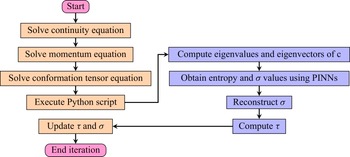
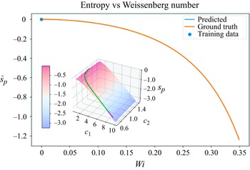


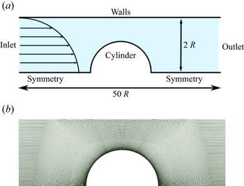
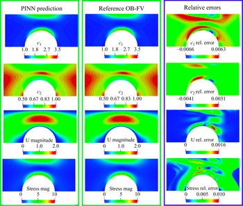

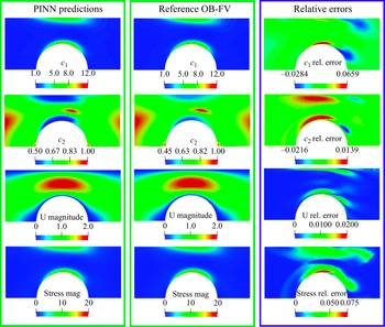


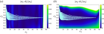


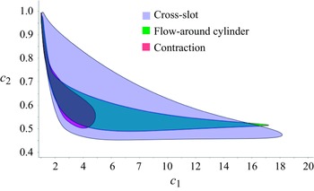


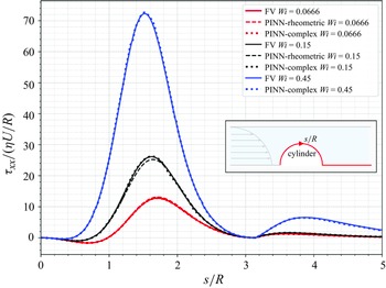

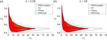


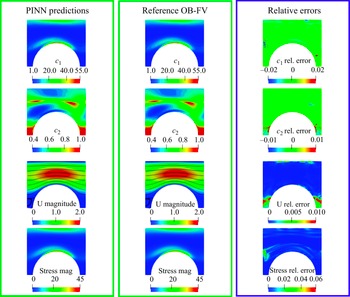


 Open access

