



1. Introduction
Flows at a finite Reynolds number ( $ \textit{Re}$
) have long attracted interest due to their distinctive inertial–viscous coupling characteristics, especially in contexts such as micro-scale biological locomotion and miniature device design (Hopkins & Fauci Reference Hopkins and Fauci2002; Zhou & Fan Reference Zhou and Fan2015; Gibson & Stilwell Reference Gibson and Stilwell2018; Fung, Bearon & Hwang Reference Fung, Bearon and Hwang2022; Wang & Christov Reference Wang and Christov2022). At
$ \textit{Re}$
) have long attracted interest due to their distinctive inertial–viscous coupling characteristics, especially in contexts such as micro-scale biological locomotion and miniature device design (Hopkins & Fauci Reference Hopkins and Fauci2002; Zhou & Fan Reference Zhou and Fan2015; Gibson & Stilwell Reference Gibson and Stilwell2018; Fung, Bearon & Hwang Reference Fung, Bearon and Hwang2022; Wang & Christov Reference Wang and Christov2022). At $ \textit{Re} \leqslant 300$
, the flow resides in a transitional regime: neither dominated purely by viscosity (as in
$ \textit{Re} \leqslant 300$
, the flow resides in a transitional regime: neither dominated purely by viscosity (as in $ \textit{Re} \approx 0$
), nor exhibiting fully developed turbulence (typical of
$ \textit{Re} \approx 0$
), nor exhibiting fully developed turbulence (typical of $ \textit{Re} \gt 10^{4}$
) (Kim & Choi Reference Kim and Choi2002; Li, Xia & Wang Reference Li, Wang, Qiu, Wu, Zhou, Fu and Liu2022a
; Yang, Feng & Zhang Reference Yang, Feng and Zhang2022; Miara et al. Reference Miara, Vaquero-Stainer, Pihler-Puzović, Heil and Juel2024; Nidhan et al. Reference Nidhan, Jain, Ortiz-Tarin and Sarkar2025). Instead, laminar boundary layers coexist with periodic vortex shedding, offering a fundamental platform to explore the synergy between added-mass effects and viscous dissipation (Zhu et al. Reference Zhu, Hu, Zheng and Wang2017; Lagrange & Fraigneau Reference Lagrange and Fraigneau2020; Gupta et al. Reference Gupta, Lo, Zhao, Thompson and Hourigan2025).
$ \textit{Re} \gt 10^{4}$
) (Kim & Choi Reference Kim and Choi2002; Li, Xia & Wang Reference Li, Wang, Qiu, Wu, Zhou, Fu and Liu2022a
; Yang, Feng & Zhang Reference Yang, Feng and Zhang2022; Miara et al. Reference Miara, Vaquero-Stainer, Pihler-Puzović, Heil and Juel2024; Nidhan et al. Reference Nidhan, Jain, Ortiz-Tarin and Sarkar2025). Instead, laminar boundary layers coexist with periodic vortex shedding, offering a fundamental platform to explore the synergy between added-mass effects and viscous dissipation (Zhu et al. Reference Zhu, Hu, Zheng and Wang2017; Lagrange & Fraigneau Reference Lagrange and Fraigneau2020; Gupta et al. Reference Gupta, Lo, Zhao, Thompson and Hourigan2025).
The prolate spheroid has emerged as a canonical model for investigating flow dynamics at finite Reynolds numbers due to its pronounced streamlining characteristics and geometric simplicity (Deng & Caulfield Reference Deng and Caulfield2018; Plasseraud, Kumar & Mahesh Reference Plasseraud, Kumar and Mahesh2023; De Souza et al. Reference De Souza, Ouchene and Thomas2024, Reference De Souza, Ouchene and Thomas2025; Cao et al. Reference Cao, Li, Liu, Zhang, Tafti, Wang, Yuan and Hu2025; Gao et al. Reference Gao, Hu, Meng, Cui, Mao and Liu2025). This canonical model captures key features relevant at both micro and macro scales. For example, it models the behaviour of lignocellulosic fibres in dilute suspensions at small scales, and at larger scales it approximates the hull geometry of underwater vehicles (Jiang et al. Reference Jiang, Andersson, Gallardo and Okulov2016). Accurately predicting unsteady forces and torques on such elongated bodies is crucial for designing attitude control algorithms in micro-electromechanical underwater vehicles (Ayancik et al. Reference Ayancik, Zhong, Quinn, Brandes, Bart-Smith and Moored2019; Kamal & Lauga Reference Kamal and Lauga2023; Anand & Narsimhan Reference Anand and Narsimhan2024). For instance, during trajectory correction phases involving yaw manoeuvres, small-amplitude pitch oscillations frequently occur. In hydrodynamic modelling of underwater vehicles, accurately characterising added-mass and viscous forces is essential for robust control and precise positioning (Will et al. Reference Will, Mathai, Huisman, Lohse, Sun and Krug2021; Jiang et al. Reference Jiang, Wang, Liu, Sun and Calzavarini2022). Moreover, many planktonic organisms (e.g. copepods) rely on pitch oscillations for propulsion and orientation, typically within Reynolds numbers $50 {-} 300$
and pitch amplitudes below
$50 {-} 300$
and pitch amplitudes below $10^{\circ }$
(Guasto et al. Reference Guasto, Johnson and Gollub2010, Reference Guasto, Rusconi and Stocker2012; Eastham & Shoele Reference Eastham and Shoele2020). Understanding the unsteady force dynamics at
$10^{\circ }$
(Guasto et al. Reference Guasto, Johnson and Gollub2010, Reference Guasto, Rusconi and Stocker2012; Eastham & Shoele Reference Eastham and Shoele2020). Understanding the unsteady force dynamics at $ Re \leqslant 300$
in this low-pitch-amplitude regime is thus crucial for decoding the principles of energy-efficient biological locomotion. Such understanding informs the development of biomimetic propulsion systems by elucidating the interplay between vortex-induced pressure gradients and viscous damping in low-inertia flow regimes. This parametric regime effectively bridges the gap between fully viscous-dominated microswimmer dynamics (Li et al. Reference Li, Abbas, Morris, Climent and Magnaudet2020; Ault & Shin Reference Ault and Shin2024; Ishikawa Reference Ishikawa2024) and inertia-dominated macroscopic aquatic locomotion (Huang, Qiu & Wang Reference Huang, Qiu and Wang2022; Li et al. Reference Li, Xia and Wang2022b
, Reference Li, Song, Zhong and Yin2023), offering a foundational framework for optimising energy expenditure in bio-inspired micropropulsors.
$ Re \leqslant 300$
in this low-pitch-amplitude regime is thus crucial for decoding the principles of energy-efficient biological locomotion. Such understanding informs the development of biomimetic propulsion systems by elucidating the interplay between vortex-induced pressure gradients and viscous damping in low-inertia flow regimes. This parametric regime effectively bridges the gap between fully viscous-dominated microswimmer dynamics (Li et al. Reference Li, Abbas, Morris, Climent and Magnaudet2020; Ault & Shin Reference Ault and Shin2024; Ishikawa Reference Ishikawa2024) and inertia-dominated macroscopic aquatic locomotion (Huang, Qiu & Wang Reference Huang, Qiu and Wang2022; Li et al. Reference Li, Xia and Wang2022b
, Reference Li, Song, Zhong and Yin2023), offering a foundational framework for optimising energy expenditure in bio-inspired micropropulsors.
Steady-state correlations for drag, lift and torque coefficients have been extensively studied for prolate spheroids (Jiang et al. Reference Jiang, Andersson, Gallardo and Okulov2016; Sanjeevi et al. Reference Sanjeevi, Kuipers and Padding2018, Reference Sanjeevi, Dietiker and Padding2022; Andersson & Jiang Reference Andersson and Jiang2019; Fröhlich et al. Reference Fröhlich, Meinke and Schröder2020; Fillingham et al. Reference Fillingham, Vaddi, Bruning, Israel and Novosselov2021; Chéron et al. Reference Chéron, Evrard and van Wachem2024; Gorges et al. Reference Gorges, Chéron, Chopra, Denner and van Wachem2025). Their unsteady counterparts, particularly in regimes dominated by added mass effects, remain poorly characterised in terms of both the underlying physics and predictive modelling frameworks. Added mass (or virtual mass) arises from the acceleration of the surrounding fluid along with the body, and plays a pivotal role in the inertial force response during unsteady motion (Korotkin Reference Korotkin2008; Lin & Liao Reference Lin and Liao2011; Ayancik et al. Reference Ayancik, Zhong, Quinn, Brandes, Bart-Smith and Moored2019). Crucially, the added mass influences not only the magnitude of unsteady hydrodynamic forces, but also the phase lag between body motion and fluid loading (Graham, Ford & Babinsky Reference Graham, Ford and Babinsky2017; Limacher Reference Limacher2021; Laín et al. Reference Laín, Castang and Sommerfeld2024, Reference Laín, Castang and Chéron2025). Classical potential flow theory provides analytical solutions for the added mass of idealised bodies such as spheres and ellipsoids. However, as an inviscid framework, it fundamentally neglects viscous effects and consequently fails to capture the viscous–inertial interactions that dominate at finite Reynolds numbers (Li, Xu & Wu Reference Li, Xu and Wu2015; Corkery, Babinsky & Graham Reference Corkery, Babinsky and Graham2019; Essmann et al. Reference Essmann, Shui, Popinet, Zaleski, Valluri and Govindarajan2020; García-Geijo et al. Reference García-Geijo, Riboux and Gordillo2022).
In addition to added mass, unsteady viscous phenomena – particularly flow separation and vortex shedding – represent another source of hydrodynamic forces at finite Reynolds numbers. For prolate spheroids, stable separation vortices emerge along the leeward side when the inclination angle exceeds approximately $40^{\circ }$
, with the shedding frequency often synchronising with the body’s oscillation frequency (Jiang et al. Reference Jiang, Andersson, Gallardo and Okulov2016; Strandenes et al. Reference Strandenes, Jiang, Pettersen and Andersson2019; Guo, Kaiser & Rival Reference Guo, Kaiser and Rival2023b
). Prior studies suggest that limited angular excursions can trigger lock-in phenomena, in which the vortex shedding frequency becomes an integer multiple of the pitching frequency (Kumar, Navrose & Mittal Reference Kumar, Navrose and Mittal2016; Menon & Mittal Reference Menon and Mittal2019; Guo et al. Reference Guo, Kaiser and Rival2023a
). However, such resonance behaviour remains unconfirmed for prolate spheroids pitching at
$40^{\circ }$
, with the shedding frequency often synchronising with the body’s oscillation frequency (Jiang et al. Reference Jiang, Andersson, Gallardo and Okulov2016; Strandenes et al. Reference Strandenes, Jiang, Pettersen and Andersson2019; Guo, Kaiser & Rival Reference Guo, Kaiser and Rival2023b
). Prior studies suggest that limited angular excursions can trigger lock-in phenomena, in which the vortex shedding frequency becomes an integer multiple of the pitching frequency (Kumar, Navrose & Mittal Reference Kumar, Navrose and Mittal2016; Menon & Mittal Reference Menon and Mittal2019; Guo et al. Reference Guo, Kaiser and Rival2023a
). However, such resonance behaviour remains unconfirmed for prolate spheroids pitching at $50 \leqslant Re \leqslant 300$
. From a modelling standpoint, traditional approaches such as the modified Morison equation decompose unsteady loads into inertial (added-mass) and viscous components (Chung Reference Chung2018; Limacher, Morton & Wood Reference Limacher, Morton and Wood2018). Nevertheless, this framework typically assumes a constant force coefficient, thereby failing to capture the nonlinear sensitivity of viscous forces to boundary-layer separation near critical inclination angles (e.g.
$50 \leqslant Re \leqslant 300$
. From a modelling standpoint, traditional approaches such as the modified Morison equation decompose unsteady loads into inertial (added-mass) and viscous components (Chung Reference Chung2018; Limacher, Morton & Wood Reference Limacher, Morton and Wood2018). Nevertheless, this framework typically assumes a constant force coefficient, thereby failing to capture the nonlinear sensitivity of viscous forces to boundary-layer separation near critical inclination angles (e.g. $45^{\circ }$
) (Santo et al. Reference Santo, Taylor, Williamson and Choo2018; Vergara, Wei & Fuentes Reference Vergara, Wei and Fuentes2024).
$45^{\circ }$
) (Santo et al. Reference Santo, Taylor, Williamson and Choo2018; Vergara, Wei & Fuentes Reference Vergara, Wei and Fuentes2024).
In the present study, we investigate the unsteady hydrodynamic response of a prolate spheroid undergoing small-amplitude pitching ( $\pm 5^{\circ }$
) about a baseline inclination
$\pm 5^{\circ }$
) about a baseline inclination $45^{\circ }$
across a range of pitching frequencies. The motion is situated within a separation-prone regime (
$45^{\circ }$
across a range of pitching frequencies. The motion is situated within a separation-prone regime ( $40^{\circ } {-} 50^{\circ }$
) at transitional Reynolds numbers (
$40^{\circ } {-} 50^{\circ }$
) at transitional Reynolds numbers ( $50 {-} 300$
). This configuration is deliberately chosen to probe a near-critical flow state. Under such conditions, the interplay between incipient separation vortices and periodic body motion can lead to complex force and torque dynamics. Despite its practical relevance in both biological and engineering systems, this near-separation state remains poorly characterised in terms of both force generation mechanisms and modelling frameworks. To address this gap, we conduct high-resolution numerical simulations to resolve the unsteady flow structures and quantify the associated hydrodynamic loads. Particular attention is given to disentangling the contributions of added mass and viscous effects, and to identifying the nonlinear interactions that arise due to flow–body coupling. The research outcomes are expected to establish quantitative correlations for unsteady force and torque characteristics of pitching prolate spheroids, explicitly incorporating both added-mass contributions and viscous effects.
$50 {-} 300$
). This configuration is deliberately chosen to probe a near-critical flow state. Under such conditions, the interplay between incipient separation vortices and periodic body motion can lead to complex force and torque dynamics. Despite its practical relevance in both biological and engineering systems, this near-separation state remains poorly characterised in terms of both force generation mechanisms and modelling frameworks. To address this gap, we conduct high-resolution numerical simulations to resolve the unsteady flow structures and quantify the associated hydrodynamic loads. Particular attention is given to disentangling the contributions of added mass and viscous effects, and to identifying the nonlinear interactions that arise due to flow–body coupling. The research outcomes are expected to establish quantitative correlations for unsteady force and torque characteristics of pitching prolate spheroids, explicitly incorporating both added-mass contributions and viscous effects.
A well-established modelling approach for offshore structures decomposes unsteady hydrodynamic loads into drag (quasi-steady) and inertial (acceleration-dependent) components. This framework originated with Morison, Johnson & Schaaf (Reference Morison, Johnson and Schaaf1950), who developed an empirical force model for waves acting on vertical cylindrical piles, validated experimentally. Their formulation – the Morison equation – became a cornerstone of offshore hydrodynamics. Sarpkaya (Reference Sarpkaya2010) later analysed wave–structure interactions, highlighting limitations of the classical decomposition under separated flows and vortex shedding. His work clarified the interplay between inertial, drag and lift forces in oscillatory conditions, particularly during vortex-induced vibrations. This work revealed the need for models beyond the empirical Morison equation. More recently, Wood & Oudah (Reference Wood and Oudah2025) tackled another limitation: the assumption of rigid pile response. They introduced a modified Morison equation, scaling total wave force by a dynamic amplification factor. Calibrated through extensive simulations, this factor incorporates pile flexibility, boundary conditions and wave properties, improving force predictions for flexible piled wharves. Based on this evolving foundation, the current study extends the framework to pitching prolate spheroids at transitional Reynolds numbers. The inertial (added-mass) term is decomposed into a potential-flow fundamental solution and a viscous correction. A unified hybrid correlation, valid across the studied frequency and Reynolds number ranges, is proposed. Physically, the viscous correction represents damping linked to hairpin vortex structures and flow separation. While the overall force decomposition follows the classical Morison form, the present extensions enable the capture of frequency-dependent phase shifts and asymmetries in the unsteady forces.
The remainder of this paper is structured as follows. In § 2, we introduce the numerical model and methods for the flow around a prolate spheroid, detailing and validating the computational framework. In § 3, we analyse the time-averaged and phase-resolved behaviour of drag, lift and torque coefficients across various pitching frequencies, with particular emphasis on quantifying unsteady effects through comparison with quasi-steady theoretical predictions. In § 4, we provide mathematical expressions for added-mass forces and torques acting on pitching prolate spheroids under potential flow assumptions. Building upon these foundations, we propose and validate a novel hybrid correlation that concurrently accounts for both added-mass and viscous effects. Finally, § 5 synthesises key findings and discusses their implications for modelling of pitching prolate spheroids.
2. Numerical model and method
2.1. Problem set-ups
We investigate the flow around a prolate spheroid pitching in a uniform upstream flow $U_{\infty }$
. Figure 1(a) sketches the geometric model of the prolate spheroid and its associated Cartesian coordinate systems. The earth-fixed system (
$U_{\infty }$
. Figure 1(a) sketches the geometric model of the prolate spheroid and its associated Cartesian coordinate systems. The earth-fixed system ( $X$
,
$X$
, $Y$
,
$Y$
, $Z$
) has its
$Z$
) has its $X$
-axis aligned with the streamwise direction. The body-fixed system (
$X$
-axis aligned with the streamwise direction. The body-fixed system ( $\hat {X}$
,
$\hat {X}$
, $\hat {Y}$
,
$\hat {Y}$
, $\hat {Z}$
) is defined with the
$\hat {Z}$
) is defined with the $\hat {X}$
-axis along the prolate spheroid’s major axis. The prolate spheroid pitches around the
$\hat {X}$
-axis along the prolate spheroid’s major axis. The prolate spheroid pitches around the $\hat {Z}$
-axis, which is located at the centre of the prolate spheroid. The origin and
$\hat {Z}$
-axis, which is located at the centre of the prolate spheroid. The origin and $Z$
-axis of both coordinate systems coincide at the initial moment. In the body-fixed coordinate system, the coordinates (
$Z$
-axis of both coordinate systems coincide at the initial moment. In the body-fixed coordinate system, the coordinates ( $\hat {x}$
,
$\hat {x}$
, $\hat {y}$
,
$\hat {y}$
, $\hat {z}$
) of the surface of the prolate spheroid (Miao & Xiao Reference Miao and Xiao2021; Hu et al. Reference Hu, Lin, Zhu, Yu, Lin and Li2024) are consistent with
$\hat {z}$
) of the surface of the prolate spheroid (Miao & Xiao Reference Miao and Xiao2021; Hu et al. Reference Hu, Lin, Zhu, Yu, Lin and Li2024) are consistent with
 \begin{align} \frac {\hat {x}^{2} }{a^{2}} +\frac {\hat {y}^{2} }{b^{2}}+\frac {\hat {z}^{2} }{c^{2}}=1, \end{align}
where $a$
is the semi-major axis, and
$a$
is the semi-major axis, and $b=c$
is the semi-minor axis. Here, the prolate spheroid’s minor-axis diameter is
$b=c$
is the semi-minor axis. Here, the prolate spheroid’s minor-axis diameter is $D=2b$
, and its aspect ratio is defined as
$D=2b$
, and its aspect ratio is defined as $\beta = a/b$
.
$\beta = a/b$
.
Schematic of the computational set-up for the problem: (a) the two Cartesian coordinate systems; (b) the flow configuration in a three-dimensional rectangular box.

Figure 1. Long description
Panel A: A diagram showing two Cartesian coordinate systems. The first coordinate system is labeled with axes X, Y, and Z, and the second coordinate system is labeled with axes X-hat, Y-hat, and Z-hat. The prolate spheroid is positioned at the origin of both coordinate systems, with its major axis aligned along the X-axis. The angle phi represents the pitch angle between the two coordinate systems. The dimensions of the prolate spheroid are given as a equals 3D and b equals 0.5D, where D is a characteristic length. The free stream velocity U-infinity is directed along the X-axis. Panel B: A three-dimensional rectangular box representing the flow configuration. The box has dimensions 24D by 11D by 40D. The prolate spheroid is placed within the box, and its position and orientation are defined by the overset region. The flow enters the box at the inlet and exits at the outlet. The wake region downstream of the prolate spheroid is also depicted. The axes X, Y, and Z are labeled, and the pitch angle is indicated.
The kinematics of the prolate spheroid are prescribed by changing the inclination angle
 \begin{align} \phi \left ( t \right ) =\phi _{0} +\phi _{m}\sin \left ( 2\pi f t \right ), \end{align}
where $\phi _{0}$
is the average intersection angle of the
$\phi _{0}$
is the average intersection angle of the $X$
-axis and
$X$
-axis and $\hat {X}$
-axis, and
$\hat {X}$
-axis, and $\phi _{m}$
is the pitching amplitude. The non-dimensional pitching frequency is given by
$\phi _{m}$
is the pitching amplitude. The non-dimensional pitching frequency is given by $f=f_{*}D/U_{\infty }$
, where
$f=f_{*}D/U_{\infty }$
, where $f_{*}$
denotes the dimensional pitching frequency. Similarly, non-dimensional time is defined as
$f_{*}$
denotes the dimensional pitching frequency. Similarly, non-dimensional time is defined as $t=t_{*}U_{\infty }/D$
, with
$t=t_{*}U_{\infty }/D$
, with $t_{*}$
representing dimensional time. A complete non-dimensional pitching period is given by
$t_{*}$
representing dimensional time. A complete non-dimensional pitching period is given by $T=1/f$
.
$T=1/f$
.
2.2. Numerical method
The unsteady flow around the pitching prolate spheroid is governed by the Navier–Stokes equations for incompressible flows:
 \begin{align} \frac {\partial \boldsymbol{u}}{\partial t}+\boldsymbol{u}\boldsymbol{\cdot } \boldsymbol{\nabla }\boldsymbol{u} & = - \boldsymbol{\nabla }p+\frac {1}{Re_{D}} \nabla ^{2} \boldsymbol{u}, \\[-12pt] \nonumber \end{align}
 \begin{align} \boldsymbol{\nabla } \boldsymbol{\cdot }\boldsymbol{u} & = 0, \\[10pt] \nonumber \end{align}
where $\boldsymbol{u} = ( u_{x} ,u_{y} ,u_{z})$
denotes the velocity vector in the Cartesian coordinates,
$\boldsymbol{u} = ( u_{x} ,u_{y} ,u_{z})$
denotes the velocity vector in the Cartesian coordinates, $p$
denotes the pressure, and
$p$
denotes the pressure, and $ \textit{Re}_{D}=U_{\infty }D/\nu$
denotes the Reynolds number, with
$ \textit{Re}_{D}=U_{\infty }D/\nu$
denotes the Reynolds number, with $\nu$
the kinematic viscosity. The uniform free-stream velocity (
$\nu$
the kinematic viscosity. The uniform free-stream velocity ( $U_{\infty }$
) is arranged at the inlet, and the fixed pressure condition is stipulated at the outlet. The slip-wall condition is operated at the other boundaries, and the no-slip condition is stated on the prolate spheroid.
$U_{\infty }$
) is arranged at the inlet, and the fixed pressure condition is stipulated at the outlet. The slip-wall condition is operated at the other boundaries, and the no-slip condition is stated on the prolate spheroid.
The governing equations are discretised on an unstructured mesh using the finite volume method (Manik, Dalal & Natarajan Reference Manik, Dalal and Natarajan2018). The time derivative is discretised with a second-order implicit backward scheme with an adaptive time-stepping protocol employing a dynamic global Courant number constraint ( $\text{CFL} \leqslant 0.8$
). Spatial discretisation adopts the second-order central differencing scheme. For solving the discretised equations, the preconditioned bi-conjugate gradient method with a diagonal-based incomplete LU preconditioner is used for the pressure fields. The reader can refer to Mokalled, Mangani & Darwish (Reference Mokalled, Mangani and Darwish2016) for more detailed descriptions of the numerical implementation.
$\text{CFL} \leqslant 0.8$
). Spatial discretisation adopts the second-order central differencing scheme. For solving the discretised equations, the preconditioned bi-conjugate gradient method with a diagonal-based incomplete LU preconditioner is used for the pressure fields. The reader can refer to Mokalled, Mangani & Darwish (Reference Mokalled, Mangani and Darwish2016) for more detailed descriptions of the numerical implementation.
The three-dimensional view of the pitching prolate spheroid is shown in figure 1(b). The present simulation is performed in a rectangular domain $[ -8 D, 32 D ] \times [ -8 D, 16 D ] \times [ -5.5 D, 5.5 D ]$
. This study concerns a prolate spheroid with a constant aspect ratio
$[ -8 D, 32 D ] \times [ -8 D, 16 D ] \times [ -5.5 D, 5.5 D ]$
. This study concerns a prolate spheroid with a constant aspect ratio $\beta = 6$
and baseline inclination
$\beta = 6$
and baseline inclination $\phi _{0} = 45^{\circ }$
. Consequently, the computational domain dimensions are identical for all cases; their verification is provided in Appendix A. In this study, we consider a range of Reynolds numbers (
$\phi _{0} = 45^{\circ }$
. Consequently, the computational domain dimensions are identical for all cases; their verification is provided in Appendix A. In this study, we consider a range of Reynolds numbers ( $ \textit{Re}_{D}$
)
$ \textit{Re}_{D}$
) $50{-}300$
. Notably, the diameter of the volume-equivalent sphere (
$50{-}300$
. Notably, the diameter of the volume-equivalent sphere ( $d =2 \sqrt [3]{ab^{2} }=\sqrt [3]{\beta }\, D$
) is used as the characteristic length to calculate the Reynolds number in some of the literature (Zhang, Ni & Magnaudet Reference Zhang, Ni and Magnaudet2021; Sanjeevi, Dietiker & Padding Reference Sanjeevi, Dietiker and Padding2022; Wang et al. Reference Wang, Yang, Andersson, Zhu, Wu, Wang and Liu2022; Shi, Zhang & Magnaudet Reference Shi, Zhang and Magnaudet2024), i.e.
$d =2 \sqrt [3]{ab^{2} }=\sqrt [3]{\beta }\, D$
) is used as the characteristic length to calculate the Reynolds number in some of the literature (Zhang, Ni & Magnaudet Reference Zhang, Ni and Magnaudet2021; Sanjeevi, Dietiker & Padding Reference Sanjeevi, Dietiker and Padding2022; Wang et al. Reference Wang, Yang, Andersson, Zhu, Wu, Wang and Liu2022; Shi, Zhang & Magnaudet Reference Shi, Zhang and Magnaudet2024), i.e. $ \textit{Re}_{d} = U_{\infty } d / \nu$
. We perform a series of numerical simulations using the OpenFOAM package, with the parameters varied as listed in table 1. The effects of different pitching frequencies on the hydrodynamic and flow-field characteristics of the prolate spheroid are considered. The
$ \textit{Re}_{d} = U_{\infty } d / \nu$
. We perform a series of numerical simulations using the OpenFOAM package, with the parameters varied as listed in table 1. The effects of different pitching frequencies on the hydrodynamic and flow-field characteristics of the prolate spheroid are considered. The $45^{\circ }$
initial inclination angle selected in this study serves as a typical threshold for boundary-layer separation in bluff body flows (Lim, Castro & Hoxey Reference Lim, Castro and Hoxey2007; Kumar et al. Reference Kumar, Sourav, Sen and Yadav2018; Zigunov, Sellappan & Alvi Reference Zigunov, Sellappan and Alvi2020). It represents a critical condition where small changes in vortex dynamics strongly influence unsteady loads. This configuration provides an opportunity to probe the nonlinear interplay between added-mass forces and viscous separation, making it an ideal test case for assessing hybrid models. In the low-frequency regime, the combination of a
$45^{\circ }$
initial inclination angle selected in this study serves as a typical threshold for boundary-layer separation in bluff body flows (Lim, Castro & Hoxey Reference Lim, Castro and Hoxey2007; Kumar et al. Reference Kumar, Sourav, Sen and Yadav2018; Zigunov, Sellappan & Alvi Reference Zigunov, Sellappan and Alvi2020). It represents a critical condition where small changes in vortex dynamics strongly influence unsteady loads. This configuration provides an opportunity to probe the nonlinear interplay between added-mass forces and viscous separation, making it an ideal test case for assessing hybrid models. In the low-frequency regime, the combination of a $5^{\circ }$
pitching amplitude and a non-dimensional pitching frequency (
$5^{\circ }$
pitching amplitude and a non-dimensional pitching frequency ( $f=0{-} 0.16$
) can simulate either the attitude fine-tuning of underwater vehicles or the pulsed pitching kinematics witnessed in biological propulsion systems.
$f=0{-} 0.16$
) can simulate either the attitude fine-tuning of underwater vehicles or the pulsed pitching kinematics witnessed in biological propulsion systems.
List of cases investigated in this study.

Table 1. Long description
TA table with three columns and nine rows. The columns are labeled ‘Cases’, ‘Re_D’, and ‘f’. The ‘Cases’ column lists specific case numbers or ranges. The ‘Re_D’ column lists Reynolds numbers: 200 for case 1 and 50, 100, 150, 200, 250, 300 for cases 2-43. The ‘f’ column lists frequencies: 0 for case 1 and 0.032, 0.040, 0.053, 0.080, 0.106, 0.128, 0.160 for cases 2-43. The table organizes cases by ranges and provides corresponding Reynolds numbers and frequencies for each case.
The unstructured overset mesh: three levels of local Cartesian mesh refinement, and a detailed view of the near-wall boundary layer and overset mesh.

An overset mesh approach (Brazell, Sitaraman & Mavriplis Reference Brazell, Sitaraman and Mavriplis2016; Morse & Mahesh Reference Morse and Mahesh2021; Lin et al. Reference Lin, Zhu, Liu and Wang2026) is used to handle the prolate spheroid’s pitching motion. The unstructured overset mesh with local mesh refinement is shown in figure 2. The size of the grid is multiplicatively related to the refinement levels of the grid. A locally refined mesh is employed, with minimum spacing ( $0.05D$
in all three directions) near the body surface (level 3), specifically within the prismatic mesh layers (Roget et al. Reference Roget, Sitaraman, Lakshminarayan and Wissink2020; Ye et al. Reference Ye, Liu, Ni and Chen2025). The dimensionless wall distance
$0.05D$
in all three directions) near the body surface (level 3), specifically within the prismatic mesh layers (Roget et al. Reference Roget, Sitaraman, Lakshminarayan and Wissink2020; Ye et al. Reference Ye, Liu, Ni and Chen2025). The dimensionless wall distance $y^{+} \lt 1$
ensures resolution of the viscous sublayer. Coarser spacing (
$y^{+} \lt 1$
ensures resolution of the viscous sublayer. Coarser spacing ( $0.4D$
in all three directions) is used in the far field (level 0) to reduce computational cost. The overset grid and the nearby background grid have the same mesh density (level 3) to facilitate data exchange at the overset boundaries. The total number of cells is approximately 17 million. By altering the size of the grid, a convergence test has confirmed the validity of the current set-up, as detailed in Appendix A.
$0.4D$
in all three directions) is used in the far field (level 0) to reduce computational cost. The overset grid and the nearby background grid have the same mesh density (level 3) to facilitate data exchange at the overset boundaries. The total number of cells is approximately 17 million. By altering the size of the grid, a convergence test has confirmed the validity of the current set-up, as detailed in Appendix A.
2.3. Force and torque coefficients
The drag force ( $F_{x}$
) acting upon a prolate spheroid is aligned with the direction of the flow and is characterised by the drag coefficient (
$F_{x}$
) acting upon a prolate spheroid is aligned with the direction of the flow and is characterised by the drag coefficient ( $C_{\kern-1pt D}$
), which is defined as
$C_{\kern-1pt D}$
), which is defined as
 \begin{align} C_{\kern-1pt D} =\frac {F_{x}}{\frac {1}{2} \rho U_{\infty }^{2} \frac {\pi }{4} d^{2} } , \end{align}
where $\rho$
denotes the fluid density. Here, defining the reference area as the cross-sectional area of a volume-equivalent sphere ensures that it remains constant irrespective of the angle of incidence.
$\rho$
denotes the fluid density. Here, defining the reference area as the cross-sectional area of a volume-equivalent sphere ensures that it remains constant irrespective of the angle of incidence.
The lift force ( $F_{y}$
) acts in a direction perpendicular to the upstream flow velocity and can be characterised by a lift coefficient (
$F_{y}$
) acts in a direction perpendicular to the upstream flow velocity and can be characterised by a lift coefficient ( $C_{L}$
), which is defined as
$C_{L}$
), which is defined as
 \begin{align} C_{L} =\frac {F_{y}}{\frac {1}{2} \rho U_{\infty }^{2} \frac {\pi }{4} d^{2} }. \end{align}
The pitching torque around the $Z$
-axis (
$Z$
-axis ( $M_{z}$
) can be characterised by the torque coefficient (
$M_{z}$
) can be characterised by the torque coefficient ( $C_{T}$
), which is defined as
$C_{T}$
), which is defined as
 \begin{align} C_{T} =\frac {M_{z}}{\frac {1}{2} \rho U_{\infty }^{2} \frac {\pi }{8} d^{3} }. \end{align}
The time-averaged force and torque coefficients are defined as
 \begin{align} \bar {C}_{D} = \frac {1}{\frac {1}{2} \rho U_{\infty }^{2} \frac {\pi }{4} d^{2} } \times\frac {1}{\textit{NT}} \int _{t_{0} }^{t_{0}+\textit{NT}} F_{x} (t) \,\mathrm{d}t, \\[-12pt] \nonumber \end{align}
 \begin{align} \bar {C}_{L} = \frac {1}{\frac {1}{2} \rho U_{\infty }^{2} \frac {\pi }{4} d^{2} } \times\frac {1}{\textit{NT}} \int _{t_{0} }^{t_{0}+\textit{NT}} F_{y} (t) \,\mathrm{d}t, \\[-12pt] \nonumber \end{align}
 \begin{align} \bar {C}_{T} = \frac {1}{\frac {1}{2} \rho U_{\infty }^{2} \frac {\pi }{8} d^{3} } \times\frac {1}{\textit{NT}} \int _{t_{0} }^{t_{0}+\textit{NT}} M_{z}(t) \,\mathrm{d}t, \\[10pt] \nonumber \end{align}
where $t_0$
denotes the starting instant for averaging, commencing once the flow has attained a statistically periodic state, and
$t_0$
denotes the starting instant for averaging, commencing once the flow has attained a statistically periodic state, and $N$
represents the number of pitching periods over which the averaging is performed. In this study, value
$N$
represents the number of pitching periods over which the averaging is performed. In this study, value $N = 5$
is adopted.
$N = 5$
is adopted.
3. Results and discussion
3.1. Time-averaged force coefficients and flow fields
Comparative analysis of simulation data and correlation results of time-averaged (a) drag, (b) lift and (c) torque coefficients versus various Reynolds numbers for the prolate spheroid at different pitching frequencies.

Figure 3. Long description
Three line graphs depict the comparative analysis of simulation data and correlation results of time-averaged coefficients versus Reynolds numbers for a prolate spheroid at different pitching frequencies. Panel A: The line graph shows the drag coefficient (C D) on the vertical axis and Reynolds number (Re D) on the horizontal axis. Multiple lines represent different pitching frequencies, with markers indicating simulation data points and lines representing correlation results. The drag coefficient decreases as the Reynolds number increases. Panel B: The line graph shows the lift coefficient (C L) on the vertical axis and Reynolds number (Re D) on the horizontal axis. Similar to Panel A, multiple lines represent different pitching frequencies, with markers for simulation data and lines for correlation results. The lift coefficient slightly decreases and then stabilizes as the Reynolds number increases. Panel C: The line graph shows the torque coefficient (C T) on the vertical axis and Reynolds number (Re D) on the horizontal axis. Multiple lines represent different pitching frequencies, with markers for simulation data and lines for correlation results. The torque coefficient decreases as the Reynolds number increases.
In this subsection, we report the time-averaged drag ( $\bar {C}_{D}$
), lift (
$\bar {C}_{D}$
), lift ( $\bar {C}_{L}$
) and torque (
$\bar {C}_{L}$
) and torque ( $\bar {C}_{T}$
) coefficients obtained from numerical simulations of flows around prolate spheroids at different dimensionless pitching frequencies (
$\bar {C}_{T}$
) coefficients obtained from numerical simulations of flows around prolate spheroids at different dimensionless pitching frequencies ( $f$
) and Reynolds numbers (
$f$
) and Reynolds numbers ( $ \textit{Re}_{D}$
). Figure 3 indicates significant Reynolds number dependence, with variations of up to 44.01 % in drag, 8.31 % in lift, and 15.38 % in torque between
$ \textit{Re}_{D}$
). Figure 3 indicates significant Reynolds number dependence, with variations of up to 44.01 % in drag, 8.31 % in lift, and 15.38 % in torque between $ \textit{Re}_{D}=50$
and
$ \textit{Re}_{D}=50$
and $ \textit{Re}_{D}=300$
at identical pitching frequencies. The drag coefficient emerges as most susceptible to Reynolds number variations. Notably, while all hydrodynamic coefficients display generally diminishing magnitudes with increasing Reynolds numbers, the lift coefficient shows little difference when
$ \textit{Re}_{D}=300$
at identical pitching frequencies. The drag coefficient emerges as most susceptible to Reynolds number variations. Notably, while all hydrodynamic coefficients display generally diminishing magnitudes with increasing Reynolds numbers, the lift coefficient shows little difference when $100 \leqslant Re_{D} \leqslant 300$
. In contrast, the dimensionless pitching frequency of the prolate spheroid exhibits a comparatively minor influence on the time-averaged hydrodynamic coefficients across the Reynolds numbers considered. As illustrated in figure 4, the peak variations between
$100 \leqslant Re_{D} \leqslant 300$
. In contrast, the dimensionless pitching frequency of the prolate spheroid exhibits a comparatively minor influence on the time-averaged hydrodynamic coefficients across the Reynolds numbers considered. As illustrated in figure 4, the peak variations between $ \textit{Re}_{D}=50$
and
$ \textit{Re}_{D}=50$
and $ \textit{Re}_{D}=300$
reach only 2.90 % (drag), 3.11 % (lift) and 2.68 % (torque). The investigation reveals obvious monotonic trends in the frequency-dependent evolution of time-averaged force and torque coefficients across the studied regime. At low frequencies (
$ \textit{Re}_{D}=300$
reach only 2.90 % (drag), 3.11 % (lift) and 2.68 % (torque). The investigation reveals obvious monotonic trends in the frequency-dependent evolution of time-averaged force and torque coefficients across the studied regime. At low frequencies ( $f \leqslant 0.053$
), all hydrodynamic coefficients tend towards constant values, which is consistent with the quasi-steady flow assumptions. As frequency increases, the coefficients deviate from quasi-steady predictions, indicating nonlinear vortex interactions. The drag coefficient shows near-linear augmentation, attaining an elevation at
$f \leqslant 0.053$
), all hydrodynamic coefficients tend towards constant values, which is consistent with the quasi-steady flow assumptions. As frequency increases, the coefficients deviate from quasi-steady predictions, indicating nonlinear vortex interactions. The drag coefficient shows near-linear augmentation, attaining an elevation at $f=0.160$
. This phenomenon occurs as the high-frequency pitching motion leads to rapid changes in surface velocity, thereby augmenting both shear stress and form drag (Alam & Muhammad Reference Alam and Muhammad2020; Sanmiguel-Rojas, Perona & Fernandez-Feria Reference Sanmiguel-Rojas, Perona and Fernandez-Feria2023).
$f=0.160$
. This phenomenon occurs as the high-frequency pitching motion leads to rapid changes in surface velocity, thereby augmenting both shear stress and form drag (Alam & Muhammad Reference Alam and Muhammad2020; Sanmiguel-Rojas, Perona & Fernandez-Feria Reference Sanmiguel-Rojas, Perona and Fernandez-Feria2023).
Based on the characteristics of the simulation results, regression analyses are performed with the nonlinear power function for these hydrodynamic coefficients. To quantitatively describe the hydrodynamic characteristics of the prolate spheroid at different pitching frequencies and Reynolds numbers, correlations for the time-averaged force and torque coefficients are established. The correlations are well fitted to the simulation data points, with a maximum relative error less than 2 %, as shown in figures 3 and 4. These correlations are given by
 \begin{align} \bar {C}_{D}\left ( \breve {f} , \breve {Re_{D}} \right ) = \backepsilon _{11} + \backepsilon _{12} \breve {f} ^{\backepsilon _{13}} + \backepsilon _{14} \breve {Re_{D}} ^{\backepsilon _{15}} + \backepsilon _{16} \breve {f} ^{\backepsilon _{13}} \breve {Re_{D}} ^{\backepsilon _{15}} , \\[-12pt] \nonumber \end{align}
 \begin{align} \bar {C}_{L}\left ( \breve {f} , \breve {Re_{D}} \right ) = \backepsilon _{21} + \backepsilon _{22} \breve {f} ^{\backepsilon _{23}} + \backepsilon _{24} \breve {Re_{D}} ^{\backepsilon _{25}} + \backepsilon _{26} \breve {f} ^{\backepsilon _{23}} \breve {Re_{D}} ^{\backepsilon _{25}} , \\[-12pt] \nonumber \end{align}
 \begin{align} \bar {C}_{T}\left ( \breve {f} , \breve {Re_{D}} \right ) =\backepsilon _{31} + \backepsilon _{32} \breve {f} ^{\backepsilon _{33}} + \backepsilon _{34} \breve {Re_{D}} ^{\backepsilon _{35}} + \backepsilon _{36} \breve {f} ^{\backepsilon _{33}} \breve {Re_{D}} ^{\backepsilon _{35}}, \\[10pt] \nonumber \end{align}
where $\backepsilon _{\textit{ij}}$
(
$\backepsilon _{\textit{ij}}$
( $i=1,2,3$
and
$i=1,2,3$
and $j=1{\sim}6$
) denotes the fitting coefficients for the correlations of time-averaged hydrodynamic coefficients, as provided in table 2. The terms
$j=1{\sim}6$
) denotes the fitting coefficients for the correlations of time-averaged hydrodynamic coefficients, as provided in table 2. The terms $\breve {f}$
and
$\breve {f}$
and $\breve {Re_{D}}$
map the frequency and Reynolds number ranges onto the interval
$\breve {Re_{D}}$
map the frequency and Reynolds number ranges onto the interval $[0, 1]$
, ensuring that the fitting coefficients remain of comparable orders of magnitude, and enhancing the numerical stability of the regression.
$[0, 1]$
, ensuring that the fitting coefficients remain of comparable orders of magnitude, and enhancing the numerical stability of the regression.
Comparative analysis of simulation data and correlation results of time-averaged (a) drag, (b) lift and (c) torque coefficients versus various pitching frequencies for the prolate spheroid at different Reynolds numbers.

The variations of the hydrodynamic coefficients shown in figure 4 can be interpreted by examining the evolution of the vortex system around the pitching spheroid (figure 5). At low frequencies ( $f\lt 0.053$
), the wake is dominated by two symmetric vortex tube patterns, resembling the quasi-steady pattern observed for the fixed-inclination case (
$f\lt 0.053$
), the wake is dominated by two symmetric vortex tube patterns, resembling the quasi-steady pattern observed for the fixed-inclination case ( $\phi =45^{\circ }$
) in Appendix A. However, the pitching motion introduces additional unsteadiness, leading to the periodic formation of hairpin vortices that shed downstream in a highly organised manner. This controlled shedding process enables the development of a compact vortex chain.
$\phi =45^{\circ }$
) in Appendix A. However, the pitching motion introduces additional unsteadiness, leading to the periodic formation of hairpin vortices that shed downstream in a highly organised manner. This controlled shedding process enables the development of a compact vortex chain.
Summary of fitting coefficients of the correlations for time-averaged force coefficients.

Table 2. Long description
TA table summarizing fitting coefficients of correlations for time-averaged force coefficients. The table has 3 rows and 6 columns. The columns are labeled as j = 1, j = 2, j = 3, j = 4, j = 5, and j = 6. The rows are labeled as backepsilon 1j, backepsilon 2j, and backepsilon 3j. Row 1: backepsilon 1j, 1.705, 0.013, 1.251, -0.770, 0.334, 0.018. Row 2: backepsilon 2j, 0.699, 0.014, 1.303, -0.056, 0.016, 0.005. Row 3: backepsilon 3j, 1.068, -0.010, 1.452, -0.151, 0.285, -0.014.
As the pitching frequency increases, the flow topology changes substantially. The accelerated motion disrupts the boundary-layer development and triggers earlier separation of the primary shear layer (see figure 6), which results in premature vortex formation and enhanced pressure drag. Simultaneously, the hairpin structures become more closely spaced and exhibit larger, tilted heads, features that are directly associated with the observed increase in lift coefficient. The increased encounter rate between the spheroid and undisturbed fluid parcels at higher frequencies further enhances the pressure differential between the upper and lower surfaces, thereby amplifying lift generation. Regarding torque coefficient, sufficient spheroid–fluid interaction at lower frequencies generates greater torque magnitude. The torque diminishes with increasing frequency values as reduced temporal allowance prevents equivalent interaction levels between the spherical surface and surrounding fluid medium.
Iso-surfaces of the $Q$
-function at various pitching frequencies, coloured by dimensionless streamwise vorticity (
$Q$
-function at various pitching frequencies, coloured by dimensionless streamwise vorticity ( $\varpi _{x} D/U_{\infty }$
) when
$\varpi _{x} D/U_{\infty }$
) when $ \textit{Re}_{D}=200$
, with two orthogonal views: the first column shows front views, and the second column shows upward views.
$ \textit{Re}_{D}=200$
, with two orthogonal views: the first column shows front views, and the second column shows upward views.

The flow visualisations in figure 6 provide additional physical insight into these trends. The flow fields indicate a marked transition in vortex and pressure distribution as the pitching frequency increases. At the lower frequency ( $f=0.032$
), the flow remains quasi-steady, with weakly developed vorticity concentrated near the trailing edge; correspondingly, the pressure coefficient contours exhibit smooth gradients and sustained suction over the lower surface, indicative of stable lift generation. In contrast, the higher-frequency case (
$f=0.032$
), the flow remains quasi-steady, with weakly developed vorticity concentrated near the trailing edge; correspondingly, the pressure coefficient contours exhibit smooth gradients and sustained suction over the lower surface, indicative of stable lift generation. In contrast, the higher-frequency case ( $f=0.160$
) elicits a pronounced unsteady effect: tightly packed, alternating vortices are shed in the wake, accompanied by intensified local vorticity and highly oscillatory pressure distributions – particularly evident in the sharp suction peaks near the trailing edge. These features reflect an enhanced unsteady shedding regime, wherein the positive pressure region behind the trailing edge generates a pronounced adverse pressure gradient, causing the flow to separate earlier, and amplifying hydrodynamic load fluctuations, thereby intensifying the unsteady forces acting upon the prolate spheroid. The cyclic shedding of this vortex explains both the enhanced lift response and the increased normalised root mean square error (NRMSE) of the lift coefficient at high frequencies (see § 4.2).
$f=0.160$
) elicits a pronounced unsteady effect: tightly packed, alternating vortices are shed in the wake, accompanied by intensified local vorticity and highly oscillatory pressure distributions – particularly evident in the sharp suction peaks near the trailing edge. These features reflect an enhanced unsteady shedding regime, wherein the positive pressure region behind the trailing edge generates a pronounced adverse pressure gradient, causing the flow to separate earlier, and amplifying hydrodynamic load fluctuations, thereby intensifying the unsteady forces acting upon the prolate spheroid. The cyclic shedding of this vortex explains both the enhanced lift response and the increased normalised root mean square error (NRMSE) of the lift coefficient at high frequencies (see § 4.2).
Flow fields at two representative pitching frequencies ( $f=0.032$
and
$f=0.032$
and $f=0.160$
) for
$f=0.160$
) for $ \textit{Re}_{D}=200$
: (a,b) streamlines coloured by dimensionless transverse vorticity (
$ \textit{Re}_{D}=200$
: (a,b) streamlines coloured by dimensionless transverse vorticity ( $\varpi _{z} D/U_{\infty }$
); (c,d) corresponding pressure coefficient (
$\varpi _{z} D/U_{\infty }$
); (c,d) corresponding pressure coefficient ( $C_{p}=p /( 0.5\rho U_{\infty }^{2} )$
) contours.
$C_{p}=p /( 0.5\rho U_{\infty }^{2} )$
) contours.

Figure 6. Long description
Panel A: A streamline plot colored by dimensionless transverse vorticity for a pitching frequency of 0.032. The horizontal axis is labeled X over D, and the vertical axis is labeled Y over D. The color scale ranges from -2 to 2. Panel B: A streamline plot colored by dimensionless transverse vorticity for a pitching frequency of 0.160. The horizontal axis is labeled X over D, and the vertical axis is labeled Y over D. The color scale ranges from -2 to 2. Panel C: A contour plot of the pressure coefficient for a pitching frequency of 0.032. The horizontal axis is labeled X over D, and the vertical axis is labeled Y over D. The color scale ranges from -0.4 to 0.4. Panel D: A contour plot of the pressure coefficient for a pitching frequency of 0.160. The horizontal axis is labeled X over D, and the vertical axis is labeled Y over D. The color scale ranges from -0.4 to 0.4.
3.2. Unsteady wake
The unsteady wake response offers insight into the physical mechanisms underlying the force acting upon a pitching prolate spheroid. Figure 7 presents the temporal evolution of the inclination angle and wake structures for the representative case $f=0.080$
. Three characteristic time instants within a pitching period (
$f=0.080$
. Three characteristic time instants within a pitching period ( $t/T=0.25$
, 0.5 and 0.75) are selected to illustrate the evolution of vortical structures and their interaction with the surrounding flow.
$t/T=0.25$
, 0.5 and 0.75) are selected to illustrate the evolution of vortical structures and their interaction with the surrounding flow.
(a) Evolution curves of inclination angle with dimensionless time based on (2.2) when $f=0.080$
and
$f=0.080$
and $ \textit{Re}_{D}=200$
. (b–d) Comparison of the wake at three different moments, (b)
$ \textit{Re}_{D}=200$
. (b–d) Comparison of the wake at three different moments, (b) $t/T=0.25$
, (c)
$t/T=0.25$
, (c) $t/T=0.5$
, (d)
$t/T=0.5$
, (d) $t/T=0.75$
, with the iso-surface at
$t/T=0.75$
, with the iso-surface at $Q=20$
showing the wake overall structure, and also the distribution of the streamwise vorticity,
$Q=20$
showing the wake overall structure, and also the distribution of the streamwise vorticity, $\varpi _{x} D/U_{\infty }$
, in the vertical section at
$\varpi _{x} D/U_{\infty }$
, in the vertical section at $X/D=12$
.
$X/D=12$
.

At $t/T=0.25$
, the wake is dominated by the terminal shedding of the preceding hairpin vortex pair. The vortex cores remain compact with strong vorticity concentration. As the motion progresses to
$t/T=0.25$
, the wake is dominated by the terminal shedding of the preceding hairpin vortex pair. The vortex cores remain compact with strong vorticity concentration. As the motion progresses to $t/T=0.5$
, the vortex cores exhibit lateral elongation, corresponding to the growth and deformation of the hairpin heads. This stage represents a transition from a quasi-steady regime to a highly unsteady regime, where vortex strength and orientation are affected by the instantaneous pitching kinematics. Finally, at
$t/T=0.5$
, the vortex cores exhibit lateral elongation, corresponding to the growth and deformation of the hairpin heads. This stage represents a transition from a quasi-steady regime to a highly unsteady regime, where vortex strength and orientation are affected by the instantaneous pitching kinematics. Finally, at $t/T=0.75$
, a new pair of hairpin vortex legs forms and begins to detach from the surface, completing one cycle of vortex generation.
$t/T=0.75$
, a new pair of hairpin vortex legs forms and begins to detach from the surface, completing one cycle of vortex generation.
A direct comparison with the stationary spheroid case (see figure 17 below) highlights the profound impact of periodic motion on wake dynamics. Unlike the steady symmetric vortex pair in the static configuration, pitching motion introduces pronounced temporal variations in vortex position, strength and coherence. These fluctuations reflect a strong coupling between the body kinematics and the unsteady vortex field – a coupling that governs momentum exchange and energy transport within the wake. Specifically, the spatial–temporal effect of hairpin vortex topology is a nonlinear manifestation of three-dimensional flow separation responding to periodic boundary forcing. Building on the unsteady wake characterisation above, we further quantify the coupling between the evolving hairpin vortex structures and the surface pressure loading on the spheroid. A comparative analysis of the surface pressure signatures and their quantitative linkage to wake dynamics is presented in the supplementary material, which is available at https://doi.org/10.1017/jfm.2026.11810.
The dynamical consequences of this vortex evolution are clearly manifested in the time-averaged hydrodynamic response. Because vortex shedding is no longer phase-locked to the pitching motion, the resulting forces deviate from quasi-steady predictions. Numerical results show that these deviations grow systematically with increasing frequency, highlighting a monotonic relationship between forcing frequency and the departure from quasi-steady behaviour within the scope of this study. This observation supports the theoretical framework of using quasi-steady force models as a baseline while incorporating higher-order unsteady corrections to capture the essential fluid–structure interactions in transitional Reynolds number regimes.
3.3. Quasi-steady correlations for hydrodynamic forces and torques
The correlation for the orientation-dependent $C_{\kern-1pt D}$
at various inclination angles reads (Ouchene et al. Reference Ouchene, Khalij, Arcen and Tanière2016; Fröhlich et al. Reference Fröhlich, Meinke and Schröder2020)
$C_{\kern-1pt D}$
at various inclination angles reads (Ouchene et al. Reference Ouchene, Khalij, Arcen and Tanière2016; Fröhlich et al. Reference Fröhlich, Meinke and Schröder2020)
 \begin{align} \bar {C}_{D, \phi }=\bar {C}_{D, 0^{\circ } }+\left ( \bar {C}_{D, 90^{\circ } }-\bar {C}_{D, 0^{\circ } } \right ) \sin ^{2} \phi , \end{align}
where $\bar {C}_{D, 0^{\circ } }$
and
$\bar {C}_{D, 0^{\circ } }$
and $\bar {C}_{D, 90^{\circ } }$
denote the time-averaged values of the drag coefficient at inclination angles
$\bar {C}_{D, 90^{\circ } }$
denote the time-averaged values of the drag coefficient at inclination angles $\phi = 0^{\circ }$
and
$\phi = 0^{\circ }$
and $\phi = 90^{\circ }$
, respectively.
$\phi = 90^{\circ }$
, respectively.
The correlations for the inclined stationary prolate spheroid proposed by Zastawny et al. (Reference Zastawny, Mallouppas, Zhao and van Wachem2012), Ouchene et al. (Reference Ouchene, Khalij, Arcen and Tanière2016) and Sanjeevi, Kuipers & Padding (Reference Sanjeevi, Kuipers and Padding2018) are summarised in the supplementary material. The time-averaged values of the force coefficients $\bar {C}_{D}$
,
$\bar {C}_{D}$
, $\bar {C}_{L}$
and
$\bar {C}_{L}$
and $\bar {C}_{T}$
can be constructed as correlation expressions via Reynolds number (
$\bar {C}_{T}$
can be constructed as correlation expressions via Reynolds number ( $ \textit{Re}_{d}$
), aspect ratio (
$ \textit{Re}_{d}$
), aspect ratio ( $\beta$
) and inclination angle (
$\beta$
) and inclination angle ( $\phi$
):
$\phi$
):
 \begin{align} \bar {C}_{D, 0^{\circ } }=f\left ( \beta , Re_{d} \right ) , \\[-12pt] \nonumber \end{align}
 \begin{align} \bar {C}_{D, 90^{\circ } }=f\left ( \beta , Re_{d} \right ) , \\[-12pt] \nonumber \end{align}
 \begin{align} \bar {C}_{L, \phi }=f\left ( \beta , Re_{d}, \phi \right ) , \\[-12pt] \nonumber \end{align}
 \begin{align} \bar {C}_{T, \phi }=f\left ( \beta , Re_{d}, \phi \right ) . \\[10pt] \nonumber\end{align}
The force coefficients $\bar {C}_{D, 45^{\circ }}$
,
$\bar {C}_{D, 45^{\circ }}$
, $\bar {C}_{L, 45^{\circ }}$
and
$\bar {C}_{L, 45^{\circ }}$
and $\bar {C}_{T, 45^{\circ }}$
for the prolate spheroid with
$\bar {C}_{T, 45^{\circ }}$
for the prolate spheroid with $ \textit{Re}_{D}=200$
,
$ \textit{Re}_{D}=200$
, $\beta =6$
and
$\beta =6$
and $\phi =45^{\circ }$
are presented in figure 8. In particular, the equation of the torque coefficient
$\phi =45^{\circ }$
are presented in figure 8. In particular, the equation of the torque coefficient $\bar {C}_{T}$
of Andersson, Jiang & Okulov (Reference Andersson, Jiang and Okulov2018) differs by a factor 2 from that of the rest of the literature, and was converted using the same equation for the uniformity of the comparison. The results show that the simulation results of the force coefficients in this study are in general agreement with the referenced numerical simulation data of Andersson et al. (Reference Andersson, Jiang and Okulov2018) with error less than 0.4 %. Among the considered references, the correlations proposed by Sanjeevi et al. (Reference Sanjeevi, Dietiker and Padding2022) exhibit enhanced agreement with the numerical simulation data. This improved alignment stems from their correlation’s applicability at
$\bar {C}_{T}$
of Andersson, Jiang & Okulov (Reference Andersson, Jiang and Okulov2018) differs by a factor 2 from that of the rest of the literature, and was converted using the same equation for the uniformity of the comparison. The results show that the simulation results of the force coefficients in this study are in general agreement with the referenced numerical simulation data of Andersson et al. (Reference Andersson, Jiang and Okulov2018) with error less than 0.4 %. Among the considered references, the correlations proposed by Sanjeevi et al. (Reference Sanjeevi, Dietiker and Padding2022) exhibit enhanced agreement with the numerical simulation data. This improved alignment stems from their correlation’s applicability at $ \textit{Re}_{d}=363.42$
(equivalent to
$ \textit{Re}_{d}=363.42$
(equivalent to $ \textit{Re}_{D} = 200$
) and
$ \textit{Re}_{D} = 200$
) and $\beta =6$
, which matches the conditions of the present study. In contrast, the corresponding parameter ranges in other references are notably smaller, as detailed in the supplementary material. Consequently, the added-mass force correction for the pitching prolate spheroid will be formulated in § 4.1 based on the time-averaged force correlations from Sanjeevi et al. (Reference Sanjeevi, Dietiker and Padding2022), with subsequent refinements addressing viscous effects introduced in § 4.2.
$\beta =6$
, which matches the conditions of the present study. In contrast, the corresponding parameter ranges in other references are notably smaller, as detailed in the supplementary material. Consequently, the added-mass force correction for the pitching prolate spheroid will be formulated in § 4.1 based on the time-averaged force correlations from Sanjeevi et al. (Reference Sanjeevi, Dietiker and Padding2022), with subsequent refinements addressing viscous effects introduced in § 4.2.
The time-averaged (a) drag, (b) lift and (c) torque coefficients for the prolate spheroid when $ \textit{Re}_{D}=200$
,
$ \textit{Re}_{D}=200$
, $\beta =6$
and
$\beta =6$
and $\phi =45^{\circ }$
.
$\phi =45^{\circ }$
.

Figure 8. Long description
Panel A: A bar graph comparing drag coefficients for a prolate spheroid. The horizontal axis lists different studies and simulations, and the vertical axis measures the drag coefficient. The bars are vertical and colored red. The values for each bar are 0.667, 0.604, 0.690, 0.942, 1.041, 1.037. Panel B: A bar graph comparing lift coefficients for a prolate spheroid. The horizontal axis lists different studies and simulations, and the vertical axis measures the lift coefficient. The bars are vertical and colored blue. The values for each bar are 0.371, 0.287, 0.327, 0.570, 0.646, 0.646. Panel C: A bar graph comparing torque coefficients for a prolate spheroid. The horizontal axis lists different studies and simulations, and the vertical axis measures the torque coefficient. The bars are vertical and colored gray. The values for each bar are 0.370, 0.558, 0.450, 0.903, 0.939, 0.938.
4. Correlations for unsteady hydrodynamic coefficients
4.1. Effect of added mass
In § 3, we explore the time-averaged force coefficients associated with the pitching prolate spheroid. However, the pitching motion exhibits unsteady characteristics that necessitate additional scrutiny. These attributes complicate the mathematical description of the forces and torques acting on the prolate spheroid, as they vary significantly with time and position during each cycle of pitching. The unsteady effect arises from the transient dynamics of vortex shedding and boundary-layer separation, which occur at distinct phases of the pitching motion. To accurately model the prolate spheroid’s response, both viscous effects and added-mass effects on forces and torques must be accounted for: the latter represent inertial loads due to fluid acceleration in the body’s vicinity, even in the absence of viscosity.
Classical potential-flow theory provides analytical estimates of added mass and associated hydrodynamic coefficients for canonical geometries such as spheres and ellipsoids (Kochin et al. Reference Kochin, Kibel, Roze, Boyanovitch and Radok1964). These results establish that unsteady inertial forces originate from the acceleration of the surrounding ideal fluid, and that the added-mass tensor depends solely on body geometry. Building on these classical formulations, we derive the added-mass forces and torques for a pitching prolate spheroid at a large inclination angle.
The dimensionless results for the added-mass forces and torques can be found by referring to the forms of (2.4)–(2.6), respectively:
 \begin{align} \left . \begin{array}{lll} C_{D\hbar }=8F_{x\hbar }/ \rho \pi U_{\infty }^{2} d^{2} ,\\[6pt] C_{L\hbar }=8F_{y\hbar }/ \rho \pi U_{\infty }^{2} d^{2},\\[6pt] C_{T\hbar }=16M_{z\hbar }/ \rho \pi U_{\infty }^{2} d^{3}, \end{array}\right \} \end{align}
where $F_{x\hbar }$
,
$F_{x\hbar }$
, $F_{y\hbar }$
and
$F_{y\hbar }$
and $M_{z\hbar }$
denote the added-mass forces and torques in earth-fixed coordinates, which are obtained via the transformation from the body-fixed coordinates,
$M_{z\hbar }$
denote the added-mass forces and torques in earth-fixed coordinates, which are obtained via the transformation from the body-fixed coordinates,
 \begin{align} \left . \begin{array}{lll} F_{x\hbar }=F_{\hat {x}}\cos \phi - F_{\hat {y}}\sin \phi = \left (\lambda _{22}-\lambda _{11}\right ) U_{\infty } \dot {\phi } \sin 2\phi ,\\[6pt] F_{y\hbar }=F_{\hat {x}}\sin \phi + F_{\hat {y}}\cos \phi = \left (\lambda _{11}-\lambda _{22}\right ) U_{\infty } \dot {\phi } \cos 2\phi ,\\[6pt] M_{z\hbar }=M_{\hat {z}}=-\lambda _{66} \ddot {\phi } + \frac {1}{2} \left (\lambda _{11}-\lambda _{22}\right ) U_{\infty }^{2} \sin 2\phi , \end{array}\right \} \end{align}
where $F_{\hat {x}}$
,
$F_{\hat {x}}$
, $F_{\hat {y}}$
and
$F_{\hat {y}}$
and $M_{\hat {z}}$
denote the added-mass forces and torques in body-fixed coordinates,
$M_{\hat {z}}$
denote the added-mass forces and torques in body-fixed coordinates, $\lambda _{jk}$
(
$\lambda _{jk}$
( $j, k = 1, 2$
) are the added masses,
$j, k = 1, 2$
) are the added masses, $\dot {\phi } = \partial \phi / \partial t$
is the rotational angular velocity around the
$\dot {\phi } = \partial \phi / \partial t$
is the rotational angular velocity around the $Z$
-axis, and
$Z$
-axis, and $\ddot {\phi } = \partial ^{2} \phi / \partial t^{2}$
is the rotational angular acceleration around the
$\ddot {\phi } = \partial ^{2} \phi / \partial t^{2}$
is the rotational angular acceleration around the $Z$
-axis. The specific derivation process for these quantities can be found in the supplementary material.
$Z$
-axis. The specific derivation process for these quantities can be found in the supplementary material.
Building upon the quasi-steady correlations established by Sanjeevi et al. (Reference Sanjeevi, Dietiker and Padding2022), this study first develops an enhanced hydrodynamic model by incorporating added-mass effects into the base formulation. Figure 9 shows comparative results between the improved model and classical quasi-steady formulations under various pitching frequency conditions when $ \textit{Re}_{D}=200$
. Here, hydrodynamic coefficients across three pitching cycles (
$ \textit{Re}_{D}=200$
. Here, hydrodynamic coefficients across three pitching cycles ( $T$
) at two distinct non-dimensional frequencies are presented. Critically, the classical quasi-steady model exhibits demonstrable frequency independence, manifested through invariant phase relationships and amplitude of force and torque. Analytical results reveal that the classical quasi-steady model significantly underestimates the amplitude variations of drag, lift and torque coefficients compared to unsteady simulation results, with the most pronounced discrepancy observed in torque coefficient predictions – exhibiting a maximum NRMSE of 35.4 % as quantified in figure 10. When accounting for added-mass effects under unsteady flow conditions, the corrective influence on lift coefficient magnitude remains relatively constrained (relative error improvement rate
$T$
) at two distinct non-dimensional frequencies are presented. Critically, the classical quasi-steady model exhibits demonstrable frequency independence, manifested through invariant phase relationships and amplitude of force and torque. Analytical results reveal that the classical quasi-steady model significantly underestimates the amplitude variations of drag, lift and torque coefficients compared to unsteady simulation results, with the most pronounced discrepancy observed in torque coefficient predictions – exhibiting a maximum NRMSE of 35.4 % as quantified in figure 10. When accounting for added-mass effects under unsteady flow conditions, the corrective influence on lift coefficient magnitude remains relatively constrained (relative error improvement rate $\lt 1\,\%$
). However, notable suppression effects emerge in NRMSE metrics for both drag coefficient and pitching torque coefficient, with maximum reductions approaching 12 % at elevated frequencies. This frequency-dependent divergence originates from the anisotropic characteristics of added mass within relatively high-frequency domains: the phase-lag phenomenon in vortex shedding induced by fluid–structure interaction amplifies dynamic response deviations from quasi-steady solutions for force coefficients. Incorporation of added-mass parameters effectively compensates for such transient inertial effects, thereby attenuating NRMSE values in hydrodynamic load characteristics. In addition, implementation of the added-mass correction enhances temporal congruence with numerical simulations by resolving inertial phase lags inherent in unsteady flows. This is conclusively evidenced in figure 9 at
$\lt 1\,\%$
). However, notable suppression effects emerge in NRMSE metrics for both drag coefficient and pitching torque coefficient, with maximum reductions approaching 12 % at elevated frequencies. This frequency-dependent divergence originates from the anisotropic characteristics of added mass within relatively high-frequency domains: the phase-lag phenomenon in vortex shedding induced by fluid–structure interaction amplifies dynamic response deviations from quasi-steady solutions for force coefficients. Incorporation of added-mass parameters effectively compensates for such transient inertial effects, thereby attenuating NRMSE values in hydrodynamic load characteristics. In addition, implementation of the added-mass correction enhances temporal congruence with numerical simulations by resolving inertial phase lags inherent in unsteady flows. This is conclusively evidenced in figure 9 at $f=0.160$
, where the corrected lift coefficient exhibits significantly improved synchronisation with numerical results – particularly in peak magnitude alignment and phase correspondence. However, residual discrepancies persist in amplitude predictions, as evidenced by maximum NRMSE values 16.7 %, 24.2 % and 34.6 % for drag, lift and torque coefficients, respectively. This deviation originates from the inherent limitations of the current potential flow-based added-mass formulation, which fails to account for nonlinear coupling between vortical evolution and solid-body kinematics. Subsection 4.2 endeavours to focus on incorporating a viscous correction factor to refine the theoretical framework.
$f=0.160$
, where the corrected lift coefficient exhibits significantly improved synchronisation with numerical results – particularly in peak magnitude alignment and phase correspondence. However, residual discrepancies persist in amplitude predictions, as evidenced by maximum NRMSE values 16.7 %, 24.2 % and 34.6 % for drag, lift and torque coefficients, respectively. This deviation originates from the inherent limitations of the current potential flow-based added-mass formulation, which fails to account for nonlinear coupling between vortical evolution and solid-body kinematics. Subsection 4.2 endeavours to focus on incorporating a viscous correction factor to refine the theoretical framework.
Comparative time-history analysis of simulation data and correlations of the drag, lift and torque coefficients considering the effect of added mass on the prolate spheroid at various pitching frequencies when $ \textit{Re}_{D}=200$
.
$ \textit{Re}_{D}=200$
.

The NRMSE of the simulated values versus the correlations for drag, lift and torque coefficients considering the effect of added mass at different pitching frequencies when $ \textit{Re}_{D}=50$
and 300.
$ \textit{Re}_{D}=50$
and 300.

Figure 10. Long description
Two line graphs compare the normalized root mean square error (NRMSE) of simulated values for drag, lift, and torque coefficients at different pitching frequencies for two Reynolds numbers. Panel A: The left graph shows data for a Reynolds number of 50. The x-axis represents the pitching frequency (f) ranging from 0.02 to 0.17, and the y-axis represents the NRMSE in percent, ranging from -5 to 40 percent. The graph includes multiple data series represented by different symbols and colors: squares for drag coefficients, circles for lift coefficients, and triangles for torque coefficients. Each series is shown with and without added mass effects. Panel B: The right graph shows data for a Reynolds number of 300. The x-axis represents the pitching frequency (f) ranging from 0.02 to 0.17, and the y-axis represents the NRMSE in percent, ranging from -5 to 40 percent. Similar to Panel A, the graph includes multiple data series represented by different symbols and colors: squares for drag coefficients, circles for lift coefficients, and triangles for torque coefficients. Each series is shown with and without added mass effects. Both graphs indicate that the NRMSE varies with pitching frequency and Reynolds number, with different trends observed for drag, lift, and torque coefficients.
Comparative analysis of angular acceleration phase diagrams of simulation data and correlations of the drag, lift and torque coefficients considering the effect of viscosity on the prolate spheroid at various pitching frequencies when $ \textit{Re}_{D}=200$
.
$ \textit{Re}_{D}=200$
.

Comparative analysis of angular acceleration phase diagrams of simulation data and correlations of the drag, lift and torque coefficients considering the effect of viscosity on the prolate spheroid at various Reynolds numbers when $f=0.080$
.
$f=0.080$
.

Figure 12. Long description
The image contains nine panels arranged in a 3x3 grid, each depicting phase diagrams of angular acceleration for different Reynolds numbers. Each panel compares simulation data with correlation data for drag, lift, and torque coefficients. Panel A: The top row shows the drag coefficient (C_Dv) versus angular acceleration (phi dot) for Reynolds numbers 50, 150, and 250. The red circles represent simulation data, and the blue line represents correlation data. Panel B: The middle row shows the lift coefficient (C_Lv) versus angular acceleration (phi dot) for the same Reynolds numbers, with the same color scheme. Panel C: The bottom row shows the torque coefficient (C_Tv) versus angular acceleration (phi dot) for the same Reynolds numbers, again with the same color scheme. Each panel demonstrates how the coefficients vary with angular acceleration and Reynolds number, highlighting the differences between simulation and correlation data.
4.2. Effect of viscosity
Fluid viscosity introduces additional forces and modifies the flow patterns around the prolate spheroid. Viscosity affects the drag, lift and torque experienced by the prolate spheroid, and thus impacts the force coefficients $C_{i}$
, where
$C_{i}$
, where $i$
is 1 for drag (
$i$
is 1 for drag ( $C_{\kern-1pt D}$
), 2 for lift (
$C_{\kern-1pt D}$
), 2 for lift ( $C_{L}$
), and 3 for torque (
$C_{L}$
), and 3 for torque ( $C_{T}$
). The presence of viscosity means that the theoretical predictions based on potential flow conditions will diverge from the actual simulation outcomes, which are conducted in a viscous environment. To bridge this gap and provide a more accurate representation of the physical phenomena, an adjustment term is introduced, denoted
$C_{T}$
). The presence of viscosity means that the theoretical predictions based on potential flow conditions will diverge from the actual simulation outcomes, which are conducted in a viscous environment. To bridge this gap and provide a more accurate representation of the physical phenomena, an adjustment term is introduced, denoted $C_{iv}$
. This term is specifically designed to reconcile the discrepancies between the actual coefficients
$C_{iv}$
. This term is specifically designed to reconcile the discrepancies between the actual coefficients $C_{i}$
obtained from the simulation and the sum of their time-averaged quasi-steady counterparts
$C_{i}$
obtained from the simulation and the sum of their time-averaged quasi-steady counterparts $\bar {C}_{i, \phi }$
and the unsteady added-mass contributions
$\bar {C}_{i, \phi }$
and the unsteady added-mass contributions $C_{i\hbar }$
(see (4.2)). This study investigates the temporal evolution characteristics of force coefficients within the pitching parameter space by quantitatively characterising the combined effects of added mass and viscosity on hydrodynamic behaviour. Consequently, incorporating the viscosity correction term to achieve a more accurate representation, the final correlations of the unsteady force coefficients (
$C_{i\hbar }$
(see (4.2)). This study investigates the temporal evolution characteristics of force coefficients within the pitching parameter space by quantitatively characterising the combined effects of added mass and viscosity on hydrodynamic behaviour. Consequently, incorporating the viscosity correction term to achieve a more accurate representation, the final correlations of the unsteady force coefficients ( $C_{i}$
) can be expressed as
$C_{i}$
) can be expressed as
 \begin{align} C_{i} = \underset {\text{quasi-steady term}}{\underbrace {\bar {C}_{i, \phi }}} + \underset {\text{unsteady term} }{\underbrace {C_{i\hbar }}} + \underset {\text{viscosity correction} }{\underbrace {C_{iv}} } . \end{align}
In this subsection, we propose new correlations for the unsteady drag, lift and torque coefficients considering the effect of viscosity on the prolate spheroid across various pitching frequencies and Reynolds numbers, as illustrated in figures 11 and 12. The simulation results show how $C_{Dv}$
,
$C_{Dv}$
, $C_{Lv}$
and
$C_{Lv}$
and $C_{Tv}$
correlate with the angular velocity function
$C_{Tv}$
correlate with the angular velocity function $\dot {\phi }$
at different frequencies
$\dot {\phi }$
at different frequencies $f$
and Reynolds numbers (
$f$
and Reynolds numbers ( $ \textit{Re}_{D}$
). Each row in the figure corresponds to one of these hydrodynamic coefficients, while each column represents a distinct frequency or Reynolds number. The functional form in (4.4) below is motivated by the observed elliptical feature in the phase-space trajectories of the viscous force and torque coefficients. As shown in figures 11 and 12, the hysteresis loops traced by these coefficients over a pitching period strongly resemble closed, approximately elliptical contours – a signature of quadrature-phase coupling between body motion and fluid response. This elliptical behaviour indicates that the viscous force correction acts as a linear damping term within a harmonic oscillator framework, a hallmark of vortex-induced forces under frequency lock-in conditions (Bearman Reference Bearman1984; Williamson & Govardhan Reference Williamson and Govardhan2004). Such behaviour is characteristic of weakly nonlinear, periodically forced systems near resonance. The adopted general elliptic regression model thus captures the amplitude and phase effect of the unsteady viscous loads, providing a compact, physics-informed empirical representation suitable for reduced-order modelling. This phenomenological approach aligns with the idea of the Morison equation decomposition (Sarpkaya Reference Sarpkaya2010), where the unsteady force is partitioned into inertial and viscous components. The phase lag introduced by the trigonometric terms in (4.4) is analogous to the effects captured by unsteady hydrodynamic theories such as Theodorsen’s function (Fung Reference Fung2008; Cordes et al. Reference Cordes, Kampers, Meißner, Tropea, Peinke and Hölling2017), which reflects the influence of the wake vorticity on the force phase.
$ \textit{Re}_{D}$
). Each row in the figure corresponds to one of these hydrodynamic coefficients, while each column represents a distinct frequency or Reynolds number. The functional form in (4.4) below is motivated by the observed elliptical feature in the phase-space trajectories of the viscous force and torque coefficients. As shown in figures 11 and 12, the hysteresis loops traced by these coefficients over a pitching period strongly resemble closed, approximately elliptical contours – a signature of quadrature-phase coupling between body motion and fluid response. This elliptical behaviour indicates that the viscous force correction acts as a linear damping term within a harmonic oscillator framework, a hallmark of vortex-induced forces under frequency lock-in conditions (Bearman Reference Bearman1984; Williamson & Govardhan Reference Williamson and Govardhan2004). Such behaviour is characteristic of weakly nonlinear, periodically forced systems near resonance. The adopted general elliptic regression model thus captures the amplitude and phase effect of the unsteady viscous loads, providing a compact, physics-informed empirical representation suitable for reduced-order modelling. This phenomenological approach aligns with the idea of the Morison equation decomposition (Sarpkaya Reference Sarpkaya2010), where the unsteady force is partitioned into inertial and viscous components. The phase lag introduced by the trigonometric terms in (4.4) is analogous to the effects captured by unsteady hydrodynamic theories such as Theodorsen’s function (Fung Reference Fung2008; Cordes et al. Reference Cordes, Kampers, Meißner, Tropea, Peinke and Hölling2017), which reflects the influence of the wake vorticity on the force phase.
Based on the distribution characteristics observed in the simulation results, nonlinear regression analyses are conducted using elliptic equations for $C_{Dv}=C_{1v}$
,
$C_{Dv}=C_{1v}$
, $C_{Lv}=C_{2v}$
and
$C_{Lv}=C_{2v}$
and $C_{Tv}=C_{3v}$
. The formally consistent correlations for
$C_{Tv}=C_{3v}$
. The formally consistent correlations for $C_{iv}$
(
$C_{iv}$
( $i = 1, 2, 3$
) are given by
$i = 1, 2, 3$
) are given by
 \begin{align} C_{iv} = - \dot {\phi } \sin \varsigma _{i1} - \mathrm{sgn} \left ( \ddot {\phi } \right ) \frac {\varsigma _{i2}\sqrt {1- \dot {\phi } ^{2}/\phi _{f}^{2}}}{ \cos \varsigma _{i1} }+\varsigma _{i3}, \end{align}
where $\mathrm{sgn} ( \ddot {\phi } )$
denotes the sign function corresponding to the upper and lower halves of the pitching period,
$\mathrm{sgn} ( \ddot {\phi } )$
denotes the sign function corresponding to the upper and lower halves of the pitching period, $\phi _{f} = 2 \pi f \phi _{m}$
is the amplitude of angular velocity, and
$\phi _{f} = 2 \pi f \phi _{m}$
is the amplitude of angular velocity, and $\varsigma _{\textit{ij}}$
(
$\varsigma _{\textit{ij}}$
( $i, j = 1, 2, 3$
) denote the fitting coefficients of the hydrodynamic coefficients taking into account the effect of viscosity. Specifically,
$i, j = 1, 2, 3$
) denote the fitting coefficients of the hydrodynamic coefficients taking into account the effect of viscosity. Specifically, $\varsigma _{i1}$
primarily reflects phase shift to adjust the orientation of the
$\varsigma _{i1}$
primarily reflects phase shift to adjust the orientation of the $C_{iv}$
–
$C_{iv}$
– $\dot {\phi }$
phase diagram,
$\dot {\phi }$
phase diagram, $\varsigma _{i2}$
reflects viscous damping magnitude, and
$\varsigma _{i2}$
reflects viscous damping magnitude, and $\varsigma _{i3}$
captures baseline offset due to mean shear stresses.
$\varsigma _{i3}$
captures baseline offset due to mean shear stresses.
In periodic motion, the formation and shedding of vortices do not occur instantaneously with the object’s position, but lag by a certain phase. The parameter $\varsigma _{i1}$
corresponds to the time delay of vortex-induced forces, analogous to the phase difference between damping forces and displacement in a damped oscillatory system. It accounts for the time delay between the instantaneous angular motion of the prolate spheroid and the formation and shedding of vortical structures, and therefore determines the inclination of the elliptical phase-plane trajectories. For example, (4.4) can simplify to a standard elliptic equation when
$\varsigma _{i1}$
corresponds to the time delay of vortex-induced forces, analogous to the phase difference between damping forces and displacement in a damped oscillatory system. It accounts for the time delay between the instantaneous angular motion of the prolate spheroid and the formation and shedding of vortical structures, and therefore determines the inclination of the elliptical phase-plane trajectories. For example, (4.4) can simplify to a standard elliptic equation when $\varsigma _{i1}=0$
, namely
$\varsigma _{i1}=0$
, namely
 \begin{align} \frac {\dot {\phi } ^{2}}{\phi _{f}^{2}}+\frac {\left ( C_{iv}- \varsigma _{i3}\right ) ^{2} }{\varsigma _{i2}^{2} }=1. \end{align}
The parameter $\varsigma _{i2}$
reflects the amplitude of the viscous contribution, corresponding to the size of the ellipse’s major axis in the
$\varsigma _{i2}$
reflects the amplitude of the viscous contribution, corresponding to the size of the ellipse’s major axis in the $C_{iv}$
–
$C_{iv}$
– $\dot {\phi }$
phase diagram, and can be interpreted as a viscous damping coefficient. It characterises the strength of the separated shear layers and hairpin vortices, which directly influence the surface pressure distribution. As the Reynolds number and pitching frequency increase, the parameter
$\dot {\phi }$
phase diagram, and can be interpreted as a viscous damping coefficient. It characterises the strength of the separated shear layers and hairpin vortices, which directly influence the surface pressure distribution. As the Reynolds number and pitching frequency increase, the parameter $\varsigma _{i2}$
grows, reflecting the intensification of unsteady vortex structures, thus quantifying the effective viscous damping.
$\varsigma _{i2}$
grows, reflecting the intensification of unsteady vortex structures, thus quantifying the effective viscous damping.
The parameter $\varsigma _{i3}$
represents a bias term corresponding to the mean offset of the viscous correction. This arises from the asymmetry of boundary-layer separation between the upward and downward parts of the pitching cycle, and encapsulates the residual mean force produced by viscous shear.
$\varsigma _{i3}$
represents a bias term corresponding to the mean offset of the viscous correction. This arises from the asymmetry of boundary-layer separation between the upward and downward parts of the pitching cycle, and encapsulates the residual mean force produced by viscous shear.
Nonlinear distortions at higher frequencies are empirically captured through the coefficients $\varsigma _{\textit{ij}}$
, a well-established strategy for modelling complex fluid–structure interactions (Holmes Reference Holmes2012). To satisfy the fitting accuracy of nonlinear equations in two variables, the Taylor series rational function is used to construct the regression equation between the coefficients
$\varsigma _{\textit{ij}}$
, a well-established strategy for modelling complex fluid–structure interactions (Holmes Reference Holmes2012). To satisfy the fitting accuracy of nonlinear equations in two variables, the Taylor series rational function is used to construct the regression equation between the coefficients $\varsigma _{\textit{ij}}$
and the pitching frequencies and Reynolds numbers given by
$\varsigma _{\textit{ij}}$
and the pitching frequencies and Reynolds numbers given by
 \begin{align} \varsigma _{\textit{ij}} \left ( \breve {f} , \breve {Re_{D}} \right ) = \frac { \backepsilon _{ij1} + \backepsilon _{ij2} \breve {f} + \backepsilon _{ij3} \breve {Re_{D}} + \backepsilon _{ij4} \breve {Re_{D}}^{2} + \backepsilon _{ij5} \breve {f} \breve {Re_{D}} } { 1 + \backepsilon _{ij6} \breve {f} + \backepsilon _{ij7} \breve {f}^{2} + \backepsilon _{ij8} \breve {Re_{D}} + \backepsilon _{ij9} \breve {Re_{D}}^{2} + \backepsilon _{ij10} \breve {f} \breve {Re_{D}} }, \end{align}
where $\backepsilon _{ijk}$
(
$\backepsilon _{ijk}$
( $i, j = 1, 2, 3$
and
$i, j = 1, 2, 3$
and $k=1{-}10$
) denote the fitting coefficients for the correlations of unsteady force and torque coefficients, as shown in table 3. To examine whether a simpler representation is sufficient, we also tested a two-dimensional polynomial with six parameters. As detailed in the supplementary material, this reduced model exhibits markedly larger residuals and phase errors, particularly for
$k=1{-}10$
) denote the fitting coefficients for the correlations of unsteady force and torque coefficients, as shown in table 3. To examine whether a simpler representation is sufficient, we also tested a two-dimensional polynomial with six parameters. As detailed in the supplementary material, this reduced model exhibits markedly larger residuals and phase errors, particularly for $C_{Lv}$
and
$C_{Lv}$
and $C_{Tv}$
at higher Reynolds numbers. By contrast, the 10-parameter form achieves consistently lower Akaike information criteria (
$C_{Tv}$
at higher Reynolds numbers. By contrast, the 10-parameter form achieves consistently lower Akaike information criteria ( $AICc$
) and a higher R-squared (
$AICc$
) and a higher R-squared ( $R^{2}$
) value, confirming it as the most reliable approximation.
$R^{2}$
) value, confirming it as the most reliable approximation.
Summary of fitting coefficients for the correlations of unsteady force coefficients using Taylor series rational functions.

Table 3. Long description
The table presents fitting coefficients for the correlations of unsteady force coefficients using Taylor series rational functions. It has 10 columns labeled k = 1 to k = 10 and 9 rows labeled with subscripts. Each cell contains a numerical value representing the fitting coefficients. The table is structured to show the relationship between the coefficients and the pitching frequencies and Reynolds numbers. Row 1: backepsilon 11k, -0.071, 0.297, 0.164, 0.047, 0.767, 3.838, -0.654, 1.793, 42.561, 30.202. Row 2: backepsilon 12k, 0.032, 0.017, 0.047, -0.046, 0.021, -0.537, 0.317, 0.811, -0.942, 0.476. Row 3: backepsilon 13k, 0, 0.006, 0.001, -0.003, 0.047, -1.556, 1.156, 1.384, 1.046, -1.103. Row 4: backepsilon 21k, -0.104, -0.371, -1.765, -4.983, 9.181, 5.726, 39.559, -72.515, 876.769, 148.870. Row 5: backepsilon 22k, 0.023, 0.011, -0.022, 0.019, -0.015, -0.576, 0.962, -0.701, 0.899, -1.228. Row 6: backepsilon 23k, 0, 0.007, 0.001, -0.004, 0.055, -1.265, 0.775, 3.682, 1.110, -1.815. Row 7: backepsilon 31k, 0.827, 2.301, 12.996, 0.776, -6.151, 2.677, -0.214, 20.177, 82.541, -1.642. Row 8: backepsilon 32k, 0.024, 0.271, -0.064, 0.099, -0.381, 2.527, -2.096, -2.488, 2.899, 0.567. Row 9: backepsilon 33k, 0, -0.005, -0.001, 0.002, -0.021, -2.094, 1.723, 1.783, 0.928, -2.208.
The phase diagrams shown in figures 11 and 12 serve to illustrate the periodic structure of the viscous component and its dependence on angular motion, thereby clarifying the physical basis of the proposed correlation. For the $C_{Tv}$
–
$C_{Tv}$
– $\dot {\phi }$
phase diagram, the elliptical form is consistently preserved at different values of
$\dot {\phi }$
phase diagram, the elliptical form is consistently preserved at different values of $f$
and
$f$
and $ \textit{Re}_{D}$
, indicating strong periodic behaviour. Consequently, the correlation given by (4.3) is closely aligned with the simulation data. The phase diagrams for both drag and lift exhibit predominantly elliptical characteristics at frequencies not exceeding 0.1, as shown in figure 11. This behaviour correlates well with numerical simulations, showing satisfactory agreement with theoretical expectations. As the frequency
$ \textit{Re}_{D}$
, indicating strong periodic behaviour. Consequently, the correlation given by (4.3) is closely aligned with the simulation data. The phase diagrams for both drag and lift exhibit predominantly elliptical characteristics at frequencies not exceeding 0.1, as shown in figure 11. This behaviour correlates well with numerical simulations, showing satisfactory agreement with theoretical expectations. As the frequency $f$
approaches 0.16, nonlinear effects emerge, accompanied by phase shift phenomena. Consequently, the phase diagrams develop asymmetry – particularly observable in the lift phase diagram – owing to the growing influence of higher harmonic components and vortex-induced flow separation. This transformation suggests varying flow phenomena at higher frequencies, consistent with the alterations in wake vortex patterns observed at corresponding frequencies in figure 5. Notwithstanding these nonlinear distortions, the fundamental elliptical feature persists as an approximation. This suggests that lower-order elliptical approximations retain utility for preliminary performance estimates even within weakly nonlinear flow conditions. Figure 12 shows the results of the hydrodynamic coefficients under different Reynolds numbers. Crucially, whilst mean values display significant Reynolds number dependency, the topological characteristics of all hydrodynamic coefficients phase diagrams maintain similarity. The lift coefficient manifests subtle deviations attributable to nonlinear effects at increased pitching frequencies. However, the formally consistent correlation (see (4.4)) establishes a robust predictive framework capturing the fundamental lift response. Since the correlations were derived via regression against the same dataset, these figures primarily illustrate fit quality rather than independent predictive validation. Nevertheless, the close agreement across a wide range of frequencies and Reynolds numbers supports the functional form’s ability to capture the dominant unsteady physics. This is substantiated by validation against time histories, as presented in figures 13 and 14, which compare hydrodynamic coefficient evolution before and after introducing the viscous correction term
$f$
approaches 0.16, nonlinear effects emerge, accompanied by phase shift phenomena. Consequently, the phase diagrams develop asymmetry – particularly observable in the lift phase diagram – owing to the growing influence of higher harmonic components and vortex-induced flow separation. This transformation suggests varying flow phenomena at higher frequencies, consistent with the alterations in wake vortex patterns observed at corresponding frequencies in figure 5. Notwithstanding these nonlinear distortions, the fundamental elliptical feature persists as an approximation. This suggests that lower-order elliptical approximations retain utility for preliminary performance estimates even within weakly nonlinear flow conditions. Figure 12 shows the results of the hydrodynamic coefficients under different Reynolds numbers. Crucially, whilst mean values display significant Reynolds number dependency, the topological characteristics of all hydrodynamic coefficients phase diagrams maintain similarity. The lift coefficient manifests subtle deviations attributable to nonlinear effects at increased pitching frequencies. However, the formally consistent correlation (see (4.4)) establishes a robust predictive framework capturing the fundamental lift response. Since the correlations were derived via regression against the same dataset, these figures primarily illustrate fit quality rather than independent predictive validation. Nevertheless, the close agreement across a wide range of frequencies and Reynolds numbers supports the functional form’s ability to capture the dominant unsteady physics. This is substantiated by validation against time histories, as presented in figures 13 and 14, which compare hydrodynamic coefficient evolution before and after introducing the viscous correction term $C_{iv}$
across varying pitching frequencies and Reynolds numbers. Post incorporation of the
$C_{iv}$
across varying pitching frequencies and Reynolds numbers. Post incorporation of the $C_{iv}$
term, all hydrodynamic coefficients exhibit significantly enhanced congruence with numerical data, showing quantifiable improvements in both amplitude fidelity and phase synchronisation.
$C_{iv}$
term, all hydrodynamic coefficients exhibit significantly enhanced congruence with numerical data, showing quantifiable improvements in both amplitude fidelity and phase synchronisation.
Comparative time-history analysis of simulation data and correlations of the drag, lift, and torque coefficients considering the effect of added mass and viscosity on the prolate spheroid at various pitching frequencies when $ \textit{Re}_{D}=150$
.
$ \textit{Re}_{D}=150$
.

Comparative time-history analysis of simulation data and correlations of the drag, lift, and torque coefficients considering the effect of added mass and viscosity on the prolate spheroid at various Reynolds numbers when $f=0.106$
.
$f=0.106$
.

Quantitative validation against unsteady numerical simulations reveals that incorporating viscous dissipation mechanisms achieves significant improvements in force and torque coefficient prediction accuracy, with the NRMSE of torque coefficient showing a notable reduction of approximately 33 %, as shown in figures 10 and 15. These findings corroborate the critical role of viscous effects in unsteady flow regimes. From a quantitative perspective, figure 15 illustrates the NRMSE between the simulated values and the correlations for hydrodynamic coefficients, considering the effect of added mass and viscosity across various pitching frequencies and Reynolds numbers. A lower NRMSE with an average value less than 1.8 % signifies a better fit of the correlation given by (4.3) to the simulation results. Specifically, when $0.04 \leqslant f \leqslant 0.1$
and
$0.04 \leqslant f \leqslant 0.1$
and $50 \leqslant Re_{D} \leqslant 250$
, the maximum NRMSE values for drag, lift and torque coefficients are 0.7 %, 4.5 % and 2.0 %, respectively. For the torque coefficient, the NRMSE remains relatively stable throughout the
$50 \leqslant Re_{D} \leqslant 250$
, the maximum NRMSE values for drag, lift and torque coefficients are 0.7 %, 4.5 % and 2.0 %, respectively. For the torque coefficient, the NRMSE remains relatively stable throughout the $f{-}Re_{D}$
range, with a minor increase at lower frequencies and Reynolds numbers. The average NRMSE remains near 0.7 % for drag coefficient, and 1.5 % for torque coefficient. The developed analytical framework shows particular efficacy in modelling ellipsoidal bodies executing low-frequency pitch oscillations, as evidenced by progressive error amplification in drag and lift coefficients at elevated pitching frequencies and Reynolds numbers. The pronounced gradient is observed in lift coefficient profiles, inducing growing deviations from base benchmarks. Such frequency-dependent discrepancies originate from the framework’s inherent limitation in resolving flow separation mechanisms during high-rate pitch manoeuvres (see figure 6). Overall, the lift coefficient exhibits the most pronounced variation with frequency and Reynolds number, indicating complex flow phenomena that are not fully captured by the current correlation. This suggests a need for further refinement of the correlation to achieve accurate predictions at higher frequencies. The NRMSE of nearly 10 % is observed in lift coefficient prediction error within characteristic phase intervals when the dimensionless frequency reaches 0.160. This phenomenon exhibits intrinsic correlation with phase portrait analysis conclusions presented in figure 11, where intensified flow separation effects induce progressive divergence between vortical structure evolution patterns and quasi-steady assumptions. Specifically, this deviation manifests as phase-shifted dynamic vortex formation and discrepancies in vortex intensity magnitude. Such nonlinear unsteady effects are further evidenced in the temporal response characteristics through an amplitude difference phenomenon at lift coefficient extreme points, as illustrated in figure 13. In contrast, drag and torque coefficients show less variability, implying that their respective correlations are more robust across the examined frequency range.
$f{-}Re_{D}$
range, with a minor increase at lower frequencies and Reynolds numbers. The average NRMSE remains near 0.7 % for drag coefficient, and 1.5 % for torque coefficient. The developed analytical framework shows particular efficacy in modelling ellipsoidal bodies executing low-frequency pitch oscillations, as evidenced by progressive error amplification in drag and lift coefficients at elevated pitching frequencies and Reynolds numbers. The pronounced gradient is observed in lift coefficient profiles, inducing growing deviations from base benchmarks. Such frequency-dependent discrepancies originate from the framework’s inherent limitation in resolving flow separation mechanisms during high-rate pitch manoeuvres (see figure 6). Overall, the lift coefficient exhibits the most pronounced variation with frequency and Reynolds number, indicating complex flow phenomena that are not fully captured by the current correlation. This suggests a need for further refinement of the correlation to achieve accurate predictions at higher frequencies. The NRMSE of nearly 10 % is observed in lift coefficient prediction error within characteristic phase intervals when the dimensionless frequency reaches 0.160. This phenomenon exhibits intrinsic correlation with phase portrait analysis conclusions presented in figure 11, where intensified flow separation effects induce progressive divergence between vortical structure evolution patterns and quasi-steady assumptions. Specifically, this deviation manifests as phase-shifted dynamic vortex formation and discrepancies in vortex intensity magnitude. Such nonlinear unsteady effects are further evidenced in the temporal response characteristics through an amplitude difference phenomenon at lift coefficient extreme points, as illustrated in figure 13. In contrast, drag and torque coefficients show less variability, implying that their respective correlations are more robust across the examined frequency range.
The NRMSE of the simulated values versus the correlations for drag, lift and torque coefficients considering the effect of added mass and viscosity at different pitching frequencies and Reynolds numbers.

Furthermore, a randomised sampling approach was applied within the Reynolds number–pitching frequency parameter space, generating five additional simulation cases beyond the original dataset. These cases were specifically designed to cover both intermediate and extrapolated regimes, thereby providing a stringent test of the robustness and general applicability of the proposed correlation model. As shown in figure 16, the correlation predictions match the numerical results across all newly simulated conditions. The NRMSE for all force coefficients does not exceed 10 % over the full range of Reynolds numbers and pitching frequencies, confirming that the correlation maintains predictive accuracy even under flow conditions not included in the original training data. It is noted, however, that at relatively high pitching frequencies, the NRMSE of the force coefficients increases, with the lift coefficient exhibiting the most pronounced deviation.
Validation of the proposed correlations is performed using five supplementary simulations obtained by interpolation and extrapolation in the $ \textit{Re}_{D}{-}f$
parameter space. (a) Locations of the additional validation cases, designed to sample intermediate and extreme regions beyond the original dataset. (b) The NRMSE of the predicted drag (
$ \textit{Re}_{D}{-}f$
parameter space. (a) Locations of the additional validation cases, designed to sample intermediate and extreme regions beyond the original dataset. (b) The NRMSE of the predicted drag ( $C_{\kern-1pt D}$
), lift (
$C_{\kern-1pt D}$
), lift ( $C_{L}$
) and torque (
$C_{L}$
) and torque ( $C_{T}$
) coefficients for each case. (c–f) Time-history comparisons between simulation results and correlation predictions for the force coefficients at (c,d)
$C_{T}$
) coefficients for each case. (c–f) Time-history comparisons between simulation results and correlation predictions for the force coefficients at (c,d) $f=0.145$
,
$f=0.145$
, $ \textit{Re}_{D}=275$
, and (e,f)
$ \textit{Re}_{D}=275$
, and (e,f) $f=0.028$
,
$f=0.028$
, $ \textit{Re}_{D}=175$
.
$ \textit{Re}_{D}=175$
.

5. Conclusions
This study investigates the unsteady hydrodynamic forces and torques acting on a prolate spheroid undergoing small-amplitude pitching about a $45^{\circ }$
baseline inclination. Numerical simulations are conducted across a range of pitching frequencies and Reynolds numbers. The results show that significant phase lag and amplitude modulation emerge, particularly in force and torque responses, due to enhanced vortex–body interaction and nonlinear flow separation. Time-resolved analysis reveals the periodic evolution of three-dimensional hairpin vortices with notable asymmetry and spatial reorientation. These structures contribute to both unsteady lift enhancement and torque regulation through temporal vortex-core migration and intensity variation. Using potential flow theory, we obtain expressions for added mass forces and torques acting on pitching prolate spheroids. These terms capture primary inertial contributions, and enable accurate prediction of hydrodynamic coefficients in moderate-frequency regimes. A hybrid model combining quasi-steady, added-mass and viscous corrections is proposed. A correlation framework is established for drag, lift and torque coefficients as a function of pitching frequency and Reynolds number. All the force and torque coefficients have been obtained, with the associated correlations represented in the same form. Incorporating viscous correction terms based on elliptic-phase modelling significantly improves prediction accuracy, mitigating inherent limitations of classical quasi-steady approaches. Benchmarking against numerical simulations shows a radical reduction in normalised root mean square error across all hydrodynamic coefficients.
$45^{\circ }$
baseline inclination. Numerical simulations are conducted across a range of pitching frequencies and Reynolds numbers. The results show that significant phase lag and amplitude modulation emerge, particularly in force and torque responses, due to enhanced vortex–body interaction and nonlinear flow separation. Time-resolved analysis reveals the periodic evolution of three-dimensional hairpin vortices with notable asymmetry and spatial reorientation. These structures contribute to both unsteady lift enhancement and torque regulation through temporal vortex-core migration and intensity variation. Using potential flow theory, we obtain expressions for added mass forces and torques acting on pitching prolate spheroids. These terms capture primary inertial contributions, and enable accurate prediction of hydrodynamic coefficients in moderate-frequency regimes. A hybrid model combining quasi-steady, added-mass and viscous corrections is proposed. A correlation framework is established for drag, lift and torque coefficients as a function of pitching frequency and Reynolds number. All the force and torque coefficients have been obtained, with the associated correlations represented in the same form. Incorporating viscous correction terms based on elliptic-phase modelling significantly improves prediction accuracy, mitigating inherent limitations of classical quasi-steady approaches. Benchmarking against numerical simulations shows a radical reduction in normalised root mean square error across all hydrodynamic coefficients.
The present work offers a physically grounded and computationally validated framework for predicting unsteady hydrodynamic loads on slender pitching bodies in transitional Reynolds number flows. These findings are expected to improve the design of bio-inspired propulsion systems and micro-scale underwater vehicles, particularly in the development of robust motion control strategies under low-inertia unsteady flow conditions. At higher frequencies, increased discrepancies – particularly in lift – are attributed to unresolved nonlinear phenomena such as earlier flow separation and enhanced unsteady shedding regime. In the future, further refinement of the viscous correction model and incorporation of history-dependent flow memory effects will be necessary for predictive accuracy at extreme actuation rates.
Supplementary materials and movies
Supplementary materials and movies are available at https://doi.org/10.1017/jfm.2026.11810.
Funding
This work is supported by the NSFC Excellence Research Group Programme for ‘Multiscale problems in nonlinear mechanics’ (grant no. 12588201), the National Natural Science Foundation of China (grant nos 52501409 and 12425207), the Postdoctoral Fellowship Programme of CPSF (grant no. GZB20240773), and the Chinese Academy of Sciences Project for Young Scientists in Basic Research (grant no. YSBR-087).
Declaration of interests
The authors report no conflict of interest.
Data availability statement
The data that support the findings of this study are available from the corresponding author upon reasonable request.
Appendix A. Validation of the numerical method
A multi-faceted validation framework was implemented to assess the numerical methodology’s fidelity. Owing to the absence of directly comparable experimental data or high-fidelity numerical benchmarks in the existing literature, a tiered validation strategy was employed. This comprised: (i) validation against a stationary prolate spheroid with equivalent prototype parameters – namely, a Reynolds number $ \textit{Re}_{D}=200$
, aspect ratio
$ \textit{Re}_{D}=200$
, aspect ratio $\beta =6$
, and inclination angle
$\beta =6$
, and inclination angle $\phi =45^{\circ }$
– followed by (ii) a convergence study examining temporal discretisation, spatial mesh resolution, and computational domain extent for pitching configurations.
$\phi =45^{\circ }$
– followed by (ii) a convergence study examining temporal discretisation, spatial mesh resolution, and computational domain extent for pitching configurations.
Quantitative benchmarking against the numerical reference solutions of Andersson et al. (Reference Andersson, Jiang and Okulov2018) revealed exceptional agreement in force coefficients of the stationary case. The relative errors in time-averaged hydrodynamic parameters were quantified as 0.33 % (drag coefficient), 0.04 % (lift coefficient) and 0.09 % (torque coefficient), all well below the predefined tolerance threshold. In addition, figure 17 shows topological congruence in wake vortex structures with published results, thereby providing further validation.
In addition to the stationary-spheroid validation, a temporal convergence study was conducted to confirm the robustness of the unsteady simulations. Calculations were repeated with progressively refined adaptive time steps, corresponding to maximum Courant numbers 0.8, 0.4 and 0.2. The resulting differences in time-averaged hydrodynamic coefficients were less than 0.45 % for all cases, indicating that the chosen temporal resolution is sufficient to capture unsteady dynamics.
A grid convergence quantification analysis was implemented for the representative case at characteristic frequency $f=0.080$
. Spatial discretisation error analysis was conducted using three refined computational meshes, as shown in table 4. Following the grid convergence index (GCI) methodology (Park et al. Reference Park, Oh, Rhee, Koo and Lee2015), error estimation intervals with a 95 % confidence level were constructed, employing safety factor 1.25. Numerical evaluation showed that the medium mesh achieved GCI values consistently below 0.41, satisfying the spatial resolution requirements for high-fidelity simulations. To further ensure spatial accuracy, the GCI analysis was extended beyond the representative case at
$f=0.080$
. Spatial discretisation error analysis was conducted using three refined computational meshes, as shown in table 4. Following the grid convergence index (GCI) methodology (Park et al. Reference Park, Oh, Rhee, Koo and Lee2015), error estimation intervals with a 95 % confidence level were constructed, employing safety factor 1.25. Numerical evaluation showed that the medium mesh achieved GCI values consistently below 0.41, satisfying the spatial resolution requirements for high-fidelity simulations. To further ensure spatial accuracy, the GCI analysis was extended beyond the representative case at $f=0.080$
to include the highest investigated frequency,
$f=0.080$
to include the highest investigated frequency, $f=0.160$
, where nonlinear separation effects are strongest. The GCI values for drag, lift and torque coefficients remained below 0.54, confirming grid independence across the full frequency range. Through resolution-cost analysis, the mesh configuration with 16.89 million cells was ultimately adopted, achieving an optimal equilibrium between computational tractability and numerical precision while resolving critical flow features with fidelity.
$f=0.160$
, where nonlinear separation effects are strongest. The GCI values for drag, lift and torque coefficients remained below 0.54, confirming grid independence across the full frequency range. Through resolution-cost analysis, the mesh configuration with 16.89 million cells was ultimately adopted, achieving an optimal equilibrium between computational tractability and numerical precision while resolving critical flow features with fidelity.
The results of the grid convergence at $f=0.080$
.
$f=0.080$
.

Table 4. Long description
The table presents a grid convergence quantification analysis for three different mesh sizes: Fine, Medium, and Coarse. It includes the total number of grid cells, drag coefficient (C D), lift coefficient (C L), and torque coefficient (C T) along with their respective grid convergence index (GCI) values. The table has four rows and eight columns. Column headers are Mesh, Total number of grid cells, C D, GCI of C D, C L, GCI of C L, C T, and GCI of C T. Row 1: Mesh, Fine; Total number of grid cells, 30.54; C D, 1.0474; GCI of C D, 0.002; C L, 0.6361; GCI of C L, 0.127; C T, 0.9374; GCI of C T, 0.084. Row 2: Mesh, Medium; Total number of grid cells, 16.89; C D, 1.0476; GCI of C D, 0.025; C L, 0.6376; GCI of C L, 0.409; C T, 0.9383; GCI of C T, 0.207. Row 3: Mesh, Coarse; Total number of grid cells, 9.77; C D, 1.0503; GCI of C D, —; C L, 0.6422; GCI of C L, —; C T, 0.9406; GCI of C T, —.
Perspective views of the wake structures when $\phi =45^{\circ }$
and
$\phi =45^{\circ }$
and $ \textit{Re}_{D}=200$
: (a) numerical simulation result (Andersson et al. Reference Andersson, Jiang and Okulov2018); (b) present simulation with medium mesh.
$ \textit{Re}_{D}=200$
: (a) numerical simulation result (Andersson et al. Reference Andersson, Jiang and Okulov2018); (b) present simulation with medium mesh.

Additionally, a sensitivity analysis of the computational domain size was performed. The results show that whilst increasing both the streamwise and lateral dimensions by 50 %, the consequent alterations in the force and moment coefficients remain negligible: specifically, less than 0.02 % for the drag coefficient, 0.25 % for the lift coefficient, and 0.10 % for the torque coefficient. This confirms that the selected domain dimensions $[ -8 D, 32 D ] \times [ -8 D, 16 D ] \times [ -5.5 D, 5.5 D ]$
are sufficient to minimise any spurious boundary effects.
$[ -8 D, 32 D ] \times [ -8 D, 16 D ] \times [ -5.5 D, 5.5 D ]$
are sufficient to minimise any spurious boundary effects.

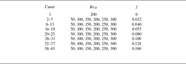


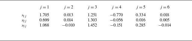

 Q
Q ϖxD/U∞
 ReD=200
 f=0.032
 f=0.160
 ReD=200
 ϖzD/U∞
 Cp=p/(0.5ρU∞2)
 f=0.080
 ReD=200
 t/T=0.25
 t/T=0.5
 t/T=0.75
 Q=20
Q=20 ϖxD/U∞
 X/D=12
 ReD=200
 β=6
β=6 ϕ=45∘
ϕ=45∘
 ReD=200
 ReD=50
 ReD=200
 f=0.080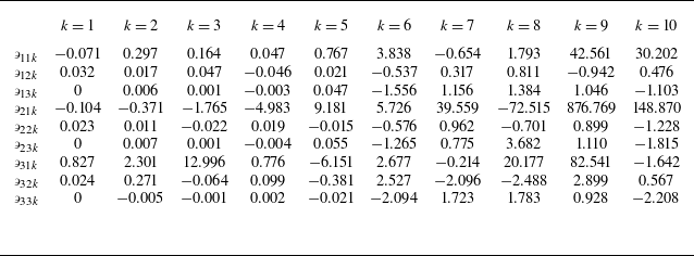

 ReD=150
 f=0.106

 ReD−f
ReD−f CD
CD CL
CL CT
CT f=0.145
 ReD=275
 f=0.028
 ReD=175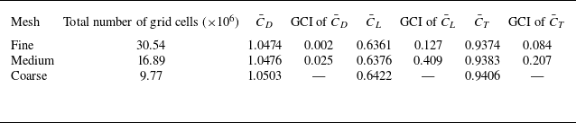
 f=0.080
 ϕ=45∘
ϕ=45∘ ReD=200



