


1. Introduction
Inertial waves are propagating features inside rotating fluids, which are restored by the Coriolis force. They are widely observed in the Earth’s oceans and represent a significant peak in the kinetic energy spectrum (Gonella 1972; Munk Reference Munk1981). In liquid planetary layers, inertial waves can be excited by mechanical forcings and they are thought to be important for orbital and spin evolution of celestial bodies (for a review, see Le Bars, Cébron & Le Gal Reference Le Bars, Cébron and Le Gal2015). Furthermore, inertial modes have been observed in the sun (Hanson, Hanasoge & Sreenivasan Reference Hanson, Hanasoge and Sreenivasan2022; Triana et al. Reference Triana, Guerrero, Barik and Rekier2022) and their discovery has sparked questions about whether these can be used to infer interior solar properties to which acoustic modes – as canonically utilised in helioseismology – are insensitive. Inertial modes have also been detected in $\gamma$
Doradus stars, where they can be used to probe the rotation rate of the convective cores of these stars (Ouazzani et al. Reference Ouazzani, Lignières, Dupret, Salmon, Ballot, Christophe and Takata2020; Saio et al. Reference Saio, Takata, Lee, Li and Van Reeth2021). In most geophysical systems, stratification of the fluid introduces gravity as a second restoring force, generating inertia-gravity waves. Wave-like features in the atmospheres of gas planets are frequently interpreted as such inertia-gravity waves (see Rogers et al. Reference Rogers, Fletcher, Adamoli, Jacquesson, Vedovato and Orton2016; Orton et al. Reference Orton2020 and references therein).
$\gamma$
Doradus stars, where they can be used to probe the rotation rate of the convective cores of these stars (Ouazzani et al. Reference Ouazzani, Lignières, Dupret, Salmon, Ballot, Christophe and Takata2020; Saio et al. Reference Saio, Takata, Lee, Li and Van Reeth2021). In most geophysical systems, stratification of the fluid introduces gravity as a second restoring force, generating inertia-gravity waves. Wave-like features in the atmospheres of gas planets are frequently interpreted as such inertia-gravity waves (see Rogers et al. Reference Rogers, Fletcher, Adamoli, Jacquesson, Vedovato and Orton2016; Orton et al. Reference Orton2020 and references therein).
As all of the examples listed above also include background flows in addition to waves, it is important to understand the interaction between inertial waves, moving on fast time scales, and slowly varying background flows. The effect of a background flow shear on inertia-gravity waves has been studied by researchers in oceanography. Kunze (Reference Kunze1985) describes the propagation of near-inertial waves through geostrophic currents using ray theory. His calculations show a geostrophic shear can reduce the background vorticity to prohibit small-scale near-inertial waves from travelling. On the other hand, he finds that waves excited in regions where the geostrophic shear increases the background vorticity may not be able to exit the shear zone and get trapped inside a jet. A similar problem has been studied by Baruteau & Rieutord (Reference Baruteau and Rieutord2012), who consider inertial wave attractors in spherical shells affected by differential rotation. However, ray theory assumes that the spatial scales of the background shear are large compared with the wavelength of the propagating inertial oscillations. The method cannot describe the propagation of inertial waves inside geostrophic flows on length scales at or below their wavelengths.
Another approach is to use scattering theory to model the interaction between small-scale geostrophic flows – which are treated analogously as a scattering potential in quantum mechanics – and near-inertial wave fields (Olbers Reference Olbers1981). The author considers an example of inertia-gravity waves horizontally entering ocean fronts at different angles, where the fronts are characterised by spatially varying buoyancy fields and geostrophic flows of different widths. Although he finds that waves entering along front generate a stronger scattered far field, insights into the fundamental relations between the scattered field, the length scale of the jets and the characteristics of the incident waves are not examined. Furthermore, the scattering theory only provides insight into the dynamics of the far field away from the sheared region and not close to or inside of it.
Young & Jelloul (Reference Young and Jelloul1997) study the effect of small-scale, geostrophic eddies on near-inertial modes. They find that geostrophic background turbulence introduces a frequency shift in high-wavenumber vertical modes, which are thus dispersed vertically. As a consequence, near-inertial oscillations excited at the ocean’s surface are efficiently transported hundreds of metres in depth within a few weeks time. Relying on an averaging procedure for the wave field, they find that waves are only affected by the geostrophic flow averaged on the length scale of the waves.
While averaging and scattering methods, such as the ones of Olbers (Reference Olbers1981) or Young & Jelloul (Reference Young and Jelloul1997), successfully explain observations of anomalous near-inertial wave propagation due to smaller-scale geostrophic jets or vortices, the fundamental mechanisms of inertial waves interacting with small-scale shear zones are poorly understood. However, from all previous studies, it is apparent that background currents can significantly alter the behaviour of inertial waves and a thorough understanding of the physics involved is crucial for us to comprehend the role of these waves in dynamical, planetary fluid regions.
In this paper, we study inertial wave propagation in a simple quasi-two-dimensional geostrophic shear layer. For this problem, we first present a theory describing the reflection–transmission behaviour of inertial plane waves entering a discrete layer of constant geostrophic shear and arbitrary width. This serves to develop conceptual understanding of the interaction between inertial waves and a shear layer. This calculation is analogous to previous analyses of internal gravity waves interacting with a layer with different buoyancy frequency (Sutherland & Yewchuk Reference Sutherland and Yewchuk2004). We then leverage the results for a discrete layer to find the transmission and reflection behaviour of inertial waves interacting with continuous shear layers of arbitrary horizontal structure. As for the case of internal gravity waves in layered fluids (Belyaev, Quataert & Fuller Reference Belyaev, Quataert and Fuller2015; Sutherland 2016; Bracamontes-Ramirez & Sutherland Reference Bracamontes-Ramirez and Sutherland2024) we solve the inertial wave equation within a stack of thin layers, coupled by interface conditions, to find the total transmission and reflection coefficients.
The fundamental theory and our models are described in § 2. We validate our theoretical calculations via direct numerical simulation using the Dedalus code (Burns et al. Reference Burns, Vasil, Oishi, Lecoanet and Brown2020). The simulation set-up is described in § 3, and we compare the theory and simulations in § 4.
2. Theory and modelling
2.1. General solution for inertial waves in constant geostrophic shear
In a rotating frame of reference, with constant angular velocity $\boldsymbol \varOmega = \varOmega \, \boldsymbol e_z$
the equations of motion for an inviscid and incompressible fluid are the Euler equations
$\boldsymbol \varOmega = \varOmega \, \boldsymbol e_z$
the equations of motion for an inviscid and incompressible fluid are the Euler equations
 \begin{align} &\partial _t \boldsymbol v + 2\varOmega \,\boldsymbol e_z \times \boldsymbol v + (\boldsymbol v \boldsymbol{\cdot }\boldsymbol{\nabla })\,\boldsymbol v = -\frac {1}{\rho _0}\boldsymbol{\nabla }\!p, \\[-12pt]\nonumber \end{align}
 \begin{align} &\hspace{5pc}\boldsymbol{\nabla }\boldsymbol{\cdot }\boldsymbol v = 0, \end{align}
where $\boldsymbol v = (v_x, v_y, v_z)$
is the velocity vector,
$\boldsymbol v = (v_x, v_y, v_z)$
is the velocity vector, $\rho _0$
is a constant density and
$\rho _0$
is a constant density and $p$
is the reduced pressure absorbing the hydrostatic pressure and the centrifugal potential (Greenspan 1968). We are interested in the case where we split up the velocity field into a prescribed geostrophic background flow
$p$
is the reduced pressure absorbing the hydrostatic pressure and the centrifugal potential (Greenspan 1968). We are interested in the case where we split up the velocity field into a prescribed geostrophic background flow $\boldsymbol U_0 = U_0(x)\,\boldsymbol e_y$
and a deviation
$\boldsymbol U_0 = U_0(x)\,\boldsymbol e_y$
and a deviation $\boldsymbol u(x, z, t)$
from this background state:
$\boldsymbol u(x, z, t)$
from this background state: $(\boldsymbol v, p) \rightarrow (\boldsymbol u, p) + (\boldsymbol U_0, p_0)$
. We assume that the background flow and the reduced background pressure
$(\boldsymbol v, p) \rightarrow (\boldsymbol u, p) + (\boldsymbol U_0, p_0)$
. We assume that the background flow and the reduced background pressure $p_0$
themselves satisfy the geostrophic equations
$p_0$
themselves satisfy the geostrophic equations
 \begin{align} &2\varOmega \,\boldsymbol e_z \times \boldsymbol U_0 = -\frac {1}{\rho _0}\boldsymbol{\nabla }\!p_0, \\[-12pt]\nonumber \end{align}
 \begin{align} &\hspace{2pc} \boldsymbol{\nabla }\boldsymbol{\cdot }\boldsymbol U_0 = 0. \end{align}
Furthermore, we make the assumption that all quantities are independent of $y$
, such that we treat a quasi-two-dimensional problem. A schematic of the set-up is shown in figure 1.
$y$
, such that we treat a quasi-two-dimensional problem. A schematic of the set-up is shown in figure 1.
Schematic figure demonstrating the geometry of the problem. Blue arrows denote an example flow $\boldsymbol{U}_{\!0}$
in the
$\boldsymbol{U}_{\!0}$
in the $y$
-direction.
$y$
-direction.

In accordance with the previous assumptions we expect the components of the perturbation $\boldsymbol u$
to possess the structure of a plane wave
$\boldsymbol u$
to possess the structure of a plane wave
 \begin{equation} u_x = \tilde {u}\,\exp {i(k_x\,x + k_z\,z - \omega t)}, \end{equation}
with the horizontal and vertical wavenumbers $k_x$
and
$k_x$
and $k_z$
, respectively, the fixed frequency
$k_z$
, respectively, the fixed frequency $\omega$
and the amplitude
$\omega$
and the amplitude $\tilde {u}$
of the
$\tilde {u}$
of the $x$
-component. The amplitudes of
$x$
-component. The amplitudes of $u_y$
and
$u_y$
and $u_z$
can later be obtained from the polarisation relations. We do not make any assumption on the spatial scales of the background flow
$u_z$
can later be obtained from the polarisation relations. We do not make any assumption on the spatial scales of the background flow $U_0$
or the wave field. We non-dimensionalise the equations with the vertical wavelength of the perturbation
$U_0$
or the wave field. We non-dimensionalise the equations with the vertical wavelength of the perturbation $\lambda _z = {2\pi }/{|k_z|}$
and the rotation rate
$\lambda _z = {2\pi }/{|k_z|}$
and the rotation rate $\varOmega$
using the dimensionless coordinates
$\varOmega$
using the dimensionless coordinates
 \begin{equation} (x', z', t') = \left ( \frac {x}{\lambda _z},\, \frac {z}{\lambda _z},\, t \varOmega \right )\!. \end{equation}
Then the velocities are non-dimensionalised by $\lambda _z\varOmega$
 \begin{equation} \boldsymbol u' = \frac {1}{\lambda _z \varOmega }\boldsymbol u \hspace {0.25cm} \text{and} \hspace {0.25cm} U_0' = \frac {1}{\lambda _z \varOmega } U_0. \end{equation}
We assume the perturbation amplitude is small, implying a small Rossby number $\textit{Ro}=\tilde {u}/(\lambda _z \varOmega )\ll 1$
, such that the nonlinear term
$\textit{Ro}=\tilde {u}/(\lambda _z \varOmega )\ll 1$
, such that the nonlinear term $\boldsymbol u \boldsymbol{\cdot }\boldsymbol{\nabla }\boldsymbol u$
is negligible. Note that, in the dimensionless formulation, the amplitude of the
$\boldsymbol u \boldsymbol{\cdot }\boldsymbol{\nabla }\boldsymbol u$
is negligible. Note that, in the dimensionless formulation, the amplitude of the $x$
-component of the velocity is the Rossby number. We define the dimensionless pressure as
$x$
-component of the velocity is the Rossby number. We define the dimensionless pressure as
 \begin{equation} p' = \frac {1}{\rho _0\,(\lambda _z \varOmega )^2}\,p. \end{equation}
Then the dimensionless equations are
 \begin{align} &\partial _t' \boldsymbol u' + 2\boldsymbol e_z \times \boldsymbol u' + u'_x\, \partial _x' U_0'\, \boldsymbol e_y = -\boldsymbol{\nabla }\!p', \\[-12pt]\nonumber \end{align}
 \begin{align} &\hspace{4pc} \boldsymbol{\nabla }' \boldsymbol{\cdot }\boldsymbol u' = 0. \end{align}
In all further considerations, the prime denoting a dimensionless quantity will be omitted and all variables are dimensionless unless stated otherwise.
From (2.9), we can see that the advection term represents a straining of the perturbation $\boldsymbol u$
in the
$\boldsymbol u$
in the $y$
-direction. Note that, since we assume
$y$
-direction. Note that, since we assume $\boldsymbol u$
to be independent of
$\boldsymbol u$
to be independent of $y$
, we do not consider advection of the perturbation by the background flow.
$y$
, we do not consider advection of the perturbation by the background flow.
Eliminating the pressure, taking $\partial _t \boldsymbol{\nabla }\times (\boldsymbol{\nabla }\times \text{(2.9)})$
(Davidson Reference Davidson2013), the Euler equations take the form
$\partial _t \boldsymbol{\nabla }\times (\boldsymbol{\nabla }\times \text{(2.9)})$
(Davidson Reference Davidson2013), the Euler equations take the form
 \begin{equation} \partial ^2_t \boldsymbol{\nabla} ^2 \boldsymbol u + (2\,\boldsymbol e_z \boldsymbol{\cdot }\boldsymbol{\nabla })^2\boldsymbol u + \boldsymbol S(u_x\,\partial _x U_0) = 0. \end{equation}
This wave equation includes the new straining term represented by the operator
 \begin{equation} \boldsymbol S = \begin{pmatrix} 2(\boldsymbol e_z \boldsymbol{\cdot }\boldsymbol{\nabla })\partial _z \\[5pt] \big(\partial _x^2 + \partial _z^2\big)\partial _t \\[5pt] -2(\boldsymbol e_z \boldsymbol{\cdot }\boldsymbol{\nabla })\partial _x) \end{pmatrix} \end{equation}
acting on $u_x\, \partial _x U_0$
and it is valid for arbitrary geostrophic flows
$u_x\, \partial _x U_0$
and it is valid for arbitrary geostrophic flows $U_0(x)$
.
$U_0(x)$
.
Now consider the case of constant geostrophic shear, $\partial _x U_0 = \text{const}$
. Substituting the plane wave ansatz (2.5) into the first component of (2.11) leads to a modified inertial waves dispersion relation
$\partial _x U_0 = \text{const}$
. Substituting the plane wave ansatz (2.5) into the first component of (2.11) leads to a modified inertial waves dispersion relation
 \begin{equation} k_x = \pm \gamma k_z, \quad \gamma = \sqrt {\frac {4}{\omega ^2} + \frac {2\,\partial _x U_0}{\omega ^2}-1}. \end{equation}
For $\partial _x U_0 = 0$
, we recover the classical inertial wave dispersion relation, with propagating waves for
$\partial _x U_0 = 0$
, we recover the classical inertial wave dispersion relation, with propagating waves for $|\omega | \lt 2$
. A non-zero background shear
$|\omega | \lt 2$
. A non-zero background shear $\partial _x U_0$
controls the maximum frequency
$\partial _x U_0$
controls the maximum frequency
 \begin{equation} \omega _{\textit{max}} = 2 \sqrt {1 + \frac {\partial _x U_0}{2}} \end{equation}
for which $\gamma$
is real and classical wave propagation is still possible, as already demonstrated by Kunze (Reference Kunze1985). If the wave frequency
$\gamma$
is real and classical wave propagation is still possible, as already demonstrated by Kunze (Reference Kunze1985). If the wave frequency $\omega$
exceeds this value,
$\omega$
exceeds this value, $\gamma$
and
$\gamma$
and $k_x$
become imaginary and the phases only propagate vertically while the entire wave decays exponentially in the horizontal direction. These are evanescent inertial waves, as studied by Nosan et al. (Reference Nosan, Burmann, Davidson and Noir2021).
$k_x$
become imaginary and the phases only propagate vertically while the entire wave decays exponentially in the horizontal direction. These are evanescent inertial waves, as studied by Nosan et al. (Reference Nosan, Burmann, Davidson and Noir2021).
A physical interpretation of the effect of the background shear on the maximum wave frequency is the following. A positive value of $\partial _x U_0$
represents a positive background vorticity, which enhances the restoring force of the Coriolis acceleration. A stronger restoring force supports higher frequencies in an oscillatory system and thus,
$\partial _x U_0$
represents a positive background vorticity, which enhances the restoring force of the Coriolis acceleration. A stronger restoring force supports higher frequencies in an oscillatory system and thus, $\omega _{\textit{max}} \gt 2$
. In contrast, a negative background vorticity weakens the restoring force, which fails to support high-frequency motion, where
$\omega _{\textit{max}} \gt 2$
. In contrast, a negative background vorticity weakens the restoring force, which fails to support high-frequency motion, where $\omega _{\textit{max}} \lt 2$
.
$\omega _{\textit{max}} \lt 2$
.
For a given vertical wavenumber $k_z$
and wave frequency
$k_z$
and wave frequency $\omega$
, we have the polarisation relations
$\omega$
, we have the polarisation relations
 \begin{equation} u_y = -i\frac {2 + \partial _x U_0}{\omega }\,u_x \hspace {0.5cm} \text{and} \hspace {0.5cm} u_z = -\frac {k_x}{k_z}\,u_x. \end{equation}
Finally, we can obtain the pressure $p$
from integrating the third component of the momentum (2.9) as
$p$
from integrating the third component of the momentum (2.9) as
 \begin{equation} p(x,z) = - \frac {\omega \, k_x}{k_z^2}\,u_x. \end{equation}
Thus, we obtain a full analytical description of inertial waves and evanescent inertial waves inside any constant geostrophic shear $\partial _x U_0$
.
$\partial _x U_0$
.
2.2. Interaction of inertial waves with a localised geostrophic shear layer
We now consider inertial waves propagating into a localised layer of constant geostrophic shear, as depicted in figure 2.
Model of plane inertial waves interacting with a single layer of constant shear. The wave vectors $\boldsymbol k_{i}^{(r)} = (k_{i,x}^{(r)},\, k_{i,z}^{(r)})$
are indicated schematically.
$\boldsymbol k_{i}^{(r)} = (k_{i,x}^{(r)},\, k_{i,z}^{(r)})$
are indicated schematically.

We prescribe the incident wave with amplitude, wavenumber and frequency $(\tilde {u}_0, \boldsymbol k_0, \omega _0)$
, which we assume to be known. Our aim is to describe the reflected waves
$(\tilde {u}_0, \boldsymbol k_0, \omega _0)$
, which we assume to be known. Our aim is to describe the reflected waves $(\tilde {u}_{0}^{r}, \boldsymbol k_{0}^{r}, \omega _{0}^{r})$
and
$(\tilde {u}_{0}^{r}, \boldsymbol k_{0}^{r}, \omega _{0}^{r})$
and $(\tilde {u}_{1}^{r}, \boldsymbol k_{1}^{r}, \omega _{1}^{r})$
, and the transmitted waves
$(\tilde {u}_{1}^{r}, \boldsymbol k_{1}^{r}, \omega _{1}^{r})$
, and the transmitted waves $(\tilde {u}_1, \boldsymbol k_1, \omega _1)$
and
$(\tilde {u}_1, \boldsymbol k_1, \omega _1)$
and $(\tilde {u}_2, \boldsymbol k_2, \omega _2)$
. For this, we follow a common procedure for inertial/internal waves at diverse interfaces (e.g. Phillips Reference Phillips1963; Sutherland & Yewchuk Reference Sutherland and Yewchuk2004; Belyaev et al. Reference Belyaev, Quataert and Fuller2015): we impose continuity conditions for the pressure and the flow component normal to the interfaces at
$(\tilde {u}_2, \boldsymbol k_2, \omega _2)$
. For this, we follow a common procedure for inertial/internal waves at diverse interfaces (e.g. Phillips Reference Phillips1963; Sutherland & Yewchuk Reference Sutherland and Yewchuk2004; Belyaev et al. Reference Belyaev, Quataert and Fuller2015): we impose continuity conditions for the pressure and the flow component normal to the interfaces at $x = 0$
and
$x = 0$
and $x = -\Delta x$
 \begin{align} u_{1,x} + u_{1,x}^{r} &= u_{2,x} \,\, \qquad \qquad \vert _{x = -\Delta x}, \\[-12pt]\nonumber \end{align}
 \begin{align} p_1 + p_{1}^{r} &= p_2 \quad \qquad \qquad \vert _{x = -\Delta x}, \\[-12pt]\nonumber \end{align}
 \begin{align} u_{0,x} + u_{0,x}^{r} &= u_{1,x} + u_{1,x}^{r} \,\,\,\quad \vert _{x = 0}, \\[-12pt]\nonumber \end{align}
 \begin{align} p_0 + p_{0}^{r} &= p_1 + p_{1}^{r} \quad \qquad \vert _{x = 0}. \end{align}
As the problem is autonomous in $z$
and
$z$
and $t$
, all waves must possess the same vertical wavenumber
$t$
, all waves must possess the same vertical wavenumber $k_z$
and the same frequency
$k_z$
and the same frequency $\omega$
. This means the only free variables left are the horizontal wavenumbers
$\omega$
. This means the only free variables left are the horizontal wavenumbers $k_{i,x}^{(r)}$
and the amplitudes
$k_{i,x}^{(r)}$
and the amplitudes $\tilde {u}_{i}^{(r)}$
(
$\tilde {u}_{i}^{(r)}$
( $i = 1,2$
and the superscript ‘
$i = 1,2$
and the superscript ‘ $(r)$
’ stands for both transmitted and reflected wave).
$(r)$
’ stands for both transmitted and reflected wave).
For a given strength of the geostrophic shear $\partial _xU_0=\delta \omega$
and imposed (
$\partial _xU_0=\delta \omega$
and imposed ( $\tilde {u}_0, k_{x,0}, k_{z},\,\omega$
) by the incident wave, we can calculate the horizontal wavenumbers in every part of the domain using (2.13). This leaves us – by inserting the ansatz (2.5) into the continuity conditions (2.17)(2.20) – with four linear equations for four unknown amplitudes
$\tilde {u}_0, k_{x,0}, k_{z},\,\omega$
) by the incident wave, we can calculate the horizontal wavenumbers in every part of the domain using (2.13). This leaves us – by inserting the ansatz (2.5) into the continuity conditions (2.17)(2.20) – with four linear equations for four unknown amplitudes
 \begin{align} \tilde {u}_{1}\, \exp {(-ik_{1,x}\,\Delta x)} + \tilde {u}_{1}^{r}\, \exp {(-ik_{1,x}^{r}\,\Delta x)} \, &= \,\tilde {u}_{2}\, \exp {(-ik_{2,x}\,\Delta x)}, \\[-12pt]\nonumber\end{align}
 \begin{align} k_{1,x}\tilde {u}_{1}\, \exp {(-ik_{1,x}\,\Delta x)} + k_{1,x}^{r}\tilde {u}_{1}^{r}\, \exp {(-ik_{1,x}^{r}\,\Delta x)} \, &= \, k_{2,x}\tilde {u}_{2}\, \exp {(-ik_{2,x}\,\Delta x)}, \\[-12pt]\nonumber\end{align}
 \begin{align} \tilde {u}_{0} + \tilde {u}_{0}^{r} \, &= \, \tilde {u}_{1} + \tilde {u}_{1}^{r}, \\[-12pt]\nonumber\end{align}
 \begin{align} k_{0,x}\tilde {u}_{0} + k_{0,x}^{r}\tilde {u}_{0}^{r} \, &= \, k_{1,x}\tilde {u}_{1} + k_{1,x}^{r}\tilde {u}_{1}^{r}.\end{align}
Solving for the unknown amplitudes we obtain
 \begin{align} &\tilde {u}_{0}^{r} = \alpha _0 \,\tilde {u}_0, \\[-12pt]\nonumber \end{align}
 \begin{align} &\tilde {u}_{1} = \beta _0 \, \tilde {u}_0, \\[-12pt]\nonumber \end{align}
 \begin{align} &\tilde {u}_{1}^{r} = \alpha _1\,\tilde {u}_1, \\[-12pt]\nonumber \end{align}
 \begin{align} &\tilde {u}_2 = \beta _1\,\tilde {u}_1, \end{align}
with
 \begin{align} \alpha _1 &= \quad \frac {k_{2,x} - k_{1,x}}{k_{1,x}^{r} - k_{2,x}}\exp [-i(k_{1,x} - k_{1,x}^{r})\Delta x], \\[-12pt]\nonumber\end{align}
 \begin{align} \beta _1 &= \quad \left (\exp [-ik_{1,x}\Delta x] + \alpha _1\exp [-ik_{1,x}^{r}\Delta x]\right )\exp [ik_{2,x}\Delta x], \\[-12pt]\nonumber\end{align}
 \begin{align} \alpha _0 &= \quad \frac {k_{1,x} - k_{0,x} + \alpha _1(k_{1,x}^{r} - k_{0,x})}{k_{0,x}^{r} - k_{1,x} + \alpha _1(k_{0,x}^{r} - k_{1,x}^{r})}, \\[-12pt]\nonumber\end{align}
 \begin{align} \beta _0 &= \quad \frac {1 + \alpha _0}{1 + \alpha _1}.\end{align}
Note that, for the case of an unperturbed background vorticity, i.e. $\delta \omega = 0$
, we must recover the uniform propagation of inertial waves, i.e.
$\delta \omega = 0$
, we must recover the uniform propagation of inertial waves, i.e. $\alpha _1 = \alpha _0 = 0$
and
$\alpha _1 = \alpha _0 = 0$
and $\beta _1 = \beta _0 = 1$
. This allows us to determine the signs of the horizontal wave vectors. As their magnitudes are equal, to satisfy
$\beta _1 = \beta _0 = 1$
. This allows us to determine the signs of the horizontal wave vectors. As their magnitudes are equal, to satisfy $\alpha _0=0$
we have
$\alpha _0=0$
we have
 \begin{equation} \text{sign}(k_{1,x}) = \text{sign}(k_{0,x}) \hspace {0.5cm} \text{and} \hspace {0.5cm} \text{sign}(k_{0,x}^{r}) = -\text{sign}(k_{0,x}), \end{equation}
and to satisfy $\alpha _1=0$
we have
$\alpha _1=0$
we have
 \begin{equation} \text{sign}(k_{2,x}) = \text{sign}(k_{0,x}) \hspace {0.5cm} \text{and} \hspace {0.5cm} \text{sign}(k_{1,x}^{r}) = -\text{sign}(k_{0,x}). \end{equation}
In other words, we obtain the expected result that the transmitted phases travel in the same horizontal direction as the incoming waves, while the reflected phases travel in the opposite direction.
At this point, we introduce the concept of critical shear. We define it as the value $\partial _x U_0 = \delta \omega _c$
below which
$\partial _x U_0 = \delta \omega _c$
below which $\gamma$
becomes imaginary inside the shear layer for an inertial wave of frequency
$\gamma$
becomes imaginary inside the shear layer for an inertial wave of frequency $\omega$
. We can obtain this value by solving (2.14) for
$\omega$
. We can obtain this value by solving (2.14) for $\partial _x U_0$
and setting
$\partial _x U_0$
and setting $\omega _{\textit{max}} = \omega$
 \begin{equation} \delta \omega _c = \frac {\omega ^2}{2} - 2. \end{equation}
For our problem, this critical shear is a negative number (as $|\omega | \leqslant 2$
) and we define shear layers where
$|\omega | \leqslant 2$
) and we define shear layers where $\delta \omega \lt \delta \omega _c$
as supercritical shear layers.
$\delta \omega \lt \delta \omega _c$
as supercritical shear layers.
Hence, in supercritical shear layers $k_x$
is imaginary. As we expect evanescent inertial waves to always decay towards the inside of impenetrable media, we impose
$k_x$
is imaginary. As we expect evanescent inertial waves to always decay towards the inside of impenetrable media, we impose
 \begin{equation} k_{1,x} = -i|\gamma k_z| \hspace {0.5cm} \text{and} \hspace {0.5cm} k_{1,x}^{r} = - k_{1,x}, \hspace {0.5cm} \text{if} \hspace {0.3cm} \delta \omega \lt \delta \omega _c \lt 0. \end{equation}
This ensures that the wave $\boldsymbol u_1$
, transmitted into the layer of supercritical shear, decays in the negative
$\boldsymbol u_1$
, transmitted into the layer of supercritical shear, decays in the negative $x$
-direction, i.e. towards the inside of the layer.
$x$
-direction, i.e. towards the inside of the layer.
2.3. Interaction with arbitrary piecewise-constant geostrophic shear profiles
Let us now consider the scenario where an inertial wave propagates into a series of shear layers, each with width $\Delta x$
and shear strength
$\Delta x$
and shear strength $\delta \omega _i$
, i.e. a piecewise-constant shear profile, as illustrated in figure 3. As we shall see, by adjusting the width and amplitudes of the shear layers, we can use such a model to approximate arbitrary geostrophic shear profiles.
$\delta \omega _i$
, i.e. a piecewise-constant shear profile, as illustrated in figure 3. As we shall see, by adjusting the width and amplitudes of the shear layers, we can use such a model to approximate arbitrary geostrophic shear profiles.
Model of multiple consecutive shear layers traversed by plane inertial waves. This extends the model of a single layer and two interfaces to a case of $N$
interfaces.
$N$
interfaces.

Imposing the continuity conditions for $p$
and
$p$
and $u_x$
at each interface, we obtain the following recursive relations at the
$u_x$
at each interface, we obtain the following recursive relations at the $n$
th interface (
$n$
th interface ( $n = 0,\ldots , N-1$
):
$n = 0,\ldots , N-1$
):
 \begin{align} \begin{split} \tilde {u}_{n+1}\,a_{n+1} + \tilde {u}_{n+1}^{r}\,a_{n+1}^{r} &= \tilde {u}_{n}\,b_{n} + \tilde {u}_{n}^{r}\,b_{n}^{r}, \\[5pt] k_{n+1, x}\tilde {u}_{n+1}\,a_{n+1} + k_{n+1,x}^{r}\tilde {u}_{n+1}^{r}\,a_{n+1}^{r} &= k_{n,x}\tilde {u}_{n}\,b_{n} + k_{n,x}^{r}\tilde {u}_{n}^{r}\,b_{n}^{r}, \end{split} \end{align}
where
 \begin{align} \begin{split} a_{n}^{(r)} &= \exp {[(-ik_{n,x}^{(r)})\,(n-1)\Delta x]} ,\\ b_{n}^{(r)} &= \exp {[(-ik_{n,x}^{(r)})\,n\Delta x]} ,\\ \end{split} \end{align}
are phase factors resulting from the offset of the $n$
th interface from
$n$
th interface from $x = 0$
.
$x = 0$
.
Recalling that the incident amplitude is $\tilde {u}_0 = \textit{Ro}$
and setting
$\tilde {u}_0 = \textit{Ro}$
and setting $\tilde {u}_{N}^{r} = 0$
, we can formulate the following system of equations:
$\tilde {u}_{N}^{r} = 0$
, we can formulate the following system of equations:
 \begin{align} \begin{pmatrix} 1 & 0 & 0 & {\cdots} & 0 & 0 \\[3pt] -b_0 & -b_{0}^{r} & a_1 & a_{1}^{r} & 0 & \vdots \\[3pt] -k_{0,x}\,b_0 & -k_{0,x}^{r}\,b_{0}^{r} & k_{1,x}\,a_{1} & k_{1,x}^{r}\,a_{1}^{r} & 0 & \vdots \\[3pt] 0 & -b_1 & -b_{1}^{r} & a_2 & a_{2}^{r} & \vdots \\[3pt] 0 & -k_{1,x}\,b_1 & -k_{1,x}^{r}\,b_{1}^{r} & k_{2,x}\,a_{2} & k_{2,x}^{r}\,a_{2}^{r} & \vdots \\[3pt] \vdots & 0 & \ddots & \ddots & & \\[3pt] \vdots & & -b_{N-1} & -b_{N-1}^{r} & a_N & a_{N}^{r} \\[3pt] \vdots & & -k_{N-1,x}\,b_{N-1} & -k_{N-1,x}^{r}\,b_{N-1}^{r} & k_{N,x}\,a_{N} & k_{N,x}^{r}\,a_{N}^{r} \\[5pt] 0 & {\cdots} & 0 & 0 & 0 & 1 \end{pmatrix} \begin{pmatrix} \tilde {u}_0 \\[6pt] \tilde {u}_{0}^{r} \\[6pt] \tilde {u}_1 \\[6pt] \tilde {u}_{1}^{r} \\[6pt] \vdots \\[4pt] \tilde {u}_{N-1} \\[6pt] \tilde {u}_{N-1}^{r} \\[6pt] \tilde {u}_N \\[6pt] \tilde {u}_{N}^{r} \end{pmatrix} = \begin{pmatrix} \textit{Ro} \\[6pt] 0 \\[6pt] 0 \\[6pt] 0 \\[6pt] \vdots \\[4pt] 0 \\[6pt] 0 \\[6pt] 0 \\[2pt] 0 \end{pmatrix}\!. \end{align}
We solve this system and obtain the reflected amplitude $\tilde {u}_{0}^{r}$
and the transmitted amplitude
$\tilde {u}_{0}^{r}$
and the transmitted amplitude $\tilde {u}_N$
.
$\tilde {u}_N$
.
Any continuous geostrophic profile can be approximated by this type of piecewise-constant shear profile. As an example for our problem, consider the following Gaussian shear profile:
 \begin{equation} \partial _x U_0(x) = \delta \omega \, \exp {\left(\!-\frac {x^2}{2\sigma _0^2}\right)}\!. \end{equation}
Our strategy of discretising this profile is to define an interval $[x_l, x_r] = [-4\,\sigma _0, 4\,\sigma _0]$
outside of which we assume
$[x_l, x_r] = [-4\,\sigma _0, 4\,\sigma _0]$
outside of which we assume $\partial _x U_0(x) = 0$
. We define
$\partial _x U_0(x) = 0$
. We define $N$
equidistant interfaces within this interval, creating
$N$
equidistant interfaces within this interval, creating $N-1$
layers of equal thickness
$N-1$
layers of equal thickness $\Delta x$
. We define the
$\Delta x$
. We define the $\delta \omega _i$
(
$\delta \omega _i$
( $i = 1,\ldots , N-1$
) as the mean value of
$i = 1,\ldots , N-1$
) as the mean value of $\partial _x U_0$
within each layer. In figure 4 we show an example discretisation with
$\partial _x U_0$
within each layer. In figure 4 we show an example discretisation with $N=18$
. However, to obtain a better approximation of the profile we can increase
$N=18$
. However, to obtain a better approximation of the profile we can increase $N$
arbitrarily. For convenience, we will henceforth denote the transmitted wave with a superscript ‘
$N$
arbitrarily. For convenience, we will henceforth denote the transmitted wave with a superscript ‘ $t$
’ when comparing the piecewise-constant model with the continuous case: e.g.
$t$
’ when comparing the piecewise-constant model with the continuous case: e.g. $\tilde {u}_N \rightarrow \tilde {u}^t$
.
$\tilde {u}_N \rightarrow \tilde {u}^t$
.
(a) Segmentation of a Gaussian shear profile using $N = 18$
interfaces. (b) The flow profile corresponding to the shear profile, i.e. a shear zone in the shape of an erfc centred around
$N = 18$
interfaces. (b) The flow profile corresponding to the shear profile, i.e. a shear zone in the shape of an erfc centred around $x = 0$
. The accurate shear and flow profiles are shown in grey dashed lines, while the approximate profiles are represented by the black solid lines.
$x = 0$
. The accurate shear and flow profiles are shown in grey dashed lines, while the approximate profiles are represented by the black solid lines.

Finally, the calculation described above assumes the first shear layer is at $x=0$
. However, the calculation of the reflection and transmission coefficients is independent of the position of the first shear layer, so the same approach can be used if the first shear layer is at another position (e.g.
$x=0$
. However, the calculation of the reflection and transmission coefficients is independent of the position of the first shear layer, so the same approach can be used if the first shear layer is at another position (e.g. $x_r$
as in figure 4). Such a translation simply requires a change of the phase factors
$x_r$
as in figure 4). Such a translation simply requires a change of the phase factors $a_{n}^{(r)}$
and
$a_{n}^{(r)}$
and $b_{n}^{(r)}$
.
$b_{n}^{(r)}$
.
3. Numerical methods
To validate our theory we run direct numerical simulations (DNS) using Dedalus (Burns et al. Reference Burns, Vasil, Oishi, Lecoanet and Brown2020). Dedalus is a spectral solver for partial differential equations. We use it to solve the (2.9) and (2.10) by expanding all variables as a Chebyshev series in $x$
and Fourier series in
$x$
and Fourier series in $z$
. Dedalus uses the generalised
$z$
. Dedalus uses the generalised $\tau$
method to apply boundary conditions and ultraspherical polynomials as test functions, resulting in an optimally sparse representation of derivatives. We use a two-stage mixed implicit–explicit time stepping scheme (Ascher, Ruuth & Spiteri Reference Ascher, Ruuth and Spiteri1997) with constant time-step size of 0.1, where the
$\tau$
method to apply boundary conditions and ultraspherical polynomials as test functions, resulting in an optimally sparse representation of derivatives. We use a two-stage mixed implicit–explicit time stepping scheme (Ascher, Ruuth & Spiteri Reference Ascher, Ruuth and Spiteri1997) with constant time-step size of 0.1, where the $u_x\partial _xU_0\boldsymbol{e}_y$
term and all forcing/damping terms are treated explicitly, and the remaining terms are treated implicitly. In the spectral expansion we utilise both
$u_x\partial _xU_0\boldsymbol{e}_y$
term and all forcing/damping terms are treated explicitly, and the remaining terms are treated implicitly. In the spectral expansion we utilise both $1024$
Chebyshev polynomials and
$1024$
Chebyshev polynomials and $1024$
Fourier modes for a domain of size
$1024$
Fourier modes for a domain of size $40 \times 30$
. The explicit terms are evaluated on a grid with 1024 grid points in both
$40 \times 30$
. The explicit terms are evaluated on a grid with 1024 grid points in both $x$
and
$x$
and $z$
.
$z$
.
We specify a set of boundary and initial conditions in a typical set up suited for the reflection–transmission problem for inertial waves, which is shown in figure 5.
Typical set up for the DNS using Dedalus. A shear layer is in the middle of the domain. Energy is injected on the right boundary using the source function $F$
– a sine wave modulated by a Gaussian envelope
$F$
– a sine wave modulated by a Gaussian envelope $E_{\!F}$
. A sponge layer
$E_{\!F}$
. A sponge layer $D$
at the top acts as an energy sink.
$D$
at the top acts as an energy sink.

We excite the waves on the right boundary by imposing
 \begin{equation} u_x(x = 20, z, t) = F(z,t) = \textit{Ro}\, \exp {\left (-\frac {(z-z_\omega )^2}{2d_\omega ^2}\right )}\, \sin (k_z z - \omega t), \end{equation}
where $z_\omega = -7.5$
and
$z_\omega = -7.5$
and $\textit{Ro} = 0.01$
. We choose the vertical wavelength
$\textit{Ro} = 0.01$
. We choose the vertical wavelength $\lambda _z=1$
such that
$\lambda _z=1$
such that $k_z=2\pi$
. The extent of the source region is chosen as
$k_z=2\pi$
. The extent of the source region is chosen as $d_\omega = 2$
. We furthermore always impose the frequency
$d_\omega = 2$
. We furthermore always impose the frequency $\omega = 1.8$
.
$\omega = 1.8$
.
We use a no-penetration boundary condition on the left boundary, i.e.
 \begin{equation} u_x(x = -20, z, t) = 0, \end{equation}
such that both right and left boundaries are reflecting. The top and bottom boundaries are periodic. As an initial condition we choose
 \begin{equation} \boldsymbol u(\boldsymbol x, t = 0) = p(\boldsymbol x, t = 0) = 0. \end{equation}
To avoid a steady increase of energy in the system, we place a sponge layer at the top of the domain by adding an extra damping term $-\boldsymbol u D(z)$
on the right-hand side of the momentum (2.11), with
$-\boldsymbol u D(z)$
on the right-hand side of the momentum (2.11), with
 \begin{equation} D(z) = \frac {1}{2}\left [\tanh {\left (\frac {z - z_D}{d_{\!D}}\right )} + 1\right ]\!. \end{equation}
Here, $z_D = 12.75$
is the vertical position of the sponge layer with width
$z_D = 12.75$
is the vertical position of the sponge layer with width $d_{\!D} = 0.75$
. Although
$d_{\!D} = 0.75$
. Although $D$
is not a periodic function, we do not expect any significant effect on our results caused by its slight misrepresentation in the Fourier basis. Only waves travelling downward or through the layer would be affected. To be sure, we have performed a single simulation for a larger domain and a periodic function, i.e. by adding a second absorbing layer at
$D$
is not a periodic function, we do not expect any significant effect on our results caused by its slight misrepresentation in the Fourier basis. Only waves travelling downward or through the layer would be affected. To be sure, we have performed a single simulation for a larger domain and a periodic function, i.e. by adding a second absorbing layer at $z = -45$
(the increase in domain size is to prevent an interference of the lower layer with the source domain), obtaining equivalent results to those when using the non-periodic sponge layer.
$z = -45$
(the increase in domain size is to prevent an interference of the lower layer with the source domain), obtaining equivalent results to those when using the non-periodic sponge layer.
We run our simulations until $t = 800$
in order to reach a steady wave pattern. Typically, one simulation takes 20 min, running on four cores of a ‘Core i9-14900KF’ produced by Intel.
$t = 800$
in order to reach a steady wave pattern. Typically, one simulation takes 20 min, running on four cores of a ‘Core i9-14900KF’ produced by Intel.
While our analytic theory is for plane waves, the simulations are of wave beams (see, e.g. Le Bars & Lecoanet Reference Le Bars and Lecoanet2020). However, in the centre of the beams we assume the inertial waves behave as plane waves and will thus consider the central peak of the beams for a comparison with our theory.
The kinetic energy density of a wave field is defined as
 \begin{equation} e_{\textit{kin}} = \frac {1}{2} \textit{Re}(\boldsymbol u) \boldsymbol{\cdot } \textit{Re}(\boldsymbol u). \end{equation}
In regions of zero shear (for $\partial _x U_0 = 0$
) the kinetic energy of the plane inertial waves is
$\partial _x U_0 = 0$
) the kinetic energy of the plane inertial waves is
 \begin{equation} e_{\textit{kin}} = |\tilde {u}|^2\frac {2\varOmega ^2}{\omega ^2}. \end{equation}
As we impose $u_{0,x}$
on the right boundary with a peak amplitude of
$u_{0,x}$
on the right boundary with a peak amplitude of $\textit{Ro} = 0.01$
, the peak kinetic energy of the incident wave will always be
$\textit{Ro} = 0.01$
, the peak kinetic energy of the incident wave will always be
 \begin{equation} e_{\textit{kin},0} = \textit{Ro}^2\frac {2\varOmega ^2}{\omega ^2} \approx 6.17\times 10^{-5}. \end{equation}
We compare the transmitted and reflected waves with our analytic predictions in terms of the transmitted and reflected kinetic energy.
To estimate the kinetic energy in the DNS we proceed as follows. Given a geostrophic shear localised near $x=0$
, we plot the kinetic energy (3.6) along two vertical lines at
$x=0$
, we plot the kinetic energy (3.6) along two vertical lines at $x=10$
and
$x=10$
and $x=-10$
in the incident and transmitted domains, respectively (see figure 6). The first peak at
$x=-10$
in the incident and transmitted domains, respectively (see figure 6). The first peak at $x = 10$
provides the kinetic energy
$x = 10$
provides the kinetic energy $e_{\textit{kin},0}$
in the centre of the incident beam and the second one the kinetic energy in the centre of the reflected beam,
$e_{\textit{kin},0}$
in the centre of the incident beam and the second one the kinetic energy in the centre of the reflected beam, $e_{\textit{kin},0}^{r}$
. The maximum of the profile at
$e_{\textit{kin},0}^{r}$
. The maximum of the profile at $x = -10$
provides the kinetic energy
$x = -10$
provides the kinetic energy $e_{\textit{kin},2}$
of the transmitted wave.
$e_{\textit{kin},2}$
of the transmitted wave.
(a) Kinetic energy field – taking the square root allows for less discrepancy between strong and weak signals. The red and blue line show the profiles along which we measure the kinetic energy. (b) Vertical profiles of the kinetic energy.

4. Results and discussion
4.1. Localised ‘ideal’ shear layer
We first compare our theory with the simulations in the case of the single discrete shear layer. In figure 7(a) we show a map of the energy reflection coefficient $({e_{\textit{kin},0}^{r}}/{e_{\textit{kin},0}})$
for varying thicknesses and strengths of the shear layer. We also plot three profiles of reflection and transmission coefficients at either fixed
$({e_{\textit{kin},0}^{r}}/{e_{\textit{kin},0}})$
for varying thicknesses and strengths of the shear layer. We also plot three profiles of reflection and transmission coefficients at either fixed $\delta \omega$
or fixed
$\delta \omega$
or fixed $\Delta x$
in figure 7 (panels b, c and d). Because this problem has a discontinuity in the background shear, the solutions are also expected to be discontinuous, and hence have spectral representations which converge poorly (errors which scale like
$\Delta x$
in figure 7 (panels b, c and d). Because this problem has a discontinuity in the background shear, the solutions are also expected to be discontinuous, and hence have spectral representations which converge poorly (errors which scale like $1/N$
) with resolution
$1/N$
) with resolution $N$
. Nevertheless our resolution
$N$
. Nevertheless our resolution $N=1024$
is sufficient that the simulations (symbols) agree well with the theory (solid lines).
$N=1024$
is sufficient that the simulations (symbols) agree well with the theory (solid lines).
Based on the results of Kunze (Reference Kunze1985), ray tracing predicts refraction of inertial waves when encountering subcritical shear values $\delta \omega \gt \delta \omega _c$
and total reflection on supercritical regions. In this respect, we observe two interesting features: (i) Our theory predicts significant back scattering of energy even for subcritical shear layers. (ii) Even for supercritical shear values, the reflection coefficient vanishes for thin enough layers.
$\delta \omega \gt \delta \omega _c$
and total reflection on supercritical regions. In this respect, we observe two interesting features: (i) Our theory predicts significant back scattering of energy even for subcritical shear layers. (ii) Even for supercritical shear values, the reflection coefficient vanishes for thin enough layers.
Predicted and measured reflection and transmission coefficients in the case of a single shear layer. (a) Map of the predicted reflection coefficient using the theoretical model for various values of the shear layer thickness $\Delta x$
and shear values
$\Delta x$
and shear values $\delta \omega$
. The critical shear
$\delta \omega$
. The critical shear $\delta \omega _c$
is represented by the dashed line, below which ray theory predicts total reflection. We choose three profiles, represented by white lines, along which we plot the reflection and transmission coefficients in the remaining panels: (b) we keep the layer width constant at
$\delta \omega _c$
is represented by the dashed line, below which ray theory predicts total reflection. We choose three profiles, represented by white lines, along which we plot the reflection and transmission coefficients in the remaining panels: (b) we keep the layer width constant at $\Delta x = 1$
and vary the shear strength
$\Delta x = 1$
and vary the shear strength $\delta \omega$
, (c) and (d) we keep
$\delta \omega$
, (c) and (d) we keep $\delta \omega$
constant at −0.2 and −0.5, respectively, and vary
$\delta \omega$
constant at −0.2 and −0.5, respectively, and vary $\Delta x$
. Solid lines represent theoretical predictions and crosses represent measured values from the DNS.
$\Delta x$
. Solid lines represent theoretical predictions and crosses represent measured values from the DNS.

Regarding the former observation, (2.31) shows that any difference between $k_{x,1}$
and
$k_{x,1}$
and $k_{x,0}$
gives a non-zero reflection coefficient. This is because the pressure variation associated with inertial waves is related to the product
$k_{x,0}$
gives a non-zero reflection coefficient. This is because the pressure variation associated with inertial waves is related to the product $k_x \, \tilde {u}_x$
, which decreases for increasingly horizontal waves (smaller
$k_x \, \tilde {u}_x$
, which decreases for increasingly horizontal waves (smaller $|k_x|$
). Hence, if
$|k_x|$
). Hence, if $|k_{x,1}|$
is reduced by a shear flow inside the anomalous layer (2.13), then the horizontal flow must increase to sustain pressure continuity at the interface. However, an additional horizontal flow only on one side of the interface would violate the continuity of
$|k_{x,1}|$
is reduced by a shear flow inside the anomalous layer (2.13), then the horizontal flow must increase to sustain pressure continuity at the interface. However, an additional horizontal flow only on one side of the interface would violate the continuity of $u_x$
requiring the presence of a reflected wave. That is, as soon as a shear flow is introduced,
$u_x$
requiring the presence of a reflected wave. That is, as soon as a shear flow is introduced, $k_{x,1} \neq k_{x,0}$
and the continuity of
$k_{x,1} \neq k_{x,0}$
and the continuity of $p$
and
$p$
and $u_x$
can only be upheld by both a transmitted and reflected wave.
$u_x$
can only be upheld by both a transmitted and reflected wave.
Next note that the reflection coefficient has a periodic dependence on the layer width for fixed subcritical shear strengths. This is because of the interference of the wave reflected at the rear interface, $x = -\Delta x$
, and the wave reflected at the frontal interface,
$x = -\Delta x$
, and the wave reflected at the frontal interface, $x = 0$
. Depending on
$x = 0$
. Depending on $k_{x,1}$
(which depends on the shear strength), different widths of shear layers will result in positive or negative interference of the two reflected waves.
$k_{x,1}$
(which depends on the shear strength), different widths of shear layers will result in positive or negative interference of the two reflected waves.
Let us consider the example of profile (c) in figure 7, where $\delta \omega = -0.2$
and we have
$\delta \omega = -0.2$
and we have $\gamma = {1}/{3}$
such that the horizontal wavelength is
$\gamma = {1}/{3}$
such that the horizontal wavelength is $\lambda _x = 3$
. In the profile, we can see that the reflected energy has maxima at odd multiples of
$\lambda _x = 3$
. In the profile, we can see that the reflected energy has maxima at odd multiples of $\Delta x = {\lambda _x}/{4}$
. This is indicating that the two reflected waves, one introduced by a pressure drop at the frontal interface and the other by a pressure increase at the rear interface, interfere positively. The difference in polarity of the pressure changes introduces a phase shift of
$\Delta x = {\lambda _x}/{4}$
. This is indicating that the two reflected waves, one introduced by a pressure drop at the frontal interface and the other by a pressure increase at the rear interface, interfere positively. The difference in polarity of the pressure changes introduces a phase shift of $\pi$
. In addition, we obtain an additional phase shift of
$\pi$
. In addition, we obtain an additional phase shift of $\pi$
when the horizontal path difference,
$\pi$
when the horizontal path difference, $d = 2\Delta x$
, of the waves is an odd multiple of
$d = 2\Delta x$
, of the waves is an odd multiple of $({\lambda _x}/{2})$
. Hence, the observed positive interferences (a phase shift of
$({\lambda _x}/{2})$
. Hence, the observed positive interferences (a phase shift of $2\pi$
) appear for the expected layer widths of
$2\pi$
) appear for the expected layer widths of $\Delta x = {d}/{2} = n\,{\lambda _x}/{4}$
, where
$\Delta x = {d}/{2} = n\,{\lambda _x}/{4}$
, where $n$
is an odd integer.
$n$
is an odd integer.
Our calculations also show the transmission of waves even with supercritical shear. This is due to the tunnelling of evanescent waves. As discussed above, $k_{1,x}$
becomes imaginary in the supercritical case of
$k_{1,x}$
becomes imaginary in the supercritical case of $\delta \omega \lt \delta \omega _c$
. This means only evanescent waves exist inside the supercritical shear layer. The evanescent waves are oscillatory in the vertical and exponentially decaying in the horizontal as they propagate into the supercritical shear layer (see Nosan et al. Reference Nosan, Burmann, Davidson and Noir2021). However, for thin enough shear layers, the waves do not decay entirely inside the layer and the vertically travelling phases at the rear end of the shear layer excite a propagating wave beyond it. That is, despite the evanescence of the waves inside the layer, energy transfers across the layer through this tunnelling mechanism, similar to what is observed for internal gravity waves at thin mixed layers (Sutherland & Yewchuk Reference Sutherland and Yewchuk2004). Furthermore, we know that the decay factor is
$\delta \omega \lt \delta \omega _c$
. This means only evanescent waves exist inside the supercritical shear layer. The evanescent waves are oscillatory in the vertical and exponentially decaying in the horizontal as they propagate into the supercritical shear layer (see Nosan et al. Reference Nosan, Burmann, Davidson and Noir2021). However, for thin enough shear layers, the waves do not decay entirely inside the layer and the vertically travelling phases at the rear end of the shear layer excite a propagating wave beyond it. That is, despite the evanescence of the waves inside the layer, energy transfers across the layer through this tunnelling mechanism, similar to what is observed for internal gravity waves at thin mixed layers (Sutherland & Yewchuk Reference Sutherland and Yewchuk2004). Furthermore, we know that the decay factor is $|\text{Im}(k_{1,x})|$
, which increases with the shear strength. Consequently, substantial tunnelling is limited to ever thinner shear layers for decreasing
$|\text{Im}(k_{1,x})|$
, which increases with the shear strength. Consequently, substantial tunnelling is limited to ever thinner shear layers for decreasing $\delta \omega$
, consistent with the results shown in figure 7.
$\delta \omega$
, consistent with the results shown in figure 7.
4.2. Continuous shear profile and layered model
In this section, we extend our analysis to a continuous geostrophic shear profile given by a Gaussian, see (2.40). In figure 8(a) we plot the predicted energy reflection coefficient using our analytic theory.
Predicted and measured kinetic energies in the case of a Gaussian shear layer, analogous to figure 7.

We find good agreement between the simulations with continuous shear profile and the analytic model with $N=100$
interfaces (figures 8, 8
b, 8
c and 8
d), implying that our multi-layer approach is accurate. In figure 9 we compare the measured coefficients with our predictions for different numbers of interfaces
$N=100$
interfaces (figures 8, 8
b, 8
c and 8
d), implying that our multi-layer approach is accurate. In figure 9 we compare the measured coefficients with our predictions for different numbers of interfaces $N$
. This shows the analytical theory gives an accurate prediction when
$N$
. This shows the analytical theory gives an accurate prediction when $N\gt 100$
. The convergence with increasing
$N\gt 100$
. The convergence with increasing $N$
is consistent with the results of Belyaev et al. (Reference Belyaev, Quataert and Fuller2015) who studied an analogous problem for gravity waves.
$N$
is consistent with the results of Belyaev et al. (Reference Belyaev, Quataert and Fuller2015) who studied an analogous problem for gravity waves.
As to why the errors stagnate for $N\gtrsim 100$
and do not decrease further, we have the following interpretation. We are comparing an idealised theory based on plane waves with the measured maximum kinetic energies inside a wave beam. To shape this wave beam, it cannot be prevented that we also excite some wavenumber content which is not accounted for by the plane wave ansatz and which might be the cause of the slight mismatch, independent of any further refinement of the shear layer in our theory.
$N\gtrsim 100$
and do not decrease further, we have the following interpretation. We are comparing an idealised theory based on plane waves with the measured maximum kinetic energies inside a wave beam. To shape this wave beam, it cannot be prevented that we also excite some wavenumber content which is not accounted for by the plane wave ansatz and which might be the cause of the slight mismatch, independent of any further refinement of the shear layer in our theory.
Root-mean-squared (RMS) error between the measured and the theoretically predicted coefficients for the data presented in figure 8(b) using various refinements $N$
of the piecewise-constant shear layer.
$N$
of the piecewise-constant shear layer.

Similar to the single layer case, we find (i) significant reflected energy when $\delta \omega \gt \delta \omega _c$
, and (ii) transmission via tunnelling when
$\delta \omega \gt \delta \omega _c$
, and (ii) transmission via tunnelling when $\delta \omega \lt \delta \omega _c$
. While weak shears (
$\delta \omega \lt \delta \omega _c$
. While weak shears ( $|\delta \omega | \lt |\delta \omega _c|$
) still backscatter waves, this effect is only significant if the width of the shear layer is close to or smaller than the wavelength (
$|\delta \omega | \lt |\delta \omega _c|$
) still backscatter waves, this effect is only significant if the width of the shear layer is close to or smaller than the wavelength ( $2\sigma _0 \lesssim 1$
). In contrast, for a single sharp shear layer, we found periodic behaviour of the reflection coefficient due to interference of the reflected waves at the two interfaces. For the smooth shear layer, if
$2\sigma _0 \lesssim 1$
). In contrast, for a single sharp shear layer, we found periodic behaviour of the reflection coefficient due to interference of the reflected waves at the two interfaces. For the smooth shear layer, if $2\sigma _0 \lesssim 1$
, the wave interacts with the shear layer as if it is sharp, producing similar behaviour as above. However, if the scale of the waves is small compared with the thickness of the shear layer, the wave is simply refracted through the smooth transition.
$2\sigma _0 \lesssim 1$
, the wave interacts with the shear layer as if it is sharp, producing similar behaviour as above. However, if the scale of the waves is small compared with the thickness of the shear layer, the wave is simply refracted through the smooth transition.
Furthermore, if the width $2\sigma _0$
exceeds the wavelength of the waves, we obtain the result of ray theory: total transmission for subcritical shear and total reflection for supercritical shear (Kunze Reference Kunze1985). However, our investigation shows the behaviour of long wavelength waves is not accurately represented by ray theory. Even for subcritical shear, there might be significant back scattering of energy if the width of the layer is of the order of the wavelength. Consequently, special attention must be paid to the propagation and scattering of inertial waves of wavelengths approaching the length scale of the background flow. This might be of significance in spherical shells where a cylindrical Stewartson layer is formed at the inner core boundary with a similar length scale as viscous inertial waves (Stewartson Reference Stewartson1957, Reference Stewartson1966; Kerswell Reference Kerswell1995).
$2\sigma _0$
exceeds the wavelength of the waves, we obtain the result of ray theory: total transmission for subcritical shear and total reflection for supercritical shear (Kunze Reference Kunze1985). However, our investigation shows the behaviour of long wavelength waves is not accurately represented by ray theory. Even for subcritical shear, there might be significant back scattering of energy if the width of the layer is of the order of the wavelength. Consequently, special attention must be paid to the propagation and scattering of inertial waves of wavelengths approaching the length scale of the background flow. This might be of significance in spherical shells where a cylindrical Stewartson layer is formed at the inner core boundary with a similar length scale as viscous inertial waves (Stewartson Reference Stewartson1957, Reference Stewartson1966; Kerswell Reference Kerswell1995).
Regions of supercritical shear might not fully inhibit inertial waves from propagating as the waves can tunnel through the regions if the width of these is smaller than their wavelength – with almost total transmission for $2\sigma _0 \sim 0.1$
. This suggests a supercritical geostrophic shear acts as a low-pass filter for inertial waves, as we will demonstrate below.
$2\sigma _0 \sim 0.1$
. This suggests a supercritical geostrophic shear acts as a low-pass filter for inertial waves, as we will demonstrate below.
Furthermore, understanding the interaction of the inertial wave field with a simple continuous shear layer allows us to comprehend the interaction with a more complex profile of $\partial _x U_0(x)$
, e.g. the shear profile of a geostrophic jet which transitions from positive to negative shear values (or vice versa). We can conceive this shear layer as a stack of two shear layers – one with
$\partial _x U_0(x)$
, e.g. the shear profile of a geostrophic jet which transitions from positive to negative shear values (or vice versa). We can conceive this shear layer as a stack of two shear layers – one with $\partial _x U_0\lt 0$
and one where
$\partial _x U_0\lt 0$
and one where $\partial _x U_0\gt 0$
– such that their transmission coefficients multiply.
$\partial _x U_0\gt 0$
– such that their transmission coefficients multiply.
Another aspect of our results is that the reflection and transmission coefficients always add up to one. This may not be surprising, given that we consider a non-dissipative system. However, readers that are familiar with the problem of internal gravity waves entering a shear flow (Brown & Sutherland Reference Brown and Sutherland2007) might recall that there can be energy exchange between the wave field $\boldsymbol u$
and the background flow
$\boldsymbol u$
and the background flow $\boldsymbol U_0$
. The reason for the absence of energy exchange in our two-dimensional model is that we do not consider along-front propagation. That is, we only consider the case where
$\boldsymbol U_0$
. The reason for the absence of energy exchange in our two-dimensional model is that we do not consider along-front propagation. That is, we only consider the case where $\boldsymbol U_0 \boldsymbol{\cdot }\boldsymbol k = 0$
and no Doppler shifts are introduced. In the case of Brown & Sutherland (Reference Brown and Sutherland2007), total absorption takes place where the flow speed matches the along-front phase speed of the waves, which then do not propagate with respect to the medium anymore. This is typically referred to as the ‘critical layer’.
$\boldsymbol U_0 \boldsymbol{\cdot }\boldsymbol k = 0$
and no Doppler shifts are introduced. In the case of Brown & Sutherland (Reference Brown and Sutherland2007), total absorption takes place where the flow speed matches the along-front phase speed of the waves, which then do not propagate with respect to the medium anymore. This is typically referred to as the ‘critical layer’.
4.3. Geostrophic shear layers as low-pass filters for wave beams
To test the filtering ability of the Gaussian shear layer, we modify our source function $F(z,t)$
in (3.1) such that we now excite a wave beam including four distinct vertical wavenumbers. We excite the waves using
$F(z,t)$
in (3.1) such that we now excite a wave beam including four distinct vertical wavenumbers. We excite the waves using
 \begin{equation} u_x(x = 20,z,t) = F_4(z,t) = \textit{Ro}\, \exp\! {\left (\!-\frac {(z-z_0)^2}{2d_\omega ^2}\right )}\, \sum _{n = 1}^4 \sin\! \left (\frac {n}{4} k_z z - \omega t\right)\!. \end{equation}
Hence, the largest excited wavelength is $4\lambda _z$
, i.e. spanning the width
$4\lambda _z$
, i.e. spanning the width $2d_\omega$
of our source region. For the width of the jet, we choose
$2d_\omega$
of our source region. For the width of the jet, we choose $2\sigma _0 = 1$
and a supercritical shear value of
$2\sigma _0 = 1$
and a supercritical shear value of $\delta \omega = -0.5$
.
$\delta \omega = -0.5$
.
To measure the wavenumber content within the beams, we perform Fourier transforms (FTs) of $u_x$
along the two profiles at
$u_x$
along the two profiles at $|x| = 10$
, to the right and left of the shear layer. To distinguish between the energies of the incident and reflected wave in the right profile, we set
$|x| = 10$
, to the right and left of the shear layer. To distinguish between the energies of the incident and reflected wave in the right profile, we set $u_x$
to zero outside the respective beam and then perform the FT. We display the profile lines in figure 10(a), as well as the wave field of
$u_x$
to zero outside the respective beam and then perform the FT. We display the profile lines in figure 10(a), as well as the wave field of $u_x$
. In figure 10(b), the FTs themselves can be seen.
$u_x$
. In figure 10(b), the FTs themselves can be seen.
Wave field (a) and spectra (b) for the wave beam excited by the source function $F_4$
. We take the FT along the two profiles at
$F_4$
. We take the FT along the two profiles at $x = \pm 10$
.
$x = \pm 10$
.

The incident spectrum shows four prominent peaks from the four forced wavenumbers. As described above, the low-wavenumber waves are preferentially transmitted, while the high wavenumbers are preferentially reflected. Hence, we found supercritical shear layers act as low-pass filters for wave beams. This means that the inertial wave spectrum is sensitive to supercritical geostrophic shear layers with their thickness being an important parameter.
4.4. The viscous problem
As a last point, let us consider the validity of our inviscid approach by comparing our theoretical results with simulations in the low-viscosity regime.
We add a viscous term $E \boldsymbol{\nabla} ^2 \boldsymbol u$
to the right-hand side of (2.9), where the corresponding Ekman number is
$E \boldsymbol{\nabla} ^2 \boldsymbol u$
to the right-hand side of (2.9), where the corresponding Ekman number is $E = ({\nu }/{\lambda _z^2 \varOmega })$
with the kinematic viscosity
$E = ({\nu }/{\lambda _z^2 \varOmega })$
with the kinematic viscosity $\nu$
of the fluid, and solve it together with (2.10). We apply the same boundary conditions and damping layer as before. For demonstration, we choose the Gaussian shear layer with shear strength
$\nu$
of the fluid, and solve it together with (2.10). We apply the same boundary conditions and damping layer as before. For demonstration, we choose the Gaussian shear layer with shear strength $\delta \omega = -0.5$
(as in figure 8(c)). We measure the reflection and transmission coefficients from the viscous simulations using
$\delta \omega = -0.5$
(as in figure 8(c)). We measure the reflection and transmission coefficients from the viscous simulations using $E = 10^{-6}$
and compare them with the predictions of our inviscid theory. The result is presented in figure 11.
$E = 10^{-6}$
and compare them with the predictions of our inviscid theory. The result is presented in figure 11.
Reflection and transmission coefficients as predicted by the inviscid theory (solid lines) and the viscous solver (crosses). The black stars show the sum of the two coefficients obtained in the viscous case which should add up to unity (dashed line) in the absence of dissipation.

The inviscid theory is capable of reproducing the general behaviour of the energy coefficients in the low-viscosity regime. The only significant discrepancy to be observed is that the total kinetic energy is not conserved along the wave beams. That is, the sum of the reflection and transmission coefficients is consistently lower than one. The reason for this is the well-known amplitude decay of inertial waves with an $e$
-folding distance of
$e$
-folding distance of $\delta _e \approx ({1}/{|\boldsymbol{k}|^3 E})$
(Walton Reference Walton1975). In our case,
$\delta _e \approx ({1}/{|\boldsymbol{k}|^3 E})$
(Walton Reference Walton1975). In our case, $\delta _e$
is far larger than the dimensions of the domain and we therefore only observe a minor manifestation of this energy loss.
$\delta _e$
is far larger than the dimensions of the domain and we therefore only observe a minor manifestation of this energy loss.
Finally, note that since we are solving the linear problem where $Ro \lt \lt 1$
, there is no difference in computational complexity between the inviscid and viscous problem. The absence of any nonlinear terms in the equations prevents energy being transferred to smaller scales than those imposed by the source term, which would require a large computational effort if not smoothed out by viscosity.
$Ro \lt \lt 1$
, there is no difference in computational complexity between the inviscid and viscous problem. The absence of any nonlinear terms in the equations prevents energy being transferred to smaller scales than those imposed by the source term, which would require a large computational effort if not smoothed out by viscosity.
5. Conclusion and outlook
In this paper, we describe how inertial waves interact with geostrophic shear layers. We first present an analytic calculation in which we approximate a continuous geostrophic shear layer by a series of discrete shear layers and validate these results with DNS of waves interacting with continuous geostrophic shear.
We find two new phenomena, which have not been reported before in the context of inertial waves.
-
(i) For subcritical shear profiles ( $\delta \omega \gt \delta \omega _c$
), where ray theory predicts total transmission, we observe back scattering of energy. This effect is strongest if the width of the shear layer is around one fourth of the horizontal wavelength. That is, the wave reflects off both sides of the shear layer, leading to constructive interference.
$\delta \omega \gt \delta \omega _c$
), where ray theory predicts total transmission, we observe back scattering of energy. This effect is strongest if the width of the shear layer is around one fourth of the horizontal wavelength. That is, the wave reflects off both sides of the shear layer, leading to constructive interference. -
(ii) For shear layers much thinner than the horizontal wavelength, the reflection coefficient diminishes and the waves tunnel through, even for supercritical shear (
$\delta \omega \lt \delta \omega _c$
). Evanescent waves transfer motion beyond the supercritical layer and form propagating inertial waves past it.


These two processes cannot be described by ray theory, as the method is only valid for $\lambda$
smaller than the scale
$\lambda$
smaller than the scale $L$
of the geostrophic shear (Kunze Reference Kunze1985). Thus, we have both explored a new limit
$L$
of the geostrophic shear (Kunze Reference Kunze1985). Thus, we have both explored a new limit $\lambda \geqslant L$
, while also reproducing the results of ray theory for
$\lambda \geqslant L$
, while also reproducing the results of ray theory for $\lambda \lt L$
.
$\lambda \lt L$
.
Additionally, we demonstrate that thin, supercritical shear layers act as low-pass filters for inertial wave beams, allowing only low-wavenumber signals to pass.
One could raise the question of whether subsurface jets and currents in planetary fluid regions can be inferred from observing inertial wave spectra at the surface given the knowledge on the filtering nature of geostrophic currents. As an example, let us estimate the importance of this filtering mechanism for Jupiter’s equatorial jet. From the data of Tollefson et al. (Reference Tollefson2017) (Juno’s third perijove, dataset PJ03), we obtain that the wind speed of Jupiter’s equatorial jet increases from $U_{0,1} \approx 70\,{\text{m}}{\text{s}^{-1}}$
to
$U_{0,1} \approx 70\,{\text{m}}{\text{s}^{-1}}$
to $U_{0,2} \approx 110\,{\text{m}}{\text{s}^{-1}}$
between the equator and 6.5
$U_{0,2} \approx 110\,{\text{m}}{\text{s}^{-1}}$
between the equator and 6.5 $^\circ$
north. Assuming that the wind patterns are geostrophic at first order and form cylindrical shear layers in Jupiter’s interior (Kaspi et al. Reference Kaspi2023, see figure 12), this equatorial shear zone can be estimated to reach
$^\circ$
north. Assuming that the wind patterns are geostrophic at first order and form cylindrical shear layers in Jupiter’s interior (Kaspi et al. Reference Kaspi2023, see figure 12), this equatorial shear zone can be estimated to reach $\Delta x = 430$
km deep into the interior, roughly the scale of wave-like features observed in Jupiter’s atmosphere (Orton et al. Reference Orton2020).
$\Delta x = 430$
km deep into the interior, roughly the scale of wave-like features observed in Jupiter’s atmosphere (Orton et al. Reference Orton2020).
Simplified geostrophic model of the shear layer introduced by Jupiter’s equatorial jet.

We estimate the shear strength $\delta \omega _{\textit{Eq}}$
dividing the velocity change
$\delta \omega _{\textit{Eq}}$
dividing the velocity change $\Delta U_0 = (U_{0,1}-U_{0,2})$
by the width
$\Delta U_0 = (U_{0,1}-U_{0,2})$
by the width $\Delta x$
and obtain
$\Delta x$
and obtain
 \begin{equation} \frac {\delta \omega _{\textit{Eq}}}{\varOmega _{\textit{Jup}}} = -1.05, \end{equation}
where the characteristic frequency is $\varOmega _{\textit{Jup}} = 1.76\times 10^{-4}\,\text{s}^{-1}$
, the rotation rate of Jupiter.
$\varOmega _{\textit{Jup}} = 1.76\times 10^{-4}\,\text{s}^{-1}$
, the rotation rate of Jupiter.
Hence, $\delta \omega _{\textit{Eq}}$
is supercritical, independent of the frequency of the wave and we are in the regime of
$\delta \omega _{\textit{Eq}}$
is supercritical, independent of the frequency of the wave and we are in the regime of $\lambda \gtrsim \Delta x$
in which ray theory is not valid and wavenumber-dependent filtering for pure inertial waves appears.
$\lambda \gtrsim \Delta x$
in which ray theory is not valid and wavenumber-dependent filtering for pure inertial waves appears.
However, whether the discussed filtering mechanism significantly enters the dynamics and the observed waves are sensitive to the subsurface shear has to be discussed in a wider perspective: As the wave-like features on Jupiter are likely to be gravity-inertia waves, stratification and buoyancy forces are non-negligible and have to be considered in any analysis or inversion. Furthermore, most waves seem to travel in zonal direction and along wind, introducing advection as an additional effect (both effects of advection and stratification are, e.g. included by Simon et al. (Reference Simon2018) to model gravity-inertia waves on Jupiter, but not the effect of flow shear).
A model including along-front propagation will, as discussed earlier, have to be analysed in the context of energy conversion between the wave field and background flow. Consequently, it might necessitate studying the stability of the background flow in a scenario where it absorbs the energy of the inertial waves, depending on the geometry of the problem. Thus, further research should aim at bringing together all of the building blocks describing the interaction of internal waves with anomalous layers on the scale of their wavelength, in simple geometries, including the effect of stratification and mixed layers (Sutherland & Yewchuk Reference Sutherland and Yewchuk2004; Belyaev et al. Reference Belyaev, Quataert and Fuller2015), along-flow propagation (e.g. Brown & Sutherland (Reference Brown and Sutherland2007), Simon et al. (Reference Simon2018)) and background shear, the latter of which has been established in this article.
Funding
This work was supported by the Simons Foundation (grant SFI-MPS-T-MPS-00007353). L.K. is supported by the Swiss National Science Foundation (SNF grant 200021-228104/ 10001286). D.L. is partially supported by the National Science Foundation AAG (grant AST-2405812) and the Sloan Foundation (grant FG-2024-21548). Computational costs were supported by ETH Zurich (grant ETH-04 22-1).
Declaration of interests
The authors declare no conflicts of interests.
Data availability statement
The scripts and notebooks to generate and analyse the data and plot the most essential figures above are published alongside this article and can be found on GitHub: https://github.com/lennartKira/RT-Inertial-Waves-on-Geostrophic-Shear. To receive any large data files, such as snapshots of the wave fields, please contact the corresponding author.


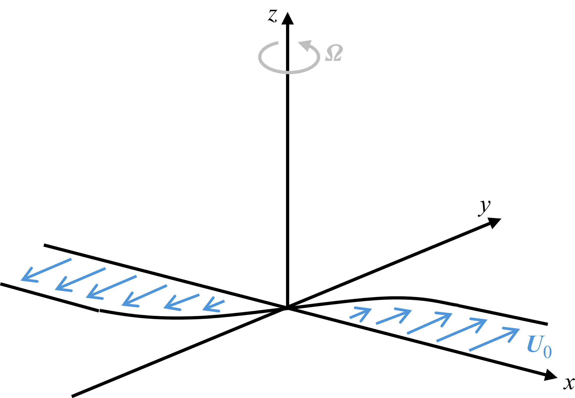


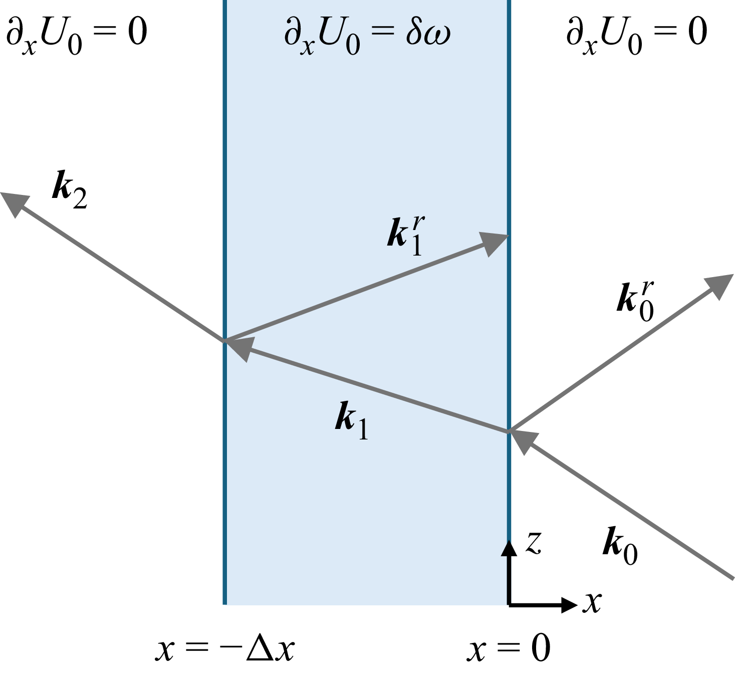

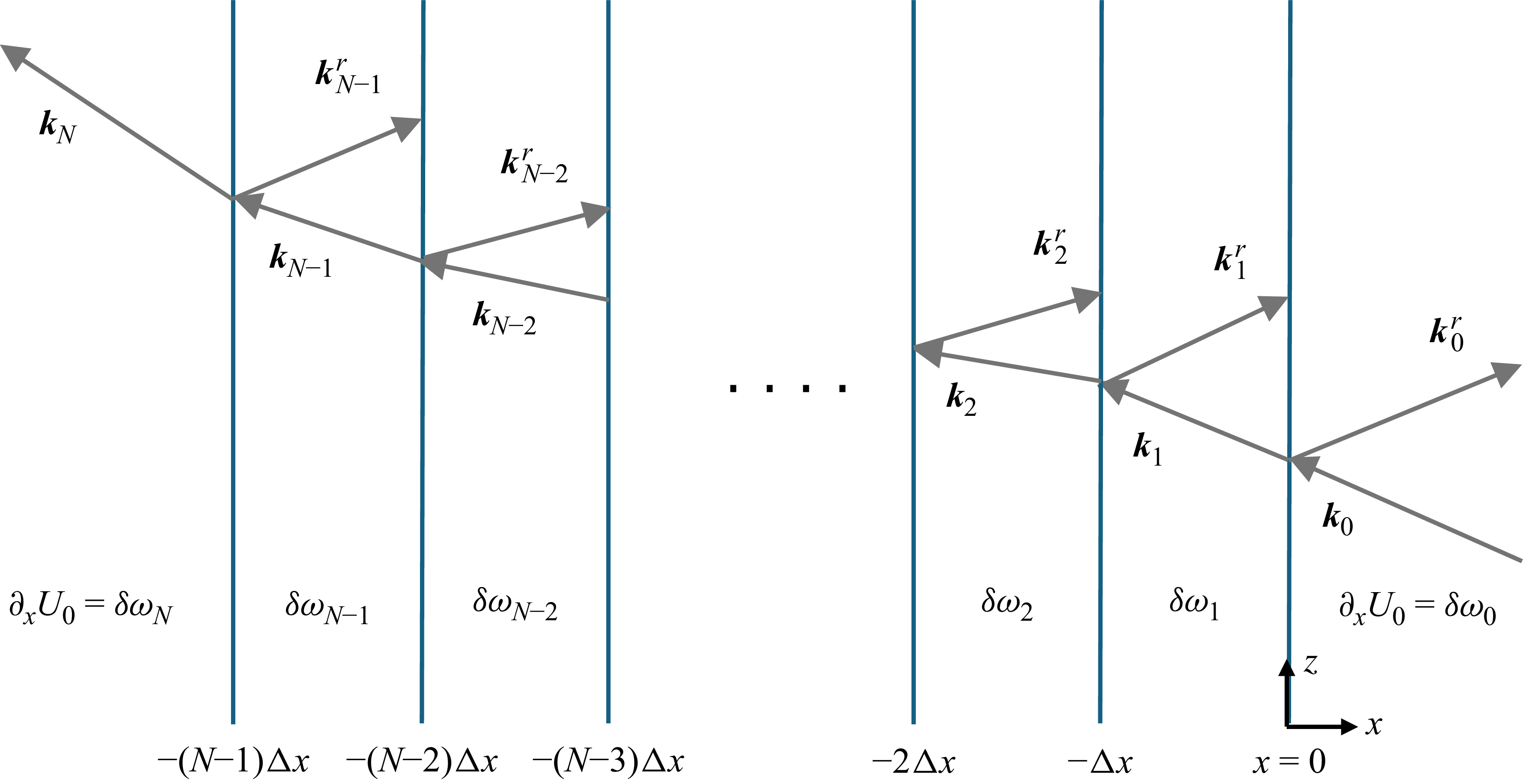

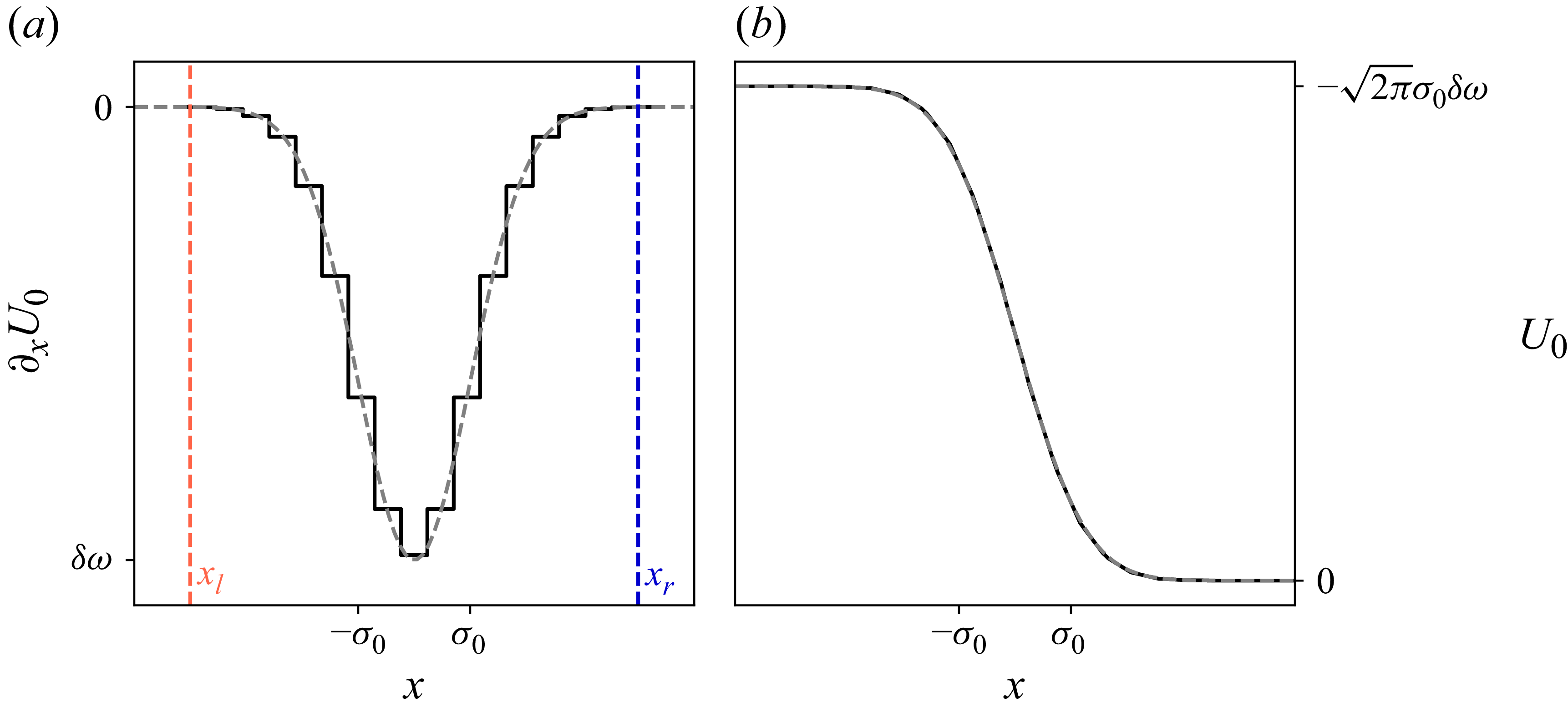


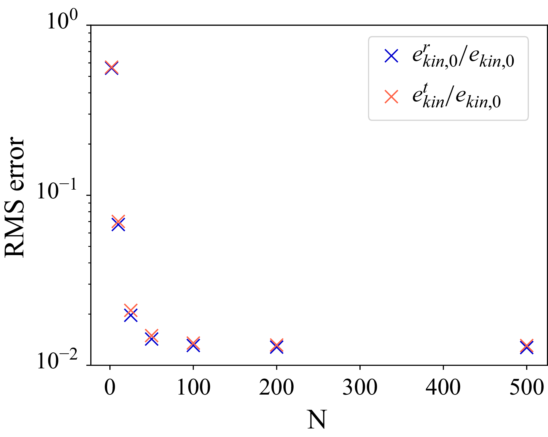


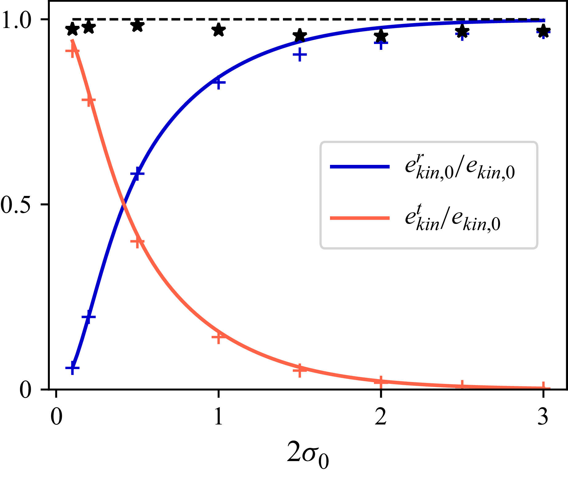
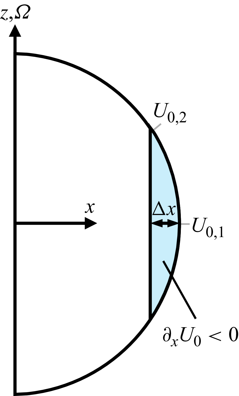

 Open access