


1. Introduction
This paper studies resonances and wave patterns in a circular channel with a submerged, symmetrical hill. Surface waves are forced by a periodic motion of a circular tank. In nature, periodic forcing can appear due to tidal motions stimulating nonlinear surface waves such as solitons and bores. Tidal bores, for example, can be found in rivers when the tide at the mouth of the river is rising above the river's surface level, see Chanson (Reference Chanson2009) and Chanson (Reference Chanson2010). In general, tidal flows over bottom topography is a process important in shallow parts of the ocean. From the total amount of tidal energy from the Sun and Moon ( $3.7$ TW), $2.6$ TW go into the shallow seas (Munk & Wunsch Reference Munk and Wunsch1998). It is also relevant in tidally influenced estuaries and the rivers or streams flowing into it. Localised and breaking surface waves lead to mixing. This can influence the surface transport of nutrients but also the dispersion of polluted water. Here we study ‘tide’ generated solitons and undular bores experimentally and use a 3-D-printed submerged obstacle as a wave maker.
Waves induced by stationary flows over single mountains are a well-studied subject. For example Houghton & Kasahara (Reference Houghton and Kasahara1968) used a hydrostatic shallow-water approach to derive analytical nonlinear solutions with hydraulic jumps. This was later generalised by Baines (Reference Baines1984) for two-layer flows. The results have been complemented by numerical solutions using different numerical methods in Nadiga, Margolin & Smolarkiewicz (Reference Nadiga, Margolin and Smolarkiewicz1996). Considering the problem of sliding underwater landscapes, the effect of a temporally changing topography located at the bottom of a fluid layer has been studied by Tinti & Bortolucci (Reference Tinti and Bortolucci2000). Bathymetry is not only for making waves: it is well-known that in a fluid at rest, wave scattering, reflection and transmission can be observed if waves pass over topographies. A detailed analytical discussion is made in Mei (Reference Mei1985). Mei, Hara & Naciri (Reference Mei, Hara and Naciri1988) studied the so-called Bragg scattering of water waves propagating over periodic bathymetries applying the Klein–Gordon equation. A detailed discussion of the dependence of the reflection coefficient on the wavenumber was held by Nayfeh & Hawwa (Reference Nayfeh and Hawwa1994). The reflection of waves by a doubly sinusoidal bed was discussed by Rey, Guazzelli & Mei (Reference Rey, Guazzelli and Mei1996) and a clear dependency on the wave frequency could be proven.
A submerged hill in a channel with periodic boundary conditions and with periodic forcing represents a generalisation of sloshing in a rectangular channel (Chester & Bones Reference Chester and Bones1968; Bouscasse et al. Reference Bouscasse, Colagrossi, Antuono and Lugni2013; Harlander et al. Reference Harlander, Schön, Borcia, Richter, Borcia and Bestehorn2024). In addition, it combines features of topographic overflow with the scattering of waves, since the periodic excitation of the flow at the obstacle generates not only stationary but also propagating waves, which in turn interact with the topography. The hill can thus be seen as a partially blocking barrier, which can reflect but also transmit waves and it is of interest to change the aspect ratio
 \begin{equation} \delta_{hill} = \frac{h_{hill}}{h_0}, \end{equation}
whereby  $h_0$ is the mean fluid depth away from the hill and $h_{hill}$ denotes the height of the hill. This height variation is relevant for investigating the range of resonances between complete blocking, i.e. a classic sloshing experiment, and the gradual transition to complete transmission at small $\delta _{hill}$. The linear investigation of the closed channel sloshing problem shows that a sloshing system has the fundamental eigenfrequency $\omega _0 = {\rm \pi}\sqrt {gh_0}/L$ (Faltinsen, Rognebakke & Timokha Reference Faltinsen, Rognebakke and Timokha2006), where $g$ is the constant of gravity and $L$ the channel length. For $\delta _{hill}$ of $ O (1)$ this eigenfrequency should also play a role for the submerged hill system, however, deviations can be expected when $\delta _{hill}$ becomes significantly smaller since then reflected waves can interact with waves passing the obstacle.
The oscillating circular channel is part of a wave tank at the Fluid Centre of the authors’ university mounted on a rotating platform. It was previously used for rotating convection experiments (Rodda et al. Reference Rodda, Hien, Achatz and Harlander2020) but later the outer heating chamber with its ideal circular shape was taken to investigate internal waves (Le Gal et al. Reference Le Gal, Harlander, Borcia, Le Dizès, Chen and Favier2021) and surface waves in circular channels (Borcia et al. Reference Borcia, Borcia, Xu, Bestehorn, Richter and Harlander2020). The latter investigated undular bores and their collision, produced by initial water level differences. In Borcia et al. (Reference Borcia, Richter, Borcia, Schön, Harlander and Bestehorn2023), sloshing with a fully blocking barrier was studied.
To accompany the experiments numerically we use a model derived by using the long-wave approximation by means with a Kármán–Pohlhausen approach (Bestehorn, Han & Oron Reference Bestehorn, Han and Oron2013). Because of the weak curvature of the channel  ${2{\rm \pi} d}/{L} = 0.11$, where $d$ is the channel width, the model geometry is considered to be rectangular, hence curvature effects were neglected at first order. Therefore, a two-dimensional (2-D) flow with velocity vector $\boldsymbol {v} = (u, w)^T$ is assumed. The incompressible Navier–Strokes equation for Newtonian fluids reads
 \begin{equation} \partial_t \boldsymbol{v} + (\boldsymbol{v} \boldsymbol{\cdot} \boldsymbol{\nabla}) \boldsymbol{v} = \nu\Delta\boldsymbol{v} - \boldsymbol{\nabla} p + \boldsymbol{f}_e, \end{equation}
where  $p$ denotes the pressure divided by the constant density, $\nu$ the kinematic viscosity and $\boldsymbol {f}_e= (b(t), -g)^T$ the external force. Here $b(t)$ is the periodic external forcing.
The velocity at mid-channel in the experiment is
 \begin{equation} v_{ex}(t) =A \sin(\omega t ). \end{equation}
Therefore, the horizontal term of external acceleration in (1.2) can be found with
 \begin{equation} b(t) = \partial_t v_{ex}(t) = A \omega \cos(\omega t). \end{equation}
The amplitude of velocity is  $A$ and the angular frequency is $\omega$. The characteristic aspect ratio of the system is
 \begin{equation} \delta = \frac{h_0}{L}. \end{equation}
The ratio of velocity amplitude to wave speed is expressed with the Froude number
 \begin{equation} Fr_{A} = \frac{A}{c_0}, \end{equation}
whereby  $c_0 = \sqrt {g h_0 }$ is the shallow-water wave speed. The conservation of mass is in that case expressed through incompressibility
 \begin{equation} \boldsymbol{\nabla} \boldsymbol{\cdot} \boldsymbol{ v} = 0, \end{equation}
and the bottom boundary condition is given by
 \begin{equation} \boldsymbol{v}=0, \quad \text{at} \ z = f(x). \end{equation}
Here,  $f(x)$ is the bottom topography. The topography used in the experiment is represented by the topographic function
 \begin{equation} f(x) = \frac{h_{hill}}{2}\left[1-\cos\left(\frac{2{\rm \pi} \left(x-\dfrac{L_{hill}}{2}\right)}{L_{hill}}\right)\right]\left[\varTheta\left(x+ \frac{L_{hill}}{2}\right)-\varTheta\left(x-\frac{L_{hill}}{2}\right) \right], \end{equation}
whereby  $\varTheta$ denotes the Heaviside function and $L_{hill}$ the mountain length. Equation (1.9) represents a stand-alone submerged mountain. Due to the periodic boundaries in the $x$ direction, the topography can more accurately be seen as a group of mountains having a distance $L$ from each other. Note that the chosen topographic function guarantees that $f$ is smooth at $\pm {L_{hill}}/{2}$, which increases the durability of the numerical calculation. On the surface of the fluid layer, the kinematic boundary condition is given by
 \begin{equation} \partial_t h = w - u \partial_x h. \end{equation}
Here  $h= h(x,t)$ denotes a stress-free deformable surface, where the stress-free assumption can be expressed by
 \begin{equation} p = p_0 - \boldsymbol{n}^T \boldsymbol{\cdot} 2\eta D \boldsymbol{\cdot} \boldsymbol{n}, \quad \text{at}\ z= h(x,t), \end{equation}
where  $p_0$, $\boldsymbol { n}$ and $D_{ij} = (\partial _i v_j + \partial _j v_i)/2$ denote environmental pressure, the surface normal vector and shear rate, respectively. Note that the numerical model described is an established model in the context of thin-film fluid mechanics heavily used for microfluids, e.g. lubrication problems and thin-liquid-film instabilities. With respect to the specific problems considered here, this has not been applied much. We show that the model is able to reproduce the resonance frequencies and the variety of patterns at the fluid surface observed experimentally. Moreover, the model is tested against the 2-D Navier–Stokes model by Borcia et al. (Reference Borcia, Richter, Borcia, Schön, Harlander and Bestehorn2023). Hence, with this simple long-wave model we can resolve the parameter space in greater detail compared with the rather elaborate experiments. This will be important in particular for future research on more theoretical aspects.
In the following, we show that changing the boundaries of a channel sloshing experiment from closed to periodic opens the possibility of studying wave topography interactions by installing a submerged hill. Such a hill can of course also be installed in a closed channel, but then the surface wave field would mainly be determined by the wave reflection at the end walls. A key point of the study is to generalise the resonance spectrum for a sloshing experiment allowing for wave transmission. By changing the fluid height we can cover Froude numbers that range from the case of a complete blockage to a flat topography where mainly transient lee wave effects play a role. The parameter range covers values ranging from locally subcritical to critical flow with strong nonlinearities. To the best of the authors’ knowledge, this has not yet been investigated experimentally in such detail for a sloshing experiment with periodic boundaries.
The main goal of the present study is to delineate surface wave patterns and resonances for different surface–hill ratios  $\delta _{hill}$. For this purpose, we investigate five cases in the following. Cases 1, 2 and 3 are in the transient region according to the stationary overflow problem. Cases 4 and 5 are in the non-transient subcritical region of the stationary topographic flow. Hereby, cases 3 and 4 lie near the marginal line separating subcritical from critical behaviour. Case 0 is data we took from Borcia et al. (Reference Borcia, Richter, Borcia, Schön, Harlander and Bestehorn2023), for the comparison with a case of complete blockage. All cases and their exact parameters are given in table 1.
Table 1. Measurement parameters. Case 0 was taken from Borcia et al. (Reference Borcia, Richter, Borcia, Schön, Harlander and Bestehorn2023). The excitation amplitude and the mountain height are kept constant for every measurement, with  $A = 0.159\, \mathrm {m}\,\mathrm {s}^{-1}$ and $h_{hill} = 2\,\mathrm {cm}$.

2. Methods
2.1. Experimental method
The experimental set-up is a circular tank made out of acrylic glass mounted on a rotating table. The used topography is a 3-D-printed hill with height  $h_{hill}=2 \, \mathrm {cm}$ and length $L_{hill} = 30\, \mathrm {cm}$. Its shape was adapted to the channel's curvature. The relative mountain height is denoted with $\delta _{hill} = h_{hill}/h_0$, where $h_0$ is the mean height of the water level. Surface height measurements are conducted by means of 17 ultrasonic probes. All 17 of these identical sensors can be placed at any distance from each other at a circular aluminium profile fixed above the circular channel (see figure 1). The channel width is $d = 8.5\,\mathrm {cm}$.

Figure 1. Experimental set-up, circular tank, with 17 ultrasonic probes mounted on the curved aluminium profile.
To measure wave propagation, it was decided to place the sensors equidistant over one-half of the channel's centreline with a total length of  $L = 476\,\mathrm {cm}$. For this, we introduced the $x$ coordinate in centimetres, related to the length of the centreline instead of using rad or degrees. Hereby, the first sensor is placed directly over the hill, which is declared to be $x = 0$ cm. The 17th sensor is at the opposite side of the channel at $x = 238.0\,\mathrm {cm}$. The remaining 15 sensors are placed in between these two sensors with a distance of $14.9\,\mathrm {cm}$. Due to the symmetry of the set-up, it is possible to reconstruct the wave structures in the whole channel by mirroring the sensor signals and positions. To control the symmetry, an additional 18th synch sensor is placed symmetrically to sensor 6 in the other half of the channel. The signals of sensors 6 and 18 should be shifted in phase by a factor ${\rm \pi}$. The position of the sensors is sketched in figure 2.

Figure 2. Schematic sketch of the experiment, with the mid-channel length  $L =4.76\,\mathrm {m}$ and gap width $d = 8.5\,\mathrm {cm}$.
The equidistant ultrasonic probes are mic +25 from microsonic GmbH, and the 18th sensor is from a P47 series of PIL Sensoren GmbH. Ultrasonic distance sensors usually work in three steps. First a pulsed sound wave is sent by a speaker with the constant sound velocity. Then the time delay  $\Delta t$ between emitted and received sound wave is measured by the sensor. Finally, the transit time of the signal is converted into a distance.
The sensors used in our experiments have an analogue output of 0–10 V. This output is connected to a data acquisition card, where the computer interprets the voltage as distance. The mic +25 sensors produce a cone of sound which is  $10\,\mathrm {mm}$ in diameter, at still water level. Note that the cone in this particular instrument is almost cylindrical.
The surface wave excitation is performed by the rotating table whose rotation oscillates with a given amplitude and frequency. During a measurement, the frequency increases in steps. For each frequency step, the system was given 2 min time, which was enough to reach a stable state. This steady state is reached after 3–5 oscillations.
2.2. Numerical method
Solving momentum equation (1.2) numerically can be computationally expensive. The geometric shape of the problem allows the use of the long-wave approximation according to Oron, Davis & Bankoff (Reference Oron, Davis and Bankoff1997). The long-wave approximation can be applied if the characteristic ratio fulfils the condition  $|\delta |\ll 1$. Here, $h_0$ is the medium depth and $L$ is the system length. The system coordinates can be scaled to this ratio as
 \begin{equation} x = \frac{h_0}{\delta}x^\prime, \quad z= h_0 z^\prime, \quad t = \frac{h_0}{\delta c_0}t^\prime. \end{equation}
Furthermore, we scale the quantities
 \begin{equation} \left. \begin{gathered} (h,f)= h_0 (h^\prime, f^\prime), \quad u = c_0 u^\prime,\quad w = c_0 \delta w^\prime ,\quad p=c_0 ^2 p^\prime, \quad A = c_0 Fr_A,\\ \omega = \frac{\delta c_0 }{h_0} \omega^ \prime,\quad b=\frac{ \delta c_0 ^2}{h_0} b', \end{gathered} \right\}\end{equation}
where the prime denotes dimensionless quantities. Now the dimensionless momentum equation can be expressed (dropping all primes) as
 \begin{equation} \delta \left[ \partial_t u + \left(u \partial_x+ w\partial_z\right)u\right] = \frac{\nu }{c_0h_0 } \nabla_\delta^2 u - \delta\partial_x p + \delta b \end{equation}
and
 \begin{equation} \delta^3\left[ \partial_t w + \left(u \partial_x + w\partial_z\right)w\right] =\frac{ \delta^2\nu}{c_0h_0} \nabla_\delta^2 w - \delta\partial_z p - \delta g. \end{equation}
Here  $\nabla ^2_\delta =\delta ^2 \partial ^2_x+\partial ^2_z$ and $b$ is an external excitation from (1.4). In the following, we neglect all terms of ${ O }(\delta ^2)$ or smaller. The $w$ term in (2.3) can be eliminated with the continuity equation. From (2.4) and stress-free condition (1.11), a solution of the (dimensionless) hydrostatic pressure equation is
 \begin{equation} p ={-} \frac{ h_0}{c_0^2}g z + \frac{ h_0}{c_0^2} g h. \end{equation}
Inserting (2.5) in (2.3), gives the long-wave equation
 \begin{equation} \partial_t u + \left(u \partial_x + w\partial_z\right)u = \frac{1}{{\textit{Re}}}\partial_{zz} u - \partial_x h + b. \end{equation}
 The ratio between wave velocity, system size and viscosity is expressed by the Reynolds number  ${\textit {Re}} = {c_0h_0 \delta }/{\nu }$, which, for consistency, should be ${ O } (1)$. This is true in the Stokes boundary layer that scales with $1/\beta =(2 \nu /\omega )^{1/2}$, however, ${\textit {Re}}$ is larger outside this layer. Here we still keep the small viscous term ${{\textit {Re}}}^{-1} \partial _{zz} u$ because it stabilises the numerical calculations. The results are not altered much by the small term. To further increase the numerical performance of the model we separate the $z$ coordinate by assuming $u = q(x,t) g(z)$. Here $g(z)$ needs to fulfil the boundary condition (1.8). The flow rate is defined as
 \begin{equation} q(x,t) = \int_{f(x)}^{h(x,t)} u \,{\rm d}z, \quad \text{implying} \ \int_{f(x)}^{h(x,t)} g(z) \,{\rm d}z = 1. \end{equation}
This is called the Kármán–Pohlhausen approach by Craster & Matar (Reference Craster and Matar2009). This method was also used by Schön & Bestehorn (Reference Schön and Bestehorn2023) and Bestehorn et al. (Reference Bestehorn, Han and Oron2013). A sketch of the connection between  $u$ and $q$ is shown in figure 3. Here, for $g(z)$ a boundary layer profile is chosen:
 \begin{equation} g(z; x,t) = \frac{K}{H} \left(1 - \frac{\cosh{\tilde{\beta}(h-z)} }{\cosh{\tilde{\beta} H}}\right), \end{equation}
with the factor
 \begin{equation} K (x,t)= \left(1- \frac{\tanh\left(\tilde{\beta} H\right)}{\tilde{\beta} H}\right)^{{-}1}. \end{equation}
The size of the boundary layer is the non-dimensional Stokes depth  $1/\tilde {\beta }=1/(\beta h_0)$. The fluid layer thickness is denoted by $H(x,t) = h(x,t)-f(x)$. Integration of (2.6) over $z$ (see Appendix A) leads to the equation
 \begin{equation} \partial_t q = H\left(-\frac{K\tilde{\beta} \tanh{\tilde{\beta} H }}{{\textit{Re}}}\frac{ q}{H^2} - \partial_x h + b\right)-\frac{2K q\partial_x q }{ H} +\frac{Kq^{2}}{ H^{2}} \partial_x H. \end{equation}
Here we assume that the parameters  $K(x,t)\approx 1$ in the relevant range $5 \le \tilde {\beta } H \le 60$. Note that it is also possible to choose a parabola or a linear shape for $g(z)$. The kind of profile will only change the prefactors of convection, diffusion and viscous damping terms. Note, further, that by skipping the viscous term ${{\textit {Re}}}^{-1} \partial _{zz} u$ in (2.6), the (2.10) and (2.11) would turn into the shallow-water equations with $g(z)=1$, $u=q/H$ and $\partial _z u |_{z=f}=0$. Here, the boundary layer profile (2.8) was chosen after the evaluation of the experimental flow profile by particle image velocity measurements. These measurements have been published in Borcia et al. (Reference Borcia, Bestehorn, Borcia, Schön, Harlander and Richter2024).

Figure 3. Assuming that the horizontal velocity  $u$ has a hyperbolic shape with respect to $z$, the flow rate $q$ is an integral of $u$ over $z$, covering the region from the bottom topography $f(x)$ to the liquid surface $h(x,t)$.
Equation (2.10) can be solved with the help of kinematic boundary condition (1.10) which after integration turns into
 \begin{equation} \partial_t h ={-} \partial_x q. \end{equation}
Equations (2.10) and (2.11) describe the system of a 2-D channel with a free surface of temporal changing force. It can be applied to a variety of different cases, just by choosing different  $f(x)$ and $b(t)$. Hereby, the long-wave character of the system under consideration ( $|\delta | < 1$ ) must be guaranteed. It should be noted that numerical instability can appear if $H$ gets too small. This is the reason why the numerical results we present here show small $h_{hill}/ h_0$ ratios.
We apply two modifications to enhance the stability of the numerical model. First, we use a logarithmic transform similar to Schmidt (Reference Schmidt1990) and Harlander (Reference Harlander1997), i.e. solving
 \begin{equation} \partial_{t} \tilde{p} ={-}\frac{\partial_x q}{H}, \end{equation}
where  $\tilde {p} = \ln (H)$, instead of (2.11). This method avoids negative or zero values of $H$. Second, we use a damping term related to the disjoining pressure, namely $- ({\tilde {A}}/{H^3})$ in (1.11), see Bestehorn & Borcia (Reference Bestehorn and Borcia2010). This term causes strong damping of flow rates that diverge for too low values of $H$ near the hill. However, this method should be applied with caution, because in contrast to (2.12) it can change the physics of the equation fundamentally if $\tilde {A}$ is chosen too high. We only applied the second method to case 3, and chose $\tilde {A} = 0.012$.
3. Results and discussion
In this section, we discuss the main results and compare the findings from the experiment and the numerical simulation. We start with a discussion on the amplitude spectra and subsequently, we consider the surface wave patterns at the different resonance peaks.
3.1. Amplitude spectra
We assume that a wave propagates with the shallow-water wave speed  $c_0=\pm (g h)^{1/2}$. At $t_1$ we accept that it starts to propagate when the excitation function is at an extreme value, with phase $\omega t_1$. Then it travels from one side of the mountain, through the channel, to its opposite side. The wave will reach its starting position at $t_2 = t_1 + L/c_0$. At this time, the phase of the excitation is $\omega (t_1+ L/c_0)$. The excitation will have an extremum at $t_2$, if
 \begin{equation} \omega = n \frac{{\rm \pi} c_0 }{L}= n\omega_0. \end{equation}
Hereby, we denote the first eigenfrequency by  $\omega _0$. The direction of the hill motion is opposite to the wave motion if $n$ is odd. If $n$ is even, the wave and hill motion will be in the same direction. It can be concluded that even eigenfrequencies produce a constructive resonance if the wave is able to cross the mountain. Odd eigenfrequencies produce constructive resonance if the wave is reflected from the mountain. The reflecting resonance at odd eigenfrequencies was shown for the total blocking case in several papers (Faltinsen et al. Reference Faltinsen, Rognebakke and Timokha2006; Bouscasse et al. Reference Bouscasse, Colagrossi, Antuono and Lugni2013; Bäuerlein & Avila Reference Bäuerlein and Avila2021; Borcia et al. Reference Borcia, Richter, Borcia, Schön, Harlander and Bestehorn2023, e.g.).
The potential energy of the wave field at a certain time is given by
 \begin{equation} E_{pot}(t) = \frac{1}{2}\int_{{-}L/2}^{L/2} g d \rho h^2(x,t) \,{{\rm d}\kern0.07em x}. \end{equation}
see Tinti & Bortolucci (Reference Tinti and Bortolucci2000). We see that the energy of the wave field depends on the square of the wave amplitude  $h$. To discuss the wave excitation at different excitation frequencies $\omega$, a local potential energy density ( ${J/m}$) is calculated as follows
 \begin{equation} \frac{g h_0 \rho}{2} \langle h^2 (x) \rangle = \frac{g h_0 \rho}{2T} \int_{t}^{t+T} h^2(x,t) \,{\rm d}t = \frac{g h_0 \rho}{2T} \int_{t}^{t+T} (\Delta h(x,t))^2 \,{\rm d}t + e_0. \end{equation}
Here, the relative surface displacement  $\Delta h (x,t)= h(x,t) - h_0$. Variations of $\langle h^2(x) \rangle$ over frequency can be understood as an amplitude spectrum. For convenience, we choose the constant offset local energy $e_0 = 0$.
The envelope of the amplitude spectra for the cases listed in table 1 is plotted in figure 4. Case 0 is a fully blocking case ( $\delta _{hill} \gg 1$). It shows exclusively constructive resonance at odd eigenfrequencies. In contrast, case 1 ( $\delta _{hill} = 1$) shows minor peaks at odd $n$ and no peaks at even eigenfrequencies. This is a partial blocking case, whereby the excited waves are able to spill over the mountain. At all frequencies, $\langle h^2 \rangle$ is rather large. Case 2 has an almost flat spectrum. This means that waves with high amplitudes are excited independent of the frequency, i.e. resonance plays no prominent role for the excitation of surface waves. As can be seen from figure 5, cases 1 and 2 are located in the critical region of the stationary flow regime. This means that local effects, i.e. the motion of the fluid over the topography only, are already sufficient for a significant transfer of energy from the flow to surface waves. So far, the only distinct peaks appear in cases 0 and 1 for odd $n$, showing that wave focusing due to resonant wave reflection is the dominant process. A further decrease of $\delta _{hill}$, however, gives rise to new peaks. For case 3, regions of higher amplitudes appear close to even but also, with smaller amplitudes, to odd eigenfrequencies. This case is still in the critical regime as visible in figure 5, but the appearance of odd and even peaks in the spectrum suggests that reflective and transitive resonating waves have been excited. In case 4, peaks become more prominent. This case is in the subcritical part of the regime (see figure 5), which means the Froude number is not large enough for a wave excitation due to a pure non-resonant motion of the fluid. Note that even peaks are the largest and that, compared with case 3, the ratio of odd peak height to even peak height has decreased. The localisation of even peaks is further enhanced in case 5 but the peak amplitudes become somewhat smaller. An increase of reflection at topographies, due to an increase in topography height was found by Mei (Reference Mei1985), Mei et al. (Reference Mei, Hara and Naciri1988), Nayfeh & Hawwa (Reference Nayfeh and Hawwa1994) and Rey et al. (Reference Rey, Guazzelli and Mei1996). This confirms the observation of shrinking reflection peaks with increasing $\delta _{hill}$.

Figure 4. Amplitude spectrum for different cases (see table 1 and figure 5), solid black line is the envelope of  $\langle h^2 \rangle$ from the experiment. The dashed line is the envelope of the numeric solution. Every dot is the measurement of a Sensor, the colour represents its distance from the barrier. The dotted line in case 0 is the full Navier–Strokes solution from Borcia et al. (Reference Borcia, Richter, Borcia, Schön, Harlander and Bestehorn2023).

Figure 5. Regime diagram, reproduced from Houghton & Kasahara (Reference Houghton and Kasahara1968). The cases from table 1 are plotted according to their excitation amplitude. Note that subcritical (supercritical), denotes a constant flow velocity  $u_0$ lower (higher) than the surface wave phase velocity $c_0$.
Borcia et al. (Reference Borcia, Richter, Borcia, Schön, Harlander and Bestehorn2023) observed that the odd peaks in case 0 decrease in height with increasing frequency by a factor  $1/\omega$. This factor can be traced back to the amplitude of the oscillating barrier displacement. Because of the comparably small excitation amplitudes for fully blocked cases, Borcia et al. (Reference Borcia, Richter, Borcia, Schön, Harlander and Bestehorn2023) were able to investigate the spectra up to the 7th eigenfrequency. In the present study, the same engine and gearbox are used in the experiment, but with approximately 10 times higher amplitudes (see table 1). This severely limits the maximum frequency we can apply without damaging the experimental apparatus.
The numerical solution of cases 3–5 shows slightly higher envelopes (dashed lines in figure 4) for lower frequencies and lower ones for higher frequencies. This effect intensifies with increasing  $\delta _{hill}$. The reason could be a shortcoming of the long-wave approximation since higher excitation frequencies cause more shortwave structures not represented by the model assumptions. Moreover, the peaks of the numerically calculated resonances are slightly shifted towards larger frequencies compared with the experimental data. It should be mentioned that the dotted line in case 0 of figure 4 is the solution taken from a different numerical model and was reproduced here from Borcia et al. (Reference Borcia, Richter, Borcia, Schön, Harlander and Bestehorn2023). The dashed line is (2.10) and (2.11) calculated by applying fixed boundaries and $f(x) =0$.
3.2. Wave patterns
Inside the rather broad region of a resonance peak, a wide variety of patterns can be observed. Therefore, it is important to first clarify the used designation of the different wave types. We call a wave-train with multiple peaks propagating in the same direction with the same speed an undular bore. A high-amplitude single propagating wave is coined a soliton, a travelling dent in the surface an antisoliton and a wide low-intensity wave a cnodial wave. The latter three are inspired by eponymous solutions of the Korteweg–de Vries equation. To discuss these wave patterns in an efficient way, we use space–time plots where the wave field is plotted over the whole channel ( $x/L$ axis) and two periods of excitation ( $t/T$ axis). In figure 6, it is shown how a single wave reflected at a fixed barrier (case 0) is represented in such a space–time plot. The localised crest (red colour) propagates back and forth between the barrier located at $x/L=\pm 0.5$. It is obvious that the wave amplitude is largest at the barrier and becomes smaller during propagation until it reaches the opposite side of the barrier where the wave is reinforced again by the moving barrier. Next, to explain reflection and transmission at the topography we exemplary display two space–time diagrams taken from case 2, because in this case, the waves have rather similar heights for the chosen forcing frequencies. An example of an almost full wave reflection at the hill at $x/L=0$ is shown in figure 7. It can be observed that an incident wave at the mountain splits into two parts. A small part of the wave energy can pass the hill but the main part is reflected. Clearly, this diagram looks rather similar to figure 6 when the position of the hill is mapped to the barrier position $x/L=\pm 0.5$. Essentially, the wave energy is reflected back and forth between the hills as for the situation displayed for the barrier. A very different picture emerges when we consider the same $\delta _{hill}$ but force the flow by approximately twice the frequency (see figure 8). Now we find a weak reflection and a prominent wave transmission. The reflected part manifests itself in fine lines, however, those fine structures are in fact difficult to recognise in the figure due to its very low amplitude.

Figure 6. A reflected wave calculated with the long-wave model with parameters from case 0. Fixed boundary is located at  $x/L= \pm 0.5$.

Figure 7. A reflected wave patten from case 2 (experiment). Bathymetry is located at  $x/L=0$.

Figure 8. A transmitted wave pattern from case 2 (experiment). Bathymetry is located at  $x/L=0$.
Equipped with this basic understanding of wave reflection and transmission in a space–time representation we are now in a position to discuss the variety of wave patterns that occur for forcing frequencies in a range that covers four resonance peaks. We focus here on case 4 since it is representative for cases where wave transmission becomes more and more important for decreasing  $\delta _{hill}$. Moreover, case 4 is very suitable for our purpose since for this case we have experimental and numerical data. Comparing case 4 to cases 2, 3 and 5, the main differences concern, as mentioned before, amplitude and amplitude ratio, and not so much the qualitative appearance of the wave patterns.
Near the first eigenfrequency (figure 9  $\omega /\omega _0 = 0.940$) undular bores are observed that show reflecting behaviour. Every half-period (i.e. $t/T=1/2$, 1, $3/2$ and $2$) a reflection happens where the place of reflection changes each time from one side of the mountain to the other. A small part of the wave energy is transmitted over the hill. An increase of frequency to $\omega /\omega _0 = 0.966$ leads to a reduction of undulations in the bores.

Figure 9. Space–time plots in an oscillatory frame of reference for different frequencies, for case 4. Long-wave model and experimental results are shown. The topography is placed at  $x=0$. The colourmap is given in $\Delta h/ h_0$. Time is normed to the last two periods measured before the frequency change.
With a frequency near the second amplitude peak ( $\omega /\omega _0 = 1.670$), it can be observed that two wave structures propagate in opposite directions through the channel. In the lower-frequency to the higher-frequency part of the peak, undular bores (figure 9, ${\omega /\omega _0=1.905}$), solitons (figure 9, $\omega /\omega _0=2.062$) and cnodial waves (figure 9, $\omega /\omega _0=2.349$) are observed. The undular bore type covers the largest part of the spectrum. Hereby, it should be mentioned that the number of undulations decreases with increasing frequency. Solitons occur almost exactly at the second eigenfrequency. Cnodial waves show no transmissive but reflecting behaviour only.
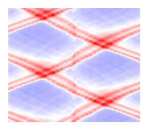
At the third eigenfrequency ( $\omega /\omega _0 = 3.001$) a quite regular quasi-square-shaped pattern is observed. This pattern seems to result from collisions of a number of waves. It is hard to say whether wave reflection is involved, expected for odd values of $\omega /\omega _0$, or if a process is involved at which waves are amplified not every, but every second oscillation. Likely we see a superimposition of both effects.
The fourth natural frequency shows four wave structures, two propagating to the left and two propagating to the right with similar structures. Crossing the resonance peak, the change of wave types is qualitatively similar to what we already found for the second peak. We see an undular bore with four crests at  $\omega /\omega _0 =3.706$, and four solitons at a slightly higher frequency, $\omega /\omega _0 = 4.071$. In between the peaks in the amplitude spectrum, wave structures can be observed reminiscent of antisolitons (see figure 9, $\omega /\omega _0 = 1.67$ and $3.41$).
Near  $x =0$, waves that are able to cross the mountain show a crinkle in their trajectory. This crinkle is caused by a change in wave velocity under the influence of the bottom topography as can be expected by linear theory for which the phase velocity is $\sqrt {g(h_0 - f(x))}$. This implies that in the region close to $x \approx 0$, the wave speed shows a minimum. Physical intuition suggests a splitting of the waves in a transmitting and a reflecting part in regions with such a rather abrupt phase speed change. Note, finally, that the envelope of simulation and experiment displayed in figure 4 shows a rather perfect agreement between the second and fourth peaks of the amplitude spectrum. For lower frequencies, the simulation shows larger amplitudes than the experiment. This is caused by the formation of subcritical lee waves typical for stationary solutions. In the experiment, we placed only one sensor above the mountain, which hampers a clear understanding of the process. The lee wave in the simulation can be also seen in figure 9, at $x= 0$.
In summary, the long-wave model produces rather similar patterns compared to the experiment and is hence a useful and numerically cheap tool to supplement the experimental data. As expected, fine structures, visible especially for the undular bores (see, e.g., the case  $\omega /\omega _0=1.905$ in figure 9), do not appear in the simulation due to the long-wave approximation. Moreover, some of the patterns shown in figure 9 are also very sensitive to frequency. That is, patterns do not look very similar for the same excitation frequency but slight changes in frequency lead to a much better match between the space–time patterns. This is demonstrated for the frequencies $\omega /\omega _0=0.966$ and $2.010$. For the first frequency, we find a sign reversal in figure 9, for the second we see a much stronger localisation in the experiment compared with the simulation. Figure 10 exhibits the effect of a slight frequency change for these two examples and the frequency sensitivity is quite obvious. For frequencies especially near the resonance peaks, the patterns observed in the experiment appear at somewhat lower frequencies than in the numerical simulations.

Figure 10. Space–time plot comparison for similar patterns in experimental and numerical results. Two frequencies are chosen near the first and second eigenfrequency. The patterns appear in the experiment (a,c) at lower frequencies than in the numerical simulations (b,d).
4. Conclusion
In a circular channel, surface waves have been excited by means of a submerged hill that, together with the tank, performs a harmonic oscillation. The study is in the realm between channel sloshing, wave generation by stationary flows over mountains and wave scattering from submerged obstacles. A key point of the study was to experimentally derive the resonance spectrum for a sloshing experiment allowing for wave transmission. Froude numbers have been considered in a range from stationary subcritical to transient subcritical. To the best of the authors’ knowledge, this has not yet been investigated experimentally in such detail for a sloshing experiment with periodic boundaries.
It has been shown that the resonant frequencies of waves excited at the oscillating submerged hill depend on the aspect ratio  $\delta _{hill}$. For $\delta _{hill} \approx { O }(1)$ we recovered a resonance spectrum that resembles strongly that of the fully blocked sloshing case 0, for which just odd normalised frequencies occur since only modes corresponding to such frequencies resonate constructively. We called this resonance due to reflective amplification. For smaller $\delta _{hill}$ waves that pass the topography can also become resonant. Through a step-wise reduction of $\delta _{hill}$ we approached a resonance spectrum where the even frequencies dominate since now we find resonance due to transmissive amplification, i.e. here the modes passing the hill resonate constructively. In other words, we find even and odd multiples of the channel eigenfrequency depending on the direction of the hill's motion when an incoming wave encounters the hill: for reflection, the incoming wave and the hill's motion have opposite directions (odd frequency peaks); for transmission, the incoming wave and the hill's motion have the same direction (even frequency peaks). Obviously, transmissive resonance becomes more prominent for lower $\delta _{hill}$. Cases that are located in the critical stationary regime (see figure 5) show less-sharp peaks, but flatter amplitude spectra. It is remarkable that frequencies prohibited from the spectrum of the closed channel (destructive resonance for even frequencies) give rise to the largest amplification in the periodic case due to topographic fluid–structure interaction. Note that the oscillating flow over a submerged hill produces wave structures at Froude numbers where only subcritical waves are expected from the stationary flow problem.
In the second part of the study, we focused on the nonlinear wave structures excited by the oscillating topography in a periodic channel. We have found that the wave patterns depend strongly on the excitation frequency. Approaching the first resonance peak from the low-frequency side we observed antisolitons. With an increase of the excitation frequency, we found a wide frequency band in which undular bores are the most common structures. Hereby, their number of undulations can be reduced by increasing the frequency. By reaching the eigenfrequency deduced from linear theory, the train of waves collapsed into a single soliton. A further increase led to an abrupt reduction of wave amplitude and cnoidal waves were showing up. Note that at a multiple of an eigenfrequency, we observed a multiple of the wave structures described for the first peak.
Finally, we tested whether the resonances as well as the dominant wave structures can be reproduced by a highly simplified nonlinear 2-D long-wave shallow-water model. Very satisfactorily the model was able to qualitatively replicate the course structures of the wave patterns, their amplitudes and the amplitude spectrum. This opens the possibility for a subsequent more-theoretical study on wave resonance in a periodic channel by relying more on the fast numerical model.
Future research will address symmetry breaking due to asymmetric topography with symmetric forcing but also the reverse case, symmetric topography with asymmetric oscillatory excitation. For cases with symmetry breaking, we expect the development of a mean flow. Another focus will be on oscillating stratified flows over submerged hills that apply more to tidally forced oceanic flows.
Acknowledgement
We would like to thank the reviewer whose many critical comments helped to improve the manuscript significantly. F.T.S. thanks Matthias Strangfeld for fruitful scientific discussions. The authors further thank the technicians of the Department of Aerodynamics and Fluid Mechanics at BTU, Robin Stöbel and Stefan Rohark, for help with the experimental set-up and the technical equipment.
Funding
We acknowledge financial support from the German Research Foundation (grant numbers DFG BE 1300/25-1 and DFG HA 2932/17-4).
Declaration of interests
The authors report no conflict of interest.
Appendix A. Integrals
First, we reformulate
 \begin{equation} \left(u\partial_x+w\partial_z\right)u = \partial_x u^2 + \partial_z (uw). \end{equation}
This is possible because of incompressibility (1.7) through which we can replace
 \begin{equation} \partial_x u ={-} \partial_z w. \end{equation}
Thus, the following has to be solved:
 \begin{align} &\int_{f}^{h}\,{\rm d}z \,\partial_t u + \int_{f}^{h}\,{\rm d}z\, \partial_{x} u^2 + \int_{f}^{h}\,{\rm d}z\, \partial_z (wu)\nonumber\\ &\qquad = \int_{f}^{h}\,{\rm d}z \left(\frac{\nu }{c_0 h_0 \delta }\partial_{zz} u - \partial_x h +b(t)\right). \end{align}
With the Leibniz integration rule and all boundary conditions we obtain
 \begin{gather} \int_{f}^{h}\,{\rm d}z\,\partial_t u = \partial_t\int_{f}^{h}\,{\rm d}z\, u - \left.u\right|_h \partial_t h, \end{gather}
 \begin{gather} \int_{f}^{h}\,{\rm d}z\, \partial_{x} u^2 = \partial_{x}\int_{f}^{h}\,{\rm d}z\, u^2 - \left.u \right|_h^2 \partial_x h + \left.u \right|_f ^2 \partial_x\, f, \end{gather}
 \begin{gather} \int_{f}^{h}\,{\rm d}z\,\partial_z (wu) = \left[wu\right]^h_f=\left.u \right|_h \partial_t h + \left.u \right|_h^2 \partial_x h - \left.u \right|_f ^2 \partial_x\, f. \end{gather}
Adding (A4), (A5) and (A6), only the first term on the right-hand side of (A4) and the first term on the right-hand side of (A5) remain. Further,
 \begin{equation} \int_{f}^{h}\,{\rm d}z \left(\frac{\nu }{c_0 h_0\delta }\partial_{zz} u + \partial_x h + b \right) ={-}\frac{\nu }{c_0 h_0 \delta }\left.\partial_z u\right|_{z=f} + H\left[ -\partial_x h + b\right]. \end{equation}
Using the  $g(z)$ we introduced in the main text, it shows that $\partial _z u|_{z=f} = K\tilde {\beta } \tanh {(\tilde {\beta } H) }({q}/{H})$. The term $\partial _x\int _f ^h \,\textrm {d}z\, u^2 = \partial _x(K({q^2}/{H}))$. This gives the last two terms in (2.10).


 Open access