





1. Introduction
Slow flows around small bodies provide fundamental insights into micro- and nanofluidics, optofluidics, and aerosol engineering. Classical Stokes-flow solutions remain valuable for deepening our understanding of active microswimmers and for developing new applications (Daddi-Moussa-Ider et al. Reference Daddi-Moussa-Ider, Lisicki, Löwen and Menzel2020; Abdi & Nejat Pishkenari Reference Abdi and Nejat Pishkenari2021; Piro et al. Reference Piro, Vilfan, Golestanian and Mahault2024). As the size of the suspended body decreases, non-equilibrium flow phenomena (or non-Navier–Stokes effects) become increasingly important. Typical examples in gaseous media include thermophoresis (Takata & Sone Reference Takata and Sone1995; Takata Reference Takata2009; Bosworth et al. Reference Bosworth, Ventura, Ketsdever and Gimelshein2016; Kalempa & Sharipov Reference Kalempa and Sharipov2020) and the motion of Janus particles (Baier et al. Reference Baier, Tiwari, Shrestha, Klar and Hardt2018; Nosenko et al. Reference Nosenko, Luoni, Kaouk, Rubin-Zuzic and Thomas2020). In such cases, the mean free path of gas molecules becomes comparable to the characteristic size of the object and the gas is regarded as being rarefied. While rarefied gas flows around spherical bodies have been thoroughly investigated across a broad range of Knudsen numbers (see, e.g. Loyalka Reference Loyalka1992; Takata, Sone & Aoki Reference Takata, Sone and Aoki1993; Taguchi & Suzuki Reference Taguchi and Suzuki2017; Kalempa & Sharipov Reference Kalempa and Sharipov2020), systematic studies for non-spherical geometries remain limited. Here, the Knudsen number is defined as the ratio of the molecular mean free path to a characteristic length scale, such as the sphere radius. The case of spheroidal particles has been studied by Aoki, Takata & Tomota (Reference Aoki, Takata and Tomota2014), Livi et al. (Reference Livi, Di Staso, Clercx and Toschi2022), Clercx et al. (Reference Clercx, Livi, Di Staso and Toschi2024) and Zhang et al. (Reference Zhang, Chang, Wang and Xia2025). In this study, we consider the rarefied gas flow past a circular disk of infinitesimal thickness. Despite its geometric simplicity, the edge configuration introduces a distinctive flow feature absent in smooth geometries and its analysis is substantially more complex than that of a sphere, as described later.
Owing to its geometric simplicity, the rarefied gas flow around a circular disk is often regarded as a classical example of axisymmetric flow. Analytical expressions for the force acting on the disk have been derived in both the free-molecular flow limit (Dahneke Reference Dahneke1973; Ivanov & Yanshin Reference Ivanov and Yanshin1980, see also references therein) and in the near-free-molecular regime (Sengers et al. Reference Sengers, Lin Wang, Kamgar-Parsi and Dorfman2014). Numerical investigations have also been carried out in the high-speed flow regime (Shakhov Reference Shakhov1974; Chpoun et al. Reference Chpoun, Elizarova, Graur and Lengrand2005). A simple plate geometry (with or without thickness) has also been used as a model to study the unsteady decay of a moving body in a free-molecular gas (Aoki et al. Reference Aoki, Cavallaro, Marchioro and Pulvirenti2008; Aoki, Tsuji & Cavallaro Reference Aoki, Tsuji and Cavallaro2009). However, most existing studies have focused on drag evaluation or high-speed flow behaviour, and detailed investigations of the flow field structure in the low-speed regime, which is relevant to micro- and nanoscale applications, remain limited. In this context, the aim of the present study is twofold.
First, we aim to investigate the flow structure in the vicinity of the disk edge, where spatial variations in the flow variables occur on the scale of the molecular mean free path. Such edge effects have been studied primarily in the context of thermally induced flows (Aoki et al. Reference Aoki, Sone and Masukawa1995; Sone & Yoshimoto Reference Sone and Yoshimoto1997; Ketsdever et al. Reference Ketsdever, Gimelshein, Gimelshein and Selden2012; Taguchi & Aoki Reference Taguchi and Aoki2012) and their applications (e.g. Taguchi & Aoki Reference Taguchi and Aoki2015; Baier et al. Reference Baier, Hardt, Shahabi and Roohi2017; Lotfian & Roohi Reference Lotfian and Roohi2019; Wang et al. Reference Wang, Su, Zhang, Zhang and Zhang2020; Taguchi & Tsuji Reference Taguchi and Tsuji2022). However, much less is known about edge-induced effects in externally driven flows, despite their importance for understanding the behaviour of particles in motion within a gas. In particular, we focus on the formation of a localised kinetic boundary layer, referred to as the edge layer, which is distinct from the conventional Knudsen layer (Sone Reference Sone2007) that forms over smooth surfaces.
The second objective of the present study is to demonstrate the feasibility of numerically analysing a three-dimensional flow while accurately capturing discontinuities in the velocity distribution function (VDF). In the current problem, such discontinuities arise at the disk edge and propagate into the gas, and their precise representation is essential for correctly describing the flow field. One approach used in previous studies is a hybrid method that combines the finite-difference method with the method of characteristics. This method, originally introduced by Sugimoto & Sone (Reference Sugimoto and Sone1992) and applied to two-dimensional thermal edge flows by Taguchi & Aoki (Reference Taguchi and Aoki2012), offers both accuracy and computational efficiency. However, its implementation becomes increasingly difficult as the number of independent variables increases, making it impractical for the present three-dimensional setting. An alternative approach involves solving integral equations for macroscopic variables (see Chap. A.4.2 of Sone Reference Sone2007). This method accurately handles VDF discontinuities and is memory-efficient. It has been successfully applied to rarefied flows in rectangular cavities (Varoutis, Valougeorgis & Sharipov Reference Varoutis, Valougeorgis and Sharipov2008; Hattori Reference Hattori2024), where discontinuities arise at cavity corners. However, its implementation becomes considerably more involved in non-convex domains, since the integration domain, defined as the visible region from a given point, varies spatially and requires extensive problem-specific treatment. See, for example, its application to flows between non-coaxial cylinders (Aoki, Sone & Yano Reference Aoki, Sone and Yano1989) or through cylinder arrays (Taguchi & Charrier Reference Taguchi and Charrier2008).
In this study, we adopt a more direct strategy by integrating the original equation along its characteristics. Since the VDF itself is treated as the unknown, this method requires more numerical integration. Nevertheless, the associated computational cost can be alleviated through the use of high-performance computing. The present method is motivated by Taguchi, Tsuji & Kotera (Reference Taguchi, Tsuji and Kotera2021) (see also Tsuji & Aoki Reference Tsuji and Aoki2013), where an unsteady rarefied gas flow involving a discontinuous velocity distribution function was analysed by solving integral equations formulated for the VDF. We consider this approach a viable alternative to the finite-difference method for studying rarefied gas flows in complex geometries.
The remaining part of the paper is structured as follows. In § 2, we present the problem, providing its mathematical formulation based on the Bhatnagar–Gross–Krook (BGK) model (Bhatnagar, Gross & Krook Reference Bhatnagar, Gross and Krook1954; Welander Reference Welander1954). A detailed description of the discontinuity in the velocity distribution function is given in § 3. In § 4, we derive an integral equation from the formulation in § 2 and outline the numerical procedure. Section 5 discusses the case of a free molecular gas. Section 6 presents the numerical results, focusing on the behaviour of the velocity distribution function and macroscopic quantities, followed by further discussions in § 7. Section 8 summarises the result on the drag force acting on the disk. Finally, § 9 provides a brief summary of the findings.
Problem: a flow past a circular disk.

2. Formulation
2.1. Problem
Consider an infinitely thin circular disk (plate) with radius $L$
immersed in an ideal monatomic gas. Let
$L$
immersed in an ideal monatomic gas. Let $Lx_i$
(
$Lx_i$
( $i = 1,2,3$
) be a Cartesian coordinate system such that the origin
$i = 1,2,3$
) be a Cartesian coordinate system such that the origin $O$
is located at the centre of the disk and the disk lies in the
$O$
is located at the centre of the disk and the disk lies in the $x_2x_3$
plane with the
$x_2x_3$
plane with the $x_1$
axis perpendicular to the disk (see figure 1). The corresponding position vector is denoted by
$x_1$
axis perpendicular to the disk (see figure 1). The corresponding position vector is denoted by $L\boldsymbol{x}$
. We assume that the disk is kept at a constant and uniform temperature
$L\boldsymbol{x}$
. We assume that the disk is kept at a constant and uniform temperature $T_0$
. Far from the disk, the gas is assumed to be in a uniform equilibrium state with velocity
$T_0$
. Far from the disk, the gas is assumed to be in a uniform equilibrium state with velocity $(U,0,0)$
, density
$(U,0,0)$
, density $\rho _0$
, temperature
$\rho _0$
, temperature $T_0$
, and pressure
$T_0$
, and pressure $p_0 = \rho _0 \textit{RT}_0$
, where
$p_0 = \rho _0 \textit{RT}_0$
, where $R$
denotes the gas constant per unit mass (i.e. the specific gas constant). No external force is assumed to be present. We investigate the steady behaviour of the gas around the disk under the following assumptions.
$R$
denotes the gas constant per unit mass (i.e. the specific gas constant). No external force is assumed to be present. We investigate the steady behaviour of the gas around the disk under the following assumptions.
-
(i) The behaviour of the gas is described by the BGK model of the Boltzmann equation.
-
(ii) Gas molecules make diffuse reflections upon colliding with the surface of the disk.
-
(iii) The flow speed at infinity $U$
is much smaller than the thermal velocity,
$(2\textit{RT}_0)^{1/2}$
. Consequently, the equations and boundary conditions can be linearised around the corresponding reference state at rest.
$U$
is much smaller than the thermal velocity,
$(2\textit{RT}_0)^{1/2}$
. Consequently, the equations and boundary conditions can be linearised around the corresponding reference state at rest.


Note that the diffuse reflection condition is adopted for numerical simplicity; more sophisticated boundary conditions can be used with additional computational effort.
2.2. Formulation
We introduce our notation as follows: $(2\textit{RT}_0)^{1/2} \zeta _i$
(or
$(2\textit{RT}_0)^{1/2} \zeta _i$
(or $(2\textit{RT}_0)^{1/2} \boldsymbol{\zeta }$
) is the molecular velocity,
$(2\textit{RT}_0)^{1/2} \boldsymbol{\zeta }$
) is the molecular velocity, $\rho _0 (2\textit{RT}_0)^{-3/2} (1 + \phi (\boldsymbol{x}, \boldsymbol{\zeta })) E$
is the velocity distribution function (VDF),
$\rho _0 (2\textit{RT}_0)^{-3/2} (1 + \phi (\boldsymbol{x}, \boldsymbol{\zeta })) E$
is the velocity distribution function (VDF), $\rho _0 (1 + \omega (\boldsymbol{x}))$
is the density,
$\rho _0 (1 + \omega (\boldsymbol{x}))$
is the density, $(2\textit{RT}_0)^{1/2} u_i(\boldsymbol{x})$
is the flow velocity,
$(2\textit{RT}_0)^{1/2} u_i(\boldsymbol{x})$
is the flow velocity, $T_0 (1 + \tau (\boldsymbol{x}))$
is the temperature,
$T_0 (1 + \tau (\boldsymbol{x}))$
is the temperature, $p_0 (1 + P(\boldsymbol{x}))$
is the pressure and
$p_0 (1 + P(\boldsymbol{x}))$
is the pressure and $p_0 (\delta _{\textit{ij}} + P_{\textit{ij}}(\boldsymbol{x}))$
is the stress tensor. Here,
$p_0 (\delta _{\textit{ij}} + P_{\textit{ij}}(\boldsymbol{x}))$
is the stress tensor. Here, $E = \pi ^{-3/2} \exp (-\boldsymbol{\zeta }^2)$
and
$E = \pi ^{-3/2} \exp (-\boldsymbol{\zeta }^2)$
and $\delta _{\textit{ij}}$
is the Kronecker delta.
$\delta _{\textit{ij}}$
is the Kronecker delta.
The linearised BGK equation, the diffuse reflection condition on the disk and the condition at infinity for the present steady problem read
 \begin{align} &\zeta _i \frac {\partial \phi }{\partial x_i} = \frac {1}{\kappa } \mathcal{L}(\phi ), \\[-9pt] \nonumber \end{align}
 \begin{align} &\mathcal{L}(\phi ) = -\phi + \omega + 2\zeta _i u_i + \left (\zeta _j^2 - \frac {3}{2} \right ) \tau , \\[-9pt] \nonumber \end{align}
 \begin{align} &\omega = \int\! \phi E \,\mathrm{d}\boldsymbol{\zeta }, \quad u_i = \int\! \zeta _i \phi E \,\mathrm{d}\boldsymbol{\zeta }, \quad \tau = \frac {2}{3} \int \Big(\zeta _j^2 - \frac {3}{2}\Big) \phi E \,\mathrm{d}\boldsymbol{\zeta }, \\[-9pt] \nonumber \end{align}
 \begin{align} & \text{b.c. } \phi = 2\sqrt {\pi } \int _{-\infty }^{\infty } \int _{-\infty }^{\infty } \int _{0}^{\mp \infty } \!\! \zeta _1 \phi E\, \mathrm{d}\zeta _1\, \mathrm{d}\zeta _2\, \mathrm{d}\zeta _3 \quad \text{for} \quad \zeta _1 \gtrless 0 \quad (x_1 = \pm 0, \, x_2^2 + x_3^2 \lt 1), \\[-9pt] \nonumber \end{align}
 \begin{align} & \text{b.c. } \phi \to 2\zeta _1 u_{\infty } \quad (|\boldsymbol{x}| \to \infty ). \\[9pt] \nonumber \end{align}
Here, $\kappa$
in (2.1a
) is the parameter defined by
$\kappa$
in (2.1a
) is the parameter defined by
 \begin{align} \kappa = \frac {\sqrt {\pi }}{2} \frac {\ell _0}{L} = \frac {\sqrt {\pi }}{2} \textit{Kn}, \end{align}
where $\ell _0$
denotes the molecular mean free path at the reference equilibrium state and
$\ell _0$
denotes the molecular mean free path at the reference equilibrium state and $\textit{Kn} (= \ell _0/L$
) the Knudsen number. Note that the BGK model has
$\textit{Kn} (= \ell _0/L$
) the Knudsen number. Note that the BGK model has $\ell _0$
which is calculated as
$\ell _0$
which is calculated as $\ell _0 = (2/\sqrt {\pi })(2\textit{RT}_0)^{1/2}/A_c \rho _0$
, where
$\ell _0 = (2/\sqrt {\pi })(2\textit{RT}_0)^{1/2}/A_c \rho _0$
, where $A_c$
is a constant. In (2.1e
),
$A_c$
is a constant. In (2.1e
), $u_{\infty }$
denotes the dimensionless flow velocity at infinity, given by
$u_{\infty }$
denotes the dimensionless flow velocity at infinity, given by $u_{\infty } = (2\textit{RT}_0)^{-1/2} U$
. The pressure and stress tensor are expressed in terms of
$u_{\infty } = (2\textit{RT}_0)^{-1/2} U$
. The pressure and stress tensor are expressed in terms of $\phi$
through the following integrals:
$\phi$
through the following integrals:
 \begin{align} P = \frac {2}{3} \int \zeta _j^2 \phi E \,\mathrm{d}\boldsymbol{\zeta } = \omega + \tau , \quad P_{\textit{ij}} = 2 \int \zeta _i \zeta _j \phi E \,\mathrm{d}\boldsymbol{\zeta }. \end{align}
2.3. Coordinate transformation
Let $(Lx, Lr, \theta )$
be the cylindrical coordinates;
$(Lx, Lr, \theta )$
be the cylindrical coordinates; $x_1 = x$
,
$x_1 = x$
, $x_2 = r \cos \theta$
and
$x_2 = r \cos \theta$
and $x_3 = r \sin \theta$
. The components of molecular velocity in these coordinates are denoted as
$x_3 = r \sin \theta$
. The components of molecular velocity in these coordinates are denoted as $(\zeta _x, \zeta _r, \zeta _{\theta })$
, where
$(\zeta _x, \zeta _r, \zeta _{\theta })$
, where $\zeta _1 = \zeta _x$
,
$\zeta _1 = \zeta _x$
, $\zeta _2 = \zeta _r \cos \theta - \zeta _{\theta } \sin \theta$
and
$\zeta _2 = \zeta _r \cos \theta - \zeta _{\theta } \sin \theta$
and $\zeta _3 = \zeta _r \sin \theta + \zeta _{\theta } \cos \theta$
. The same convention applies to other vectors or tensors, such as
$\zeta _3 = \zeta _r \sin \theta + \zeta _{\theta } \cos \theta$
. The same convention applies to other vectors or tensors, such as $u_{x}$
,
$u_{x}$
, $P_\textit{xr}$
etc. Furthermore, the local polar coordinates
$P_\textit{xr}$
etc. Furthermore, the local polar coordinates $(\zeta , \theta _{\zeta }, \varphi _{\zeta })$
are introduced to express the molecular velocity components as follows:
$(\zeta , \theta _{\zeta }, \varphi _{\zeta })$
are introduced to express the molecular velocity components as follows: $\zeta _x = \zeta \cos \theta _{\zeta }$
,
$\zeta _x = \zeta \cos \theta _{\zeta }$
, $\zeta _r = \zeta \sin \theta _{\zeta } \cos \varphi _{\zeta }$
and
$\zeta _r = \zeta \sin \theta _{\zeta } \cos \varphi _{\zeta }$
and $\zeta _{\theta } = \zeta \sin \theta _{\zeta } \sin \varphi _{\zeta }$
. The velocity distribution function in the new coordinate system is expressed as
$\zeta _{\theta } = \zeta \sin \theta _{\zeta } \sin \varphi _{\zeta }$
. The velocity distribution function in the new coordinate system is expressed as $\phi _C=\phi _C(x,r,\theta ,\zeta ,\theta _{\zeta },\varphi _{\zeta })$
. If the flow is assumed to be axisymmetric,
$\phi _C=\phi _C(x,r,\theta ,\zeta ,\theta _{\zeta },\varphi _{\zeta })$
. If the flow is assumed to be axisymmetric, $\phi _C$
is independent of
$\phi _C$
is independent of $\theta$
. It is straightforward to verify that
$\theta$
. It is straightforward to verify that $\phi _C$
satisfies the following symmetry properties (cf. (2.7)):
$\phi _C$
satisfies the following symmetry properties (cf. (2.7)):
 \begin{align} &\phi _C(x,r,\zeta ,\theta _{\zeta },-\varphi _{\zeta }) = \phi _C(x,r,\zeta ,\theta _{\zeta },\varphi _{\zeta }), \\[-9pt] \nonumber \end{align}
 \begin{align} &\phi _C(-x,r,\zeta ,\pi -\theta _{\zeta },\varphi _{\zeta }) = -\phi _C(x,r,\zeta ,\theta _{\zeta },\varphi _{\zeta }). \\[9pt] \nonumber \end{align}
Equation (2.4a
) indicates that $\phi _C$
is even with respect to
$\phi _C$
is even with respect to $\varphi _{\zeta }$
, allowing the range of
$\varphi _{\zeta }$
, allowing the range of $\varphi _{\zeta }$
to be restricted to
$\varphi _{\zeta }$
to be restricted to $0 \le \varphi _{\zeta } \le \pi$
. The range
$0 \le \varphi _{\zeta } \le \pi$
. The range $- \infty \lt x \lt \infty$
is restricted to
$- \infty \lt x \lt \infty$
is restricted to $x \gt 0$
by the condition
$x \gt 0$
by the condition
 \begin{align} &\phi _C(x,r,\zeta ,\theta _{\zeta },\varphi _{\zeta }) = -\phi _C(x,r,\zeta ,\pi -\theta _{\zeta },\varphi _{\zeta }) \quad (x=0_+, \,\, r\gt 1, \,\, 0 \leqslant \theta _{\zeta } \leqslant \pi /2), \end{align}
derived from (2.4b
). Here and hereafter, $0_+$
(and
$0_+$
(and $0_-$
) means
$0_-$
) means $\lim _{\epsilon \downarrow 0}0+\epsilon$
(and
$\lim _{\epsilon \downarrow 0}0+\epsilon$
(and $\lim _{\epsilon \downarrow 0} 0-\epsilon$
). The value of
$\lim _{\epsilon \downarrow 0} 0-\epsilon$
). The value of $\phi _C$
for
$\phi _C$
for $x\lt 0$
can be determined from its value for
$x\lt 0$
can be determined from its value for $x\gt 0$
using (2.4b
).
$x\gt 0$
using (2.4b
).
Now, we present the equations governing $\phi _C$
. Let
$\phi _C$
. Let $D$
denote the domain defined as
$D$
denote the domain defined as
 \begin{align} &D = \big \{ (x,r,\zeta ,\theta _{\zeta },\varphi _{\zeta }) \in \mathbb{R}^5 \mid x \gt 0, \, r \geq 0, \, \zeta \geq 0, \, 0 \leq \theta _{\zeta } \leq \pi , \, 0 \leq \varphi _{\zeta } \leq \pi \big \}. \end{align}
The equation and boundary conditions that $\phi _C$
satisfies are given as follows:
$\phi _C$
satisfies are given as follows:
 \begin{align} &\zeta \cos \theta _{\zeta } \frac {\partial \phi _C}{\partial x} + \zeta \sin \theta _{\zeta } \cos \varphi _{\zeta } \frac {\partial \phi _C}{\partial r} - \frac {\zeta \sin \theta _{\zeta } \sin \varphi _{\zeta }}{r} \frac {\partial \phi _C}{\partial \varphi _{\zeta }} = \frac {1}{\kappa } \mathcal{L}_1(\phi _C), \quad \text{in} \quad D, \\[-9pt] \nonumber \end{align}
 \begin{align} &\text{b.c. } \phi _C = \sigma _{{w}} \quad (x = 0_+, \,\, 0 \leq r \lt 1, \,\, 0 \leq \theta _{\zeta } \leq \pi /2), \\[-9pt] \nonumber \end{align}
 \begin{align} &\text{b.c. } \phi _C(x, r, \zeta , \theta _{\zeta }, \varphi _{\zeta }) = -\phi _C(x, r, \zeta , \pi -\theta _{\zeta }, \varphi _{\zeta }) \quad (x=0_+, \,\, r\gt 1, \,\, 0 \leq \theta _{\zeta } \leq \pi /2), \\[-9pt] \nonumber \end{align}
 \begin{align} &\text{b.c. } \phi _C \to 2 \zeta u_\infty \cos \theta _{\zeta } \quad (x^2+r^2 \to \infty ), \\[9pt] \nonumber \end{align}
where the operator $\mathcal{L}_1$
is defined as
$\mathcal{L}_1$
is defined as
 \begin{align} \mathcal{L}_1(\phi _C) & = -\phi _C + \omega + 2\zeta u_{x} \cos \theta _{\zeta } + 2 \zeta u_r \sin \theta _{\zeta } \cos \varphi _{\zeta } + \left(\zeta ^2 - \frac {3}{2}\right) \tau , \\[-9pt] \nonumber \end{align}
 \begin{align} \omega & = 2 \int _{0}^{\pi } \int _{0}^{\pi } \int _{0}^{\infty } \zeta ^2 \sin \theta _{\zeta } \phi _C E\, \mathrm{d}\zeta\, \mathrm{d}\theta _{\zeta }\, \mathrm{d}\varphi _{\zeta }, \\[-9pt] \nonumber \end{align}
 \begin{align} u_{x} & = 2 \int _{0}^{\pi } \int _{0}^{\pi } \int _{0}^{\infty } \zeta ^3 \sin \theta _{\zeta } \cos \theta _{\zeta } \phi _C E\, \mathrm{d}\zeta \,\mathrm{d}\theta _{\zeta } \,\mathrm{d}\varphi _{\zeta }, \\[-9pt] \nonumber \end{align}
 \begin{align} u_r & = 2 \int _{0}^{\pi } \int _{0}^{\pi } \int _{0}^{\infty } \zeta ^3 \sin ^2 \theta _{\zeta } \cos \varphi _{\zeta } \phi _C E\, \mathrm{d}\zeta \,\mathrm{d}\theta _{\zeta }\, \mathrm{d}\varphi _{\zeta }, \\[-9pt] \nonumber \end{align}
 \begin{align} \tau & = \frac {4}{3} \int _{0}^{\pi } \int _{0}^{\pi } \int _{0}^{\infty } \zeta ^2 \left(\zeta ^2 - \frac {3}{2}\right) \sin \theta _{\zeta } \phi _C E\, \mathrm{d}\zeta \,\mathrm{d}\theta _{\zeta } \,\mathrm{d}\varphi _{\zeta } , \\[9pt] \nonumber \end{align}
and $\sigma _{{w}} = \sigma _{{w}}(r)$
is given by
$\sigma _{{w}} = \sigma _{{w}}(r)$
is given by
 \begin{align} &\sigma _{{w}}(r) = -4\sqrt {\pi } \int _{0}^{\pi } \int _{\pi /2}^{\pi } \int _{0}^{\infty } \zeta ^3 \sin \theta _{\zeta } \cos \theta _{\zeta } \phi _C(0_{+}, r, \zeta , \theta _{\zeta }, \varphi _{\zeta }) E\, \mathrm{d}\zeta \,\mathrm{d}\theta _{\zeta }\, \mathrm{d}\varphi _{\zeta }, \notag \\ &\hspace {10cm} \quad 0 \le r \lt 1. \end{align}
The macroscopic quantities are expressed in terms of $\phi _C$
as follows:
$\phi _C$
as follows:
 \begin{align} &P_\textit{xx} = 4 \int _{0}^{\pi } \int _{0}^{\pi } \int _{0}^{\infty } \zeta ^4 \sin \theta _{\zeta } \cos ^2 \theta _{\zeta } \phi _C E\, \mathrm{d}\zeta \,\mathrm{d}\theta _{\zeta }\, \mathrm{d}\varphi _{\zeta }, \\[-9pt] \nonumber \end{align}
 \begin{align} &P_\textit{rr} = 4 \int _{0}^{\pi } \int _{0}^{\pi } \int _{0}^{\infty } \zeta ^4 \sin ^3 \theta _{\zeta } \cos ^2 \varphi _{\zeta } \phi _C E\, \mathrm{d}\zeta \,\mathrm{d}\theta _{\zeta }\, \mathrm{d}\varphi _{\zeta }, \\[-9pt] \nonumber \end{align}
 \begin{align} &P_{\theta \theta } = 4 \int _{0}^{\pi } \int _{0}^{\pi } \int _{0}^{\infty } \zeta ^4 \sin ^3 \theta _{\zeta } \sin ^2 \varphi _{\zeta } \phi _C E\, \mathrm{d}\zeta \,\mathrm{d}\theta _{\zeta }\, \mathrm{d}\varphi _{\zeta }, \\[-9pt] \nonumber \end{align}
 \begin{align} &P_\textit{xr} = 4 \int _{0}^{\pi } \int _{0}^{\pi } \int _{0}^{\infty } \zeta ^4 \sin ^2 \theta _{\zeta } \cos \theta _{\zeta } \cos \varphi _{\zeta } \phi _C E \,\mathrm{d}\zeta\, \mathrm{d}\theta _{\zeta }\, \mathrm{d}\varphi _{\zeta }, \\[-9pt] \nonumber \end{align}
 \begin{align} &u_{\theta } = P_{x \theta } = P_{r \theta } = 0. \\[9pt] \nonumber \end{align}
The force acting on the disk is directed along the $x_1$
(or
$x_1$
(or $x$
) axis due to symmetry. Denoting the
$x$
) axis due to symmetry. Denoting the $x_1$
component of the force by
$x_1$
component of the force by $F$
, it is expressed as
$F$
, it is expressed as
 \begin{align} &F = p_0 L^2 (2\textit{RT}_0)^{-1/2} \textit{Uh}_D, \\[-9pt] \nonumber \end{align}
 \begin{align} &h_{\!D} = -4\pi \int _{0}^{1} \frac {P_\textit{xx}(x=0_+,r)}{u_{\infty }} r \,\mathrm{d}r. \\[9pt] \nonumber \end{align}
Here, $h_{\!D}$
is a function of
$h_{\!D}$
is a function of $\kappa$
(or the Knudsen number), i.e.
$\kappa$
(or the Knudsen number), i.e. $h_{\!D}=h_{\!D}(\kappa )$
, and it characterises the effect of
$h_{\!D}=h_{\!D}(\kappa )$
, and it characterises the effect of $\kappa$
on the drag force. One of the key objectives of this study is to understand how the Knudsen number
$\kappa$
on the drag force. One of the key objectives of this study is to understand how the Knudsen number $\kappa$
influences
$\kappa$
influences $h_{\!D}$
.
$h_{\!D}$
.
3. Discontinuity of the velocity distribution function
The left-hand side of the BGK equation (2.1a
) represents the rate of change of $\phi$
along the characteristics, which correspond to straight lines in the
$\phi$
along the characteristics, which correspond to straight lines in the $\boldsymbol{x}$
space. This implies that the value of
$\boldsymbol{x}$
space. This implies that the value of $\phi$
at
$\phi$
at $\boldsymbol{x}$
for a given
$\boldsymbol{x}$
for a given $\boldsymbol{\zeta }$
is determined by integrating the right-hand side along the half-line
$\boldsymbol{\zeta }$
is determined by integrating the right-hand side along the half-line $\tilde {\boldsymbol{x}}(s) = \boldsymbol{x} -(\boldsymbol{\zeta }/\zeta ) s$
, where
$\tilde {\boldsymbol{x}}(s) = \boldsymbol{x} -(\boldsymbol{\zeta }/\zeta ) s$
, where $s (\ge 0)$
represents the distance from
$s (\ge 0)$
represents the distance from $\boldsymbol{x}$
. Thus, depending on whether the half-line (backward characteristics) intersects the disk or not, the value of
$\boldsymbol{x}$
. Thus, depending on whether the half-line (backward characteristics) intersects the disk or not, the value of $\phi (\boldsymbol{x},\boldsymbol{\zeta })$
is influenced by the diffuse reflection condition on the disk or by the integration over contributions from infinity. Consequently,
$\phi (\boldsymbol{x},\boldsymbol{\zeta })$
is influenced by the diffuse reflection condition on the disk or by the integration over contributions from infinity. Consequently, $\phi (\boldsymbol{x},\boldsymbol{\zeta })$
undergoes an abrupt change at
$\phi (\boldsymbol{x},\boldsymbol{\zeta })$
undergoes an abrupt change at $\boldsymbol{\zeta }$
where the half-line transitions from intersecting to not intersecting the disk. The discontinuity thus created on the edge propagates through the gas region along the characteristics. In summary, the discontinuity jump occurs for those
$\boldsymbol{\zeta }$
where the half-line transitions from intersecting to not intersecting the disk. The discontinuity thus created on the edge propagates through the gas region along the characteristics. In summary, the discontinuity jump occurs for those $\boldsymbol{\zeta }$
such that
$\boldsymbol{\zeta }$
such that $-\boldsymbol{\zeta }$
lies on the conical surface with its apex at
$-\boldsymbol{\zeta }$
lies on the conical surface with its apex at $\boldsymbol{x}$
and its base coinciding with the disk.
$\boldsymbol{x}$
and its base coinciding with the disk.
(a) Backward characteristics (dashed line) from the point $\boldsymbol{x}$
in the direction of
$\boldsymbol{x}$
in the direction of $-\boldsymbol{\zeta }$
in the case of
$-\boldsymbol{\zeta }$
in the case of $0 \leqslant r \lt 1$
. The thick solid arrow indicates the molecular velocity
$0 \leqslant r \lt 1$
. The thick solid arrow indicates the molecular velocity $\boldsymbol{\zeta }$
. (b) Projected view from the positive side of the
$\boldsymbol{\zeta }$
. (b) Projected view from the positive side of the $x_1$
axis.
$x_1$
axis.

To analyse the precise location of the discontinuity in the domain $D$
, we first consider the case
$D$
, we first consider the case $0 \le r \lt 1$
(see figure 2). The point
$0 \le r \lt 1$
(see figure 2). The point $\boldsymbol{x}$
is projected onto the plane
$\boldsymbol{x}$
is projected onto the plane $x_1=0$
, referred to as P. Next, we draw a line from P with an angle
$x_1=0$
, referred to as P. Next, we draw a line from P with an angle $\varphi _{\zeta } \ge 0$
, which intersects the perimeter of the disk at a point Q. Tracing the characteristics from
$\varphi _{\zeta } \ge 0$
, which intersects the perimeter of the disk at a point Q. Tracing the characteristics from $\boldsymbol{x}$
in the
$\boldsymbol{x}$
in the $-\boldsymbol{\zeta }$
direction, the projection onto the plane
$-\boldsymbol{\zeta }$
direction, the projection onto the plane $x_1 = 0$
moves along the line segment PQ from P towards Q. Therefore, the condition for the backward characteristic line to hit the disk can be expressed as
$x_1 = 0$
moves along the line segment PQ from P towards Q. Therefore, the condition for the backward characteristic line to hit the disk can be expressed as
 \begin{align} 0 \leq \theta _{\zeta } \leq \arctan \left (\frac {\nu ^{+}}{x}\right )\!. \end{align}
Here, $\nu ^{+}$
denotes the length of PQ, defined as
$\nu ^{+}$
denotes the length of PQ, defined as
 \begin{align} \nu ^{+} = \nu ^{+}(r,\varphi _{\zeta }) := r \cos \varphi _{\zeta } + \sqrt {1 - r^2 \sin ^2 \varphi _{\zeta }}. \end{align}
(a) Backward characteristics (dashed line) from the point $\boldsymbol{x}$
in the direction of
$\boldsymbol{x}$
in the direction of $-\boldsymbol{\zeta }$
in the case of
$-\boldsymbol{\zeta }$
in the case of $r \gt 1$
. See the caption of figure 2.
$r \gt 1$
. See the caption of figure 2.

Next, we consider the case $r \gt 1$
(see figure 3). If we draw a line from P that intersects the disk perimeter at two points, Q and R (where R is closer to P than Q), the angle
$r \gt 1$
(see figure 3). If we draw a line from P that intersects the disk perimeter at two points, Q and R (where R is closer to P than Q), the angle $\varphi _{\zeta }$
between the line PQ and PO must be in the range
$\varphi _{\zeta }$
between the line PQ and PO must be in the range
 \begin{align} \varphi _{\zeta } \lt \varphi _{\zeta *}, \end{align}
where
 \begin{align} \varphi _{\zeta *} = \varphi _{\zeta *}(r) = \arcsin (1/r), \quad 0 \le \varphi _{\zeta *} \le \pi . \end{align}
If this is the case, the backward characteristic, when projected onto the plane $x_1 = 0$
, can be traced along the line segment PQ from P towards Q. Thus, the condition for the backward characteristic line to hit the disk can be expressed as
$x_1 = 0$
, can be traced along the line segment PQ from P towards Q. Thus, the condition for the backward characteristic line to hit the disk can be expressed as
 \begin{align} \arctan \left (\frac {\nu ^{-}}{x}\right ) \leq \theta _{\zeta } \leq \arctan \left (\frac {\nu ^{+}}{x} \right )\!. \end{align}
Here, $\nu ^+$
represents the length of the segment PQ, as defined in (3.2), and
$\nu ^+$
represents the length of the segment PQ, as defined in (3.2), and $\nu ^-$
denotes the length of the segment PR, given by
$\nu ^-$
denotes the length of the segment PR, given by
 \begin{align} \nu ^{-} = \nu ^{-}(r,\varphi _{\zeta }) := r \cos \varphi _{\zeta } - \sqrt {1 - r^2 \sin ^2 \varphi _{\zeta }}. \end{align}
Based on the previous discussions, the condition for the backward characteristics to intersect the disk is summarised as follows. Let $\widetilde {D}$
be the domain defined by
$\widetilde {D}$
be the domain defined by $(x,r,\theta _{\zeta },\varphi _{\zeta }) \in \mathbb{R}^+ \times \mathbb{R}^+ \times [0,\pi ] \times [0,\pi ]$
. Then, the condition is expressed as
$(x,r,\theta _{\zeta },\varphi _{\zeta }) \in \mathbb{R}^+ \times \mathbb{R}^+ \times [0,\pi ] \times [0,\pi ]$
. Then, the condition is expressed as $(x,r,\theta _{\zeta },\varphi _{\zeta }) \in \varOmega \subset \widetilde {D}$
, where
$(x,r,\theta _{\zeta },\varphi _{\zeta }) \in \varOmega \subset \widetilde {D}$
, where
 \begin{align} & \varOmega = \varOmega _1 \cup \varOmega _2, \\[-9pt] \nonumber \end{align}
 \begin{align} & \varOmega _1 = \big \{ (x,r,\theta _{\zeta },\varphi _{\zeta }) \in \widetilde {D} \mid 0 \leq r \lt 1, \,\, 0 \leq \theta _{\zeta } \le \theta _{\zeta *}^{+}(x,r,\varphi _{\zeta }) \big \}, \\[-9pt] \nonumber \end{align}
 \begin{align} & \varOmega _2 = \big \{ (x,r,\theta _{\zeta },\varphi _{\zeta }) \in \widetilde {D} \mid r \geq 1, \,\, \theta _{\zeta *}^{-}(x,r,\varphi _{\zeta }) \le \theta _{\zeta } \le \theta _{\zeta *}^{+}(x,r,\varphi _{\zeta }), \,\, 0 \leq \varphi _\zeta \lt \varphi _{\zeta *} \big \}. \\[9pt] \nonumber \end{align}
Here, the following notation has been introduced:
 \begin{align} \theta _{\zeta *}^{\pm } = \theta _{\zeta *}^{\pm }(x,r,\varphi _{\zeta }) := \arctan \left ( \frac {\nu ^{\pm }(r,\varphi _{\zeta })}{x} \right )\!. \end{align}
The limiting case $r \to 1$
has been included in the definition of
$r \to 1$
has been included in the definition of $\varOmega _2$
. The position of the discontinuity in
$\varOmega _2$
. The position of the discontinuity in $\widetilde {D}$
is determined by the boundary
$\widetilde {D}$
is determined by the boundary $\partial \varOmega$
of
$\partial \varOmega$
of $\varOmega$
, which forms a surface in the four-dimensional space
$\varOmega$
, which forms a surface in the four-dimensional space $(x,r,\theta _{\zeta },\varphi _{\zeta })$
.
$(x,r,\theta _{\zeta },\varphi _{\zeta })$
.
Cross-sections of the boundary $\partial \varOmega$
in the
$\partial \varOmega$
in the $\theta _\zeta \,\varphi _\zeta$
plane, where the VDF is discontinuous, for various values of
$\theta _\zeta \,\varphi _\zeta$
plane, where the VDF is discontinuous, for various values of $r$
in the cases of (a)
$r$
in the cases of (a) $x=1$
and (b)
$x=1$
and (b) $x=0.2$
. For a given
$x=0.2$
. For a given $x$
, the solid red curves represent
$x$
, the solid red curves represent $\theta _\zeta = \theta _{\zeta *}^+(x,r,\varphi _\zeta )$
as a function of
$\theta _\zeta = \theta _{\zeta *}^+(x,r,\varphi _\zeta )$
as a function of $\varphi _\zeta$
(
$\varphi _\zeta$
( $r\lt 1$
); the solid (dash-dotted) blue curves represent
$r\lt 1$
); the solid (dash-dotted) blue curves represent $\theta _\zeta = \theta _{\zeta *}^+(x,r,\varphi _\zeta )$
(
$\theta _\zeta = \theta _{\zeta *}^+(x,r,\varphi _\zeta )$
( $\theta _\zeta = \theta _{\zeta *}^-(x,r,\varphi _\zeta )$
) as a function of
$\theta _\zeta = \theta _{\zeta *}^-(x,r,\varphi _\zeta )$
) as a function of $\varphi _\zeta$
(
$\varphi _\zeta$
( $r\gt 1$
); the solid black curves represent
$r\gt 1$
); the solid black curves represent $\theta _\zeta = \theta _{\zeta *}^+(x,r,\varphi _\zeta )$
as a function of
$\theta _\zeta = \theta _{\zeta *}^+(x,r,\varphi _\zeta )$
as a function of $\varphi _\zeta$
(
$\varphi _\zeta$
( $r=1$
). The values of
$r=1$
). The values of $r \in [0.8, 1.2]$
not shown in the panels are
$r \in [0.8, 1.2]$
not shown in the panels are $r=0.8+0.05 \rm m$
(
$r=0.8+0.05 \rm m$
( $m=0,1,\ldots ,8$
). When
$m=0,1,\ldots ,8$
). When $r \gt 1$
, the curve
$r \gt 1$
, the curve $\theta _{\zeta } = \theta _{\zeta *}^{+}$
(solid blue curves) and
$\theta _{\zeta } = \theta _{\zeta *}^{+}$
(solid blue curves) and $\theta _{\zeta } = \theta _{\zeta *}^{-}$
(dash-dotted blue curves) are joined at
$\theta _{\zeta } = \theta _{\zeta *}^{-}$
(dash-dotted blue curves) are joined at $\varphi _\zeta = \varphi _{\zeta *}$
indicated by open circles. The black dashed line indicates
$\varphi _\zeta = \varphi _{\zeta *}$
indicated by open circles. The black dashed line indicates $\theta _\zeta = \text{arctan}(\cot \varphi _\zeta /x)$
, which gives the trajectory of
$\theta _\zeta = \text{arctan}(\cot \varphi _\zeta /x)$
, which gives the trajectory of $\varphi _\zeta = \varphi _{\zeta *}(r)$
for
$\varphi _\zeta = \varphi _{\zeta *}(r)$
for $r \ge 1$
.
$r \ge 1$
.

In figure 4, we show typical cross-sections of $\partial \varOmega$
in the
$\partial \varOmega$
in the $\theta _{\zeta }\varphi _{\zeta }$
plane for various values of
$\theta _{\zeta }\varphi _{\zeta }$
plane for various values of $r$
in the cases of
$r$
in the cases of $x = 1$
(panel a) and
$x = 1$
(panel a) and $x=0.2$
(panel b). In the panels, the solid red curves represent
$x=0.2$
(panel b). In the panels, the solid red curves represent $\theta _\zeta = \theta _{\zeta *}^+(x,r,\varphi _\zeta )$
as a function of
$\theta _\zeta = \theta _{\zeta *}^+(x,r,\varphi _\zeta )$
as a function of $\varphi _\zeta$
for given
$\varphi _\zeta$
for given $x$
and
$x$
and $r\lt 1$
; the solid (dash-dotted) blue curves represent
$r\lt 1$
; the solid (dash-dotted) blue curves represent $\theta _\zeta = \theta _{\zeta *}^+(x,r,\varphi _\zeta )$
(
$\theta _\zeta = \theta _{\zeta *}^+(x,r,\varphi _\zeta )$
( $\theta _\zeta = \theta _{\zeta *}^-(x,r,\varphi _\zeta )$
) for
$\theta _\zeta = \theta _{\zeta *}^-(x,r,\varphi _\zeta )$
) for $r\gt 1$
; the solid black curves represent
$r\gt 1$
; the solid black curves represent $\theta _\zeta = \theta _{\zeta *}^+(x,r,\varphi _\zeta )$
for
$\theta _\zeta = \theta _{\zeta *}^+(x,r,\varphi _\zeta )$
for $r=1$
. In all cases,
$r=1$
. In all cases, $\theta _\zeta$
is used as the abscissa. The velocity distribution function
$\theta _\zeta$
is used as the abscissa. The velocity distribution function $\phi _C$
exhibits a jump discontinuity along these curves. For
$\phi _C$
exhibits a jump discontinuity along these curves. For $r \lt 1$
(red curves), the function
$r \lt 1$
(red curves), the function $\theta _{\zeta *}^+(x,r,\varphi _\zeta )$
decreases monotonically for
$\theta _{\zeta *}^+(x,r,\varphi _\zeta )$
decreases monotonically for $\varphi _\zeta \in [0,\pi ]$
. For
$\varphi _\zeta \in [0,\pi ]$
. For $r\gt 1$
(blue curves), the function
$r\gt 1$
(blue curves), the function $\theta _{\zeta *}^+(x,r,\varphi _\zeta )$
(
$\theta _{\zeta *}^+(x,r,\varphi _\zeta )$
( $\theta _{\zeta *}^-(x,r,\varphi _\zeta )$
) decreases (increases) monotonically for
$\theta _{\zeta *}^-(x,r,\varphi _\zeta )$
) decreases (increases) monotonically for $\varphi _\zeta \in [0,\varphi _{\zeta *}(r)]$
. These two curves meet at the point
$\varphi _\zeta \in [0,\varphi _{\zeta *}(r)]$
. These two curves meet at the point $\varphi _\zeta = \varphi _{\zeta *}(r)$
, marked by open circles in the panels. The change in behaviour between
$\varphi _\zeta = \varphi _{\zeta *}(r)$
, marked by open circles in the panels. The change in behaviour between $r \lt 1$
and
$r \lt 1$
and $r \gt 1$
is clearly related to the number of intersections of the backward characteristic with the disk projected on the plane
$r \gt 1$
is clearly related to the number of intersections of the backward characteristic with the disk projected on the plane $x_1=0$
, which varies depending on whether the point P lies inside or outside the disk perimeter, as discussed earlier (see figures 2 and 3). Additionally, the trajectory of
$x_1=0$
, which varies depending on whether the point P lies inside or outside the disk perimeter, as discussed earlier (see figures 2 and 3). Additionally, the trajectory of $\varphi _{\zeta *}(r)$
(
$\varphi _{\zeta *}(r)$
( $r \ge 1$
) is given by
$r \ge 1$
) is given by $\theta _\zeta = \text{arctan}(\cot \varphi _\zeta /x)$
and is represented by the dashed line in the figure.
$\theta _\zeta = \text{arctan}(\cot \varphi _\zeta /x)$
and is represented by the dashed line in the figure.
4. Numerical analysis
As discussed in the preceding section, one of the critical aspects of the present problem is the tip-induced discontinuity propagating from the edge. The precise location of this discontinuity in the four-dimensional space $(x,r,\theta _{\zeta },\varphi _{\zeta })$
is determined by complex equations. Handling such discontinuities using a finite-difference method is incredibly challenging. Instead, our approach relies on an integral equation formulation, as proposed by Tsuji & Aoki (Reference Tsuji and Aoki2013) and Taguchi et al. (Reference Taguchi, Tsuji and Kotera2021).
$(x,r,\theta _{\zeta },\varphi _{\zeta })$
is determined by complex equations. Handling such discontinuities using a finite-difference method is incredibly challenging. Instead, our approach relies on an integral equation formulation, as proposed by Tsuji & Aoki (Reference Tsuji and Aoki2013) and Taguchi et al. (Reference Taguchi, Tsuji and Kotera2021).
4.1. Integral equations
We begin with the case $(x,r,\theta _{\zeta },\varphi _{\zeta }) \in \varOmega$
; the case
$(x,r,\theta _{\zeta },\varphi _{\zeta }) \in \varOmega$
; the case $(x,r,\theta _{\zeta },\varphi _{\zeta }) \notin \varOmega$
will be discussed later. Given
$(x,r,\theta _{\zeta },\varphi _{\zeta }) \notin \varOmega$
will be discussed later. Given $\boldsymbol{x}$
and
$\boldsymbol{x}$
and $\boldsymbol{\zeta }$
, the points in the backward characteristics can be expressed by
$\boldsymbol{\zeta }$
, the points in the backward characteristics can be expressed by $\tilde {\boldsymbol{x}}(s) = \boldsymbol{x} - \boldsymbol{\ell } s$
, where
$\tilde {\boldsymbol{x}}(s) = \boldsymbol{x} - \boldsymbol{\ell } s$
, where $\boldsymbol{\ell } = \boldsymbol{\zeta }/\zeta$
and
$\boldsymbol{\ell } = \boldsymbol{\zeta }/\zeta$
and $s$
is the distance from
$s$
is the distance from $\boldsymbol{x}$
. Note that the distance from
$\boldsymbol{x}$
. Note that the distance from $\boldsymbol{x}$
to the disk along the characteristics is given by
$\boldsymbol{x}$
to the disk along the characteristics is given by
 \begin{align} s_{{w}} = s_{{w}}(x,\theta _{\zeta }) := \frac {x}{\cos \theta _{\zeta }}, \end{align}
and $s$
is treated as a parameter in the range
$s$
is treated as a parameter in the range $[0,s_{{w}})$
. Integrating the BGK equation (2.1a
), multiplied by
$[0,s_{{w}})$
. Integrating the BGK equation (2.1a
), multiplied by $(1/\kappa \zeta ) \exp (-s/\kappa \zeta )$
, over the range from
$(1/\kappa \zeta ) \exp (-s/\kappa \zeta )$
, over the range from $s=0$
to
$s=0$
to $s=s_{{w}}$
, we obtain an integral equation for
$s=s_{{w}}$
, we obtain an integral equation for $\phi _C$
:
$\phi _C$
:
 \begin{align} \phi _C(x,r,\zeta ,\theta _{\zeta },\varphi _{\zeta }) & = \exp\! \left(\! -\frac {s_{{w}}}{\kappa \zeta } \right) \sigma _{{w}}(r_{{w}}) \nonumber \\ & \quad + \frac {1}{\kappa \zeta } \int _{0}^{s_{{w}}} \exp\! \left(\!-\frac {s}{\kappa \zeta }\right) G(\tilde {x}(s), \tilde {r}(s), \zeta , \theta _{\zeta }, \tilde {\varphi }_{\zeta }(s))\, \mathrm{d}s, \end{align}
where
 \begin{align} &r_{{w}} = r_{{w}}(x,r,\zeta ,\theta _{\zeta },\varphi _{\zeta }) := \sqrt {r^2 + x^2 \tan ^2 \theta _{\zeta } - 2rx \tan \theta _{\zeta } \cos \varphi _{\zeta }}, \\[-9pt] \nonumber \end{align}
 \begin{align} & G(\tilde {x},\tilde {r},\zeta , \theta _{\zeta },\tilde {\varphi }_{\zeta }) = \omega (\tilde {x},\tilde {r}) + 2\zeta u_{x}(\tilde {x},\tilde {r})\cos \theta _{\zeta } \nonumber \\& \qquad\qquad\qquad\qquad + 2 \zeta u_r(\tilde {x},\tilde {r}) \sin \theta _{\zeta } \cos \tilde {\varphi }_{\zeta } + \left(\zeta ^2 - \frac {3}{2}\right) \tau (\tilde {x},\tilde {r}), \\[-9pt] \nonumber \end{align}
 \begin{align} &\tilde {x}(s) = \tilde {x}(s;x,\theta _{\zeta }) := x - s\cos \theta _{\zeta }, \\[-9pt] \nonumber \end{align}
 \begin{align} &\tilde {r}(s) = \tilde {r}(s;r,\theta _{\zeta },\varphi _{\zeta }) := \sqrt {r^2 + s^2 \sin ^2 \theta _{\zeta } - 2rs \sin \theta _{\zeta } \cos \varphi _{\zeta }}, \\[-9pt] \nonumber \end{align}
 \begin{align} &\tilde {\varphi }_{\zeta }(s) = \tilde {\varphi }_{\zeta }(s;r,\theta _{\zeta },\varphi _{\zeta }) := \begin{cases} \displaystyle \arcsin \left ( \frac {r\sin \varphi _{\zeta }}{\tilde {r}(s)} \right ) &\displaystyle \text{if } \quad s \leq \frac {r\cos \varphi _{\zeta }}{\sin \theta _{\zeta }}, \\ \displaystyle \pi - \arcsin \left ( \frac {r\sin \varphi _{\zeta }}{\tilde {r}(s)} \right ) &\displaystyle \text{if } \quad s \gt \frac {r\cos \varphi _{\zeta }}{\sin \theta _{\zeta }}. \end{cases} \\[9pt] \nonumber \end{align}
The geometrical meanings of $\tilde {x}$
,
$\tilde {x}$
, $\tilde {r}$
,
$\tilde {r}$
, $\tilde {\varphi }_{\zeta }$
and
$\tilde {\varphi }_{\zeta }$
and $r_{{w}}$
are illustrated in figure 5.
$r_{{w}}$
are illustrated in figure 5.
(a) Geometrical interpretations of $\tilde {x}$
,
$\tilde {x}$
, $\tilde {r}$
,
$\tilde {r}$
, $\tilde {\varphi }_{\zeta }$
and
$\tilde {\varphi }_{\zeta }$
and $r_{{w}}$
and (b) a view from the positive side of the
$r_{{w}}$
and (b) a view from the positive side of the $x_1$
axis. Suppose that we move along the characteristics from
$x_1$
axis. Suppose that we move along the characteristics from $\boldsymbol{x}$
to
$\boldsymbol{x}$
to $\tilde {\boldsymbol{x}} = \boldsymbol{x} - \boldsymbol{\ell } s$
for a given
$\tilde {\boldsymbol{x}} = \boldsymbol{x} - \boldsymbol{\ell } s$
for a given $\boldsymbol{\ell }=\boldsymbol{\zeta }/\zeta$
. Then, the cylindrical coordinates
$\boldsymbol{\ell }=\boldsymbol{\zeta }/\zeta$
. Then, the cylindrical coordinates $(x,r)$
of
$(x,r)$
of $\boldsymbol{x}$
change to
$\boldsymbol{x}$
change to $(\tilde {x},\tilde {r})$
at
$(\tilde {x},\tilde {r})$
at $\tilde {\boldsymbol{x}}$
. Furthermore, at
$\tilde {\boldsymbol{x}}$
. Furthermore, at $\tilde {\boldsymbol{x}}$
, the azimuth angle
$\tilde {\boldsymbol{x}}$
, the azimuth angle $\varphi _{\zeta }$
of
$\varphi _{\zeta }$
of $\boldsymbol{\zeta }$
changes to
$\boldsymbol{\zeta }$
changes to $\tilde {\varphi }_{\zeta }$
. If we project the trajectory onto the plane
$\tilde {\varphi }_{\zeta }$
. If we project the trajectory onto the plane $x_1=0$
and call the resulting segment PS, the length of the segment OS gives
$x_1=0$
and call the resulting segment PS, the length of the segment OS gives $\tilde {r}$
, and the angle between the two lines SP and OS gives
$\tilde {r}$
, and the angle between the two lines SP and OS gives $\tilde {\varphi }_{\zeta }$
. In the case where
$\tilde {\varphi }_{\zeta }$
. In the case where $(x,r,\theta _{\zeta },\varphi _{\zeta }) \in \varOmega$
, if the intersection of the characteristic with the disk is denoted by T, the length of the segment OT gives
$(x,r,\theta _{\zeta },\varphi _{\zeta }) \in \varOmega$
, if the intersection of the characteristic with the disk is denoted by T, the length of the segment OT gives $r_{{w}}$
.
$r_{{w}}$
.

Next, we consider the case $(x,r,\theta _{\zeta },\varphi _{\zeta }) \notin \varOmega$
, where the backward characteristics extend to infinity without intersecting the disk. A similar analysis to that in the previous case leads to the following equation:
$(x,r,\theta _{\zeta },\varphi _{\zeta }) \notin \varOmega$
, where the backward characteristics extend to infinity without intersecting the disk. A similar analysis to that in the previous case leads to the following equation:
 \begin{align} \phi _C(x,r,\zeta ,\theta _{\zeta },\varphi _{\zeta }) = \frac {1}{\kappa \zeta } \int _{0}^{\infty } \exp\! \left(\!-\frac {s}{\kappa \zeta }\right) G(\tilde {x}(s), \tilde {r}(s), \zeta , \theta _{\zeta }, \tilde {\varphi }_{\zeta }(s)) \,\mathrm{d}s, \end{align}
where $G$
,
$G$
, $\tilde {x}(s)$
,
$\tilde {x}(s)$
, $\tilde {r}(s)$
and
$\tilde {r}(s)$
and $\tilde {\varphi }_{\zeta }(s)$
are as defined in (4.3b
)–(4.3e
). Since the backward characteristics extend to infinity, no boundary term is present in (4.4). The boundary condition (2.7d
) (or (2.1e
)) is implicitly incorporated into the right-hand side of the equation through the macroscopic quantities included in
$\tilde {\varphi }_{\zeta }(s)$
are as defined in (4.3b
)–(4.3e
). Since the backward characteristics extend to infinity, no boundary term is present in (4.4). The boundary condition (2.7d
) (or (2.1e
)) is implicitly incorporated into the right-hand side of the equation through the macroscopic quantities included in $G$
.
$G$
.
To summarise, the integral equations derived for the two cases $(x,r,\theta _{\zeta },\varphi _{\zeta }) \in \varOmega$
and
$(x,r,\theta _{\zeta },\varphi _{\zeta }) \in \varOmega$
and $(x,r,\theta _{\zeta },\varphi _{\zeta }) \notin \varOmega$
can be unified into a single equation:
$(x,r,\theta _{\zeta },\varphi _{\zeta }) \notin \varOmega$
can be unified into a single equation:
 \begin{align} \phi _C(x,r,\zeta ,\theta _{\zeta },\varphi _{\zeta }) & = \exp\! \left(\! -\frac {s_{{w}}}{\kappa \zeta } \right) \sigma _{{w}}(r_{{w}}) \unicode {x1D7D9}_\varOmega \nonumber \\ &\quad + \frac {1}{\kappa \zeta } \int _{0}^{s_*} \exp\! \left(\!-\frac {s}{\kappa \zeta }\right) G(\tilde {x}(s), \tilde {r}(s), \zeta , \theta _{\zeta }, \tilde {\varphi }_{\zeta }(s))\, \mathrm{d}s, \end{align}
where $\unicode {x1D7D9}_\varOmega$
is the characteristic function of
$\unicode {x1D7D9}_\varOmega$
is the characteristic function of $\varOmega$
and
$\varOmega$
and
 \begin{align} s_* = s_*(x,r,\theta _\zeta ,\varphi _\zeta ) &= \begin{cases} s_{{w}}(x,\theta _\zeta ), \quad (x,r,\theta _\zeta ,\varphi _\zeta ) \in \varOmega , \\ \infty , \quad (x,r,\theta _\zeta ,\varphi _\zeta ) \notin \varOmega . \end{cases} \end{align}
The discontinuity of $\phi _C$
is reflected in this expression through the dependence on
$\phi _C$
is reflected in this expression through the dependence on $\unicode {x1D7D9}_\varOmega$
and
$\unicode {x1D7D9}_\varOmega$
and $s_*$
.
$s_*$
.
4.2. Outline of the numerical computations
For numerical computation, we introduce the following parametric expressions (oblate spheroid coordinates) for $x$
and
$x$
and $r$
:
$r$
:
 \begin{align} x = \sinh \xi \cos \eta , \quad r = \cosh \xi \sin \eta , \quad 0 \le \xi \lt \infty , \quad 0 \le \eta \le \pi /2. \end{align}
We then restrict the range of $\xi$
and that of
$\xi$
and that of $\zeta$
to
$\zeta$
to $0 \le \xi \le \xi _{\textit{max}}$
and
$0 \le \xi \le \xi _{\textit{max}}$
and $0 \le \zeta \le \zeta _{\textit{max}}$
, respectively, where
$0 \le \zeta \le \zeta _{\textit{max}}$
, respectively, where $\xi _{\textit{max}}$
and
$\xi _{\textit{max}}$
and $\zeta _{\textit{max}}$
are sufficiently large values chosen to approximate the infinite domain. Note that (4.7) defines a meridian plane in the oblate spheroid coordinate system, with the
$\zeta _{\textit{max}}$
are sufficiently large values chosen to approximate the infinite domain. Note that (4.7) defines a meridian plane in the oblate spheroid coordinate system, with the $x$
axis being the axis of rotation. To discretise the domain, we introduce lattice points for
$x$
axis being the axis of rotation. To discretise the domain, we introduce lattice points for $(\xi ,\eta )$
as follows:
$(\xi ,\eta )$
as follows:
 \begin{align} &\xi ^{(i)} = g_{\xi }(i), \quad i = 0, 1, 2, \ldots , N_{\xi }, \\[-9pt] \nonumber \end{align}
 \begin{align} &\eta ^{(j)} = g_{\eta }(j), \quad j = 0, 1, 2, \ldots , N_{\eta }, \\[9pt] \nonumber \end{align}
where $g_{\xi }(y)$
and
$g_{\xi }(y)$
and $g_{\eta }(y)$
are monotonically increasing functions that define our lattice system, i.e.
$g_{\eta }(y)$
are monotonically increasing functions that define our lattice system, i.e.
 \begin{align} &0 = g_{\xi }(0) \lt g_{\xi }(1) \lt {\cdots} \lt g_{\xi }(N_{\xi }) = \xi _{\textit{max}}, \\[-9pt] \nonumber \end{align}
 \begin{align} &0 = g_{\eta }(0) \lt g_{\eta }(1) \lt {\cdots} \lt g_{\eta }(N_{\eta }) = \pi /2, \\[9pt] \nonumber \end{align}
The corresponding lattice points for $x$
and
$x$
and $r$
are computed from (4.7) as
$r$
are computed from (4.7) as
 \begin{align} x^{(i,j)} = \sinh \xi ^{(i)} \cos \eta ^{(j)}, \quad r^{(i,j)} = \cosh \xi ^{(i)} \sin \eta ^{(j)}. \end{align}
The lattice points for $\zeta$
,
$\zeta$
, $\theta _{\zeta }$
and
$\theta _{\zeta }$
and $\varphi _{\zeta }$
are introduced in a similar manner. However, their locations are chosen to facilitate the application of quadrature formulae for evaluating (2.8b
)–(2.8e
) and (2.9). Specifically, for
$\varphi _{\zeta }$
are introduced in a similar manner. However, their locations are chosen to facilitate the application of quadrature formulae for evaluating (2.8b
)–(2.8e
) and (2.9). Specifically, for $\zeta$
, we first divide the interval
$\zeta$
, we first divide the interval $[0,\zeta _{\textit{max}}]$
into subintervals
$[0,\zeta _{\textit{max}}]$
into subintervals $[\check {\zeta }^{(k'-1)}, \check {\zeta }^{(k')}]$
for
$[\check {\zeta }^{(k'-1)}, \check {\zeta }^{(k')}]$
for $k'=1,2,\ldots ,N_{\zeta }'$
, where the endpoints are defined by
$k'=1,2,\ldots ,N_{\zeta }'$
, where the endpoints are defined by
 \begin{align} \check {\zeta }^{(k')} = g_{\zeta }(k'), \quad k' = 0, 1, 2, \ldots , N_{\zeta }', \end{align}
and $g_{\zeta }(y)$
is a monotonically increasing function satisfying
$g_{\zeta }(y)$
is a monotonically increasing function satisfying
 \begin{align} &0 = g_{\zeta }(0) \lt g_{\zeta }(1) \lt {\cdots} \lt g_{\zeta }(N_{\zeta }') = \zeta _{\textit{max}}. \end{align}
The lattice points for $\zeta$
are then defined as the set of quadrature nodes placed within each subinterval
$\zeta$
are then defined as the set of quadrature nodes placed within each subinterval $[\check {\zeta }^{(k'-1)}, \check {\zeta }^{(k')}]$
,
$[\check {\zeta }^{(k'-1)}, \check {\zeta }^{(k')}]$
, $k'=1,2,\ldots ,N_{\zeta }'$
, and are denoted by
$k'=1,2,\ldots ,N_{\zeta }'$
, and are denoted by $\zeta ^{(k)}$
(
$\zeta ^{(k)}$
( $k=1,2,\ldots ,N_{\zeta }$
).
$k=1,2,\ldots ,N_{\zeta }$
).
Similarly, for the angular variables $\theta _{\zeta }$
and
$\theta _{\zeta }$
and $\varphi _{\zeta }$
, we define subintervals
$\varphi _{\zeta }$
, we define subintervals $[\check {\varphi }_{\zeta }^{(m'-1)}, \check {\varphi }_{\zeta }^{(m')}]$
,
$[\check {\varphi }_{\zeta }^{(m'-1)}, \check {\varphi }_{\zeta }^{(m')}]$
, $m'=1,2,\ldots ,N_{\varphi _{\zeta }}'$
, and
$m'=1,2,\ldots ,N_{\varphi _{\zeta }}'$
, and $[\check {\theta }_{\zeta }^{(l'-1)}, \check {\theta }_{\zeta }^{(l')}]$
,
$[\check {\theta }_{\zeta }^{(l'-1)}, \check {\theta }_{\zeta }^{(l')}]$
, $l'=1,2,\ldots ,N_{\theta _{\zeta }}'$
. The endpoints of these subintervals are chosen based on whether
$l'=1,2,\ldots ,N_{\theta _{\zeta }}'$
. The endpoints of these subintervals are chosen based on whether $0 \le r^{(i,j)} \lt 1$
or
$0 \le r^{(i,j)} \lt 1$
or $r^{(i,j)} \ge 1$
, as the structure of the discontinuity differs between these cases. For
$r^{(i,j)} \ge 1$
, as the structure of the discontinuity differs between these cases. For $0 \leq r^{(i,j)} \lt 1$
, we define
$0 \leq r^{(i,j)} \lt 1$
, we define
 \begin{align} &\check {\varphi }_{\zeta }^{(m')} = g_{\varphi _{\zeta }}(m'), \quad m' = 0,1,2,\ldots ,N'_{\varphi _{\zeta }}, \\[-9pt] \nonumber \end{align}
 \begin{align} &\check {\theta }_{\zeta }^{(l')} = \begin{cases} g_{\theta _{\zeta }}^{-}(l'), & l' = 0,1,2,\ldots ,l_*^{(i,j,m')}, \\ g_{\theta _{\zeta }}^{+}(l'), & l' = l_*^{(i,j,m')}+1,\ldots ,N'_{\theta _{\zeta }}, \end{cases} \\[9pt] \nonumber \end{align}
and $g_{\varphi _{\zeta }}(y)$
,
$g_{\varphi _{\zeta }}(y)$
, $g_{\theta _{\zeta }}^{-}(y)$
and
$g_{\theta _{\zeta }}^{-}(y)$
and $g_{\theta _{\zeta }}^{+}(y)$
are monotonically increasing functions satisfying
$g_{\theta _{\zeta }}^{+}(y)$
are monotonically increasing functions satisfying
 \begin{align} 0 &= g_{\varphi _{\zeta }}(0) \lt g_{\varphi _{\zeta }}(1) \lt {\cdots} \lt g_{\varphi _{\zeta }}\big(N'_{\varphi _{\zeta }}\big) = \pi , \\[-9pt] \nonumber \end{align}
 \begin{align} 0 &= g_{\theta _{\zeta }}^-(0) \lt g_{\theta _{\zeta }}^-(1) \lt {\cdots} \lt g_{\theta _{\zeta }}^-\big(l_*^{(i,j,m')}\big) \notag \\ &= \theta _{\zeta *}^{+(i,j,m')} \lt g_{\theta _{\zeta }}^{+}(l_*^{(i,j,m')}+1) \lt {\cdots} \lt g_{\theta _{\zeta }}^{+}\big(N'_{\theta _{\zeta }}\big) = \pi . \\[9pt] \nonumber \end{align}
Here, $\theta _{\zeta *}^{+(i,j,m')} = \theta _{\zeta *}^{+} (x^{(i,j)}, r^{(i,j)}, \check {\varphi }_{\zeta }^{(m')})$
(cf. (3.8)). Note that the points
$\theta _{\zeta *}^{+(i,j,m')} = \theta _{\zeta *}^{+} (x^{(i,j)}, r^{(i,j)}, \check {\varphi }_{\zeta }^{(m')})$
(cf. (3.8)). Note that the points $\check {\theta }_{\zeta }^{(l')}$
also depend on
$\check {\theta }_{\zeta }^{(l')}$
also depend on $(i,j,m')$
through
$(i,j,m')$
through $l_*^{(i,j,m')}$
and
$l_*^{(i,j,m')}$
and $\theta _{\zeta *}^{+(i,j,m')}$
, although this dependency is not explicitly indicated in the notation
$\theta _{\zeta *}^{+(i,j,m')}$
, although this dependency is not explicitly indicated in the notation $\check {\theta }_{\zeta }^{(l')}$
. A similar comment applies to
$\check {\theta }_{\zeta }^{(l')}$
. A similar comment applies to $\check {\varphi }_\zeta ^{(m')}$
and
$\check {\varphi }_\zeta ^{(m')}$
and $\check {\theta }_\zeta ^{(l')}$
in subsequent discussions and will not be repeated. For the case of
$\check {\theta }_\zeta ^{(l')}$
in subsequent discussions and will not be repeated. For the case of $r^{(i,j)} \geq 1$
, we define
$r^{(i,j)} \geq 1$
, we define
 \begin{align} \check {\varphi }_{\zeta }^{(m')} & = \begin{cases} g_{\varphi _{\zeta }}^{-}(m'), & m' = 0,1,2,\ldots ,m_*^{(i,j)}, \\ g_{\varphi _{\zeta }}^{+}(m'), & m' = m_*^{(i,j)}+1,\ldots ,N'_{\varphi _{\zeta }}, \end{cases} \\[-9pt] \nonumber \end{align}
 \begin{align} \check {\theta }_{\zeta }^{(l')} & = \begin{cases} g_{\theta _{\zeta }}^{\flat }(l'), &l' = 0,1,2,\ldots ,l_{\dagger }^{(i,j,m)}, \\ g_{\theta _{\zeta }}^{\natural }(l'), &l' = l_{\dagger }^{(i,j,m)}+1,\ldots ,l_{\dagger \dagger }^{(i,j,m)},\\ g_{\theta _{\zeta }}^{\sharp }(l'), &l' = l_{\dagger \dagger }^{(i,j,m)}+1,\ldots ,N'_{\theta _{\zeta }}, \end{cases} \qquad \big(m' \le m_*^{(i,j)}\big), \\[-9pt] \nonumber \end{align}
 \begin{align} \check {\theta }_{\zeta }^{(l')} & = g_{\theta _{\zeta }}(l'), \quad l' = 0,1,2,\ldots ,N'_{\theta _{\zeta }} \quad \big(m' \gt m_*^{(i,j)}\big), \\[9pt] \nonumber \end{align}
where $g_{\varphi _{\zeta }}^{-}(y)$
,
$g_{\varphi _{\zeta }}^{-}(y)$
, $g_{\varphi _{\zeta }}^{+}(y)$
,
$g_{\varphi _{\zeta }}^{+}(y)$
, $g_{\theta _{\zeta }}^\flat (y)$
,
$g_{\theta _{\zeta }}^\flat (y)$
, $g_{\theta _{\zeta }}^\natural (y)$
,
$g_{\theta _{\zeta }}^\natural (y)$
, $g_{\theta _{\zeta }}^\sharp (y)$
and
$g_{\theta _{\zeta }}^\sharp (y)$
and $g_{\theta _{\zeta }}(y)$
are monotonically increasing functions satisfying
$g_{\theta _{\zeta }}(y)$
are monotonically increasing functions satisfying
 \begin{align} 0 & = g_{\varphi _{\zeta }}^-(0) \lt g_{\varphi _{\zeta }}^-(1) \lt {\cdots} \lt g_{\varphi _{\zeta }}^-\big(m_*^{(i,j)}\big) \notag \\ &= \varphi _{\zeta *}^{(i,j)} \lt g_{\varphi _{\zeta }}^+\big(m_*^{(i,j)}+1\big) \lt {\cdots} \lt g_{\varphi _{\zeta }}^+\big(N'_{\varphi _{\zeta }}\big) = \pi , \\[-9pt] \nonumber \end{align}
 \begin{align} 0 & = g_{\theta _{\zeta }}^{\flat }(0) \lt g_{\theta _{\zeta }}^{\flat }(1) \lt {\cdots} \lt g_{\theta _{\zeta }}^{\flat }\big(l_{\dagger }^{(i,j,m')}\big) = \theta _{\zeta *}^{-(i,j,m')} \lt g_{\theta _{\zeta }}^{\natural }\big(l_{\dagger }^{(i,j,m')}+1\big) \lt {\cdots} \nonumber \\ & \lt g_{\theta _{\zeta }}^{\natural }\big(l_{\dagger \dagger }^{(i,j,m')}\big) = \theta _{\zeta *}^{+(i,j,m')} \lt g_{\theta _{\zeta }}^{\sharp }\big(l_{\dagger \dagger }^{(i,j,m')}+1\big) \lt {\cdots} \lt g_{\theta _{\zeta }}^{\sharp }\big(N'_{\theta _{\zeta }}\big) = \pi , \\[-9pt] \nonumber \end{align}
 \begin{align} 0 & = g_{\theta _{\zeta }}(0) \lt g_{\theta _{\zeta }}(1) \lt {\cdots} \lt g_{\theta _{\zeta }}\big(N'_{\theta _{\zeta }}\big) = \pi , \\[9pt] \nonumber \end{align}
where $\varphi _{\zeta *}^{(i,j)} = \varphi _{\zeta *}(r^{(i,j)})$
(cf. (3.4)) and
$\varphi _{\zeta *}^{(i,j)} = \varphi _{\zeta *}(r^{(i,j)})$
(cf. (3.4)) and $\theta _{\zeta *}^{\mp (i,j,m')} = \theta _{\zeta *}^{\mp } (x^{(i,j)}, r^{(i,j)}, \check {\varphi }_{\zeta }^{(m')})$
(cf. (3.8)). Then, the lattice points for
$\theta _{\zeta *}^{\mp (i,j,m')} = \theta _{\zeta *}^{\mp } (x^{(i,j)}, r^{(i,j)}, \check {\varphi }_{\zeta }^{(m')})$
(cf. (3.8)). Then, the lattice points for $\theta _{\zeta }$
and those for
$\theta _{\zeta }$
and those for $\varphi _{\zeta }$
are defined as the sets of quadrature nodes placed within each subinterval
$\varphi _{\zeta }$
are defined as the sets of quadrature nodes placed within each subinterval $[\check {\theta }_{\zeta }^{(l'-1)}, \check {\theta }_{\zeta }^{(l')}]$
,
$[\check {\theta }_{\zeta }^{(l'-1)}, \check {\theta }_{\zeta }^{(l')}]$
, $l'=1,2,\ldots ,N'_{\theta _{\zeta }}$
, and
$l'=1,2,\ldots ,N'_{\theta _{\zeta }}$
, and $[\check {\varphi }_{\zeta }^{(m'-1)}, \check {\varphi }_{\zeta }^{(m')}]$
,
$[\check {\varphi }_{\zeta }^{(m'-1)}, \check {\varphi }_{\zeta }^{(m')}]$
, $m'=1,2,\ldots ,N'_{\varphi _{\zeta }}$
, and are denoted by
$m'=1,2,\ldots ,N'_{\varphi _{\zeta }}$
, and are denoted by $\theta _{\zeta }^{(l)}$
(
$\theta _{\zeta }^{(l)}$
( $l = 1,2,\ldots ,N_{\theta _{\zeta }}$
) and
$l = 1,2,\ldots ,N_{\theta _{\zeta }}$
) and $\varphi _{\zeta }^{(m)}$
(
$\varphi _{\zeta }^{(m)}$
( $m=1,2,\ldots ,N_{\varphi _{\zeta }}$
), respectively.
$m=1,2,\ldots ,N_{\varphi _{\zeta }}$
), respectively.
We introduce the notation for the discretised $\phi _C$
as
$\phi _C$
as
 \begin{align} & \phi _{\textit{C,ijklm}} = \phi _C( x^{(i,j)}, r^{(i,j)}, \zeta ^{(k)}, \theta _{\zeta }^{(l)},\varphi _{\zeta }^{(m)}). \end{align}
Similarly, the values of $\omega , \, u_{x}, \, u_r, \, \tau$
and
$\omega , \, u_{x}, \, u_r, \, \tau$
and $\sigma _{{w}}$
at the lattice points are expressed as
$\sigma _{{w}}$
at the lattice points are expressed as
 \begin{align} & h_{\textit{ij}} = h(x^{(i,j)}, r^{(i,j)}) \quad (h = \omega , \, u_{x}, \, u_r, \, \tau ), \quad \sigma _{{w},j} = \sigma _{{w}}(r^{(0,j)}). \end{align}
The discretised value $\phi _{\textit{C,ijklm}}$
is obtained as the limit of the sequence
$\phi _{\textit{C,ijklm}}$
is obtained as the limit of the sequence $\{\phi _{\textit{C,ijklm}}^{(n)}\}$
, where
$\{\phi _{\textit{C,ijklm}}^{(n)}\}$
, where $n=0,1,2,\ldots$
, produced by successively applying the following scheme, starting from a suitably chosen initial value
$n=0,1,2,\ldots$
, produced by successively applying the following scheme, starting from a suitably chosen initial value $\phi _{\textit{C,ijklm}}^{(0)}$
:
$\phi _{\textit{C,ijklm}}^{(0)}$
:
 \begin{align} \phi _{\textit{C,ijklm}}^{(n+1)} & = \displaystyle \exp\! \left(\! -\frac {s_{{w},\textit{ijlm}}}{\kappa \zeta ^{(k)}} \right) \sigma _{{w}}^{(n)}(r_{{w},\textit{ijlm}}) \unicode {x1D7D9}_{\varOmega ,\textit{ijlm}} \nonumber \\[0.3cm] & \quad + \frac {1}{\kappa \zeta ^{(k)}} \int _{0}^{s_{*,\textit{ijlm}}} \exp\! \left(\! -\frac {s}{\kappa \zeta ^{(k)}} \right) G^{(n)}(\tilde {x}_{\textit{ijlm}}(s), \tilde {r}_{\textit{ijlm}}(s), \zeta ^{(k)}, \theta _{\zeta }^{(l)}, \tilde {\varphi }_{\zeta ,\textit{ijlm}}(s))\, \mathrm{d}s, \end{align}
where
 \begin{align} &s_{{w},\textit{ijlm}} = s_{{w}}\big(x^{(i,j)}, \theta _{\zeta }^{(l)}\big), \quad r_{{w},\textit{ijlm}} = r_{{w}}\big(x^{(i,j)}, r^{(i,j)}, \theta _{\zeta }^{(l)}, \varphi _{\zeta }^{(m)}\big), \\[-9pt] \nonumber \end{align}
 \begin{align} & (\unicode {x1D7D9}_{\varOmega ,\textit{ijlm}},s_{*,\textit{ijlm}}) = \begin{cases} (1,s_{{w},\textit{ijlm}}), \quad \big(x^{(i,j)},r^{(i,j)},\theta _\zeta ^{(l)},\varphi _\zeta ^{(m)}\big) \in \varOmega , \\ (0,s_{\infty ,\textit{ijlm}}), \quad \big(x^{(i,j)},r^{(i,j)},\theta _\zeta ^{(l)},\varphi _\zeta ^{(m)}\big) \notin \varOmega , \end{cases} \\[-9pt] \nonumber \end{align}
 \begin{align} & \tilde {x}_{\textit{ijlm}}(s) = \tilde {x}\big(s; x^{(i,j)},\theta _{\zeta }^{(l)}\big), \quad \tilde {r}_{\textit{ijlm}}(s) = \tilde {r}\big(s; r^{(i,j)}, \theta _{\zeta }^{(l)}, \varphi _{\zeta }^{(m)}\big), \\[-9pt] \nonumber \end{align}
 \begin{align} & \tilde {\varphi }_{\zeta , \textit{ijlm}}(s) = \tilde {\varphi }_{\zeta }\big(s; r^{(i,j)},\theta _{\zeta }^{(l)},\varphi _{\zeta }^{(m)}\big). \\[9pt] \nonumber \end{align}
In this scheme, $s_{\infty ,\textit{ijlm}}$
is a sufficiently large positive number, ensuring numerical convergence of the integral over the infinite range. Note that
$s_{\infty ,\textit{ijlm}}$
is a sufficiently large positive number, ensuring numerical convergence of the integral over the infinite range. Note that $G^{(n)}$
in (4.19) is defined by (4.3b
), with the following substitutions:
$G^{(n)}$
in (4.19) is defined by (4.3b
), with the following substitutions: $\omega (\tilde {x},\tilde {r})=\omega ^{(n)}(\tilde {x},\tilde {r})$
,
$\omega (\tilde {x},\tilde {r})=\omega ^{(n)}(\tilde {x},\tilde {r})$
, $u_{x}(\tilde {x},\tilde {r})=u_{x}^{(n)}(\tilde {x},\tilde {r})$
,
$u_{x}(\tilde {x},\tilde {r})=u_{x}^{(n)}(\tilde {x},\tilde {r})$
, $u_r(\tilde {x},\tilde {r})=u_r^{(n)}(\tilde {x},\tilde {r})$
and
$u_r(\tilde {x},\tilde {r})=u_r^{(n)}(\tilde {x},\tilde {r})$
and $\tau (\tilde {x},\tilde {r})=\tau ^{(n)}(\tilde {x},\tilde {r})$
, where
$\tau (\tilde {x},\tilde {r})=\tau ^{(n)}(\tilde {x},\tilde {r})$
, where $\tilde {x}=\tilde {x}_{\textit{ijlm}}(s)$
and
$\tilde {x}=\tilde {x}_{\textit{ijlm}}(s)$
and $\tilde {r}=\tilde {r}_{\textit{ijlm}}(s)$
.
$\tilde {r}=\tilde {r}_{\textit{ijlm}}(s)$
.
To evaluate the integral with respect to $s$
in (4.19), the interval
$s$
in (4.19), the interval $[0,s_{*,\textit{ijlm}}]$
is divided into subintervals. The Gauss–Legendre four-point formula is then applied to each subinterval and the results are summed. In these processes, the macroscopic quantities
$[0,s_{*,\textit{ijlm}}]$
is divided into subintervals. The Gauss–Legendre four-point formula is then applied to each subinterval and the results are summed. In these processes, the macroscopic quantities $\omega ^{(n)}$
,
$\omega ^{(n)}$
, $u_{x}^{(n)}$
,
$u_{x}^{(n)}$
, $u_r^{(n)}$
and
$u_r^{(n)}$
and $\tau ^{(n)}$
are interpolated from their values at the lattice points using the standard second-order Lagrange formula (performed first along the
$\tau ^{(n)}$
are interpolated from their values at the lattice points using the standard second-order Lagrange formula (performed first along the $\xi$
variable and then along the
$\xi$
variable and then along the $\eta$
variable successively). The value of
$\eta$
variable successively). The value of $\sigma _{{w}}^{(n)}(r_{{w},\textit{ijlm}})$
in (4.19) is interpolated from the values of
$\sigma _{{w}}^{(n)}(r_{{w},\textit{ijlm}})$
in (4.19) is interpolated from the values of $\sigma _{{w},j}^{(n)}$
at the
$\sigma _{{w},j}^{(n)}$
at the $n$
th iteration using the second-order Lagrange formula.
$n$
th iteration using the second-order Lagrange formula.
Once $\phi _C$
is computed at the
$\phi _C$
is computed at the $(n+1)$
th step, the quantities
$(n+1)$
th step, the quantities $\omega _{\textit{ij}}^{(n+1)}$
,
$\omega _{\textit{ij}}^{(n+1)}$
, $u_{x,\textit{ij}}^{(n+1)}$
,
$u_{x,\textit{ij}}^{(n+1)}$
, $u_{r,\textit{ij}}^{(n+1)}$
,
$u_{r,\textit{ij}}^{(n+1)}$
, $\tau _{\textit{ij}}^{(n+1)}$
and
$\tau _{\textit{ij}}^{(n+1)}$
and $\sigma _{{w},j}^{(n+1)}$
are calculated from
$\sigma _{{w},j}^{(n+1)}$
are calculated from $\phi _{\textit{C,ijklm}}^{(n+1)}$
using (2.8b
)–(2.8e
) and (2.9). These quantities are obtained by applying the Gauss–Legendre four-point formula.
$\phi _{\textit{C,ijklm}}^{(n+1)}$
using (2.8b
)–(2.8e
) and (2.9). These quantities are obtained by applying the Gauss–Legendre four-point formula.
4.3. Asymptotic behaviour in the far field
In this subsection, we discuss the asymptotic behaviour of the flow in the far-field, which is used to enhance the accuracy of numerical computations. Suppose the deviation $\phi - 2 \zeta _1 u_{\infty }$
decays in proportion to the reciprocal of
$\phi - 2 \zeta _1 u_{\infty }$
decays in proportion to the reciprocal of $\hat {r} = \hat {r}(x,r) = \sqrt {x^2+r^2}$
, the distance from the origin. If this is the case, the effective (or local) Knudsen number is small if
$\hat {r} = \hat {r}(x,r) = \sqrt {x^2+r^2}$
, the distance from the origin. If this is the case, the effective (or local) Knudsen number is small if $\hat {r}(x,r) \gt \hat {r}_{\!A}$
, where
$\hat {r}(x,r) \gt \hat {r}_{\!A}$
, where $\hat {r}_{\!A}$
satisfies
$\hat {r}_{\!A}$
satisfies $0 \lt \kappa /\,\hat {r}_{\!A} \ll 1$
. This implies that the asymptotic theory of the BGK equation (or the Boltzmann equation) for small Knudsen numbers (Sone Reference Sone2002, Reference Sone2007) can be applied to derive asymptotic expressions for the flow in the far field. As a result, the density, flow velocity, temperature and pressure are expressed in terms of oblate spheroid coordinates as follows (see § S1 of the supplementary material available at https://doi.org/10.1017/jfm.2025.11078 for details of derivation):
$0 \lt \kappa /\,\hat {r}_{\!A} \ll 1$
. This implies that the asymptotic theory of the BGK equation (or the Boltzmann equation) for small Knudsen numbers (Sone Reference Sone2002, Reference Sone2007) can be applied to derive asymptotic expressions for the flow in the far field. As a result, the density, flow velocity, temperature and pressure are expressed in terms of oblate spheroid coordinates as follows (see § S1 of the supplementary material available at https://doi.org/10.1017/jfm.2025.11078 for details of derivation):
 \begin{align} &\frac {\omega }{u_{\infty }} = -\frac {(2 c_1 \kappa + c_3) \cos \eta }{\sinh ^2 \xi + \cos ^2 \eta }, \\[-9pt] \nonumber \end{align}
 \begin{align} &\frac {u_{x}}{u_{\infty }} = 1 - 2 c_2 \,\text{arccot} (\sinh \xi ) + \frac {\sinh \xi }{\sinh ^2\xi + \cos ^2\eta } \big [\!-c_1 (1+\cos ^2 \eta ) + 2c_2 \big ], \\[-9pt] \nonumber \end{align}
 \begin{align} &\frac {u_r}{u_{\infty }} = \frac {\cosh \xi \sin 2\eta }{\sinh ^2 \xi + \cos ^2 \eta } \left (\frac {c_1-c_2}{\cosh ^2\xi } - \frac {c_1}{2} \right )\!, \\[-9pt] \nonumber \end{align}
 \begin{align} &\frac {\tau }{u_{\infty }} = \frac {c_3 \cos \eta }{\sinh ^2 \xi + \cos ^2 \eta }, \\[-9pt] \nonumber \end{align}
 \begin{align} &\frac {P}{u_{\infty }} = -\frac {2 c_1 \gamma _1 \kappa \cos \eta }{\sinh ^2 \xi + \cos ^2 \eta }. \\[9pt] \nonumber \end{align}
Here, $\gamma _1$
represents the dimensionless viscosity, which relates the viscosity at the reference state
$\gamma _1$
represents the dimensionless viscosity, which relates the viscosity at the reference state $\mu _0$
through the expression
$\mu _0$
through the expression $\mu _0 = \gamma _1 \kappa p_0L/(2\textit{RT}_0)^{1/2}$
. For the present BGK model,
$\mu _0 = \gamma _1 \kappa p_0L/(2\textit{RT}_0)^{1/2}$
. For the present BGK model, $\gamma _1=1$
(e.g. Sone Reference Sone2007). The constants
$\gamma _1=1$
(e.g. Sone Reference Sone2007). The constants $c_1$
,
$c_1$
, $c_2$
and
$c_2$
and $c_3$
are arbitrary parameters determined by matching the asymptotic expressions with the numerical solution in a region far from the disk. It is important to note that these constants
$c_3$
are arbitrary parameters determined by matching the asymptotic expressions with the numerical solution in a region far from the disk. It is important to note that these constants $c_i$
depend on
$c_i$
depend on $\kappa$
(the Knudsen number), as the matching process reflects the influence of
$\kappa$
(the Knudsen number), as the matching process reflects the influence of $\kappa$
on the solution.
$\kappa$
on the solution.
Suppose the constants $c_i$
are known. The asymptotic forms (4.24) are then applied to evaluate the integrand in (4.5) when the argument
$c_i$
are known. The asymptotic forms (4.24) are then applied to evaluate the integrand in (4.5) when the argument $(\widetilde {x}(s),\widetilde {r}(s))$
lies outside the computational domain (i.e.
$(\widetilde {x}(s),\widetilde {r}(s))$
lies outside the computational domain (i.e. $\xi \gt \xi _{\textit{max}})$
. It is worth noting that, in our integral equation, only the macroscopic quantities are required to evaluate the integrand, meaning that the asymptotic forms of the VDF are not necessary. Further details of the numerical analysis, as well as the matching process, are provided in Appendix A.
$\xi \gt \xi _{\textit{max}})$
. It is worth noting that, in our integral equation, only the macroscopic quantities are required to evaluate the integrand, meaning that the asymptotic forms of the VDF are not necessary. Further details of the numerical analysis, as well as the matching process, are provided in Appendix A.
In the far field, the terms in (4.24) involving the constant $c_1$
can be interpreted as a Stokeslet. This becomes evident when (4.24b
) and (4.24c
) are expanded in terms of
$c_1$
can be interpreted as a Stokeslet. This becomes evident when (4.24b
) and (4.24c
) are expanded in terms of $\chi =e^{-\xi } \sim (2 \hat {r})^{-1}$
. Based on this consideration, the following relation can be derived:
$\chi =e^{-\xi } \sim (2 \hat {r})^{-1}$
. Based on this consideration, the following relation can be derived:
 \begin{align} h_{\!D} = 8 \pi \gamma _1 \kappa c_1. \end{align}
This identity serves as a measure of the accuracy of the present computations.
5. Case of a free molecular gas
Before presenting our numerical results, we consider the case of a free molecular gas, corresponding to the limit $\kappa \to \infty$
. In this case, the solution is given by
$\kappa \to \infty$
. In this case, the solution is given by
 \begin{align} \phi _C(x,r,\zeta ,\theta _{\zeta },\varphi _{\zeta }) = \begin{cases} \sqrt {\pi } u_{\infty }, & (x,r,\zeta ,\theta _{\zeta },\varphi _{\zeta }) \in \varOmega , \\ 2\zeta u_{\infty } \cos \theta _{\zeta }, & (x,r,\zeta ,\theta _{\zeta },\varphi _{\zeta }) \notin \varOmega . \end{cases} \end{align}
The macroscopic quantities are calculated using this distribution function. In particular, the normal stress component $P_\textit{xx}$
on the disk (
$P_\textit{xx}$
on the disk ( $x=0_+$
) is obtained as
$x=0_+$
) is obtained as
 \begin{align} \frac {P_\textit{xx}(x=0_+,r)}{u_{\infty }} = -\frac {\pi +4}{2\sqrt {\pi }} \qquad (0\leq r \lt 1). \end{align}
Thus, the normal stress is uniform with respect to $r$
on the disk. Substituting this into (2.11b
), the force acting on the disk in the free-molecular limit is given by
$r$
on the disk. Substituting this into (2.11b
), the force acting on the disk in the free-molecular limit is given by
 \begin{align} h_{\!D}(\infty ) = \sqrt {\pi }(\pi +4). \end{align}
The expression coincides with that obtained by Dahneke (Reference Dahneke1973) under the present flow conditions (i.e. fully diffusive reflection and no temperature difference between the disk and the gas at infinity).
6. Numerical results
We have carried out numerical computations as described previously, varying $\kappa$
from 0.02 to 10. This section presents the corresponding numerical results. Supporting data regarding the accuracy of the computations are provided in Appendix B.
$\kappa$
from 0.02 to 10. This section presents the corresponding numerical results. Supporting data regarding the accuracy of the computations are provided in Appendix B. $\phi _C(x,r,\theta _\zeta ,\varphi _\zeta ,\zeta )$
as a function of
$\phi _C(x,r,\theta _\zeta ,\varphi _\zeta ,\zeta )$
as a function of $\theta _\zeta$
and
$\theta _\zeta$
and $\varphi _\zeta$
for
$\varphi _\zeta$
for $x=1$
and
$x=1$
and $\zeta =1$
, and for various
$\zeta =1$
, and for various $r$
in the case of
$r$
in the case of $\kappa =1$
: (a)
$\kappa =1$
: (a) $r=0$
; (b)
$r=0$
; (b) $r=0.5$
; (c)
$r=0.5$
; (c) $r=0.75$
; (d)
$r=0.75$
; (d) $r=1$
; (e)
$r=1$
; (e) $r=1.5$
; ( f)
$r=1.5$
; ( f) $r=2$
.
$r=2$
.
 $\phi _C(x,r,\theta _\zeta ,\varphi _\zeta ,\zeta )$
as a function of
$\phi _C(x,r,\theta _\zeta ,\varphi _\zeta ,\zeta )$
as a function of $\theta _\zeta$
and
$\theta _\zeta$
and $\varphi _\zeta$
for
$\varphi _\zeta$
for $x=1$
and
$x=1$
and $\zeta =1$
, and for various
$\zeta =1$
, and for various $r$
in the case of
$r$
in the case of $\kappa =5$
: (a)
$\kappa =5$
: (a) $r=0$
; (b)
$r=0$
; (b) $r=0.5$
; (c)
$r=0.5$
; (c) $r=0.75$
; (d)
$r=0.75$
; (d) $r=1$
; (e)
$r=1$
; (e) $r=1.5$
; ( f)
$r=1.5$
; ( f) $r=2$
.
$r=2$
.

6.1. Velocity distribution function
We begin by examining the behaviour of the VDF in figures 6 and 7. Figure 6 shows $\phi _C/u_{\infty }$
as a function of
$\phi _C/u_{\infty }$
as a function of $\theta _{\zeta }$
and
$\theta _{\zeta }$
and $\varphi _{\zeta }$
at
$\varphi _{\zeta }$
at $x=1$
and
$x=1$
and $\zeta =1$
for various
$\zeta =1$
for various $r$
(
$r$
( $0 \le r \le 2$
) in the case of
$0 \le r \le 2$
) in the case of $\kappa =1$
, while figure 7 shows the corresponding data for
$\kappa =1$
, while figure 7 shows the corresponding data for $\kappa =5$
. The location
$\kappa =5$
. The location $x = 1$
is selected for illustrative purposes; note that both the position and the shape of the discontinuity vary with
$x = 1$
is selected for illustrative purposes; note that both the position and the shape of the discontinuity vary with $x$
. These figures clearly demonstrate the discontinuities in the VDF. For
$x$
. These figures clearly demonstrate the discontinuities in the VDF. For $r\lt 1$
(panels a,b,c), the VDF exhibits a jump at
$r\lt 1$
(panels a,b,c), the VDF exhibits a jump at $\theta _{\zeta } = \theta _{\zeta *}^{+}$
for each value of
$\theta _{\zeta } = \theta _{\zeta *}^{+}$
for each value of $\varphi _{\zeta } \in [0,\pi ]$
. In contrast, for
$\varphi _{\zeta } \in [0,\pi ]$
. In contrast, for $r\gt 1$
(panels e, f), two jumps occur at
$r\gt 1$
(panels e, f), two jumps occur at $\theta _{\zeta } = \theta _{\zeta *}^{+}$
and
$\theta _{\zeta } = \theta _{\zeta *}^{+}$
and $\theta _{\zeta *}^{-}$
for each
$\theta _{\zeta *}^{-}$
for each $\varphi _{\zeta } (\lt \varphi _{\zeta *})$
(cf. figure 4). For the case of
$\varphi _{\zeta } (\lt \varphi _{\zeta *})$
(cf. figure 4). For the case of $r=1$
(panel d), a jump is observed at
$r=1$
(panel d), a jump is observed at $\theta _{\zeta } = \theta _{\zeta *}^{+}$
for each
$\theta _{\zeta } = \theta _{\zeta *}^{+}$
for each $\varphi _{\zeta } \lt \pi /2$
.
$\varphi _{\zeta } \lt \pi /2$
.
The discontinuities diminish with increasing distance from the disk edge due to molecular collisions. As a result, the magnitudes of the jumps decrease for larger values of $r$
(specially when
$r$
(specially when $r \ge 1$
) at a fixed
$r \ge 1$
) at a fixed $\kappa$
. As
$\kappa$
. As $\kappa$
increases, the mean free path becomes larger. Consequently, for the same value of
$\kappa$
increases, the mean free path becomes larger. Consequently, for the same value of $r$
, the effective distance from the edge is reduced, making the discontinuity more pronounced at higher
$r$
, the effective distance from the edge is reduced, making the discontinuity more pronounced at higher $\kappa$
. Additionally, the area of
$\kappa$
. Additionally, the area of $\varOmega _2$
(see (3.7c
)) shrinks as
$\varOmega _2$
(see (3.7c
)) shrinks as $r$
increases (see panels d,e, f). In summary, our numerical analysis effectively captures the characteristic behaviour of the VDF.
$r$
increases (see panels d,e, f). In summary, our numerical analysis effectively captures the characteristic behaviour of the VDF.
6.2. Macroscopic quantities
We now present the results for the macroscopic quantities. Owing to the symmetry with respect to $x=0$
, we will show the behaviour of the macroscopic quantities for
$x=0$
, we will show the behaviour of the macroscopic quantities for $x\gt 0$
with the corresponding values for
$x\gt 0$
with the corresponding values for $x\lt 0$
obtained using the following relations:
$x\lt 0$
obtained using the following relations:
 \begin{align} h(x,r) = \begin{cases} h(-x,r), &(h = u_{x}, P_\textit{xr}), \\ -h(-x,r), &(h = \omega , u_r, \tau , P, P_\textit{xx}, P_\textit{rr}, P_{\theta \theta }). \end{cases} \end{align}
Figures 8 and 9 illustrate typical flow patterns around the disk. More precisely, figures 8 and 9 show (a) the isolines of the density $\omega$
, (b) those of the temperature
$\omega$
, (b) those of the temperature $\tau$
, and (c,d) the streamlines and magnitude of the flow velocity
$\tau$
, and (c,d) the streamlines and magnitude of the flow velocity $(u_{x},u_r)$
for
$(u_{x},u_r)$
for $\kappa =1$
and 0.1, respectively. In panel (c), the isolines of the stream function
$\kappa =1$
and 0.1, respectively. In panel (c), the isolines of the stream function $\psi$
are shown as streamlines and the flow direction is from left to right. Here,
$\psi$
are shown as streamlines and the flow direction is from left to right. Here, $\psi$
is defined by
$\psi$
is defined by $r^{-1} \partial \psi /\partial r = u_{x}/u_\infty$
and
$r^{-1} \partial \psi /\partial r = u_{x}/u_\infty$
and $r^{-1} \partial \psi /\partial x= -u_r/u_\infty$
. Note that the pressure is obtained through
$r^{-1} \partial \psi /\partial x= -u_r/u_\infty$
. Note that the pressure is obtained through $P=\omega + \tau$
and thus omitted. The isolines of density and temperature are more concentrated near the tip of the disk, indicating abrupt changes in macroscopic quantities in this region. At the tip, the values of the macroscopic variables are not uniquely determined and depend on the angle at which the tip is approached. The (deviational) density
$P=\omega + \tau$
and thus omitted. The isolines of density and temperature are more concentrated near the tip of the disk, indicating abrupt changes in macroscopic quantities in this region. At the tip, the values of the macroscopic variables are not uniquely determined and depend on the angle at which the tip is approached. The (deviational) density $\omega /u_\infty$
and temperature
$\omega /u_\infty$
and temperature $\tau /u_\infty$
take negative (or positive) values on the right (or left) side of the disk. These spatial variations become more pronounced as
$\tau /u_\infty$
take negative (or positive) values on the right (or left) side of the disk. These spatial variations become more pronounced as $\kappa$
increases. This non-uniform temperature distribution around a body in a rarefied flow is known as the thermal polarisation. The streamlines exhibit a pronounced bend near the tip of the disk, resulting in a substantial velocity gradient in that region. As seen from the comparison of panel (d) between figures 8 and 9, the flow speed is lower for
$\kappa$
increases. This non-uniform temperature distribution around a body in a rarefied flow is known as the thermal polarisation. The streamlines exhibit a pronounced bend near the tip of the disk, resulting in a substantial velocity gradient in that region. As seen from the comparison of panel (d) between figures 8 and 9, the flow speed is lower for $\kappa =0.1$
than for
$\kappa =0.1$
than for $\kappa =1$
near the disk.
$\kappa =1$
near the disk.
Behaviour of macroscopic quantities around the disk in the case of $\kappa =1$
. (a) Isolines of
$\kappa =1$
. (a) Isolines of $\omega /u_\infty$
, (b) isolines of
$\omega /u_\infty$
, (b) isolines of $\tau /u_\infty$
, (c) streamlines of
$\tau /u_\infty$
, (c) streamlines of $(u_{x},u_r)/u_\infty$
, (d) isolines of
$(u_{x},u_r)/u_\infty$
, (d) isolines of $|u_i|/u_\infty = (u_{x}^2+u_r^2)^{1/2}/u_\infty$
. In panel (c), the streamlines of
$|u_i|/u_\infty = (u_{x}^2+u_r^2)^{1/2}/u_\infty$
. In panel (c), the streamlines of $(u_{x},u_r)$
are shown as isolines of the stream function
$(u_{x},u_r)$
are shown as isolines of the stream function $\psi$
defined in the main text. The values of
$\psi$
defined in the main text. The values of $\psi$
are
$\psi$
are $\psi =0.02 \rm \,m$
(
$\psi =0.02 \rm \,m$
( $m=1,2,3,4$
) for the broken curves and
$m=1,2,3,4$
) for the broken curves and $\psi =0.1 \rm m$
(
$\psi =0.1 \rm m$
( $m=1,2,\ldots$
) for the solid curves, where the thick solid curves are used for
$m=1,2,\ldots$
) for the solid curves, where the thick solid curves are used for $\psi =0.5$
and
$\psi =0.5$
and $1$
. Note that
$1$
. Note that $\psi =0$
on the
$\psi =0$
on the $x$
axis.
$x$
axis.

Behaviour of macroscopic quantities around the disk in the case of $\kappa =0.1$
. (a) Isolines of
$\kappa =0.1$
. (a) Isolines of $\omega /u_\infty$
, (b) isolines of
$\omega /u_\infty$
, (b) isolines of $\tau /u_\infty$
, (c) streamlines of
$\tau /u_\infty$
, (c) streamlines of $(u_{x},u_r)/u_\infty$
, (d) isolines of
$(u_{x},u_r)/u_\infty$
, (d) isolines of $|u_i|/u_\infty =(u_{x}^2+u_r^2)^{1/2}/u_\infty$
. See the caption of figure 8.
$|u_i|/u_\infty =(u_{x}^2+u_r^2)^{1/2}/u_\infty$
. See the caption of figure 8.

To provide a closer view of the fluid behaviour near the disk, figure 10 shows the profiles of $\omega /u_\infty$
,
$\omega /u_\infty$
, $\tau /u_\infty$
and
$\tau /u_\infty$
and $P_\textit{xx}/u_\infty$
along the lines
$P_\textit{xx}/u_\infty$
along the lines $x=0_+$
, 0.01 and 0.05 for
$x=0_+$
, 0.01 and 0.05 for $\kappa =5$
, 1 and 0.05. Note that the curves along
$\kappa =5$
, 1 and 0.05. Note that the curves along $x=0_+$
exhibit discontinuities at
$x=0_+$
exhibit discontinuities at $r=1$
. For
$r=1$
. For $\kappa =5$
, these quantities are nearly uniform along the disk (they are exactly uniform when
$\kappa =5$
, these quantities are nearly uniform along the disk (they are exactly uniform when $\kappa =\infty$
; see (5.1) and (5.2)). As
$\kappa =\infty$
; see (5.1) and (5.2)). As $\kappa$
decreases, the values near the central part of the disk increase (the values are negative), resulting in a more pronounced variation along the disk. For
$\kappa$
decreases, the values near the central part of the disk increase (the values are negative), resulting in a more pronounced variation along the disk. For $\kappa =0.05$
, a peak-like profile develops near the edge for each quantity. At this value of
$\kappa =0.05$
, a peak-like profile develops near the edge for each quantity. At this value of $\kappa$
, the temperature distribution is almost uniform in the gas except in the vicinity of the disk edge. We shall discuss the peak-like behaviour near the edge in § 7.
$\kappa$
, the temperature distribution is almost uniform in the gas except in the vicinity of the disk edge. We shall discuss the peak-like behaviour near the edge in § 7.
The temperature is lower ( $\tau \lt 0$
) on the right-hand (downstream) side of the disk and higher (
$\tau \lt 0$
) on the right-hand (downstream) side of the disk and higher ( $\tau \gt 0$
) on the left-hand (upstream) side. This phenomenon exemplifies thermal polarisation (Bakanov et al. Reference Bakanov, Vysotskij, Derjaguin and Roldughin1983; Aoki & Sone Reference Aoki and Sone1987; Takata et al. Reference Takata, Sone and Aoki1993). The qualitative pattern of temperature variation is consistent with that observed for spherical bodies (Takata et al. Reference Takata, Sone and Aoki1993). The mechanism of thermal polarisation can easily be understood in the case of a free molecular flow (see also Takata et al. Reference Takata, Sone and Aoki1993). Consider a disk at rest in a quiescent gas. The molecules reflected from the disk form a half-Maxwellian distribution according to the diffuse reflection condition, while the molecules incident on the disk follow a stationary Maxwellian with the density and temperature prescribed at infinity. Now, imagine that the disk is moving through the gas perpendicularly to the disk. In the reference frame moving with the disk, the upstream Maxwellian is shifted in the molecular velocity space by an amount corresponding to the uniform flow speed. This shift causes the velocity distribution function on the upstream side of the disk to become broader, while on the downstream side, it becomes narrower. Consequently, the effective gas temperature increases on the upstream side and decreases on the downstream side of the disk. We will discuss the thermal polarisation in the near-continuum regime in § 7.
$\tau \gt 0$
) on the left-hand (upstream) side. This phenomenon exemplifies thermal polarisation (Bakanov et al. Reference Bakanov, Vysotskij, Derjaguin and Roldughin1983; Aoki & Sone Reference Aoki and Sone1987; Takata et al. Reference Takata, Sone and Aoki1993). The qualitative pattern of temperature variation is consistent with that observed for spherical bodies (Takata et al. Reference Takata, Sone and Aoki1993). The mechanism of thermal polarisation can easily be understood in the case of a free molecular flow (see also Takata et al. Reference Takata, Sone and Aoki1993). Consider a disk at rest in a quiescent gas. The molecules reflected from the disk form a half-Maxwellian distribution according to the diffuse reflection condition, while the molecules incident on the disk follow a stationary Maxwellian with the density and temperature prescribed at infinity. Now, imagine that the disk is moving through the gas perpendicularly to the disk. In the reference frame moving with the disk, the upstream Maxwellian is shifted in the molecular velocity space by an amount corresponding to the uniform flow speed. This shift causes the velocity distribution function on the upstream side of the disk to become broader, while on the downstream side, it becomes narrower. Consequently, the effective gas temperature increases on the upstream side and decreases on the downstream side of the disk. We will discuss the thermal polarisation in the near-continuum regime in § 7.
Profiles of $\omega /u_\infty$
,
$\omega /u_\infty$
, $\tau /u_\infty$
and
$\tau /u_\infty$
and $P_\textit{xx}/u_\infty$
along the lines
$P_\textit{xx}/u_\infty$
along the lines $x=0_+$
, 0.01, 0.05 and 0.1: (a,d,g)
$x=0_+$
, 0.01, 0.05 and 0.1: (a,d,g) $\kappa =5$
; (b,e,h)
$\kappa =5$
; (b,e,h) $\kappa =1$
; (c, f,i)
$\kappa =1$
; (c, f,i) $\kappa =0.05$
. The curve is discontinuous at
$\kappa =0.05$
. The curve is discontinuous at $r=1$
along
$r=1$
along $x=0_+$
, which is indicated by the dashed line.
$x=0_+$
, which is indicated by the dashed line.

Isolines of the scaled flow velocity $(\hat {u}_x/\kappa ^{1/2},\hat {u}_r/\kappa ^{1/2})$
superimposed for various values of
$(\hat {u}_x/\kappa ^{1/2},\hat {u}_r/\kappa ^{1/2})$
superimposed for various values of $\kappa$
. Here,
$\kappa$
. Here, $\hat {u}_x = u_{x} - u_{x}^{{St}}$
and
$\hat {u}_x = u_{x} - u_{x}^{{St}}$
and $\hat {u}_r = u_r - u_r^{{St}}$
: (a)
$\hat {u}_r = u_r - u_r^{{St}}$
: (a) $\hat {u}_x/\kappa ^{1/2}$
; (b)
$\hat {u}_x/\kappa ^{1/2}$
; (b) $\hat {u}_r/\kappa ^{1/2}$
. The spatial variables
$\hat {u}_r/\kappa ^{1/2}$
. The spatial variables $(x,r)$
are stretched around the tip by the factor of
$(x,r)$
are stretched around the tip by the factor of $\kappa$
.
$\kappa$
.

Isolines of the scaled temperature $\tau /\kappa ^{1/2}$
and those for scaled pressure
$\tau /\kappa ^{1/2}$
and those for scaled pressure $P/\kappa ^{1/2}$
superimposed for various values of
$P/\kappa ^{1/2}$
superimposed for various values of $\kappa$
. See the caption of figure 11.
$\kappa$
. See the caption of figure 11.

Log–log plot of $h(x,r)$
(
$h(x,r)$
( $h=\hat {u}_x$
,
$h=\hat {u}_x$
, $\hat {u}_r$
,
$\hat {u}_r$
, $\tau$
, and
$\tau$
, and $P$
) versus
$P$
) versus $\kappa$
for various
$\kappa$
for various $(x,r)$
: (a)
$(x,r)$
: (a) $h(0_+,1_-)/u_{\infty} = \lim _{\epsilon \downarrow 0}h(0_+,1-\epsilon )/u_\infty$
; (b)
$h(0_+,1_-)/u_{\infty} = \lim _{\epsilon \downarrow 0}h(0_+,1-\epsilon )/u_\infty$
; (b) $h(\kappa ,1)/u_\infty$
; (c)
$h(\kappa ,1)/u_\infty$
; (c) $h(0.5,1)/u_\infty$
; (d)
$h(0.5,1)/u_\infty$
; (d) $h(0.5,0.5)/u_\infty$
. The result for
$h(0.5,0.5)/u_\infty$
. The result for $\hat {u}_x$
is not shown in panel (a) because
$\hat {u}_x$
is not shown in panel (a) because $\hat {u}_x=0$
holds identically on the disk surface. In panels (c) and (d), results with coarser grids are overplotted for
$\hat {u}_x=0$
holds identically on the disk surface. In panels (c) and (d), results with coarser grids are overplotted for $\kappa \le 0.1$
using open symbols.
$\kappa \le 0.1$
using open symbols.

7. Discussions
7.1. Edge layer
If the present flow problem is considered based on the Stokes equation with no-slip boundary conditions, the entire flow field is given by (4.24b
), (4.24c
) and (4.24e
) with $c_1=2/\pi$
and
$c_1=2/\pi$
and $c_2=1/\pi$
(cf. (S1.44) of the supplementary material). Note that the pressure as well as the derivative of the flow velocity diverge at the edge for the Stokes flow, while they remain finite in the present computation. Let us denote them by
$c_2=1/\pi$
(cf. (S1.44) of the supplementary material). Note that the pressure as well as the derivative of the flow velocity diverge at the edge for the Stokes flow, while they remain finite in the present computation. Let us denote them by $u_{x}^{{St}}$
,
$u_{x}^{{St}}$
, $u_r^{{St}}$
and
$u_r^{{St}}$
and $P^{{St}}$
. To study the behaviour of the flow field near the edge when
$P^{{St}}$
. To study the behaviour of the flow field near the edge when $\kappa$
is small, figure 11 presents the deviation of the flow velocity
$\kappa$
is small, figure 11 presents the deviation of the flow velocity $(u_{x},u_r)$
from the Stokes value
$(u_{x},u_r)$
from the Stokes value $(u_{x}^{{St}},u_r^{{St}})$
, i.e.
$(u_{x}^{{St}},u_r^{{St}})$
, i.e. $(\hat {u}_x,\hat {u}_r)\equiv (u_r - u_r^{{St}},u_{x} - u_{x}^{{St}})$
for
$(\hat {u}_x,\hat {u}_r)\equiv (u_r - u_r^{{St}},u_{x} - u_{x}^{{St}})$
for $\kappa =0.1$
, 0.08 and 0.05. Here, panels (a) and (b) plot the isolines of
$\kappa =0.1$
, 0.08 and 0.05. Here, panels (a) and (b) plot the isolines of $(\hat {u}_x/u_\infty )/\kappa ^{1/2}$
and
$(\hat {u}_x/u_\infty )/\kappa ^{1/2}$
and $(\hat {u}_r/u_\infty )/\kappa ^{1/2}$
, respectively, using stretched coordinates
$(\hat {u}_r/u_\infty )/\kappa ^{1/2}$
, respectively, using stretched coordinates $x/\kappa$
and
$x/\kappa$
and $(r-1)/\kappa$
, and the contour lines for
$(r-1)/\kappa$
, and the contour lines for $\kappa =0.1$
, 0.08 and 0.05 are superimposed. This means that the plot region is shrinking to the edge as
$\kappa =0.1$
, 0.08 and 0.05 are superimposed. This means that the plot region is shrinking to the edge as $\kappa$
becomes small in the original unstretched coordinate
$\kappa$
becomes small in the original unstretched coordinate $(x,r)$
. It is seen that the isolines for three different values of
$(x,r)$
. It is seen that the isolines for three different values of $\kappa$
almost overlap both for
$\kappa$
almost overlap both for $\hat {u}_x$
and
$\hat {u}_x$
and $\hat {u}_r$
. A similar structure is observed in the temperature and pressure fields, as shown in figure 12, where the isolines of
$\hat {u}_r$
. A similar structure is observed in the temperature and pressure fields, as shown in figure 12, where the isolines of $(\tau /u_\infty )/\kappa ^{1/2}$
and
$(\tau /u_\infty )/\kappa ^{1/2}$
and $(P/u_\infty )/\kappa ^{1/2}$
are plotted using the same stretched coordinates. These observations indicate the following property of the flow field near the edge when
$(P/u_\infty )/\kappa ^{1/2}$
are plotted using the same stretched coordinates. These observations indicate the following property of the flow field near the edge when $\kappa$
is small. That is, the deviation of the flow velocity from the corresponding Stokes value and the pressure and temperature have self-similar structures near the edge, which can be expressed in the form
$\kappa$
is small. That is, the deviation of the flow velocity from the corresponding Stokes value and the pressure and temperature have self-similar structures near the edge, which can be expressed in the form $\kappa ^{1/2}f(x/\kappa ,(r-1)/\kappa )$
, where
$\kappa ^{1/2}f(x/\kappa ,(r-1)/\kappa )$
, where $f$
denotes
$f$
denotes $\hat {u}_x$
,
$\hat {u}_x$
, $\hat {u}_r$
,
$\hat {u}_r$
, $\tau$
or
$\tau$
or $P$
. However, in the bulk region, the deviation of the flow velocity
$P$
. However, in the bulk region, the deviation of the flow velocity $(\hat {u}_x,\hat {u}_r)$
, pressure
$(\hat {u}_x,\hat {u}_r)$
, pressure $P$
and temperature
$P$
and temperature $\tau$
decays in proportion to
$\tau$
decays in proportion to $\kappa$
as
$\kappa$
as $\kappa \to 0$
. This difference in the asymptotic behaviour between the near-edge and bulk regions can be more clearly seen in figure 13, where the decay properties of
$\kappa \to 0$
. This difference in the asymptotic behaviour between the near-edge and bulk regions can be more clearly seen in figure 13, where the decay properties of $h= \hat {u}_r$
,
$h= \hat {u}_r$
, $\hat {u}_x$
,
$\hat {u}_x$
, $P$
and
$P$
and $\tau$
with respect to
$\tau$
with respect to $\kappa$
are compared from two different viewpoints. That is, in panels (a) and (b),
$\kappa$
are compared from two different viewpoints. That is, in panels (a) and (b), $h(x,r)$
at
$h(x,r)$
at $(x,r)=(0_+,1_-)=\lim _{\epsilon \downarrow 0}(0_+,1-\epsilon )$
and
$(x,r)=(0_+,1_-)=\lim _{\epsilon \downarrow 0}(0_+,1-\epsilon )$
and $(x,r)=(\kappa ,1)$
are plotted in log–log scale, respectively, as a function of
$(x,r)=(\kappa ,1)$
are plotted in log–log scale, respectively, as a function of $\kappa$
, while panels (c) and (d) show
$\kappa$
, while panels (c) and (d) show $h(x,r)$
at
$h(x,r)$
at $(x,r)=(0.5,1)$
and
$(x,r)=(0.5,1)$
and $(0.5,0.5)$
, respectively, as a function of
$(0.5,0.5)$
, respectively, as a function of $\kappa$
. Note that
$\kappa$
. Note that $\hat {u}_x$
is not shown in panel (a) because the quantity is identically zero on the disk surface. In panels (a) and (b),
$\hat {u}_x$
is not shown in panel (a) because the quantity is identically zero on the disk surface. In panels (a) and (b), $|h|$
decays in proportion to
$|h|$
decays in proportion to $\kappa ^{1/2}$
, being consistent with figures 11 and 12. In contrast, in panels (c) and (d),
$\kappa ^{1/2}$
, being consistent with figures 11 and 12. In contrast, in panels (c) and (d), $|\hat {u}_x|$
,
$|\hat {u}_x|$
, $|\hat {u}_r|$
and
$|\hat {u}_r|$
and $|P|$
decay in proportion to
$|P|$
decay in proportion to $\kappa$
. Regarding
$\kappa$
. Regarding $|\tau |$
, the plot exhibits a slight deviation from the trend
$|\tau |$
, the plot exhibits a slight deviation from the trend $\propto \kappa$
in panel (d) for
$\propto \kappa$
in panel (d) for $\kappa \le 0.03$
. However, this deviation is attributed to numerical errors, as seen from the results using coarser grids (with
$\kappa \le 0.03$
. However, this deviation is attributed to numerical errors, as seen from the results using coarser grids (with $N_{\xi }$
reduced to two-thirds and
$N_{\xi }$
reduced to two-thirds and $N_\eta$
halved), which are overplotted in the figures using open symbols. Note that the decay of
$N_\eta$
halved), which are overplotted in the figures using open symbols. Note that the decay of $\tau$
appears slightly faster in panel (d). Based on additional data not shown here, we anticipate that
$\tau$
appears slightly faster in panel (d). Based on additional data not shown here, we anticipate that $\tau$
also follows the same
$\tau$
also follows the same $\propto \kappa$
trend as
$\propto \kappa$
trend as $\kappa$
tends to zero, although further numerical studies are needed to confirm this conclusively. In summary, these results support the appearance of a kinetic boundary layer localised near the edge, and that the fluid variables in this region can be described in a self-similar manner, as mentioned previously.
$\kappa$
tends to zero, although further numerical studies are needed to confirm this conclusively. In summary, these results support the appearance of a kinetic boundary layer localised near the edge, and that the fluid variables in this region can be described in a self-similar manner, as mentioned previously.
7.2. Thermal polarisation in the near-continuum regime
We now turn our attention to the thermal polarisation effects observed in the near-continuum regime. As previously noted, the gas temperature is lower on the downstream side and higher on the upstream side of the disk, with this temperature inhomogeneity becoming more pronounced near the disk edge than at its centre as the Knudsen number decreases. To better understand this behaviour, it is instructive to draw an analogy with the thermal edge flow, a flow induced near the edge of a uniformly heated plate (Aoki et al. Reference Aoki, Sone and Masukawa1995; Sone & Yoshimoto Reference Sone and Yoshimoto1997; Sone Reference Sone2007; Taguchi & Aoki Reference Taguchi and Aoki2012).
In the case of a thermal edge flow, the sharp bending of isothermal lines is the key mechanism driving the flow. To illustrate this mechanism, we estimate the magnitude of the temperature-induced flow near the edge using the asymptotic theory (the generalised slip-flow theory (Sone Reference Sone2007)). Although this theory is not strictly valid near the edge, the theory is expected to capture the main physical mechanism and yield a reasonable estimate of the flow magnitude (Sone & Yoshimoto Reference Sone and Yoshimoto1997; Taguchi & Aoki Reference Taguchi and Aoki2012). Consider a thin circular disk (radius $L$
) immersed in a quiescent gas, whose surface temperature is maintained at
$L$
) immersed in a quiescent gas, whose surface temperature is maintained at $T_0 (1+\tau _{ {w}})$
, where
$T_0 (1+\tau _{ {w}})$
, where $T_0$
is a reference temperature and
$T_0$
is a reference temperature and $\tau _{{w}}$
is a small constant. We use the same notation as in the original problem. Assuming that the gas temperature
$\tau _{{w}}$
is a small constant. We use the same notation as in the original problem. Assuming that the gas temperature $T_0(1+\tau )$
satisfies the Laplace equation,
$T_0(1+\tau )$
satisfies the Laplace equation, $\tau$
is expressed as
$\tau$
is expressed as $\tau = ({2}/{\pi }) \tau _{{w}} \text{arccot}(\sinh \xi )$
, where the same oblate spherical coordinates as in (4.7) are used; in this coordinate system, the disk corresponds to
$\tau = ({2}/{\pi }) \tau _{{w}} \text{arccot}(\sinh \xi )$
, where the same oblate spherical coordinates as in (4.7) are used; in this coordinate system, the disk corresponds to $\xi =0$
, which is equivalent to
$\xi =0$
, which is equivalent to $x_1=0$
and
$x_1=0$
and $x_2^2 + x_3^2 \lt 1$
(or
$x_2^2 + x_3^2 \lt 1$
(or $X_1=0$
and
$X_1=0$
and $X_2^2+X_3^2 \lt L^2$
in dimensional form). Using the Taylor expansion, the temperature field near the edge can be approximated as
$X_2^2+X_3^2 \lt L^2$
in dimensional form). Using the Taylor expansion, the temperature field near the edge can be approximated as
 \begin{align} \frac {\tau }{\tau _{{w}}} = 1 - \frac {2\sqrt {2}}{\pi } t^{1/2} \cos\! \left (\frac {\varphi }{2}\right ) + O(t^{3/2}), \quad t \ll 1, \end{align}
where $t = \sqrt {x^2+(r-1)^2}$
represents the distance from the edge in a meridian plane (say
$t = \sqrt {x^2+(r-1)^2}$
represents the distance from the edge in a meridian plane (say $x_3=0$
) and
$x_3=0$
) and $\varphi$
is the polar angle measured from the positive
$\varphi$
is the polar angle measured from the positive $x_2$
axis in that plane (see figure 14
a; see also § S2 of the supplementary material for the derivation). Next, following Sone & Yoshimoto (Reference Sone and Yoshimoto1997) and Sone (Reference Sone2007), we relate the thermal edge flow to the thermal slip (also known as the thermal creep flow), which is a flow induced along a surface when the gas temperature varies tangentially along that surface. For the present situation, the slip velocity on the disk is given by
$x_2$
axis in that plane (see figure 14
a; see also § S2 of the supplementary material for the derivation). Next, following Sone & Yoshimoto (Reference Sone and Yoshimoto1997) and Sone (Reference Sone2007), we relate the thermal edge flow to the thermal slip (also known as the thermal creep flow), which is a flow induced along a surface when the gas temperature varies tangentially along that surface. For the present situation, the slip velocity on the disk is given by
 \begin{align} u_r = \hat {K}_1 \kappa \frac {\partial \tau }{\partial r} \quad (\text{on} \quad x=0_\pm ), \end{align}
where $\hat {K}_1\gt 0$
is the thermal-slip coefficient and
$\hat {K}_1\gt 0$
is the thermal-slip coefficient and $\kappa$
is the scaled mean free path (i.e. the Knudsen number) defined by (2.2). It should be noted that (7.2) is derived under the assumption that the solution to the Boltzmann equation varies moderately, except within the Knudsen layer (Sone Reference Sone2007). Therefore, it cannot be directly applied to flow quantities in the vicinity of the edge, where variations occur on the scale of the mean free path even in the tangential direction along the surface. However, the essential point in this argument is the temperature difference over the scale of a mean free path, implying that molecules arriving at a point on the disk from nearby locations can exhibit different average molecular speeds. This can be seen by rewriting the gradient term as
$\kappa$
is the scaled mean free path (i.e. the Knudsen number) defined by (2.2). It should be noted that (7.2) is derived under the assumption that the solution to the Boltzmann equation varies moderately, except within the Knudsen layer (Sone Reference Sone2007). Therefore, it cannot be directly applied to flow quantities in the vicinity of the edge, where variations occur on the scale of the mean free path even in the tangential direction along the surface. However, the essential point in this argument is the temperature difference over the scale of a mean free path, implying that molecules arriving at a point on the disk from nearby locations can exhibit different average molecular speeds. This can be seen by rewriting the gradient term as $ ( {\partial \tau }/{\partial r})(x,r) \sim (\tau (x,r+\kappa /2)-\tau (x,r-\kappa /2))/\kappa$
. In this sense, (7.2) is qualitatively valid in the vicinity of the edge, although the precise value of
$ ( {\partial \tau }/{\partial r})(x,r) \sim (\tau (x,r+\kappa /2)-\tau (x,r-\kappa /2))/\kappa$
. In this sense, (7.2) is qualitatively valid in the vicinity of the edge, although the precise value of $\hat {K}_1$
does not make sense. To estimate
$\hat {K}_1$
does not make sense. To estimate $\partial \tau /\partial r$
in the vicinity of the edge, we consider the point P located at
$\partial \tau /\partial r$
in the vicinity of the edge, we consider the point P located at $(x,r)=(({\sqrt {3}}/{2})\kappa ,1)$
and evaluate the temperature gradient using two neighbouring points separated by one mean free path: A:
$(x,r)=(({\sqrt {3}}/{2})\kappa ,1)$
and evaluate the temperature gradient using two neighbouring points separated by one mean free path: A: $(x,r)=(({\sqrt {3}}/{2})\kappa ,1+({{1}}/{2})\kappa )$
and B:
$(x,r)=(({\sqrt {3}}/{2})\kappa ,1+({{1}}/{2})\kappa )$
and B: $(x,r)=(({\sqrt {3}}/{2})\kappa ,1-({ {1}}/{2})\kappa )$
. The derivative at P can then be approximated as
$(x,r)=(({\sqrt {3}}/{2})\kappa ,1-({ {1}}/{2})\kappa )$
. The derivative at P can then be approximated as $\partial \tau /\partial r \sim (\tau (\mathrm{A}) - \tau (\mathrm{B}))/\kappa \sim -\tau _{{w}}\sqrt {2} (\sqrt {3}-1) /\kappa ^{1/2}$
. Hence, (7.2) gives the slip velocity near the edge
$\partial \tau /\partial r \sim (\tau (\mathrm{A}) - \tau (\mathrm{B}))/\kappa \sim -\tau _{{w}}\sqrt {2} (\sqrt {3}-1) /\kappa ^{1/2}$
. Hence, (7.2) gives the slip velocity near the edge $u_r \sim - \tau _{{w}}\hat {K}_1 \sqrt {2}(\sqrt {3}-1) \kappa ^{1/2}$
. This shows that the magnitude of the thermal edge flow around the disk scales as
$u_r \sim - \tau _{{w}}\hat {K}_1 \sqrt {2}(\sqrt {3}-1) \kappa ^{1/2}$
. This shows that the magnitude of the thermal edge flow around the disk scales as $\kappa ^{1/2}$
, or equivalently
$\kappa ^{1/2}$
, or equivalently $\ell ^{1/2}$
with
$\ell ^{1/2}$
with $\ell$
being the mean free path. It should be noted that, although the
$\ell$
being the mean free path. It should be noted that, although the $\kappa ^{1/2}$
scaling has not been directly verified by solving the thermal edge flow around a disk, a similar asymptotic estimate (Sone & Yoshimoto Reference Sone and Yoshimoto1997) and its numerical confirmation for a two-dimensional plate (Taguchi & Aoki Reference Taguchi and Aoki2012) support the validity of this scaling law in the present disk geometry.
$\kappa ^{1/2}$
scaling has not been directly verified by solving the thermal edge flow around a disk, a similar asymptotic estimate (Sone & Yoshimoto Reference Sone and Yoshimoto1997) and its numerical confirmation for a two-dimensional plate (Taguchi & Aoki Reference Taguchi and Aoki2012) support the validity of this scaling law in the present disk geometry.
Polar coordinates $(t,\varphi )$
and the location of the points P, A and B near the disk edge in the plane
$(t,\varphi )$
and the location of the points P, A and B near the disk edge in the plane $x_3=0$
. The solid segment represents the disk and
$x_3=0$
. The solid segment represents the disk and $\kappa$
the scaled mean free path (see (2.2)). Isolines of the temperature
$\kappa$
the scaled mean free path (see (2.2)). Isolines of the temperature $\tau$
and the flow-velocity component
$\tau$
and the flow-velocity component $u_{x}$
around the edge are schematically shown in panels (a) and (b), respectively.
$u_{x}$
around the edge are schematically shown in panels (a) and (b), respectively.

We now return to the original problem of uniform flow past a disk and apply a similar argument to estimate the magnitude of the temperature variation near the edge. Following Aoki & Sone (Reference Aoki and Sone1987), a key concept here is the temperature jump at the surface of a body. Typically, a temperature jump arises when the normal component of the heat flux does not vanish on the boundary. However, in the present setting, where the overall temperature variation is weak, this contribution is negligibly small. Instead, we focus on a second-order temperature jump, which appears when the quantity $n_in_{{\kern-1pt}j}n_k \partial /\partial x_k(\partial u_i/\partial x_j + \partial u_{{\kern-1pt}j}/\partial x_i)$
does not vanish at the surface (Sone Reference Sone2007), where
$n_in_{{\kern-1pt}j}n_k \partial /\partial x_k(\partial u_i/\partial x_j + \partial u_{{\kern-1pt}j}/\partial x_i)$
does not vanish at the surface (Sone Reference Sone2007), where $n_i$
denotes the unit normal vector pointing into the gas. This contribution constitutes the second-order jump condition in the asymptotic theory. While typically small, it can be significant near the disk edge due to the amplification of velocity gradients in that region.
$n_i$
denotes the unit normal vector pointing into the gas. This contribution constitutes the second-order jump condition in the asymptotic theory. While typically small, it can be significant near the disk edge due to the amplification of velocity gradients in that region.
In the present notation, the aforementioned temperature jump on the disk can be written as
 \begin{align} \tau = \pm 2d_4 \kappa ^2 \frac {\partial ^2 u_{x}}{\partial x^2} \quad (\text{on} \quad x=0_\pm ), \end{align}
where $d_4 \gt 0$
is the associated temperature-jump coefficient and the factor
$d_4 \gt 0$
is the associated temperature-jump coefficient and the factor $\kappa ^2$
reflects that this condition arises at the second order in the asymptotic expansion. Again, this condition is strictly valid when the spatial variation of fluid quantities is moderate and, thus, it should be interpreted as a qualitatively accurate relation in the vicinity of the edge. To estimate the right-hand side, we perform a Taylor expansion of the Stokes velocity near the disk edge, yielding for
$\kappa ^2$
reflects that this condition arises at the second order in the asymptotic expansion. Again, this condition is strictly valid when the spatial variation of fluid quantities is moderate and, thus, it should be interpreted as a qualitatively accurate relation in the vicinity of the edge. To estimate the right-hand side, we perform a Taylor expansion of the Stokes velocity near the disk edge, yielding for $t \ll 1$
,
$t \ll 1$
,
 \begin{align} u_{x}/u_\infty & = \frac {2\sqrt {2}}{\pi } t^{1/2} \cos ^3\! \left (\frac {\varphi }{2}\right ) (1 + O(t)), \\[-9pt] \nonumber \end{align}
 \begin{align} u_r/u_\infty & = -\frac {2\sqrt {2}}{\pi } t^{1/2} \cos ^2\! \left (\frac {\varphi }{2} \right ) \sin\! \left (\frac {\varphi }{2} \right ) (1 + O(t)), \\[9pt] \nonumber \end{align}
where $t$
and
$t$
and $\varphi$
are defined as before (see § S2 of the supplementary material for the derivation). This time, we consider the point P:
$\varphi$
are defined as before (see § S2 of the supplementary material for the derivation). This time, we consider the point P: $(x,r)=(\kappa ,1)$
in the vicinity of the edge, and its neighbouring points A:
$(x,r)=(\kappa ,1)$
in the vicinity of the edge, and its neighbouring points A: $(x,r)=(0_+,1)=\lim _{\epsilon \downarrow 0}(0+\epsilon ,1)$
and B:
$(x,r)=(0_+,1)=\lim _{\epsilon \downarrow 0}(0+\epsilon ,1)$
and B: $(x,r)=(2\kappa ,1)$
(see figure 14
b). The second derivative
$(x,r)=(2\kappa ,1)$
(see figure 14
b). The second derivative $\partial ^2 u_{x}/\partial x^2$
at point P can be estimated using a finite-difference approximation:
$\partial ^2 u_{x}/\partial x^2$
at point P can be estimated using a finite-difference approximation: $\partial _x^2 u_{x} \sim (u_{x}(\mathrm{A}) - 2u_{x}(\mathrm{P}) + u_{x}(\mathrm{B}))/\kappa ^2=- u_\infty (\sqrt {2}/\pi )(\sqrt {2}-1) \kappa ^{-3/2}$
. Substituting this into the jump condition (7.3) yields a negative temperature jump at point P, i.e.
$\partial _x^2 u_{x} \sim (u_{x}(\mathrm{A}) - 2u_{x}(\mathrm{P}) + u_{x}(\mathrm{B}))/\kappa ^2=- u_\infty (\sqrt {2}/\pi )(\sqrt {2}-1) \kappa ^{-3/2}$
. Substituting this into the jump condition (7.3) yields a negative temperature jump at point P, i.e. $\tau /u_\infty \sim - 2 (\sqrt {2}/\pi )(\sqrt {2}-1) d_4 \kappa ^{1/2}$
. Similarly, at the symmetric point Q:
$\tau /u_\infty \sim - 2 (\sqrt {2}/\pi )(\sqrt {2}-1) d_4 \kappa ^{1/2}$
. Similarly, at the symmetric point Q: $(x,r)=(-\kappa ,1)$
, we obtain a positive temperature jump,
$(x,r)=(-\kappa ,1)$
, we obtain a positive temperature jump, $\tau /u_\infty \sim 2 (\sqrt {2}/\pi )(\sqrt {2}-1) d_4 \kappa ^{1/2}$
. This asymptotic scaling of the temperature variation with the power
$\tau /u_\infty \sim 2 (\sqrt {2}/\pi )(\sqrt {2}-1) d_4 \kappa ^{1/2}$
. This asymptotic scaling of the temperature variation with the power $1/2$
is consistent with our numerical results. In this way, the observed thermal polarisation in the near-continuum regime can be reasonably interpreted as a manifestation of the second-order temperature jump effect localised near the edge.
$1/2$
is consistent with our numerical results. In this way, the observed thermal polarisation in the near-continuum regime can be reasonably interpreted as a manifestation of the second-order temperature jump effect localised near the edge.
Finally, it should be noted that the appearance of the same power $1/2$
in both the thermal edge flow and the thermal polarisation in the uniform flow problem is not coincidental. Rather, it stems from the fact that both the Stokes and Laplace equations admit the same leading-order singularity near a corner. In this sense, the magnitude of the edge effect is governed purely by geometrical considerations.
$1/2$
in both the thermal edge flow and the thermal polarisation in the uniform flow problem is not coincidental. Rather, it stems from the fact that both the Stokes and Laplace equations admit the same leading-order singularity near a corner. In this sense, the magnitude of the edge effect is governed purely by geometrical considerations.
Dimensionless drag force $h_{\!D}$
as a function of
$h_{\!D}$
as a function of $\kappa = (\sqrt {\pi }/{2}) \textit{Kn}$
for typical values of
$\kappa = (\sqrt {\pi }/{2}) \textit{Kn}$
for typical values of $\kappa$
. The values of
$\kappa$
. The values of $c_1$
are also shown. Here, the corresponding values of
$c_1$
are also shown. Here, the corresponding values of $\textit{Kn}$
are included for reference and the values shown in parentheses represent those computed from
$\textit{Kn}$
are included for reference and the values shown in parentheses represent those computed from $c_1$
using the relation (4.25). A more complete dataset, including results for other
$c_1$
using the relation (4.25). A more complete dataset, including results for other $\kappa$
values, is provided in table S1 of the supplementary material, where the values of
$\kappa$
values, is provided in table S1 of the supplementary material, where the values of $c_2$
and
$c_2$
and $c_3$
are also included.
$c_3$
are also included.

Dimensionless force $h_{\!D}$
versus
$h_{\!D}$
versus $\kappa$
. The symbol
$\kappa$
. The symbol $\circ$
represents the present numerical results. The solid curve represents
$\circ$
represents the present numerical results. The solid curve represents $h_{\!D}=16 \gamma _1 \kappa$
with
$h_{\!D}=16 \gamma _1 \kappa$
with $\gamma _1 = 1$
, corresponding to the Stokes equation with no-slip boundary conditions. The dash-dotted line indicates the value in the free-molecular limit, given by
$\gamma _1 = 1$
, corresponding to the Stokes equation with no-slip boundary conditions. The dash-dotted line indicates the value in the free-molecular limit, given by $h_{\!D}(\infty ) = \sqrt {\pi }(\pi +4)$
. The dashed curves (black, red and blue) include a
$h_{\!D}(\infty ) = \sqrt {\pi }(\pi +4)$
. The dashed curves (black, red and blue) include a $\kappa ^{-1}$
-order correction term to the free-molecular solution in the case of a hard-sphere gas (Sengers et al. Reference Sengers, Lin Wang, Kamgar-Parsi and Dorfman2014). Note that Sengers et al. (Reference Sengers, Lin Wang, Kamgar-Parsi and Dorfman2014) report the coefficients with some numerical uncertainty. The blue and red curves in the figure represent the upper and lower bounds, respectively, corresponding to the range of uncertainty in the reported coefficient.
$\kappa ^{-1}$
-order correction term to the free-molecular solution in the case of a hard-sphere gas (Sengers et al. Reference Sengers, Lin Wang, Kamgar-Parsi and Dorfman2014). Note that Sengers et al. (Reference Sengers, Lin Wang, Kamgar-Parsi and Dorfman2014) report the coefficients with some numerical uncertainty. The blue and red curves in the figure represent the upper and lower bounds, respectively, corresponding to the range of uncertainty in the reported coefficient.

8. Force acting on the disk
Finally, we present the numerical results for the total force acting on the disk. Figure 15 shows $h_{\!D}$
as a function of
$h_{\!D}$
as a function of $\kappa$
with some representative numerical values tabulated in table 1; a more complete table is provided in table S1 of the supplementary material. The
$\kappa$
with some representative numerical values tabulated in table 1; a more complete table is provided in table S1 of the supplementary material. The $h_{\!D}$
increases monotonically in
$h_{\!D}$
increases monotonically in $\kappa$
and tends to approach the free molecular value
$\kappa$
and tends to approach the free molecular value $h_{\!D}(\infty )=\sqrt {\pi }(\pi +4) \approx 12.66$
as
$h_{\!D}(\infty )=\sqrt {\pi }(\pi +4) \approx 12.66$
as $\kappa \to \infty$
(dash-dotted line; see (5.3)). A
$\kappa \to \infty$
(dash-dotted line; see (5.3)). A $\kappa ^{-1}$
-order correction to the free molecular solution has been obtained in Sengers et al. (Reference Sengers, Lin Wang, Kamgar-Parsi and Dorfman2014) for a hard-sphere gas ((5.16) of the reference). The results are shown by the dashed curves in the figure for comparison. The present study agrees with the theoretical prediction. Note that, to mitigate model inconsistency in the comparison, we applied the conversion
$\kappa ^{-1}$
-order correction to the free molecular solution has been obtained in Sengers et al. (Reference Sengers, Lin Wang, Kamgar-Parsi and Dorfman2014) for a hard-sphere gas ((5.16) of the reference). The results are shown by the dashed curves in the figure for comparison. The present study agrees with the theoretical prediction. Note that, to mitigate model inconsistency in the comparison, we applied the conversion $1.270042427 \ell _0^{\textit{HS}} = \ell _0^{\textit{BGK}}$
before plotting the result from Sengers et al. (Reference Sengers, Lin Wang, Kamgar-Parsi and Dorfman2014), where
$1.270042427 \ell _0^{\textit{HS}} = \ell _0^{\textit{BGK}}$
before plotting the result from Sengers et al. (Reference Sengers, Lin Wang, Kamgar-Parsi and Dorfman2014), where $\ell _0^{\textit{HS}}$
and
$\ell _0^{\textit{HS}}$
and $\ell _0^{\textit{BGK}}$
stand for the mean free path of the hard-sphere gas and the BGK model, respectively. This relation is derived by equating the viscosity for the two models. It should also be mentioned that the coefficients reported by Sengers et al. (Reference Sengers, Lin Wang, Kamgar-Parsi and Dorfman2014) include some numerical uncertainty. In the figure, the blue and red curves represent the upper and lower bounds, respectively, corresponding to the reported uncertainty in the coefficients. If the flow past a circular disk is considered based on the Stokes equation with no-slip boundary conditions, the force exerted on the disk is expressed as
$\ell _0^{\textit{BGK}}$
stand for the mean free path of the hard-sphere gas and the BGK model, respectively. This relation is derived by equating the viscosity for the two models. It should also be mentioned that the coefficients reported by Sengers et al. (Reference Sengers, Lin Wang, Kamgar-Parsi and Dorfman2014) include some numerical uncertainty. In the figure, the blue and red curves represent the upper and lower bounds, respectively, corresponding to the reported uncertainty in the coefficients. If the flow past a circular disk is considered based on the Stokes equation with no-slip boundary conditions, the force exerted on the disk is expressed as $F=16\textit{UL} \mu _0$
(Payne & Pell Reference Payne and Pell1960; Happel & Brenner Reference Happel and Brenner1983). The corresponding value of
$F=16\textit{UL} \mu _0$
(Payne & Pell Reference Payne and Pell1960; Happel & Brenner Reference Happel and Brenner1983). The corresponding value of $h_{\!D}$
for this case (see (2.11a
) and the sentence following (4.24)) is
$h_{\!D}$
for this case (see (2.11a
) and the sentence following (4.24)) is $h_{\!D}=16 \gamma _1 \kappa$
, where
$h_{\!D}=16 \gamma _1 \kappa$
, where $\gamma _1=1$
for the BGK model, which is shown by the solid curve in the figure as a limiting case for
$\gamma _1=1$
for the BGK model, which is shown by the solid curve in the figure as a limiting case for $\kappa \to 0$
. The numerical results for
$\kappa \to 0$
. The numerical results for $h_{\!D}$
tend to approach this value as
$h_{\!D}$
tend to approach this value as $\kappa$
is decreased, as seen from figure 15.
$\kappa$
is decreased, as seen from figure 15.
In table 1, the computed values of $c_1$
appearing in (4.24) are also presented as functions of
$c_1$
appearing in (4.24) are also presented as functions of $\kappa$
(and
$\kappa$
(and $\textit{Kn}$
); the values of
$\textit{Kn}$
); the values of $c_2$
and
$c_2$
and $c_3$
are presented in table S1 of the supplementary material. The values of
$c_3$
are presented in table S1 of the supplementary material. The values of $h_{\!D}$
obtained from
$h_{\!D}$
obtained from $c_1$
via (4.25) are shown in parentheses. Ideally, these should coincide with those directly calculated using (2.11b
); however, due to numerical errors, slight discrepancies arise. In general, computing
$c_1$
via (4.25) are shown in parentheses. Ideally, these should coincide with those directly calculated using (2.11b
); however, due to numerical errors, slight discrepancies arise. In general, computing $c_1$
is more demanding than computing
$c_1$
is more demanding than computing $h_{\!D}$
from (2.11b
), as
$h_{\!D}$
from (2.11b
), as $c_1$
is determined through matching the solution in the far-field region, where the perturbation becomes small. Thus, the agreement between these two values serves as an indicator of the accuracy of the present computation. As shown in the table, the overall agreement is good, although deviations become more pronounced at both small and large Knudsen numbers.
$c_1$
is determined through matching the solution in the far-field region, where the perturbation becomes small. Thus, the agreement between these two values serves as an indicator of the accuracy of the present computation. As shown in the table, the overall agreement is good, although deviations become more pronounced at both small and large Knudsen numbers.
9. Concluding remarks
In this study, we have investigated the steady flow of a rarefied gas past a circular disk based on the BGK model of the Boltzmann equation. Although this problem is classical in kinetic theory, the edge effect in the low-speed limit has not been previously addressed and accurately resolving the velocity distribution function in a three-dimensional axisymmetric flow poses a non-trivial numerical challenge. The main contributions of the study are summarised as follows.
-
(i) We have shown that accurate numerical solutions for axisymmetric rarefied gas flows, while fully preserving the discontinuity structure of the velocity distribution function, are now within reach via an integral-equation approach. The method enables us to elucidate the behaviour of the macroscopic quantities in the vicinity of the edge, where the edge layer exhibits a
$\kappa ^{1/2}$
(or equivalently,
$\textit{Kn}^{1/2}$
) scaling. -
(ii) Thermal polarisation has been observed over the disk. In the near-continuum regime, this effect can be qualitatively interpreted in terms of the temperature jump in the asymptotic theory of the Boltzmann equation, although the applicability of this theory to the present configuration is not fully ensured. In addition, the magnitudes of thermal polarisation and thermal edge flow exhibit the same asymptotic scaling with respect to the Knudsen number as it approaches zero. This similarity is attributed to a common geometrical origin.
-
(iii) We obtained the drag force acting on the disk for a wide range of the Knudsen number. As
$\textit{Kn} \to 0$
, the computed force converges to the value predicted by the Stokes equation with no-slip boundary conditions. Our results reasonably agree with the existing results for the near-free-molecular regime.


Finally, we mention several possible directions for future work. One natural extension is to consider the case where the disk surface temperature is non-uniform. For example, if the two sides of the disk are maintained at different uniform temperatures, the system can serve as a model for a self-propelled particle or as an idealised vane of a Crookes radiometer. The flow field in such a configuration could be analysed using the numerical approach developed in this study. Another interesting direction is to develop a theoretical framework that explains the asymptotic behaviour of the flow as $\textit{Kn} \to 0$
. It is known that the shear stress vanishes on the disk surface when the Stokes solution is assumed and, consequently, the conventional Navier slip condition fails to provide a correction to the Stokes flow (Sherwood Reference Sherwood2012). Identifying the appropriate correction term would represent an important next step towards a more complete understanding of the flow behaviour in the near-continuum regime.
$\textit{Kn} \to 0$
. It is known that the shear stress vanishes on the disk surface when the Stokes solution is assumed and, consequently, the conventional Navier slip condition fails to provide a correction to the Stokes flow (Sherwood Reference Sherwood2012). Identifying the appropriate correction term would represent an important next step towards a more complete understanding of the flow behaviour in the near-continuum regime.
Supplementary material
Supplementary material is available at https://doi.org/10.1017/jfm.2025.11078.
Funding
This work was supported by JSPS KAKENHI Grant Numbers JP22K03924, JP22K18770, JP25K01156 and JST SPRING Grant Number JPMJSP2110. Numerical computations were carried out using the supercomputer of ACCMS, Kyoto University.
Declaration of interests
The authors report no conflict of interest.
Appendix A. Process of numerical matching
In this appendix, we explain the detailed process of matching (4.24) with the numerical solution. First, expanding (4.24) in terms of the inverse power of $\chi = e^{\xi }$
, we obtain
$\chi = e^{\xi }$
, we obtain
 \begin{align} \omega /u_{\infty } & = -\frac {4 \left (2 c_1 \kappa +c_3\right ) \cos \eta }{\chi ^2} + O(\chi ^{-4}), \\[-9pt] \nonumber \end{align}
 \begin{align} u_{x}/u_{\infty } & = 1 - \frac {2 c_1 (1 + \cos ^2 \eta )}{\chi } + \frac {c_1 (4 + 7 \cos 2 \eta + \cos 4 \eta ) - 8 c_2 \big(\cos 2 \eta + \frac {1}{3}\big)}{\chi ^3} \! + \! O(\chi ^5), \\[-9pt] \nonumber \end{align}
 \begin{align} u_r/u_{\infty } & = \sin 2 \eta\! \left [\! -\frac {c_1 }{\chi } + \frac {c_1 (2 \cos 2 \eta +7)-8 c_2}{\chi ^3} + O(\chi ^{-5})\right ]\!, \\[-9pt] \nonumber \end{align}
 \begin{align} \tau /u_{\infty } & = \frac {4 c_3 \cos \eta }{ \chi ^2} + O(\chi ^{-4}), \\[-9pt] \nonumber \end{align}
 \begin{align} P/u_\infty & = -\frac {8c_1 \kappa \cos \eta }{\chi ^2} + O(\chi ^{-4}). \\[9pt] \nonumber \end{align}
Note that $\chi$
is proportional to
$\chi$
is proportional to $\hat {r}=(x^2+r^2)^{1/2}$
when
$\hat {r}=(x^2+r^2)^{1/2}$
when $\hat {r} \gg 1$
, since
$\hat {r} \gg 1$
, since $x \to ({\chi }/{2}) \cos \hat {\theta }$
,
$x \to ({\chi }/{2}) \cos \hat {\theta }$
, $r \to ({\chi }/{2}) \sin \hat {\theta }$
as
$r \to ({\chi }/{2}) \sin \hat {\theta }$
as $\xi \to \infty$
, where
$\xi \to \infty$
, where $\hat {\theta }= \tan ^{-1}(r/x)$
. In general, when numerically solving a boundary-value problem posed in an unbounded domain, numerical errors arising from the truncation of the domain and the numerical integration are a significant concern. To mitigate this issue, we solve for
$\hat {\theta }= \tan ^{-1}(r/x)$
. In general, when numerically solving a boundary-value problem posed in an unbounded domain, numerical errors arising from the truncation of the domain and the numerical integration are a significant concern. To mitigate this issue, we solve for $\phi '=\phi -\phi _{\textit{asy}}$
instead of solving for
$\phi '=\phi -\phi _{\textit{asy}}$
instead of solving for $\phi$
, where
$\phi$
, where $\phi _{\textit{asy}}$
represents the asymptotic solution that approximates the behaviour of
$\phi _{\textit{asy}}$
represents the asymptotic solution that approximates the behaviour of $\phi$
in the far-field region and is defined by
$\phi$
in the far-field region and is defined by
 \begin{align} \phi _{\textit{asy}}/u_\infty = 2\zeta _x - \frac {2c_1}{\chi }\big [2(1+\cos ^2\eta )\zeta _x + \zeta _r \sin 2\eta \big ]. \end{align}
Note that $\phi _{\textit{asy}}$
corresponds to the
$\phi _{\textit{asy}}$
corresponds to the $\chi ^{-1}$
-order correction to the uniform equilibrium distribution at infinity. Since
$\chi ^{-1}$
-order correction to the uniform equilibrium distribution at infinity. Since $\mathcal{L}(\phi _{\textit{asy}})=0$
, the function
$\mathcal{L}(\phi _{\textit{asy}})=0$
, the function $\phi '$
satisfies the equation
$\phi '$
satisfies the equation $\zeta _i \partial \phi '/\partial x_i = ( {1}/{\kappa })\mathcal{L}(\phi ') - \zeta _i \partial \phi _{\textit{asy}}/\partial x_i$
. The integral equation for
$\zeta _i \partial \phi '/\partial x_i = ( {1}/{\kappa })\mathcal{L}(\phi ') - \zeta _i \partial \phi _{\textit{asy}}/\partial x_i$
. The integral equation for $\phi '$
is derived in the same manner as for
$\phi '$
is derived in the same manner as for $\phi$
and the resulting equation, which we omit here, is solved as outlined in the main text. This approach helps in improving the accuracy of the numerical solution, in particular in regions far from the disk, where the asymptotic form dominates.
$\phi$
and the resulting equation, which we omit here, is solved as outlined in the main text. This approach helps in improving the accuracy of the numerical solution, in particular in regions far from the disk, where the asymptotic form dominates.
Let $P_{\textit{asy}}^*/u_\infty =-8c_1 \kappa \cos \eta /e^{2\xi }$
,
$P_{\textit{asy}}^*/u_\infty =-8c_1 \kappa \cos \eta /e^{2\xi }$
, $\tau _{\textit{asy}}^* = 4 c_3 \cos \eta /e^{2\xi }$
and
$\tau _{\textit{asy}}^* = 4 c_3 \cos \eta /e^{2\xi }$
and $u_\textit{r,{asy}}^*/u_\infty = [c_1 (2 \cos 2 \eta +7)-8 c_2 ] \sin 2 \eta /e^{3\xi }$
. Here,
$u_\textit{r,{asy}}^*/u_\infty = [c_1 (2 \cos 2 \eta +7)-8 c_2 ] \sin 2 \eta /e^{3\xi }$
. Here, $P_{\textit{asy}}^*$
and
$P_{\textit{asy}}^*$
and $\tau _{\textit{asy}}^*$
correspond to the leading-order terms from (A1e
) and (A1d
), while
$\tau _{\textit{asy}}^*$
correspond to the leading-order terms from (A1e
) and (A1d
), while $u_\textit{r,{asy}}^*$
represents the
$u_\textit{r,{asy}}^*$
represents the $\chi ^{-3}$
-order term from (A1c
). We also set
$\chi ^{-3}$
-order term from (A1c
). We also set $u_\textit{r,{asy}}^* = c_1 u_\textit{r,{asy}}^{*1} + c_2 u_\textit{r,{asy}}^{*2}$
, where
$u_\textit{r,{asy}}^* = c_1 u_\textit{r,{asy}}^{*1} + c_2 u_\textit{r,{asy}}^{*2}$
, where $u_\textit{r,{asy}}^{*1} = (2 \cos 2 \eta +7) \sin 2 \eta /e^{3\xi }$
and
$u_\textit{r,{asy}}^{*1} = (2 \cos 2 \eta +7) \sin 2 \eta /e^{3\xi }$
and $u_\textit{r,{asy}}^{*2} = -8 \sin 2 \eta /e^{3\xi }$
. Note that these are functions of
$u_\textit{r,{asy}}^{*2} = -8 \sin 2 \eta /e^{3\xi }$
. Note that these are functions of $(\xi ,\eta )$
, e.g.
$(\xi ,\eta )$
, e.g. $P_{\textit{asy}}^* = P_{\textit{asy}}^*(\xi ,\eta )$
.
$P_{\textit{asy}}^* = P_{\textit{asy}}^*(\xi ,\eta )$
.
To determine $c_1$
and
$c_1$
and $c_3$
, we note that for a given
$c_3$
, we note that for a given $\xi =\xi _0$
, both
$\xi =\xi _0$
, both $P_{\textit{asy}}^*(\xi _0,\eta )/u_\infty$
and
$P_{\textit{asy}}^*(\xi _0,\eta )/u_\infty$
and $\tau _{\textit{asy}}^*(\xi _0,\eta )/u_\infty$
are proportional to
$\tau _{\textit{asy}}^*(\xi _0,\eta )/u_\infty$
are proportional to $\cos \eta$
, with proportionality factors
$\cos \eta$
, with proportionality factors $-8c_1 \kappa /e^{2\xi _0}$
and
$-8c_1 \kappa /e^{2\xi _0}$
and $4c_3 /e^{2\xi _0}$
, respectively. By fitting the numerical data for
$4c_3 /e^{2\xi _0}$
, respectively. By fitting the numerical data for $P$
and
$P$
and $\tau$
on the curve
$\tau$
on the curve $\xi = \xi _0$
with
$\xi = \xi _0$
with $P_{\textit{asy}}^*(\xi _0,\eta )$
and
$P_{\textit{asy}}^*(\xi _0,\eta )$
and $\tau _{\textit{asy}}^*(\xi _0,\eta )$
, we can determine
$\tau _{\textit{asy}}^*(\xi _0,\eta )$
, we can determine $c_1$
and
$c_1$
and $c_3$
. We have used the least square method for fitting. To determine
$c_3$
. We have used the least square method for fitting. To determine $c_2$
, we first note that in our deviational formulation, the integral
$c_2$
, we first note that in our deviational formulation, the integral $\int \zeta _r \phi ' E \,{\rm d}\boldsymbol{\zeta }$
produces
$\int \zeta _r \phi ' E \,{\rm d}\boldsymbol{\zeta }$
produces $u_r'$
, which is related to
$u_r'$
, which is related to $u_r$
through the relation
$u_r$
through the relation $u_r'= u_r + c_1 \sin 2\eta /e^\xi$
. Therefore,
$u_r'= u_r + c_1 \sin 2\eta /e^\xi$
. Therefore, $u_r'$
approaches
$u_r'$
approaches $u_\textit{r,{asy}}^*(\xi ,\eta )$
as
$u_\textit{r,{asy}}^*(\xi ,\eta )$
as $\xi \to \infty$
. Based on this consideration, we fit the numerical data for
$\xi \to \infty$
. Based on this consideration, we fit the numerical data for $u_r' - c_1 u_\textit{r,{asy}}^{*1}(\xi _0,\eta )$
at
$u_r' - c_1 u_\textit{r,{asy}}^{*1}(\xi _0,\eta )$
at $\xi =\xi _0$
with
$\xi =\xi _0$
with $c_2 u_\textit{r,{asy}}^{*2}(\xi _0,\eta )$
by the least square method to determine
$c_2 u_\textit{r,{asy}}^{*2}(\xi _0,\eta )$
by the least square method to determine $c_2$
. Note that in this process, we use the already determined
$c_2$
. Note that in this process, we use the already determined $c_1$
.
$c_1$
.
This process is executed at the end of each iteration in our numerical calculations and is repeated until convergence of both $\phi '$
and
$\phi '$
and $c_i$
is achieved. The choice of
$c_i$
is achieved. The choice of $\xi _0$
depends on
$\xi _0$
depends on $\kappa$
; for example,
$\kappa$
; for example, $\xi _0=2.14$
(
$\xi _0=2.14$
( $\xi _{\textit{max}} = 3.1$
) for
$\xi _{\textit{max}} = 3.1$
) for $\kappa =0.05$
,
$\kappa =0.05$
, $\xi _0=2.54$
(
$\xi _0=2.54$
( $\xi _{\textit{max}} = 3.5$
) for
$\xi _{\textit{max}} = 3.5$
) for $\kappa =0.1$
,
$\kappa =0.1$
, $\xi _0=3.48$
(
$\xi _0=3.48$
( $\xi _{\textit{max}} = 4.5$
) for
$\xi _{\textit{max}} = 4.5$
) for $\kappa =0.5$
,
$\kappa =0.5$
, $\xi _0=3.87$
(
$\xi _0=3.87$
( $\xi _{\textit{max}} = 5$
) for
$\xi _{\textit{max}} = 5$
) for $\kappa =1$
and
$\kappa =1$
and $\xi _0=4.89$
(
$\xi _0=4.89$
( $\xi _{\textit{max}} = 6$
) for
$\xi _{\textit{max}} = 6$
) for $\kappa =5$
. In most cases, the update of
$\kappa =5$
. In most cases, the update of $c_i$
must be controlled using under-relaxation to ensure convergence. The computed values of
$c_i$
must be controlled using under-relaxation to ensure convergence. The computed values of $c_1$
,
$c_1$
, $c_2$
and
$c_2$
and $c_3$
are summarised in table S1 of the supplementary material.
$c_3$
are summarised in table S1 of the supplementary material.
Appendix B. Accuracy of the numerical analysis
In this appendix, we first summarise the lattice system and then present the results of various accuracy tests.
Values of $\varDelta _{\mathcal{F}}^{(\xi ,\eta )}$
and
$\varDelta _{\mathcal{F}}^{(\xi ,\eta )}$
and $\varDelta _{h}^{(\xi ,\eta )}$
for
$\varDelta _{h}^{(\xi ,\eta )}$
for $\kappa = 5$
,
$\kappa = 5$
, $0.5$
and
$0.5$
and $0.05$
(
$0.05$
( $\mathcal{F} = h_{\!D}, c_1, c_2, c_3$
,
$\mathcal{F} = h_{\!D}, c_1, c_2, c_3$
, $h = \omega , u_{x}, u_r, \tau$
).
$h = \omega , u_{x}, u_r, \tau$
).

We begin by summarising the lattice system used in the present numerical computations. According to (4.8), the lattice points for the spatial variables $\xi$
and
$\xi$
and $\eta$
are defined by the following functions:
$\eta$
are defined by the following functions:
 \begin{align} g_{\xi }(i) = \begin{cases} \displaystyle \xi _{\textit{max}} \frac {i}{N_{\xi }} &(\kappa \geq 0.15), \\ \displaystyle \xi _{\textit{max}}\! \left ( \frac {i}{N_{\xi }} \right )^2 &(\kappa \leq 0.1), \end{cases} \quad g_{\eta }(j) = \begin{cases} \displaystyle \frac {\pi }{2} \frac {j}{N_{\eta }} &(\kappa \geq 0.15), \\ \displaystyle \frac {\pi }{2} \frac {j}{N_{\eta }}\! \left ( 2 - \frac {j}{N_{\eta }} \right ) &(\kappa \leq 0.1). \end{cases} \end{align}
Here, $N_{\xi } = 195$
and
$N_{\xi } = 195$
and $N_{\eta } = 64$
are used for all values of
$N_{\eta } = 64$
are used for all values of $\kappa$
, while
$\kappa$
, while $\xi _{\textit{max}}$
is appropriately chosen depending on
$\xi _{\textit{max}}$
is appropriately chosen depending on $\kappa$
. Typical values of
$\kappa$
. Typical values of $\xi _{\textit{max}}$
are listed in the last paragraph of Appendix A. For the molecular velocity variables
$\xi _{\textit{max}}$
are listed in the last paragraph of Appendix A. For the molecular velocity variables $\zeta$
,
$\zeta$
, $\theta _{\zeta }$
and
$\theta _{\zeta }$
and $\varphi _{\zeta }$
, we omit the explicit forms of
$\varphi _{\zeta }$
, we omit the explicit forms of $g_{\zeta }(y)$
,
$g_{\zeta }(y)$
, $g_{\theta _{\zeta }}(y)$
,
$g_{\theta _{\zeta }}(y)$
, $g_{\theta _{\zeta }}^{-}(y)$
,
$g_{\theta _{\zeta }}^{-}(y)$
, $g_{\theta _{\zeta }}^{+}(y)$
,
$g_{\theta _{\zeta }}^{+}(y)$
, $g_{\theta _{\zeta }}^{\flat }(y)$
,
$g_{\theta _{\zeta }}^{\flat }(y)$
, $g_{\theta _{\zeta }}^{\natural }(y)$
,
$g_{\theta _{\zeta }}^{\natural }(y)$
, $g_{\theta _{\zeta }}^{\sharp }(y)$
,
$g_{\theta _{\zeta }}^{\sharp }(y)$
, $g_{\varphi _{\zeta }}(y)$
,
$g_{\varphi _{\zeta }}(y)$
, $g_{\varphi _{\zeta }}^{-}(y)$
and
$g_{\varphi _{\zeta }}^{-}(y)$
and $g_{\varphi _{\zeta }}^{+}(y)$
appearing in (4.11), (4.13) and (4.15). These are linearly increasing, except for
$g_{\varphi _{\zeta }}^{+}(y)$
appearing in (4.11), (4.13) and (4.15). These are linearly increasing, except for $g_{\zeta }(y)$
and
$g_{\zeta }(y)$
and $g_{\varphi _{\zeta }}^{-}(y)$
, which are quadratic to ensure denser lattice point distributions near
$g_{\varphi _{\zeta }}^{-}(y)$
, which are quadratic to ensure denser lattice point distributions near $\zeta =0$
and
$\zeta =0$
and $\varphi _{\zeta } = \varphi _{\zeta *}$
, respectively. The values of
$\varphi _{\zeta } = \varphi _{\zeta *}$
, respectively. The values of $\zeta _{\textit{max}}$
,
$\zeta _{\textit{max}}$
, $N_{\zeta }$
and
$N_{\zeta }$
and $N_{\theta _{\zeta }}$
are fixed for all values of
$N_{\theta _{\zeta }}$
are fixed for all values of $\kappa$
:
$\kappa$
: $\zeta _{\textit{max}}=5$
,
$\zeta _{\textit{max}}=5$
, $N_{\zeta }=32$
and
$N_{\zeta }=32$
and $N_{\theta _{\zeta }}=64$
. In contrast,
$N_{\theta _{\zeta }}=64$
. In contrast, $N_{\varphi _{\zeta }}$
varies with
$N_{\varphi _{\zeta }}$
varies with $\kappa$
as follows:
$\kappa$
as follows: $N_{\varphi _{\zeta }} = 128$
(
$N_{\varphi _{\zeta }} = 128$
( $\kappa \leq 1.5$
),
$\kappa \leq 1.5$
), $256$
(
$256$
( $2 \leq \kappa \leq 4$
),
$2 \leq \kappa \leq 4$
), $512$
(
$512$
( $5 \leq \kappa \leq 7$
) and
$5 \leq \kappa \leq 7$
) and $1024$
(
$1024$
( $\kappa \geq 8$
).
$\kappa \geq 8$
).
We now comment on the lattice system used along characteristic curves for evaluating the integral in (4.19). In the numerical computations, the integral interval $[0,s_{*,\textit{ijlm}}]$
is truncated at
$[0,s_{*,\textit{ijlm}}]$
is truncated at $125\kappa$
if the length of the backward characteristic curve exceeds this value. The (truncated) interval is then divided into subintervals for application of the four-point Gauss–Legendre quadrature formula (see § 4.2). The number of subintervals is proportional to the length of the backward characteristic curve, ranging from
$125\kappa$
if the length of the backward characteristic curve exceeds this value. The (truncated) interval is then divided into subintervals for application of the four-point Gauss–Legendre quadrature formula (see § 4.2). The number of subintervals is proportional to the length of the backward characteristic curve, ranging from $1$
to
$1$
to $64$
. To accurately capture the variation of the integrand, the subinterval lengths are adapted such that the lattice points are concentrated near the starting point of the backward characteristic curve and in regions where the curve passes close to the disk edge.
$64$
. To accurately capture the variation of the integrand, the subinterval lengths are adapted such that the lattice points are concentrated near the starting point of the backward characteristic curve and in regions where the curve passes close to the disk edge.
Values of $\varDelta _{\mathcal{F}}^{(\alpha )}$
and
$\varDelta _{\mathcal{F}}^{(\alpha )}$
and $\varDelta _{h}^{(\alpha )}$
for
$\varDelta _{h}^{(\alpha )}$
for $\kappa = 5$
,
$\kappa = 5$
, $0.5$
and
$0.5$
and $0.05$
(
$0.05$
( $\alpha = \zeta , \theta _{\zeta }, \varphi _{\zeta }$
,
$\alpha = \zeta , \theta _{\zeta }, \varphi _{\zeta }$
, $\mathcal{F} = h_{\!D}, c_1, c_2, c_3$
,
$\mathcal{F} = h_{\!D}, c_1, c_2, c_3$
, $h = \omega , u_{x}, u_r, \tau$
).
$h = \omega , u_{x}, u_r, \tau$
).

To verify the accuracy of the numerical results, various numerical tests were conducted. We refer to the parameter configuration described previously as the ‘standard setting’. In each test, we select a subset of variables from $\{ \xi , \eta , \zeta , \theta _{\zeta }, \varphi _{\zeta } \}$
and double the number of lattice points for the chosen variables, while keeping all the other parameters unchanged. Throughout this appendix, superscripts are used to indicate the parameter setting under which a quantity is computed: the standard setting is denoted by the superscript
$\{ \xi , \eta , \zeta , \theta _{\zeta }, \varphi _{\zeta } \}$
and double the number of lattice points for the chosen variables, while keeping all the other parameters unchanged. Throughout this appendix, superscripts are used to indicate the parameter setting under which a quantity is computed: the standard setting is denoted by the superscript $(\text{sta})$
, while a refined lattice system is identified by listing the modified variables in parentheses in place of ‘
$(\text{sta})$
, while a refined lattice system is identified by listing the modified variables in parentheses in place of ‘ $\text{sta}$
’. It should be noted that the other parameters, such as
$\text{sta}$
’. It should be noted that the other parameters, such as $\xi _{\textit{max}}$
,
$\xi _{\textit{max}}$
, $\zeta _{\textit{max}}$
and
$\zeta _{\textit{max}}$
and $\xi _0$
, and the forms of the functions used in (4.8), (4.11), (4.13) and (4.15), are kept fixed throughout these tests.
$\xi _0$
, and the forms of the functions used in (4.8), (4.11), (4.13) and (4.15), are kept fixed throughout these tests.
First, to examine the sensitivity to spatial resolution, we simultaneously double $N_{\xi }$
and
$N_{\xi }$
and $N_{\eta }$
, while keeping
$N_{\eta }$
, while keeping $N_{\zeta }$
,
$N_{\zeta }$
, $N_{\theta _{\zeta }}$
and
$N_{\theta _{\zeta }}$
and $N_{\varphi _{\zeta }}$
fixed at their values in the standard setting. The variation in the computed drag
$N_{\varphi _{\zeta }}$
fixed at their values in the standard setting. The variation in the computed drag $h_{\!D}$
and the constants
$h_{\!D}$
and the constants $c_i$
in (4.24) is then evaluated by
$c_i$
in (4.24) is then evaluated by
 \begin{align} \varDelta ^{(\xi ,\eta )}_{\mathcal{F}} = \frac {|\mathcal{F}^{(\xi ,\eta )} - \mathcal{F}^{{(\textit{sta})}}|}{|\mathcal{F}^{{(\textit{sta})}}|} \quad (\mathcal{F} = h_{\!D}, c_1, c_2, c_3). \end{align}
The corresponding variation in the computed macroscopic variables is measured by
 \begin{align} \varDelta _h^{(\xi ,\eta )} = \frac {\max _{\textit{i,j}} | h_{2i,2{\kern-0.5pt}j}^{(\xi ,\eta )} - h_{\textit{ij}}^{(\textit{sta})} |}{\max _{\textit{i,j}} | h_{\textit{ij}}^{(\textit{sta})} | } \quad (h = \omega , u_{x}, u_r, \tau ). \end{align}
These values are summarised in table 2 for $\kappa = 5$
,
$\kappa = 5$
, $0.5$
and
$0.5$
and $0.05$
.
$0.05$
.
Next, we turn our attention to the molecular velocity variables. Each of $N_{\zeta }$
,
$N_{\zeta }$
, $N_{\theta _{\zeta }}$
and
$N_{\theta _{\zeta }}$
and $N_{\varphi _{\zeta }}$
is doubled individually, while
$N_{\varphi _{\zeta }}$
is doubled individually, while $N_{\xi }$
and
$N_{\xi }$
and $N_{\eta }$
remain fixed. In the same fashion as (B2) and (B3), the effect of increasing the number of lattice points are quantified by
$N_{\eta }$
remain fixed. In the same fashion as (B2) and (B3), the effect of increasing the number of lattice points are quantified by
 \begin{align} \varDelta ^{(\alpha )}_{\mathcal{F}} = \frac {|\mathcal{F}^{(\alpha )} - \mathcal{F}^{{(\textit{sta})}}|}{|\mathcal{F}^{{(\textit{sta})}}|} \quad (\alpha = \zeta , \theta _{\zeta }, \varphi _{\zeta }, \,\, \mathcal{F} = h_{\!D}, c_1, c_2, c_3), \end{align}
and
 \begin{align} \varDelta _h^{(\alpha )} = \frac {\max _{\textit{i,j}} \big| h_{\textit{ij}}^{(\alpha )} - h_{\textit{ij}}^{(\textit{sta})} \big|}{\max _{\textit{i,j}} \big| h_{\textit{ij}}^{(\textit{sta})} \big| } \quad (\alpha = \zeta , \theta _{\zeta }, \varphi _{\zeta }, \,\, h = \omega , u_{x}, u_r, \tau ). \end{align}
The corresponding results are summarised in table 3 for $\kappa = 5$
,
$\kappa = 5$
, $0.5$
and
$0.5$
and $0.05$
. The data presented in tables 2 and 3 indicate that the numerical errors are small and do not affect the main conclusions of the study.
$0.05$
. The data presented in tables 2 and 3 indicate that the numerical errors are small and do not affect the main conclusions of the study.


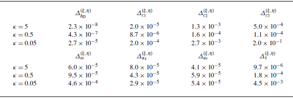


 Open access

