


1. Introduction
1.1. Objectives and background
Advances in transportation have increased mobility but also raised practical challenges such as elevated energy consumption and environmental impacts. Early work by von Kármán and Gabrielli highlighted a general trade-off between speed and propulsive efficiency (Gabrielli & von Kármán Reference Gabrielli and von Kármán1950); this trade-off motivates research into configurations that improve efficiency without large penalties in other domains. One such configuration is the wing-in-ground (WIG) effect: when a wing operates close to a solid or free surface, the lift-to-drag ratio can increase substantially (Fink Reference Fink1961; Ishizuka et al. Reference Ishizuka, Kohama, Kato and Yoshioka2006; Rozhdestvensky Reference Rozhdestvensky2006). Based on this effect, a WIG-based concept called the aero-train was proposed at Tohoku University and subsequently investigated by several authors (Kohama Reference Kohama2005; Yoon et al. Reference Yoon, Kohama, Kikuchi and Kato2006; Kikuchi et al. Reference Kikuchi, Ohta, Kato, Ishikawa and Kohama2007). The WIG configurations can thus offer improved aerodynamic performance at low clearances, but they also raise aeroacoustic concerns. Because operation is near the ground and often near populated areas, WIG systems may increase community noise exposure compared with conventional aircraft operating at cruise altitude (Moon et al. Reference Moon, Koh, Seo, Yoon and Cho2003; Ahmed, Takasaki & Kohama Reference Ahmed, Takasaki and Kohama2006).
More generally, aeroacoustic issues under WIG-like conditions are relevant beyond the aero-train concept: many wall-bounded lifting surfaces (e.g. high-lift devices, blade–tower interactions in wind farms) operate in regimes where near-wall flow features and ground proximity affect sound radiation. Understanding the mechanisms that couple the near-field flow to radiated noise in such configurations is therefore important for both fundamental aeroacoustics and practical noise mitigation.
In this study, we examine a NACA 4412 wing with imposed jet flow at several ground clearances to elucidate how WIG–jet interactions influence aeroacoustic generation. In particular, our objective is to identify the physical mechanisms by which vortex shedding and near-field hydrodynamic processes produce aeroacoustic noise, using a hydrodynamic (vortex–sound) perspective supported by high-fidelity simulation data.
(a) A von Kármán–Gabrielli diagram modified from the work of Gabrielli & von Kármán (Reference Gabrielli and von Kármán1950) and (b) Conceptual design of an aero-train based on the WIG effect.

1.2. Computational aeroacoustic method
It should be noted that the issue of aeroacoustic noise under the WIG effect has been previously studied by Lai et al. (Reference Lai, Tan, Zhu, Zhu and Obayashi2022, Reference Lai, Tan and Obayashi2023). However, these studies did not account for the influence of engine jet flows. Moreover, they employed a large-eddy simulations (LES) acoustic analogy hybrid method, which has limitations in accurately identifying noise sources. In hybrid methods, the sources are approximated using acoustic analogies, which separate the acoustic field into source and propagation components. This approach begins with far-field noise and traces it back to near-field origins, aiming to identify causative mechanisms. The development of acoustic analogy theory has progressively refined the localisation of noise sources – from far-field prediction to near-field identification, and ultimately to specific flow structures or behaviours responsible for sound generation.
Lighthill (Reference Lighthill1952, Reference Lighthill1954) introduced the first general formulation of acoustic analogy, known as Lighthill’s equation, which reformulates the Navier–Stokes equations into an inhomogeneous wave equation: $N ( q )=0\text{ }\Rightarrow \text{ }L ( q )=S ( q )$
, where
$N ( q )=0\text{ }\Rightarrow \text{ }L ( q )=S ( q )$
, where $N$
represents the Navier–Stokes operator,
$N$
represents the Navier–Stokes operator, $L$
is a linear wave operator, and
$L$
is a linear wave operator, and $S$
denotes the acoustic source term. This elegance comes at a cost: all propagation effects within the source region are lumped into the source term. Subsequent efforts have aimed to isolate genuine acoustic sources by separating propagating effects from non-radiating components (Phillips Reference Phillips1960; Colonius, Lele & Moin Reference Colonius, Lele and Moin1997). However, as noted by Wang, Freund & Lele (Reference Wang, Freund and Lele2006, pp. 486–487), this remains challenging: ‘The case of high-subsonic Mach number flow is particularly challenging due to the lack of clear scale separation. The flow and sound are difficult to separate in a meaningful way. In the application of acoustic analogies, this makes the designation of source terms versus propagation effects ambiguous at best.’
$S$
denotes the acoustic source term. This elegance comes at a cost: all propagation effects within the source region are lumped into the source term. Subsequent efforts have aimed to isolate genuine acoustic sources by separating propagating effects from non-radiating components (Phillips Reference Phillips1960; Colonius, Lele & Moin Reference Colonius, Lele and Moin1997). However, as noted by Wang, Freund & Lele (Reference Wang, Freund and Lele2006, pp. 486–487), this remains challenging: ‘The case of high-subsonic Mach number flow is particularly challenging due to the lack of clear scale separation. The flow and sound are difficult to separate in a meaningful way. In the application of acoustic analogies, this makes the designation of source terms versus propagation effects ambiguous at best.’
To some extent, the development of acoustic analogy theory has been about gradually narrowing the noise source region to smaller domains – from predicting far-field noise to identifying near-field noise and eventually pinpointing the specific flow structures or behaviours responsible for noise generation. Significant contributions to distinguishing radiating acoustic fields from non-radiating components were made by Goldstein and colleagues (Goldstein Reference Goldstein2005). In an unbounded quiescent fluid, a harmonic fluctuation with circular frequency $\omega$
takes the form
$\omega$
takes the form $f={{\rm e}^{{\rm i} ( \boldsymbol{k}\boldsymbol{\cdot }x+\omega t )}}$
, with wavenumber
$f={{\rm e}^{{\rm i} ( \boldsymbol{k}\boldsymbol{\cdot }x+\omega t )}}$
, with wavenumber $\text{ }k=\left | \boldsymbol{k} \right |$
. Only when
$\text{ }k=\left | \boldsymbol{k} \right |$
. Only when $k$
and
$k$
and $\omega$
satisfy the dispersion relation
$\omega$
satisfy the dispersion relation $k=\left | \omega /{{a}_{0}} \right |$
does the solution take the form of a radiating acoustic wave:
$k=\left | \omega /{{a}_{0}} \right |$
does the solution take the form of a radiating acoustic wave: $f={{\rm e}^{{\rm i}k ( \hat {\boldsymbol{k}}\boldsymbol{\cdot }x\pm {{a}_{0}}t )}},\ \hat {\boldsymbol{k}}=\boldsymbol{k}/k$
, which satisfies the homogeneous d’Alembert equation (Crighton Reference Crighton1981). By constructing a filter in
$f={{\rm e}^{{\rm i}k ( \hat {\boldsymbol{k}}\boldsymbol{\cdot }x\pm {{a}_{0}}t )}},\ \hat {\boldsymbol{k}}=\boldsymbol{k}/k$
, which satisfies the homogeneous d’Alembert equation (Crighton Reference Crighton1981). By constructing a filter in $(k,\omega)$
-space and transforming it to physical space, Goldstein derived equations that extract the radiating acoustic field, separating it from non-radiating components (Goldstein Reference Goldstein2009; Sinayoko, Agarwal & Hu Reference Sinayoko, Agarwal and Hu2011).
$(k,\omega)$
-space and transforming it to physical space, Goldstein derived equations that extract the radiating acoustic field, separating it from non-radiating components (Goldstein Reference Goldstein2009; Sinayoko, Agarwal & Hu Reference Sinayoko, Agarwal and Hu2011).
However, the filter based on the unbounded-fluid dispersion relation is not directly applicable to flows with solid boundaries. The development and validation of filters for transonic viscous flows remain ongoing challenges, and the finite window of the filtering operator introduces approximations. Even at best, where we can clearly isolate the radiating acoustic field, one fundamental question remains: what flow processes generate this acoustic source?
In light of these challenges, the present study adopts direct numerical simulations (DNS) to investigate the noise and flow behaviour of a wing under combined WIG and jet effects. The DNS solve the full compressible Navier–Stokes equations without approximation, directly capturing all physical quantities – including sound pressure – without relying on acoustic analogies or auxiliary equations. Leveraging the high-fidelity capability of DNS, we can accurately localise noise sources, and investigate the physical mechanisms that drive the generation of aeroacoustic noise.
1.3. Outline of the paper
This paper is organised as follows. In § 2, the boundary conditions and grid scheme are presented. In § 3, the results obtained for the wing under different clearances are presented. In § 4, the detailed mechanism of sound generation is discussed. We provide our conclusions in § 5.
2. Numerical procedure
2.1. Computational domain and boundary conditions
This study investigates the flow state and noise generation mechanism of an NACA 4412 wing under WIG–jet co-effect conditions at different ground clearances. The freestream Mach number is set to $M={{U}_{\alpha }}/{{a}_{\alpha }}=0.3$
, and the chord-based Reynolds number is defined as
$M={{U}_{\alpha }}/{{a}_{\alpha }}=0.3$
, and the chord-based Reynolds number is defined as $Re={{\rho }_{\alpha }}{{U}_{\alpha }}C/\mu =5\times {{10}^{4}}$
, where
$Re={{\rho }_{\alpha }}{{U}_{\alpha }}C/\mu =5\times {{10}^{4}}$
, where ${U}_{\alpha }$
is the uniform freestream velocity,
${U}_{\alpha }$
is the uniform freestream velocity, ${a}_{\alpha }$
,
${a}_{\alpha }$
, ${\rho }_{\alpha }$
and
${\rho }_{\alpha }$
and $C$
represent the speed of sound and density at infinity and chord length, respectively, and the viscosity
$C$
represent the speed of sound and density at infinity and chord length, respectively, and the viscosity $\mu$
is assumed to be constant. The variables are non-dimensionalised using
$\mu$
is assumed to be constant. The variables are non-dimensionalised using $C$
as the length scale,
$C$
as the length scale, ${a}_{\alpha }$
as the velocity scale, and
${a}_{\alpha }$
as the velocity scale, and ${\rho }_{\alpha }$
as the unit of density. Accordingly, the time scale is normalised as
${\rho }_{\alpha }$
as the unit of density. Accordingly, the time scale is normalised as $C/{{a}_{\alpha }}$
. The ground clearance is defined as the ratio of the height of the trailing edge from the ground to the chord length,
$C/{{a}_{\alpha }}$
. The ground clearance is defined as the ratio of the height of the trailing edge from the ground to the chord length, $H/C$
.
$H/C$
.
The jet flow is generated by applying a momentum source with a velocity profile, with the average jet velocity determined based on aero-train design parameters and set to $M=0.42$
. Considering the computational cost and the simplicity of the clean wing model, periodic boundary conditions are applied to the side walls, and the jet is treated as two-dimensional with a spanwise uniform velocity. A grid independence study was conducted to determine the spanwise domain size, which confirmed that a domain size
$M=0.42$
. Considering the computational cost and the simplicity of the clean wing model, periodic boundary conditions are applied to the side walls, and the jet is treated as two-dimensional with a spanwise uniform velocity. A grid independence study was conducted to determine the spanwise domain size, which confirmed that a domain size $0.2C$
in the spanwise direction is reasonable, which produces results for flow features and acoustic pressure indistinguishable from those obtained with larger spanwise sizes (details provided in Appendix B). The non-reflecting boundary conditions proposed by Poinsot & Lele (Reference Poinsot and Lele1992) are applied in this research at the outer boundary to prevent the waves reflecting from the boundary.
$0.2C$
in the spanwise direction is reasonable, which produces results for flow features and acoustic pressure indistinguishable from those obtained with larger spanwise sizes (details provided in Appendix B). The non-reflecting boundary conditions proposed by Poinsot & Lele (Reference Poinsot and Lele1992) are applied in this research at the outer boundary to prevent the waves reflecting from the boundary.
The present DNS were performed at $Re=5.0\times 10^{4}$
, which is appreciably below the full-scale Reynolds numbers typical of aero-train applications (order
$Re=5.0\times 10^{4}$
, which is appreciably below the full-scale Reynolds numbers typical of aero-train applications (order $10^{6}$
). This reduction is a deliberate compromise for three reasons.
$10^{6}$
). This reduction is a deliberate compromise for three reasons.
-
(i) Fully resolving all relevant flow and acoustic scales at $Re\sim 10^{6}$
with DNS is currently computationally infeasible for the domain sizes and the long time records required to obtain converged aeroacoustic spectra.
$Re\sim 10^{6}$
with DNS is currently computationally infeasible for the domain sizes and the long time records required to obtain converged aeroacoustic spectra. -
(ii) The present moderate-
$Re$
DNS reproduce the same qualitative flow features observed in our previous high-
$Re$
LES simulations (Lai et al. Reference Lai, Tan, Zhu, Zhu and Obayashi2022, Reference Lai, Tan and Obayashi2023) for the same configuration: periodic vortex formation on the suction surface, and vortex shedding at the trailing edge. -
(iii) The primary objective of the DNS is to clarify the qualitative physical mechanism of the vortex shedding
$\rightarrow$
oscillating force
$\rightarrow$
trailing-edge scattering pathway that generates narrowband tonal noise, not to provide quantitative engineering predictions at a specific Reynolds number. The DNS yield phase-accurate, high-fidelity flow and acoustic fields that are essential for explaining why periodic trailing-edge vortex shedding behaves as a strong dipole-type acoustic source – insight that is difficult to obtain with lower-resolution methods alone.


These consistent observations give us confidence that the mechanisms identified here are relevant to higher- $Re$
conditions for this configuration. Nevertheless, we explicitly acknowledge the limitation that while the mechanistic conclusions are expected to remain qualitatively valid, quantitative details (e.g. exact Strouhal numbers, sound pressure levels) may change at higher Reynolds numbers.
$Re$
conditions for this configuration. Nevertheless, we explicitly acknowledge the limitation that while the mechanistic conclusions are expected to remain qualitatively valid, quantitative details (e.g. exact Strouhal numbers, sound pressure levels) may change at higher Reynolds numbers.
2.2. Grid topology
We employ a non-uniform orthogonal grid in $X$
and
$X$
and $Y$
directions to meet the dual requirements of a sufficiently large computational domain to capture far-field acoustic waves and fine enough resolution to resolve boundary layer flows and detailed flow structures. In the
$Y$
directions to meet the dual requirements of a sufficiently large computational domain to capture far-field acoustic waves and fine enough resolution to resolve boundary layer flows and detailed flow structures. In the $Z$
direction, the grid is uniformly distributed with spacing
$Z$
direction, the grid is uniformly distributed with spacing $\Delta Z=0.0025C$
. The computational domain is divided into four regions, as shown in figure 2: (i) boundary layer region
$\Delta Z=0.0025C$
. The computational domain is divided into four regions, as shown in figure 2: (i) boundary layer region ${Z}_{bl}$
, (ii) vortex region
${Z}_{bl}$
, (ii) vortex region ${Z}_{v}$
, (iii) sound region
${Z}_{v}$
, (iii) sound region ${Z}_{s}$
, and (iv) buffer zone
${Z}_{s}$
, and (iv) buffer zone ${Z}_{bf}$
. The grid size in the boundary layer region is determined by (2.2) below (White & Xue Reference White and Xue2003), where
${Z}_{bf}$
. The grid size in the boundary layer region is determined by (2.2) below (White & Xue Reference White and Xue2003), where $\Delta S$
is the grid spacing,
$\Delta S$
is the grid spacing, ${U}_{\textit{fric}}$
is the friction velocity, and
${U}_{\textit{fric}}$
is the friction velocity, and ${\tau }_{wall}$
is the wall shear stress. In the vortex region, the grid size is set to match the Kolmogorov scale (
${\tau }_{wall}$
is the wall shear stress. In the vortex region, the grid size is set to match the Kolmogorov scale ( $\text{ }\!\eta \!\!\text{ }\propto R{{e}^{-( {3}/{4})}}$
) to resolve as much of the turbulent flow structure around the wing as possible. In the sound region, the grid spacing corresponds to the Taylor microscale (
$\text{ }\!\eta \!\!\text{ }\propto R{{e}^{-( {3}/{4})}}$
) to resolve as much of the turbulent flow structure around the wing as possible. In the sound region, the grid spacing corresponds to the Taylor microscale ( $\lambda\propto \textit{Re}^{- ({1}/{2})}$
) to ensure accurate sound wave propagation. In the buffer zone, despite the application of non-reflecting boundary conditions, weak reflection waves may still occur, leading to spurious sound waves that contaminate the data. Therefore, the grid size in this region is set to be relatively coarse to damp sound pressure, and the domain size is large enough to prevent wave reflections at the boundaries.
$\lambda\propto \textit{Re}^{- ({1}/{2})}$
) to ensure accurate sound wave propagation. In the buffer zone, despite the application of non-reflecting boundary conditions, weak reflection waves may still occur, leading to spurious sound waves that contaminate the data. Therefore, the grid size in this region is set to be relatively coarse to damp sound pressure, and the domain size is large enough to prevent wave reflections at the boundaries.
Set-up of the computational domain.

Grid spacing transitions smoothly between zones, and the difference between adjacent grid spacings is restricted to less than 5 % to ensure grid quality. The grid strategy has been validated with a mesh size independence study, showing that simulation with this grid strategy can accurately capture flow structures, peak frequency and acoustic wave propagation (see Appendix A). For $Re= 50\,000$
, the total grid number in this study is approximately 400 million. The sizes and grid resolutions of each part of the computational domain are summarised as follows:
$Re= 50\,000$
, the total grid number in this study is approximately 400 million. The sizes and grid resolutions of each part of the computational domain are summarised as follows:
 \begin{align} Z_{bl} & = \left \{ x\, \left |\, -1.1 \le x \le 0.1,\ \frac {H}{C} - 0.1 \le y \le 0.2 + \frac {H}{C} \right . \right \}\!,\quad \Delta x_{bl} \le 0.001C,\ \Delta y_{bl} \le 0.0005C; \nonumber \\ Z_{v} &= \left \{ x\, \left |\, 1.1 \le x \le 2.1,\ 0 \le y \le 0.45 + \frac {H}{C},\ x \notin Z_b \right . \right \}\!,\quad \Delta x_{v}, \Delta y_{v} \le 0.002C; \nonumber \\ Z_{s} &= \left \{ x\, \left |\, -12 \le x \le 12,\ 0 \le y \le 12,\ x \notin Z_b \cup Z_v \right . \right \}\!, \quad \Delta x_{s}, \Delta y_{s} \le 0.05C; \nonumber \\ Z_{bf} &= \left \{ x\, \left |\, -100 \le x \le 100,\ 0 \le y \le 100,\ x \notin Z_b \cup Z_v \cup Z_s \right . \right \}\!, \quad \Delta x_{bf}, \Delta y_{bf} \le 2C; \\[-28pt] \nonumber \end{align}
 \begin{align} \Delta S = \frac {y^+ \mu }{U_{\textit{fric}}\, \rho }, \quad U_{\textit{fric}} = \sqrt {\frac {\tau _{w\textit{all}}}{\rho }}, \quad \tau _{w\textit{all}} = \frac {C_f \rho U_\infty ^2}{2}, \quad C_f = \frac {0.026}{Re^{1/7}}. \\[-2pt] \nonumber \end{align}
2.3. Numerical method
The three-dimensional compressible Navier–Stokes equations with volume penalisation method are solved directly in this research:
 \begin{equation} \frac {\partial \rho }{\partial t}+\frac {\partial }{\partial {{x}_{j}}} ( \rho {{u}_{j}} )=-\left ( \frac {1}{\phi }-1 \right )\chi \frac {\partial }{\partial {{x}_{j}}} [ \rho ( {{u}_{j}}-{{U}_{0,j}} ) ], \end{equation}
 \begin{align} \frac {\partial \rho {{u}_{i}}}{\partial t}+\frac {\partial }{\partial {{x}_{j}}} ( \rho {{u}_{i}}{{u}_{j}} )=&-\frac {\partial p}{\partial {{x}_{i}}}+\frac {\partial {{\tau }_{\textit{ij}}}}{\partial {{x}_{j}}}-\frac {\chi }{\eta } ( {{u}_{i}}-{{U}_{0,i}} )\notag \\ &-{{u}_{i}}\left ( \frac {1}{\phi }-1 \right )\chi \frac {\partial }{\partial {{x}_{j}}} [ \rho ( {{u}_{j}}-{{U}_{0,j}} ) ], \end{align}
 \begin{align} \frac {\partial p}{\partial t}+ u_{j}\,\frac {\partial p}{\partial x_{j}}+ \gamma \,p\,\frac {\partial u_{j}}{\partial x_{j}}= (\gamma - 1)\!\left [\,\kappa \,\frac {\partial ^{2}T}{\partial x_{j}\,\partial x_{j}}+ \tau _{i j}\,\frac {\partial u_{i}}{\partial x_{j}}- \frac {\chi }{\eta _{T}}\,(T - T_{0}) \right ]\!, \\[10pt] \nonumber \end{align}
where $\rho$
is the density of the fluid,
$\rho$
is the density of the fluid, ${u}_{i}$
is the velocity,
${u}_{i}$
is the velocity, $p$
is the pressure, the viscous stress tensor is
$p$
is the pressure, the viscous stress tensor is ${{\tau }_{\textit{ij}}}=\mu (( {\partial {{u}_{i}}}/{\partial {{x}_{j}}})+( {\partial {{u}_{j}}}/{\partial {{x}_{i}}})-({2}/{3})( {\partial {{u}_{l}}}/{\partial {{x}_{l}}})\,{{\delta }_{\textit{ij}}} )$
,
${{\tau }_{\textit{ij}}}=\mu (( {\partial {{u}_{i}}}/{\partial {{x}_{j}}})+( {\partial {{u}_{j}}}/{\partial {{x}_{i}}})-({2}/{3})( {\partial {{u}_{l}}}/{\partial {{x}_{l}}})\,{{\delta }_{\textit{ij}}} )$
, $e$
is the total energy,
$e$
is the total energy, $T$
is the temperature,
$T$
is the temperature, ${U}_{0, i}$
and
${U}_{0, i}$
and ${T}_{0}$
are the velocity and the temperature of the rigid bodies, respectively,
${T}_{0}$
are the velocity and the temperature of the rigid bodies, respectively, $\phi$
is the porosity,
$\phi$
is the porosity, $\eta$
is the viscous permeability, and
$\eta$
is the viscous permeability, and ${\eta }_{T}$
is the thermal permeability. The thermal conductivity
${\eta }_{T}$
is the thermal permeability. The thermal conductivity $k$
is assumed to be constant. The Prandtl number
$k$
is assumed to be constant. The Prandtl number $\textit{Pr}=\gamma \mu /k$
is set to 0.72, where the ratio of the specific heats
$\textit{Pr}=\gamma \mu /k$
is set to 0.72, where the ratio of the specific heats $\gamma$
is set to 1.4. The fluid is assumed to be an ideal gas to close the equations; the equation of state reads
$\gamma$
is set to 1.4. The fluid is assumed to be an ideal gas to close the equations; the equation of state reads $p = \rho RT = ( \gamma -1 ) ( e - (1/2 ) \rho u_i u_i )$
, where
$p = \rho RT = ( \gamma -1 ) ( e - (1/2 ) \rho u_i u_i )$
, where $R$
is the gas constant. In the immersed boundary method with volume penalisation method, the boundaries between the fluid and the rigid bodies are identified by the mask function
$R$
is the gas constant. In the immersed boundary method with volume penalisation method, the boundaries between the fluid and the rigid bodies are identified by the mask function $\chi$
, defined by
$\chi$
, defined by
 \begin{equation} \chi (x, t) = \begin{cases} 1 & \text{if } x \in \text{rigid bodies}, \\ 0 & \text{otherwise}. \end{cases} \end{equation}
This equation indicates that the penalisation terms related to $\chi$
in (2.3)–(2.5) are only active within the solid region. In the fluid domain, the terms associated with
$\chi$
in (2.3)–(2.5) are only active within the solid region. In the fluid domain, the terms associated with $\chi$
vanish, reducing the system of equations to the standard compressible Navier–Stokes equations. The capability of this numerical method for simulating aeroacoustic problems has been validated by Komatsu, Iwakami & Hattori (Reference Komatsu, Iwakami and Hattori2016). The results showed that this method is suitable for various complex aeroacoustic simulations. Similar to the finite difference method used by Komatsu et al. (Reference Komatsu, Iwakami and Hattori2016), in this study, spatial derivatives are approximated by the sixth-order-accurate compact scheme except for the penalisation terms, which are approximated by the central finite difference of fourth-order accuracy. For time marching, the second-order implicit method is used for the penalisation terms, while the second-order explicit method is used for the other terms.
$\chi$
vanish, reducing the system of equations to the standard compressible Navier–Stokes equations. The capability of this numerical method for simulating aeroacoustic problems has been validated by Komatsu, Iwakami & Hattori (Reference Komatsu, Iwakami and Hattori2016). The results showed that this method is suitable for various complex aeroacoustic simulations. Similar to the finite difference method used by Komatsu et al. (Reference Komatsu, Iwakami and Hattori2016), in this study, spatial derivatives are approximated by the sixth-order-accurate compact scheme except for the penalisation terms, which are approximated by the central finite difference of fourth-order accuracy. For time marching, the second-order implicit method is used for the penalisation terms, while the second-order explicit method is used for the other terms.
3. Results and discussion
3.1. Flow states and aeroacoustic noise of the wing at different ground clearances and jet conditions
In this subsection, we analyse the flow states and aeroacoustic noise of an NACA 4412 wing at varying ground clearances and different jet conditions. Four simulation cases were conducted, as shown in table 1. These ground clearances fall within the typical range of the WIG effect, from $0.1C$
to
$0.1C$
to $1C$
. A no-jet case, C20_J0, was included to isolate the influence of jet flow on noise generation. To clarify the nomenclature: C10 denotes that clearance is 10 % of chord length
$1C$
. A no-jet case, C20_J0, was included to isolate the influence of jet flow on noise generation. To clarify the nomenclature: C10 denotes that clearance is 10 % of chord length $C$
, and J indicates jet status (1 active, 0 inactive). Since the jet influence was compared only for the C20 configuration (C20_J1 versus C20_J0), the J suffix is omitted for other clearance cases (C10, C40). This simplification preserves clarity while avoiding ambiguity in non-comparative scenarios. Given that lift and flow characteristics are more sensitive to clearance variations at lower ground clearances, we employed non-uniform increments in clearance to ensure a more detailed analysis in the most critical regions.
$C$
, and J indicates jet status (1 active, 0 inactive). Since the jet influence was compared only for the C20 configuration (C20_J1 versus C20_J0), the J suffix is omitted for other clearance cases (C10, C40). This simplification preserves clarity while avoiding ambiguity in non-comparative scenarios. Given that lift and flow characteristics are more sensitive to clearance variations at lower ground clearances, we employed non-uniform increments in clearance to ensure a more detailed analysis in the most critical regions.
Configuration of cases and corresponding aerodynamic performance. The time-averaged mean and standard deviation (STD) of $L/D$
are computed over the interval from 60 to 125 time units, corresponding to the period in which the flow is fully developed and exhibits an unsteady equilibrium state.
$L/D$
are computed over the interval from 60 to 125 time units, corresponding to the period in which the flow is fully developed and exhibits an unsteady equilibrium state.

As mentioned above, prior studies have not considered the effect of the jet. In this work, we incorporate the jet influence, bringing our conclusions one step closer to practical applications. We anticipate that the introduction of the jet-induced supercirculation effect will lead to a significant improvement in aerodynamic performance. Our results demonstrate that at angle of attack $5^\circ$
and ground clearance
$5^\circ$
and ground clearance $H/C=0.2$
, the inclusion of the jet increases
$H/C=0.2$
, the inclusion of the jet increases $L/D$
dramatically from 9.67 to 43.67; see table 1. More importantly, the introduction of the jet alters the trade-off between aerodynamic performance and aeroacoustic noise. As the ground clearance decreases, aerodynamic performance (
$L/D$
dramatically from 9.67 to 43.67; see table 1. More importantly, the introduction of the jet alters the trade-off between aerodynamic performance and aeroacoustic noise. As the ground clearance decreases, aerodynamic performance ( $L/D$
) improves, while the noise level decreases as well. At
$L/D$
) improves, while the noise level decreases as well. At $H/C=0.1$
, both the optimal aerodynamic and aeroacoustic performances are achieved under jet conditions.
$H/C=0.1$
, both the optimal aerodynamic and aeroacoustic performances are achieved under jet conditions.
Aeroacoustic noise, as a by-product of flow, inherently reflects the flow dynamics. Thus when discussing aeroacoustic noise, we are essentially examining the flow state. Before delving into the details of the acoustic field, we first present the flow state around the wing under different operating conditions. Figure 3 shows transient velocity contours at characteristic times for the NACA 4412 wing in different operating conditions.
Contours of the velocity field ( $U$
ranging from
$U$
ranging from $-0.05$
to 0.6) on the
$-0.05$
to 0.6) on the $Z=0$
plane under four operating conditions: (a) C40_J1, (b) C20_J1, (c) C10_J1, (d) C20_J0.
$Z=0$
plane under four operating conditions: (a) C40_J1, (b) C20_J1, (c) C10_J1, (d) C20_J0.

For all jet flow cases, vortex structures originate near the mid-chord and grow as they convect downstream. At relative high ground clearances (C20 and C40), stronger vortices develop, inducing secondary vortices that detach alternately at the trailing edge, forming a vortex street. However, at $H/C = 0.1$
, the vortices over the upper surface destabilise near the trailing edge, transitioning the wake into turbulence. For the case without a jet, the flow field would be quite different. The strong adverse pressure gradient near the trailing edge causes flow separation and recirculation (figure 3), consistent with the findings from Lai et al. (Reference Lai, Tan, Zhu, Zhu and Obayashi2022).
$H/C = 0.1$
, the vortices over the upper surface destabilise near the trailing edge, transitioning the wake into turbulence. For the case without a jet, the flow field would be quite different. The strong adverse pressure gradient near the trailing edge causes flow separation and recirculation (figure 3), consistent with the findings from Lai et al. (Reference Lai, Tan, Zhu, Zhu and Obayashi2022).
Overall, jet flow suppresses large-scale separation by promoting attached flow, shifting the dominant instability mechanism. It amplifies Tollmien–Schlichting (T–S) instability in the laminar boundary layer, generating boundary layer vortices. Without jet flow, however, shear between the recirculating and main flows develops to Kelvin–Helmholtz (K–H) instability in the separation region (see figure 4), generating large-scale but less coherent vortices. This shift in instability alters vortex evolution and significantly impacts aeroacoustic noise. The next subsection examines how these changes affect the acoustic field.
Figure 5 illustrates the vortex motion, development and noise radiation of the wing at $H/C=0.4$
at a characteristic time step. The grey background represents pressure fluctuations
$H/C=0.4$
at a characteristic time step. The grey background represents pressure fluctuations $P' = P - \bar {P}$
, where
$P' = P - \bar {P}$
, where $\bar {P}$
is the local time-averaged pressure obtained directly through DNS, while the coloured contours show vorticity. It is evident that trailing-edge noise is the dominant noise source in these cases. Movies in the (supplementary material is available at https://doi.org/10.1017/jfm.2025.11005) show that the generation of pressure waves is consistently accompanied by vortex shedding.
$\bar {P}$
is the local time-averaged pressure obtained directly through DNS, while the coloured contours show vorticity. It is evident that trailing-edge noise is the dominant noise source in these cases. Movies in the (supplementary material is available at https://doi.org/10.1017/jfm.2025.11005) show that the generation of pressure waves is consistently accompanied by vortex shedding.
To confirm that the observed pressure waves are indeed acoustic waves, we compared the pressure fluctuation ( $P'$
) data at two far-field observation points at
$P'$
) data at two far-field observation points at $(R_1, \theta ) = (8C, 90^\circ )$
and
$(R_1, \theta ) = (8C, 90^\circ )$
and $(R_2, \theta ) = (12C, 90^\circ )$
in the C40 case. The sound pressure amplitude at farther observation points was corrected using the sound pressure attenuation law
$(R_2, \theta ) = (12C, 90^\circ )$
in the C40 case. The sound pressure amplitude at farther observation points was corrected using the sound pressure attenuation law ${{P}_{1}}=\sqrt {{{{R}_{2}}}/{{{R}_{1}}}}\,{{P}_{2}}$
. Here, the pressure waves are treated as quasi-two-dimensional cylindrical waves. The time coordinates were corrected by the retarded time
${{P}_{1}}=\sqrt {{{{R}_{2}}}/{{{R}_{1}}}}\,{{P}_{2}}$
. Here, the pressure waves are treated as quasi-two-dimensional cylindrical waves. The time coordinates were corrected by the retarded time $({{R}_{2}}-{{R}_{1}})/{{a}_{\alpha }}$
. Figure 6 shows that the data from
$({{R}_{2}}-{{R}_{1}})/{{a}_{\alpha }}$
. Figure 6 shows that the data from ${R}_{1}$
and the corrected
${R}_{1}$
and the corrected ${R}_{2}$
match well, indicating that the pressure fluctuations follow the nature of sound wave propagation. These results provide evidence that the observed far-field pressure waves are indeed acoustic in nature, thereby enabling the extraction of acoustic field characteristics with little contamination from hydrodynamic disturbances.
${R}_{2}$
match well, indicating that the pressure fluctuations follow the nature of sound wave propagation. These results provide evidence that the observed far-field pressure waves are indeed acoustic in nature, thereby enabling the extraction of acoustic field characteristics with little contamination from hydrodynamic disturbances.
Dominant flow instability governing the flow state with and without the jet at C20 (showing the $U$
component): (a) K–H instability in the free shear layer in separation region (no jet); (b) T–S instability in the boundary layer (with jet).
$U$
component): (a) K–H instability in the free shear layer in separation region (no jet); (b) T–S instability in the boundary layer (with jet).

Vortex structure coloured by vorticity magnitude (upper image), with the dilation field in greyscale background (lower image) at a characteristic time step on the Z = 0 plane in case C40. The vortex and sound curve indicate the positions used for data extraction in the following analysis.

Comparison of time history of pressure at $(R, \theta ) = (8C, 90^\circ )$
(solid line) and corrected time history of pressure at
$(R, \theta ) = (8C, 90^\circ )$
(solid line) and corrected time history of pressure at $(R, \theta ) = (12C, 90^\circ )$
(dashed line) of C10.
$(R, \theta ) = (12C, 90^\circ )$
(dashed line) of C10.

Figure 7 shows the pressure amplitude spectra at the far-field observation point $(R, \theta ) = (12C, 90^\circ )$
under different ground clearances and jet conditions. The time series used for spectral analysis covered the interval
$(R, \theta ) = (12C, 90^\circ )$
under different ground clearances and jet conditions. The time series used for spectral analysis covered the interval $T \in [40,125]$
with time step
$T \in [40,125]$
with time step $\Delta t=5\times 10^{-4}$
. Employing a long time history improved the signal-to-noise ratio, allowing for clear isolation of the tone. Vortex sound theory underscores the critical role of vortex strength in generating aeroacoustic noise; as expected, stronger trailing vortices at higher ground clearances correspond to noticeably increased sound pressure amplitudes, whereas both the C10 and C20_J0 cases exhibit lower noise levels due to their relatively weak vortex strength at the trailing edge. The noise level – or equivalently, the vortex strength – is influenced by both the ground clearance and the jet condition.
$\Delta t=5\times 10^{-4}$
. Employing a long time history improved the signal-to-noise ratio, allowing for clear isolation of the tone. Vortex sound theory underscores the critical role of vortex strength in generating aeroacoustic noise; as expected, stronger trailing vortices at higher ground clearances correspond to noticeably increased sound pressure amplitudes, whereas both the C10 and C20_J0 cases exhibit lower noise levels due to their relatively weak vortex strength at the trailing edge. The noise level – or equivalently, the vortex strength – is influenced by both the ground clearance and the jet condition.
Changes in ground clearance not only affect noise intensity but also shift the peak frequency. For higher ground clearances with jet ( $H/C \geq 0.2$
), the dominant non-dimensional noise frequency is close to 1; however, when the ground clearance is reduced to
$H/C \geq 0.2$
), the dominant non-dimensional noise frequency is close to 1; however, when the ground clearance is reduced to $H/C = 0.1$
, the peak frequency abruptly drops to approximately 0.4. This sudden shift is closely related to the early breakdown of vortex structures. We will elaborate on this later in this section.
$H/C = 0.1$
, the peak frequency abruptly drops to approximately 0.4. This sudden shift is closely related to the early breakdown of vortex structures. We will elaborate on this later in this section.
The impact of the jet on aeroacoustic noise is particularly pronounced. While separation–stall noise is generally much stronger than noise associated with laminar flow (Brooks, Pope & Marcolini Reference Brooks, Pope and Marcolini1989), our findings reveal a contrasting scenario: the introduction of a jet transforms a flow that would otherwise exhibit massive separation into an attached flow, yet paradoxically results in a substantial increase in aerodynamic noise. By modulating the flow behaviour, the jet effectively converts the separation–stall noise observed in the no-jet case into laminar boundary layer vortex shedding (LBL-VS) noise. Given that separation–stall noise has been extensively investigated in previous studies (Lacagnina et al. Reference Lacagnina2019; Amirsalari & Rocha Reference Amirsalari and Rocha2023), including in the context of the ground effect (Lai et al. Reference Lai, Tan, Zhu, Zhu and Obayashi2022), the present work focuses primarily on the mechanisms and characteristics of LBL-VS noise induced by the jet.
Spectrum of sound pressure at $(R, \theta ) = (12C, 90^\circ )$
with four different operating conditions: (a,b,c,d) are C10_J1, C20_J1, C40_J1 and C20_J0, respectively. Spectra were estimated using Welch’s method: the time series was split into eight segments of length
$(R, \theta ) = (12C, 90^\circ )$
with four different operating conditions: (a,b,c,d) are C10_J1, C20_J1, C40_J1 and C20_J0, respectively. Spectra were estimated using Welch’s method: the time series was split into eight segments of length $T_{\textit{seg}}\approx 37\,778$
, with 50 % overlap, windowed by a Hanning window, and averaged to obtain the power spectral density (PSD, in dB). The frequency resolution is
$T_{\textit{seg}}\approx 37\,778$
, with 50 % overlap, windowed by a Hanning window, and averaged to obtain the power spectral density (PSD, in dB). The frequency resolution is $\Delta f = 1 / T_{{seg}}$
, and the Nyquist frequency is
$\Delta f = 1 / T_{{seg}}$
, and the Nyquist frequency is $f_{\textit{Nyquist}} = 1 / (2\, \Delta t)$
. The 95 % confidence interval is shown in the grey band.
$f_{\textit{Nyquist}} = 1 / (2\, \Delta t)$
. The 95 % confidence interval is shown in the grey band.

3.2. Intermittent phenomenon
Figure 8 shows the pressure footprint of vortices and sound waves on the upper surface of the wing. The horizontal axis represents the simulation time $T$
, while the vertical axis corresponds to chordwise stations along the vortex curve as shown in figure 5. Here, pressure rather than vorticity is used to represent vortex structures. This is because small variations in measurement locations can result in significant changes in vorticity, which may also be influenced by shear flow in the boundary layer where vorticity is high but no vortices are present. On the other hand, pressure can contain information simultaneously about both vortices and sound. In figure 8, the dark blue streaks represent the negative pressure footprints of vortices. The positive slope
$T$
, while the vertical axis corresponds to chordwise stations along the vortex curve as shown in figure 5. Here, pressure rather than vorticity is used to represent vortex structures. This is because small variations in measurement locations can result in significant changes in vorticity, which may also be influenced by shear flow in the boundary layer where vorticity is high but no vortices are present. On the other hand, pressure can contain information simultaneously about both vortices and sound. In figure 8, the dark blue streaks represent the negative pressure footprints of vortices. The positive slope $k^+$
indicates the downstream convection speed of these vortices, which is approximately 0.25. This velocity is slightly lower than that of the mainstream flow due to the blocking effect of the boundary layer. Similarly, the light yellow streaks correspond to the positive pressure footprints of sound waves, with their negative slope
$k^+$
indicates the downstream convection speed of these vortices, which is approximately 0.25. This velocity is slightly lower than that of the mainstream flow due to the blocking effect of the boundary layer. Similarly, the light yellow streaks correspond to the positive pressure footprints of sound waves, with their negative slope $k^-$
signifying the upstream propagation of sound waves originating from the trailing edge (TE). The speed of sound
$k^-$
signifying the upstream propagation of sound waves originating from the trailing edge (TE). The speed of sound ${{u}_{s}}\approx 0.55$
, as shown in figure 8(b), over the wing is significantly lower than unity due to the combined influence of reduced density, the high-speed background flow near the leading edge (LE), and curvature effects.
${{u}_{s}}\approx 0.55$
, as shown in figure 8(b), over the wing is significantly lower than unity due to the combined influence of reduced density, the high-speed background flow near the leading edge (LE), and curvature effects.
Figure 8 confirms our earlier observation: each time a vortex sheds from the trailing edge (as indicated by dark blue streaks with positive slope reaching the trailing edge at $C=1$
), a pressure fluctuation (light yellow streaks with negative slope originating at
$C=1$
), a pressure fluctuation (light yellow streaks with negative slope originating at $C=1$
) is generated and propagates upstream. However, upon closer inspection, an intermittent phenomenon can be observed in the C10 case. Namely, the corresponding acoustic field exhibits a periodic alternation between short, intense ‘noisy’ bursts and prolonged ‘silent’ intervals, occurring at a frequency significantly lower than the natural vortex shedding frequency. This is because in C10, vortices – except those amplified by the acoustic waves – are relatively weak and fail to convect downstream and shed at the trailing edge. As a result, their pressure footprints seem to ‘disappear’ near the trailing edge.
$C=1$
) is generated and propagates upstream. However, upon closer inspection, an intermittent phenomenon can be observed in the C10 case. Namely, the corresponding acoustic field exhibits a periodic alternation between short, intense ‘noisy’ bursts and prolonged ‘silent’ intervals, occurring at a frequency significantly lower than the natural vortex shedding frequency. This is because in C10, vortices – except those amplified by the acoustic waves – are relatively weak and fail to convect downstream and shed at the trailing edge. As a result, their pressure footprints seem to ‘disappear’ near the trailing edge.
Spatial–temporal pressure footprint of vortex and sound wave (a) with intermittent phenomenon in C10, and (b) without intermittent phenomenon in C40. The red dashed arrows represent the trace of the upstream-propagating sound wave, and the blue solid arrows represent the trace of the downstream-convecting vortex. The horizontal dashed line indicates the station of unstable region, relative to the chord length, where the instability induced by sound wave grows to the same order of hydrodynamic pressure. Vortex and sound signals are recorded along the vortex and sound curves, respectively (see figure 5). Here S and E are stand for the Start and End of the sound-vortex feedback, respectively.

The intermittent phenomenon occurs because at lower ground clearances, the flow state around the wing undergoes significant changes. A strong pressure near the trailing edge builds up a formidable adverse pressure gradient, significantly impacting the upstream flow in the vicinity of the trailing edge. Compared to C40, the vortex evolution pattern over the aerofoil in C10 exhibits a completely different mode, as shown in figure 9, which can be divided into two distinct stages: the growth stage and the dissipation stage. During the growth stage, the shear layer in the boundary layer rolls up under the influence of disturbances, leading to the diffusion of vorticity originally concentrated within the highly sheared boundary layer. This diffusion, combined with the shear effects of the main flow, results in the formation of well-organised, large-scale vortices. While the growth stage is essentially similar between C10 and C40, their dissipation stages exhibit significant differences. In C40, the relatively low pressure, yet still high, near the trailing edge allows a balance between diffusion and pressure effects, preventing severe vortex compression. As a result, the energy dissipation rate remains low, and nearly all vortex structures can pass through the high-pressure region intact before shedding at the trailing edge. In contrast, the scenario in C10 is markedly different. At such a low ground clearance, a stronger high-pressure region forms near the trailing edge. When vortices approach this high-pressure zone, they enter the dissipation stage, during which the vortices contract due to the high pressure, causing vorticity to concentrate towards the vortex core. The conservation of angular momentum further amplifies the vorticity. As the vorticity becomes highly concentrated, viscous effects become significant, leading to the rapid dissipation and breakdown of vortex energy; see figures 9 and 10.
The vortices evolution pattern over the aerofoil on the $Z=0$
plane in C40 (left) and C10 (right) is shown by colour. The solid line shows the trajectory of the vortex that can be shed from the trailing edge; the long-dashed line in C40 indicates the development of a vortex, while in C10 it shows the shrinkage and breakdown of the vortex. The dotted line separates the growth stage from the dissipation stage of vortex evolution.
$Z=0$
plane in C40 (left) and C10 (right) is shown by colour. The solid line shows the trajectory of the vortex that can be shed from the trailing edge; the long-dashed line in C40 indicates the development of a vortex, while in C10 it shows the shrinkage and breakdown of the vortex. The dotted line separates the growth stage from the dissipation stage of vortex evolution.

The energy dissipation mode of the C10 (dashed line, triangles) and C40 (solid line, squares) cases is shown. The time-averaged magnitude of $\varepsilon ^*$
is calculated on the vortex curve and normalised by each maximum. Here,
$\varepsilon ^*$
is calculated on the vortex curve and normalised by each maximum. Here, $C = 0$
represents the leading edge, and
$C = 0$
represents the leading edge, and $C = 1$
the trailing edge.
$C = 1$
the trailing edge.

As shown in figure 10, the comparison between the energy dissipation modes of flows with vortex breakdown (C10) and without breakdown (C40) reveals distinct trends; the normalised time-averaged magnitude of the dissipation rate is given by
 \begin{equation} {{\varepsilon }^{*}}={\varepsilon }/{{{\varepsilon }_{\textit{max}}}}, \end{equation}
where $\varepsilon =2\nu\, \overline {{{S}_{\textit{ij}}}{{S}_{\textit{ij}}}}$
, and
$\varepsilon =2\nu\, \overline {{{S}_{\textit{ij}}}{{S}_{\textit{ij}}}}$
, and ${S}_{\textit{ij}}$
is the strain rate tensor, calculated on the vortex curve in figure 5. In both cases, a peak occurs near the mid-chord due to the generation of a positive vortex sheet. However, a notable discrepancy in energy dissipation rates emerges further downstream. In the C40 case, the dissipation rate decreases after the peak and remains relatively low, whereas in the C10 case, the dissipation rate keeps a relatively high level and exhibits a sharp increase near the trailing edge. The increased dissipation rate corresponds to the regions where most of the vortices undergo breakdown. As a result, in the C10 case, most of the spanwise vortices destabilise and break down into smaller vortex structures, exhibiting turbulent characteristics.
${S}_{\textit{ij}}$
is the strain rate tensor, calculated on the vortex curve in figure 5. In both cases, a peak occurs near the mid-chord due to the generation of a positive vortex sheet. However, a notable discrepancy in energy dissipation rates emerges further downstream. In the C40 case, the dissipation rate decreases after the peak and remains relatively low, whereas in the C10 case, the dissipation rate keeps a relatively high level and exhibits a sharp increase near the trailing edge. The increased dissipation rate corresponds to the regions where most of the vortices undergo breakdown. As a result, in the C10 case, most of the spanwise vortices destabilise and break down into smaller vortex structures, exhibiting turbulent characteristics.
Interestingly, the intermittent phenomenon suggests that although most vortices break down in C10, a minority still periodically shed, indicating that vortex strength is periodically enhanced. This is because only when the vortex is sufficiently robust to survive the dissipation process in the high-pressure region can it shed and generate a burst of sound waves. In the next subsection, we elucidate the mechanism behind these vortex strength fluctuations, with particular emphasis on the feedback effects of sound waves.
3.3. Feedback phenomenon
The introduction of the jet causes the noise generation mechanism of the wing under the WIG effect to shift from separation noise to LBL-VS noise. A key feature of LBL-VS noise is that its intensity and frequency are influenced by the feedback of sound waves (Brooks et al. Reference Brooks, Pope and Marcolini1989; Thurman, Zawodny & Pettingill Reference Thurman, Zawodny and Pettingill2022). Thanks to high-fidelity DNS, we have observed a remarkably clear sound wave feedback loop in this study. Specifically, we can directly see how sound waves influence vortex formation. Sound waves feed back onto unstable regions, amplifying the strength of vortex ‘seeds’. As stronger vortices shed, they generate more intense sound waves, reinforcing a positive feedback loop. To show the effect of sound waves on vortex intensity, figure 11 presents the correlation coefficient maps between the sound and vortex intensities at different chordwise stations. The cross-correlation is calculated by
 \begin{equation} {{R}_{\textit{s}v}}(T)=\underset {n}{\overset {{}}{\mathop \sum }}\,{{f}_{s}}\left ( n \right )\,{{f}_{v}}\left ( T+n \right )\!, \\[-10pt] \nonumber \end{equation}
 \begin{equation} {{r}_{\textit{s}v}}=\frac {{{R}_{\textit{s}v}}(0)}{\sqrt {{{R}_{ss}}(0)\,{{R}_{vv}}(0)}}, \\[12pt] \nonumber \end{equation}
where ${{R}_{\textit{s}v}}(T)$
and
${{R}_{\textit{s}v}}(T)$
and ${r}_{\textit{s}v}$
are cross-correlation function and correlation coefficient, respectively. The time histories of pressures
${r}_{\textit{s}v}$
are cross-correlation function and correlation coefficient, respectively. The time histories of pressures ${{f}_{s}} ( T )$
and
${{f}_{s}} ( T )$
and ${{f}_{v}} ( T )$
, caused by sound and vortex, respectively, were extracted from the corresponding sound and vortex curves, as shown in figure 5. In the region unaffected by vortex-induced hydrodynamic pressure – specifically region A where the station on the vortex curve is
${{f}_{v}} ( T )$
, caused by sound and vortex, respectively, were extracted from the corresponding sound and vortex curves, as shown in figure 5. In the region unaffected by vortex-induced hydrodynamic pressure – specifically region A where the station on the vortex curve is $Cv\lt 0.3$
– there is a significant correlation between the pressures on the vortex curve and on the entire sound curve. Additionally, the correlation coefficient map in this region exhibits a pattern with positive slope
$Cv\lt 0.3$
– there is a significant correlation between the pressures on the vortex curve and on the entire sound curve. Additionally, the correlation coefficient map in this region exhibits a pattern with positive slope ${{k}_{\textit{same}}}={{u}_{s,Cs}}/{{u}_{s,Cv}}\approx 1$
, indicating that pressures on the sound and vortex curves maintain the same phase and propagate in the same direction. This observation is intuitive, as the pressure fluctuations measured along the sound and vortex curves in this region are both primarily caused by in-phase sound waves.
${{k}_{\textit{same}}}={{u}_{s,Cs}}/{{u}_{s,Cv}}\approx 1$
, indicating that pressures on the sound and vortex curves maintain the same phase and propagate in the same direction. This observation is intuitive, as the pressure fluctuations measured along the sound and vortex curves in this region are both primarily caused by in-phase sound waves.
Cross-correlation coefficients map between points on the vortex curve ( $Cv$
) and the sound curve (
$Cv$
) and the sound curve ( $Cs$
) at C10. The leading edge is defined as the station where
$Cs$
) at C10. The leading edge is defined as the station where $Cv$
or
$Cv$
or $Cs$
equals 0, while the trailing edge is characterised by value 1. Here,
$Cs$
equals 0, while the trailing edge is characterised by value 1. Here, ${{k}_{\textit{same}}}={{u}_{s,Cs}}/{{u}_{s,Cv}}\approx 1$
is the slope of the pattern in region A, indicating the in-phase pressure on
${{k}_{\textit{same}}}={{u}_{s,Cs}}/{{u}_{s,Cv}}\approx 1$
is the slope of the pattern in region A, indicating the in-phase pressure on $Cv$
and
$Cv$
and $Cs$
;
$Cs$
; ${{k}_{\textit{re}v\textit{erse}}}={{u}_{s,Cs}}/{{u}_{v,Cv}}\approx 2.2$
is the negative slope of the pattern in region B, indicating the speed ratio of upgoing sound wave and downgoing vortex.
${{k}_{\textit{re}v\textit{erse}}}={{u}_{s,Cs}}/{{u}_{v,Cv}}\approx 2.2$
is the negative slope of the pattern in region B, indicating the speed ratio of upgoing sound wave and downgoing vortex.

However, when moving downstream (i.e. for $Cv\gt 0.3$
), disturbances from the vortices cause significant changes. The correlation between the sound curve data and the vortex curve data drops sharply, becoming quite weak in vicinity of the trailing edge. Nevertheless, a clear striped pattern with a regular negative slope is still observable in the region B defined by
$Cv\gt 0.3$
), disturbances from the vortices cause significant changes. The correlation between the sound curve data and the vortex curve data drops sharply, becoming quite weak in vicinity of the trailing edge. Nevertheless, a clear striped pattern with a regular negative slope is still observable in the region B defined by $Cs\lt 0.5$
and
$Cs\lt 0.5$
and $0.3\lt Cv\lt 0.6$
, as shown in figure 11. The negative slope in this region indicates that as an observation point along the vortex curve moves downstream to trace a vortex, the corresponding correlated signal on the sound curve is detected at an upstream location. This occurs because the two ‘signal carriers’, vortex and sound wave, propagate in opposite directions: the vortex structures, which are enhanced by the sound wave, convect downstream, while the sound wave continues to travel upstream. If we examine the sound wave propagation speed and the vortex convection speed (by the slope of the pressure footprint in figure 8), then we find that their respective speeds are
$0.3\lt Cv\lt 0.6$
, as shown in figure 11. The negative slope in this region indicates that as an observation point along the vortex curve moves downstream to trace a vortex, the corresponding correlated signal on the sound curve is detected at an upstream location. This occurs because the two ‘signal carriers’, vortex and sound wave, propagate in opposite directions: the vortex structures, which are enhanced by the sound wave, convect downstream, while the sound wave continues to travel upstream. If we examine the sound wave propagation speed and the vortex convection speed (by the slope of the pressure footprint in figure 8), then we find that their respective speeds are ${u}_{s} = 0.55$
and
${u}_{s} = 0.55$
and ${u}_{v} = 0.25$
, with speed ratio approximately 2.2, which matches well with the negative slope
${u}_{v} = 0.25$
, with speed ratio approximately 2.2, which matches well with the negative slope ${{k}_{\textit{re}v\textit{erse}}}={{u}_{s, Cs}}/{{u}_{v, Cv}}$
in region B.
${{k}_{\textit{re}v\textit{erse}}}={{u}_{s, Cs}}/{{u}_{v, Cv}}$
in region B.
These findings demonstrate the mechanism of sound wave feedback acting on the flow instability or vortex formation in correlation aspect. Specifically, when these waves, generated at the trailing edge, pass through the unstable region (around $Cv=0.3$
), they amplify the instability in that region and imprint a sound wave footprint on the subsequent vortex formation. This explains why the pattern near
$Cv=0.3$
), they amplify the instability in that region and imprint a sound wave footprint on the subsequent vortex formation. This explains why the pattern near $Cv=0.3$
exhibits both positive and negative slopes on the left- and right-hand sides, respectively. It also indicates that at
$Cv=0.3$
exhibits both positive and negative slopes on the left- and right-hand sides, respectively. It also indicates that at $X/C=0.3$
, the instability induced by acoustic perturbations grows to the same order as the hydrodynamic pressure and thus becomes observable. We emphasise, however, that this does not imply that the instability originates at
$X/C=0.3$
, the instability induced by acoustic perturbations grows to the same order as the hydrodynamic pressure and thus becomes observable. We emphasise, however, that this does not imply that the instability originates at $X/C=0.3$
; rather, it is simply the location where it can be detected. To further illustrate the effect of sound–vortex interactions, it is natural to check if the dominant noise frequency corresponds to the frequency of sound feedback. Hence we calculate the sound feedback period as
$X/C=0.3$
; rather, it is simply the location where it can be detected. To further illustrate the effect of sound–vortex interactions, it is natural to check if the dominant noise frequency corresponds to the frequency of sound feedback. Hence we calculate the sound feedback period as
 \begin{equation} {{T}_{F}}={{t}_{s}}+{{t}_{v}}+{{t}_{sr}}+{{t}_{vr}}, \end{equation}
where ${T}_{F}$
represents the feedback cycle,
${T}_{F}$
represents the feedback cycle, ${t}_{s}$
is the sound propagation time,
${t}_{s}$
is the sound propagation time, ${t}_{v}$
is the vortex convection time, and
${t}_{v}$
is the vortex convection time, and ${t}_{sr}$
is the time delay due to the receptivity of sound wave to vortex formation (Gojon et al. Reference Gojon, Bauerheim, Fiore and Moreau2024). The latter simply corresponds to the time difference between the vortex reaching the trailing edge and the sound wave starting to propagate from the trailing edge, as shown in figure 8. Similarly,
${t}_{sr}$
is the time delay due to the receptivity of sound wave to vortex formation (Gojon et al. Reference Gojon, Bauerheim, Fiore and Moreau2024). The latter simply corresponds to the time difference between the vortex reaching the trailing edge and the sound wave starting to propagate from the trailing edge, as shown in figure 8. Similarly, ${t}_{vr}$
is the time delay due to the receptivity of vortex in generating sound, which is the time difference between the sound wave reaching the unstable region and the vortex starting to form from that region. Both
${t}_{vr}$
is the time delay due to the receptivity of vortex in generating sound, which is the time difference between the sound wave reaching the unstable region and the vortex starting to form from that region. Both ${t}_{sr}$
and
${t}_{sr}$
and ${t}_{vr}$
are values averaged over multiple periods. The schematic of sound–vortex feedback interaction is shown in figure 12. For the C10 case, the feedback cycle is approximately 4.8 time units, shown as follows:
${t}_{vr}$
are values averaged over multiple periods. The schematic of sound–vortex feedback interaction is shown in figure 12. For the C10 case, the feedback cycle is approximately 4.8 time units, shown as follows:
 \begin{align} {{T}_{F}}&=\frac {\Delta C}{{{u}_{s}}}+\frac {\Delta C}{{{u}_{v}}}+{{t}_{sr}}+{{t}_{vr}} \nonumber \\[2pt] &\approx \frac {1-0.3}{0.55}+\frac {1-0.3}{0.25}+0.7+0.1\approx 4.8. \end{align}
Sketch of sound–vortex feedback loop, where ${P}_{v}$
represents the hydrodynamic pressure induced by vortices convected downstream at velocity
${P}_{v}$
represents the hydrodynamic pressure induced by vortices convected downstream at velocity ${u}_{v}$
, while
${u}_{v}$
, while ${P}_{s}$
denotes the sound pressure propagating at the local sound speed
${P}_{s}$
denotes the sound pressure propagating at the local sound speed ${u}_{s}$
, generated during vortex shedding. The reception behaviour
${u}_{s}$
, generated during vortex shedding. The reception behaviour ${\delta }_{vr}$
describes the conversion of vortices into sound, whereas
${\delta }_{vr}$
describes the conversion of vortices into sound, whereas ${\delta }_{sr}$
represents the reverse process of sound influencing vortex generation.
${\delta }_{sr}$
represents the reverse process of sound influencing vortex generation.

Time history of pressure fluctuations near trailing edge $(X,Y) = (0.05,0.1)$
of C10, where RMS indicates the root mean square value, A1 is the RMS value calculated from all absolute pressure values below the RMS threshold, and A2 is the RMS value of all peaks above this threshold. All of RMS, A1 and A2 are multiplied by a negative sign to facilitate comparison.
$(X,Y) = (0.05,0.1)$
of C10, where RMS indicates the root mean square value, A1 is the RMS value calculated from all absolute pressure values below the RMS threshold, and A2 is the RMS value of all peaks above this threshold. All of RMS, A1 and A2 are multiplied by a negative sign to facilitate comparison.

Frequency spectra reveal that the peak frequency 0.42 of case C10 is exactly twice the expected value. This is because overlapping alternating feedback loops are generated (see figure 8 a), resulting in the observed fluctuation period at the measuring point being approximately half of the actual feedback loop period. Clearly, the intermittent phenomenon occurs because some vortices, periodically amplified by sound waves, are able to shed from the trailing edge without breakdown, even after passing through the high-pressure region.
Figure 13 shows the pressure time history at the trailing edge of the wing in the C10 case. The root mean square (RMS) value A2 of pressure amplitude represents the effective pressure fluctuations from vortices that are amplified by the sound wave, while A1 represents the pressure fluctuations without sound amplification. The value of A2 is more than twice that of A1. The high amplitude peaks correspond to stronger vortices enhanced by sound waves, which correspond to the dark blue streak in figure 8. As demonstrated in the preceding discussion, there is indeed a feedback effect of sound waves that enhances flow instability. This leading-edge instability, triggered by the acoustic wave within the feedback loop, was also investigated by Ricciardi, Wolf & Taira (Reference Ricciardi, Wolf and Taira2022) using the resolvent method, which provides a clear input–output characterisation of the loop. The present results reveal a feedback process that is closely consistent with their findings.
4. Noise generation mechanism
4.1. Noise generation in the process of vorticity transfer around the trailing edge
In this subsection, we detail the noise generation mechanism of a wing under the WIG–jet co-effect. From the preceding analysis, we observed that sound waves are consistently generated when strong spanwise vortex structures shed from the trailing edge. Although trailing-edge noise has been studied extensively (Lee et al. Reference Lee, Ayton, Bertagnolio, Moreau, Chong and Joseph2021), including theoretical analyses (Crighton Reference Crighton1972; Möhring Reference Möhring1978; Goldstein Reference Goldstein2005) and quantitative predictions (Sandberg, Sandham & Joseph Reference Sandberg, Sandham and Joseph2007; Kojima et al. Reference Kojima, Skene, Yeh, Taira and Kameda2023), there is still no clear consensus on the physical mechanisms by which vortices interact with the edge to produce intense noise, particularly from a hydrodynamic perspective – i.e. how the shedding vortices locally accelerate the flow, induce strong vorticity variations, and thereby act as effective noise sources. As noted earlier, even under favourable conditions where hydrodynamic and acoustic pressures can be cleanly separated (Goldstein Reference Goldstein2009; Sinayoko et al. Reference Sinayoko, Agarwal and Hu2011), fully elucidating the processes underlying aeroacoustic noise generation remains a significant challenge.
Time history of sound source magnitude $\boldsymbol{\nabla }\boldsymbol{\cdot }( \rho \boldsymbol{\omega } \times \boldsymbol{u} )$
(red line) and pressure fluctuation
$\boldsymbol{\nabla }\boldsymbol{\cdot }( \rho \boldsymbol{\omega } \times \boldsymbol{u} )$
(red line) and pressure fluctuation ${P}'$
(blue line) at the centre of the vorticity transfer region (sound source region) of C40.
${P}'$
(blue line) at the centre of the vorticity transfer region (sound source region) of C40.

Therefore, we employ high-fidelity DNS data to directly extract the acoustic field ( ${P}' = P - \bar {P}$
) and apply vortex sound theory to evaluate the noise sources within the flow, with the aim of uncovering the physical processes underlying noise generation. Powell et al. (Reference Powell1964) introduced the concept of vortex sound theory, asserting that unsteady vortex motion is the primary source of aeroacoustic noise in vortex flow. Within the framework of Lighthill’s theory, they derived the vortex sound equation
${P}' = P - \bar {P}$
) and apply vortex sound theory to evaluate the noise sources within the flow, with the aim of uncovering the physical processes underlying noise generation. Powell et al. (Reference Powell1964) introduced the concept of vortex sound theory, asserting that unsteady vortex motion is the primary source of aeroacoustic noise in vortex flow. Within the framework of Lighthill’s theory, they derived the vortex sound equation
 \begin{equation} \left ( \frac {1}{{{c}^{2}}}\partial _{t}^{2}-{{{\nabla} }^{2}} \right ){P}'=\boldsymbol{\nabla }\boldsymbol{\cdot }\left ( \rho \boldsymbol{\omega } \times \boldsymbol{u} \right )\!, \end{equation}
in which Lighthill’s stress tensor is simplified into the nonlinear Lamb vector, which represents a dipole source. This dipole source generates sound waves only when $\partial_t (\rho \boldsymbol{\omega } \times \boldsymbol{u} )\ne 0$
. It should be noted that (4.1) is derived from Lighthill’s equation and is therefore, strictly speaking, a free-space approximation. Nevertheless, it is a reasonable approximation in the present context. When a vortex interacts with the solid wall, additional surface source terms associated with surface vorticity and shear stresses arise, as discussed by Howe (Reference Howe2003). These surface contributions scale as
$\partial_t (\rho \boldsymbol{\omega } \times \boldsymbol{u} )\ne 0$
. It should be noted that (4.1) is derived from Lighthill’s equation and is therefore, strictly speaking, a free-space approximation. Nevertheless, it is a reasonable approximation in the present context. When a vortex interacts with the solid wall, additional surface source terms associated with surface vorticity and shear stresses arise, as discussed by Howe (Reference Howe2003). These surface contributions scale as $\mathcal{O}(Re^{-1})$
and are negligible at high Reynolds numbers. Thus the primary effect of the walls lies in influencing the flow rather than introducing new acoustic source terms. Furthermore, the DNS data used in our analysis fully account for the effects of the walls. Figure 14 compares the vortex–sound source term
$\mathcal{O}(Re^{-1})$
and are negligible at high Reynolds numbers. Thus the primary effect of the walls lies in influencing the flow rather than introducing new acoustic source terms. Furthermore, the DNS data used in our analysis fully account for the effects of the walls. Figure 14 compares the vortex–sound source term $\boldsymbol{\nabla }\boldsymbol{\cdot }( \rho \boldsymbol{\omega } \times \boldsymbol{u} )$
with the resulting pressure fluctuations
$\boldsymbol{\nabla }\boldsymbol{\cdot }( \rho \boldsymbol{\omega } \times \boldsymbol{u} )$
with the resulting pressure fluctuations ${P}'$
. We have shown above that the main sound source in this study is located very near the trailing edge, and is generated during vortex shedding. Therefore, both the source term values and pressure fluctuations are measured at the centre of the vorticity transfer region near the trailing edge, defined as a circular area with radius 0.01 centred at
${P}'$
. We have shown above that the main sound source in this study is located very near the trailing edge, and is generated during vortex shedding. Therefore, both the source term values and pressure fluctuations are measured at the centre of the vorticity transfer region near the trailing edge, defined as a circular area with radius 0.01 centred at $(0.005, H/C)$
; see figure 15. Figure 14 shows that the amplitude of pressure fluctuations in the source region is proportional to the source term and in phase with it, and that their frequency matches the peak frequency of the far-field noise, which is approximately 1.0. It is thus reasonable to conclude that the pressure fluctuations in the vorticity transfer region are a direct response to the fluctuations of the source term – in other words, the vorticity transfer region serves as the actual sound source region. Further evidence and analysis will be presented in the following sections to substantiate this conclusion.
$(0.005, H/C)$
; see figure 15. Figure 14 shows that the amplitude of pressure fluctuations in the source region is proportional to the source term and in phase with it, and that their frequency matches the peak frequency of the far-field noise, which is approximately 1.0. It is thus reasonable to conclude that the pressure fluctuations in the vorticity transfer region are a direct response to the fluctuations of the source term – in other words, the vorticity transfer region serves as the actual sound source region. Further evidence and analysis will be presented in the following sections to substantiate this conclusion.
It is noteworthy that each time a main vortex sheds, a secondary vortex structure is generated near the lower side of the trailing edge and subsequently sheds, forming a vortex street in the wake. Figure 14 reveals that the characteristic times ${T}_{1}$
,
${T}_{1}$
, ${T}_{2}$
and
${T}_{2}$
and ${T}_{3}$
correspond to the initiation, reaching the peak, and termination of the sound pressure fluctuation period in the sound source region, respectively. Interestingly, when observing the vorticity contours in figure 15 at these specific moments, it becomes clear that the secondary vortex does not form until the sound pressure fluctuation cycle has already ended. The key observation is that sound pressure fluctuations are not established by the interaction of main and secondary vortices.
${T}_{3}$
correspond to the initiation, reaching the peak, and termination of the sound pressure fluctuation period in the sound source region, respectively. Interestingly, when observing the vorticity contours in figure 15 at these specific moments, it becomes clear that the secondary vortex does not form until the sound pressure fluctuation cycle has already ended. The key observation is that sound pressure fluctuations are not established by the interaction of main and secondary vortices.
The vorticity transfer process at three characteristic time steps, with vorticity shown in blue-to-red contours ranging from −50 to 50 on the $Z = 0$
plane for case C40_J1.
$Z = 0$
plane for case C40_J1.

It is, however, observed that the period of sound pressure fluctuations perfectly matches the vorticity transfer cycle at the trailing edge. This suggests that the sound pressure fluctuations are caused by the vorticity transfer process – specifically, the connection between the like-signed vortex sheet above the wing and the highly sheared layer below the wing. This mechanism is confirmed by the work of Daryan, Hussain & Hickey (Reference Daryan, Hussain and Hickey2020), who investigated the aeroacoustic noise generation mechanism of the reconnection of a pair of symmetric anti-parallel counter-rotating vortices. Their study showed that aeroacoustic noise is generated during the reconnection of vortex pairs, specifically when vorticity is transported through a ‘bridge’. The sound pressure reaches its maximum when the vorticity in the ‘bridge’ reaches its maximum. The authors concluded that the strength of the sound source is closely related to the behaviour of highly concentrated vorticity material tubes. Although their study was conducted in free space without considering the presence of solid boundaries, the conclusions remain broadly applicable – provided that the effects of solid boundaries or edge are carefully taken into account when applied. Indeed, in the present study, the presence of an edge plays a critical role in the pronounced vorticity transfer observed in the trailing-edge corner flow. If we rewrite the sound source term in (4.1) as
 \begin{equation} \underbrace {\boldsymbol{\nabla }\boldsymbol{\cdot }\left ( \rho \boldsymbol{\omega } \times \boldsymbol{u} \right )}_{\text{LHS}}=\underbrace {\rho v\boldsymbol{\cdot }\left ( \boldsymbol{\nabla }\times \boldsymbol{\omega } \right )}_{\textrm{term 1}}+\underbrace {v\boldsymbol{\cdot }\left ( \boldsymbol{\nabla }\rho \times \boldsymbol{\omega } \right )}_{\textrm{term 2}}-\underbrace {\rho {{\boldsymbol{\omega } }^{2}}}_{\textrm{term 3}}, \end{equation}
then the first term emphasises the contribution of vorticity direction changes to the sound source, the second term represents the interaction between the density gradient and vorticity in transverse processes, and the third term originates from the contribution of enstrophy. Figure 16 presents the contributions of the first and third terms in (4.2) to the left-hand side (LHS), all of which are measured in the vorticity transfer ‘bridge’, which is the vorticity transfer region near the trailing edge. The second term is omitted due to its negligible contribution. The results indicate that the third term, associated with enstrophy, is the dominant contributor, which is consistent with the findings of Daryan et al. (Reference Daryan, Hussain and Hickey2020). During the vorticity transfer process, the connection between the vortex sheet and the highly sheared flow leads to vorticity concentration and amplification in this region. This corresponds to the periodic peaks observed in the third term’s curve. As shown in figure 17, the intensity of the third term is intensified by the combined effects of the WIG effect and jet interaction. Figure 17 presents the time-averaged velocity profile and velocity standard deviation distribution of the boundary layer at $X/C=0.95$
beneath the aerofoil. Since vorticity transfer around the trailing edge inevitably induces velocity fluctuations within the boundary layer, the velocity standard deviation here serves as an indicator of the intensity of the vorticity transfer process.
$X/C=0.95$
beneath the aerofoil. Since vorticity transfer around the trailing edge inevitably induces velocity fluctuations within the boundary layer, the velocity standard deviation here serves as an indicator of the intensity of the vorticity transfer process.
Evolution of the amplitudes of the three terms of (4.2) at the centre of the vorticity transfer region. The solid line represents the sound source term on the left-hand side; the dashed line corresponds to term 1, and the dash-dotted line denotes term 3.

Profile of the average velocity $U_{ave}$
(dashed line, right-hand axis) and velocity standard deviation
$U_{ave}$
(dashed line, right-hand axis) and velocity standard deviation $U_{\textit{std}}$
(solid line, left-hand axis) in the boundary layer of the lower surface at
$U_{\textit{std}}$
(solid line, left-hand axis) in the boundary layer of the lower surface at $X/C=0.95$
for different clearances and jet conditions. Squares indicate C10_J1, triangles indicate C20_J1, circles indicate C40_J1, and diamonds indicate C20_J0.
$X/C=0.95$
for different clearances and jet conditions. Squares indicate C10_J1, triangles indicate C20_J1, circles indicate C40_J1, and diamonds indicate C20_J0.

We first examine the effect of the jet: as previously discussed, the jet alters the flow regime and the dominant instability. It forces the large-scale separated flow to attached flow. Consequently, inducing vortex shedding and intense vorticity transfer near the trailing edge, which becomes the primary noise-generating mechanism under jet conditions. By comparing cases C20_J1 and C20_J0 in figure 17, we observe that in C20_J0 (without jet), the boundary layer exhibits a typical velocity profile. In contrast, C20_J1 (with jet) shows a distinct velocity spike within the boundary layer, reaching up to 150 % of the mainstream velocity before rapidly decaying to the mainstream velocity outside the boundary layer. This velocity overshoot is a common feature observed in all cases with the jet in the present study.
This velocity spike arises because the introduction of the jet accelerates the flow along the upper surface while decelerating the main flow beneath the wing (as shown in figure 3), thereby creating an enhanced negative circulation around the wing. However, the system inherently tends to conserve circulation. Consequently, a thin, accelerated layer develops in the lower boundary region of C20_J1 – corresponding to the sheared flow illustrated in figure 15 – to restore circulation balance and satisfy the Kutta condition. We term this thin, accelerated layer the circulation-driven flow, which plays a pivotal role in the vortex connection and vorticity transfer process.
Second, we examine the effect of ground clearance on the intensity of vorticity transfer. A smaller ground clearance leads to stronger time-averaged circulation-driven flow within the boundary layer. Interestingly, however, the fluctuation of the circulation-driven flow ( $U_{\textit{std}}$
, dashed lines) does not show a clear dependence on its absolute strength (
$U_{\textit{std}}$
, dashed lines) does not show a clear dependence on its absolute strength ( $U_{ave}$
, solid line). Instead, it aligns with the trend of noise intensity observed under varying ground clearance conditions. This is because, as previously discussed, the vorticity transfer process is jointly governed by the strength of the vortex sheet above the trailing edge and the shear layer below it.
$U_{ave}$
, solid line). Instead, it aligns with the trend of noise intensity observed under varying ground clearance conditions. This is because, as previously discussed, the vorticity transfer process is jointly governed by the strength of the vortex sheet above the trailing edge and the shear layer below it.
For instance, in case C10, although the time-averaged velocity profile exhibits the highest vorticity, the turbulent nature of the flow above – i.e. the infrequent occurrence of a well-organised vortex sheet – reduces the overall intensity of the vorticity transfer, resulting in a lower standard deviation of the circulation-driven flow. Conversely, in case C40, despite the lower vorticity in the time-averaged velocity distribution, the consistently well-organised vortices above induce a strong vortex sheet that significantly enhances the vorticity transfer process, leading to a higher velocity standard deviation. Figure 17 illustrates that it is not the absolute intensity of the circulation-driven flow, but rather its fluctuations, that primarily contribute to noise generation or the vorticity transfer process.
Time history of sound pressure at the centre of the vorticity transfer region and lift of wing of C40; blue line with triangles represents pressure fluctuation, and red line with squares for lift.

The relationship between pressure fluctuations and vorticity transfer is more clearly demonstrated in figure 18, which presents the time history of wing lift and trailing-edge pressure fluctuation. According to the Kutta–Joukowski lift theorem, lift is generated by circulation, and the vorticity transfer process inherently increases positive circulation, thereby causing a decrease in lift. It can be observed that lift and pressure vary nearly in phase, with only a small and constant phase lag. This indicates that both lift and pressure fluctuations originate from the same flow behaviour, namely, the vorticity transfer process.
These findings provide further support for our hypothesis that vorticity transfer is the primary mechanism of noise generation in this study. Based on these observations, two key conditions for noise generation can be identified. (i) The simultaneous presence of positively signed sheared circulation-driven flow below the wing and sheet vortices induced by the main vortex shedding from the trailing edge, which enables the vorticity transfer process to occur. (ii) Sufficient strength of the main vortex and the circulation-driven flow below the wing: if the main vortex is too weak, then it fails to successfully induce positively signed sheet vortices. Similarly, if the circulation-driven flow is not strong enough, then the Kutta condition will force the fluid to flow tangentially along the surface, preventing vorticity connection and transfer. This highlights the critical interplay between vortex strength, highly sheared circulation-driven flow, and vorticity transfer in the generation of aeroacoustic noise.
4.2. The role of vorticity transfer in noise generation
To further demonstrate how the pressure fluctuations are generated in the vorticity transfer process, we analysed the force source and its direction of oscillation in the vorticity transfer region near the trailing edge. Figure 19 shows the directivity pattern at the far field for $H/C=0.4$
,
$H/C=0.4$
, $R=12C$
. In figure 19(a), the blue solid line represents the amplitude of pressure with single peak frequency, while the orange dashed line denotes the RMS pressure, incorporating all frequency components. The RMS value is included for reference to ensure the representativeness of the peak frequency component. The pattern exhibits the characteristics of a dipole source, which, according to aeroacoustic theory, is typically attributed to unsteady forces acting near solid surfaces (Curle Reference Curle1955; Williams & Hawkings Reference Williams and Hawkings1969). In addition, as illustrated in figure 19(b), the averaged oscillation direction of the Lamb vector within the vorticity region is strongly aligned with the peak angles of the far-field directivity shown in figure 19(a). This prompted us to analyse the vortex-induced forces caused by vorticity transfer. A dipole point source located at the origin is equivalent to a localised force distribution at that point, as follows:
$R=12C$
. In figure 19(a), the blue solid line represents the amplitude of pressure with single peak frequency, while the orange dashed line denotes the RMS pressure, incorporating all frequency components. The RMS value is included for reference to ensure the representativeness of the peak frequency component. The pattern exhibits the characteristics of a dipole source, which, according to aeroacoustic theory, is typically attributed to unsteady forces acting near solid surfaces (Curle Reference Curle1955; Williams & Hawkings Reference Williams and Hawkings1969). In addition, as illustrated in figure 19(b), the averaged oscillation direction of the Lamb vector within the vorticity region is strongly aligned with the peak angles of the far-field directivity shown in figure 19(a). This prompted us to analyse the vortex-induced forces caused by vorticity transfer. A dipole point source located at the origin is equivalent to a localised force distribution at that point, as follows:
 \begin{equation} \mathcal{F}(x, t)=\boldsymbol{\nabla }\boldsymbol{\cdot }(f(t)\, \delta (x)). \end{equation}
By comparing with (4.1) and (4.3), it is evident that the time-dependent Lamb vector, corresponding to $ f(t)\, \delta (x)$
, is responsible for the generation of the oscillatory force. The Lamb vector can be interpreted as a vortex force, as introduced by Prandtl (Reference Prandtl1918) in his extension of the Kutta–Joukowski theorem to three-dimensional flows. It is given by
$ f(t)\, \delta (x)$
, is responsible for the generation of the oscillatory force. The Lamb vector can be interpreted as a vortex force, as introduced by Prandtl (Reference Prandtl1918) in his extension of the Kutta–Joukowski theorem to three-dimensional flows. It is given by
 \begin{equation} F=-\int _{V} \rho \boldsymbol{\omega } \times \boldsymbol{u}\, {\rm d} V, \end{equation}
where the region $V$
is the integration domain that encloses the object, e.g. wings, and
$V$
is the integration domain that encloses the object, e.g. wings, and $\boldsymbol{\omega } \times \boldsymbol{u}$
is the Lamb vector. From this formulation, it can be observed that the Lamb vector represents a ‘lateral force’ that is orthogonal to both the velocity and vorticity, as illustrated schematically in figure 21(a) below. However, it should be noted that although the Lamb vector does not perform work on moving fluid elements, it plays a crucial role in connecting the lateral (vortex) and longitudinal (wave) processes of the flow (Mao et al. Reference Mao, Kang, Wu, Yu, Gao, Su and Lu2020). A notable example is that the Lamb vector directly corresponds to the term in the divergence operator of the aeroacoustic noise source in vortex sound theory. Therefore, we scrutinise the relationship between the characteristics of the Lamb vector and those of sound.
$\boldsymbol{\omega } \times \boldsymbol{u}$
is the Lamb vector. From this formulation, it can be observed that the Lamb vector represents a ‘lateral force’ that is orthogonal to both the velocity and vorticity, as illustrated schematically in figure 21(a) below. However, it should be noted that although the Lamb vector does not perform work on moving fluid elements, it plays a crucial role in connecting the lateral (vortex) and longitudinal (wave) processes of the flow (Mao et al. Reference Mao, Kang, Wu, Yu, Gao, Su and Lu2020). A notable example is that the Lamb vector directly corresponds to the term in the divergence operator of the aeroacoustic noise source in vortex sound theory. Therefore, we scrutinise the relationship between the characteristics of the Lamb vector and those of sound.
(a) Directivity of the far-field pressure at $f=1$
and
$f=1$
and $R=12C$
for C40, comparing DNS with effective dipole reconstructions EFF-AMP-S denotes the sound pressure amplitude of the effective dipole reconstructed from the vorticity transfer region, whereas EFF-AMP-L is reconstructed from a larger region including the principal trailing-edge disturbances
$R=12C$
for C40, comparing DNS with effective dipole reconstructions EFF-AMP-S denotes the sound pressure amplitude of the effective dipole reconstructed from the vorticity transfer region, whereas EFF-AMP-L is reconstructed from a larger region including the principal trailing-edge disturbances $X \in [{-}0.2, 0.2]$
,
$X \in [{-}0.2, 0.2]$
, $Y \in [0.35, 0.55]$
. (b) Time history of the Lamb vector oscillation angle in the vorticity transfer region.
$Y \in [0.35, 0.55]$
. (b) Time history of the Lamb vector oscillation angle in the vorticity transfer region.

(a) Time history of two components of dipole moment in the vorticity transfer region near the trailing edge. (b) Contour of the standard deviation of the source term $\boldsymbol{\nabla }\boldsymbol{\cdot }(\rho \,\boldsymbol{\omega } \times \boldsymbol{u})$
near the trailing edge.
$\boldsymbol{\nabla }\boldsymbol{\cdot }(\rho \,\boldsymbol{\omega } \times \boldsymbol{u})$
near the trailing edge.

(a) Sketch of the Lamb vector. (b) Time history of pressure fluctuation and the $Y$
component of the Lamb vector at
$Y$
component of the Lamb vector at $(H/C, 0.005)$
.
$(H/C, 0.005)$
.

As discussed in § 4.1, (4.1) is the vortex–sound relation derived under the free-space assumption. To verify whether the far-field directivity observed in the DNS is produced by the trailing-edge dipole that we identified, even in the presence of complex wall effects, we reconstructed an equivalent dipole by computing the dipole moment $\boldsymbol{M_E}(t) = \int _V \boldsymbol{x}\,[\boldsymbol{\nabla }\boldsymbol{\cdot }(\rho \,\boldsymbol{\omega } \times \boldsymbol{u})]\,{\rm d}V$
over the source region. The time history of components of the dipole moment, and the distribution of the standard deviation of the source term
$\boldsymbol{M_E}(t) = \int _V \boldsymbol{x}\,[\boldsymbol{\nabla }\boldsymbol{\cdot }(\rho \,\boldsymbol{\omega } \times \boldsymbol{u})]\,{\rm d}V$
over the source region. The time history of components of the dipole moment, and the distribution of the standard deviation of the source term $\boldsymbol{\nabla }\boldsymbol{\cdot }(\rho \,\boldsymbol{\omega } \times \boldsymbol{u})$
, are shown in figure 20. The equivalent dipole was imposed in the same geometric configuration with background flow
$\boldsymbol{\nabla }\boldsymbol{\cdot }(\rho \,\boldsymbol{\omega } \times \boldsymbol{u})$
, are shown in figure 20. The equivalent dipole was imposed in the same geometric configuration with background flow $M=0.3$
to compute the resulting far-field response. In figure 19(a), the curves labelled EFF-AMP-S and EFF-AMP-L show the far-field response at frequency
$M=0.3$
to compute the resulting far-field response. In figure 19(a), the curves labelled EFF-AMP-S and EFF-AMP-L show the far-field response at frequency $f=1$
obtained from two different integration regions: S is confined to the vorticity-transfer region, whereas L is a larger region that includes the principal trailing-edge disturbances,
$f=1$
obtained from two different integration regions: S is confined to the vorticity-transfer region, whereas L is a larger region that includes the principal trailing-edge disturbances, $X\in [-0.2,0.2],\;Y\in [0.35,0.55]$
. The results indicate that a larger integration region captures the far-field pressure level more accurately, while a small integration region leads to an overestimation of the far-field pressure. We attribute this overestimation to the presence of spatially distributed multipole contributions in addition to the compact trailing-edge dipole: restricting the integration to a small trailing-edge patch neglects phase cancellation among multiple sources and therefore overpredicts the net radiation. Nevertheless, we identify the vorticity-transfer region as the dominant vortex–sound source. The directivity profile reconstructed from that region and the time-averaged peak angle inferred from the two components of
$X\in [-0.2,0.2],\;Y\in [0.35,0.55]$
. The results indicate that a larger integration region captures the far-field pressure level more accurately, while a small integration region leads to an overestimation of the far-field pressure. We attribute this overestimation to the presence of spatially distributed multipole contributions in addition to the compact trailing-edge dipole: restricting the integration to a small trailing-edge patch neglects phase cancellation among multiple sources and therefore overpredicts the net radiation. Nevertheless, we identify the vorticity-transfer region as the dominant vortex–sound source. The directivity profile reconstructed from that region and the time-averaged peak angle inferred from the two components of $\boldsymbol{M_E}(t)$
– i.e.
$\boldsymbol{M_E}(t)$
– i.e. $62^\circ$
– both agree well with the DNS directivity. Furthermore, the source is spatially concentrated within the vorticity-transfer region, as shown in figure 20(b). Finally, because far-field pressure amplitudes are typically very small, obtaining exact quantitative agreement would demand extremely high numerical precision; the remaining discrepancy is therefore acceptable for the purposes of this assessment. Taken together, these findings support the conclusion that the radiated sound is dominated by a trailing-edge dipole arising from Lamb vector oscillations.
$62^\circ$
– both agree well with the DNS directivity. Furthermore, the source is spatially concentrated within the vorticity-transfer region, as shown in figure 20(b). Finally, because far-field pressure amplitudes are typically very small, obtaining exact quantitative agreement would demand extremely high numerical precision; the remaining discrepancy is therefore acceptable for the purposes of this assessment. Taken together, these findings support the conclusion that the radiated sound is dominated by a trailing-edge dipole arising from Lamb vector oscillations.
Additionally, figure 21(b) provides the time history of the Lamb vector in the vorticity transfer region near the trailing edge as $H/C=0.4$
to show the relationship between the amplitudes of the Lamb vector and sound pressure. When no noise generating (i.e. no vortex shedding) occurs, the shear flows on the upper and lower sides cancel out, leading to a small value of
$H/C=0.4$
to show the relationship between the amplitudes of the Lamb vector and sound pressure. When no noise generating (i.e. no vortex shedding) occurs, the shear flows on the upper and lower sides cancel out, leading to a small value of $\boldsymbol{\omega } _{z}$
near the trailing edge, and consequently the magnitude of the Lamb vector remains small. In contrast, when vortex shedding occurs,
$\boldsymbol{\omega } _{z}$
near the trailing edge, and consequently the magnitude of the Lamb vector remains small. In contrast, when vortex shedding occurs, $\boldsymbol{\omega }_z$
becomes concentrated and intensified by the vorticity transfer near the trailing edge, leading to a marked increase in the norm of the Lamb vector. Furthermore, the rolling-up of the flow and the subsequent shedding alter the flow velocity direction (see figure 15), thereby changing the orientation of the Lamb vector.
$\boldsymbol{\omega }_z$
becomes concentrated and intensified by the vorticity transfer near the trailing edge, leading to a marked increase in the norm of the Lamb vector. Furthermore, the rolling-up of the flow and the subsequent shedding alter the flow velocity direction (see figure 15), thereby changing the orientation of the Lamb vector.
Aeroacoustic noise is generated during the oscillation of the vortex-induced forces. It is important not to confuse the Lamb vector or vortex force oscillations discussed here with the previously mentioned vortex–sound sources. In fact, the vortex force oscillations near the wing surface are the very cause of the vortex–sound sources. From (4.1), it becomes clear that local vortex force oscillations lead to a sharp increase in the divergence of the corresponding region, manifesting as an amplification in the sound source intensity.
5. Conclusion
This study provides an in-depth investigation into the aeroacoustic noise mechanisms of an NACA 4412 wing operating under wing-in-ground (WIG) and jet co-effect conditions. Utilising direct numerical simulations, the research captures the complex interactions among vortex dynamics, WIG effects and noise radiation. Key findings are as follows.
The introduction of a jet alters the flow instability characteristics, consequently modifying the noise generation mechanism. In the absence of a jet, noise is primarily dominated by separation–stall noise driven by Kelvin–Helmholtz instability. However, with the presence of a jet, the dominant instability shifts to Tollmien–Schlichting instability, leading to the emergence of laminar boundary layer vortex shedding (LBL-VS) noise.
This study confirms that the tonal frequency of LBL-VS noise corresponds precisely to the vortex-shedding frequency. The physical mechanism is that shedding of the main vortex induces a connection at the trailing edge between the vortex sheet on the suction surface and the circulation-driven flow from the pressure surface, producing a vorticity-transfer process. That transfer concentrates and amplifies the enstrophy at the trailing edge, generating oscillatory vortex forces acting on the trailing edge, forming a dipole sound source. The noise intensity is therefore governed by the strength of this vorticity-transfer process, which depends jointly on the suction-surface vortex-sheet strength – determined by the primary vortical structures near the trailing edge – and on the strength of the circulation-driven flow from the pressure surface, which is controlled by the ground clearance.
The strength of the ground effect, characterised by the ground clearance ratio ( $H/C$
), has a significant influence on both vortex evolution and the resulting noise characteristics, including frequency and intensity. When the clearance is reduced to
$H/C$
), has a significant influence on both vortex evolution and the resulting noise characteristics, including frequency and intensity. When the clearance is reduced to $H/C=0.1$
, a strong adverse pressure gradient near the trailing edge induces early vortex breakdown, leading to a substantial reduction in radiated noise. Correspondingly, the peak noise frequency shifts to the second harmonic of the acoustic feedback loop. This frequency shift occurs because at such low clearance, vortex shedding becomes intermittent: only vortices that are sufficiently amplified by acoustic feedback remain coherent enough to shed from the trailing edge; otherwise, the flow exhibits turbulent characteristics.
$H/C=0.1$
, a strong adverse pressure gradient near the trailing edge induces early vortex breakdown, leading to a substantial reduction in radiated noise. Correspondingly, the peak noise frequency shifts to the second harmonic of the acoustic feedback loop. This frequency shift occurs because at such low clearance, vortex shedding becomes intermittent: only vortices that are sufficiently amplified by acoustic feedback remain coherent enough to shed from the trailing edge; otherwise, the flow exhibits turbulent characteristics.
These findings provide significant advancements in the understanding of aeroacoustic phenomena, and lay a foundation for the development of noise-mitigation strategies in WIG-based systems, such as the aero-train. Furthermore, this study reveals an encouraging finding: aerodynamic performance and aeroacoustic noise are not always in a trade-off relationship. Under the combined effect of WIG and jet, improvements in both aerodynamic efficiency and noise reduction can be achieved simultaneously. Based on the present results, promising mitigation approaches include: introducing optimal flow instabilities via wavy wing surfaces to promote vortex breakdown to prevent the vorticity transfer induced by vortex shedding; employing serrated trailing edges to weaken vorticity transfer intensity; and utilising porous materials to minimise circulation deviations. Future research could further explore the mechanisms of sound-wave-induced flow instabilities, and develop advanced computational approaches to enhance aeroacoustic noise control.
Supplementary movie
Supplementary movie is available at https://doi.org/10.1017/jfm.2025.11005.
Acknowledgements
Numerical calculations were performed on AFI-NITY at the Institute of Fluid Science, Tohoku University. L.T. gratefully acknowledges the financial support provided by the Amano Institute of Technology through its scholarship programme.
Declaration of interests
The authors report no conflict of interest.
Appendix A. Mesh size independence
We investigated the impact of different mesh schemes on the simulation results. The reference mesh size was determined based on a model with ground clearance $0.1C$
and span
$0.1C$
and span $0.3C$
, calculated using the mesh strategy formula in § 2.2. On this basis, we refined and coarsened the mesh to obtain the fine and coarse meshes, respectively. The specific sizes are listed in table 2. The results indicate that all three mesh schemes yield satisfactory outcomes. Table 3 presents the RMS values of pressure fluctuations measured at the wing’s trailing edge for each mesh scheme, showing that even the coarsest mesh provides satisfactory results, with error less than 5 %. Figure 22 compares the pressure amplitude spectrum obtained from the three different mesh schemes. Once again, even the coarsest mesh accurately predicts the frequency, although it slightly overpredicts the amplitude. Figure 23 presents the Q-criterion contours obtained from the fine and coarse mesh schemes. Both schemes effectively captured the vortex development pattern and showed highly similar vortex structures. However, to ensure reliability, the reference mesh scheme – calculated using the mesh strategy formula – is adopted as the mesh scheme for this study.
$0.3C$
, calculated using the mesh strategy formula in § 2.2. On this basis, we refined and coarsened the mesh to obtain the fine and coarse meshes, respectively. The specific sizes are listed in table 2. The results indicate that all three mesh schemes yield satisfactory outcomes. Table 3 presents the RMS values of pressure fluctuations measured at the wing’s trailing edge for each mesh scheme, showing that even the coarsest mesh provides satisfactory results, with error less than 5 %. Figure 22 compares the pressure amplitude spectrum obtained from the three different mesh schemes. Once again, even the coarsest mesh accurately predicts the frequency, although it slightly overpredicts the amplitude. Figure 23 presents the Q-criterion contours obtained from the fine and coarse mesh schemes. Both schemes effectively captured the vortex development pattern and showed highly similar vortex structures. However, to ensure reliability, the reference mesh scheme – calculated using the mesh strategy formula – is adopted as the mesh scheme for this study.
Non-uniform orthogonal mesh size in the three schemes. All cases keep the same ground clearance C10. The mesh size in the reference case is calculated by considering the Kolmogorov scale as the smallest size in the flow. The fine and coarse mesh schemes are refined and coarsened based on reference. All mesh in the $Z$
direction is uniform.
$Z$
direction is uniform.

Pressure RMS comparison in different cases. In the mesh size independence part, the pressure is measured at the trailing edge; in the spanwise size independence part, the pressure is measured on a semicircle of radius $R=8C$
.
$R=8C$
.

Amplitude spectrum of pressure of the three different mesh schemes, with data measured at $(X, Y, Z) = (0,0.05,0)$
: reference is the baseline calculated by strategy in § 2.2; fine and coarse are based on reference.
$(X, Y, Z) = (0,0.05,0)$
: reference is the baseline calculated by strategy in § 2.2; fine and coarse are based on reference.

Comparison of vortex evolution mode in the wake in different mesh schemes: (a) fine and (b) coarse.

Appendix B. Independence of spanwise domain size
Periodic boundary conditions were applied on the side walls in this study. To prevent unphysical results and avoid suppressing three-dimensional flow structures, which could lead to a quasi-two-dimensional flow, we conducted a spanwise domain independence study. We examined cases with spanwise domain sizes $0.2C$
(S2) and
$0.2C$
(S2) and $0.6C$
(S6), both using the same mesh strategy as the reference mesh.
$0.6C$
(S6), both using the same mesh strategy as the reference mesh.
Amplitude spectrum of pressure at different azimuthal angles for two different spanwise size cases, S2 (blue) and S6 (red); the pressure is measured on an $R=8C$
semicircle.
$R=8C$
semicircle.

Comparison of directivity pattern between cases with spanwise domain sizes $0.2C$
(S2) and
$0.2C$
(S2) and $0.6C$
(S6); blue lines represent the S2 case, and red lines represent the S6 case; solid line is the value of the amplitude of peak frequency, and dashed line corresponds to RMS pressure.
$0.6C$
(S6); blue lines represent the S2 case, and red lines represent the S6 case; solid line is the value of the amplitude of peak frequency, and dashed line corresponds to RMS pressure.

Vortex structures (iso-surfaces of $Q=10$
) for different spanwise domain sizes S2 and S6.
$Q=10$
) for different spanwise domain sizes S2 and S6.

Figure 24 compares the amplitude spectrum at a semicircular array of monitoring points located at $R = 8C$
for the two cases. Both configurations accurately capture the peak frequency, which corresponds to the vortex shedding frequency and represents the dominant noise-contributing component. Figure 25 presents the noise directivity patterns at
$R = 8C$
for the two cases. Both configurations accurately capture the peak frequency, which corresponds to the vortex shedding frequency and represents the dominant noise-contributing component. Figure 25 presents the noise directivity patterns at $R = 8C$
for the two cases. The directivity patterns exhibit almost identical shapes, with only a slight deviation in peak amplitude for S2, resulting in an error of 2.9 %, which is within an acceptable range.
$R = 8C$
for the two cases. The directivity patterns exhibit almost identical shapes, with only a slight deviation in peak amplitude for S2, resulting in an error of 2.9 %, which is within an acceptable range.
Figure 26 illustrates the iso-surfaces of $Q = 10$
, showing consistent spanwise vortex structures between the two configurations. However, the vortex filaments induced by the spanwise vortices exhibit slight differences, as a larger spanwise domain inherently allows the development of longer-wavelength instabilities in the spanwise direction. Nevertheless, the overall flow structures remain similar, and S2 does not suppress three-dimensional flow structures. The spanwise domain in S2 is sufficient to accommodate multiple vortex filaments and their interactions. In summary, both configurations accurately capture the peak frequency and exhibit similar noise directivity characteristics. Given the computational cost considerations, S2 is deemed a reliable and cost-effective choice.
$Q = 10$
, showing consistent spanwise vortex structures between the two configurations. However, the vortex filaments induced by the spanwise vortices exhibit slight differences, as a larger spanwise domain inherently allows the development of longer-wavelength instabilities in the spanwise direction. Nevertheless, the overall flow structures remain similar, and S2 does not suppress three-dimensional flow structures. The spanwise domain in S2 is sufficient to accommodate multiple vortex filaments and their interactions. In summary, both configurations accurately capture the peak frequency and exhibit similar noise directivity characteristics. Given the computational cost considerations, S2 is deemed a reliable and cost-effective choice.


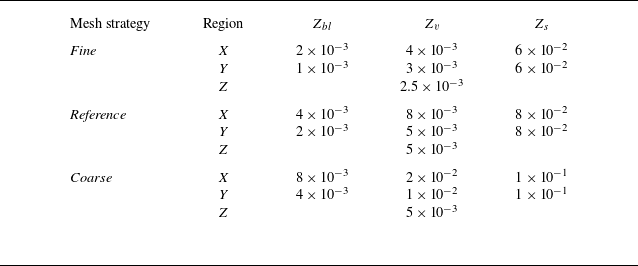


 Open access