
I. INTRODUCTION
Various approaches of statistical learning in the field of machine learning have been extensively studied [Reference Vapnik1, Reference Jebara and Pentland2]. In machine learning, there are two main categories of learning algorithms for building pattern classifiers, namely generative and discriminative training algorithms. In generative training, the probability distribution of data points in each class is estimated using density estimation methods. The parametric modeling approach [Reference Jiang, Hirose and Hou3] is usually adopted to make the density estimation problem more feasible. The parametric modeling is based on an assumption that unknown probability distributions belong to some families of computationally tractable functions, such as the family of exponential distributions [Reference Brown4]. The unknown parameters of the presumed distribution are then estimated from training data using the common maximum-likelihood estimation (MLE) approach. The estimated distributions are then used for pattern classification, such as speech decoding based on the maximum a posteriori (MAP) decision rule. There are many efficient algorithms for training the generative models, such as expectation maximization (EM) [Reference Neal and Hinton5, Reference Dempster, Laird and Rubin6] and Baum–Welch [Reference Baum, Petrie, Soules and Weiss7] algorithms. The advantage of generative training approach is the ability to exploit the inherent dependency among the training data samples. However, the limitation of generative training is the assumption of the distribution of the data set, which is not the actual distribution and accordingly results in a suboptimal performance of the generated classifier.
On the other hand, discriminative training approach does not explicitly attempt to model the data distribution, but instead, it directly optimizes a mapping function from input samples to output labels [Reference He, Deng and Chou8, Reference Jiang9]. Therefore, the discriminative training approach aims to adjust only the decision boundary without constructing a data generator from the entire feature space. In the literature, considerable research effort is applied to discriminative training for improving the speech recognition performance [Reference Valtchev, Odell, Woodland and Young10–Reference Brown16]. The most popular discriminative training criteria include: minimum classification error (MCE) [Reference Juang and Katagiri17–Reference Macherey, Haferkamp, Schlueter and Ney19], maximum mutual information (MMI) [Reference Normandin20–Reference Valtchev, Odell, Woodland and Young22], minimum error rate training (MERT) [Reference Och23], minimum phone/word error (MPE/MWE) [Reference Povey24], and minimum Bayes risk (MBR) [Reference Goel and Byrne25–Reference Gibson and Hain29]. While the MMI method uses mutual information as the criterion for maximization, all other methods attempt to reduce the empirical error by optimizing error rate related objective functions. Although discriminative training is advantageous over generative training in terms of the avoidance of the data distribution assumption imposed on generative training, it has some limitations. For instance, it is not straightforward to exploit the underlying structure of the data in the discriminative models. In automatic speech recognition (ASR) tasks, many pure discriminative models, such as logistic regression, neural networks, and support vector machines (SVM) could not deal with the dynamic nature of speech features [Reference Jiang9]. Hence, to the best of our knowledge, there is no standalone discriminative model gives a comparable performance as the generative models from the perspective of ASR tasks [Reference Jiang9]. However, pure discriminative models can be used as complementary components to generative models.
Recently, generative and discriminative methods are combined into an approach called discriminative training of generative models as an interesting and a new approach in machine learning [Reference Jiang9, Reference Macherey, Haferkamp, Schlueter and Ney19, Reference Jaakkola and Haussler30, Reference Altun, Tsochantaridis and Hofmann31]. This approach is based on including an alternative estimation algorithm for discriminative training rather than the algorithms used for generative modeling. This can be interpreted as a more general framework for using some discriminative criteria that are consistent with the pattern recognition task to learn the generative models. However, state-of-the-art research based on this approach assumes that the acoustic and language models are separate and independent components, and the parameters of these models are usually optimized individually using different criteria [Reference Jiang9, Reference Lin32–Reference Chien and Chueh34]. In that research, several tuning parameters must be well tuned to balance the acoustic and language models scores for the large vocabulary speech recognition (LVCSR) tasks including scaling factor, beam width, and insertion penalty. However, the main drawback of this approach is obvious if we take into consideration the hierarchical matching from phonetic to linguistic levels. In this case, the model-independence assumption becomes unrealistic for obtaining a global optimization of acoustic and language models' parameters.
Motivated by the fact that the acoustic and language models are inherently correlated, this paper proposes a new optimization framework for explicitly training the parameters of acoustic and language models simultaneously using discriminative training. However, to the best of our knowledge, there is a little research in the literature addressing the joint optimization of the parameters of acoustic and language models. What research there is, for example [Reference Lehr and Shafran33, Reference Chien and Chueh34], does not explicitly take into consideration the sentence recognition errors while jointly optimizing the models' parameters. Extending the studies presented in [Reference Juang and Katagiri17, Reference Chou, Lee and Juang35–Reference Kuo, Kingsbury and Zweig41], the focus of the current paper is to propose a new MCE-based discriminative training framework for jointly optimizing parameters of both context-dependent hidden Markov models (HMMs) and n-gram language models on integrated decoding graphs constructed using weighted finite-state transducers (WFSTs). The gain from choosing the MCE as a criterion for the proposed discriminative training framework is the direct minimization of the sentence errors, thus yielding a significant improvement in speech recognition performance after conducting a few training iterations. Additionally, our approach generalizes the MCE discriminant function so as to consider various pronunciations of each word in training utterances while performing the discriminative training.
The main advantage of the proposed framework is the explicit incorporation of the acoustic and language models in the discriminative training procedure, which allows for better consideration of the interdependency between the acoustic and lexical knowledge sources and thus improving the overall recognition performance. On the other hand, the disadvantage of this framework would be the difficulty of fine tuning the training parameters (i.e., leaning rates). However, this disadvantage can be overcome using line search algorithm to look for the best training parameters. We keep this solution in mind to be considered in the future work.
To validate the effectiveness of the proposed approach for jointly optimizing the acoustic and language models, a set of four WFST-based large decoding graphs is constructed to cover a wide range of combinations of these models. These large decoding graphs are composed of two context-dependent HMMs and two n-gram language models to be used throughout our experiments. The primary evaluation presented in this paper, for each task, is the comparison between the MCE-based jointly learnt acoustic and language models and the standard baselines including MLE and MCE-based separately trained acoustic and language models.
This paper is organized as follows. An overview on the MCE-based discriminative training framework is presented in Section II. The joint optimization of the HMM and n-gram parameters is discussed in Section III. The experimental results are then presented and analyzed in Section IV, followed by a summary and discussion in Section V. Finally, the conclusions come in Section VI.
II. MCE-BASED DISCRIMINATIVE TRAINING FRAMEWORK
MCE-based discriminative training is an outcome of a broader class of approaches linked to the design of pattern classifiers referred to as generalized probabilistic descent (GPD)[Reference Katagiri, Lee and Juang12, Reference Katagiri, Lee and Juang36]. The discriminant function for each class in the training set plays an important role in the MCE loss function that represents the core of the MCE-based discriminative training approach. This discriminant function is a smoothed approximation of the score difference between reference and decoding hypotheses and is usually used as a criterion for an objective function [Reference Juang and Katagiri17, Reference McDermott42]. The relation between the true classification risk and the smoothed MCE loss function is recently studied in [Reference Schlueter and Ney43, Reference Ratnagiri, Rabiner and Juang44]. These studies revealed that the direct minimization of the classification error can be achieved if we could minimize the MCE loss function. This makes the MCE-based discriminative training more advantageous than the generative approaches based on learning the probability distribution of data points.
A) Sentence-level discriminant function
The transcription of a speech utterance is usually represented as a sequence of phones or words and is commonly used to formalize the discriminant function of sentence-based MCE [Reference Chou, Lee and Juang35]. The speech signal corresponding to a sentence of words, W, is represented by a sequence of acoustic features, O = (o 1,…,o T ), of length T. The transcription of this signal can be extracted using a cost function, denoted by g(.), which is defined in terms of both log of n-gram probability, log P(W | Γ), where Γ is the n-gram models, and log of HMM probability, log P(O, S |Λ), where Λ is the HMM models and S = (s 1,…,s T ) is the best HMM state sequence of length T [Reference Chou, Lee and Juang35]. This cost function can be written as:
 $$\eqalign{g\lpar O\comma \; W\comma \; \Lambda\comma \; \Gamma\rpar &= \alpha \log P\lpar W \vert \Gamma\rpar + \log P\lpar O\comma \; S \vert \Lambda\rpar \cr &= \alpha \log P\lpar W \vert \Gamma\rpar + \sum_{t = 1}^{T} \log a_{s_{t - 1}} a_{s_{t}}\cr &\quad + \sum_{t = 1}^{T} \log b_{s_{t}}\lpar o_{t}\rpar \comma \; }$$
where α denotes the language model scaling factor and $a_{s_{t-1}s_{t}}$
denotes the state transition probability from HMM state s
t−1 to state s
t
.
$a_{s_{t-1}s_{t}}$
denotes the state transition probability from HMM state s
t−1 to state s
t
. $b_{s_t} \lpar o_t\rpar $
denotes the observation distribution probability of a feature vector o
t
at state s
t
. This distribution is usually modelled as mixtures of Gaussians. Λ denotes HMM parameters (i.e., mixing weights, variances, and means vectors) used to define
$b_{s_t} \lpar o_t\rpar $
denotes the observation distribution probability of a feature vector o
t
at state s
t
. This distribution is usually modelled as mixtures of Gaussians. Λ denotes HMM parameters (i.e., mixing weights, variances, and means vectors) used to define $b_{s_t}\lpar o_t\rpar $
along with the state transition probabilities. Γ refers to the n-gram models including uni-gram, bi-gram, and tri-gram probabilities.
$b_{s_t}\lpar o_t\rpar $
along with the state transition probabilities. Γ refers to the n-gram models including uni-gram, bi-gram, and tri-gram probabilities.
B) Weighted finite-state transducers
To integrate various speech knowledge sources, such as lexical, acoustic, and language models, into a single search space suitable for single-pass decoding, one common choice is WFST [Reference Mohri, Pereira and Riley45–Reference Novak, Minemaysu and Hirose48]. An exciting property of WFST is obvious in its ability to combine these knowledge sources into an elegant and unified recognition network (also called decoding graph). Informally, WFST is a weighted transduction from an input sequence of symbols of one type to an output sequence of symbols of another type. If the inputs and outputs are of the same type, the network is called weighted finite-state acceptor (WFSA). In the current paper, the input symbols are represented by context-dependent acoustic models in the form of tri-phone HMMs, and the output symbols are typically words. The decoding hypotheses are extracted from the WFST using a time synchronous Viterbi beam search algorithm [Reference Hori, Hori and Minami49]. For more details about the WFST (see [Reference Mohri, Pereira and Riley45, Reference Mohri, Pereira and Riley46]).
C) Reference subgraph extraction
To extract a reference subgraph corresponding to each training utterance, two methods can be employed. On the one hand, the authors in [Reference Lin32] presented a method based on inverting the decoding graph then searching for the path carrying the sequence of words equivalent to the transcription of the training utterance. On the other hand, the method presented in [Reference Abdelhamid, Abdulla and MacDonald50] is based on constructing a WFSA corresponding to the reference training utterance, then composing this WFSA with the large decoding graph to extract the reference decoding graph. In this paper, the second method is employed in which a WFSA, A, is constructed to describe the words constituting a training utterance. Then, the constructed WFSA is composed with a large decoding graph, T 1, to generate the reference decoding graph, T 2, using the following composition rule [Reference Allauzen and Schalkwyk51]:
 $$T_2 = \lsqb T_1 \circ A\rsqb \lpar x\comma \; y\rpar = \mathop{\bigoplus}\limits_{x} \lsqb T_1 \lpar x\comma \; y\rpar \rsqb \otimes \lsqb A\lpar y\comma \; y\rpar \rsqb \comma \;$$
where x and y are the input context-dependent phone symbols and the output words, respectively. The symbols ⊕ and ⊗ are the semiring-add and semiring-multiply operations, respectively [Reference Mohri, Pereira and Riley46, Reference Mohri52].
The advantage of this method is that the generated reference WFST usually incorporates all pronunciations of the words of the corresponding training utterance. This allows for better modeling of context-dependent acoustic models, especially when the training corpus contains multiple pronunciations for the same word. After generating the reference-decoding graph, it can be used for decoding the corresponding training speech utterance, resulting in a reference decoding hypothesis. The cost of this reference-decoding hypothesis can be calculated according to equation (1) with respect to the generated reference WFST-based decoding graph T 2 as follows.
 $$g_j \lpar O\comma \; \Lambda\comma \; \Gamma\rpar = \mathop{\max}\limits_{j} g\lpar O\comma \; W_j\comma \; \Lambda\comma \; \Gamma\rpar \comma \;$$
where j is the index of the best reference hypothesis.
D) Discriminant function of the competing hypotheses
To use the MCE criterion, another discriminant function is required, which is corresponding to the cost of the competing hypothesis. This competing hypothesis is usually generated from decoding the speech utterance with respect to the large decoding graph. The discriminant function corresponding to the competing hypotheses can be measured in terms of equation (1) as follows.
 $$g_k \lpar O\comma \; \Lambda\comma \; \Gamma\rpar = \mathop{\max}\limits_{k} g\lpar O\comma \; W_k\comma \; \Lambda\comma \; \Gamma\rpar \comma \;$$
where k is the index of the best competing hypothesis. The general expression of this discriminant function can be defined as follows [Reference Kuo, Lussier, Jiang and Lee53]:
 $$g_k \lpar O\comma \; \Lambda\comma \; \Gamma\rpar = \log \left[{1 \over K} \displaystyle \sum_{k = 1}^{K} e^{g\lpar O\comma W_k\comma \Lambda\comma \Gamma\rpar \eta} \right]^{{1 \over \eta}}\comma \;$$
where K is the number of best competing hypotheses and η is a positive constant used to control the weighting of the best hypotheses. For simplicity, we take into consideration only the topmost competing hypothesis (1-best).
E) Anti-discriminant function
The MCE anti-discriminant function that compares the values of the discriminant functions of the competing hypothesis, k, and the corresponding reference hypothesis, j, is defined as:
 $$d\lpar O\comma \; \Lambda\comma \; \Gamma\rpar = -g_k \lpar O\comma \; \Lambda\comma \; \Gamma\rpar + g_j \lpar O\comma \; \Lambda\comma \; \Gamma \rpar.$$
This measurement can be calculated in terms of either equation (4) or (5). In this paper, we measured the anti-discriminant function in terms of equation (4).
F) Class loss function
In order to use the anti-discriminant function, which is defined in equation (6), in the gradient descent optimization, it is required to be formulated into a smoothed and differentiable 0 − 1 function. One common choice is the sigmoid class loss function which is defined as [Reference Kuo, Lussier, Jiang and Lee53]:
 $$l\lpar O\comma \; \Lambda\comma \; \Gamma\rpar = l\lpar d\lpar O\comma \; \Lambda\comma \; \Gamma\rpar \rpar = l\lpar d\rpar = {1 \over 1+ e^{-\gamma d + \beta}}\comma \;$$
where γ and β are constants used to control the slope and shift of the sigmoid function respectively, and d is the anti-discriminant function defined in equation (6). It is obvious that when the value of the anti-discriminant function d is negative, the loss function will be close to 0. However, it will be close to 1 when the anti-discriminant function is positive. This behavior is controlled by the positive scalar γ. The gradient of the sigmoid class loss function is defined as:
 $$\nabla l\lpar O\comma \; \Lambda\comma \; \Gamma\rpar = \gamma \, l\lpar d\rpar \, \lpar 1- l\lpar d\rpar \rpar.$$
This gradient is used in the derivation of the parameter update formulas based on the GPD algorithm as will be discussed in the next section.
III. OPTIMIZATION METHOD
In this section, we discuss the optimization method used in the proposed training framework for jointly optimizing the acoustic and language models.
A) Gradient decent
The gradient descent method is a general and simple approach that can be applied efficiently to any differential objective function [Reference Wu, Feng and Xu54]. The general form of the gradient descent optimization is represented in terms of an objective function, denoted by F(θ), according to the following iterative update rule along the direction of the gradient.
 $$\theta \lpar n + 1\rpar = \theta \lpar n\rpar - \epsilon \nabla F\lpar \theta\rpar \vert_{\theta = \theta\lpar n\rpar }\comma \;$$
where θ is the model parameters, n is the iteration number, and ε is the training step size, which can be decreased gradually as the iterations proceed in adaptive training [Reference Jiang9]. It is worth noting that, in this paper, the objective function, F(θ), is realized using sigmoid class loss function. Practically, there are two main modes in implementing the above gradient optimization rule, namely batch and online training modes.
On the one hand, the batch mode depends mainly on accumulating the gradient of the model parameters at iteration n for all the training samples, then use this accumulated gradient to update the model parameters, θ(n), only once. The advantage of this method is the possibility of distributing the whole operation on multiple processors. Despite the possibility of parallel processing, the drawback of this method is that it suffers from slow convergence speed due to ignoring the effect of the data correlation in the parameter optimization process.
On the other hand, the online method (also called GPD) is based on updating the model parameters at each iteration after calculating the online gradient for each training sample. The gain from online training is the exploitation of the data correlation, thus accelerating the training process. Since the experiments conducted in the current paper are applied on large vocabulary tasks, we selected the online training to consider the data correlation in the training process and thus accelerating the training convergence.
B) Update equations used in the joint optimization
In this paper, the term joint refers to the acoustic and language models. The acoustic models are usually modeled using statistical HMMs consisting of N states where each state contains Gaussian mixture(s) of K components. The parameter set of a HMM model, Λ, is defined as Λ = {A, c
jk
, U
jk
, R
jk
, where A = [a
sj
] is the state transition matrix, c
jk
is the weight for the k{th} mixture component in the jth state, U
jk
= [μ
jkl
]
l=1
D
is the mean vector and R
jk
is the corresponding covariance matrix which for simplicity, is assumed to be diagonal (i.e., R
k
= [(σ
jkl
)2]
l=1
D
). We also assumed that O = (O
1,…,O
t
,…,O
T
) is a series of feature vectors of length T, where O
t
= (o
t1,…,o
tl
,…,o
tD
) is a feature vector of D dimensions. In the proposed joint optimization framework, we only optimize the Gaussian mixture mean vectors, U
jk
. To maintain the constraints imposed on the mean vectors during the parameter optimization, the following parameter transformation $\lpar \Lambda \rightarrow \tilde{\Lambda}\rpar $
is applied [Reference Juang, Chou and Lee18]:
$\lpar \Lambda \rightarrow \tilde{\Lambda}\rpar $
is applied [Reference Juang, Chou and Lee18]:
 $$\mu_{jkl} \rightarrow \tilde{\mu}_{jkl}\comma \; \quad {\rm where} \quad \tilde{\mu}_{jkl} = {\mu_{jkl} \over \sigma_{jkl}}.$$
In contrast to separate optimization of acoustic and language models [Reference McDermott and Katagiri37, Reference Kuo, Kingsbury and Zweig41, Reference He and Chou55, Reference Lin and Yvon56], we simultaneously optimized the n-gram and HMM parameters. The parameter set of the n-gram model, Γ, is defined as Γ = {β(w
i
), p(w
i
|w
i−1), p(w
i
|w
i−1,w
i−2)}, where β(w
i
) is the back-off probability of the word w
i
, p(w
i
|w
i−1) is the bi-gram probability of the word sequence w
i−1
w
i
, and p(w
i
|w
i−2
w
i−1) is the tri-gram probability of the word sequence w
i−2
w
i−1
w
i
. These n-gram models are integrated with the acoustic models into several decoding graphs using WFSTs. Consequently, the n-gram probabilities are spread over the transitions of the decoding graph. It is worth noting that, the pronunciation model does not have a probabilistic distribution. Therefore, optimizing the transition weights of the decoding graph corresponds to optimizing the n-gram models. Thus, the MCE-based parameter optimization formula of the joint models, $\theta = \lcub \tilde{\Lambda}\comma \; \Gamma \rcub = \lcub \tilde{\mu}_{jkl}\comma \; \Gamma\rcub $
, using the GPD procedure [Reference Katagiri, Lee and Juang12, Reference Katagiri, Lee and Juang36], is defined as:
$\theta = \lcub \tilde{\Lambda}\comma \; \Gamma \rcub = \lcub \tilde{\mu}_{jkl}\comma \; \Gamma\rcub $
, using the GPD procedure [Reference Katagiri, Lee and Juang12, Reference Katagiri, Lee and Juang36], is defined as:
 $$\theta \lpar n+1\rpar = \theta\lpar n\rpar - \epsilon {\partial l_{n}\lpar O\comma \; \Lambda\comma \; \Gamma\rpar \over \partial \theta\lpar n\rpar }\comma \;$$
where n is the training iteration and ε is the training step size. The gradient part of equation (11) can be further written as:
 $$\eqalign{{\partial l_{n}\lpar O\comma \; \Lambda\comma \; \Gamma\rpar \over \partial \theta\lpar n\rpar } &= {\partial l_{n}\lpar O\comma \; \Lambda\comma \; \Gamma\rpar \over \partial d_{n}\lpar O\comma \; \Lambda\comma \; \Gamma\rpar } {\partial d_{n}\lpar O\comma \; \Lambda\comma \; \Gamma\rpar \over \partial \theta\lpar n\rpar } \cr &= \alpha l_{n}\lpar 1-l_{n}\rpar {\partial d_{n}\lpar O\comma \; \Lambda\comma \; \Gamma\rpar \over \partial \theta\lpar n\rpar }.}$$
From equation (12), since $\theta = \lcub \tilde{\Lambda}\comma \; \Gamma\rcub $
, the update rule for optimizing the acoustic model parameters,
$\theta = \lcub \tilde{\Lambda}\comma \; \Gamma\rcub $
, the update rule for optimizing the acoustic model parameters, $\tilde{\Lambda}$
, can be defined as:
$\tilde{\Lambda}$
, can be defined as:
 $$\eqalign{{\partial l_{n}\lpar O\comma \; \Lambda\comma \; \Gamma\rpar \over \partial \tilde{\Lambda}\lpar n\rpar } &= {\partial l_{n}\lpar O\comma \; \Lambda\comma \; \Gamma\rpar \over \partial d_{n}\lpar O\comma \; \Lambda\rpar } {\partial d_{n}\lpar O\comma \; \Lambda\comma \; \Gamma\rpar \over \partial \tilde{\Lambda}\lpar n\rpar }\cr &= \alpha l_{n}\lpar 1 - l_{n}\rpar {\partial d_{n}\lpar O\comma \; \Lambda\comma \; \Gamma\rpar \over \partial \tilde{\Lambda}\lpar n\rpar }.}$$
The update rule for optimizing the Gaussian mean vectors of a HMM can be formulated as the derivative of ${\partial d_{n}\lpar O\comma \; \Lambda\comma \; \Gamma\rpar \over \partial \tilde{\Lambda}\lpar n\rpar }$
with respect to
${\partial d_{n}\lpar O\comma \; \Lambda\comma \; \Gamma\rpar \over \partial \tilde{\Lambda}\lpar n\rpar }$
with respect to $\lcub \tilde{\mu}_{jkl}\rcub $
, which can be written as [Reference Juang, Chou and Lee18]:
$\lcub \tilde{\mu}_{jkl}\rcub $
, which can be written as [Reference Juang, Chou and Lee18]:
 $${\partial d_{n}\lpar O\comma \; \Lambda\comma \; \Gamma\rpar \over \partial \tilde{\mu}_{jkl}\lpar n\rpar } = \sum_{t = 1}^{T} \delta\lpar q_{t} - j\rpar {c_{jk} . b_{jk}\lpar O\rpar \over b_{j}\lpar O\rpar } \left({o_{tl} \over \sigma_{jkl}} - \tilde{\mu}_{jkl} \right)\comma \;$$
where δ(.) is the Kronecker delta function, q t is the state number at time t, and
 $$b_j \lpar O\rpar = \sum_{k = 1}^K c_{j\, k} b_{j\, k} \lpar O\rpar$$
is the observation distribution probability of the speech utterance, O, with respect to Gaussian mixtures at state j, where K is the number of mixture components at the HMM state j, c jk is the mixture weight, and b jk (O) is the probability of the mixture component k, which is defined as:
 $$b_{jk}\lpar O\rpar = {1 \over \sqrt{\left \vert \lpar 2\pi\rpar ^D \Sigma_{jk} \right \vert}} e^{\left(- {1 \over 2} \left(o - \mu_{jk} \right)^{T} \Sigma_{jk}^{-1} \left(o - \mu_{jk} \right)\right)}.$$
Then, using the GPD algorithm, the HMM parameters can be iteratively adjusted using the following update rule:
 $$\lpar \tilde{\Lambda}\rpar _{n+1} = \lpar \tilde{\Lambda}\rpar _{n} - \epsilon_{\Lambda} {\partial l_{n}\lpar O\comma \; \Lambda\comma \; \Gamma\rpar \over \partial \tilde{\Lambda}\lpar n\rpar }\comma \;$$
where εΛ > 0 is a preselected constant used to control the step size of learning the HMM parameters. From equation (17), we can see that the acoustic parameters $\lpar \tilde{\Lambda}\rpar _{n+1}$
at iteration n + 1 are optimized using both the acoustic parameters
$\lpar \tilde{\Lambda}\rpar _{n+1}$
at iteration n + 1 are optimized using both the acoustic parameters $\lpar \tilde{\Lambda}\rpar _{n}$
and the language model parameters Γ (embedded in l
n
(O, Λ, Γ), please refer to equations (7, 6, 3, and 1)) at iteration n. Finally, the inverse transformation is applied to restore the actual updated parameters as follow:
$\lpar \tilde{\Lambda}\rpar _{n}$
and the language model parameters Γ (embedded in l
n
(O, Λ, Γ), please refer to equations (7, 6, 3, and 1)) at iteration n. Finally, the inverse transformation is applied to restore the actual updated parameters as follow:
 $$\lpar \mu_{jkl}\rpar _{n + 1} = \lpar \sigma_{jkl}\rpar _{n} \lpar \tilde{\mu}_{jkl}\rpar _{n + 1}.$$
Back to equation (12), since $\theta = \lcub \tilde{\Lambda}\comma \; \Gamma\rcub $
, the update equation for optimizing the language model parameters can be defined as follows.
$\theta = \lcub \tilde{\Lambda}\comma \; \Gamma\rcub $
, the update equation for optimizing the language model parameters can be defined as follows.
 $$\eqalign{{\partial l_{n}\lpar O\comma \; \Lambda\comma \; \Gamma\rpar \over \partial \Gamma\lpar n\rpar } &= {\partial l_{n}\lpar O\comma \; \Lambda\comma \; \Gamma\rpar \over \partial d_{n}\lpar O\comma \; \Lambda\rpar } {\partial d_{n}\lpar O\comma \; \Lambda\comma \; \Gamma\rpar \over \partial \Gamma\lpar n\rpar }\cr &= \alpha l_{n}\lpar 1 - l_{n}\rpar {\partial d_{n}\lpar O\comma \; \Lambda\comma \; \Gamma\rpar \over \partial \Gamma\lpar n\rpar }.}$$
Viewing the language models Γ as a vector of transition weights, the partial derivative of equation (19) can be defined as [Reference Lin and Yvon56]:
 $${\partial d_{n}\lpar O\comma \; \Lambda\comma \; \Gamma\rpar \over \partial \Gamma\lpar n\rpar } = \left[-I\lpar W_{ref}\comma \; \omega_{n}\rpar + I\lpar W_{best}\comma \; \omega_{n}\rpar \right]\comma \;$$
where I(W ref , ω n ) and I(W best , ω n ) represent the number of occurrences of the transition weight, ω n , at iteration n, in the reference hypothesis W ref and the best competing hypothesis W best , respectively. It is worth noting that, ω n is a scalar value denoting a single transition weight. Then, using the GPD algorithm, the transition weights can be iteratively adjusted using the following update rule:
 $$\omega_{n + 1} = \omega_{n} - \epsilon_{\Gamma} {\partial l_{n}\lpar O\comma \; \Lambda\comma \; \Gamma\rpar \over \partial \Gamma\lpar n\rpar }\comma \;$$
where εΓ > 0 is another preselected constant used to control the step size of learning the graph transition weights. From equation (21), we can see that transition weights ω n+1 are optimized in terms of both the transition weights ω n and the acoustic parameters Λ (embedded in l n (O, Λ, Γ), please see equations (7, 6, 3, and 1)) at iteration n.
C) Training procedure
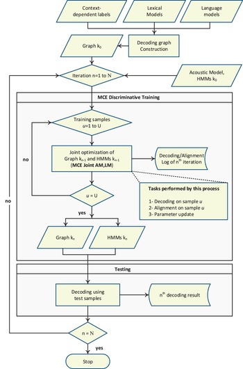
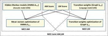
The proposed joint discriminative training framework is shown in Fig. 1. In this framework, both acoustic and language models are optimized simultaneously. Initially, the decoding graph is constructed using a sequence of WFST operations applied using OpenFST toolkit [Reference Allauzen, Riley, Schalkwyk, Skut and Mohri57]. Three knowledge sources, namely lexical, acoustic and language models, are combined to produce a single decoding graphs, called Graph k 0, to be used for further parameter optimization. It is worth noting that, the acoustic models are not included in the WFST operations to reduce the size of the resulting decoding graph. Consequently, the acoustic models are handled separately. Then, all training samples are used to jointly optimize the acoustic and language models' parameters of HMM k 0 and Graph k 0, resulting in another set of acoustic models, HMM k n , and graph, Graph k n , where k denotes the graph number (i.e., 1, 2, 3, and 4), and n is the iteration number (i.e., n = 1, …, N). At each iteration, three steps are performed: decoding, alignment, and parameter update. The result from each step is recorded in a log file for further analysis. On the other hand, in the testing process, the optimized graphs and acoustic models are used in decoding the evaluation sets of TIMIT and Resource Management (RM1). This procedure is performed on each graph, in the set of four decoding graphs, to measure the performance of the jointly optimized parameters.
Flowchart of the proposed joint discriminative training framework for learning the parameters of acoustic and language models on integrated decoding graph. k denotes graph number (i.e., 1, 2, 3, or 4). N and U refer to the number of training iterations and the size of the development set, respectively.
IV. EXPERIMENTS
A) Speech corpora
Two speech corpora, namely TIMIT [Reference Zue, Seneff and Glass58] and RM1 [Reference Price, Fisher, Bernstein and Pallett59], were incorporated in the experiments conducted in this paper.
On the one hand, the TIMIT corpus contains 6300 phonetically rich utterances spoken by 630 speakers, including 438 males and 192 females, from eight dialect regions of American English. Because the size of the TIMIT corpus is not too large (about 4.5 h of audio overall), and because it provides phonetically rich data and expert transcribed time alignments of phonetic units, which are generally not available in other corpora, TIMIT is considered as an excellent test-bed for the initial evaluation of new acoustic modeling techniques. Based on the baseline language models presented in the previous sections, the speech utterances containing out-of-vocabulary (OOV) words were excluded from the experiments. Consequently, the number of utterances of the development set was 4084, and the number of utterances of the evaluation set was 1543 for the complete test set, and 160 for the core test set.
On the other hand, the RM1 corpus consists of a read speech that represents queries about the naval resources. This corpus comprises speaker-independent and speaker-dependent sets of utterances. Only the set of speaker-independent utterances is considered in our experiments. The set of speaker independent utterances consists of 3990 training utterances from 109 speakers, and 1200 test utterances from 12. Similarly, based on the words provided by the vocabularies associated with the previously mentioned language models, the RM1 utterances were filtered to exclude the utterances containing OOV words. Consequently, the number of utterances of the RM1 development set was 2238, and the number of utterances of the RM1 evaluation set was 668.
Table 1 shows the number of training and test utterances of each corpus after removing OOV utterances. Throughout this section, the utterances of the training set are referred to as development set, whereas the utterances of the testing set are referred to as evaluation set.
Number of utterances of the development and evaluation sets of the TIMIT and RM1 speech corpora.
B) Experimental setup
The speech utterances of TIMIT and RM1 were sampled at 16 kHz with 16 bits per sample and framed at a rate of 30 ms with 75% overlap. Each frame is represented by 39-dimensional mel-frequency cepstral coefficients (MFCC) feature vector composed of 12 static coefficients, 24 dynamic coefficients, and 3 log energy values. A set of seed speaker independent acoustic models was estimated from the Wall Street Journal (WSJ) and TIMIT corpora [Reference Vertanen60]. Each acoustic model is represented as a HMM with three states and left-to-right transitions in a linear arrangement without skip transitions. The HMM set employed in this paper is shown in Table 2. This table presents the total number of HMM states (#States), the total number of mixtures per state (#Mix/state) and the number of mean vectors susceptible to optimization.
Baseline acoustic models.
In addition, two sets of n-gram models incorporated in our experiments. These sets are estimated from the Gigawords text corpora based on a vocabulary containing 64K words [Reference Vertanen60]. To reduce the number of n-grams, the baseline language models were pruned using the SRILM toolkit at a threshold of 0.45 × 10⁻⁶ [Reference Stolcke61]. The description of these language models is shown in Table 3, and expressed in terms of the number of uni-grams, bi-grams, and tri-grams along with the perplexity of each set.
Baseline language models.
These sets of acoustic and language models were freely available at [Reference Vertanen62] in the time of writing this paper.
Using the two sets of acoustic and language models, a set of four large WFST-based decoding graphs was constructed to cover a wide range of variations of the HMM and language models' sizes as shown in Table 4. This table shows the various combinations of acoustic and language models used in building the four WFST-based decoding graphs. The size of each decoding graph is also shown and presented in terms of the number of states and transitions along with the memory required to load the full decoding graph. Additionally, Table 5 shows the operations applied to construct Graph1 as an example. In this table, the evolution of the graph size is presented in terms of the number of states and transitions at each step in the construction process.
Baseline large decoding graphs.
Evolution of graph size when constructing the large WFST-based decoding graphs.
C: Context dependency WFST, L: Lexicon WFST, G: n-gram WFST, T: Silence WFST, ∘: Composition operation, det: Determinization operation, ·: Lookahead composition.
The experiments conducted in this section are presented in terms of the following four training approaches based on the MCE-based discriminative training of each decoding graph as shown in Fig. 2.
-
• MCE LM: This approach refers to the separate optimization of the language model parameters on the decoding graphs. In this approach, the acoustic models were kept constant.
-
• MCE AM: This approach refers to the separate optimization of the acoustic models (i.e., HMM mean vectors). In this approach, the language models were kept constant.
-
• (MCE AM, MCE LM): This approach refers to using the resulting models from the previous two approaches in the evaluation process.
-
• (MCE Joint AM, LM): This approach refers to the proposed joint optimization of the acoustic and language models' parameters.
C) Parameter selection
Before experimenting with the GPD procedure we performed a number of experiments aiming at setting the parameters of the class loss function. These parameters include: α that scales the language model scores so that the acoustic and language model scores are balanced in the log-domain; γ that controls the slope of the class loss function; εΛ that controls the step size of learning the acoustic model parameters; and εΓ that controls the step size of learning the language model parameters.
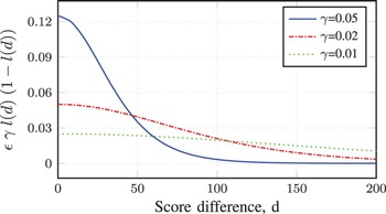
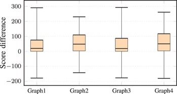
The value of the scaling factor, α, was determined empirically based on the scores of the acoustic and language models. The value of this parameter was selected as 13 for all the experiments conducted in this paper. In addition, the value of γ was determined based on the relationship between the score difference between the reference and competing hypotheses and the value of the parameter adjustment, equation (8). Figure 3 depicts the relationship between the score differences (X-axis) and the value of the parameter adjustment (Y-axis) for three values of γ and a training step size of ε = 10. From this figure, we can see that, the value of the parameter adjustment is large for the score differences less than 80 when taking the value of γ as 0.05. Consequently, the score differences greater than 100 will not significantly contribute to the parameter adjustment. However, when the value of γ was taken as 0.02, the score differences greater than 80 will contribute in the parameter adjustment. Besides, the score difference of the speech utterances of the development set with respect to the four decoding graphs incorporated in the conducted experiments are depicted in Fig. 4. From this figure, we can see that, most of the speech utterances have a score difference between 0 and 120. Therefore, a reasonable selection of the value of γ is 0.02, which take into consideration the score differences greater than 80.
Discriminative training approaches of acoustic and language models' parameters.
Parameter update value (y-axis) for the score differences (x-axis) when ε = 10.
Score difference between reference and competing hypotheses.
Additionally, the values of the training step sizes of the language and acoustic models were determined empirically. One way to select these values is to cut and try based on the following criterion. When the speech corpus in hand is phonetically rich, the step size of learning the acoustic models should be small and vice versa. In our case, the step size of learning the acoustic models was selected in the range from 40 to 100 for the phonetically rich TIMIT corpus, whereas it was selected as a large value in the range from 60 to 150 for the RM1 corpus. Similarly, the step size of learning the language models is selected based on the number of words in the training corpus. If the language models are based on a small vocabulary, then the step size should be selected as small as 2.0. However, the step size of learning the language models based on a larger number of words such as RM1, its value was selected in the range from 1 to 10 based of the order of the language models. The complete set of parameters employed in the experiments conducted in this paper is presented in Table 6. Other parameters that are not listed in this table, their values were set as zero.
Parameter setting for discriminative training and testing.
It has been noted that using the above parameters, the training process converges up to the fifth iteration and becomes constant or diverges afterwards. For this reason, in all experiments, we recorded the evaluation results of the training iterations from the first to the fifth iteration.
D) Performance evaluation
The MCE-based discriminative training was carried out on the MLE baseline models as initial configurations for all the HMMs and n-gram models. For each graph in the set of four decoding graphs, four experiments were conducted. In the first experiment, the acoustic models were trained while fixing the language models. This experiment is dented by MCE AM. Whereas in the second experiment, the language models were trained while fixing the acoustic models. This experiment is denoted by MCE LM. In the third experiment, the resulting graphs from the first two experiments were used in the evaluation process. This third experiment is denoted by (MCE AM, MCE LM). Finally, in the fourth experiment, the acoustic and language models were optimized jointly using the proposed framework. This latter experiment is denoted by (MCE Joint AM,LM). In each experiment, five training iterations of the GPD procedure were employed.
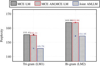
As a gain from the proposed approach, the evolution of the language model perplexity was measured in terms of Graph1 and Graph3 as they are based on tri-gram and bi-gram language models, respectively, as shown in Fig. 5. In this figure, the separate optimization of acoustic and language models (MCE AM, MCE LM), achieved a perplexity similar to that of the language models optimization, MCE LM. However, when using the proposed joint optimization approach (MCE Joint AM/LM), better perplexities were achieved. It is worth noting that, the resulting perplexities are much better than the baseline perplexities which are 375.05 and 411.57 for the tri-gram and bi-gram language models, respectively. These results give an evidence of the appropriateness of the proposed approach to optimally learn the parameters of language models.
Evolution of language model perplexity. The baseline perplexities are 375.05 and 411.57 for the ti-gram (LM1) and bi-gram (LM2) language models, respectively.
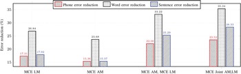
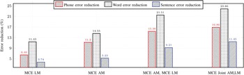
In addition, the percentages of reduction in phone error rate (PER), word error rate (WER), and sentence error rate (SER) are depicted in Figs. 6 and 7 in terms of the evaluation sets of the TIMIT and RM1, respectively. In these figures, the percentages of reduction using the proposed joint optimization approach is better than those of the other approaches, especially the percentage of reductions of the SER, which gives more emphasize on the effectiveness of the proposed approach in handling the correlation between the acoustic and language models.
Error reduction rate (%) using Graph1 on the TIMIT evaluation set with respect to the baseline models.
Error reduction rate (%) using Graph1 on the RM1 evaluation set with respect to the baseline models.
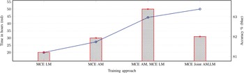
Furthermore, the total time required to learn the models' parameters using the four training approaches, on a machine running at a speed of 2160 MHz with 8 GB memory, is shown in Fig. 8. As shown in this figure, the shortest time is consumed by the training approach MCE LM (as it does not require HMM state sequence alignment), but it achieves less improvement in the word decoding accuracy when compared with the other approaches. In addition, the training using (MCE AM, MCE LM) achieves better decoding accuracy, but it consumes a large training time (sum of the training times of MCE LM and MCE AM approaches). If training of both AM and LM was run in parallel under the (MCE AM, MCE LM) approach, the training time is the same as the time of MCE AM. However, the training using the proposed joint optimization framework consumes a considerably less training time with achieving the highest recognition accuracy. This gives the proposed approach a superiority when compared with the separate optimization approaches.
Average training time and accuracy of four discriminative training approaches.
E) Evaluation of model separation
To further investigate the performance of the joint optimization of both acoustic and language models, the following logarithm of sentence posterior probability of development data, (O, W), was examined [Reference Chien and Chueh34].
 $$\eqalign{\log p\lpar W \vert O\rpar & \approx \log \lsqb p\lpar O \vert W_{ref}\rpar . p\lpar W_{ref}\rpar \rsqb \cr & \quad - \log \lsqb p\lpar O \vert W_{best}\rpar . p\lpar W_{best}\rpar \rsqb .}$$
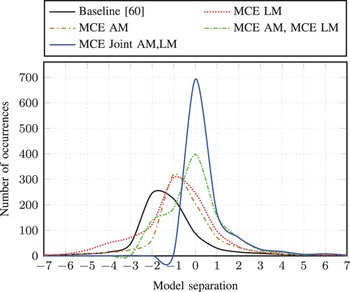
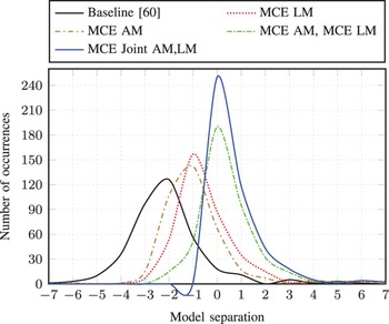
This formula is equivalent to the negative of the misclassification measure explained earlier in this paper, which measures the difference in discriminant function, log p(W, O), between the target hypothesis, W ref , and competing hypothesis, W best . The larger log p(W | O) measured, the bigger model separation between target and competing sentences is obtained. Figure 9 illustrates the histograms of the model separation of the MLE, MCE LM, MCE AM, (MCE AM, MCE LM), and (MCE Joint AM,LM) on the TIMIT complete evaluation set using Graph1. From this figure, we can see that the distribution of (MCE Joint AM,LM) models is shifted right compared with that of all the baselines, and thus yielded an increase in the model separation. Similarly, the histograms of model separation of the MLE, MCE LM, MCE AM, (MCE AM, MCE LM), and (MCE Joint AM, LM) on the RM1 evaluation utterances using Graph1 is also shown in Fig. 10. In this latter figure, the behavior of the model separation is similar to that of the TIMIT evaluation set. Based on these model separations, we can validate the effectiveness of the proposed MCE-based joint optimization approach when compared with the standard separate optimization of acoustic and language models and in terms of the MCE-based discriminative training in benchmark testing of the TIMIT and RM1 speech corpora.
Histogram of model separation calculated by MLE, MCE LM, MCE AM, (MCE AM, MCE LM), and (MCE Joint AM,LM) models on the TIMIT evaluation set using Graph1.
Histogram of model separation calculated by MLE, MCE LM, MCE AM, (MCE AM, MCE LM), and (MCE Joint AM,LM) models on the RM1 evaluation set using Graph1.
V. SUMMARY AND DISCUSSION
For the TIMIT and RM1 continuous speech recognition tasks, significant improvements over all the baselines are obtained as a gain from the proposed (MCE Joint AM, LM) training framework. This emphasizes the effectiveness of the proposed approach on real-world continuous speech recognition tasks. Additional points are analysed and discussed in the following.
-
(1) Advantage: The main advantage of the proposed approach is the improved performance of the jointly optimized acoustic and language models when compared with the separate optimization of these models. This performance was measured in terms of various criteria, such as language model perplexity, decoding error rates, training time, and model separation. For all these criteria, the proposed approach significant improvements.
-
(2) Disadvantage: As the proposed approach incorporates learning the parameters of acoustic and language models jointly, several turning parameters have to be carefully selected, such as learning step size, scaling factor, and slope of the sigmoid function. In this paper, these parameters were empirically selected. Although this is a time consuming method, significant reduction in the training time can be achieved once these parameters are carefully selected. One method to overcome the parameter selection problem is to employee the line search algorithm [Reference Mor'e and Thuente63]. Using this algorithm, the tuning parameters can be dynamically adjusted through the training process, but larger training time is expected.
-
(3) Further improvements: It would be desirable to update the entire HMM and n-gram parameter set using the proposed joint MCE-based training framework. Using the full set additional improvements might be achieved. All results presented in the current paper are achieved from the benchmark testing of the TIMIT and RM1 corpora were based on the 1-best implementation of the MCE discriminant function, corresponding to equation (4) rather than equation (5). However, using more competing hypotheses via either N-best list or word lattice [Reference Schlueter, Macherey, Muller and Ney64] may achieve additional improvements.
VI. CONCLUSION
In this paper, we proposed a new MCE-based discriminative training framework for jointly optimizing the parameters of acoustic and language models on large decoding graphs using the GPD procedure. The effectiveness of the proposed approach, denoted by (MCE Joint AM,LM), was validated in terms of a set of four large WFST-based decoding graphs. The proposed approach achieved significant gains in the speech decoding performance measured in terms of PER, WER, and SER when compared with four baselines; MLE, MCE LM, MCE AM, and (MCE AM, MCE LM) on the four large WFST-based decoding graphs. The language model perplexity has been improved by the MCE LM, (MCE AM, MCE LM), and (MCE Joint AM,LM). However, the percentage of improvement achieved by the proposed approach was larger than the percentage of improvement achieved by the other approaches. In addition, the histograms of model separation showed the superiority of the proposed approach when compared with the separate optimization of the acoustic and language models in benchmark testing of two speech corpora, namely TIMIT and RM1.
ACKNOWLEDGEMENTS
This work is supported by the R&D program of the Korea Ministry of Knowledge and Economy (MKE) and Korea Evaluation Institute of Industrial Technology (KEIT) [KI001836, Development of Mediated Interface Technology for HRI].
Abdelaziz A. Abdelhamid holds a PhD Degree from the University of Auckland, New Zealand. He is a lecturer in the University of Ain Shams, Cairo, Egypt. He was a member of the HealthBots projects sponsored by the University of Auckland and ETRI (Korea). He has published more than 13 publications in international conferences and journals. He received the best paper award from the international conference on social robotics, China. His research interest: Speech recognition, Discriminative training, and Lattice rescoring.
Waleed H. Abdulla holds a PhD Degree from the University of Otago, New Zealand. He is an Associate Professor in the University of Auckland. He was the Vice President- Member Relations and Development (APSIPA) for two terms. He has been a Visiting Researcher/Collaborator with Tsinghua University, Siena University (Italy), Essex University (UK), IDIAP (Switzerland), TIT (Japan), ETRI (Korea), HKPU (Hong Kong). He has published more than 120 refereed publications. He is member of Editorial Boards of six journals. He supervised over 25 postgraduate students. He is a recipient of many awards and funded projects exceeding $1M and was awarded JSPS, ETRI, and Tsinghua fellowships. He received Excellent Teaching Awards for 2005 and 2012. He is a Member of APSIPA and Senior Member of IEEE. His research interest: Human Biometrics, Speech and Signal Processing, and Active Noise Control.


 Open access