


1. Introduction
Over the past few decades, a hydrodynamic-like model has been developed to describe the flow of dry granular matter in open inclined channels. This approach features a generalised version of the Saint-Venant equations for shallow water flow, augmented by the $\mu (I)$
-rheology to account for the special (non-Newtonian) frictional and diffusive properties of granular materials (Forterre & Pouliquen Reference Forterre and Pouliquen2003; GDR-MiDi 2004; Yop et al. Reference Yop, Forterre and Pouliquen2005, Reference Yop, Forterre and Pouliquen2006; Gray & Edwards Reference Gray and Edwards2014; Baker, Barker & Gray Reference Baker, Barker and Gray2016). A number of studies have successfully adopted this approach to capture the dynamics of various waveforms, including travelling and standing waves, erosion-deposition waves and granular avalanches (Forterre Reference Forterre2006; Gray & Cui Reference Gray and Cui2007; Di Cristo et al. Reference Di Cristo, Iervolino, Vacca and Zanuttigh2009; Johnson & Gray Reference Johnson and Gray2011; Gray & Edwards Reference Gray and Edwards2014; Razis et al. Reference Razis, Edwards, Gray and van der Weele2014; Edwards & Gray Reference Edwards and Gray2015; Edwards et al. Reference Edwards, Viroulet, Kokelaar and Gray2017; Viroulet et al. Reference Viroulet, Baker, Edwards, Johnson, Gjaltema, Clavel and Gray2017, Reference Viroulet, Baker, Rocha, Johnson, Kokelaar and Gray2018; Razis, Kanellopoulos & van der Weele Reference Razis, Kanellopoulos and van der Weele2019; Rocha, Johnson & Gray Reference Rocha, Johnson and Gray2019; Russell et al. Reference Russell, Johnson, Edwards, Viroulet and Gray2019; Edwards et al. Reference Edwards, Viroulet, Johnson and Gray2021; Kanellopoulos, Razis & van der Weele Reference Kanellopoulos, Razis and van der Weele2021; Kanellopoulos Reference Kanellopoulos2021; Kanellopoulos, Razis & van der Weele Reference Kanellopoulos, Razis and van der Weele2022; Edwards et al. Reference Edwards, Rocha, Kokelaar, Johnson and Gray2023; Razis, Kanellopoulos & Van der Weele Reference Razis, Kanellopoulos and Van der Weele2023; Kanellopoulos, Razis & van der Weele Reference Kanellopoulos, Razis and van der Weele2024; Kanellopoulos Reference Kanellopoulos2025). One waveform, however, has remained relatively unexplored: the solitary wave. To the best of our knowledge, it is an open question whether flowing granular sheets can sustain such a wave. Hitherto, solitary granular waves have been reported in theoretical studies by Razis et al. (Reference Razis, Kanellopoulos and van der Weele2019) (see especially figure 8c therein) and Kanellopoulos et al. (Reference Kanellopoulos, Razis and van der Weele2022) (see figure 9 therein), but these waves required an unrealistic amount of fine tuning of the system parameters and, in addition, their stability was questionable. In this paper, we follow a different route and the solitary waves in question are sufficiently robust to make their detection in experiments feasible: we establish the conditions under which a localised perturbation of the flow gives rise to one single roll wave. Usually, this type of perturbation generates a whole group of roll waves. By tuning the system parameters, however, the formation of all but the first roll wave can be suppressed for arbitrarily long times. This means that – on any chute of finite length – the leading roll wave will remain solitary.
$\mu (I)$
-rheology to account for the special (non-Newtonian) frictional and diffusive properties of granular materials (Forterre & Pouliquen Reference Forterre and Pouliquen2003; GDR-MiDi 2004; Yop et al. Reference Yop, Forterre and Pouliquen2005, Reference Yop, Forterre and Pouliquen2006; Gray & Edwards Reference Gray and Edwards2014; Baker, Barker & Gray Reference Baker, Barker and Gray2016). A number of studies have successfully adopted this approach to capture the dynamics of various waveforms, including travelling and standing waves, erosion-deposition waves and granular avalanches (Forterre Reference Forterre2006; Gray & Cui Reference Gray and Cui2007; Di Cristo et al. Reference Di Cristo, Iervolino, Vacca and Zanuttigh2009; Johnson & Gray Reference Johnson and Gray2011; Gray & Edwards Reference Gray and Edwards2014; Razis et al. Reference Razis, Edwards, Gray and van der Weele2014; Edwards & Gray Reference Edwards and Gray2015; Edwards et al. Reference Edwards, Viroulet, Kokelaar and Gray2017; Viroulet et al. Reference Viroulet, Baker, Edwards, Johnson, Gjaltema, Clavel and Gray2017, Reference Viroulet, Baker, Rocha, Johnson, Kokelaar and Gray2018; Razis, Kanellopoulos & van der Weele Reference Razis, Kanellopoulos and van der Weele2019; Rocha, Johnson & Gray Reference Rocha, Johnson and Gray2019; Russell et al. Reference Russell, Johnson, Edwards, Viroulet and Gray2019; Edwards et al. Reference Edwards, Viroulet, Johnson and Gray2021; Kanellopoulos, Razis & van der Weele Reference Kanellopoulos, Razis and van der Weele2021; Kanellopoulos Reference Kanellopoulos2021; Kanellopoulos, Razis & van der Weele Reference Kanellopoulos, Razis and van der Weele2022; Edwards et al. Reference Edwards, Rocha, Kokelaar, Johnson and Gray2023; Razis, Kanellopoulos & Van der Weele Reference Razis, Kanellopoulos and Van der Weele2023; Kanellopoulos, Razis & van der Weele Reference Kanellopoulos, Razis and van der Weele2024; Kanellopoulos Reference Kanellopoulos2025). One waveform, however, has remained relatively unexplored: the solitary wave. To the best of our knowledge, it is an open question whether flowing granular sheets can sustain such a wave. Hitherto, solitary granular waves have been reported in theoretical studies by Razis et al. (Reference Razis, Kanellopoulos and van der Weele2019) (see especially figure 8c therein) and Kanellopoulos et al. (Reference Kanellopoulos, Razis and van der Weele2022) (see figure 9 therein), but these waves required an unrealistic amount of fine tuning of the system parameters and, in addition, their stability was questionable. In this paper, we follow a different route and the solitary waves in question are sufficiently robust to make their detection in experiments feasible: we establish the conditions under which a localised perturbation of the flow gives rise to one single roll wave. Usually, this type of perturbation generates a whole group of roll waves. By tuning the system parameters, however, the formation of all but the first roll wave can be suppressed for arbitrarily long times. This means that – on any chute of finite length – the leading roll wave will remain solitary.
(a) A periodic train of fully ripened granular roll waves, propagating with speed $c$
along a chute inclined at an angle
$c$
along a chute inclined at an angle $\zeta$
. Roll waves are the dominant travelling waveform when the Froude number
$\zeta$
. Roll waves are the dominant travelling waveform when the Froude number ${\textit{Fr}}$
exceeds a critical value
${\textit{Fr}}$
exceeds a critical value $ {\textit{Fr}}_{cr}$
as defined by (2.6). To highlight the typical shape of the roll waves, only the upper part of the granular sheet (close to the free surface) has been depicted and the vertical scale has been greatly expanded. In reality, the wavelength of these waves is much larger than the height of the sheet, which in turn is significantly larger than the wave amplitude. (b) Successive stages in the development of a group of roll waves caused by a localised initial perturbation (blue) at the top of the chute. For economy of space, here – and in all figures to follow – the chute has been depicted horizontally with the understanding that it is actually tilted by an angle
$ {\textit{Fr}}_{cr}$
as defined by (2.6). To highlight the typical shape of the roll waves, only the upper part of the granular sheet (close to the free surface) has been depicted and the vertical scale has been greatly expanded. In reality, the wavelength of these waves is much larger than the height of the sheet, which in turn is significantly larger than the wave amplitude. (b) Successive stages in the development of a group of roll waves caused by a localised initial perturbation (blue) at the top of the chute. For economy of space, here – and in all figures to follow – the chute has been depicted horizontally with the understanding that it is actually tilted by an angle $\zeta$
.
$\zeta$
.

Roll waves form spontaneously when the Froude number ${\textit{Fr}}$
of the incoming flow at the top of the chute exceeds a certain critical value
${\textit{Fr}}$
of the incoming flow at the top of the chute exceeds a certain critical value ${\textit{Fr}}_{cr}$
(to be specified in § 2). Beyond this threshold, the uniform flow is unstable. Small perturbations on the surface of the flowing sheet are amplified and grow, given time, into a periodic train of roll waves (Savage & Hutter Reference Savage and Hutter1989; Forterre & Pouliquen Reference Forterre and Pouliquen2003; Gray & Edwards Reference Gray and Edwards2014; Razis et al. Reference Razis, Edwards, Gray and van der Weele2014; Edwards & Gray Reference Edwards and Gray2015; Razis et al. Reference Razis, Kanellopoulos and van der Weele2019; Fei et al. Reference Fei, Jie, Xiong and Wu2021; Kanellopoulos et al. Reference Kanellopoulos, Razis and van der Weele2022; Razis et al. Reference Razis, Kanellopoulos and Van der Weele2023). The formation of such a train, however, is a multi-step procedure in which the larger (and therefore faster) travelling perturbations overtake the smaller (and thus slower) ones. In this way, the larger perturbations grow at the expense of the smaller ones, and begin to resemble roll waves with their characteristic steep front and long, gradually diminishing tail. This coarsening process continues – if the chute is long enough – until the waves reach equal size, at which point the coarsening is arrested, as described by Razis et al. (Reference Razis, Edwards, Gray and van der Weele2014). Figure 1(a) shows such a fully ripened roll wave train.
${\textit{Fr}}_{cr}$
(to be specified in § 2). Beyond this threshold, the uniform flow is unstable. Small perturbations on the surface of the flowing sheet are amplified and grow, given time, into a periodic train of roll waves (Savage & Hutter Reference Savage and Hutter1989; Forterre & Pouliquen Reference Forterre and Pouliquen2003; Gray & Edwards Reference Gray and Edwards2014; Razis et al. Reference Razis, Edwards, Gray and van der Weele2014; Edwards & Gray Reference Edwards and Gray2015; Razis et al. Reference Razis, Kanellopoulos and van der Weele2019; Fei et al. Reference Fei, Jie, Xiong and Wu2021; Kanellopoulos et al. Reference Kanellopoulos, Razis and van der Weele2022; Razis et al. Reference Razis, Kanellopoulos and Van der Weele2023). The formation of such a train, however, is a multi-step procedure in which the larger (and therefore faster) travelling perturbations overtake the smaller (and thus slower) ones. In this way, the larger perturbations grow at the expense of the smaller ones, and begin to resemble roll waves with their characteristic steep front and long, gradually diminishing tail. This coarsening process continues – if the chute is long enough – until the waves reach equal size, at which point the coarsening is arrested, as described by Razis et al. (Reference Razis, Edwards, Gray and van der Weele2014). Figure 1(a) shows such a fully ripened roll wave train.
The above-mentioned scenario holds when the roll waves are allowed to develop spontaneously from the naturally occurring tiny perturbations (on the surface of the uniform flow) along the entire length of the channel. One may also generate roll waves by expressly introducing not-so-tiny disturbances at the top of the chute, e.g. by repeatedly raising and lowering the inlet for a short time interval. This is a technique that was used by Brock (Reference Brock1967) and more recently by Yu & Chu (Reference Yu and Chu2022) to create roll waves in a water channel. These authors found that the disturbance at the inlet of the channel first generates a series of well-separated roll waves consisting of an exceptionally large front runner and several trailing waves of successively smaller amplitude and wavelength; see figure 1(b) for a similar observation in the granular flow studied in the present paper. In the wake of this initial series of waves, when the amplitude and wavelength have fallen to their final values, the standard periodic train of roll waves establishes itself (Yu & Chu Reference Yu and Chu2022).
Here, we employ the same method to generate roll waves on a chute with granular matter, and moreover, we specify the conditions under which the second and subsequent waves are suppressed to such a degree that the front runner will effectively travel alone. It will exit the end of any finite chute before the second wave is generated and, in this way, the front runner manifests itself as the sought-after granular solitary wave.
The paper is organised as follows. In § 2, the governing equations are given, being the generalised Saint-Venant equations for granular channel flow, together with the closure relations for the friction exerted by the chute on the flowing material and for the diffusive forces arising from the in-plane stresses within the sheet. Here, we also present the non-dimensional formulation of the model and the numerical scheme used to solve the equations. Section 3 then describes in detail how the granular solitary wave is produced and we show that its wave speed is in good agreement with the analytical prediction by Razis et al. (Reference Razis, Edwards, Gray and van der Weele2014). Section 4 discusses the effect of varying the system parameters, providing a road map for generating such a wave in actual experiment. Finally, § 5 summarises our results.
2. Governing equations
2.1. Generalised Saint-Venant equations for granular flow
The fact that the wavelength of the roll waves is much larger than the height of the sheet, which in turn is significantly larger than the amplitude of the waves (see the caption of figure 1), justifies the use of an analysis similar to the shallow water approximation for open channel flow. The relevant quantities for this approach are the sheet’s height, $h(x,t)$
, and the average velocity,
$h(x,t)$
, and the average velocity, $\bar u(x,t)$
, defined as
$\bar u(x,t)$
, defined as
 \begin{equation} \bar u(x,t) = \frac {1}{h(x,t)}\int _{0}^{h(x,t)} u(x,z,t) \,\textrm{d}z, \end{equation}
where $u(x,z,t)$
is the detailed velocity profile along the vertical cross-section of the sheet. Any variations in the
$u(x,z,t)$
is the detailed velocity profile along the vertical cross-section of the sheet. Any variations in the $y$
-direction (from side to side of the channel) are ignored.
$y$
-direction (from side to side of the channel) are ignored.
The dynamics of the sheet can then be described by two coupled, nonlinear partial differential equations governing $h(x,t)$
and
$h(x,t)$
and $\bar u(x,t)$
(Gray & Edwards Reference Gray and Edwards2014; Razis et al. Reference Razis, Edwards, Gray and van der Weele2014; Edwards & Gray Reference Edwards and Gray2015; Edwards et al. Reference Edwards, Viroulet, Kokelaar and Gray2017; Razis et al. Reference Razis, Kanellopoulos and van der Weele2018, Reference Razis, Kanellopoulos and van der Weele2019):
$\bar u(x,t)$
(Gray & Edwards Reference Gray and Edwards2014; Razis et al. Reference Razis, Edwards, Gray and van der Weele2014; Edwards & Gray Reference Edwards and Gray2015; Edwards et al. Reference Edwards, Viroulet, Kokelaar and Gray2017; Razis et al. Reference Razis, Kanellopoulos and van der Weele2018, Reference Razis, Kanellopoulos and van der Weele2019):
 \begin{align}&\qquad\qquad\qquad\qquad\qquad\qquad\quad \frac {\partial h}{\partial t} + \frac {\partial }{\partial x} (h \bar u) = 0, \end{align}
 \begin{align}& \frac {\partial }{\partial t} (h \bar u) + \frac {\partial }{\partial x} (h \bar {u}^2) = gh\sin \zeta - \frac {\partial }{\partial x}\!\left (\!\frac {1}{2}gh^2\cos \zeta \!\right )\! - \mu (h, \bar {u})gh \cos \zeta \!+ \!\frac {\partial }{\partial x}\!\left (\!\nu (\zeta ) h^{3/2}\frac {\partial \bar u}{\partial x}\!\right )\!, \end{align}
which represent the mass conservation within the sheet and the momentum balance, respectively. Here, it should be noted that, following the approach of Savage & Hutter (Reference Savage and Hutter1989), the granular material is treated as an incompressible fluid, with a constant density that has been divided out of equations (2.2) and (2.3). The equations also reflect the fact that we confine our attention to the $(x,z)$
-plane and that any transport in the cross-wise direction is neglected.
$(x,z)$
-plane and that any transport in the cross-wise direction is neglected.
The left-hand side of (2.3) expresses the rate of change (i.e. the Stokesian derivative) of the depth-averaged momentum. The right-hand side contains the various forces integrated across the sheet’s depth. In order of appearance: (i) the gravitational component acting in the direction of the flow ( $x$
-direction); (ii) the pressure gradient arising from variations in the sheet’s height
$x$
-direction); (ii) the pressure gradient arising from variations in the sheet’s height $h(x,t)$
; (iii) the frictional resistance exerted by the chute’s surface, modelled by a friction coefficient
$h(x,t)$
; (iii) the frictional resistance exerted by the chute’s surface, modelled by a friction coefficient $\mu (h, \bar {u})$
(which depends on both height and velocity) multiplied by the normal force acting on the sheet; and finally, (iv) a diffusive term accounting for the net effect of the in-plane stresses within the sheet, averaged across its depth, which overall behaves very much like a viscous force despite its nonlinear form and the fact that
$\mu (h, \bar {u})$
(which depends on both height and velocity) multiplied by the normal force acting on the sheet; and finally, (iv) a diffusive term accounting for the net effect of the in-plane stresses within the sheet, averaged across its depth, which overall behaves very much like a viscous force despite its nonlinear form and the fact that $\nu (\zeta )$
is expressed in m
$\nu (\zeta )$
is expressed in m $^{3/2}$
s
$^{3/2}$
s $^{-1}$
, which is different from the usual dimensions (m
$^{-1}$
, which is different from the usual dimensions (m $^2$
s
$^2$
s $^{-1}$
) of a viscosity coefficient. Both
$^{-1}$
) of a viscosity coefficient. Both $\mu (h,\bar {u})$
and
$\mu (h,\bar {u})$
and $\nu (\zeta )$
, which account for the specific frictional and diffusive characteristics of granular materials, are derived on the grounds of what is now known as the
$\nu (\zeta )$
, which account for the specific frictional and diffusive characteristics of granular materials, are derived on the grounds of what is now known as the $\mu (I)$
-rheology (Pouliquen & Forterre Reference Pouliquen and Forterre2002; GDR-MiDi 2004).
$\mu (I)$
-rheology (Pouliquen & Forterre Reference Pouliquen and Forterre2002; GDR-MiDi 2004).
Regarding the friction coefficient $\mu (h,\bar {u})$
, we use the following expression from Edwards et al. (Reference Edwards, Viroulet, Kokelaar and Gray2017):
$\mu (h,\bar {u})$
, we use the following expression from Edwards et al. (Reference Edwards, Viroulet, Kokelaar and Gray2017):
 \begin{equation} \mu (h,\bar u) = \tan \zeta _1 + (\tan \zeta _2 - \tan \zeta _1)\left (1 + \frac {\beta h}{\mathcal{L} ({\textit{Fr}}+\varGamma )}\right )^{-1}\!, \end{equation}
where $\zeta _1$
,
$\zeta _1$
, $\zeta _2$
,
$\zeta _2$
, $\mathcal{L}$
,
$\mathcal{L}$
, $\beta$
and
$\beta$
and $\varGamma$
are experimentally determined parameters, and
$\varGamma$
are experimentally determined parameters, and ${\textit{Fr}}$
is the Froude number of the flow.
${\textit{Fr}}$
is the Froude number of the flow.
The inclination angles $\zeta _{1}$
and
$\zeta _{1}$
and $\zeta _{2}$
define the bounds between which the chute can sustain a uniform flow. If the inclination angle of the chute (
$\zeta _{2}$
define the bounds between which the chute can sustain a uniform flow. If the inclination angle of the chute ( $\zeta$
) is less than
$\zeta$
) is less than $\zeta _{1}$
, the granular sheet remains immobile. Conversely, if
$\zeta _{1}$
, the granular sheet remains immobile. Conversely, if $\zeta$
is larger than
$\zeta$
is larger than $\zeta _{2}$
, the sheet avalanches downwards in an accelerated fashion.
$\zeta _{2}$
, the sheet avalanches downwards in an accelerated fashion.
The length scale $\mathcal{L}$
is an experimental fit parameter, typically of the order of a few particle diameters (Pouliquen & Forterre Reference Pouliquen and Forterre2002; Edwards et al. Reference Edwards, Viroulet, Kokelaar and Gray2017). The parameters
$\mathcal{L}$
is an experimental fit parameter, typically of the order of a few particle diameters (Pouliquen & Forterre Reference Pouliquen and Forterre2002; Edwards et al. Reference Edwards, Viroulet, Kokelaar and Gray2017). The parameters $\beta$
and
$\beta$
and $\varGamma$
are dimensionless constants introduced to make (2.4) amendable to the measured data for a variety of materials. The constant
$\varGamma$
are dimensionless constants introduced to make (2.4) amendable to the measured data for a variety of materials. The constant $\varGamma$
represents an offset of the Froude number, making the friction law also applicable to the flow of rough particles. The precise values of
$\varGamma$
represents an offset of the Froude number, making the friction law also applicable to the flow of rough particles. The precise values of $\mathcal{L}$
,
$\mathcal{L}$
, $\beta$
and
$\beta$
and $\varGamma$
depend on the physical properties of the granular material used as well as on the roughness of the underlying surface.
$\varGamma$
depend on the physical properties of the granular material used as well as on the roughness of the underlying surface.
Edwards et al. (Reference Edwards, Viroulet, Kokelaar and Gray2017) introduced an additional parameter $\beta _{*}$
, being the Froude number of the thinnest possible uniform flow. The latter is determined experimentally by measuring the thickness of the residual layer which is left on the chute after the supply at the inlet has been turned off and the surplus of granular material has been allowed to flow out of the system. The specific values of
$\beta _{*}$
, being the Froude number of the thinnest possible uniform flow. The latter is determined experimentally by measuring the thickness of the residual layer which is left on the chute after the supply at the inlet has been turned off and the surplus of granular material has been allowed to flow out of the system. The specific values of $\beta _{*}$
given in table 1 have been taken from the relevant publications by Russell et al. (Reference Russell, Johnson, Edwards, Viroulet and Gray2019) for glass beads, Edwards et al. (Reference Edwards, Russell, Johnson and Gray2019) for carborundum particles and Edwards et al. (Reference Edwards, Rocha, Kokelaar, Johnson and Gray2023) for fine sand.
$\beta _{*}$
given in table 1 have been taken from the relevant publications by Russell et al. (Reference Russell, Johnson, Edwards, Viroulet and Gray2019) for glass beads, Edwards et al. (Reference Edwards, Russell, Johnson and Gray2019) for carborundum particles and Edwards et al. (Reference Edwards, Rocha, Kokelaar, Johnson and Gray2023) for fine sand.
Experimentally obtained parameter values used in the numerical simulations, concerning the flow of three different materials over channels with glass beads glued to the bottom: (i) glass beads (Russell et al. Reference Russell, Johnson, Edwards, Viroulet and Gray2019); (ii) carborundum particles (Edwards et al. Reference Edwards, Russell, Johnson and Gray2019); and (iii) fine sand (Edwards et al. Reference Edwards, Rocha, Kokelaar, Johnson and Gray2023). The symbol $d$
signifies the (mean) particle diameter. In all simulations, we use
$d$
signifies the (mean) particle diameter. In all simulations, we use $g=9.81$
m s
$g=9.81$
m s $^{-2}$
.
$^{-2}$
.

As long as ${\textit{Fr}}(x,t) \geqslant \beta _{*}$
everywhere along the chute, the granular flow will remain fully dynamic (Edwards et al. Reference Edwards, Viroulet, Kokelaar and Gray2017), with the Froude number
${\textit{Fr}}(x,t) \geqslant \beta _{*}$
everywhere along the chute, the granular flow will remain fully dynamic (Edwards et al. Reference Edwards, Viroulet, Kokelaar and Gray2017), with the Froude number ${\textit{Fr}}(x,t)$
being defined as
${\textit{Fr}}(x,t)$
being defined as
 \begin{equation} {\textit{Fr}}(x,t)\,=\,\frac {\bar u(x,t)}{ \sqrt { h(x,t) g \cos \zeta } } . \end{equation}
Also, for ${\textit{Fr}} \geqslant {\textit{Fr}}_{cr}$
, the uniform flow becomes unstable and gives way to roll waves, where the critical Froude number is given by (Forterre & Pouliquen Reference Forterre and Pouliquen2003; Kanellopoulos Reference Kanellopoulos2021)
${\textit{Fr}} \geqslant {\textit{Fr}}_{cr}$
, the uniform flow becomes unstable and gives way to roll waves, where the critical Froude number is given by (Forterre & Pouliquen Reference Forterre and Pouliquen2003; Kanellopoulos Reference Kanellopoulos2021)
 \begin{equation} {\textit{Fr}}_{cr}\,=\,\frac {2}{3} \left ( 1 - \varGamma \right )\!, \end{equation}
which depends only on the aforementioned Froude offset $\varGamma$
. So, to generate roll waves, one has to ensure that the Froude number exceeds both
$\varGamma$
. So, to generate roll waves, one has to ensure that the Froude number exceeds both $\beta _{*}$
and
$\beta _{*}$
and ${\textit{Fr}}_{cr}$
, i.e.
${\textit{Fr}}_{cr}$
, i.e. ${\textit{Fr}}(x,t) \gt {\textit{max}}(\beta _{*}, {\textit{Fr}}_{cr})$
.
${\textit{Fr}}(x,t) \gt {\textit{max}}(\beta _{*}, {\textit{Fr}}_{cr})$
.
Coefficient $\nu (\zeta )$
of the diffusive term in (2.3) as a function of
$\nu (\zeta )$
of the diffusive term in (2.3) as a function of $\zeta$
, see (2.7). The regions outside the interval
$\zeta$
, see (2.7). The regions outside the interval $\zeta _1 \lt \zeta \lt \zeta _2$
are shaded to indicate that the
$\zeta _1 \lt \zeta \lt \zeta _2$
are shaded to indicate that the $\mu (I)$
-rheology on which the evaluation of
$\mu (I)$
-rheology on which the evaluation of $\nu (\zeta )$
is based becomes ill-posed there. For the construction of this plot, the numerical values of the parameters featuring in
$\nu (\zeta )$
is based becomes ill-posed there. For the construction of this plot, the numerical values of the parameters featuring in $\nu (\zeta )$
are those of table 1, set (iii). The parameter sets (i) and (ii) yield qualitatively similar plots.
$\nu (\zeta )$
are those of table 1, set (iii). The parameter sets (i) and (ii) yield qualitatively similar plots.

Regarding the second key parameter in the momentum balance (2.3), the coefficient $\nu (\zeta )$
of the diffusive term, we employ the analytic expression derived by Gray & Edwards (Reference Gray and Edwards2014) building upon earlier work by Forterre (Reference Forterre2006):
$\nu (\zeta )$
of the diffusive term, we employ the analytic expression derived by Gray & Edwards (Reference Gray and Edwards2014) building upon earlier work by Forterre (Reference Forterre2006):
 \begin{equation} \nu (\zeta ) = \frac {2 \mathcal{L} \sqrt {g} \sin \zeta }{9 \beta \sqrt {\cos \zeta }}\,\gamma (\zeta ),\quad \textrm {where}\; \gamma (\zeta ) = \frac {\tan \zeta _2 - \tan \zeta }{\tan \zeta - \tan \zeta _1}. \end{equation}
This coefficient $\nu (\zeta )$
, which will play an important role in our method for generating solitary waves, is depicted in figure 2. It should be noted that (2.7) is only valid within the range of inclination angles where steady uniform flows are possible, i.e. for
$\nu (\zeta )$
, which will play an important role in our method for generating solitary waves, is depicted in figure 2. It should be noted that (2.7) is only valid within the range of inclination angles where steady uniform flows are possible, i.e. for $\zeta _1 \lt \zeta \lt \zeta _2$
. Outside this range, (2.7) takes on negative values and the diffusive term would no longer act as a levelling mechanism, but rather as a term that would enhance the height differences in the sheet; this can be attributed to the ill-posedness of the
$\zeta _1 \lt \zeta \lt \zeta _2$
. Outside this range, (2.7) takes on negative values and the diffusive term would no longer act as a levelling mechanism, but rather as a term that would enhance the height differences in the sheet; this can be attributed to the ill-posedness of the $\mu (I)$
-rheology below
$\mu (I)$
-rheology below $\zeta _1$
and above
$\zeta _1$
and above $\zeta _2$
. At the lower critical angle (
$\zeta _2$
. At the lower critical angle ( $\zeta = \zeta _1$
), the value of
$\zeta = \zeta _1$
), the value of $\nu (\zeta )$
approaches infinity, while at the upper critical angle (
$\nu (\zeta )$
approaches infinity, while at the upper critical angle ( $\zeta = \zeta _2$
), it becomes zero.
$\zeta = \zeta _2$
), it becomes zero.
To conclude this section, we note that under uniform flow conditions, i.e. $h(x,t)=h_0$
and
$h(x,t)=h_0$
and $\bar {u}(x,t)=\bar {u}_0$
, the mass balance (2.2) is trivially satisfied and the momentum balance (2.3) reduces to
$\bar {u}(x,t)=\bar {u}_0$
, the mass balance (2.2) is trivially satisfied and the momentum balance (2.3) reduces to $\tan \zeta =\mu (h_0,\bar u_0)$
. This implies (Kanellopoulos Reference Kanellopoulos2021)
$\tan \zeta =\mu (h_0,\bar u_0)$
. This implies (Kanellopoulos Reference Kanellopoulos2021)
 \begin{equation} h_0 = \frac {\mathcal{L} \gamma (\zeta )}{\beta }\,({\textit{Fr}}_0+\varGamma ), \quad \bar {u}_0 = \frac {\beta \sqrt {g \cos \zeta }}{\mathcal{L} \gamma (\zeta )}\,h_{0}^{3/2} - \varGamma \sqrt {g \cos \zeta }\, h_{0}^{1/2}, \end{equation}
where ${\textit{Fr}}_0$
is the Froude number of the uniform flow in question. This will be the base flow on which we will impose the local perturbation at the inlet to generate roll waves.
${\textit{Fr}}_0$
is the Froude number of the uniform flow in question. This will be the base flow on which we will impose the local perturbation at the inlet to generate roll waves.
2.2. Non-dimensional formulation
The model for granular flow presented in the previous subsection can be cast in non-dimensional form by expressing all length scales (both the position $x$
along the chute and the height
$x$
along the chute and the height $h(x,t)$
of the sheet) in terms of the thickness
$h(x,t)$
of the sheet) in terms of the thickness $h_0$
of the uniform base flow. A natural choice for the unit of time then is
$h_0$
of the uniform base flow. A natural choice for the unit of time then is $h_0/\bar {u}_0$
, so the non-dimensional variables become
$h_0/\bar {u}_0$
, so the non-dimensional variables become $\tilde {x}= x /h_{0}$
and
$\tilde {x}= x /h_{0}$
and $ \tilde {t} = t / (h_{0}/\bar {u}_{0})$
, where tildes denote non-dimensional quantities. The height and depth-averaged velocity are thus rescaled as follows:
$ \tilde {t} = t / (h_{0}/\bar {u}_{0})$
, where tildes denote non-dimensional quantities. The height and depth-averaged velocity are thus rescaled as follows:
 \begin{equation} \tilde {h}= \frac {h}{h_{0}},\quad \tilde {\bar u}=\frac {\bar {u}}{\bar {u}_{0}}. \end{equation}
The mass balance (2.2) proves to be invariant for this transformation and now reads
 \begin{equation} \frac {\partial \tilde {h}}{\partial \tilde {t}} + \frac {\partial }{\partial \tilde {x}} (\tilde {h} \tilde {\bar u}) = 0, \end{equation}
whereas the momentum balance (2.3) takes the following form (Kanellopoulos et al. Reference Kanellopoulos, Razis and van der Weele2022):
 \begin{equation} {\textit{Fr}}_{0}^2 \left (\frac {\partial }{\partial \tilde {t}} (\tilde {h} \tilde {\bar u}) + \frac {\partial }{\partial \tilde {x}} (\tilde {h} \tilde {\bar {u}}^2)\right ) = \tilde {h}\big (\!\tan \zeta -\mu (\tilde {h},\tilde {u})\big )- \tilde {h}\frac {\partial \tilde {h}}{\partial \tilde {x}} + \frac {{\textit{Fr}}_{0}^2}{R_0}\frac {\partial }{\partial \tilde {x}}\left (\tilde {h}^{3/2}\frac {\partial \tilde {\bar u}}{\partial \tilde {x}}\right )\!, \end{equation}
where ${\textit{Fr}}_0$
is the Froude number of the uniform base flow and
${\textit{Fr}}_0$
is the Froude number of the uniform base flow and $ {R}_0$
is the granular analogue of the Reynolds number introduced by Gray & Edwards (Reference Gray and Edwards2014), again defined in terms of the base flow quantities:
$ {R}_0$
is the granular analogue of the Reynolds number introduced by Gray & Edwards (Reference Gray and Edwards2014), again defined in terms of the base flow quantities:
 \begin{equation} {R}_0=\frac {\bar u_{0}\sqrt {h_{0}}}{\nu (\zeta )}. \end{equation}
Naturally, also the friction coefficient $\mu$
must, in this context, be expressed as a function of the new dimensionless parameters:
$\mu$
must, in this context, be expressed as a function of the new dimensionless parameters:
 \begin{equation} \mu (\tilde {h},\tilde {\bar u}) = \tan \zeta _1 + (\tan \zeta _2 - \tan \zeta _1)\left (1 + \frac {\beta h_{0}\tilde {h}}{\mathcal{L} \left ( \varGamma +{\textit{Fr}}_{0} ( \tilde {\bar u}/\sqrt {\tilde {h}} \,) \right )}\right )^{-1}\!. \end{equation}
Noting that the velocity $\bar {u}_0$
is related to the height
$\bar {u}_0$
is related to the height $h_0$
via (2.8), the Froude number
$h_0$
via (2.8), the Froude number ${\textit{Fr}}_0$
and the granular Reynolds number
${\textit{Fr}}_0$
and the granular Reynolds number $ {R}_0$
can be expressed as functions of
$ {R}_0$
can be expressed as functions of $h_0$
alone, and are in fact related to each other (Razis et al. Reference Razis, Kanellopoulos and van der Weele2019; Kanellopoulos Reference Kanellopoulos2021):
$h_0$
alone, and are in fact related to each other (Razis et al. Reference Razis, Kanellopoulos and van der Weele2019; Kanellopoulos Reference Kanellopoulos2021):
 \begin{equation} {\textit{Fr}}_0 = \frac {\beta h_0}{\mathcal{L} \gamma (\zeta )}-\varGamma ,\quad {R}_0 \,=\,\frac {\mathcal{L} \gamma (\zeta ) \sqrt {g \cos \zeta }}{\beta \nu (\zeta )}\,{\textit{Fr}}_0({\textit{Fr}}_0+\varGamma ), \end{equation}
which means that the granular Reynolds number ${R}_0$
can be eliminated from (2.11), leaving only
${R}_0$
can be eliminated from (2.11), leaving only ${\textit{Fr}}_0$
and
${\textit{Fr}}_0$
and $\zeta$
as the two relevant dimensionless numbers governing granular chute flow. Equation (2.14) for
$\zeta$
as the two relevant dimensionless numbers governing granular chute flow. Equation (2.14) for ${\textit{Fr}}_0$
shows that, for fixed
${\textit{Fr}}_0$
shows that, for fixed $\zeta$
, an increase of
$\zeta$
, an increase of $h_0$
results in a higher Froude number.
$h_0$
results in a higher Froude number.
Despite the elegance of the non-dimensional formulation, it turns out that the original dimensional form of the model is more suitable for numerically solving the equations. This will be explained in the next subsection.
2.3. Numerical scheme
To numerically integrate the two governing equations (2.2)–(2.3), we use the ‘method of lines’ (Schiesser Reference Schiesser1991; Hamdi, Schiesser & Griffiths Reference Hamdi, Schiesser and Griffiths2007), which has also been employed in previous publications of our group to capture a variety of waveforms observed in granular chute flow (Razis et al. Reference Razis, Kanellopoulos and van der Weele2018, Reference Razis, Kanellopoulos and van der Weele2019; Kanellopoulos et al. Reference Kanellopoulos, Razis and van der Weele2021; Kanellopoulos Reference Kanellopoulos2021; Kanellopoulos et al. Reference Kanellopoulos, Razis and van der Weele2022). This method turns the two partial differential equations (PDEs) into a system of many ordinary differential equations (ODEs). This is achieved by discretising the spatial variable $x$
in small steps of a fixed length
$x$
in small steps of a fixed length $\Delta x$
(resulting in a uniform grid
$\Delta x$
(resulting in a uniform grid $0 \leqslant x_i \leqslant x_{\textit{max}}$
) and employing a central-difference scheme to approximate the spatial derivatives, leaving
$0 \leqslant x_i \leqslant x_{\textit{max}}$
) and employing a central-difference scheme to approximate the spatial derivatives, leaving $t$
as the only continuous independent variable. The number of ODEs to be solved then consists of
$t$
as the only continuous independent variable. The number of ODEs to be solved then consists of $x_{\textit{max}}/ \Delta x + 1$
equations per PDE, amounting to a system of twice as many coupled ODEs. To produce the figures in the present paper, we have used a variety of grid spacings from
$x_{\textit{max}}/ \Delta x + 1$
equations per PDE, amounting to a system of twice as many coupled ODEs. To produce the figures in the present paper, we have used a variety of grid spacings from $\Delta x = 0.00055$
to
$\Delta x = 0.00055$
to $\Delta x = 0.003$
, depending on the length of the chute (
$\Delta x = 0.003$
, depending on the length of the chute ( $x_{\textit{max}}$
) and the required accuracy. In each case, the step size was optimised to guarantee that the profiles obtained were free of grid-dependent artefacts. As an extra confirmation, in each run, we checked that the area under the profile of
$x_{\textit{max}}$
) and the required accuracy. In each case, the step size was optimised to guarantee that the profiles obtained were free of grid-dependent artefacts. As an extra confirmation, in each run, we checked that the area under the profile of $h(x,t)$
was conserved in agreement with the mass balance in the system.
$h(x,t)$
was conserved in agreement with the mass balance in the system.
This system of ODEs – with appropriate initial conditions $h(x,0)$
and
$h(x,0)$
and $\bar u(x,0)$
– via the so-called LSODA algorithm, which uses the Adams method for non-stiff regions and, whenever stiffness is detected, switches to a variable-step, variable-order Backwards Difference formula. Thanks to the presence of the diffusion, however, stiffness never occurred.
$\bar u(x,0)$
– via the so-called LSODA algorithm, which uses the Adams method for non-stiff regions and, whenever stiffness is detected, switches to a variable-step, variable-order Backwards Difference formula. Thanks to the presence of the diffusion, however, stiffness never occurred.
Here, we note that, especially in the case of roll waves, the computational demands are high. To resolve this, we used the ‘restart technique’, in which the total simulation time is divided in smaller intervals. We run the system for the first time interval and use the output at the end of the interval as initial conditions for the second run, and so on. An added benefit of this technique is that the duration of the time interval is adjustable, so it can be shortened (and the grid spacing $\Delta x$
can be refined) when more accuracy is required.
$\Delta x$
can be refined) when more accuracy is required.
Evidently, when $x_{\textit{max}}$
becomes larger, one needs more space steps to maintain the desired accuracy. In non-dimensional units, the length of the chute is expressed as a multiple of the tiny height
$x_{\textit{max}}$
becomes larger, one needs more space steps to maintain the desired accuracy. In non-dimensional units, the length of the chute is expressed as a multiple of the tiny height $h_0$
and, thus,
$h_0$
and, thus, $\tilde {x}_{\textit{max}}$
will typically become enormous. This is the reason why we choose to work with the dimensional equations (where the length
$\tilde {x}_{\textit{max}}$
will typically become enormous. This is the reason why we choose to work with the dimensional equations (where the length $x_{\textit{max}}$
is expressed in metres) in all our numerical simulations.
$x_{\textit{max}}$
is expressed in metres) in all our numerical simulations.
3. Creating the granular solitary wave
3.1. Generating a group of roll waves
As mentioned in § 1, the method we employ for generating a group of roll waves is to apply perturbations locally at the inlet of the chute (and nowhere else). In practice, this can be achieved by randomly varying the height of the entrance gate for a certain time interval. Figure 3 illustrates such a numerical simulation, where we have adopted parameter values taken from an actual experiment involving flowing sand over a bed of glass beads (Rocha et al. Reference Rocha, Johnson and Gray2019; Edwards et al. Reference Edwards, Rocha, Kokelaar, Johnson and Gray2023); see table 1, set (iii). Most of the results shown in this paper are for this parameter set, yet we have corroborated the general validity of our findings by also performing simulations with the parameter sets (i) and (ii), see § 4.
Numerical simulation showing the first stages of the formation of a roll wave pattern due to a localised initial perturbation at the inlet (blue). The red profiles show the flow configuration after (a) $t=3$
s, (b)
$t=3$
s, (b) $t=15$
s and (c)
$t=15$
s and (c) $t=30$
s. The parameter values used in the simulation are those of table 1, set (iii); the inclination angle of the chute is
$t=30$
s. The parameter values used in the simulation are those of table 1, set (iii); the inclination angle of the chute is $\zeta =32.0^{\circ }$
(between
$\zeta =32.0^{\circ }$
(between $\zeta _1$
and
$\zeta _1$
and $\zeta _2$
) and the Froude number of the base flow is
$\zeta _2$
) and the Froude number of the base flow is ${\textit{Fr}}_0 = 0.15 \gt \beta _{*} \gt {\textit{Fr}}_{cr}$
.
${\textit{Fr}}_0 = 0.15 \gt \beta _{*} \gt {\textit{Fr}}_{cr}$
.

In figure 3, we have chosen the inclination angle to be $\zeta =32.0^{\circ }$
(the same value as the one adopted by Rocha et al. (Reference Rocha, Johnson and Gray2019)) and the Froude number of the base flow
$\zeta =32.0^{\circ }$
(the same value as the one adopted by Rocha et al. (Reference Rocha, Johnson and Gray2019)) and the Froude number of the base flow ${\textit{Fr}}_0 = 0.15$
, which exceeds the critical value
${\textit{Fr}}_0 = 0.15$
, which exceeds the critical value ${\textit{Fr}}_{cr}={({2}/{3})}(1-\varGamma )=0.107$
, to guarantee that the uniform base flow will be unstable and thus prone to the formation of roll waves. This unstable base flow, in accordance with the expressions given in (2.8), has thickness
${\textit{Fr}}_{cr}={({2}/{3})}(1-\varGamma )=0.107$
, to guarantee that the uniform base flow will be unstable and thus prone to the formation of roll waves. This unstable base flow, in accordance with the expressions given in (2.8), has thickness $h_0 = 6.98$
mm and depth-averaged velocity
$h_0 = 6.98$
mm and depth-averaged velocity $\bar u_0=0.036$
m s–1. On top of this flow, we impose a random positive perturbation along the first metre of the chute, indicated by the blue profile in figure 3. This then is the initial condition we use for numerically solving the Saint-Venant equations (2.2) and (2.3).
$\bar u_0=0.036$
m s–1. On top of this flow, we impose a random positive perturbation along the first metre of the chute, indicated by the blue profile in figure 3. This then is the initial condition we use for numerically solving the Saint-Venant equations (2.2) and (2.3).
To facilitate a direct comparison between the numerical experiments throughout the paper, we implement the same initial condition in all of the runs (except those of figure 8, where we will discuss the fact that the resulting waves are quite insensitive to the specific shape of the perturbation at the inlet), properly scaled to fit the proportions of the flow in each simulation. The procedure is illustrated in figure 3(a): we generate a prototype random non-dimensional perturbation $\eta (x)$
, adjust its amplitude in proportion to the value of
$\eta (x)$
, adjust its amplitude in proportion to the value of $h_0$
of the flow under study and then superpose it to the base flow on the first metre of the chute. So, the initial profile takes the form
$h_0$
of the flow under study and then superpose it to the base flow on the first metre of the chute. So, the initial profile takes the form
 \begin{equation} h(x,0)\ =\ \begin{cases} \ h_0 (1 + \eta (x)) \ &\textrm {for}\quad 0\, \textrm{m} \leqslant x \leqslant 1\, \textrm{m}, \\ h_0 \ &\textrm {for}\quad x\geqslant 1\, \textrm{m}. \end{cases} \end{equation}
The perturbation $\eta (x)$
is a continuous and differentiable function, created by interpolating the discrete heights of the random profile via Hermite polynomials. In particular, at
$\eta (x)$
is a continuous and differentiable function, created by interpolating the discrete heights of the random profile via Hermite polynomials. In particular, at $x=1\, \textrm{m}$
, the perturbed profile on the first metre connects smoothly to the uniform level
$x=1\, \textrm{m}$
, the perturbed profile on the first metre connects smoothly to the uniform level $h_0$
for
$h_0$
for $x \gt 1\, \textrm{m}$
. Moreover, in all our runs (with the exception of supplementary movie 1 available at https://doi.org/10.1017/jfm.2025.10834), we stop the simulation before the first waves reach the exit of the system; hence, the boundary condition at
$x \gt 1\, \textrm{m}$
. Moreover, in all our runs (with the exception of supplementary movie 1 available at https://doi.org/10.1017/jfm.2025.10834), we stop the simulation before the first waves reach the exit of the system; hence, the boundary condition at $x=x_{\textit{max}}$
is simply
$x=x_{\textit{max}}$
is simply $h(x_{\textit{max}},t) = h_0$
,
$h(x_{\textit{max}},t) = h_0$
, $\bar {u}(x_{\textit{max}},t) = \bar {u}_0$
,
$\bar {u}(x_{\textit{max}},t) = \bar {u}_0$
, $\partial \bar {u}(x_{\textit{max}},t) /\partial x = 0$
.
$\partial \bar {u}(x_{\textit{max}},t) /\partial x = 0$
.
Figure 3(a) shows the profile of the granular sheet after $t=3$
s (red curve). We see that the added material travels downstream, with the leading peak visibly gaining amplitude, and the formation of a valley at the trailing edge of the group.
$t=3$
s (red curve). We see that the added material travels downstream, with the leading peak visibly gaining amplitude, and the formation of a valley at the trailing edge of the group.
In figure 3(b), at $t=15$
s (red curve), the leading peak has evolved into a large-amplitude front runner. With its steep front and gradually falling tail, it has already assumed the familiar shape of a roll wave. The two peaks following are caught in the act of merging. Such merging events constitute the basic mechanism of the coarsening process via which the flow creates the characteristic roll wave pattern: higher waves are faster and thus catch up with lower (and therefore slower) waves in front of them (Razis et al. Reference Razis, Edwards, Gray and van der Weele2014). Meanwhile, the roll waves grow in size at the expense of the base flow by carving valleys into the granular sheet, i.e. regions where
$t=15$
s (red curve), the leading peak has evolved into a large-amplitude front runner. With its steep front and gradually falling tail, it has already assumed the familiar shape of a roll wave. The two peaks following are caught in the act of merging. Such merging events constitute the basic mechanism of the coarsening process via which the flow creates the characteristic roll wave pattern: higher waves are faster and thus catch up with lower (and therefore slower) waves in front of them (Razis et al. Reference Razis, Edwards, Gray and van der Weele2014). Meanwhile, the roll waves grow in size at the expense of the base flow by carving valleys into the granular sheet, i.e. regions where $h(x,t) \lt h_0$
.
$h(x,t) \lt h_0$
.
In figure 3(c), at $t=30$
s, the aforementioned merging is complete and now also the second wave has assumed the characteristic shape of a roll wave. The waves have increased in amplitude and thus in velocity, and moreover, at the trailing edge of the wave group, we witness the birth of a third wave. Here, the incoming flow (with depth-averaged velocity
$t=30$
s, the aforementioned merging is complete and now also the second wave has assumed the characteristic shape of a roll wave. The waves have increased in amplitude and thus in velocity, and moreover, at the trailing edge of the wave group, we witness the birth of a third wave. Here, the incoming flow (with depth-averaged velocity $\bar {u}_0$
) meets the valley where
$\bar {u}_0$
) meets the valley where $\bar {u} \lt \bar {u}_0$
, and this causes the incoming flow to create an upheaval here, which will eventually develop into a third roll wave. Clearly, the ripening of the wave group is still in progress, yet the three stages shown here already give a good picture of the dynamics of the process. More extensive simulations show that the resulting pattern – a group of travelling roll waves – is a very generic one, independent of the exact details of the initial perturbation and qualitatively the same also for other granular materials.
$\bar {u} \lt \bar {u}_0$
, and this causes the incoming flow to create an upheaval here, which will eventually develop into a third roll wave. Clearly, the ripening of the wave group is still in progress, yet the three stages shown here already give a good picture of the dynamics of the process. More extensive simulations show that the resulting pattern – a group of travelling roll waves – is a very generic one, independent of the exact details of the initial perturbation and qualitatively the same also for other granular materials.
The observed wave speeds at the end of the simulation are found to agree very well with the analytical prediction of Razis et al. (Reference Razis, Edwards, Gray and van der Weele2014). Based on the fact that mass must be conserved across the steep front of the roll wave, and momentum very nearly so, these authors showed that the wave speed $c$
of a roll wave as a function of its peak height
$c$
of a roll wave as a function of its peak height $h_p$
is given by the approximative expression
$h_p$
is given by the approximative expression
 \begin{equation} c(h_p)\, = \, \bar {u}_0 + \sqrt {\frac {1}{2}g \cos \zeta \left (1+\frac {h_p}{h_0} \right ) h_p }. \end{equation}
To illustrate the agreement between simulation and theory, we mention that the front runner in figure 3(c), with peak height $h_p = 8.52\,\textrm {mm}$
, was numerically measured to propagate at a speed
$h_p = 8.52\,\textrm {mm}$
, was numerically measured to propagate at a speed $0.3193\,\textrm {m}\,\textrm{s}^{-1}$
, whereas the analytical relation (3.2) gives a wave speed
$0.3193\,\textrm {m}\,\textrm{s}^{-1}$
, whereas the analytical relation (3.2) gives a wave speed $c(h_p) = 0.3179\,\textrm {m}\,\textrm{s}^{-1}$
.
$c(h_p) = 0.3179\,\textrm {m}\,\textrm{s}^{-1}$
.
Equation (3.2) was derived in the context of granular chute flow, but it is in fact valid also for roll waves in standard fluids. This is because the diffusive term at the end of (2.3) is left out of the derivation because of its smallness, and the frictional losses over the very short interval of the wave front are assumed to be negligible. That is to say, the two terms in (2.3) containing the specific characteristics of the granular rheology have only a minor influence on the relation between the peak height and the wave speed, and they do not affect (3.2).
3.2. Making the front runner solitary
The results of the previous subsection suggest a method for generating a solitary wave, namely, to suppress the formation of the second wave (and all subsequent waves) while keeping the front runner intact. This will make the front runner for all practical purposes a solitary wave.
Our strategy for achieving this is to adjust the inclination angle $\zeta$
of the chute as well as the Froude number
$\zeta$
of the chute as well as the Froude number ${\textit{Fr}}_0$
of the base flow. The angle
${\textit{Fr}}_0$
of the base flow. The angle $\zeta$
should be chosen close to the minimal value
$\zeta$
should be chosen close to the minimal value $\zeta _1$
(where the coefficient
$\zeta _1$
(where the coefficient $\nu (\zeta )$
becomes large, cf. figure 2) to enhance the diffusive effects in the flow, thereby suppressing the growth of height fluctuations. Naturally, this will affect not only the second and subsequent waves, but also the front runner. Therefore, we need to adjust also the Froude number
$\nu (\zeta )$
becomes large, cf. figure 2) to enhance the diffusive effects in the flow, thereby suppressing the growth of height fluctuations. Naturally, this will affect not only the second and subsequent waves, but also the front runner. Therefore, we need to adjust also the Froude number ${\textit{Fr}}_0$
in such a way as to ensure that the flow is sufficiently energetic to let the front runner maintain a substantial amplitude, but not energetic enough to permit the appearance of less prominent waves.
${\textit{Fr}}_0$
in such a way as to ensure that the flow is sufficiently energetic to let the front runner maintain a substantial amplitude, but not energetic enough to permit the appearance of less prominent waves.
Numerical experiment for a smaller inclination angle ( $\zeta =29.5^{\circ }$
), while
$\zeta =29.5^{\circ }$
), while ${\textit{Fr}}_0=0.15$
is the same as in figure 3. The initial condition (blue) is identical to that of figure 3, only scaled up to comply with the increased thickness of the base flow. The red profiles show the flow at (a)
${\textit{Fr}}_0=0.15$
is the same as in figure 3. The initial condition (blue) is identical to that of figure 3, only scaled up to comply with the increased thickness of the base flow. The red profiles show the flow at (a) $t=3$
s, (b)
$t=3$
s, (b) $t=15$
s and (c)
$t=15$
s and (c) $t=60$
s. Note that the length of the chute is five times as long as in figure 3. The parameter values used are those of table 1, set (iii).
$t=60$
s. Note that the length of the chute is five times as long as in figure 3. The parameter values used are those of table 1, set (iii).

Numerical experiment for the same inclination angle $\zeta =29.5^{\circ }$
as in figure 4, but at a higher Froude number
$\zeta =29.5^{\circ }$
as in figure 4, but at a higher Froude number ${\textit{Fr}}_0=0.40$
. The initial condition (blue) is again as in the previous figures, only scaled up to match the increased height of the base flow. The red profiles are snapshots at (a)
${\textit{Fr}}_0=0.40$
. The initial condition (blue) is again as in the previous figures, only scaled up to match the increased height of the base flow. The red profiles are snapshots at (a) $t=3$
s, (b)
$t=3$
s, (b) $t=15$
s and (c)
$t=15$
s and (c) $t=40$
s. Importantly, and in contrast to what we witnessed in figure 4, the solitary wave does not decay, but instead shows a tendency to grow.
$t=40$
s. Importantly, and in contrast to what we witnessed in figure 4, the solitary wave does not decay, but instead shows a tendency to grow.

We will take $\zeta =29.5^{\circ }$
, just half a degree above
$\zeta =29.5^{\circ }$
, just half a degree above $\zeta _1$
, for which
$\zeta _1$
, for which $\nu (\zeta )= 18.4 \times 10^{-3}$
m
$\nu (\zeta )= 18.4 \times 10^{-3}$
m $^{3/2}$
s
$^{3/2}$
s $^{-1}$
(against
$^{-1}$
(against $\nu (\zeta )=2.8 \times 10^{-3}$
m
$\nu (\zeta )=2.8 \times 10^{-3}$
m $^{3/2}$
s
$^{3/2}$
s $^{-1}$
for
$^{-1}$
for $\zeta =32.0^{\circ }$
), cf. (2.7). To check the pure effect of this parameter change, we will, in the first instance, keep
$\zeta =32.0^{\circ }$
), cf. (2.7). To check the pure effect of this parameter change, we will, in the first instance, keep ${\textit{Fr}}_0$
equal to its value in the previous simulation, i.e.
${\textit{Fr}}_0$
equal to its value in the previous simulation, i.e. ${\textit{Fr}}_0 =0.15$
. The height and depth-averaged velocity of the base flow corresponding to these values of
${\textit{Fr}}_0 =0.15$
. The height and depth-averaged velocity of the base flow corresponding to these values of $\zeta$
and
$\zeta$
and ${\textit{Fr}}_0$
are
${\textit{Fr}}_0$
are $h_0\simeq 49.5$
mm (seven times as high as previously) and
$h_0\simeq 49.5$
mm (seven times as high as previously) and $\bar u_0\simeq 0.0975\,\textrm {m}\,\textrm{s}^{-1}$
, respectively, as given by (2.8). For the sake of comparison, the initial condition used is the same localised perturbation as before, only scaled up in proportion to the thickness of the base flow
$\bar u_0\simeq 0.0975\,\textrm {m}\,\textrm{s}^{-1}$
, respectively, as given by (2.8). For the sake of comparison, the initial condition used is the same localised perturbation as before, only scaled up in proportion to the thickness of the base flow $h_0$
. The results of the numerical simulation are shown in figure 4, where the blue curve again represents the initial perturbation.
$h_0$
. The results of the numerical simulation are shown in figure 4, where the blue curve again represents the initial perturbation.
Figure 4(a) shows the flow profile after $t=3$
s (red curve). The perturbations are travelling downstream considerably faster than in the previous simulation (see figure 3
a) and are in fact already forming one travelling compound propagating downstream. In this context, we note that the diffusive effect of the term
$t=3$
s (red curve). The perturbations are travelling downstream considerably faster than in the previous simulation (see figure 3
a) and are in fact already forming one travelling compound propagating downstream. In this context, we note that the diffusive effect of the term $\nu (\zeta ) (h^{3/2} \bar {u}_x)_x$
in the momentum balance (2.3) makes itself especially felt during the very early stages of the evolution, when the expression
$\nu (\zeta ) (h^{3/2} \bar {u}_x)_x$
in the momentum balance (2.3) makes itself especially felt during the very early stages of the evolution, when the expression $(h^{3/2} \bar {u}_x)_x$
attains large values due to the sharp height and velocity variations of the random perturbations. As a consequence, the length scale below which perturbations are smoothed out is enhanced by the increased value of
$(h^{3/2} \bar {u}_x)_x$
attains large values due to the sharp height and velocity variations of the random perturbations. As a consequence, the length scale below which perturbations are smoothed out is enhanced by the increased value of $\nu (\zeta )$
, and any details of the profile at smaller scales will vanish. This is exactly what one witnesses in figure 4(a): only the most coarse-grained features of the initial perturbation survive.
$\nu (\zeta )$
, and any details of the profile at smaller scales will vanish. This is exactly what one witnesses in figure 4(a): only the most coarse-grained features of the initial perturbation survive.
An equivalent way of saying this is that the so-called ‘cut-off frequency’ – which owes its existence to the presence of the diffusive term (Forterre & Pouliquen Reference Forterre and Pouliquen2003; Gray & Edwards Reference Gray and Edwards2014; Razis et al. Reference Razis, Edwards, Gray and van der Weele2014) and which sets the critical frequency above which the growth rate of instabilities becomes negative – is lowered by the stronger diffusion.
In figure 4(b), after $t=15$
s, thanks to the levelling effect of the enhanced diffusion in the flow, the compound of the previous plot has lost even more of its detail and has become a single peak. By now, it is clear that no other waves are emerging from the initial perturbation.
$t=15$
s, thanks to the levelling effect of the enhanced diffusion in the flow, the compound of the previous plot has lost even more of its detail and has become a single peak. By now, it is clear that no other waves are emerging from the initial perturbation.
In figure 4(c), at $t=60$
s, we observe that this solitary peak has persisted and travelled a significant distance (
$t=60$
s, we observe that this solitary peak has persisted and travelled a significant distance ( $x=50$
m). It has assumed the familiar shape of a roll wave, with a steep front and gently sloping tail, and it has carved out a shallow valley. The speed of this front runner (with peak height
$x=50$
m). It has assumed the familiar shape of a roll wave, with a steep front and gently sloping tail, and it has carved out a shallow valley. The speed of this front runner (with peak height $h_p = 51.07\,\textrm {mm}$
) is numerically found to be
$h_p = 51.07\,\textrm {mm}$
) is numerically found to be $0.7644\,\textrm {m}\,\textrm{s}^{-1}$
, in excellent agreement with the predicted value
$0.7644\,\textrm {m}\,\textrm{s}^{-1}$
, in excellent agreement with the predicted value $c(h_p) = 0.7631\,\textrm {m}\,\textrm{s}^{-1}$
from (3.2).
$c(h_p) = 0.7631\,\textrm {m}\,\textrm{s}^{-1}$
from (3.2).
Importantly, there is no sign of any hump developing at the trailing edge of this valley, thanks to the strong diffusion brought about by the increased value of $\nu (\zeta )$
. The only undesirable feature of the solitary wave, created in the simulation of figure 4, is the fact that its amplitude gradually decreases as it travels downstream. Evidently, the enhanced diffusion also takes its toll on this first wave.
$\nu (\zeta )$
. The only undesirable feature of the solitary wave, created in the simulation of figure 4, is the fact that its amplitude gradually decreases as it travels downstream. Evidently, the enhanced diffusion also takes its toll on this first wave.
By increasing the value of ${\textit{Fr}}_0$
, thus boosting the energy content of the flow, one may compensate the attenuation of the amplitude. Figure 5 shows the series of events for
${\textit{Fr}}_0$
, thus boosting the energy content of the flow, one may compensate the attenuation of the amplitude. Figure 5 shows the series of events for ${\textit{Fr}}_0=0.40$
(significantly higher than the value
${\textit{Fr}}_0=0.40$
(significantly higher than the value ${\textit{Fr}}_0=0.15$
of figure 4), starting from the same initial condition used throughout, adequately scaled up to comply with the higher values of
${\textit{Fr}}_0=0.15$
of figure 4), starting from the same initial condition used throughout, adequately scaled up to comply with the higher values of $h_0$
and
$h_0$
and $\bar {u}_0$
. In figure 5(a), at
$\bar {u}_0$
. In figure 5(a), at $t=3$
s, the situation is comparable to that of figure 4(a), but it is already apparent that the hilly pattern travels faster and that it sweeps up more material from the base flow, leaving an extended depression zone in its wake. In figure 5(b), at
$t=3$
s, the situation is comparable to that of figure 4(a), but it is already apparent that the hilly pattern travels faster and that it sweeps up more material from the base flow, leaving an extended depression zone in its wake. In figure 5(b), at $t=15$
s, this trend continues. A relatively deep valley has formed behind the front runner, which by now has attained the shape of a roll wave, travelling markedly faster than its counterpart in figure 4(b); at
$t=15$
s, this trend continues. A relatively deep valley has formed behind the front runner, which by now has attained the shape of a roll wave, travelling markedly faster than its counterpart in figure 4(b); at $t=15$
s, it is already crossing the
$t=15$
s, it is already crossing the $16$
m mark, whereas the front runner in figure 4(b) was at
$16$
m mark, whereas the front runner in figure 4(b) was at $12$
m after the same time span.
$12$
m after the same time span.
In figure 5(c), at $t = 40$
s, the amplitude of the front runner is seen to grow, showing that the higher Froude number
$t = 40$
s, the amplitude of the front runner is seen to grow, showing that the higher Froude number ${\textit{Fr}}_0$
(i.e. the increased kinetic energy of the base flow) has more than compensated the diffusive effects. The growth in amplitude also means that the front runner is gaining speed. At the moment depicted here, its height is
${\textit{Fr}}_0$
(i.e. the increased kinetic energy of the base flow) has more than compensated the diffusive effects. The growth in amplitude also means that the front runner is gaining speed. At the moment depicted here, its height is $h_p = 66.08\,\textrm {mm}$
and its speed is measured to be
$h_p = 66.08\,\textrm {mm}$
and its speed is measured to be $1.0589\,\textrm {m}\,\textrm{s}^{-1}$
, again very close to the predicted value
$1.0589\,\textrm {m}\,\textrm{s}^{-1}$
, again very close to the predicted value $c(h_p) = 1.0546\,\textrm {m}\,\textrm{s}^{-1}$
from (3.2). While it is true that the solitary wave is carving a rather deep valley in its wake (much deeper than that for the solitary wave in figure 4
c), this is of minor importance as long as no new waves are developed at the trailing edge.
$c(h_p) = 1.0546\,\textrm {m}\,\textrm{s}^{-1}$
from (3.2). While it is true that the solitary wave is carving a rather deep valley in its wake (much deeper than that for the solitary wave in figure 4
c), this is of minor importance as long as no new waves are developed at the trailing edge.
The wave of figure 5(c) is precisely what we wanted to generate: a solitary wave in granular chute flow. Had the numerical simulation been carried out over longer times and distances, it is conceivable that eventually some small protrusion might appear at the trailing edge and that this would ultimately develop into a second wave. Yet, for a chute of $50$
m, which is already very long for laboratory standards, the front runner remains solitary for its entire course. To illustrate this point and to highlight the successful generation of the (slowly growing) granular solitary wave of figure 5, supplementary movie 1 shows the temporal evolution of the numerical experiment in question.
$50$
m, which is already very long for laboratory standards, the front runner remains solitary for its entire course. To illustrate this point and to highlight the successful generation of the (slowly growing) granular solitary wave of figure 5, supplementary movie 1 shows the temporal evolution of the numerical experiment in question.
4. Effect of varying the system parameters
4.1. Varying the inclination angle, the Froude number and the initial condition
There are three main parameters that govern the evolution of the initial perturbation: (i) the inclination angle of the chute; (ii) the Froude number of the carrying flow; and (iii) the mass of the granular material contained in the initial perturbation. In the present section, we have a closer look at these three parameters, by varying one of them at a time while keeping the other two constant.
The first parameter we will vary is the inclination angle $\zeta$
. From the numerical experiments of the previous section, it has become clear that to suppress any secondary waves in the wake of the front runner,
$\zeta$
. From the numerical experiments of the previous section, it has become clear that to suppress any secondary waves in the wake of the front runner, $\zeta$
should be chosen close to – i.e. only marginally larger than – the angle of repose
$\zeta$
should be chosen close to – i.e. only marginally larger than – the angle of repose $\zeta _1$
. To make this observation quantitative, we take the value of
$\zeta _1$
. To make this observation quantitative, we take the value of ${\textit{Fr}}_0=0.40$
and the initial perturbation of figure 5, and increase the value of
${\textit{Fr}}_0=0.40$
and the initial perturbation of figure 5, and increase the value of $\zeta$
in small steps.
$\zeta$
in small steps.
Six numerical simulations of the flow with fixed ${\textit{Fr}}_0=0.40$
and varying inclination angle
${\textit{Fr}}_0=0.40$
and varying inclination angle $\zeta$
, illustrating the effect of the latter on the shape of the resulting wave pattern after
$\zeta$
, illustrating the effect of the latter on the shape of the resulting wave pattern after $40$
s. For
$40$
s. For $\zeta$
close to the angle of repose
$\zeta$
close to the angle of repose $\zeta _1$
, the enhanced influence of the diffusion suppresses the formation of all waves but the front runner, which thus emerges as a solitary wave. By increasing the inclination angle, and hence weakening the diffusion, a second wave is allowed to rear its head in the wake of the front runner, violating thus its solitary nature.
$\zeta _1$
, the enhanced influence of the diffusion suppresses the formation of all waves but the front runner, which thus emerges as a solitary wave. By increasing the inclination angle, and hence weakening the diffusion, a second wave is allowed to rear its head in the wake of the front runner, violating thus its solitary nature.

In figure 5, we took the very sharp value $\zeta =29.5^{\circ }$
. Now, in figure 6, for
$\zeta =29.5^{\circ }$
. Now, in figure 6, for $\zeta =29.8^{\circ }$
,
$\zeta =29.8^{\circ }$
, $29.9^{\circ }$
, …,
$29.9^{\circ }$
, …, $30.3^{\circ }$
, we check the shape of the profile that has emerged after
$30.3^{\circ }$
, we check the shape of the profile that has emerged after $40$
s. Naturally, the increase in
$40$
s. Naturally, the increase in $\zeta$
is accompanied by a decrease in the value
$\zeta$
is accompanied by a decrease in the value $h_0$
in accordance with (2.8). Also, it is accompanied by a decrease of the diffusion parameter
$h_0$
in accordance with (2.8). Also, it is accompanied by a decrease of the diffusion parameter $\nu (\zeta )$
– as illustrated in figure 2 – and therefore, the secondary waves are less effectively suppressed, or in other words, the relative importance of the inertial terms on the left-hand side of the momentum balance equation (2.3) increases.
$\nu (\zeta )$
– as illustrated in figure 2 – and therefore, the secondary waves are less effectively suppressed, or in other words, the relative importance of the inertial terms on the left-hand side of the momentum balance equation (2.3) increases.
For $\zeta =29.8^{\circ }$
and also for
$\zeta =29.8^{\circ }$
and also for $\zeta =29.9^{\circ }$
, we observe that the profile after
$\zeta =29.9^{\circ }$
, we observe that the profile after $40$
s still shows just one travelling peak, but for
$40$
s still shows just one travelling peak, but for $\zeta =30.0^{\circ }$
, a small hump is visible at the rear end of the valley behind this front runner. The hump in question becomes increasingly pronounced for higher values of
$\zeta =30.0^{\circ }$
, a small hump is visible at the rear end of the valley behind this front runner. The hump in question becomes increasingly pronounced for higher values of $\zeta$
and at
$\zeta$
and at $\zeta =30.3^{\circ }$
, it has taken the form of a second roll wave, with its characteristic steep front and long tail. In contrast to what one might expect, we note that the speeds at which the peaks travel decrease with growing
$\zeta =30.3^{\circ }$
, it has taken the form of a second roll wave, with its characteristic steep front and long tail. In contrast to what one might expect, we note that the speeds at which the peaks travel decrease with growing $\zeta$
. This is because we keep
$\zeta$
. This is because we keep ${\textit{Fr}}_0$
fixed and thus – in accordance with (2.8) – the values
${\textit{Fr}}_0$
fixed and thus – in accordance with (2.8) – the values $h_0$
and
$h_0$
and $\bar {u}_0$
diminish as a function of
$\bar {u}_0$
diminish as a function of $\zeta$
. The drop in
$\zeta$
. The drop in $h_0$
also means that the granular layer on which the roll waves now form is considerably thinner, and hence their peaks do not reach quite as high any more. Indeed,
$h_0$
also means that the granular layer on which the roll waves now form is considerably thinner, and hence their peaks do not reach quite as high any more. Indeed, $h_p$
for the two roll waves at
$h_p$
for the two roll waves at $\zeta =30.3^{\circ }$
is lower than the height of the corresponding waves at all smaller values of
$\zeta =30.3^{\circ }$
is lower than the height of the corresponding waves at all smaller values of $\zeta$
(
$\zeta$
( $\zeta =29.8^{\circ }, \ldots , 30.2^{\circ }$
). The decreased values of
$\zeta =29.8^{\circ }, \ldots , 30.2^{\circ }$
). The decreased values of $\bar {u}_0$
and
$\bar {u}_0$
and $h_p$
result in a lower wave speed
$h_p$
result in a lower wave speed $c(h_p)$
, as given by (3.2).
$c(h_p)$
, as given by (3.2).
Three numerical experiments with constant inclination angle $\zeta =29.7^{\circ }$
(close to the angle of repose
$\zeta =29.7^{\circ }$
(close to the angle of repose $\zeta _1=29.0^{\circ }$
) showing the influence of the Froude number
$\zeta _1=29.0^{\circ }$
) showing the influence of the Froude number ${\textit{Fr}}_0$
on the front runner. In each experiment, two snapshots are presented, the first at
${\textit{Fr}}_0$
on the front runner. In each experiment, two snapshots are presented, the first at $t_1=30$
s and the second at
$t_1=30$
s and the second at $t_2=40$
s. For
$t_2=40$
s. For ${\textit{Fr}}_0=0.13$
(just exceeding
${\textit{Fr}}_0=0.13$
(just exceeding $\beta _*=0.11$
), the peak height of the produced solitary wave diminishes very gradually (indiscernible on the scale of the figure). In contrast, for
$\beta _*=0.11$
), the peak height of the produced solitary wave diminishes very gradually (indiscernible on the scale of the figure). In contrast, for ${\textit{Fr}}_0=0.50$
, a slight gain in peak height can already be observed. Finally, for
${\textit{Fr}}_0=0.50$
, a slight gain in peak height can already be observed. Finally, for ${\textit{Fr}}_0=0.90$
, due to the further increase of the energy content of the flow, a mild upheaval, heralding the formation of a second roll wave, can be witnessed for
${\textit{Fr}}_0=0.90$
, due to the further increase of the energy content of the flow, a mild upheaval, heralding the formation of a second roll wave, can be witnessed for $t_2=40$
s at the rear end of the valley behind the front runner.
$t_2=40$
s at the rear end of the valley behind the front runner.

The second parameter we vary is the Froude number of the base flow, ${\textit{Fr}}_0$
. In figure 7, we show three representative simulations, at a fixed value of
${\textit{Fr}}_0$
. In figure 7, we show three representative simulations, at a fixed value of $\zeta =29.7^{\circ }$
and for the same initial condition we have used throughout, proportionally scaled with
$\zeta =29.7^{\circ }$
and for the same initial condition we have used throughout, proportionally scaled with $h_0$
. The first simulation (blue curves) are for
$h_0$
. The first simulation (blue curves) are for ${\textit{Fr}}_0=0.13$
, close to the minimum value
${\textit{Fr}}_0=0.13$
, close to the minimum value $\beta _*=0.11$
, but still allowing for fully dynamic flow. For this value of
$\beta _*=0.11$
, but still allowing for fully dynamic flow. For this value of ${\textit{Fr}}_0$
, we observe that a solitary wave is formed, which however slowly decays over time, as evidenced by the two snapshots at
${\textit{Fr}}_0$
, we observe that a solitary wave is formed, which however slowly decays over time, as evidenced by the two snapshots at $t_1=30$
s (dashed) and
$t_1=30$
s (dashed) and $t_2=40$
s (solid).
$t_2=40$
s (solid).
In the second simulation (orange curves), we have raised the value of ${\textit{Fr}}_0$
to
${\textit{Fr}}_0$
to $0.50$
, i.e. we increase the energy content of the flow and thereby the values of
$0.50$
, i.e. we increase the energy content of the flow and thereby the values of $h_0$
and
$h_0$
and $\bar {u}_0$
. As a result, the solitary wave is now seen to grow with time. It also carves out a considerably deeper valley. It may be inferred that there exists a certain value of
$\bar {u}_0$
. As a result, the solitary wave is now seen to grow with time. It also carves out a considerably deeper valley. It may be inferred that there exists a certain value of ${\textit{Fr}}_0$
between
${\textit{Fr}}_0$
between $0.13$
and
$0.13$
and $0.50$
for which the solitary wave would neither decay nor grow on the given time interval between
$0.50$
for which the solitary wave would neither decay nor grow on the given time interval between $t_1$
and
$t_1$
and $t_2$
. In that case, the diffusion (controlled via
$t_2$
. In that case, the diffusion (controlled via $\zeta$
) and the energy input (controlled via
$\zeta$
) and the energy input (controlled via ${\textit{Fr}}_0$
) would exactly balance each other. This balance, however, is difficult to pinpoint since it is quite insensitive to changes in
${\textit{Fr}}_0$
) would exactly balance each other. This balance, however, is difficult to pinpoint since it is quite insensitive to changes in ${\textit{Fr}}_0$
. In experiments, on a finite chute, a perfectly balanced solitary wave will be almost indistinguishable from a slowly varying one. For example, in the simulation at hand, with
${\textit{Fr}}_0$
. In experiments, on a finite chute, a perfectly balanced solitary wave will be almost indistinguishable from a slowly varying one. For example, in the simulation at hand, with ${\textit{Fr}}_0=0.50$
, the growth in amplitude is merely
${\textit{Fr}}_0=0.50$
, the growth in amplitude is merely $1.2$
mm between
$1.2$
mm between $t_1$
and
$t_1$
and $t_2$
, during which the wave has travelled more than
$t_2$
, during which the wave has travelled more than $10$
m along the chute. For all practical purposes, therefore, this solitary wave is very close to a steady waveform.
$10$
m along the chute. For all practical purposes, therefore, this solitary wave is very close to a steady waveform.
In the third simulation of figure 7 (red curves), with ${\textit{Fr}}_0=0.90$
, the growth has become more visible. Here, the amplitude of the front runner increases with
${\textit{Fr}}_0=0.90$
, the growth has become more visible. Here, the amplitude of the front runner increases with $3.3$
mm between
$3.3$
mm between $t_1$
and
$t_1$
and $t_2$
, during which the wave has propagated
$t_2$
, during which the wave has propagated $15$
m. In this case, at
$15$
m. In this case, at $t_2$
, we also observe that a second hump has started to form at the trailing end of the valley, so the front runner is not really solitary any more – although it would be quite challenging to recognise this in a laboratory experiment. For larger values of
$t_2$
, we also observe that a second hump has started to form at the trailing end of the valley, so the front runner is not really solitary any more – although it would be quite challenging to recognise this in a laboratory experiment. For larger values of ${\textit{Fr}}_0$
(especially at somewhat higher values of
${\textit{Fr}}_0$
(especially at somewhat higher values of $\zeta$
), this second hump becomes more pronounced and eventually – on a very long chute – a whole train of roll waves will develop. This illustrates that one should not make
$\zeta$
), this second hump becomes more pronounced and eventually – on a very long chute – a whole train of roll waves will develop. This illustrates that one should not make ${\textit{Fr}}_0$
too large, at the cost of violating the solitary nature of the front runner.
${\textit{Fr}}_0$
too large, at the cost of violating the solitary nature of the front runner.
Snapshots of the temporal evolution, for $t=3$
s and
$t=3$
s and $t=40$
s, of two Gaussian initial conditions (blue) with different areas. (a,b) The enclosed area of the blue curve above
$t=40$
s, of two Gaussian initial conditions (blue) with different areas. (a,b) The enclosed area of the blue curve above $h_0$
is exactly the same as in figure 5. Despite the notably different shape of the initial perturbation, the resulting solitary wave (at
$h_0$
is exactly the same as in figure 5. Despite the notably different shape of the initial perturbation, the resulting solitary wave (at $t=40$
s) is the same – both in shape and wavespeed – as that of figure 5(c), illustrating the fact that the ripened solitary waves are insensitive to the specific shape of the initial condition. (c,d) The area of the initial perturbation (blue) is a mere
$t=40$
s) is the same – both in shape and wavespeed – as that of figure 5(c), illustrating the fact that the ripened solitary waves are insensitive to the specific shape of the initial condition. (c,d) The area of the initial perturbation (blue) is a mere $8\,\%$
of that in panel (a,b). We observe the formation of a small solitary wave propagating down the chute with diminishing peak height, which will eventually vanish altogether. The inclination angle
$8\,\%$
of that in panel (a,b). We observe the formation of a small solitary wave propagating down the chute with diminishing peak height, which will eventually vanish altogether. The inclination angle $\zeta =29.5^{\circ }$
and
$\zeta =29.5^{\circ }$
and ${\textit{Fr}}_0=0.40$
have been kept fixed at the same values as in figure 5 for ease of comparison.
${\textit{Fr}}_0=0.40$
have been kept fixed at the same values as in figure 5 for ease of comparison.

The third crucial parameter for generating a solitary wave is the amount of mass contained in the initial perturbation. In the simulations thus far, we have – for reasons of easy comparison – invariably used the same shape of the initial profile, only scaled up or down in proportion to $h_0$
, and always keeping the normalised enclosed area of the perturbation fixed. The specific shape of the perturbation is in fact quite immaterial, since it only affects the transient stages but not the final waveform that emerges. The perturbation’s size, however, is important. If insufficient material is added to the uniform base flow, the strong diffusion (for
$h_0$
, and always keeping the normalised enclosed area of the perturbation fixed. The specific shape of the perturbation is in fact quite immaterial, since it only affects the transient stages but not the final waveform that emerges. The perturbation’s size, however, is important. If insufficient material is added to the uniform base flow, the strong diffusion (for $\zeta$
close to the angle of repose) will gradually smear out the upheaval and eventually make it disappear – even if
$\zeta$
close to the angle of repose) will gradually smear out the upheaval and eventually make it disappear – even if ${\textit{Fr}}_0$
exceeds the critical value for the onset of the roll wave instability. One needs a sizeable perturbation to generate a sustainable solitary wave. This is illustrated in figure 8 for two perturbations with the same one-humped Gaussian shape but different sizes.
${\textit{Fr}}_0$
exceeds the critical value for the onset of the roll wave instability. One needs a sizeable perturbation to generate a sustainable solitary wave. This is illustrated in figure 8 for two perturbations with the same one-humped Gaussian shape but different sizes.
In figure 8(a,b), the initial Gaussian hump (blue curve) has exactly the same area as the initial perturbation in figure 5. In this case, the resulting waveform after $40$
s is seen to be identical (both in amplitude and in wave speed) to the solitary wave of figure 5(c). This corroborates our earlier claim that the size – not the shape – of the initial perturbation is the factor that counts. We note that at
$40$
s is seen to be identical (both in amplitude and in wave speed) to the solitary wave of figure 5(c). This corroborates our earlier claim that the size – not the shape – of the initial perturbation is the factor that counts. We note that at $t=3$
s, the amplitude of the hump has diminished (though not its area, which is increasing at the expense of the base flow as evidenced by the appearance of a trailing valley), while at
$t=3$
s, the amplitude of the hump has diminished (though not its area, which is increasing at the expense of the base flow as evidenced by the appearance of a trailing valley), while at $40$
s, it is slowly growing, just as in figure 5(c). This illustrates that the formation of the solitary wave is not a monotonic process; between
$40$
s, it is slowly growing, just as in figure 5(c). This illustrates that the formation of the solitary wave is not a monotonic process; between $t=3$
s (figure 8
a) and
$t=3$
s (figure 8
a) and $t=40$
s (figure 8
b), it has passed through a transient phase where its amplitude was minimal.
$t=40$
s (figure 8
b), it has passed through a transient phase where its amplitude was minimal.
The initial perturbation in figure 8(c,d) contains only $8\,\%$
of the material compared with its counterpart in figure 5, and we see that this is insufficient. The hump survives for a while yet never assumes the characteristic shape of a roll wave, and is slowly but surely smothered by the strong diffusion at this value of
$8\,\%$
of the material compared with its counterpart in figure 5, and we see that this is insufficient. The hump survives for a while yet never assumes the characteristic shape of a roll wave, and is slowly but surely smothered by the strong diffusion at this value of $\zeta =29.5^{\circ }$
. At
$\zeta =29.5^{\circ }$
. At $t=40$
s, it has already diminished drastically in size.
$t=40$
s, it has already diminished drastically in size.
4.2. Investigating other experimental set-ups
Three stages of the formation of a granular solitary wave at (a) $t=3$
s, (b)
$t=3$
s, (b) $t=15$
s, (c)
$t=15$
s, (c) $t=60$
s for glass beads flowing over a bed of the same material (set (i) of table 1). The inclination angle
$t=60$
s for glass beads flowing over a bed of the same material (set (i) of table 1). The inclination angle $\zeta =21.7^{\circ }$
is just above
$\zeta =21.7^{\circ }$
is just above $\zeta _1$
and the Froude number of the base flow is
$\zeta _1$
and the Froude number of the base flow is ${\textit{Fr}}_0=0.75$
. The initial condition (blue) is the same as in all previous figures (except figure 8), only adjusted to the different height of the base flow.
${\textit{Fr}}_0=0.75$
. The initial condition (blue) is the same as in all previous figures (except figure 8), only adjusted to the different height of the base flow.

Successive stages of the formation of a granular solitary wave at (a) $t=3$
s, (b)
$t=3$
s, (b) $t=15$
s, (c)
$t=15$
s, (c) $t=60$
s for carborundum particles flowing over a bed of glass beads (parameter set (ii) of table 1). The inclination angle is
$t=60$
s for carborundum particles flowing over a bed of glass beads (parameter set (ii) of table 1). The inclination angle is $\zeta =31.5^{\circ }$
and the Froude number of the base flow is
$\zeta =31.5^{\circ }$
and the Froude number of the base flow is ${\textit{Fr}}_0=0.50$
. The initial condition (blue) is the same as in all previous figures (except figure 8), properly scaled to be compatible with the height of the base flow.
${\textit{Fr}}_0=0.50$
. The initial condition (blue) is the same as in all previous figures (except figure 8), properly scaled to be compatible with the height of the base flow.

Throughout the paper, we have illustrated the proposed method of generating a granular solitary wave by simulations employing the system parameters of table 1, set (iii), which corresponds to sand flowing on a chute with glass beads glued on its bed (Rocha et al. Reference Rocha, Johnson and Gray2019; Edwards et al. Reference Edwards, Rocha, Kokelaar, Johnson and Gray2023). In the present subsection, we perform simulations for the other two parameter sets of table 1 to check whether the method also works for different experimental set-ups.
The first check concerns the parameter set (i), corresponding to the flow of glass beads over a bed of glued glass beads (Russell et al. Reference Russell, Johnson, Edwards, Viroulet and Gray2019). A representative simulation for this set-up is presented in figure 9. It is seen that, if $\zeta$
is chosen close to the minimal value (
$\zeta$
is chosen close to the minimal value ( $\zeta _1=21.3^{\circ }$
) and
$\zeta _1=21.3^{\circ }$
) and ${\textit{Fr}}_0$
is adjusted appropriately to counterbalance the mitigating effect of the strong diffusion, we again observe the formation of a slowly growing solitary wave.
${\textit{Fr}}_0$
is adjusted appropriately to counterbalance the mitigating effect of the strong diffusion, we again observe the formation of a slowly growing solitary wave.
Its dimensions are clearly different from those of figure 5, yet qualitatively, the features are the same. Also, the wave speed agrees excellently with the prediction of (3.2). For the solitary wave depicted in figure 9(c), with $h_0= 38.95\,\textrm {mm}$
and peak height
$h_0= 38.95\,\textrm {mm}$
and peak height $h_p = 40.87\,\textrm {mm}$
, the measured speed is
$h_p = 40.87\,\textrm {mm}$
, the measured speed is $1.0667\,\textrm {m}\,\textrm{s}^{-1}$
, whereas the analytical prediction gives
$1.0667\,\textrm {m}\,\textrm{s}^{-1}$
, whereas the analytical prediction gives $c(h_p) = 1.0647\,\textrm {m}\,\textrm{s}^{-1}$
.
$c(h_p) = 1.0647\,\textrm {m}\,\textrm{s}^{-1}$
.
Our final check is for the parameter set (ii) of table 1, corresponding to the flow of carborundum particles, again on a bed of glued glass beads (Edwards et al. Reference Edwards, Viroulet, Kokelaar and Gray2017). In this case, the minimum inclination angle of the chute is $\zeta _1=31.1^{\circ }$
. By choosing the actual angle
$\zeta _1=31.1^{\circ }$
. By choosing the actual angle $\zeta$
close to that value (
$\zeta$
close to that value ( $\zeta =31.5^{\circ }$
), and tuning
$\zeta =31.5^{\circ }$
), and tuning ${\textit{Fr}}_0$
appropriately, we once more observe the generation of a – slowly growing – granular solitary wave, see figure 10.
${\textit{Fr}}_0$
appropriately, we once more observe the generation of a – slowly growing – granular solitary wave, see figure 10.
Regarding the speed of this wave, with base height $h_0= 31.45\,\textrm {mm}$
and peak height
$h_0= 31.45\,\textrm {mm}$
and peak height $h_p = 33.31\,\textrm {mm}$
, we measure a speed of
$h_p = 33.31\,\textrm {mm}$
, we measure a speed of $0.7943\,\textrm {m}\,\textrm{s}^{-1}$
. As in all our simulations, this agrees very well with the analytical prediction of (3.2), which yields
$0.7943\,\textrm {m}\,\textrm{s}^{-1}$
. As in all our simulations, this agrees very well with the analytical prediction of (3.2), which yields $c(h_p) = 0.7921\,\textrm {m}\,\textrm{s}^{-1}$
.
$c(h_p) = 0.7921\,\textrm {m}\,\textrm{s}^{-1}$
.
All in all, as evidenced by the above-mentioned simulations, the proposed method for generating granular solitary waves is a very robust one. Additionally, it is generic in the sense that it is not restricted to a particular granular material or laboratory set-up.
5. Concluding remarks
In this study, we have introduced a new method for generating granular solitary roll waves on a chute, a waveform that until now had remained relatively unexplored (Razis et al. Reference Razis, Kanellopoulos and van der Weele2019; Kanellopoulos et al. Reference Kanellopoulos, Razis and van der Weele2022). The proposed method is based on numerical simulations of the generalised Saint-Venant equations for dry granular matter, using an initial condition that mimics a localised perturbation at the inlet of the chute.
Naturally, the Froude number of the incoming base flow ( ${\textit{Fr}}_0$
) must exceed the critical value for which the uniform flow becomes unstable and susceptible to the formation of roll waves. The creation of the solitary wave is then achieved by choosing the inclination angle of the chute (
${\textit{Fr}}_0$
) must exceed the critical value for which the uniform flow becomes unstable and susceptible to the formation of roll waves. The creation of the solitary wave is then achieved by choosing the inclination angle of the chute ( $\zeta$
) close to the angle of repose, which strongly enhances the diffusive effects in the flow and hence suppresses the formation of any waves apart from the front runner. To not suppress the front runner as well, the Froude number
$\zeta$
) close to the angle of repose, which strongly enhances the diffusive effects in the flow and hence suppresses the formation of any waves apart from the front runner. To not suppress the front runner as well, the Froude number ${\textit{Fr}}_0$
should be taken well above the critical value – i.e. the energy injected into the flow must be sufficient – and the extra mass contained in the initial perturbation must be enough to create a sizeable roll wave.
${\textit{Fr}}_0$
should be taken well above the critical value – i.e. the energy injected into the flow must be sufficient – and the extra mass contained in the initial perturbation must be enough to create a sizeable roll wave.
An extensive parameter study has shown that, in particular, the choice of the inclination $\zeta$
is crucial, since the diffusion must be strong enough to quell the usual tendency of the flow to give birth to a whole series of roll waves. Once that has been accomplished, the method does not require too much fine-tuning of the Froude number (
$\zeta$
is crucial, since the diffusion must be strong enough to quell the usual tendency of the flow to give birth to a whole series of roll waves. Once that has been accomplished, the method does not require too much fine-tuning of the Froude number ( ${\textit{Fr}}_0$
) or of the excess mass contained in the initial perturbation; all that is needed is that these are sufficiently large to make the front runner viable and support its development into a self-sustaining (and typically even gradually growing) solitary wave. One of the things that transpired from our parameter study was that the precise shape of the initial perturbation did not matter: as long as the excess mass contained in it was sufficient, the flow always organised itself spontaneously in the form of a solitary roll wave.
${\textit{Fr}}_0$
) or of the excess mass contained in the initial perturbation; all that is needed is that these are sufficiently large to make the front runner viable and support its development into a self-sustaining (and typically even gradually growing) solitary wave. One of the things that transpired from our parameter study was that the precise shape of the initial perturbation did not matter: as long as the excess mass contained in it was sufficient, the flow always organised itself spontaneously in the form of a solitary roll wave.
The solitary wave thus generated is not a steady wave in the mathematical sense, but still evolving. We usually choose the parameters such that the wave is slowly growing. In that case, also the valley that it carves out will slowly expand, because the mass in the system is conserved and hence the wave can only grow at the expense of the carrying flow.
In all our simulations, we found excellent agreement between the measured speed of the peak of the solitary wave and the analytical prediction of the wave speed given by (3.2).
Finally, we have checked the proposed method for all three parameters sets of table 1, which correspond to actual experiments with different granular materials and set-ups. By choosing the inclination $\zeta$
close to the minimal value and by appropriately adjusting
$\zeta$
close to the minimal value and by appropriately adjusting ${\textit{Fr}}_0$
and the amount of mass contained in the initial perturbation, we were each time able to generate a solitary wave. Naturally, the amplitude and speed of the waves generated differed between the various parameter sets (note the different scales of the axes in figures 5, 9 and 10), yet the qualitative features were found to be always the same.
${\textit{Fr}}_0$
and the amount of mass contained in the initial perturbation, we were each time able to generate a solitary wave. Naturally, the amplitude and speed of the waves generated differed between the various parameter sets (note the different scales of the axes in figures 5, 9 and 10), yet the qualitative features were found to be always the same.
We conclude that the described method is a generic one, not restricted to a particular granular material or experimental set-up. It is also robust in the sense that it does not require excessive fine-tuning of the key parameters. Thus, we are optimistic that the experimental verification of this way of generating granular solitary waves will prove to be straightforward and fairly easy to implement.
Supplementary movie
Supplementary movie is available at https://doi.org/10.1017/jfm.2025.10834.
Funding
The research conducted by G.K. is co-financed by the funding programme ‘MEDICUS’ of the University of Patras. D.R. is supported by the Sectoral Development Program (SDP 5223471) of the Ministry of Education, Religious Affairs and Sports, through the National Development Program (NDP) 2021-25, Grant No. 200/1029.
Declaration of interests
The authors report no conflict of interest.


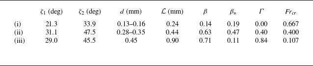


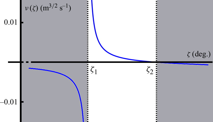


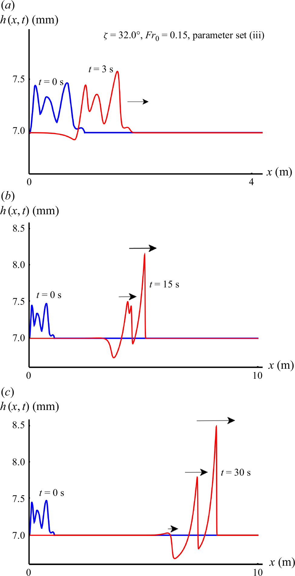


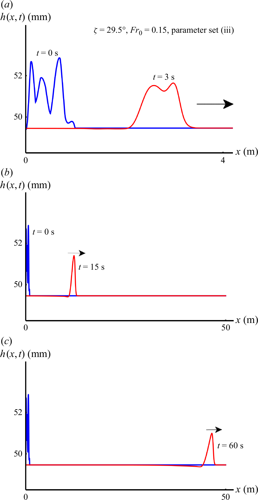


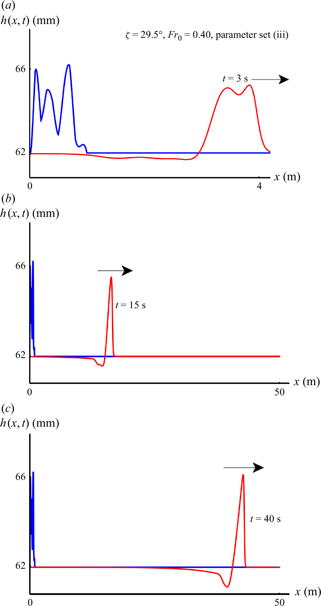


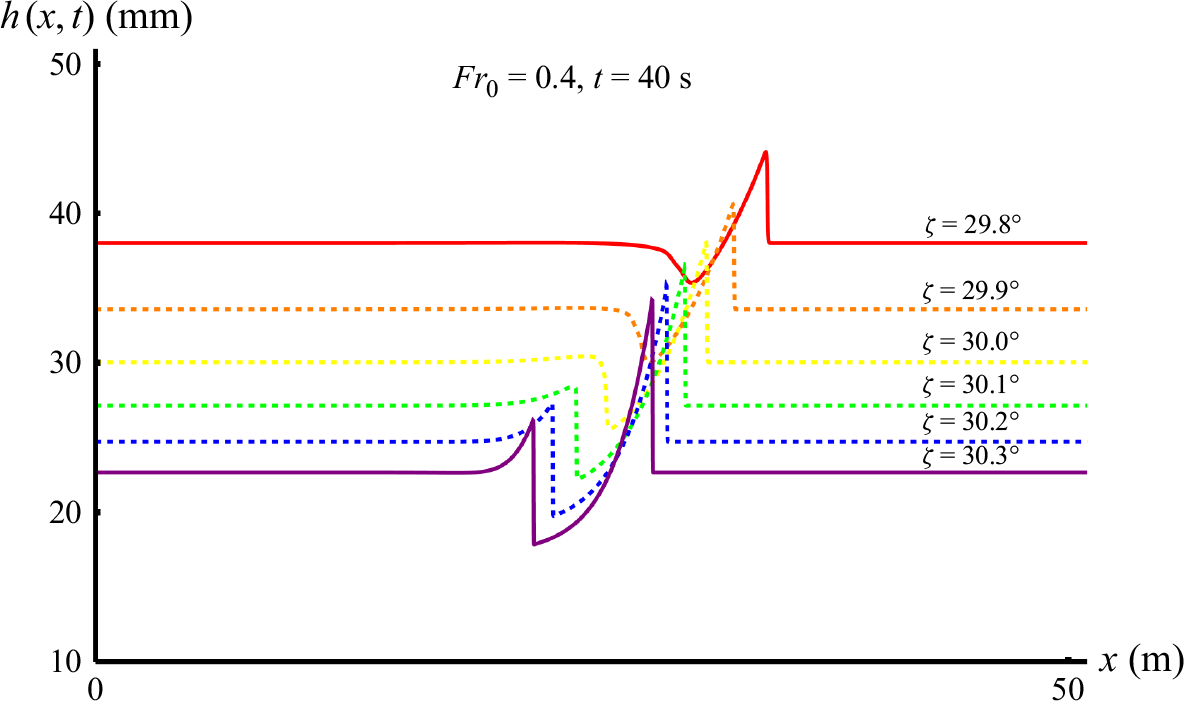


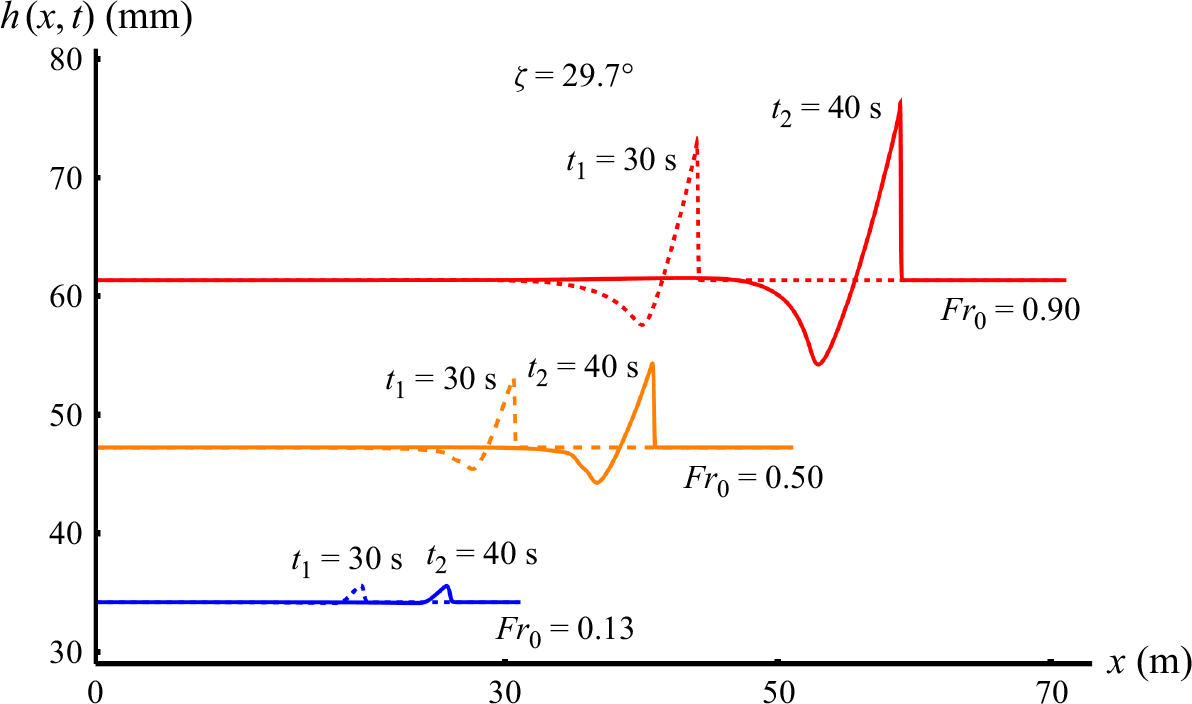


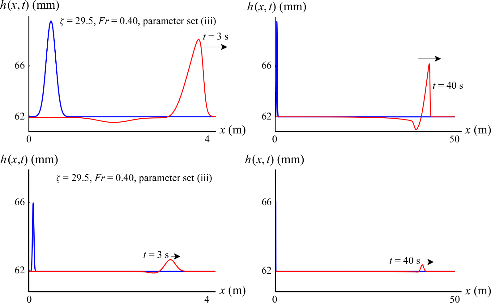


 Open access