


1. Introduction
Gravity currents are characterised by the penetration of one fluid layer into another with a different density due to horizontal pressure gradients induced by density differences. Such density differences may arise, for example, as a result of temperature and salinity variations, dissolved substances or suspended particles. Owing to their relative thinness, horizontal motions within gravity currents dominate vertical motions, and often the domain of study of gravity currents is constrained by top and/or bottom boundaries. Examples of natural gravity currents include sea breezes, thunderstorm outflows, haboobs (a type of dust storm), turbidity currents, salinity intrusions, air intrusions associated with downdrafts accompanying atmospheric convection during thunderstorms known as cold pools (Phadtare et al. Reference Phadtare2024) and powder-snow avalanches (Hopfinger Reference Hopfinger1983; Huppert Reference Huppert2006). Atmospheric gravity currents on (gently) sloping radiatively cooled surfaces (i.e. katabatic flows) have also been a topic of continuing interest (Farina & Zardi Reference Farina and Zardi2023).
The interaction of gravity currents with obstacles has been investigated in the context of numerous engineering applications, including the containment of accidentally released toxic dense gases (Rottman et al. Reference Rottman, Simpson and Hunt1985; Lane-Serff et al. Reference Lane-Serff, Beal and Hadfield1995; Skevington & Hogg Reference Skevington and Hogg2023), submarine cable ruptures (Heezen & Ewing Reference Heezen and Ewing1952; Krause et al. Reference Krause, White, Piper and Heezen1970; Cattaneo et al. Reference Cattaneo, Babonneau, Ratzov, Dan-Unterseh, Yelles, Bracène, Lépinay, Boudiaf and Déverchère2012), sediment diversions (Oehy et al. Reference Oehy, De Cesare and Schleiss2010), pollutant plumes at oceanic and atmospheric outfalls (Chowdhury & Testik Reference Chowdhury and Testik2014), and dynamic loading on submarine structures (Gonzalez-Juez & Meiburg Reference Gonzalez-Juez and Meiburg2009; Wu & Ouyang Reference Wu and Ouyang2020). Pioneering theoretical studies on gravity-current/obstacle interactions have been conducted using shallow water models by Rottman et al. (Reference Rottman, Simpson and Hunt1985), which were followed by those of Lane-Serff et al. (Reference Lane-Serff, Beal and Hadfield1995). Various numerical and theoretical models have been developed in two (2-D) and three dimensions to study such interactions, in particular for turbidity currents (Gonzalez-Juez et al. Reference Gonzalez-Juez, Meiburg and Constantinescu2009; Gonzalez-Juez & Meiburg Reference Gonzalez-Juez and Meiburg2009; Tokyay et al. Reference Tokyay, Constantinescu and Meiburg2012; Nasr-Azadani & Meiburg Reference Nasr-Azadani and Meiburg2014; Ozan et al. Reference Ozan, Constantinescu and Hogg2015; Tokyay & Constantinescu Reference Tokyay and Constantinescu2015; Jung & Yoon Reference Jung and Yoon2016; Nasr-Azadani et al. Reference Nasr-Azadani, Meiburg and Kneller2018; Wu & Ouyang Reference Wu and Ouyang2020) and unsteady gravity currents (Greenspan & Young Reference Greenspan and Young1978; Skevington & Hogg Reference Skevington and Hogg2023). Also, laboratory studies have been reported on the interaction of gravity currents (Bardoel et al. Reference Bardoel, Muñoz, Grachev, Krishnamurthy, Chamorro and Fernando2021) and turbidity currents (Wilson et al. Reference Wilson, Friedrich and Stevens2018, Reference Wilson, Friedrich and Stevens2019) with steep obstacles as well as on collisions between symmetric gravity currents (Zhong et al. Reference Zhong, Hussain and Fernando2018). Collisions of symmetric (Dai et al. Reference Dai, Huang and Wu2023) and asymmetric (Kokkinos & Prinos Reference Kokkinos and Prinos2023) gravity currents have also been studied numerically.
When a gravity current meets an isolated bottom-mounted obstacle, some of the fluid flows over (or around) the obstacle, while the remainder is reflected upstream as a propagating hydraulic jump or a bore. Often, this problem is studied in a 2-D configuration where the gravity current meets an obstacle located parallel to the front. Rottman et al. (Reference Rottman, Simpson and Hunt1985), Lane-Serff et al. (Reference Lane-Serff, Beal and Hadfield1995) and Skevington & Hogg (Reference Skevington and Hogg2023) quantified the fraction of the mass flux that continues over the obstacle as a function of the normalised obstacle height using shallow-water theory, which generally agreed with laboratory observations. Gonzalez-Juez & Meiburg (Reference Gonzalez-Juez and Meiburg2009) used high resolution Navier–Stokes simulations to study unsteady drag and lift forces associated with impinging gravity currents on bottom-mounted obstacles, and found that the impact stage is dominated by 2-D motions. Shallow-water models assume no mixing between the gravity current and the ambient fluid, an assumption unsuitable especially for blunt obstacles, wherein the gravity current deflects upward during the collision, separates from the bottom wall and thereafter flows over the top of the obstacle. Bardoel et al. (Reference Bardoel, Muñoz, Grachev, Krishnamurthy, Chamorro and Fernando2021) demonstrated significant mixing in such cases, thus demonstrating the limited applicability of hydraulic theory. The large eddy simulation (LES) by Wu & Ouyang (Reference Wu and Ouyang2020) indicates that mixing is intense for thin obstacles (a width-to-height ratio $w_0/h_0 \lt 0.2$
), whereas for wider obstacles, the gravity current reattaches to the obstacle, yielding lesser mixing.
$w_0/h_0 \lt 0.2$
), whereas for wider obstacles, the gravity current reattaches to the obstacle, yielding lesser mixing.
This study addresses knowledge gaps pertinent to flow evolution and turbulent mixing occurring during the interaction between a gravity current and an obstacle. The motivation was provided by field observations made during the ‘Toward Improving Coastal Fog Prediction’ (C-FOG) project (Fernando et al. Reference Fernando2021), where a cold front travelling over the northern Atlantic Ocean collided with a long promontory of Newfoundland (Bardoel et al. Reference Bardoel, Muñoz, Grachev, Krishnamurthy, Chamorro and Fernando2021), locally producing fog that lasted for tens of minutes. The collision increased the turbulent kinetic energy (TKE), its dissipation rate, as well as the root-mean-square temperature fluctuations measured on the promontory. It was hypothesised that this enhanced turbulence caused warm near-saturated ambient air over the promontory to mix with colder near-saturated air of the cold front, resulting in ‘mixing fog’ as postulated by Taylor (Reference Taylor1917). Accordingly, two near-saturated air masses of different temperature turbulently mix to form a saturated (foggy) airmass.
While observational platforms such as Doppler lidars, radars and instrumented aircrafts have recently provided important new information on gravity currents, their interactions with obstacles and phenomena ensued such as fog (Fernando et al. Reference Fernando2021; Phadtare et al. Reference Phadtare2024), field instrumentation has severe limitations in capturing and parametrising turbulent mixing processes. Traditionally, laboratory experiments and numerical simulations have been used to fill this niche. For example, the laboratory experiments of Bardoel et al. (Reference Bardoel, Muñoz, Grachev, Krishnamurthy, Chamorro and Fernando2021) identified space–time scales of turbulence generated during the collision, and suggested that mixing therein belongs to the subgrid category ( ${\sim}100$
–300 m) of the current operational atmospheric mesoscale numerical weather prediction (NWP) models, the highest horizontal resolution of which is
${\sim}100$
–300 m) of the current operational atmospheric mesoscale numerical weather prediction (NWP) models, the highest horizontal resolution of which is ${\sim}1$
km. Therefore, the prediction of fog due to gravity-current/obstacle collisions crucially depends on the fidelity of sub-grid eddy-diffusivity parametrisations used in NWP models. Even the currently available high-resolution (50 m horizontal grid) NWP models, for example, LES versions of the Weather Research and Forecasting model (WRF–LES) failed to predict the extent of local mixing during gravity-current/obstacle interactions (Dimitrova et al. Reference Dimitrova, Fernando, Silver, Bardoel, Dorman, Koračin, Vladimirov and Giani2025). The present work employs laboratory experiments to address this problem and to develop a suitable eddy-diffusivity parametrisation implementable in NWP models.
${\sim}1$
km. Therefore, the prediction of fog due to gravity-current/obstacle collisions crucially depends on the fidelity of sub-grid eddy-diffusivity parametrisations used in NWP models. Even the currently available high-resolution (50 m horizontal grid) NWP models, for example, LES versions of the Weather Research and Forecasting model (WRF–LES) failed to predict the extent of local mixing during gravity-current/obstacle interactions (Dimitrova et al. Reference Dimitrova, Fernando, Silver, Bardoel, Dorman, Koračin, Vladimirov and Giani2025). The present work employs laboratory experiments to address this problem and to develop a suitable eddy-diffusivity parametrisation implementable in NWP models.
This paper is structured as follows. Section 2 outlines the problem being addressed, its scope, the design of laboratory experiments and the dimensionless parameters relevant to the study. Section 3 describes the experimental set-up and procedure. Section 4 provides a phenomenological overview of flow in obstructed gravity currents, dividing it into four distinct stages characterised by variations in front speed and density fields. Section 5 identifies the characteristic time scales pertinent to flow stages, which are critical for identifying different mixing regimes and the extrapolation of results to field cases. The evolution of TKE and turbulent mixing in various stages and an averaged eddy-diffusivity parametrisation are given in § § 6 and 7, respectively. A brief discussion of the results is given in § 8, and the paper concludes in § 9 with salient results of the paper and future research directions.
2. Problem statement and flow configuration
The aim of the present work is to identify dynamically disparate stages of flow evolution during the impingement of a gravity current on an isolated obstacle and to quantify turbulent mixing therein in terms of an eddy diffusivity.
Our approach is to study 2-D gravity currents in a laboratory setting, where, traditionally, gravity currents have been generated by lifting a gate (lock) separating a dense fluid layer of density $\rho _1$
confined to a small compartment of width
$\rho _1$
confined to a small compartment of width $L$
and height
$L$
and height $h_L$
, from a long lighter (ambient) layer of density
$h_L$
, from a long lighter (ambient) layer of density $\rho _{{a}}$
and depth
$\rho _{{a}}$
and depth $H$
, the density difference being small (i.e. the Boussinesq approximation is valid). This is the standard lock-exchange configuration, vis-à-vis the dam-break flows with larger density differences (Simpson Reference Simpson1982; Ungarish Reference Ungarish2020). Upon removing the lock, the denser fluid collapses, flows as a basal gravity current, and interacts with a slender obstacle of height
$H$
, the density difference being small (i.e. the Boussinesq approximation is valid). This is the standard lock-exchange configuration, vis-à-vis the dam-break flows with larger density differences (Simpson Reference Simpson1982; Ungarish Reference Ungarish2020). Upon removing the lock, the denser fluid collapses, flows as a basal gravity current, and interacts with a slender obstacle of height $h_0$
and width
$h_0$
and width $w_0$
that was placed at a distance
$w_0$
that was placed at a distance $x_0$
from the lock (figure 1). The external governing parameters before the onset of obstacle effects are (Zhong et al. Reference Zhong, Hussain and Fernando2018):
$x_0$
from the lock (figure 1). The external governing parameters before the onset of obstacle effects are (Zhong et al. Reference Zhong, Hussain and Fernando2018): $\rho _1$
,
$\rho _1$
, $\rho _{{a}}$
,
$\rho _{{a}}$
, $g$
(gravitational acceleration),
$g$
(gravitational acceleration), $H$
,
$H$
, $\overline {u}_{{f}}$
,
$\overline {u}_{{f}}$
, $h_{{g}}$
and
$h_{{g}}$
and $\nu$
(kinematic viscosity). To the Boussinesq approximation,
$\nu$
(kinematic viscosity). To the Boussinesq approximation, $\rho _1$
,
$\rho _1$
, $\rho _{{a}}$
and
$\rho _{{a}}$
and $g$
can be combined into the reduced gravity
$g$
can be combined into the reduced gravity $g' = g(\rho _1 - \rho _{{a}})/\rho _0$
, where
$g' = g(\rho _1 - \rho _{{a}})/\rho _0$
, where $\rho _0 = (\rho _1 + \rho _{{a}})/2$
is a reference density, thus yielding
$\rho _0 = (\rho _1 + \rho _{{a}})/2$
is a reference density, thus yielding $g'$
,
$g'$
, $H$
,
$H$
, $\overline {u}_{{f}}$
,
$\overline {u}_{{f}}$
, $h_{{g}}$
and
$h_{{g}}$
and $\nu$
as the set of external parameters.
$\nu$
as the set of external parameters.
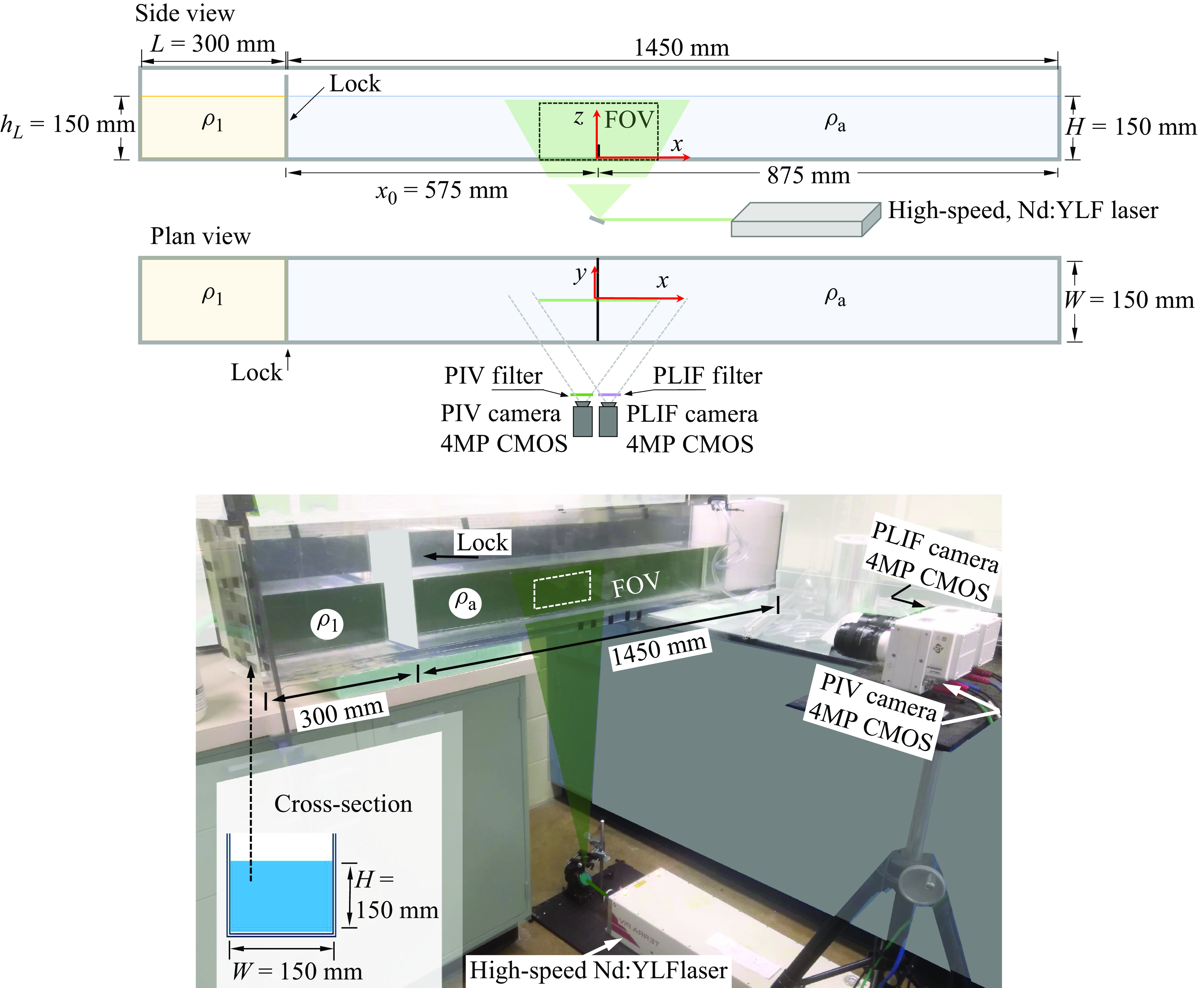
Schematics of the experimental arrangement employed to generate lock-exchange gravity currents. The gravity current was initiated by lifting the lock, and the diagram demonstrates the use of PIV (particle image velocimetry) and PLIF (planar laser-induced fluorescence) techniques. Note that the tank has a second lock compartment on the right-hand side of the tank for studies of colliding counterflowing gravity currents (Zhong et al. Reference Zhong, Hussain and Fernando2018), which was not used in the present experiments.
In the past, two lock-exchange configurations have typically been used for research: $h_L = H$
(full-depth case) and
$h_L = H$
(full-depth case) and $h_L \ll H$
(partial-depth case), the former being the most common (Simpson Reference Simpson1982; Shin et al. Reference Shin, Dalziel and Linden2004; Constantinescu Reference Constantinescu2014). For the atmospheric case of interest here, the cold front and mixing fog as observed during C-FOG appeared to have originated from a cold pool below the base of deep-convective cloud that conforms to
$h_L \ll H$
(partial-depth case), the former being the most common (Simpson Reference Simpson1982; Shin et al. Reference Shin, Dalziel and Linden2004; Constantinescu Reference Constantinescu2014). For the atmospheric case of interest here, the cold front and mixing fog as observed during C-FOG appeared to have originated from a cold pool below the base of deep-convective cloud that conforms to $h_L \approx H$
(e.g. Bardoel et al. Reference Bardoel, Muñoz, Grachev, Krishnamurthy, Chamorro and Fernando2021; Fernando et al. Reference Fernando2021; Phadtare et al. Reference Phadtare2024). Thus, the
$h_L \approx H$
(e.g. Bardoel et al. Reference Bardoel, Muñoz, Grachev, Krishnamurthy, Chamorro and Fernando2021; Fernando et al. Reference Fernando2021; Phadtare et al. Reference Phadtare2024). Thus, the $h_L = H$
(full depth) case was selected for the laboratory study. A notable feature of the full-depth case is the presence of a regime of uniform mean frontal velocity
$h_L = H$
(full depth) case was selected for the laboratory study. A notable feature of the full-depth case is the presence of a regime of uniform mean frontal velocity $\overline {u}_{{f}}$
that persists until the reflected lock-related disturbances from the end (back) wall catch up (Rottman & Simpson Reference Rottman and Simpson1983) and overtake the front after the front travels for
$\overline {u}_{{f}}$
that persists until the reflected lock-related disturbances from the end (back) wall catch up (Rottman & Simpson Reference Rottman and Simpson1983) and overtake the front after the front travels for ${\sim}10L$
(Simpson Reference Simpson1982) or more stringently,
${\sim}10L$
(Simpson Reference Simpson1982) or more stringently, ${\sim}5L$
(Skevington & Hogg Reference Skevington and Hogg2023). We opted to place the obstacle in this constant
${\sim}5L$
(Skevington & Hogg Reference Skevington and Hogg2023). We opted to place the obstacle in this constant $\overline {u}_{{f}}$
regime, where the influence of
$\overline {u}_{{f}}$
regime, where the influence of $L$
and the distance between the front and the lock could be neglected in interpreting results. Specifically, the barrier (obstacle) was placed at a distance
$L$
and the distance between the front and the lock could be neglected in interpreting results. Specifically, the barrier (obstacle) was placed at a distance $x_0 \approx 1.9L$
from the lock.
$x_0 \approx 1.9L$
from the lock.
Based on the above provisos, any parameter $\wp$
in the constant
$\wp$
in the constant $\overline {u}_{{f}}$
regime can be expressed as
$\overline {u}_{{f}}$
regime can be expressed as $\wp = \wp (g', H, \nu )$
. Thus, the functional (
$\wp = \wp (g', H, \nu )$
. Thus, the functional ( $\mathcal{F}$
) form of the front velocity becomes
$\mathcal{F}$
) form of the front velocity becomes $\overline {u}_{{f}}/\sqrt {g'H} = \mathcal{F}(\sqrt {g'H^3}/\nu )$
, where at sufficiently large Reynolds numbers, the dependence on
$\overline {u}_{{f}}/\sqrt {g'H} = \mathcal{F}(\sqrt {g'H^3}/\nu )$
, where at sufficiently large Reynolds numbers, the dependence on $\sqrt {g'H^3}/\nu$
is negligible, leading to a constant Froude number
$\sqrt {g'H^3}/\nu$
is negligible, leading to a constant Froude number $Fr = \overline {u}_{{f}}/\sqrt {g'H}$
. Similarly, the normalised gravity current height
$Fr = \overline {u}_{{f}}/\sqrt {g'H}$
. Similarly, the normalised gravity current height ${h_{{g}}}/H$
becomes constant in this regime. The idealised hydraulic theory of Benjamin (Reference Benjamin1968) indeed predicts
${h_{{g}}}/H$
becomes constant in this regime. The idealised hydraulic theory of Benjamin (Reference Benjamin1968) indeed predicts $Fr = 0.5$
and
$Fr = 0.5$
and ${h_{{g}}}/H = 0.5$
for full-depth lock releases, which are in general agreement with a range of laboratory observations (see Shin et al. Reference Shin, Dalziel and Linden2004). The introduction of an obstacle gives rise to the additional parameters
${h_{{g}}}/H = 0.5$
for full-depth lock releases, which are in general agreement with a range of laboratory observations (see Shin et al. Reference Shin, Dalziel and Linden2004). The introduction of an obstacle gives rise to the additional parameters $h_0$
and
$h_0$
and $w_0$
, but the aspect ratio used was
$w_0$
, but the aspect ratio used was $w_0/h_0\lt 0.05$
, thus ensuring that flow physics studied here is applicable for thin barriers with flow separation, according to the classification of Wu & Ouyang (Reference Wu and Ouyang2020). This leaves
$w_0/h_0\lt 0.05$
, thus ensuring that flow physics studied here is applicable for thin barriers with flow separation, according to the classification of Wu & Ouyang (Reference Wu and Ouyang2020). This leaves $h_0/H = h_0/2{h_{{g}}}$
as the only relevant non-dimensional parameter.
$h_0/H = h_0/2{h_{{g}}}$
as the only relevant non-dimensional parameter.
Additional benefits of using $h_L = H$
are the voluminous literature available on this case (e.g. Simpson Reference Simpson1982; Constantinescu Reference Constantinescu2014; Ungarish Reference Ungarish2020; Agrawal et al. Reference Agrawal, Ramesh, Zimmerman, Philip and Klewicki2021) and the reduction of the number of experiments (and hence the exorbitant cost due to refractive-index matching) due to the absence of the additional parameter
$h_L = H$
are the voluminous literature available on this case (e.g. Simpson Reference Simpson1982; Constantinescu Reference Constantinescu2014; Ungarish Reference Ungarish2020; Agrawal et al. Reference Agrawal, Ramesh, Zimmerman, Philip and Klewicki2021) and the reduction of the number of experiments (and hence the exorbitant cost due to refractive-index matching) due to the absence of the additional parameter $h_L$
. Furthermore, working in the
$h_L$
. Furthermore, working in the $h_L = H$
regime allows removal of
$h_L = H$
regime allows removal of $L$
(or
$L$
(or $L/H$
) in the analysis. It is emphasised, however, that the frontal flow structure in this regime may be different from those that develop when the barrier is far from the release, or when the barrier is placed much closer to the lock, both analysed by Skevington & Hogg (Reference Skevington and Hogg2023). Studies of such regimes are out of our scope since the interest here is to extend results to atmospheric gravity currents devoid of the influence of upstream ‘source’ conditions (that are ill-defined in nature). Therefore, the problem studied concerns flow regimes and turbulent mixing ensuing the impingement of a steady gravity current with an unperturbed (upstream) frontal velocity
$L/H$
) in the analysis. It is emphasised, however, that the frontal flow structure in this regime may be different from those that develop when the barrier is far from the release, or when the barrier is placed much closer to the lock, both analysed by Skevington & Hogg (Reference Skevington and Hogg2023). Studies of such regimes are out of our scope since the interest here is to extend results to atmospheric gravity currents devoid of the influence of upstream ‘source’ conditions (that are ill-defined in nature). Therefore, the problem studied concerns flow regimes and turbulent mixing ensuing the impingement of a steady gravity current with an unperturbed (upstream) frontal velocity $\overline {u}_{{f}}$
and depth
$\overline {u}_{{f}}$
and depth $h_{{g}}$
with a thin obstacle of height
$h_{{g}}$
with a thin obstacle of height $h_0$
at high Reynolds numbers
$h_0$
at high Reynolds numbers $Re = \overline {u}_{{f}}{h_{{g}}}/\nu$
.
$Re = \overline {u}_{{f}}{h_{{g}}}/\nu$
.
Here, turbulent mixing can be quantified by observing the evolution of the density $\rho$
or buoyancy
$\rho$
or buoyancy $b = -g(\rho - \rho _0)/\rho _0$
of fluid parcels that satisfies the following conservation equation:
$b = -g(\rho - \rho _0)/\rho _0$
of fluid parcels that satisfies the following conservation equation:
 \begin{equation} \frac {\partial \overline {b}}{\partial t} + \overline {u}_j \frac {\partial \overline {b}}{\partial x_j} = k \frac {\partial ^2 \overline {b}}{\partial x_j \partial x_j} - \frac {\partial \overline {b' u'_j}}{\partial x_j}, \end{equation}
where the overbar and prime denote the ensemble average and deviation from it, $u_j$
the velocity, and
$u_j$
the velocity, and $k$
the molecular diffusivity. The buoyancy flux
$k$
the molecular diffusivity. The buoyancy flux $\overline {b' u'_j}$
is parametrised using a domain-representative (spatially constant) eddy diffusivity
$\overline {b' u'_j}$
is parametrised using a domain-representative (spatially constant) eddy diffusivity $k_b$
,
$k_b$
,
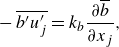 \begin{equation} -\overline {b'u'_j} = k_b \frac {\partial \overline {b}}{\partial x_j}, \end{equation}
leading to
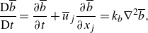 \begin{equation} \frac {\mathrm{D}\overline {b}}{\mathrm{D}t} = \frac {\partial \overline {b}}{\partial t} + \overline {u}_j \frac {\partial \overline {b}}{\partial x_j} = k_b \nabla ^2 \overline {b}, \end{equation}
since $k \ll k_b$
. Note that
$k \ll k_b$
. Note that $\mathrm{D}\overline {b}/\mathrm{D}t$
is used to represent the variation of mean buoyancy of a fluid parcel advected by the mean flow
$\mathrm{D}\overline {b}/\mathrm{D}t$
is used to represent the variation of mean buoyancy of a fluid parcel advected by the mean flow $\overline {u}_j$
, and not to represent the material derivative in the strict sense. For the problem in hand,
$\overline {u}_j$
, and not to represent the material derivative in the strict sense. For the problem in hand, $k_b$
varies in space and time, but the aim here is to find a spatially averaged
$k_b$
varies in space and time, but the aim here is to find a spatially averaged $k_b$
in a representative domain that encompasses the obstacle-induced mixing event. Such ‘conditional’ diffusivities are useful for implementation in NWP models and are activated in the model when criteria for the existence of a particular sub-grid phenomenon is satisfied. For example, a model could enable an eddy-diffusivity parametrisation of the form
$k_b$
in a representative domain that encompasses the obstacle-induced mixing event. Such ‘conditional’ diffusivities are useful for implementation in NWP models and are activated in the model when criteria for the existence of a particular sub-grid phenomenon is satisfied. For example, a model could enable an eddy-diffusivity parametrisation of the form $k_b = k_b(\overline {u}_{{f}}\!, H, h_0)$
or
$k_b = k_b(\overline {u}_{{f}}\!, H, h_0)$
or $k_b/\overline {u}_{{f}} H = f(h_0/H) = f(h_0/2{h_{{g}}})$
over the duration of an (enhanced) mixing event induced by a gravity-current/obstacle collision in a model grid cell, where
$k_b/\overline {u}_{{f}} H = f(h_0/H) = f(h_0/2{h_{{g}}})$
over the duration of an (enhanced) mixing event induced by a gravity-current/obstacle collision in a model grid cell, where $f$
is a function to be determined using laboratory studies. As such, it is important to know both the function
$f$
is a function to be determined using laboratory studies. As such, it is important to know both the function $f$
, and the extent and duration of a collision event, which is sought in this paper.
$f$
, and the extent and duration of a collision event, which is sought in this paper.
3. Experimental set-up
3.1. Lock-exchange apparatus
The experiments were carried out in a 1750 mm long, 150 mm wide and 300 mm high Plexiglas tank. A gate was positioned 300 mm from the left side of the tank to separate the dense fluid (density $\rho _1$
) from the lighter fluid (
$\rho _1$
) from the lighter fluid ( $\rho _{{a}}$
). A high-speed, dual cavity Amplitude Terra Nd:YLF laser (527 nm) generated a 2 mm thick laser sheet that illuminated the vertical plane in the centre of the tank (
$\rho _{{a}}$
). A high-speed, dual cavity Amplitude Terra Nd:YLF laser (527 nm) generated a 2 mm thick laser sheet that illuminated the vertical plane in the centre of the tank ( $y = 0$
). The velocity and density fields were captured simultaneously with a time-resolved PIV/PLIF system using two cameras. A schematic of the experimental set-up is shown in figure 1.
$y = 0$
). The velocity and density fields were captured simultaneously with a time-resolved PIV/PLIF system using two cameras. A schematic of the experimental set-up is shown in figure 1.
A variety of gravity currents interacting with isolated obstacles spanning the full width of the tank was investigated. This included three obstacle heights ( $h_0$
) and two Reynolds numbers (
$h_0$
) and two Reynolds numbers ( $Re$
) for each obstacle scenario, as well as two base cases with
$Re$
) for each obstacle scenario, as well as two base cases with $h_0 = 0$
for each
$h_0 = 0$
for each $Re$
. The coordinate system was centred at the base of the obstacle, coinciding with the middle of the measurement window. The streamwise, spanwise and vertical coordinates are denoted by
$Re$
. The coordinate system was centred at the base of the obstacle, coinciding with the middle of the measurement window. The streamwise, spanwise and vertical coordinates are denoted by $x$
,
$x$
, $y$
and
$y$
and $z$
, respectively. The obstacles were made using a thin aluminium sheet of width
$z$
, respectively. The obstacles were made using a thin aluminium sheet of width $w_0 \approx 0.5\,\rm mm$
, mounted securely to the bottom of the tank. The laser was placed right below the obstacle to minimise the shadow immediately above the obstacle. The dense and lighter fluids were formed using salt and an aqueous ethanol solution, respectively. Fluid densities were selected to ensure a uniform refractive index throughout the tank to minimise light and optical distortions. The technique for refractive-index matching used here is detailed by Hannoun et al. (Reference Hannoun, Fernando and List1988), Strang & Fernando (Reference Strang and Fernando2001) and Xu & Chen (Reference Xu and Chen2012). The experimental parameters are summarised in table 1.
$w_0 \approx 0.5\,\rm mm$
, mounted securely to the bottom of the tank. The laser was placed right below the obstacle to minimise the shadow immediately above the obstacle. The dense and lighter fluids were formed using salt and an aqueous ethanol solution, respectively. Fluid densities were selected to ensure a uniform refractive index throughout the tank to minimise light and optical distortions. The technique for refractive-index matching used here is detailed by Hannoun et al. (Reference Hannoun, Fernando and List1988), Strang & Fernando (Reference Strang and Fernando2001) and Xu & Chen (Reference Xu and Chen2012). The experimental parameters are summarised in table 1.
Basic experimental parameters. All cases shared the depth of the ambient fluid layer, $H = 15\,\rm cm$
. The velocity scale was determined using
$H = 15\,\rm cm$
. The velocity scale was determined using $\overline {u}_{{f}} = Fr \sqrt {g'H}$
with
$\overline {u}_{{f}} = Fr \sqrt {g'H}$
with $Fr = 0.45$
, derived from the two unobstructed cases. All the cases share a resolution of 7.3 pixel mm
$Fr = 0.45$
, derived from the two unobstructed cases. All the cases share a resolution of 7.3 pixel mm $^{-1}$
.
$^{-1}$
.

3.2. Velocity measurements
High-speed PIV was used to characterise the velocity fields in the $x$
–
$x$
– $z$
plane. Both fluids were seeded with silver-coated hollow ceramic spheres with a diameter of 50
$z$
plane. Both fluids were seeded with silver-coated hollow ceramic spheres with a diameter of 50 $\unicode {x03BC}$
m that were illuminated using an 80 W Terra laser. A Phantom M340 high-speed camera, equipped with a 2560
$\unicode {x03BC}$
m that were illuminated using an 80 W Terra laser. A Phantom M340 high-speed camera, equipped with a 2560 $\times$
1600 pixels CMOS sensor, captured sets of 2000 PIV images for each of the eighty runs (four obstacle configurations, two
$\times$
1600 pixels CMOS sensor, captured sets of 2000 PIV images for each of the eighty runs (four obstacle configurations, two $Re$
and 10 runs per case). A low-pass filter with a cut-off wavelength of 550 nm filtered out the fluorescence originating from the fluorescent dye used for the PLIF measurements. The PIV images were processed using the TSI Insight 4G software with final interrogation windows of 32
$Re$
and 10 runs per case). A low-pass filter with a cut-off wavelength of 550 nm filtered out the fluorescence originating from the fluorescent dye used for the PLIF measurements. The PIV images were processed using the TSI Insight 4G software with final interrogation windows of 32 $\times$
32 pixels and a 50 % overlap; this resulted in a grid spacing between individual velocity vectors of
$\times$
32 pixels and a 50 % overlap; this resulted in a grid spacing between individual velocity vectors of $\Delta x = \Delta z = 2.2\,\rm mm$
.
$\Delta x = \Delta z = 2.2\,\rm mm$
.
3.3. Density measurements
Time-resolved PLIF was employed to measure the density field. Rhodamine 6G (R6G) was used as the fluorescent dye due to its resistance to photo-bleaching, high quantum efficiency and its absorption peak (525 nm) being close to the laser wavelength (527 nm) (Crimaldi Reference Crimaldi2008). Great care was taken in handling and disposing R6G per material safety data sheets, which increased the cost of each experiment substantially. The dye was added solely to the lighter fluid at a starting concentration of 65 $\unicode {x03BC}$
g L
$\unicode {x03BC}$
g L $^{-1}$
. A second Phantom M340 camera, equipped with a 2560
$^{-1}$
. A second Phantom M340 camera, equipped with a 2560 $\times$
1600 pixels CMOS sensor, recorded the fluorescence spectrum. A high-pass filter with a cutoff wavelength of 550 nm was used to filter out the laser light. The calibration technique outlined by Xu & Chen (Reference Xu and Chen2012) was used to compute R6G concentrations from greyscale values. Density fields were then computed from the R6G concentration by employing a linear calibration method.
$\times$
1600 pixels CMOS sensor, recorded the fluorescence spectrum. A high-pass filter with a cutoff wavelength of 550 nm was used to filter out the laser light. The calibration technique outlined by Xu & Chen (Reference Xu and Chen2012) was used to compute R6G concentrations from greyscale values. Density fields were then computed from the R6G concentration by employing a linear calibration method.
3.4. Phase-aligned ensemble averaging technique
Turbulence statistics of gravity currents were obtained using ensemble averaging considering the high spatial inhomogeneity and non-stationarity of gravity currents. To ensure statistical significance, ten independent runs were performed for each experimental configuration. This number was determined by logistical constraints that required 190-proof ethanol for refractive-index matching and the professional disposal of R6G contaminated fluid after each experiment. The non-simultaneity of gravity-current impingement on the obstacle due to minor differences in the initial conditions and flow development required the application of the phase-aligned ensemble averaging technique (PAET). This technique iteratively maximises the cross-correlation of the ensemble average with the ten individual realisations, and shifts the time and space dimensions accordingly. While alignment was necessary for the time dimension, the horizontal variations were limited by the obstacle and the vertical variations were limited by the bottom of the tank. Further information on the application of PAET for gravity current experiments can be found from Zhong et al. (Reference Zhong, Hussain and Fernando2018, Reference Zhong, Hussain and Fernando2020). Obviously, the small number of realisations used for a single ensemble average may lead to larger uncertainties, which is discussed in § 8.
4. Phenomenological overview
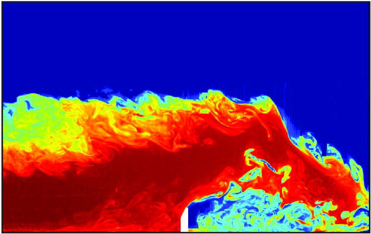
Instantaneous density fields $\rho$
for the (a1
$\rho$
for the (a1 $-$
d1) C5200H0.1 and (a2
$-$
d1) C5200H0.1 and (a2 $-$
d2) C5200H0.3 cases. Individual realisations are shown. The annotations show key flow features during the collision.
$-$
d2) C5200H0.3 cases. Individual realisations are shown. The annotations show key flow features during the collision.

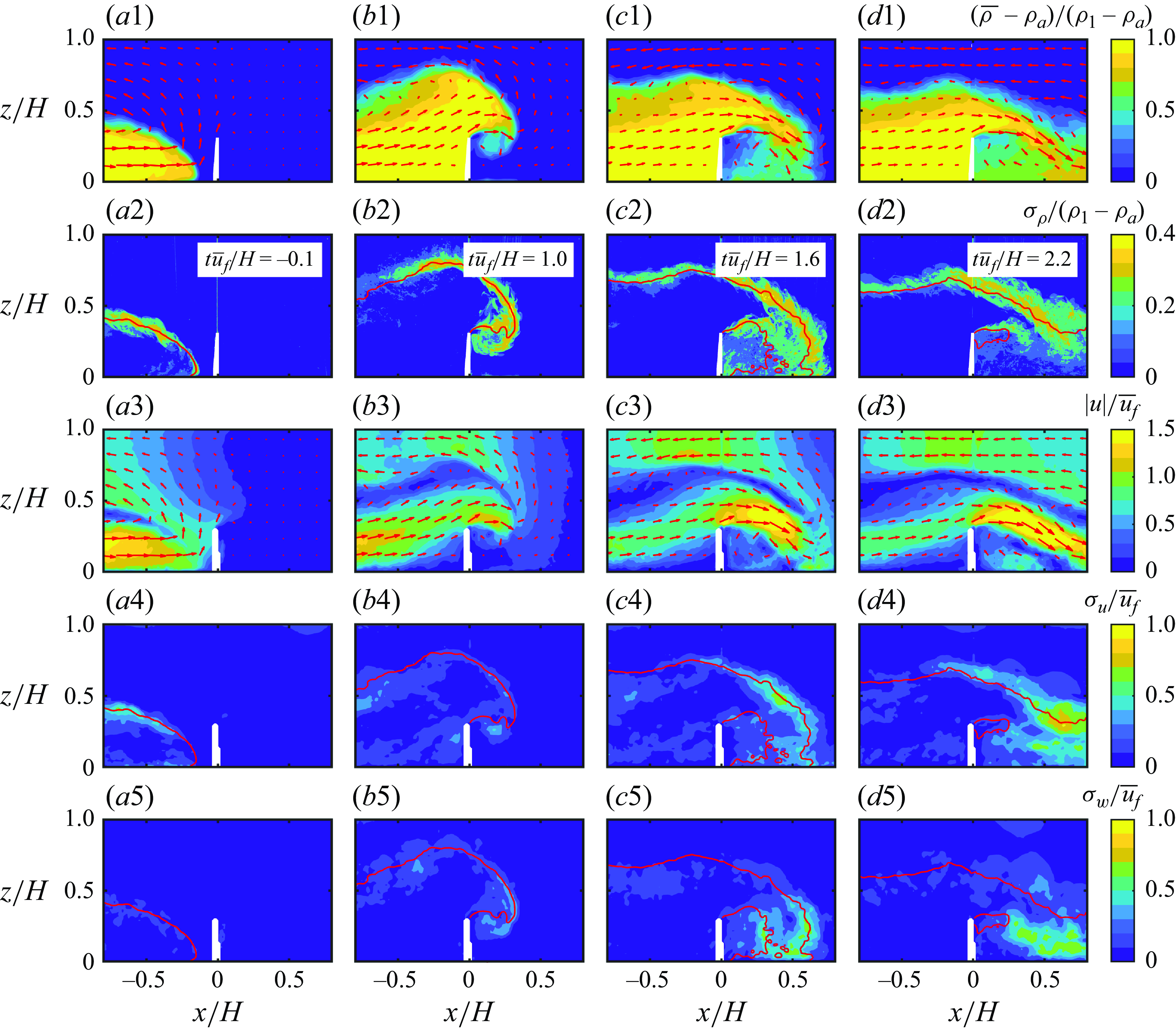
After the lock release, gravity currents propagated towards the obstacle and interacted with it. Figure 2 presents the evolution of instantaneous density field in two obstructed runs illustrating this interaction (C5200H0.1 and C5200H0.3; see table 1 and note the terminology – Reynolds number and normalised obstacle height). Figure 3 displays ensemble averaged density and velocity fields, along with their associated fluctuations, for one of the cases in figure 2 (C5200H0.3), captured at various moments in time. The other cases show similar behaviour, and are not shown for brevity. Note that the PIV and PLIF cameras were positioned slightly to the left and right of the obstacle, leading to a partial obstruction of the field of view for both cameras and causing the obstacle to appear as a parallelogram instead of a thin vertical line in figure 2.
Ensemble fields of density, density fluctuations $\sigma _{\rho }$
, flow speed, horizontal and vertical velocity fluctuations
$\sigma _{\rho }$
, flow speed, horizontal and vertical velocity fluctuations $\sigma _u$
and
$\sigma _u$
and $\sigma _w$
superimposed with either velocity vectors or the
$\sigma _w$
superimposed with either velocity vectors or the $\overline {\rho } = (\rho _1 + \rho _{{a}})/2$
contour for the C5200H0.3 case at (a)
$\overline {\rho } = (\rho _1 + \rho _{{a}})/2$
contour for the C5200H0.3 case at (a) $t \overline {u}_{{f}}/H = -0.1$
, (b) 1.0, (c) 1.6 and (d) 2.2.
$t \overline {u}_{{f}}/H = -0.1$
, (b) 1.0, (c) 1.6 and (d) 2.2.
The gravity current, as characterised using the frontal velocity, could be categorised upon careful examination into four distinct stages. The initial lock-exchange flow is the first stage, where the gravity current stabilises to produce a nearly constant front speed, during which Kelvin–Helmholtz (KH)-type billows emerge in the shear layer at the periphery of the gravity current, coupled with lobe and cleft instabilities at the nose of the gravity current (Simpson Reference Simpson1982). The current remains largely uninfluenced by the obstacle until contact is made with the obstacle at time $t = 0$
, although some upstream influence is expected because of the irrotational motions induced ahead (Bardoel et al. Reference Bardoel, Muñoz, Grachev, Krishnamurthy, Chamorro and Fernando2021).
$t = 0$
, although some upstream influence is expected because of the irrotational motions induced ahead (Bardoel et al. Reference Bardoel, Muñoz, Grachev, Krishnamurthy, Chamorro and Fernando2021).
The second stage begins once the gravity current touches the obstacle and deflects upward likely due to a rise of pressure in the front face of the obstacle, during which the gravity current resembles a ‘negatively buoyant jet’ that rises (see figure 2 b), decelerates and eventually reaches its maximum height. The features of a hydraulic jump appear as the gravity current spills over the topography, where a part of it is reflected upstream (figures 2 b2, 2 c2; 3 b1, 3 c1). This adjustment appears to establish the flow over the obstacle; an overtopping current, a reverse flow alof and a shear-layer in between (figures 2 c1, 2 c2; 3 b1, 3 c1), causing shear-induced mixing at the top of the overtopping current (figure 2 c1, c2). After the collision, a vortex forms underneath the gravity current that spills over the obstacle, typical of flow separation (see figure 2 b).
The third stage is characterised by the collapse of the gravity current flowing over the obstacle, which descends back to the bottom surface (figure 2
c). In this stage, the frontal area accelerates as it moves diagonally downward, reaching the bottom surface at approximately $x/H \approx 0.75$
. Therein, instabilities manifest above and below the gravity current, leading to enhanced mixing. The top surface of the current overtopping flow is a stably stratified shear flow with propensity for KH instabilities, and the physical appearance of the instabilities resembled KH billows, for example, previously reported by Thorpe (Reference Thorpe1973,Reference Thorpe1987). Detailed observations of KH-billow breakdown show that the maximum amplitude is achieved at the dimensionless time
$x/H \approx 0.75$
. Therein, instabilities manifest above and below the gravity current, leading to enhanced mixing. The top surface of the current overtopping flow is a stably stratified shear flow with propensity for KH instabilities, and the physical appearance of the instabilities resembled KH billows, for example, previously reported by Thorpe (Reference Thorpe1973,Reference Thorpe1987). Detailed observations of KH-billow breakdown show that the maximum amplitude is achieved at the dimensionless time $\Delta U t/\lambda \approx 5$
, where
$\Delta U t/\lambda \approx 5$
, where $\Delta U$
is the shear across the interface and
$\Delta U$
is the shear across the interface and $\lambda$
the separation between the billows (De Silva et al. Reference De Silva, Fernando, Eaton and Hebert1996). Observations of all runs show that this criterion is satisfied and hence KH instabilities are possibly present on the top interface (figure 2
c,d). The bottom surface is inherently unstable, possibly with sheared Rayleigh–Taylor (RT) instabilities and hence is characterised by stronger turbulent mixing (figure 2
c,d). To our knowledge, there is no simple criterion available for the identification of sheared RT instabilities.
$\lambda$
the separation between the billows (De Silva et al. Reference De Silva, Fernando, Eaton and Hebert1996). Observations of all runs show that this criterion is satisfied and hence KH instabilities are possibly present on the top interface (figure 2
c,d). The bottom surface is inherently unstable, possibly with sheared Rayleigh–Taylor (RT) instabilities and hence is characterised by stronger turbulent mixing (figure 2
c,d). To our knowledge, there is no simple criterion available for the identification of sheared RT instabilities.
The fourth stage begins when the gravity current makes contact with the bottom surface following its collapse. It adjusts and continues its horizontal propagation over the bottom surface (figure 2 d). This stage has some similarities to the first stage. A recirculation zone is formed downstream of the obstacle, into which dense fluid from the gravity current is entrained. This process, over time, leads to more homogeneous densities at the bottom of the gravity current in the recirculating cavity, as evidenced in figures 2 and 3(c1,d1). While the time evolution of the recirculation bubble is of interest, the experiment did not last long enough to study a possible steady state that would have occurred if the gravity current were continuous. Occasionally, a secondary hydraulic jump was observed downstream of the obstacle, although it typically occurred beyond the limits of the measurement window.
5. Propagation of gravity currents during the collision
As discussed in § § 1 and 2, the front speed is a key parameter in the dynamics of obstructed gravity currents. This section analyses the modification of the front speed for varying obstacle heights and identifies an appropriate time scale, $t_*$
, to accurately define the duration of the four stages described in § 4. The time scale
$t_*$
, to accurately define the duration of the four stages described in § 4. The time scale $t_*$
also serves as a critical scaling factor for the time coordinate in evaluating turbulence and mixing across different obstacle heights in § § 6 and 7. Also, this section includes a brief discussion on the blocking effect of the obstacle.
$t_*$
also serves as a critical scaling factor for the time coordinate in evaluating turbulence and mixing across different obstacle heights in § § 6 and 7. Also, this section includes a brief discussion on the blocking effect of the obstacle.
5.1. Horizontal motion
Figure 4(a,b) illustrates the front position $x_{{f}}(t)$
and speed
$x_{{f}}(t)$
and speed $u_{{f}}(t)$
as a function of dimensionless time. The normalisation has been done using
$u_{{f}}(t)$
as a function of dimensionless time. The normalisation has been done using $H$
, the averaged upstream (stage I) frontal velocity scale
$H$
, the averaged upstream (stage I) frontal velocity scale $\overline {u}_{{f}}$
, and time scale
$\overline {u}_{{f}}$
, and time scale $t_{*1} = H/\overline {u}_{{f}}$
. The inflection point of the
$t_{*1} = H/\overline {u}_{{f}}$
. The inflection point of the $\overline {\rho } = (\rho _1 + \rho _{{a}})/2$
contour was used to determine the front position as done by Gonzalez-Juez & Meiburg (Reference Gonzalez-Juez and Meiburg2009) and the time derivative of
$\overline {\rho } = (\rho _1 + \rho _{{a}})/2$
contour was used to determine the front position as done by Gonzalez-Juez & Meiburg (Reference Gonzalez-Juez and Meiburg2009) and the time derivative of $x_{{f}}$
gives the front speed.
$x_{{f}}$
gives the front speed.
As mentioned earlier, in the two (unobstructed) base cases (table 1), the gravity currents exhibit a constant front speed after their initial development, a stage commonly referred to as the slumping phase. It typically lasts for 5 $-$
10 lock lengths
$-$
10 lock lengths $L$
(Meiburg & Kneller Reference Meiburg and Kneller2010) and therefore, the barrier located at a distance
$L$
(Meiburg & Kneller Reference Meiburg and Kneller2010) and therefore, the barrier located at a distance $x_0 = 1.9L$
from the lock encounters gravity currents within this phase. Indeed, figure 4(a,b) demonstrates a constant velocity regime (in blue). Benjamin (Reference Benjamin1968) proposed
$x_0 = 1.9L$
from the lock encounters gravity currents within this phase. Indeed, figure 4(a,b) demonstrates a constant velocity regime (in blue). Benjamin (Reference Benjamin1968) proposed $Fr = 0.5$
for the slumping phase, but previous laboratory experiments and numerical simulations suggest a range of values for
$Fr = 0.5$
for the slumping phase, but previous laboratory experiments and numerical simulations suggest a range of values for $Fr$
between 0.38 and 0.48 (Huppert & Simpson Reference Huppert and Simpson1980; Härtel et al. Reference Härtel, Meiburg and Necker2000; Zhong et al. Reference Zhong, Hussain and Fernando2018; Pelmard et al. Reference Pelmard, Norris and Friedrich2020; Bardoel et al. Reference Bardoel, Muñoz, Grachev, Krishnamurthy, Chamorro and Fernando2021). In our study, for the two unobstructed cases,
$Fr$
between 0.38 and 0.48 (Huppert & Simpson Reference Huppert and Simpson1980; Härtel et al. Reference Härtel, Meiburg and Necker2000; Zhong et al. Reference Zhong, Hussain and Fernando2018; Pelmard et al. Reference Pelmard, Norris and Friedrich2020; Bardoel et al. Reference Bardoel, Muñoz, Grachev, Krishnamurthy, Chamorro and Fernando2021). In our study, for the two unobstructed cases, $Fr \approx 0.45 \pm 0.01$
, which was used to determine the scale
$Fr \approx 0.45 \pm 0.01$
, which was used to determine the scale $\overline {u}_{{f}} = Fr \sqrt {g'H}$
(table 1). Note that the slumping phase coincides with stage I.
$\overline {u}_{{f}} = Fr \sqrt {g'H}$
(table 1). Note that the slumping phase coincides with stage I.
Plots of the (a) front position $x_{{f}}$
and (b) front speed
$x_{{f}}$
and (b) front speed $u_{{f}}$
as a function of time, normalised by
$u_{{f}}$
as a function of time, normalised by $t_{*1} = H/\overline {u}_{{f}}$
. Panels (c) and (d) show the same variables against time with normalisation
$t_{*1} = H/\overline {u}_{{f}}$
. Panels (c) and (d) show the same variables against time with normalisation $t_{*3} = H/\overline {u}_{{f}} + 4.5h_0/\overline {u}_{{f}}$
. The solid and dashed lines are for the lower and higher
$t_{*3} = H/\overline {u}_{{f}} + 4.5h_0/\overline {u}_{{f}}$
. The solid and dashed lines are for the lower and higher $Re$
cases, respectively.
$Re$
cases, respectively.
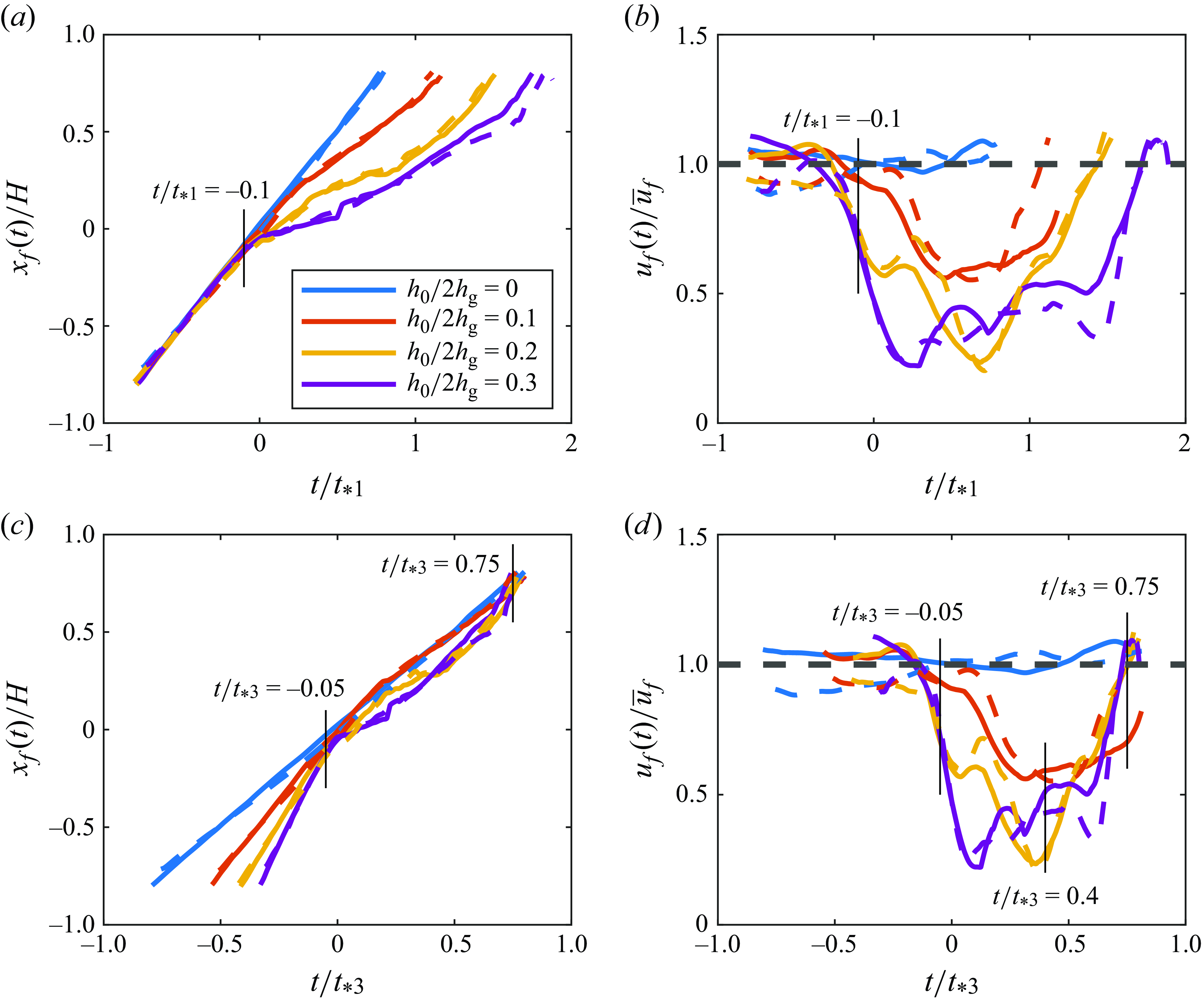
Before the impact with the obstacle at $x = 0$
and
$x = 0$
and $t = 0$
, the propagation characteristics of the obstructed gravity currents (e.g. front speed, height) are much the same as those of their unobstructed counterparts. The influence of the obstruction sets in only a short time before the collision, after which an abrupt reduction of the front speed could be seen, leading to a temporary decrease in speed. Subsequently, the obstructed gravity currents regain their initial front velocity after travelling a distance of
$t = 0$
, the propagation characteristics of the obstructed gravity currents (e.g. front speed, height) are much the same as those of their unobstructed counterparts. The influence of the obstruction sets in only a short time before the collision, after which an abrupt reduction of the front speed could be seen, leading to a temporary decrease in speed. Subsequently, the obstructed gravity currents regain their initial front velocity after travelling a distance of ${\sim}0.75H$
from the obstruction. It is striking that the gravity current nearly regains its initial speed following the collision, which is not expected given the perceived reduction in reduced gravity (
${\sim}0.75H$
from the obstruction. It is striking that the gravity current nearly regains its initial speed following the collision, which is not expected given the perceived reduction in reduced gravity ( $g'$
) due to the entrainment of ambient fluid during the collision. While mixing is observed during the collision, it predominantly affects the upper and lower boundaries of the gravity current, and the density (and
$g'$
) due to the entrainment of ambient fluid during the collision. While mixing is observed during the collision, it predominantly affects the upper and lower boundaries of the gravity current, and the density (and $g'$
) at the centre (core) remain largely unchanged, as shown in figure 2(c1, c2), which may explain the above observation. This phenomenon aligns with the findings of Wu & Ouyang (Reference Wu and Ouyang2020, their figure 4), who also reported the ratio
$g'$
) at the centre (core) remain largely unchanged, as shown in figure 2(c1, c2), which may explain the above observation. This phenomenon aligns with the findings of Wu & Ouyang (Reference Wu and Ouyang2020, their figure 4), who also reported the ratio $u_{{f}}/\overline {u}_{{f}} \approx 1$
immediately after the collision stage.
$u_{{f}}/\overline {u}_{{f}} \approx 1$
immediately after the collision stage.
Figure 4 provides a basis to estimate the relevant time scales of the flow adjustment using the velocity scale $\overline {u}_{{f}}$
and the relevant length scales
$\overline {u}_{{f}}$
and the relevant length scales $H$
,
$H$
, $L$
and
$L$
and $h_0$
as
$h_0$
as $H/\overline {u}_{{f}}$
,
$H/\overline {u}_{{f}}$
, $L/\overline {u}_{{f}}$
and
$L/\overline {u}_{{f}}$
and $h_0/\overline {u}_{{f}}$
. During stage I, the relevant time scale is
$h_0/\overline {u}_{{f}}$
. During stage I, the relevant time scale is $t_{*1} = H/\overline {u}_{{f}}$
, as evident from figure 4(a), given that in the slumping phase, the flow stabilised, and the influence of
$t_{*1} = H/\overline {u}_{{f}}$
, as evident from figure 4(a), given that in the slumping phase, the flow stabilised, and the influence of $L$
and
$L$
and $t_{*2} = L/\overline {u}_{{f}}$
can be neglected. Stage II starts immediately following the collision and then transitions to stage III. Figure 4(b) clearly shows that during stages II and III,
$t_{*2} = L/\overline {u}_{{f}}$
can be neglected. Stage II starts immediately following the collision and then transitions to stage III. Figure 4(b) clearly shows that during stages II and III, $t_{*1}$
is unsuitable as a time scale as their duration, characterised by
$t_{*1}$
is unsuitable as a time scale as their duration, characterised by $u_{{f}}(t)/\overline {u}_{{f}} \lt 1$
, does not scale well with
$u_{{f}}(t)/\overline {u}_{{f}} \lt 1$
, does not scale well with $t_{*1}$
.
$t_{*1}$
.
Physically, we expect the relevant time scale for stages II and III to be determined by $t_{*1} = H/\overline {u}_{{f}}$
as well as
$t_{*1} = H/\overline {u}_{{f}}$
as well as $h_0/\overline {u}_{{f}}$
, since at the obstacle, the upstream gravity-current eddies are distorted and new eddies are generated due to flow separation with a time scale
$h_0/\overline {u}_{{f}}$
, since at the obstacle, the upstream gravity-current eddies are distorted and new eddies are generated due to flow separation with a time scale $h_0/\overline {u}_{{f}}$
. On dimensional grounds, it is possible to expect the time scale for stages II and III to be
$h_0/\overline {u}_{{f}}$
. On dimensional grounds, it is possible to expect the time scale for stages II and III to be $t_{*3} = \mathcal{F}(\overline {u}_{{f}}\!, H, h_0)$
, or
$t_{*3} = \mathcal{F}(\overline {u}_{{f}}\!, H, h_0)$
, or
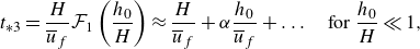 \begin{equation} t_{*3} = \frac {H}{\overline {u}_{{f}}} \mathcal{F}_1 \left ( \frac {h_0}{H} \right ) \approx \frac {H}{\overline {u}_{{f}}} + \alpha \frac {h_0}{\overline {u}_{{f}}} + \ldots \quad \text{for}\ \frac {h_0}{H} \ll 1, \end{equation}
where $\mathcal{F}$
and
$\mathcal{F}$
and $\mathcal{F}_1$
are functions and
$\mathcal{F}_1$
are functions and $\alpha$
is a constant, indicating that a linear combination of upstream and obstacle-induced time scales may provide a parametrisation for
$\alpha$
is a constant, indicating that a linear combination of upstream and obstacle-induced time scales may provide a parametrisation for $t_{*3}$
. To determine
$t_{*3}$
. To determine $\alpha$
using experiments, a phenomenological definition was proposed for
$\alpha$
using experiments, a phenomenological definition was proposed for $t_{*3}$
, where
$t_{*3}$
, where $h_0/\overline {u}_{{f}}$
is considered as introducing a post-collision modification to the upstream time scale
$h_0/\overline {u}_{{f}}$
is considered as introducing a post-collision modification to the upstream time scale $t_{*1} = H/\overline {u}_{{f}}$
(similar to that used in modelling multiple length-scale problems in turbulent boundary layers; Hunt Reference Hunt and Puttock1988). In this definition, the increase of propagation time
$t_{*1} = H/\overline {u}_{{f}}$
(similar to that used in modelling multiple length-scale problems in turbulent boundary layers; Hunt Reference Hunt and Puttock1988). In this definition, the increase of propagation time $\delta t$
compared with the propagation time without the obstacle
$\delta t$
compared with the propagation time without the obstacle $t_{*1}$
during stages II and III was considered as the perturbation time, and hence
$t_{*1}$
during stages II and III was considered as the perturbation time, and hence $t_{*3} = t_{*1} + \delta t$
in concurrence with (5.1). In so evaluating
$t_{*3} = t_{*1} + \delta t$
in concurrence with (5.1). In so evaluating $\delta t$
, it is necessary to know the downstream distance
$\delta t$
, it is necessary to know the downstream distance $x_3$
to which stage III persists, which is determined by the recirculation cell length after which the gravity current returns to its upstream velocity.
$x_3$
to which stage III persists, which is determined by the recirculation cell length after which the gravity current returns to its upstream velocity.
The conditions above the barrier at the start of stage II are the modified gravity current speed $\overline {u}_{{f},0}$
, depth of spillover of the gravity current
$\overline {u}_{{f},0}$
, depth of spillover of the gravity current $d_0$
and the local reduced gravity
$d_0$
and the local reduced gravity $g'$
. Thus, it is possible to write
$g'$
. Thus, it is possible to write
 \begin{equation} \frac {x_3}{H} = \mathcal{F}_2 (\overline {u}_{{f},0}, g', h_0, d_0, H) = \mathcal{F}_3 \left ( Fr_{d_0}, \frac {d_0}{H}, \frac {h_0}{H} \right ), \end{equation}
where $Fr_{d_0} = \overline {u}_{{f},0}/\sqrt {g' d_0}$
is the Froude number at the obstacle (
$Fr_{d_0} = \overline {u}_{{f},0}/\sqrt {g' d_0}$
is the Froude number at the obstacle ( $x = 0$
). For the cases presented, the data indicate that
$x = 0$
). For the cases presented, the data indicate that $x_3/H$
is roughly constant (not shown) independent of
$x_3/H$
is roughly constant (not shown) independent of $Fr_{d_0}$
and
$Fr_{d_0}$
and $d_0/H$
, and only slightly decreasing for the largest obstacle possibly due to hydraulic adjustment at the obstacle (e.g. Farmer & Armi Reference Farmer and Armi1986). Since the influence of
$d_0/H$
, and only slightly decreasing for the largest obstacle possibly due to hydraulic adjustment at the obstacle (e.g. Farmer & Armi Reference Farmer and Armi1986). Since the influence of $h_0/H$
could not be discounted unequivocally based on the (limited) data available,
$h_0/H$
could not be discounted unequivocally based on the (limited) data available, $x_3$
was estimated directly from the data rather than via a parametrisation such as (5.2). The increase of propagation time
$x_3$
was estimated directly from the data rather than via a parametrisation such as (5.2). The increase of propagation time $\delta t$
during stages II and III compared with the base case was evaluated as
$\delta t$
during stages II and III compared with the base case was evaluated as
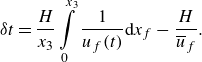 \begin{equation} \delta t = \frac {H}{x_3} \int \limits _0^{x_3} \frac {1}{u_{{f}}(t)} \mathrm{d}x_{{f}} - \frac {H}{\overline {u}_{{f}}}. \end{equation}
The resulting $\delta t$
are plotted in figure 5 as a function of
$\delta t$
are plotted in figure 5 as a function of $h_0/\overline {u}_{{f}}$
. The results show that
$h_0/\overline {u}_{{f}}$
. The results show that
 \begin{equation} \delta t = \alpha \frac {h_0}{\overline {u}_{{f}}} \end{equation}
with proportionality constant $\alpha = 4.5 \pm 1.0$
, which is strictly applicable for the range
$\alpha = 4.5 \pm 1.0$
, which is strictly applicable for the range $0 \leqslant h_0/2{h_{{g}}} \leqslant 0.3$
. Note that for larger
$0 \leqslant h_0/2{h_{{g}}} \leqslant 0.3$
. Note that for larger $h_0/2{h_{{g}}}$
, the flow over the obstacle is hydraulically impacted by a larger return flow and obstacles with
$h_0/2{h_{{g}}}$
, the flow over the obstacle is hydraulically impacted by a larger return flow and obstacles with $h_0/2{h_{{g}}} \sim 1$
realistically obstruct the entire gravity current (Lane-Serff et al. Reference Lane-Serff, Beal and Hadfield1995; Skevington & Hogg Reference Skevington and Hogg2023). Furthermore, for large obstacles, upstream propagating wave modes become important and the hydraulic adjustments upstream and at the barrier become complex (Janowitz Reference Janowitz1973). Thus, it is possible to propose, for stages II and III with
$h_0/2{h_{{g}}} \sim 1$
realistically obstruct the entire gravity current (Lane-Serff et al. Reference Lane-Serff, Beal and Hadfield1995; Skevington & Hogg Reference Skevington and Hogg2023). Furthermore, for large obstacles, upstream propagating wave modes become important and the hydraulic adjustments upstream and at the barrier become complex (Janowitz Reference Janowitz1973). Thus, it is possible to propose, for stages II and III with $0 \leqslant h_0/2{h_{{g}}} \leqslant 0.3$
,
$0 \leqslant h_0/2{h_{{g}}} \leqslant 0.3$
,
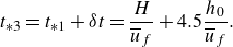 \begin{equation} t_{*3} = t_{*1} + \delta t = \frac {H}{\overline {u}_{{f}}} + 4.5 \frac {h_0}{\overline {u}_{{f}}}. \end{equation}
Figure 4(c,d) shows the normalised front position and speed against time normalised by time scale $t_{*3}$
. As expected,
$t_{*3}$
. As expected, $t_{*3}$
scaling fails in the pre-collision phase (stage I), but predicts stage II and III satisfactorily. This allows a quantitative identification of the start and end times of the four stages that characterise the collision of a gravity current with an obstacle, which are summarised below:
$t_{*3}$
scaling fails in the pre-collision phase (stage I), but predicts stage II and III satisfactorily. This allows a quantitative identification of the start and end times of the four stages that characterise the collision of a gravity current with an obstacle, which are summarised below:
Duration of reduced velocities during the collision (lag) as a function of $h_0/\overline {u}_{{f}}$
.
$h_0/\overline {u}_{{f}}$
.

Stage I ( $t/t_{*3}\lt -0.05$
). This is the slumping phase, where the gravity current approaches the obstacle with an approximately constant velocity (see figure 4
b). The slowdown begins just prior to making contact with the obstacle, which is the onset of stage II.
$t/t_{*3}\lt -0.05$
). This is the slumping phase, where the gravity current approaches the obstacle with an approximately constant velocity (see figure 4
b). The slowdown begins just prior to making contact with the obstacle, which is the onset of stage II.
Stage II ( $-0.05 \lt t/t_{*3} \lt 0.4$
). Upon contact with the obstacle, the gravity current is deflected upwards, drastically reducing the front velocity and converting a portion of the gravity current’s kinetic energy into potential energy (Wu & Ouyang Reference Wu and Ouyang2020). The hydraulic adjustment over the obstacle shrinks its thickness and increases the speed immediately downstream, which undergoes instabilities on either side of the current. Due to the noisy signal in figure 4, it is not entirely clear when the minimum front velocity is reached, but individual
$-0.05 \lt t/t_{*3} \lt 0.4$
). Upon contact with the obstacle, the gravity current is deflected upwards, drastically reducing the front velocity and converting a portion of the gravity current’s kinetic energy into potential energy (Wu & Ouyang Reference Wu and Ouyang2020). The hydraulic adjustment over the obstacle shrinks its thickness and increases the speed immediately downstream, which undergoes instabilities on either side of the current. Due to the noisy signal in figure 4, it is not entirely clear when the minimum front velocity is reached, but individual $\overline {\rho }$
fields confirm that gravity current reaches its maximum height at
$\overline {\rho }$
fields confirm that gravity current reaches its maximum height at $t/t_{*3} \approx 0.4$
and collapses thereafter.
$t/t_{*3} \approx 0.4$
and collapses thereafter.
Stage III ( $0.4 \lt t/t_{*3} \lt 0.75$
). The lofted gravity current descends (collapses), converting the potential energy back into kinetic energy, leading to an increased front speed. Stage III concludes as the front velocity approaches
$0.4 \lt t/t_{*3} \lt 0.75$
). The lofted gravity current descends (collapses), converting the potential energy back into kinetic energy, leading to an increased front speed. Stage III concludes as the front velocity approaches $\overline {u}_{{f}}$
, although the exact final value for some cases is obscured by the gravity current exiting the measurement window.
$\overline {u}_{{f}}$
, although the exact final value for some cases is obscured by the gravity current exiting the measurement window.
Stage IV ( $t/t_{*3} \gt 0.75$
). After reattaching to the bottom surface, the gravity current continues its propagation out of the field of view at a speed close to
$t/t_{*3} \gt 0.75$
). After reattaching to the bottom surface, the gravity current continues its propagation out of the field of view at a speed close to $\overline {u}_{{f}}$
. A recirculation zone persists behind the obstacle.
$\overline {u}_{{f}}$
. A recirculation zone persists behind the obstacle.
Blocking effect of the obstacle. (a) Gravity current thickness and (b) mass flux of the gravity current at $x = 0$
. The solid and dashed lines are for the lower and higher
$x = 0$
. The solid and dashed lines are for the lower and higher $Re$
cases, respectively.
$Re$
cases, respectively.

5.2. Blocking effect of the obstacle
In addition to reducing the horizontal motion of the gravity current, the obstacle exerts a ‘blocking’ effect that manifests as a reflected hydraulic jump. Key parameters in this context are the ‘thickness’ of the gravity current $d(t)$
as well as the mass flux (per unit width)
$d(t)$
as well as the mass flux (per unit width) $M(t)$
of the gravity current over the obstacle (at
$M(t)$
of the gravity current over the obstacle (at $x = 0$
). The gravity current thickness over the obstacle is calculated as
$x = 0$
). The gravity current thickness over the obstacle is calculated as
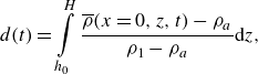 \begin{equation} d(t) = \int \limits _{h_0}^H \frac {\overline {\rho }(x=0,z,t) - \rho _{{a}}}{\rho _1 - \rho _{{a}}} \mathrm{d}z, \end{equation}
and the mass flux $M(t)$
is defined as
$M(t)$
is defined as
 \begin{equation} M(t) = \int _{h_0}^{h_0 + d(t)} \overline {\rho }(x=0,z,t)\overline {u}(x=0,z,t) \mathrm{d}z \approx \rho _0 \int _{h_0}^{h_0 + d(t)} \overline {u}(x=0,z,t) \mathrm{d}z. \end{equation}
Figure 6 presents the evolution of $d(t)$
and
$d(t)$
and $M(t)$
. Note that
$M(t)$
. Note that $d(t)$
becomes non-zero when the nose of the gravity current touches the obstacle at
$d(t)$
becomes non-zero when the nose of the gravity current touches the obstacle at $t \approx 0$
and spills over the barrier. This thickness
$t \approx 0$
and spills over the barrier. This thickness $d(t)$
increases over time as the head and body of the gravity current pass over the obstacle, reaching a peak at
$d(t)$
increases over time as the head and body of the gravity current pass over the obstacle, reaching a peak at $t/t_{*1} \approx 1$
, and then decrease approximately linearly thereafter. The thickness appears to be mostly independent of the obstacle height, with a maximum of
$t/t_{*1} \approx 1$
, and then decrease approximately linearly thereafter. The thickness appears to be mostly independent of the obstacle height, with a maximum of $d = 0.47H$
, which is approximately equal to the height of an undisturbed gravity current
$d = 0.47H$
, which is approximately equal to the height of an undisturbed gravity current ${h_{{g}}} = 0.5H$
(Benjamin Reference Benjamin1968). Note that
${h_{{g}}} = 0.5H$
(Benjamin Reference Benjamin1968). Note that $t_{*1}$
, and not
$t_{*1}$
, and not $t_{*3}$
, appears to be the appropriate time scale for
$t_{*3}$
, appears to be the appropriate time scale for $d(t)$
because of an unpropitious collapse of the curves with
$d(t)$
because of an unpropitious collapse of the curves with $t_{*3}$
, perhaps because the obstacle effect (quantified by
$t_{*3}$
, perhaps because the obstacle effect (quantified by $\delta t$
) only comes into play downstream of the obstacle.
$\delta t$
) only comes into play downstream of the obstacle.
For the unobstructed case, the mass flux follows a trend similar to $d(t)$
, but enhanced variations appear in the obstructed cases. The maximum of
$d(t)$
, but enhanced variations appear in the obstructed cases. The maximum of $M(t)$
decreases with increasing obstacle height and occurs later in time. The collapse of the different curves is insufficient for both
$M(t)$
decreases with increasing obstacle height and occurs later in time. The collapse of the different curves is insufficient for both $t_{*1}$
and
$t_{*1}$
and $t_{*3}$
(not shown), indicating a more complex adjustment of
$t_{*3}$
(not shown), indicating a more complex adjustment of $M(t)$
at the obstruction. As depicted in figure 3(b1), immediately after the gravity current makes contact with the obstacle, its upper portion is reflected back upstream, effectively reducing the mass flux over the obstacle. Then, the gravity current accelerates as it moves past the obstacle, as shown in figure 3(c3). Additionally, oscillations of
$M(t)$
at the obstruction. As depicted in figure 3(b1), immediately after the gravity current makes contact with the obstacle, its upper portion is reflected back upstream, effectively reducing the mass flux over the obstacle. Then, the gravity current accelerates as it moves past the obstacle, as shown in figure 3(c3). Additionally, oscillations of $M(t)$
are clear from figure 6(b), which are possibly due to the excitation of wave modes at the obstacle with a frequency determined by the gravity-current/obstacle interaction (e.g. Houcine et al. Reference Houcine, Chashechkin, Fraunie, Fernando, Gharbi and Lili2012). The frequency of the oscillations was compared with various theoretical expressions for interfacial waves, KH instabilities, propagating lee waves, standing surface waves and internal waves (for a discussion on these modes, see Turner Reference Turner1973), but no good agreement could be found. The unsteady nature of gravity-current/obstacle interactions studied here appears to introduce additional complexities that are intractable by available theoretical formulations.
$M(t)$
are clear from figure 6(b), which are possibly due to the excitation of wave modes at the obstacle with a frequency determined by the gravity-current/obstacle interaction (e.g. Houcine et al. Reference Houcine, Chashechkin, Fraunie, Fernando, Gharbi and Lili2012). The frequency of the oscillations was compared with various theoretical expressions for interfacial waves, KH instabilities, propagating lee waves, standing surface waves and internal waves (for a discussion on these modes, see Turner Reference Turner1973), but no good agreement could be found. The unsteady nature of gravity-current/obstacle interactions studied here appears to introduce additional complexities that are intractable by available theoretical formulations.
6. Evolution of turbulent kinetic energy
To estimate the turbulent kinetic energy (TKE) fields in the proximity of the obstacle, the ensemble-averaged velocity was subtracted from the individual velocity-field realisations, and the squared fluctuations were subsequently averaged. For consistency, the focus is on spatially averaged TKE values. Averaging TKE over the entire domain may not provide accurate insights, as it is influenced by both local turbulence characteristics as well as the progression of the gravity current. As such, TKE was computed over two specific domains. The primary domain was a ‘dynamic box’ aligned with the gravity-current’s front ( $x_{{f}}(t) - 0.5H \lt x \lt x_{{f}}(t)$
,
$x_{{f}}(t) - 0.5H \lt x \lt x_{{f}}(t)$
, $0 \lt z \lt H$
). The TKE (or turbulence intensity) averaged within this frontal box is defined as
$0 \lt z \lt H$
). The TKE (or turbulence intensity) averaged within this frontal box is defined as
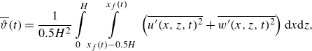 \begin{align} \overline {\vartheta }(t) & = \frac {1}{0.5H^2} \int \limits _0^H \int \limits _{x_{{f}}(t)-0.5H}^{x_{{f}}(t)} \left ( \overline {u'(x,z,t)^2} + \overline {w'(x,z,t)^2} \right ) \mathrm{d}x \mathrm{d}z, \end{align}
 \begin{align} \overline {T}(t) & = \frac {\overline {\vartheta }(t)}{\overline {u}_{{f}}^2}, \end{align}
where $u'$
and
$u'$
and $w'$
denote horizontal and vertical velocity fluctuations, and
$w'$
denote horizontal and vertical velocity fluctuations, and $\overline {\vartheta }$
and
$\overline {\vartheta }$
and $\overline {T}$
represent the dimensional and dimensionless TKE within the frontal box. The spanwise velocity component is not factored into (6.1) as it was not measured; nonetheless,
$\overline {T}$
represent the dimensional and dimensionless TKE within the frontal box. The spanwise velocity component is not factored into (6.1) as it was not measured; nonetheless, $\overline {\vartheta }$
and
$\overline {\vartheta }$
and $\overline {T}$
serve as proxies for the TKE.
$\overline {T}$
serve as proxies for the TKE.
Figure 7(a) displays $\overline {T}$
for all cases. The normalised TKE for the unobstructed cases (in blue) remained roughly constant over time. In obstructed cases, during the approach phase (stage I), the TKE also remained constant. As the gravity current started interacting with the obstacle and deflected upward (stage II),
$\overline {T}$
for all cases. The normalised TKE for the unobstructed cases (in blue) remained roughly constant over time. In obstructed cases, during the approach phase (stage I), the TKE also remained constant. As the gravity current started interacting with the obstacle and deflected upward (stage II), $\overline {T}$
continued to remain constant and did not yet increase despite the formation of a recirculation vortex beneath the gravity-current nose, possibly due to the time delay required for instabilities to set in and generate TKE. Once the gravity current reached its peak height and collapsed (stage III),
$\overline {T}$
continued to remain constant and did not yet increase despite the formation of a recirculation vortex beneath the gravity-current nose, possibly due to the time delay required for instabilities to set in and generate TKE. Once the gravity current reached its peak height and collapsed (stage III), $\overline {T}$
increased due to the generation of turbulence at the top and bottom boundaries of the gravity current head. The normalised TKE appears to peak at
$\overline {T}$
increased due to the generation of turbulence at the top and bottom boundaries of the gravity current head. The normalised TKE appears to peak at $t/t_{*3} \approx 0.75$
, although the data beyond are mostly unavailable as it is outside the probing volume. The inset in figure 7(a) illustrates the maximum value of
$t/t_{*3} \approx 0.75$
, although the data beyond are mostly unavailable as it is outside the probing volume. The inset in figure 7(a) illustrates the maximum value of $\overline {T}$
for each case as a function of the normalised obstacle height
$\overline {T}$
for each case as a function of the normalised obstacle height $h_0/2{h_{{g}}}$
, demonstrating its influence on local TKE generation via flow separation. The maximum
$h_0/2{h_{{g}}}$
, demonstrating its influence on local TKE generation via flow separation. The maximum $\overline {T}$
appears to be independent of the Reynolds number.
$\overline {T}$
appears to be independent of the Reynolds number.
Evolution of the dimensionless TKE. (a) Averaged TKE, $\overline {T}(t)$
, in the frontal region for all cases. The solid and dashed lines are for the lower and higher
$\overline {T}(t)$
, in the frontal region for all cases. The solid and dashed lines are for the lower and higher $Re$
cases, respectively, and the colours correspond to those of figure 6. The inset shows the maximum values as a function of the obstacle height for the two
$Re$
cases, respectively, and the colours correspond to those of figure 6. The inset shows the maximum values as a function of the obstacle height for the two $Re$
values, with
$Re$
values, with $\overline {T}_{{max}} = 0.44h_0/2{h_{{g}}} + 0.038$
. (b) Averaged TKE,
$\overline {T}_{{max}} = 0.44h_0/2{h_{{g}}} + 0.038$
. (b) Averaged TKE, $\overline {T}(z,t)$
, for the C5200H0.1 case including vertical variations, defined in (6.2).
$\overline {T}(z,t)$
, for the C5200H0.1 case including vertical variations, defined in (6.2).
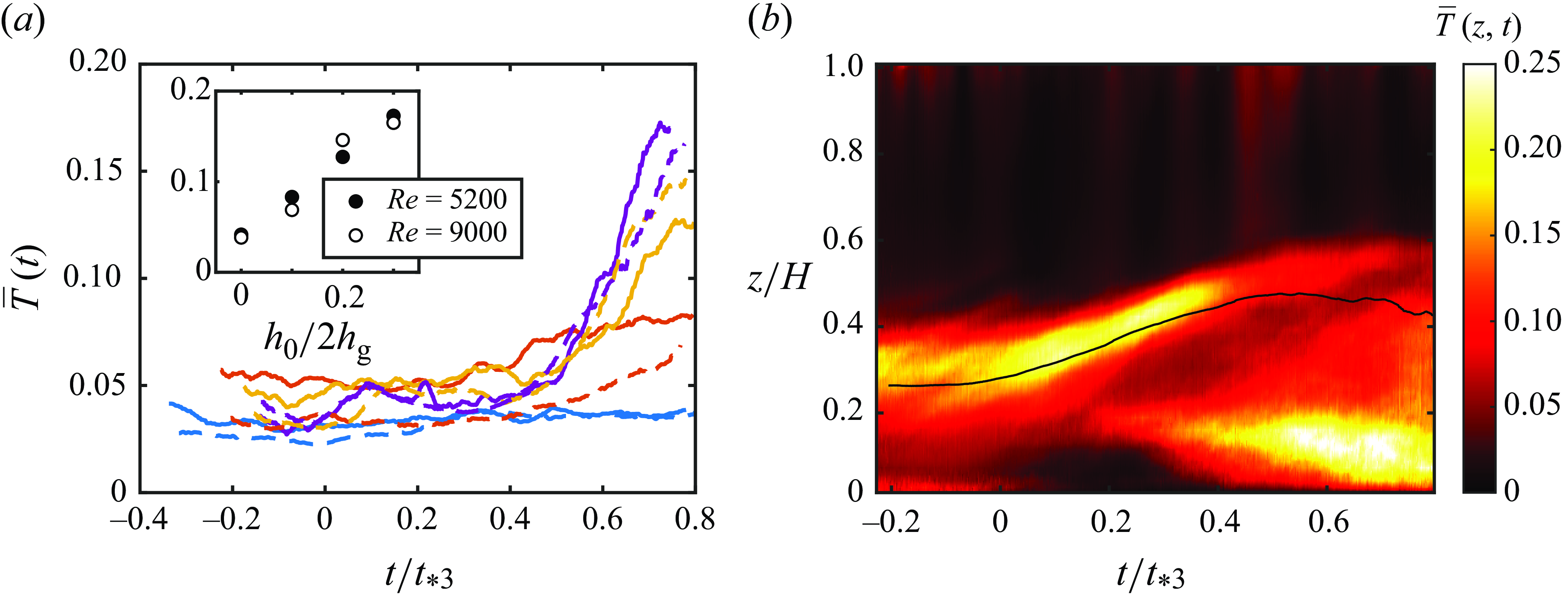
Spatial averaging as in (6.1) does not capture key spatial variations, and to this end, a more suitable quantity that includes vertical variations was considered (Zhong et al. Reference Zhong, Hussain and Fernando2018):
 \begin{align} \overline {\vartheta }(z,t) & = \frac {1}{0.5H} \int \limits _{x_{{f}}(t)-0.5H}^{x_{{f}}(t)} \left ( \overline {u'(x,z,t)^2} + \overline {z'(x,z,t)^2} \right ) \mathrm{d}x, \end{align}
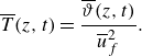 \begin{align} \overline {T}(z,t) & = \frac {\overline {\vartheta }(z,t)}{\overline {u}_{{f}}^2}. \end{align}
Figure 7(b) presents $\overline {T}(z,t)$
at various heights and times for the C5200H0.1 case. The black line indicates the averaged gravity-current height within the frontal box, as determined from the
$\overline {T}(z,t)$
at various heights and times for the C5200H0.1 case. The black line indicates the averaged gravity-current height within the frontal box, as determined from the $\overline {\rho } = (\rho _1 + \rho _{{a}})/2$
contour. Prior to the collision (stage I), most turbulence was observed in the shear layer atop the gravity current (see figure 3
a3). During stage II, the turbulence in the shear layer was concentrated in a narrower region, but beyond
$\overline {\rho } = (\rho _1 + \rho _{{a}})/2$
contour. Prior to the collision (stage I), most turbulence was observed in the shear layer atop the gravity current (see figure 3
a3). During stage II, the turbulence in the shear layer was concentrated in a narrower region, but beyond $t/t_{*3} = 0.4$
, TKE diminished, likely due to the collapse/descend (start of stage III) of the gravity current, as evident from figure 4(d). At
$t/t_{*3} = 0.4$
, TKE diminished, likely due to the collapse/descend (start of stage III) of the gravity current, as evident from figure 4(d). At $t/t_{*3} = 0.2$
, a vortex was generated under the gravity-current head, leading to the production of a small amount of TKE in this region. Nevertheless, the total TKE remained constant during stage II (figure 7
a). After
$t/t_{*3} = 0.2$
, a vortex was generated under the gravity-current head, leading to the production of a small amount of TKE in this region. Nevertheless, the total TKE remained constant during stage II (figure 7
a). After $t/t_{*3} = 0.4$
, the gravity current sped downward, generating instabilities in the shear layers at both the top and bottom edges of the gravity current (e.g. figure 2
c). The bottom boundary of the current exhibited vigorous RT instabilities owing to the unstable stratification. This combination of shear and unstable stratification resulted in a significant increase in turbulence at the bottom region of the gravity current front (figure 7
b), whereas the top region exhibited less turbulence.
$t/t_{*3} = 0.4$
, the gravity current sped downward, generating instabilities in the shear layers at both the top and bottom edges of the gravity current (e.g. figure 2
c). The bottom boundary of the current exhibited vigorous RT instabilities owing to the unstable stratification. This combination of shear and unstable stratification resulted in a significant increase in turbulence at the bottom region of the gravity current front (figure 7
b), whereas the top region exhibited less turbulence.
Figure 8(a) displays $\overline {T}(t)$
, now averaged over the obstacle lee (
$\overline {T}(t)$
, now averaged over the obstacle lee ( $x \gt 0$
), with normalised shifted time
$x \gt 0$
), with normalised shifted time $(t-t_{{max}})/t_{*3}$
, where
$(t-t_{{max}})/t_{*3}$
, where $t_{{max}}$
is the time where
$t_{{max}}$
is the time where $\overline {T}$
acquires its maximum value in the obstacle lee. The time
$\overline {T}$
acquires its maximum value in the obstacle lee. The time $t_{{max}}/t_{*3}$
is approximately constant, having an average value of
$t_{{max}}/t_{*3}$
is approximately constant, having an average value of $1.2 \pm 0.2$
. Note that this is different from the frontal box studied in figure 7, which reaches a maximum value of
$1.2 \pm 0.2$
. Note that this is different from the frontal box studied in figure 7, which reaches a maximum value of $\overline {T}$
sooner, since it covers a different domain. Figure 8 shows that
$\overline {T}$
sooner, since it covers a different domain. Figure 8 shows that $\overline {T}(t)$
in the obstacle lee asymptotically approaches to that of an unobstructed gravity current over a time of
$\overline {T}(t)$
in the obstacle lee asymptotically approaches to that of an unobstructed gravity current over a time of $t/t_{*3} \approx 0.8$
. The vertical distribution of
$t/t_{*3} \approx 0.8$
. The vertical distribution of $\overline {T}(z,t)$
in the obstacle lee is given in figure 8(b), indicating that initial vertical mixing is intense over the entire gravity current column, but after attaining a maximum, the highest TKE regions are in the outer shear layer and the wall bounded shear layer, similar to the unobstructed case.
$\overline {T}(z,t)$
in the obstacle lee is given in figure 8(b), indicating that initial vertical mixing is intense over the entire gravity current column, but after attaining a maximum, the highest TKE regions are in the outer shear layer and the wall bounded shear layer, similar to the unobstructed case.
Evolution of the average turbulence kinetic energy in the (a) downstream region for all cases and (b) C5200H0.1 case including vertical variations. The solid and dashed lines are for the lower and higher $Re$
cases, respectively. The maximum normalised TKE is reached at a time
$Re$
cases, respectively. The maximum normalised TKE is reached at a time $t_{{max}}/t_{*3}$
, which has an average value of
$t_{{max}}/t_{*3}$
, which has an average value of $1.2 \pm 0.2$
.
$1.2 \pm 0.2$
.
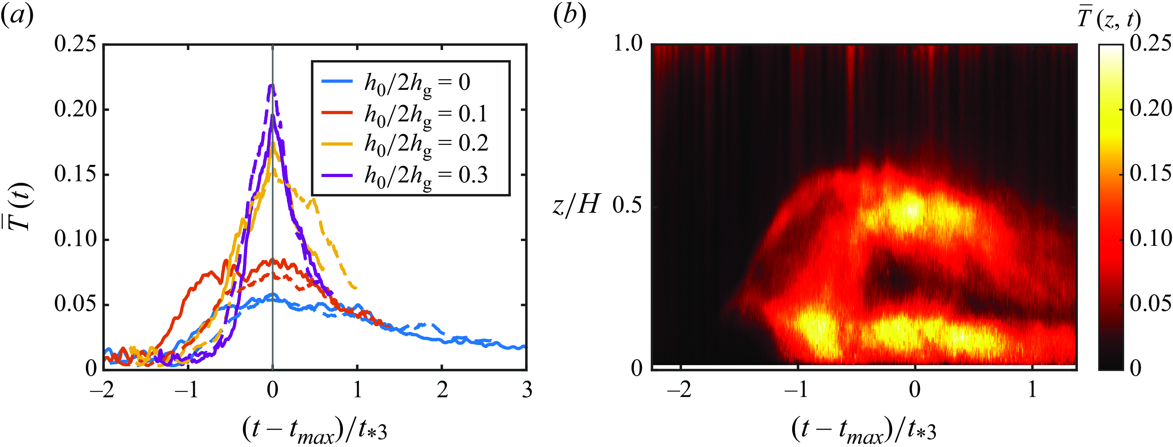
A referee noted the disparity between the onset of TKE increase in our case and those of Zhong, Hussain & Fernando (Reference Zhong, Hussain and Fernando2018, laboratory experiments) and Dai, Huang & Wu (Reference Dai, Huang and Wu2023, direct numerical simulations) where the collision of two identical counterflowing gravity currents was studied. In our case, during stage II, the TKE remains approximately constant until $t/t_{*3} \approx 0.2$
, and then shows a slow rise in
$t/t_{*3} \approx 0.2$
, and then shows a slow rise in $0.2 \lt t/t_{*3} \lt 0.4$
(figure 7
a). Close inspection shows that during
$0.2 \lt t/t_{*3} \lt 0.4$
(figure 7
a). Close inspection shows that during $-0.05 \lt t/t_{*3} \lt 0.2$
, most of the TKE (production) is concentrated in the top shear layer where the production and dissipation appear to balance, and with time, the TKE in the shear layer reduces gradually (figure 7
b). At
$-0.05 \lt t/t_{*3} \lt 0.2$
, most of the TKE (production) is concentrated in the top shear layer where the production and dissipation appear to balance, and with time, the TKE in the shear layer reduces gradually (figure 7
b). At $t/t_{*3} = 0.28$
(or
$t/t_{*3} = 0.28$
(or $t/t_{*1} \approx 0.4$
), a vortex forms below the separating shear layer above the barrier and compensates for the reduction of TKE in the approaching shear layer, thus causing maintenance or a slow increase of TKE in the frontal domain. Breakdown of shear layers of the overtopping flow and lee vortex is responsible for the rapid increase of TKE at
$t/t_{*1} \approx 0.4$
), a vortex forms below the separating shear layer above the barrier and compensates for the reduction of TKE in the approaching shear layer, thus causing maintenance or a slow increase of TKE in the frontal domain. Breakdown of shear layers of the overtopping flow and lee vortex is responsible for the rapid increase of TKE at $t/t_{*3} \gt 0.4$
(equivalent to
$t/t_{*3} \gt 0.4$
(equivalent to $t/t_{*1} \approx 0.6$
in figure 2). In the case of two colliding gravity currents, flow structures at the impingement region are different (cf. figures 2, 3 in the present paper, figures 2 and 3 of Zhong et al. (Reference Zhong, Hussain and Fernando2018), and figures 2 and 3 of Dai et al. Reference Dai, Huang and Wu2023), and there is no vortex-induced TKE production. Zhong et al. (Reference Zhong, Hussain and Fernando2018)observed that the maximum TKE occurs at
$t/t_{*1} \approx 0.6$
in figure 2). In the case of two colliding gravity currents, flow structures at the impingement region are different (cf. figures 2, 3 in the present paper, figures 2 and 3 of Zhong et al. (Reference Zhong, Hussain and Fernando2018), and figures 2 and 3 of Dai et al. Reference Dai, Huang and Wu2023), and there is no vortex-induced TKE production. Zhong et al. (Reference Zhong, Hussain and Fernando2018)observed that the maximum TKE occurs at $-0.2 \lt t \overline {u}_{{f}}/H \lt 0.2$
, which is due to modifications of the shear layer in the gravity-current top due to collisions. Hence, in the two-current collision case, the TKE increase occurs immediately after the collision, and the domain averaged maximum TKE levels (
$-0.2 \lt t \overline {u}_{{f}}/H \lt 0.2$
, which is due to modifications of the shear layer in the gravity-current top due to collisions. Hence, in the two-current collision case, the TKE increase occurs immediately after the collision, and the domain averaged maximum TKE levels ( $\overline {T} \sim 0.06 {-} 0.08$
) are smaller than in the case with a solid wall, where
$\overline {T} \sim 0.06 {-} 0.08$
) are smaller than in the case with a solid wall, where $\overline {T} \sim 0.1$
–0.15 occurs during the vortex formation, later in the flow development.
$\overline {T} \sim 0.1$
–0.15 occurs during the vortex formation, later in the flow development.
7. Turbulent mixing
7.1. Rate of change of buoyancy
The collision of the gravity current with the obstacle leads to the development of instabilities over and downstream of the obstacle (see figure 2 c,d), resulting in mixing and homogenisation of the gravity current and ambient fluids. The time rate of change of buoyancy of a fluid parcel can be calculated as follows (Zhong et al. Reference Zhong, Hussain and Fernando2018):
 \begin{equation} \frac {\mathrm{D}b}{\mathrm{D}t}(x,z,t) = \frac {b(x + u(x,z,t) \Delta t,z + w(x,z,t) \Delta t,t + \Delta t) - b(x,z,t)}{\Delta t}, \end{equation}
where $\Delta t$
is the time interval between two image frames. This formulation assumes in-plane flow, which is a reasonable approximation given that the measurements were in the centre plane of the tank, where
$\Delta t$
is the time interval between two image frames. This formulation assumes in-plane flow, which is a reasonable approximation given that the measurements were in the centre plane of the tank, where $\overline {v} \approx 0$
.
$\overline {v} \approx 0$
.
Figure 9(a,b) presents the normalised buoyancy fields at two instances of C5200H0.1 following the collision, and figure 9(c,d) depicts the corresponding $Db/Dt$
fields, calculated using (7.1). At
$Db/Dt$
fields, calculated using (7.1). At $t/t_{*3} \approx 0.2$
, a vortex started to form beneath the gravity-current head, exhibiting significant
$t/t_{*3} \approx 0.2$
, a vortex started to form beneath the gravity-current head, exhibiting significant $\mathrm{D}b/\mathrm{D}t$
values and contributing significantly to mixing in stages II and III. As the gravity current collapsed in stage III, mixing primarily occurred at the top and bottom shear layers, where KH and RT instabilities developed (figure 9
b), as discussed in § 6, and instabilities at the lower edge of the current were pronounced and
$\mathrm{D}b/\mathrm{D}t$
values and contributing significantly to mixing in stages II and III. As the gravity current collapsed in stage III, mixing primarily occurred at the top and bottom shear layers, where KH and RT instabilities developed (figure 9
b), as discussed in § 6, and instabilities at the lower edge of the current were pronounced and $\mathrm{D}b/\mathrm{D}t$
was more vigorous.
$\mathrm{D}b/\mathrm{D}t$
was more vigorous.
Two instances of the (a,b) buoyancy and (c,d) $\mathrm{D}b/\mathrm{D}t$
fields for C5200H0.1.
$\mathrm{D}b/\mathrm{D}t$
fields for C5200H0.1.
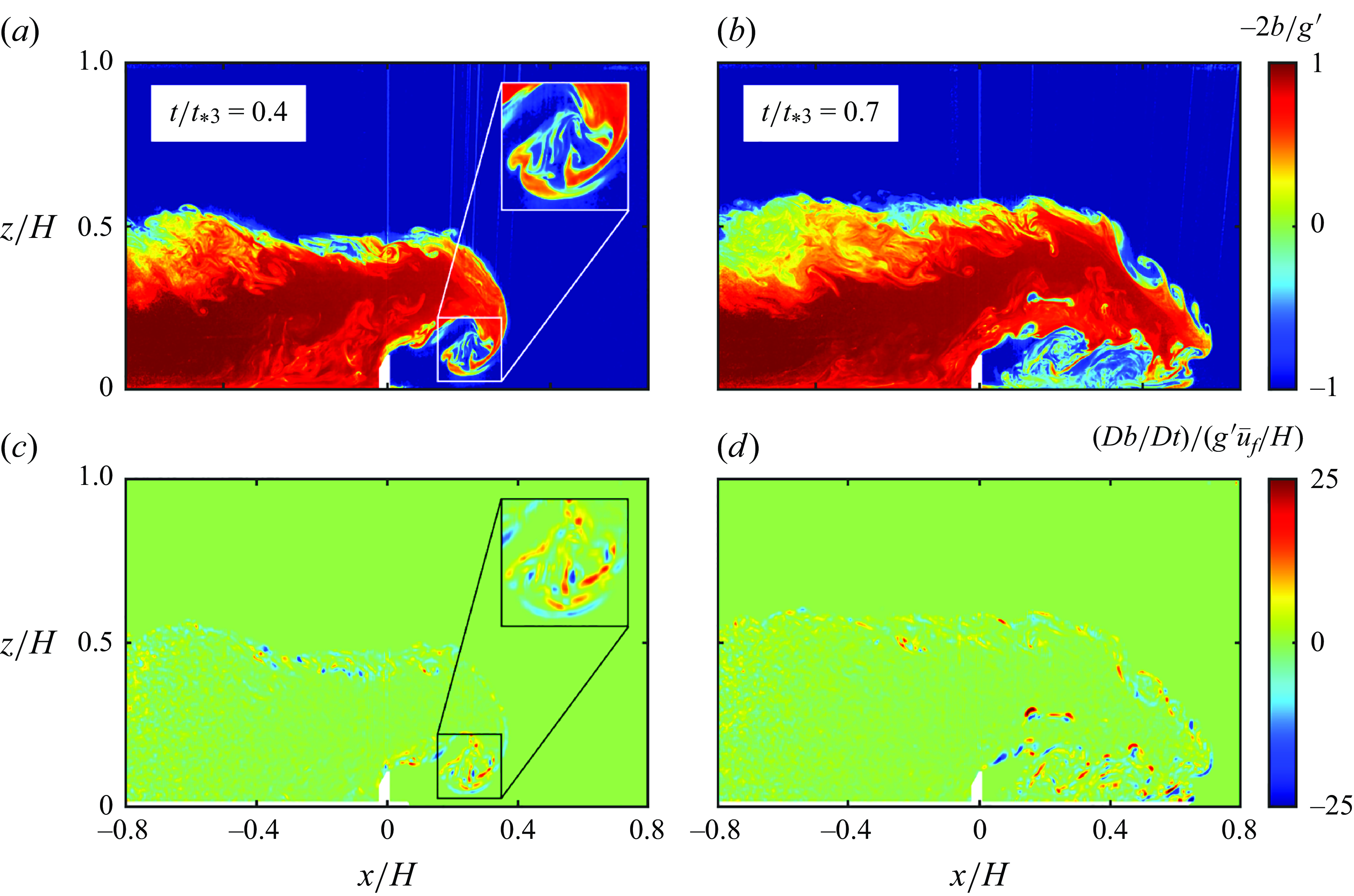
Similar to (6.1) and (6.2), the spatially averaged rate of change of mean buoyancy in the gravity-current front is defined as
 \begin{equation} \overline {\frac {\mathrm{D}b}{\mathrm{D}t}}(t) = \frac {1}{0.5H^2} \int \limits _0^H \int \limits _{x_{{f}}(t)-0.5H}^{x_{{f}}(t)} \left | \frac {\mathrm{D}\overline {b}}{\mathrm{D}t} \right | \mathrm{d}x \mathrm{d}z, \end{equation}
and to account for vertical variability:
 \begin{equation} \overline {\frac {\mathrm{D}b}{\mathrm{D}t}}(z,t) = \frac {1}{0.5H} \int \limits _{x_{{f}}(t)-0.5H}^{x_{{f}}(t)} \left | \frac {\mathrm{D}\overline {b}}{\mathrm{D}t} \right | \mathrm{d}x. \end{equation}
Here, $\mathrm{D}\overline {b}/\mathrm{D}t$
is obtained by applying (7.1) with averaged quantities instead of instantaneous ones. The use of the absolute value in
$\mathrm{D}\overline {b}/\mathrm{D}t$
is obtained by applying (7.1) with averaged quantities instead of instantaneous ones. The use of the absolute value in $\mathrm{D}\overline {b}/\mathrm{D}t$
is to account for positive and negative changes of buoyancy in turbulent mixing.
$\mathrm{D}\overline {b}/\mathrm{D}t$
is to account for positive and negative changes of buoyancy in turbulent mixing.
The evolution of $\overline {\mathrm{D}b/\mathrm{D}t}$
is shown in figure 10(a). Unobstructed gravity currents (blue line) exhibited an approximately constant value, indicative of a quasi-steady mixing rate. In the obstructed cases,
$\overline {\mathrm{D}b/\mathrm{D}t}$
is shown in figure 10(a). Unobstructed gravity currents (blue line) exhibited an approximately constant value, indicative of a quasi-steady mixing rate. In the obstructed cases, $\overline {\mathrm{D}b/\mathrm{D}t}$
remained constant before the collision (stage I), but increased following the collision (stage II) due to enhanced mixing. Immediately following the collision, mixing was higher at the top of the gravity current, however, by
$\overline {\mathrm{D}b/\mathrm{D}t}$
remained constant before the collision (stage I), but increased following the collision (stage II) due to enhanced mixing. Immediately following the collision, mixing was higher at the top of the gravity current, however, by $t/t_{*3} \approx 0.2$
, mixing intensified in the vortex and at the bottom of the gravity current (figure 10
b). In stage III,
$t/t_{*3} \approx 0.2$
, mixing intensified in the vortex and at the bottom of the gravity current (figure 10
b). In stage III, $\overline {\mathrm{D}b/\mathrm{D}t}$
stabilised for the smallest obstacle but continued to escalate for larger obstacles, peaking at
$\overline {\mathrm{D}b/\mathrm{D}t}$
stabilised for the smallest obstacle but continued to escalate for larger obstacles, peaking at $t/t_{*3} = 0.6$
. Additionally, differences in mixing emerge between various obstacle heights. Note that the maximum values of
$t/t_{*3} = 0.6$
. Additionally, differences in mixing emerge between various obstacle heights. Note that the maximum values of $\overline {\mathrm{D}b/\mathrm{D}t}$
are not influenced by the Reynolds number. The parallels between figures 7 and 10 highlight that turbulent mixing of buoyancy predominantly occurs in regions of high TKE.
$\overline {\mathrm{D}b/\mathrm{D}t}$
are not influenced by the Reynolds number. The parallels between figures 7 and 10 highlight that turbulent mixing of buoyancy predominantly occurs in regions of high TKE.
Evolution of $\overline {\mathrm{D}b/\mathrm{D}t}$
with time. (a) Spatially averaged
$\overline {\mathrm{D}b/\mathrm{D}t}$
with time. (a) Spatially averaged $\overline {\mathrm{D}b/\mathrm{D}t}$
fields in the frontal region for all cases. The solid and dashed lines are for the lower and higher
$\overline {\mathrm{D}b/\mathrm{D}t}$
fields in the frontal region for all cases. The solid and dashed lines are for the lower and higher $Re$
cases, respectively. The inset shows the maximum of
$Re$
cases, respectively. The inset shows the maximum of $\overline {\mathrm{D}b/\mathrm{D}t}$
as a function of the normalised obstacle height. (b) Horizontally averaged
$\overline {\mathrm{D}b/\mathrm{D}t}$
as a function of the normalised obstacle height. (b) Horizontally averaged $\overline {\mathrm{D}b/\mathrm{D}t}$
field for the C5200H0.2 case, as defined in (7.3). Different colours correspond to different
$\overline {\mathrm{D}b/\mathrm{D}t}$
field for the C5200H0.2 case, as defined in (7.3). Different colours correspond to different $h_0/2{h_{{g}}}$
, as shown in the inset of figure 8(a).
$h_0/2{h_{{g}}}$
, as shown in the inset of figure 8(a).
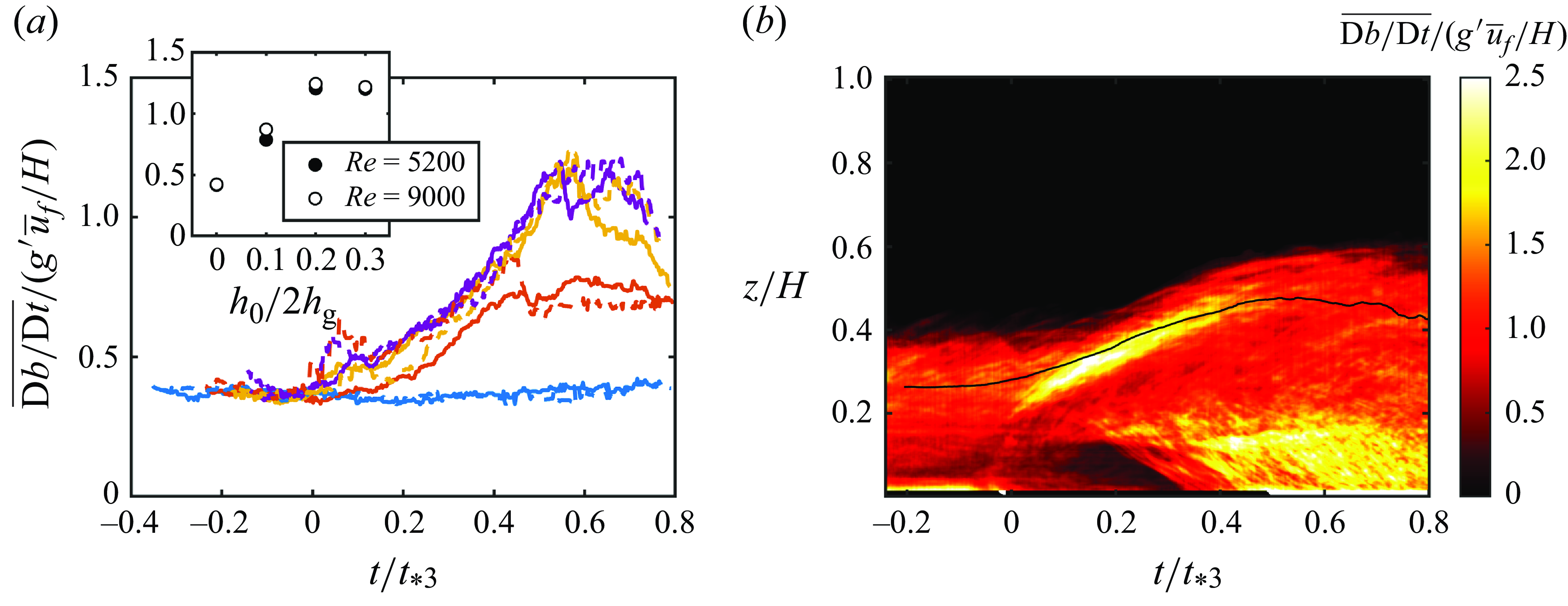
7.2. Eddy diffusivity
(a) Evolution of the spatially averaged eddy diffusivity. The solid and dashed lines are for the lower and higher $Re$
cases, respectively. (b) Horizontally averaged eddy diffusivity for the C5200H0.2 case. (c) Eddy diffusivities averaged over both space and time during stage III.
$Re$
cases, respectively. (b) Horizontally averaged eddy diffusivity for the C5200H0.2 case. (c) Eddy diffusivities averaged over both space and time during stage III.
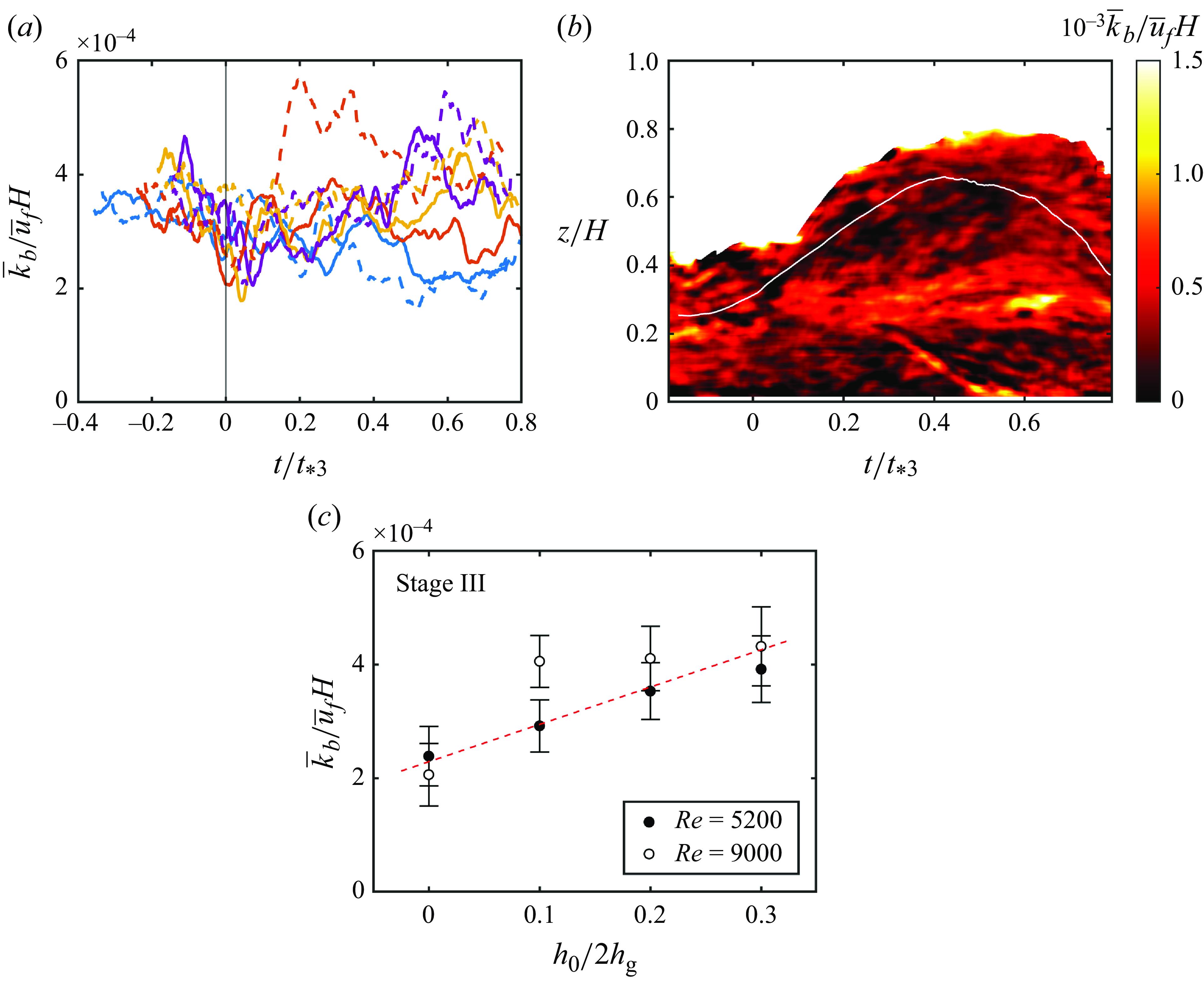
The eddy diffusivity $k_b$
was determined using the direct-evaluation approach of Zhong et al. (Reference Zhong, Hussain and Fernando2018), where velocity and buoyancy data at every point in space (
$k_b$
was determined using the direct-evaluation approach of Zhong et al. (Reference Zhong, Hussain and Fernando2018), where velocity and buoyancy data at every point in space ( $x$
,
$x$
, $z$
) and time were used to calculate
$z$
) and time were used to calculate
 \begin{equation} \frac {\mathrm{D}\overline {b}}{\mathrm{D}t} = k_b \nabla ^2 \overline {b}. \end{equation}
Before applying (7.4), the buoyancy fields were filtered by employing a 2-D moving average in space with a window size of $0.02H$
to ensure smooth derivatives. The central difference method was used for
$0.02H$
to ensure smooth derivatives. The central difference method was used for $\nabla ^2 \overline {b}$
, and the ratio of
$\nabla ^2 \overline {b}$
, and the ratio of $\mathrm{D}\overline {b}/\mathrm{D}t$
and
$\mathrm{D}\overline {b}/\mathrm{D}t$
and $\nabla ^2 \overline {b}$
yielded
$\nabla ^2 \overline {b}$
yielded $k_b$
. As noted by Zhong et al. (Reference Zhong, Hussain and Fernando2018), spurious
$k_b$
. As noted by Zhong et al. (Reference Zhong, Hussain and Fernando2018), spurious $k_b$
values in regions of nearly constant buoyancy were observed. To mitigate noise, values outside ten standard deviations from the mean were filtered out to obtain a refined
$k_b$
values in regions of nearly constant buoyancy were observed. To mitigate noise, values outside ten standard deviations from the mean were filtered out to obtain a refined $k_b$
distribution, from which the spatially averaged
$k_b$
distribution, from which the spatially averaged $\overline {k}_b$
was calculated. This averaging was performed over the ’frontal box’ (or gravity-current head) similar to that defined in (6.1).
$\overline {k}_b$
was calculated. This averaging was performed over the ’frontal box’ (or gravity-current head) similar to that defined in (6.1).
Figure 11(a) shows the temporal evolution of spatially averaged $\overline {k}_b$
in the gravity-current head. To enhance clarity, a moving-average filter has been applied to
$\overline {k}_b$
in the gravity-current head. To enhance clarity, a moving-average filter has been applied to $\overline {k}_b$
with a time window size of
$\overline {k}_b$
with a time window size of $\Delta t \overline {u}_{{f}}/H = 0.05$
. There was a gradual decrease of
$\Delta t \overline {u}_{{f}}/H = 0.05$
. There was a gradual decrease of $\overline {k}_b$
with time for the unobstructed gravity currents, indicating a gradual reduction of ’stirring’ within the current. Obstructed gravity currents initially exhibited a similar trend of slowly decreasing
$\overline {k}_b$
with time for the unobstructed gravity currents, indicating a gradual reduction of ’stirring’ within the current. Obstructed gravity currents initially exhibited a similar trend of slowly decreasing $\overline {k}_b$
during stage I, but this trend changed following the collision (stage II) to have approximately constant values of
$\overline {k}_b$
during stage I, but this trend changed following the collision (stage II) to have approximately constant values of $\overline {k}_b$
. Therein,
$\overline {k}_b$
. Therein, $\overline {\mathrm{D}b/\mathrm{D}t}$
increased despite
$\overline {\mathrm{D}b/\mathrm{D}t}$
increased despite $\overline {k}_b$
remaining relatively steady, suggesting enhanced
$\overline {k}_b$
remaining relatively steady, suggesting enhanced $\nabla ^2 \overline {b}$
values. An exception occurs in the C9000H0.2 case, which demonstrated a more complex behaviour in stage II. In stage III, variations appeared between different cases, with normalised
$\nabla ^2 \overline {b}$
values. An exception occurs in the C9000H0.2 case, which demonstrated a more complex behaviour in stage II. In stage III, variations appeared between different cases, with normalised $\overline {k}_b$
increasing with the obstacle height. Figure 11(b) presents the vertical variation of
$\overline {k}_b$
increasing with the obstacle height. Figure 11(b) presents the vertical variation of $\overline {k}_b$
for the C5200H0.2 case, where higher post-collision eddy diffusivities are observed around
$\overline {k}_b$
for the C5200H0.2 case, where higher post-collision eddy diffusivities are observed around $z/H \approx 0.3$
, coinciding with the region of local unstable stratification. Owing to noise, it is challenging to formulate an empirical relationship for
$z/H \approx 0.3$
, coinciding with the region of local unstable stratification. Owing to noise, it is challenging to formulate an empirical relationship for $\overline {k}_b$
over time and with obstacle height from figure 11(a). Nonetheless, adopting a single eddy diffusivity value based on stage III data is viable as a parametrisation for modelling gravity-current/obstacle interactions, as it is during this stage that the eddy diffusivity of obstructed cases conspicuously diverges from the unobstructed ones. Figure 11(c) reveals a linear increase of the normalised eddy diffusivity with the obstacle height. A linear fit, excluding C9000H0.2, indicates that
$\overline {k}_b$
over time and with obstacle height from figure 11(a). Nonetheless, adopting a single eddy diffusivity value based on stage III data is viable as a parametrisation for modelling gravity-current/obstacle interactions, as it is during this stage that the eddy diffusivity of obstructed cases conspicuously diverges from the unobstructed ones. Figure 11(c) reveals a linear increase of the normalised eddy diffusivity with the obstacle height. A linear fit, excluding C9000H0.2, indicates that $\overline {k}_b/\overline {u}_{{f}} H = 6.6 \times 10^{-4} h_0/2{h_{{g}}} + 2.3 \times 10^{-4}$
.
$\overline {k}_b/\overline {u}_{{f}} H = 6.6 \times 10^{-4} h_0/2{h_{{g}}} + 2.3 \times 10^{-4}$
.
8. Discussion
This study offers insights into gravity-current/obstacle interactions, a phenomenon common in natural environments, although an idealised flow configuration was used for simplicity and as a building block for more complex cases. While various obstacles with triangular (Lane-Serff et al. Reference Lane-Serff, Beal and Hadfield1995; Tokyay & Constantinescu Reference Tokyay and Constantinescu2015), rectangular (Gonzalez-Juez & Meiburg Reference Gonzalez-Juez and Meiburg2009; Wilson et al. Reference Wilson, Friedrich and Stevens2018, Reference Wilson, Friedrich and Stevens2019; Bardoel et al. Reference Bardoel, Muñoz, Grachev, Krishnamurthy, Chamorro and Fernando2021) and cylindrical geometries (Gonzalez-Juez et al. Reference Gonzalez-Juez, Meiburg, Tokyay and Constantinescu2010) have been investigated in previous studies, substantial knowledge gaps exist on the characteristics of turbulent mixing of such flows, which are key to environmental modelling. Previous research, for example by Wu & Ouyang (Reference Wu and Ouyang2020), has delineated distinct flow regimes over rectangular obstacles based on their aspect ratio, yet pertinent small-scale turbulent mixing characteristics have not been investigated in detail; the present study belongs to their aspect-ratio regime of $w_0/h_0 \leqslant 2$
. The C-FOG case study (Fernando et al. Reference Fernando2021) that motivated this work had an aspect ratio
$w_0/h_0 \leqslant 2$
. The C-FOG case study (Fernando et al. Reference Fernando2021) that motivated this work had an aspect ratio $w_0/h_0 \approx 2$
. It is important to note that additional factors such as the angle of the obstacle relative to the flow and surface roughness also play crucial roles during gravity-current/obstacle interactions.
$w_0/h_0 \approx 2$
. It is important to note that additional factors such as the angle of the obstacle relative to the flow and surface roughness also play crucial roles during gravity-current/obstacle interactions.
This study considered gravity currents produced by a full depth lock-exchange in the slumping phase (of constant front velocity), which typically have $Fr \approx 0.5$
and
$Fr \approx 0.5$
and ${h_{{g}}}/H \approx 0.5$
. This is a good representation of a cold-pool induced gravity current where cold air masses produced during deep convection slump and propagate over long distances such as in the C-FOG case (Bardoel et al. Reference Bardoel, Muñoz, Grachev, Krishnamurthy, Chamorro and Fernando2021). It is, however, noted that natural gravity currents produced by different mechanisms (e.g. sea breezes) may have various governing parameters and exhibit different dynamical regimes, which can be mimicked in a laboratory setting using a partial lock-release configuration. This introduces the additional parameter
${h_{{g}}}/H \approx 0.5$
. This is a good representation of a cold-pool induced gravity current where cold air masses produced during deep convection slump and propagate over long distances such as in the C-FOG case (Bardoel et al. Reference Bardoel, Muñoz, Grachev, Krishnamurthy, Chamorro and Fernando2021). It is, however, noted that natural gravity currents produced by different mechanisms (e.g. sea breezes) may have various governing parameters and exhibit different dynamical regimes, which can be mimicked in a laboratory setting using a partial lock-release configuration. This introduces the additional parameter $h_L/H$
. Also, gravity currents go through other states after the slumping phase, such as the self-similar inertial–buoyancy and viscous–buoyancy phases (Huppert & Simpson Reference Huppert and Simpson1980), which can be characterised by
$h_L/H$
. Also, gravity currents go through other states after the slumping phase, such as the self-similar inertial–buoyancy and viscous–buoyancy phases (Huppert & Simpson Reference Huppert and Simpson1980), which can be characterised by $x_0/L$
, where
$x_0/L$
, where $x_0$
is the distance travelled (here, the distance between the lock and the obstacle). The aspect ratio of the lock
$x_0$
is the distance travelled (here, the distance between the lock and the obstacle). The aspect ratio of the lock $H/L$
is another relevant parameter. Uncovering the role of
$H/L$
is another relevant parameter. Uncovering the role of $h_L/H$
,
$h_L/H$
, $x_0/L$
and
$x_0/L$
and $H/L$
in mixing within gravity-current/obstacle interactions is particularly useful for future studies.
$H/L$
in mixing within gravity-current/obstacle interactions is particularly useful for future studies.
A significant challenge in extrapolating laboratory results to natural flows is the large differences in Reynolds numbers. For instance, the cold front observed during C-FOG had a wind speed of 6 m s $^{-1}$
and a height of 250 m, yielding a Reynolds number
$^{-1}$
and a height of 250 m, yielding a Reynolds number ${\sim} 1 \times 10^8$
, many orders of magnitude larger than in laboratory studies. Notwithstanding, based on Breidenthal (Reference Breidenthal1981), Zhong et al. (Reference Zhong, Hussain and Fernando2018) suggested that turbulent mixing reaches a self-similar stage at Reynolds numbers
${\sim} 1 \times 10^8$
, many orders of magnitude larger than in laboratory studies. Notwithstanding, based on Breidenthal (Reference Breidenthal1981), Zhong et al. (Reference Zhong, Hussain and Fernando2018) suggested that turbulent mixing reaches a self-similar stage at Reynolds numbers ${\sim}1000$ $-$
3000, and hence
$-$
3000, and hence $Re = 5200$
and
$Re = 5200$
and $9000$
used here can be considered as in a Reynolds number similarity regime. Our results provide some evidence for this Reynolds-number independence (figure 11
a,c).
$9000$
used here can be considered as in a Reynolds number similarity regime. Our results provide some evidence for this Reynolds-number independence (figure 11
a,c).
Considering spatio–temporal inhomogeneity, ensemble averaging was used in this study to obtain turbulence statistics, and to address unavoidable imperfections of initial conditions of different runs, PAET was used. Although many runs are typically necessary for convergence, ten repeated runs appeared reasonable based on Zhong et al. (Reference Zhong, Hussain and Fernando2018, Reference Zhong, Hussain and Fernando2020). This small number of realisations, however, led to some noise in the data (figures 4
b,d and 11
a) due to uncertainty in the ensemble-averaged velocity and buoyancy fields. Rough estimates of the uncertainty of ensemble-averaged quantities can be obtained using a simple Gaussian uncertainty analysis (Sciacchitano & Wieneke Reference Sciacchitano and Wieneke2016). For example, the uncertainty $S_{\overline {u}}$
of the mean horizontal velocity near the gravity-current front can be approximated as
$S_{\overline {u}}$
of the mean horizontal velocity near the gravity-current front can be approximated as $S_{\overline {u}}/\overline {u} \approx (\sigma _u/\overline {u}_{{f}}\sqrt {N})/(u_{{f}}/\overline {u}_{{f}}) \approx \sqrt {\overline {T}/2N}/(u_{{f}}/\overline {u}_{{f}})$
and the uncertainty of
$S_{\overline {u}}/\overline {u} \approx (\sigma _u/\overline {u}_{{f}}\sqrt {N})/(u_{{f}}/\overline {u}_{{f}}) \approx \sqrt {\overline {T}/2N}/(u_{{f}}/\overline {u}_{{f}})$
and the uncertainty of $\sigma _u$
is
$\sigma _u$
is $S_{\sigma _u}/\sigma _u = 1/\sqrt {2(N-1)}$
. The greatest relative uncertainty is expected when the fluctuations are largest and the mean values smallest, which was found to occur for the C9000H0.3 case at
$S_{\sigma _u}/\sigma _u = 1/\sqrt {2(N-1)}$
. The greatest relative uncertainty is expected when the fluctuations are largest and the mean values smallest, which was found to occur for the C9000H0.3 case at $t/t_{*3} = 0.7$
. This gives a relative uncertainty in
$t/t_{*3} = 0.7$
. This gives a relative uncertainty in $\overline {u}$
of on average 22 % and in
$\overline {u}$
of on average 22 % and in $\sigma _{u}$
of 24 %, the relative uncertainty for the other cases being lower. Similar uncertainties are expected for the buoyancy measurements. Nevertheless, the noise and uncertainty of the measured quantities is ameliorated to acceptable levels (
$\sigma _{u}$
of 24 %, the relative uncertainty for the other cases being lower. Similar uncertainties are expected for the buoyancy measurements. Nevertheless, the noise and uncertainty of the measured quantities is ameliorated to acceptable levels ( ${\lt} 10\,\%$
) using the spatial averaging over the frontal box and moving-average filters while ensuring that key trends in turbulence statistics and mixing diagnostics remained stable and reliable.
${\lt} 10\,\%$
) using the spatial averaging over the frontal box and moving-average filters while ensuring that key trends in turbulence statistics and mixing diagnostics remained stable and reliable.
A discussion on the applications of laboratory results to field situations is in order, which, however, is tricky due to the lack of field measurements on gravity currents impinging on an obstacle. Bardoel et al. (Reference Bardoel, Muñoz, Grachev, Krishnamurthy, Chamorro and Fernando2021), which motivated this study, provide some data for comparisons. They reported a case during the C-FOG field study (Fernando et al. Reference Fernando2021), where a gravity current with $\overline {u}_{{f}} \approx 5.8\,\rm m\, s^-{^1}$
and
$\overline {u}_{{f}} \approx 5.8\,\rm m\, s^-{^1}$
and ${h_{{g}}} \approx 250\,\rm m$
(
${h_{{g}}} \approx 250\,\rm m$
( $H \approx 500\,\rm m$
, approximate low-level cloud base height) impinged on an abrupt long, narrow promontory of height
$H \approx 500\,\rm m$
, approximate low-level cloud base height) impinged on an abrupt long, narrow promontory of height $h_0 \approx 32\,\rm m$
above sea level (asl) protruding to the northern Atlantic Ocean. A suite of instruments measured the wind speed, wind direction, temperature, moisture and related turbulence fields. The relevant (non-)dimensional parameters are
$h_0 \approx 32\,\rm m$
above sea level (asl) protruding to the northern Atlantic Ocean. A suite of instruments measured the wind speed, wind direction, temperature, moisture and related turbulence fields. The relevant (non-)dimensional parameters are $t_{*3} \approx 110\,\rm s$
, the normalised maximum TKE (or turbulence intensity)
$t_{*3} \approx 110\,\rm s$
, the normalised maximum TKE (or turbulence intensity) $\overline {T}_{{max}} = \overline {\vartheta }_{{max}}/\overline {u}_{{f}}^2 = 0.44 h_0/2{h_{{g}}} + 0.038 \approx 0.066$
and the decay time of turbulence
$\overline {T}_{{max}} = \overline {\vartheta }_{{max}}/\overline {u}_{{f}}^2 = 0.44 h_0/2{h_{{g}}} + 0.038 \approx 0.066$
and the decay time of turbulence $\approx 0.8 t_{*3} \approx 89\,\rm s$
. Observations of Bardoel et al. (Reference Bardoel, Muñoz, Grachev, Krishnamurthy, Chamorro and Fernando2021) showed that turbulence is transient, of the order of minutes (their figure 7 with 15 minutes averages shows trends only). The maximum kinetic energy can be evaluated as
$\approx 0.8 t_{*3} \approx 89\,\rm s$
. Observations of Bardoel et al. (Reference Bardoel, Muñoz, Grachev, Krishnamurthy, Chamorro and Fernando2021) showed that turbulence is transient, of the order of minutes (their figure 7 with 15 minutes averages shows trends only). The maximum kinetic energy can be evaluated as $\overline {\vartheta }_{{max}} \approx 2.2$
m
$\overline {\vartheta }_{{max}} \approx 2.2$
m $^2$
s
$^2$
s $^{-2}$
, which is of the same order as observed in their flux tower,
$^{-2}$
, which is of the same order as observed in their flux tower, $\overline {\vartheta }_{{max}} = 2e^2 \approx 2$
m
$\overline {\vartheta }_{{max}} = 2e^2 \approx 2$
m $^2$
s
$^2$
s $^{-2}$
, where the TKE
$^{-2}$
, where the TKE $e^2$
as defined by Bardoel et al. (Reference Bardoel, Muñoz, Grachev, Krishnamurthy, Chamorro and Fernando2021) has a factor 1/2 unlike (6.1). While no observations on instabilities were made in the field, if KH instabilities were to be present, we expect them to have a maximum height of
$e^2$
as defined by Bardoel et al. (Reference Bardoel, Muñoz, Grachev, Krishnamurthy, Chamorro and Fernando2021) has a factor 1/2 unlike (6.1). While no observations on instabilities were made in the field, if KH instabilities were to be present, we expect them to have a maximum height of $\delta _{{max}} \approx 0.2\overline {u}_{{f}}^2/\Delta b \approx 48\,\rm m$
as proposed by Thorpe (Reference Thorpe1973). Here,
$\delta _{{max}} \approx 0.2\overline {u}_{{f}}^2/\Delta b \approx 48\,\rm m$
as proposed by Thorpe (Reference Thorpe1973). Here, $\Delta b \approx 0.14\,\rm m\, s^-{^2}$
(corresponding to a temperature difference of 4 K) is the buoyancy jump across the shear layer. As such, the mixing-fog layer is expected to penetrate up to
$\Delta b \approx 0.14\,\rm m\, s^-{^2}$
(corresponding to a temperature difference of 4 K) is the buoyancy jump across the shear layer. As such, the mixing-fog layer is expected to penetrate up to $48 + 32 \approx 80\,\rm m\, asl$
, which agrees well with the observations of 77 m asl.
$48 + 32 \approx 80\,\rm m\, asl$
, which agrees well with the observations of 77 m asl.
Note that the evolution of buoyancy and density profiles during turbulent mixing in a stratified fluid is equivalent, given that $b = -g(\rho - \rho _0)/\rho _0$
. To the first order,
$b = -g(\rho - \rho _0)/\rho _0$
. To the first order, $\rho$
is related to temperature
$\rho$
is related to temperature $T$
and salinity
$T$
and salinity $S$
via a linear equation of state as
$S$
via a linear equation of state as
 \begin{equation} \frac {\rho - \rho _0}{\rho _0} = -\alpha (T - T_0) + \beta (S - S_0), \end{equation}
where $\alpha$
is the thermal expansion coefficient,
$\alpha$
is the thermal expansion coefficient, $\beta$
the haline contraction coefficient, and
$\beta$
the haline contraction coefficient, and $T_0$
and
$T_0$
and $S_0$
are reference values. Hence, the breakdown of
$S_0$
are reference values. Hence, the breakdown of $T$
and
$T$
and $S$
gradients also follows that of the density gradient. Thus, the eddy diffusivities of density, heat and salt are the same when the molecular diffusivities of heat and salt are negligible compared with
$S$
gradients also follows that of the density gradient. Thus, the eddy diffusivities of density, heat and salt are the same when the molecular diffusivities of heat and salt are negligible compared with $k_b$
. This condition is satisfied for natural mixing events when the averaged local gradient Richardson number
$k_b$
. This condition is satisfied for natural mixing events when the averaged local gradient Richardson number $\overline {Ri_{{g}}} \lt 1.5$
or so (Strang & Fernando Reference Strang and Fernando2001). In sedimentological studies, an equation of state similar to the above is used (Chen Reference Chen1997), and hence the results for salt or temperature are also applicable to sediment mixing studies. In most practical models, the eddy diffusivities of momentum and buoyancy are assumed the same for high-Reynolds-number flows, where turbulent transport and mixing are manifested by the same turbulent eddies, and thus
$\overline {Ri_{{g}}} \lt 1.5$
or so (Strang & Fernando Reference Strang and Fernando2001). In sedimentological studies, an equation of state similar to the above is used (Chen Reference Chen1997), and hence the results for salt or temperature are also applicable to sediment mixing studies. In most practical models, the eddy diffusivities of momentum and buoyancy are assumed the same for high-Reynolds-number flows, where turbulent transport and mixing are manifested by the same turbulent eddies, and thus $k_b$
measurements are valuable for environmental flow modelling (Strang & Fernando Reference Strang and Fernando2001).
$k_b$
measurements are valuable for environmental flow modelling (Strang & Fernando Reference Strang and Fernando2001).
9. Conclusions
A detailed laboratory investigation was conducted to identify and quantify flow regimes as well as turbulence and mixing that occur during the interaction of a full-depth lock-exchange gravity current with an immersed, thin obstacle. High-resolution flow diagnostics (a combined PIV and PLIF technique) were used with refractive-index matching, and turbulence statistics were obtained using ensemble averaging. Four distinct flow stages were identified: the approach (stage I, $t/t_{*3} \lt -0.05$
), vertical deflection (stage II,
$t/t_{*3} \lt -0.05$
), vertical deflection (stage II, $-0.05 \lt t/t_{*3} \lt 0.4$
), collapse (stage III,
$-0.05 \lt t/t_{*3} \lt 0.4$
), collapse (stage III, $0.4 \lt t/t_{*3} \lt 0.75$
) and reattachment (stage IV,
$0.4 \lt t/t_{*3} \lt 0.75$
) and reattachment (stage IV, $t/t_{*3} \gt 0.75$
). Stages II and III together constitute the collision phase. The time scale
$t/t_{*3} \gt 0.75$
). Stages II and III together constitute the collision phase. The time scale $t_{*3}$
used here is one of the two relevant time scales identified in this study: before the collision, the (often-used) time scale
$t_{*3}$
used here is one of the two relevant time scales identified in this study: before the collision, the (often-used) time scale $t_{*1} = H/\overline {u}_{{f}}$
was applicable, but it did not accurately predict stages II and III, for which the hybrid time scale
$t_{*1} = H/\overline {u}_{{f}}$
was applicable, but it did not accurately predict stages II and III, for which the hybrid time scale $t_{*3} = H/\overline {u}_{{f}} + 4.5h_0/\overline {u}_{{f}}$
proved more effective. Turbulence and mixing behaviour of each stage was identified and quantified using a suitably defined eddy diffusivity
$t_{*3} = H/\overline {u}_{{f}} + 4.5h_0/\overline {u}_{{f}}$
proved more effective. Turbulence and mixing behaviour of each stage was identified and quantified using a suitably defined eddy diffusivity $k_b$
averaged over the head of the gravity current. The aim was to develop a (conditional) eddy-diffusivity parametrisation that can be deployed in NWP models, when mixing is expected to occur in computational grid boxes.
$k_b$
averaged over the head of the gravity current. The aim was to develop a (conditional) eddy-diffusivity parametrisation that can be deployed in NWP models, when mixing is expected to occur in computational grid boxes.
Stage I is characterised by a constant front speed during the approach of the gravity current towards the obstacle. In stage II, the gravity current interacted with the obstacle, resulting in upward deflection and an impeded horizontal front speed. Despite no increase of turbulence levels and eddy diffusivity during this stage, rapid changes of the flow structure were observed, especially in the region of unstable stratification at the bottom of the gravity current overflowing the barrier. The formation of a recirculation vortex beneath the gravity current head and downstream of the barrier was noted at $t/t_{*3} \approx 0.2$
. Stage III was characterised by enhanced turbulence and mixing as the lofted current collapsed and accelerated downstream, with prominent Kelvin–Helmholtz billows at the top and Rayleigh–Taylor instabilities at the bottom of the shear layers of the overtopping gravity current. During stage IV, the gravity current reattached to the bottom surface and continued its propagation, much like in stage I. A hydraulic jump was occasionally observed post-reattachment, though it typically occurred outside the measurement domain. A recirculation zone downstream of the obstacle facilitated ambient fluid entrainment into the gravity current, the downstream extent of which appeared to be roughly independent of
$t/t_{*3} \approx 0.2$
. Stage III was characterised by enhanced turbulence and mixing as the lofted current collapsed and accelerated downstream, with prominent Kelvin–Helmholtz billows at the top and Rayleigh–Taylor instabilities at the bottom of the shear layers of the overtopping gravity current. During stage IV, the gravity current reattached to the bottom surface and continued its propagation, much like in stage I. A hydraulic jump was occasionally observed post-reattachment, though it typically occurred outside the measurement domain. A recirculation zone downstream of the obstacle facilitated ambient fluid entrainment into the gravity current, the downstream extent of which appeared to be roughly independent of $h_0/2{h_{{g}}}$
(or
$h_0/2{h_{{g}}}$
(or $h_0/H$
).
$h_0/H$
).
An eddy-diffusivity parametrisation was developed as a function of the dimensionless obstacle height, which is valid over the parameter range investigated. Measurements of normalised turbulent kinetic energy and eddy diffusivity indicate approximate independence of the Reynolds number, allowing the applicability of results to higher Reynolds number environmental flows. Normalised eddy diffusivity measurements at the gravity-current head of unobstructed gravity current exhibited a gradual decrease with propagation, and a similar trend was noted for stages I and II of obstructed currents. During stage III, the eddy diffusivity of obstructed gravity currents deviated from that of unobstructed gravity currents, and the head-averaged normalised eddy diffusivity was found to be $\overline {k}_b/\overline {u}_{{f}} H = 6.6 \times 10^{-4} h_0/2{h_{{g}}} + 2.3 \times 10^{-4}$
. This parametrisation
$\overline {k}_b/\overline {u}_{{f}} H = 6.6 \times 10^{-4} h_0/2{h_{{g}}} + 2.3 \times 10^{-4}$
. This parametrisation $k_b$
of the eddy diffusivity is recommended for obstructed environmental gravity currents over the parameter ranges
$k_b$
of the eddy diffusivity is recommended for obstructed environmental gravity currents over the parameter ranges $0 \leqslant h_0/2{h_{{g}}} \leqslant 0.3$
,
$0 \leqslant h_0/2{h_{{g}}} \leqslant 0.3$
, $w_0/h_0 \leqslant 0.2$
and
$w_0/h_0 \leqslant 0.2$
and $h_L \approx H$
. The found parametrisation may offer practical improvements for numerical weather prediction (NWP) models, particularly for scenarios involving gravity-current interactions with obstacles. The study also highlights the potential relevance of these findings for fog forecasting. Mixing processes associated with cold fronts are critical in shaping thermodynamic conditions, influencing fog formation and dissipation. This contributes to the foundation for enhancing predictive capabilities in fog-prone environments by offering a deeper understanding of turbulence and mixing mechanisms.
$h_L \approx H$
. The found parametrisation may offer practical improvements for numerical weather prediction (NWP) models, particularly for scenarios involving gravity-current interactions with obstacles. The study also highlights the potential relevance of these findings for fog forecasting. Mixing processes associated with cold fronts are critical in shaping thermodynamic conditions, influencing fog formation and dissipation. This contributes to the foundation for enhancing predictive capabilities in fog-prone environments by offering a deeper understanding of turbulence and mixing mechanisms.
Future research should explore a broader parameter space, including larger obstacles ( $h_0/2{h_{{g}}} \gt 0.3$
), wider obstacles (
$h_0/2{h_{{g}}} \gt 0.3$
), wider obstacles ( $w_0/h_0 \gt 0.2$
), obstacles located very near and far from the lock (where the front propagation speed is not constant, and hence unsteadiness of approach flow may be a factor), and partial-depth lock exchanges (
$w_0/h_0 \gt 0.2$
), obstacles located very near and far from the lock (where the front propagation speed is not constant, and hence unsteadiness of approach flow may be a factor), and partial-depth lock exchanges ( $h_L/H \lt 1$
), for which different evolutionary and mixing scenarios may arise. For example, gravity currents flowing over wider obstacles reattach to the obstacle’s top surface before reaching the trailing edge, potentially reducing turbulence and mixing (Wu & Ouyang Reference Wu and Ouyang2020). Future studies should also investigate eddy diffusivities pertinent to a broader range of obstacle shapes, bottom roughness, multiple obstacles, and the presence of environmental stratification and turbulence. The case presented here is intended to form the foundation for such studies. Additionally, future studies should investigate the relationship among the TKE, turbulent length scales and the eddy diffusivity for various flow regimes to generalise the findings and refine their general applicability to atmospheric modelling.
$h_L/H \lt 1$
), for which different evolutionary and mixing scenarios may arise. For example, gravity currents flowing over wider obstacles reattach to the obstacle’s top surface before reaching the trailing edge, potentially reducing turbulence and mixing (Wu & Ouyang Reference Wu and Ouyang2020). Future studies should also investigate eddy diffusivities pertinent to a broader range of obstacle shapes, bottom roughness, multiple obstacles, and the presence of environmental stratification and turbulence. The case presented here is intended to form the foundation for such studies. Additionally, future studies should investigate the relationship among the TKE, turbulent length scales and the eddy diffusivity for various flow regimes to generalise the findings and refine their general applicability to atmospheric modelling.
Acknowledgements
We would like to thank Scott Coppersmith, Griffin Modjeski and Lee Ngochi for their help with the laboratory experiments.
Funding
This research was funded by grant N00014-21-1-2296 (Fog and Turbulence Interactions in the Marine Atmosphere (FATIMA) Multidisciplinary University Research Initiative) of the Office of Naval Research, administered by the Marine Meteorology and Space Weather Program.
Declaration of interests
The authors report no conflict of interest.


 Open access