


1. Introduction
Gravity currents and intrusions are predominantly horizontal flows driven by a buoyancy difference between the flowing fluid and the ambient. Examples include cool sea breezes in coastal areas, river plumes of fresh water spreading atop salty oceans, and the accidental spill of dense toxic gases. A detailed description of their features and dynamics is given by Simpson (Reference Simpson1997), while a summary of some more recent results is given by Linden (Reference Linden2012). Gravity currents typically refer to flows along a solid boundary, while intrusions typically refer to flows at a density interface or along an isopycnal in a density-stratified ambient fluid. The classical example of the latter is the flow generated by a buoyant plume rising in a stratified ambient, reaching its level of neutral buoyancy and spreading laterally, as occurs in volcanic ash clouds (see e.g. Cas, Giordano & Wright Reference Cas, Giordano and Wright2024) and is thought to have occurred in the Deepwater Horizon oil spill (Camilli et al. Reference Camilli, Reddy, Yoerger, Van Mooy, Jakuba, Kinsey, McIntyre, Sylva and Maloney2010; Kujawinski et al. Reference Kujawinski, Reddy, Rodgers, Thrash, Valentine and White2020). For both gravity currents and intrusions, a stratified ambient allows internal waves to be generated. These propagate energy and momentum away from the gravity current or intrusion, and can result in a complex feedback between the evolution of the current or intrusion and the dynamics of the waves (see e.g. Maxworthy et al. Reference Maxworthy, Leilich, Simpson and Meiburg2002; Munroe et al. Reference Munroe, Voegli, Sutherland, Birman and Meiburg2009; Maurer & Linden Reference Maurer and Linden2014).
In many applications, a rigorous reduced-order model capable of accurate predictions would have significant value. Often, the Reynolds numbers of flows are prohibitively high for full simulations, and experiments cannot easily be performed for arbitrary configurations of interest. In principle, the slender profiles of gravity currents and intrusions lend themselves to model reduction. For gravity currents, shallow-water models are long established and are reasonably successful (see e.g. Rottman & Simpson Reference Rottman and Simpson1983; Ungarish Reference Ungarish2009). In contrast, for intrusions in a linearly stratified ambient, comparable reduced-order models have not been fully validated against experiments, and questions remain on their accuracy.
Here, we consider inertia-dominated planar intrusions generated by a sustained source in both quiescent and flowing ambients. We present experimental results focusing on the shape and extent of such intrusions, and briefly discuss the internal motions generated in the ambient fluid. We then compare observations with predictions using the Ungarish (Reference Ungarish2005) intrusive shallow-water model.
There have been numerous experimental studies on intrusions generated by the release of a constant volume of fluid (see e.g. Wu Reference Wu1969; Amen & Maxworthy Reference Amen and Maxworthy1980; Faust & Plate Reference Faust and Plate1984; de Rooij, Linden & Dalziel Reference de Rooij, Linden and Dalziel1999; Flynn & Sutherland Reference Flynn and Sutherland2004; Bolster, Hang & Linden Reference Bolster, Hang and Linden2008; Munroe et al. Reference Munroe, Voegli, Sutherland, Birman and Meiburg2009; Maurer & Linden Reference Maurer and Linden2014). In contrast, the problem of planar intrusions from a constant source has received only limited attention, with only Zuluaga-Angel, Darden & Fischer (Reference Zuluaga-Angel, Darden and Fischer1972) and Manins (Reference Manins1976) considering this geometry. Zuluaga-Angel et al. (Reference Zuluaga-Angel, Darden and Fischer1972) studied such intrusions generated by constant injection of mixed fluid through a narrow slot at the level of neutral buoyancy in a linearly stratified, quiescent ambient. They observed a turbulent hydraulic jump in the immediate vicinity of the slot. In this jump, there was significant entrainment, and the flow thickened by approximately two orders of magnitude. Beyond it, the intrusion was laminar and approximately fitted a self-similar parabolic profile with a steady thickness at the jump and tapering towards the front. As a function of time
 $t$
, the cross-sectional area of the intrusion increased as
$t$
, the cross-sectional area of the intrusion increased as
 $t^{3/4}$
. The front also propagated as
$t^{3/4}$
. The front also propagated as
 $t^{3/4}$
, except after it extended beyond approximately two-thirds of the length of the tank, when end effects were deemed to be important. Zuluaga-Angel et al. (Reference Zuluaga-Angel, Darden and Fischer1972) found a good collapse of the data with a length scale dependent on a combination of buoyancy and viscous parameters. Subsequently, Manins (Reference Manins1976) considered the same flows generated from a wide slot with Reynolds numbers between
$t^{3/4}$
, except after it extended beyond approximately two-thirds of the length of the tank, when end effects were deemed to be important. Zuluaga-Angel et al. (Reference Zuluaga-Angel, Darden and Fischer1972) found a good collapse of the data with a length scale dependent on a combination of buoyancy and viscous parameters. Subsequently, Manins (Reference Manins1976) considered the same flows generated from a wide slot with Reynolds numbers between
 $100$
and
$100$
and
 $500$
. The behaviour was quite different: there was no hydraulic jump, limited entrainment was observed, and the intrusions formed slugs of constant thickness connected to a steady, tapered nose region. After a short initial acceleration phase, the intrusions propagated with a constant frontal speed of approximately
$500$
. The behaviour was quite different: there was no hydraulic jump, limited entrainment was observed, and the intrusions formed slugs of constant thickness connected to a steady, tapered nose region. After a short initial acceleration phase, the intrusions propagated with a constant frontal speed of approximately
 $0.9\sqrt {\textit{NQ}_{{M}}}$
, with
$0.9\sqrt {\textit{NQ}_{{M}}}$
, with
 $N$
the buoyancy frequency, and
$N$
the buoyancy frequency, and
 $Q_{{M}}$
the areal supply rate. The prefactor
$Q_{{M}}$
the areal supply rate. The prefactor
 $0.9$
appeared to have a weak dependence on
$0.9$
appeared to have a weak dependence on
 $N$
, marginally larger for smaller
$N$
, marginally larger for smaller
 $N$
, and marginally smaller for larger
$N$
, and marginally smaller for larger
 $N$
. Eventually, the intrusions decelerated, which Manins (Reference Manins1976) attributed to either the influence of the end of the tank or the increasing effect of viscosity. Both Zuluaga-Angel et al. (Reference Zuluaga-Angel, Darden and Fischer1972) and Manins (Reference Manins1976) observed a series of layers in the ambient fluid in which the horizontal flow alternated direction. Manins (Reference Manins1976) attributed these layers to columnar modes (e.g. Turner Reference Turner1973) in the ambient fluid, and argued that the fastest of these waves travelled quicker than the intrusion and hence modified the density stratification ahead of the advancing tip. Wong, Griffiths & Hughes (Reference Wong, Griffiths and Hughes2001) observed similar shear layers in the filling-box flow generated by a descending plume gradually filling a long channel. They were able to explain the vertical structure of the layers by comparison with columnar modes, and argued that they were excited by the horizontal plume outflow.
$N$
. Eventually, the intrusions decelerated, which Manins (Reference Manins1976) attributed to either the influence of the end of the tank or the increasing effect of viscosity. Both Zuluaga-Angel et al. (Reference Zuluaga-Angel, Darden and Fischer1972) and Manins (Reference Manins1976) observed a series of layers in the ambient fluid in which the horizontal flow alternated direction. Manins (Reference Manins1976) attributed these layers to columnar modes (e.g. Turner Reference Turner1973) in the ambient fluid, and argued that the fastest of these waves travelled quicker than the intrusion and hence modified the density stratification ahead of the advancing tip. Wong, Griffiths & Hughes (Reference Wong, Griffiths and Hughes2001) observed similar shear layers in the filling-box flow generated by a descending plume gradually filling a long channel. They were able to explain the vertical structure of the layers by comparison with columnar modes, and argued that they were excited by the horizontal plume outflow.
We revisit these intrusive flows, generating them through either a descending plume or a diffuser positioned at the level of neutral buoyancy of the source fluid. We also consider the effect of an ambient flow. In a quiescent fluid, our intrusions generated by a descending plume are similar to Manins’ intrusions, while those generated by a diffuser are similar to those of Zuluaga-Angel et al. Our results corroborate, clarify and expand on their results and observations. In a flowing ambient, our results are new.
Two different theoretical approaches exist that are capable of predicting the profiles of intrusions: shallow-water models and descriptions based on the Dubreil–Jacotin–Long (DJL) equation. The intrusive shallow-water formulation assumes that the flows are predominantly horizontal and that pressure is hydrostatic throughout, with an ambient density profile that is unperturbed from its initial state. Mei (Reference Mei1969) derived the governing equations and used them together with a zero thickness frontal boundary condition to describe the collapse of a well-mixed region in a stratified ambient at early times, before internal waves become important. Chen (Reference Chen1980) subsequently found long-time similarity solutions for a number of configurations, assuming that internal waves are never important. He found that a zero thickness condition at the front cannot generally be imposed in a self-consistent, smooth manner, and he introduced a hydrodynamic shock connecting a finite frontal state to a state of zero thickness. Ungarish (Reference Ungarish2005) derived shallow-water equations for gravity currents in an ambient with an arbitrary linear density profile. In the case where the density at the base of the ambient matches that of the gravity current, the equations reduce to those of Mei (Reference Mei1969) and apply to intrusions. Ungarish (Reference Ungarish2005) introduced a prescribed Froude number condition at the front, adapting this from models for gravity currents in a homogeneous ambient. In this model, the intrusion ends abruptly with a finite thickness, similarly to Chen’s description. Ungarish was the first to compare predictions with experiments, and for constant-volume planar intrusions found good agreement between the predicted front positions against time and corresponding experiments by Amen & Maxworthy (Reference Amen and Maxworthy1980) and de Rooij et al. (Reference de Rooij, Linden and Dalziel1999). However, others have questioned the applicability of the instrusive shallow-water model to intrusions in strongly stratified ambients where internal waves are expected to be significant (see e.g. Munroe et al. Reference Munroe, Voegli, Sutherland, Birman and Meiburg2009). Experimental data in this regime are scant. The intrusive shallow-water model has also been extended to incorporate other physical effects such as entrainment and turbulent drag (see e.g. Johnson et al. Reference Johnson, Hogg, Huppert, Sparks, Phillips, Slim and Woodhouse2015).
An alternative description was developed by Ungarish (Reference Ungarish2006) and White & Helfrich (Reference White and Helfrich2008). They used the DJL equation to model the specific case of a steady gravity current of constant thickness far from the front propagating into an ambient fluid that was everywhere less dense than the gravity current and additionally had a linear stratification. For cases in which the stratification was relatively unimportant, Birman, Meiburg & Ungarish (Reference Birman, Meiburg and Ungarish2007) showed that the predictions of Ungarish (Reference Ungarish2006) agreed well with two-dimensional direct numerical simulations. However, for subcritical currents in which internal waves propagated ahead of the intrusion, the theory was less convincing. This is not surprising as such waves are not included in the model.
Use of the DJL equation is limited to steady scenarios, and the experimental flows that we investigate are not steady. Thus we use the intrusive shallow-water model of Ungarish (Reference Ungarish2005) to provide a theoretical description of planar flows with a source. Predictions from the model rationalise some of the experimental observations, but do not provide realistic descriptions for the thickness profiles.
Note that alternative box-model descriptions also exist for describing the propagation of intrusions (Ungarish Reference Ungarish2020). These only incorporate an integral conservation of mass condition and the frontal Froude number conditions; they are thus more heuristic and are unable to predict thickness profiles. We do not directly use such models, although we find that the shallow-water predictions are equivalent to box-model solutions in some regions of parameter space for our particular flow.
Our study complements the experimental and theoretical study of Hogg, Hallworth & Huppert (Reference Hogg, Hallworth and Huppert2005), who considered compositional and particle-laden gravity currents in a flowing ambient generated by a descending plume. For compositional gravity currents, they observed that the upstream and downstream fronts propagated at constant velocity, and measured the values for a range of ambient flow speeds. They found a good collapse of the data with the inertia–buoyancy velocity scale
 $(g'Q)^{1/3}$
, where
$(g'Q)^{1/3}$
, where
 $g'$
is the reduced gravity. Predictions from the standard shallow-water model showed good agreement with the measured front speeds in quiescent and moderately flowing ambients. For stronger ambient flows, they argued that interfacial drag became significant, and developed a multi-layer shallow-water model incorporating drag and entrainment. A key assumption in their analysis was that the source flux was equally partitioned upstream and downstream. Slim & Huppert (Reference Slim and Huppert2008) revisited the single-layer shallow-water model and relaxed this assumption, finding good agreement with the experimental front speeds across the full range of ambient flow strengths.
$g'$
is the reduced gravity. Predictions from the standard shallow-water model showed good agreement with the measured front speeds in quiescent and moderately flowing ambients. For stronger ambient flows, they argued that interfacial drag became significant, and developed a multi-layer shallow-water model incorporating drag and entrainment. A key assumption in their analysis was that the source flux was equally partitioned upstream and downstream. Slim & Huppert (Reference Slim and Huppert2008) revisited the single-layer shallow-water model and relaxed this assumption, finding good agreement with the experimental front speeds across the full range of ambient flow strengths.
Our study also relates to the recent investigations of Ouillon et al. (Reference Ouillon, Kakoutas, Meiburg and Peacock2021) and Ungarish (Reference Ungarish2022), who considered gravity currents generated by moving sources. Ouillon et al. (Reference Ouillon, Kakoutas, Meiburg and Peacock2021) used direct numerical simulations to study the flow generated by a source moving near a bottom boundary, identifying a transition to a supercritical regime where the current forms a wedge behind the source; Ungarish (Reference Ungarish2022) developed a box model for this configuration, capturing the key features of the flow and showing good agreement with the simulations.
This paper is structured as follows. In § 2, we describe the flow configuration and discuss the relevant scalings for inertia–buoyancy dominated flow. In § 3, we outline the experimental set-up and describe the evolution of intrusions generated from both descending plumes and diffusers in both quiescent and flowing ambients. In § 4, we describe the intrusive shallow-water model and compare solutions to our experimental observations. Finally, in § 5, we summarise our results and discuss the limitations of the intrusive shallow-water model and possible future work.
2. Configuration and relevant scalings
We consider the configuration sketched in figure 1 for a planar, inertia-dominated intrusion. The geometry is described by planar Cartesian coordinates
 $x$
and
$x$
and
 $z$
, with the
$z$
, with the
 $x$
-axis aligned horizontally, and the
$x$
-axis aligned horizontally, and the
 $z$
-axis aligned vertically. The origin coincides with the centre of the source.
$z$
-axis aligned vertically. The origin coincides with the centre of the source.


The ambient fluid has a linear density profile
 \begin{align} \rho _a = \rho _i\left (1-\frac {N^2}{g}z\right )\!, \end{align}
where
 $\rho _i$
is the density on
$\rho _i$
is the density on
 $z=0$
,
$z=0$
,
 $N$
is the constant buoyancy frequency, and
$N$
is the constant buoyancy frequency, and
 $g$
is gravity. The ambient is either quiescent or has a uniform flow to the left with speed
$g$
is gravity. The ambient is either quiescent or has a uniform flow to the left with speed
 $U_a$
. At time
$U_a$
. At time
 $t=0$
, homogeneous fluid of density
$t=0$
, homogeneous fluid of density
 $\rho _i$
begins to be introduced at its level of neutral buoyancy,
$\rho _i$
begins to be introduced at its level of neutral buoyancy,
 $z=0$
, and spreads horizontally. The source has a constant areal supply rate
$z=0$
, and spreads horizontally. The source has a constant areal supply rate
 $Q$
.
$Q$
.
To understand how behaviours vary across parameter space, and allow our findings to be rescaled for other systems, we will present our experimental results in both physical and dimensionless form. For the inertia-dominated flows that we consider, the most important parameters are
 $N$
and
$N$
and
 $Q$
. Hence the most appropriate length, velocity and time scales for non-dimensionalisation are
$Q$
. Hence the most appropriate length, velocity and time scales for non-dimensionalisation are
 \begin{align} \sqrt {Q/N}, \quad \sqrt {\textit{NQ}} \quad \text{and} \quad 1/N, \end{align}
respectively. Other parameters include those relating to details of the source geometry, the vertical and horizontal extents of the ambient, the kinematic viscosity of the fluid, and the diffusivity of the density-variation-inducing agent in the fluid. Particular dimensionless parameters that we will discuss are the source Froude numbers
 \begin{align} \mathcal{F}_s = |\bar {u}|/Nh \end{align}
and the Reynolds number of the flow
 \begin{align} \textit{Re} = Q/\nu . \end{align}
Note that other choices of scaling are also possible. Indeed, Zuluaga-Angel et al. (Reference Zuluaga-Angel, Darden and Fischer1972) used scales incorporating the viscosity (see also § 5). However, we will find that the choice in (2.2) provides an excellent collapse of the data.
Following the approach of Huppert (Reference Huppert1982), Hogg & Woods (Reference Hogg and Woods2001) and Linden (Reference Linden2012), we can also consider dominant mass and momentum balances to determine possible temporal scalings for the intrusion. We note that such balances rely on a single, simple balance existing, and the approach has been known to provide erroneous predictions, e.g. for axisymmetric gravity currents and intrusions (Slim & Huppert Reference Slim and Huppert2011; Johnson et al. Reference Johnson, Hogg, Huppert, Sparks, Phillips, Slim and Woodhouse2015). However, agreement with the scaling suggests that a simple dominant balance may exist and can guide modelling. The scales of interest are indicated in figure 1(a).
Conservation of mass implies
 \begin{align} \textit{LH} \sim A \sim Qt, \end{align}
where
 $\sim$
is used to indicate ‘scales as’,
$\sim$
is used to indicate ‘scales as’,
 $L$
is a scale for the length of the intrusion,
$L$
is a scale for the length of the intrusion,
 $H$
is a scale for its thickness, and
$H$
is a scale for its thickness, and
 $A$
is its cross-sectional area.
$A$
is its cross-sectional area.
The scaling for the rate of change of momentum
 $F_i$
is given by
$F_i$
is given by
 \begin{align} F_i \sim \rho _i A \frac {U}{t} \sim \rho _i U^2 H, \end{align}
where
 $U\sim L/t$
is the horizontal velocity.
$U\sim L/t$
is the horizontal velocity.
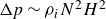
The total horizontal buoyancy force
 $F_b$
can be estimated as the pressure difference in the horizontal
$F_b$
can be estimated as the pressure difference in the horizontal
 $\Delta p$
multiplied by the thickness of the intrusion. The former is the difference in hydrostatic pressure between the intrusion and the ambient, given by
$\Delta p$
multiplied by the thickness of the intrusion. The former is the difference in hydrostatic pressure between the intrusion and the ambient, given by
 $\Delta p \sim \rho _i N^2 H^2$
for the linear ambient density profile and assuming a negligible pressure difference far above the intrusion. Hence
$\Delta p \sim \rho _i N^2 H^2$
for the linear ambient density profile and assuming a negligible pressure difference far above the intrusion. Hence
 \begin{align} F_b \sim H\Delta p \sim \rho _i N^2 H^3. \end{align}
Balancing
 $F_i$
and
$F_i$
and
 $F_b$
, we find the temporal scales
$F_b$
, we find the temporal scales
 \begin{align} H \sim \sqrt {\frac {Q}{N}}, \quad U \sim \sqrt {\textit{NQ}} \quad \text{and} \quad L \sim \sqrt {\textit{NQ}}\,t, \end{align}
indicating that the thickness and speed are constant in time, and the length increases linearly in time.
3. Experiments
3.1. Apparatus and procedures
Quasi-two-dimensional intrusions were generated from a source in a long, thin tank filled with linearly stratified salty water. A flowing ambient was realised by towing the source at constant speed. The experimental set-up is shown in figure 2.
Experimental set-up.
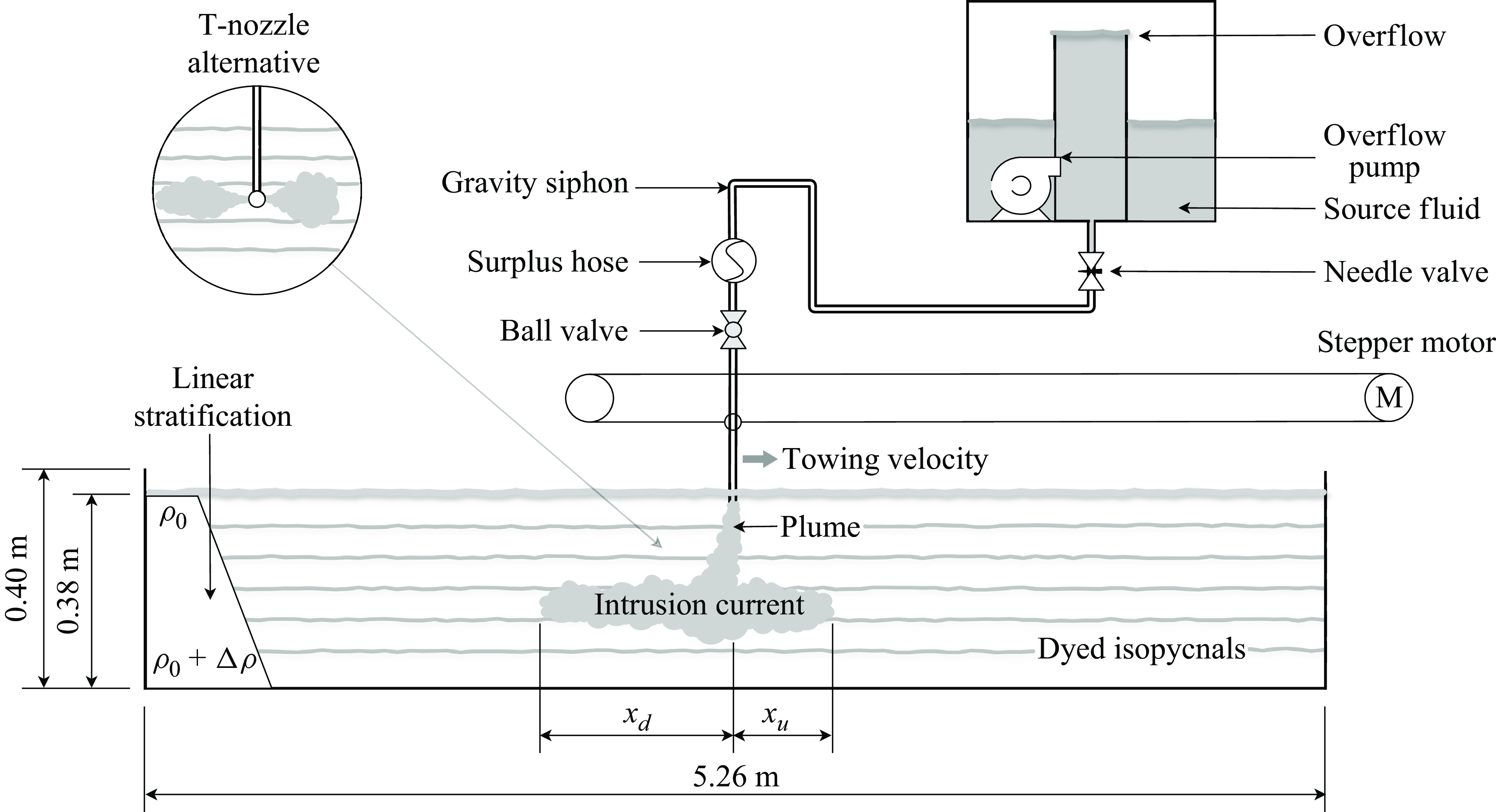
The ambient fluid was set up as follows. A
 $526\ \text{cm}$
long,
$526\ \text{cm}$
long,
 $20\ \text{cm}$
wide tank was filled to depth approximately
$20\ \text{cm}$
wide tank was filled to depth approximately
 $38\ \text{cm}$
with linearly stratified salty water using the double-bucket method (Oster & Yamamoto Reference Oster and Yamamoto1963). At periodic intervals, red food colouring was injected into the supply hose to obtain dyed isopycnal surfaces. The tank was then left for at least two hours to allow diffusion to smear out any density anomalies. The vertical density profile was then obtained by measuring the refractive index at
$38\ \text{cm}$
with linearly stratified salty water using the double-bucket method (Oster & Yamamoto Reference Oster and Yamamoto1963). At periodic intervals, red food colouring was injected into the supply hose to obtain dyed isopycnal surfaces. The tank was then left for at least two hours to allow diffusion to smear out any density anomalies. The vertical density profile was then obtained by measuring the refractive index at
 $5\ \text{cm}$
intervals using an Anton Paar handheld refractometer, and inferring the density using the tables from Lide (Reference Lide2004) with accuracy
$5\ \text{cm}$
intervals using an Anton Paar handheld refractometer, and inferring the density using the tables from Lide (Reference Lide2004) with accuracy
 $0.1\,\%$
. The profile was linear in all experiments, with regression coefficient above
$0.1\,\%$
. The profile was linear in all experiments, with regression coefficient above
 $0.99$
. The density gradient was obtained from a line of best fit, and used to calculate the buoyancy frequency
$0.99$
. The density gradient was obtained from a line of best fit, and used to calculate the buoyancy frequency
 $N = \sqrt {-(g/\rho _b) (\text{d}\rho /\text{d}z)}$
, where
$N = \sqrt {-(g/\rho _b) (\text{d}\rho /\text{d}z)}$
, where
 $\rho _b$
was the density at the base of the tank (taken from the linear fit). In several experiments, crystals of potassium permanganate were dropped into the fluid at various locations along the midline of the tank. As they fell and dissolved, a vertical purple streak was created. This allowed for the visualisation of ambient shear layers during an experiment.
$\rho _b$
was the density at the base of the tank (taken from the linear fit). In several experiments, crystals of potassium permanganate were dropped into the fluid at various locations along the midline of the tank. As they fell and dissolved, a vertical purple streak was created. This allowed for the visualisation of ambient shear layers during an experiment.
Intrusions were generated in this ambient fluid using two different methods: a plume and a diffuser. In both, source fluid was supplied at a constant rate via a gravity feed. A constant pressure head for the feed was ensured by drawing the source fluid from an overflowing cylinder inside a raised bucket. The cylinder was kept in an overflowing state by using a small electric pump to continually add fluid. The source fluid was dyed with blue food colouring to visualise the resulting intrusion.
In the plume method, the source fluid was released into the tank as a negatively buoyant plume with initial density
 $1.11\,\text{g}\ \text{cm}^{-3}$
through a
$1.11\,\text{g}\ \text{cm}^{-3}$
through a
 $10\,\text{mm}$
diameter pipe positioned along the midline of the tank, just below the initial water surface. The source fluid descended, entraining less dense ambient fluid until it reached its level of neutral buoyancy. It then spread horizontally, rapidly extending across the width of the tank. Thereafter, the flow was predominantly along the tank, although the front remained curved in the cross-tank direction. This structure was not analysed in detail. A similar non-uniformity was also observed by Zuluaga-Angel et al. (Reference Zuluaga-Angel, Darden and Fischer1972), who attributed it to secondary flows.
$10\,\text{mm}$
diameter pipe positioned along the midline of the tank, just below the initial water surface. The source fluid descended, entraining less dense ambient fluid until it reached its level of neutral buoyancy. It then spread horizontally, rapidly extending across the width of the tank. Thereafter, the flow was predominantly along the tank, although the front remained curved in the cross-tank direction. This structure was not analysed in detail. A similar non-uniformity was also observed by Zuluaga-Angel et al. (Reference Zuluaga-Angel, Darden and Fischer1972), who attributed it to secondary flows.
In the diffuser method, the source fluid was released at a given depth in the tank. The diffuser consisted of a T-junction connected to a horizontal pipe extending across the width of the tank (see inset to figure 2). The horizontal pipe had
 $144$
holes of
$144$
holes of
 $0.9\pm 0.1\,\text{mm}$
radius on opposite sides (
$0.9\pm 0.1\,\text{mm}$
radius on opposite sides (
 $72$
holes on each side). The source fluid had density equal to the local ambient fluid and was ejected horizontally from the diffuser holes. With this method, the front appeared essentially uniform across the width of the tank.
$72$
holes on each side). The source fluid had density equal to the local ambient fluid and was ejected horizontally from the diffuser holes. With this method, the front appeared essentially uniform across the width of the tank.
In the quiescent ambient experiments, the source was located at the middle of the tank. To replicate a flowing ambient, the source was towed at constant speed using a computer-controlled stepper motor from
 $1/3$
to
$1/3$
to
 $2/3$
of the way across the tank.
$2/3$
of the way across the tank.
Movies of the flows were recorded with three CCD cameras placed approximately
 $4\,\text{m}$
from the tank. The tank was illuminated by three projectors placed approximately
$4\,\text{m}$
from the tank. The tank was illuminated by three projectors placed approximately
 $6\,\text{m}$
away from the tank on the other side, with semi-opaque masks on the camera side of the tank acting as light diffusers. A
$6\,\text{m}$
away from the tank on the other side, with semi-opaque masks on the camera side of the tank acting as light diffusers. A
 $10\ \text{cm}$
grid on the masks aided measurements. Data analysis was primarily of the central camera (a Canon EOS 7D) with
$10\ \text{cm}$
grid on the masks aided measurements. Data analysis was primarily of the central camera (a Canon EOS 7D) with
 $1920\times1080$
pixels giving a spatial resolution of approximately
$1920\times1080$
pixels giving a spatial resolution of approximately
 $1.6\,\text{mm}$
per pixel at
$1.6\,\text{mm}$
per pixel at
 $25$
frames per second. The recordings were processed using MATLAB to extract the shape, area and front positions of the intrusion at each instant. This processing was performed as follows. Each digital image was subtracted from a background image showing the tank prior to the experiment commencing. This image was then split into its red, green and blue colour channels. The red channel was used to analyse the blue intrusion. An appropriate threshold intensity was set for a given experiment to identify the intruding fluid. From this, the overall area of the intrusion, the areas of the upstream and downstream sections, and the front locations
$25$
frames per second. The recordings were processed using MATLAB to extract the shape, area and front positions of the intrusion at each instant. This processing was performed as follows. Each digital image was subtracted from a background image showing the tank prior to the experiment commencing. This image was then split into its red, green and blue colour channels. The red channel was used to analyse the blue intrusion. An appropriate threshold intensity was set for a given experiment to identify the intruding fluid. From this, the overall area of the intrusion, the areas of the upstream and downstream sections, and the front locations
 $x_u$
and
$x_u$
and
 $x_d$
and half-thickness profile
$x_d$
and half-thickness profile
 $h(x,t)$
could be calculated. For the plume experiments, this automatic identification of the intrusion was more difficult, and resulted in an error of approximately
$h(x,t)$
could be calculated. For the plume experiments, this automatic identification of the intrusion was more difficult, and resulted in an error of approximately
 $10\,\%$
in areas. The fronts were particularly difficult to identify automatically, and manual identification was used to find the front velocities accurately. For the diffuser experiments, the colour contrast was stronger; the error in the area was less than
$10\,\%$
in areas. The fronts were particularly difficult to identify automatically, and manual identification was used to find the front velocities accurately. For the diffuser experiments, the colour contrast was stronger; the error in the area was less than
 $5\,\%$
, and the fronts could be automatically identified reliably. Where behaviours appeared to follow a power law in time, the best fit was found using MATLAB’s built-in nonlinear least squares solver, lsqnonlin. In some experiments, further processing of the motion of the isopycnals and streaklines elucidated the behaviour in the ambient.
$5\,\%$
, and the fronts could be automatically identified reliably. Where behaviours appeared to follow a power law in time, the best fit was found using MATLAB’s built-in nonlinear least squares solver, lsqnonlin. In some experiments, further processing of the motion of the isopycnals and streaklines elucidated the behaviour in the ambient.
For the plume experiments, the area of the intrusion increased linearly over time, and the slope of a line of best fit to the area was used to estimate the areal supply rate
 $Q$
. This method was deemed a more direct and accurate way to estimate
$Q$
. This method was deemed a more direct and accurate way to estimate
 $Q$
versus solving the Morton–Taylor–Turner plume equations to infer the mass flux. We could similarly estimate the fluxes to the upstream and downstream portions of the intrusion,
$Q$
versus solving the Morton–Taylor–Turner plume equations to infer the mass flux. We could similarly estimate the fluxes to the upstream and downstream portions of the intrusion,
 $Q_u$
and
$Q_u$
and
 $Q_d$
. For the diffuser experiments, the constant flux
$Q_d$
. For the diffuser experiments, the constant flux
 $Q$
supplied by the source was inferred from a separate experiment. In this, a bucket was placed on a mass balance at an elevation that gave approximately the same pressure head as that driving the flow in the experiments. The weight of water added to the bucket was then recorded over a two-minute interval. Errors in the pressure head were at most 10 %, giving error approximately 5 % in the flux. For both types of source, different fluxes could be achieved by adjusting a needle valve in the supply hose.
$Q$
supplied by the source was inferred from a separate experiment. In this, a bucket was placed on a mass balance at an elevation that gave approximately the same pressure head as that driving the flow in the experiments. The weight of water added to the bucket was then recorded over a two-minute interval. Errors in the pressure head were at most 10 %, giving error approximately 5 % in the flux. For both types of source, different fluxes could be achieved by adjusting a needle valve in the supply hose.
Plume-generated intrusions: experimental values for the ambient properties, source properties and front properties in dimensional and dimensionless form. Ambient properties are the buoyancy frequency
 $N$
and the density at the base of the tank
$N$
and the density at the base of the tank
 $\rho _b$
. Source properties are the source towing speed
$\rho _b$
. Source properties are the source towing speed
 $U_a$
, the height of the intrusion from the base of the tank
$U_a$
, the height of the intrusion from the base of the tank
 $H_i$
, the areal flux to the entire intrusion
$H_i$
, the areal flux to the entire intrusion
 $Q$
, the areal flux to the downstream (left-hand) portion of the intrusion
$Q$
, the areal flux to the downstream (left-hand) portion of the intrusion
 $Q_d$
, the areal flux to the upstream (right-hand) portion of the intrusion
$Q_d$
, the areal flux to the upstream (right-hand) portion of the intrusion
 $Q_u$
, the thickness of the intrusion just downstream of the source
$Q_u$
, the thickness of the intrusion just downstream of the source
 $2h_{\textit{sd}}$
, and the thickness of the intrusion just upstream of the source
$2h_{\textit{sd}}$
, and the thickness of the intrusion just upstream of the source
 $2 h_{su}$
. Front properties are the speed of the downstream front
$2 h_{su}$
. Front properties are the speed of the downstream front
 $u_d$
and upstream front
$u_d$
and upstream front
 $u_u$
in the reference frame of the source. Errors in fluxes and the front velocities are
$u_u$
in the reference frame of the source. Errors in fluxes and the front velocities are
 $10\,\%$
. Errors in heights and thicknesses in this table are the larger of
$10\,\%$
. Errors in heights and thicknesses in this table are the larger of
 $10\,\%$
and
$10\,\%$
and
 $1\,$
cm. Errors in
$1\,$
cm. Errors in
 $U_a$
are less than
$U_a$
are less than
 $2\,\%$
, and those in
$2\,\%$
, and those in
 $N$
are less than
$N$
are less than
 $1\,\%$
. The dimensionless quantities are the dimensionless ambient flow speed
$1\,\%$
. The dimensionless quantities are the dimensionless ambient flow speed
 $U_a/\sqrt{\textit{NQ}}$
, the fraction of supplied fluid that propagates downstream
$U_a/\sqrt{\textit{NQ}}$
, the fraction of supplied fluid that propagates downstream
 $Q_d/Q$
, the Froude number just downstream of the source
$Q_d/Q$
, the Froude number just downstream of the source
 $\mathcal{F}_{\textit{sd}}$
, the Froude number just upstream of the source
$\mathcal{F}_{\textit{sd}}$
, the Froude number just upstream of the source
 $\mathcal{F}_{su}$
, and the dimensionless front speeds. Note that the error in
$\mathcal{F}_{su}$
, and the dimensionless front speeds. Note that the error in
 $\mathcal{F}$
is approximately
$\mathcal{F}$
is approximately
 $30\,\%$
, and up to
$30\,\%$
, and up to
 $50\,\%$
where the values are small.
$50\,\%$
where the values are small.

Finally, Froude numbers (2.3) were estimated for the flows. For the plume experiments, the Froude numbers immediately upstream and downstream of the source were calculated as
 $\mathcal{F}_{\textit{su},\textit{sd}} = Q_{u,d}/(2Nh_{\textit{su},\textit{sd}}^2)$
, where
$\mathcal{F}_{\textit{su},\textit{sd}} = Q_{u,d}/(2Nh_{\textit{su},\textit{sd}}^2)$
, where
 $h_{\textit{su},\textit{sd}}$
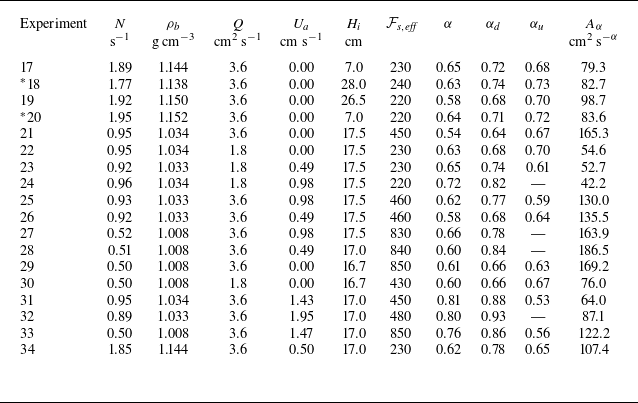
are the half-thicknesses immediately upstream and downstream of the source. For the diffuser experiments, an effective Froude number at the source can be crudely estimated as
$h_{\textit{su},\textit{sd}}$
are the half-thicknesses immediately upstream and downstream of the source. For the diffuser experiments, an effective Froude number at the source can be crudely estimated as
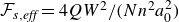 $\mathcal{F}_{s,{\textit{eff}}}=4QW^2/(Nn^2a_0^2)$
, where
$\mathcal{F}_{s,{\textit{eff}}}=4QW^2/(Nn^2a_0^2)$
, where
 $W$
is the width of the tank,
$W$
is the width of the tank,
 $n$
is the number of holes in the diffuser, and
$n$
is the number of holes in the diffuser, and
 $a_0$
is the area of each hole. This estimate comes from the speed at the source being crudely given by
$a_0$
is the area of each hole. This estimate comes from the speed at the source being crudely given by
 $u_0=QW/(n a_0)$
, and the half-thickness at the source being given by
$u_0=QW/(n a_0)$
, and the half-thickness at the source being given by
 $h = Q/(4u_0)$
, with the factor 4 coming from the flux supplying both sides of the intrusion.
$h = Q/(4u_0)$
, with the factor 4 coming from the flux supplying both sides of the intrusion.
The details for the plume experiments are listed in table 1, and those for the diffuser experiments in table 2. For both plume and diffuser, we broadly used two different source strengths. For the diffuser, we used three different stratifications, with
 $N$
approximately
$N$
approximately
 $0.5$
,
$0.5$
,
 $1$
and
$1$
and
 $2\,\text{s}^{-1}$
; for the plume, we used only the two larger values.
$2\,\text{s}^{-1}$
; for the plume, we used only the two larger values.
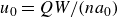
Diffuser-generated intrusions: experimental values for the buoyancy frequency
 $N$
, density at the base of the tank
$N$
, density at the base of the tank
 $\rho _b$
, areal flux
$\rho _b$
, areal flux
 $Q$
, source towing speed
$Q$
, source towing speed
 $U_a$
, height of the intrusion from the base of the tank
$U_a$
, height of the intrusion from the base of the tank
 $H_i$
and effective source Froude number
$H_i$
and effective source Froude number
 $\mathcal{F}_{s,{\textit{eff}}}$
(see text discussion for details). Errors in
$\mathcal{F}_{s,{\textit{eff}}}$
(see text discussion for details). Errors in
 $N$
are
$N$
are
 $1\,\%$
, in
$1\,\%$
, in
 $H_i$
and
$H_i$
and
 $Q$
are less than
$Q$
are less than
 $5\,\%$
, and in
$5\,\%$
, and in
 $U_a$
are less than
$U_a$
are less than
 $2\,\%$
. The additional columns are the best-fit power-law exponents
$2\,\%$
. The additional columns are the best-fit power-law exponents
 $\alpha$
,
$\alpha$
,
 $\alpha _u$
and
$\alpha _u$
and
 $\alpha _d$
for the total area, upstream front location and downstream front location, respectively, as functions of time. The prefactor for the area,
$\alpha _d$
for the total area, upstream front location and downstream front location, respectively, as functions of time. The prefactor for the area,
 $A_\alpha$
, is also given. Where no value is given for the upstream exponent, the fit was poor. In the two experiments marked with
$A_\alpha$
, is also given. Where no value is given for the upstream exponent, the fit was poor. In the two experiments marked with
 $*$
, the experiment was run in the tank left as at the end of the previous experiment.
$*$
, the experiment was run in the tank left as at the end of the previous experiment.
For all experiments, the Reynolds number was above
 $2000$
using (2.4) and using an average rate of change of the area of the intrusion as an estimate for
$2000$
using (2.4) and using an average rate of change of the area of the intrusion as an estimate for
 $Q$
for the diffuser-generated intrusions. However, for intrusions that are nearly arrested by the ambient flow, the value can be significantly lower, and intrusions nearly at the limit of where upstream propagation is possible may have appreciable viscous effects on the upstream side. We further note that viscous effects also increase as the length of the intrusion increases. The time at which viscous and inertial effects are comparable can be estimated as follows. The total viscous forces on the intrusion
$Q$
for the diffuser-generated intrusions. However, for intrusions that are nearly arrested by the ambient flow, the value can be significantly lower, and intrusions nearly at the limit of where upstream propagation is possible may have appreciable viscous effects on the upstream side. We further note that viscous effects also increase as the length of the intrusion increases. The time at which viscous and inertial effects are comparable can be estimated as follows. The total viscous forces on the intrusion
 $F_v$
scale as
$F_v$
scale as
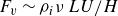 $F_v \sim \rho _i\nu \, L U/H$
, where
$F_v \sim \rho _i\nu \, L U/H$
, where
 $\nu$
is the kinematic viscosity of the flow. Balancing this with
$\nu$
is the kinematic viscosity of the flow. Balancing this with
 $F_i$
in (2.6) gives a time
$F_i$
in (2.6) gives a time
 $Nt \sim Re$
.
$Nt \sim Re$
.
3.2. Plume-generated intrusions
We begin by describing intrusions generated by a negatively buoyant plume, first in a quiescent ambient, and then with relative motion in the ambient. Note that for all experiments, the Froude number on both sides of the source was significantly less than 1 (see table 1), thus the flow in these intrusions was dominated by buoyancy.
3.2.1. Quiescent ambient
In a quiescent ambient, we performed experiments with two different parameter combinations: one case having a weaker source flux in an intermediate stratification (experiment 8 in table 1,
 $N\approx 1\,\text{s}^{-1}$
), and a second case having a stronger source flux in a strong stratification (experiments 15 and 16,
$N\approx 1\,\text{s}^{-1}$
), and a second case having a stronger source flux in a strong stratification (experiments 15 and 16,
 $N\approx 2\,\text{s}^{-1}$
). Figure 3 shows the evolution in the first case; the second case is qualitatively identical, and a final scaled profile is included for comparison in figure 3(g).
$N\approx 2\,\text{s}^{-1}$
). Figure 3 shows the evolution in the first case; the second case is qualitatively identical, and a final scaled profile is included for comparison in figure 3(g).
Initially, a plume descends through the ambient fluid, broadening with depth. It overshoots its level of neutral buoyancy, weakly impacts the base of the tank, then spreads horizontally as an intrusion at approximately
 $1/3$
of the depth of the tank from the bottom. Once the intrusion has spread approximately
$1/3$
of the depth of the tank from the bottom. Once the intrusion has spread approximately
 $10\ \text{cm}$
from the plume, it fills the width of the tank. After this, the downwelling plume appears steady, and the flow within the intrusion appears effectively two-dimensional (although the front remains noticeably curved across the width of the tank for the duration of the experiment). On both sides of the plume, the intrusion now attains a characteristic tapered-wedge profile that elongates in time. Weak turbulence exists in the immediate vicinity of the plume, together with some limited entrainment. Beyond this region, the flow within the intrusion appears laminar, and no further entrainment appears to occur.
$10\ \text{cm}$
from the plume, it fills the width of the tank. After this, the downwelling plume appears steady, and the flow within the intrusion appears effectively two-dimensional (although the front remains noticeably curved across the width of the tank for the duration of the experiment). On both sides of the plume, the intrusion now attains a characteristic tapered-wedge profile that elongates in time. Weak turbulence exists in the immediate vicinity of the plume, together with some limited entrainment. Beyond this region, the flow within the intrusion appears laminar, and no further entrainment appears to occur.
In this regime, the cross-sectional area of the intrusion increases linearly in time (figure 3 d), the fronts propagate at constant velocity (figure 3 e), and the thickness profile of the intrusion has a remarkably good self-similar collapse with the temporal scalings of (2.8) (figure 3 g). The same observations hold for the experiments in the strong case. Furthermore, the front speed scaled by (2.8b ) and the profile thickness scaled by (2.8a ), provide a good collapse of the data between the moderate-case and strong-case experiments (figure 3 g). These observations are thus consistent with the scaling arguments of § 2 for a constantly supplied inertial intrusion.
Plume-generated intrusion in a quiescent ambient (experiment 8 in table 1). (a–c) Snapshots at various times. The white bar in (a) is
 $20\,$
cm long. See movie 1 (supplementary movies are available at https://doi.org/10.1017/jfm.2025.11068). (d) Cross-sectional area and (e) position of the right-hand front as a function of time. The gradients of the dashed lines provide the values of
$20\,$
cm long. See movie 1 (supplementary movies are available at https://doi.org/10.1017/jfm.2025.11068). (d) Cross-sectional area and (e) position of the right-hand front as a function of time. The gradients of the dashed lines provide the values of
 $Q$
and the front velocity
$Q$
and the front velocity
 $u_u$
given in table 1. (f,g) Half-thickness profiles at
$u_u$
given in table 1. (f,g) Half-thickness profiles at
 $5\,\text{s}$
intervals in (f) physical dimensions and (g) rescaled by (2.8). In (d–g), darker curves indicate earlier times, and lighter cyan curves indicate later times. The bold red curves in (g) for
$5\,\text{s}$
intervals in (f) physical dimensions and (g) rescaled by (2.8). In (d–g), darker curves indicate earlier times, and lighter cyan curves indicate later times. The bold red curves in (g) for
 $x\lt 0$
are rescaled, late-time profiles for experiments 15 and 16, with a larger source and stronger stratification.
$x\lt 0$
are rescaled, late-time profiles for experiments 15 and 16, with a larger source and stronger stratification.

3.2.2. Flowing ambient
For a flowing ambient, we performed a series of experiments with varying towing speeds (equivalently varying ambient flow speeds), and
 $N$
and
$N$
and
 $Q$
values corresponding to the first case in a quiescent ambient. We also performed two experiments with a stronger stratification (
$Q$
values corresponding to the first case in a quiescent ambient. We also performed two experiments with a stronger stratification (
 $N\approx 2\,\text{s}^{-1}$
), fixed towing speed (
$N\approx 2\,\text{s}^{-1}$
), fixed towing speed (
 $U_a = 1\ \text{cm}\ \text{s}^{-1}$
), and two different source strengths.
$U_a = 1\ \text{cm}\ \text{s}^{-1}$
), and two different source strengths.

Figure 4 shows the evolution for an intermediate ambient flow speed. The behaviour is similar to that in a quiescent ambient except for asymmetries induced by the ambient flow. The descending plume is slightly bent over in the downstream direction. The intrusion has a thinner, shorter upstream wedge, and a thicker, longer downstream wedge than in the quiescent case. Turbulence in the intrusion is focused immediately downstream of the plume, with some limited concomitant entrainment. In this region, the profile is essentially flat. As for a quiescent ambient, the total cross-sectional area of the intrusion increases linearly in time (figure 4 d), the fronts propagate at constant velocity (figure 4 e), and the thickness profiles of the intrusion (figure 4 f) collapse to a self-similar profile with the scales of (2.8) (figure 4 g).
Key dimensionless quantities for plume-generated intrusions in an ambient flow: (a) downstream and upstream front velocities, rescaled according to (2.8); (b) the fraction of supplied fluid that propagates downstream; (c) the ratio of the upstream and downstream source thicknesses. Solid symbols are for experiments with
 $N\approx 1\,\text{s}^{-1}$
, and open symbols are for experiments with
$N\approx 1\,\text{s}^{-1}$
, and open symbols are for experiments with
 $N\approx 2\,\text{s}^{-1}$
. The grey lines are lines of best fit given by
$N\approx 2\,\text{s}^{-1}$
. The grey lines are lines of best fit given by
 $u_d/\sqrt{\textit{NQ}} = -0.33-0.66U_a/\sqrt{\textit{NQ}}$
for the downstream front velocity,
$u_d/\sqrt{\textit{NQ}} = -0.33-0.66U_a/\sqrt{\textit{NQ}}$
for the downstream front velocity,
 $u_u/\sqrt{\textit{NQ}} = 0.36-1.11U_a/\sqrt{\textit{NQ}}$
for the upstream front velocity, and
$u_u/\sqrt{\textit{NQ}} = 0.36-1.11U_a/\sqrt{\textit{NQ}}$
for the upstream front velocity, and
 $Q_d/Q=0.5 + 1.70U_a/\sqrt{\textit{NQ}}$
for the flux fraction. For the latter fit, the
$Q_d/Q=0.5 + 1.70U_a/\sqrt{\textit{NQ}}$
for the flux fraction. For the latter fit, the
 $0.5$
intercept was enforced.
$0.5$
intercept was enforced.

With increasing ambient flow speeds, the profile asymmetries become increasingly pronounced, the downstream turbulent region expands, and the upstream front speed reduces, but the profile remains self-similar. Figure 5 summarises key features of the intrusions with varying ambient flow speeds. When the ambient flow speed exceeds approximately
 $0.3\sqrt{\textit{NQ}}$
, the intrusion is unable to propagate upstream of the plume (see figure 5
a). For flow speeds close to but below this threshold, the upstream front shows a slight deceleration at late times, and the area of the upstream wedge stops growing. This may be due to viscous effects, but could also be due to difficulties in accurately detecting the intrusion when it was very thin. As the ambient flow speed increases, a significantly larger fraction of the supplied fluid propagates downstream (figure 5
b). The upstream wedge also becomes progressively thinner (figure 5
c).
$0.3\sqrt{\textit{NQ}}$
, the intrusion is unable to propagate upstream of the plume (see figure 5
a). For flow speeds close to but below this threshold, the upstream front shows a slight deceleration at late times, and the area of the upstream wedge stops growing. This may be due to viscous effects, but could also be due to difficulties in accurately detecting the intrusion when it was very thin. As the ambient flow speed increases, a significantly larger fraction of the supplied fluid propagates downstream (figure 5
b). The upstream wedge also becomes progressively thinner (figure 5
c).
3.3. Diffuser-generated intrusions
We now turn to intrusions generated by a diffuser placed at the level of neutral buoyancy of the source fluid. For both quiescent and flowing ambients, we explore the structure across three different stratifications (
 $N\approx 0.5\,\text{s}^{-1}$
,
$N\approx 0.5\,\text{s}^{-1}$
,
 $N\approx 1\,\text{s}^{-1}$
and
$N\approx 1\,\text{s}^{-1}$
and
 $N\approx 2\,\text{s}^{-1}$
) and two different source fluxes (with
$N\approx 2\,\text{s}^{-1}$
) and two different source fluxes (with
 $Q$
differing by a factor of 2). Note that for all of our diffuser experiments, the effective Froude number of the source was of order
$Q$
differing by a factor of 2). Note that for all of our diffuser experiments, the effective Froude number of the source was of order
 $100$
or higher (see table 2), thus the flows are all strongly inertia-dominated at the source.
$100$
or higher (see table 2), thus the flows are all strongly inertia-dominated at the source.
3.3.1. Quiescent ambient
Diffuser-generated intrusions in a quiescent ambient are structurally identical to each other across all of the parameter combinations that we considered. Thus we begin by describing the evolution of one experiment (experiment 22), shown in figure 6, in detail.
Diffuser-generated intrusion in a quiescent ambient (experiment 22 in table 2). (a–c) Snapshots at various times. The white bar in (a) is
 $20\,$
cm long. See supplementary movie 3. (d) Cross-sectional area and (e) position of the fronts, respectively, as functions of time since initiation of the source. The power-law fits shown by the accompanying dashed curves are given in table 2. In (d), the solid black line is the area increase based on the source flux alone. (f,g) Half-thickness profiles at
$20\,$
cm long. See supplementary movie 3. (d) Cross-sectional area and (e) position of the fronts, respectively, as functions of time since initiation of the source. The power-law fits shown by the accompanying dashed curves are given in table 2. In (d), the solid black line is the area increase based on the source flux alone. (f,g) Half-thickness profiles at
 $5\,\text{s}$
intervals: (f) in physical dimensions, and (g) with
$5\,\text{s}$
intervals: (f) in physical dimensions, and (g) with
 $x$
rescaled by the front position
$x$
rescaled by the front position
 $x_u(t)$
. In (d–g), darker curves indicate earlier times, and lighter curves indicate later times.
$x_u(t)$
. In (d–g), darker curves indicate earlier times, and lighter curves indicate later times.

The intrusion structure is significantly different from the plume-generated case. Immediately next to the diffuser, the intrusion thickens substantially to a maximum a few centimetres away. This can be interpreted as an entraining hydraulic jump following Zuluaga-Angel et al. (Reference Zuluaga-Angel, Darden and Fischer1972), or alternatively as an expanding jet. In either case, the flow transitions from a jet-like flow at the diffuser to a buoyancy-dominated flow further away: at the diffuser, the Froude number is significantly above
 $100$
, as noted above, while ahead of this region, it is of order
$100$
, as noted above, while ahead of this region, it is of order
 $0.1$
based on the thickness of the flow and the speed of the front.
$0.1$
based on the thickness of the flow and the speed of the front.
Beyond> this, the intrusion gradually thins in a region that lengthens over time and then thins more rapidly to the front. The profiles in the near-source region, and plausibly the gradually thinning region, appear steady. A steady near-source region is expected for a constant, supercritical source. The rapidly thinning frontal region is plausibly self-similar on rescaling the horizontal coordinate
 $x$
by the frontal position
$x$
by the frontal position
 $x_u(t)$
(figure 6
g).
$x_u(t)$
(figure 6
g).
Entrainment into the intrusion is appreciable, with its area significantly larger than what would be predicted based on the constant supply rate
 $Q$
alone (curve versus black line in figure 6
d). This entrainment appears to occur via billows along the top and bottom interfaces of the intrusion in the near-source region. The overall rate of entrainment reduces over time, with the area of the intrusion increasing sublinearly as
$Q$
alone (curve versus black line in figure 6
d). This entrainment appears to occur via billows along the top and bottom interfaces of the intrusion in the near-source region. The overall rate of entrainment reduces over time, with the area of the intrusion increasing sublinearly as
 $t^{0.63}$
(figure 6
d).
$t^{0.63}$
(figure 6
d).
The fronts also propagate as decelerating power laws in time, with the two front positions proportional to
 $t^{0.68}$
and
$t^{0.68}$
and
 $t^{0.70}$
, respectively. We note that these power laws are reasonably consistent with the temporal behaviour observed for the area and the observed steady thickness. Unsurprisingly, as the area is not increasing linearly, this behaviour is not consistent with the temporal scales of (2.8). Allowing for a variable source flux to match the observed areal behaviour predicts fronts that propagate as
$t^{0.70}$
, respectively. We note that these power laws are reasonably consistent with the temporal behaviour observed for the area and the observed steady thickness. Unsurprisingly, as the area is not increasing linearly, this behaviour is not consistent with the temporal scales of (2.8). Allowing for a variable source flux to match the observed areal behaviour predicts fronts that propagate as
 $t^{0.82}$
and a thickness that decreases as
$t^{0.82}$
and a thickness that decreases as
 $t^{-0.18}$
(see Appendix A for details). The difference in the frontal power-law exponent may be due to the fit not accounting for the initial adjustment period while the hydraulic jump forms. However, the decrease in the thickness over time is incompatible with the steady near-source behaviour observed. This suggests that the simple inertia–buoyancy balance of § 2 may not be sufficient to describe these flows.
$t^{-0.18}$
(see Appendix A for details). The difference in the frontal power-law exponent may be due to the fit not accounting for the initial adjustment period while the hydraulic jump forms. However, the decrease in the thickness over time is incompatible with the steady near-source behaviour observed. This suggests that the simple inertia–buoyancy balance of § 2 may not be sufficient to describe these flows.
Downstream (a,b) front positions and (c,d) intrusion profiles for all diffuser-generated intrusions in a quiescent ambient. In (c) and (d), the profiles are for times
 $t=40/N$
. Plots in (a) and (c) are dimensional; those in (b) and (d) are rescaled according to (2.2). Colours and experiment numbers: blue for 17, red for 18, yellow for 19, purple for 20, green for 21, cyan for 22, deep red for 29, and black for 30.
$t=40/N$
. Plots in (a) and (c) are dimensional; those in (b) and (d) are rescaled according to (2.2). Colours and experiment numbers: blue for 17, red for 18, yellow for 19, purple for 20, green for 21, cyan for 22, deep red for 29, and black for 30.

Looking across all experiments in a quiescent ambient, the non-dimensionalisation based on
 $Q$
and
$Q$
and
 $N$
given by (2.2) gives a good collapse of the data (see figure 7). Across the experiments, the power-law exponents are also similar (see the
$N$
given by (2.2) gives a good collapse of the data (see figure 7). Across the experiments, the power-law exponents are also similar (see the
 $\alpha$
parameters in table 2).
$\alpha$
parameters in table 2).
3.3.2. Flowing ambient
Turning to a flowing ambient, figure 8 shows the evolution of a diffuser-generated intrusion for a strong source, in a weakly stratified ambient with a moderate ambient flow.

Because of the combination of increased source strength and decreased buoyancy frequency, this flow is significantly thicker than that shown in figure 6. Structurally, the evolution is similar to that for a quiescent fluid with a steady near-source hydraulic jump connecting to a steady thinning region and a propagating tip region in which the intrusion thins to the front. However, there is a notable asymmetry between the two sides. On the upstream side, the slope of the steady thinning region is the same as for the tip region, and the intrusion appears to develop into a steady linear wedge. On the downstream side, the steady region appears to take longer to establish than in the quiescent case. Notably, the maximum thickness is the same on both sides.
The total area of the intrusion increases similarly to the quiescent case, as
 $t^{0.66}$
. However, the location of the upstream front cannot be described particularly well by a power law, and the downstream front propagates with a larger exponent, as
$t^{0.66}$
. However, the location of the upstream front cannot be described particularly well by a power law, and the downstream front propagates with a larger exponent, as
 $t^{0.78}$
.
$t^{0.78}$
.
(a) Front positions against time, and (b–d) selected thickness profiles for all diffuser-generated intrusions in a flowing ambient, together with experiment 17 in a quiescent ambient. Quantities are rescaled according to (2.2). The profiles in (b–d) are at the times indicated. The colour throughout indicates the value of the dimensionless ambient flow speed
 $U_a/\sqrt{\textit{NQ}}$
, with darker colours indicating smaller values, and lighter colours indicating larger values.
$U_a/\sqrt{\textit{NQ}}$
, with darker colours indicating smaller values, and lighter colours indicating larger values.

Looking across all experiments and non-dimensionalising using (2.2), we obtain the front location and profile plots of figure 9. Experiments with the same
 $U_a/\sqrt{\textit{NQ}}$
collapse using this scaling. Across different
$U_a/\sqrt{\textit{NQ}}$
collapse using this scaling. Across different
 $U_a/\sqrt{\textit{NQ}}$
, the upstream/downstream asymmetry increases, although the maximum thickness does not appear to change significantly. For
$U_a/\sqrt{\textit{NQ}}$
, the upstream/downstream asymmetry increases, although the maximum thickness does not appear to change significantly. For
 $U_a/\sqrt{\textit{NQ}}\gtrsim 0.6$
, the upstream front appears effectively stationary in the frame of reference of the source by the end of the experiment (see figure 9
a). If the experiments ran for longer in a larger tank, then we anticipate that the upstream front in all experiments would become stationary because eventually the decelerating tip speed can no longer exceed the ambient flow speed. We note that the power-law exponent for the downstream front increases with increasing ambient flow speed (see table 2).
$U_a/\sqrt{\textit{NQ}}\gtrsim 0.6$
, the upstream front appears effectively stationary in the frame of reference of the source by the end of the experiment (see figure 9
a). If the experiments ran for longer in a larger tank, then we anticipate that the upstream front in all experiments would become stationary because eventually the decelerating tip speed can no longer exceed the ambient flow speed. We note that the power-law exponent for the downstream front increases with increasing ambient flow speed (see table 2).
3.4. Dynamics in the ambient fluid
Finally, we briefly consider the dynamics in the ambient fluid, and how this can feed back on the intrusion. Figure 10 shows various observations in the ambient fluid for experiment 8, the exemplar experiment for plume-generated intrusions in a quiescent ambient. These observations are: the motion of an initially vertical potassium permanganate streak over time (figure 10 a), the evolution of a given vertical slice over time (figure 10 b), and the vertical displacement over time of an isopycnal immediately below the intrusion (figure 10 c) and immediately above it (figure 10 d).
Dynamics in the ambient fluid for experiment 8. (a) Time evolution of the potassium permanganate streak closest to the intrusion. Curves are at
 $5\,$
s intervals, with darker colours indicating earlier times, and lighter colours indicating later times. The colour-to-time conversion is the same as in figure 3. (b) Time evolution of a vertical slice
$5\,$
s intervals, with darker colours indicating earlier times, and lighter colours indicating later times. The colour-to-time conversion is the same as in figure 3. (b) Time evolution of a vertical slice
 $80\,$
cm from the source. (c,d) Vertical displacements of the isopycnals (c) immediately below and (d) immediately above the intrusion over time. The white lines in (c,d) show the locations of the slice in (b), and the red lines show the locations of the fronts. The selected streak, slice and isopycnals are also indicated by arrows on the right-hand side of figure 3
a.
$80\,$
cm from the source. (c,d) Vertical displacements of the isopycnals (c) immediately below and (d) immediately above the intrusion over time. The white lines in (c,d) show the locations of the slice in (b), and the red lines show the locations of the fronts. The selected streak, slice and isopycnals are also indicated by arrows on the right-hand side of figure 3
a.

The dominant motion is an exchange flow, with a prominent flow away from the source at the height of the intrusion, a return flow towards the source in the top half of the tank, and at later times a second, narrower return flow at the bottom boundary. This motion is clearly evident in the evolution of the potassium permanganate streak (figure 10
a). This exchange flow results in the isopycnal beneath the intrusion being depressed by a near-uniform
 $0.7\,$
cm in a growing region around the intrusion, and the isopycnal above it being raised by a near-uniform
$0.7\,$
cm in a growing region around the intrusion, and the isopycnal above it being raised by a near-uniform
 $1.5\,$
cm. This is apparent in the slice image (figure 10
b) where a noticeable displacement of the first and third red isopycnals begins at approximately
$1.5\,$
cm. This is apparent in the slice image (figure 10
b) where a noticeable displacement of the first and third red isopycnals begins at approximately
 $t=20$
–
$t=20$
–
 $30\,$
s, and also in the isopycnal displacement panels at the sharp yellow–green transition extending linearly from the origin in figure 10(c), and the sharp blue–green transition in figure 10(d). The region of isopycnal displacement appears to grow at approximately twice the speed of the intrusion tip (thus it reaches the end walls of the tank after approximately
$30\,$
s, and also in the isopycnal displacement panels at the sharp yellow–green transition extending linearly from the origin in figure 10(c), and the sharp blue–green transition in figure 10(d). The region of isopycnal displacement appears to grow at approximately twice the speed of the intrusion tip (thus it reaches the end walls of the tank after approximately
 $80$
–
$80$
–
 $100\,$
s). Note that this displacement of the isopycnals results in a decrease in the local density gradient and hence a decrease in the buoyancy frequency ahead of the intrusion. The factor for the former can be calculated as the ratio of the initial gap between the isopycnals to the final gap,
$100\,$
s). Note that this displacement of the isopycnals results in a decrease in the local density gradient and hence a decrease in the buoyancy frequency ahead of the intrusion. The factor for the former can be calculated as the ratio of the initial gap between the isopycnals to the final gap,
 $10\ \text{cm}/12.2\ \text{cm} \approx 0.82$
. This gives a corresponding decrease in the buoyancy frequency
$10\ \text{cm}/12.2\ \text{cm} \approx 0.82$
. This gives a corresponding decrease in the buoyancy frequency
 $N$
by a factor of approximately
$N$
by a factor of approximately
 $0.91$
.
$0.91$
.
We interpret this exchange flow as the result of entrainment of ambient fluid into the plume supplying the intrusion. Crudely estimating the volume increase in the plume using a Morton–Taylor–Turner description suggests that
 $90\,\%$
of the supply to the intrusion originates from entrainment of ambient fluid (see also Hogg et al. Reference Hogg, Hallworth and Huppert2005). This means that a return flow must exist in the ambient that is almost as strong as the flow driven by the intrusion itself.
$90\,\%$
of the supply to the intrusion originates from entrainment of ambient fluid (see also Hogg et al. Reference Hogg, Hallworth and Huppert2005). This means that a return flow must exist in the ambient that is almost as strong as the flow driven by the intrusion itself.
Superimposed on this exchange flow are smaller-amplitude internal gravity waves. The fastest such waves are visible as a
 $\Delta y \approx 0.2\ \text{cm}$
brighter yellow region extending linearly from the origin at early times in figure 10(c) (reaching
$\Delta y \approx 0.2\ \text{cm}$
brighter yellow region extending linearly from the origin at early times in figure 10(c) (reaching
 $x=150\ \text{cm}$
at
$x=150\ \text{cm}$
at
 $t\approx 20\,\text{s}$
), and equivalent light blue regions at early times in figure 10(d). These waves have amplitude only
$t\approx 20\,\text{s}$
), and equivalent light blue regions at early times in figure 10(d). These waves have amplitude only
 $1$
–
$1$
–
 $2\,$
mm (approximately a single pixel) and speed
$2\,$
mm (approximately a single pixel) and speed
 $6$
–
$6$
–
 $7\,$
cm s−1. They could plausibly be mode-2 long waves (see e.g. Turner Reference Turner1973), whose speed in the tank is
$7\,$
cm s−1. They could plausibly be mode-2 long waves (see e.g. Turner Reference Turner1973), whose speed in the tank is
 $5.6\,$
cm s−1. Within the region of influence of the exchange flow, internal waves are also present. These waves are slower near the source, where they propagate at
$5.6\,$
cm s−1. Within the region of influence of the exchange flow, internal waves are also present. These waves are slower near the source, where they propagate at
 $2$
–
$2$
–
 $3\,$
cm s−1, and faster further from the source, where they propagate at
$3\,$
cm s−1, and faster further from the source, where they propagate at
 $4$
–
$4$
–
 $5\,$
cm s−1. They have wavelength
$5\,$
cm s−1. They have wavelength
 $20$
–
$20$
–
 $30\,$
cm. The speed of these waves does not match with the speed of any linear modes of this wavelength: mode-1 waves are predicted to have speed
$30\,$
cm. The speed of these waves does not match with the speed of any linear modes of this wavelength: mode-1 waves are predicted to have speed
 $2.8$
–
$2.8$
–
 $4.1\,$
cm s−1, mode-2 waves
$4.1\,$
cm s−1, mode-2 waves
 $2.6$
–
$2.6$
–
 $3.4\,$
cm s−1, and mode-3 waves
$3.4\,$
cm s−1, and mode-3 waves
 $2.3$
–
$2.3$
–
 $2.8\,$
cm s−1. However, these waves are likely influenced by the exchange flow, while the predictions are for a quiescent ambient and so are not directly applicable.
$2.8\,$
cm s−1. However, these waves are likely influenced by the exchange flow, while the predictions are for a quiescent ambient and so are not directly applicable.
In this experiment, and others with a moderate or strong stratification, the internal waves appear to provide minimal feedback on the intrusion. However, for weakly stratified ambients, there is a clear feedback. An example is shown in figure 8. Focusing on the upstream (right-hand) front, a thickened bolus forms at the front associated with the crest of a wave (figure 8 a). This wave propagates faster than the front, so the trough of the wave begins to the squeeze the bolus from behind (figure 8 b) to form a thin, flattened tip (figure 8 c). This cycle then repeats as the crest of the next wave approaches the front. The same behaviour also occurs at the downstream (left-hand) front, and is particularly evident in the half-thickness profiles (figure 8 f). This interaction results in a pulsing overtone to the propagation of the fronts. Similar behaviour is also observed in experiments 22, 29 and 30 (see figure 7). However, despite this clear signature of the waves on the intrusion profiles and propagation, they do not appear to cause a fundamental change in the intrusion behaviour, and the data from these experiments collapse with data from experiments having no appreciable feedback (see figures 7 and 9).
Finally, we performed four experiments to explore the impact of perturbations to the ambient density profile away from the intrusion by running two experiments in succession at different heights in the tank without refilling (experiments 17–20). No perceptible qualitative or quantitative differences were observed, suggesting that only the local stratification is important, although the resulting density perturbations were quite small.
4. Intrusive shallow-water modelling
We now turn to theoretical modelling using the intrusive shallow-water model of Ungarish (Reference Ungarish2005) with the addition of a line source and an ambient flow. The configuration and relevant variables are shown in figure 1. Our aim is to assess the validity of this model against experimental data in a geometry in which it has not previously been tested. In using it, we are requiring that the intrusions are slender and with motion controlled by a balance between inertia and buoyancy. Significantly, the model does not incorporate entrainment, thus the results are only directly applicable to the plume-generated intrusion experiments.
4.1. Formulation
The governing equations for conservation of mass and momentum are
 \begin{align} \frac {\partial h}{\partial t} + \frac {\partial }{\partial x}(\bar {u} h) &= \frac {1}{2}q(x) \end{align}
and
 \begin{align} \frac {\partial }{\partial t}(\bar {u} h) + \frac {\partial }{\partial x}\left (\bar {u}^2h + \frac {1}{3}N^2 h^3\right ) &= \frac {1}{2}q_{\textit{mom}}(x), \end{align}
respectively. Here,
 $h(x,t)$
is the half-thickness of the intrusion,
$h(x,t)$
is the half-thickness of the intrusion,
 $\bar {u}(x,t)$
is the vertically averaged horizontal velocity of the intrusion,
$\bar {u}(x,t)$
is the vertically averaged horizontal velocity of the intrusion,
 $q(x)$
is the volume-flux distribution of the source, and
$q(x)$
is the volume-flux distribution of the source, and
 $q_{\textit{mom}}(x)$
the specific momentum-flux distribution of the source. The factors of
$q_{\textit{mom}}(x)$
the specific momentum-flux distribution of the source. The factors of
 $1/2$
result from these fluxes supplying both the top and bottom halves of the intrusion.
$1/2$
result from these fluxes supplying both the top and bottom halves of the intrusion.
The source distribution functions
 $q(x)$
and
$q(x)$
and
 $q_{\textit{mom}}(x)$
are not known in detail for the experiments, and cannot readily be modelled rigorously. Fortunately, complete details are not required for the plume-generated intrusions. For these experiments,
$q_{\textit{mom}}(x)$
are not known in detail for the experiments, and cannot readily be modelled rigorously. Fortunately, complete details are not required for the plume-generated intrusions. For these experiments,
 $\mathcal{F}_s\leqslant 1$
on both sides of the source region, and the theory of hyperbolic partial differential equations dictates that only two pieces of information can be incorporated from the source (Kevorkian Reference Kevorkian1990). These are the overall areal supply rate and net momentum supply rate to the intrusion, i.e.
$\mathcal{F}_s\leqslant 1$
on both sides of the source region, and the theory of hyperbolic partial differential equations dictates that only two pieces of information can be incorporated from the source (Kevorkian Reference Kevorkian1990). These are the overall areal supply rate and net momentum supply rate to the intrusion, i.e.
 \begin{align} \left [\bar {u} h\right ] = \frac {1}{2}Q = \frac {1}{2}\int q(x) \quad \text{and} \quad \left [\bar {u}^2h + \frac {1}{3}N^2 h^3\right ] = \frac {1}{2}Q_{\textit{mom}} = \frac {1}{2}\int q_{\textit{mom}}(x), \end{align}
respectively, where
 $[{\cdot }]$
is the difference in the bracketed quantity across the source, and the integral is across the source region. Note that this form of the source conditions does not prescribe the fraction of fluid that propagates upstream and downstream; this will be determined as part of the solution.
$[{\cdot }]$
is the difference in the bracketed quantity across the source, and the integral is across the source region. Note that this form of the source conditions does not prescribe the fraction of fluid that propagates upstream and downstream; this will be determined as part of the solution.
We further note that the source Froude numbers are not known a priori, but are also part of the solution. We therefore test that the Froude number restrictions are met in the solutions that we present. In Appendix B, we find solutions for an illustrative source distribution without these Froude number restrictions to give an indication of when the source details matter and to provide further explanation of some of the steps below. Finally, we note that in general, shocks may develop in the hyperbolic equations (4.1). However, with the Froude number restriction at the source, such solutions are not possible. We also discuss this further in Appendix B.
4.1.1. Boundary conditions
Form drag from the ambient is captured using a fixed Froude number condition at the front. We impose this condition in the reference frame of the ambient flow to incorporate the latter’s effect. A kinematic boundary condition captures conservation of mass. Thus at the downstream front at
 $x=x_d(t)$
,
$x=x_d(t)$
,
 \begin{align} \frac {\text{d} x_d}{\text{d}{t}} = u_d \quad \text{and} \quad u_d + U_a = -\beta N h_d, \end{align}
and at the upstream front at
 $x=x_u(t)$
,
$x=x_u(t)$
,
 \begin{align} \frac {\text{d} x_u}{\text{d}{t}} = u_u \quad \text{and} \quad u_u + U_a = \beta N h_u, \end{align}
where
 $\beta$
is the value of the imposed Froude number. In the model of Ungarish (Reference Ungarish2005),
$\beta$
is the value of the imposed Froude number. In the model of Ungarish (Reference Ungarish2005),
 $\beta$
is related to the frontal Froude number for gravity currents
$\beta$
is related to the frontal Froude number for gravity currents
 $\beta _{{gc}}$
through
$\beta _{{gc}}$
through
 $\beta =\beta _{{gc}}/\sqrt {2}$
. For the inviscid limit where
$\beta =\beta _{{gc}}/\sqrt {2}$
. For the inviscid limit where
 $\beta _{{gc}}=\sqrt {2}$
(Benjamin Reference Benjamin1968), we then have
$\beta _{{gc}}=\sqrt {2}$
(Benjamin Reference Benjamin1968), we then have
 $\beta =1$
. In real systems, viscous, turbulent and wave drag are thought to reduce
$\beta =1$
. In real systems, viscous, turbulent and wave drag are thought to reduce
 $\beta$
, and Ungarish (Reference Ungarish2005) bases the value on the empirical gravity–current relationship of Huppert & Simpson (Reference Huppert and Simpson1980). For a deep ambient, this yields
$\beta$
, and Ungarish (Reference Ungarish2005) bases the value on the empirical gravity–current relationship of Huppert & Simpson (Reference Huppert and Simpson1980). For a deep ambient, this yields
 $\beta =0.84$
. For an intrusion filling approximately a third of the depth of the tank, as was typically the case for our plume-generated intrusions,
$\beta =0.84$
. For an intrusion filling approximately a third of the depth of the tank, as was typically the case for our plume-generated intrusions,
 $\beta \approx 0.5$
.
$\beta \approx 0.5$
.
4.2. Similarity solutions
We look for similarity solutions to match the observed experimental forms. At sufficiently long times, the intrusions extend far beyond the source region, and the source width is no longer relevant. The remaining important parameters are
 $NQ$
,
$NQ$
,
 $NQ_{\textit{mom}}$
and
$NQ_{\textit{mom}}$
and
 $U_a$
, all of whose dimensions are powers of
$U_a$
, all of whose dimensions are powers of
 ${\textrm{L}}/{\textrm{T}}$
. Because only a single dimensional grouping remains, there is no length scale for the problem, and we expect similarity solutions to exist (Barenblatt Reference Barenblatt1996).
${\textrm{L}}/{\textrm{T}}$
. Because only a single dimensional grouping remains, there is no length scale for the problem, and we expect similarity solutions to exist (Barenblatt Reference Barenblatt1996).
We set the similarity variable to be
 \begin{align} \eta = x/\sqrt{\textit{NQ}}\, t, \end{align}
and the velocity and buoyancy profiles to be
 \begin{align} \bar {u} = \sqrt{\textit{NQ}}\,\mathcal{U}(\eta ) \quad \text{and} \quad Nh = \sqrt{\textit{NQ}}\,\mathcal{H}(\eta ), \end{align}
respectively, where
 $\mathcal{U}(\eta )$
and
$\mathcal{U}(\eta )$
and
 $\mathcal{H}(\eta )$
are unknown functions to be found. Substituting these forms into (4.1), we obtain the system of ordinary differential equations
$\mathcal{H}(\eta )$
are unknown functions to be found. Substituting these forms into (4.1), we obtain the system of ordinary differential equations
 \begin{align} -\eta \,\mathcal{H}' + (\mathcal{U}\mathcal{H})' = 0 \quad \text{and} \quad {-\eta} \,\mathcal{U}' + \mathcal{U}\mathcal{U}' + \mathcal{H}\mathcal{H}' = 0 \end{align}
outside the source region, with primes indicating derivatives. Solutions to this system are
 $\mathcal{U}$
and
$\mathcal{U}$
and
 $\mathcal{H}$
constant, and the wedge-like rarefaction solution
$\mathcal{H}$
constant, and the wedge-like rarefaction solution
 \begin{align} \mathcal{U} = \mathcal{U}_0 + \eta /2, \quad \mathcal{H} = |\mathcal{U}-\eta | = |\mathcal{U}_0 - \eta /2|, \end{align}
where
 $\mathcal{U}_0$
is a constant.
$\mathcal{U}_0$
is a constant.
To create a complete solution, these two solution forms must be combined appropriately to satisfy the conditions across the source and the frontal boundary conditions. With the condition that the source Froude number is less than or equal to 1, the possible combined forms on one side of the source are
-
(i) a single constant state satisfying the frontal boundary conditions (denoted a type C solution) given by
(4.9)where \begin{align} \mathcal{U} = \mathcal{U}_f, \quad \mathcal{H} = \mathcal{H}_f \quad \text{for } |\eta |\lt |\eta _f|, \end{align}
$\mathcal{U}_f$
and
$\mathcal{H}_f$
are constants, and
$\eta _f$
is the location of the front in similarity form,
\begin{align} \mathcal{U} = \mathcal{U}_f, \quad \mathcal{H} = \mathcal{H}_f \quad \text{for } |\eta |\lt |\eta _f|, \end{align}
$\mathcal{U}_f$
and
$\mathcal{H}_f$
are constants, and
$\eta _f$
is the location of the front in similarity form,
-
(ii) a rarefaction at the source connecting continuously to a constant state satisfying the frontal boundary conditions (denoted a type RC solution) given by
(4.10)where
\begin{align} \mathcal{U} = \begin{cases} \mathcal{U}_0 + \eta /2, & |\eta |\lt |\eta _j|,\\ \mathcal{U}_0 + \eta _j/2, & |\eta _j|\lt |\eta |\lt |\eta _f|, \end{cases} \quad \text{and} \quad \mathcal{H} = \begin{cases} |\mathcal{U}_0 - \eta /2|, & |\eta |\lt |\eta _j|,\\ |\mathcal{U}_0 - \eta _j/2|, & |\eta _j|\lt |\eta |\lt |\eta _f|, \end{cases} \end{align}
$\eta _j$
is the location of the graft between the rarefaction near the source and the constant solution at the front.


In similarity form, the conditions across the source (4.2) become
 \begin{align} \left [\mathcal{U}\mathcal{H}\right ] = \frac {1}{2} \quad \text{and} \quad \left [\mathcal{U}^2\mathcal{H} + \frac {1}{3}\mathcal{H}^3\right ] = \frac {1}{2}\frac {NQ_{\textit{mom}} }{(NQ)^{3/2}}, \end{align}
and the frontal boundary conditions become
 \begin{align} \eta _{d} = \mathcal{U}_d \quad \text{and} \quad \mathcal{U}_d+\mathcal{U}_a = -\beta \mathcal{H}_d \end{align}
at the downstream front, and
 \begin{align} \eta _{u} = \mathcal{U}_u \quad \text{and} \quad \mathcal{U}_u+\mathcal{U}_a = \beta \mathcal{H}_u \end{align}
at the upstream front, where
 $\,\mathcal{U}_a = \displaystyle {U_a/\sqrt{\textit{NQ}}}$
.
$\,\mathcal{U}_a = \displaystyle {U_a/\sqrt{\textit{NQ}}}$
.
The appropriate set of algebraic equations arising from (4.9)–(4.12) can be solved using MATLAB’s fsolve numerical solver. (It can be shown that there is either a unique solution or no solution for given parameter values; see Appendix B.)
We now explore the structure of these solutions across parameter space. Throughout, we use the notation X-Y to denote that the solution is type X upstream of the source, and type Y downstream of the source.
4.2.1. Quiescent ambients
We begin with intrusions in a quiescent ambient,
 $U_a=0$
, without a net source of momentum,
$U_a=0$
, without a net source of momentum,
 $Q_{\textit{mom}}=0$
. In this scenario, the intrusions are left/right symmetric and are type C-C for the relevant range of
$Q_{\textit{mom}}=0$
. In this scenario, the intrusions are left/right symmetric and are type C-C for the relevant range of
 $\beta$
values,
$\beta$
values,
 $\beta \leqslant 1$
. The solutions can be found analytically as
$\beta \leqslant 1$
. The solutions can be found analytically as
 \begin{align} \mathcal{H} = 1/\big(2\sqrt {\beta }\big) \quad \text{and} \quad \mathcal{U} = \operatorname {sign}(\eta )\sqrt {\beta }/2. \end{align}
We note that these solutions correspond exactly to box-model predictions (Ungarish Reference Ungarish2020), although their rectangular shape is an outcome of the equations rather than an assumption.
Similarity solutions of the intrusive shallow-water model for a constant source and a flowing ambient: type of solution as a function of ambient flow speed
 $\mathcal{U}_a$
and (a) frontal Froude number
$\mathcal{U}_a$
and (a) frontal Froude number
 $\beta$
with
$\beta$
with
 $Q_{\textit{mom}}=0$
, or (b) net momentum
$Q_{\textit{mom}}=0$
, or (b) net momentum
 $Q_{\textit{mom}}$
with
$Q_{\textit{mom}}$
with
 $\beta =0.4$
. In both plots, the bold curve indicates
$\beta =0.4$
. In both plots, the bold curve indicates
 $u_u=0$
, beyond which no upstream propagation occurs. In (b), the bold dashed curve corresponds to zero downstream thickness. (c,d) Half-thickness and velocity profiles, respectively, for
$u_u=0$
, beyond which no upstream propagation occurs. In (b), the bold dashed curve corresponds to zero downstream thickness. (c,d) Half-thickness and velocity profiles, respectively, for
 $\beta =0.8$
and
$\beta =0.8$
and
 $\mathcal{U}_a$
from
$\mathcal{U}_a$
from
 $0$
to
$0$
to
 $0.8$
in steps of
$0.8$
in steps of
 $0.2$
. The thin grey curve in (b) gives the relationship
$0.2$
. The thin grey curve in (b) gives the relationship
 $Q_{\textit{mom}}=-0.9\mathcal{U}_a$
.
$Q_{\textit{mom}}=-0.9\mathcal{U}_a$
.

Comparison between solutions of the shallow-water equations (in black) and experimental data (in grey) for plume-generated intrusions. (a,b) Half-thickness profiles corresponding to (a) the quiescent ambient case shown in figure 3(g), and (b) the flowing ambient case shown in figure 4(g) (experiments 8 and 7, respectively). (c) The predicted front velocities, (d) the fraction of fluid propagating downstream, and (e) the ratio of the upstream to downstream source heights as functions of ambient flow speed. Experimental data are from figure 5. In (c–e), the solid black curve has no net momentum,
 $Q_{\textit{mom}} =0$
, and the dashed curve has
$Q_{\textit{mom}} =0$
, and the dashed curve has
 $Q_{\textit{mom}} = -0.9U_a$
.
$Q_{\textit{mom}} = -0.9U_a$
.

4.2.2. Flowing ambients
For flowing ambients, the possible types of solution across parameter space are shown in figure 11. The solutions are now asymmetric, with a shorter, thicker upstream section, and a longer, thinner downstream section (see figure 11 c). This reflects the increased ambient resistance and more restricted propagation when the intrusion is counter-flowing, and decreased resistance and easier propagation when the intrusion is co-flowing.
Significantly, there> are now regions of parameter space where no solution exists. In some regions, this results from the ambient flow being so strong that no material flows upstream (bold curves in figures 11 a,b), or from the ease with which material flows downstream resulting in zero downstream frontal thickness (dashed curve in figure 11 b).
Intrusions of type C-RC dominate for intrusions with non-negligible ambient flow. The maximum ambient flow speed
 $\mathcal{U}_{a,max }$
for which such intrusions propagate upstream can be found analytically. At this limiting value, the type C upstream solution is
$\mathcal{U}_{a,max }$
for which such intrusions propagate upstream can be found analytically. At this limiting value, the type C upstream solution is
 $\mathcal{U} = 0$
,
$\mathcal{U} = 0$
,
 $\mathcal{H} = \mathcal{H}_u$
; the type RC downstream solution has values at the source
$\mathcal{H} = \mathcal{H}_u$
; the type RC downstream solution has values at the source
 $\mathcal{U}=\mathcal{U}_{\textit{sd}}\lt 0$
,
$\mathcal{U}=\mathcal{U}_{\textit{sd}}\lt 0$
,
 $\mathcal{H}=-\mathcal{U}_{\textit{sd}}$
. Substituting these into (4.11) and (4.12) gives
$\mathcal{H}=-\mathcal{U}_{\textit{sd}}$
. Substituting these into (4.11) and (4.12) gives
 \begin{align} \mathcal{U}_{\textit{sd}}^2 = 1/2, \quad \mathcal{H}_u^3/3 + 4\,\mathcal{U}_{\textit{sd}}^3/3 = \frac {1}{2}\frac {NQ_{\textit{mom}} }{(NQ)^{3/2}} \quad \text{and} \quad \mathcal{U}_{a,max } = \beta \mathcal{H}_u. \end{align}
Hence
 \begin{align} \mathcal{U}_{a,max } = \frac {U_a}{\sqrt{\textit{NQ}}} = \beta \left [\sqrt {2} + \frac {3}{2}\frac {\textit{NQ}_{\textit{mom}} }{(\textit{NQ})^{3/2}}\right ]^{1/3}. \end{align}
4.2.3. Comparison with experiments
In figure 12, we show several comparisons of the shallow-water predictions with our experimental results for plume-generated intrusions. The model agrees with the experimental results in some important ways. The form of the similarity solution has temporal scalings that are the same as those observed experimentally. The front speeds can also be made to match by choosing the frontal Froude number to be
 $\beta =0.4$
. This is low, but within the range given by Ungarish (Reference Ungarish2005). With this value, the speeds of the upstream and downstream fronts in a flowing ambient can be predicted accurately (figure 12
c), as can the fraction of fluid propagating downstream (figure 12
d). In these comparisons, we have included two predictions: one without a net momentum source (the solid curves), and a second in which
$\beta =0.4$
. This is low, but within the range given by Ungarish (Reference Ungarish2005). With this value, the speeds of the upstream and downstream fronts in a flowing ambient can be predicted accurately (figure 12
c), as can the fraction of fluid propagating downstream (figure 12
d). In these comparisons, we have included two predictions: one without a net momentum source (the solid curves), and a second in which
 $Q_{\textit{mom}}= -0.9 U_a Q$
(the dashed curves), which takes into account that the fluid being entrained into the descending plume has a relative horizontal velocity and thus provides a net downstream momentum (see Hoult, Fay & Forney Reference Hoult, Fay and Forney1969). The choice here has a limited effect, although the prediction including this momentum source is better at higher ambient flow speeds.
$Q_{\textit{mom}}= -0.9 U_a Q$
(the dashed curves), which takes into account that the fluid being entrained into the descending plume has a relative horizontal velocity and thus provides a net downstream momentum (see Hoult, Fay & Forney Reference Hoult, Fay and Forney1969). The choice here has a limited effect, although the prediction including this momentum source is better at higher ambient flow speeds.
However, the profile shapes are fundamentally different from those observed experimentally. In figures 12(a,b), the shallow-water profile predictions for experiments 8 and 7 are shown together with the experimental data. For both cases, the predictions are type C-C box-like profiles that are distinctly different from the tapered-wedge profiles observed experimentally. In addition, the model predicts that with an ambient flow the upstream thickness significantly exceeds the downstream thickness (figure 12 e), in contradiction to the experiments. The discrepancy becomes more significant as the ambient flow speed increases.
5. Conclusions
We have considered the evolution of planar intrusions from a sustained source in quiescent and flowing ambients, both experimentally and theoretically.
Summary of our key experimental results for intrusions in a quiescent ambient (bottom row), together with those from earlier studies (top row).

Experimentally, the structures that we observe are simple and collapse well using appropriate scalings based on the areal supply rate
 $Q$
and buoyancy frequency
$Q$
and buoyancy frequency
 $N$
. Figure 13 summarises our results for a quiescent ambient, and shows a comparison with the work of Zuluaga-Angel et al. (Reference Zuluaga-Angel, Darden and Fischer1972) and Manins (Reference Manins1976). Qualitatively, the structures that we observe for our plume-generated intrusions correspond to the buoyancy-dominated, wide-inlet experiments of Manins (Reference Manins1976), and those from a diffuser correspond to the jet-like, narrow-inlet experiments of Zuluaga-Angel et al. (Reference Zuluaga-Angel, Darden and Fischer1972). Our functional forms for the front propagation in time are consistent with these earlier studies, with linear propagation in time for the plume-generated and Manins intrusions, and sublinear propagation for the diffuser-generated and Zuluaga-Angel et al. intrusions. We have provided significantly more quantitative details of the thickness profiles than either earlier study. Qualitatively, the structure that we describe for plume-generated intrusions is similar to, but not identical to, that of Manins. This may be because of the different generation mechanisms or because we were able to explore the structures in more detail. We give an alternative qualitative description of the diffuser-generated intrusions to that of Zuluaga-Angel et al., arguing that the near-source structure is steady and the tip is self-similar, rather than that the whole structure is self-similar. In addition, our non-dimensionalisation for the diffuser experiments using only the buoyancy frequency and the source flux suggest a simpler behaviour and scaling than the more complicated expressions provided by Zuluaga-Angel et al. (Reference Zuluaga-Angel, Darden and Fischer1972).
$N$
. Figure 13 summarises our results for a quiescent ambient, and shows a comparison with the work of Zuluaga-Angel et al. (Reference Zuluaga-Angel, Darden and Fischer1972) and Manins (Reference Manins1976). Qualitatively, the structures that we observe for our plume-generated intrusions correspond to the buoyancy-dominated, wide-inlet experiments of Manins (Reference Manins1976), and those from a diffuser correspond to the jet-like, narrow-inlet experiments of Zuluaga-Angel et al. (Reference Zuluaga-Angel, Darden and Fischer1972). Our functional forms for the front propagation in time are consistent with these earlier studies, with linear propagation in time for the plume-generated and Manins intrusions, and sublinear propagation for the diffuser-generated and Zuluaga-Angel et al. intrusions. We have provided significantly more quantitative details of the thickness profiles than either earlier study. Qualitatively, the structure that we describe for plume-generated intrusions is similar to, but not identical to, that of Manins. This may be because of the different generation mechanisms or because we were able to explore the structures in more detail. We give an alternative qualitative description of the diffuser-generated intrusions to that of Zuluaga-Angel et al., arguing that the near-source structure is steady and the tip is self-similar, rather than that the whole structure is self-similar. In addition, our non-dimensionalisation for the diffuser experiments using only the buoyancy frequency and the source flux suggest a simpler behaviour and scaling than the more complicated expressions provided by Zuluaga-Angel et al. (Reference Zuluaga-Angel, Darden and Fischer1972).
One significant discrepancy between our results and Manins’ earlier study is in the extent of the intrusions: our prefactor of approximately
 $0.3$
contrasts with that of approximately
$0.3$
contrasts with that of approximately
 $0.6$
obtained by Manins (Reference Manins1976). (This prefactor is different from the value given in the Introduction because Manins’ experiments were one-sided and so
$0.6$
obtained by Manins (Reference Manins1976). (This prefactor is different from the value given in the Introduction because Manins’ experiments were one-sided and so
 $Q=2Q_M$
.) This is more than experimental error, and there are a few possible explanations for its origin. The most obvious cause is that our experiments filled approximately a third of the depth of the tank, whereas those of Manins (Reference Manins1976) filled approximately a sixth. This means that our intrusions would experience a greater ambient resistance. Crudely estimating the difference using the intrusive shallow-water model suggests that this could explain approximately half of the discrepancy. An additional, more subtle, cause is that the ambient in our experiments has a much stronger counter-flow, because entrainment of ambient fluid into the downwelling plume essentially behaves as a sink of ambient fluid. It would be worth exploring the role of this counter-flow in more detail, as well as intrusions occupying a varying fraction of the tank, to validate these explanations and increase the applicability of the results.
$Q=2Q_M$
.) This is more than experimental error, and there are a few possible explanations for its origin. The most obvious cause is that our experiments filled approximately a third of the depth of the tank, whereas those of Manins (Reference Manins1976) filled approximately a sixth. This means that our intrusions would experience a greater ambient resistance. Crudely estimating the difference using the intrusive shallow-water model suggests that this could explain approximately half of the discrepancy. An additional, more subtle, cause is that the ambient in our experiments has a much stronger counter-flow, because entrainment of ambient fluid into the downwelling plume essentially behaves as a sink of ambient fluid. It would be worth exploring the role of this counter-flow in more detail, as well as intrusions occupying a varying fraction of the tank, to validate these explanations and increase the applicability of the results.
The fact that the thickness profiles for the diffuser-generated intrusions collapse so well with the non-dimensionalisation of (2.2) is remarkable and also worth further investigation. We only used a single diffuser geometry, and while the effective Froude number of the source varied with different values of
 $Q$
and
$Q$
and
 $N$
, it may be that other relevant details of the near-source flow did not change between our experiments. The nature of the power-law behaviour at long times also warrants further investigation. We were not able to explain this with a simple modification of the inertial scalings allowing for a time-dependent flux. It may be that the time between the establishment of the entraining hydraulic jump in the near-source region, and viscous effects becoming non-negligible towards the end of the experiments, was too short to fully observe the details of the true inertial regime.
$N$
, it may be that other relevant details of the near-source flow did not change between our experiments. The nature of the power-law behaviour at long times also warrants further investigation. We were not able to explain this with a simple modification of the inertial scalings allowing for a time-dependent flux. It may be that the time between the establishment of the entraining hydraulic jump in the near-source region, and viscous effects becoming non-negligible towards the end of the experiments, was too short to fully observe the details of the true inertial regime.
Our results for a flowing ambient are new. We find that the qualitative structure remains identical to the corresponding quiescent case, except that the profiles become increasingly asymmetric as the ambient flow speed increases. For plume-generated intrusions, a practical result is that the intrusion cannot propagate upstream for ambient flow speeds greater than approximately
 $0.3 \sqrt{\textit{NQ}}$
. For diffuser-generated intrusions, we observe that the upstream propagating section becomes a steady wedge at long times for ambient flow speeds greater than approximately
$0.3 \sqrt{\textit{NQ}}$
. For diffuser-generated intrusions, we observe that the upstream propagating section becomes a steady wedge at long times for ambient flow speeds greater than approximately
 $0.6\sqrt{\textit{NQ}}$
. We postulate that this also occurs for weaker ambient flow speeds at long times, as the upstream front speed is always decelerating and will eventually match the ambient speed.
$0.6\sqrt{\textit{NQ}}$
. We postulate that this also occurs for weaker ambient flow speeds at long times, as the upstream front speed is always decelerating and will eventually match the ambient speed.
A limitation of our experimental study for plume-generated intrusions was that although the intrusions rapidly spread across the width of the tank, the fronts retained a pronounced curvature. A similar issue was also noted in the gravity current study of Hogg et al. (Reference Hogg, Hallworth and Huppert2005). If new experiments were to be performed, then a better set-up would be to create a downwelling line plume using a diffuser located at the top of the tank.
A key aim of our study was to explore the ability of the Ungarish (Reference Ungarish2005) intrusive shallow-water model to describe intrusions from a source. We found that the model is able to predict the extent and speed of plume-generated intrusions accurately in both quiescent and flowing ambients with a reasonable, although slightly low, choice of frontal Froude number. It can also accurately predict the maximum ambient flow speed beyond which there is no upstream propagation and the partition of the supplied fluid upstream and downstream. However, the theoretical profiles are distinctly different from those obtained experimentally: the theory predicts lengthening rectangles, in contrast to the experimentally observed wedges. The experimental profiles are simple, slender (observed profiles have slopes of only approximately
 $0.1$
at late times; see figure 3) and self-similar, so it would seem that they should be amenable to rigorous reduced-order modelling.
$0.1$
at late times; see figure 3) and self-similar, so it would seem that they should be amenable to rigorous reduced-order modelling.
The box-like structure of the theoretical predictions results in large part from the frontal Froude number boundary condition, which causes the profile to end abruptly at finite thickness. For gravity currents, where the head is complex and fully three-dimensional, an effective boundary condition of this form is appropriate. However, for intrusions, the slenderness approximation appears to be valid all the way to the tip. This suggests that an effective boundary condition should not be needed. Replacing it by the zero thickness condition of Mei (Reference Mei1969) produces a wedge-like prediction for the profiles; however, in this case, the front propagates more than three times faster than we observed in the experiments, as exactly
 $\sqrt{\textit{NQ}}\,t$
. Additional investigation is needed to understand why the intrusive shallow-water model fails in correctly predicting the profile. It does not appear that additional physical effects such as viscous or turbulent drag are required, given that the experimental data collapse remarkably well with the inertia–buoyancy temporal scalings. However, it may be that a two-layer shallow-water model is required to capture the ambient resistance appropriately, by allowing for an adverse ambient pressure gradient.
$\sqrt{\textit{NQ}}\,t$
. Additional investigation is needed to understand why the intrusive shallow-water model fails in correctly predicting the profile. It does not appear that additional physical effects such as viscous or turbulent drag are required, given that the experimental data collapse remarkably well with the inertia–buoyancy temporal scalings. However, it may be that a two-layer shallow-water model is required to capture the ambient resistance appropriately, by allowing for an adverse ambient pressure gradient.
We also briefly considered the motion in the ambient fluid. The dominant feature was a strong exchange flow, with fluid at the level of the intrusion moving away from the source and return flows above and below. This structure resembled a mode-3 columnar mode. Similar alternating flows were observed by Manins (Reference Manins1976), who reported additional outward and return flows above and below the intrusion, consistent with a mode-5 structure. Wong et al. (Reference Wong, Griffiths and Hughes2001) observed even higher-order modes in a fully developed filling-box flow, although lower modes were initially excited when the plume was restarted in an existing stratification. Significantly, from a modelling perspective, Wong et al. argued that the dominant internal wave mode controls the thickness of the outflow from the plume to the filling box. These observations add further weight to the conclusion that the intrusion and internal wave motion in the ambient may have significant feedback on one another, and warrant further investigation.
For most of our experiments, non-columnar internal waves were small in amplitude and did not appear to feed back on the intrusion in a significant way. The exception was intrusions in a weakly stratified ambient, where large-amplitude internal waves propagated forwards faster than the front, squeezing and expanding the profile in their passage, and hence introducing a pulsing overtone to the propagation. Although this was a noticeable feature, the average behaviour still agreed quantitatively with that observed with limited internal-wave feedback. It would also be worthwhile exploring this more broadly to see if it is robust.
Supplementary movies
Supplementary movies are available at https://doi.org/10.1017/jfm.2025.11068.
Acknowledgements
The experiments were performed in the Geophysical Fluid Dynamics Laboratory in RSES, where the technical expertise of A. Rummery is gratefully acknowledged.
Funding
This work was partially supported by the Australian Research Council (M.R. and A.C.S., grant number DP220101660).
Declaration of interests
The authors report no conflict of interest.
Data availability statement
The data that support the findings of this study are available from the corresponding author, A.C.S., upon reasonable request.
Appendix A. Scalings with entrainment
In the diffuser-generated experiments, the area of the intrusion increases as a power law in time as a result of entrainment. Here, we explore the effect of such entrainment on the temporal scaling laws given in § 2.
Setting
 $Q = A_\alpha t^{\alpha -1}$
in the temporal scales (2.8) gives the modified inertia–buoyancy scales
$Q = A_\alpha t^{\alpha -1}$
in the temporal scales (2.8) gives the modified inertia–buoyancy scales
 \begin{align} H \sim \sqrt {\frac {A_\alpha }{N}}\,t^{(\alpha -1)/2}, \quad U \sim \sqrt {N A_\alpha }\,t^{(\alpha -1)/2} \quad \text{and} \quad L \sim \sqrt {N A_\alpha }\,t^{(\alpha +1)/2} \end{align}
for the thickness, speed and length, respectively. Exploring these scales for experiment 22 (the exemplar experiment for diffuser-generated intrusions in a quiescent ambient), they suggest that the fronts should propagate as
 $t^{(0.63+1)/2}=t^{0.82}$
, and the thickness should decrease as
$t^{(0.63+1)/2}=t^{0.82}$
, and the thickness should decrease as
 $t^{(0.63-1)/2}=t^{-0.18}$
. These contrast with the observations
$t^{(0.63-1)/2}=t^{-0.18}$
. These contrast with the observations
 $t^{0.69\pm 0.01}$
and a thickness that is constant in time.
$t^{0.69\pm 0.01}$
and a thickness that is constant in time.
The half-thickness profiles rescaled by (A1) are shown in figure 14. Overall, the collapse does not appear as good as the description given for figure 6. In particular, the rescaled thickness in figure 14 is increasing noticeably over time, while the near-source thickness for
 $|x|\lesssim 50\ \text{cm}$
appears effectively steady at late times in figure 6(f).
$|x|\lesssim 50\ \text{cm}$
appears effectively steady at late times in figure 6(f).
Profiles of the diffuser-generated intrusion in a quiescent ambient from experiment 22, rescaled according to the inertia–buoyancy scalings with the time-dependent flux of (A1) with
 $\alpha =0.63$
as given in table 2. (See also figure 6.) Darker curves indicate earlier times, and lighter curves indicate later times.
$\alpha =0.63$
as given in table 2. (See also figure 6.) Darker curves indicate earlier times, and lighter curves indicate later times.

Appendix B. Supercritical sources
In this appendix, we find solutions of the shallow-water model for an illustrative source distribution to show how conditions on the Froude number at the edge of the source arise, and what happens once one or both exceed unity. We note that in these cases entrainment is likely to be significant, hence the shallow-water description itself fails. Solutions presented in such cases in this appendix are included for mathematical completeness, although they also give some additional qualitative insight into why the behaviour of diffuser-generated intrusions is so different from that of plume-generated ones.
B.1. Shock conditions
With the relaxation of the source Froude number restriction, shocks may form part of the solutions of (4.1). The appropriate conditions enforcing conservation of mass and momentum across the shock are
 \begin{align} \left [ \bar {u} h\right ] = S[h] \quad \text{and} \quad \left [\bar {u}^2 h + \frac {1}{3}N^2h^3\right ] = S\left [\bar {u} h\right ], \end{align}
with entropy conditions
 \begin{align} \left . \bar {u} -Nh \right |_- \gt S \gt \left . \bar {u} -Nh \right |_+ \quad \text{or} \quad \left . \bar {u} +Nh \right |_- \gt S \gt \left . \bar {u} +Nh \right |_+\, , \end{align}
where
 $S$
is the shock velocity,
$S$
is the shock velocity,
 $[ {\cdot }]$
here indicates a jump in the bracketed quantity across the shock, and subscripts
$[ {\cdot }]$
here indicates a jump in the bracketed quantity across the shock, and subscripts
 $-$
and
$-$
and
 $+$
indicate values to the left and right of the shock, respectively (Kevorkian Reference Kevorkian1990). Note that these conditions are appropriate for the mathematical description, but omit important physical effects such as entrainment into the shock, drag across it and the details of the complex and fully three-dimensional mass and momentum transfer within it.
$+$
indicate values to the left and right of the shock, respectively (Kevorkian Reference Kevorkian1990). Note that these conditions are appropriate for the mathematical description, but omit important physical effects such as entrainment into the shock, drag across it and the details of the complex and fully three-dimensional mass and momentum transfer within it.
In similarity form, the shock conditions become
 \begin{align} \left [\mathcal{U}\mathcal{H}\right ] = \eta _{{sh}}\left [\mathcal{H}\right ], \quad \left [\mathcal{U}^2\mathcal{H} + \frac {1}{3}\mathcal{H}^3\right ] = \eta _{{sh}} \left [\mathcal{U}\mathcal{H}\right ], \end{align}
where
 $\eta _{{sh}} = x_{{sh}}/\displaystyle {\sqrt{\textit{NQ}}\,t}$
, and
$\eta _{{sh}} = x_{{sh}}/\displaystyle {\sqrt{\textit{NQ}}\,t}$
, and
 $x_{{sh}}(t)$
is the location of the shock.
$x_{{sh}}(t)$
is the location of the shock.
B.2. Possible similarity forms
The solution on one side of the source now has four possible forms:
-
(i) a single constant state satisfying the frontal boundary conditions (the type C solutions from the main text),
-
(ii) a rarefaction at the source connecting continuously to a constant state satisfying the frontal boundary conditions (the type RC solutions from the main text),
-
(iii) a constant state at the source connecting continuously to a rarefaction connecting continuously to a second constant state satisfying the frontal boundary conditions (denoted a type CRC solution) and
-
(iv) a constant state at the source connecting via a shock to a second constant state satisfying the frontal boundary conditions (denoted a type CSC solution).
The latter two forms require
 $\mathcal{F}_s\gt 1$
at the source.
$\mathcal{F}_s\gt 1$
at the source.
That these are the only possible solution forms, and that for a given source Froude number and frontal boundary conditions there is either a unique solution or no solution, can be shown using the phase-plane technique for similarity solutions (see Gratton & Vigo (Reference Gratton and Vigo1994), who used it to find similarity solutions of planar gravity currents with a power law source) or by noting that this self-similar form corresponds to solutions of the Riemann problem for the governing equations.
B.3. Source conditions
The solutions on either side of the source must now be connected across the source. For illustrative purposes, we will use the simple distribution
 \begin{align} q(x) = \frac {Q}{2x_s} \quad \text{and} \quad q_{\textit{mom}}(x) = \frac {Q_{\textit{mom}}}{2x_s} + \operatorname {sgn}(x)\frac {Q_{\textit{dip}}}{x_s} \quad \text{for } |x|\lt x_s. \end{align}
Here,
 $Q_{\textit{mom}}$
can be considered a net momentum source, and
$Q_{\textit{mom}}$
can be considered a net momentum source, and
 $Q_{\textit{dip}}$
can be considered a momentum dipole.
$Q_{\textit{dip}}$
can be considered a momentum dipole.
We assume that the behaviour within the source region is steady based on the similarity forms (4.6) at the edges of the source. Integrating the steady form of (4.1) with the source description (B4) from the left-hand edge of the source at
 $-x_s$
to an arbitrary point
$-x_s$
to an arbitrary point
 $x$
within the source region, we obtain a quartic polynomial that determines the half-thickness profile within the source. To find this, we begin by integrating the conservation of mass equation to give
$x$
within the source region, we obtain a quartic polynomial that determines the half-thickness profile within the source. To find this, we begin by integrating the conservation of mass equation to give
 \begin{align} \bar {u}(x)\, h(x) = \bar {u}(-x_s)\, h(-x_s) + \frac {1}{4}Q \left (x/x_s+1\right ) \equiv P_{1}(x). \end{align}
From the conservation of momentum equation, we obtain
 \begin{align} \bar {u}(x)^{2}\, h(x) + \frac {1}{3} N^{2} h(x)^{3} = {}&\bar {u}(x_s)^{2}\,h(-x_s) + \frac {1}{3}N^{2}\, h(-x_s)^{3} \nonumber\\ &{}+ \begin{cases} \left (\dfrac {1}{4}Q_{\textit{mom}} - \dfrac {1}{2}Q_{\textit{dip}} \right ) (x/x_s+1) & \text{for } x \lt 0\nonumber \\[4pt] \dfrac {1}{4}Q_{\textit{mom}}(x/x_s+1) + \dfrac {1}{2}Q_{\textit{dip}}(x/x_s-1) & \text{for } x \gt 0 \end{cases}\nonumber\\ \equiv {}&P_{2}(x). \end{align}
Eliminating the horizontal velocity
 $\bar {u}(x)$
between these two expressions gives the polynomial
$\bar {u}(x)$
between these two expressions gives the polynomial
 \begin{align} \frac {1}{3}N^{2}h(x)^{4} - P_{2}(x)\, h(x) + P_{1}(x)^{2} = 0 \end{align}
to solve for the half-thickness
 $h(x)$
.
$h(x)$
.
Example half-thickness profiles within the source region for
 $x_s=1$
,
$x_s=1$
,
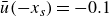 $\bar {u}(-x_s) = -0.1$
,
$\bar {u}(-x_s) = -0.1$
,
 $h(-x_s) = 1$
,
$h(-x_s) = 1$
,
 $Q = 1$
,
$Q = 1$
,
 $Q_{\textit{mom}}= 2$
,
$Q_{\textit{mom}}= 2$
,
 $N= 1$
, and a selection of
$N= 1$
, and a selection of
 $Q_{\textit{dip}}$
values:
$Q_{\textit{dip}}$
values:
 $Q_{\textit{dip}} =1.4$
(solid green),
$Q_{\textit{dip}} =1.4$
(solid green),
 $Q_{\textit{dip}} =1.532$
(dashed blue) and
$Q_{\textit{dip}} =1.532$
(dashed blue) and
 $Q_{\textit{dip}} =2$
(dash-dotted cyan). The bold black curve gives half-thicknesses satisfying the mass conservation condition and having a local magnitude of the Froude number equal to 1,
$Q_{\textit{dip}} =2$
(dash-dotted cyan). The bold black curve gives half-thicknesses satisfying the mass conservation condition and having a local magnitude of the Froude number equal to 1,
 $\mathcal{F}=1$
. Solutions in the region below this curve have
$\mathcal{F}=1$
. Solutions in the region below this curve have
 $\mathcal{F}\gt 1$
, and those in the region above it have
$\mathcal{F}\gt 1$
, and those in the region above it have
 $\mathcal{F}\lt 1$
.
$\mathcal{F}\lt 1$
.

To gain an insight into the solution structure for this quartic polynomial, thickness profiles are shown in figure 15 for a selection of parameter values. At each location
 $x$
, there are two, one or zero real solutions. Where there are two solutions, the upper solution branch has Froude number magnitude
$x$
, there are two, one or zero real solutions. Where there are two solutions, the upper solution branch has Froude number magnitude
 $\mathcal{F}(x)$
less than 1, while the lower branch has Froude number greater than 1 in magnitude. If there is only a single solution, then this solution has a Froude number of magnitude exactly 1. To form a solution valid across the source region, there are three distinct possibilities.
$\mathcal{F}(x)$
less than 1, while the lower branch has Froude number greater than 1 in magnitude. If there is only a single solution, then this solution has a Froude number of magnitude exactly 1. To form a solution valid across the source region, there are three distinct possibilities.
-
(i) The magnitude of the Froude number on both sides of the source is greater than 1. In this case,
$\mathcal{F}\gt 1$
throughout the source region, and the thickness profile must have
$h(x_0)=0$
for some
$x_0$
. -
(ii) The magnitude of the Froude number on one side of the source is greater than 1, and on the other side it is less than 1. In this case, the two solution branches must meet such that a transition between the upper and lower solution branches can occur. This is possible only at the origin.
-
(iii) The magnitude of the Froude number on both sides of the source is less than 1. In this case,
$\mathcal{F}\lt 1$
everywhere in the source region, and we follow the upper branch throughout.


Elaborating on the first case, we can explore the implications of enforcing
 $h(x_0)=0$
at some point in the domain. This condition implies
$h(x_0)=0$
at some point in the domain. This condition implies
 \begin{align} P_{1}(x_0) = \bar {u}(x_0)\,h(x_0) = 0 \quad \text{and} \quad P_{2}(x_0) = \bar {u}(x_0)^{2}\,h(x_0) + \frac {1}{3}N^{2}\, h(x_0)^{3} = 0. \end{align}
Now, for two positive real solutions of the polynomial to exist, Descartes’ rule of signs demands that
 \begin{align} P_{2}(x) \geqslant 0 \quad \text{for all }\quad |x|\leqslant x_s. \end{align}
Because we simultaneously require
 $P_{2}(x)$
to be greater than or equal to zero everywhere in the source region and for it to be equal to zero at
$P_{2}(x)$
to be greater than or equal to zero everywhere in the source region and for it to be equal to zero at
 $x_0$
,
$x_0$
,
 $x_0$
must be a minimum of
$x_0$
must be a minimum of
 $P_{2}$
since the function is piecewise linear. Looking at
$P_{2}$
since the function is piecewise linear. Looking at
 $\text{d}P_{2}(x)/\text{d}x$
, we have
$\text{d}P_{2}(x)/\text{d}x$
, we have
 \begin{align} \dfrac {\text{d}P_{2}(x)}{\text{d}x} = \begin{cases} \dfrac {1}{4}Q_{\textit{mom}} - \dfrac {1}{2}Q_{\textit{dip}} & \text{for }x\lt 0, \\[5pt] \dfrac {1}{4}Q_{\textit{mom}} + \dfrac {1}{2}Q_{\textit{dip}} & \text{for }x\gt 0. \end{cases} \end{align}
Thus for
 $|Q_{\textit{dip}}|\gt |Q_{\textit{mom}}|/2$
,
$|Q_{\textit{dip}}|\gt |Q_{\textit{mom}}|/2$
,
 $P_{2}(x)$
decreases to the left of zero, increases to the right of zero, and has an undefined gradient at
$P_{2}(x)$
decreases to the left of zero, increases to the right of zero, and has an undefined gradient at
 $x=0$
. This implies that the minimum of
$x=0$
. This implies that the minimum of
 $P_{2}(x)$
occurs at
$P_{2}(x)$
occurs at
 $x=x_0=0$
, and we must enforce
$x=x_0=0$
, and we must enforce
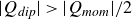 $|Q_{\textit{dip}}|\gt |Q_{\textit{mom}}|/2$
for meaningful solutions. Substituting
$|Q_{\textit{dip}}|\gt |Q_{\textit{mom}}|/2$
for meaningful solutions. Substituting
 $x_0=0$
back into the definitions of
$x_0=0$
back into the definitions of
 $P_{1}(x)$
and
$P_{1}(x)$
and
 $P_{2}(x)$
, we obtain the conditions
$P_{2}(x)$
, we obtain the conditions
 \begin{align} \bar {u}(-x_s)\,h(-x_s) = -\frac {1}{4}Q \quad \text{and} \quad \bar {u}(-x_s)^{2}\,h(-x_s) + \frac {1}{3}N^{2}\, h(-x_s)^{3} = -\frac {1}{4}Q_{\textit{mom}} + \frac {1}{2}Q_{\textit{dip}}. \end{align}
This yields half of the conditions required for specifying the source in the
 $\mathcal{F}\gt 1$
case. The remaining two conditions can be found by integrating across the full source domain:
$\mathcal{F}\gt 1$
case. The remaining two conditions can be found by integrating across the full source domain:
 \begin{align} \bar {u}(x_s)\, h(x_s) - \bar {u}(-x_s)\,h(-x_s) = \frac {1}{2}Q \end{align}
and
 \begin{align} \bar {u}(x_s)^{2}\, h(x_s) + \frac {1}{3}N^{2}\, h(x_s)^{3} - \bar {u}(-x_s)^{2}\,h(-x_s) - \frac {1}{3}N^{2}\, h(-x_s)^{3} = \frac {1}{2}Q_{\textit{mom}}. \end{align}
Note that these final two conditions are universal, regardless of the Froude number of the source, and indeed are all that is required if
 $\mathcal{F}\lt 1$
on both sides of the source. In this case, the flow is in a buoyancy-dominated regime, and information from the fronts can propagate against the flow to the source, meaning that less information is required from the source to specify the system.
$\mathcal{F}\lt 1$
on both sides of the source. In this case, the flow is in a buoyancy-dominated regime, and information from the fronts can propagate against the flow to the source, meaning that less information is required from the source to specify the system.
Moving on to the second case, in which the magnitude of the Froude number is less than 1 on one side of the source, and greater than 1 on the other, we now consider conditions under which the upper and lower branches touch. For this to occur, the curves must intersect at the origin (for an example, see the green curve in figure 15) and
 $\mathcal{F}(0)=1$
. These conditions are sufficient to specify the system in this case. Explicitly, they imply
$\mathcal{F}(0)=1$
. These conditions are sufficient to specify the system in this case. Explicitly, they imply
 \begin{align} \bar {u}(0)\, h(0) = \bar {u}(-x_s)\,h(-x_s) + \frac {1}{2}Q \end{align}
and
 \begin{align} \bar {u}(0)^{2}\,h(0) + \frac {1}{3}N^{2}\, h(0)^{3} = \bar {u}(-x_s)^{2}\,h(-x_s) + \frac {1}{3}N^{2}\, h(-x_s)^{3} +\frac {1}{4}Q_{\textit{mom}} - \frac {1}{2}Q_{\textit{dip}}, \end{align}
which in conjunction with (B14) and (B15) specify the source in this case.
Translating these conditions into similarity form, we finally obtain the following conditions. If
 $\mathcal{F}_s\lt1$
on both sides of the source, then the only conditions required are given by (4.2) in the main text. If
$\mathcal{F}_s\lt1$
on both sides of the source, then the only conditions required are given by (4.2) in the main text. If
 $\mathcal{F}_s\gt 1$
on one side of the source, then the additional conditions
$\mathcal{F}_s\gt 1$
on one side of the source, then the additional conditions
 \begin{align} \left [\mathcal{U}\mathcal{H}\right ]_{0^-}^{0} = \frac {1}{4} \quad \text{and} \quad \left [\mathcal{U}^2\mathcal{H} + \frac {1}{3}\mathcal{H}^3\right ]_{0^-}^{0} = \frac {1}{4}\frac {\textit{NQ}_{\textit{mom}} }{(\textit{NQ})^{3/2}} - \frac {1}{2}\frac {\textit{NQ}_{\textit{dip}} }{(\textit{NQ})^{3/2}} \end{align}
are required. Finally, if
 $\mathcal{F}_s\gt 1$
on both sides, then
$\mathcal{F}_s\gt 1$
on both sides, then
 \begin{align} \mathcal{H} =0 \quad \text{at } \eta =0 \end{align}
must also be imposed. In this case, the fluid in essence is being ejected at such speed in both directions that a dry spot develops in the middle of the source.
B.4. Parameter space
Figure 16 shows the type of solution in each region of
 $(\beta ,Q_{\textit{dip}} )$
parameter space for a quiescent ambient, together with representative thickness and velocity profiles. Here, we allow
$(\beta ,Q_{\textit{dip}} )$
parameter space for a quiescent ambient, together with representative thickness and velocity profiles. Here, we allow
 $\beta$
to be an arbitrary constant to illustrate the range of possible behaviours. Parameter values for which the solution structure is independent of the source details (in other words,
$\beta$
to be an arbitrary constant to illustrate the range of possible behaviours. Parameter values for which the solution structure is independent of the source details (in other words,
 $\mathcal{F}_s\leqslant 1$
on both side of the source) are shaded. Where ambient resistance to propagation is high (
$\mathcal{F}_s\leqslant 1$
on both side of the source) are shaded. Where ambient resistance to propagation is high (
 $\beta \lt 1$
) and the source is relatively weak (
$\beta \lt 1$
) and the source is relatively weak (
 $Q_{\textit{dip}}$
is small), solutions are type C-C with a uniform thickness profile and a constant velocity on each side of the source. Where ambient resistance is lower (
$Q_{\textit{dip}}$
is small), solutions are type C-C with a uniform thickness profile and a constant velocity on each side of the source. Where ambient resistance is lower (
 $\beta \gt 1$
), solutions are type RC-RC for weak sources, and type CRC-CRC for moderate sources. In either case, the intrusion can propagate easily into the ambient fluid, and the fluid accelerates and thins away from the source. Finally, for strong sources (
$\beta \gt 1$
), solutions are type RC-RC for weak sources, and type CRC-CRC for moderate sources. In either case, the intrusion can propagate easily into the ambient fluid, and the fluid accelerates and thins away from the source. Finally, for strong sources (
 $Q_{\textit{dip}}$
large), solutions become type CSC-CSC for all finite
$Q_{\textit{dip}}$
large), solutions become type CSC-CSC for all finite
 $\beta$
: fluid is ejected from the source as a thin, fast jet that thickens and slows through a shock to a buoyancy-dominated frontal region controlled by ambient resistance to propagation.
$\beta$
: fluid is ejected from the source as a thin, fast jet that thickens and slows through a shock to a buoyancy-dominated frontal region controlled by ambient resistance to propagation.
Similarity solutions of the intrusive shallow-water model for a constant source and a quiescent ambient
 $U_a=0$
,
$U_a=0$
,
 $Q_{\textit{mom}} =0$
. The main panel shows the type of solution as a function of frontal Froude number
$Q_{\textit{mom}} =0$
. The main panel shows the type of solution as a function of frontal Froude number
 $\beta$
and source dipole strength
$\beta$
and source dipole strength
 $Q_{\textit{dip}}$
. In the shaded region, solutions exterior to the source are independent of the value of
$Q_{\textit{dip}}$
. In the shaded region, solutions exterior to the source are independent of the value of
 $Q_{\textit{dip}}$
. The hashed region represents realistic values of the frontal Froude number in the model of Ungarish (Reference Ungarish2005). The plots show the scaled self-similar thickness profiles
$Q_{\textit{dip}}$
. The hashed region represents realistic values of the frontal Froude number in the model of Ungarish (Reference Ungarish2005). The plots show the scaled self-similar thickness profiles
 $Nh/\sqrt{\textit{NQ}}$
(solid) and velocity profiles
$Nh/\sqrt{\textit{NQ}}$
(solid) and velocity profiles
 $\bar {u}/\sqrt{\textit{NQ}}$
(dashed) at the parameter values indicated.
$\bar {u}/\sqrt{\textit{NQ}}$
(dashed) at the parameter values indicated.

This latter case provide some rationalisation for the behaviour in the diffuser-generated experiments. In these experiments, the momentum source is strong, and the corresponding theoretical solutions include a shock. These are indeed observed, although experimentally there is significant entrainment across the shock; this effect is not accounted for in the model, so the detailed predictions are not valid and are not discussed further.


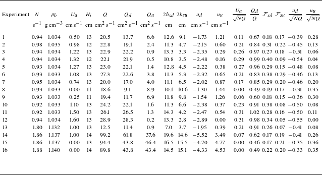


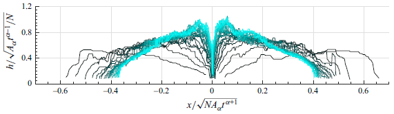

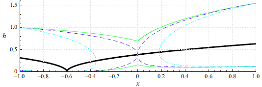


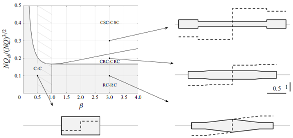


 Open access