


I. Introduction
Very large and dominant “superstar” firms have a significant and sometimes disproportionate impact on various macroeconomic outcomes. In particular, these firms dominate exports, foreign direct investment, and research and development, which in turn has generated a sharp increase in their profits and an increased industry concentration in the United States (Autor, Dorn, Katz, Patterson, and Van Reenen (Reference Autor, Dorn, Katz, Patterson and Van Reenen2017), Grullon, Larkin, and Michaely (Reference Grullon, Larkin and Michaely2019), De Loecker, Eeckhout, and Unger (Reference De Loecker, Eeckhout and Unger2020)).Footnote 1 The recent growth in artificial intelligence technologies has further emphasized superstar firms’ importance (Babina, Fedyk, He, and Hodson (Reference Babina, Fedyk, He and Hodson2024)). These firms also play a significant role in aggregate macroeconomic fluctuations (Gabaix (Reference Gabaix2011), Jannati, Korniotis, and Kumar (Reference Jannati, Korniotis and Kumar2020)).
The rise and dominance of star firms can be attributed to several economic factors, including economies of scale, increasing importance of proprietary information technology (Bessen (Reference Bessen2020)), accumulation of intangible digital capital (Tambe, Hitt, Rock, and Brynjolfsson (Reference Tambe, Hitt, Rock and Brynjolfsson2020)), easier access to human capital (Choi, Lou, and Mukherjee (Reference Choi, Lou and Mukherjee2026)), and weakening antitrust enforcement (Döttling, Gutiérrez, and Philippon (Reference Döttling, Gutierrez and Philippon2017)). As large firms attain star status, they can use their market power to create barriers to entry. Because star firms influence the broader economy and industries around them, changes in their operational and earnings performance can predict changes in the future earnings and performance of other related firms. Further, if market participants, such as sell-side equity analysts, do not fully account for this dynamic, it can create predictable patterns in related firms’ earnings surprises and returns.
In this article, we extend and complement the extant literature on star firms to investigate the financial and economic information spillovers of star firms within industries. Our analysis adopts the industry star firm definition developed by Gutiérrez and Philippon (Reference Gutiérrez and Philippon2019), who classify industry stars as the four largest firms by market capitalization within each of the 60 Bureau of Economic Analysis (BEA) industries. We find that performance shifts of these star firms predict future earnings growth and stock returns of connected nonstar firms, as well as future GDP and employment growth at the industry level. We also investigate the intra-industry mechanisms underlying these spillover effects and assess whether sell-side analysts fully incorporate the information from star firms into their earnings forecasts.
Background on star firms. The Gutiérrez and Philippon (Reference Gutiérrez and Philippon2019) industry star firms are typically large but not all large firms qualify as stars. Based on descriptive statistics, the industry star firms differ from large nonstar firms along several characteristics associated with superstar firms in the previous literature. Defining large nonstars as firms in the top 30% of industry market capitalization, we find that industry stars are more profitable, have higher R&D and capital expenditure, and are more innovative based on the number of patents.Footnote 2
The industry-level star firm definition of Gutiérrez and Philippon (Reference Gutiérrez and Philippon2019) offers several advantages for our study. First, their classification avoids concentration in any single industry, ensuring that our results are not driven by industry-specific factors. Second, sell-side security analysts typically specialize in specific industries, meaning the same analysts often issue forecasts for both star and nonstar firms within an industry. Third, the number of star firms and industries remains constant over time, which aids in interpreting the empirical results.
Predictability of nonstar earnings. We start our empirical analysis by documenting that changes in star firms’ relative earnings performance predict the earnings growth of same-industry nonstar firms. To measure the relative earnings performance of star and nonstar firms, we create a measure called ΔEGP Difference that captures the relative earnings growth difference between star and nonstar firms within the same industry. Specifically, ΔEGP Differencet−1 captures the change in the difference between star and nonstar firms’ average earnings growth between quarters t−1 and t−2. Earnings Growth (EGP) in quarter t is defined as earnings per share in quarter t minus earnings in quarter t−4, scaled by the share price. ΔEGP Difference is high (low) when star firms’ earnings growth relative to nonstar firms’ earnings growth is higher (lower) in the current quarter than in the previous quarter. Intuitively, it obtains high values when star firms’ earnings growth increases relative to nonstar firms across quarters.
The conjecture that the ΔEGP Difference measure captures information about current and future firm performance is supported by the results of He and Narayanamoorthy (Reference He and Narayanamoorthy2020). They find that earnings growth acceleration, defined as quarter-over-quarter change in earnings growth, has explanatory power for future excess returns.Footnote 3 Their earnings growth measure is identical to ours, and another interpretation for the ΔEGP Difference variable is that it captures the difference in earnings growth acceleration between star and nonstar firms.Footnote 4
We estimate quarterly industry-level panel regressions of average earnings growth for star and nonstar firms on ΔEGP Differencet−1, controlling for lagged dependent variables and including year-quarter and industry fixed effects. For nonstar firms, one-quarter lagged ΔEGP Difference significantly predicts earnings growth, with coefficients between 0.10 and 0.19 and t-values from 3.9 to 5.1. These estimates imply that a 1-standard-deviation increase in ΔEGP Differencet−1 corresponds to a 0.1–0.2-standard-deviation increase in nonstar firms’ earnings growth. By contrast, the coefficients in regressions for star firms are negative and insignificant. This contrast suggests that changes in star firms’ relative earnings performance predict future earnings growth of nonstar firms but not of star firms themselves.
Evidence on economic channels. We also examine the economic channels that may drive the earnings growth spillover effect. One mechanism supported by empirical evidence is a price markup spillover, where star firms’ markup changes influence nonstars’ markups and profit margins. This can occur if star firms act as price setters due to their market power, while nonstars follow as price takers. Consistent with this channel, an earnings growth decomposition analysis shows that the earnings growth component driven by profit margin changes is most sensitive to shifts in ΔEGP Difference. Using a detailed price markup measure developed by De Loecker, Eeckhout, and Unger (Reference De Loecker, Eeckhout and Unger2020), we also find that star firms’ markup changes predict nonstars’ markup changes at the annual level.
Other channels are also supported by the data. Cross-industry analyses show that earnings predictability is stronger in industries with high technology spillovers and greater vertical integration, suggesting that stars’ roles as innovation leaders and supply chain anchors can contribute to the effect. Notably, while our results indicate that ΔEGP Difference predicts changes in profit margin-driven earnings growth, we find that this effect is limited to improvements in operating income relative to cost of goods sold. These findings suggest that technology spillovers are more likely associated with product innovation than with broader operational efficiency gains, which would be reflected in other components of the profit margin.
Predictability of industry GDP and employment. Beyond earnings growth, we find that star firms’ performance shifts, captured by ΔEGP Difference, also predict broader industry-level economic outcomes. First, we test whether ΔEGP Difference can forecast changes in nonstar firms’ quarterly job postings, which are a timely indicator of firms’ growth and growth prospects. Industry-level panel regressions show that a 1-standard-deviation increase in lagged ΔEGP Difference predicts a 34% increase in nonstar firms’ job postings and the coefficient is statistically significant. We also find that ΔEGP Difference predicts industry-level real GDP and employment growth. Specifically, a 1-standard-deviation increase in lagged ΔEGP Difference is associated with a 0.5–0.6 percentage point rise in industry GDP growth and a 0.1–0.2 percentage point rise in employment growth, both statistically significant at the 10% level or higher. Importantly, these figures capture the broader industry impact, including nonlisted firms.
As further evidence of star firms’ information spillovers related to economic growth, we find that the percentage change in star firms’ price-to-earnings (P/E) ratio can statistically significantly predict industry GDP growth changes at the annual level. P/E ratios reflect market expectations about long-term growth opportunities, and our results are consistent with findings by Bekaert, Harvey, Lundblad, and Siegel (Reference Bekaert, Harvey, Lundblad and Siegel2007), who show that a country’s growth opportunities, measured by its industry mix valued at global P/E ratios, can predict country-specific GDP growth.
Predictability of earnings surprises. In the next set of tests, we examine whether security analysts use the information reflected in star firms’ relative earnings growth to update their earnings forecasts. Our conjecture is that sell-side equity analysts may not be completely aware of the information spillovers from star firms. As a result, they would not fully account for the information content in star firms’ earnings, and consequently, the ΔEGP Difference variable would predict the consensus earnings surprises of nonstar firms.
To test this conjecture, we regress nonstar firms’ average quarterly consensus forecast-based earnings surprise at the industry level on lagged ΔEGP Difference. The regressions include the same control variables as our previous earnings growth regressions, and we additionally estimate specifications that control for lagged consensus-based earnings surprises. Consistent with our conjecture, we find that the coefficient on ΔEGP Difference is positive and statistically significant (coefficient estimate = 0.015, t-value = 2.5), indicating that analysts underreact to the information content in star firms’ earnings surprises. Based on the coefficient estimates, a 1-standard-deviation change in ΔEGP Difference corresponds to a 0.1-standard-deviation increase in the dependent variable.
Consistent with the earnings surprise results, we also find that the ΔEGP Difference can predict nonstar firms’ abnormal returns around earnings announcements. The ΔEGP Difference coefficient estimates in similar regressions explaining nonstars’ cumulative abnormal returns over the [0, 2] day window are positive and statistically significant with a coefficient value of 0.07. In contrast, the coefficient estimates in star firm regressions are negative and statistically insignificant.
Return predictability. In the last set of tests, we demonstrate that our core findings have pricing implications. Specifically, using a long–short industry portfolio strategy, we analyze whether star firms’ earnings performance can predict the monthly cross-sectional stock returns of nonstar firms. To have a higher-frequency measure of earnings performance shifts, we calculate ΔEGP Difference every month based on earnings announcements in months t−1 to t−3 and denote this as ΔEGP Difference Monthly. We create monthly market value-weighted quintile portfolios of industries with the highest and lowest lagged values of ΔEGP Difference Monthly. Our long portfolio invests in the 11 highest-ranked industry portfolios and the short portfolio invests in the 11 lowest-ranked industry portfolios. These correspond to the top and bottom quintile within the 55 industries for which we have sufficient observations.
We find that star firms’ relative earnings performance contains information that is not fully incorporated into market prices and can therefore predict future stock returns. The long–short portfolio earns an average monthly 6-factor alpha of 0.73%, which is statistically significant with a t-statistic of 2.35. In line with these results, we also find that there is a lead–lag relation between star firms’ and nonstar firms’ stock returns. We form market value-weighted quintile portfolios of nonstar firms in industries with the highest and lowest lagged average stock return of star firms in the previous month. A long–short investment strategy based on these portfolios earns a monthly 6-factor alpha of 0.47% with a t-statistic of 2.41.
Finally, we analyze whether the information spillovers of star firms are unique or simply reflect general large-firm effects. We replicate our main analyses using the four next-largest firms in each industry as “substitute” stars. While ΔEGP Difference based on these substitutes still predicts nonstars’ earnings growth, the effect is only approximately half as large as that of actual stars. Moreover, the substitutes do not significantly predict outcomes related to analyst forecasts or stock returns. All coefficients for nonstar earnings surprises, earnings announcement returns, and abnormal returns are statistically insignificant. These placebo tests confirm that the spillover effects we observe are specific to star firms and not just a feature of large firms in general.
Connections to the literature. Together, these results contribute to several strands of accounting, economics, and finance literature. We provide novel market- and operating-performance-based evidence that shifts in star firms’ earnings performance can predict future outcomes of related firms. The industry-level GDP and employment results show that these spillovers extend beyond firm performance to broader economic outcomes, linking to prior work that uses accounting data to forecast macroeconomic indicators such as GDP and employment.Footnote 5 We show that a leading indicator based on a small group of star firms can predict industry growth and activity. Our analysis using stars’ P/E ratios to predict industry GDP growth changes also connects to Bekaert et al. (Reference Bekaert, Harvey, Lundblad and Siegel2007), who use countries’ industry mix and global P/E ratios to predict their future growth.
The results with the ΔEGP Difference variable extend the earnings acceleration results of He and Narayanamoorthy (Reference He and Narayanamoorthy2020) by demonstrating that the relative earnings acceleration of star firms can predict other firms’ future earnings and stock returns. Earnings growth acceleration is less salient than year-over-year earnings growth, which can result in underreaction among security analysts and market participants.
Finally, our return results also add to the literature on lead–lag effects in stock returns.Footnote 6 We identify a new lead–lag pattern where star firms’ earnings and stock return performance predict the returns and earnings surprises of other connected firms. In related work, Hou (Reference Hou2007) finds that the returns of the largest firms in an industry lead the returns of the smallest firms in an industry.Footnote 7 We discover a similar lead–lag pattern, but our “lag” sample is not limited to small firms, and only some of the large firms are classified as star firms in the “lead” sample.
II. Data Sources and Variables
A. Data Sources
We use stock price and stock return data from the CRSP database, financial information from Compustat, and analysts’ quarterly earnings forecasts and associated earnings information from the IBES detail history file. The earnings per share (EPS) values are from IBES (Item Actual), and they are adjusted for stock splits using item CFACPR in CRSP. We adjust the CRSP returns for delisting following the procedure of Shumway (Reference Shumway1997). In analyses that involve earnings announcement dates, we limit the sample to post-1993 observations due to known data errors in the early years covered by IBES. The sample period for analyses that only use stock return data is 1984 to 2020.
We apply multiple filters to address data errors and potential concerns about data quality. We require the date on which an analyst forecast becomes effective (ACTDATS) to be on or after the analyst forecast announcement date (ANNDATS), and the forecast review date (REVDATS) should be after the forecast announcement date (ANNDATS). We further require at least two analysts covering a stock each quarter and at least two firms covered by sample analysts. Last, we exclude firms with prices below $1 to ensure that our results are not driven by illiquid firms.
In our job posting analyses, we use job posting data from LinkUp, a vendor that collects postings directly from company websites, covering nearly 160 million advertised positions. Campello, Kankanhalli, and Muthukrishnan (Reference Campello, Kankanhalli and Muthukrishnan2024) show that LinkUp data are representative of corporate hiring in the United States.Footnote 8 The data include the title, job description, company information, geographic location, creation date, and O*NET job classification code for the postings. The original LinkUp data set covers 163,171,800 job postings from August 2007 to May 2022. After excluding job postings of private firms and those with missing information, our final sample consists of 671,084 observations, including 3,515 firms from 2008 to 2020. We aggregate the job postings at the industry level to create industry-level job postings variables for star and nonstar firms, respectively.
We utilize quarterly and annual industry-level real GDP data from the Bureau of Economic Analysis (BEA). The quarterly data set spans from 2005 to 2020, while the annual sample covers our full sample period from 1984 to 2020.Footnote 9 Additionally, we source industry-level employment data from the Bureau of Labor Statistics (BLS), covering the period from 1993 to 2020. We use the North American Industry Classification System (NAICS) industry codes to merge BEA and BLS data sets with our sample. In instances where industry-level real GDP or employment data are unavailable for our specific industry definitions, we aggregate the quarterly figures for subindustries to align them with our industry classifications.
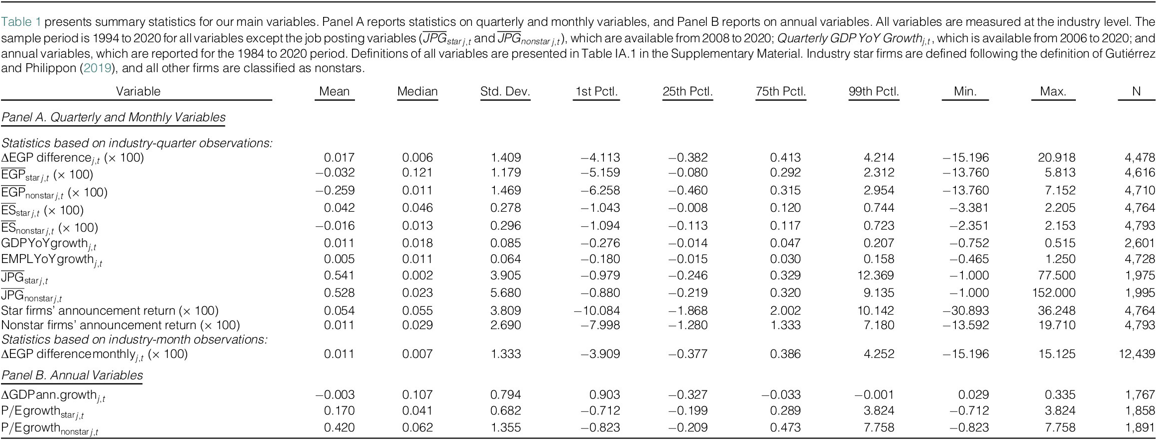
Lastly, we use several databases provided by other researchers. We use patent counts and citations from the Kogan, Papanikolaou, Seru, and Stoffman (Reference Kogan, Papanikolaou, Seru and Stoffman2019) depositoryFootnote 10 and price markup data from De Loecker et al. (Reference De Loecker, Eeckhout and Unger2020). Firm-level Technology Spillover scores are sourced from the Bloom, Schankerman, and Van Reenen (Reference Bloom, Schankerman and Van Reenen2013) depository (https://nbloom.people.stanford.edu/research), while pairwise Vertical Integration scores come from the Vertical TNIC (VTNIC) database developed by Frésard, Hoberg, and Phillips (https://faculty.marshall.usc.edu/Gerard-Hoberg/FresardHobergPhillipsDataSite/index.html (Reference Frésard, Hoberg and Phillips2020)). Finally, monthly factor return data are obtained from the Kenneth French data library (https://mba.tuck.dartmouth.edu/pages/faculty/ken.french/data_library.html). Table 1 reports descriptive statistics for key variables used in the analyses.
B. Defining Star Firms
To identify dominant star firms at the industry level, we use the industry star definition of Gutiérrez and Philippon (Reference Gutiérrez and Philippon2019). They define star firms as top four firms by the market value of equity within each BEA industry.Footnote 11 BEA follows the NAICS classification for grouping firms into industries. We use NAICS codes from Compustat to match firms with their corresponding BEA industry classification.
Following Gutiérrez and Philippon (Reference Gutiérrez and Philippon2019), we rank all firms within an industry by their market capitalization at the end of December each year and specify the top four as star firms for the following year. In cases of missing CRSP market capitalization data, we use Compustat to calculate the values. If both sources are unavailable, we fill in the missing market capitalization ranks with firms’ net sales (Compustat item SALE) ranks within each industry.Footnote 12
Table IA.2 in the Supplementary Material presents the percentage of market capitalization of star and nonstar firms within the 60 BEA industry groups. We exclude five industry groups due to insufficient observations because we require at least five nonstar firms in the industry each month. These five industries are presented in Table IA.2 in the Supplementary Material with 0 observations. The average number of nonstar firms ranges from 5 to 543 in industries with stars. Star status is persistent, and 83% of star firms were also star firms in the previous year.
C. Star Firms Versus Large Firms
Summary statistics indicate that the Gutiérrez and Philippon (Reference Gutiérrez and Philippon2019) star firms differ from other large firms in their profitability, investment activities, and innovativeness. Table 2 compares the characteristics of star firms and nonstar large firms. We define “large firms” following the definition of Hou (Reference Hou2007), who classifies them as those belonging to the 30% of market capitalization in each industry.
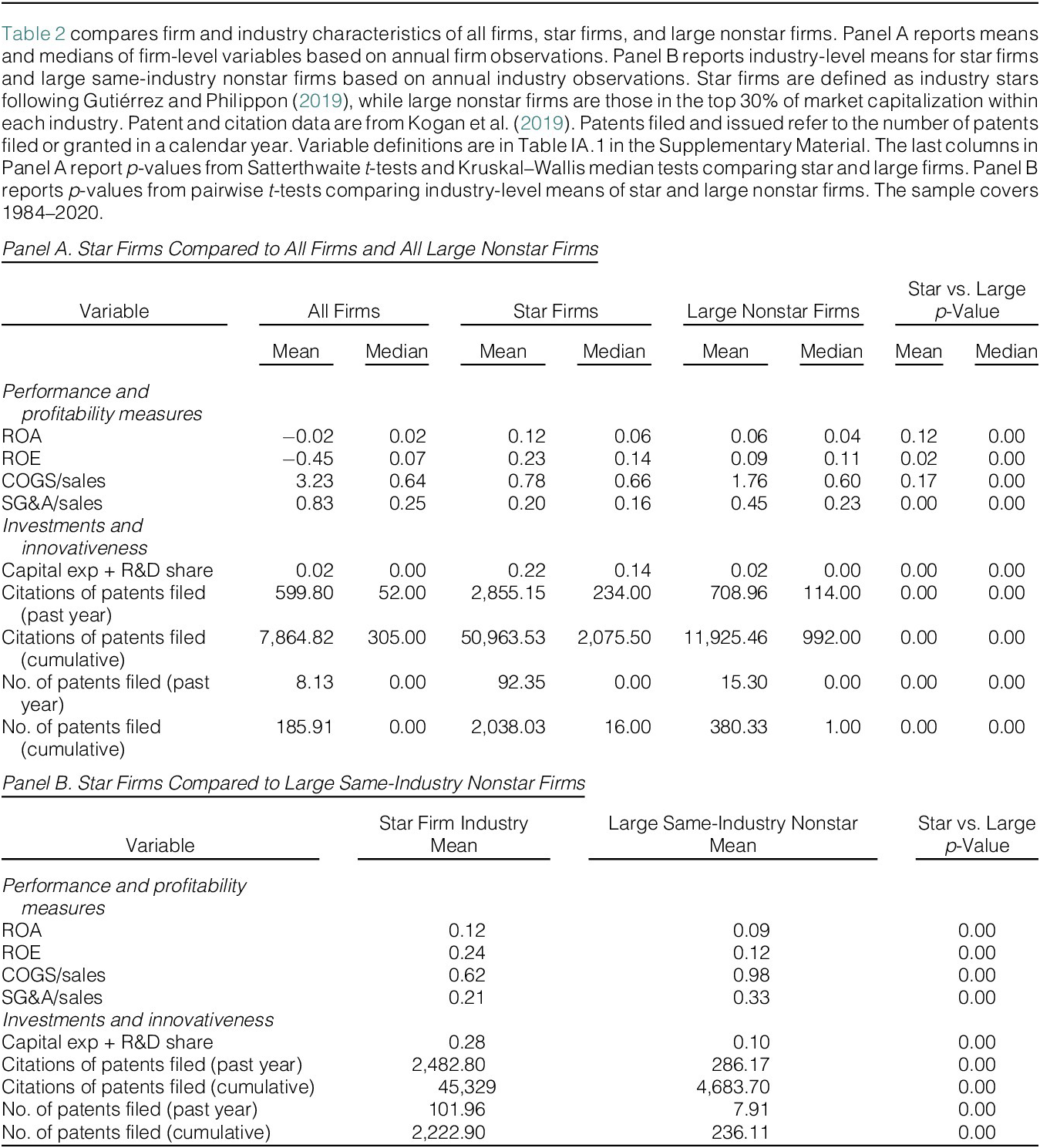
Star firms are more profitable based on their Return on Assets (ROA) and Return on Equity (ROE). The median ROA of star firms is 6%, which is 50% higher than large nonstars’ median ROA of 4% (means are 12% and 6%, respectively). They also have lower cost of goods sold and nonproduction expenses relative to sales, which is consistent with economies of scale. We find that star firms are more innovative and research-oriented than typical large firms, as measured by the share of total capital and R&D expenditure in the industry and the number of patents. Star firms file an average of 92.35 patents per year, as compared to 15.30 patents by large nonstar firms. Panel B shows that there is also a statistically significant difference in means of all these characteristics when we compare star firms with large nonstar firms that are within the same industry.
D. Measuring Relative Earnings Performance and Earnings Surprises
To measure relative earnings performance, we define a variable denoted as ΔEGP Differencej,t, which captures quarterly changes in the earnings growth difference between star and nonstar firms. It is defined as follows:
 $$ {\varDelta EGP\ Difference}_{j,t}=\left({{\overline{EGP}}_{star}}_{j,t}-{{\overline{EGP}}_{nonstar}}_{j,t}\right)-\left({{\overline{EGP}}_{star}}_{j,t-1}-{{\overline{\; EGP}}_{nonstar}}_{j,t-1}\right), $$
where $ {{\overline{EGP}}_{star}}_{j,t} $
and
$ {{\overline{EGP}}_{star}}_{j,t} $
and $ {{\overline{EGP}}_{nonstar}}_{j,t} $
refer to the equal-weighted average earnings growth (EGP) of star firms and nonstar firms in industry j in quarter t, respectively. EGP is a measure of earnings growth for each firm i and, following previous related studies, we define it as the earnings per share (EPS) in quarter t minus EPS in quarter t–4, scaled by share price 10 days before the earnings announcement date. Specifically,
$ {{\overline{EGP}}_{nonstar}}_{j,t} $
refer to the equal-weighted average earnings growth (EGP) of star firms and nonstar firms in industry j in quarter t, respectively. EGP is a measure of earnings growth for each firm i and, following previous related studies, we define it as the earnings per share (EPS) in quarter t minus EPS in quarter t–4, scaled by share price 10 days before the earnings announcement date. Specifically,
 $$ {EGP}_{i,t}=\frac{EPS_{i,t}-{EPS}_{i,t-4}}{Price_{i,t}}. $$
We define ΔEGP Difference for industry-quarter observations where the industry has at least five nonstar firms in addition to star firms. This measure is based on a change in the difference between star and nonstar firms’ earnings growth, and intuitively, it obtains high values when star firms’ earnings growth across quarters increases relative to same-industry nonstar firms. Measuring the change in earnings growth difference between quarters ensures that we are not capturing differences in long-term trends between stars and nonstars.
Our measure is motivated by the results of He and Narayanamoorthy (Reference He and Narayanamoorthy2020), who find that earnings growth acceleration defined as quarter-over-quarter change in earnings growth ( $ {EGP}_{i,t} $
) predicts companies’ future excess returns and earnings growth. They argue that this earnings acceleration anomaly is attributable to the market missing, at least partially, the implications of earnings acceleration for earnings growth 2 and 3 quarters in the future. Our ΔEGP Differencej,t can also be interpreted as the difference between star firms’ and nonstar firms’ earnings growth acceleration over the previous quarter according to their measure. Formally,
$ {EGP}_{i,t} $
) predicts companies’ future excess returns and earnings growth. They argue that this earnings acceleration anomaly is attributable to the market missing, at least partially, the implications of earnings acceleration for earnings growth 2 and 3 quarters in the future. Our ΔEGP Differencej,t can also be interpreted as the difference between star firms’ and nonstar firms’ earnings growth acceleration over the previous quarter according to their measure. Formally, $ {\varDelta EGP\ Difference}_{j,t} $
can also be expressed as
$ {\varDelta EGP\ Difference}_{j,t} $
can also be expressed as $ \left({{\overline{EGP}}_{star}}_{j,t}-{{\overline{EGP}}_{star}}_{j,t-1}\right)-\left({{\overline{EGP}}_{nonstar}}_{j,t}-{{\overline{\; EGP}}_{nonstar}}_{j,t-1}\right) $
, which is simply star firms’ earnings growth acceleration minus that of nonstar firms under the He and Narayanamoorthy (Reference He and Narayanamoorthy2020) definition.Footnote
13
$ \left({{\overline{EGP}}_{star}}_{j,t}-{{\overline{EGP}}_{star}}_{j,t-1}\right)-\left({{\overline{EGP}}_{nonstar}}_{j,t}-{{\overline{\; EGP}}_{nonstar}}_{j,t-1}\right) $
, which is simply star firms’ earnings growth acceleration minus that of nonstar firms under the He and Narayanamoorthy (Reference He and Narayanamoorthy2020) definition.Footnote
13
For stock return predictability tests, we create a monthly measure of relative earnings performance called ΔEGP Difference Monthlyj,t−1. Footnote 14 This is similar to the quarterly ΔEGP Differencej,t measure, except that it is updated monthly based on earnings announcements within the past 3 months. This higher frequency allows us to predict returns using the most recent earnings information available to market participants. For a firm to be included in the ΔEGP Difference Monthlyj,t calculation each month, it needs to have nonmissing EGP observations at least during the past 2 quarters.
Last, we construct measures of analyst earnings surprise for star and nonstar firms. We compute each firm’s analyst earnings surprise ( $ {ES}_{i,t} $
) as (EPSi,t – Consensus Forecasti,t)/ Pricei,t
$ {ES}_{i,t} $
) as (EPSi,t – Consensus Forecasti,t)/ Pricei,t $ , $
where EPSi,t, Consensus Forecast
i,t
, and Price
i,t
are firm i’s actual EPS, analysts’ median forecast, and share price 10 days before the earnings announcement date, respectively. We take the average earnings surprise of star and nonstar firms in each industry j and quarter t to achieve industry-level measures of earnings surprise for star and nonstar firms, that is,
$ , $
where EPSi,t, Consensus Forecast
i,t
, and Price
i,t
are firm i’s actual EPS, analysts’ median forecast, and share price 10 days before the earnings announcement date, respectively. We take the average earnings surprise of star and nonstar firms in each industry j and quarter t to achieve industry-level measures of earnings surprise for star and nonstar firms, that is, $ {{\overline{ES}}_{star}}_{j,t} $
and
$ {{\overline{ES}}_{star}}_{j,t} $
and $ {{\overline{ES}}_{nonstar}}_{j,t} $
, respectively.
$ {{\overline{ES}}_{nonstar}}_{j,t} $
, respectively.
Panel A of Table 1 presents summary statistics for all our earnings measures described earlier. The earnings performance variables ΔEGP Differencej,t and ΔEGP Difference Monthlyj,t have almost identical distributions with means and medians close to 0. Specifically, the mean of ΔEGP Differencej,t is 0.017 and has a median of 0.006. A variance decomposition analysis indicates that over 99% of the variation in ΔEGP Differencej,t is attributable to differences across industries rather than within industries.Footnote 15
III. Star Firms and Industry Spillover Effects
We begin by testing whether shifts in star firms’ relative earnings performance, as measured by ΔEGP Difference, can predict the earnings growth of other related firms. We then extend the analysis to job postings and industry-level employment and GDP growth.
A. Predicting Earnings Growth: Baseline Results
We estimate quarterly panel regressions where the dependent variable is either the average earnings growth of nonstar firms or star firms within industry j during quarter t. The key independent variable is ΔEGP Differencej,t−1. These regressions control for lagged values of the dependent variable (i.e., $ \overline{EGP} $
j,t − 1,
$ \overline{EGP} $
j,t − 1, $ \overline{EGP} $
j,t − 2, and
$ \overline{EGP} $
j,t − 2, and $ \overline{EGP} $
j,t−3) and include year-quarter and industry fixed effects. The fixed effects control for all common industry- and time-specific factors that potentially affect the earnings growth of star and nonstar firms.
$ \overline{EGP} $
j,t−3) and include year-quarter and industry fixed effects. The fixed effects control for all common industry- and time-specific factors that potentially affect the earnings growth of star and nonstar firms.
Table 3 reports the earnings growth predictability regression estimates. In columns 1–3, we report the panel regression results for nonstar firms, and columns 4–6 report the results for star firms. Our conjecture is that ΔEGP Differencej,t−1 would predict earnings growth of nonstar firms, as star firms’ relative earnings performance changes are likely to contain useful information about nonstar firms’ future earnings performance.
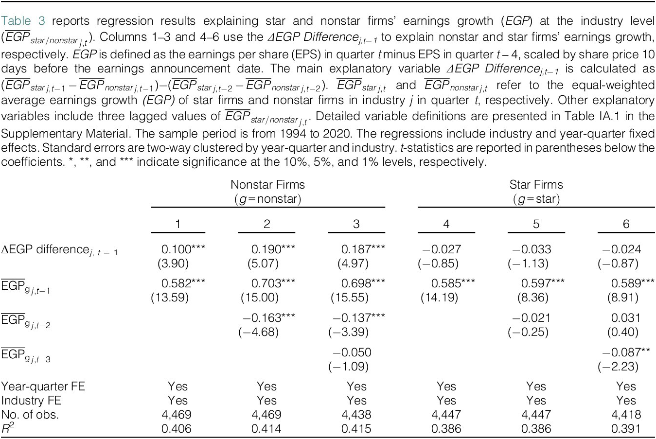
The estimates in columns 1–3 of Table 3 confirm our conjecture. ΔEGP Differencej,t−1 can predict nonstar firms’ earnings growth in the same industry, after controlling for lagged earnings growth of nonstar firms. The coefficients on ΔEGP Difference are between 0.100 and 0.190 with t-statistics between 3.90 and 5.07, respectively. In terms of economic magnitude, these coefficient estimates imply that a 1-standard-deviation increase in ΔEGP Differencej,t−1 is associated with a 0.1- to 0.2-standard-deviation increase in the earnings growth of nonstar firms.
To rule out the possibility that ΔEGP Differencej,t−1 captures general industry information that affects stars and nonstars equally, in columns 4–6, we re-estimate the earnings regressions so that we form the dependent variable based on star firms instead of nonstar firms. We find that ΔEGP Differencej,t−1 is unable to predict the earnings growth of star firms. Specifically, the coefficients on ΔEGP Differencej,t−1 are in the range of −0.024 to −0.033, and they are statistically and economically insignificant. These results show that information in earnings growth of star firms, rather than industry and time trends, predicts the earnings growth of nonstar firms.
B. Earnings Growth Spillover: Additional Analyses and Robustness Checks
We conduct several checks and additional analyses to verify that our results are robust to alternative specifications. To ensure that the results are not affected by outlier observations, Table IA.3 in the Supplementary Material repeats the analyses of Table 3 using a sample where ΔEGP Differencej,t−1 is truncated at the 1% and 99% levels across the panel, and the results remain similar. We also verify that ΔEGP Differencej,t−1 can predict nonstars’ earnings growth at the firm level. Columns 1–3 of Table IA.4 in the Supplementary Material report results from firm-level regressions that correspond to columns 1 to 3 of Table 3. All the ΔEGP Differencej,t−1 coefficients are positive and statistically significant.Footnote 16
For additional robustness, we repeat our tests using alternative measures of relative earnings performance. First, we define relative earnings performance by using the quarterly difference in earnings growth, without any detrending. Instead of using ΔEGP Differencej,t−1 (see equation (1)), we use the lagged difference $ \left({{\overline{EGP}}_{star}}_{j,t-1}-{{\overline{EGP}}_{nonstar}}_{j,t-1}\right) $
. The regression estimates are reported in Table IA.5, Panel A in the Supplementary Material. We find that our results remain qualitatively similar.
$ \left({{\overline{EGP}}_{star}}_{j,t-1}-{{\overline{EGP}}_{nonstar}}_{j,t-1}\right) $
. The regression estimates are reported in Table IA.5, Panel A in the Supplementary Material. We find that our results remain qualitatively similar.
As another alternative, we define star firms’ relative earnings performance using year-over-year percentage growth in firm-level earnings based on split-adjusted EPS. The new relative earnings performance variable at t is defined as $ \hskip0.1em \left({{\overline{EGPRCT}}_{star}}_{j,t}-{{\overline{EGPRCT}}_{nonstar}}_{j,t}\right)-\left({{\overline{EGPRCT}}_{star}}_{j,t-1}-{{\overline{EGPRCT}}_{nonstar}}_{j,t-1}\right), $
where EGPRCT is the percentage growth in EPS relative to the same quarter in the previous year. The results reported in Panel B of Table IA.5 in the Supplementary Material show that the percentage growth variable is positive and statistically significant at the 10% level. This lower statistical significance is not surprising since we can only define the percentage growth in earnings for firms with positive earnings per share, which limits the sample size.
$ \hskip0.1em \left({{\overline{EGPRCT}}_{star}}_{j,t}-{{\overline{EGPRCT}}_{nonstar}}_{j,t}\right)-\left({{\overline{EGPRCT}}_{star}}_{j,t-1}-{{\overline{EGPRCT}}_{nonstar}}_{j,t-1}\right), $
where EGPRCT is the percentage growth in EPS relative to the same quarter in the previous year. The results reported in Panel B of Table IA.5 in the Supplementary Material show that the percentage growth variable is positive and statistically significant at the 10% level. This lower statistical significance is not surprising since we can only define the percentage growth in earnings for firms with positive earnings per share, which limits the sample size.
A specific concern with our ΔEGP Difference measure is that because we scale the EPS change by stock price, concurrent stock returns may affect the results through changes in the scaling variable. Changes in stock price can reflect changes in riskiness and long-term expected earnings, which could mean that our results do not accurately capture the effect of changes in earnings growth. To address this concern, we use an alternative earnings growth measure based on firm-level Compustat items. Specifically, our measure captures the change in quarterly operating income before depreciation (Compustat item OIBDPQ), scaled by the book value of assets (Compustat item AT) from the previous fiscal year. Table IA.6 in the Supplementary Material repeats the analyses of Table 3 using this alternative scaling. The results are consistent with our baseline findings and suggest that the dynamics are driven by earnings, not stock prices, and are not affected by changes in the number of shares outstanding. In both cases, a 1-standard-deviation increase in ΔEGP Difference is associated with a 0.1-standard-deviation increase in the earnings growth of nonstar firms.Footnote 17
To further understand how different components of ΔEGP Differencet−1 contribute to the results of Table 3, we repeat the analysis so that we decompose the variable into subparts and use them to explain nonstars’ earnings growth. In column 1 of Table IA.7 in the Supplementary Material, we first estimate a regression where, instead of using ΔEGP Differencet−1 to predict nonstars’ earnings growth, we include its subparts stars’ earnings growth change ( $ {{\overline{EGP}}_{star}}_{j,t-1}-{{\overline{EGP}}_{star}}_{j,t-2} $
) and nonstars’ earnings growth change
$ {{\overline{EGP}}_{star}}_{j,t-1}-{{\overline{EGP}}_{star}}_{j,t-2} $
) and nonstars’ earnings growth change $ \Big({{\overline{EGP}}_{nonstar}}_{j,t-1}-{{\overline{EGP}}_{nonstar}}_{j,t-2} $
) as separate explanatory variables. The regression is otherwise similar to column 3 of Table 3. The coefficient on stars’ earnings growth is positive and statistically significant with coefficient value 0.187 and t-value 5.0. The nonstar earnings coefficient is −0.05 with t-value −1.9.
$ \Big({{\overline{EGP}}_{nonstar}}_{j,t-1}-{{\overline{EGP}}_{nonstar}}_{j,t-2} $
) as separate explanatory variables. The regression is otherwise similar to column 3 of Table 3. The coefficient on stars’ earnings growth is positive and statistically significant with coefficient value 0.187 and t-value 5.0. The nonstar earnings coefficient is −0.05 with t-value −1.9.
The economic and statistical significance of the star coefficient suggests that the change in stars’ earnings growth is the main driver of the results. However, the negative coefficient on nonstars’ earnings growth suggests that relative comparison between stars’ and nonstars’ growth has additional information value.
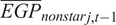
In column 2, we do a further decomposition of ΔEGP Differencet−1 and replace it with $ {{\overline{EGP}}_{star}}_{j,t-1} $
,
$ {{\overline{EGP}}_{star}}_{j,t-1} $
, $ {{\overline{EGP}}_{star}}_{j,t-2} $
,
$ {{\overline{EGP}}_{star}}_{j,t-2} $
, $ {{\overline{EGP}}_{nonstar}}_{j,t-1} $
,
$ {{\overline{EGP}}_{nonstar}}_{j,t-1} $
,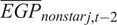 $ {{\overline{EGP}}_{nonstar}}_{j,t-2} $
as separate variables. The coefficients again make intuitive sense. The coefficient on
$ {{\overline{EGP}}_{nonstar}}_{j,t-2} $
as separate variables. The coefficients again make intuitive sense. The coefficient on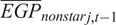 $ {{\overline{EGP}}_{nonstar}}_{j,t-1} $
is the most economically and statistically significant variable with coefficient value 0.49 and t-value 8.4. This is not surprising because it is also the lagged dependent variable.
$ {{\overline{EGP}}_{nonstar}}_{j,t-1} $
is the most economically and statistically significant variable with coefficient value 0.49 and t-value 8.4. This is not surprising because it is also the lagged dependent variable.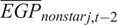 $ {{\overline{EGP}}_{nonstar}}_{j,t-2} $
is statistically insignificant (t-value 1.3) and close to 0 with coefficient value 0.04. The star firm coefficients
$ {{\overline{EGP}}_{nonstar}}_{j,t-2} $
is statistically insignificant (t-value 1.3) and close to 0 with coefficient value 0.04. The star firm coefficients $ {{\overline{EGP}}_{star}}_{j,t-1} $
and
$ {{\overline{EGP}}_{star}}_{j,t-1} $
and $ {{\overline{EGP}}_{star}}_{j,t-2} $
are both statistically significant with coefficient values 0.229 (t-value 4.9) and − 0.139 (t-value −2.7), respectively. The results are consistent with our previous findings because the value of ΔEGP Differencet−1 increases with the first lag of stars’ earnings growth and decreases with the second lag of stars’ earnings growth.
$ {{\overline{EGP}}_{star}}_{j,t-2} $
are both statistically significant with coefficient values 0.229 (t-value 4.9) and − 0.139 (t-value −2.7), respectively. The results are consistent with our previous findings because the value of ΔEGP Differencet−1 increases with the first lag of stars’ earnings growth and decreases with the second lag of stars’ earnings growth.
Finally, one potential concern with our regression coefficient estimates is that they may suffer from a dynamic panel bias (Nickell (Reference Nickell1981)) because the lagged dependent variable is included as a control variable. We address this issue in detail in Section A of the Supplementary Material where we first discuss the magnitude of the potential bias and show that it is insignificant in our setting. Nickell (Reference Nickell1981) shows that the bias is inversely proportional to the number of time periods in the panel, and our quarterly panel has sufficient length to make the potential bias virtually nonexistent. For further robustness, in Table IA.8 in the Supplementary Material, we re-estimate the baseline regression using a two-step Arellano-Bond Generalized Method of Moments estimation procedure following Wintoki, Linck, and Netter (Reference Wintoki, Linck and Netter2012). This approach is immune to dynamic panel bias and produces results that are consistent with the findings in Table 3.
C. Which Components of Earnings Growth Does ΔEGP Difference Predict?
To better understand the nature of the spillover effect, we analyze which components of year-over-year operating income growth are most sensitive to variation in ΔEGP Differencet−1. Specifically, we analyze the extent to which the earnings growth spillover effect can be attributed to changes in sales volume, operating profit margin, and its underlying subcomponents. An analysis on earnings growth subcomponents requires data from Compustat, and this analysis builds on the previous operating income/assets analysis in Table IA.6 in the Supplementary Material.
In our decomposition, we first divide total operating income before depreciation (OIBDP) for each firm i and quarter t into two subparts: one capturing OIBDP growth due to changes in sales volume and another capturing the effect of changes in operating expense-to-sales ratio. OIBDP is based on Compustat item OIBDPQ, which is defined as revenue (SALE) measured using item SALEQ minus total operating expenses (OPEX) measured using item XOPRQ:
 $$ OIBDP= SALE- OPEX= SALE\times \left(1-\frac{OPEX}{SALE}\right) $$
We use this identity as the basis for our decomposition, splitting the year-over-year change in operating income into two components that capture the effect of the change in SALE and OPEX/SALE while keeping the other variable fixed. The first component, $ \Delta {OIBDP_{Volume}}_{i,t} $
, measures the portion of the change driven by changes in SALE while holding the previous year’s OPEX/SALE ratio constant. It captures the OIBDP change attributable to sales volume growth under the assumption that sales volume is proportional to OPEX. The second component,
$ \Delta {OIBDP_{Volume}}_{i,t} $
, measures the portion of the change driven by changes in SALE while holding the previous year’s OPEX/SALE ratio constant. It captures the OIBDP change attributable to sales volume growth under the assumption that sales volume is proportional to OPEX. The second component, $ \Delta {OIBDP_{Margin}}_{i,t} $
, captures the effect of changes in the OPEX/SALE ratio itself, reflecting how shifts in operating efficiency or cost structure contribute to the overall change in operating income. By construction, these two components sum to the total change in operating income and the specific formulas are as follows:
$ \Delta {OIBDP_{Margin}}_{i,t} $
, captures the effect of changes in the OPEX/SALE ratio itself, reflecting how shifts in operating efficiency or cost structure contribute to the overall change in operating income. By construction, these two components sum to the total change in operating income and the specific formulas are as follows:
 $$ \Delta {OIBDP_{Volume}}_{i,t}=\left[{SALE}_{i,t}-{SALE}_{i,t-4}\right]\times \left(1-\frac{OPEX_{i,t-4}}{SALE_{i,t-4}}\right), $$
 $$ \Delta {OIBDP_{Margin}}_{i,t}={SALE}_{i,t}\times \left[\left(1-\frac{OPEX_{i,t}}{SALE_{i,t}}\right)-\left(1-\frac{OPEX_{i,t-4}}{SALE_{i,t-4}}\right)\right]. $$
To ensure appropriate comparisons across firms, we scale all variables by total assets from the previous fiscal year (Compustat item AT).Footnote 18
We further break down ΔOIBDPMargin into two subcomponents, which capture the effect of profit margin change relative to cost of goods sold and relative to other operational factors. Cost of goods sold is defined as Compustat item COGSQ, and it represents a major component of OPEX. The key insight is that the OPEX/SALE ratio can be expressed as the product of OPEX/COGS and COGS/SALE. Accordingly, we decompose ΔOIBDPMargin to separately capture the impact of changes in the share of COGS relative to sales and changes in OPEX relative to COGS, which reflect other operational efficiencies.
This decomposition connects to OIBDP through the following identity:
 $$ OIBDP= SALE\times \left(1-\frac{COGS}{SALE}\times \frac{OPEX}{COGS}\right). $$
The subcomponents are
 $$ \Delta {OIBDP_{Margin\;\left(\frac{COGS}{SALE}\right)}}_{i,t}={SALE}_{i,t}\times \left[\left(1-\frac{COGS_{i,t}}{SALE_{i,t}}\right)-\left(1-\frac{COGS_{i,t-4}}{SALE_{i,t-4}}\right)\right]\times \frac{OPEX_{i,t}}{COGS_{i,t}}, $$
 $$ \Delta {OIBDP_{Margin\left(\frac{COGS}{OPEX}\right)}}_{i,t}={\displaystyle \begin{array}{l}{SALE}_{i,t}\times \left[\left(1-\frac{OPEX_{i,t}}{COGS_{i,t}}\right)-\left(1-\frac{OPEX_{i,t-4}}{COGS_{i,t-4}}\right)\right]\\ {}\times \frac{COGS_{i,t-4}}{SALE_{i,t-4}}.\end{array}} $$
These subcomponents sum up to $ \Delta {OIBDP_{Margin}}_{i,t} $
in equation (5).Footnote
19 The first subcomponent measures the OIBDP change that is attributable to profit margin relative to COGS and the second component captures any residual change in the ΔOIBDPMargin component.
$ \Delta {OIBDP_{Margin}}_{i,t} $
in equation (5).Footnote
19 The first subcomponent measures the OIBDP change that is attributable to profit margin relative to COGS and the second component captures any residual change in the ΔOIBDPMargin component.
Table 4 reports results from industry-level regressions that use ΔEGP Differencej, t−1 to explain the average value of each of the earnings components and subcomponents among nonstar firms. These regressions are otherwise identical to our baseline earnings growth specification in column 3 of Table 3. To make it easier to compare the magnitude of ΔEGP Difference coefficients across different specifications, we standardize the dependent and independent variables.
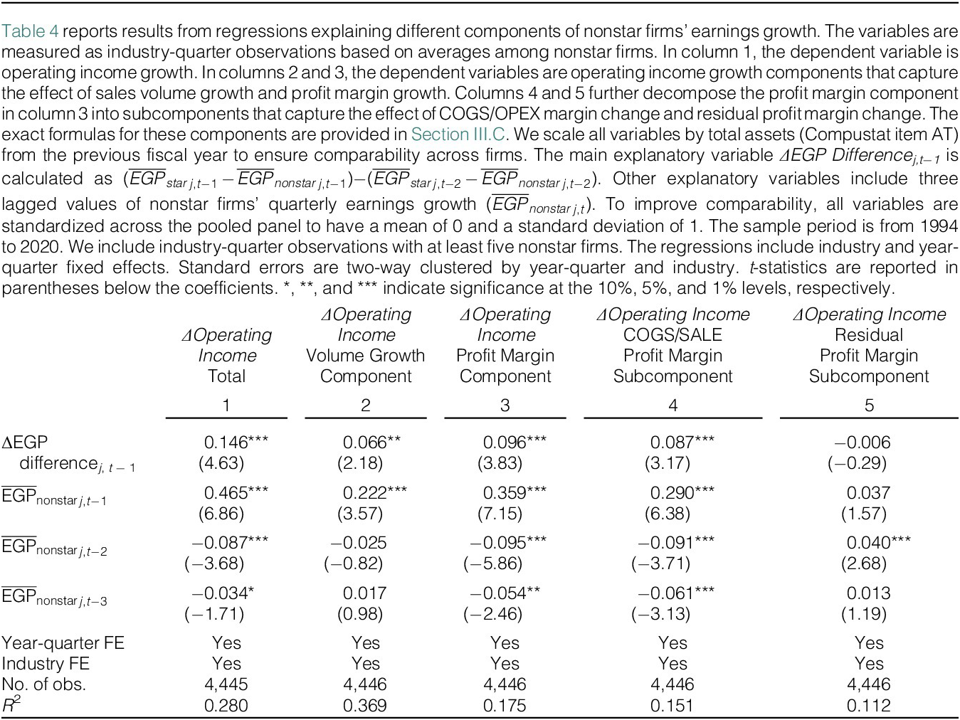
Column 1 first verifies that ΔEGP Difference can predict OIBDP growth in addition to earnings growth. The earnings growth coefficient is 0.146 with t-value of 4.63, indicating that a 1-standard-deviation increase in ΔEGP Difference is associated with a 0.15-standard-deviation increase in OIBDP growth. When we decompose total OIBDP growth into ΔOIBDPVolume and ΔOIBDPMargin in columns 2 and 3, we find that ΔEGP Difference can statistically significantly predict changes in both components, but the profit margin component is more responsive to changes in ΔEGP Difference. The coefficient on the profit margin component is 45% higher than the coefficient on the volume component (0.096 vs. 0.066). The t-values of the two components are 3.83 and 2.18, respectively.
The additional decomposition into profit margin subcomponents in columns 4 and 5 reveals that the profit margin effect is based on changes in profit relative to cost of goods sold rather than on other operational efficiencies. ΔEGP Difference can statistically significantly predict changes in the COGS/SALE subcomponent with coefficient values 0.087 and t-value of 3.17, whereas the coefficient on the COGS/OPEX subcomponent is statistically insignificant with coefficient value −0.006 and t-value of −0.29. Altogether, the OIBDP decomposition results indicate that the earnings growth changes predicted by ΔEGP Difference are related to changes in profit margins and sales volume, and the profit margin component is more sensitive to ΔEGP Difference. The impact on the profit margin component is related to markup relative to cost of goods sold rather than other operational efficiencies.Footnote 20
D. Predicting Job Postings
So far, our results show that star firms’ relative earnings performance predicts nonstar firms’ earnings growth. We next test whether ΔEGP Difference also predicts nonstar firms’ job postings—a timely indicator of firm growth and labor demand. Shifts in star firms’ performance may affect nonstar hiring through profitability spillovers and local multiplier effects (Moretti, Reference Moretti2010).
To test this conjecture, we estimate quarterly industry-level panel regressions where we explain the relative change in the average number of job postings for nonstar and star firms with ΔEGP Difference. Specifically, the dependent variable is defined as $ \left({{\overline{JP}}_{star/ nonstar}}_{j,t}-{{\overline{JP}}_{star/ nonstar}}_{j,t-1}\right)/{{\overline{JP}}_{star/ nonstar}}_{j,t-1} $
, where
$ \left({{\overline{JP}}_{star/ nonstar}}_{j,t}-{{\overline{JP}}_{star/ nonstar}}_{j,t-1}\right)/{{\overline{JP}}_{star/ nonstar}}_{j,t-1} $
, where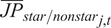 $ {{\overline{JP}}_{star/ nonstar}}_{j,t} $
is the average number of job postings by star/nonstar firms in industry j in quarter t. Like our previous earnings regressions, these regressions control for lagged values of earnings growth, and they include year-quarter fixed effects and industry fixed effects. We also estimate specifications where we control for the lagged value of average job postings.
$ {{\overline{JP}}_{star/ nonstar}}_{j,t} $
is the average number of job postings by star/nonstar firms in industry j in quarter t. Like our previous earnings regressions, these regressions control for lagged values of earnings growth, and they include year-quarter fixed effects and industry fixed effects. We also estimate specifications where we control for the lagged value of average job postings.
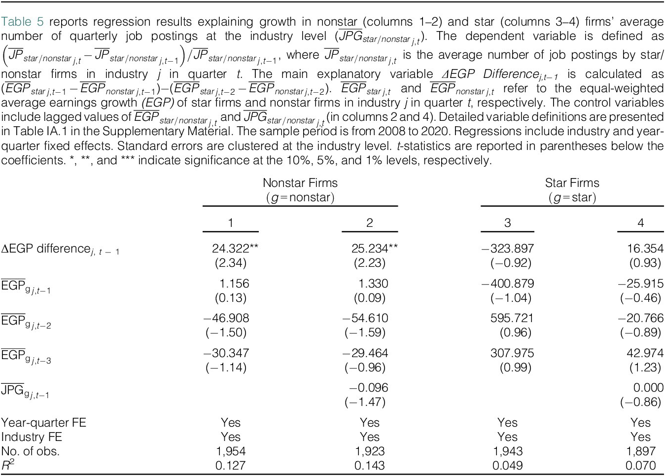
Table 5 shows that lagged ΔEGP Difference statistically significantly predicts nonstar firms’ job postings. The coefficient ranges from 24.32 (t-stat = 2.33) to 25.32 (t-stat = 2.22), implying a 1-standard-deviation increase in ΔEGP Difference raises nonstar job postings by 34%–36%. In contrast, the effect on star firms’ own postings is negative and insignificant. This is consistent with the hypothesis that star firms’ relative performance predicts nonstar firms’ hiring but not their own.
E. Predicting Industry-Level GDP and Employment Growth with ΔEGP Difference
Building on the predictability in earnings growth and job postings, we hypothesize that ΔEGP Difference also contains information relevant for predicting broader industry-level economic fundamentals. We study its ability to predict quarterly real GDP and employment growth. These analyses differ from the previous regressions because industry aggregates include listed and unlisted firms, and we cannot isolate star and nonstar effects separately. Also, the GDP time series starts in 2006 due to data limitations.
Table 6 reports regressions of quarterly year-over-year industry GDP growth (Panel A) and employment growth (Panel B) on lagged ΔEGP Difference, with controls for past industry earnings growth and lagged GDP or employment growth. In Panel A, ΔEGP Difference is positively and statistically significantly related to future industry GDP growth, with coefficients from 0.345 to 0.442 (significant at the 10% level or higher). Economically, a 1-standard-deviation increase predicts a 0.5–0.6 percentage point rise in GDP growth. This response is comparatively higher than the effect of a 1-standard-deviation change on future earnings growth in the regressions of Table 3.
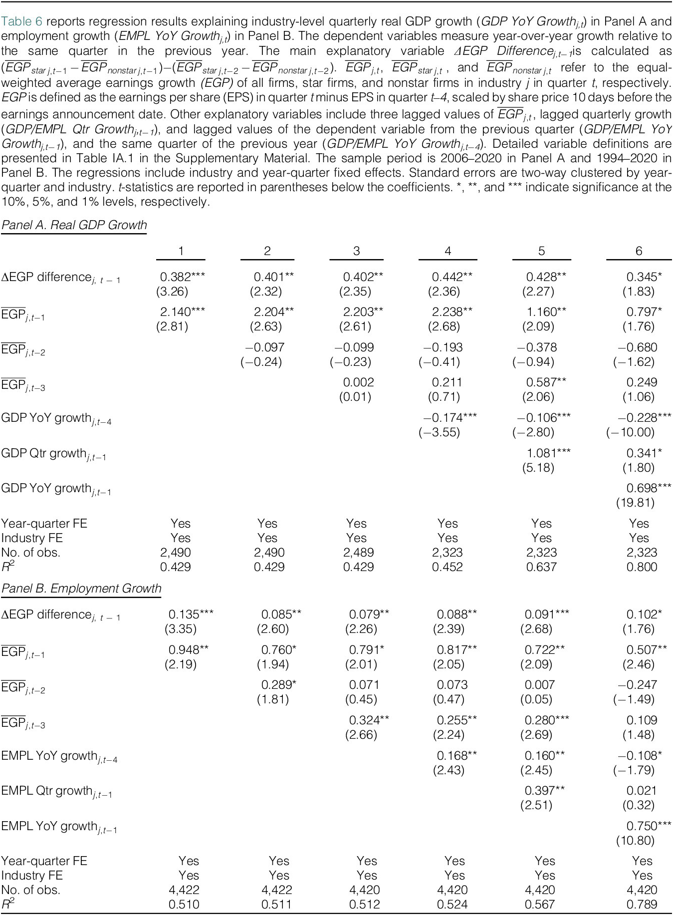
Panel B shows a similar positive link for employment: higher relative star firm earnings growth predicts higher industry employment growth next quarter. The coefficients (0.079–0.135) imply a 0.1–0.2 percentage point increase in employment growth per standard deviation increase in ΔEGP Difference. The results are statistically significant at the 10% level or higher. Together, these findings indicate that star firms’ relative performance predicts not only nonstar firm outcomes but also broader industry-level growth and labor market trends.
F. Predicting Industry-Level GDP with the Change in Star Firms’ P/E Ratios
We also examine stars’ ability to predict GDP growth using an alternative measure based on growth expectations embedded in firm valuations. Previously, Bekaert et al. (Reference Bekaert, Harvey, Lundblad and Siegel2007) measure a country’s growth opportunities using a price-to-earnings (P/E) ratio based on its industry mix valued at global P/E ratios. They find that the country-specific P/E ratio can predict future GDP growth and investment, which indicates that aggregate P/E ratios contain information that is relevant for predicting future economic growth.
Building on this idea, we test whether changes in star firms’ P/E ratios signal broader industry growth opportunities. If star firms’ growth spills over to other firms, then stars’ P/E ratios may better capture industry-level growth expectations than nonstars’ P/E ratios, especially if markets underreact to these spillovers.
P/E ratios reflect long-term growth opportunities, and we test the hypothesis by estimating regressions where we explain change in annual GDP growth at the industry level (ΔGDP Ann Growthj,t) with the change in star firms’ and nonstar firms’ P/E ratio. Specifically, we define $ P/E\;{Growth_{star/ nonstar}}_{j,t-1} $
as (
$ P/E\;{Growth_{star/ nonstar}}_{j,t-1} $
as ( $ P/{E_{star/ nonstar}}_{j,t-1}-P/{E_{star/ nonstar}}_{j,t-2} $
)
$ P/{E_{star/ nonstar}}_{j,t-1}-P/{E_{star/ nonstar}}_{j,t-2} $
) $ /P/{E_{star/ nonstar}}_{j,t-2} $
. The variable
$ /P/{E_{star/ nonstar}}_{j,t-2} $
. The variable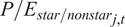 $ P/{E_{star/ nonstar}}_{j,t} $
refers to industry j’s sum of star/nonstar firms’ market capitalization in December of fiscal year t divided by their sum of earnings before extraordinary items (Compustat item EPSPX times shares outstanding, item CSHO) for fiscal year t. Regressions include industry fixed effects and lagged P/E growth and are estimated both with and without time fixed effects.
$ P/{E_{star/ nonstar}}_{j,t} $
refers to industry j’s sum of star/nonstar firms’ market capitalization in December of fiscal year t divided by their sum of earnings before extraordinary items (Compustat item EPSPX times shares outstanding, item CSHO) for fiscal year t. Regressions include industry fixed effects and lagged P/E growth and are estimated both with and without time fixed effects.
The results in Table 7 show that star firms’ relative P/E changes statistically significantly predict industry GDP growth changes, whereas nonstars’ P/E changes do not. The coefficient on $ P/E\;{Growth_{star}}_{j,t-1} $
is 0.010 with t-value of 2.57 when time fixed effects are included and 0.012 with t-value of 2.18 without the time fixed effects. In contrast, the corresponding nonstar coefficients are statistically insignificant with coefficient value 0.005 and t-values of 1.35 and 1.20, respectively. Columns 3 and 6 include both the star and nonstar variables as separate predictors in regressions estimated with and without time fixed effects. In both cases, the coefficient value on
$ P/E\;{Growth_{star}}_{j,t-1} $
is 0.010 with t-value of 2.57 when time fixed effects are included and 0.012 with t-value of 2.18 without the time fixed effects. In contrast, the corresponding nonstar coefficients are statistically insignificant with coefficient value 0.005 and t-values of 1.35 and 1.20, respectively. Columns 3 and 6 include both the star and nonstar variables as separate predictors in regressions estimated with and without time fixed effects. In both cases, the coefficient value on $ P/E\;{Growth_{star}}_{j,t-1} $
remains almost unchanged and statistically significant, whereas the
$ P/E\;{Growth_{star}}_{j,t-1} $
remains almost unchanged and statistically significant, whereas the $ P/E\;{Growth_{nonstar}}_{j,t-1} $
coefficients are statistically insignificant. In economic terms, a 1-standard-deviation change in
$ P/E\;{Growth_{nonstar}}_{j,t-1} $
coefficients are statistically insignificant. In economic terms, a 1-standard-deviation change in $ P/E\;{Growth_{star}}_{j,t-1} $
predicts a 0.8 percentage point increase in the change in annual GDP growth. This effect corresponds to 9.3% of the standard deviation of changes in annual industry GDP growth.
$ P/E\;{Growth_{star}}_{j,t-1} $
predicts a 0.8 percentage point increase in the change in annual GDP growth. This effect corresponds to 9.3% of the standard deviation of changes in annual industry GDP growth.

These results reinforce our earlier findings: star firms provide predictive signals about broader economic outcomes, not just about firm-specific performance. Together, the GDP and employment results highlight the wider economic importance of star firms’ information spillovers. The findings also show that star firms’ predictive ability extends to performance in nonfinancial outcomes.
IV. Economic Channels Behind the Industry Spillover Effect
In this section, we analyze the economic channels and industry dynamics that can contribute to the earnings growth spillover effect documented in Section III. We first describe the potential mechanisms through which star firms’ information predicts nonstar firms’ earnings and then assess the empirical support for each channel.
A. Potential Economic Channels Behind the Spillover Effect
Stars as price setters and price markup spillover. Previous literature provides evidence that the largest firms in the economy have higher price markups (Autor et al. (Reference Autor, Dorn, Katz, Patterson and Van Reenen2020), De Loecker et al. (Reference De Loecker, Eeckhout and Unger2020)), suggesting market power is central to star firms’ dominance. If star firms have greater pricing power, they may act as price setters within industries, while nonstar firms adjust their prices accordingly. When star firms raise or lower prices, nonstars’ profits would change in tandem as they follow the stars’ pricing decisions.
Technology spillover related to product market innovation. Product market innovation spillovers where new products, services, or technologies developed by star firms are adopted by nonstar firms can potentially result in earnings spillovers. Improved products can result in higher sales volume, as well as higher price markups. Easier access to human capital (Choi et al. (Reference Choi, Lou and Mukherjee2026)) and better management quality can contribute to stars’ innovativeness.Footnote 21
Technology spillover related to productivity innovation. Technology spillovers can also stem from productivity innovations. If star firms develop cost-saving production techniques that nonstars can imitate, this may lower unit costs across the industry, resulting in earnings spillovers.
Supply chain and vertical integration effects. Positive shocks to star firms’ profitability can affect other firms that are connected to them through the supply chain or other intra-industry connections.
Schumpeterian competition with negative externalities on nonstar firms. Star firms’ innovations could trigger Schumpeterian competition, spurring creative destruction that reduces nonstar firms’ future earnings (Aghion and Howitt (Reference Aghion and Howitt1992), Cheng, Vyas, Wittenberg-Moerman, and Zhao (Reference Cheng, Vyas, Wittenberg-Moerman and Zhao2025)).
B. Empirical Evidence on Economic Channels
Our previous earnings growth decomposition results are consistent with the price markup channel where stars function as price setters. The finding that the COGS profit margin component is most responsive to changes in ΔEGP Difference is in line with this explanation because it captures price markup relative to unit costs. To further test the price markup spillover hypothesis, we analyze whether star firms’ price markup changes predict nonstars’ price markup changes using a detailed price markup definition introduced by De Loecker et al. (Reference De Loecker, Eeckhout and Unger2020). Their markup variable accounts for user cost of capital and complements Compustat with other data sources.Footnote 22 Because these data are annual, we conduct the analysis at the annual level.
In Table IA.10 in the Supplementary Material, we estimate regressions where we explain nonstars’ and stars’ average change in annual markup at the industry level with a variable labeled ΔMU Differencej, t − 1, which is defined similarly as ΔEGP Differencej, t − 1. It captures the difference between stars’ and nonstars’ average markup growth over the previous year. The regressions include year and firm fixed effects and control for three lagged values of markup growth. The results show that ΔMU Differencej, t − 1 can statistically significantly predict nonstars’ markup change with coefficient value 0.053 and t-value of 2.33, whereas the coefficient in the regression explaining stars’ markup growth is negative and statistically insignificant. These results provide further evidence that stars’ price markup changes lead nonstars’ price markup changes.Footnote 23
We also find evidence consistent with technology spillovers from star firms to nonstars but only related to product market innovation. To analyze the relevance of the technology spillover channel, we classify industries as high and low technology spillover industries using the Technology Spillover score developed by Bloom et al. (Reference Bloom, Schankerman and Van Reenen2013). Specifically, we calculate nonstar firms’ average Technology Spillover score with the same-industry stars within each industry-quarter. We then use the median industry scores to split industries into High Technology Spillover (above median) and Low Technology Spillover (below median) industries.
Panel A of Table 8 reports results from regressions explaining the main OIBDP growth subcomponents (ΔOperating IncomeVolume and ΔMargin) with ΔEGP Difference among High and Low Technology Spillover industries. We find that ΔEGP Difference coefficients in High Technology Spillover industries are higher for both the volume growth (0.121 vs. 0.054) and profit margin (0.172 vs. 0.048) components and the coefficients in the Low Technology Spillover industries are statistically insignificant.Footnote 24 These results provide evidence that ΔEGP Difference has a stronger ability to predict volume and profit margin changes in industries with high technological similarity. However, our evidence does not indicate that the technology spillovers are related to productivity innovation. Production can become more efficient either through the reduction of unit costs or through other operational efficiencies, but as discussed in Section III.C, we find no evidence that ΔEGP Difference predicts cost structure changes.
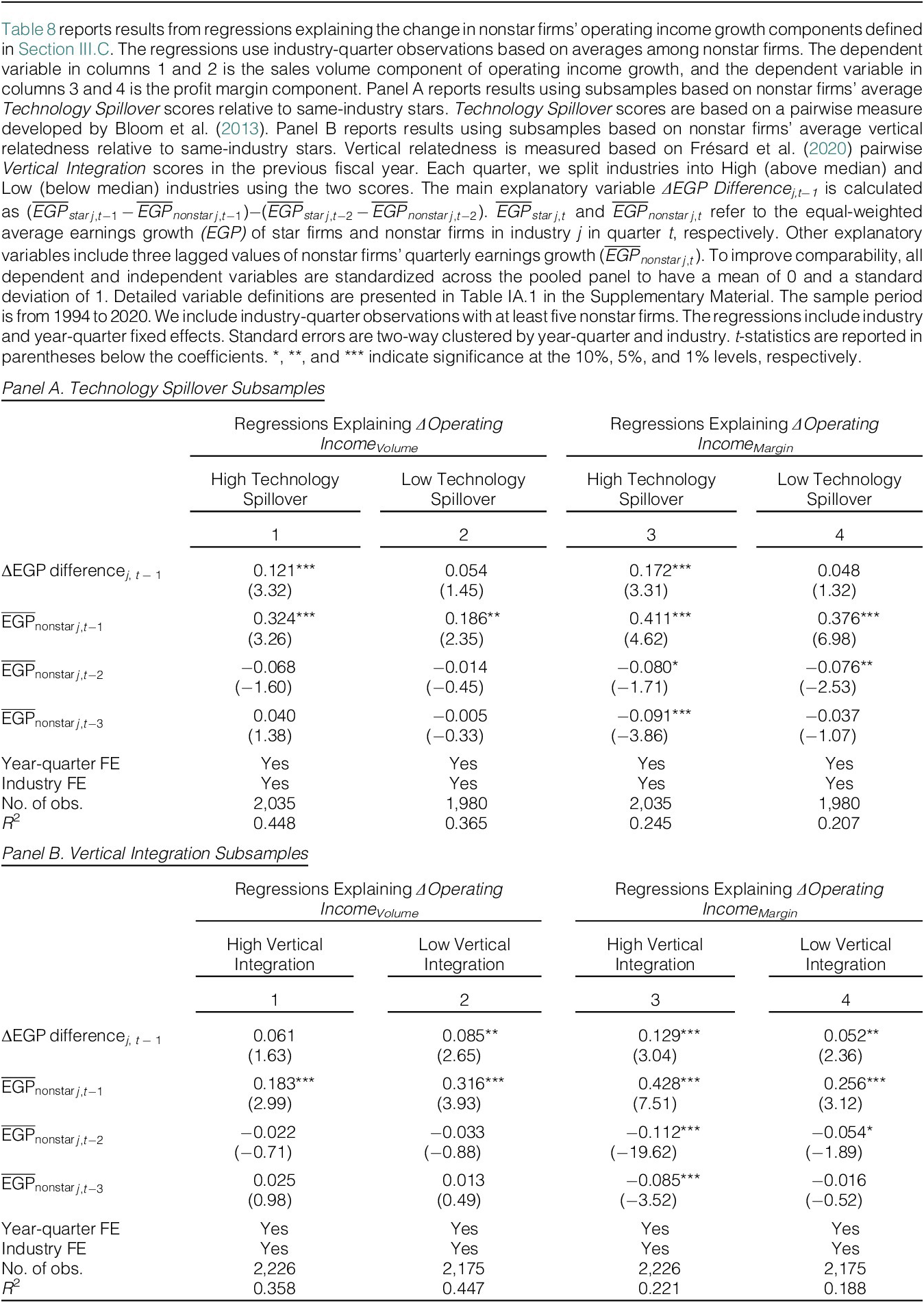
Next, we test the supply chain channel using Frésard et al.’s (Reference Frésard, Hoberg and Phillips2020) Vertical Integration scores to classify industries. Again, we split industries by median score and compare results (Table 8, Panel B).Footnote 25 We find that the ΔEGP Difference coefficient in regressions explaining ΔOIBDPMargin in High Vertical Integration industries (0.129 with t-value of 3.04) is higher than the corresponding coefficient in Low Vertical Integration industries (0.052 with t-value of 2.36). The coefficients on volume growth are close to each other (0.061 vs. 0.085), with only the Low Vertical Integration coefficient being statistically significant. These results suggest that profitability spillovers are larger in High Vertical Integration industries, and stars’ markup changes can potentially spread through the supply chain.
Our results are not consistent with the Schumpeterian competition channel where star firms’ innovation spurs creative destruction. Such effects may have an impact over a longer time period, but they are contrary to our findings because the ΔEGP Difference results suggest that positive earnings shocks to star firms predict positive future performance for nonstar firms.
Altogether, we find support for channels related to star firms as price setters, technology spillovers, and vertical integration effects. Any potential technology spillover effects seem to arise from product market innovation rather than from productivity innovation. Notably, all the spillover effects we find are positive, even in earnings growth subcomponents. While we cannot rule out that star firms’ dominance has negative effects on nonstar firms over the long run, in the short-term, star firms’ performance improvements predict positive earnings for nonstar firms in the future.
V. Star Firms and Earnings Surprises
Our earnings growth regression estimates indicate that star firms reflect information relevant to predicting nonstar firms’ future growth. A natural question to ask is whether market participants recognize this. In this section, we investigate whether sell-side analysts incorporate star firm earnings information when making forecasts on nonstar firms.
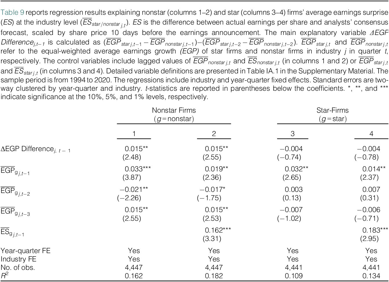
In the earnings surprise analysis, we use ΔEGP Differencej,t−1 to predict the average quarterly earnings surprise of either star or nonstar firms within industry j. Our regression specifications are similar to the earnings growth regressions reported in Table 3. We separately regress year-quarter earnings surprise average for industry-level star and nonstar firms on ΔEGP Differencej,t−1. We include lagged earnings surprises as control variables and include industry as well as year-quarter fixed effects.
In columns 1–3 of Table 9, we regress the average earnings surprise of nonstar firms (i.e., $ {{\overline{ES}}_{nonstar}}_{j,t} $
) on ΔEGP Differencej,t−1. We find that the ΔEGP Differencej,t−1 statistically significantly predicts the earnings surprise of nonstar firms. Specifically, the coefficient on ΔEGP Difference is positive and statistically significant with a coefficient value of 0.015 and t-statistic of 2.5. These results suggest that analysts underreact to the information reflected in star firms’ earnings growth. In economic terms, a 1-standard-deviation change in ΔEGP Difference corresponds to an increase in earnings surprise of nonstar firms that is 10% of the standard deviation of this measure.Footnote
26 In columns 4–6, we regress average consensus earnings surprise of star firms within the same industry (i.e.,
$ {{\overline{ES}}_{nonstar}}_{j,t} $
) on ΔEGP Differencej,t−1. We find that the ΔEGP Differencej,t−1 statistically significantly predicts the earnings surprise of nonstar firms. Specifically, the coefficient on ΔEGP Difference is positive and statistically significant with a coefficient value of 0.015 and t-statistic of 2.5. These results suggest that analysts underreact to the information reflected in star firms’ earnings growth. In economic terms, a 1-standard-deviation change in ΔEGP Difference corresponds to an increase in earnings surprise of nonstar firms that is 10% of the standard deviation of this measure.Footnote
26 In columns 4–6, we regress average consensus earnings surprise of star firms within the same industry (i.e., $ {{\overline{ES}}_{star}}_{j,t} $
) on ΔEGP Differencej,t−1. The coefficients on ΔEGP Difference are negative and insignificant and consistent with our previous earnings predictability results.
$ {{\overline{ES}}_{star}}_{j,t} $
) on ΔEGP Differencej,t−1. The coefficients on ΔEGP Difference are negative and insignificant and consistent with our previous earnings predictability results.
We also test whether star firms’ predictive ability extends beyond small firms. We classify the top 30% of firms based on market capitalization as large firms, the middle 40% as medium-sized firms, and the bottom 30% as small firms. Hou (Reference Hou2007) uses a similar categorization in a study on lead–lag effects in stock returns. Table IA.13 in the Supplementary Material repeats the earnings growth and earnings surprise predictability regressions of Tables 3 and 4 using two subsamples where we either exclude small nonstar firms or only include medium-sized nonstar firms. The ΔEGP Differencej,t−1 coefficients remain positive and statistically significant in these subsamples, indicating that star firms’ predictive ability is not limited to small firms. This evidence also differentiates our findings from previously documented lead–lag patterns in stock returns where large firms’ performance can exclusively predict the future performance of small firms (e.g., Lo and MacKinlay (Reference Lo and MacKinlay1990), Hou (Reference Hou2007)).
If analysts underreact to shifts in star firms’ relative earnings performance, markets may not fully incorporate this information into prices. As a result, star firms’ relative earnings could predict short-term returns of nonstar firms. To test this, we regress cumulative abnormal returns of nonstar firms around earnings announcements, aggregated at the industry level, on our key ΔEGP Differencej,t−1 measure. Some specifications add average earnings announcement returns of star and nonstar firms from the prior quarter as controls. All regressions include year-quarter and industry fixed effects, with standard errors clustered by year-quarter and industry.
Table 10 reports the market reaction regression results. We find that ΔEGP Differencej,t−1 positively predicts cumulative abnormal returns of nonstar firms in a [0, 2] window around earnings announcements. Specifically, as reported in column 1, one unit increase in ΔEGP Differencej,t−1 is associated with a 6.8% higher return for nonstar firms around earnings announcements. This effect is statistically significant at the 5% level. In columns 2 and 3, we control for lagged announcement returns for nonstar and star firms as additional control variables. Star firms’ earnings performance still predicts nonstar firms’ returns. As a placebo test, we estimate the same regression on star firm returns and do not find any significant effect (see columns 4–6).
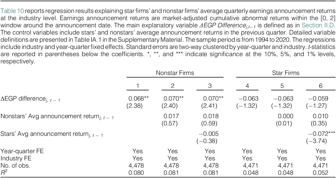
Together, these results indicate that star firms’ relative earnings performance positively predicts nonstar firms’ returns, suggesting that star firms reflect relevant information about nonstar firms that is not already incorporated into prices.
VI. Star Firms and Stock Returns
Our previous findings indicate that changes in star firms’ relative earnings performance can predict nonstars’ earnings announcement returns. To further explore the asset pricing implications, we develop a trading strategy that leverages cross-sectional differences in star firms’ performance shifts and examine potential lead–lag relationships between same-industry stars’ and nonstars’ returns.
A. Earnings Performance Shifts and Stock Returns
We start by creating market value-weighted quintile portfolios of nonstar firms with CRSP share codes 10 or 11 in industries with the highest and lowest lagged values of ΔEGP Difference. Each month, we form quintiles by sorting all industries using the $ \varDelta $
EGP difference measured at the end of the previous month (i.e., ΔEGP Difference Monthlyj,t−1). ΔEGP Difference Monthly is calculated using earnings announcements from months t−1 to t−3.
$ \varDelta $
EGP difference measured at the end of the previous month (i.e., ΔEGP Difference Monthlyj,t−1). ΔEGP Difference Monthly is calculated using earnings announcements from months t−1 to t−3.
We construct a value-weighted long portfolio that invests in nonstar portfolios from the 11 highest-ranked industries and a value-weighted short portfolio that invests in nonstar portfolios from the 11 lowest-ranked industries. These portfolios correspond to the top and bottom quintile within the 55 industries for which we have sufficient observations. Within each value-weighted quintile, an industry’s nonstar portfolio weight is based on the sum of the market capitalizations of all nonstar firms in that industry at the end of the previous month. We then define a long–short portfolio strategy that takes a long position in the quintile of industries with the highest lagged ΔEGP Difference Monthly values and takes a short position in industries with the lowest ΔEGP Difference Monthly values. The mean return of the lowest and highest quintile portfolios are 0.698% and 1.292% (see Table IA.14 in the Supplementary Material), respectively.
We compute the monthly value-weighted returns of each quintile as well as the Q5−Q1 long–short portfolio and regress the excess portfolio returns on the Fama and French (Reference Fama and French2015) five factors plus the momentum factor. Table 11 reports the portfolio alphas and factor beta estimates. The beta estimates indicate that Q5 firms, which are in industries with larger positive star firm earnings performance shifts, are typically profitable firms. In contrast, firms facing low or negative shifts in peer star firms’ earnings, included in Q1 portfolios, are typically value stocks. Both extreme quintiles have positive loadings on size and negative loadings on momentum.
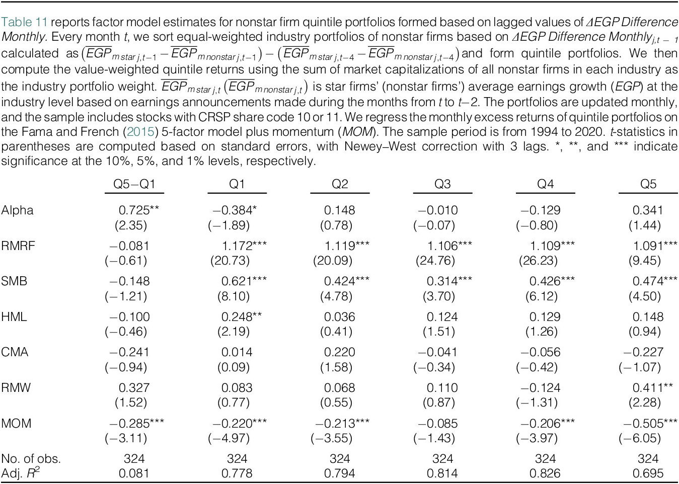
The Q1 and Q5 portfolios generate monthly alphas of −0.384% and 0.341%, respectively. The other quintile portfolios do not produce significant alphas, suggesting that almost all of the return predictability comes from firms with extreme star firm earnings performance shifts. The long–short portfolio results based on Q5−Q1 indicate that high ΔEGP Difference Monthly firms outperform the low ΔEGP Difference Monthly firms by 0.725% per month (t-stat = 2.35) on a risk-adjusted basis.
B. Lead–Lag Relation in Stock Returns
So far, our results indicate that star firms’ relative earnings growth acceleration predicts the earnings growth of nonstar firms, and this information is not fully incorporated in stock prices. We now directly examine the relation between the returns of star and nonstar firms. Based on the findings in the comovement literature (e.g., Hou (Reference Hou2007), Hameed, Morck, Shen, and Yeung (Reference Hameed, Morck, Shen and Yeung2015)), we posit that underreaction related to information spillover between connected firms may generate a predictable lead–lag relation in stock returns.
To test the lead–lag relation between star and nonstar returns, each month, we sort nonstar firms by the value-weighted average return of same-industry star firms in the previous month. We then calculate the value-weighted average monthly returns of the quintile portfolios and adjust for risk using the 6-factor model described in the previous subsection.
Table 12, Panel A reports the portfolio abnormal returns and the factor betas. The average monthly abnormal return spread between the top and bottom quintile portfolios (Q5−Q1) is 0.465% (t-stat = 2.41), suggesting that nonstar firms in industries with the best lagged star firm performance outperform those in industries with the worst lagged star performance by 47 basis points per month. The regression alphas show a significant lead–lag relation between the returns of stars and nonstars, particularly in industries with extremely high (Q5) and low (Q1) past star firm returns. Specifically, Q5 and Q1 quintiles generate monthly alphas of 0.239% (t-stat = 2.02) and −0.226% (t-stat = −1.77), respectively.

In Panel B, we do a placebo test to check whether nonstar firms’ returns predict star firms’ returns. In this case, we form star firm quintiles by sorting on lagged value-weighted nonstar firms’ returns. We find an insignificant long–short portfolio alpha, suggesting that nonstar firms’ returns do not contain useful information about future performance of star firms. This one-way lead–lag return comovement between star and nonstar firms is in line with our earlier finding that only star firms’ earnings performance changes contain relevant information about nonstar firms’ future performance.
VII. Is the Star Firm Effect Merely a Large Firm Effect?
In the last set of tests, we examine whether other large firms exhibit the same ability to predict the outcomes of other firms as star firms. We repeat our main analyses using an alternative specification where we assign the next four largest firms in each industry as “star substitutes.” This means that we effectively replace the stars with the same number of other large firms. As before, the regressions include industry-quarter observations with at least five nonstar firms.
Table IA.15 in the Supplementary Material reports results from regressions where we explain nonstar firms’ earnings growth, earnings surprises, and earnings announcement returns with ΔEGP Differencej,t−1 calculated using these star substitutes and Table IA.16 in the Supplementary Material reports 6-factor alphas from nonstar firm portfolios formed based on the corresponding ΔEGP Difference Monthlyj,t−1. The regressions in these tables in the Supplementary Material are identical to the specifications in Tables 3 and 9–11. The substitute ΔEGP Differencej,t−1 is based on the relative earnings growth difference between the substitute star firms and the remaining nonstar firms.
Panel A of Table IA.15 in the Supplementary Material shows that star substitutes can predict nonstars’ earnings growth, but the coefficient magnitudes are 40%–60% of the corresponding coefficients for actual stars. However, the substitute stars do not have predictive ability in any of the analyses that involve analyst forecasts or stock returns. The substitute star ΔEGP Differencej,t−1 coefficients are statistically insignificant in regressions explaining nonstar firms’ earnings surprises (Table IA.15, Panel B in the Supplementary Material) and earnings announcement returns (Table IA.15, Panel C in the Supplementary Material), and the long–short alpha in the portfolio test based on ΔEGP Difference Monthlyj,t−1 is also statistically insignificant (Table IA.16 in the Supplementary Material). Together, these placebo tests confirm that the effects we identify are specific to star firms and are not merely general large-firm effects.
VIII. Summary and Conclusions
This study examines whether information from very large and dominant “star” firms can predict the future performance of other connected firms and the broader industry around them. Star firms are known to have a large and sometimes disproportionate impact on various macroeconomic outcomes, and they can affect other firms through various spillover and multiplier effects. Our key conjecture is that changes in star firms’ earnings performance predict the future earnings and growth of other related firms. Further, market participants, such as sell-side equity analysts, may not fully incorporate information from star firms into their earnings forecasts of related firms. Consequently, financial information of industry star firms would predict patterns in firm-level earnings and returns of nonstar firms.
We test these conjectures using the definition of industry star firms developed in Gutiérrez and Philippon (Reference Gutiérrez and Philippon2019). Consistent with our conjectures, we find that changes in star firms’ relative earnings performance contain incremental information, as they predict the earnings growth, earnings surprises, and labor market activities (i.e., job postings) of other nonstar firms in the same industry. At the industry level, star firms’ earnings performance shifts serve as a leading indicator that can predict future GDP and employment growth. We find that spillover effects related to price markups, technology, and vertical integration are potential economic channels behind these patterns.
Notably, these predictive signals are not fully reflected in stock prices: a long–short trading strategy based on changes in star firms’ relative earnings achieves an annualized risk-adjusted return exceeding 8%. Overall, these findings provide market- and operating-performance-based evidence of the economic importance of star firms and highlight the broader role of very large firms in financial markets.
Supplementary Material
To view supplementary material for this article, please visit http://doi.org/10.1017/S0022109026102610.



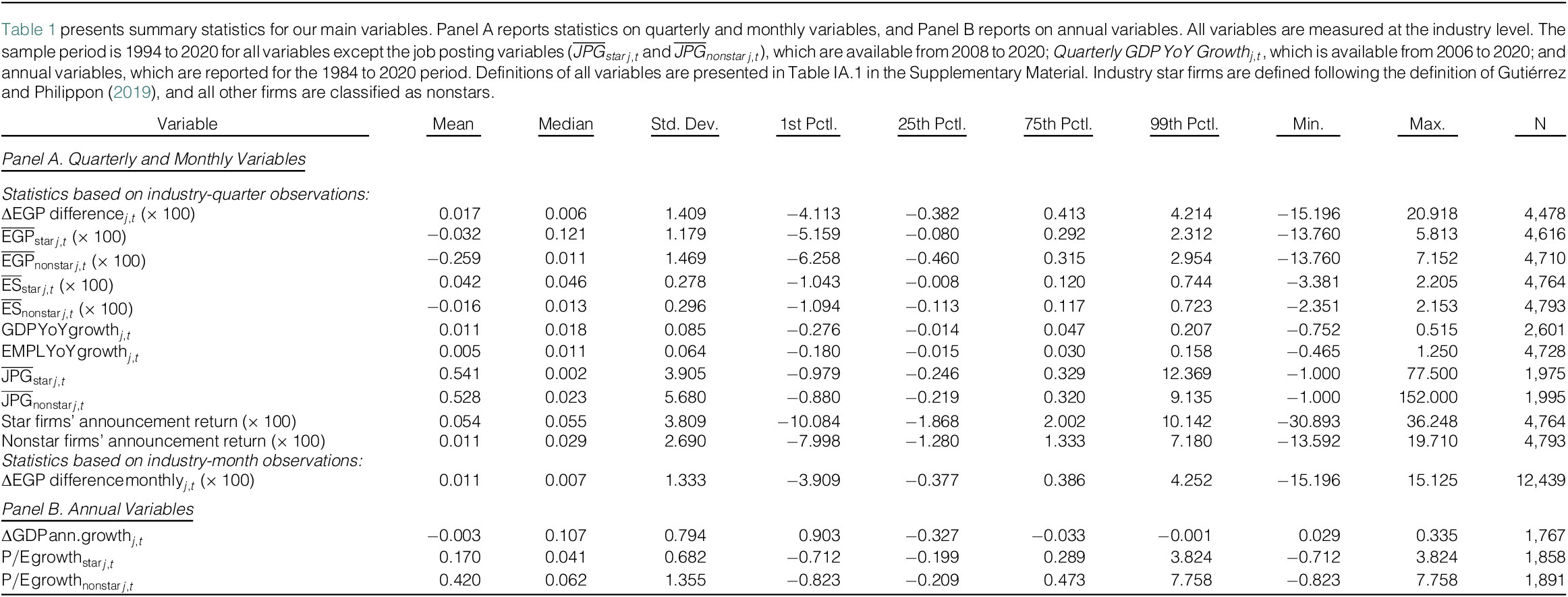
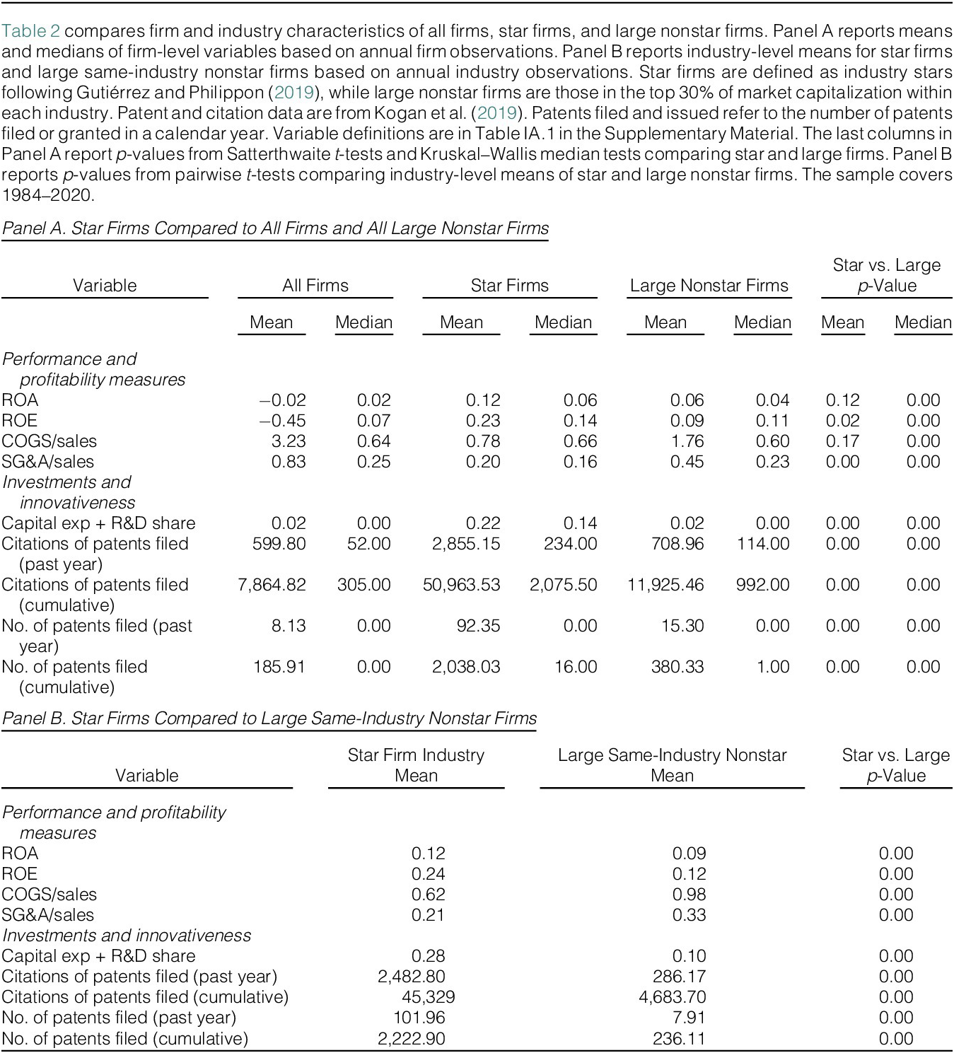
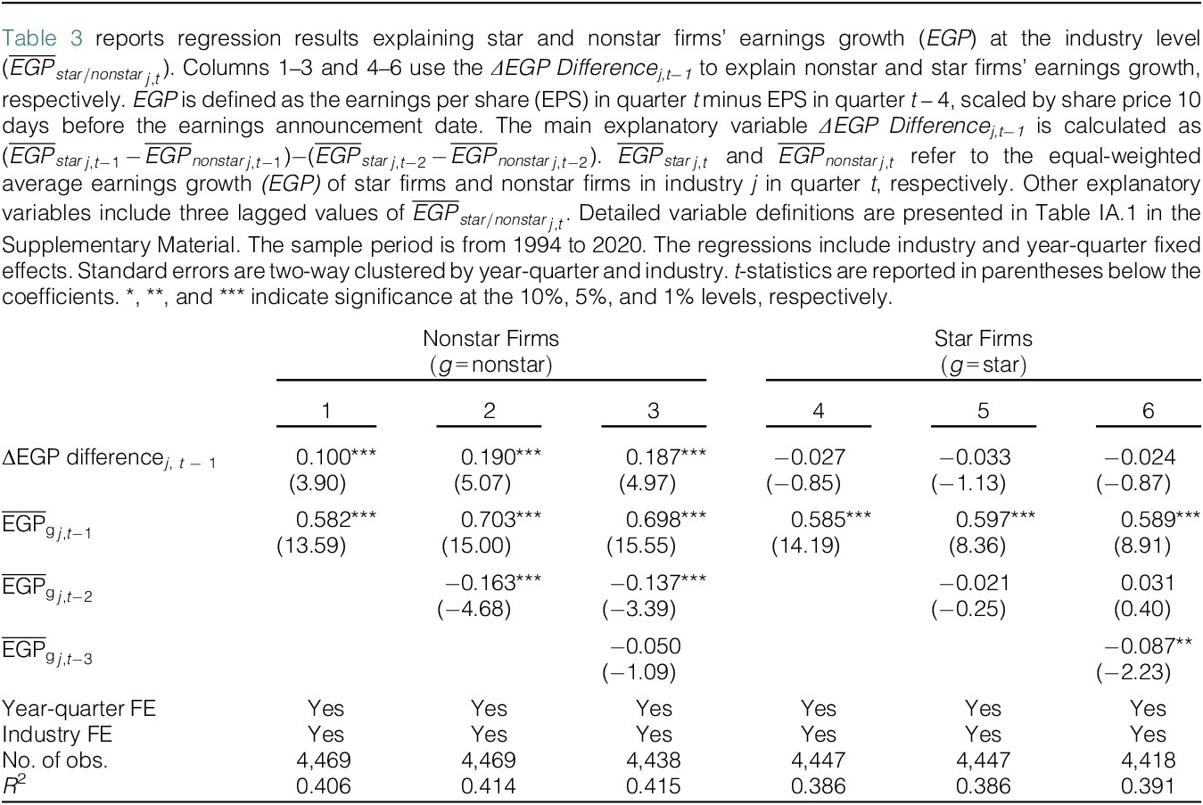
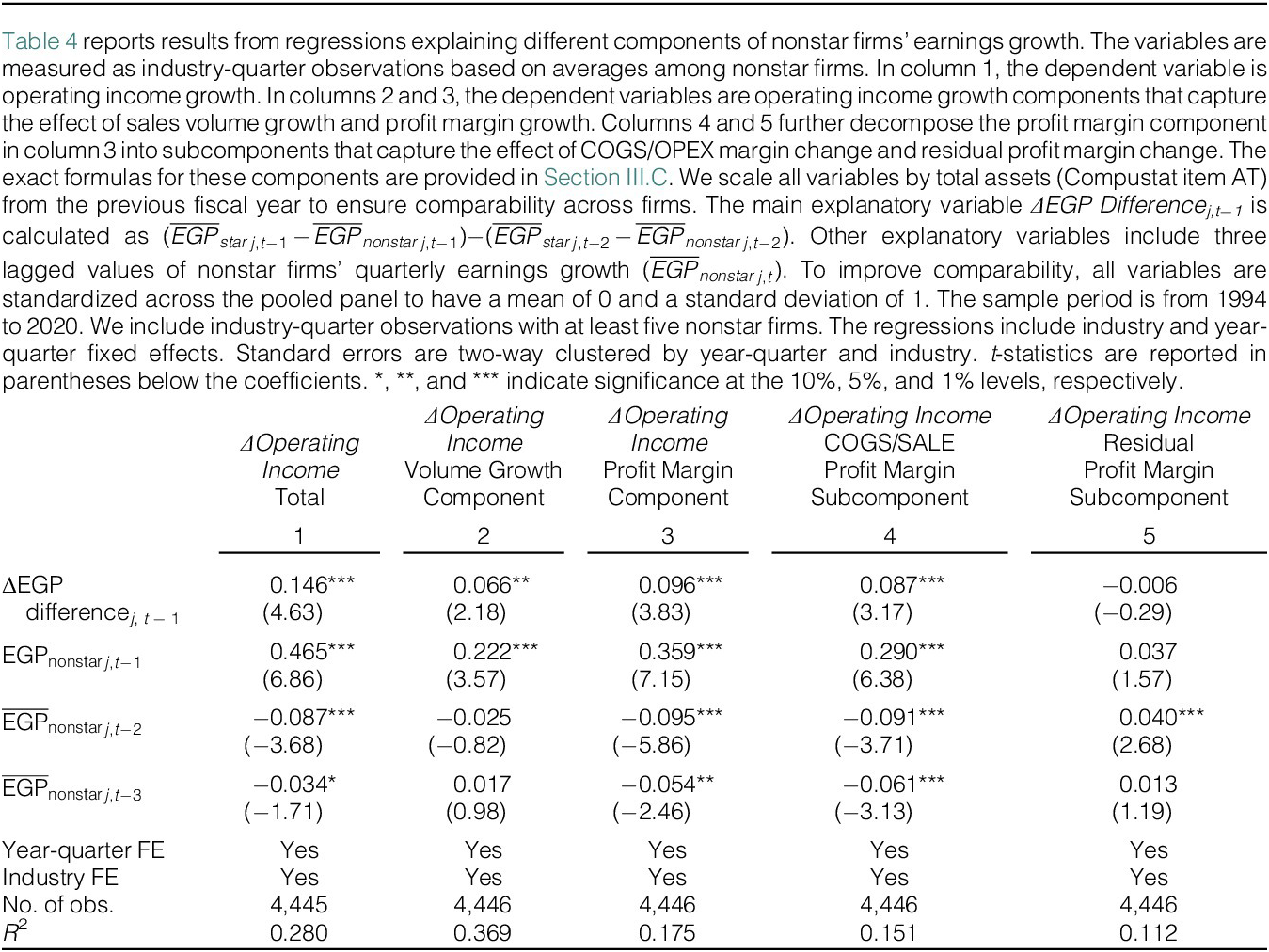
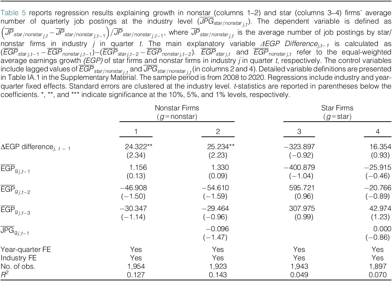
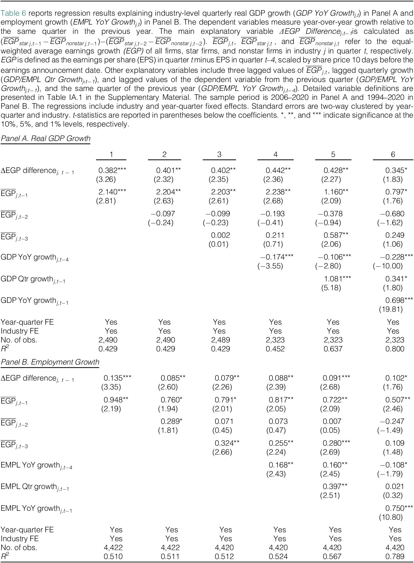
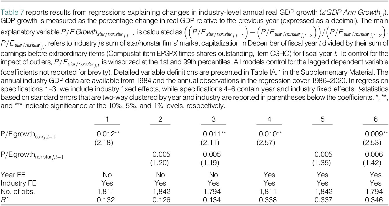
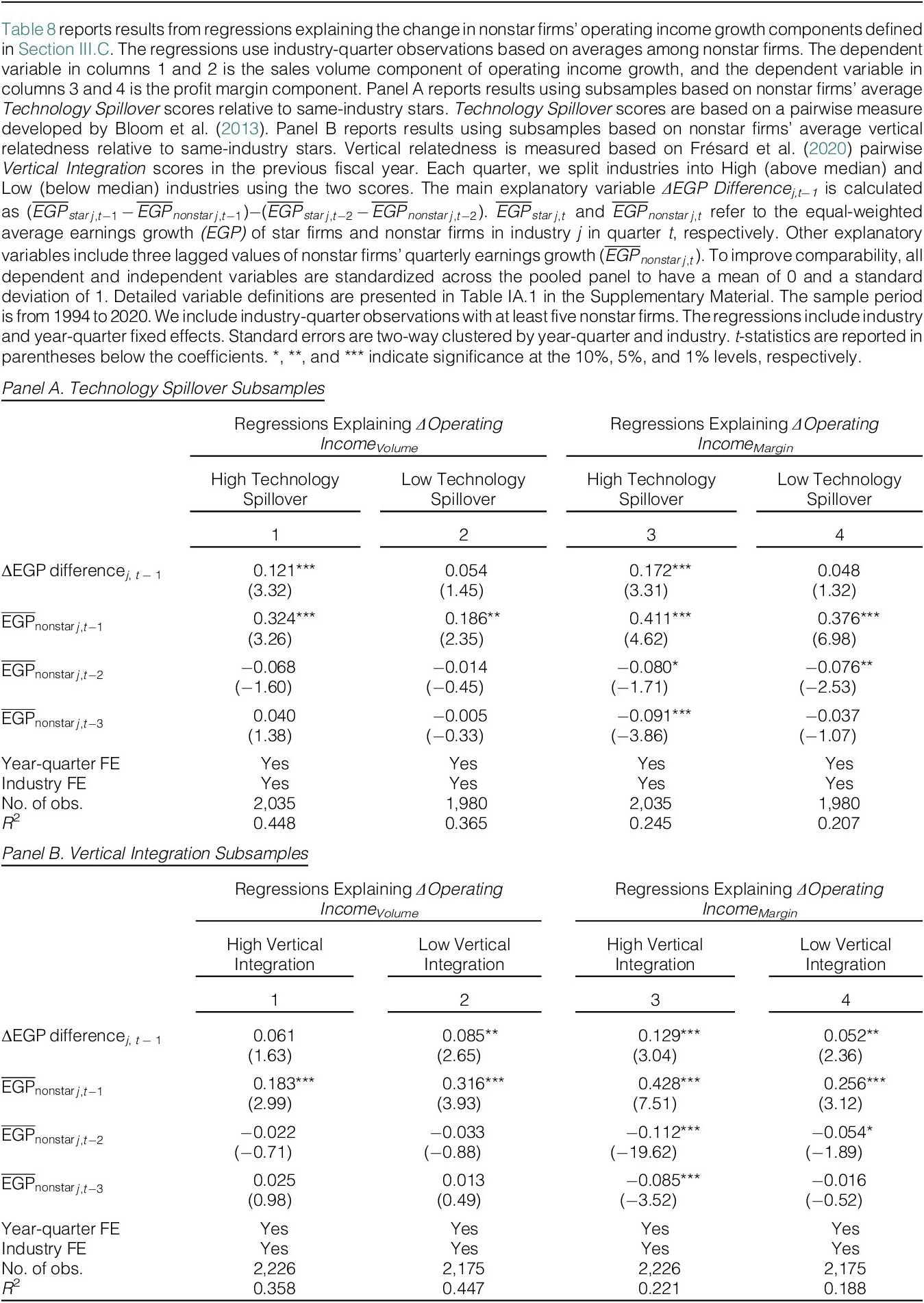
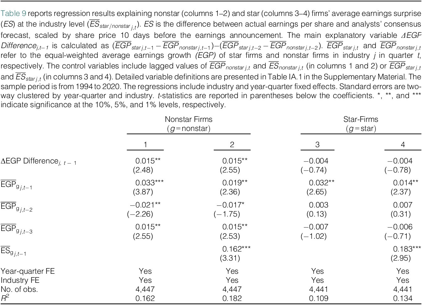
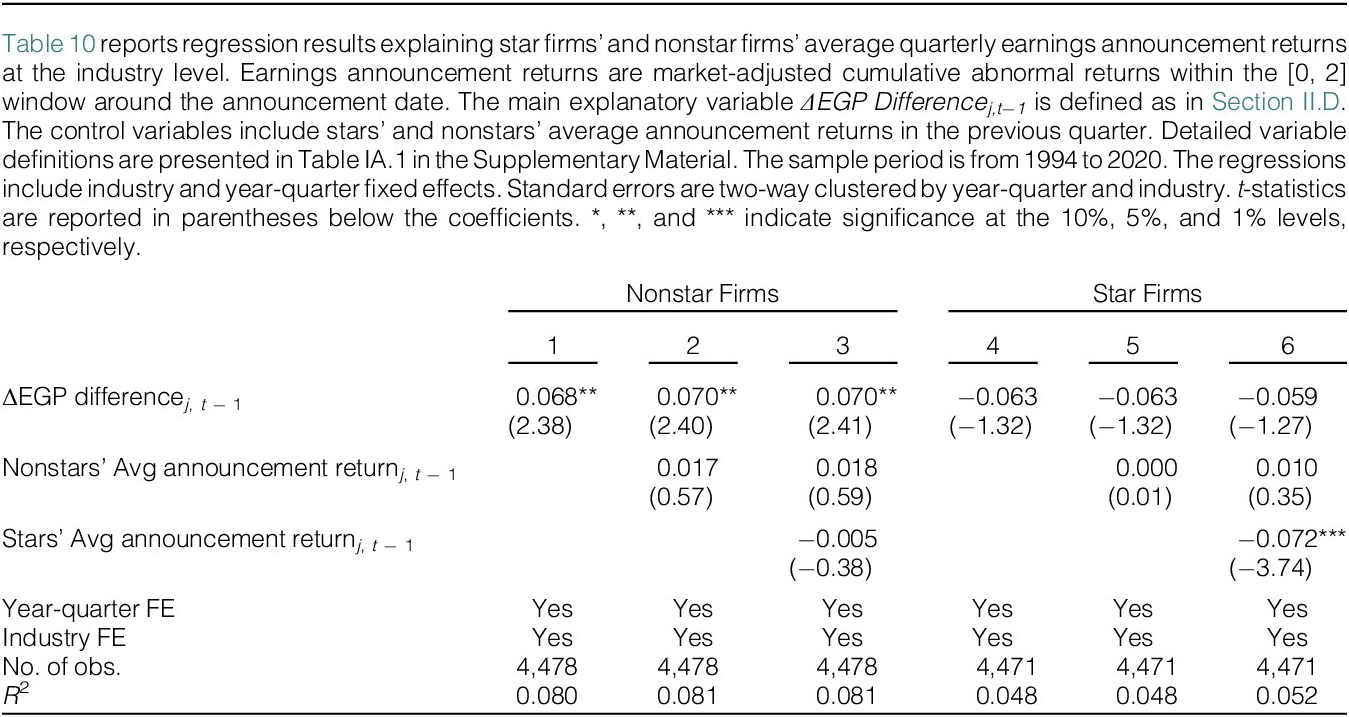
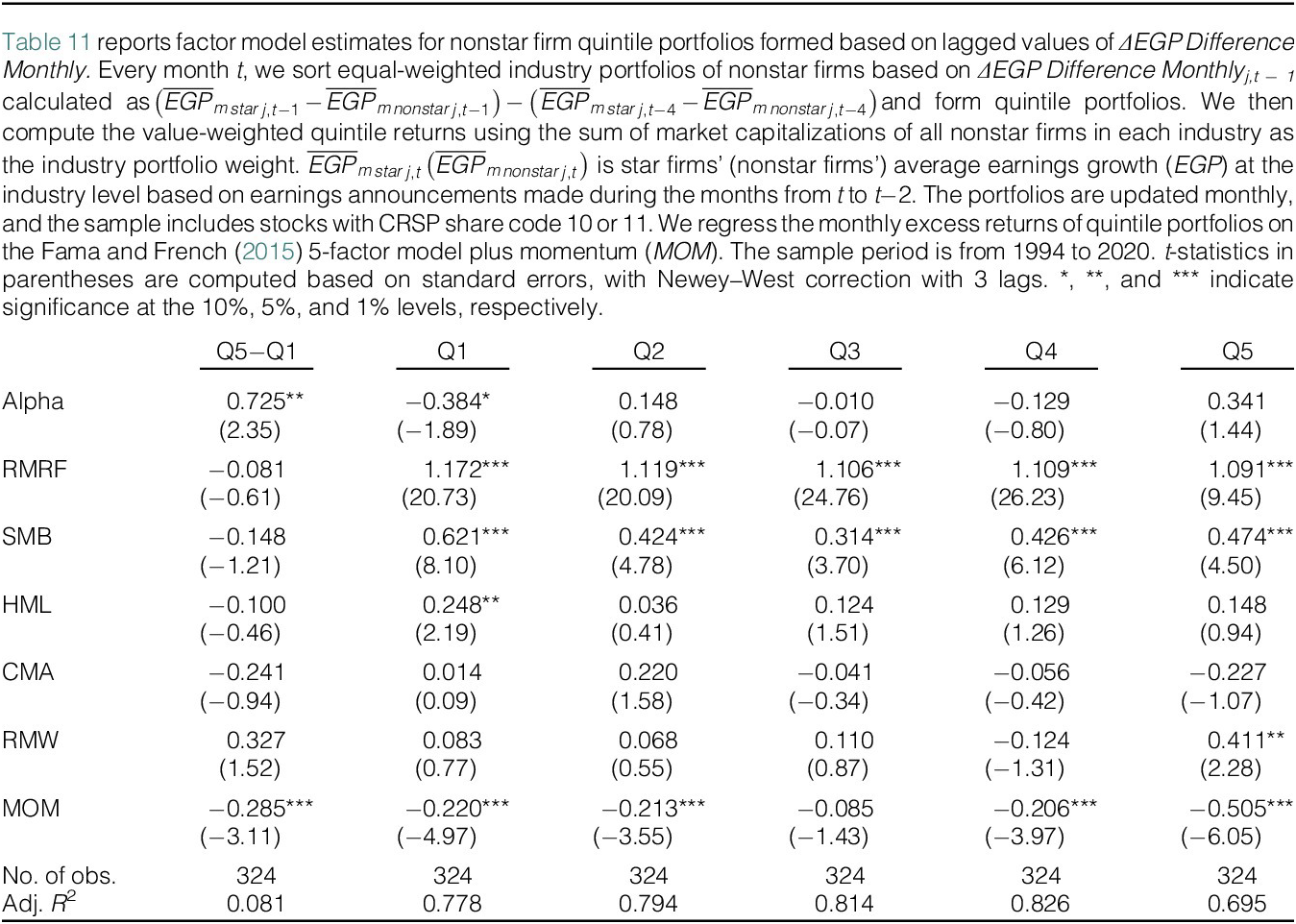
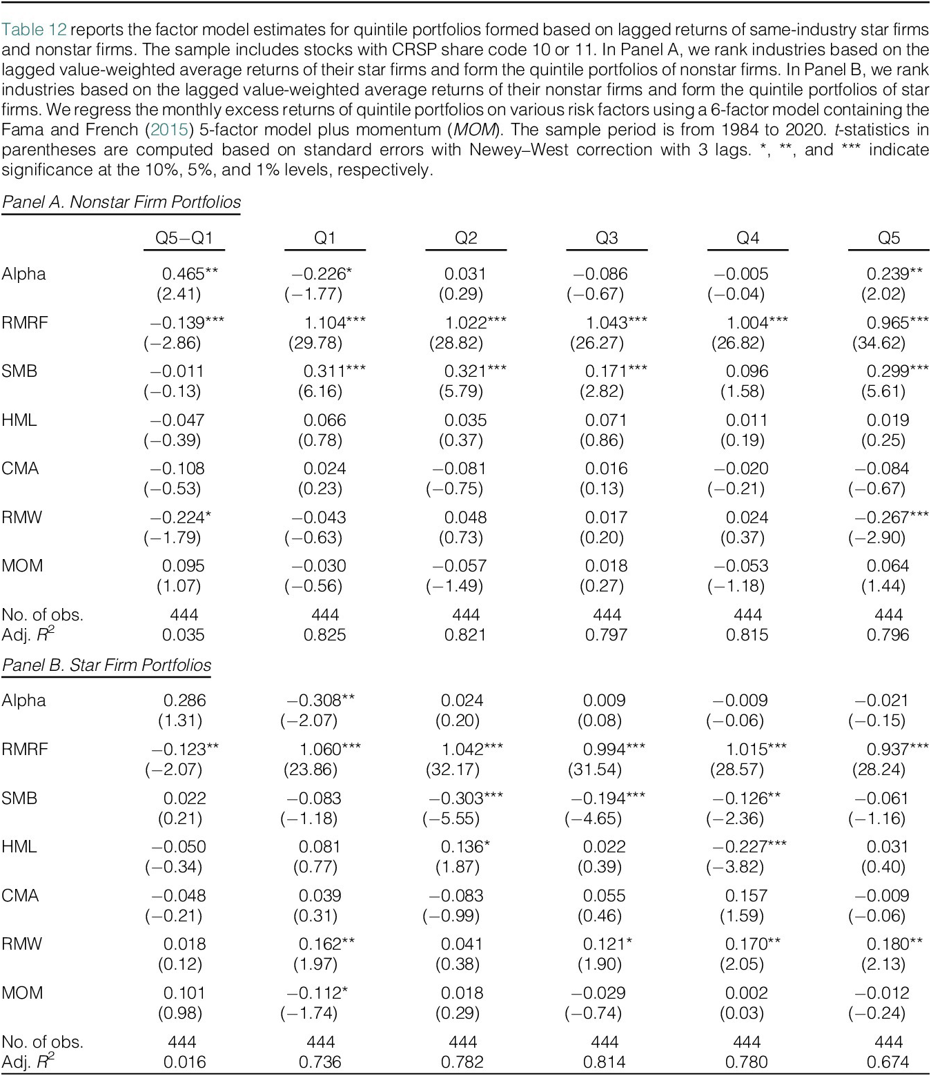


 Open access

