2.1 Large sieve with general sequences

Let $q \in \mathbb {Z}_+$ and consider the simplified version

(2.1) $$ \begin{align} \sum_{\lambda_j < 1/4} X^{2\theta_j} \left\vert \sum_{n \sim N} a_n\, \rho_{j\infty}(n) \right\vert^2 \lesssim \left(1 + \frac{N}{q}\right) \|a_n\|_2^2 \end{align} $$

of the large sieve inequality from Theorem 1.2, for $\mathfrak {a} = \infty $ , ignoring $(qN)^{o(1)}$ factors. Here $(a_n)$ are arbitrary complex coefficients, and the reader may pretend that $|a_n| \approx 1$ for each n, so that $\|a_n\|_2^2 \approx N$ . Such an inequality follows from [Reference Deshouillers and Iwaniec10, Theorem 2] when $X = 1$ , but we need larger values of X to temper the contribution of exceptional eigenvalues. The Kuznetsov trace formula [Reference Kuznetsov31] in Proposition 3.5, combined with large sieve inequalities for the regular spectrum [Reference Deshouillers and Iwaniec10, Theorem 2], essentially reduces the problem to bounding (a smoothed variant of) the sum

(2.2) $$ \begin{align} \sum_{\substack{c \sim NX \\ c \equiv 0 \pmod{q}}} \frac{1}{c} \sum_{m \sim N} \bar{a_m} \sum_{n \sim N} a_n\, S(m, n; c) \end{align} $$

by the same amount as in the right-hand side of (2.1) – see Corollary 3.10 for a formal statement in this direction. The left-hand side vanishes for $X < q/(2N)$ , so we immediately obtain (2.1) for $X \ll q/N$ , which is the content of [Reference Deshouillers and Iwaniec10, Theorem 5]. Alternatively, we can plug in the pointwise Weil bound for $S(m, n; c)$ and apply Cauchy–Schwarz, to obtain an upper bound of roughly

(2.3) $$ \begin{align} \frac{NX}{q} \frac{1}{NX} N \|a_n\|_2^2 \sqrt{NX} = \frac{N^{3/2} X^{1/2}}{q} \|a_n\|_2^2. \end{align} $$

This is acceptable in (2.1) provided that $X \le q^2/N^3$ , which completes the range from Theorem 1.2.

Improving the range $X \le \max (1, q/N, q^2/N^3)$ turns out to be quite difficult. Indeed, it is not clear how to exploit the averaging over c without the Kuznetsov formula, so any savings are more likely to come from bounding bilinear forms of Kloosterman sums $\sum _{m \sim N} a_m \sum _{n \sim N} b_n\, S(m, n; c)$ ; this is a notoriously hard problem for general sequences $(a_m), (b_n)$ [Reference Kowalski, Michel and Sawin29, Reference Kowalski, Michel and Sawin30, Reference Kerr, Shparlinski, Wu and Xi27, Reference Xi47]. For example, an extension of the work of Kowalski–Michel–Sawin [Reference Kowalski, Michel and Sawin29] to general moduli should improve Theorem 1.2 in the critical range $q \approx N^2$ , but even then the final numerical savings would be relatively small.

The other critical case encountered in applications is $q \approx N$ , where Theorem 1.2 gives no nontrivial savings in the $\theta $ -aspect (i.e., $X \ll 1$ ), and where such savings should in fact be impossible for general sequences $(a_n)$ . Indeed, we expect $|\rho _j(n)|$ to typically be of size $\approx q^{-1/2}$ , so by picking $a_n = q\, \bar {\rho _1(n)}$ , the left-hand side of (2.1) is at least $X^{2\theta (q)} N^2$ , while the right-hand side is $(1 + \frac {N}{q}) qN$ ; this limits the most optimistic savings for general sequences at $X = (1 + \frac {q}{N})^{1/(2\theta (q))}$ .

The key idea in our work is to make use of the special structure of the sequences $(a_n)$ which show up in variations of the dispersion method [Reference Linnik33]. Often, such sequences have sparse Fourier transforms, and using Fourier analysis on the corresponding exponential sums leads to a combinatorial problem.

2.2 Exponential phases and a counting problem

Let us focus on the case $a_n = e(n\alpha )$ , for some $\alpha \in [0, 1)$ . Expanding the Kloosterman sums from (2.2) and Fourier-completing in $m, n$ leads to a variant of the identity

(2.4)

Taking absolute values and ignoring the outer averaging over c, we are left with the task of bounding

(2.5)

for $c \sim NX$ , which is just a count of points on a modular hyperbola in short intervals (as considered in [Reference Cilleruelo and Garaev7]). When $\alpha = 0$ , one can directly use the divisor bound to write

up to a factor of $X^{o(1)}$ , which leads to a variant of

$$\begin{align*}\sum_{m,n \sim N} S(m, n; c) \lesssim c + N^2 = NX + N^2. \end{align*}$$

(This type of bound was also observed by Shparlinski and Zhang [Reference Shparlinski and Zhang43].) Overall, we roughly obtain

(2.6) $$ \begin{align} \sum_{\substack{c \sim NX \\ c \equiv 0 \pmod{q}}} \frac{1}{c} \sum_{m, n \sim N} S(m, n; c) \lesssim \frac{NX + N^2}{q}, \end{align} $$

which is at most $(1 + \frac {N}{q}) N$ , as required in (2.1), provided that

$$\begin{align*}X \le \max(N, q). \end{align*}$$

This gives the best-case range from (1.7) (when $a = 1$ ). The analogue of this argument for other values of $\alpha \in \mathbb {R}/\mathbb {Z}$ depends on the quality of the best rational approximations to $\alpha $ , due to a rescaling trick of Cilleruelo–Garaev [Reference Cilleruelo and Garaev7]. For an arbitrary value of $\alpha $ , a pigeonhole argument (Dirichlet approximation) leads to a bound of the shape

(2.7) $$ \begin{align} \sum_{\substack{c \sim NX \\ c \equiv 0 \pmod{q}}} \frac{1}{c} \sum_{m \sim N} e(-m\alpha) \sum_{n \sim N} e(n\alpha)\, S(m, n; c) \lesssim \frac{N^{3/2} X + N^2}{q}, \end{align} $$

and ultimately to the range $X \le \max (\sqrt {N}, q/\sqrt {N})$ , which is the worst (and average) case in (1.7) when $a = 1$ . Incorporating a scalar a inside $\rho _{j\infty }(an)$ is not too difficult, since a similar argument handles the analogous bilinear sums of $S(am, an; c)$ , up to a loss of $\gcd (a, c)$ .

2.3 Sequences with frequency concentration

It will probably not come as a surprise that one can extend the preceding discussion by Fourier-expanding other sequences $(a_n)$ , given a strong-enough concentration condition for their Fourier transforms, but there are some subtleties in how to do this optimally. If $a_n = \check {\mu }(n) = \int _{\mathbb {R}/\mathbb {Z}} e(n\alpha )\, d\mu (\alpha )$ for all $n \sim N$ and some bounded-variation complex measure $\mu $ , then there are at least two ways to proceed – depending on whether the integral over $\alpha $ is kept inside or outside of the square.

Indeed, by applying Cauchy–Schwarz in $\alpha $ and our Theorem 1.5 for exponential phases as a black-box, one can directly obtain a bound like

(2.8) $$ \begin{align} \sum_{\lambda_j < 1/4} X^{2\theta_j} \left\vert \sum_{n \sim N} a_n\, \rho_{j\mathfrak{a}}(n) \right\vert^2 \lesssim \left(1 + \frac{N}{q}\right) N |\mu|(\mathbb{R}/\mathbb{Z})^2, \end{align} $$

for all $X \le \max (\sqrt {N}, q/\sqrt {N})$ (and this range can be slightly improved given more information about the support of $\mu $ near rational numbers of small denominators). Unfortunately, this replaces the norm $\|a_n\|_2$ from Theorem 1.2 with $\sqrt {N} |\mu |(\mathbb {R}/\mathbb {Z})$ , which produces a significant loss unless $\mu $ is very highly concentrated – and it is difficult to make up for this loss through gains of $X^{2\theta }$ .

The alternative approach is to expand the square in the left-hand side of (2.8), pass to a sum of Kloosterman sums as in (2.2) by Kuznetsov, and only then Fourier-expand (two instances of) the sequence $(a_n)$ . Using similar combinatorial ideas as for (2.7), we can then essentially bound

(2.9) $$ \begin{align} \sum_{\substack{c \sim NX \\ c \equiv 0 \pmod{q}}} \frac{1}{c} \sum_{m \sim N} e(m\alpha) \sum_{n \sim N} e(n\beta)\, S(m, n; c) \lesssim \frac{N^{5/3} X + N^2}{q}, \end{align} $$

for arbitrary values of $\alpha , \beta \in \mathbb {R}/\mathbb {Z}$ . With no further information about the support of $\mu $ , this ultimately gives a bound like

$$\begin{align*}\sum_{\lambda_j < 1/4} X^{2\theta_j} \left\vert \sum_{n \sim N} a_n\, \rho_{j\mathfrak{a}}(n) \right\vert^2 \lesssim \left(1 + \frac{N}{q}\right) \|a_n\|_2^2 + \frac{N^{5/3}X + N^2}{q} |\mu|(\mathbb{R}/\mathbb{Z})^2, \end{align*}$$

which is acceptable in (2.1), in particular, whenever $X < N^{1/3}$ and $\sqrt {N} |\mu |(\mathbb {R}/\mathbb {Z}) \le \sqrt {q/N} \|a_n\|_2$ . Compared to the first approach, this generally gains less in the X-aspect, but it relaxes the concentration condition on $\mu $ if $N < q$ . This second approach turns out to be better for our applications; the resulting large sieve inequality is Theorem 5.2, which particularizes to Theorems 1.5 and 1.7.

What is perhaps more surprising, though, is that strong-enough frequency concentration (i.e., $\sqrt {N} |\mu |(\mathbb {R}/\mathbb {Z})^2 \le \sqrt {q/N} \|a_n\|_2$ ) arises in applications, beyond the case of exponential sequences. A key observation is that the aforementioned dispersion coefficients

(2.10) $$ \begin{align} a_n = \sum_{\substack{h_1, h_2 \sim H \\ h_1 \ell_1 - h_2 \ell_2 = n}} 1, \end{align} $$

with $\ell _1 \asymp \ell _2 \asymp L$ , come from a convolution of two “arithmetic progressions” . The Fourier transform of each of these two sequences has $\ell _i$ periodic peaks of height H and width $(H \ell _i)^{-1}$ , supported around multiples of $1/\ell _i$ . When $(\ell _1, \ell _2) = 1$ , multiplying these two Fourier transforms results in cancellation everywhere away from a small number ( $\le 1 + \frac {L}{H}$ ) of rational points (and thus, in frequency concentration on a set of size $\frac {1}{HL} + \frac {1}{H^2}$ ); see Lemma 4.11.

2.4 Multilinear forms of Kloosterman sums

Consider once again the sums (1.2), in the ranges

$$\begin{align*}M, N \le rs, \qquad\qquad X := \frac{s\sqrt{r} C}{\sqrt{MN}} \ge 1, \end{align*}$$

which are relevant for most applications. An additional use of the Kuznetsov formula, for the level $q = rs$ and the cusps $\infty , 1/s$ (with suitable scaling matrices), gives a variant of the bound

$$\begin{align*}\begin{aligned} &\sum_{m \sim M} a_m \sum_{n \sim N} b_n \sum_{(c, r) = 1} g\left(\frac{c}{C}\right) S(m\bar{r}, \pm n; sc) \\ &\quad\lesssim s\sqrt{r}C \sum_{\lambda_j < 1/4} X^{2\theta_j} \left\vert \sum_{m \sim M} a_m\, \rho_{j\infty}(m) \right\vert \left\vert \sum_{n \sim N} b_n\, \rho_{j\, 1/s}(n)\right\vert \ + \ \ldots \end{aligned} \end{align*}$$

Here we omitted the contribution of the regular Maass forms, Eisenstein series and holomorphic forms (which will not be dominant). A priori, this arrangement introduces a factor of $X^{2\theta (q)}$ in our bounds, recalling that $\theta (q) = \max _{\lambda _j(q) < 1/4} \theta _j(q)$ (if the maximum is nonempty, and $\theta (q) = 0$ otherwise). However, the value of X in this loss can be decreased through the large sieve inequalities for exceptional Maass forms. Indeed, after splitting $X = X_0 \sqrt {X_1 X_2}$ , taking out a factor of only $(1 + X_0)^{2\theta (q)}$ , and applying Cauchy–Schwarz, we reach

$$\begin{align*}s\sqrt{r}C\, (1 + X_0)^{2\theta(q)} \left(\sum_{\lambda_j < 1/4} X_1^{2\theta_j} \left\vert \sum_{m \sim M} a_m\, \rho_{j\infty}(m) \right\vert^2 \right)^{1/2} \left(\sum_{\lambda_j < 1/4} X_2^{2\theta_j} \left\vert \sum_{n \sim N} b_n\, \rho_{j\, 1/s}(n) \right\vert^2 \right)^{1/2}. \end{align*}$$

Above, we can choose $X_1$ and $X_2$ as the maximal values that can be fully incorporated in large sieve inequalities like (2.1) without producing losses in the right-hand side, for the specific sequences $(a_m)$ and $(b_n)$ . In this case, we roughly obtain a final bound of

$$\begin{align*}s\sqrt{r} C \left(1 + \frac{s\sqrt{r}C}{\sqrt{MN X_1 X_2}}\right)^{2\theta(q)} \|a_m\|_2\, \|b_n\|_2. \end{align*}$$

For example, if $a_m = e(m\alpha _{r,s})$ for some $\alpha _{r,s} \in \mathbb {R}/\mathbb {Z}$ , then we may take $X_1 = \max (\sqrt {N}, q/\sqrt {N})$ by Theorem 1.5, which ultimately saves a factor of $N^{\theta /2}$ . Similarly, if $(b_n)$ are of the form in (2.10), where $H \asymp L \asymp \sqrt {N}$ , then by Theorem 1.7 we may also take $X_2 = \max (\sqrt {N}, q/\sqrt {N})$ .

If some averaging over $r \sim R, s \sim S$ is available and the sequence $(a_m)$ does not depend on $r, s$ , then larger values of $X_1$ are available due to Deshouillers–Iwaniec [Reference Deshouillers and Iwaniec10, Theorems 6, 7]. In this setting, if $a_m = e(m\omega )$ for a fixed $\omega \in \mathbb {R}/\mathbb {Z}$ , one can combine the essentially-optimal value $X_1 = Q^2/N$ (see Theorem 3.11 below) with our savings in the $X_2$ -aspect. Following [Reference Deshouillers and Iwaniec10, Theorem 12], similar estimates can be deduced for multilinear forms of incomplete Kloosterman sums, simply by Fourier-completing them and appealing to the estimates for complete sums; see our Corollary 5.14. Such bounds feed directly into the dispersion method and its applications, as we shall see in Section 6.

2.5 Layout of paper

In Section 3, we cover notation and preliminary results, including several key lemmas from the spectral theory of automorphic forms. Section 4 only contains elementary arguments, from counting points on modular hyperbolas in Lemma 4.4 (following Cilleruelo–Garaev [Reference Cilleruelo and Garaev7]), to the bilinear Kloosterman bounds in Proposition 4.9 (which may be of independent interest to the reader). In Section 5.1, we combine these combinatorial inputs with the Deshouillers–Iwaniec setup [Reference Deshouillers and Iwaniec10] to prove a general large sieve inequality in Theorem 5.2, which can be viewed as our main technical result; we then deduce Theorems 1.5 and 1.7 from it. Section 5.3 contains the corollaries of these large sieve inequalities: various bounds for multilinear forms of Kloosterman sums, with improved dependencies on the $\theta $ parameter. Finally, in Section 6 we will use these bounds to prove Theorem 1.1, building on the work of Merikoski [Reference Merikoski37] and de la Bretèche–Drappeau [Reference de La Bretèche and Drappeau8].

3.1 Standard analytic notation

We write $\mathbb {Z}, \mathbb {Q}, \mathbb {R}, \mathbb {C}, {\mathbb {H}}$ for the sets of integers, rational numbers, real numbers, complex numbers, respectively complex numbers with positive imaginary part. We may scale these sets by constants, and may add the subscript $+$ to restrict to positive numbers; so for example $2\mathbb {Z}_+$ denotes the set of even positive integers, while $i\mathbb {R}$ is the imaginary line. For $\alpha \in \mathbb {R}$ (or $\mathbb {R}/\mathbb {Z}$ ), we denote $e(\alpha ) := \exp (2 \pi i \alpha )$ , and set $\|\alpha \| := \min _{n \in \mathbb {Z}} |\alpha - n|$ , which induces a metric on $\mathbb {R}/\mathbb {Z}$ . We write $\mathbb {Z}/c\mathbb {Z}$ for the ring of residue classes modulo a positive integer c, $(\mathbb {Z}/c\mathbb {Z})^\times $ for its multiplicative group of units, and $\bar {x}$ for the inverse of $x \in (\mathbb {Z}/c\mathbb {Z})^\times $ . We may use the latter notation inside congruences, with $x \equiv y\bar {z} \pmod {c}$ meaning that $xz \equiv y \pmod {c}$ (for $\gcd (z, c) = 1$ ). We may also use the notation $(a, b)$ for $\gcd (a, b)$ , and $[a, b]$ for $\mathrm {lcm}(a, b)$ , when it is clear from context to not interpret these as pairs or intervals. We write for the indicator function of a set S (or for the truth value of a statement S), $n \sim N$ for the statement that $N < n \le 2N$ (so, e.g., ), and interpret sums like $\sum _{n \sim N}$ , $\sum _{n \equiv 0 \pmod {q}}$ , or $\sum _{d \mid n}$ with the implied restrictions that $n, d \in \mathbb {Z}_+$ . For $n \in \mathbb {Z}_+$ , we define the divisor-counting function by $\tau (n) := \sum _{d \mid n} 1$ , and Euler’s totient function by . We say that a complex sequence $(a_n)$ is divisor-bounded iff $|a_n| \ll \tau (n)^{O(1)}$ . We also write $P^+(n)$ and $P^-(n)$ for the largest and smallest prime factors of a positive integer n, and recall that n is called y-smooth iff $P^+(n) \le y$ .

We use the standard asymptotic notation $f \ll g$ , $f \asymp g$ , $f = O(g)$ , $f = o_{x \to \infty }(g)$ from analytic number theory, and indicate that the implicit constants depend on some parameter $\varepsilon $ through subscripts (e.g., $f \ll _\varepsilon g$ , $f = O_\varepsilon (g)$ ). In particular, one should read bounds like $f(x) \ll x^{o(1)}$ as $\forall \varepsilon> 0, f(x) \ll _\varepsilon x^\varepsilon $ . Given $\ell \in \mathbb {Z}_+$ , we write $f^{(\ell )}$ for the $\ell $ th derivative of a function $f : \mathbb {R} \to \mathbb {C}$ , and $f^{(0)} = f$ . For $q \in [1, \infty ]$ , we denote by $\|f\|_{L^q}$ the $L^q$ -norm of a function $f : \mathbb {R} \to \mathbb {C}$ (or $f : \mathbb {R}/\mathbb {Z} \to \mathbb {C}$ ), and by $\|a\|_q$ (or $\|a_n\|_q$ ) the $\ell ^q$ norm of a sequence $(a_n)$ .

We require multiple notations for the Fourier transforms of $L^1$ functions $f, \Phi : \mathbb {R} \to \mathbb {C}$ , $\varphi : \mathbb {R}/\mathbb {Z} \to \mathbb {C}$ , and $a : \mathbb {Z} \to \mathbb {C}$ (the latter could be, e.g., a finite sequence $(a_n)_{n \sim N}$ extended with zeroes elsewhere). These are given by

(3.1) $$ \begin{align} \begin{aligned} f : \mathbb{R} \to \mathbb{C} \qquad \leadsto \qquad\,\, \hat{f} : \mathbb{C} \to \mathbb{C}, \qquad\quad &\hat{f}(\xi) := \int_{\mathbb{R}} f(t)\, e(-\xi t)\ dt, \\ \Phi : \mathbb{R} \to \mathbb{C} \qquad \leadsto \qquad\, \check{\Phi} : \mathbb{C} \to \mathbb{C}, \qquad\quad &\check{\Phi}(t) := \int_{\mathbb{R}} \Phi(\xi)\, e(\xi t)\ d\xi, \\ a : \mathbb{Z} \to \mathbb{C} \quad\ \ \, \, \leadsto \ \ \, \, \hat{a} : \mathbb{R}/\mathbb{Z} \to \mathbb{C}, \qquad\quad &\hat{a}(\alpha) := \sum_{n \in \mathbb{Z}} a_n\, e(-n\alpha), \qquad \\ \varphi : \mathbb{R}/\mathbb{Z} \to \mathbb{C} \qquad \leadsto \qquad \ \check{\varphi} : \mathbb{Z} \to \mathbb{C}, \qquad\quad &\check{\varphi}(n) := \int_{\mathbb{R}/\mathbb{Z}} \varphi(\alpha)\, e(n\alpha)\, d\alpha. \end{aligned} \end{align} $$

Note that the first two and the last two of these transforms are inverse operations under suitable conditions; in particular, if $\Phi $ is Schwarz, a is $L^1$ , and $\varphi $ is smooth (so $\check {\varphi }(n)$ decays rapidly as $|n| \to \infty $ ), one has

(3.2) $$ \begin{align} \check{\hat{\Phi}} \Big\vert_{\mathbb{R}} = \hat{\check{\Phi}} \Big\vert_{\mathbb{R}} = \Phi, \qquad\qquad \check{\hat{a}} = a, \qquad\qquad \hat{\check{\varphi}} = \varphi. \end{align} $$

We also denote the Fourier transform of a bounded-variation complex Borel measure $\mu $ on $\mathbb {R}/\mathbb {Z}$ by $\check {\mu }(n) := \int _{\mathbb {R}/\mathbb {Z}} e(n\alpha )\, d\mu (\alpha )$ . For instance, one has for the Lebesgue measure $\lambda $ , and $\check {\delta }_{A}(n) = \sum _{\alpha \in A} e(n\alpha )$ for the Dirac delta measure on a finite set $A \subset \mathbb {R}/\mathbb {Z}$ . Moreover, if $d\mu = \varphi \, d\lambda $ for some $L^1$ function $\varphi : \mathbb {R}/\mathbb {Z} \to \mathbb {C}$ , then $\check {\mu } = \check {\varphi }$ . Finally, with our notation, the Parseval–Plancherel identity reads $\|a_n\|_2^2 = \|\hat {a}\|_{L^2}^2$ (and $\|f\|_{L^2} = \|\hat {f}\|_{L^2}$ ), while Poisson summation states that for any Schwarz function f,

(3.3) $$ \begin{align} \sum_{n \in \mathbb{Z}} f(n) = \sum_{n \in \mathbb{Z}} \hat{f}(n) = \sum_{n \in \mathbb{Z}} \check{f}(n). \end{align} $$

In practice it will be useful to truncate the Poisson summation formula; we combine this with a smooth dyadic partition of unity and a separation of variables, in the following lemma.

Lemma 3.1 (Truncated Poisson with extra steps)

Let $x, N, Q \gg 1$ with $N, Q \ll x^{O(1)}$ , $q \asymp Q$ be a positive integer, $a \in \mathbb {Z}$ (or $\mathbb {Z}/q\mathbb {Z}$ ), and $\Phi : (0, \infty ) \to \mathbb {C}$ be a smooth function with $\Phi (t)$ supported in $t \asymp 1$ and $\Phi ^{(j)} \ll _j 1$ for $j \ge 0$ . Then for any $A, \delta> 0$ and $H := x^\delta N^{-1} Q$ , one has

$$\begin{align*}\begin{aligned} \sum_{n \equiv a \pmod{q}} \Phi\left(\frac{n}{N}\right) &= \frac{N}{q} \hat{\Phi}(0) + O_{A,\delta}\left(x^{-A}\right) \\ &\quad + \frac{N}{Q} \int \sum_{\substack{H_j = 2^j \\ 1 \le H_j \le H}} \sum_{\frac{1}{2} H_j \le |h| \le 2H_j} c_{j,u}(h)\, \Phi\left(\frac{uq}{Q}\right) e\left(\frac{ah}{q}\right) du, \end{aligned} \end{align*}$$

where the support of the integral in u is bounded, and

(3.4) $$ \begin{align} c_{j,u}(h) := \Psi_j\left(\frac{|h|}{H_j}\right) e\left(-h \frac{uN}{Q} \right), \end{align} $$

for some compactly-supported smooth functions $\Psi _j : (\frac {1}{2}, 2) \to \mathbb {C}$ with $\Psi _j^{(k)} \ll _k 1$ for $k \ge 0$ .

Proof. The Poisson identity (3.3) with a change of variables yields

$$\begin{align*}\sum_{n \equiv a \pmod{q}} \Phi\left(\frac{n}{N}\right) = \frac{N}{q} \sum_{h \in \mathbb{Z}} \hat{\Phi}\left(\frac{hN}{q}\right) e\left(\frac{ah}{q}\right). \end{align*}$$

We take out the main term at $h = 0$ , put $|h| \ge 1$ in dyadic ranges via a smooth partition of unity

and bound the contribution of $H_j> H = x^\delta N^{-1} Q$ by $O_{A,\delta }(x^{-A})$ using the Schwarz decay of $\Phi $ . In the remaining sum

$$\begin{align*}\begin{aligned} \frac{N}{q} \sum_{\substack{H_j = 2^j \\ 1 \le H_j \le H}} \sum_{\frac{1}{2}H_j \le |h| \le 2H_j} \Psi_j\left(\frac{|h|}{H_j}\right) \hat{\Phi}\left(\frac{hN}{q}\right) e\left(\frac{ah}{q}\right), \end{aligned} \end{align*}$$

we separate the $h, q$ variables via the Fourier integral

$$\begin{align*}\hat{\Phi}\left(\frac{hN}{q}\right) = \int \Phi(t)\, e\left(-h \frac{tN}{q}\right)\, dt = \frac{q}{Q} \int \Phi\left(\frac{uq}{Q}\right)\, e\left(-h \frac{uN}{Q}\right)\, du, \end{align*}$$

where we let $t = uq/Q$ . Swapping the (finite) sums with the integral completes our proof.

We also highlight the nonstandard Notation 4.1, pertaining to rational approximations. Further analytic notation specific to each section is described therein (see, for example, Notations 5.1, 6.2 and 6.7). For the rest of this section, we recount the main concepts relevant to bounding sums of Kloosterman sums via the Kuznetsov trace formula, mostly to clarify our notation (in particular, to point out small changes to the notation in [Reference Deshouillers and Iwaniec10]), and to explicitate a few useful lemmas.

3.2 Cusps, automorphic forms, Kloosterman sums

Recall that $\mathrm {PSL}_2(\mathbb {R}) := \mathrm {SL}_2(\mathbb {R})/\{\pm 1\}$ acts naturally on $\mathbb {C} \cup \{\infty \}$ by . For $q \in \mathbb {Z}_+$ , we denote by $\Gamma _0(q)$ the modular subgroup of level q, consisting of those matrices with $c \equiv 0 \pmod {q}$ . A number $\mathfrak {a} \in \mathbb {C} \cup \{\infty \}$ is called a cusp of $\Gamma _0(q)$ iff it is the unique fixed point of some $\sigma \in \Gamma _0(q)$ ; we write $\Gamma _{\mathfrak {a}} := \{ \sigma \in \Gamma _0(q) : \sigma \mathfrak {a} = \mathfrak {a}\}$ for the stabilizer of $\mathfrak {a}$ inside $\Gamma _0(q)$ . Two cusps are equivalent iff they lie in the same orbit of $\Gamma _0(q)$ ; the corresponding stabilizers are then conjugate inside $\Gamma _0(q)$ . By [Reference Deshouillers and Iwaniec10, Lemma 2.3], the fractions

(3.5) $$ \begin{align} \left\{\frac{u}{w}\ : \ u, w \in \mathbb{Z}_+,\ (u, w) = 1,\ w \mid q,\ u \le \gcd\left(w, \frac{q}{w}\right) \right\} \end{align} $$

form a maximal set of inequivalent cusps of $\Gamma _0(q)$ . Following [Reference Deshouillers and Iwaniec10, (1.1)], given a cusp $\mathfrak {a}$ of $\Gamma _0(q)$ and its equivalent representative $u/w$ from (3.5), we denote

(3.6) $$ \begin{align} \mu(\mathfrak{a}) := \frac{\gcd\left(w, \frac{q}{w}\right)}{q}, \end{align} $$

(Like most of our notation involving cusps, this implicitly depends on the level q as well.) In particular, the cusp at $\infty $ of $\Gamma _0(q)$ is equivalent to the fraction $1/q$ , so we have $\mu (\infty ) = q^{-1}$ . More generally, we have $\mu (1/s) = q^{-1}$ whenever $q = rs$ with $\gcd (r, s) = 1$ , and it is these cusps which account for most applications to sums of Kloosterman sums; thus for simplicity, we restrict all of our main results to cusps with $\mu (\mathfrak {a}) = q^{-1}$ . Following [Reference Deshouillers and Iwaniec10, (1.2)], a scaling matrix $\sigma _{\mathfrak {a}}$ for a cusp $\mathfrak {a}$ is an element of $\mathrm {PSL}_2(\mathbb {R})$ such that

(3.7)

Scaling matrices will allow us to expand $\Gamma _{\mathfrak {a}}$ -invariant functions $f : {\mathbb {H}} \to \mathbb {C}$ as Fourier series around the cusp $\mathfrak {a}$ , via the change of coordinates $z \gets \sigma _{\mathfrak {a}} z$ (note that if f is $\Gamma _{\mathfrak {a}}$ -invariant, then $z \mapsto f(\sigma _{\mathfrak {a}} z)$ is $\Gamma _\infty $ -invariant). For a given cusp $\mathfrak {a}$ , the choice of $\sigma _{\mathfrak {a}}$ can only vary by simple changes of coordinates

(3.8)

for $\alpha \in \mathbb {R}$ (which result in multiplying the Fourier coefficients by exponential phases $e(n\alpha )$ ). When $\mu (\mathfrak {a}) = q^{-1}$ , we must have $\mathfrak {a} = \tau (1/s)$ for some $\tau \in \Gamma _0(q)$ and $rs = q$ with $(r, s) = 1$ ; in this case, inspired by Watt [Reference Watt46, p. 195], we will use the canonical choice of scaling matrix

(3.9)

where $\bar {r}, \bar {s}$ are integers such that $r\bar {r} + s\bar {s} = 1$ (for definiteness, let us say we pick $\bar {s} \ge 0$ to be minimal). This is different from the choice in [Reference Deshouillers and Iwaniec10, (2.3)], and leads to the simplification of certain extraneous exponential phases. For the cusp , (3.9) reduces back to the identity matrix.

We refer the reader to the aforementioned work of Deshouillers–Iwaniec [Reference Deshouillers and Iwaniec10] for a brief introduction to the classical spectral theory of $\mathrm {GL}_2$ automorphic forms, to [Reference Iwaniec25, Reference Iwaniec24, Reference Iwaniec and Kowalski26] for a deeper dive into this topic, to [Reference Drappeau14, Reference Topacogullari45, Reference Drappeau, Pratt and Radziwiłł15, Reference de La Bretèche and Drappeau8, Reference Lichtman32, Reference Pascadi39] for follow-up works and optimizations, and to [Reference Bump6] for the modern viewpoint of automorphic representations. For our purposes, an automorphic form of level q and integer weight $k \ge 0$ will be a smooth function $f : {\mathbb {H}} \to \mathbb {C}$ satisfying the transformation law

as well as moderate (at-most-polynomial) growth conditions near every cusp. We say that f is square-integrable iff $\left \langle f, f \right \rangle _k < \infty $ , where $\left \langle f, g \right \rangle _k := \iint _{\Gamma _0(q) \backslash {\mathbb {H}}} f(x+iy)\, \bar {g(x+iy)}\, y^{k-2}\, dx\, dy$ is the Petersson inner product. We denote by $L^2(\Gamma _0(q) \backslash {\mathbb {H}}, k)$ the space of square-integrable automorphic forms of level q and weight k; when we drop the dependency on k, it should be understood that $k = 0$ . Finally, we call f a cusp form iff it is square-integrable and vanishes at all cusps.

Kloosterman sums show up in the Fourier coefficients of Poincaré series, which are useful in detecting the Fourier coefficients of other automorphic forms via inner products (see [Reference Deshouillers and Iwaniec10, (1.8), (1.18)]). In fact, by Fourier expanding a Poincaré series corresponding to a cusp $\mathfrak {a}$ around another cusp $\mathfrak {b}$ , one is led to a more general family of Kloosterman-type sums, depending on both $\mathfrak {a}$ and $\mathfrak {b}$ .

More specifically (following [Reference Deshouillers and Iwaniec10, (1.3)], [Reference Drappeau14, §4.1.1], [Reference Iwaniec24]), given two cusps $\mathfrak {a}, \mathfrak {b}$ of $\Gamma _0(q)$ , we first let

Here $\sigma _{\mathfrak {a}}$ and $\sigma _{\mathfrak {b}}$ are arbitrary scaling matrices for $\mathfrak {a}$ and $\mathfrak {b}$ , but the set $\mathcal {C}_{\mathfrak {a}\mathfrak {b}}$ actually depends only on $\mathfrak {a}$ and $\mathfrak {b}$ (since multiplication by matrices does not affect the bottom-left entry). Then we let

for any $c \in \mathbb {R}_+$ (although this is only nonempty when $c \in \mathcal {C}_{\mathfrak {a} \mathfrak {b}}$ ). By this definition, the set $\mathcal {D}_{\mathfrak {a}\mathfrak {b}}(c)$ is finite, does not depend on $\sigma _{\mathfrak {a}}$ , and only depends on $\sigma _{\mathfrak {b}}$ up to translations. It turns out that a given $\tilde {d} \in \mathcal {D}_{\mathfrak {a} \mathfrak {b}}(c)$ uniquely determines the value of $\tilde {a} \in \mathbb {R}/c\mathbb {Z}$ such that for some $a \in \tilde {a}$ , $d \in \tilde {d}$ (see [Reference Deshouillers and Iwaniec10, p. 239]). Symmetrically, this $\tilde {a}$ does not depend on $\sigma _{\mathfrak {b}}$ , and only depends on $\sigma _{\mathfrak {a}}$ up to translations. Thus given $c \in \mathbb {R}_+$ and $m, n \in \mathbb {Z}$ , it makes sense to define

(3.10) $$ \begin{align} S_{\mathfrak{a} \mathfrak{b}}(m, n; c) := \sum_{\tilde{d} \in \mathcal{D}_{\mathfrak{a} \mathfrak{b}}(c)} e\left(\frac{m \tilde{a} + n \tilde{d}}{c}\right), \end{align} $$

where $\tilde {a}$ and $\tilde {d}$ are corresponding values mod c; note that this vanishes unless $c \in \mathcal {C}_{\mathfrak {a}\mathfrak {b}}$ . Since varying the choices of $\sigma _{\mathfrak {a}}$ and $\sigma _{\mathfrak {b}}$ has the effect of uniformly translating $\tilde {a}$ , respectively $\tilde {d}$ , it follows that $S_{\mathfrak {a} \mathfrak {b}}(m, n; c)$ only depends on $\sigma _{\mathfrak {a}}, \sigma _{\mathfrak {b}}$ up to multiplication by exponential phases $e(m\alpha )$ , $e(n\beta )$ . In fact, the same holds true when varying $\mathfrak {a}$ and $\mathfrak {b}$ in equivalence classes of cusps [Reference Deshouillers and Iwaniec10, p. 239]. We also note the symmetries

(3.11) $$ \begin{align} S_{\mathfrak{a}\mathfrak{b}}(m, -n; c) = \bar{S_{\mathfrak{a}\mathfrak{b}}(-m, n; c)}, \qquad\qquad S_{\mathfrak{a}\mathfrak{b}}(m, n; c) = \bar{S_{\mathfrak{b}\mathfrak{a}}(n, m; c)}, \end{align} $$

the second one following from the fact that

Let us now relate these sums to the classical Kloosterman sums from (1.1).

Lemma 3.2 (Explicit Kloosterman sums [Reference Watt46])

Let $q = rs$ with $r, s \in \mathbb {Z}_+$ , $\gcd (r, s) = 1$ . Then for any $c \in \mathbb {R}_+$ and $m, n \in \mathbb {Z}$ , with the choice of scaling matrices from (3.9), one has

(3.12)

Moreover, let $\mathfrak {a}$ be any cusp of $\Gamma _0(q)$ with $\mu (\mathfrak {a}) = q^{-1}$ , and $\sigma _{\mathfrak {a}}$ be as in (3.9). Then one has

(3.13)

Varying the choice of scaling matrix as in (3.8) would result in an additional factor of $e((n-m)\alpha )$ .

3.3 The Kuznetsov formula and exceptional eigenvalues

We now recognize some important classes of $\mathrm {GL}_2$ automorphic forms of level q:

1. (1). Classical modular forms, which are holomorphic with removable singularities at all cusps, and can only have even weights $k \in 2\mathbb {Z}_+$ (except for the zero form). A holomorphic cusp form f additionally vanishes at all cusps; such forms have Fourier expansions

   (3.14) $$ \begin{align} j(\sigma_{\mathfrak{a}}, z)^{-k} f(\sigma_{\mathfrak{a}} z) = \sum_{n=1}^\infty \psi_{\mathfrak{a}}(n)\, e(n z) \end{align} $$

   around each cusp $\mathfrak {a}$ of $\Gamma _0(q)$ (see [Reference Deshouillers and Iwaniec10, (1.7)]). We mention that the space of holomorphic cusp forms of weight k is finite-dimensional, and denote its dimension by $h_k = h_k(q)$ .

2. (2). Maass forms (of weight $0$ ), which are invariant under the action of $\Gamma _0(q)$ , and are eigenfunctions of the hyperbolic Laplacian $\Delta = -y^2 \left (\partial _x^2 + \partial _y^2\right )$ . These include:

   1. (a). Maass cusp forms, which additionally vanish at all cusps and are square-integrable. These (plus the constant functions) correspond to the discrete spectrum of the hyperbolic Laplacian on $L^2\left (\Gamma _0(q) \backslash {\mathbb {H}}\right )$ , consisting of eigenvalues $0 = \lambda _0 < \lambda _1 \le \lambda _2 \le \lambda _3 \le \ldots $ with no limit point. Around a given cusp $\mathfrak {a}$ , Maass cusp forms have Fourier expansions (see [Reference Deshouillers and Iwaniec10, (1.15)])

      (3.15) $$ \begin{align} u(\sigma_{\mathfrak{a}} z) = y^{1/2} \sum_{n \neq 0} \rho_{\mathfrak{a}}(n) K_{i\kappa}(2\pi |n| y)\, e(mx), \end{align} $$

      where $z = x + iy$ and K is the Whittaker function normalized as in [Reference Deshouillers and Iwaniec10, p. 264].

   2. (b). Eisenstein series, explicitly defined by $E_{\mathfrak {a}}(z; s) := \sum _{\tau \in \Gamma _{\mathfrak {a}} \backslash \Gamma _0(q)} {\mathrm {Im}}^s\left (\sigma _{\mathfrak {a}}^{-1} \tau z\right )$ for ${\mathrm {Re}}\, s> 1$ , and meromorphically continued to $s \in \mathbb {C}$ . Although not square-integrable themselves, “incomplete” versions of Eisenstein series with $s = \frac {1}{2} + ir$ (and $r \in \mathbb {R}$ ) can be used to describe the orthogonal complement in $L^2\left (\Gamma _0(q) \backslash {\mathbb {H}}\right )$ of the space of Maass cusp forms, corresponding to the continuous spectrum of the hyperbolic Laplacian. Sharing similarities with both Maass cusp forms and Poincaré series, the Eisenstein series $E_{\mathfrak {a}}$ have Fourier expansions [Reference Deshouillers and Iwaniec10, (1.17)] around any cusp $\mathfrak {b}$ , involving the Whittaker function and the Kloosterman-resembling coefficients (for $n \in \mathbb {Z}$ , $n \neq 0$ )

      (3.16) $$ \begin{align} \varphi_{\mathfrak{a}\mathfrak{b}}(n; s) := \sum_{c \in \mathcal{C}_{\mathfrak{a}\mathfrak{b}}} c^{-2s} \sum_{\tilde{d} \in \mathcal{D}_{\mathfrak{a}\mathfrak{b}}(c)} e\left(\frac{n \tilde{d}}{c}\right). \end{align} $$

We are particularly interested in the exceptional Maass cusp forms, which have eigenvalues $\lambda _j \in (0, 1/4)$ ; there can only be finitely many such forms of each level q, and Selberg conjectured [Reference Selberg41] that there are none. With implicit dependencies on q, we denote

(3.17) $$ \begin{align} \kappa_j^2 := \lambda_j - \frac{1}{4} \qquad\qquad \text{and} \qquad\qquad \theta_j := i \kappa_j, \end{align} $$

where $\kappa _j$ is chosen such that $i \kappa _j> 0$ or $\kappa _j \ge 0$ ; thus exceptional forms correspond to imaginary values of $\kappa _j$ and positive values of $\theta _j$ . Letting

$$\begin{align*}\theta(q) := \sqrt{\max\left(0, \tfrac{1}{4} - \lambda_1(q)\right)} = \begin{cases} \theta_1(q), & \theta_1(q)> 0 \\ 0, & \text{otherwise}. \end{cases}, \qquad\qquad \theta_{\max} := \sup_{q \ge 1}\, \theta(q), \end{align*}$$

Selberg’s eigenvalue conjecture asserts that $\theta _{\max } = 0$ , and the best result towards it is due to Kim–Sarnak [Reference Kim28, Appendix 2]. This deep unconditional result requires the theory of $\mathrm {GL}_n$ automorphic representations [Reference Bump6], but it is a very useful black-box input to spectral methods, where various bounds have exponential dependencies on $\theta $ .

Based on earlier work of Kuznetsov [Reference Kuznetsov31], Deshouillers–Iwaniec [Reference Deshouillers and Iwaniec10] developed a trace formula relating weighted sums over c of the generalized Kloosterman sums from (3.10) to (sums of products of) the Fourier coefficients of holomorphic cusp forms, Maass cusp forms, and Eisenstein series, around any two cusps $\mathfrak {a}, \mathfrak {b}$ of $\Gamma _0(q)$ . Roughly speaking, this follows by summing two applications of Parseval’s identity for the aforementioned Poincaré series: one in the space of holomorphic cusp forms (summing over all weights $k \in 2\mathbb {Z}_+$ ), and one in the space of square-integrable automorphic forms of weight $0$ , via the spectral decomposition of the hyperbolic Laplacian (leading to the terms from Maass cusp forms and Eisenstein series).

One can arrange the resulting Kuznetsov trace formula so that the Kloosterman sums in the left-hand side are weighted by an arbitrary compactly-supported smooth function $\varphi $ ; in the right-hand side, the Fourier coefficients of automorphic forms are consequently weighted by Bessel transforms of $\varphi $ , defined for $r \in \mathbb {R} \setminus \{0\}$ by

(3.18) $$ \begin{align} \begin{aligned} \tilde{\mathcal{B}}_\varphi(r) &:= \int_0^\infty J_r(y)\, \varphi(y) \frac{dy}{y}, \\ \hat{\mathcal{B}}_\varphi(r) &:= \frac{\pi}{\sinh(\pi r)} \int_0^\infty \frac{J_{2ir}(x) - J_{-2ir}(x)}{2i} \varphi(x) \frac{dx}{x}, \\ \check{\mathcal{B}}_\varphi(r) &:= \frac{4}{\pi} \cosh(\pi r) \int_0^\infty K_{2ir}(x)\, \varphi(x) \frac{dx}{x}, \end{aligned} \end{align} $$

where $K_{it}$ is the aforementioned Whittaker function, and the Bessel functions $J_\ell $ , $J_{it}$ are defined as in [Reference Deshouillers and Iwaniec10, p. 264–265] (above we slightly departed from the notation in [Reference Deshouillers and Iwaniec10, Reference Drappeau14], to avoid confusion with Fourier transforms). All we will need to know about these transforms are the following bounds.

Lemma 3.4 (Bessel transform bounds [Reference Deshouillers and Iwaniec10])

Let $Y> 0$ and $\varphi : \mathbb {R} \to \mathbb {C}$ be a smooth function with compact support in $y \asymp Y$ , satisfying $\varphi ^{(j)}(y) \ll _j Y^{-j}$ for $j \ge 0$ . Then one has

(3.19) $$ \begin{align} \hat{\mathcal{B}}_\varphi(ir),\ \check{\mathcal{B}}_{\varphi}(ir) &\ll \frac{1 + Y^{-2r}}{1+Y}, \qquad\qquad\ \ \text{ for }\ 0 < r < \frac{1}{2}, \end{align} $$

(3.20) $$ \begin{align} \tilde{\mathcal{B}}_\varphi(r),\ \hat{\mathcal{B}}_\varphi(r),\ \check{\mathcal{B}}_{\varphi}(r) &\ll \frac{1 + |\log Y|}{1+Y}, \qquad\qquad \text{ for }\ r \in \mathbb{R} \setminus \{0\}, \end{align} $$

(3.21) $$ \begin{align} \tilde{\mathcal{B}}_\varphi(r),\ \hat{\mathcal{B}}_\varphi(r),\ \check{\mathcal{B}}_{\varphi}(r) &\ll |r|^{-5/2} + |r|^{-3}Y, \qquad \text{ for }\ r \in \mathbb{R},\ |r| \ge 1, \end{align} $$

Moreover, if $\varphi $ is nonnegative with $\int \varphi (y)\, dy \gg Y$ , and $Y < c$ for some constant $c \ll 1$ (depending on the implied constants so far), then one has

(3.22) $$ \begin{align} \hat{\mathcal{B}}_\varphi(\kappa) &\ll (\kappa^2+1)^{-1}, \qquad \text{ for }\ \kappa \in \mathbb{R} \setminus \{0\}, \end{align} $$

(3.23) $$ \begin{align} \hat{\mathcal{B}}_\varphi(\kappa) &\asymp Y^{-2i\kappa}, \qquad\qquad \, \text{ for }\ 0 < i \kappa < \frac{1}{2}. \end{align} $$

Finally, let us state the Kuznetsov trace formula, following the notation of Deshouillers–Iwaniec [Reference Deshouillers and Iwaniec10].

Proposition 3.5 (Kuznetsov trace formula [Reference Deshouillers and Iwaniec10, Reference Kuznetsov31])

Let $\varphi : \mathbb {R} \to \mathbb {C}$ be a compactly-supported smooth function, $q \in \mathbb {Z}_+$ , and $\mathfrak {a}, \mathfrak {b}$ be cusps of $\Gamma _0(q)$ . Then for any positive integers $m, n$ and $\mathrm {sgn} \in \{1, -1\}$ , one has

(3.24) $$ \begin{align} \sum_{c \in \mathcal{C}_{\mathfrak{a}\mathfrak{b}}} \frac{S_{\mathfrak{a}\mathfrak{b}}(m, \mathrm{sgn}\cdot n; c)}{c} \varphi \left(\frac{4 \pi \sqrt{mn}}{c}\right) = \begin{cases} \mathcal{H} + \mathcal{M} + \mathcal{E}, & \mathrm{sgn} = 1, \\ \mathcal{M}' + \mathcal{E}', & \mathrm{sgn} = -1, \end{cases} \end{align} $$

with the following notations. Firstly, the holomorphic contribution is

(3.25) $$ \begin{align} \mathcal{H} = \frac{1}{2\pi} \sum_{k \in 2\mathbb{Z}_+} \tilde{\mathcal{B}}_\varphi(k-1) \frac{i^k (k-1)!}{(4\pi \sqrt{mn})^{k-1}} \sum_{j = 1}^{h_k(q)} \bar{\psi_{jk\mathfrak{a}}(m)}\, \psi_{jk\mathfrak{b}}(n), \end{align} $$

for any orthonormal bases of level-q holomorphic cusp forms $(f_{jk})_j$ of weight $k \in 2\mathbb {Z}_+$ , with Fourier coefficients $\psi _{jk\mathfrak {a}}(n)$ as in (3.14). Secondly, the Maass contributions are

(3.26) $$ \begin{align} \mathcal{M} = \sum_{j = 1}^\infty \frac{\hat{\mathcal{B}}_\varphi(\kappa_j)}{\cosh(\pi \kappa_j)}\, \bar{\rho_{j\mathfrak{a}}(m)}\, \rho_{j\mathfrak{b}}(n), \qquad\quad \mathcal{M}' = \sum_{j = 1}^\infty \frac{\check{\mathcal{B}}_\varphi(\kappa_j)}{\cosh(\pi \kappa_j)}\, \rho_{j\mathfrak{a}}(m)\, \rho_{j\mathfrak{b}}(n), \end{align} $$

for any orthonormal basis $(u_j)_j$ of level-q Maass cusp forms, with eigenvalues $\lambda _j$ (and $\kappa _j, \theta _j$ as in (3.17)), and Fourier coefficients $\rho _{j\mathfrak {a}}(n)$ as in (3.15). Thirdly, the Eisenstein contributions are

(3.27) $$ \begin{align} \begin{aligned} \mathcal{E} &= \frac{1}{\pi} \sum_{\mathfrak{c}} \int_{-\infty}^\infty \hat{\mathcal{B}}_\varphi(r)\left(\frac{m}{n}\right)^{-ir} \bar{\varphi_{\mathfrak{c}\mathfrak{a}}\left(m; \frac{1}{2} + ir\right)} \varphi_{\mathfrak{c}\mathfrak{b}}\left(n; \frac{1}{2} + ir\right)\, dr, \\ \mathcal{E}' &= \frac{1}{\pi} \sum_{\mathfrak{c}} \int_{-\infty}^\infty \check{\mathcal{B}}_\varphi(r)\left(mn\right)^{ir} \varphi_{\mathfrak{c}\mathfrak{a}}\left(m; \frac{1}{2} + ir\right) \varphi_{\mathfrak{c}\mathfrak{b}}\left(n; \frac{1}{2} + ir\right)\, dr, \end{aligned} \end{align} $$

where the Fourier coefficients $\varphi _{\mathfrak {a}\mathfrak {b}}(n; s)$ are as in (3.16), and $\mathfrak {c}$ varies over the cusps of $\Gamma _0(q)$ .

Remark 3.6. Upon inspecting the Maass contribution (3.26) in light of the bounds (3.19) and (3.23), the losses due to the exceptional spectrum are apparent. Indeed, if $\varphi (y)$ is supported in $y \asymp Y \asymp \frac {\sqrt {mn}}{C}$ for some $C> 0$ (indicating the size of c), then the Bessel transforms bounds for exceptional eigenvalues are (a priori) worse by a factor of

$$\begin{align*}\max\left(1, Y^{-2\theta(q)}\right) \asymp \left(1 + \frac{C}{\sqrt{mn}}\right)^{2\theta(q)}, \end{align*}$$

compared to the regular (nonexceptional) spectrum.

3.4 Bounds for Fourier coefficients

If one is interested in a particular holomorphic or Maass cusp form (ideally, a Hecke eigenform), then various bounds for its Fourier coefficients follow from the theory of automorphic representations and their L-functions [Reference Deshouillers and Iwaniec10, Reference Sarnak40, Reference Kim28, Reference Bump6, Reference Goldfeld and Hundle19, Reference Goldfeld and Hundley20]. Here we are interested in bounding averages over bases of automorphic forms, resembling those that show up in (3.25) to (3.27); naturally, these would be useful in combination with the Kuznetsov formula.

Remarkably, such bounds are often derived using the Kuznetsov formula once again (with different parameters, including the support range of the smooth function $\varphi $ ), together with various bounds for sums of Kloosterman sums, such as the Weil bound below.

Lemma 3.7 (Weil–Ramanujan bound)

For any $c \in \mathbb {Z}_+$ and $m, n \in \mathbb {Z}$ , one has

$$\begin{align*}S(m, n; c) \ll \tau(c)\, (m, n, c)^{1/2} c^{1/2}. \end{align*}$$

Also, for $m = 0$ , one has $|S(0, n; c)| \le (n, c)$ .

The first results that we mention keep the index n of the Fourier coefficients fixed, while varying the automorphic form.

Lemma 3.8 (Fourier coefficient bounds with fixed n)

Let $K \gg 1$ and $\varepsilon> 0$ . With the notation of Proposition 3.5, each of the three expressions

$$\begin{align*}\sum_{\substack{k \in 2\mathbb{Z}_+ \\ k \le K}} \frac{(k-1)!}{(4\pi n)^{k-1}} \sum_{j = 1}^{h_k(q)} |\psi_{jk\mathfrak{a}}(n)|^2, \qquad\quad \sum_{|\kappa_j| \le K} \frac{|\rho_{j\mathfrak{a}}(n)|^2}{\cosh(\pi \kappa_j)}, \qquad\quad \sum_{\mathfrak{c}} \int_{-K}^K \left\vert \varphi_{\mathfrak{c}\mathfrak{a}}\left(n; \frac{1}{2} + ir\right) \right\vert^2\, dr \end{align*}$$

is bounded up to a constant depending on $\varepsilon $ by

$$\begin{align*}K^2 + (qnK)^{\varepsilon}\, (q, n)^{1/2}\, \mu(\mathfrak{a})\, n^{1/2}. \end{align*}$$

Moreover, for the exceptional spectrum we have

(3.28) $$ \begin{align} \sum_{\lambda_j < 1/4} X^{2\theta_j}\, |\rho_{j\mathfrak{a}}(n)|^2 \ll_\varepsilon (qN)^\varepsilon \left(1 + (q, n)^{1/2}\, \mu(\mathfrak{a})\, n^{1/2}\right), \end{align} $$

for any $X \ll \max \left (1, \left ((q, n)\, \mu (\mathfrak {a})^2\, n\right )^{-1}\right )$ .

One of the key insights of Deshouillers–Iwaniec [Reference Deshouillers and Iwaniec10] was that the bounds in Lemma 3.8 can be improved when averaging over $n \sim N$ , by exploiting the bilinear structure in $m, n$ of the spectral side of the Kuznetsov formula (3.24). This leads to the so-called weighted large sieve inequalities for the Fourier coefficients of automorphic forms, involving arbitrary sequences $(a_n)$ ; for $1$ -bounded sequences, the result below saves a factor of roughly N over the pointwise bounds in Lemma 3.8.

Lemma 3.9 (Deshouillers–Iwaniec large sieve for the regular spectrum [Reference Deshouillers and Iwaniec10])

Let $K, N \ge 1/2$ , $\varepsilon> 0$ , and $(a_n)$ be a sequence of complex numbers. With the notation of Proposition 3.5, each of the three expressions

$$ \begin{align*} \sum_{\substack{k \in 2\mathbb{Z}_+ \\ k \le K}} \frac{(k-1)!}{(4\pi)^{k-1}} & \sum_{j = 1}^{h_k(q)} \left\vert \sum_{n \sim N} a_n n^{-(k-1)/2}\, \psi_{jk\mathfrak{a}}(n) \right\vert ^2, \qquad\qquad \sum_{|\kappa_j| \le K} \frac{1}{\cosh(\pi \kappa_j)} \left\vert \sum_{n \sim N} a_n\, \rho_{j\mathfrak{a}}(n) \right\vert^2, \\ & \sum_{\mathfrak{c}} \int_{-K}^K \left\vert \sum_{n \sim N} a_n\, n^{ir}\, \varphi_{\mathfrak{c}\mathfrak{a}}\left(n; \frac{1}{2} + ir\right) \right\vert^2\, dr \end{align*} $$

is bounded up to a constant depending on $\varepsilon $ by

$$\begin{align*}\left(K^2 + \mu(\mathfrak{a}) N^{1+\varepsilon} \right) \|a_n\|_2^2. \end{align*}$$

Lemma (3.9) includes the contribution of the exceptional Maass cusp forms, but is not the optimal result for handling it. Indeed, to temper the growth of the Bessel functions weighing the exceptional Fourier coefficients in (3.26), one needs to incorporate factors of $X^{2\theta _j}$ into the sum over Maass forms, as in (3.28). The following is a preliminary result toward such bounds.

Corollary 3.10 (Preliminary bound for exceptional forms [Reference Deshouillers and Iwaniec10])

Let $X, N \ge 1/2$ , $\varepsilon> 0$ , $(a_n)_{n \sim N}$ be a complex sequence. Let $\Phi (t)$ be a nonnegative smooth function supported in $t \asymp 1$ , with $\Phi ^{(j)}(t) \ll _j 1$ for $j \ge 0$ , and $\int \Phi (t)\, dt \gg 1$ . Then with the notation of Proposition 3.5, one has

(3.29) $$ \begin{align} \begin{aligned} \sum_{\lambda_j < 1/4} X^{2\theta_j} \left\vert \sum_{n \sim N} a_n\, \rho_{j\mathfrak{a}}(n) \right\vert^2 &\ll \left\vert \sum_{c \in \mathcal{C}_{\mathfrak{a}\mathfrak{a}}} \frac{1}{c} \sum_{m,n \sim N} \bar{a_m}\, a_n\, S_{\mathfrak{a} \mathfrak{a}}(m, n; c)\, \Phi\left(\frac{\sqrt{mn}}{c} X \right) \right\vert \\ &+ O_\varepsilon\left(1 + \mu(\mathfrak{a}) N^{1+\varepsilon}\right) \|a_n\|_2^2. \end{aligned} \end{align} $$

Proof. This is essentially present in [Reference Deshouillers and Iwaniec10] (see [Reference Deshouillers and Iwaniec10, first display on p. 271], and [Reference Deshouillers and Iwaniec10, (8.7)] for the case $\mathfrak {a} = \infty $ ), but let us give a short proof for completion. If $X \ll 1$ , the result follows immediately from Lemma (3.9) with $K = 1/4$ , and the bound $\cosh (\pi \kappa ) \asymp 1$ for $i\kappa \in [0, 1/4]$ (recall that $i \kappa _j = \theta _j \le \tfrac {7}{64}$ by Theorem 3.3, but the weaker Selberg bound $\theta _j \le \tfrac {1}{4}$ suffices here).

Otherwise, let $\varphi (y) := \Phi (yX(4\pi )^{-1})$ , which satisfies all the assumptions in Lemma 3.4 for $Y = 4\pi X^{-1}$ ; in particular, we have

(3.30) $$ \begin{align} \max(\hat{\mathcal{B}}_\varphi(r), \tilde{\mathcal{B}}_\varphi(r)) &\ll |r|^{-5/2}, \qquad\qquad\quad \text{for } |r| \ge 1, \end{align} $$

(3.31) $$ \begin{align} \hat{\mathcal{B}}_\varphi(\kappa) &\ll \left(\kappa^2 + 1\right)^{-1}, \qquad\quad \text{for } \kappa \in \mathbb{R} \setminus \{0\}, \end{align} $$

(3.32) $$ \begin{align} \hat{\mathcal{B}}_\varphi(\kappa) &\gg X^{2i\kappa}, \qquad\qquad\qquad \text{for } 0 < i \kappa < 1/2.\end{align} $$

Now apply Proposition 3.5 with this choice of $\varphi $ and $\mathfrak {a} = \mathfrak {b}$ , multiply both sides by $\bar {a_m}\, a_n$ , and sum over $m, n \sim N$ , to obtain

$$\begin{align*}\begin{aligned} \sum_{c \in \mathcal{C}_{\mathfrak{a}\mathfrak{a}}} \frac{1}{c} \sum_{m,n \sim N} \bar{a_m}\, a_n\, S_{\mathfrak{a} \mathfrak{a}}(m, &n; c)\, \varphi\left(\frac{4\pi \sqrt{mn}}{c} \right) \\ &= \sum_{j \ge 1} \frac{\hat{\mathcal{B}}_\varphi(\kappa_j)}{\cosh(\pi \kappa_j)} \left\vert \sum_{n \sim N} a_n\, \rho_{j\mathfrak{a}}(n) \right\vert^2 \\ &\quad + \frac{1}{\pi} \sum_{\mathfrak{c}} \int_{-\infty}^\infty \hat{\mathcal{B}}_\varphi(r) \left\vert \sum_{n \sim N} a_n\, n^{ir}\, \varphi_{\mathfrak{c} \mathfrak{a}}\left(n; \frac{1}{2} + ir\right) \right\vert^2 dr \\ &\quad +\frac{1}{2\pi} \sum_{k \in 2\mathbb{Z}_+} \tilde{\mathcal{B}}_\varphi(k-1) \frac{(k-1)!}{(4\pi)^{k-1}} \sum_{1 \le j \le h_k(q)} \left\vert \sum_{n \sim N} a_n\, n^{-\frac{k-1}{2}} \psi_{jk\mathfrak{a}}(n) \right\vert^2. \end{aligned} \end{align*}$$

Bounding the contribution of nonexceptional Maass cusp forms, holomorphic cusp forms, and Eisenstein series via (3.30), (3.31), and Lemma (3.9) (in dyadic ranges $K = 2^p$ ), this reduces to

(3.33) $$ \begin{align} \begin{aligned} \sum_{c \in \mathcal{C}_{\mathfrak{a}\mathfrak{a}}} \frac{1}{c} \sum_{m,n \sim N} \bar{a_m}\, a_n\, S_{\mathfrak{a} \mathfrak{a}}(m, n; c)\, \Phi\left(\frac{\sqrt{mn}}{c} X\right) &= \sum_{\lambda_j < 1/4} \frac{\hat{\mathcal{B}}_\varphi(\kappa_j)}{\cosh(\pi \kappa_j)} \left\vert \sum_{n \sim N} a_n\, \rho_{j\mathfrak{a}}(n) \right\vert^2 \\ &+ O_\varepsilon\left(1 + \mu(\mathfrak{a}) N^{1+\varepsilon}\right) \|a_n\|_2^2. \end{aligned} \end{align} $$

Combining this with the lower bound $\hat {\mathcal {B}}_\varphi (\kappa _j) \gg X^{2\theta _j}$ (due to (3.32)), we recover the desired bound in (3.29).

Finally, for the results with averaging over the level q, we will also need the following result of Deshouillers–Iwaniec [Reference Deshouillers and Iwaniec10].

Theorem 3.11 (Deshouillers–Iwaniec’s large sieve with level averaging [Reference Deshouillers and Iwaniec10])

Let $\varepsilon> 0$ , $X> 0$ , $N, Q \ge 1/2$ , and $\omega \in \mathbb {R}/\mathbb {Z}$ . Let $q \in \mathbb {Z}_+$ and $\infty _q$ denote the cusp at $\infty $ of $\Gamma _0(q)$ , with the choice of scaling matrix $\sigma _{\infty _q} = \mathrm {Id}$ . Then with the notation of Proposition 3.5, one has

(3.34) $$ \begin{align} \sum_{q \sim Q} \sum_{\lambda_j(q) < 1/4} X^{2\theta_j(q)} \left\vert \sum_{n \sim N} e(n\omega)\, \rho_{j\infty_q}(n) \right\vert^2 \ll_\varepsilon (QN)^\varepsilon \left(Q + N\right) N, \end{align} $$

for any

(3.35) $$ \begin{align} X \ll \max\left(N, \frac{Q^2}{N}\right). \end{align} $$

5.1 A general large sieve for exceptional Maass forms

Our common generalization of Theorems 1.5 and 1.7 requires the following notation, applied to the Fourier transform of a sequence $(a_n)$ .

Notation 5.1 (Rational-approximation integrals)

Given $N \ge 1/2$ and a bounded-variation complex Borel measure $\mu $ on $\mathbb {R}/\mathbb {Z}$ , we denote

$$\begin{align*}\mathcal{I}_N(\mu) := \iint_{(\mathbb{R}/\mathbb{Z})^2} T_N(\alpha, \beta)\, d|\mu|(\alpha)\, d|\mu|(\beta), \end{align*}$$

recalling the definition of $T_N(\alpha , \beta )$ from Notation 4.1.

In general, the bound in (4.5) ensures that

(5.1) $$ \begin{align} \mathcal{I}_N(\mu) \ll \iint_{(\mathbb{R}/\mathbb{Z})^2} \min \left(\sqrt{N(1 + \|\alpha-\beta\| N)}, N^{2/3} \right)\, d|\mu|(\alpha)\, d|\mu|(\beta), \end{align} $$

which is invariant under translations of $\mu $ . Noting the trivial lower bound $T_N(\alpha , \beta ) \ge 1$ , this implies

(5.2) $$ \begin{align} |\mu|(\mathbb{R}/\mathbb{Z})^2 \ll \mathcal{I}_N(\mu) \ll N^{2/3} |\mu|(\mathbb{R}/\mathbb{Z})^2. \end{align} $$

Theorem 5.2 (Large sieve with frequency concentration)

Let $\varepsilon> 0$ , $X, A> 0$ , $N \ge 1/2$ , $q, a \in \mathbb {Z}_+$ , and $(a_n)_{n \sim N}$ be a complex sequence. Let $f : (0, 4) \to \mathbb {C}$ be a smooth function with $f^{(j)} \ll _j 1$ for $j \ge 0$ , and $\mu $ be a bounded-variation complex Borel measure on $\mathbb {R}/\mathbb {Z}$ , such thatFootnote ¹

$$\begin{align*}a_n = f\left(\frac{n}{N}\right) \check{\mu}\left(n\right), \end{align*}$$

for all $n \sim N$ (in particular, one can take $f \equiv 1$ , $d\mu = \hat {a}\, d\lambda $ ). Let $\mathfrak {a}, \rho _{j\mathfrak {a}}(n), \lambda _j,\theta _j$ be as in Theorem 1.2, with $\mu (\mathfrak {a}) = q^{-1}$ and the choice of scaling matrix $\sigma _{\mathfrak {a}}$ in (3.9). Then one has

(5.3) $$ \begin{align} \sum_{\lambda_j < 1/4} X^{2\theta_j} \left\vert \sum_{n \sim N} a_n\, \rho_{j\mathfrak{a}}(an) \right\vert^2 \ll_\varepsilon (qaNX)^{2\varepsilon} \left(1 + \frac{aN}{q}\right) A^2, \end{align} $$

provided that both of the following hold:

(5.4) $$ \begin{align} & A \gg \|a_n\|_2 + \frac{\sqrt{\gcd(a, q)} N}{\sqrt{q+aN}} |\mu|(\mathbb{R}/\mathbb{Z}), \end{align} $$

(5.5) $$ \begin{align} & X \ll \max\left(1, \frac{q}{aN}\right) \max\left(1, \frac{A^2}{\mathcal{I}_N(\mu)}\right). \end{align} $$

Remark 5.3. Theorem 5.2 obtains a saving over Theorem 1.2 whenever we can take $A \ll (qN)^{o(1)}\|a_n\|_2$ and $X> \max (1, \tfrac {q}{aN})$ . To satisfy (5.4) and (5.5) in this context, assuming $\gcd (a, q) = 1$ , we need

(5.6) $$ \begin{align} |\mu|(\mathbb{R}/\mathbb{Z}) \ll (qN)^{o(1)} \frac{\sqrt{q+aN}}{N} \|a_n\|_2 \qquad\quad \text{and} \qquad\quad \mathcal{I}_N(\mu) = o\left(\|a_n\|_2^2\right). \end{align} $$

These should be compared with the lower bound

(5.7) $$ \begin{align} |\mu|(\mathbb{R}/\mathbb{Z}) \gg N^{-1/2}\, \|a_n\|_2, \end{align} $$

which always holds, by Fourier expansion and Cauchy–Schwarz. This has the following implications:

1. (1). From (5.7) and the lower bound in (5.2), we have $\mathcal {I}_N(\mu ) \gg N^{-1/2} \|a_n\|_2$ . With $A \ll (qN)^{o(1)}\|a_n\|_2$ , this limits the range of X in (5.5) to the best-case scenario $X \ll \max (N, \tfrac {q}{a})$ . This is indeed achieved by Theorem 1.5 when $\alpha = 0$ .

2. (2). When $a \ll 1$ and $q \approx N$ , (5.6) requires nearly-optimal concentration for $\mu $ , in the sense that $|\mu |(\mathbb {R}/\mathbb {Z})$ is almost as small as possible; this happens to hold for the sequences in (2.10).

3. (3). Using the upper bound $\mathcal {I}_N(\mu ) \ll N^{2/3}|\mu |(\mathbb {R}/\mathbb {Z})^2$ from (5.2) and choosing $f \equiv 1$ , $d\mu = \hat {a}\, d\lambda $ (so that $|\mu |(\mathbb {R}/\mathbb {Z}) = \|\hat {a}\|_{L^1}$ and $\|a_n\|_2 = \|\hat {a}\|_{L^2}$ ), we see that (5.6) holds in particular when

   $$\begin{align*}\frac{\|\hat{a}\|_{L^1}}{\|\hat{a}\|_{L^2}} = o\left(\frac{\min(q^{1/2+o(1)}, (aN)^{1/2+o(1)}, N^{2/3})}{N}\right), \end{align*}$$

   which gives a more palpable concentration condition on the Fourier transform $\hat {a}$ . The weights of $T_N(\alpha , \beta )$ inside $\mathcal {I}_N(\mu )$ , combined with the liberty to choose other measures $\mu $ and functions f, allow for additional flexibility when more information about the sequence $(a_n)$ is available.

Proof of Theorem 5.2

We assume without loss of generality that $\varepsilon < 1$ , and that f is supported in $[0.5, 3]$ (otherwise, multiply f by a fixed smooth function supported in $[0.5, 3]$ and equal to $1$ on $[1, 2]$ ; then the identity $a_n = f(n/N)\, \check {\mu }(n)$ remains true for $n \sim N$ ).

In light of Lemma (3.9), we are immediately done if $X \le 1$ , so assume $X> 1$ . Let $\Phi $ be a fixed nonnegative smooth function supported in $[2, 4]$ , with positive integral. Then by Corollary 3.10 and the fact that $A \gg \|a_n\|_2$ (from (5.4)), it suffices to show that

(5.8) $$ \begin{align} \mathcal{S} := \sum_{c \in \mathcal{C}_{\mathfrak{a}\mathfrak{a}}} \frac{1}{c} \sum_{m,n \sim N} \bar{a_m}\, a_n\, S_{\mathfrak{a} \mathfrak{a}}(am, an; c)\, \Phi\left(\frac{a\sqrt{mn}}{c} X \right) \ll_\varepsilon (qaNX)^{2\varepsilon} \left(1 + \frac{aN}{q}\right) A^2, \end{align} $$

subject to (5.4) and (5.5). Since $\mu (\mathfrak {a}) = q^{-1}$ , Lemma 3.2 implies that

(5.9) $$ \begin{align} \mathcal{S} = \sum_{\substack{c \in (aNX/4, aNX) \\ c \equiv 0 \pmod{q} \\ }} \frac{\mathcal{S}(c)}{c}, \end{align} $$

where

$$\begin{align*}\mathcal{S}(c) := \sum_{m,n \sim N} \bar{a_m} \, a_n\, S(am, an; c)\, \Phi\left(\frac{a\sqrt{mn}}{c} X \right). \end{align*}$$

If $aNX \le q$ , the sum over c is void; so we may assume that $X> \max \left (1, \frac {q}{aN}\right )$ , which by (5.5) implies

(5.10) $$ \begin{align} \mathcal{I}_N(\mu) \ll A^2. \end{align} $$

We aim to bound each of the $\asymp aNX/q$ inner sums $\mathcal {S}(c)$ separately, using Proposition 4.9. To this end, we need to separate the variables $m, n, c$ ; we can rewrite

(5.11) $$ \begin{align} \mathcal{S}(c) = \sum_{m,n \sim N} \bar{\check{\mu}(m)} \, \check{\mu}(n)\, S(am, an; c)\, \Psi_c\left(\frac{m}{N}, \frac{n}{N}\right), \end{align} $$

where

$$\begin{align*}\Psi_c(x_1, x_2) := \bar{f(x_1)} f(x_2)\, \Phi\left(\sqrt{x_1 x_2} \frac{aNX}{c} \right) \end{align*}$$

is a compactly-supported smooth function with bounded derivatives (since $c \asymp aNX$ and we assumed WLOG that f is supported in $[0.5, 3]$ ). By two-dimensional Fourier inversion, we have

$$\begin{align*}\Psi_c(x_1, x_2) = \iint_{\mathbb{R}^2} \hat{\Psi_c}(t_1, t_2)\, e(t_1 x_1 + t_2 x_2)\, dt_1\, dt_2, \end{align*}$$

where

$$\begin{align*}\hat{\Psi_c}(t_1, t_2) = \iint_{(0, \infty)^2} \Psi_c(x_1, x_2)\, e(- t_1 x_1 - t_2 x_2)\, dx_1\, dx_2. \end{align*}$$

Since $\Psi _c(x_1, x_2)$ is Schwarz, so is $\hat {\Psi }(t_1, t_2)$ ; in particular, we have $\hat {\Psi _c}(t_1, t_2) \ll (1+t_1^4)^{-1}(1+t_2^4)^{-1}$ with an absolute implied constant. Plugging the inversion formula into (5.11) and swapping sums and integrals, we obtain

(5.12) $$ \begin{align} \mathcal{S}(c) = \iint_{\mathbb{R}^2} \hat{\Psi_c}(t_1, t_2)\, \mathcal{S}(c, t_1, t_2)\, dt_1\, dt_2, \end{align} $$

where

$$\begin{align*}\mathcal{S}(c, t_1, t_2) := \sum_{m,n \sim N} \bar{\check{\mu}(m)\, e\left(\frac{-mt_1}{N}\right)} \, \check{\mu}(n)\, e\left(\frac{nt_2}{N}\right) S(am, an; c). \end{align*}$$

Note that translating $\mu $ corresponds to multiplying $\check {\mu }(n)$ by exponential factors $e(n\alpha )$ , so Proposition 4.9 and a change of variables yield

$$\begin{align*}\begin{aligned} &\mathcal{S}(c, t_1, t_2) \\ &\ll_\varepsilon c^\varepsilon \iint_{(\mathbb{R}/\mathbb{Z})^2} \left(c T_N(\alpha, \beta) + \gcd(a, c) N^2 \right) d|\mu|\left(-\alpha+\frac{t_1}{N}\right) d|\mu|\left(\beta-\frac{t_2}{N}\right) \\ &= c^\varepsilon \iint_{(\mathbb{R}/\mathbb{Z})^2} \left(c T_N\left(-\alpha + \frac{t_1}{N}, \beta + \frac{t_2}{N}\right) + \gcd(a, c) N^2 \right) d|\mu|(\alpha)\, d|\mu|(\beta). \end{aligned} \end{align*}$$

Recalling that $T_N(\alpha , \beta ) = T_N(-\alpha , \beta )$ and the bound (4.3), we have

$$\begin{align*}T_N\left(-\alpha + \frac{t_1}{N}, \beta + \frac{t_2}{N}\right) \ll (1 + |t_1|)(1 + |t_2|)\, T_{N}(\alpha, \beta), \end{align*}$$

so that

$$\begin{align*}\mathcal{S}(c, t_1, t_2) \ll_\varepsilon (1 + |t_1|)(1 + |t_2|)\,c^\varepsilon\, \left(c\, \mathcal{I}_{N} (\mu) + \gcd(a, c) N^2 |\mu|(\mathbb{R}/\mathbb{Z})^2 \right). \end{align*}$$

Together with (5.12) and the bound $\hat {\Psi _c}(t_1, t_2) \ll (1+t_1^4)^{-1}(1+t_2^4)^{-1}$ , we obtain

$$\begin{align*}\mathcal{S}(c) \ll_\varepsilon c^\varepsilon\, \left(c\, \mathcal{I}_N \left(\mu\right) + \gcd(a, c) N^2 |\mu|(\mathbb{R}/\mathbb{Z})^2 \right), \end{align*}$$

and by (5.9) we conclude that

(5.13) $$ \begin{align} \mathcal{S} \ll_\varepsilon (aNX)^{2\varepsilon} \left(\frac{aNX}{q} \mathcal{I}_{N} (\mu) + \frac{\gcd(a, q) N^2}{q} |\mu|(\mathbb{R}/\mathbb{Z})^2 \right). \end{align} $$

By the assumed lower bound for A in (5.4), the contribution of the second term is

$$\begin{align*}\ll_\varepsilon (aNX)^{2\varepsilon} \left(1 + \frac{aN}{q}\right) A^2, \end{align*}$$

which is acceptable in (5.8). Similarly, the first term in (5.13) is acceptable provided that

$$\begin{align*}\frac{aNX}{q} \mathcal{I}_N(\mu) \ll \left(1 + \frac{aN}{q}\right) A^2, \end{align*}$$

that is,

$$\begin{align*}X \ll \max\left(1, \frac{q}{aN}\right) \frac{A^2}{\mathcal{I}_N(\mu)}, \end{align*}$$

which follows from (5.5) and (5.10).

5.2 Proofs of Theorems 1.5 and 1.7

We can now deduce the large sieve inequalities promised in Section 1.1, starting from Theorem 5.2.

Proof of Theorem 1.5

Consider the sequence $a_n := \Phi (n/N)\, e(n\alpha )$ for $n \sim N$ and some $\alpha \in \mathbb {R}/\mathbb {Z}$ , which has $\|a_n\|_2 \asymp \sqrt {N} =: A$ . Choosing $\mu := \delta _{\{\alpha \}}$ , we have $a_n = \Phi (n/N)\, \check {\mu }(n)$ for $n \sim N$ , and $|\mu |(\mathbb {R}/\mathbb {Z}) = 1$ . In particular, the lower bound for A in (5.4) holds for any values of q and a, since

$$\begin{align*}|\mu|(\mathbb{R}/\mathbb{Z}) = 1 \ll N^{-1/2}\, \|a_n\|_2. \end{align*}$$

Finally, we have

$$\begin{align*}\mathcal{I}_{N}(\mu) = T_N(\alpha, \alpha) \asymp \min_{t \in \mathbb{Z}_+} \left(t + N\|t\alpha\|\right), \end{align*}$$

so Theorem 5.2 (i.e., (5.5)) recovers the large sieve range

$$\begin{align*}X \ll \max\left(1, \frac{q}{aN}\right) \frac{N}{\min_{t \in \mathbb{Z}_+} \left(t + N\|t\alpha\|\right)} \end{align*}$$

from (1.7). In particular, we can recall from (4.5) that $T_N(\alpha , \alpha ) \ll \sqrt {N}$ , so this includes the range $X \ll (\sqrt {N}, \tfrac {q}{a\sqrt {N}})$ uniformly in $\alpha $ . Since varying the choice of scaling matrix $\sigma _{\mathfrak {a}}$ is equivalent to varying $\alpha $ , we can use the same range $X \ll (\sqrt {N}, \tfrac {q}{a\sqrt {N}})$ for an arbitrary scaling matrix.

Proof of Theorem 1.7

Assume without loss of generality that $\varepsilon \in (0, 1)$ . By changing $h_2 \leftrightarrow -h_2$ , $\Phi _2(t) \leftrightarrow \Phi _2(-t)$ and $\alpha _2 \leftrightarrow -\alpha _2$ , we can equivalently consider the sequence $(a_n)_{n \sim N}$ given by

$$\begin{align*}a_n = \sum_{\substack{h_1, h_2 \in \mathbb{Z} \\ h_1\ell_1 + h_2\ell_2 = n}} \Phi_1\left(\frac{h_1}{H}\right) \Phi_2\left(\frac{h_2}{H}\right) e(h_1 \alpha_1 + h_2 \alpha_2). \end{align*}$$

We may of course assume that $N \ll HL$ , since otherwise $(a_n)_{n\sim N}$ vanishes. Note that the extension $(a_n)_{n \in \mathbb {Z}}$ is exactly the sequence considered in Lemma 4.11. Thus letting $\varphi : \mathbb {R}/\mathbb {Z} \to \mathbb {C}$ be the Fourier transform of $(a_n)_{n \in \mathbb {Z}}$ , and $d\mu := \varphi \, d\lambda $ (where $\lambda $ is the Lebesgue measure on $\mathbb {R}/\mathbb {Z}$ ), we have

$$\begin{align*}\check{\mu}(n) = \check{\varphi}(n) = a_n, \qquad \forall n \sim N. \end{align*}$$

Moreover, Lemma 4.11 implies that

(5.14) $$ \begin{align} \varphi \ll H^2, \qquad\qquad \varphi(\alpha) \ll_\varepsilon H^{-100} \ \text{ unless } \ \|\ell_i \alpha - \alpha_i\| \le H^{\varepsilon-1}\ \forall i \in \{1, 2\}, \end{align} $$

and

(5.15) $$ \begin{align} |\mu|(\mathbb{R}/\mathbb{Z}) = \|\varphi\|_{L^1} \ll_\varepsilon H^\varepsilon \left(1 + \frac{H}{L}\right). \end{align} $$

To compute the integral

$$\begin{align*}\mathcal{I}_N(\mu) = \iint_{(\mathbb{R}/\mathbb{Z})^2} T_N(\alpha, \beta)\, \varphi(\alpha)\, \varphi(\beta)\, d\alpha\, d\beta, \end{align*}$$

we first consider the contribution of $\alpha , \beta $ which have $\|\ell _i \alpha - \alpha _i\|> H^{\varepsilon -1}$ or $\|\ell _i \beta - \alpha _i\|> H^{\varepsilon -1}$ for some $i \in \{1, 2\}$ . By (5.14), either $\varphi (\alpha )$ or $\varphi (\beta )$ is $\ll _\varepsilon H^{-100}$ in this case, so the total contribution to $\mathcal {I}_{N}(\mu )$ is

$$\begin{align*}\ll_\varepsilon N^{2/3} H^{-100} H^2 \ll L H^{-90}. \end{align*}$$

On the other hand, when $\max _{i \in \{1,2\}} \max (\|\ell _i \alpha - \alpha _i\|, \|\ell _i \beta - \alpha _i\|) \le H^{\varepsilon -1}$ , we have by definition (Notation 4.1) that for any $t \in \mathbb {Z}_+$ ,

$$\begin{align*}\begin{aligned} T_N(\alpha, \beta) &\le t\ell_i + N \|t\ell_i \alpha\| + N \|t\ell_i \beta\| \\ &\ll tL + N \|t(\ell_i \alpha - \alpha_i)\| + N \|t(\ell_i \beta - \alpha_i)\| + N \|t\alpha_i\| \\ &\ll tL + N tH^{\varepsilon-1} + N \|t\alpha_i\| \\ &\ll H^\varepsilon t L + N\|t\alpha_i\| \\ &\ll H^\varepsilon L \left(t + \frac{N}{L}\|t\alpha_i\|\right). \end{aligned} \end{align*}$$

Taking a minimum over $t \in \mathbb {Z}_+$ and $i \in \{1, 2\}$ , we obtain

$$\begin{align*}T_N(\alpha, \beta) \ll H^\varepsilon L M, \qquad\qquad M := \min_{i \in \{1, 2\}} T_{N/L}(\alpha_i). \end{align*}$$

Using (5.15), we conclude that

(5.16) $$ \begin{align} \begin{aligned} \mathcal{I}_{N}(\mu) = \iint_{(\mathbb{R}/\mathbb{Z})^2} T_{N}(\alpha, \beta)\, d|\mu|(\alpha)\, d|\mu|(\beta) &\ll_{\varepsilon} L H^{-90} + H^\varepsilon L M\, |\mu|(\mathbb{R}/\mathbb{Z})^2 \\ &\ll_{\varepsilon} H^{2\varepsilon} L M\left(1 + \frac{H}{L}\right)^2. \end{aligned} \end{align} $$

We are now in a position to apply Theorem 5.2, with

$$\begin{align*}\frac{A}{C_\varepsilon H^\varepsilon} := \|a_n\|_2 + \sqrt{\gcd(a, q) N} \left(\sqrt{\frac{H}{L}} + \frac{H}{L}\right), \end{align*}$$

where $C_\varepsilon $ is a sufficiently large constant. Note that by (5.15), the assumption $q \gg L^2$ , and the fact that $N \ll HL$ , we have

$$\begin{align*}\begin{aligned} |\mu|(\mathbb{R}/\mathbb{Z}) &\ll C_\varepsilon H^\varepsilon \left(1 + \frac{H}{L}\right) \\ &\ll C_\varepsilon H^\varepsilon \frac{L + \sqrt{N}}{\sqrt{N}} \left(\sqrt{\frac{H}{L}} + \frac{H}{L}\right) \ll \frac{\sqrt{q + aN}}{\sqrt{\gcd(a, q)} N} A, \end{aligned} \end{align*}$$

so the lower bound for A in (5.4) holds (above we used that $\frac {L}{\sqrt {N}} \sqrt {\frac {H}{L}} = \sqrt {\frac {HL}{N}} \gg 1$ ). It follows that the large sieve bound (5.3) holds for all

$$\begin{align*}X \ll \max \left(1, \frac{q}{aN}\right) \max\left(1, \frac{A^2}{\mathcal{I}_{N}(\mu)}\right), \end{align*}$$

where by (5.16),

$$\begin{align*}\frac{A^2}{\mathcal{I}_{N}(\mu)} \gg \frac{H^{2\varepsilon} N \left(\frac{H}{L} + \frac{H^2}{L^2}\right)}{H^{2\varepsilon} L M\left(1 + \frac{H}{L}\right)^2} = \frac{NH}{(H+L)LM}. \end{align*}$$

This proves (1.8).

5.3 Multilinear Kloosterman bounds

In contrast to the “vertical” bilinear averages of Kloosterman sums $S(m, n; c)$ over $m, n$ from Section 4 (or from [Reference Kowalski, Michel and Sawin29, Reference Kerr, Shparlinski, Wu and Xi27]), the bounds in this subsection also require “horizontal” averaging over the modulus c – crucially, with a smooth weight in this variable. Generally, it is such horizontal averages that make use of the Kuznetsov trace formula for $\Gamma _0(q)$ , leading to dependencies on the spectral parameter $\theta (q) = \sqrt {\max (0, \tfrac {1}{4}-\lambda _1(q))} \le \tfrac {7}{64}$ ; we recall that the purpose of large sieve inequalities for the exceptional spectrum, like Theorem 5.2, is to improve the dependency on $\theta (q)$ .

Throughout this subsection, we will work with sequences obeying the following condition.

Assumption 5.4 (Large sieve for the tuple $(q, N, Z, (a_n)_{n \sim N}, A_N, Y_N)$ )

This applies to complex sequences $(a_n)_{n \sim N}$ and parameters $q \in \mathbb {Z}_+$ , $N \ge 1/2$ , $Z \gg 1$ , $A_N \gg \|a_n\|_2$ , $Y_N> 0$ . For any $\varepsilon> 0, \xi \in \mathbb {R}$ , any cusp $\mathfrak {a}$ of $\Gamma _0(q)$ with $\mu (\mathfrak {a}) = q^{-1}$ and $\sigma _{\mathfrak {a}}$ chosen as in (3.9), and any orthonormal basis of Maass cusp forms for $\Gamma _0(q)$ , with eigenvalues $\lambda _j$ and Fourier coefficients $\rho _{j\mathfrak {a}}(n)$ , one has

(5.17) $$ \begin{align} \sum_{\lambda_j < 1/4} X^{2\theta_j} \left\vert \sum_{n \sim N} e\left(\frac{n}{N} \xi \right) a_n\, \rho_{j\mathfrak{a}}(n) \right\vert^2 \ll_\varepsilon (qNZ)^\varepsilon \left(1 + \frac{N}{q}\right) A_N^2, \end{align} $$

for all $X \ll \max \left (1, \frac {q}{N}\right ) \frac {Y_N}{1+|\xi |^2}$ .

For example, Theorem 1.2 shows that the tuple $(q, N, 1, (a_n)_{n \sim N}, \|a_n\|_2^2, 1)$ satisfies Assumption 5.4 for any $q \in \mathbb {Z}_+$ , $N \ge 1/2$ and any complex sequence $(a_n)_{n \sim N}$ ; attaining higher values of $Y_N$ requires more information about $(a_n)$ . Theorem 1.5 implies that another suitable choice of parameters is

(5.18) $$ \begin{align} a_n := e(n\alpha), \qquad\qquad Y_N := \frac{N}{T_N(\alpha)} \gg \sqrt{N}, \qquad\qquad A_N := \sqrt{N}, \end{align} $$

for any $\alpha \in \mathbb {R}/\mathbb {Z}$ and $q \in \mathbb {Z}_+$ , $N \ge 1/2$ , $Z = 1$ ; note that the phase $\xi /N$ can be incorporated into $\alpha $ , and we implicitly used that $T_N(\alpha + \xi /N) \ll (1 + |\xi |^2)\, T_N(\alpha )$ by (4.3). Likewise, incorporating $\ell _i \xi /N$ into $\alpha _i$ , Theorem 1.7 shows that we can choose

(5.19) $$ \begin{align} \begin{gathered} a_n := \sum_{\substack{h_1, h_2 \in \mathbb{Z} \\ h_1\ell_1 - h_2\ell_2 = n}} \Phi_1\left(\frac{h_1}{H}\right) \Phi_2\left(\frac{h_2}{H}\right) e(h_1\alpha_1 + h_2\alpha_2), \\ Y_N := \max\left(1, \frac{NH}{(H+L)L \min_i T_H(\alpha_i)}\right) , \qquad A_N := \|a_n\|_2 + \sqrt{N}\sqrt{\frac{H}{L} + \frac{H^2}{L^2}}, \end{gathered} \end{align} $$

where $1 \ll L^2 \ll q$ , $1 \ll H \ll Z$ , $\alpha _i \in \mathbb {R}/\mathbb {Z}$ , $\ell _i \asymp L$ , $(\ell _1, \ell _2) = 1$ , and $\Phi _i(t)$ are smooth functions supported in $t \ll 1$ with $\Phi _i^{(j)} \ll _j 1$ . Other than the input from Assumption 5.4 (and implicitly Theorems 1.5 and 1.7), all arguments in this subsection are fairly standard [Reference Deshouillers and Iwaniec10, Reference Drappeau14, Reference de La Bretèche and Drappeau8].

Corollary 5.5 (Kloosterman bounds with averaging over $n, c$ )

Let $(q, N, Z, (a_n)_{n \sim N}, A_N, Y_N)$ satisfy Assumption 5.4. Let $\varepsilon> 0$ , $C \gg 1$ , $m \in \mathbb {Z}_+$ , and $\mathfrak {a}, \mathfrak {b}$ be cusps of $\Gamma _0(q)$ , with $\mu (\mathfrak {a}) = \mu (\mathfrak {b}) = q^{-1}$ and $\sigma _{\mathfrak {b}}$ as in (3.9). Let $\Phi : (0, \infty )^2 \to \mathbb {C}$ be a smooth function, with $\Phi (x, y)$ supported in $x, y \asymp 1$ , and $\partial _x^j \partial _y^k \Phi (x, y) \ll _{j,k,\varepsilon } Z^{j\varepsilon }$ for $j, k \ge 0$ . Then with a consistent choice of the $\pm $ sign, one has

(5.20) $$ \begin{align} \begin{aligned} \sum_{n \sim N} a_n \sum_{c \in \mathcal{C}_{\mathfrak{a}\mathfrak{b}}} \Phi\left(\frac{n}{N}, \frac{c}{C}\right) S_{\mathfrak{a}\mathfrak{b}}(m, \pm n; c) \ll_\varepsilon (qmNCZ)^{O(\varepsilon)} \left(1 + T\right)^{2\theta(q)} \frac{C^2 A_N}{C + \sqrt{mN}} \\ \times \left(1 + \frac{mN}{C^2} +\frac{\sqrt{(q,m)m}}{q} \right)^{1/2} \left(1 + \frac{mN}{C^2} + \frac{N}{q}\right)^{1/2} , \end{aligned} \end{align} $$

for

$$\begin{align*}T = \frac{T_0}{\sqrt{Y_N}}, \qquad\qquad T_0 := \frac{C}{\max\left(m, q^2 (q, m)^{-1} \right)^{1/2}\max\left(N, q\right)^{1/2}} \le \frac{C}{q^{3/2} (q,m)^{-1/2}}. \end{align*}$$

Proof of Corollary 5.5

Denote by $\mathcal {S}$ the sum in (5.20). Letting $\Psi (x; y) := \sqrt {x}\, \Phi (x, \sqrt {x}/y)$ , we can Fourier expand

$$\begin{align*}\sqrt{x}\, \Phi\left(x, \frac{\sqrt{x}}{y} \right) = \int_{\mathbb{R}} \hat{\Psi}(\xi; y) \, e(x\xi)\, d\xi, \end{align*}$$

where the Fourier transform is taken in the first variable. Integrating by parts in x, we note that for $k \ge 0$ ,

$$\begin{align*}\partial_y^k\, \hat{\Psi}(\xi; y) \ll_{j,\varepsilon} \frac{Z^{O(\varepsilon)}}{1 + \xi^4}, \end{align*}$$

where the implied constant in $O(\varepsilon )$ (say, $K> 0$ ) does not depend on k. Then we can let

$$\begin{align*}\varphi_{\xi}(y) := Z^{-K\varepsilon}\, \left(1 + \xi^4 \right) \hat{\Psi}\left(\xi; y \frac{C}{4\pi \sqrt{mN}} \right) \frac{4\pi \sqrt{mN}}{C y}, \end{align*}$$

which is supported in $y \asymp X^{-1}$ and satisfies $\varphi _\xi ^{(k)} \ll _{k,\varepsilon } X^k$ , for

(5.21) $$ \begin{align} X := \frac{C}{\sqrt{mN}}. \end{align} $$

This way, we can rewrite

$$\begin{align*}\begin{aligned} \Phi\left(\frac{n}{N}, \frac{c}{C}\right) &= \int_{\mathbb{R}} \sqrt{\frac{N}{n}} \hat{\Psi}\left(\xi; \frac{C}{c} \sqrt{\frac{n}{N}}\right) e\left(\frac{n}{N} \xi \right)\, d\xi \\ &= Z^{K\varepsilon} \frac{C}{c} \int_{\mathbb{R}} \frac{1}{1 + \xi^4} e\left(\frac{n}{N} \xi \right) \varphi_\xi\left(\frac{4\pi \sqrt{mn}}{c}\right) d\xi, \end{aligned} \end{align*}$$

and thus

(5.22) $$ \begin{align} \mathcal{S} \ll_\varepsilon Z^{O(\varepsilon)} C \int_{\mathbb{R}} \frac{|S(\xi)|\, d\xi}{1+\xi^4}, \end{align} $$

where

$$\begin{align*}\mathcal{S}(\xi) := \sum_{n \sim N} e\left(\frac{n}{N} \xi\right) a_n \sum_{c \in \mathcal{C}_{\mathfrak{a}\mathfrak{b}}}\, \frac{\mathcal{S}_{\mathfrak{a}\mathfrak{b}}(m, \pm n; c)}{c} \varphi_\xi\left(\frac{4\pi \sqrt{mn}}{c}\right). \end{align*}$$

The inner sum is in a suitable form to apply the Kuznetsov trace formula from Proposition 3.5. We only show the case when the choice of the $\pm $ sign is positive; the negative case is analogous (and in fact simpler due to the lack of holomorphic cusp forms). The resulting contribution of the Maass cusp forms to $\mathcal {S}(\xi )$ is

$$\begin{align*}\begin{aligned} \mathcal{S}_{\mathcal{M}}(\xi) &\ll \sum_{j=1}^\infty \frac{|\hat{\mathcal{B}}_{\varphi_\xi}(\kappa_j)|}{\cosh(\pi \kappa_j)} |\rho_{j\mathfrak{a}}(m)| \left\vert \sum_{n \sim N} e\left(\frac{n}{N} \xi\right) a_n\, \rho_{j\mathfrak{b}}(n)\right\vert =: \mathcal{S}_{\mathcal{M},\text{exc}}(\xi) + \mathcal{S}_{\mathcal{M},\text{reg}}(\xi), \end{aligned} \end{align*}$$

where $\mathcal {S}_{\mathcal {M},\text {exc}}$ contains the terms with $\lambda _j < 1/4$ and $\mathcal {S}_{\mathcal {M},\text {reg}}$ contains the rest. We first bound $\mathcal {S}_{\mathcal {M},\text {reg}}$ ; the contribution of the holomorphic cusp forms and Eisenstein series is bounded analogously. For the Bessel transforms, we apply (3.20) if $|r| \le R$ and (3.21) otherwise, where $R \ge 1$ will be chosen shortly. Together with Cauchy–Schwarz and the bounds in Lemma 3.8 (in m) and Lemma (3.9) (in $n \sim N$ ), this yields

$$\begin{align*}\begin{aligned} \mathcal{S}_{\mathcal{M},\text{reg}}(\xi) \ll_\varepsilon (qmNR)^\varepsilon &\left(\frac{1 + |\log X|}{1 + X^{-1}} + R^{-5/2} + R^{-3} X^{-1}\right) \\ &\times \left(R^2 + \frac{\sqrt{(q,m)m}}{q}\right)^{1/2} \left(R^2 + \frac{N}{q}\right)^{1/2} \|a_n\|_2. \end{aligned} \end{align*}$$

Picking $R := 1 + X^{-1}$ , we get

(5.23) $$ \begin{align} \mathcal{S}_{\mathcal{M},\text{reg}}(\xi) \ll_\varepsilon (qmNC)^{O(\varepsilon)} \frac{1}{1 + X^{-1}} \left(1 + X^{-2} + \frac{\sqrt{(q,m)m}}{q}\right)^{1/2} \left(1 + X^{-2} + \frac{N}{q}\right)^{1/2} \|a_n\|_2. \end{align} $$

For the exceptional spectrum, we let $X = X_0 \sqrt {X_1 X_2}$ for $X_1, X_2 \gg 1$ to be chosen shortly, and note the bound

$$\begin{align*}1 + X^{2\theta_j} \ll (1 + X_0)^{2\theta_j} X_1^{\theta_j} X_2^{\theta_j} \ll (1 + X_0)^{2\theta(q)} X_1^{\theta_j} X_2^{\theta_j}. \end{align*}$$

Then by (3.19) and Cauchy–Schwarz, we obtain

(5.24) $$ \begin{align} \begin{aligned} \mathcal{S}_{\mathcal{M},\text{exc}}(\xi) &\ll \frac{1}{1+X^{-1}} \sum_{\lambda_j < 1/4} \frac{1 + X^{2\theta_j}}{\cosh(\pi \kappa_j)} |\rho_{j\mathfrak{a}}(m)| \left\vert \sum_{n \sim N} e\left(\frac{n}{N} \xi\right) a_n\, \rho_{j\mathfrak{b}}(n)\right\vert \\ &\ll \frac{(1 + X_0)^{2\theta(q)}}{1+X^{-1}} \left( \sum_{\lambda_j < 1/4} X_1^{2\theta_j} |\rho_{j\mathfrak{a}}(m)|^2 \right)^{1/2} \left( \sum_{\lambda_j < 1/4} X_2^{2\theta_j} \left\vert \sum_{n \sim N} e\left(\frac{n}{N} \xi\right) a_n\, \rho_{j\mathfrak{b}}(n)\right\vert^2 \right)^{1/2}. \end{aligned} \end{align} $$

We pick $X_1$ and $X_2$ as large as (3.28) and Assumption 5.4 allow, specifically

(5.25) $$ \begin{align} X_1 := \max\left(1, \frac{q^2}{(q,m) m}\right), \qquad\qquad X_2(\xi) := \max\left(1, \frac{q}{N}\right) \frac{Y_N}{1 + |\xi|^2}. \end{align} $$

Then by Lemma 3.8 and Assumption 5.4, we obtain

(5.26) $$ \begin{align} \mathcal{S}_{\mathcal{M},\text{exc}}(\xi) \ll_\varepsilon (qmNC)^{O(\varepsilon)} \left(1 + \frac{X}{\sqrt{X_1 X_2(\xi)}} \right)^{2\theta(q)} \frac{1}{1+X^{-1}} \left(1 + \frac{\sqrt{(q,m)m}}{q} \right)^{1/2} \left(1 + \frac{N}{q}\right)^{1/2} A_N. \end{align} $$

Putting together (5.23) (and the identical bounds for Eisenstein series and holomorphic cusp forms) with (5.26) and (5.22), while noting that $\|a_n\|_2 \ll A_N$ by Assumption 5.4, we conclude that

(5.27) $$ \begin{align} \begin{aligned} \mathcal{S} \ll_\varepsilon (qmNCZ)^{O(\varepsilon)} &\left(1 + \frac{X}{\sqrt{X_1 X_2(0)}} \right)^{2\theta(q)} \frac{C}{1+X^{-1}} \\ &\times \left(1 + X^{-2} +\frac{\sqrt{(q,m)m}}{q} \right)^{1/2} \left(1 + X^{-2} + \frac{N}{q}\right)^{1/2} A_N, \end{aligned} \end{align} $$

where the factor of $1 + |\xi |^2$ inside $X_2(\xi )$ disappeared in the integral over $\xi $ with a greater decay. This recovers the desired bound after plugging in the values of $X, X_1, X_2$ from (5.21) and (5.25).

Corollary 5.9 (Kloosterman bounds with averaging over $m, n, c$ )

Let $(q, M, Z, (a_m)_{m \sim M}, A_M, Y_M)$ and $(q, N, Z, (b_n)_{n \sim N}, A_N, Y_N)$ satisfy Assumption 5.4. Let $\varepsilon> 0$ , $C \gg 1$ , $m \in \mathbb {Z}_+$ , and $\mathfrak {a}, \mathfrak {b}$ be cusps of $\Gamma _0(q)$ , with $\mu (\mathfrak {a}) = \mu (\mathfrak {b}) = q^{-1}$ and $\sigma _{\mathfrak {a}}, \sigma _{\mathfrak {b}}$ as in (3.9). Let $\Phi : (0, \infty )^3 \to \mathbb {C}$ be a smooth function, with $\Phi (x, y, z)$ supported in $x, y, z \asymp 1$ , and $\partial _x^j \partial _y^k \partial _z^\ell \Phi (x, y, z) \ll _{j,k,\ell ,\varepsilon } Z^{(j+k)\varepsilon }$ for $j, k, \ell \ge 0$ . Then with a consistent choice of the $\pm $ sign, one has

(5.28) $$ \begin{align} \begin{aligned} \sum_{m \sim M} a_m \sum_{n \sim N} b_n \sum_{c \in \mathcal{C}_{\mathfrak{a}\mathfrak{b}}} \Phi\left(\frac{m}{M}, \frac{n}{N}, \frac{c}{C}\right) S_{\mathfrak{a}\mathfrak{b}}(m, \pm n; c) \ll_\varepsilon (qMNCZ)^{O(\varepsilon)} \left(1 + T\right)^{2\theta(q)} \\ \times\ \frac{C^2 A_M A_N}{C + \sqrt{MN}} \left(1 + \frac{MN}{C^2} + \frac{M}{q} \right)^{1/2} \left(1 + \frac{MN}{C^2} + \frac{N}{q}\right)^{1/2}, \end{aligned} \end{align} $$

for

$$\begin{align*}T = \frac{T_0}{\sqrt{Y_M Y_N}}, \qquad\qquad T_0 := \frac{C}{\max\left(M, q \right)^{1/2}\max\left(N, q\right)^{1/2}} \le \frac{C}{q}. \end{align*}$$

In particular, for relatively prime positive integers $r, s$ with $rs = q$ , one has

(5.29) $$ \begin{align} \begin{aligned} \sum_{m \sim M} a_m \sum_{n \sim N} b_n \sum_{(c, r) = 1} \Phi\left(\frac{m}{M}, \frac{n}{N}, \frac{c}{C}\right) S(m\bar{r}, \pm n; sc) \ll_\varepsilon (rsMNCZ)^{O(\varepsilon)} \left(1 + \frac{C}{\sqrt{r Y_M Y_N}} \right)^{2\theta(q)} \\ \times\ A_M A_N \frac{\left(s\sqrt{r}C + \sqrt{MN} + \sqrt{sM} C\right)\left(s\sqrt{r}C + \sqrt{MN} + \sqrt{sN} C\right)}{s\sqrt{r}C + \sqrt{MN}}. \end{aligned} \end{align} $$

Proof of Corollary 5.9

We only mention what changes from the proof of Corollary 5.5. We expand the sum $\mathcal {S}$ in the left-hand side of (5.28) as a double integral in $\zeta , \xi $ , using the Fourier inversion formula

$$\begin{align*}\sqrt{xy}\,\Phi\left(x, y, \frac{\sqrt{xy}}{z} \right) = \iint_{\mathbb{R}^2} \hat{\Psi}(\zeta, \xi; z) \, e(x\zeta + y\xi)\, d\zeta\, d\xi, \end{align*}$$

for $\Psi (x, y; z) := \sqrt {xy}\, \Phi (x, y, \sqrt {xy}/z)$ , where the Fourier transform is taken in the first two variables. This yields

$$\begin{align*}\mathcal{S} \ll_\varepsilon Z^{O(\varepsilon)} C \iint_{\mathbb{R}^2} \frac{|S(\zeta, \xi)|\, d\zeta\, d\xi}{(1 + \zeta^4)(1 + \xi^4)}, \end{align*}$$

where

$$\begin{align*}\mathcal{S}(\zeta, \xi) := \sum_{m \sim M} a_m\, e\left(m\frac{\zeta}{M}\right) \sum_{n \sim N} b_n\, e\left(n\frac{\xi}{N}\right) \sum_{c \in \mathcal{C}_{\mathfrak{a}\mathfrak{b}}}\, \frac{\mathcal{S}_{\mathfrak{a}\mathfrak{b}}(m, \pm n; c)}{c} \varphi_{\zeta,\xi}\left(\frac{4\pi \sqrt{mn}}{c}\right), \end{align*}$$

and $\varphi _{\zeta ,\xi }(z)$ is a smooth function supported in $z \asymp X^{-1}$ , satisfying $\varphi _{\zeta ,\xi }^{(\ell )} \ll _\ell X^\ell $ for

$$\begin{align*}X := \frac{C}{\sqrt{MN}}. \end{align*}$$

We proceed as before, applying the Kuznetsov formula from Proposition 3.5 to the inner sum, then using the Bessel transform bounds from Lemma 3.4. When applying Cauchy–Schwarz we keep the variable m inside (as for n), and in consequence we use large sieve inequalities for the sequence $(a_m)$ (i.e., Lemma (3.9) and Assumption 5.4). The resulting bounds are symmetric in $M, N$ , with

$$\begin{align*}X_1(\zeta) := \max\left(1, \frac{q}{M}\right) \frac{Y_M}{1 + |\zeta|^2} \qquad \text{and} \qquad X_2(\xi) := \max\left(1, \frac{q}{N}\right) \frac{Y_N}{1 + |\xi|^2}. \end{align*}$$

Instead of (5.27), we thus obtain

(5.30) $$ \begin{align} \begin{aligned} \mathcal{S} \ll_\varepsilon (qMNCZ)^{O(\varepsilon)} &\left(1 + \frac{X}{\sqrt{X_1(0) X_2(0)}} \right)^{2\theta(q)} \frac{C}{1+X^{-1}} \\ &\times \left(1 + X^{-2} + \frac{M}{q}\right)^{1/2} \left(1 + X^{-2} + \frac{N}{q}\right)^{1/2} \|a_m\|_2\, \|b_n\|_2, \end{aligned} \end{align} $$

which recovers (5.28) after plugging in the values of $X, X_1, X_2$ .

Finally, to prove (5.29) for $q = rs$ , we pick $\mathfrak {a} = \infty $ , and $\mathfrak {b} = 1/s$ , keeping the scaling matrices in (3.9), and use (3.12) to rewrite 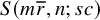$S(m\bar {r}, n; sc)$ as $S_{\infty \,1/s}(m, \pm n; s\sqrt {r}c)$ when $(c, r) = 1$ . After substituting $C \gets s\sqrt {r}C$ , the value of T inside the $\theta $ -factor becomes

$$\begin{align*}\frac{s\sqrt{r} C}{\max(M, q)^{1/2} \max(N, q)^{1/2} \sqrt{Y_MY_N}} \le \frac{s\sqrt{r} C}{rs \sqrt{Y_M Y_N}} = \frac{C}{\sqrt{rY_MY_N}}, \end{align*}$$

and so (5.28) recovers (5.29) up to minor rearrangements.