


1 Introduction
1.1 Overview
Branching graphs – particularly the Young lattice $\mathbb {Y}$
of integer partitions – have long held a central position at the crossroads of representation theory, combinatorics, and probability. Indeed, the Young lattice powers the representation theory of symmetric and (by Schur-Weyl duality) general linear groups, giving rise to Schur functions and driving profound connections to random matrix theory and statistical mechanics. In this landscape, the Plancherel measure on
$\mathbb {Y}$
of integer partitions – have long held a central position at the crossroads of representation theory, combinatorics, and probability. Indeed, the Young lattice powers the representation theory of symmetric and (by Schur-Weyl duality) general linear groups, giving rise to Schur functions and driving profound connections to random matrix theory and statistical mechanics. In this landscape, the Plancherel measure on $\mathbb {Y}$
and its generalization, the Schur measures, have emerged as foundational objects. These probability measures (in the terminology of statistical mechanics, ensembles of random partitions) serve as a framework for exploring phenomena such as limit shapes, random tilings, and universal distributions governing eigenvalues in random matrix ensembles.
$\mathbb {Y}$
and its generalization, the Schur measures, have emerged as foundational objects. These probability measures (in the terminology of statistical mechanics, ensembles of random partitions) serve as a framework for exploring phenomena such as limit shapes, random tilings, and universal distributions governing eigenvalues in random matrix ensembles.
Despite the prominence of the Young lattice, kindred combinatorial structures remain relatively underexplored from a probabilistic perspective. One notable example is the Young–Fibonacci lattice $\mathbb {YF}$
[Reference Fomin33], [Reference Stanley67], [Reference Okada54], [Reference Goodman and Kerov40]. Like the Young lattice,
$\mathbb {YF}$
[Reference Fomin33], [Reference Stanley67], [Reference Okada54], [Reference Goodman and Kerov40]. Like the Young lattice, $\mathbb {YF}$
possesses a 1-differential poset structure defined, not on integer partitions, but rather binary words composed of the symbols
$\mathbb {YF}$
possesses a 1-differential poset structure defined, not on integer partitions, but rather binary words composed of the symbols $1$
and
$1$
and $2$
(known as Fibonacci words). As a 1-differential poset,
$2$
(known as Fibonacci words). As a 1-differential poset, $\mathbb {YF}$
carries a Plancherel measure on Fibonacci words. The Young–Fibonacci lattice also mirrors other structures found in the classical Young lattice, such as versions of the Robinson-Schensted (RS) correspondence, multiparameter analogues of Schur functions, and a representation-theoretic framework introduced by Okada [Reference Okada54]. At the same time,
$\mathbb {YF}$
carries a Plancherel measure on Fibonacci words. The Young–Fibonacci lattice also mirrors other structures found in the classical Young lattice, such as versions of the Robinson-Schensted (RS) correspondence, multiparameter analogues of Schur functions, and a representation-theoretic framework introduced by Okada [Reference Okada54]. At the same time, $\mathbb {YF}$
exhibits novel combinatorial and probabilistic behaviors, which are the main focus of the present work.
$\mathbb {YF}$
exhibits novel combinatorial and probabilistic behaviors, which are the main focus of the present work.
Our starting point is the theory of biserial clone Schur functions [Reference Okada54], a family of functions $s_w(\vec {x}\,|\, \vec {y} \hspace {1pt})$
indexed by Fibonacci words
$s_w(\vec {x}\,|\, \vec {y} \hspace {1pt})$
indexed by Fibonacci words $w\in \mathbb {YF}$
and involving two sequences of parameters
$w\in \mathbb {YF}$
and involving two sequences of parameters $\vec {x}= (x_1, x_2, x_3, \ldots )$
and
$\vec {x}= (x_1, x_2, x_3, \ldots )$
and $\vec {y}= (y_1, y_2, y_3, \ldots )$
. Clone Schur functions, first introduced by Okada, parallel the classical Schur functions
$\vec {y}= (y_1, y_2, y_3, \ldots )$
. Clone Schur functions, first introduced by Okada, parallel the classical Schur functions $s_\lambda (\vec z\hspace {1pt})$
,
$s_\lambda (\vec z\hspace {1pt})$
, $\lambda \in \mathbb {Y}$
,
$\lambda \in \mathbb {Y}$
, $\vec z=(z_1, z_2, z_3, \ldots )$
, in several aspects. Both Schur and biserial clone Schur functions branch according to a Pieri rule and, more generally, obey a Littlewood-Richardson rule which reflects the structure of covering relations in the
$\vec z=(z_1, z_2, z_3, \ldots )$
, in several aspects. Both Schur and biserial clone Schur functions branch according to a Pieri rule and, more generally, obey a Littlewood-Richardson rule which reflects the structure of covering relations in the $\Bbb {Y}$
and
$\Bbb {Y}$
and $\Bbb {YF}$
lattices. As a consequence, both Schur and biserial clone Schur functions give rise to harmonic functions on
$\Bbb {YF}$
lattices. As a consequence, both Schur and biserial clone Schur functions give rise to harmonic functions on $\mathbb {Y}$
and
$\mathbb {Y}$
and $\mathbb {YF}$
, defined respectively by
$\mathbb {YF}$
, defined respectively by
 $$\begin{align*}\lambda \mapsto \frac{s_\lambda(\vec{z} \hspace{1pt})}{s_{\scriptscriptstyle \Box}^n(\vec{z} \hspace{1pt})}, \qquad w \mapsto \frac{s_w(\vec{x} \,|\, \vec{y} \hspace{1pt})}{x_1 \cdots x_n}, \end{align*}$$
where n is the rank of $\lambda \in \mathbb {Y}$
or
$\lambda \in \mathbb {Y}$
or $w \in \mathbb {YF}$
. The Plancherel harmonic function (associated with the Plancherel measure) for each lattice arises from a special choice of parameters in Schur and clone Schur functions, respectively.
$w \in \mathbb {YF}$
. The Plancherel harmonic function (associated with the Plancherel measure) for each lattice arises from a special choice of parameters in Schur and clone Schur functions, respectively.
Positive specializations of classical Schur functions (sequences $\vec z$
for which
$\vec z$
for which $s_\lambda (\vec z\hspace {1pt})$
is positive for all
$s_\lambda (\vec z\hspace {1pt})$
is positive for all $\lambda \in \mathbb {Y}$
) are central in the study of the Young lattice. They are related to total positivity [Reference Aissen, Edrei, Schoenberg and Whitney2], [Reference Aissen, Schoenberg and Whitney3], [Reference Edrei24], [Reference Edrei25], characters of the infinite symmetric group [Reference Thoma70], and asymptotic theory of characters of symmetric groups of increasing order [Reference Vershik and Kerov71].
$\lambda \in \mathbb {Y}$
) are central in the study of the Young lattice. They are related to total positivity [Reference Aissen, Edrei, Schoenberg and Whitney2], [Reference Aissen, Schoenberg and Whitney3], [Reference Edrei24], [Reference Edrei25], characters of the infinite symmetric group [Reference Thoma70], and asymptotic theory of characters of symmetric groups of increasing order [Reference Vershik and Kerov71].
One important distinction with the $\mathbb {YF}$
-lattice is that the harmonic functions on
$\mathbb {YF}$
-lattice is that the harmonic functions on $\mathbb {Y}$
associated with positive specializations of classical Schur functions are extremal (this property is also often called ergodic, or minimal). Extremality means that the functions
$\mathbb {Y}$
associated with positive specializations of classical Schur functions are extremal (this property is also often called ergodic, or minimal). Extremality means that the functions $\lambda \mapsto s_\lambda (\vec {z}\hspace {1pt} ) / s_{\scriptscriptstyle \Box }^n(\vec {z}\hspace {1pt})$
cannot be expressed as a nontrivial convex combination of other nonnegative harmonic functions. In contrast, this extremality property does not generally hold for positive harmonic functions arising from specializations of biserial clone Schur functions. One of the initial motivations for our work was to investigate the broad question of how clone harmonic functions on
$\lambda \mapsto s_\lambda (\vec {z}\hspace {1pt} ) / s_{\scriptscriptstyle \Box }^n(\vec {z}\hspace {1pt})$
cannot be expressed as a nontrivial convex combination of other nonnegative harmonic functions. In contrast, this extremality property does not generally hold for positive harmonic functions arising from specializations of biserial clone Schur functions. One of the initial motivations for our work was to investigate the broad question of how clone harmonic functions on $\mathbb {YF}$
decompose into extremal components. The classification of extremal harmonic functions on
$\mathbb {YF}$
decompose into extremal components. The classification of extremal harmonic functions on $\mathbb {YF}$
was established in [Reference Goodman and Kerov40], and results on the boundary of
$\mathbb {YF}$
was established in [Reference Goodman and Kerov40], and results on the boundary of $\mathbb {YF}$
were strengthened in the preprints [Reference Bochkov and Evtushevsky10], [Reference Evtushevsky26].
$\mathbb {YF}$
were strengthened in the preprints [Reference Bochkov and Evtushevsky10], [Reference Evtushevsky26].
Our first goal is to investigate conditions for which a specialization $(\vec {x}, \vec {y} \hspace {1pt})$
is Fibonacci positive – in the sense that the biserial clone Schur functions
$(\vec {x}, \vec {y} \hspace {1pt})$
is Fibonacci positive – in the sense that the biserial clone Schur functions $s_w(\vec {x}\,|\, \vec {y} \hspace {1pt})$
are strictly positive for all Fibonacci words
$s_w(\vec {x}\,|\, \vec {y} \hspace {1pt})$
are strictly positive for all Fibonacci words $w \in \Bbb {YF}$
. Subsequently, we explore probabilistic and combinatorial properties of Fibonacci positive specializations and related ensembles of random Fibonacci words. The present work extends and completes several well-studied classical topics associated with the Young lattice
$w \in \Bbb {YF}$
. Subsequently, we explore probabilistic and combinatorial properties of Fibonacci positive specializations and related ensembles of random Fibonacci words. The present work extends and completes several well-studied classical topics associated with the Young lattice $\mathbb {Y}$
and Schur functions, adapting them to the Young–Fibonacci lattice
$\mathbb {Y}$
and Schur functions, adapting them to the Young–Fibonacci lattice $\mathbb {YF}$
and clone Schur functions. Our four main contributions can be summarized as follows.
$\mathbb {YF}$
and clone Schur functions. Our four main contributions can be summarized as follows.
1. Characterization of Fibonacci positivity. We establish a complete classification of specializations $(\vec {x}, \vec {y} \hspace {1pt})$
for which the clone Schur functions
$(\vec {x}, \vec {y} \hspace {1pt})$
for which the clone Schur functions $s_w(\vec {x}\,|\, \vec {y} \hspace {1pt})$
are positive for all
$s_w(\vec {x}\,|\, \vec {y} \hspace {1pt})$
are positive for all $w\in \mathbb {YF}$
. The concept of Fibonacci positivity strengthens the notion of total positivity of tridiagonal matrices whose subdiagonal consists entirely of 1’s. We identify two classes of Fibonacci positive specializations, of divergent and convergent type.
$w\in \mathbb {YF}$
. The concept of Fibonacci positivity strengthens the notion of total positivity of tridiagonal matrices whose subdiagonal consists entirely of 1’s. We identify two classes of Fibonacci positive specializations, of divergent and convergent type.
2. Stieltjes moment sequences and orthogonal polynomials. The connection to tridiagonal matrices places the Fibonacci positivity problem within the context of the Stieltjes moment problem and Jacobi continued fractions associated to totally positive tridiagonal matrices. We obtain two new combinatorial formulae for the moments of a Borel measure on $[0,\infty )$
in terms of the recursion parameters of the corresponding family of orthogonal polynomials. The first is a general formula that involves noncrossing set partitions, while the second requires a Fibonacci positive specialization of divergent type and is expressed as a sum over all set partitions. The first formula also exhibits a novel splitting of an integer composition into a unique pair of Fibonacci words.
$[0,\infty )$
in terms of the recursion parameters of the corresponding family of orthogonal polynomials. The first is a general formula that involves noncrossing set partitions, while the second requires a Fibonacci positive specialization of divergent type and is expressed as a sum over all set partitions. The first formula also exhibits a novel splitting of an integer composition into a unique pair of Fibonacci words.
For many examples of Fibonacci positive specializations, the Borel measure on $[0,\infty )$
is (after performing a change of variables) the orthogonality measure for a family of orthogonal polynomials from the (q-)Askey scheme [Reference Koekoek and Swarttouw48], including the Charlier, Type-I Al-Salam–Carlitz, Al-Salam–Chihara, and q-Charlier polynomials. In the latter two examples, the Fibonacci positivity enforces the atypical condition
$[0,\infty )$
is (after performing a change of variables) the orthogonality measure for a family of orthogonal polynomials from the (q-)Askey scheme [Reference Koekoek and Swarttouw48], including the Charlier, Type-I Al-Salam–Carlitz, Al-Salam–Chihara, and q-Charlier polynomials. In the latter two examples, the Fibonacci positivity enforces the atypical condition $q>1$
on the deformation parameter, in contrast to the usual assumption
$q>1$
on the deformation parameter, in contrast to the usual assumption $|q|<1$
in the q-Askey scheme.
$|q|<1$
in the q-Askey scheme.
3. Asymptotics of random Fibonacci words. We investigate the behavior of random Fibonacci words, (with respect to various Fibonacci positive specializations) in the limit as the word length grows. We find examples when growing random words $w\in \mathbb {YF}_n$
,
$w\in \mathbb {YF}_n$
, $n\to \infty $
, exhibit one of the following three patterns:
$n\to \infty $
, exhibit one of the following three patterns:
-
• $w=1^{r_1}21^{r_2}2\ldots $
, where
$r_i$
scale proportionally to n;
$w=1^{r_1}21^{r_2}2\ldots $
, where
$r_i$
scale proportionally to n; -
•
$w=2^{h_1}12^{h_2}1\ldots $
, where
$h_i$
scale proportionally to n; -
•
$w=1^\infty v$
, that is, the word has a single growing prefix of 1’s, followed by a finite (random) Fibonacci word
$v\in \mathbb {YF}$
.


In the first two cases, the joint scaling limit of either $(r_1,r_2,\ldots )$
or
$(r_1,r_2,\ldots )$
or $(h_1,h_2,\ldots )$
displays a “stick-breaking”-type behavior. More precisely, we extend the result of Gnedin–Kerov [Reference Gnedin and Kerov38] who showed that, in the case of the Plancherel measure on
$(h_1,h_2,\ldots )$
displays a “stick-breaking”-type behavior. More precisely, we extend the result of Gnedin–Kerov [Reference Gnedin and Kerov38] who showed that, in the case of the Plancherel measure on $\mathbb {YF}$
, the sequence
$\mathbb {YF}$
, the sequence $(h_1,h_2,\ldots )$
converges to the GEM distribution with parameter
$(h_1,h_2,\ldots )$
converges to the GEM distribution with parameter $\theta =\frac {1}{2}$
.
$\theta =\frac {1}{2}$
.
The Robinson-Schensted correspondence for the $\Bbb {YF}$
-lattice introduced by [Reference Nzeutchap53] (which we revisit in Section 16), the approach using the Stieltjes moment sequences mentioned above, and the results of [Reference Gnedin and Kerov38] connect four distinguished probability distributions:
$\Bbb {YF}$
-lattice introduced by [Reference Nzeutchap53] (which we revisit in Section 16), the approach using the Stieltjes moment sequences mentioned above, and the results of [Reference Gnedin and Kerov38] connect four distinguished probability distributions:
-
• the uniform measures on permutations of
$\{1,2,\ldots ,n\}$
, -
• the Plancherel measures on
$\mathbb {YF}_n$
determined by the differential poset structure, -
• the Poisson distribution on
$\mathbb {Z}_{\ge 0}$
with parameter
$\rho =1$
, and -
• the stick-breaking GEM scheme powered by the Beta distributions.


We extend and deform all these interrelated distributions. In particular, on the Beta distributions side, we find a new family of dependent stick-breaking schemes.
For random Fibonacci words almost surely behaving as $w=1^\infty v$
(the third pattern mentioned above), we determine the probability law of the random finite suffix
$w=1^\infty v$
(the third pattern mentioned above), we determine the probability law of the random finite suffix $v \in \Bbb {YF}$
in the limit in terms of the parameters
$v \in \Bbb {YF}$
in the limit in terms of the parameters $(\vec {x}, \vec {y} \hspace {1pt})$
of the Fibonacci positive specialization. This distribution on the v’s gives the desired decomposition of the clone harmonic function
$(\vec {x}, \vec {y} \hspace {1pt})$
of the Fibonacci positive specialization. This distribution on the v’s gives the desired decomposition of the clone harmonic function $w\mapsto s_w(\vec {x}\,|\, \vec {y} \hspace {1pt})/(x_1\cdots x_{|w|})$
into the extremal components.
$w\mapsto s_w(\vec {x}\,|\, \vec {y} \hspace {1pt})/(x_1\cdots x_{|w|})$
into the extremal components.
4. Clone Cauchy identities and random permutations. We establish clone Cauchy identities which are summation identities involving clone Schur functions, in parallel to the celebrated Cauchy identities for Schur functions. In the Young–Fibonacci setting, the right-hand side of each Cauchy identity is expressed by a quadridiagonal determinant (and not a product, like for classical Schur functions). We employ clone Cauchy identities to study models of random permutations coming from random Fibonacci words and a Robinson–Schensted correspondence for the $\mathbb {YF}$
-lattice introduced in [Reference Nzeutchap53]. In particular, we compute the moment generating function for the number of two-cycles in a certain ensemble of random involutions, and explore its asymptotic behavior under a specific Fibonacci positive specialization. Other specializations may lead to interesting models of random permutations with pattern avoidance properties.
$\mathbb {YF}$
-lattice introduced in [Reference Nzeutchap53]. In particular, we compute the moment generating function for the number of two-cycles in a certain ensemble of random involutions, and explore its asymptotic behavior under a specific Fibonacci positive specialization. Other specializations may lead to interesting models of random permutations with pattern avoidance properties.
In the remainder of the Introduction, we formulate our main results in more detail. Further discussion of possible extensions and open problems is postponed to the last Section 18.
1.2 Clone Schur functions and Fibonacci positivity
A Fibonacci word w is a binary word composed of the symbols 1 and 2. Its weight $|w|$
is the sum of the symbols. For example,
$|w|$
is the sum of the symbols. For example, $|12112|=7$
. By
$|12112|=7$
. By $\mathbb {YF}_n$
we denote the set of Fibonacci words of weight n. The lattice structure on
$\mathbb {YF}_n$
we denote the set of Fibonacci words of weight n. The lattice structure on $\mathbb {YF}$
is defined through branching (covering) relations
$\mathbb {YF}$
is defined through branching (covering) relations $w \nearrow w'$
on pairs of Fibonacci words, where
$w \nearrow w'$
on pairs of Fibonacci words, where $|w'| = |w| + 1$
. This relation is recursively defined to hold if and only if either
$|w'| = |w| + 1$
. This relation is recursively defined to hold if and only if either $w' = 1w$
, or
$w' = 1w$
, or $w' = 2v$
with
$w' = 2v$
with $v \nearrow w$
. The base case is given by
$v \nearrow w$
. The base case is given by $\varnothing \nearrow 1$
. Let
$\varnothing \nearrow 1$
. Let $\dim (w)$
denote the number of saturated chains
$\dim (w)$
denote the number of saturated chains
 $$ \begin{align*}\varnothing=w_0\nearrow w_1\nearrow \cdots \nearrow w_n=w\end{align*} $$
in the Young–Fibonacci lattice starting at $\varnothing $
and ending at w. See Figure 1 for an illustration of
$\varnothing $
and ending at w. See Figure 1 for an illustration of $\mathbb {YF}$
up to level
$\mathbb {YF}$
up to level $n=5$
. A function
$n=5$
. A function $\varphi $
on
$\varphi $
on $\mathbb {YF}$
is called harmonic if
$\mathbb {YF}$
is called harmonic if
 $$ \begin{align*}\varphi(w)=\sum\limits_{w'\colon w \nearrow w'} \varphi(w')\end{align*} $$
for all $w\in \mathbb {YF}$
.
$w\in \mathbb {YF}$
.
Let $\vec x=(x_1, x_2, x_3, \ldots )$
and
$\vec x=(x_1, x_2, x_3, \ldots )$
and $\vec y=(y_1, y_2, y_3, \ldots )$
be two sequences of parameters. Define the
$\vec y=(y_1, y_2, y_3, \ldots )$
be two sequences of parameters. Define the $\ell \times \ell $
tridiagonal determinants by
$\ell \times \ell $
tridiagonal determinants by

where nonzero elements in all rows in $A_{\ell }$
and all rows in
$A_{\ell }$
and all rows in $B_{\ell -1}$
except for the first one follow the pattern
$B_{\ell -1}$
except for the first one follow the pattern $(1,x_j,y_j)$
. Here and throughout the paper,
$(1,x_j,y_j)$
. Here and throughout the paper, $\vec x+r$
and
$\vec x+r$
and $\vec y+r$
denote the sequences with indices shifted by
$\vec y+r$
denote the sequences with indices shifted by $r \in \Bbb {Z}_{\geq 0}$
.
$r \in \Bbb {Z}_{\geq 0}$
.
The clone Schur function $s_w(\vec {x}\,|\, \vec {y} \hspace {1pt})$
is defined by the following recurrence:
$s_w(\vec {x}\,|\, \vec {y} \hspace {1pt})$
is defined by the following recurrence:

The function

is harmonic on $\mathbb {YF}$
. It is normalized so that
$\mathbb {YF}$
. It is normalized so that $\varphi _{\vec x,\vec y} \hspace {1pt} (\varnothing )=1$
.
$\varphi _{\vec x,\vec y} \hspace {1pt} (\varnothing )=1$
.
Our first main result is a complete characterization of the Fibonacci positive sequences $(\vec {x}, \vec {y} \hspace {1pt})$
for which the clone Schur functions
$(\vec {x}, \vec {y} \hspace {1pt})$
for which the clone Schur functions $s_w(\vec {x}\,|\, \vec {y} \hspace {1pt})$
are positive for all
$s_w(\vec {x}\,|\, \vec {y} \hspace {1pt})$
are positive for all $w\in \mathbb {YF}$
:
$w\in \mathbb {YF}$
:
Theorem 1.1 (Theorem 4.12).
All Fibonacci positive sequences $(\vec x,\vec {y}\hspace {1pt})$
have the form
$(\vec x,\vec {y}\hspace {1pt})$
have the form
 $$ \begin{align*} x_k=c_k\hspace{1pt} (1+t_{k-1}),\qquad y_k=c_k\hspace{1pt} c_{k+1}\hspace{1pt} t_k, \qquad k\ge1, \end{align*} $$
where $\vec c$
is an arbitrary positive sequence, and
$\vec c$
is an arbitrary positive sequence, and $\vec t=(t_1,t_2,\ldots )$
(with
$\vec t=(t_1,t_2,\ldots )$
(with $t_0=0$
, for convenience) is a positive real sequence of one of the two types:
$t_0=0$
, for convenience) is a positive real sequence of one of the two types:
-
• (divergent type) The infinite series
(1.1)
$$ \begin{align} 1+t_1+t_1t_2+t_1t_2t_3+\ldots \end{align} $$
diverges, and
$t_{m+1}\ge 1+t_m$
for all
$m\ge 1$
; -
• (convergent type) The series (1.1) converges, and
$$ \begin{align*} 1+t_{m+3}+t_{m+3}t_{m+4}+ t_{m+3}t_{m+4}t_{m+5}+\ldots \ge \frac{t_{m+1}}{t_{m+2}(1+t_m-t_{m+1})} , \qquad \text{for all } m\ge0. \end{align*} $$


The sequences $\vec c$
and
$\vec c$
and $\vec t$
are determined by
$\vec t$
are determined by $(\vec x,\vec {y}\hspace {1pt})$
uniquely.
$(\vec x,\vec {y}\hspace {1pt})$
uniquely.
The distinguished Plancherel harmonic function
 $$ \begin{align*} \varphi_{{}_{\mathrm{PL}}}(w)= \frac{\dim (w)}{n!},\qquad w\in \mathbb{YF}_n, \end{align*} $$
is obtained from clone Schur functions by setting $x_k=y_k=k$
,
$x_k=y_k=k$
, $k\ge 1$
. Throughout the paper we are primarily concerned with two deformations of the Plancherel specialization, of convergent and divergent type, respectively: the shifted Plancherel specialization
$k\ge 1$
. Throughout the paper we are primarily concerned with two deformations of the Plancherel specialization, of convergent and divergent type, respectively: the shifted Plancherel specialization $x_k=y_k=k+\sigma -1$
,
$x_k=y_k=k+\sigma -1$
, $\sigma \in [1,\infty )$
, and the Charlier specialization
$\sigma \in [1,\infty )$
, and the Charlier specialization $x_k=k+\rho -1$
,
$x_k=k+\rho -1$
, $y_k=k\rho $
,
$y_k=k\rho $
, $\rho \in (0,1]$
. In Section 6, we describe other examples of Fibonacci positive specializations, both of divergent and convergent type.
$\rho \in (0,1]$
. In Section 6, we describe other examples of Fibonacci positive specializations, both of divergent and convergent type.
1.3 Stieltjes moment sequences and orthogonal polynomials
As a corollary of the Fibonacci positivity of a specialization $(\vec {x}, \vec {y} \hspace {1pt})$
, we see that the infinite tridiagonal matrix with the diagonals
$(\vec {x}, \vec {y} \hspace {1pt})$
, we see that the infinite tridiagonal matrix with the diagonals $(1,1,\ldots )$
,
$(1,1,\ldots )$
, $(x_1,x_2,\ldots )$
, and
$(x_1,x_2,\ldots )$
, and $(y_1,y_2,\ldots )$
is totally positive, that is, all its minors which are not identically zero are positive. It is known from [Reference Flajolet28], [Reference Viennot72], [Reference Sokal65], [Reference Pétréolle, Sokal and Zhu59] that totally positive tridiagonal matrices correspond to Stieltjes moment sequences
$(y_1,y_2,\ldots )$
is totally positive, that is, all its minors which are not identically zero are positive. It is known from [Reference Flajolet28], [Reference Viennot72], [Reference Sokal65], [Reference Pétréolle, Sokal and Zhu59] that totally positive tridiagonal matrices correspond to Stieltjes moment sequences $a_n=\int t^n {\unicode{x3bd}} (dt)$
,
$a_n=\int t^n {\unicode{x3bd}} (dt)$
, $n\ge 0$
, where
$n\ge 0$
, where ${\unicode{x3bd}} $
is a Borel measure on
${\unicode{x3bd}} $
is a Borel measure on $[0,\infty )$
. Moreover, the monic polynomials
$[0,\infty )$
. Moreover, the monic polynomials $P_n(t)$
,
$P_n(t)$
, $n\ge 0$
, orthogonal with respect to
$n\ge 0$
, orthogonal with respect to ${\unicode{x3bd}} $
can be determined directly in terms of the parameters
${\unicode{x3bd}} $
can be determined directly in terms of the parameters $(\vec {x}, \vec {y} \hspace {1pt})$
:
$(\vec {x}, \vec {y} \hspace {1pt})$
:
 $$ \begin{align*} P_{n+1}(t) = (t - x_{n+1})P_n(t) - y_n P_{n-1}(t), \quad n \geq 1, \qquad P_0(t) = 1, \quad P_1(t) = t - x_1. \end{align*} $$
We refer to Section 7 for a detailed discussion of the connection between total positivity of tridiagonal matrices and Stieltjes moment sequences.
According to the (q-)Askey nomenclature [Reference Koekoek and Swarttouw48], in Section 10 we find several Fibonacci positive specializations whose orthogonal polynomials are (up to a change of variables and parameters):
-
• Charlier polynomials;
-
• Type-I Al-Salam–Carlitz polynomials;
-
• Al-Salam–Chihara polynomials;
-
• q-Charlier polynomials.
In these cases, we also explicitly determine the orthogonality measures $\unicode{x3bd} $
. For example, in the Charlier case, the orthogonality measure is simply the Poisson distribution with the parameter
$\unicode{x3bd} $
. For example, in the Charlier case, the orthogonality measure is simply the Poisson distribution with the parameter $\rho $
. For the Al-Salam–Chihara and q-Charlier polynomials, the Fibonacci positivity enforces the atypical condition
$\rho $
. For the Al-Salam–Chihara and q-Charlier polynomials, the Fibonacci positivity enforces the atypical condition $q>1$
, in contrast to the usual assumption
$q>1$
, in contrast to the usual assumption $|q|<1$
in the q-Askey scheme.
$|q|<1$
in the q-Askey scheme.
The shifted Plancherel specialization $x_k=y_k=k+\sigma -1$
which we consider in Section 11 corresponds to the so-called associated Charlier polynomials [Reference Ismail, Letessier and Valent42], [Reference Ahbli1]. The orthogonality measure
$x_k=y_k=k+\sigma -1$
which we consider in Section 11 corresponds to the so-called associated Charlier polynomials [Reference Ismail, Letessier and Valent42], [Reference Ahbli1]. The orthogonality measure $\unicode{x3bd} $
in this case is not explicit, but we find its moment generating function (Proposition 11.4). Notably, all orthogonality measures
$\unicode{x3bd} $
in this case is not explicit, but we find its moment generating function (Proposition 11.4). Notably, all orthogonality measures $\unicode{x3bd} $
related to known orthogonal polynomials turn out to be discrete. However, not all orthogonal polynomial families with discrete measures correspond to Fibonacci positive specializations (for example, Meixner polynomials do not). An open question is whether there exists a family of orthogonal polynomials with a continuous measure that is Fibonacci positive.
$\unicode{x3bd} $
related to known orthogonal polynomials turn out to be discrete. However, not all orthogonal polynomial families with discrete measures correspond to Fibonacci positive specializations (for example, Meixner polynomials do not). An open question is whether there exists a family of orthogonal polynomials with a continuous measure that is Fibonacci positive.
We also find combinatorial interpretations of the Stieltjes moments $a_n$
associated with Fibonacci positive specializations. There is a rich literature addressing the combinatorics of moments coming from orthogonal polynomials, notably [Reference Wachs and White73], [Reference Zeng74], [Reference Anshelevich4], [Reference Kim, Stanton and Zeng47], [Reference Kasraoui and Zeng46], [Reference Josuat-Vergès and Rubey44], [Reference Corteel, Kim and Stanton20]. Most of the results in Sections 8, 9, and 11 follow from techniques developed in these references. In the case of the Charlier specialization,
$a_n$
associated with Fibonacci positive specializations. There is a rich literature addressing the combinatorics of moments coming from orthogonal polynomials, notably [Reference Wachs and White73], [Reference Zeng74], [Reference Anshelevich4], [Reference Kim, Stanton and Zeng47], [Reference Kasraoui and Zeng46], [Reference Josuat-Vergès and Rubey44], [Reference Corteel, Kim and Stanton20]. Most of the results in Sections 8, 9, and 11 follow from techniques developed in these references. In the case of the Charlier specialization, $a_n$
is the Bell polynomial in the parameter
$a_n$
is the Bell polynomial in the parameter $\rho $
(often called the Touchard polynomial)
$\rho $
(often called the Touchard polynomial)
where the sum is over all set partitions $\pi $
of
$\pi $
of $\{1, \dots , n\}$
. This example is representative of the general behavior of Stieltjes moments arising from Fibonacci positive specializations of divergent type. We prove the following:
$\{1, \dots , n\}$
. This example is representative of the general behavior of Stieltjes moments arising from Fibonacci positive specializations of divergent type. We prove the following:
Proposition 1.2 (Proposition 9.1).
Let $(\vec {x}, \vec {y} \hspace {1pt} )$
be a Fibonacci positive specialization of divergent type
$(\vec {x}, \vec {y} \hspace {1pt} )$
be a Fibonacci positive specialization of divergent type
 $$ \begin{align} x_k=c_k\hspace{1pt} (k +\epsilon_1 + \cdots + \epsilon_{k-1}),\qquad y_k=c_k\hspace{1pt} c_{k+1}\hspace{1pt} (k + \epsilon_1 + \cdots + \epsilon_k), \qquad k\ge1, \end{align} $$
where $\vec {c}$
and
$\vec {c}$
and $\vec {\epsilon }$
are sequences of positive real numbers uniquely determined by (4.7) and Corollary 4.9. Then the associated n-th Stieltjes moment is given by
$\vec {\epsilon }$
are sequences of positive real numbers uniquely determined by (4.7) and Corollary 4.9. Then the associated n-th Stieltjes moment is given by
 $$ \begin{align*} a_n = \sum_{\pi \hspace{1pt} \in \hspace{1pt} \Pi(n)} \, \prod_{k \hspace{1pt} \geq \hspace{1pt} 1} \, c_k^{\hspace{1pt} \ell_{k-1}(\pi)} \hspace{1pt} (1 + \epsilon_k)^{\hspace{1pt} g_k(\pi)}. \end{align*} $$
As in the Charlier case, the sum is taken over all set partitions $\pi \in \Pi (n)$
. The statistics
$\pi \in \Pi (n)$
. The statistics $\ell _k(\pi )$
and
$\ell _k(\pi )$
and $g_k(\pi )$
are defined in Equation (8.1) and are standard in the analysis of set partitions. Although the shifted-Charlier specialization is Fibonacci positive of convergent type (and not divergent type), its Stieltjes moments nevertheless obey a similar expansion formula involving all set partitions; see Proposition 11.7.
$g_k(\pi )$
are defined in Equation (8.1) and are standard in the analysis of set partitions. Although the shifted-Charlier specialization is Fibonacci positive of convergent type (and not divergent type), its Stieltjes moments nevertheless obey a similar expansion formula involving all set partitions; see Proposition 11.7.
Proposition 8.8 presents an expansion formula for the moments $a_n$
of a general Borel measure on
$a_n$
of a general Borel measure on $[0, \infty )$
involving noncrossing set partitions; this result does not require Fibonacci positivity as an assumption. Corollary 8.20 is a compressed version of Proposition 8.8 where
$[0, \infty )$
involving noncrossing set partitions; this result does not require Fibonacci positivity as an assumption. Corollary 8.20 is a compressed version of Proposition 8.8 where $a_n$
is expressed instead as a sum of monomials indexed by integer compositions of n. This result exhibits an intriguing splitting which can be applied to an integer composition to obtain a unique pair of Fibonacci words; see Definition 8.12.
$a_n$
is expressed instead as a sum of monomials indexed by integer compositions of n. This result exhibits an intriguing splitting which can be applied to an integer composition to obtain a unique pair of Fibonacci words; see Definition 8.12.
While we have a complete description of Fibonacci positive specializations $(\vec {x}, \vec {y})$
and an understanding of their corresponding moment sequences
$(\vec {x}, \vec {y})$
and an understanding of their corresponding moment sequences $a_n$
(at least in the divergent case), characterizing their associated Borel measures
$a_n$
(at least in the divergent case), characterizing their associated Borel measures $\unicode{x3bd} $
within the space of all Borel measures on
$\unicode{x3bd} $
within the space of all Borel measures on $[0,\infty )$
remains an open problem.
$[0,\infty )$
remains an open problem.
1.4 Asymptotics of random Fibonacci words
We investigate asymptotic behavior of growing random Fibonacci words distributed according to clone coherent probability measures $M_n$
on
$M_n$
on $\mathbb {YF}_n$
:
$\mathbb {YF}_n$
:
The measures $M_n$
are called coherent since they are compatible for varying n; see (2.5).
$M_n$
are called coherent since they are compatible for varying n; see (2.5).
In Sections 13 and 14, we prove two limit theorems concerning the asymptotic behavior of random Fibonacci words under the Charlier and the shifted Plancherel specializations. For the Charlier specialization $x_k = k + \rho - 1$
,
$x_k = k + \rho - 1$
, $y_k = k\rho $
(which is of divergent type), we decompose the random word as
$y_k = k\rho $
(which is of divergent type), we decompose the random word as $w=1^{r_1}21^{r_2}2\ldots $
.
$w=1^{r_1}21^{r_2}2\ldots $
.
Theorem 1.3 (Theorem 13.2).
Fix $\rho \in (0,1)$
. Let
$\rho \in (0,1)$
. Let $w\in \mathbb {YF}_n$
be distributed according to the Charlier clone coherent measure
$w\in \mathbb {YF}_n$
be distributed according to the Charlier clone coherent measure $M_n$
. Then for each fixed
$M_n$
. Then for each fixed $k\ge 1$
, the joint distribution of runs
$k\ge 1$
, the joint distribution of runs $(r_1(w),\ldots ,r_k(w))$
converges to
$(r_1(w),\ldots ,r_k(w))$
converges to
 $$\begin{align*}\frac{r_j(w)}{n - \sum_{i=1}^{j-1}r_i(w)} \xrightarrow[n\to\infty]{d}\eta_{\rho;j}, \qquad j=1,\dots,k, \end{align*}$$
where $\eta _{\rho ;1}, \eta _{\rho ;2}, \dots $
are i.i.d. copies of a random variable with the distribution
$\eta _{\rho ;1}, \eta _{\rho ;2}, \dots $
are i.i.d. copies of a random variable with the distribution
 $$ \begin{align*} \rho \hspace{1pt}\delta_0(\alpha) + (1 - \rho)\hspace{1pt} \rho (1 - \alpha)^{\rho - 1} \hspace{1pt} d\alpha,\qquad \alpha\in[0,1]. \end{align*} $$
This distribution is a convex combination of the point mass at 0 and the Beta random variable $\mathrm {beta}(1, \rho )$
, with weights
$\mathrm {beta}(1, \rho )$
, with weights $\rho $
and
$\rho $
and $1 - \rho $
.
$1 - \rho $
.
Equivalently, we have $\{r_j/n\}_{j\ge 1}\to X_j$
, where
$\{r_j/n\}_{j\ge 1}\to X_j$
, where $X_1=U_1$
and
$X_1=U_1$
and $X_n=(1-U_1)\cdots (1-U_{n-1})U_n$
for
$X_n=(1-U_1)\cdots (1-U_{n-1})U_n$
for $n\ge 2$
, where
$n\ge 2$
, where $U_j=\eta _{\rho ;j}$
are i.i.d. The representation of the vector
$U_j=\eta _{\rho ;j}$
are i.i.d. The representation of the vector $(X_1,X_2,\ldots )$
through the variables
$(X_1,X_2,\ldots )$
through the variables $U_j$
is called a stick-breaking process.
$U_j$
is called a stick-breaking process.
Note that if $U_j$
have the distribution
$U_j$
have the distribution $\mathrm {beta}(1, \theta )$
, then the distribution of the vector
$\mathrm {beta}(1, \theta )$
, then the distribution of the vector $(X_1,X_2,\ldots )$
is called the Griffiths–Engen–McCloskey distribution
$(X_1,X_2,\ldots )$
is called the Griffiths–Engen–McCloskey distribution $\mathrm {GEM}(\theta )$
. We refer to [Reference Johnson, Kotz and Balakrishnan43, Chapter 41] for further discussion and applications of GEM distributions, in particular, in population genetics.
$\mathrm {GEM}(\theta )$
. We refer to [Reference Johnson, Kotz and Balakrishnan43, Chapter 41] for further discussion and applications of GEM distributions, in particular, in population genetics.
We see that the runs of $1$
’s under the Charlier specialization scale to the
$1$
’s under the Charlier specialization scale to the $\mathrm {GEM}(\rho )$
vector with additional zero entries inserted independently with density
$\mathrm {GEM}(\rho )$
vector with additional zero entries inserted independently with density $1-\rho $
.
$1-\rho $
.
For the shifted Plancherel specialization $x_k=y_k=k+\sigma -1$
(which is of convergent type), we decompose the random word as
$x_k=y_k=k+\sigma -1$
(which is of convergent type), we decompose the random word as $w=2^{h_1}12^{h_2}1\ldots $
. Denote
$w=2^{h_1}12^{h_2}1\ldots $
. Denote $\tilde h_j=2h_j+1$
.
$\tilde h_j=2h_j+1$
.
Theorem 1.4 (Theorem 14.4).
Fix $\sigma \ge 1$
. Under the shifted Plancherel clone coherent measure
$\sigma \ge 1$
. Under the shifted Plancherel clone coherent measure $M_n$
, we have for the joint distribution
$M_n$
, we have for the joint distribution $(\tilde h_1(w),\ldots ,\tilde h_k(w))$
for each fixed
$(\tilde h_1(w),\ldots ,\tilde h_k(w))$
for each fixed $k\ge 1$
:
$k\ge 1$
:
 $$ \begin{align*} \frac{\tilde h_j(w)}{n-\sum_{i=1}^{j-1}\tilde h_i(w)}\xrightarrow[n\to\infty]{d}\xi_{\sigma;j},\qquad j=1,\ldots,k. \end{align*} $$
The joint distribution of $(\xi _{\sigma ;1},\xi _{\sigma ;2},\ldots )$
can be described as follows. Toss a sequence of independent coins with probabilities of success
$(\xi _{\sigma ;1},\xi _{\sigma ;2},\ldots )$
can be described as follows. Toss a sequence of independent coins with probabilities of success $1,\sigma ^{-1},\sigma ^{-2},\ldots $
. Let N be the (random) number of successes until the first failure. Then, sample N independent
$1,\sigma ^{-1},\sigma ^{-2},\ldots $
. Let N be the (random) number of successes until the first failure. Then, sample N independent $\mathrm {beta}(1,\sigma /2)$
random variables. Set
$\mathrm {beta}(1,\sigma /2)$
random variables. Set $\xi _{\sigma ;k}$
,
$\xi _{\sigma ;k}$
, $k=1,\ldots ,N $
, to be these random variables, while
$k=1,\ldots ,N $
, to be these random variables, while $\xi _{\sigma ;k}=0$
for
$\xi _{\sigma ;k}=0$
for $k>N$
.
$k>N$
.
When $\sigma>1$
, the random variables
$\sigma>1$
, the random variables $\xi _{\sigma ;k}$
are not independent, but
$\xi _{\sigma ;k}$
are not independent, but $\xi _{\sigma ;1},\ldots ,\xi _{\sigma ;n} $
are conditionally independent given
$\xi _{\sigma ;1},\ldots ,\xi _{\sigma ;n} $
are conditionally independent given $N=n$
. Almost surely, the sequence
$N=n$
. Almost surely, the sequence $\xi _{\sigma ;1},\xi _{\sigma ;2},\ldots $
contains only finitely many nonzero terms.
$\xi _{\sigma ;1},\xi _{\sigma ;2},\ldots $
contains only finitely many nonzero terms.
At $\sigma =1$
(Plancherel measure), we have
$\sigma =1$
(Plancherel measure), we have $N=\infty $
almost surely, so the random variables
$N=\infty $
almost surely, so the random variables $\xi _{1;k}$
are i.i.d.
$\xi _{1;k}$
are i.i.d. $\mathrm {beta}(1,\sigma /2)$
. Thus, we recover the convergence to GEM
$\mathrm {beta}(1,\sigma /2)$
. Thus, we recover the convergence to GEM $(1/2)$
obtained in [Reference Gnedin and Kerov38].
$(1/2)$
obtained in [Reference Gnedin and Kerov38].
Theorems 1.3 and 1.4 follow from product-like formulas for the joint distributions of $r_j(w)$
and
$r_j(w)$
and $h_j(w)$
, respectively. The product-like formulas are valid for arbitrary Fibonacci positive specializations, but they greatly simplify in the Charlier and shifted Plancherel cases.
$h_j(w)$
, respectively. The product-like formulas are valid for arbitrary Fibonacci positive specializations, but they greatly simplify in the Charlier and shifted Plancherel cases.
Consider now generic specializations of convergent type with an additional property that the infinite product $\prod _{i=1}^\infty (1+t_i)$
converges to a finite nonzero value.
$\prod _{i=1}^\infty (1+t_i)$
converges to a finite nonzero value.
Theorem 1.5 (Propositions 15.4 and 15.6).
For a sequence $\vec t$
of convergent type subject to the assumption above, the behavior of a random word
$\vec t$
of convergent type subject to the assumption above, the behavior of a random word $w\in \mathbb {YF}_n$
, sampled with respect to the corresponding clone coherent measure, in the limit as
$w\in \mathbb {YF}_n$
, sampled with respect to the corresponding clone coherent measure, in the limit as $n\to \infty $
is as follows:
$n\to \infty $
is as follows:
-
• either
$w \to 1^\infty $
-
• or
$w \to 1^\infty 2v$
, where
$v \in \mathbb {YF}$
is a finite random Fibonacci word.


That is, the growing word w stabilizes to a random element of the set
Moreover, the distribution $\mu _{\hspace {0.5pt}\mathrm {I}}$
of the limiting random word
$\mu _{\hspace {0.5pt}\mathrm {I}}$
of the limiting random word $w\in 1^\infty \mathbb {YF}$
is given by
$w\in 1^\infty \mathbb {YF}$
is given by
 $$ \begin{align*} \mu_{\hspace{0.5pt}\mathrm{I}}\left( 1^\infty \right)= \prod_{i=1}^\infty(1+t_i)^{-1}, \qquad \mu_{\hspace{0.5pt}\mathrm{I}}\left( 1^\infty2u \right)= \Bigg( \, \prod_{i \hspace{1pt} = \hspace{1pt} 1}^{|u|-1}(1+t_i) \Bigg) \big(|u|+1 \big)\hspace{1pt} M_{|u|}(u) \hspace{1pt} \frac{B_{\infty}(|u|)}{\prod_{i=1}^{\infty}(1+t_i)}, \end{align*} $$
where $u\in \mathbb {YF}$
is arbitrary, and
$u\in \mathbb {YF}$
is arbitrary, and $B_\infty (m)$
,
$B_\infty (m)$
, $m\ge 0$
, is an infinite series defined below in (4.4). Moreover,
$m\ge 0$
, is an infinite series defined below in (4.4). Moreover, $\mu _{\hspace {0.5pt}\mathrm {I}}$
is a probability measure on
$\mu _{\hspace {0.5pt}\mathrm {I}}$
is a probability measure on $1^\infty \mathbb {YF}$
.
$1^\infty \mathbb {YF}$
.
In Corollary 15.7, we obtain the following decomposition of the clone harmonic function $\varphi _{\vec x, \vec y}$
for specializations of convergent type satisfying
$\varphi _{\vec x, \vec y}$
for specializations of convergent type satisfying $\prod _{i=1}^\infty (1+t_i)<\infty $
:
$\prod _{i=1}^\infty (1+t_i)<\infty $
:

Here, $\unlhd $
denotes the partial order on
$\unlhd $
denotes the partial order on $\mathbb {YF}$
(induced from the branching relation). The functions
$\mathbb {YF}$
(induced from the branching relation). The functions $\Phi _{1^\infty }$
and
$\Phi _{1^\infty }$
and $\Phi _{1^\infty 2u}$
for
$\Phi _{1^\infty 2u}$
for $v \in \Bbb {YF}$
are called Type-I harmonic functions, and they are extremal.
$v \in \Bbb {YF}$
are called Type-I harmonic functions, and they are extremal.
1.5 Clone Cauchy identities and random permutations
In Section 3, we derive clone Cauchy identities generalizing the classical Cauchy-type summation formulas for the usual Schur functions. Two identities are presented in Propositions 3.8 and 3.9, with the second being
 $$ \begin{align} \sum_{|w| = n} s_w (\vec{p} \,|\, \vec{q}\hspace{1pt}) \hspace{1pt} s_w (\vec{x} \,|\, \vec{y}\hspace{1pt}) = \det \underbrace{\begin{pmatrix} \mathrm{A}_1 & \mathrm{B}_1 & \mathrm{C}_1 & 0 & \cdots \\ 1 & \mathrm{A}_2 & \mathrm{B}_2 & \mathrm{C}_2 & \\ 0 & 1 & \mathrm{A}_3 & \mathrm{B}_3 & \\ 0 & 0 & 1 & \mathrm{A}_4 & \\ \vdots & & & & \ddots \end{pmatrix}}_{n \times n \ \mathrm{quadridiagonal \, matrix}}, \end{align} $$
where $\mathrm {A}_k = p_k x_k$
,
$\mathrm {A}_k = p_k x_k$
, $\mathrm {B}_k = q_k(x_k x_{k+1} - y_k) + y_k(p_k p_{k+1} - q_k)$
,
$\mathrm {B}_k = q_k(x_k x_{k+1} - y_k) + y_k(p_k p_{k+1} - q_k)$
, $\mathrm {C}_k = p_k x_k q_{k+1} y_{k+1}$
.
$\mathrm {C}_k = p_k x_k q_{k+1} y_{k+1}$
.
The identity in (1.3) can be used to define clone analogues of Schur measures, extending the framework from harmonic functions on $\mathbb {YF}$
. Indeed, when one of the specializations in (1.3) is Plancherel,
$\mathbb {YF}$
. Indeed, when one of the specializations in (1.3) is Plancherel, $p_k = q_k = k$
, identity (1.3) reduces to the normalizing identity for the clone harmonic function
$p_k = q_k = k$
, identity (1.3) reduces to the normalizing identity for the clone harmonic function $\varphi _{\vec x, \vec y}$
. For the Young lattice, Schur measures were introduced in [Reference Okounkov55] and generalized to Schur processes (measures on sequences of partitions) in [Reference Okounkov and Reshetikhin57]. They found extensive applications in random matrices, interacting particle systems, random discrete structures like tilings, geometry, and other areas [Reference Okounkov and Pandharipande56], [Reference Okounkov, Reshetikhin, Vafa, Etingof, Retakh and Singer58], [Reference Borodin and Ferrari11], [Reference Borodin and Gorin12], [Reference Borodin and Petrov15], [Reference Corwin and Hammond21]. We leave clone analogues of Schur measures and processes for future work.
$\varphi _{\vec x, \vec y}$
. For the Young lattice, Schur measures were introduced in [Reference Okounkov55] and generalized to Schur processes (measures on sequences of partitions) in [Reference Okounkov and Reshetikhin57]. They found extensive applications in random matrices, interacting particle systems, random discrete structures like tilings, geometry, and other areas [Reference Okounkov and Pandharipande56], [Reference Okounkov, Reshetikhin, Vafa, Etingof, Retakh and Singer58], [Reference Borodin and Ferrari11], [Reference Borodin and Gorin12], [Reference Borodin and Petrov15], [Reference Corwin and Hammond21]. We leave clone analogues of Schur measures and processes for future work.
In Section 16, we introduce ensembles of random permutations and involutions by utilizing the Young–Fibonacci RS correspondence [Reference Nzeutchap53] and positive harmonic functions on $\mathbb {YF}$
. In full generality, the distribution of a permutation or involution depends, respectively, on a triplet
$\mathbb {YF}$
. In full generality, the distribution of a permutation or involution depends, respectively, on a triplet $(\unicode{x3c0} , \varphi , \psi )$
or a couple
$(\unicode{x3c0} , \varphi , \psi )$
or a couple $(\unicode{x3c0} , \varphi )$
of harmonic functions. We do not treat the general case in the present work, but focus on the clone harmonic / Plancherel random involutions, that is, corresponding to setting
$(\unicode{x3c0} , \varphi )$
of harmonic functions. We do not treat the general case in the present work, but focus on the clone harmonic / Plancherel random involutions, that is, corresponding to setting $\unicode{x3c0} = \varphi _{\vec x, \vec y}$
and
$\unicode{x3c0} = \varphi _{\vec x, \vec y}$
and $\varphi = \varphi _{{}_{\mathrm {PL}}}$
, where
$\varphi = \varphi _{{}_{\mathrm {PL}}}$
, where $(\vec x, \vec y)$
is a Fibonacci positive specialization. Using clone Cauchy identities, in Section 17 we find the moment generating function for the number of two-cycles in a random involution
$(\vec x, \vec y)$
is a Fibonacci positive specialization. Using clone Cauchy identities, in Section 17 we find the moment generating function for the number of two-cycles in a random involution $\boldsymbol {\unicode{x3c3}} \in \mathfrak {S}_n$
(Proposition 17.1):
$\boldsymbol {\unicode{x3c3}} \in \mathfrak {S}_n$
(Proposition 17.1):
 $$ \begin{align*} \operatorname{\mathbb{E}}\big[ \tau^{\# \hspace{1pt} \mathrm{two \text{-} cycles}(\boldsymbol{\unicode{x3c3}}) } \big] = (x_1 \cdots x_n)^{-1} \hspace{1pt} \det \underbrace{\begin{pmatrix} x_1 &(1 - \tau ) y_1 & - \tau x_1 y_2 &0 &\cdots \\ 1 &x_2 &(1 - 2 \tau)y_2 &- 2 \tau x_2 y_3 & \\ 0 &1 &x_3 &(1 - 3 \tau )y_3 & \\ 0 &0 &1 &x_4 & \\ \vdots & & & &\ddots \end{pmatrix}}_{n \times n \ \mathrm{quadridiagonal \, matrix}} , \end{align*} $$
where $\tau $
is an auxiliary parameter.
$\tau $
is an auxiliary parameter.
When $(\vec {x}, \vec {y})$
is the shifted Plancherel specialization (
$(\vec {x}, \vec {y})$
is the shifted Plancherel specialization ( $x_k = y_k = k + \sigma - 1$
,
$x_k = y_k = k + \sigma - 1$
, $\sigma \in [1,\infty )$
), the Young–Fibonacci shape
$\sigma \in [1,\infty )$
), the Young–Fibonacci shape $w\in \mathbb {YF}_n$
of a random involution
$w\in \mathbb {YF}_n$
of a random involution $\boldsymbol {\unicode{x3c3}} \in \mathfrak {S}_n$
under the RS correspondence has the same distribution as a random Fibonacci word considered in Theorem 1.4 above. In this way, we can compare the asymptotic behavior of the total number of
$\boldsymbol {\unicode{x3c3}} \in \mathfrak {S}_n$
under the RS correspondence has the same distribution as a random Fibonacci word considered in Theorem 1.4 above. In this way, we can compare the asymptotic behavior of the total number of $2$
’s in a random Fibonacci word (which is the same as the number of two-cycles), and the scaling limit of initial long sequences of
$2$
’s in a random Fibonacci word (which is the same as the number of two-cycles), and the scaling limit of initial long sequences of $2$
’s from Theorem 1.4. We establish a law of large numbers (Proposition 17.6) for the total number of
$2$
’s from Theorem 1.4. We establish a law of large numbers (Proposition 17.6) for the total number of $2$
’s:
$2$
’s:
 $$ \begin{align} \lim_{n\to\infty} \frac{\# \mathrm{two \text{-} cycles}(\boldsymbol{\unicode{x3c3}})}{n} = \frac{1}{\sigma+1}. \end{align} $$
For $\sigma> 1$
, this value exceeds the expectation of the sum of the scaled quantities
$\sigma> 1$
, this value exceeds the expectation of the sum of the scaled quantities $h_j$
in Theorem 1.4. This discrepancy reveals that additional digits of
$h_j$
in Theorem 1.4. This discrepancy reveals that additional digits of $2$
remain hidden in the growing random Fibonacci word after long sequences of
$2$
remain hidden in the growing random Fibonacci word after long sequences of $1$
’s. This behavior is unaccounted for in the scaling limit of Theorem 1.4 but contributes to the law of large numbers (1.4).
$1$
’s. This behavior is unaccounted for in the scaling limit of Theorem 1.4 but contributes to the law of large numbers (1.4).
Outline of the paper
The paper is organized into three parts.
In Part I (Sections 2 to 6), we introduce the Young–Fibonacci lattice, the biserial clone Schur functions, and the associated clone coherent measures. We prove the clone Cauchy summation identities, and give a complete characterization of Fibonacci positive specializations of both divergent and convergent type. Representative examples include the shifted Plancherel and Charlier cases that will serve as running examples in later sections.
In Part II (Sections 7 to 11), we develop the link between Fibonacci positivity, total positivity of tridiagonal matrices, and Stieltjes moment sequences. We obtain general combinatorial formulas for moments, identify families of orthogonal polynomials from the (q-)Askey scheme (Charlier, Type-I Al-Salam–Carlitz, Al-Salam–Chihara, q-Charlier), and highlight the atypical $q>1$
regime enforced by Fibonacci positivity. For these and other specializations, we determine the corresponding discrete Borel orthogonality measures and give explicit combinatorial interpretations of the moments.
$q>1$
regime enforced by Fibonacci positivity. For these and other specializations, we determine the corresponding discrete Borel orthogonality measures and give explicit combinatorial interpretations of the moments.
In Part III (Sections 12 to 17), we study the asymptotic behavior of random Fibonacci words under various Fibonacci positive specializations. Our results include stick-breaking-type limit laws extending the GEM( $\tfrac 12$
) scaling limit of [Reference Gnedin and Kerov38], new dependent stick-breaking schemes, and the description of extremal components in terms of Type-I harmonic functions in the Martin boundary. We further employ clone Cauchy identities to define and analyze models of random permutations and involutions, computing exact generating functions for cycle statistics and establishing laws of large numbers.
$\tfrac 12$
) scaling limit of [Reference Gnedin and Kerov38], new dependent stick-breaking schemes, and the description of extremal components in terms of Type-I harmonic functions in the Martin boundary. We further employ clone Cauchy identities to define and analyze models of random permutations and involutions, computing exact generating functions for cycle statistics and establishing laws of large numbers.
The paper concludes in Section 18 with a discussion of possible extensions and open problems.
Reading guide
Parts II and III are largely independent and can be read in either order after Part I. Readers primarily interested in the asymptotic behavior of random Fibonacci words (like the scaling limit in Theorem 13.2) may proceed directly to Part III after reading Part I, specifically Sections 2, 4 and 6 for the necessary background and definitions.
Part I Young–Fibonacci lattice and Fibonacci positivity
In this part we recall, and when necessary introduce, the principal objects of our study: the Young-Fibonacci lattice $\mathbb {YF}$
, the clone Schur functions, and the clone coherent measures on Fibonacci words. We then characterize those specializations of the clone Schur functions that give rise to positive harmonic functions on
$\mathbb {YF}$
, the clone Schur functions, and the clone coherent measures on Fibonacci words. We then characterize those specializations of the clone Schur functions that give rise to positive harmonic functions on $\mathbb {YF}$
. Finally, we present several examples of Fibonacci positive specializations, including the ones whose asymptotics we analyze in Part III.
$\mathbb {YF}$
. Finally, we present several examples of Fibonacci positive specializations, including the ones whose asymptotics we analyze in Part III.
2 Young–Fibonacci lattice and clone Schur functions
In this preliminary section we review the Young–Fibonacci lattice $\mathbb {YF}$
(also referred to as the Young–Fibonacci branching graph) [Reference Fomin33], [Reference Stanley67], [Reference Goodman and Kerov40] and the clone Schur functions introduced in [Reference Okada54]. The biserial clone Schur functions are harmonic on
$\mathbb {YF}$
(also referred to as the Young–Fibonacci branching graph) [Reference Fomin33], [Reference Stanley67], [Reference Goodman and Kerov40] and the clone Schur functions introduced in [Reference Okada54]. The biserial clone Schur functions are harmonic on $\mathbb {YF}$
, and we use them to define coherent probability measures on Fibonacci words.
$\mathbb {YF}$
, and we use them to define coherent probability measures on Fibonacci words.
2.1 Young–Fibonacci lattice and harmonic functions
A Fibonacci word $w=w_1\ldots w_\ell $
is any binary word with letters
$w=w_1\ldots w_\ell $
is any binary word with letters $w_j\in \left \{ 1,2 \right \}$
. The integer
$w_j\in \left \{ 1,2 \right \}$
. The integer ![]() is called the weight of the word w. The total number of Fibonacci words of weight n is equal to the n-th Fibonacci number,Footnote
1
hence the name. Denote the set of all Fibonacci words of weight n by
is called the weight of the word w. The total number of Fibonacci words of weight n is equal to the n-th Fibonacci number,Footnote
1
hence the name. Denote the set of all Fibonacci words of weight n by $\mathbb {YF}_{n}$
, where
$\mathbb {YF}_{n}$
, where $n\ge 0$
.
$n\ge 0$
.
Definition 2.1. The Young–Fibonacci lattice $\mathbb {YF}$
is the union of all sets
$\mathbb {YF}$
is the union of all sets $\mathbb {YF}_{n}$
,
$\mathbb {YF}_{n}$
, $n\ge 0$
. In this lattice,
$n\ge 0$
. In this lattice, $w\in \mathbb {YF}_n$
is connected to
$w\in \mathbb {YF}_n$
is connected to $w'\in \mathbb {YF}_{n+1}$
if and only if
$w'\in \mathbb {YF}_{n+1}$
if and only if $w'$
can be obtained from w by one of the following three operations:
$w'$
can be obtained from w by one of the following three operations:
-
F1.
$w'=1w$
. -
F1.
$w'=2^{k+1}v$
if
$w=2^k1v$
for some
$k\ge 0$
and an arbitrary Fibonacci word v. -
F1.
$w'=2^\ell 1 2^{k-\ell }v$
if
$w=2^kv$
for some
$k\ge 1$
and an arbitrary Fibonacci word v. While F1 and F2 each generate at most one edge, this rule generates k edges indexed by
$\ell =1,\ldots ,k$
.


We denote this relation by $w\nearrow w'$
(equivalently,
$w\nearrow w'$
(equivalently, $w'\searrow w$
). An example of the Young–Fibonacci lattice up to level
$w'\searrow w$
). An example of the Young–Fibonacci lattice up to level $n=5$
is given in Figure 1.
$n=5$
is given in Figure 1.
The Young–Fibonacci lattice up to level $n=5$
.
$n=5$
.

Definition 2.2. A function $\varphi $
on
$\varphi $
on $\mathbb {YF}$
is called harmonic if it satisfies
$\mathbb {YF}$
is called harmonic if it satisfies
 $$ \begin{align*} \varphi(w)=\sum_{w'\colon w' \searrow w} \varphi(w')\qquad \text{for all } w\in \mathbb{YF}. \end{align*} $$
A harmonic function is called normalized if $\varphi (\varnothing )=1$
.
$\varphi (\varnothing )=1$
.
For $w\in \mathbb {YF}$
, denote by
$w\in \mathbb {YF}$
, denote by $\dim (w)$
the number of oriented paths (also known as saturated chains) from
$\dim (w)$
the number of oriented paths (also known as saturated chains) from $\varnothing $
to w in the Young–Fibonacci lattice. Let
$\varnothing $
to w in the Young–Fibonacci lattice. Let $I_2(w)$
be the sequence of all positions of the letter 2 in w, reading from left to right. Then
$I_2(w)$
be the sequence of all positions of the letter 2 in w, reading from left to right. Then
 $$ \begin{align} \dim(w) =\prod_{i\in I_2(w)} \mathsf{d}_i(w),\quad \text{where } \mathsf{d}_i(w)=|v|+1 \text{ if } w=u2v \text{ is the splitting of } w \text{ at position } i. \end{align} $$
Equivalently, $\dim (w)$
obeys the following recursion:
$\dim (w)$
obeys the following recursion:
 $$ \begin{align} \dim(w) \, = \, \begin{cases} 1, & \text{if } w = \varnothing ;\\ \dim(v), & \text{if } w = 1v \text{ for a Fibonacci word } v ;\\ (|v| + 1) \dim(v), & \text{if } w = 2v \text{ for a Fibonacci word } v. \end{cases} \end{align} $$
For example, if $w=22121$
, then
$w=22121$
, then $I_2(w)=( 1,2,4 )$
, and
$I_2(w)=( 1,2,4 )$
, and $\dim w=70$
. Since
$\dim w=70$
. Since $\mathbb {YF}$
is a
$\mathbb {YF}$
is a $1$
-differential poset, we have [Reference Stanley67, Corollary 3.9], (see also [Reference Fomin29]):
$1$
-differential poset, we have [Reference Stanley67, Corollary 3.9], (see also [Reference Fomin29]):
 $$ \begin{align} \sum_{w\in \mathbb{YF}_n} \dim^2 (w) = n!\hspace{1pt}. \end{align} $$
With any nonnegative normalized harmonic function we can associate a family of probability measures $M_n$
on
$M_n$
on $\mathbb {YF}_n$
as follows:
$\mathbb {YF}_n$
as follows:
The fact that $\sum _{w\in \mathbb {YF}_n} M_n(w)=1$
follows from the normalization of
$\sum _{w\in \mathbb {YF}_n} M_n(w)=1$
follows from the normalization of $\varphi $
, and the harmonicity of
$\varphi $
, and the harmonicity of $\varphi $
translates into the coherence property of the measures
$\varphi $
translates into the coherence property of the measures $M_n$
:
$M_n$
:
 $$ \begin{align} M_n(w)=\sum_{w'\colon w'\searrow w} M_{n+1}(w')\hspace{1pt} \frac{\dim (w)}{\dim (w')}, \qquad w\in \mathbb{YF}_n. \end{align} $$
The set of all nonnegative normalized harmonic functions on $\mathbb {YF}$
forms a simplex
$\mathbb {YF}$
forms a simplex $\Upsilon (\mathbb {YF})$
. The set of extreme points of this simplex (the ones not expressible as a nontrivial convex combination of other points) is denoted by
$\Upsilon (\mathbb {YF})$
. The set of extreme points of this simplex (the ones not expressible as a nontrivial convex combination of other points) is denoted by $\Upsilon _{\mathrm {ext}}(\mathbb {YF})$
. In general,
$\Upsilon _{\mathrm {ext}}(\mathbb {YF})$
. In general, $\Upsilon _{\mathrm {ext}}(\mathbb {YF})$
is a subset of the Martin boundary, denoted by
$\Upsilon _{\mathrm {ext}}(\mathbb {YF})$
is a subset of the Martin boundary, denoted by $\Upsilon _{\mathrm {Martin}}(\mathbb {YF})$
. The latter consists of harmonic functions which can be obtained by finite rank approximation. The Martin boundary of the Young–Fibonacci lattice is described in [Reference Goodman and Kerov40]. Recently, it was shown in the preprints [Reference Bochkov and Evtushevsky10], [Reference Evtushevsky26] that the Martin boundary coincides with the set of extreme points
$\Upsilon _{\mathrm {Martin}}(\mathbb {YF})$
. The latter consists of harmonic functions which can be obtained by finite rank approximation. The Martin boundary of the Young–Fibonacci lattice is described in [Reference Goodman and Kerov40]. Recently, it was shown in the preprints [Reference Bochkov and Evtushevsky10], [Reference Evtushevsky26] that the Martin boundary coincides with the set of extreme points $\Upsilon _{\mathrm {ext}}(\mathbb {YF})$
.
$\Upsilon _{\mathrm {ext}}(\mathbb {YF})$
.
For any coherent family of measures $M_n$
on
$M_n$
on $\mathbb {YF}_n$
,
$\mathbb {YF}_n$
, $n=0,1,2,\ldots $
, there exists a unique probability measure
$n=0,1,2,\ldots $
, there exists a unique probability measure $\mu $
on
$\mu $
on $\Upsilon _{\mathrm {ext}}(\mathbb {YF})$
such that
$\Upsilon _{\mathrm {ext}}(\mathbb {YF})$
such that
 $$ \begin{align} M_n(w)=\int_{\Upsilon_{\mathrm{ext}}(\mathbb{YF})} \dim(w)\hspace{1pt} \varphi_\omega(w)\hspace{1pt} \mu(d\hspace{1pt} \omega),\qquad w\in \mathbb{YF}_n. \end{align} $$
Here $\varphi _\omega $
is the extremal harmonic function corresponding to
$\varphi _\omega $
is the extremal harmonic function corresponding to $\omega \in \Upsilon _{\mathrm {ext}}(\mathbb {YF})$
.
$\omega \in \Upsilon _{\mathrm {ext}}(\mathbb {YF})$
.
2.2 Plancherel measure and its scaling limit
An important example of a harmonic function on $\mathbb {YF}$
is the Plancherel function defined as
$\mathbb {YF}$
is the Plancherel function defined as
In [Reference Gnedin and Kerov38] it is shown that $\varphi _{{}_{\mathrm {PL}}}$
belongs to
$\varphi _{{}_{\mathrm {PL}}}$
belongs to $\Upsilon _{\mathrm {ext}}(\mathbb {YF})$
. Moreover, for the Plancherel measure
$\Upsilon _{\mathrm {ext}}(\mathbb {YF})$
. Moreover, for the Plancherel measure $M_n(w)=\dim ^2 (w)/n!$
corresponding to
$M_n(w)=\dim ^2 (w)/n!$
corresponding to $\varphi _{{}_{\mathrm {PL}}}$
as in (2.4), [Reference Gnedin and Kerov38] establishes a
$\varphi _{{}_{\mathrm {PL}}}$
as in (2.4), [Reference Gnedin and Kerov38] establishes a $n\to \infty $
scaling limit theorem for the positions of the
$n\to \infty $
scaling limit theorem for the positions of the $1$
’s in the random Fibonacci word w which we now describe.
$1$
’s in the random Fibonacci word w which we now describe.
Represent $w\in \mathbb {YF}$
as a sequence of contiguous blocks of letters 2 separated by 1’s. For example,
$w\in \mathbb {YF}$
as a sequence of contiguous blocks of letters 2 separated by 1’s. For example, $w=122112=(1)(221)(1)(2)$
. Each block except possibly the rightmost one contains exactly one 1, which is its terminating letter. Denote by
$w=122112=(1)(221)(1)(2)$
. Each block except possibly the rightmost one contains exactly one 1, which is its terminating letter. Denote by $\tilde {h}_1, \tilde {h}_2, \ldots $
the sequence of weights of the blocks, reading from left to right. For the example above,
$\tilde {h}_1, \tilde {h}_2, \ldots $
the sequence of weights of the blocks, reading from left to right. For the example above, $\tilde {h}_1=1, \tilde {h}_2=5, \tilde {h}_3=1, \tilde {h}_4=2$
, and
$\tilde {h}_1=1, \tilde {h}_2=5, \tilde {h}_3=1, \tilde {h}_4=2$
, and $\tilde {h}_j=0$
for
$\tilde {h}_j=0$
for $j\ge 5$
. We have
$j\ge 5$
. We have $\tilde {h}_1+\tilde {h}_2+\ldots =n$
.
$\tilde {h}_1+\tilde {h}_2+\ldots =n$
.
Definition 2.3. The GEM (Griffiths–Engen–McCloskey) distribution with parameter $\theta>0$
(denoted
$\theta>0$
(denoted $\mathrm {GEM}(\theta )$
) is a probability measure on the infinite-dimensional simplex
$\mathrm {GEM}(\theta )$
) is a probability measure on the infinite-dimensional simplex

obtained from the residual allocation model (also called the stick-breaking construction) as follows. By definition, a random point $X=(X_1,X_2,\ldots )\in \Delta $
under
$X=(X_1,X_2,\ldots )\in \Delta $
under $\mathrm {GEM}(\theta )$
is distributed as
$\mathrm {GEM}(\theta )$
is distributed as
 $$ \begin{align*} X_1=U_1,\qquad X_n=(1-U_1)(1-U_2)\cdots(1-U_{n-1})U_n,\quad n=2,3,\ldots, \end{align*} $$
where $U_1,U_2,\ldots $
are independent
$U_1,U_2,\ldots $
are independent $\mathrm {beta(1,\theta )}$
random variables (i.e., with density
$\mathrm {beta(1,\theta )}$
random variables (i.e., with density $\theta (1-u)^{\theta -1}$
on the unit segment
$\theta (1-u)^{\theta -1}$
on the unit segment $[0,1]$
). We refer to [Reference Johnson, Kotz and Balakrishnan43, Chapter 41] for further discussion and applications of GEM distributions.
$[0,1]$
). We refer to [Reference Johnson, Kotz and Balakrishnan43, Chapter 41] for further discussion and applications of GEM distributions.
Theorem 5.1 in [Reference Gnedin and Kerov38] establishes the convergence in distribution as $n\to \infty $
:
$n\to \infty $
:
 $$ \begin{align} \left( \frac{\tilde{h}_1(w)}{n}, \frac{\tilde{h}_2(w)}{n}, \ldots \right) \longrightarrow X=(X_1,X_2,\ldots ), \qquad X\sim \mathrm{GEM}(1/2), \end{align} $$
where $\tilde {h}_j(w)$
are the block sizes (described above) of the random Fibonacci word w distributed according to the Plancherel measure on
$\tilde {h}_j(w)$
are the block sizes (described above) of the random Fibonacci word w distributed according to the Plancherel measure on $\mathbb {YF}_n$
. One of the aims of the present paper is to extend this scaling limit result to a wider class of harmonic functions on
$\mathbb {YF}_n$
. One of the aims of the present paper is to extend this scaling limit result to a wider class of harmonic functions on $\mathbb {YF}$
arising from the constructions in Section 2.3 below.
$\mathbb {YF}$
arising from the constructions in Section 2.3 below.
2.3 Harmonic functions from clone Schur functions
A rich family of nonextremal harmonic functions on $\mathbb {YF}$
comes from clone Schur functions [Reference Okada54] which we now describe. Let
$\mathbb {YF}$
comes from clone Schur functions [Reference Okada54] which we now describe. Let $\vec x=(x_1,x_2,\ldots )$
and
$\vec x=(x_1,x_2,\ldots )$
and $\vec y=(y_1,y_2,\ldots )$
be two families of indeterminates. Define two sequences of tridiagonal determinants as follows:
$\vec y=(y_1,y_2,\ldots )$
be two families of indeterminates. Define two sequences of tridiagonal determinants as follows:

Here $\ell \ge 0$
. For a sequence
$\ell \ge 0$
. For a sequence $\vec u=(u_1,u_2,\ldots )$
, denote its shift by
$\vec u=(u_1,u_2,\ldots )$
, denote its shift by $\vec u+ \ell = (u_{1+\ell } \, ,u_{2+\ell } \, ,\ldots )$
, where
$\vec u+ \ell = (u_{1+\ell } \, ,u_{2+\ell } \, ,\ldots )$
, where $\ell \in \mathbb {Z}_{\ge 0}$
.
$\ell \in \mathbb {Z}_{\ge 0}$
.
Remark 2.4. When there is no risk of ambiguity, we’ll abbreviate $A_\ell (\vec {x} \,|\, \vec {y}\hspace {1pt})$
and
$A_\ell (\vec {x} \,|\, \vec {y}\hspace {1pt})$
and $B_\ell (\vec {x} \,|\, \vec {y}\hspace {1pt})$
as
$B_\ell (\vec {x} \,|\, \vec {y}\hspace {1pt})$
as $A_\ell $
and
$A_\ell $
and $B_\ell $
, respectively. Moreover, we will use the shorthand notation
$B_\ell $
, respectively. Moreover, we will use the shorthand notation ![]() and
and ![]() for the shifted determinants.
for the shifted determinants.
Definition 2.5. For any Fibonacci word w, define the (biserial) clone Schur function $s_w(\vec {x} \,|\, \vec {y}\hspace {1pt})$
through the following recurrence:
$s_w(\vec {x} \,|\, \vec {y}\hspace {1pt})$
through the following recurrence:

Note that these functions are not symmetric in the variables, and the order in the sequences $(x_1,x_2,\ldots )$
and
$(x_1,x_2,\ldots )$
and $(y_1,y_2,\ldots )$
is important. The clone Schur functions satisfy a
$(y_1,y_2,\ldots )$
is important. The clone Schur functions satisfy a $\mathbb {YF}$
-version of the Littlewood–Richardson identity, whose simplest form is the following clone Pieri rule established in [Reference Okada54]:
$\mathbb {YF}$
-version of the Littlewood–Richardson identity, whose simplest form is the following clone Pieri rule established in [Reference Okada54]:
 $$ \begin{align} x_{|w|+1} \cdot s_w (\vec x\,|\, \vec{y}\hspace{1pt}) \, = \, \sum_{w'\colon w'\searrow w} s_{w'}(\vec x\,|\, \vec{y}\hspace{1pt}) \end{align} $$
2.4 Background on clone Schur functions
Let us briefly mention the background (developed in [Reference Okada54]) behind the clone Schur functions. The biserial clone Schur functions $s_w (\vec {x} \,|\, \vec {y}\hspace {1pt})$
arise as evaluations (depending on
$s_w (\vec {x} \,|\, \vec {y}\hspace {1pt})$
arise as evaluations (depending on $\vec x$
and
$\vec x$
and $\vec y\, $
) of Okada’s clone Schur functions
$\vec y\, $
) of Okada’s clone Schur functions $s_w( \mathbf {x} \,|\, \mathbf {y})$
which are noncommutative polynomials in the free algebra generated by two symbols
$s_w( \mathbf {x} \,|\, \mathbf {y})$
which are noncommutative polynomials in the free algebra generated by two symbols $\mathbf {x}$
and
$\mathbf {x}$
and $\mathbf {y}$
. Both the clone and biserial clone Schur functions play a vital role vis-à-vie the representation theory of the Okada algebra(s): the multiplicative structure of the noncommutative clone Schur functions models the induction product for irreducible representations of Okada algebras, while the biserial clone Schur functions are matrix entries for the action of the generators in these representations. This amplifies the parallel with usual Schur functions where the Littlewood–Richardson rule for multiplying Schur functions describes the induction product of representations of the symmetric group.
$\mathbf {y}$
. Both the clone and biserial clone Schur functions play a vital role vis-à-vie the representation theory of the Okada algebra(s): the multiplicative structure of the noncommutative clone Schur functions models the induction product for irreducible representations of Okada algebras, while the biserial clone Schur functions are matrix entries for the action of the generators in these representations. This amplifies the parallel with usual Schur functions where the Littlewood–Richardson rule for multiplying Schur functions describes the induction product of representations of the symmetric group.
To summarize, the usual Young lattice $\mathbb {Y}$
(or partitions ordered by inclusion) is simultaneously responsible for the branching of the representations of the symmetric groups
$\mathbb {Y}$
(or partitions ordered by inclusion) is simultaneously responsible for the branching of the representations of the symmetric groups $S_n$
, and for the Pieri rule for Schur functions (the simplest of the Littlewood–Richardson rules). Similarly, the Young–Fibonacci lattice
$S_n$
, and for the Pieri rule for Schur functions (the simplest of the Littlewood–Richardson rules). Similarly, the Young–Fibonacci lattice $\mathbb {YF}$
is simultaneously the branching lattice for Okada algebra representations, and is responsible for the clone Pieri rule (2.12) for the biserial clone Schur functions.
$\mathbb {YF}$
is simultaneously the branching lattice for Okada algebra representations, and is responsible for the clone Pieri rule (2.12) for the biserial clone Schur functions.
2.5 Properties of biserial clone Schur functions
Let us proceed with a number of straightforward properties of the biserial clone Schur functions. For a complex-valued sequence $\vec \gamma = (\gamma _1, \gamma _2, \gamma _3, \dots )$
one readily sees from Definition 2.5 that
$\vec \gamma = (\gamma _1, \gamma _2, \gamma _3, \dots )$
one readily sees from Definition 2.5 that
 $$ \begin{align} s_w\big(\vec \gamma \cdot \vec x \, \hspace{1pt} \big| \, \vec \gamma \cdot (\vec \gamma + 1) \cdot \vec{y} \hspace{1pt} \big) \, = \, (\gamma_1 \cdots \gamma_{\hspace{1pt} |w|} \big) \hspace{1pt} s_w(\vec x\,|\, \vec{y}\hspace{1pt}), \end{align} $$
where $\vec \gamma \cdot \vec x = (\gamma _1 x_1, \, \gamma _2 x_2, \, \gamma _3 x_3, \, \dots )$
and
$\vec \gamma \cdot \vec x = (\gamma _1 x_1, \, \gamma _2 x_2, \, \gamma _3 x_3, \, \dots )$
and $\vec \gamma + 1 = (\gamma _2, \gamma _3, \gamma _4, \dots )$
. In particular, the biserial clone Schur functions with the variables
$\vec \gamma + 1 = (\gamma _2, \gamma _3, \gamma _4, \dots )$
. In particular, the biserial clone Schur functions with the variables $(\vec x,\vec {y}\hspace {1pt})$
scale as follows:
$(\vec x,\vec {y}\hspace {1pt})$
scale as follows:
 $$ \begin{align} s_w(\gamma \hspace{1pt} \vec x\,|\, \gamma^2 \hspace{1pt} \vec{y}\hspace{1pt})=\gamma^{|w|}\hspace{1pt} s_w(\vec x\,|\, \vec{y}\hspace{1pt}), \end{align} $$
where $\gamma \hspace {1pt} \vec x$
means that we multiplied all the variables
$\gamma \hspace {1pt} \vec x$
means that we multiplied all the variables $x_i$
by
$x_i$
by $\gamma \in \mathbb {C}$
, and similarly for
$\gamma \in \mathbb {C}$
, and similarly for $\gamma ^2 \hspace {1pt} \vec y$
.
$\gamma ^2 \hspace {1pt} \vec y$
.
Assume that $x_i\ne 0$
for all i, and define the following normalization:
$x_i\ne 0$
for all i, and define the following normalization:

Formula (2.12) implies that these normalized clone Schur functions define a harmonic function on $\mathbb {YF}$
(see Definition 2.2):
$\mathbb {YF}$
(see Definition 2.2):
Proposition 2.6 [Reference Okada54].
Let the variables $\vec x$
and
$\vec x$
and $\vec y$
be such that
$\vec y$
be such that $x_i\ne 0$
for all i. Then
$x_i\ne 0$
for all i. Then
 $$ \begin{align} \varphi_{\vec x, \vec y} \,(w) = \sum_{w'\colon w'\searrow w} \varphi_{\vec x, \vec y} \, (w') \qquad \text{for all }w\in \mathbb{YF}. \end{align} $$
We call $\varphi _{\vec x, \vec y}$
the clone harmonic function, and the corresponding coherent probability measures (2.4) the clone measures. At this point, we treat the measures as formal and do not require them to be nonnegative (just need their individual “probability” weights to sum to
$\varphi _{\vec x, \vec y}$
the clone harmonic function, and the corresponding coherent probability measures (2.4) the clone measures. At this point, we treat the measures as formal and do not require them to be nonnegative (just need their individual “probability” weights to sum to $1$
). In Section 4 below we characterize specializations
$1$
). In Section 4 below we characterize specializations $(\vec x,\vec {y}\hspace {1pt})$
for which the corresponding clone harmonic function is positive on the whole
$(\vec x,\vec {y}\hspace {1pt})$
for which the corresponding clone harmonic function is positive on the whole $\mathbb {YF}$
.
$\mathbb {YF}$
.
Example 2.7. For the particular choice $x_k=y_k=k$
,
$x_k=y_k=k$
, $k\ge 1$
, the clone harmonic function
$k\ge 1$
, the clone harmonic function $\varphi _{\vec x, \vec y}$
turns into the Plancherel harmonic function
$\varphi _{\vec x, \vec y}$
turns into the Plancherel harmonic function $\varphi _{\scriptscriptstyle \mathrm {PL}}$
(2.7). Indeed, this follows from
$\varphi _{\scriptscriptstyle \mathrm {PL}}$
(2.7). Indeed, this follows from
 $$ \begin{align} A_{\ell}(\vec x\,|\, \vec{y}\hspace{1pt}) = 1, \qquad B_{\ell-1}(\vec x+r\,|\, \vec y+r) =r+1, \end{align} $$
and so with these parameters we have $s_w(\vec x\,|\, \vec {y}\hspace {1pt})=\dim (w)$
, see (2.1). Denote this choice of parameters by
$s_w(\vec x\,|\, \vec {y}\hspace {1pt})=\dim (w)$
, see (2.1). Denote this choice of parameters by $\Pi =(\vec x\,|\, \vec {y}\hspace {1pt})$
and call it the Plancherel specialization.
$\Pi =(\vec x\,|\, \vec {y}\hspace {1pt})$
and call it the Plancherel specialization.
Note that the normalization in (2.15) leads to the fact that multiple pairs of sequences $(\vec x,\vec {y}\hspace {1pt})$
correspond to the same clone harmonic function. See Remark 4.13 below for more discussion.
$(\vec x,\vec {y}\hspace {1pt})$
correspond to the same clone harmonic function. See Remark 4.13 below for more discussion.
3 Clone Cauchy identities
In this section, we establish summation identities for the clone Schur functions that parallel the classical summation identities for the usual symmetric functions, including in particular the celebrated Cauchy identity.
3.1 Clone complete homogeneous functions and clone Kostka numbers
Throughout this subsection, we view $\vec {x} = (x_1, x_2, \ldots )$
and
$\vec {x} = (x_1, x_2, \ldots )$
and $\vec {y} = (y_1, y_2, \ldots )$
as two families of indeterminates.
$\vec {y} = (y_1, y_2, \ldots )$
as two families of indeterminates.
Definition 3.1 [Reference Okada54].
Given a Fibonacci word $w \in \mathbb {YF}$
, the biserial clone homogeneous function
$w \in \mathbb {YF}$
, the biserial clone homogeneous function $h_w(\vec {x} \,|\, \vec {y}\hspace {1pt})$
is the monomial defined recursively by
$h_w(\vec {x} \,|\, \vec {y}\hspace {1pt})$
is the monomial defined recursively by

starting with the base case ![]() .
.
The relationship between clone homogeneous and clone Schur functions is explained by the following statement involving a clone version of Kostka numbers:
Proposition 3.2 [Reference Okada54, Section 4].
Given a Fibonacci word $v \in \mathbb {YF}$
, the clone homogeneous function
$v \in \mathbb {YF}$
, the clone homogeneous function $h_v(\vec {x} \,|\, \vec {y} \hspace {1pt})$
has an expansion into clone Schur functions given by
$h_v(\vec {x} \,|\, \vec {y} \hspace {1pt})$
has an expansion into clone Schur functions given by
 $$ \begin{align} h_v(\vec{x} \,|\, \vec{y} \hspace{1pt}) = \sum_{|u| = |v|} K_{u,v} \, s_u(\vec{x} \,|\, \vec{y} \hspace{1pt}), \end{align} $$
where $K_{u,v}$
are nonnegative integers known as the clone Kostka numbers. They can be calculated using the following four basic recursions:
$K_{u,v}$
are nonnegative integers known as the clone Kostka numbers. They can be calculated using the following four basic recursions:
 $$\begin{align*}\begin{array}{ll} \displaystyle K_{2u, 2v} = K_{u, v} & \displaystyle K_{2u, 1v} = \sum\nolimits_{u \nearrow w} K_{w, v} \\[6pt]\rule{0pt}{3ex} \displaystyle K_{1u, 2v} = 0 & \displaystyle K_{1u, 1v} = K_{u, v} \end{array} \end{align*}$$
starting from the initial conditions $K_{\varnothing , \varnothing } = 1$
and
$K_{\varnothing , \varnothing } = 1$
and $K_{1,1} = 1$
.
$K_{1,1} = 1$
.
We refer to [Reference Okada54] for a combinatorial interpretation of these numbers in terms of chains in the Young–Fibonacci lattice.
Remark 3.3. The recursions for $ K_{2u,1v} $
and
$ K_{2u,1v} $
and $ K_{1u,1v} $
imply that
$ K_{1u,1v} $
imply that $ K_{w,1^n} = \dim (w) $
for any Fibonacci word
$ K_{w,1^n} = \dim (w) $
for any Fibonacci word $ w \in \mathbb {YF}_n $
. This observation, together with the expansion given in (3.2), allows us to get the following identity (familiar from the normalization (2.15) of the clone Schur functions):
$ w \in \mathbb {YF}_n $
. This observation, together with the expansion given in (3.2), allows us to get the following identity (familiar from the normalization (2.15) of the clone Schur functions):
 $$ \begin{align} h_{1^n} (\vec{x} \,|\, \vec{y} \hspace{1pt}) := x_1 \cdots x_n = \sum_{|w| = n} \dim(w) \hspace{1pt} s_w(\vec{x} \,|\, \vec{y} \hspace{1pt}). \end{align} $$
The next corollary allows us to conveniently interpret formula (3.3).
Corollary 3.4. For any $ n \geq 0 $
, we have
$ n \geq 0 $
, we have
 $$ \begin{align} s_{1^n}(\vec{x} \,|\, \vec{y} \hspace{1pt}) + \sum_{m = 0}^{n-2} (m+1) \hspace{1pt} (x_1 \cdots x_m) \hspace{1pt} s_{1^{n-m-2}2}(\vec{x} + m \,|\, \vec{y} + m) = x_1 \cdots x_n. \end{align} $$
Proof. Using the expansion
 $$\begin{align*}x_1 \cdots x_m = \sum_{|w| = m} \dim(w) s_w(\vec{x} \,|\, \vec{y} \hspace{1pt} ), \end{align*}$$
we can rewrite
 $$ \begin{align} \text{LHS}(3.4) = s_{1^n}(\vec{x} \,|\, \vec{y} \hspace{1pt}) + \sum_{m = 0}^{n-2} (m+1) \hspace{1pt} s_{1^{n-m-2}2}(\vec{x} + m \,|\, \vec{y} + m) \sum_{|w| = m} \dim(w) s_w(\vec{x} \,|\, \vec{y} \hspace{1pt}). \end{align} $$
By Definition 2.5, we know that
 $$\begin{align*}s_{1^{n-m-2}2w}(\vec{x} \,|\, \vec{y} \hspace{1pt}) = s_{1^{n-m-2}2}(\vec{x} + m \,|\, \vec{y} + m) s_w(\vec{x} \,|\, \vec{y} \hspace{1pt} ), \end{align*}$$
so substituting into (3.5) gives
 $$ \begin{align*} & s_{1^n}(\vec{x} \,|\, \vec{y} \hspace{1pt}) + \sum_{m = 0}^{n-2} \sum_{|w| = m} (m+1) \dim(w) s_{1^{n-m-2}2w}(\vec{x} \,|\, \vec{y} \hspace{1pt}) \\ &\quad= s_{1^n}(\vec{x} \,|\, \vec{y} \hspace{1pt}) + \sum_{m = 0}^{n-2} \sum_{|w| = m} \dim\big(1^{n-m-2}2w\big) s_{1^{n-m-2}2w}(\vec{x} \,|\, \vec{y} \hspace{1pt}) \\ &\quad= \sum_{|w| = n} \dim(w) s_w(\vec{x} \,|\, \vec{y} \hspace{1pt}) \\ &\quad= x_1 \cdots x_n, \end{align*} $$
as desired.
Remark 3.5. Let us set $x_k = 1 + t_{k-1}$
and
$x_k = 1 + t_{k-1}$
and $y_k = t_k$
for all
$y_k = t_k$
for all $k \geq 1$
, where
$k \geq 1$
, where $\vec t=(t_1,t_2,t_3,\ldots )$
is a sequence of auxiliary indeterminates (with the agreement that
$\vec t=(t_1,t_2,t_3,\ldots )$
is a sequence of auxiliary indeterminates (with the agreement that $t_0 =0$
). Under this parametrization, (3.4) becomes
$t_0 =0$
). Under this parametrization, (3.4) becomes
 $$ \begin{align} 1 \, + \, \sum_{m \hspace{1pt} = \hspace{1pt} 0}^{n-2} \hspace{1pt} (m+1) \hspace{1pt} B_{n-m-2}(m) \prod_{k \hspace{1pt} = \hspace{1pt} 0}^{m-1} \hspace{1pt} (1 + t_k) \ = \ \prod_{k \hspace{1pt} = \, 0}^{n-1} \hspace{1pt} (1 + t_k), \end{align} $$
where the $B_\ell (m)$
’s are the determinants defined in Section 2.3 above.
$B_\ell (m)$
’s are the determinants defined in Section 2.3 above.
Remark 3.6. Continuing from the previous Remark 3.5, if we introduce a regulating parameter $ z $
and take the formal limit as
$ z $
and take the formal limit as $ n \to \infty $
, we obtain the following identity in the ring
$ n \to \infty $
, we obtain the following identity in the ring $ \mathbb {C}[t_k \colon k \geq 1][\![z]\!] $
of formal power series in
$ \mathbb {C}[t_k \colon k \geq 1][\![z]\!] $
of formal power series in $ z $
with coefficients which are polynomials in the
$ z $
with coefficients which are polynomials in the $ t_k $
’s:
$ t_k $
’s:
 $$ \begin{align} 1 + \sum_{m \geq 0} (m+1) B_{\infty}(m; z) \prod_{k = 0}^{m-1} (1 + t_k z^k) = \prod_{k = 0}^\infty (1 + t_k z^k), \end{align} $$
where
and

Let us now obtain a recursion for the (inverse) clone Kostka numbers. Let ![]() be the matrix whose entries are the clone Kostka numbers. This matrix admits the following block decomposition, which follows from the four recursions in Proposition 3.2:
be the matrix whose entries are the clone Kostka numbers. This matrix admits the following block decomposition, which follows from the four recursions in Proposition 3.2:

where $\mathbf {D}_k$
is the
$\mathbf {D}_k$
is the $\mathbb {YF}_{k-1} \times \mathbb {YF}_k$
matrix of the k-th down operator for the Young–Fibonacci lattice, defined by
$\mathbb {YF}_{k-1} \times \mathbb {YF}_k$
matrix of the k-th down operator for the Young–Fibonacci lattice, defined by
 $$ \begin{align*} \boldsymbol{\mathcal{D}} \hspace{1pt}\delta_v \, = \, \sum_{\scriptstyle u \hspace{1pt} \nearrow \hspace{1pt} v} \delta_u. \end{align*} $$
In (3.8), we order the Fibonacci words in $ \mathbb {YF}_n $
lexicographically. For example, the Fibonacci words for
$ \mathbb {YF}_n $
lexicographically. For example, the Fibonacci words for $n=5$
are ordered as follows:
$n=5$
are ordered as follows:
 $$\begin{align*}\begin{array}{|c|cccccccc|} \hline w & \mathrm{221} & \mathrm{212} & \mathrm{2111} & \mathrm{122} & \mathrm{1211} & \mathrm{1121} & \mathrm{1112} & \mathrm{11111} \\ \hline \text{position} & \mathrm{1} & \mathrm{2} & \mathrm{3} & \mathrm{4} & \mathrm{5} & \mathrm{6} & \mathrm{7} & \mathrm{8} \\ \hline \end{array} \end{align*}$$
In Section 16 below, we provide the necessary references and discussion around the operator $\boldsymbol {\mathcal {D}}$
(and its adjoint
$\boldsymbol {\mathcal {D}}$
(and its adjoint $\boldsymbol {\mathcal {U}}$
) in connection with the Robinson–Schensted-like correspondence for the Young–Fibonacci lattice.
$\boldsymbol {\mathcal {U}}$
) in connection with the Robinson–Schensted-like correspondence for the Young–Fibonacci lattice.
The matrix $ \mathbf{K}_n$
is invertible, and has an inverse given by the following recursion, which is straightforward from (3.8):
$ \mathbf{K}_n$
is invertible, and has an inverse given by the following recursion, which is straightforward from (3.8):
Lemma 3.7 (Recursion for inverse clone Kostka matrices).
The inverse clone Kostka matrices $ \mathbf{K}_n^{-1} = (K^{u,v}) $
satisfy a three-step recursion with initial conditions
$ \mathbf{K}_n^{-1} = (K^{u,v}) $
satisfy a three-step recursion with initial conditions
 $$\begin{align*}\mathbf{K}_0^{-1} = \mathbf{K}_1^{-1} = (1) \quad \text{and} \quad \mathbf{K}_2^{-1} = \begin{pmatrix} 1 & -1 \\ 0 & 1 \end{pmatrix}, \end{align*}$$
and

3.2 Clone Cauchy identities
We establish two fundamental summation identities for biserial clone symmetric functions. The second provides a clone analogue of the classical Cauchy identity for ordinary Schur symmetric functions. These results are obtained as biserial specializations of formulas arising in the broader, noncommutative theory of clone symmetric functions. Although the treatment in this subsection is self-contained, certain features of the noncommutative theory are lost under specialization. An investigation of the noncommutative aspects will appear in future work.
We need four families of indeterminates: $\vec x=(x_1,x_2,\ldots )$
and
$\vec x=(x_1,x_2,\ldots )$
and $\vec y=(y_1,y_2,\ldots )$
together with
$\vec y=(y_1,y_2,\ldots )$
together with $\vec p=(p_1,p_2,\ldots )$
and
$\vec p=(p_1,p_2,\ldots )$
and $\vec q=(q_1,q_2,\ldots )$
. Recall the clone homogeneous functions (3.1) and the clone Schur functions from Definition 2.5.
$\vec q=(q_1,q_2,\ldots )$
. Recall the clone homogeneous functions (3.1) and the clone Schur functions from Definition 2.5.
Proposition 3.8 (First clone Cauchy identity).
We have

where $\mathrm {A}^{\prime }_k = p_k x_k$
,
$\mathrm {A}^{\prime }_k = p_k x_k$
, $\mathrm {B}^{\prime }_k = y_k (p_k p_{k+1} - q_k)$
, and
$\mathrm {B}^{\prime }_k = y_k (p_k p_{k+1} - q_k)$
, and $\mathrm {C}^{\prime }_k = q_k x_k y_{k+1} p_{k+2}$
for all
$\mathrm {C}^{\prime }_k = q_k x_k y_{k+1} p_{k+2}$
for all $k \geq 1$
.
$k \geq 1$
.
Proof. For simplicity, let us use the shorthand $s_w$
,
$s_w$
, $h_w$
, and
$h_w$
, and $h_w'$
for
$h_w'$
for $s_w(\vec {x} \,|\, \vec {y}\hspace {1pt}) $
,
$s_w(\vec {x} \,|\, \vec {y}\hspace {1pt}) $
, $h_w(\vec {x} \,|\, \vec {y}\hspace {1pt}) $
, and
$h_w(\vec {x} \,|\, \vec {y}\hspace {1pt}) $
, and $h_w(\vec {p} \,|\, \vec {q}\hspace {1pt}) $
, respectively. Begin by noticing that
$h_w(\vec {p} \,|\, \vec {q}\hspace {1pt}) $
, respectively. Begin by noticing that
 $$ \begin{align*} H_0 = 1, \qquad H_1 = p_1 x_1, \qquad H_2 = (x_1 x_2 - y_1) p_1 p_2 + q_1y_1. \end{align*} $$
The expansion $ s_v = \sum _{|u| = |v|} K^{u,v} \, h_u $
, where
$ s_v = \sum _{|u| = |v|} K^{u,v} \, h_u $
, where $ K^{u,v} $
is the
$ K^{u,v} $
is the $ u \times v $
entry of the inverse clone Kostka matrix
$ u \times v $
entry of the inverse clone Kostka matrix $ \mathbf {K}_n^{-1} $
, leads to
$ \mathbf {K}_n^{-1} $
, leads to
 $$\begin{align*}H_n = \sum_{u, v \in \mathbb{YF}_n} K^{u,v} \, h_u h_v'. \end{align*}$$
The recursive block-matrix decomposition of $ \mathbf {K}_n^{-1} $
from Lemma 3.7, along with the following identities:
$ \mathbf {K}_n^{-1} $
from Lemma 3.7, along with the following identities:
 $$ \begin{align} \begin{array}{ll} h_{1u} &= x_{n+1} \, h_u, \\ h_{2u} &= y_{n+1} \, h_u, \\ h_{11u} &= x_{n+1} x_{n+2} \, h_u, \\ h_{21u} &= x_{n+1} y_{n+2} \, h_u, \end{array} \quad \begin{array}{ll} h_{1v}' &= p_{n+1} \, h_v', \\ h_{2v}' &= q_{n+1} \, h_v', \\ h_{11v}' &= p_{n+1} p_{n+2} \, h_v', \\ h_{12v}' &= p_{n+3} q_{n+1} \, h_v', \end{array} \end{align} $$
with $|u| = |v| = n$
, imply that
$|u| = |v| = n$
, imply that $H_n$
satisfies the following recursion:
$H_n$
satisfies the following recursion:
 $$ \begin{align} H_n \, = \, x_n p_n \, H_{n-1} \, + \, y_{n-1} \big(q_{n-1} - p_{n-1}p_n \big) H_{n-2} \, - \, p_n q_{n-2} x_{n-2} y_{n-1} \, H_{n-3}, \end{align} $$
for all $n\ge 3$
. Equivalently, the n-th kernel
$n\ge 3$
. Equivalently, the n-th kernel $H_n$
can be expressed as the quadridiagonal determinant given by (3.9). This completes the proof.
$H_n$
can be expressed as the quadridiagonal determinant given by (3.9). This completes the proof.
Proposition 3.9 (Second clone Cauchy identity).
We have

where
 $$\begin{align*}\mathrm{A}_k = p_k x_k, \quad \mathrm{B}_k = q_k(x_k x_{k+1} - y_k) + y_k(p_k p_{k+1} - q_k), \quad \mathrm{C}_k = p_k x_k q_{k+1} y_{k+1}. \end{align*}$$
Note that $\mathrm {A}_k,\mathrm {B}_k,\mathrm {C}_k$
differ from
$\mathrm {A}_k,\mathrm {B}_k,\mathrm {C}_k$
differ from $\mathrm {A}^{\prime }_k,\mathrm {B}^{\prime }_k,\mathrm {C}^{\prime }_k$
in Proposition 3.8, hence we use different notation.
$\mathrm {A}^{\prime }_k,\mathrm {B}^{\prime }_k,\mathrm {C}^{\prime }_k$
in Proposition 3.8, hence we use different notation.
Proof of Proposition 3.9.
We apply inverse clone Kostka expansion twice:
 $$ \begin{align*} \begin{split} S_n \big( \vec{x}, \hspace{1pt} \vec{y} \,; \vec{p}, \hspace{1pt} \vec{q} \hspace{1pt} \big) &= \sum_{w \, \in \, \mathbb{YF}_n} s_w(\vec{x} \,|\, \vec{y}\hspace{1pt}) \hspace{1pt} s_w(\vec{p} \,|\, \vec{q}\hspace{1pt}) \\ &= \sum_{w \, \in \, \mathbb{YF}_n} \sum_{u \, \in \, \mathbb{YF}_n} \sum_{v \, \in \, \mathbb{YF}_n} K^{u,w} K^{v,w} \, h_u (\vec{x} \,|\, \vec{y}\hspace{1pt}) \hspace{1pt} h_v (\vec{p} \,|\, \vec{q}\hspace{1pt}) = \mathbf{h}_n \, \mathbf{K}_n^{-1} \, \mathbf{K}_n^{-\mathrm{\scriptscriptstyle T}}. \end{split} \end{align*} $$
Here $ \mathbf{K}_n^{\mathrm {\scriptscriptstyle -T}}$
is the inverse transpose of
$ \mathbf{K}_n^{\mathrm {\scriptscriptstyle -T}}$
is the inverse transpose of $\mathbf{K}_n$
, and
$\mathbf{K}_n$
, and $\mathbf{h}_n$
is the row vector with entries
$\mathbf{h}_n$
is the row vector with entries $h_w (\vec {x} \,|\, \vec {y}\hspace {1pt}) \hspace {1pt} h_w (\vec {p} \,|\, \vec {q}\hspace {1pt})$
indexed by Fibonacci words
$h_w (\vec {x} \,|\, \vec {y}\hspace {1pt}) \hspace {1pt} h_w (\vec {p} \,|\, \vec {q}\hspace {1pt})$
indexed by Fibonacci words $w \in \mathbb {YF}_n$
, listed in increasing lexicographic order. Define
$w \in \mathbb {YF}_n$
, listed in increasing lexicographic order. Define ![]() . Observe that:
. Observe that:
 $$ \begin{align*} \mathbf{L}_0 = \mathbf{L}_1 = (1) \quad \text{and} \quad \mathbf{L}_2 = \begin{pmatrix} 2 & -1 \\ -1 & 1 \end{pmatrix}. \end{align*} $$
For $n \geq 3$
, we have the following recursive block-matrix decomposition
$n \geq 3$
, we have the following recursive block-matrix decomposition

It is important to emphasize that the rows and columns of $ \mathbf{L}_n$
correspond to Fibonacci words
$ \mathbf{L}_n$
correspond to Fibonacci words $w \in \mathbb {YF}_n$
which are ordered lexicographically. For example, the hooked-shaped region labeled by
$w \in \mathbb {YF}_n$
which are ordered lexicographically. For example, the hooked-shaped region labeled by $2 \mathbf{L}_{n-2}$
in the upper left-hand corner corresponds to pairs of Fibonacci words
$2 \mathbf{L}_{n-2}$
in the upper left-hand corner corresponds to pairs of Fibonacci words $u \times v \in \mathbb {YF}_n \times \mathbb {YF}_n$
of the form
$u \times v \in \mathbb {YF}_n \times \mathbb {YF}_n$
of the form $u = 2u'$
and
$u = 2u'$
and $v = 2v'$
, where
$v = 2v'$
, where $u', v' \in \mathbb {YF}_{n-2}$
and the prefixes of both
$u', v' \in \mathbb {YF}_{n-2}$
and the prefixes of both $u'$
and
$u'$
and $v'$
are not simultaneously equal to
$v'$
are not simultaneously equal to $1$
. Using (3.10) together with the block-decomposition of
$1$
. Using (3.10) together with the block-decomposition of $ \mathbf{L}_n$
, we get the required three-step recurrence:
$ \mathbf{L}_n$
, we get the required three-step recurrence:
 $$ \begin{align*} S_n \big( \vec{x}, \hspace{1pt} \vec{y} \,; \vec{p}, \hspace{1pt} \vec{q} \hspace{1pt} \big) = \mathrm{A}_n \, S_{n-1} \big( \vec{x}, \hspace{1pt} \vec{y} \,; \vec{p}, \hspace{1pt} \vec{q} \hspace{1pt} \big) + \mathrm{B}_{n-1} S_{n-2} \big( \vec{x}, \hspace{1pt} \vec{y} \,; \vec{p}, \hspace{1pt} \vec{q} \hspace{1pt} \big) + \mathrm{C}_{n-2} \, S_{n-3} \big( \vec{x}, \hspace{1pt} \vec{y} \,; \vec{p}, \hspace{1pt} \vec{q} \hspace{1pt} \big) \end{align*} $$
for $n \geq 3$
, where the initial values of
$n \geq 3$
, where the initial values of $S_n$
are given by:
$S_n$
are given by:
 $$ \begin{align*} \begin{array}{ll} S_0\big( \vec{x}, \hspace{1pt} \vec{y} \,; \vec{p}, \hspace{1pt} \vec{q} \hspace{1pt} \big) &= 1, \\ S_1\big( \vec{x}, \hspace{1pt} \vec{y} \,; \vec{p}, \hspace{1pt} \vec{q} \hspace{1pt} \big) &= p_1 x_1, \\ S_2 \big( \vec{x}, \hspace{1pt} \vec{y} \,; \vec{p}, \hspace{1pt} \vec{q} \hspace{1pt} \big) &= (p_1 p_2 - q_1) (x_1 x_2 - y_1) + q_1 y_1. \end{array} \end{align*} $$
The results of the proposition are consequences of this recurrence formula.
4 Characterization of Fibonacci positivity
In this section, we characterize the specializations $(\vec {x}, \vec {y}\hspace {1pt})$
under which the clone Schur functions
$(\vec {x}, \vec {y}\hspace {1pt})$
under which the clone Schur functions $s_w(\vec {x} \,|\, \vec {y}\hspace {1pt})$
are positive for all
$s_w(\vec {x} \,|\, \vec {y}\hspace {1pt})$
are positive for all $w \in \mathbb {YF}$
(referred to as Fibonacci positive specializations). This proves Theorem 1.1 from the Introduction.
$w \in \mathbb {YF}$
(referred to as Fibonacci positive specializations). This proves Theorem 1.1 from the Introduction.
4.1 Reduction to a single sequence parametrization
Definition 4.1. A specialization $(\vec x,\vec {y}\hspace {1pt})$
, where
$(\vec x,\vec {y}\hspace {1pt})$
, where $\vec x=(x_1,x_2,\ldots )$
,
$\vec x=(x_1,x_2,\ldots )$
, $\vec y=(y_1,y_2,\ldots )$
, and
$\vec y=(y_1,y_2,\ldots )$
, and $x_i,y_j\in \mathbb {C}$
, is called Fibonacci nonnegative if the clone Schur functions
$x_i,y_j\in \mathbb {C}$
, is called Fibonacci nonnegative if the clone Schur functions $s_w(\vec x\,|\, \vec {y}\hspace {1pt})$
are nonnegative for all Fibonacci words
$s_w(\vec x\,|\, \vec {y}\hspace {1pt})$
are nonnegative for all Fibonacci words $w\in \mathbb {YF}$
. If
$w\in \mathbb {YF}$
. If $s_w(\vec x\,|\, \vec {y}\hspace {1pt})>0$
for all
$s_w(\vec x\,|\, \vec {y}\hspace {1pt})>0$
for all $w\in \mathbb {YF}$
, we say that
$w\in \mathbb {YF}$
, we say that $(\vec x,\vec {y}\hspace {1pt})$
is Fibonacci positive.
$(\vec x,\vec {y}\hspace {1pt})$
is Fibonacci positive.
One readily sees that Fibonacci positivity is equivalent to the positivity of the determinants $A_{\ell }( \vec x\,|\, \vec {y}\hspace {1pt})$
and
$A_{\ell }( \vec x\,|\, \vec {y}\hspace {1pt})$
and $B_{\ell }( \vec x+r\,|\, \vec y+r)$
for all
$B_{\ell }( \vec x+r\,|\, \vec y+r)$
for all $\ell ,r\in \mathbb {Z}_{\ge 0}$
. This, in turn, is equivalent to the total positivity of the following family of semi-infinite tridiagonal matrices, where
$\ell ,r\in \mathbb {Z}_{\ge 0}$
. This, in turn, is equivalent to the total positivity of the following family of semi-infinite tridiagonal matrices, where $r\ge 0$
:
$r\ge 0$
:

Indeed, it is known (for example, see [Reference Fomin and Zelevinsky31]) that total positivity of a tridiagonal matrix is equivalent to (1) positivity of its leading principal minors (namely those formed by several initial and consecutive rows and columns), and (2) positivity of all entries on its super-diagonal (in the case of $\mathcal {A} \big (\, \vec {x} \, \big | \, \vec {y} \, \big )$
, the
$\mathcal {A} \big (\, \vec {x} \, \big | \, \vec {y} \, \big )$
, the $y_k$
’s). The list of additional references on total positivity is vast, and we mention only a few sources here: [Reference Edrei25], [Reference Karlin45], [Reference Schoenberg62], [Reference Fomin and Zelevinsky32].
$y_k$
’s). The list of additional references on total positivity is vast, and we mention only a few sources here: [Reference Edrei25], [Reference Karlin45], [Reference Schoenberg62], [Reference Fomin and Zelevinsky32].
Remark 4.2 (On terminology of total positivity).
We use the convention that a tridiagonal matrix is called totally positive provided that all its minors are strictly positive except those forced to vanish by the tridiagonal structure. In the literature, the phrase (strictly) totally positive is sometimes used for matrices all of whose minors are positive. See, for example, the first footnote in [Reference Fallat, Johnson and Sokal27] for a comparison of terminology in references. In the present paper, however, we need to adapt the terminology to the tridiagonal structure of the matrix, and require that all minors which are not identically vanishing are strictly positive.
Since total positivity of $\mathcal {A} ( \vec {x} \, \big | \, \vec {y} \hspace {1pt})$
(4.1) is a necessary condition for a specialization
$\mathcal {A} ( \vec {x} \, \big | \, \vec {y} \hspace {1pt})$
(4.1) is a necessary condition for a specialization $(\vec x,\vec y\hspace {1pt} )$
to be Fibonacci positive, we may restrict our attention to pairs of sequences
$(\vec x,\vec y\hspace {1pt} )$
to be Fibonacci positive, we may restrict our attention to pairs of sequences $( \vec x , \vec y \hspace {1pt})$
for which
$( \vec x , \vec y \hspace {1pt})$
for which $\mathcal {A} ( \vec {x} \, \big | \, \vec {y} \hspace {1pt})$
is totally positive. Using a general factorizaton ansatz introduced in [Reference Fomin and Zelevinsky31] for elements in double Bruhat cells, we know that the matrix
$\mathcal {A} ( \vec {x} \, \big | \, \vec {y} \hspace {1pt})$
is totally positive. Using a general factorizaton ansatz introduced in [Reference Fomin and Zelevinsky31] for elements in double Bruhat cells, we know that the matrix $\mathcal {A} ( \vec {x} \, \big | \, \vec {y} \hspace {1pt})$
is totally positive if and only if there exist auxiliary real parameters
$\mathcal {A} ( \vec {x} \, \big | \, \vec {y} \hspace {1pt})$
is totally positive if and only if there exist auxiliary real parameters $c_k,d_k>0$
,
$c_k,d_k>0$
, $k\ge 1$
, such that
$k\ge 1$
, such that
 $$ \begin{align} x_k = c_k + d_{k-1} \quad \text{and} \quad y_k = c_k \hspace{1pt} d_k \quad \text{for all} \ k \geq 1, \end{align} $$
with the condition that $x_1 = c_1$
. Moreover,
$x_1 = c_1$
. Moreover, $\{c_k\}, \{d_k\}$
are uniquely determined by
$\{c_k\}, \{d_k\}$
are uniquely determined by $(\vec x,\vec y)$
.
$(\vec x,\vec y)$
.
Notice that formula (2.13) implies that for $(\vec x,\vec y\hspace {1pt})$
depending on
$(\vec x,\vec y\hspace {1pt})$
depending on $c_k,d_k$
as above, we have
$c_k,d_k$
as above, we have
 $$ \begin{align} s_w ( \vec x \, \big| \, \vec y \hspace{1pt} ) = \big( c_1 \cdots c_n \big) \hspace{1pt} s_w ( \vec u \, \big| \, \vec t\hspace{1pt} \hspace{1pt} ) \quad \text{for all } w\in \mathbb{YF},\quad |w|=n, \end{align} $$
where ![]() ,
, $k\ge 1$
, with the agreement that
$k\ge 1$
, with the agreement that $t_0=0$
, and we denote, for short,
$t_0=0$
, and we denote, for short,
Clearly, the positivity of the left- and right-hand sides of (4.3) for all $w\in \mathbb {YF}$
are equivalent to each other, and so the problem of characterizing Fibonacci positive specializations
$w\in \mathbb {YF}$
are equivalent to each other, and so the problem of characterizing Fibonacci positive specializations $(\vec x,\vec y\hspace {1pt})$
can be reduced to the problem of identifying necessary and sufficient conditions under which the sequence
$(\vec x,\vec y\hspace {1pt})$
can be reduced to the problem of identifying necessary and sufficient conditions under which the sequence $\vec t$
makes the tridiagonal matrices
$\vec t$
makes the tridiagonal matrices $\mathcal {A} ( \vec {u} \, \big | \, \vec {t} \hspace {1pt}\hspace {1pt})$
and
$\mathcal {A} ( \vec {u} \, \big | \, \vec {t} \hspace {1pt}\hspace {1pt})$
and $\mathcal {B}_r ( \vec {u} \, \big | \, \vec {t} \hspace {1pt}\hspace {1pt})$
totally positive (for all
$\mathcal {B}_r ( \vec {u} \, \big | \, \vec {t} \hspace {1pt}\hspace {1pt})$
totally positive (for all $r \geq 1$
). In the next Section 4.2, we will classify such sequences
$r \geq 1$
). In the next Section 4.2, we will classify such sequences $\vec t$
, which leads to a complete characterization of Fibonacci positivity.
$\vec t$
, which leads to a complete characterization of Fibonacci positivity.
Remark 4.3. The $\vec {t}$
-sequences (where
$\vec {t}$
-sequences (where $t_k> 0$
for
$t_k> 0$
for $k \geq 1$
and
$k \geq 1$
and $t_0 = 0$
) parametrize a fundamental domain
$t_0 = 0$
) parametrize a fundamental domain
 $$ \begin{align*} \mathcal{D} = \left\{ (\vec{x}, \vec{y}) \colon x_k = 1 + t_{k-1}, \, y_k = t_k \right\} \end{align*} $$
within the overall set of totally positive (not necessarily Fibonacci positive) tridiagonal matrices. Here, the fundamental domain is understood with respect to the action of the multiplicative group $\mathbb {R}_{\scriptscriptstyle>0}^\infty $
which rescales by the
$\mathbb {R}_{\scriptscriptstyle>0}^\infty $
which rescales by the $\vec {c}$
-parameters as in (4.2)–(4.3). Our goal in characterizing Fibonacci positive specializations is to identify the subset
$\vec {c}$
-parameters as in (4.2)–(4.3). Our goal in characterizing Fibonacci positive specializations is to identify the subset $\mathcal {D}^{\mathrm {Fib}}\subset \mathcal {D}$
which is also a fundamental domain for the set of all Fibonacci positive specializations under the action of
$\mathcal {D}^{\mathrm {Fib}}\subset \mathcal {D}$
which is also a fundamental domain for the set of all Fibonacci positive specializations under the action of $\mathbb {R}_{\scriptscriptstyle> 0}^\infty $
.
$\mathbb {R}_{\scriptscriptstyle> 0}^\infty $
.
Let us make the passage from $\vec x$
and
$\vec x$
and $\vec y$
to
$\vec y$
to $\vec t$
and
$\vec t$
and $\vec c$
more explicit:
$\vec c$
more explicit:
Proposition 4.4. We have
 $$ \begin{align*} c_k=\frac{A_{k}(\vec x\,|\, \vec{y}\hspace{1pt})}{A_{k-1}(\vec x\,|\, \vec{y}\hspace{1pt})},\qquad t_k=y_k\frac{A_{k-1}(\vec x\,|\, \vec{y}\hspace{1pt})}{A_{k+1}(\vec x\,|\, \vec{y}\hspace{1pt})} =x_{k+1}\frac{A_k(\vec x\,|\, \vec{y}\hspace{1pt})}{A_{k+1}(\vec x\,|\, \vec{y}\hspace{1pt})}-1 ,\qquad k\ge1, \end{align*} $$
with the agreement that $A_0(\vec x\,|\, \vec {y}\hspace {1pt})=1$
and
$A_0(\vec x\,|\, \vec {y}\hspace {1pt})=1$
and $t_0=0$
.
$t_0=0$
.
Proof. Consider identity (4.3) for $w=1^n$
. We have by Definition 2.5:
$w=1^n$
. We have by Definition 2.5:
 $$ \begin{align*} A_n(\vec x\,|\, \vec{y}\hspace{1pt}) = c_1 \cdots c_n \cdot A_n(\hspace{1pt} \vec u\,|\, \vec t \, \, )= c_1 \cdots c_n, \end{align*} $$
since the tridiagonal determinant $A_n(\hspace {1pt} \vec u\,|\, \vec t \hspace {1pt} \hspace {1pt} )$
is equal to
$A_n(\hspace {1pt} \vec u\,|\, \vec t \hspace {1pt} \hspace {1pt} )$
is equal to $1$
. This implies the statement about the
$1$
. This implies the statement about the $c_k$
’s. From the fact that
$c_k$
’s. From the fact that $y_k=c_kc_{k+1}t_k$
we get the first formula for
$y_k=c_kc_{k+1}t_k$
we get the first formula for $t_k$
. The second formula follows from the first one by means of the three-term recurrence for the tridiagonal determinants
$t_k$
. The second formula follows from the first one by means of the three-term recurrence for the tridiagonal determinants $A_k(\vec x\,|\, \vec {y}\hspace {1pt})$
. This completes the proof.
$A_k(\vec x\,|\, \vec {y}\hspace {1pt})$
. This completes the proof.
4.2 Characterization
To address the question of Fibonacci positivity (Definition 4.1), it now suffices to consider only positive sequences $\vec t=(t_0,t_1,t_2,\ldots )$
with
$\vec t=(t_0,t_1,t_2,\ldots )$
with $t_0=0$
. We will denote
$t_0=0$
. We will denote ![]() , for short. Let us define for all
, for short. Let us define for all $m\ge 0$
:
$m\ge 0$
:

Note that $A_\infty (m)$
and
$A_\infty (m)$
and $B_\infty (m)$
are the respective expansions of
$B_\infty (m)$
are the respective expansions of $\det \mathcal {A} \big (\hspace {1pt} \vec {u} + m \, \big | \, \vec {t} +m \hspace {1pt} \big )$
and
$\det \mathcal {A} \big (\hspace {1pt} \vec {u} + m \, \big | \, \vec {t} +m \hspace {1pt} \big )$
and $\det \mathcal {B}_m \big (\hspace {1pt} \vec {u} \, \big | \, \vec {t} \, \, \big )$
in the parameters
$\det \mathcal {B}_m \big (\hspace {1pt} \vec {u} \, \big | \, \vec {t} \, \, \big )$
in the parameters $t_k$
for
$t_k$
for $k \geq 1$
when treated as formal variables. Note that we have
$k \geq 1$
when treated as formal variables. Note that we have $A_\infty (0) = 1$
.
$A_\infty (0) = 1$
.
Lemma 4.5. The sum $A_\infty (m)$
(4.4) is convergent (resp., divergent) for some
$A_\infty (m)$
(4.4) is convergent (resp., divergent) for some $m \ge 1$
if and only if it is convergent (resp., divergent) for all
$m \ge 1$
if and only if it is convergent (resp., divergent) for all $m \geq 1$
.
$m \geq 1$
.
Proof. We have
 $$ \begin{align*} t_m^{-1} \, \sum_{r=1}^K \, t_m t_{m+1}\cdots t_{m+r-1} \ = \ 1 \, - \, t_{m+1}\cdots t_{m+K} \, + \, \sum_{r=1}^K \, t_{m+1}t_{m+2}\cdots t_{m+r}. \end{align*} $$
If the product $t_{m+1}\cdots t_{m+K}$
does not go to zero, then
$t_{m+1}\cdots t_{m+K}$
does not go to zero, then $A_\infty (m)$
diverges for all
$A_\infty (m)$
diverges for all $m \geq 1$
. Otherwise, we see that the partial sums of
$m \geq 1$
. Otherwise, we see that the partial sums of $A_\infty (m)$
and
$A_\infty (m)$
and $A_\infty (m+1)$
diverge or converge simultaneously.
$A_\infty (m+1)$
diverge or converge simultaneously.
Definition 4.6. We introduce two types of positive real sequences $\vec t$
based on the convergence of the
$\vec t$
based on the convergence of the $A_\infty (m)$
’s:
$A_\infty (m)$
’s:
-
1. A sequence
$\vec t$
has convergent type if the series
$A_\infty (m)$
is convergent and
$B_\infty (m)\ge 0$
for all
$m \geq 0$
(with the agreement that
$t_0=0$
). -
2. A sequence
$\vec t$
has divergent type if
$t_{m+1}\ge 1+t_m$
for all
$m\ge 0$
.Note that for a sequence of divergent type, we have
$t_m\ge m$
, and so the series
$A_\infty (m)$
diverge for all m.


We will also refer to the corresponding specialization $(\vec u,\vec t\hspace {1pt})$
as having convergent or divergent type.
$(\vec u,\vec t\hspace {1pt})$
as having convergent or divergent type.
We now present two general criteria for Fibonacci positivity based on the convergence or divergence of the series $A_\infty (m)$
(4.4).
$A_\infty (m)$
(4.4).
Proposition 4.7. Assume that the $A_\infty (m)$
’s are convergent for some (all)
$A_\infty (m)$
’s are convergent for some (all) $m\ge 1$
. The specialization determined by
$m\ge 1$
. The specialization determined by $\vec t$
is Fibonacci positive if and only if
$\vec t$
is Fibonacci positive if and only if $\vec t$
is a sequence of convergent type.
$\vec t$
is a sequence of convergent type.
Proof. Throughout the proof, we will use the notation of Remark 2.4. First, let $\vec t$
be a sequence of convergent type. One readily sees that
$\vec t$
be a sequence of convergent type. One readily sees that $A_{\ell }(m)=1+t_{m}A_{\ell -1}(m+1)$
for all
$A_{\ell }(m)=1+t_{m}A_{\ell -1}(m+1)$
for all $\ell \ge 2$
, so
$\ell \ge 2$
, so
 $$ \begin{align} A_\ell(m)= 1 \, + \, \sum_{r=1}^\ell \, t_m t_{m+1}\cdots t_{m+r-1}>0,\qquad m\ge1. \end{align} $$
Note that the right-hand side of (4.5) is a partial sum of $A_\infty (m)$
.
$A_\infty (m)$
.
Next, let us consider the determinants $B_\ell (m)$
. We have
$B_\ell (m)$
. We have
 $$ \begin{align*} \begin{split} B_0(m)&=t_{m+1}>0,\\ B_1(m)&= t_{m+1}- (1+t_m-t_{m+1})\hspace{1pt} t_{m+2} \end{split} \end{align*} $$
for all $m\ge 0$
. If
$m\ge 0$
. If $1+t_m-t_{m+1}\le 0$
, then this is already positive. Otherwise, we have
$1+t_m-t_{m+1}\le 0$
, then this is already positive. Otherwise, we have
 $$ \begin{align*} B_1(m)> B_\infty(m)= t_{m+1}-(1+t_m-t_{m+1})\hspace{1pt} t_{m+2}\hspace{1pt} A_\infty(m+3)\ge0, \end{align*} $$
where the last inequality holds thanks to the convergent type assumption. The first strict inequality holds because the partial sums of $A_\infty (m+3)$
monotically increase to the infinite sum. Thus,
$A_\infty (m+3)$
monotically increase to the infinite sum. Thus, $B_1(m)>0$
.
$B_1(m)>0$
.
For larger determinants with $\ell \ge 3$
, we have
$\ell \ge 3$
, we have
 $$ \begin{align} \begin{aligned} B_{\ell-1}(m) &= v_m A_{\ell-1}(m+2)-u_m v_{m+1}A_{\ell-2}(m+3) \\ &= v_m\left( 1+t_{m+2}A_{\ell-2}(m+3) \right)- u_m v_{m+1}A_{\ell-2}(m+3) \\ &= t_{m+1}-(1+t_m-t_{m+1})t_{m+2}\hspace{1pt} A_{\ell-2}(m+3). \end{aligned} \end{align} $$
Similarly, if $1+t_m-t_{m+1}\le 0$
, then this is already positive. Otherwise, we have
$1+t_m-t_{m+1}\le 0$
, then this is already positive. Otherwise, we have $B_{\ell -1}(m)> B_\infty (m)\ge 0$
, since
$B_{\ell -1}(m)> B_\infty (m)\ge 0$
, since $A_{\ell -2}(m+2) < A_\infty (m+3)$
. The last nonnegativity again follows from the convergent type assumption. This implies that for a sequence
$A_{\ell -2}(m+2) < A_\infty (m+3)$
. The last nonnegativity again follows from the convergent type assumption. This implies that for a sequence $\vec t$
of convergent type, all clone Schur functions
$\vec t$
of convergent type, all clone Schur functions $s_w(\vec u\,|\, \vec {t}\hspace {1pt})$
are positive.
$s_w(\vec u\,|\, \vec {t}\hspace {1pt})$
are positive.
Let us now consider the converse statement and assume that the specialization determined by $\vec t$
is Fibonacci positive. The positivity of the
$\vec t$
is Fibonacci positive. The positivity of the $t_k$
’s implies that
$t_k$
’s implies that $A_\ell (m)$
is positive for all
$A_\ell (m)$
is positive for all $\ell \ge 1$
,
$\ell \ge 1$
, $m \geq 0$
, see (4.5). Assume that
$m \geq 0$
, see (4.5). Assume that $\vec {t}$
is not of convergent type, that is,
$\vec {t}$
is not of convergent type, that is, $t_{m_0+1}< (1+t_{m_0}-t_{m_0+1})\hspace {1pt} t_{m_0+2}\hspace {1pt} A_\infty (m_0+3)$
for some
$t_{m_0+1}< (1+t_{m_0}-t_{m_0+1})\hspace {1pt} t_{m_0+2}\hspace {1pt} A_\infty (m_0+3)$
for some $m_0 \geq 0$
(this automatically implies that
$m_0 \geq 0$
(this automatically implies that $1+t_{m_0}-t_{m_0+1}>0$
). Since
$1+t_{m_0}-t_{m_0+1}>0$
). Since
 $$ \begin{align*} A_\infty(m_0+3) = \lim_{\ell \rightarrow \infty} A_{\ell-2}(m_0+2), \end{align*} $$
there exists $\ell _0 \gg 1$
(depending on
$\ell _0 \gg 1$
(depending on $m_0$
) such that
$m_0$
) such that $t_{m_0+1}< (1+t_{m_0}-t_{m_0+1})\hspace {1pt} t_{m_0+2}\hspace {1pt} A_{\ell _0-2}(m_0+2)$
. By (4.6), this shows that
$t_{m_0+1}< (1+t_{m_0}-t_{m_0+1})\hspace {1pt} t_{m_0+2}\hspace {1pt} A_{\ell _0-2}(m_0+2)$
. By (4.6), this shows that $B_{\ell _0-1}(m_0)<0$
, which violates the Fibonacci positivity.
$B_{\ell _0-1}(m_0)<0$
, which violates the Fibonacci positivity.
Proposition 4.8. Assume that $A_\infty (m)$
is divergent for some (all)
$A_\infty (m)$
is divergent for some (all) $m\ge 1$
. The specialization determined by
$m\ge 1$
. The specialization determined by $\vec t$
is Fibonacci positive if and only if
$\vec t$
is Fibonacci positive if and only if $\vec t$
is a sequence of divergent type.
$\vec t$
is a sequence of divergent type.
Proof. Here we use the notation of Remark 2.4. Assume that $\vec t$
is a sequence of divergent type. Similarly to the proof of Proposition 4.7, we see that
$\vec t$
is a sequence of divergent type. Similarly to the proof of Proposition 4.7, we see that $A_\ell (m)>0$
for all
$A_\ell (m)>0$
for all $\ell \ge 1$
,
$\ell \ge 1$
, $m \geq 0$
. We have
$m \geq 0$
. We have
 $$ \begin{align*} B_0(m)=t_{m+1}>0,\qquad B_1(m)=t_{m+1}+(t_{m+1}-t_m-1)t_{m+2}, \end{align*} $$
and $t_{m+1}-t_m-1\ge 0$
for all
$t_{m+1}-t_m-1\ge 0$
for all $m\ge 0$
by the assumption. Thus,
$m\ge 0$
by the assumption. Thus, $B_1(m)>0$
for all
$B_1(m)>0$
for all $m\ge 0$
. Next, using (4.6), we similarly see that
$m\ge 0$
. Next, using (4.6), we similarly see that $B_{\ell -1}(m)>0$
for all
$B_{\ell -1}(m)>0$
for all $\ell \ge 3$
and
$\ell \ge 3$
and $m\ge 0$
.
$m\ge 0$
.
Let us now consider the converse statement and assume that the specialization determined by $\vec t$
is Fibonacci positive. We still have
$\vec t$
is Fibonacci positive. We still have $A_\ell (m)>0$
for all
$A_\ell (m)>0$
for all $\ell \ge 0$
,
$\ell \ge 0$
, $m \geq 0$
. Assume that
$m \geq 0$
. Assume that $\vec {t}$
is not of divergent type, that is, there exists
$\vec {t}$
is not of divergent type, that is, there exists $m_0 \geq 0$
such that
$m_0 \geq 0$
such that $t_{m_0+1}< 1+t_{m_0}$
. We have
$t_{m_0+1}< 1+t_{m_0}$
. We have
 $$ \begin{align*} B_{\ell-1}(m_0)= t_{m_0+1}+(\underbrace{t_{m_0+1}-t_{m_0}-1}_{<0})t_{m_0+2}A_{\ell-2}(m_0+3). \end{align*} $$
Since $A_{\ell -2}(m_0+3)$
is positive and unbounded as
$A_{\ell -2}(m_0+3)$
is positive and unbounded as $\ell \to \infty $
, we see that
$\ell \to \infty $
, we see that $B_{\ell _0-1}(m_0)<0$
for some
$B_{\ell _0-1}(m_0)<0$
for some $\ell _0 \gg 1$
(depending on
$\ell _0 \gg 1$
(depending on $m_0$
). This violates the Fibonacci positivity, and completes the proof.
$m_0$
). This violates the Fibonacci positivity, and completes the proof.
Sequences of divergent type can be treated formally. Introduce variables $\epsilon _k$
for
$\epsilon _k$
for $k \geq 1$
, and let
$k \geq 1$
, and let ![]() be the monomial corresponding to an integer composition
be the monomial corresponding to an integer composition $\mathbf {i} = (i_1, \dots , i_k) \in \mathbb {Z}_{\geq 0}^k$
. Define
$\mathbf {i} = (i_1, \dots , i_k) \in \mathbb {Z}_{\geq 0}^k$
. Define
Corollary 4.9. Let $\vec {t}$
be given by (4.7). Then, the semi-infinite, tridiagonal matrices
$\vec {t}$
be given by (4.7). Then, the semi-infinite, tridiagonal matrices $\mathcal {A} \big (\, \vec {u} \, \big | \, \vec {t} \hspace {1pt}\hspace {1pt} \big )$
and
$\mathcal {A} \big (\, \vec {u} \, \big | \, \vec {t} \hspace {1pt}\hspace {1pt} \big )$
and $\mathcal {B}_r \big ( \, \vec {u} \, \big | \, \vec {t} \hspace {1pt}\hspace {1pt} \big )$
(4.1) for
$\mathcal {B}_r \big ( \, \vec {u} \, \big | \, \vec {t} \hspace {1pt}\hspace {1pt} \big )$
(4.1) for $r \geq 0$
are coefficientwise totally positive: Each minor (which does not identically vanish on the space of all semi-infinite, tridiagonal matrices) is a polynomial in
$r \geq 0$
are coefficientwise totally positive: Each minor (which does not identically vanish on the space of all semi-infinite, tridiagonal matrices) is a polynomial in $\mathbb {Z}[\epsilon _1, \epsilon _2, \dots ]$
with nonnegative coefficients, at least one of which is positive.
$\mathbb {Z}[\epsilon _1, \epsilon _2, \dots ]$
with nonnegative coefficients, at least one of which is positive.
Consequently, the clone Schur function $s_w(\vec {u} \, | \, \vec {t}\hspace {1pt} \hspace {1pt})$
expands as a polynomial in
$s_w(\vec {u} \, | \, \vec {t}\hspace {1pt} \hspace {1pt})$
expands as a polynomial in $\epsilon _1, \epsilon _2, \ldots $
with nonnegative integer coefficients.
$\epsilon _1, \epsilon _2, \ldots $
with nonnegative integer coefficients.
Proof. The statements readily follow from the expansions (4.5)–(4.6) and the recursion for the clone Schur functions (2.11).
Problem 4.10. How to combinatorially interpret the coefficients of the monomials in the expansion of a clone Schur function $s_w(\vec {u} \, | \, \vec {t} \hspace {1pt})$
in terms of the
$s_w(\vec {u} \, | \, \vec {t} \hspace {1pt})$
in terms of the $\epsilon $
-variables?
$\epsilon $
-variables?
The problem of identifying matrices (with polynomial entries) that are coefficientwise totally positive has been the subject of recent activity. We refer the reader to [Reference Sokal64], [Reference Pétréolle, Sokal and Zhu59], [Reference Chen, Deb, Dyachenko, Gilmore and Sokal16], and [Reference Deb and Sokal23]. The formal specialization given in (4.7) is universal for sequences of divergent type in the following sense:
Corollary 4.11. Any Fibonacci positive sequence $\vec {t}$
of divergent type can be obtained by specializing the
$\vec {t}$
of divergent type can be obtained by specializing the $\epsilon $
-variables in (4.7) to arbitrary positive real numbers. Moreover, the values of the
$\epsilon $
-variables in (4.7) to arbitrary positive real numbers. Moreover, the values of the $\epsilon _j$
’s are uniquely determined by
$\epsilon _j$
’s are uniquely determined by $\vec {t}$
.
$\vec {t}$
.
Summarizing Section 4.1 and the results of Propositions 4.7 and 4.8, we have:
Theorem 4.12 (Characterization of Fibonacci positive specializations).
All Fibonacci positive specializations $(\vec x,\vec {y}\hspace {1pt})$
have the form
$(\vec x,\vec {y}\hspace {1pt})$
have the form
 $$ \begin{align} x_k=c_k\hspace{1pt} (1+t_{k-1}),\qquad y_k=c_k\hspace{1pt} c_{k+1}\hspace{1pt} t_k, \qquad k\ge1 \end{align} $$
(with $t_0=0$
by agreement), where
$t_0=0$
by agreement), where $\vec t$
is a sequence of convergent or divergent type as in Definition 4.6, and
$\vec t$
is a sequence of convergent or divergent type as in Definition 4.6, and $\vec c$
is an arbitrary positive real sequence. The sequences
$\vec c$
is an arbitrary positive real sequence. The sequences $\vec c$
and
$\vec c$
and $\vec t$
are determined by
$\vec t$
are determined by $(\vec x,\vec {y}\hspace {1pt})$
uniquely via Proposition 4.4.
$(\vec x,\vec {y}\hspace {1pt})$
uniquely via Proposition 4.4.
Remark 4.13. The characterization result (Theorem 4.12) includes two sequences, $\vec t$
and
$\vec t$
and $\vec c$
. On the other hand, from (2.13) we readily see that the corresponding clone harmonic function
$\vec c$
. On the other hand, from (2.13) we readily see that the corresponding clone harmonic function $\varphi _{\vec x,\vec {y}}$
depends only on the sequence
$\varphi _{\vec x,\vec {y}}$
depends only on the sequence $\vec t$
. Thus, while multiple Fibonacci positive specializations give rise to the same clone harmonic function, the type of the specialization (convergent or divergent) is uniquely determined by the harmonic function via the sequence
$\vec t$
. Thus, while multiple Fibonacci positive specializations give rise to the same clone harmonic function, the type of the specialization (convergent or divergent) is uniquely determined by the harmonic function via the sequence $\vec t$
.
$\vec t$
.
5 Properties of Fibonacci positive specializations
5.1 Necessary conditions
Here, we list several necessary conditions on the sequence $\vec t$
to be Fibonacci positive, following from Definition 4.6.
$\vec t$
to be Fibonacci positive, following from Definition 4.6.
Proposition 5.1. For any $m \geq 1$
, none of the inequalities
$m \geq 1$
, none of the inequalities $t_m \ge t_{m+1} \le t_{m+2}$
hold whenever
$t_m \ge t_{m+1} \le t_{m+2}$
hold whenever $\vec t$
is a Fibonacci positive specialization.
$\vec t$
is a Fibonacci positive specialization.
Proof. It is sufficient to examine the determinants
 $$ \begin{align*} B_1(m) = t_{m+1} - \left(1 + t_m - t_{m+1}\right)t_{m+2},\qquad m \geq 1, \end{align*} $$
and verify for each $m \geq 0$
that
$m \geq 0$
that $t_m \ge t_{m+1} \le t_{m+2}$
is inconsistent with the positivity of
$t_m \ge t_{m+1} \le t_{m+2}$
is inconsistent with the positivity of $B_1(m)$
.
$B_1(m)$
.
Proposition 5.1 implies that a Fibonacci positive sequence $\vec {t}$
can exhibit one of three behaviors (bearing in mind our convention
$\vec {t}$
can exhibit one of three behaviors (bearing in mind our convention $t_0 = 0$
):
$t_0 = 0$
):
-
• The sequence
$\vec {t}$
strictly increases, that is,
$t_k> t_{k-1}$
for all
$k \geq 1$
. -
• There exists an
$\ell \geq 1$
such that
$t_k> t_{k-1}$
for
$1 \leq k \leq \ell $
, and thereafter
$t_k < t_{k-1}$
for
$k \geq \ell + 1$
. -
• There exists an
$\ell \geq 1$
such that
$t_k> t_{k-1}$
for
$0 \leq k \leq \ell $
, the sequence forms a plateau with
$t_\ell = t_{\ell +1}$
, and subsequently
$t_k < t_{k-1}$
for all
$k \geq \ell + 2$
.


In particular, a Fibonacci positive sequence $\vec {t}$
must eventually either strictly increase or strictly decrease.
$\vec {t}$
must eventually either strictly increase or strictly decrease.
Lemma 5.2. If $\vec {t}$
is a sequence of convergent type, then
$\vec {t}$
is a sequence of convergent type, then
 $$ \begin{align*} A_\infty(1)\ge A_\infty(2)> A_\infty(3)> \ldots. \end{align*} $$
Furthermore, $A_\infty (1) = A_\infty (2)$
if and only if
$A_\infty (1) = A_\infty (2)$
if and only if $A_\infty (2) = (1-t_1)^{-1}$
and
$A_\infty (2) = (1-t_1)^{-1}$
and $t_1 \in (0,1)$
.
$t_1 \in (0,1)$
.
Proof. For $m \geq 0$
, observe that
$m \geq 0$
, observe that
 $$\begin{align*}B_\infty(m) = A_\infty(m+1) - A_\infty(m+2) - t_m \, t_{m+2} \, A_\infty(m+3). \end{align*}$$
Consequently, $ B_\infty (m) \geq 0 $
if and only if
$ B_\infty (m) \geq 0 $
if and only if
 $$\begin{align*}A_\infty(m+1) \geq A_\infty(m+2) + t_m \, t_{m+2} \, A_\infty(m+3) \geq A_\infty(m+2), \end{align*}$$
the latter inequality being strict whenever $m \geq 1$
. Note that
$m \geq 1$
. Note that $A_\infty (1) = 1 + t_1 A_\infty (2)$
, so
$A_\infty (1) = 1 + t_1 A_\infty (2)$
, so $A_\infty (1) = A_\infty (2)$
holds if and only if
$A_\infty (1) = A_\infty (2)$
holds if and only if $t_1 \in (0, 1)$
and
$t_1 \in (0, 1)$
and $A_\infty (2) = (1-t_1)^{-1}$
. This completes the proof.
$A_\infty (2) = (1-t_1)^{-1}$
. This completes the proof.
Proposition 5.3. If $\vec {t}$
is a sequence of convergent type, then it cannot eventually weakly increase. In other words, there is no
$\vec {t}$
is a sequence of convergent type, then it cannot eventually weakly increase. In other words, there is no $m_0 \geq 1$
such that
$m_0 \geq 1$
such that $t_m \leq t_{m+1}$
for all
$t_m \leq t_{m+1}$
for all $m \geq m_0$
.
$m \geq m_0$
.
Proof. If such an $m_0$
exists, then for all
$m_0$
exists, then for all $m \geq m_0$
, we have
$m \geq m_0$
, we have $ A_\infty (m) \leq A_\infty (m+1), $
which contradicts the conclusion of Lemma 5.2. This completes the proof.
$ A_\infty (m) \leq A_\infty (m+1), $
which contradicts the conclusion of Lemma 5.2. This completes the proof.
Proposition 5.3 shows that the sequence $\vec t$
of convergent type must have a limit. In fact, this limit is always zero:
$\vec t$
of convergent type must have a limit. In fact, this limit is always zero:
Proposition 5.4. Let $\vec {t}$
be a sequence of convergent type. Then
$\vec {t}$
be a sequence of convergent type. Then $\lim _{m \rightarrow \infty } t_m = 0$
.
$\lim _{m \rightarrow \infty } t_m = 0$
.
Proof. Denote ![]() , which exists since the sequence eventually weakly decreases. Using the fact that
, which exists since the sequence eventually weakly decreases. Using the fact that $A_\infty (m+3)\le (1-t_{m+3})^{-1}$
for
$A_\infty (m+3)\le (1-t_{m+3})^{-1}$
for $m\ge m_0$
, we see that
$m\ge m_0$
, we see that $\gamma $
must be between
$\gamma $
must be between $0$
and
$0$
and $1$
. By Definition 4.6, we can write for all
$1$
. By Definition 4.6, we can write for all $m\ge m_0$
:
$m\ge m_0$
:
 $$ \begin{align*} t_{m+1}\ge (1+t_m-t_{m+1})\hspace{1pt} t_{m+2}\hspace{1pt} A_\infty(m+3) \ge (1+t_m-t_{m+1})\hspace{1pt} t_{m+2}\hspace{1pt} (1-\gamma)^{-1}. \end{align*} $$
Taking the limit as $m\to \infty $
, we get the inequality
$m\to \infty $
, we get the inequality $\gamma \ge \gamma (1-\gamma )^{-1}$
, which implies that
$\gamma \ge \gamma (1-\gamma )^{-1}$
, which implies that $\gamma =0$
.
$\gamma =0$
.
Proposition 5.5. Let $\vec {t}$
be a sequence of convergent type. Then
$\vec {t}$
be a sequence of convergent type. Then $\limsup _{m \rightarrow \infty } m \hspace {1pt} t_m \in [0,1]$
, and similarly
$\limsup _{m \rightarrow \infty } m \hspace {1pt} t_m \in [0,1]$
, and similarly $\liminf _{m \rightarrow \infty } m \hspace {1pt} t_m \in [0,1]$
.
$\liminf _{m \rightarrow \infty } m \hspace {1pt} t_m \in [0,1]$
.
Proof. Harmonicity (Definition 2.2) implies that
 $$ \begin{align*} 1 &= \sum_{|w| = m+1} \dim(w) \hspace{1pt}\varphi_{\vec u, \vec t\hspace{1pt}}(w) \\ &= \sum_{|w| = m} \dim(1w)\hspace{1pt} \varphi_{\vec u, \vec t\hspace{1pt}}(1w) + \sum_{|w| = m-1} \dim(2w)\hspace{1pt} \varphi_{\vec u, \vec t\hspace{1pt}}(2w) \\ &= \sum_{|w| = m} \dim(w) \varphi_{\vec u, \vec t\hspace{1pt}}(1w) + \sum_{|w| = m-1} \frac{m\hspace{1pt} t_m}{(1+ t_{m-1})(1 + t_m)}\hspace{1pt} \dim(w)\hspace{1pt} \varphi_{\vec u, \vec t\hspace{1pt}}(w) \\ &= \sum_{|w| = m} \dim(w)\hspace{1pt} \varphi_{\vec u, \vec t\hspace{1pt}}(1w) + \frac{m\hspace{1pt} t_m}{(1+ t_{m-1})(1 + t_m)}. \end{align*} $$
Both $\sum _{|w|=m} \dim (w) \varphi _{\vec u, \vec t\hspace {1pt}}(1w)$
and
$\sum _{|w|=m} \dim (w) \varphi _{\vec u, \vec t\hspace {1pt}}(1w)$
and $m\hspace {1pt} t_m (1 + t_{m-1})^{-1}(1 + t_m)^{-1}$
are nonzero. Thus, we may conclude that
$m\hspace {1pt} t_m (1 + t_{m-1})^{-1}(1 + t_m)^{-1}$
are nonzero. Thus, we may conclude that $m\hspace {1pt} t_m (1 + t_{m-1})^{-1}(1 + t_m)^{-1} \in (0,1)$
for all
$m\hspace {1pt} t_m (1 + t_{m-1})^{-1}(1 + t_m)^{-1} \in (0,1)$
for all $m \geq 1$
. By Proposition 5.4,
$m \geq 1$
. By Proposition 5.4, $t_m \to 0$
as
$t_m \to 0$
as $m \to \infty $
, and consequently,
$m \to \infty $
, and consequently,
 $$ \begin{align*} 1 \geq \limsup_{m \to \infty} \frac{m\hspace{1pt} t_m}{(1+ t_{m-1})(1 + t_m)} = \limsup_{m \to \infty} m\hspace{1pt} t_m \geq 0. \end{align*} $$
Similarly, $\liminf _{m \rightarrow \infty } m\hspace {1pt} t_m \in [0,1]$
. This completes the proof.
$\liminf _{m \rightarrow \infty } m\hspace {1pt} t_m \in [0,1]$
. This completes the proof.
Example 5.6 (Nonexample of convergent type specializations).
Let $0<\unicode{x3b1} <1$
. By Proposition 5.5, the sequence
$0<\unicode{x3b1} <1$
. By Proposition 5.5, the sequence $ t_k = \varkappa \hspace {1pt} k^{-\unicode{x3b1} } $
,
$ t_k = \varkappa \hspace {1pt} k^{-\unicode{x3b1} } $
, $k\ge 1$
, is never of convergent type for any value
$k\ge 1$
, is never of convergent type for any value $\varkappa> 0$
, despite the fact that
$\varkappa> 0$
, despite the fact that $t_m \to 0$
as
$t_m \to 0$
as $m \to \infty $
.
$m \to \infty $
.
Remark 5.7. The sequence $\{m\hspace {1pt} t_m\}$
itself might not have a limit under the assumptions that
$\{m\hspace {1pt} t_m\}$
itself might not have a limit under the assumptions that
-
•
$t_m$
is eventually decreasing to zero, and -
• the terms
$m\hspace {1pt} t_m$
are bounded by, say,
$1$
.


Indeed, denote $f_n=n\hspace {1pt} t_n$
, then
$f_n=n\hspace {1pt} t_n$
, then $t_n\ge t_{n+1}$
implies that
$t_n\ge t_{n+1}$
implies that $f_n-f_{n+1}\ge -1/n$
. Thus,
$f_n-f_{n+1}\ge -1/n$
. Thus, $f_n$
may make steps in the interval
$f_n$
may make steps in the interval $[0,1]$
of size at most
$[0,1]$
of size at most $1/n$
in any direction. Since the series
$1/n$
in any direction. Since the series $\sum 1/n$
diverges, we can organize the steps in such a way that
$\sum 1/n$
diverges, we can organize the steps in such a way that $f_n$
has at least two subsequential limits.
$f_n$
has at least two subsequential limits.
This observation indicates that we cannot, in general, strengthen Proposition 5.5 to the full convergence of the sequence $m\hspace {1pt} t_m$
. Nevertheless, more subtle consequences of the assumption that
$m\hspace {1pt} t_m$
. Nevertheless, more subtle consequences of the assumption that $\vec t$
is a Fibonacci positive specialization of convergent type might still enforce the convergence of
$\vec t$
is a Fibonacci positive specialization of convergent type might still enforce the convergence of $m\hspace {1pt} t_m$
. We do not address this question here.
$m\hspace {1pt} t_m$
. We do not address this question here.
5.2 Operations preserving Fibonacci positivity
We describe a number of operations which preserve Fibonacci positivity. The first is straightforward:
Proposition 5.8 (Left shift).
For any integer $r \geq 0$
, the shifted pair of sequences
$r \geq 0$
, the shifted pair of sequences $(\vec {x} + r, \, \vec {y} + r)= (x_{1+r}, x_{2+r}, \ldots , \, y_{1+r}, y_{2+r}, \ldots )$
is a Fibonacci positive specialization whenever
$(\vec {x} + r, \, \vec {y} + r)= (x_{1+r}, x_{2+r}, \ldots , \, y_{1+r}, y_{2+r}, \ldots )$
is a Fibonacci positive specialization whenever $(\vec {x}, \vec {y} \hspace {1pt})$
is Fibonacci positive. Moreover, for any
$(\vec {x}, \vec {y} \hspace {1pt})$
is Fibonacci positive. Moreover, for any $r\ge 1$
, the shifted pair of sequences define a specialization of convergent type.
$r\ge 1$
, the shifted pair of sequences define a specialization of convergent type.
Proof. It suffices to consider the case $r=1$
. The new
$r=1$
. The new $\vec t$
-sequence of the shifted specialization (denote it by
$\vec t$
-sequence of the shifted specialization (denote it by $\vec T$
) is expressed in terms of the original
$\vec T$
) is expressed in terms of the original $\vec t$
-sequence as
$\vec t$
-sequence as

Therefore (since $\tilde A_0=1$
), we have
$\tilde A_0=1$
), we have
 $$ \begin{align} T_1 \cdots T_k \, = \, t_2\cdots t_{k+1} \, \frac{\tilde A_1}{\tilde A_{k}\tilde A_{k+1}}. \end{align} $$
If the original $\vec t$
-sequence is of convergent type, then
$\vec t$
-sequence is of convergent type, then $\tilde A_k \tilde A_{k+1}$
stays bounded as
$\tilde A_k \tilde A_{k+1}$
stays bounded as $k\to \infty $
, and the series with the summands (5.1) converges. If the original
$k\to \infty $
, and the series with the summands (5.1) converges. If the original $\vec t$
-sequence is of divergent type, then
$\vec t$
-sequence is of divergent type, then $t_k\ge k$
, we may use the inequalities
$t_k\ge k$
, we may use the inequalities
 $$ \begin{align*} \tilde A_{k+1}\ge t_1\cdots t_{k+1},\qquad \tilde A_k\ge t_1 \cdots t_k\ge k! \end{align*} $$
to conclude that the series with the summands (5.1) also converges.
There are also two right shifts, which can be applied to divergent and convergent Fibonacci positive sequences, both of which introduce a new parameter:
Proposition 5.9 (Infiltration right shift for convergent type).
Let $\vec t$
be a Fibonacci positive sequence of convergent type and suppose that
$\vec t$
be a Fibonacci positive sequence of convergent type and suppose that
 $$ \begin{align} L:= \, {t_1 A_\infty(2) \over {t_1 A_\infty(2) + 1}} \ \, \leq \ \, {t_1 A_\infty(2) \over {A_\infty(2) -1}} \hspace{1pt} - \hspace{1pt} 1 \ =:R \end{align} $$
Set ![]() for
for $k\ge 2$
and let
$k\ge 2$
and let $T_1 \in [L,R]$
be a new parameter, then
$T_1 \in [L,R]$
be a new parameter, then $\vec T$
is Fibonacci positive of convergent type.
$\vec T$
is Fibonacci positive of convergent type.
Proof. For $m \geq 0$
let
$m \geq 0$
let
 $$\begin{align*}\begin{aligned} A^{\prime}_\infty(m) &:= \, 1 \hspace{1pt} + \hspace{1pt} T_m \hspace{1pt} + \hspace{1pt} T_m T_{m+1} \hspace{1pt} + \hspace{1pt} T_m T_{m+1} T_{m+2} \hspace{1pt} + \hspace{1pt} \cdots, \\ B^{\prime}_\infty(m) &:= \, T_{m+1} \hspace{1pt} + \hspace{1pt} (T_{m+1} - T_m - 1) T_{m+2} A^{\prime}_\infty(m+3). \end{aligned} \end{align*}$$
with the understanding that $T_0 = 0$
. Notice that
$T_0 = 0$
. Notice that $A^{\prime }_\infty (m) = A_\infty (m-1)$
for
$A^{\prime }_\infty (m) = A_\infty (m-1)$
for $m \geq 2$
and
$m \geq 2$
and $A^{\prime }_\infty (1) = 1 + T_1 A_\infty (1)$
which are convergent. Furthermore
$A^{\prime }_\infty (1) = 1 + T_1 A_\infty (1)$
which are convergent. Furthermore $B^{\prime }_\infty (m) = B_\infty (m-1) \geq 0$
for all
$B^{\prime }_\infty (m) = B_\infty (m-1) \geq 0$
for all $m \geq 2$
. So we only need to check that
$m \geq 2$
. So we only need to check that
 $$ \begin{align} \begin{aligned} B^{\prime}_\infty(0) &= T_1 \hspace{1pt} + \hspace{1pt} (T_1 - 1)t_1 A_\infty(2) \, \geq 0, \\ B^{\prime}_\infty(1) &= t_1 \hspace{1pt} + \hspace{1pt} (t_1 - T_1 - 1)t_2 A_\infty(3) \\[2pt] &= t_1 \hspace{1pt} + \hspace{1pt} (t_1 - T_1 - 1) (A_\infty(2) - 1) \, \geq 0. \end{aligned} \end{align} $$
The pair of inequalities in (5.3) is clearly equivalent to $T_1 \in [L,R]$
.
$T_1 \in [L,R]$
.
Remark 5.10. It is always the case that $L> 0$
and so (5.2) forces
$L> 0$
and so (5.2) forces $ R> 0$
as well. Since
$ R> 0$
as well. Since
 $$\begin{align*}\begin{aligned} B_\infty(0) &= \, t_1 \hspace{1pt} + \hspace{1pt} (t_1 - 1)t_2 A_\infty(3)\\ &= \, 1 + (t_1 -1) A_\infty(2)\\ &= \, (A_\infty(2) -1) R \end{aligned} \end{align*}$$
it follows that $B_\infty (0)> 0$
whenever (5.2) holds.
$B_\infty (0)> 0$
whenever (5.2) holds.
Proposition 5.11 (Infiltration right shift for divergent type).
Let $\vec t$
be a Fibonacci positive sequence of divergent type, and
$\vec t$
be a Fibonacci positive sequence of divergent type, and $\sigma \ge 0$
. Set
$\sigma \ge 0$
. Set ![]() ,
, $k\ge 2$
, and let
$k\ge 2$
, and let $T_1$
be a new parameter. If
$T_1$
be a new parameter. If $0<T_1\le t_1+\sigma -1$
, then
$0<T_1\le t_1+\sigma -1$
, then $\vec T$
is Fibonacci positive of divergent type.
$\vec T$
is Fibonacci positive of divergent type.
Proof. Since $t_k\ge 1+t_{k-1}$
, we have
$t_k\ge 1+t_{k-1}$
, we have $T_k\ge 1+T_{k-1}$
for
$T_k\ge 1+T_{k-1}$
for $k\ge 3$
. For
$k\ge 3$
. For $k=2$
, we need
$k=2$
, we need $T_2=\sigma +t_1\ge 1+T_1$
, which explains the condition
$T_2=\sigma +t_1\ge 1+T_1$
, which explains the condition $T_1\le t_1+\sigma -1$
. This completes the proof.
$T_1\le t_1+\sigma -1$
. This completes the proof.
Fibonacci positivity can also be seen as a “snake” that eats its own tail because $\mathcal {B}_r(\hspace {1pt} \vec {x} \,|\, \vec {y} \hspace {1pt})$
provides a new Fibonacci positive specialization for each
$\mathcal {B}_r(\hspace {1pt} \vec {x} \,|\, \vec {y} \hspace {1pt})$
provides a new Fibonacci positive specialization for each $r \geq 0$
, whenever the pair
$r \geq 0$
, whenever the pair $(\vec {x}, \vec {y} \hspace {1pt})$
satisfies Fibonacci positivity. The following result introduces a form of plethystic substitution for clone Schur functions that preserves Fibonacci positivity:
$(\vec {x}, \vec {y} \hspace {1pt})$
satisfies Fibonacci positivity. The following result introduces a form of plethystic substitution for clone Schur functions that preserves Fibonacci positivity:
Proposition 5.12 (Ouroboric shift).
Let $(\vec {x}, \vec {y} \hspace {1pt})$
be a Fibonacci positive specialization. Then, for any
$(\vec {x}, \vec {y} \hspace {1pt})$
be a Fibonacci positive specialization. Then, for any $r \geq 0$
, the specialization
$r \geq 0$
, the specialization $(\vec {X}, \vec {Y})$
is also Fibonacci positive, where
$(\vec {X}, \vec {Y})$
is also Fibonacci positive, where
 $$\begin{align*}X_k \hspace{1pt} := \begin{cases} y_{r+1}, & \text{if }k = 1, \\ x_{k+r+1}, & \text{if }k \geq 2, \end{cases} \qquad Y_k \hspace{1pt} := \begin{cases} x_{r+1} \hspace{1pt} y_{r+2}, & \text{if }k = 1, \\ y_{k+r+1}, & \text{if }k \geq 2. \end{cases} \end{align*}$$
Proof. We need only to prove that the semi-infinite matrix
 $$ \begin{align} \mathcal{B}_0 \big( \, \vec{X} \, \big| \, \vec{Y} \, \big) \, = \, \begin{pmatrix} Y_{1} & X_{1} Y_{2} & 0 & \cdots\\ 1 & X_{3} & Y_{3} &\\ 0 & 1 & X_{4} & \\ \vdots & & & \ddots \end{pmatrix} \, = \, \begin{pmatrix} x_{r+1} \hspace{1pt} y_{r+2} & y_{r+1} \hspace{1pt} y_{r+3} & 0 & \cdots\\ 1 & x_{r+4} & y_{r+4} &\\ 0 & 1 & x_{r+5} & \\ \vdots & & & \ddots \end{pmatrix} \end{align} $$
is totally positive for all $r \geq 0$
. Let us show that the corresponding determinants satisfy
$r \geq 0$
. Let us show that the corresponding determinants satisfy $B_\ell \big ( \, \vec {X} \, \big | \, \vec {Y} \, \big )> 0$
for all
$B_\ell \big ( \, \vec {X} \, \big | \, \vec {Y} \, \big )> 0$
for all $\ell \geq 0$
. There is no issue when
$\ell \geq 0$
. There is no issue when $\ell = 0$
, since
$\ell = 0$
, since $B_0\big ( \, \vec {X} \, \big | \, \vec {Y} \, \big ) = x_{r+1} \hspace {1pt} y_{r+1}> 0$
. We can assume that
$B_0\big ( \, \vec {X} \, \big | \, \vec {Y} \, \big ) = x_{r+1} \hspace {1pt} y_{r+1}> 0$
. We can assume that $\ell \geq 1$
. We have
$\ell \geq 1$
. We have
 $$ \begin{align} \begin{aligned} B_\ell ( \vec{X} \, \,|\, \, \vec{Y} \, ) &= x_{r+1} \hspace{1pt} y_{r+2} \hspace{1pt} s_{1^{\ell}} ( \vec{x} + r + 3\, \,|\, \, \vec{y} + r + 3 ) - y_{r+1} \hspace{1pt} y_{r+3} \hspace{1pt} s_{1^{\ell-1}} ( \vec{x} + r + 4\, \,|\, \, \vec{y} + r + 4 ) \\ &= s_{1^{\ell}} ( \vec{x} + r + 3\, \,|\, \, \vec{y} + r + 3 ) \hspace{1pt} s_{21} ( \vec{x} + r \, \,|\, \, \vec{y} + r \, ) \\ &\hspace{120pt} - s_{1^{\ell-1}} ( \vec{x} + r + 4 \, \,|\, \, \vec{y} + r + 4 ) \hspace{1pt} s_{22} (\vec{x} + r \, \,|\, \, \vec{y} + r ). \end{aligned} \end{align} $$
By Proposition 5.8, it will be sufficient to restrict our analysis of formula (5.5) to the case where $r = 0$
, since the four clone Schur functions that occur are each shifted by
$r = 0$
, since the four clone Schur functions that occur are each shifted by $r \geq 0$
. We have
$r \geq 0$
. We have
 $$ \begin{align} \begin{aligned} &s_{1^{\ell}} (\vec{x} + 3 \,|\, \vec{y} + 3) \hspace{1pt} s_{21} (\vec{x} \,|\, \vec{y} \hspace{1pt}) - s_{1^{\ell-1}} (\vec{x} + 4 \,|\, \vec{y} + 4) \hspace{1pt} s_{22} (\vec{x} \,|\, \vec{y} \hspace{1pt}) \\ &\hspace{140pt}= s_{1^\ell 21} (\vec{x} \,|\, \vec{y} \hspace{1pt}) + s_{1^{\ell-1}} (\vec{x} + 4 \,|\, \vec{y} + 4) \hspace{1pt} s_{211} (\vec{x} \,|\, \vec{y} \hspace{1pt}). \end{aligned} \end{align} $$
for all $\ell \geq 1$
. Formula (5.6) follows as a direct consequence of the clone Littlewood-Richardson identity [Reference Okada54]. Alternatively, it can be verified directly by induction. The base case,
$\ell \geq 1$
. Formula (5.6) follows as a direct consequence of the clone Littlewood-Richardson identity [Reference Okada54]. Alternatively, it can be verified directly by induction. The base case, $\ell = 1$
, reduces to a restatement of the clone Pieri rule for
$\ell = 1$
, reduces to a restatement of the clone Pieri rule for $s_{21}(\vec {x} \,|\, \vec {y} \hspace {1pt})$
:
$s_{21}(\vec {x} \,|\, \vec {y} \hspace {1pt})$
:
 $$\begin{align*}s_1(\vec{x} + 3 \,|\, \vec{y} + 3 ) \hspace{1pt} s_{21}(\vec{x} \,|\, \vec{y} \hspace{1pt}) - s_{22}(\vec{x} \,|\, \vec{y} \hspace{1pt}) = s_{211}(\vec{x} \,|\, \vec{y} \hspace{1pt}) + \hspace{1pt} s_{121}(\vec{x} \,|\, \vec{y} \hspace{1pt}). \end{align*}$$
As a result, we conclude that (5.6) is positive, as its right-hand side involves only sums and products of clone Schur functions. These functions, by definition, are positive since $(\vec {x}, \vec {y} \hspace {1pt})$
is a Fibonacci positive specialization. This completes the proof.
$(\vec {x}, \vec {y} \hspace {1pt})$
is a Fibonacci positive specialization. This completes the proof.
Proposition 5.13. Let $\vec {t}$
be a divergent type sequence. Let
$\vec {t}$
be a divergent type sequence. Let $\vec \alpha $
be a positive real sequence such that
$\vec \alpha $
be a positive real sequence such that
 $$ \begin{align} \alpha_k t_{k} - \alpha_{k+1} t_{k-1} \geq \alpha_k \alpha_{k+1}, \qquad k \geq 1. \end{align} $$
Then the specialization $(\vec x,\vec {y}\hspace {1pt})$
defined by
$(\vec x,\vec {y}\hspace {1pt})$
defined by $x_k = \alpha _k + t_{k-1}$
and
$x_k = \alpha _k + t_{k-1}$
and $y_k = \alpha _k t_{k}$
is Fibonacci positive.
$y_k = \alpha _k t_{k}$
is Fibonacci positive.
A particular case is when $\alpha _k=\rho \in (0,1]$
for all k. Then (5.7) clearly holds, and for a sequence
$\alpha _k=\rho \in (0,1]$
for all k. Then (5.7) clearly holds, and for a sequence $\vec t$
of divergent type, the specialization
$\vec t$
of divergent type, the specialization $x_k=\rho +t_{k-1}$
and
$x_k=\rho +t_{k-1}$
and $y_k=\rho \hspace {1pt} t_{k}$
is Fibonacci positive.
$y_k=\rho \hspace {1pt} t_{k}$
is Fibonacci positive.
Proof of Proposition 5.13.
Denote ![]() ,
, $k\ge 1$
(with
$k\ge 1$
(with $r_0=0$
). For all Fibonacci words w, we have
$r_0=0$
). For all Fibonacci words w, we have $s_w(\vec x\,|\, \vec {y}\hspace {1pt}) = (\alpha _1 \cdots \alpha _{|w|}) \hspace {1pt} s_w(\vec {x} \, ' \,|\, \vec {y} \, ')$
, where
$s_w(\vec x\,|\, \vec {y}\hspace {1pt}) = (\alpha _1 \cdots \alpha _{|w|}) \hspace {1pt} s_w(\vec {x} \, ' \,|\, \vec {y} \, ')$
, where $x_k' = 1 + r_{k-1}$
and
$x_k' = 1 + r_{k-1}$
and $y_k' = r_{k}$
. Note that (5.7) implies that
$y_k' = r_{k}$
. Note that (5.7) implies that $r_{k} \geq 1 + r_{k-1}$
for all
$r_{k} \geq 1 + r_{k-1}$
for all $k \geq 1$
. Thus, the specialization
$k \geq 1$
. Thus, the specialization $(\vec x',\vec {y}\hspace {1pt}')$
is Fibonacci positive of divergent type, and so is
$(\vec x',\vec {y}\hspace {1pt}')$
is Fibonacci positive of divergent type, and so is $(\vec x,\vec {y}\hspace {1pt})$
.
$(\vec x,\vec {y}\hspace {1pt})$
.
Proposition 5.14. Let $\vec {t} = (t_1, t_2, t_3, \dots )$
be a strictly decreasing sequence of convergent type. Then the sequence
$\vec {t} = (t_1, t_2, t_3, \dots )$
be a strictly decreasing sequence of convergent type. Then the sequence ![]() is of convergent type whenever
is of convergent type whenever $0 < \gamma \leq 1$
.
$0 < \gamma \leq 1$
.
Proof. For $m \geq 0$
, let
$m \geq 0$
, let

Clearly, $A_\infty (m, \gamma )$
is convergent for any
$A_\infty (m, \gamma )$
is convergent for any $\gamma \geq 0$
, so we only have to address the nonnegativity of
$\gamma \geq 0$
, so we only have to address the nonnegativity of $B_\infty (m, \gamma )$
whenever
$B_\infty (m, \gamma )$
whenever $0 < \gamma \leq 1$
and
$0 < \gamma \leq 1$
and $m \geq 0$
.
$m \geq 0$
.
Consider two cases, $t_1 \leq 1$
and
$t_1 \leq 1$
and $t_1> 1$
. If
$t_1> 1$
. If $t_1 \leq 1$
, we have
$t_1 \leq 1$
, we have
Furthermore, $R(0) = t_1 - t_2> 0$
, and
$R(0) = t_1 - t_2> 0$
, and $R(\gamma )$
only vanishes at
$R(\gamma )$
only vanishes at
 $$ \begin{align*} \gamma_0 = \frac{t_1 - t_2}{t_1 ( t_3 - t_1 )} < 0. \end{align*} $$
It follows that $R(\gamma )> 0$
for all
$R(\gamma )> 0$
for all $\gamma> 0$
, which forces
$\gamma> 0$
, which forces
 $$ \begin{align*} \phi_0(\gamma)> 0 \quad \text{and} \quad B_\infty(0,\gamma) > 0 \quad \text{for all} \quad \gamma > 0. \end{align*} $$
If $t_1> 1$
, then
$t_1> 1$
, then $\phi _0(\gamma ) \geq 0$
whenever
$\phi _0(\gamma ) \geq 0$
whenever $\frac {1}{t_1} \leq \gamma \leq 1$
. For
$\frac {1}{t_1} \leq \gamma \leq 1$
. For $\gamma $
within the range
$\gamma $
within the range $0 \leq \gamma < \frac {1}{t_1}$
, the inequality
$0 \leq \gamma < \frac {1}{t_1}$
, the inequality $ \phi _0(\gamma ) \geq R(\gamma ) $
is valid, and we may again conclude that
$ \phi _0(\gamma ) \geq R(\gamma ) $
is valid, and we may again conclude that $\phi _0(\gamma )> 0$
whenever
$\phi _0(\gamma )> 0$
whenever $0 \leq \gamma < \frac {1}{t_1}$
.
$0 \leq \gamma < \frac {1}{t_1}$
.
The nonnegativity of $B_\infty (m,\gamma )$
for
$B_\infty (m,\gamma )$
for $m \geq 1$
follows from
$m \geq 1$
follows from
 $$ \begin{align*} t_{m+1} &\geq \left( 1 + t_m - t_{m+1} \right) t_{m+2} A_\infty(m+3), \end{align*} $$
together with $ A_\infty (m)> A_\infty (m, \gamma ) $
and
$ A_\infty (m)> A_\infty (m, \gamma ) $
and $t_m - t_{m+1} \geq \gamma t_m - \gamma t_{m+1}$
whenever
$t_m - t_{m+1} \geq \gamma t_m - \gamma t_{m+1}$
whenever $0 \leq \gamma \leq 1$
. This completes the proof.
$0 \leq \gamma \leq 1$
. This completes the proof.
6 Examples of Fibonacci positivity
Here we present several Fibonacci positive specializations, starting with divergent type.
6.1 Divergent type examples
We use the standard q-integer notation $[k]_q=(1-q^k)/(1-q)$
.
$[k]_q=(1-q^k)/(1-q)$
.
Definition 6.1 (Examples of divergent type).
We introduce a list of Fibonacci positive specializations $(\vec x,\vec {y}\hspace {1pt})$
related to sequences of divergent type. The naming of some of the specializations is motivated by connections with Stieltjes moment sequences and the Askey scheme developed in Part II. We consider the following specializations:
$(\vec x,\vec {y}\hspace {1pt})$
related to sequences of divergent type. The naming of some of the specializations is motivated by connections with Stieltjes moment sequences and the Askey scheme developed in Part II. We consider the following specializations:
-
• Charlier (deformed Plancherel).
$x_k = k + \rho -1$
,
$y_k = k \rho $
for
$\rho \in (0 , 1]$
. It reduces to the Plancherel specialization for
$\rho =1$
. -
• Type-I Al-Salam–Carlitz.
$x_k = \rho q^{k-1}+[k-1]_q$
,
$y_k = \rho q^{k-1}\hspace {1pt} [k]_q$
for
$\rho \in (0,1]$
and
$q \in (0 , 1)$
. -
• Al-Salam–Chihara.
$x_k = \rho + [k-1]_q$
,
$y_k = \rho [k]_q$
for
$\rho \in (0,1]$
and
$q \in [1 , \infty )$
. -
• q -Charlier.
$x_k = \rho q^{2k-2} + [k-1]_q\big (1 + \rho (q-1) q^{k-2}\big )$
,
$y_k = \rho q^{2k-2} [k]_q\big (1 + \rho (q-1) q^{k-1}\big )$
for
$\rho ,q \in (0,1]$
. -
• Cigler–Zeng.
$x_k = q^{k-1}$
,
$y_k = q^k -1$
for
$q\in [q_0 , \infty )$
where
$q_0 \approx 1.4656$
is the unique real root of
$z^3 = z^2+1$
. This specialization can also be deformed to
$x_k = q^{k-1}+\rho -1$
,
$y_k = \rho (q^k -1)$
with
$\rho \in (0,1]$
. The name comes from a family of orthogonal polynomials introduced in [Reference Cigler and Zeng19].


Proposition 6.2. The specializations in Definition 6.1 are Fibonacci positive and are of divergent type.
Proof. Let us examine the Fibonacci positivity in each case using the classification (Theorem 4.12) and the operations preserving Fibonacci positivity (Theorem 4.12 or Proposition 5.13).
The Charlier case follows from Theorem 4.12 with $c_k=\rho $
and
$c_k=\rho $
and $t_k=k \rho ^{-1}$
for all k.
$t_k=k \rho ^{-1}$
for all k.
For the Type-I Al-Salam–Carlitz case, take $t_k=(\rho q^k)^{-1}[k]_q$
, so the
$t_k=(\rho q^k)^{-1}[k]_q$
, so the $A_\infty (m)$
’s clearly diverge. We have
$A_\infty (m)$
’s clearly diverge. We have $t_{k+1}-t_k=(\rho q^{k+1})^{-1}\ge 1$
, so
$t_{k+1}-t_k=(\rho q^{k+1})^{-1}\ge 1$
, so $\vec t$
is of divergent type. To get the desired specialization, we use Theorem 4.12 with
$\vec t$
is of divergent type. To get the desired specialization, we use Theorem 4.12 with $c_k=\rho q^{k-1}$
.
$c_k=\rho q^{k-1}$
.
For the Al-Salam–Chihara case, take $t_k=\rho ^{-1}[k]_q$
, so the
$t_k=\rho ^{-1}[k]_q$
, so the $A_\infty (m)$
’s clearly diverge. We have
$A_\infty (m)$
’s clearly diverge. We have $t_{k+1}-t_k=\rho ^{-1}q^k\ge 1$
, so
$t_{k+1}-t_k=\rho ^{-1}q^k\ge 1$
, so $\vec t$
is of divergent type. To get the specialization, apply Theorem 4.12 with
$\vec t$
is of divergent type. To get the specialization, apply Theorem 4.12 with $c_k = \rho ^{-1}$
for all k.
$c_k = \rho ^{-1}$
for all k.
For the q-Charlier case, take $t_k=[k]_q \hspace {1pt}(1+\rho (q-1)q^{k-1})/(\rho q^{2k})$
and
$t_k=[k]_q \hspace {1pt}(1+\rho (q-1)q^{k-1})/(\rho q^{2k})$
and $c_k=\rho q^{2k-2}$
in Theorem 4.12. The series
$c_k=\rho q^{2k-2}$
in Theorem 4.12. The series $A_\infty (m)$
diverges for all m. Moreover,
$A_\infty (m)$
diverges for all m. Moreover,
 $$ \begin{align*} t_{k+1}-t_k= \rho^{-1}q^{-2 k-2} \big((\rho - 1) q^{k+1} - \rho q^k + q + 1\big). \end{align*} $$
One can check that this expression is $\ge 1$
for
$\ge 1$
for $0<\rho \le 1$
,
$0<\rho \le 1$
, $0<q\le 1$
. Thus,
$0<q\le 1$
. Thus, $\vec t$
is of divergent type.
$\vec t$
is of divergent type.
Finally, for the Cigler–Zeng case, we have $c_k=1$
and
$c_k=1$
and $t_k=q^k-1$
, so the
$t_k=q^k-1$
, so the $A_\infty (m)$
’s clearly diverge. The difference
$A_\infty (m)$
’s clearly diverge. The difference $t_{k+1}-t_k=q^k(q-1) \geq 1$
for all
$t_{k+1}-t_k=q^k(q-1) \geq 1$
for all $q\ge q_0$
where
$q\ge q_0$
where $q_0 \approx 1.4656$
is the unique real root of the cubic equation
$q_0 \approx 1.4656$
is the unique real root of the cubic equation $z^3=z^2+1$
.
$z^3=z^2+1$
.
This completes the proof.
Inspired by another member of the Askey scheme, we conjecture that the corresponding specialization is Fibonacci positive:
Conjecture 6.3. There exist values of $\rho $
and q for which the following specialization (which we call the alternative q
-Charlier) is Fibonacci positive:
$\rho $
and q for which the following specialization (which we call the alternative q
-Charlier) is Fibonacci positive:
 $$ \begin{align*} x_k = \frac{q^{\,k-1}\big(1+\rho q^{k-2}+\rho q^{k-1}-\rho q^{2k-2}\big)} {\big(1+\rho q^{2k-3}\big)\big(1+\rho q^{2k-1}\big)},\qquad y_k = \frac{\rho\,q^{3k-2}\big(1-q^{k}\big)\big(1+\rho q^{k-1}\big)} {\big(1+\rho q^{2k}\big)\big(1+\rho q^{2k-1}\big)^{2}\big(1+\rho q^{2k-2}\big)}, \end{align*} $$
where $k\ge 1$
. The sequences
$k\ge 1$
. The sequences $\vec c$
and
$\vec c$
and $\vec t$
are computed for this specialization by Proposition 4.4:
$\vec t$
are computed for this specialization by Proposition 4.4:
 $$ \begin{align*} c_k= \frac{q^{k-1} \left(1+\rho q^{k-1}\right)}{\left(1+\rho q^{2 k-1}\right) \left(1+\rho q^{2 k-2}\right)}, \qquad t_k= \frac{\rho\,q^{k-1}\left(1-q^{k}\right)\left(1+\rho\,q^{2k+1}\right)} {\left(1+\rho\,q^{k}\right)\left(1+\rho\,q^{2k-1}\right)} , \end{align*} $$
where also $k\ge 1$
.
$k\ge 1$
.
For future use in Section 6.2 below, we introduce a family of divergent specializations that deform the Plancherel specialization:
Definition 6.4. Let $\rho \in (0,1]$
and
$\rho \in (0,1]$
and $\sigma \in [1,\infty )$
be two parameters. The fake shifted Charlier specialization (see Remark 6.8 below for a discussion of the name) is defined as
$\sigma \in [1,\infty )$
be two parameters. The fake shifted Charlier specialization (see Remark 6.8 below for a discussion of the name) is defined as
 $$ \begin{align} x_k=\begin{cases} \rho, & k=1,\\ k+\rho+\sigma-2, & k\ge2, \end{cases} \qquad y_k=\rho(k+\sigma-1), \quad k\ge1. \end{align} $$
It corresponds to setting $t_k=\rho ^{-1}(\sigma +k-1)$
and
$t_k=\rho ^{-1}(\sigma +k-1)$
and $c_k=\rho $
, where
$c_k=\rho $
, where $k\ge 1$
. The convention
$k\ge 1$
. The convention $t_0=0$
implies that
$t_0=0$
implies that $x_k=1$
. When
$x_k=1$
. When $\sigma =\rho =1$
, the specialization becomes the Plancherel specialization
$\sigma =\rho =1$
, the specialization becomes the Plancherel specialization $x_k=y_k=k$
. One can check directly by Definition 4.6 that the
$x_k=y_k=k$
. One can check directly by Definition 4.6 that the $\vec t$
-sequence
$\vec t$
-sequence $t_k=\rho ^{-1}(\sigma +k-1)$
is of divergent type.
$t_k=\rho ^{-1}(\sigma +k-1)$
is of divergent type.
Remark 6.5. When $\rho =1$
, the specialization (6.1) can be obtained from the Plancherel specialization by applying a right shift (Proposition 5.11) with
$\rho =1$
, the specialization (6.1) can be obtained from the Plancherel specialization by applying a right shift (Proposition 5.11) with $T_1=\sigma $
. The extra parameter
$T_1=\sigma $
. The extra parameter $\rho $
can subsequently be incorporated via Proposition 5.13 with
$\rho $
can subsequently be incorporated via Proposition 5.13 with $\alpha _k=\rho $
for all k. This implies that the fake shifted Charlier specialization is Fibonacci positive.
$\alpha _k=\rho $
for all k. This implies that the fake shifted Charlier specialization is Fibonacci positive.
6.2 Convergent type example: Shifted Charlier specialization
The next example is a deformation of the Charlier specialization by means of a new parameter $\sigma $
:
$\sigma $
:
Definition 6.6. Let $\rho \in (0,1]$
and
$\rho \in (0,1]$
and $\sigma \in (1,\infty )$
be two parameters. The shifted Charlier specialization is defined as
$\sigma \in (1,\infty )$
be two parameters. The shifted Charlier specialization is defined as
 $$ \begin{align} x_k=k+\rho+\sigma-2,\qquad y_k=(k+\sigma-1)\rho. \end{align} $$
It reduces to the Charlier specialization in the limit as $\sigma \to 1$
. When
$\sigma \to 1$
. When $\rho =1$
, we call (6.2) the shifted Plancherel specialization. The latter reduces to the usual Plancherel specialization in the limit as
$\rho =1$
, we call (6.2) the shifted Plancherel specialization. The latter reduces to the usual Plancherel specialization in the limit as $\sigma \to 1$
.
$\sigma \to 1$
.
Proposition 6.7. For all $\sigma>1$
and
$\sigma>1$
and $0<\rho \le 1$
, the shifted Charlier specialization is Fibonacci positive and is of convergent type.
$0<\rho \le 1$
, the shifted Charlier specialization is Fibonacci positive and is of convergent type.
In the limit as $\sigma \to 1$
, the convergent type of the specialization becomes divergent (see Proposition 6.2). Note that for
$\sigma \to 1$
, the convergent type of the specialization becomes divergent (see Proposition 6.2). Note that for $\rho =1$
and integer
$\rho =1$
and integer $\sigma \geq 2$
, the statement of Proposition 6.7 follows in a simpler way from Proposition 5.8 by applying left shifts to the Plancherel specialization.
$\sigma \geq 2$
, the statement of Proposition 6.7 follows in a simpler way from Proposition 5.8 by applying left shifts to the Plancherel specialization.
Proof of Proposition 6.7.
We thus first deal with the case $\rho =1$
. Denote
$\rho =1$
. Denote ![]() . One can check (for example, using the tridiagonal recurrence) that for
. One can check (for example, using the tridiagonal recurrence) that for $\rho =1$
and
$\rho =1$
and $x_k=y_k=k+\gamma $
, the A-determinants (2.10) are sums of the Pochhammer symbols:
$x_k=y_k=k+\gamma $
, the A-determinants (2.10) are sums of the Pochhammer symbols:
 $$ \begin{align} A_k=\sum_{j=0}^{k} \, (\gamma)_j, \qquad (\gamma)_j=\gamma(\gamma+1)\cdots(\gamma+j-1). \end{align} $$
This immediately implies that these determinants are positive. Moreover, one can check that asymptotically, we have $t_k=y_k A_{k-1}/A_{k+1}\sim 1/k$
as
$t_k=y_k A_{k-1}/A_{k+1}\sim 1/k$
as $k\to \infty $
. See Section 2 for a plot showing unimodality and eventual decay of the sequence
$k\to \infty $
. See Section 2 for a plot showing unimodality and eventual decay of the sequence $t_k$
. Therefore, the series
$t_k$
. Therefore, the series $A_\infty (m)$
(4.4) converges for all m.Footnote
2
$A_\infty (m)$
(4.4) converges for all m.Footnote
2
Plot of the sequences $t_k$
for the shifted Plancherel specialization with
$t_k$
for the shifted Plancherel specialization with $\gamma =0.5$
and
$\gamma =0.5$
and $\gamma =5$
, together with the reference asymptotic behavior
$\gamma =5$
, together with the reference asymptotic behavior $1/k$
. We see that the
$1/k$
. We see that the $t_k$
’s are unimodal. For some
$t_k$
’s are unimodal. For some $\gamma $
, two of the neighboring
$\gamma $
, two of the neighboring $t_k$
’s may become equal (cf. Proposition 5.1 which prohibits consecutive triplets of equal t’s). For example,
$t_k$
’s may become equal (cf. Proposition 5.1 which prohibits consecutive triplets of equal t’s). For example, $t_2=t_3$
for
$t_2=t_3$
for $\gamma \approx 0.147$
.
$\gamma \approx 0.147$
.

Therefore, if the shifted Plancherel specialization is Fibonacci positive, it must be of convergent type. To conclude the positivity in the case $\rho =1$
, observe that the B-determinants are explicit,
$\rho =1$
, observe that the B-determinants are explicit,
 $$ \begin{align} B_k(m)=m+1+\gamma, \qquad k,m\ge0. \end{align} $$
Indeed, one can deduce this by expanding the tridiagonal determinants and observing a three-term recurrence relation. The expressions (6.4) are evidently positive.
Let us now consider the remaining case $0< \rho < 1$
. Observe that if a sequence
$0< \rho < 1$
. Observe that if a sequence $\vec t$
defines a Fibonacci positive specialization via (4.8), and we set
$\vec t$
defines a Fibonacci positive specialization via (4.8), and we set
 $$ \begin{align} x_k'=c_k(\rho+t_{k-1}),\qquad y_k'=\rho c_kc_{k+1}t_k, \end{align} $$
then the new $\vec t$
-sequence is given by
$\vec t$
-sequence is given by $t_k'=t_k/\rho $
. This implies that for general
$t_k'=t_k/\rho $
. This implies that for general $\rho \in (0,1)$
, the series
$\rho \in (0,1)$
, the series $A_m(\infty )$
also converges. It remains to check the positivity of the determinants
$A_m(\infty )$
also converges. It remains to check the positivity of the determinants $A_k$
and
$A_k$
and $B_k(m)$
(2.10).
$B_k(m)$
(2.10).
Consider first the determinants $A_k$
and
$A_k$
and $B_k(m)$
with
$B_k(m)$
with $m\ge 1$
. Recall the fake shifted Charlier specialization (Definition 6.4), and let
$m\ge 1$
. Recall the fake shifted Charlier specialization (Definition 6.4), and let $x_k^\bullet $
and
$x_k^\bullet $
and $y_k^\bullet $
denote its parameters (6.1). It is Fibonacci positive and of divergent type. Our shifted Charlier specialization (6.2) differs from its fake counterpart only insofar as
$y_k^\bullet $
denote its parameters (6.1). It is Fibonacci positive and of divergent type. Our shifted Charlier specialization (6.2) differs from its fake counterpart only insofar as $x_1^\bullet =\rho $
is replaced by
$x_1^\bullet =\rho $
is replaced by $x_1=\rho +\gamma $
. In particular, the determinants
$x_1=\rho +\gamma $
. In particular, the determinants $B_k(m)$
for all
$B_k(m)$
for all $m\ge 1$
are the same in both specializations, and hence are positive. By linearity in the first row, the determinants
$m\ge 1$
are the same in both specializations, and hence are positive. By linearity in the first row, the determinants $A_k$
and
$A_k$
and $B_k(0)$
for two the specializations are related as follows:
$B_k(0)$
for two the specializations are related as follows:
 $$ \begin{align} A_k=A_k^{\bullet}+\gamma A_{k-1}^{\bullet}(1), \qquad B_k(0)=B_k^{\bullet}(0)-\gamma y_2 A_{k-1}^{\bullet}(3), \end{align} $$
where $A_k^\bullet (m),B_k^\bullet (m)$
are the determinants for the fake shifted Charlier specialization, with indices shifted by m. From (6.6), we immediately see that
$A_k^\bullet (m),B_k^\bullet (m)$
are the determinants for the fake shifted Charlier specialization, with indices shifted by m. From (6.6), we immediately see that $A_k>0$
for all k.
$A_k>0$
for all k.
The determinants $B_k(0)$
require a different treatment. Fix k and denote by
$B_k(0)$
require a different treatment. Fix k and denote by ![]() the determinants constructed from the general
the determinants constructed from the general $\rho $
-dependent specialization (6.5). We already showed that
$\rho $
-dependent specialization (6.5). We already showed that $f(1)>0$
. Clearly,
$f(1)>0$
. Clearly, $f(0)=0$
. Therefore,
$f(0)=0$
. Therefore, $f(\rho )$
has an even number of roots on
$f(\rho )$
has an even number of roots on $(0,1)$
, counted with multiplicity. One can check that this polynomial is explicitly given by
$(0,1)$
, counted with multiplicity. One can check that this polynomial is explicitly given by
 $$ \begin{align} f(\rho)= \rho\hspace{1pt} c_1\cdots c_{k+2} \, \sum_{j=0}^k \rho^{k - j} \left(t_1 - \mathbf{1}_{j < k} \cdot t_{j + 2}\right) t_2 t_3\cdots t_{j+1}, \end{align} $$
where $t_i=(i+\gamma )A_{i-1}/A_{i+1}$
(see Proposition 4.4), and where
$t_i=(i+\gamma )A_{i-1}/A_{i+1}$
(see Proposition 4.4), and where $A_i$
is the sum (6.3). This implies that
$A_i$
is the sum (6.3). This implies that $f'(0)=t_1\cdots t_{k+1}>0$
. We claim that the coefficient sequence of (6.7) has exactly one sign change. This would imply that
$f'(0)=t_1\cdots t_{k+1}>0$
. We claim that the coefficient sequence of (6.7) has exactly one sign change. This would imply that $f(\rho )$
has at most one root in
$f(\rho )$
has at most one root in $(0,1)$
, and hence is positive for all
$(0,1)$
, and hence is positive for all $\rho \in (0,1)$
. This would finish the proof.
$\rho \in (0,1)$
. This would finish the proof.
Let us now check the claim about the sign changes. The first coefficient is
 $$ \begin{align*} t_1-t_2=-1 / (\gamma ^3+4 \gamma ^2+4 \gamma +1)<0, \end{align*} $$
and the last coefficient is $t_1t_2\cdots t_{k+1}>0$
. We will show that if
$t_1t_2\cdots t_{k+1}>0$
. We will show that if $\gamma $
is such that
$\gamma $
is such that $t_1-t_m\ge 0$
for some
$t_1-t_m\ge 0$
for some $m\ge 3$
, then
$m\ge 3$
, then $t_1-t_{m+1}\ge 0$
. The quantity
$t_1-t_{m+1}\ge 0$
. The quantity $t_1-t_m$
is a rational function with a positive denominator, and its numerator is equal to
$t_1-t_m$
is a rational function with a positive denominator, and its numerator is equal to
 $$ \begin{align*} (\gamma+2)\sum_{j=0}^{m+1}(\gamma)_j-(\gamma+1)(\gamma+m+1)\sum_{j=0}^m(\gamma)_j= \gamma \hspace{1pt} Q_m(\gamma)-(m-1), \end{align*} $$
where the $Q_m$
’s are certain polynomials. One can check that both polynomials
$Q_m$
’s are certain polynomials. One can check that both polynomials $Q_m(\gamma )$
and
$Q_m(\gamma )$
and $Q_m(\gamma )-m\hspace {1pt} Q_{m-1}(\gamma )$
have nonnegative integer coefficients for all
$Q_m(\gamma )-m\hspace {1pt} Q_{m-1}(\gamma )$
have nonnegative integer coefficients for all $m\ge 3$
. The condition
$m\ge 3$
. The condition $t_1-t_m\ge 0$
is equivalent to
$t_1-t_m\ge 0$
is equivalent to $Q_m(\gamma )\ge (m-1)/\gamma $
. We have
$Q_m(\gamma )\ge (m-1)/\gamma $
. We have
 $$ \begin{align*} Q_{m+1}-m/\gamma = \left( Q_{m+1}-Q_m-1/\gamma \right)+ \underbrace{\left( Q_m-(m-1)/\gamma \right)}_{\ge0}. \end{align*} $$
We also see that
 $$ \begin{align*} \gamma(Q_{m+1}-Q_m-1) - \left( \gamma Q_m-(m-1) \right)= \gamma\left( Q_{m+1}-2Q_m \right)+m-2, \end{align*} $$
and for $m\ge 3$
this polynomial has nonnegative integer coefficients. This implies that
$m\ge 3$
this polynomial has nonnegative integer coefficients. This implies that $Q_{m+1}-Q_m-1/\gamma \ge~0$
, and hence we get the claim about the sign changes. This completes the proof of the proposition.
$Q_{m+1}-Q_m-1/\gamma \ge~0$
, and hence we get the claim about the sign changes. This completes the proof of the proposition.
Remark 6.8. Throughout the paper, we focus mainly on the shifted Charlier specialization rather than the fake one from Definition 6.4. In the case $\rho =1$
(shifted Plancherel specializations), we compare the asymptotic behavior of the fake and the true shifted Plancherel specializations in Sections 14 and 17.2 (in two different regimes). Surprisingly, we observe that they are the same for both regimes.
$\rho =1$
(shifted Plancherel specializations), we compare the asymptotic behavior of the fake and the true shifted Plancherel specializations in Sections 14 and 17.2 (in two different regimes). Surprisingly, we observe that they are the same for both regimes.
6.3 Convergent type example: Power specializations
Let us consider two more examples of convergent type of the form
 $$ \begin{align} t_k=\frac{\varkappa}{k^\unicode{x3b1}},\qquad \unicode{x3b1}=1,2,\qquad k\ge1, \end{align} $$
where $\varkappa $
is a positive real parameter. We call these the power specializations. Note that we must have
$\varkappa $
is a positive real parameter. We call these the power specializations. Note that we must have $\unicode{x3b1} \ge 1$
, see Example 5.6.
$\unicode{x3b1} \ge 1$
, see Example 5.6.
Proposition 6.9. There exist upper bounds $\varkappa _1^{(\unicode{x3b1} )}$
,
$\varkappa _1^{(\unicode{x3b1} )}$
, $\unicode{x3b1} =1,2$
, with
$\unicode{x3b1} =1,2$
, with $\varkappa _1^{(1)} \approx 0.844637$
and
$\varkappa _1^{(1)} \approx 0.844637$
and $\varkappa _1^{(2)} \approx 1.41056$
, such that for all
$\varkappa _1^{(2)} \approx 1.41056$
, such that for all $0<\varkappa <\varkappa _1^{(\unicode{x3b1} )}$
, the specialization (6.8) is Fibonacci positive and of convergent type.
$0<\varkappa <\varkappa _1^{(\unicode{x3b1} )}$
, the specialization (6.8) is Fibonacci positive and of convergent type.
In the proof and throughout the rest of the paper, we use the standard notation for the hypergeometric functions and Pochhammer symbols:
 $$ \begin{align} {}_r F_s \left( \begin{array}{c} a_1, \dots, a_r \\ b_1, \dots, b_s \end{array} \hspace{1pt}\middle| \hspace{1pt} z \right) = \sum_{k=0}^{\infty} \frac{(a_1)_k \cdots (a_r)_k}{(b_1)_k \cdots (b_s)_k} \frac{z^k}{k!}, \qquad (a)_k = a(a+1)\cdots(a+k-1). \end{align} $$
Proof of Proposition 6.9.
We have for integer $\unicode{x3b1} $
:
$\unicode{x3b1} $
:
 $$ \begin{align*} A_\infty(m) &= \ 1 + \frac{\varkappa}{m^\unicode{x3b1}} + \frac{\varkappa^2}{m^\unicode{x3b1} (m+1)^\unicode{x3b1}} + \frac{\varkappa^3}{m^\unicode{x3b1} (m+1)^\unicode{x3b1} (m+2)^\unicode{x3b1}} + \cdots \\ &= \ \sum_{r = 0}^\infty \left(\frac{ \Gamma(m)}{\Gamma(m+r)} \right)^\unicode{x3b1} \varkappa^r = {}_1F_\unicode{x3b1} \big( 1 \,; \, \underbrace{m, \dots, m}_{\unicode{x3b1} \text{ times}} \,; \, \varkappa \big). \end{align*} $$
The desired inequality
 $$\begin{align*}B_\infty(m) = \, t_{m+1} - \big(1 + t_m - t_{m+1} \big) t_{m+2} \, A_\infty(m+3) \geq 0 \end{align*}$$
can be rewritten as
 $$\begin{align*}\frac{\varkappa}{(m+1)^\unicode{x3b1}} - \left( 1 + \frac{\varkappa}{m^\unicode{x3b1}}\hspace{1pt}\mathbf{1}_{m>0} - \frac{\varkappa}{(m+1)^\unicode{x3b1}} \right) \, \frac{\varkappa}{(m+2)^\unicode{x3b1}} \, _1F_\unicode{x3b1} \big( 1 \,; \, \underbrace{m+3, \dots, m+3}_{\unicode{x3b1} \text{ times}} \,; \, \varkappa \big) \geq 0. \end{align*}$$
As a function of $\varkappa $
, one can check that
$\varkappa $
, one can check that $B_\infty (m)$
vanishes only at
$B_\infty (m)$
vanishes only at $\varkappa = 0$
and at a value
$\varkappa = 0$
and at a value $\varkappa _m^{(\unicode{x3b1} )} \in (0, \infty )$
for each
$\varkappa _m^{(\unicode{x3b1} )} \in (0, \infty )$
for each $m \geq 0$
. Furthermore, the sequence
$m \geq 0$
. Furthermore, the sequence $\{ \varkappa _m^{(\unicode{x3b1} )} \, : \, m \geq 0\}$
is strictly increasing, and consequently, the
$\{ \varkappa _m^{(\unicode{x3b1} )} \, : \, m \geq 0\}$
is strictly increasing, and consequently, the $\vec {t}$
-sequence will be of convergent type if and only if
$\vec {t}$
-sequence will be of convergent type if and only if $0 < \varkappa \leq \varkappa _1^{(\unicode{x3b1} )}$
. The bounds are numerically found to be
$0 < \varkappa \leq \varkappa _1^{(\unicode{x3b1} )}$
. The bounds are numerically found to be $\varkappa _1^{(1)} \approx 0.844637$
and
$\varkappa _1^{(1)} \approx 0.844637$
and $\varkappa _1^{(2)} \approx 1.41056$
.
$\varkappa _1^{(2)} \approx 1.41056$
.
Part II Fibonacci positivity and Stieltjes moment sequences
In this part we examine Fibonacci positivity in light of the well-known correspondence (due to [Reference Flajolet28], [Reference Viennot72], [Reference Corteel, Kim and Stanton20], [Reference Sokal65], [Reference Pétréolle, Sokal and Zhu59]) between semi-infinite, totally positive, tridiagonal matrices and Stieltjes moment sequences. We recall the general setup related to Stieltjes moment sequences, continued fractions, tridiagonal matrices, orthogonal polynomials, Motzkin polynomials, and Toda flow in Section 7. In Section 8 we derive general formulas for Stieltjes moment sequences in terms of the $\vec c$
- and
$\vec c$
- and $\vec t$
-sequences associated with a totally positive tridiagonal matrix. These formulas involve sums over noncrossing set partitions, and we also provide an expression involving a sum over compositions. In Section 9 we obtain a different formula for Stieltjes moment sequences arising from Fibonacci positive specializations; this expression, again written in terms of the corresponding
$\vec t$
-sequences associated with a totally positive tridiagonal matrix. These formulas involve sums over noncrossing set partitions, and we also provide an expression involving a sum over compositions. In Section 9 we obtain a different formula for Stieltjes moment sequences arising from Fibonacci positive specializations; this expression, again written in terms of the corresponding $\vec c$
- and
$\vec c$
- and $\vec t$
-sequences, is given by a sum over all set partitions. In Section 10, we connect some examples of divergent type defined in Section 6.1 to the Askey scheme of orthogonal polynomials. Finally, in Section 11, we treat the shifted Charlier specialization (Section 6.2) from the moment sequence perspective.
$\vec t$
-sequences, is given by a sum over all set partitions. In Section 10, we connect some examples of divergent type defined in Section 6.1 to the Askey scheme of orthogonal polynomials. Finally, in Section 11, we treat the shifted Charlier specialization (Section 6.2) from the moment sequence perspective.
7 Stieltjes moment sequences and total positivity
7.1 Stieltjes moment sequences and Jacobi continued fractions
Recall that a sequence $\vec {a}=(a_0, a_1, a_2, \dots )$
of real numbers is called a strong Stieltjes moment sequence if there exists a nonnegative Borel measure
$\vec {a}=(a_0, a_1, a_2, \dots )$
of real numbers is called a strong Stieltjes moment sequence if there exists a nonnegative Borel measure $\unicode{x3bd} (dt)$
on
$\unicode{x3bd} (dt)$
on $[0,\infty )$
with infinite support such that
$[0,\infty )$
with infinite support such that $a_n = \int _0^\infty t^n \unicode{x3bd} (dt)$
for each
$a_n = \int _0^\infty t^n \unicode{x3bd} (dt)$
for each $n \geq 0$
. The following result may be found, for example, in [Reference Sokal65]:
$n \geq 0$
. The following result may be found, for example, in [Reference Sokal65]:
Theorem 7.1. A sequence of real numbers $\vec {a} = (a_0, a_1, a_2, \dots )$
is a strong Stieltjes moment sequence if and only if there exist two real number sequences,
$\vec {a} = (a_0, a_1, a_2, \dots )$
is a strong Stieltjes moment sequence if and only if there exist two real number sequences, $\vec {x}$
and
$\vec {x}$
and $\vec {y}$
, such that the matrix
$\vec {y}$
, such that the matrix $\mathcal {A} \big ( \, \vec {x} \, | \, \vec {y} \, \big )$
defined in (4.1) is totally positive, and the (normalized) ordinary moment generating function of
$\mathcal {A} \big ( \, \vec {x} \, | \, \vec {y} \, \big )$
defined in (4.1) is totally positive, and the (normalized) ordinary moment generating function of $\vec a$
,
$\vec a$
,
 $$ \begin{align} M(z) = \sum_{n \geq 0} \frac{a_n}{a_0} z^n, \end{align} $$
is expressed by the Jacobi continued fraction depending on $( \, \vec {x} \, | \, \vec {y} \, )$
as
$( \, \vec {x} \, | \, \vec {y} \, )$
as

Moreover, the equality between the generating function $M(z)$
(7.1) and the continued fraction
$M(z)$
(7.1) and the continued fraction $J_{\, \vec {x}, \vec {y}} \,(z)$
(7.2) is witnessed by the recursion
$J_{\, \vec {x}, \vec {y}} \,(z)$
(7.2) is witnessed by the recursion
 $$ \begin{align*} P_{n+1}(t) = (t - x_{n+1})P_n(t) - y_n P_{n-1}(t), \quad n \geq 1, \qquad P_0(t) = 1, \quad P_1(t) = t - x_1. \end{align*} $$
responsible for generating the polynomials $P_n(t)$
which are orthogonal with respect to the nonnegative Borel measure
$P_n(t)$
which are orthogonal with respect to the nonnegative Borel measure $\unicode{x3bd} (dt)$
on
$\unicode{x3bd} (dt)$
on $[0,\infty )$
whose moment sequence is
$[0,\infty )$
whose moment sequence is $\vec {a}$
.
$\vec {a}$
.
A putative or “formal” moment sequence $\vec {a}$
can always be combinatorially determined from any pair of sequences
$\vec {a}$
can always be combinatorially determined from any pair of sequences $\vec {x}$
and
$\vec {x}$
and $\vec {y}$
by calculating the associated Motzkin polynomials. Specifically, the ratio
$\vec {y}$
by calculating the associated Motzkin polynomials. Specifically, the ratio ${a_n/a_0}$
can be expressed as the generating function of all length-n Motzkin paths, where each up-step
${a_n/a_0}$
can be expressed as the generating function of all length-n Motzkin paths, where each up-step $\nearrow $
at height k is weighted by
$\nearrow $
at height k is weighted by $y_k$
, and each horizontal step
$y_k$
, and each horizontal step $\rightarrow $
at height k is weighted by
$\rightarrow $
at height k is weighted by $x_{k+1}$
. Figure 3 illustrates an example of a weighted Motzkin path of length seven.
$x_{k+1}$
. Figure 3 illustrates an example of a weighted Motzkin path of length seven.
An example of a Motzkin path of weight $x_1x_2^2 y_1 y_2$
.
$x_1x_2^2 y_1 y_2$
.

Below we list the first four (normalized) formal moments which are the Motzkin polynomials:
 $$ \begin{align} \begin{aligned} a_1/a_0 &= x_1, \\ a_2/a_0 &= x_1^2 + y_1, \\ a_3/a_0 &= x_1^3 + 2x_1y_1 + x_2y_1, \\ a_4/a_0 &= x_1^4 + 3x_1^2y_1 + y_1^2 + 2x_1x_2y_1 + x_2^2y_1 + y_1y_2. \end{aligned} \end{align} $$
Remark 7.2 (Permutation statistics and Jacobi continued fractions).
Jacobi continued fractions and their associated moments are connected not only to Motzkin paths (and set partitions, as we explain below in Section 8), but also to permutation statistics. One of the most recent examples of such connections is [Reference Blitvić and Steingrímsson9], which relates a 14-parameter Jacobi continued fraction to permutation enumeration.
It would be very interesting to combine the random permutations arising from this 14-parameter enumeration with the Young–Fibonacci RS correspondence, which we describe in Section 16 below. The resulting measures on Fibonacci words may coincide with certain clone Schur measures. We do not develop this direction further in the present work.
7.2 Toda flow
By Theorem 7.1, the fact that the sequence $\vec {a}$
, as in (7.3), is realized by an infinitely supported, nonnegative Borel measure is equivalent to the total positivity of
$\vec {a}$
, as in (7.3), is realized by an infinitely supported, nonnegative Borel measure is equivalent to the total positivity of $\mathcal {A} \big ( \, \vec {x} \, | \, \vec {y} \, \big )$
(4.1). Conversely, sequences
$\mathcal {A} \big ( \, \vec {x} \, | \, \vec {y} \, \big )$
(4.1). Conversely, sequences $\vec {x}$
and
$\vec {x}$
and $\vec {y}$
can be constructed from a Borel measure
$\vec {y}$
can be constructed from a Borel measure $\unicode{x3bd} (dt)$
using the Toda flow [Reference Gekhtman and Shapiro35, Reference Nakamura and Zhedanov51], which we now recall.
$\unicode{x3bd} (dt)$
using the Toda flow [Reference Gekhtman and Shapiro35, Reference Nakamura and Zhedanov51], which we now recall.
Having $\unicode{x3bd} (dt)$
, consider its exponential reweighting
$\unicode{x3bd} (dt)$
, consider its exponential reweighting $e^{\varrho t} \unicode{x3bd} (dt)$
. The moments of the reweighted measure satisfy
$e^{\varrho t} \unicode{x3bd} (dt)$
. The moments of the reweighted measure satisfy
 $$ \begin{align*} a_n(\varrho) = \frac{d^n}{d\varrho^n} a_0(\varrho), \quad \text{where} \quad a_0(\varrho) = \int_{-\infty}^{\infty} e^{\varrho t} \hspace{1pt} \unicode{x3bd}(dt) = \sum_{n \geq 0} \frac{a_n}{n!}\hspace{1pt} \varrho^n. \end{align*} $$
The sum on the far right is the exponential moment generating function of $\unicode{x3bd} (dt)$
. As functions of
$\unicode{x3bd} (dt)$
. As functions of $\varrho $
, the associated tridiagonal parameters
$\varrho $
, the associated tridiagonal parameters $x_n(\varrho )$
and
$x_n(\varrho )$
and $y_n(\varrho )$
for
$y_n(\varrho )$
for $n \geq 1$
must obey the Toda chain equations, namely,
$n \geq 1$
must obey the Toda chain equations, namely,
 $$ \begin{align} \begin{aligned} {d \over {d\varrho}} \, x_n(\varrho) &= y_n(\varrho) - y_{n-1}(\varrho); \\ {d \over {d\varrho}} \, y_n(\varrho) &= y_n(\varrho) \big( x_{n+1}(\varrho) - x_n(\varrho)\big). \end{aligned} \end{align} $$
Their solutions are given by
 $$ \begin{align} \begin{aligned} x_n(\varrho) &= \frac{d}{d\varrho} \log \left( \frac{\Delta_n(\varrho)}{\Delta_{n-1}(\varrho)} \right) \\ &= \mathrm{Tr} \left( \mathrm{H}_n^{-1}(\varrho) \, \mathrm{H}_n^{(1)}(\varrho) \right) - \mathrm{Tr} \left( \mathrm{H}_{n-1}^{-1}(\varrho) \, \mathrm{H}_{n-1}^{(1)}(\varrho) \right), \\ y_n(\varrho) &= \frac{\Delta_{n-1}(\varrho) \, \Delta_{n+1}(\varrho)} {\Delta_n(\varrho)^2}. \end{aligned} \end{align} $$
Here, $\Delta _n(\varrho ) = \det \mathrm {H}_n(\varrho )$
, and
$\Delta _n(\varrho ) = \det \mathrm {H}_n(\varrho )$
, and $\mathrm {H}_n(\varrho )$
and
$\mathrm {H}_n(\varrho )$
and $\mathrm {H}_n^{(1)}(\varrho )$
are the Hankel matrices
$\mathrm {H}_n^{(1)}(\varrho )$
are the Hankel matrices

In $\mathrm {H}_n^{(1)}(\varrho )$
, we used the fact that
$\mathrm {H}_n^{(1)}(\varrho )$
, we used the fact that ${d \over {d\varrho }} a_k(\varrho ) = a_{k+1}(\varrho )$
. For example, the solutions for
${d \over {d\varrho }} a_k(\varrho ) = a_{k+1}(\varrho )$
. For example, the solutions for $x_k(\varrho )$
and
$x_k(\varrho )$
and $y_k(\varrho )$
for
$y_k(\varrho )$
for $k= 1,2$
are
$k= 1,2$
are
 $$ \begin{align*} \begin{aligned} x_1(\varrho) &= \frac{a_1(\varrho)}{a_0(\varrho)},\qquad x_2(\varrho)= \frac{a_1^3(\varrho) - 2a_0(\varrho)a_1(\varrho)a_2(\varrho) + a_0^2(\varrho)a_3(\varrho)} {a_0 \big( a_0(\varrho) a_2(\varrho) - a_1^2(\varrho) \big)}, \\ y_1(\varrho) &= \frac{a_0(\varrho)a_2(\varrho) - a_1^2(\varrho)}{a_0^2(\varrho)}, \\ y_2(\varrho) &= \frac{a_0(\varrho)\big( a_0(\varrho)a_2(\varrho)a_4(\varrho) + 2a_1(\varrho)a_2(\varrho)a_3(\varrho) - a_1^2(\varrho)a_4(\varrho) - a_0(\varrho)a_3^2(\varrho) - a_2^3(\varrho) \big)} {\big( a_0(\varrho) a_2(\varrho) - a_1^2(\varrho) \big)^2}. \end{aligned} \end{align*} $$
The sequences $\vec {x}$
and
$\vec {x}$
and $\vec {y}$
for the original measure
$\vec {y}$
for the original measure $\unicode{x3bd} (dt)$
can be obtained by setting
$\unicode{x3bd} (dt)$
can be obtained by setting $\varrho = 0$
in (7.5). We emphasize that the Toda flow preserves total positivity: Given two initial sequences
$\varrho = 0$
in (7.5). We emphasize that the Toda flow preserves total positivity: Given two initial sequences $\vec {x}$
and
$\vec {x}$
and $\vec {y}$
for which the matrix
$\vec {y}$
for which the matrix $\mathcal {A}(\vec {x} \,|\, \vec {y} \hspace {1pt} )$
is totally positive, the matrix
$\mathcal {A}(\vec {x} \,|\, \vec {y} \hspace {1pt} )$
is totally positive, the matrix $\mathcal {A}(\vec {x}(\varrho ) \,|\, \vec {y}(\varrho ))$
remains totally positive for any
$\mathcal {A}(\vec {x}(\varrho ) \,|\, \vec {y}(\varrho ))$
remains totally positive for any $\varrho \leq 0$
. Here,
$\varrho \leq 0$
. Here, $\vec {x}(\varrho ) = (x_1(\varrho ), x_2(\varrho ), \dots )$
and
$\vec {x}(\varrho ) = (x_1(\varrho ), x_2(\varrho ), \dots )$
and $\vec {y}(\varrho ) = (y_1(\varrho ), y_2(\varrho ), \dots )$
are solutions of the Toda chain equations given by (7.5).
$\vec {y}(\varrho ) = (y_1(\varrho ), y_2(\varrho ), \dots )$
are solutions of the Toda chain equations given by (7.5).
Example 7.3. Consider the Poisson distribution

where $\delta _k$
is the Dirac delta mass at k. This distribution is obtained by applying the Toda flow, with “time”
$\delta _k$
is the Dirac delta mass at k. This distribution is obtained by applying the Toda flow, with “time” $\varrho = \log (\rho )$
, to the Poisson distribution
$\varrho = \log (\rho )$
, to the Poisson distribution $\unicode{x3bd} _{\scriptscriptstyle \mathrm {Pois}}^{\scriptscriptstyle (1)} (dt)$
, and then renormalizing by
$\unicode{x3bd} _{\scriptscriptstyle \mathrm {Pois}}^{\scriptscriptstyle (1)} (dt)$
, and then renormalizing by $e^{1-\rho }$
. Indeed, the associated tridiagonal parameters have the form
$e^{1-\rho }$
. Indeed, the associated tridiagonal parameters have the form
 $$\begin{align*}x_n(\varrho) = n + \rho - 1 = n + e^\varrho - 1 \quad \text{and} \quad y_n(\varrho) = \rho \, n = e^\varrho \, n. \end{align*}$$
and satisfy the Toda chain equations (7.4). Note that for all $\rho \in (0,1]$
these tridiagonal parameters are Fibonacci positive; equivalently,
$\rho \in (0,1]$
these tridiagonal parameters are Fibonacci positive; equivalently, $(\vec {x}(\varrho ), \vec {y}(\varrho ))$
is Fibonacci positive when the Toda flow parameter satisfies
$(\vec {x}(\varrho ), \vec {y}(\varrho ))$
is Fibonacci positive when the Toda flow parameter satisfies $\varrho \in (-\infty , 0]$
.
$\varrho \in (-\infty , 0]$
.
Fibonacci positivity is stronger than total positivity. This presents two natural questions:
Problem 7.4. What are the properties of moment sequences and nonnegative Borel measures $\unicode{x3bd} _{\vec {x},\vec {y}} \hspace {1pt} (dt)$
associated with Fibonacci positive specializations
$\unicode{x3bd} _{\vec {x},\vec {y}} \hspace {1pt} (dt)$
associated with Fibonacci positive specializations $(\vec {x}, \vec {y}\hspace {1pt})$
by Theorem 7.1? Can these moment sequences and measures be characterized in a meaningful way?
$(\vec {x}, \vec {y}\hspace {1pt})$
by Theorem 7.1? Can these moment sequences and measures be characterized in a meaningful way?
Problem 7.5. Does the Toda flow preserve the space of Fibonacci positive specializations $(\vec x,\vec {y}\hspace {1pt})$
for values of the deformation parameter
$(\vec x,\vec {y}\hspace {1pt})$
for values of the deformation parameter $\varrho $
within some interval
$\varrho $
within some interval $(-R, 0]$
with
$(-R, 0]$
with $R> 0$
?
$R> 0$
?
We do not address these problems in full generality here.
Remark 7.6 (Toda flow).
Along with the Poisson measure (Example 7.3), the shifted Charlier specialization $x_k=\rho +\sigma +k-2$
,
$x_k=\rho +\sigma +k-2$
, $y_k=\rho (\sigma +k-1)$
,
$y_k=\rho (\sigma +k-1)$
, $k\ge 1$
, also satisfies the Toda chain equations (7.4), after the same change of variables
$k\ge 1$
, also satisfies the Toda chain equations (7.4), after the same change of variables $\rho =e^{\varrho }$
. Thus, in the shifted Charlier case, the Toda flow preserves the Fibonacci positivity when
$\rho =e^{\varrho }$
. Thus, in the shifted Charlier case, the Toda flow preserves the Fibonacci positivity when $\varrho \in (-\infty ,0]$
.
$\varrho \in (-\infty ,0]$
.
In contrast, the Type-I Al-Salam–Carlitz, Al-Salam–Chihara, and q-Charlier specializations we consider in Section 10 below do not satisfy the Toda chain equations with the natural change of variables $\rho = \exp (\varrho )$
. This is not evidence against a positive answer to Problem 7.5, but indicates that the associated Toda flow may require a different, more intricate parametrization.
$\rho = \exp (\varrho )$
. This is not evidence against a positive answer to Problem 7.5, but indicates that the associated Toda flow may require a different, more intricate parametrization.
8 Combinatorics of Stieltjes moment sequences
In this section, we present general results on Stieltjes moment sequences associated with a totally positive specialization $(\vec {x}, \vec {y} \hspace {1pt})$
, without assuming that it is Fibonacci positive.
$(\vec {x}, \vec {y} \hspace {1pt})$
, without assuming that it is Fibonacci positive.
8.1 Statistics on noncrossing partitions
We begin describing the moments by connecting set partitions and Motzkin paths. Recall that $\pi \in \Pi (n)$
denotes an arbitrary set partition of
$\pi \in \Pi (n)$
denotes an arbitrary set partition of $\{1, \dots , n\}$
. It is always presented in canonical form, that is,
$\{1, \dots , n\}$
. It is always presented in canonical form, that is,
 $$\begin{align*}\pi = B_1 \big| B_2 \big| \cdots \big| B_r, \end{align*}$$
where the blocks $B_1, \dots , B_r$
are ordered such that
$B_1, \dots , B_r$
are ordered such that $\min B_1 < \cdots < \min B_r$
. We say that i precedes j whenever
$\min B_1 < \cdots < \min B_r$
. We say that i precedes j whenever $i = b_s$
and
$i = b_s$
and $j = b_{s+1}$
for some
$j = b_{s+1}$
for some $1 \leq s < \ell $
where
$1 \leq s < \ell $
where $B = \{ b_1 < \cdots < b_\ell \}$
is a block of
$B = \{ b_1 < \cdots < b_\ell \}$
is a block of $\pi $
whose elements are listed in increasing order.
$\pi $
whose elements are listed in increasing order.
An element of a block of size one is called a singleton. An element is called an opener if it is not a singleton and it is the minimal element in its block. Likewise, an element is called a closer if it is not a singleton and it is the maximal element in its block. An element which is neither a singleton, an opener, nor a closer is called a transient. The sets of singletons, openers, closers, and transients of a set partition $\pi \in \Pi (n)$
are denoted, respectively, by
$\pi \in \Pi (n)$
are denoted, respectively, by ![]() ,
, ![]() ,
, ![]() , and
, and ![]() . Clearly, these four sets are disjoint, and their union is
. Clearly, these four sets are disjoint, and their union is $\{1, \dots , n\}$
.
$\{1, \dots , n\}$
.
A set partition $\pi \in \Pi (n)$
is often depicted by arranging the numbers
$\pi \in \Pi (n)$
is often depicted by arranging the numbers $\{1, \dots , n\}$
in increasing order from left to right on the horizontal x-axis. An arc is drawn in the upper half-plane between
$\{1, \dots , n\}$
in increasing order from left to right on the horizontal x-axis. An arc is drawn in the upper half-plane between $i, j \in \{ 1, \dots , n\}$
whenever i precedes j. The ensemble of arcs can always be drawn so that any pair of arcs cross at most once and no more than two arcs cross at any point in the upper half-plane. A set partition
$i, j \in \{ 1, \dots , n\}$
whenever i precedes j. The ensemble of arcs can always be drawn so that any pair of arcs cross at most once and no more than two arcs cross at any point in the upper half-plane. A set partition $\pi \in \Pi (n)$
is said to be noncrossing if its arcs are pairwise noncrossing; the set of noncrossing set partitions of n is denoted
$\pi \in \Pi (n)$
is said to be noncrossing if its arcs are pairwise noncrossing; the set of noncrossing set partitions of n is denoted $\mathrm {NC}(n)$
.
$\mathrm {NC}(n)$
.
For $i \in \{1, \dots , n \}$
, let
$i \in \{1, \dots , n \}$
, let $\Gamma _i(\pi )$
denote the set of openers or transients
$\Gamma _i(\pi )$
denote the set of openers or transients $a < i$
such that
$a < i$
such that $i \leq b$
, where b is the element succeeding a in the same block of
$i \leq b$
, where b is the element succeeding a in the same block of $\pi $
. For
$\pi $
. For ![]() , let
, let $\gamma _i(\pi )$
be the position of the opener or transient in
$\gamma _i(\pi )$
be the position of the opener or transient in $\Gamma _i(\pi )$
preceding i, where we list the elements
$\Gamma _i(\pi )$
preceding i, where we list the elements $\Gamma _i(\pi ) = \{a_1 < \dots < a_k \}$
in increasing order. Kasraoui and Zeng [Reference Kasraoui and Zeng46] showed that a set partition
$\Gamma _i(\pi ) = \{a_1 < \dots < a_k \}$
in increasing order. Kasraoui and Zeng [Reference Kasraoui and Zeng46] showed that a set partition $\pi \in \Pi (n)$
is uniquely determined by the tuple
$\pi \in \Pi (n)$
is uniquely determined by the tuple ![]() together with the integers
together with the integers $\gamma _i(\pi )$
for
$\gamma _i(\pi )$
for ![]() .
.
Remark 8.1. Note that $\pi \in \mathrm {NC}(n)$
if and only if
$\pi \in \mathrm {NC}(n)$
if and only if $\gamma _i(\pi ) = \# \hspace {1pt} \Gamma _i(\pi )$
for all
$\gamma _i(\pi ) = \# \hspace {1pt} \Gamma _i(\pi )$
for all ![]() .
.
Example 8.2. Consider the set partition $\pi = 135 \big | 29 \big | 4 \big | 678$
of
$\pi = 135 \big | 29 \big | 4 \big | 678$
of $n=9$
. In this case, we have
$n=9$
. In this case, we have

and $\Gamma _1(\pi )=\varnothing $
,
$\Gamma _1(\pi )=\varnothing $
, $\Gamma _2(\pi )=\left \{ 1 \right \}$
,
$\Gamma _2(\pi )=\left \{ 1 \right \}$
, $\Gamma _4(\pi )=\left \{ 2,3 \right \}$
,
$\Gamma _4(\pi )=\left \{ 2,3 \right \}$
, $\Gamma _6(\pi )=\left \{ 2 \right \}$
.
$\Gamma _6(\pi )=\left \{ 2 \right \}$
.
Examples of arc ensembles of set partitions $\pi = 135 \,|\, 29 \,|\, 4 \,|\, 678$
(left) and
$\pi = 135 \,|\, 29 \,|\, 4 \,|\, 678$
(left) and $\pi ' = 19 \,|\, 235 \,|\, 4 \,|\, 678$
(right). Note that
$\pi ' = 19 \,|\, 235 \,|\, 4 \,|\, 678$
(right). Note that $\pi '$
is noncrossing, while
$\pi '$
is noncrossing, while $\pi $
is not. In
$\pi $
is not. In $\pi $
, the openers are
$\pi $
, the openers are $1,2$
, and
$1,2$
, and $6$
, the closers are
$6$
, the closers are $5,8$
, and
$5,8$
, and $9$
, the transients are
$9$
, the transients are $3$
and
$3$
and $7$
. Finally,
$7$
. Finally, $4$
is the only singleton of
$4$
is the only singleton of $\pi $
.
$\pi $
.

Denote also

In Example 8.2, we have
 $$ \begin{align*} \ell_0(\pi)=1,\qquad \ell_1(\pi)=3,\qquad \ell_2(\pi)=5,\qquad g_1(\pi)=2,\qquad g_2(\pi)=3, \end{align*} $$
and all other $\ell _k(\pi )$
and
$\ell _k(\pi )$
and $g_k(\pi )$
are zero.
$g_k(\pi )$
are zero.
Remark 8.3. Notice that $\ell _0(\pi ) \geq 1$
and
$\ell _0(\pi ) \geq 1$
and $\ell _k(\pi ) \geq g_k(\pi )$
for any set partition
$\ell _k(\pi ) \geq g_k(\pi )$
for any set partition $\pi \in \Pi (n)$
.
$\pi \in \Pi (n)$
.
Lemma 8.4. Let $\pi \in \mathrm {NC}(n)$
, and let
$\pi \in \mathrm {NC}(n)$
, and let $p = \max \hspace {1pt} \{ k : \ell _k(\pi )> 0 \} = \max \hspace {1pt} \{ k : g_k(\pi ) > 0 \}$
. Then for
$p = \max \hspace {1pt} \{ k : \ell _k(\pi )> 0 \} = \max \hspace {1pt} \{ k : g_k(\pi ) > 0 \}$
. Then for $p\ge 1$
, we have
$p\ge 1$
, we have $\ell _k(\pi )> g_k(\pi ) \geq 1$
whenever
$\ell _k(\pi )> g_k(\pi ) \geq 1$
whenever $1 \leq k < p$
while
$1 \leq k < p$
while $\ell _p(\pi ) \geq g_p(\pi ) \geq 1$
(for
$\ell _p(\pi ) \geq g_p(\pi ) \geq 1$
(for $p=0$
, we simply have
$p=0$
, we simply have $\ell _0=n$
and
$\ell _0=n$
and $g_1=0$
). In particular, this implies that
$g_1=0$
). In particular, this implies that $\boldsymbol {g}(\pi ) = (g_1(\pi ), \dots , g_p(\pi ))$
is a composition of
$\boldsymbol {g}(\pi ) = (g_1(\pi ), \dots , g_p(\pi ))$
is a composition of ![]() , while
, while $\boldsymbol {\ell }(\pi ) := (\ell _0(\pi ), \dots , \ell _p(\pi ))$
is a composition of n.
$\boldsymbol {\ell }(\pi ) := (\ell _0(\pi ), \dots , \ell _p(\pi ))$
is a composition of n.
Recall that a composition of m is a sequence of positive integers summing to m.
Proof. First, observe the following changes in $\#\Gamma _i(\pi )$
:
$\#\Gamma _i(\pi )$
:
-
• If i is an opener, then
$\#\Gamma _{i+1}(\pi ) = \#\Gamma _{i}(\pi ) + 1$
; -
• If i is a singleton or a transient, then
$\#\Gamma _{i+1}(\pi ) = \#\Gamma _{i}(\pi )$
; -
• If i is a closer, then
$\#\Gamma _{i+1}(\pi ) = \#\Gamma _{i}(\pi ) - 1$
.


In other words, the sequence $(0=\#\Gamma _1(\pi ), \#\Gamma _2(\pi ), \dots , \#\Gamma _n(\pi ),0)$
is a Motzkin path with n steps. The number of visits to level k of this path is counted by
$(0=\#\Gamma _1(\pi ), \#\Gamma _2(\pi ), \dots , \#\Gamma _n(\pi ),0)$
is a Motzkin path with n steps. The number of visits to level k of this path is counted by $\ell _k(\pi )$
. If we label the horizontal steps of the path by either color
$\ell _k(\pi )$
. If we label the horizontal steps of the path by either color $0$
(if i is a singleton) or color k, where k is the height of the horizontal step (if i is a transient), then
$0$
(if i is a singleton) or color k, where k is the height of the horizontal step (if i is a transient), then $g_k(\pi )$
counts the number of down-steps that start at level
$g_k(\pi )$
counts the number of down-steps that start at level $k\ge 1$
, and also the number of horizontal steps at level
$k\ge 1$
, and also the number of horizontal steps at level $k\ge 1$
that have positive color. Note that the latter count is only valid for noncrossing set partitions, see Remark 8.1 (and also the extension to all set partitions in Section 8.2 below). The quantity p is the maximal level visited by the path, so clearly
$k\ge 1$
that have positive color. Note that the latter count is only valid for noncrossing set partitions, see Remark 8.1 (and also the extension to all set partitions in Section 8.2 below). The quantity p is the maximal level visited by the path, so clearly $\ell _p(\pi )\ge g_p(\pi ) \ge 1$
. For any
$\ell _p(\pi )\ge g_p(\pi ) \ge 1$
. For any $k<p$
, the path must eventually rise from level k to level
$k<p$
, the path must eventually rise from level k to level $k+1$
, so we get the strict inequality. This completes the proof.
$k+1$
, so we get the strict inequality. This completes the proof.
Denote by $\mathrm {nest}(\pi )$
the nesting statistic of a set partition
$\mathrm {nest}(\pi )$
the nesting statistic of a set partition $\pi \in \Pi (n)$
, which counts the number of pairs
$\pi \in \Pi (n)$
, which counts the number of pairs $(a,b)$
and
$(a,b)$
and $(c,d)$
where a precedes b and c precedes d in
$(c,d)$
where a precedes b and c precedes d in $\pi $
, while the nesting inequality
$\pi $
, while the nesting inequality $a<c<d<b$
holds.
$a<c<d<b$
holds.
Lemma 8.5. For any $\pi \in \Pi (n)$
, we have
$\pi \in \Pi (n)$
, we have
 $$ \begin{align} \mathrm{nest}(\pi) \, = \, \sum_{k \hspace{1pt} \geq \hspace{1pt} 1} \, (k-1) g_k(\pi). \end{align} $$
Proof. For each quadruple $a<c<d<b$
contributing to the nesting statistic, note that d is not an opener or a singleton (since c precedes d), hence
$a<c<d<b$
contributing to the nesting statistic, note that d is not an opener or a singleton (since c precedes d), hence ![]() . Moreover,
. Moreover, $a\in \Gamma _d(\pi )$
, since
$a\in \Gamma _d(\pi )$
, since $b>d$
. Because c precedes d in
$b>d$
. Because c precedes d in $\pi $
, the element
$\pi $
, the element $a\in \Gamma _d(\pi )$
can be any of the first
$a\in \Gamma _d(\pi )$
can be any of the first $\gamma _d(\pi )-1$
elements of
$\gamma _d(\pi )-1$
elements of $\Gamma _d(\pi )$
. Clearly, for fixed d, the
$\Gamma _d(\pi )$
. Clearly, for fixed d, the $\gamma _d(\pi )-1$
choices of a yield all the nestings for which
$\gamma _d(\pi )-1$
choices of a yield all the nestings for which $(c,d)$
is the inner arc.
$(c,d)$
is the inner arc.
For each k, and for every $g_k(\pi )$
elements
$g_k(\pi )$
elements ![]() with
with $\gamma _d(\pi ) = k$
, there are exactly
$\gamma _d(\pi ) = k$
, there are exactly $k-1$
choices for
$k-1$
choices for $a \in \Gamma _d(\pi )$
. This completes the proof.
$a \in \Gamma _d(\pi )$
. This completes the proof.
8.2 Charlier histoires
Let us extend the correspondence between noncrossing set partitions and Motzkin paths (given in the proof of Lemma 8.4) to all set partitions. A length-n Charlier histoire is a colored Motzkin path of length n, where each $\rightarrow $
step at height k is assigned a nonnegative integer color
$\rightarrow $
step at height k is assigned a nonnegative integer color $\in \{0, \dots , k \}$
, while each
$\in \{0, \dots , k \}$
, while each $\searrow $
step from height k to
$\searrow $
step from height k to $k-1$
is assigned a positive integer color
$k-1$
is assigned a positive integer color $ \in \{1, \dots , k\}$
. Let
$ \in \{1, \dots , k\}$
. Let $\mathfrak {H}_{n}$
denote the set of length-n Charlier histoires.
$\mathfrak {H}_{n}$
denote the set of length-n Charlier histoires.
Set partitions of n and Charlier histoires of length n are well-known to be in bijective correspondence.Footnote
3
We present a bijection $\Pi (n) \rightarrow \frak {H}_{n}$
which is adapted from [Reference Josuat-Vergès and Rubey44] and [Reference Kasraoui and Zeng46], and extends the easier correspondence for noncrossing partitions from the proof of Lemma 8.4. Specifically, a Charlier histoire
$\Pi (n) \rightarrow \frak {H}_{n}$
which is adapted from [Reference Josuat-Vergès and Rubey44] and [Reference Kasraoui and Zeng46], and extends the easier correspondence for noncrossing partitions from the proof of Lemma 8.4. Specifically, a Charlier histoire $\frak {h}_\pi $
is constructed from left to right by converting, in order, each element
$\frak {h}_\pi $
is constructed from left to right by converting, in order, each element $i \in \{1, \dots , n\}$
of a set partition
$i \in \{1, \dots , n\}$
of a set partition $\pi \in \Pi (n)$
into a (colored) step of type
$\pi \in \Pi (n)$
into a (colored) step of type $\{ \nearrow , \rightarrow , \searrow \}$
according to the following rules:
$\{ \nearrow , \rightarrow , \searrow \}$
according to the following rules:
-
• Each
is converted into an
$\nearrow $
step at height
$\# \hspace {1pt} \Gamma _i(\pi ) + 1$
; -
• Each
is converted into an
$\rightarrow $
step at height
$\# \hspace {1pt} \Gamma _i(\pi )$
with color
$\chi = 0$
; -
• Each
is converted into an
$\rightarrow $
step at height
$\# \hspace {1pt} \Gamma _i(\pi )$
with color
$\chi = \gamma _i(\pi )$
; -
• Each
is converted into an
$\searrow $
step at height
$\# \hspace {1pt} \Gamma _i(\pi )$
with color
$\chi = \gamma _i(\pi )$
.


Remark 8.6. A set partition $\pi \in \Pi (n)$
is noncrossing if and only if each
$\pi \in \Pi (n)$
is noncrossing if and only if each $\rightarrow $
step of the corresponding Charlier histoire
$\rightarrow $
step of the corresponding Charlier histoire $\frak {h}_\pi $
at height k has either color
$\frak {h}_\pi $
at height k has either color $0$
or k, and each
$0$
or k, and each $\searrow $
step of
$\searrow $
step of $\frak {h}_\pi $
at height k has color k. Indeed, this is equivalent to Remark 8.1.
$\frak {h}_\pi $
at height k has color k. Indeed, this is equivalent to Remark 8.1.
The Charlier histoire $\frak {h}_\pi $
corresponding to
$\frak {h}_\pi $
corresponding to $\pi = 135 \big | 29 \big | 4 \big | 678$
.
$\pi = 135 \big | 29 \big | 4 \big | 678$
.

Given a Charlier histoire $\frak {h}_\pi $
, let
$\frak {h}_\pi $
, let $\frak {m}$
be the Motzkin path obtained by forgetting the colors. The area statistic
$\frak {m}$
be the Motzkin path obtained by forgetting the colors. The area statistic $\mathrm {area}(\frak {m})$
is simply the Euclidean area lying below
$\mathrm {area}(\frak {m})$
is simply the Euclidean area lying below $\frak {m}$
and above the horizontal axis. Note that
$\frak {m}$
and above the horizontal axis. Note that $\mathrm {area}(\frak {m})$
is always an integer. When convenient we abuse notation and write
$\mathrm {area}(\frak {m})$
is always an integer. When convenient we abuse notation and write $\mathrm {area}(\pi ):=\mathrm {area}(\frak {m})$
. We will use the following statement in the case-by-case analysis of moments presented in Section 10 below.
$\mathrm {area}(\pi ):=\mathrm {area}(\frak {m})$
. We will use the following statement in the case-by-case analysis of moments presented in Section 10 below.
Lemma 8.7. For any set partition $\pi \in \Pi (n)$
, we have
$\pi \in \Pi (n)$
, we have
 $$ \begin{align} \mathrm{area}(\frak{m}) \, = \, \sum_{k \hspace{1pt} \geq \hspace{1pt} 0} \, k \hspace{1pt} \ell_k(\pi). \end{align} $$
Proof. The area under a Motzkin path is equal to the sum of the starting heights of all its steps. By the construction of $\mathfrak {h}_\pi $
, these heights are equal to
$\mathfrak {h}_\pi $
, these heights are equal to $\#\Gamma _i(\pi )$
, and so we have
$\#\Gamma _i(\pi )$
, and so we have
 $$ \begin{align*} \mathrm{area}(\pi)=\sum_{i=1}^{n} \# \Gamma_i(\pi). \end{align*} $$
Grouping by the values of $\Gamma _i(\pi )=k$
,
$\Gamma _i(\pi )=k$
, $0\le k\le n$
, we get the desired identity (8.3). This completes the proof.
$0\le k\le n$
, we get the desired identity (8.3). This completes the proof.
8.3 Totally positive moment formula
Let $\frak {M}_n$
denote the set of all Motzkin paths of length n, and let
$\frak {M}_n$
denote the set of all Motzkin paths of length n, and let $\mathrm {pr}_n: \frak {H}_n \rightarrow \frak {M}_n$
be the projection map from Charlier histoires to Motzkin paths which simply “forgets” the colors. By Remark 8.6, there are exactly
$\mathrm {pr}_n: \frak {H}_n \rightarrow \frak {M}_n$
be the projection map from Charlier histoires to Motzkin paths which simply “forgets” the colors. By Remark 8.6, there are exactly $2^{\hspace {1pt} \# \hspace {1pt} \mathrm {hor}(\frak {m})}$
Charlier histoires
$2^{\hspace {1pt} \# \hspace {1pt} \mathrm {hor}(\frak {m})}$
Charlier histoires $\frak {h}_\pi $
with
$\frak {h}_\pi $
with $\pi \in \mathrm {NC}(n)$
and
$\pi \in \mathrm {NC}(n)$
and $\mathrm {pr}_n (\frak {h}_\pi ) = \frak {m}$
for each Motzkin path
$\mathrm {pr}_n (\frak {h}_\pi ) = \frak {m}$
for each Motzkin path $\frak {m} \in \frak {M}_n$
, where
$\frak {m} \in \frak {M}_n$
, where $\# \hspace {1pt} \mathrm {hor}(\frak {m})$
is the number of
$\# \hspace {1pt} \mathrm {hor}(\frak {m})$
is the number of $\rightarrow $
steps in
$\rightarrow $
steps in $\frak {m}$
which are strictly above the x-axis. Thus,
$\frak {m}$
which are strictly above the x-axis. Thus,
 $$ \begin{align} \# \hspace{1pt} \mathrm{NC}(n) \, = \, \sum_{\frak{m} \hspace{1pt} \in \hspace{1pt} \frak{M}_n} 2^{\# \hspace{1pt} \mathrm{hor}(\frak{m})}. \end{align} $$
The next result is a multivariate enhancement of (8.4) which incorporates the parameters $\vec {c}$
and
$\vec {c}$
and $\vec {t}$
coming from total positivity:
$\vec {t}$
coming from total positivity:
Proposition 8.8. Let $(\vec {x}, \vec {y} \hspace {1pt} )$
be a totally positive specialization expressed in terms of the sequences
$(\vec {x}, \vec {y} \hspace {1pt} )$
be a totally positive specialization expressed in terms of the sequences $\vec t$
and
$\vec t$
and $\vec c$
(4.8), see Proposition 4.4. Then the associated n-th Stieltjes moment is given by
$\vec c$
(4.8), see Proposition 4.4. Then the associated n-th Stieltjes moment is given by
 $$ \begin{align} a_n = \sum_{\pi \hspace{1pt} \in \hspace{1pt} \mathrm{NC}(n)} \, \prod_{k \hspace{1pt} \geq \hspace{1pt} 1} \, c_k^{\hspace{1pt} \ell_{k-1}(\pi)} \hspace{1pt} t_k^{\hspace{1pt} g_k(\pi)}, \end{align} $$
where the statistics $\ell _k(\pi )$
and
$\ell _k(\pi )$
and $g_k(\pi )$
are defined in (8.1). Note that we do not assume that the specialization
$g_k(\pi )$
are defined in (8.1). Note that we do not assume that the specialization $(\vec {x}, \vec {y} \hspace {1pt} )$
is Fibonacci positive.
$(\vec {x}, \vec {y} \hspace {1pt} )$
is Fibonacci positive.
Remark 8.9. Our Proposition 8.8 can be viewed as a bivariate refinement of the classical “odd-even trick” [Reference Chihara17, p. 40], see also [Reference Corteel, Kim and Stanton20, Section 4].Footnote
4
Specifically, the refinement is obtained by the specialization $\lambda _{2k-1}=c_k$
and
$\lambda _{2k-1}=c_k$
and $\lambda _{2k}=c_{k+1}t_k$
for all
$\lambda _{2k}=c_{k+1}t_k$
for all $k\ge 1$
. In the odd-even construction, an east step at height k is weighted by
$k\ge 1$
. In the odd-even construction, an east step at height k is weighted by $\lambda _{2k}+\lambda _{2k+1}=x_{k+1}$
, while a southeast step at height k is weighted by
$\lambda _{2k}+\lambda _{2k+1}=x_{k+1}$
, while a southeast step at height k is weighted by $\lambda _{2k}\lambda _{2k-1}=y_k$
. Hence one can deduce Proposition 8.8 from the results of [Reference Corteel, Kim and Stanton20]. We utilize an odd-even-like construction in Definitions 8.12 and 8.16 below. For the reader’s convenience, we include a self-contained proof of Proposition 8.8 below.
$\lambda _{2k}\lambda _{2k-1}=y_k$
. Hence one can deduce Proposition 8.8 from the results of [Reference Corteel, Kim and Stanton20]. We utilize an odd-even-like construction in Definitions 8.12 and 8.16 below. For the reader’s convenience, we include a self-contained proof of Proposition 8.8 below.
Proof of Proposition 8.8.
The recipe in Section 7 for computing Stieltjes moments from the sequences $\vec {x}$
and
$\vec {x}$
and $\vec {y}$
assigns
$\vec {y}$
assigns $x_{k+1}$
to each
$x_{k+1}$
to each $\rightarrow $
step at height k and
$\rightarrow $
step at height k and $y_k$
to each
$y_k$
to each $\nearrow $
step at height k in a Motzkin path
$\nearrow $
step at height k in a Motzkin path $\frak {m} \in \frak {M}_n$
. Since
$\frak {m} \in \frak {M}_n$
. Since $y_k = c_k c_{k+1} t_k$
can be factored into
$y_k = c_k c_{k+1} t_k$
can be factored into $c_k$
and
$c_k$
and $c_{k+1} t_k$
, we can modify this rule and instead assign weights to steps as follows:
$c_{k+1} t_k$
, we can modify this rule and instead assign weights to steps as follows:
-
• each
$\nearrow $
step at height k is weighted by
$c_k$
; -
• each
$\searrow $
step at height k is weighted by
$c_{k+1} t_k$
; -
• each
$\rightarrow $
step at height k is weighted by
$x_{k+1} = c_{k+1} + c_{k+1} t_k$
.


We define the weight $\mathrm {wt}(\frak {m})$
of a Motzkin path
$\mathrm {wt}(\frak {m})$
of a Motzkin path $\frak {m} \in \frak {M}_n$
to be the product of the weights of its steps. This weight agrees with Section 7, and we recover the Stieltjes moments
$\frak {m} \in \frak {M}_n$
to be the product of the weights of its steps. This weight agrees with Section 7, and we recover the Stieltjes moments $a_n = \sum _{\frak {m} \in \frak {M}_n} \mathrm {wt}(\frak {m})$
, as before.
$a_n = \sum _{\frak {m} \in \frak {M}_n} \mathrm {wt}(\frak {m})$
, as before.
Let us now introduce a weight $\omega (\frak {h}_\pi )$
for each Charlier histoire
$\omega (\frak {h}_\pi )$
for each Charlier histoire $\frak {h}_\pi \in \frak {H}_n$
with
$\frak {h}_\pi \in \frak {H}_n$
with $\pi \in \mathrm {NC}(n)$
. Note that we consider only noncrossing set partitions
$\pi \in \mathrm {NC}(n)$
. Note that we consider only noncrossing set partitions $\pi $
, in accordance with the desired formula (8.5). By Remark 8.6, we only have to consider the cases where the colors are either
$\pi $
, in accordance with the desired formula (8.5). By Remark 8.6, we only have to consider the cases where the colors are either $\chi = 0$
(for
$\chi = 0$
(for $\rightarrow $
steps) or
$\rightarrow $
steps) or $\chi = k$
(for
$\chi = k$
(for $\rightarrow $
and
$\rightarrow $
and $\searrow $
steps at height k). Define the weight
$\searrow $
steps at height k). Define the weight $\omega (\mathfrak {h}_\pi )$
of a Charlier histoire
$\omega (\mathfrak {h}_\pi )$
of a Charlier histoire $\mathfrak {h}_\pi \in \mathfrak {H}_{n}$
with
$\mathfrak {h}_\pi \in \mathfrak {H}_{n}$
with $\pi \in \mathrm {NC}(n)$
as the product of the weights of its (colored) steps, where the weights are given as follows:
$\pi \in \mathrm {NC}(n)$
as the product of the weights of its (colored) steps, where the weights are given as follows:
-
• each
$\nearrow $
step at height k is weighted by
$c_k$
; -
• each
$\rightarrow $
step at height k is weighted by
$c_{k+1}$
if
$\chi = 0$
, or else by
$c_{k+1}t_k$
if
$\chi =k$
; -
• each
$\searrow $
step at height k is weighted by
$c_{k+1}t_k$
.


This system of weights for Charlier histoires $\frak {h}_\pi \in \frak {H}_n$
with
$\frak {h}_\pi \in \frak {H}_n$
with $\pi \in \mathrm {NC}(n)$
is consistent with the weights
$\pi \in \mathrm {NC}(n)$
is consistent with the weights $\mathrm {wt}(\frak {m})$
for Motzkin paths
$\mathrm {wt}(\frak {m})$
for Motzkin paths $\frak {m} \in \frak {M}_n$
and the projection map
$\frak {m} \in \frak {M}_n$
and the projection map $\mathrm {pr}_n: \frak {H}_n \rightarrow \frak {M}_n$
in the sense that
$\mathrm {pr}_n: \frak {H}_n \rightarrow \frak {M}_n$
in the sense that
 $$\begin{align*}\mathrm{wt}(\frak{m}) \, = \, \sum_{\stackrel{\scriptstyle \pi \hspace{1pt} \in \hspace{1pt} \mathrm{NC}(n)}{\mathrm{pr}_n(\frak{h}_\pi) \hspace{1pt} = \hspace{1pt} \frak{m}}} \omega(\frak{h}_\pi). \end{align*}$$
Each $\rightarrow $
step and each
$\rightarrow $
step and each $\searrow $
step occurring at height k and colored
$\searrow $
step occurring at height k and colored $\chi = k$
contributes a factor of
$\chi = k$
contributes a factor of $t_k$
to
$t_k$
to $\omega (\frak {h}_\pi )$
. Since
$\omega (\frak {h}_\pi )$
. Since $\pi $
is noncrossing, these steps correspond precisely to the elements in
$\pi $
is noncrossing, these steps correspond precisely to the elements in ![]() . Clearly,
. Clearly, $t_k$
must occur
$t_k$
must occur $g_k(\pi )$
many times. Finally, each
$g_k(\pi )$
many times. Finally, each $\nearrow $
step at height k carries a weight of
$\nearrow $
step at height k carries a weight of $c_k$
while all other steps at height k carry a weight of
$c_k$
while all other steps at height k carry a weight of $c_{k+1}$
. Said differently, the step corresponding to
$c_{k+1}$
. Said differently, the step corresponding to $i \in \{1, \dots , n \}$
is weighted
$i \in \{1, \dots , n \}$
is weighted $c_{k+1}$
if and only if
$c_{k+1}$
if and only if $\# \hspace {1pt} \Gamma _i(\pi ) = k$
. Consequently, the total number of steps with weight
$\# \hspace {1pt} \Gamma _i(\pi ) = k$
. Consequently, the total number of steps with weight $c_k$
is
$c_k$
is $\ell _{k-1}(\pi )$
. Hence,
$\ell _{k-1}(\pi )$
. Hence,
 $$\begin{align*}\omega(\frak{h}_\pi) = \prod_{k \hspace{1pt} \geq \hspace{1pt} 1} \, c_k^{\hspace{1pt} \ell_{k-1}(\pi)} \hspace{1pt} t_k^{\hspace{1pt} g_k(\pi)}, \end{align*}$$
for any $\pi \in \mathrm {NC}(n)$
, and we are done.
$\pi \in \mathrm {NC}(n)$
, and we are done.
8.4 Compositions and set partitions
We examine connections between set partitions, integer compositions, and Fibonacci words. Every set partition determines an integer composition, and we introduce a procedure to split a composition into a unique pair of Fibonacci compositions, each naturally constructed from a Fibonacci word. We present a more concise reformulation of (8.5) for the n-th Stieltjes moment in terms of compositions, which involves this Fibonacci splitting.
Definition 8.10. Given a Fibonacci word $w = a_1 \cdots a_k$
with
$w = a_1 \cdots a_k$
with $a_i\in \{1,2\}$
and with rank
$a_i\in \{1,2\}$
and with rank $|w|=n$
, let
$|w|=n$
, let $\mathbf {R}(w)$
denote the connected ribbon consisting of n boxes
$\mathbf {R}(w)$
denote the connected ribbon consisting of n boxes $\Box $
arranged from left to right where the i-th column contains
$\Box $
arranged from left to right where the i-th column contains $a_i$
boxes. See Figure 6 for an illustration.
$a_i$
boxes. See Figure 6 for an illustration.
Fibonacci ribbon for $w= 121122112$
with
$w= 121122112$
with $\boldsymbol {\varsigma }(w)=(2,4,2,4,1)\models 13$
.
$\boldsymbol {\varsigma }(w)=(2,4,2,4,1)\models 13$
.

A composition of n denoted by $\boldsymbol {\varsigma }(w) = (\varsigma _1,\dots ,\varsigma _p)$
is obtained from
$\boldsymbol {\varsigma }(w) = (\varsigma _1,\dots ,\varsigma _p)$
is obtained from $w \in \Bbb {YF}_n$
by letting
$w \in \Bbb {YF}_n$
by letting $\varsigma _i$
record the number of boxes in the i-th row of
$\varsigma _i$
record the number of boxes in the i-th row of $\mathbf {R}(w)$
, counted from the bottom. Alternatively, we have
$\mathbf {R}(w)$
, counted from the bottom. Alternatively, we have $\varsigma _1 = 1 + r_1$
,
$\varsigma _1 = 1 + r_1$
, $\varsigma _p = 1 + r_p$
, and
$\varsigma _p = 1 + r_p$
, and $\varsigma _k = 2 + r_k$
for
$\varsigma _k = 2 + r_k$
for $1 < k < p$
, where
$1 < k < p$
, where $w = 1^{r_1} 2 1^{r_2} 2 \cdots 2 1^{r_p}$
is the decomposition of w into its runs (see (12.2)). A composition
$w = 1^{r_1} 2 1^{r_2} 2 \cdots 2 1^{r_p}$
is the decomposition of w into its runs (see (12.2)). A composition $\boldsymbol {\varsigma } = (\varsigma _1,\dots ,\varsigma _p)$
is of the form
$\boldsymbol {\varsigma } = (\varsigma _1,\dots ,\varsigma _p)$
is of the form $\boldsymbol {\varsigma }(w)$
for some
$\boldsymbol {\varsigma }(w)$
for some $w \in \Bbb {YF}_n$
if and only if
$w \in \Bbb {YF}_n$
if and only if $\boldsymbol {\varsigma } \models n$
and
$\boldsymbol {\varsigma } \models n$
and $\varsigma _i> 1$
whenever
$\varsigma _i> 1$
whenever $1 < i < p$
. Compositions of this kind are called Fibonacci compositions. The Fibonacci word in
$1 < i < p$
. Compositions of this kind are called Fibonacci compositions. The Fibonacci word in $\Bbb {YF}_n$
corresponding to a Fibonacci composition
$\Bbb {YF}_n$
corresponding to a Fibonacci composition $\boldsymbol {\varsigma } = (\varsigma _1,\dots ,\varsigma _p)$
of n is denoted
$\boldsymbol {\varsigma } = (\varsigma _1,\dots ,\varsigma _p)$
of n is denoted $\mathrm {Fib}(\boldsymbol {\varsigma })$
.
$\mathrm {Fib}(\boldsymbol {\varsigma })$
.
The relationship between Fibonacci words and Motzkin constructions developed in Sections 8.2 and 8.3 starts from the following observation.
Lemma 8.11. For any $\pi \in \Pi (n)$
, the sequence
$\pi \in \Pi (n)$
, the sequence
 $$\begin{align*}\boldsymbol{\ell}(\pi):=(\ell_0(\pi),\dots,\ell_p(\pi)), \qquad p \;=\; \max\{k : \ell_k(\pi)> 0\}, \end{align*}$$
is a Fibonacci composition of n.
Proof. First, we observe that $\boldsymbol {\ell }(\pi )$
is a composition of n for an arbitrary (not necessarily noncrossing) set partition
$\boldsymbol {\ell }(\pi )$
is a composition of n for an arbitrary (not necessarily noncrossing) set partition $\pi \in \Pi (n)$
, due to the very construction. Next, we have
$\pi \in \Pi (n)$
, due to the very construction. Next, we have $\ell _k(\pi )>1$
for all
$\ell _k(\pi )>1$
for all $1 \leq k < p$
, since
$1 \leq k < p$
, since $\ell _k(\pi )$
counts the number of visits to level k in the Motzkin path
$\ell _k(\pi )$
counts the number of visits to level k in the Motzkin path $\frak {m}$
corresponding to
$\frak {m}$
corresponding to $\pi $
as defined in Section 8.2. A Motzkin path visits each of its nonmaximal levels at least twice, and so we are done.
$\pi $
as defined in Section 8.2. A Motzkin path visits each of its nonmaximal levels at least twice, and so we are done.
Definition 8.12 (Splitting of a composition).
Let $\pmb {\varkappa } = (\varkappa _1, \dots , \varkappa _m)$
be a composition of an integer
$\pmb {\varkappa } = (\varkappa _1, \dots , \varkappa _m)$
be a composition of an integer $n \ge 1$
. We associate with
$n \ge 1$
. We associate with $\pmb {\varkappa }$
two auxiliary Fibonacci compositions of n, denoted
$\pmb {\varkappa }$
two auxiliary Fibonacci compositions of n, denoted $\mathrm {A}(\pmb {\varkappa }) = (\alpha _1, \dots , \alpha _{p+1})$
and
$\mathrm {A}(\pmb {\varkappa }) = (\alpha _1, \dots , \alpha _{p+1})$
and $\mathrm {B}(\pmb {\varkappa }) = (\beta _1, \dots , \beta _{p+1})$
, where
$\mathrm {B}(\pmb {\varkappa }) = (\beta _1, \dots , \beta _{p+1})$
, where $p = \lfloor m/2 \rfloor $
, defined as follows:
$p = \lfloor m/2 \rfloor $
, defined as follows:
-
• If
$m \le 2$
, set
$\mathrm {A}(\pmb {\varkappa }) = \mathrm {B}(\pmb {\varkappa }) = \pmb {\varkappa }$
. -
• If
$m = 3$
, set
$\mathrm {A}(\pmb {\varkappa }) = (\varkappa _1, \varkappa _2 + \varkappa _3)$
and
$\mathrm {B}(\pmb {\varkappa }) = (\varkappa _1 + \varkappa _3, \varkappa _2)$
. -
• For
$m \ge 4$
, define
$$\begin{align*}\alpha_k = \begin{cases} \varkappa_1, & k = 1, \\ \varkappa_{2k-2} + \varkappa_{2k-1}, & 2 \le k \le p, \\ \varkappa_{2p}, & k = p+1,\ m = 2p, \\ \varkappa_{2p} + \varkappa_{2p+1}, & k = p+1,\ m = 2p+1, \end{cases} \qquad \beta_k = \begin{cases} 1 - p + \displaystyle\sum_{j=1}^p \varkappa_{2j-1}, & k = 1, \\ 1 + \varkappa_{2k-2}, & 2 \le k \le p, \\ \varkappa_{2p}, & k = p+1. \end{cases} \end{align*}$$


Definition 8.13. For a composition $\pmb {\varkappa } =(\varkappa _1,\dots ,\varkappa _p)$
of n, we denote
$\pmb {\varkappa } =(\varkappa _1,\dots ,\varkappa _p)$
of n, we denote
 $$\begin{align*}u(\pmb{\varkappa}) :=\mathrm{Fib}\big(\mathrm{A}(\pmb{\varkappa})\big), \qquad v(\pmb{\varkappa}) :=\mathrm{Fib}\big(\mathrm{B}(\pmb{\varkappa})\big). \end{align*}$$
We call $u(\pmb {\varkappa }),v(\pmb {\varkappa })\in \mathbb {YF}_n$
the Fibonacci words associated with a composition
$u(\pmb {\varkappa }),v(\pmb {\varkappa })\in \mathbb {YF}_n$
the Fibonacci words associated with a composition $\pmb {\varkappa }$
.
$\pmb {\varkappa }$
.
Lemma 8.14. The map
 $$\begin{align*}\pmb{\varkappa}\;\longmapsto\; \big(u(\pmb{\varkappa}), v(\pmb{\varkappa})\big) \end{align*}$$
is injective from $\mathrm {Comp}(n)$
to
$\mathrm {Comp}(n)$
to $\Bbb {YF}_n \times \Bbb {YF}_n$
. Furthermore, the maps
$\Bbb {YF}_n \times \Bbb {YF}_n$
. Furthermore, the maps $\pmb {\varkappa } \mapsto u(\pmb {\varkappa })$
and
$\pmb {\varkappa } \mapsto u(\pmb {\varkappa })$
and $\pmb {\varkappa } \mapsto v(\pmb {\varkappa })$
define surjections from
$\pmb {\varkappa } \mapsto v(\pmb {\varkappa })$
define surjections from $\mathrm {Comp}(n)$
to
$\mathrm {Comp}(n)$
to $\Bbb {YF}_n$
.
$\Bbb {YF}_n$
.
Proof. The injectivity assertion follows from the fact that the map
 $$\begin{align*}\pmb{\varkappa}\;\longmapsto\; \big(\mathrm{A}(\pmb{\varkappa}),\mathrm{B}(\pmb{\varkappa})\big) \end{align*}$$
is injective from $\mathrm {Comp}(n)$
to
$\mathrm {Comp}(n)$
to $\mathrm {Comp}(n)\times \mathrm {Comp}(n)$
. The fact that the image consists of pairs of Fibonacci compositions is irrelevant for injectivity.
$\mathrm {Comp}(n)\times \mathrm {Comp}(n)$
. The fact that the image consists of pairs of Fibonacci compositions is irrelevant for injectivity.
For surjectivity, given $w \in \Bbb {YF}_n$
let
$w \in \Bbb {YF}_n$
let $\boldsymbol {\varsigma }(w) = (\varsigma _1, \dots , \varsigma _{p+1})$
where
$\boldsymbol {\varsigma }(w) = (\varsigma _1, \dots , \varsigma _{p+1})$
where $p = \mathcal {h}(w)> 0$
is the number of
$p = \mathcal {h}(w)> 0$
is the number of $2$
’s in w, and define
$2$
’s in w, and define $\pmb {\varkappa } = (\varkappa _1, \dots , \varkappa _{2p})$
by setting
$\pmb {\varkappa } = (\varkappa _1, \dots , \varkappa _{2p})$
by setting $\varkappa _1 = \varsigma _1$
and
$\varkappa _1 = \varsigma _1$
and $\varkappa _{2p}=\varsigma _{p+1}$
with
$\varkappa _{2p}=\varsigma _{p+1}$
with
 $$\begin{align*}\begin{array}{ll} \varkappa_{2k} = \varsigma_{k+1} -1 &\text{for }1 \leq k < p , \\ \varkappa_{2k-1} = 1 & \text{for }1 < k \leq p. \end{array} \end{align*}$$
When $\mathcal {h}(w) = 0$
, that is,
$\mathcal {h}(w) = 0$
, that is, $w = 1^n$
, then set
$w = 1^n$
, then set $\pmb {\varkappa } = (n)$
. By construction
$\pmb {\varkappa } = (n)$
. By construction $\mathrm {A}(\pmb {\varkappa }) = \mathrm {B}(\pmb {\varkappa })= \boldsymbol {\varsigma }(w)$
. This settles the surjectivity claim.
$\mathrm {A}(\pmb {\varkappa }) = \mathrm {B}(\pmb {\varkappa })= \boldsymbol {\varsigma }(w)$
. This settles the surjectivity claim.
Definition 8.15. Let $\boldsymbol {\varsigma }=(\varsigma _1,\dots ,\varsigma _p)$
be a Fibonacci composition of n. Its depletion is the composition
$\boldsymbol {\varsigma }=(\varsigma _1,\dots ,\varsigma _p)$
be a Fibonacci composition of n. Its depletion is the composition
 $$\begin{align*}\mathrm{dep}(\boldsymbol{\varsigma})=(\delta_1,\dots,\delta_{p-1}) \end{align*}$$
of $n-\varsigma _1-p+1$
defined by
$n-\varsigma _1-p+1$
defined by
 $$\begin{align*}\delta_k=\varsigma_{k+1}-1 \quad (1\le k\le p-2), \qquad \delta_{p-1}=\varsigma_p. \end{align*}$$
By convention, we set $\mathrm {dep}(1^n)= \pmb {\varnothing }$
where
$\mathrm {dep}(1^n)= \pmb {\varnothing }$
where $\pmb {\varnothing }$
is the empty composition. Clearly,
$\pmb {\varnothing }$
is the empty composition. Clearly, $\mathrm {dep}(\boldsymbol \varsigma )=\mathrm {dep}(\boldsymbol \tau )$
if and only if
$\mathrm {dep}(\boldsymbol \varsigma )=\mathrm {dep}(\boldsymbol \tau )$
if and only if $\boldsymbol {\alpha }=\boldsymbol {\tau }$
for any Fibonacci compositions
$\boldsymbol {\alpha }=\boldsymbol {\tau }$
for any Fibonacci compositions $\boldsymbol {\varsigma },\boldsymbol {\tau }$
of n.
$\boldsymbol {\varsigma },\boldsymbol {\tau }$
of n.
For a composition $\pmb {\varkappa }=(\varkappa _1,\dots ,\varkappa _p)$
we adopt the standard shorthand
$\pmb {\varkappa }=(\varkappa _1,\dots ,\varkappa _p)$
we adopt the standard shorthand
 $$\begin{align*}\boldsymbol{c}^{\pmb{\varkappa}} :=c_1^{\varkappa_1}\cdots c_p^{\varkappa_p}, \qquad \boldsymbol{t}^{\pmb{\varkappa}} :=t_1^{\varkappa_1}\cdots t_p^{\varkappa_p}, \end{align*}$$
which will be used throughout.
Definition 8.16. Let $\pi \in \mathrm {NC}(n)$
be a noncrossing set partition. Define
$\pi \in \mathrm {NC}(n)$
be a noncrossing set partition. Define
 $$\begin{align*}\mathcal{z}_1(\pi)=\ell_0(\pi), \qquad \mathcal{z}_{2k}(\pi)=g_k(\pi), \qquad \mathcal{z}_{2k+1}(\pi)=\ell_k(\pi)-g_k(\pi), \end{align*}$$
where $1\le k\le p$
and where
$1\le k\le p$
and where $p = \max \{ k : \ell _k(\pi )> 0 \}$
. Set
$p = \max \{ k : \ell _k(\pi )> 0 \}$
. Set
 $$\begin{align*}\boldsymbol{\mathcal{z}}(\pi):= \begin{cases} \big(\mathcal{z}_1(\pi),\dots,\mathcal{z}_{2p+1}(\pi)\big), & \text{if } \ell_p(\pi)> g_p(\pi),\\ \big(\mathcal{z}_1(\pi),\dots,\mathcal{z}_{2p}(\pi)\big), & \text{if } \ell_p(\pi) = g_p(\pi). \end{cases} \end{align*}$$
Clearly, $\boldsymbol {\mathcal {z}}(\pi )$
is a composition of n.
$\boldsymbol {\mathcal {z}}(\pi )$
is a composition of n.
Introduce a sequence of independent parameters $\vec {\lambda }=(\lambda _1,\lambda _2,\lambda _3,\dots )$
and apply the odd-even trick [Reference Chihara17], [Reference Corteel, Kim and Stanton20] (cf. Remark 8.9) by specializing
$\vec {\lambda }=(\lambda _1,\lambda _2,\lambda _3,\dots )$
and apply the odd-even trick [Reference Chihara17], [Reference Corteel, Kim and Stanton20] (cf. Remark 8.9) by specializing $c_k=\lambda _{2k-1}$
and
$c_k=\lambda _{2k-1}$
and $t_k=\lambda _{2k}/\lambda _{2k+1}$
for
$t_k=\lambda _{2k}/\lambda _{2k+1}$
for $k\ge 1$
. With this specialization, we have
$k\ge 1$
. With this specialization, we have $\boldsymbol {c}^{\hspace {1pt} \boldsymbol {\ell }(\pi )} \hspace {1pt} \boldsymbol {t}^{\hspace {1pt} \boldsymbol {g}(\pi )} =\boldsymbol {\lambda }^{\boldsymbol {\mathcal {z}}(\pi )}$
.
$\boldsymbol {c}^{\hspace {1pt} \boldsymbol {\ell }(\pi )} \hspace {1pt} \boldsymbol {t}^{\hspace {1pt} \boldsymbol {g}(\pi )} =\boldsymbol {\lambda }^{\boldsymbol {\mathcal {z}}(\pi )}$
.
Lemma 8.17. For any noncrossing set partition $\pi \in \Pi (n)$
we have
$\pi \in \Pi (n)$
we have
 $$\begin{align*}\boldsymbol{\ell}(\pi) = \mathrm{A}(\boldsymbol{\mathcal{z}}(\pi)) \qquad \boldsymbol{g}(\pi) = \mathrm{dep} \big(\mathrm{B}(\boldsymbol{\mathcal{z}}(\pi)) \big).\end{align*}$$
Proof. Set $\varkappa =\boldsymbol {\mathcal z}(\pi )$
, and apply Definition 8.12 to compute
$\varkappa =\boldsymbol {\mathcal z}(\pi )$
, and apply Definition 8.12 to compute $\alpha =\mathrm {A}(\pmb {\varkappa })=(\alpha _{1},\dots ,\alpha _{p+1})$
. We have
$\alpha =\mathrm {A}(\pmb {\varkappa })=(\alpha _{1},\dots ,\alpha _{p+1})$
. We have $\alpha _1=\varkappa _1=\ell _0$
. For
$\alpha _1=\varkappa _1=\ell _0$
. For $2\le k\le p$
, we have
$2\le k\le p$
, we have
 $$ \begin{align*} \alpha_k=\varkappa_{2k-2}+\varkappa_{2k-1}=g_{k-1}+(\ell_{k-1}-g_{k-1})=\ell_{k-1}. \end{align*} $$
One can also check that $\alpha _{p+1}=\ell _p$
in both cases
$\alpha _{p+1}=\ell _p$
in both cases $m=2p$
and
$m=2p$
and $m=2p+1$
, which completes the proof of the first equality.
$m=2p+1$
, which completes the proof of the first equality.
Similarly for $\beta =\mathrm {B}(\pmb {\varkappa })=(\beta _{1},\dots ,\beta _{p+1})$
, we get its depletion
$\beta =\mathrm {B}(\pmb {\varkappa })=(\beta _{1},\dots ,\beta _{p+1})$
, we get its depletion $\delta =\operatorname {dep}(\beta )$
:
$\delta =\operatorname {dep}(\beta )$
:
 $$ \begin{align*} \delta_k=\beta_{k+1}-1=(1+g_k)-1=g_k,\qquad 1\le k\le p-1, \end{align*} $$
and $\delta _p=\beta _{p+1}=\varkappa _{2p}=g_p$
. This completes the proof of the second equality.
$\delta _p=\beta _{p+1}=\varkappa _{2p}=g_p$
. This completes the proof of the second equality.
Proposition 8.18. The map ![]() is surjective from
is surjective from $\mathrm {NC}(n)$
onto the set
$\mathrm {NC}(n)$
onto the set $\mathrm {Comp}(n)$
of all compositions of n.
$\mathrm {Comp}(n)$
of all compositions of n.
Observe that the sizes of the sets agree with the statement:
 $$ \begin{align*} \#\mathrm{NC}(n)=\mathrm{Catalan}(n)\ge 2^{n-1}=\#\mathrm{Comp}(n) ,\qquad n\ge1, \end{align*} $$
where $\mathrm {Catalan}(n)$
is the n-th Catalan number.
$\mathrm {Catalan}(n)$
is the n-th Catalan number.
Proof of Proposition 8.18.
Fix a composition $\pmb {\varkappa }=(\varkappa _1,\dots ,\varkappa _m)\models n$
and set
$\pmb {\varkappa }=(\varkappa _1,\dots ,\varkappa _m)\models n$
and set
 $$\begin{align*}\boldsymbol{\ell}:=\mathrm{A}(\pmb{\varkappa}), \qquad \boldsymbol{g}:=\mathrm{dep}\big(\mathrm{B}(\pmb{\varkappa})\big). \end{align*}$$
Suppose that there exists a Motzkin path (with labelled horizontal steps) whose statistics are precisely $\boldsymbol {\ell }$
and
$\boldsymbol {\ell }$
and $\boldsymbol {g}$
, interpreted as in the proof of Lemma 8.4. In this case the desired statement follows. Indeed, starting from such a Motzkin path one constructs a noncrossing set partition in the standard way: up-steps and down-steps are regarded as openers and closers, respectively, and are matched in the usual nested order as in the classical bijection between Dyck paths and noncrossing pairings. Each horizontal step is treated as either a singleton or a transient, according to whether its color is
$\boldsymbol {g}$
, interpreted as in the proof of Lemma 8.4. In this case the desired statement follows. Indeed, starting from such a Motzkin path one constructs a noncrossing set partition in the standard way: up-steps and down-steps are regarded as openers and closers, respectively, and are matched in the usual nested order as in the classical bijection between Dyck paths and noncrossing pairings. Each horizontal step is treated as either a singleton or a transient, according to whether its color is $0$
or the height of the step, respectively; in the transient case the element is placed into the block determined by the nearest adjacent up- and down-steps.
$0$
or the height of the step, respectively; in the transient case the element is placed into the block determined by the nearest adjacent up- and down-steps.
Let $p=\max \{k : \ell _k> 0\}$
and assume
$p=\max \{k : \ell _k> 0\}$
and assume $p>0$
(the case
$p>0$
(the case $p=0$
is trivial: the horizontal path at height zero corresponds to the set partition consisting entirely of singletons). By construction, the compositions
$p=0$
is trivial: the horizontal path at height zero corresponds to the set partition consisting entirely of singletons). By construction, the compositions $\boldsymbol {\ell }=(\ell _0,\ell _1,\dots ,\ell _p)$
and
$\boldsymbol {\ell }=(\ell _0,\ell _1,\dots ,\ell _p)$
and $\boldsymbol {g}=(g_1,\dots ,g_p)$
satisfy the properties
$\boldsymbol {g}=(g_1,\dots ,g_p)$
satisfy the properties $\ell _k> g_k$
for
$\ell _k> g_k$
for $1 \le k < p$
and
$1 \le k < p$
and $\ell _p \ge g_p$
, as in Lemma 8.4.
$\ell _p \ge g_p$
, as in Lemma 8.4.
We construct an inventory of steps for a labeled Motzkin path $\frak {m}$
of length n. This inventory will consist of the number of up-steps (
$\frak {m}$
of length n. This inventory will consist of the number of up-steps ( $U_k$
from level
$U_k$
from level $k-1$
to k), down-steps (
$k-1$
to k), down-steps ( $D_k$
from level
$D_k$
from level $k+1$
to k), horizontal steps corresponding to singletons (
$k+1$
to k), horizontal steps corresponding to singletons ( $H_{0,k}$
on level k), and horizontal steps corresponding to transients (
$H_{0,k}$
on level k), and horizontal steps corresponding to transients ( $H_{k,k}$
on level k) at each height
$H_{k,k}$
on level k) at each height $k\ge 0$
. This inventory satisfies
$k\ge 0$
. This inventory satisfies
 $$ \begin{align} \ell_k = U_k + D_k + H_{0,k} + H_{k,k} \qquad \text{and} \qquad g_k = D_{k-1} + H_{k,k},\qquad k\ge1, \end{align} $$
and $\ell _0=D_0 + H_{0,0}$
. Furthermore, we have the relations
$\ell _0=D_0 + H_{0,0}$
. Furthermore, we have the relations $U_k=D_{k-1}$
, and
$U_k=D_{k-1}$
, and $U_0=D_p=0$
.
$U_0=D_p=0$
.
We determine the number of steps of each type recursively in a certain deterministic way, starting from the maximum height p and working downwards. Note that the choices we make are not unique, but they ensure that a given composition $\pmb {\varkappa }$
is represented by a unique labeled Motzkin path
$\pmb {\varkappa }$
is represented by a unique labeled Motzkin path $\frak {m}$
with the prescribed statistics
$\frak {m}$
with the prescribed statistics $\boldsymbol {\ell }$
and
$\boldsymbol {\ell }$
and $\boldsymbol {g}$
.
$\boldsymbol {g}$
.
First, set $D_p=0$
, and consider k from p down to
$D_p=0$
, and consider k from p down to $1$
. We set
$1$
. We set
 $$ \begin{align} U_k=D_{k-1}=\min(g_k, \ell_{k-1} - g_{k-1})\ge1, \end{align} $$
then set
 $$ \begin{align} H_{k,k} = g_k - D_{k-1},\qquad H_{0,k} = \ell_k - g_k - D_k, \end{align} $$
where $D_k$
is determined in the previous step. The choice of
$D_k$
is determined in the previous step. The choice of $D_{k-1}$
(8.7) is valid since then both
$D_{k-1}$
(8.7) is valid since then both $H_{k,k}$
and
$H_{k,k}$
and $H_{0,k}$
defined by (8.8) are nonnegative, and identities (8.6) hold. Finally, for
$H_{0,k}$
defined by (8.8) are nonnegative, and identities (8.6) hold. Finally, for $k=0$
, we set
$k=0$
, we set
 $$ \begin{align*} U_0=0,\qquad H_{0,0}=\ell_0-D_0, \end{align*} $$
where $D_0$
is determined in the previous step, and there is no
$D_0$
is determined in the previous step, and there is no $H_{k,k}$
for
$H_{k,k}$
for $k=0$
.
$k=0$
.
Having an inventory of steps, we can arrange them in some prescribed order, for example, first use the maximal number of available up-steps, then all horizontal steps corresponding to singletons, then horizontal steps corresponding to transients (for the current height), then one down-step, then repeat the process (use one up-step if available, and so on). This produces a Motzkin path, and correspondingly, a noncrossing set partition $\pi $
, for which we have
$\pi $
, for which we have $\boldsymbol {\ell }(\pi ) = \boldsymbol {\ell }$
and
$\boldsymbol {\ell }(\pi ) = \boldsymbol {\ell }$
and $\boldsymbol {g}(\pi ) = \boldsymbol {g}$
, and
$\boldsymbol {g}(\pi ) = \boldsymbol {g}$
, and $\boldsymbol {\mathcal {z}}(\pi ) = \pmb {\varkappa }$
. An example of a Motzkin path is given in Figure 7.
$\boldsymbol {\mathcal {z}}(\pi ) = \pmb {\varkappa }$
. An example of a Motzkin path is given in Figure 7.
A labeled Motzkin path for the composition $\boldsymbol {\ell }=(1,1,2,4,1)\models 9$
as in the proof of Proposition 8.18. The path has statistics
$\boldsymbol {\ell }=(1,1,2,4,1)\models 9$
as in the proof of Proposition 8.18. The path has statistics $\boldsymbol \ell =(1,3,5)$
and
$\boldsymbol \ell =(1,3,5)$
and $\boldsymbol {g}=(1,4)$
, and yields the noncrossing set partition
$\boldsymbol {g}=(1,4)$
, and yields the noncrossing set partition $\pi =19\,|\, 2456\,|\, 3\,|\, 78$
. Note that the statistics are the same as for the noncrossing example in Figure 4, but the resulting set partition is different.
$\pi =19\,|\, 2456\,|\, 3\,|\, 78$
. Note that the statistics are the same as for the noncrossing example in Figure 4, but the resulting set partition is different.

This partial inverse of the map $\pi \mapsto \boldsymbol {\mathcal {z}}(\pi )$
ensures its surjectivity, and so we are done.
$\pi \mapsto \boldsymbol {\mathcal {z}}(\pi )$
ensures its surjectivity, and so we are done.
Remark 8.19 (Alternative proof via a canonical lift of the -map).
Fix a composition $\pmb {\varkappa }=(\varkappa _1,\dots ,\varkappa _m)\models n$
. We outline a recursive construction of a noncrossing set partition
$\pmb {\varkappa }=(\varkappa _1,\dots ,\varkappa _m)\models n$
. We outline a recursive construction of a noncrossing set partition $\pi =\pi (\pmb {\varkappa })\in \mathrm {NC}(n)$
such that
$\pi =\pi (\pmb {\varkappa })\in \mathrm {NC}(n)$
such that $\boldsymbol {\ell }(\pi )=\mathrm {A}(\pmb {\varkappa })$
and
$\boldsymbol {\ell }(\pi )=\mathrm {A}(\pmb {\varkappa })$
and $\boldsymbol {g}(\pi )=\mathrm {dep}\big (\mathrm {B}(\pmb {\varkappa })\big )$
. Read
$\boldsymbol {g}(\pi )=\mathrm {dep}\big (\mathrm {B}(\pmb {\varkappa })\big )$
. Read $\pmb {\varkappa }$
from left to right and build
$\pmb {\varkappa }$
from left to right and build $\pi $
from a previously constructed noncrossing set partition
$\pi $
from a previously constructed noncrossing set partition $\widetilde {\pi }=\pi (\widetilde {\pmb {\varkappa }})$
corresponding to a subordinate composition
$\widetilde {\pi }=\pi (\widetilde {\pmb {\varkappa }})$
corresponding to a subordinate composition $\widetilde {\pmb {\varkappa }}\models \widetilde {n}<n$
. Blocks of
$\widetilde {\pmb {\varkappa }}\models \widetilde {n}<n$
. Blocks of $\widetilde {\pi }$
are denoted
$\widetilde {\pi }$
are denoted $B_1(\widetilde {\pi }),\dots ,B_r(\widetilde {\pi })$
. Set
$B_1(\widetilde {\pi }),\dots ,B_r(\widetilde {\pi })$
. Set $\pi (\pmb {\varnothing })=\varnothing $
for the empty composition
$\pi (\pmb {\varnothing })=\varnothing $
for the empty composition $\pmb {\varnothing }$
, and use the notation
$\pmb {\varnothing }$
, and use the notation $S+j=\{s+j:s\in S\}$
.
$S+j=\{s+j:s\in S\}$
.
Case 1: If $\varkappa _1>1$
, let
$\varkappa _1>1$
, let $\widetilde {\pmb {\varkappa }}=(\varkappa _1-1,\varkappa _2,\dots ,\varkappa _m)$
(so
$\widetilde {\pmb {\varkappa }}=(\varkappa _1-1,\varkappa _2,\dots ,\varkappa _m)$
(so $\widetilde {n}=n-1$
), and define
$\widetilde {n}=n-1$
), and define $\pi $
with blocks
$\pi $
with blocks $B_1(\pi )=\{1\}$
and
$B_1(\pi )=\{1\}$
and $B_k(\pi )=B_{k-1}(\widetilde {\pi })+1$
for
$B_k(\pi )=B_{k-1}(\widetilde {\pi })+1$
for $k\ge 2$
. Then
$k\ge 2$
. Then $\ell _0(\pi )=\ell _0(\widetilde {\pi })+1$
,
$\ell _0(\pi )=\ell _0(\widetilde {\pi })+1$
, $\ell _k(\pi )=\ell _k(\widetilde {\pi })$
for
$\ell _k(\pi )=\ell _k(\widetilde {\pi })$
for $k\ge 1$
, and
$k\ge 1$
, and $g_k(\pi )=g_k(\widetilde {\pi })$
for all
$g_k(\pi )=g_k(\widetilde {\pi })$
for all $k\ge 1$
.
$k\ge 1$
.
Case 2: If $\varkappa _1=1$
, let
$\varkappa _1=1$
, let $\widetilde {\pmb {\varkappa }}=(\varkappa _3,\dots ,\varkappa _m)$
(so
$\widetilde {\pmb {\varkappa }}=(\varkappa _3,\dots ,\varkappa _m)$
(so $\widetilde {n}=n-\varkappa _2-1$
), and define
$\widetilde {n}=n-\varkappa _2-1$
), and define $\pi $
with blocks
$\pi $
with blocks $B_1(\pi )=\{1,\dots ,\varkappa _2\}\cup \{n\}$
and
$B_1(\pi )=\{1,\dots ,\varkappa _2\}\cup \{n\}$
and $B_k(\pi )=B_{k-1}(\widetilde {\pi })+\varkappa _2$
for
$B_k(\pi )=B_{k-1}(\widetilde {\pi })+\varkappa _2$
for $k\ge 2$
. Then
$k\ge 2$
. Then $\ell _0(\pi )=1$
,
$\ell _0(\pi )=1$
, $\ell _1(\pi )=\ell _0(\widetilde {\pi })+\varkappa _2$
,
$\ell _1(\pi )=\ell _0(\widetilde {\pi })+\varkappa _2$
, $\ell _k(\pi )=\ell _{k-1}(\widetilde {\pi })$
for
$\ell _k(\pi )=\ell _{k-1}(\widetilde {\pi })$
for $k\ge 2$
, and
$k\ge 2$
, and $g_1(\pi )=\varkappa _2$
,
$g_1(\pi )=\varkappa _2$
, $g_k(\pi )=g_{k-1}(\widetilde {\pi })$
for
$g_k(\pi )=g_{k-1}(\widetilde {\pi })$
for $k\ge 2$
.
$k\ge 2$
.
In both cases, no crossings are introduced. Assuming inductively that $\boldsymbol {\ell }(\widetilde {\pi })=\mathrm {A}(\widetilde {\pmb {\varkappa }})$
and
$\boldsymbol {\ell }(\widetilde {\pi })=\mathrm {A}(\widetilde {\pmb {\varkappa }})$
and $\boldsymbol {g}(\widetilde {\pi })=\mathrm {dep}\big (\mathrm {B}(\widetilde {\pmb {\varkappa }})\big )$
, one can check that
$\boldsymbol {g}(\widetilde {\pi })=\mathrm {dep}\big (\mathrm {B}(\widetilde {\pmb {\varkappa }})\big )$
, one can check that $\boldsymbol {\ell }(\pi )=\mathrm {A}(\pmb {\varkappa })$
and
$\boldsymbol {\ell }(\pi )=\mathrm {A}(\pmb {\varkappa })$
and $\boldsymbol {g}(\pi )=\mathrm {dep}\big (\mathrm {B}(\pmb {\varkappa })\big )$
.
$\boldsymbol {g}(\pi )=\mathrm {dep}\big (\mathrm {B}(\pmb {\varkappa })\big )$
.
We restate Proposition 8.8 as a sum over compositions using Proposition 8.18:
Corollary 8.20. Let $(\vec {x}, \vec {y} \hspace {1pt} )$
be a totally positive specialization expressed in terms of the sequences
$(\vec {x}, \vec {y} \hspace {1pt} )$
be a totally positive specialization expressed in terms of the sequences $\vec t$
and
$\vec t$
and $\vec c$
as in (4.8); see Proposition 4.4. Then the associated n-th Stieltjes moment is given by
$\vec c$
as in (4.8); see Proposition 4.4. Then the associated n-th Stieltjes moment is given by
 $$ \begin{align} a_n = \sum_{\pmb{\varkappa} \hspace{1pt} \in \hspace{1pt} \mathrm{Comp}(n)} \, N(\pmb{\varkappa}) \hspace{1pt} \boldsymbol{c}^{\hspace{1pt} \mathrm{A}(\pmb{\varkappa} ) } \hspace{1pt} \boldsymbol{t}^{\hspace{1pt} \mathrm{dep} (\mathrm{B}(\pmb{\varkappa}))}, \end{align} $$
where $N(\pmb {\varkappa }) = \# \hspace {1pt} \{ \pi \in \mathrm {NC}(n) : \boldsymbol {\mathcal {z}}(\pi ) = \pmb {\varkappa } \}$
, and where
$N(\pmb {\varkappa }) = \# \hspace {1pt} \{ \pi \in \mathrm {NC}(n) : \boldsymbol {\mathcal {z}}(\pi ) = \pmb {\varkappa } \}$
, and where $\mathrm {A}(\pmb {\varkappa })$
and
$\mathrm {A}(\pmb {\varkappa })$
and $\mathrm {dep}(\mathrm {B}(\pmb {\varkappa }))$
are gvien in Definitions 8.12 and 8.15.
$\mathrm {dep}(\mathrm {B}(\pmb {\varkappa }))$
are gvien in Definitions 8.12 and 8.15.
8.5 Multiplicity matrix
Let us discuss the multiplicities $N(\pmb {\varkappa })$
appearing in Equation (8.9). First, by Proposition 8.18, this multiplicity is nonzero for all
$N(\pmb {\varkappa })$
appearing in Equation (8.9). First, by Proposition 8.18, this multiplicity is nonzero for all $\pmb {\varkappa } \in \mathrm {Comp}(n)$
. Thus, there are
$\pmb {\varkappa } \in \mathrm {Comp}(n)$
. Thus, there are $2^{n-1}$
summands in (8.9) all of which are positive. Since
$2^{n-1}$
summands in (8.9) all of which are positive. Since
 $$ \begin{align*} \mathrm{Catalan}(n) = \# \hspace{1pt} \mathrm{NC}(n) = \sum_{\pmb{\varkappa} \in \mathrm{Comp}(n)} N(\pmb{\varkappa}), \end{align*} $$
the Stieltjes moments $a_n$
may be thought of as defining a multivariate extension of the Catalan numbers in the parameters
$a_n$
may be thought of as defining a multivariate extension of the Catalan numbers in the parameters $\vec {c}$
and
$\vec {c}$
and $\vec {t}$
. If we specialize
$\vec {t}$
. If we specialize $c_k=1$
(or
$c_k=1$
(or $t_k=1$
) for all
$t_k=1$
) for all $k \geq 1$
, then the polynomial expression for
$k \geq 1$
, then the polynomial expression for $a_n$
in (8.9) collapses to a sum of
$a_n$
in (8.9) collapses to a sum of $F_n$
distinct monomials, each with a positive integer coefficient, where
$F_n$
distinct monomials, each with a positive integer coefficient, where $F_n$
is the n-th Fibonacci number. This observation leads us to the following construction.
$F_n$
is the n-th Fibonacci number. This observation leads us to the following construction.
Definition 8.21 (Multiplicity matrix).
For a pair of Fibonacci words $u, v \in \Bbb {YF}_n$
, set
$u, v \in \Bbb {YF}_n$
, set $N_{u,v} = N(\pmb {\varkappa })$
if
$N_{u,v} = N(\pmb {\varkappa })$
if $u = u(\pmb {\varkappa })$
and
$u = u(\pmb {\varkappa })$
and $v = v(\pmb {\varkappa })$
for some composition
$v = v(\pmb {\varkappa })$
for some composition $\pmb {\varkappa } \in \mathrm {Comp}(n)$
. By Lemma 8.14, this composition is unique if it exists. Otherwise, set
$\pmb {\varkappa } \in \mathrm {Comp}(n)$
. By Lemma 8.14, this composition is unique if it exists. Otherwise, set $N_{u,v} = 0$
. Order the Fibonacci words in
$N_{u,v} = 0$
. Order the Fibonacci words in $\Bbb {YF}_n$
lexicographically, and arrange the multiplicities
$\Bbb {YF}_n$
lexicographically, and arrange the multiplicities $N_{u,v}$
into an
$N_{u,v}$
into an $\Bbb {YF}_n \times \Bbb {YF}_n$
matrix denoted by
$\Bbb {YF}_n \times \Bbb {YF}_n$
matrix denoted by $\mathbf {N}_n$
. By Lemma 8.14, the diagonal entry
$\mathbf {N}_n$
. By Lemma 8.14, the diagonal entry $N_{u,u}$
is nonzero for each
$N_{u,u}$
is nonzero for each $u \in \Bbb {YF}_n$
. See Figure 8 for an illustration.
$u \in \Bbb {YF}_n$
. See Figure 8 for an illustration.


By Proposition 8.18, the matrix $\mathbf {N}_n$
has
$\mathbf {N}_n$
has $2^{n-1}$
nonzero entries whose sum is
$2^{n-1}$
nonzero entries whose sum is $\mathrm {Catalan}(n)=\# \hspace {1pt} \mathrm {NC}(n)$
. The following conjecture makes use of the dominance order
$\mathrm {Catalan}(n)=\# \hspace {1pt} \mathrm {NC}(n)$
. The following conjecture makes use of the dominance order $\succeq $
on Fibonacci words
$\succeq $
on Fibonacci words $u,v \in \Bbb {YF}_n$
. Recall from [Reference Okada54] that
$u,v \in \Bbb {YF}_n$
. Recall from [Reference Okada54] that $u \succeq v$
if
$u \succeq v$
if $u= u_1 \cdots u_p$
and
$u= u_1 \cdots u_p$
and $v = v_1 \cdots v_q$
in
$v = v_1 \cdots v_q$
in $\Bbb {YF}_n$
, and
$\Bbb {YF}_n$
, and $u_1 + \cdots + u_k \geq v_1 + \cdots + v_k$
for all
$u_1 + \cdots + u_k \geq v_1 + \cdots + v_k$
for all $1 \leq k \leq \min (p,q)$
.
$1 \leq k \leq \min (p,q)$
.
Conjecture 8.22. The matrix $\mathbf {N}_n$
is upper triangular. Furthermore, if
$\mathbf {N}_n$
is upper triangular. Furthermore, if $N_{u,v}$
is nonzero then
$N_{u,v}$
is nonzero then $u \succeq v$
and
$u \succeq v$
and $\mathcal {h}(u)=\mathcal {h}(v)$
, where
$\mathcal {h}(u)=\mathcal {h}(v)$
, where $\mathcal {h}(w)$
denotes the total hike, that is, the number of
$\mathcal {h}(w)$
denotes the total hike, that is, the number of $2$
’s appearing in a Fibonacci word w.
$2$
’s appearing in a Fibonacci word w.
Problem 8.23. Calculate $N(\pmb {\varkappa })$
for any
$N(\pmb {\varkappa })$
for any $\pmb {\varkappa } \in \mathrm {Comp}(n)$
directly in terms of the composition itself. Alternatively, calculate
$\pmb {\varkappa } \in \mathrm {Comp}(n)$
directly in terms of the composition itself. Alternatively, calculate $N_{u,v}$
in terms of the pair of Fibonacci words
$N_{u,v}$
in terms of the pair of Fibonacci words $u, v \in \Bbb {YF}_n$
. In particular find necessary and sufficient conditions for when
$u, v \in \Bbb {YF}_n$
. In particular find necessary and sufficient conditions for when $N_{u,v}$
vanishes.
$N_{u,v}$
vanishes.
9 Moments for Fibonacci positive specializations
Let us now consider the Stieltjes moments in the case when the specialization $(\vec {x}, \vec {y} \hspace {1pt} )$
is Fibonacci positive and of divergent type (see Definition 4.6). We continue to use the definitions and notation from the previous Section 8.
$(\vec {x}, \vec {y} \hspace {1pt} )$
is Fibonacci positive and of divergent type (see Definition 4.6). We continue to use the definitions and notation from the previous Section 8.
In this case, we can further express the n-th Stieltjes moment $a_n$
as a sum over all set partitions of n. The next result is a multivariate version of the enumerative formula
$a_n$
as a sum over all set partitions of n. The next result is a multivariate version of the enumerative formula
 $$ \begin{align*} \# \hspace{1pt} \Pi(n) \, = \, \sum_{\frak{m} \hspace{1pt} \in \hspace{1pt} \frak{M}_n} \hspace{1pt} \prod_{k \hspace{1pt} \geq \hspace{1pt} 1} \, k^{\hspace{1pt} \# \hspace{1pt} \mathrm{down}_k(\frak{m})} \hspace{1pt} \prod_{k \hspace{1pt} \geq \hspace{1pt} 0} \, (1+k)^{\hspace{1pt} \# \hspace{1pt} \mathrm{hor}_k (\frak{m})}, \end{align*} $$
where $\mathrm {hor}_k(\frak {m})$
and
$\mathrm {hor}_k(\frak {m})$
and $\mathrm {down}_k(\frak {m})$
, respectively, count the number of
$\mathrm {down}_k(\frak {m})$
, respectively, count the number of $\rightarrow $
and
$\rightarrow $
and $\searrow $
steps at height k taken by a length-n Motzkin path
$\searrow $
steps at height k taken by a length-n Motzkin path $\frak {m} \in \frak {M}_n$
.
$\frak {m} \in \frak {M}_n$
.
Proposition 9.1. Let $(\vec {x}, \vec {y} \hspace {1pt} )$
be a Fibonacci positive specialization of divergent type
$(\vec {x}, \vec {y} \hspace {1pt} )$
be a Fibonacci positive specialization of divergent type
 $$ \begin{align} x_k=c_k\hspace{1pt} (k +\epsilon_1 + \cdots + \epsilon_{k-1}),\qquad y_k=c_k\hspace{1pt} c_{k+1}\hspace{1pt} (k + \epsilon_1 + \cdots + \epsilon_k), \qquad k\ge1, \end{align} $$
where $\vec {c}$
and
$\vec {c}$
and $\vec {\epsilon }$
are sequences of positive real numbers uniquely determined by (4.7) and Corollary 4.9. Then the associated n-th Stieltjes moment is given by
$\vec {\epsilon }$
are sequences of positive real numbers uniquely determined by (4.7) and Corollary 4.9. Then the associated n-th Stieltjes moment is given by
 $$ \begin{align*} a_n = \sum_{\pi \hspace{1pt} \in \hspace{1pt} \Pi(n)} \, \prod_{k \hspace{1pt} \geq \hspace{1pt} 1} \, c_k^{\hspace{1pt} \ell_{k-1}(\pi)} \hspace{1pt} (1 + \epsilon_k)^{\hspace{1pt} g_k(\pi)}. \end{align*} $$
Proposition 9.1 is not a corollary of Proposition 8.8 or Corollary 8.20, although its proof is similar in spirit. Note that here the sum ranges over all set partitions, whereas in Proposition 8.8 the sum ranges only over noncrossing set partitions.
Proof of Proposition 9.1.
Since $y_k = c_k c_{k+1} (k + \epsilon _1 + \cdots + \epsilon _k)$
can be factored as
$y_k = c_k c_{k+1} (k + \epsilon _1 + \cdots + \epsilon _k)$
can be factored as $c_k$
and
$c_k$
and $c_{k+1} (k + \epsilon _1 + \cdots + \epsilon _k)$
, we modify the rule described in Section 8 and assign weights to steps of a Motzkin path
$c_{k+1} (k + \epsilon _1 + \cdots + \epsilon _k)$
, we modify the rule described in Section 8 and assign weights to steps of a Motzkin path $\frak {m} \in \frak {M}_n$
as follows:
$\frak {m} \in \frak {M}_n$
as follows:
-
• each
$\nearrow $
step at height k is assigned weight
$c_k$
; -
• each
$\searrow $
step at height k is assigned weight
$c_{k+1} (k + \epsilon _1 + \cdots + \epsilon _k)$
; -
• each
$\rightarrow $
step at height k is assigned weight
$x_{k+1} = c_{k+1} + c_{k+1} (k + \epsilon _1 + \cdots + \epsilon _k)$
.


Likewise, we introduce weights $\omega (\frak {h}_\pi )$
for each Charlier histoire
$\omega (\frak {h}_\pi )$
for each Charlier histoire $\frak {h}_\pi \in \frak {H}_n$
, where
$\frak {h}_\pi \in \frak {H}_n$
, where $\pi \in \Pi (n)$
is an arbitrary set partition. Specifically, define
$\pi \in \Pi (n)$
is an arbitrary set partition. Specifically, define $\omega (\mathfrak {h}_\pi )$
as the product of the weights of its (colored) steps, where the weights are given as follows:
$\omega (\mathfrak {h}_\pi )$
as the product of the weights of its (colored) steps, where the weights are given as follows:
-
• each
$\nearrow $
step at height k is assigned weight
$c_k$
; -
• each
$\rightarrow $
step at height k is assigned weight
$c_{k+1}$
if
$\chi = 0$
, and
$c_{k+1}(1 + \epsilon _\chi )$
if
$\chi \in \{1, \dots , k \}$
; -
• each
$\searrow $
step at height k with color
$\chi \in \{1, \dots , k \}$
is assigned weight
$c_{k+1}(1 + \epsilon _\chi )$
.


As in the proof of Proposition 8.8, this system of weights for Charlier histoires is designed to be consistent with the Motzkin weights and the projection map $\mathrm {pr}_n: \frak {H}_n \rightarrow \frak {M}_n$
, that is,
$\mathrm {pr}_n: \frak {H}_n \rightarrow \frak {M}_n$
, that is,
 $$\begin{align*}\mathrm{wt}(\frak{m}) \, = \, \sum_{\stackrel{\scriptstyle \pi \hspace{1pt} \in \hspace{1pt} \Pi(n)}{\mathrm{pr}_n(\frak{h}_\pi) \hspace{1pt} = \hspace{1pt} \frak{m}}} \omega(\frak{h}_\pi). \end{align*}$$
The same reasoning as in Proposition 8.8 shows that
 $$\begin{align*}\omega(\frak{h}_\pi) = \prod_{k \hspace{1pt} \geq \hspace{1pt} 1} \, c_k^{\hspace{1pt} \ell_{k-1}(\pi)} \hspace{1pt} (1+ \epsilon_k)^{\hspace{1pt} g_k(\pi)} \end{align*}$$
for any $\pi \in \Pi (n)$
.
$\pi \in \Pi (n)$
.
Remark 9.2. It would be interesting to find an analogue of Proposition 9.1 for the convergent case of Fibonacci positive specializations.
The moment polynomials in Propositions 8.8 and 9.1 (depending on the variables $c_k,t_k$
or
$c_k,t_k$
or $c_k,\epsilon _k$
) should not be confused with the well-known multivariate Bell polynomials [Reference Bell8], even though the univariate Bell polynomials arise as Stieltjes moments for the Charlier Fibonacci positive specialization. We discuss the latter fact, along with its variants for other families of orthogonal polynomials, in Section 10 below.
$c_k,\epsilon _k$
) should not be confused with the well-known multivariate Bell polynomials [Reference Bell8], even though the univariate Bell polynomials arise as Stieltjes moments for the Charlier Fibonacci positive specialization. We discuss the latter fact, along with its variants for other families of orthogonal polynomials, in Section 10 below.
10 Fibonacci positive examples from the Askey scheme
Here we consider a number of examples of Fibonacci positive specializations introduced in Section 6, and connect them to orthogonal polynomials from the (q-)Askey scheme.
10.1 Charlier specialization
10.1.1 Orthogonal polynomials
For $\rho \in (0,1]$
, set
$\rho \in (0,1]$
, set $x_k = \rho + k - 1$
and
$x_k = \rho + k - 1$
and $y_k = \rho k$
for all
$y_k = \rho k$
for all $k \geq 1$
. In this case, the orthogonal polynomials satisfy the three-term recurrence
$k \geq 1$
. In this case, the orthogonal polynomials satisfy the three-term recurrence
 $$ \begin{align*} P_{n+1}(t) = \big(t - \rho - n \big) P_n(t) - \rho\hspace{1pt} n\hspace{1pt} P_{n-1}(t). \end{align*} $$
These are readily recognized as the classical Charlier polynomials. The associated orthogonality measure is the Poisson distribution $\unicode{x3bd} _{\scriptscriptstyle \mathrm {Pois}}^{\scriptscriptstyle (\rho )}$
(7.6) with the parameter
$\unicode{x3bd} _{\scriptscriptstyle \mathrm {Pois}}^{\scriptscriptstyle (\rho )}$
(7.6) with the parameter $\rho $
. This measure is supported on
$\rho $
. This measure is supported on $\mathbb {Z}_{\geq 0}$
. For more details on Charlier polynomials we refer to [Reference Koekoek and Swarttouw48, Chapter 1.12].
$\mathbb {Z}_{\geq 0}$
. For more details on Charlier polynomials we refer to [Reference Koekoek and Swarttouw48, Chapter 1.12].
10.1.2 Stieltjes moments
The moments $a_n$
of
$a_n$
of $\unicode{x3bd} _{\scriptscriptstyle \mathrm {Pois}}^{\scriptscriptstyle (\rho )}$
are the Bell polynomials (sometimes called Touchard polynomials), which have the combinatorial interpretation
$\unicode{x3bd} _{\scriptscriptstyle \mathrm {Pois}}^{\scriptscriptstyle (\rho )}$
are the Bell polynomials (sometimes called Touchard polynomials), which have the combinatorial interpretation
where $\# \mathrm {blocks}(\pi )$
counts the number of blocks in a set partition
$\# \mathrm {blocks}(\pi )$
counts the number of blocks in a set partition $\pi \in \Pi (n)$
.
$\pi \in \Pi (n)$
.
Observe that the moment generating function $M(z)$
(7.1) is the confluent hypergeometric function
$M(z)$
(7.1) is the confluent hypergeometric function $_1F_1\left (1; 1 - \frac {1}{z}; -\rho \right )$
(see (6.9) for the notation).
$_1F_1\left (1; 1 - \frac {1}{z}; -\rho \right )$
(see (6.9) for the notation).
Remark 10.1. The moments (10.1) can be recovered from Proposition 9.1. To do so, observe that $c_k = \rho $
and
$c_k = \rho $
and $1+\epsilon _k = 1/\rho $
for all
$1+\epsilon _k = 1/\rho $
for all $k \geq 1$
and use the identities
$k \geq 1$
and use the identities $\sum _{k \hspace {1pt} \geq \hspace {1pt} 1} \ell _{k-1}(\pi ) = n$
and
$\sum _{k \hspace {1pt} \geq \hspace {1pt} 1} \ell _{k-1}(\pi ) = n$
and $\sum _{k \hspace {1pt} \geq \hspace {1pt} 1} g_k(\pi ) = \# \big ( \mathcal {C}(\pi ) \cup \mathcal {T}(\pi ) \big )$
along with the fact that
$\sum _{k \hspace {1pt} \geq \hspace {1pt} 1} g_k(\pi ) = \# \big ( \mathcal {C}(\pi ) \cup \mathcal {T}(\pi ) \big )$
along with the fact that $n - \# \big ( \mathcal {C}(\pi ) \cup \mathcal {T}(\pi ) \big ) = \# \mathrm {blocks}(\pi )$
for any set partition
$n - \# \big ( \mathcal {C}(\pi ) \cup \mathcal {T}(\pi ) \big ) = \# \mathrm {blocks}(\pi )$
for any set partition $\pi \in \Pi (n)$
.
$\pi \in \Pi (n)$
.
10.2 Type-I Al-Salam–Carlitz specialization
For $\rho , q \in (0,1]$
, define
$\rho , q \in (0,1]$
, define $x_k = \rho \, q^{k-1} + [k-1]_q$
and
$x_k = \rho \, q^{k-1} + [k-1]_q$
and $y_k = \rho \, q^{k-1} [k]_q$
for
$y_k = \rho \, q^{k-1} [k]_q$
for $k \geq 1$
.
$k \geq 1$
.
10.2.1 Orthogonal polynomials
The corresponding orthogonal polynomials satisfy
 $$ \begin{align*} P_{n+1}(t) = \big(t - \rho \hspace{1pt} q^n - [n]_q \big) P_n(t) - \rho\hspace{1pt} q^{n-1}[n]_q P_{n-1}(t), \end{align*} $$
and appear in [Reference de Medicis, Stanton and White22], where they are denoted $P_n(t) = C^{(\rho )}_n(t; q)$
. These polynomials can be identified with the Type-I Al-Salam–Carlitz polynomials
$P_n(t) = C^{(\rho )}_n(t; q)$
. These polynomials can be identified with the Type-I Al-Salam–Carlitz polynomials $U^{(a)}_n(x;q)=U_n(x, a; q)$
via a change of variables and parameters, namely,
$U^{(a)}_n(x;q)=U_n(x, a; q)$
via a change of variables and parameters, namely,
 $$ \begin{align} P_n(t) = C^{(\rho)}_n(t; q) = \rho^n \, U_n \bigg( \frac{t}{\rho} - \frac{1}{\rho(1-q)} , \frac{-1}{\rho(1-q)}; q \bigg). \end{align} $$
See [Reference Koekoek and Swarttouw48, Chapter 3.24] for more details on the Al-Salam–Carlitz polynomials $U_n(x, a; q)$
. In particular, they satisfy the orthogonality relation
$U_n(x, a; q)$
. In particular, they satisfy the orthogonality relation
 $$\begin{align*}\int_a^1 w_{\scriptscriptstyle U}(x, a; q) \hspace{1pt} U_m(x, a; q) \hspace{1pt} U_n(x, a; q) \, d_qx \, = \, (1-q)(-a)^n q^{n(n-1)/2} (q;q)_n \hspace{1pt} \mathbf{1}_{m=n} \end{align*}$$
where
 $$\begin{align*}\displaystyle w_{\scriptscriptstyle U}(x, a; q) \, := \, {(qx;q)_\infty \hspace{1pt} (qx/a;q)_\infty \over{(q;q)_\infty \hspace{1pt} (a;q)_\infty \hspace{1pt} (q/a;q)_\infty}} \end{align*}$$
and where
 $$\begin{align*}\int_a^1 f(x) \, d_qx \, := \, (1-q) \Bigg( \sum_{n \hspace{1pt} \geq \hspace{1pt} 0} f\big(q^n \big)q^n \, - \, a \sum_{n \hspace{1pt} \geq \hspace{1pt} 0} f\big(aq^n\big)q^n \Bigg)\end{align*}$$
is the Jackson integral. As usual,
are q-Pochhammer symbols.
In (10.2), we have $q \in (0,1)$
, and the parameter a must be negative. This is consistent with the change of variables used in [Reference de Medicis, Stanton and White22], and with the range of values
$q \in (0,1)$
, and the parameter a must be negative. This is consistent with the change of variables used in [Reference de Medicis, Stanton and White22], and with the range of values $\rho , q \in (0,1]$
we consider. In terms of the variable t, the nonnegative Borel measure corresponding to the Type-I Al-Salam–Carlitz Fibonacci positive specialization is supported by the discrete subset
$\rho , q \in (0,1]$
we consider. In terms of the variable t, the nonnegative Borel measure corresponding to the Type-I Al-Salam–Carlitz Fibonacci positive specialization is supported by the discrete subset
 $$ \begin{align*} \left\{ [k]_q \hspace{1pt}, \rho \hspace{1pt} q^k + \frac{1}{1-q} \right\}_{k\ge0} \subset \mathbb{R}_{\scriptscriptstyle \geq 0}. \end{align*} $$
10.2.2 Stieltjes moments
The n-th moment $a_n$
of the orthogonality measure for
$a_n$
of the orthogonality measure for $P_n(t)$
is given by a q-variant of the Bell polynomial, and can also be expressed as a generating function for set partitions:
$P_n(t)$
is given by a q-variant of the Bell polynomial, and can also be expressed as a generating function for set partitions:
which incorporates an additional q-statistic $\text {inv}(\pi )$
counting inversions in the set partition
$\text {inv}(\pi )$
counting inversions in the set partition $\pi \in \Pi (n)$
. We refer to [Reference Wachs and White73] and [Reference Zeng74] for details.
$\pi \in \Pi (n)$
. We refer to [Reference Wachs and White73] and [Reference Zeng74] for details.
Remark 10.2. Alternatively, we may apply Proposition 9.1 using $c_k = \rho \, q^{k-1}$
and
$c_k = \rho \, q^{k-1}$
and $1 + \epsilon _k = \rho ^{-1} q^{-k}$
for all
$1 + \epsilon _k = \rho ^{-1} q^{-k}$
for all $k \geq 1$
. Proposition 9.1, together with (8.2)–(8.3), implies that
$k \geq 1$
. Proposition 9.1, together with (8.2)–(8.3), implies that
 $$\begin{align*}a_n = \sum\nolimits_{\pi \hspace{1pt} \in \hspace{1pt} \Pi(n)} \rho^{\# \mathrm{blocks}(\pi)} \hspace{1pt} q^{\hspace{1pt} \mathrm{area}(\pi)} \hspace{1pt} (1/q)^{\# ( \mathcal{C}(\pi) \hspace{1pt} \cup \hspace{1pt} \mathcal{T}(\pi))} \hspace{1pt} (1/q)^{\mathrm{nest}(\pi)}. \end{align*}$$
This suggests that
 $$\begin{align*}\mathrm{inv}(\pi) \, = \, \mathrm{area}(\pi) \hspace{1pt} - \hspace{1pt} \# \big( \mathcal{C}(\pi) \hspace{1pt} \cup \hspace{1pt} \mathcal{T}(\pi) \big) \hspace{1pt} - \hspace{1pt} \mathrm{nest}(\pi) \end{align*}$$
for any set partition $\pi \in \Pi (n)$
, but we do not prove this here.
$\pi \in \Pi (n)$
, but we do not prove this here.
10.3 Al-Salam–Chihara specialization
Recall that the Al-Salam–Chihara specialization depends on two parameters $\rho \in (0,1]$
and
$\rho \in (0,1]$
and $q \in [1,\infty )$
, and has
$q \in [1,\infty )$
, and has $x_k = \rho \, + [k-1]_q$
and
$x_k = \rho \, + [k-1]_q$
and $y_k = \rho \, [k]_q$
for
$y_k = \rho \, [k]_q$
for $k \geq 1$
.
$k \geq 1$
.
10.3.1 Orthogonal polynomials
The orthogonal polynomials satisfy the three-term recurrence
 $$\begin{align*}P_{n+1}(t) = \big(t - \rho - [n]_q \big) P_n(t) - \rho [n]_q P_{n-1}(t). \end{align*}$$
They appeared in [Reference Anshelevich4] and [Reference Kim, Stanton and Zeng47] under the notation $C_n(t, \rho; q)$
. In the latter reference,
$C_n(t, \rho; q)$
. In the latter reference, $P_n(t)=C_n(t,\rho ;q)$
were identified with the the Al-Salam–Chihara polynomials
$P_n(t)=C_n(t,\rho ;q)$
were identified with the the Al-Salam–Chihara polynomials $ Q_n(x; a ,b \,|\, q) $
, after rescaling and incorporating a change of variables as follows:
$ Q_n(x; a ,b \,|\, q) $
, after rescaling and incorporating a change of variables as follows:
 $$\begin{align*}P_n(t) = C_n(t, \rho; q) = \left(\frac{\rho}{1-q}\right)^{n/2} Q_n \left( \frac{1}{2} \sqrt{\frac{1-q}{\rho}} \left(t - \rho - \frac{1}{1-q} \right); \, \frac{-1}{\sqrt{\rho(1-q)}}, 0 \,\Bigg|\, q \right). \end{align*}$$
See [Reference Koekoek and Swarttouw48, Chapter 3.8] for more details on the Al-Salam–Chihara orthogonal polynomials $Q_n$
. Note that our parameter q is greater than one, while in [Reference Koekoek and Swarttouw48] it is classically assumed that
$Q_n$
. Note that our parameter q is greater than one, while in [Reference Koekoek and Swarttouw48] it is classically assumed that $|q|<1$
. Because of this, we cannot identify the nonnegative Borel measure
$|q|<1$
. Because of this, we cannot identify the nonnegative Borel measure $\unicode{x3bd} (dt)$
(which exists by Theorem 7.1 and serves as the orthogonality measure for the
$\unicode{x3bd} (dt)$
(which exists by Theorem 7.1 and serves as the orthogonality measure for the $P_n(t)$
’s) with the one coming from the Al-Salam–Chihara polynomials in [Reference Koekoek and Swarttouw48].
$P_n(t)$
’s) with the one coming from the Al-Salam–Chihara polynomials in [Reference Koekoek and Swarttouw48].
The existence of different orthogonality measures for different ranges of parameters is a known phenomenon, see, for example, [Reference Askey and Stanton6] or [Reference Christiansen18]. In particular, for $q>1$
, the Al-Salam–Chihara polynomials admit a different orthogonality measure [Reference Koornwinder49]. Let us recall the necessary notation. Denote
$q>1$
, the Al-Salam–Chihara polynomials admit a different orthogonality measure [Reference Koornwinder49]. Let us recall the necessary notation. Denote
For $q>1$
we have, taking
$q>1$
we have, taking $b\to 0$
in [Reference Koornwinder49, (Reference Chen, Deb, Dyachenko, Gilmore and Sokal16)]:
$b\to 0$
in [Reference Koornwinder49, (Reference Chen, Deb, Dyachenko, Gilmore and Sokal16)]:
 $$ \begin{align} \begin{aligned} &\sum_{k=0}^{\infty} \frac{1 + q^{-2k} a^{-2}}{1 + a^{-2}} \frac{(-a^{2}; q)_k}{(q; q)_k}\hspace{1pt} a^{-4k} q^{\frac{3}{2}k(1-k)} \\&\hspace{120pt}\times \widetilde{Q}_n \big( \tfrac{1}{2} (a q^{k} - a^{-1} q^{-k}); a, 0 \,|\, q \big) \hspace{1pt}\widetilde{Q}_m \big( \tfrac{1}{2} (a q^{k} - a^{-1} q^{-k}); a, 0 \,|\, q \big) \\&\hspace{30pt}= (-q^{-1}a^{-2};q^{-1})_\infty \hspace{1pt} (-1)^n(q;q)_n \hspace{1pt} \mathbf{1}_{m=n}. \end{aligned} \end{align} $$
One can readily verify that the weights in (10.3) are nonnegative when $a=-1/\sqrt {\rho (1-q)}$
and
$a=-1/\sqrt {\rho (1-q)}$
and $q>1$
. Moreover, matching the variables in the polynomials, we see that the measure
$q>1$
. Moreover, matching the variables in the polynomials, we see that the measure $\unicode{x3bd} (dt)$
is supported on the following discrete set:
$\unicode{x3bd} (dt)$
is supported on the following discrete set:
 $$ \begin{align*} \big\{ [k]_q+(1-q^{-k})\hspace{1pt} \rho \big\}_{k\ge0}\subset \mathbb{R}_{\scriptscriptstyle\ge0}. \end{align*} $$
10.3.2 Stieltjes moments
The moment sequence $a_n$
of
$a_n$
of $\unicode{x3bd} (dt)$
can be derived from the continued fraction
$\unicode{x3bd} (dt)$
can be derived from the continued fraction $M(z)=J_{\, \vec {x}, \vec {y}} \,(z)$
(7.1)–(7.2). Moreover, in [Reference Kim, Stanton and Zeng47], the combinatorial interpretation of the
$M(z)=J_{\, \vec {x}, \vec {y}} \,(z)$
(7.1)–(7.2). Moreover, in [Reference Kim, Stanton and Zeng47], the combinatorial interpretation of the $a_n$
’s was shown to be
$a_n$
’s was shown to be
which includes a certain q-statistic counting the number of restricted crossings in the set partition $\pi $
. We refer to [Reference Kim, Stanton and Zeng47] for the definition of
$\pi $
. We refer to [Reference Kim, Stanton and Zeng47] for the definition of $\mathrm {rc}(\pi )$
.
$\mathrm {rc}(\pi )$
.
Remark 10.3. Again, we may appeal to Proposition 9.1 using the parameters $c_k = \rho $
and
$c_k = \rho $
and $1 + \epsilon _k = \rho ^{-1} q^{k-1}$
for all
$1 + \epsilon _k = \rho ^{-1} q^{k-1}$
for all $k \geq 1$
. Using (8.2)–(8.3), we obtain
$k \geq 1$
. Using (8.2)–(8.3), we obtain
 $$\begin{align*}a_n = \sum\nolimits_{\pi \hspace{1pt} \in \hspace{1pt} \Pi(n)} \rho^{\# \mathrm{blocks}(\pi)} \hspace{1pt} q^{\hspace{1pt} \mathrm{nest}(\pi)}. \end{align*}$$
This suggests that $\mathrm {nest}(\pi )$
coincides with the statistic
$\mathrm {nest}(\pi )$
coincides with the statistic $\mathrm {rc}(\pi )$
[Reference Kim, Stanton and Zeng47] for all
$\mathrm {rc}(\pi )$
[Reference Kim, Stanton and Zeng47] for all $\pi \in \Pi (n)$
, but we do not pursue a proof of this here.
$\pi \in \Pi (n)$
, but we do not pursue a proof of this here.
10.4 q-Charlier specialization
For $\rho , q \in (0,1]$
, let
$\rho , q \in (0,1]$
, let
 $$\begin{align*}x_k = \rho \hspace{1pt} q^{2k-2} + [k-1]_q \big(1 + \rho (q-1) q^{k-2} \big) \quad \text{and} \quad y_k = \rho \hspace{1pt} q^{2k-2} [k]_q \big(1 + \rho (q-1) q^{k-1} \big), \qquad k \geq 1. \end{align*}$$
10.4.1 Orthogonal polynomials
The orthogonal polynomials satisfy the three-term recurrence
 $$\begin{align*}P_{n+1}(t) = \left( t - \rho \hspace{1pt} q^{2n} - [n]_q \left(1 + \rho (q-1) q^{n-1} \right) \right) P_n(t) - \rho \hspace{1pt} q^{2n-2} [n]_q \left(1 + \rho (q-1) q^{n-1} \right) P_{n-1}(t). \end{align*}$$
They appear in [Reference Zeng74] under the notation $ V_n^{(\rho )}(t\,; q) $
. Moreover, it follows from [Reference Zeng74] that these polynomials are related to the
$ V_n^{(\rho )}(t\,; q) $
. Moreover, it follows from [Reference Zeng74] that these polynomials are related to the
After rescaling and a change of variables, these are exactly the q-Charlier polynomials from the Askey scheme [Reference Koekoek and Swarttouw48, Chapter 3.23]. Namely, we have (using the notation $C_n(x;a,q)$
instead of
$C_n(x;a,q)$
instead of $C_n(q^{-x};a,q)$
as in [Reference Koekoek and Swarttouw48]):
$C_n(q^{-x};a,q)$
as in [Reference Koekoek and Swarttouw48]):
 $$ \begin{align} P_n(t) = V_n^{(\rho)}(t; q) = (-\rho)^n q^{n(n-1)} C_n\left( (q - 1) \hspace{1pt} t + 1; \rho(1-q^{-1}),q^{-1}\right). \end{align} $$
Like in the previous Al-Salam–Chihara case, here the q-Charlier polynomials contain the parameter $q^{-1}>1$
. Therefore, the classical orthogonality measure [Reference Koekoek and Swarttouw48, Chapter 3.23] does not correspond to our nonnegative Borel measure
$q^{-1}>1$
. Therefore, the classical orthogonality measure [Reference Koekoek and Swarttouw48, Chapter 3.23] does not correspond to our nonnegative Borel measure $\unicode{x3bd} (dt)$
. Instead, we have the following orthogonality for
$\unicode{x3bd} (dt)$
. Instead, we have the following orthogonality for $q^{-1}$
-Charlier polynomials:
$q^{-1}$
-Charlier polynomials:
 $$ \begin{align*} \sum_{k=0}^{\infty}\frac{(-q)^{k}a^k}{(q;q)_k}\hspace{1pt} C_n(q^k;a,q^{-1})\hspace{1pt} C_m(q^k;a,q^{-1})= \frac{q^n \hspace{1pt} (q^{-1};q^{-1})_n \hspace{1pt} (-a^{-1}q^{-1};q^{-1})_n } {(-a\hspace{1pt} q; q)_{\infty}} \hspace{1pt} \mathbf{1}_{m=n}. \end{align*} $$
The q-Pochhammer symbol $(-a\hspace {1pt} q;q)_\infty $
in the denominator (as opposed to
$(-a\hspace {1pt} q;q)_\infty $
in the denominator (as opposed to $(-a;q)_\infty $
in the numerator for
$(-a;q)_\infty $
in the numerator for $0<q<1$
, see [Reference Koekoek and Swarttouw48, (3.23.2)]) comes from normalizing the orthogonality measure to be a probability distribution.
$0<q<1$
, see [Reference Koekoek and Swarttouw48, (3.23.2)]) comes from normalizing the orthogonality measure to be a probability distribution.
In terms of our parameters, we have $a=\rho (1-q^{-1})<0$
, which ensures that the orthogonality measure
$a=\rho (1-q^{-1})<0$
, which ensures that the orthogonality measure $\unicode{x3bd} (dt)$
for the polynomials
$\unicode{x3bd} (dt)$
for the polynomials $P_n(t)$
is nonnegative. The support of
$P_n(t)$
is nonnegative. The support of $\unicode{x3bd} (dt)$
in
$\unicode{x3bd} (dt)$
in $\mathbb {R}_{\scriptscriptstyle \geq 0}$
consists of all q-integers
$\mathbb {R}_{\scriptscriptstyle \geq 0}$
consists of all q-integers $[k]_q$
, where
$[k]_q$
, where $k \in \mathbb {Z}_{\scriptscriptstyle \geq 0}$
.
$k \in \mathbb {Z}_{\scriptscriptstyle \geq 0}$
.
10.4.2 Stieltjes moments
The moments $a_n$
of
$a_n$
of $\unicode{x3bd} (dt)$
can be derived from the continued fraction (7.1)–(7.2), and their combinatorial interpretation is yet another q-variant of the Bell polynomials:
$\unicode{x3bd} (dt)$
can be derived from the continued fraction (7.1)–(7.2), and their combinatorial interpretation is yet another q-variant of the Bell polynomials:
Here the statistic $ \widetilde {\mathrm {inv}}(\pi ) $
is the number of so-called dual inversions of a set partition
$ \widetilde {\mathrm {inv}}(\pi ) $
is the number of so-called dual inversions of a set partition $ \pi \in \Pi (n) $
. We refer to [Reference Wachs and White73] and [Reference Zeng74] for details.
$ \pi \in \Pi (n) $
. We refer to [Reference Wachs and White73] and [Reference Zeng74] for details.
10.5 Cigler-Zeng specialization
For $q \geq q_0$
where
$q \geq q_0$
where $q_0 \approx 1.4656$
is the unique root of the equation
$q_0 \approx 1.4656$
is the unique root of the equation $z^3 - z^2 = 1$
, let
$z^3 - z^2 = 1$
, let $x_k = q^{k-1}$
and
$x_k = q^{k-1}$
and $y_k = q^k -1$
for all
$y_k = q^k -1$
for all $k \geq 1$
.
$k \geq 1$
.
10.5.1 Orthogonal polynomials
The orthogonal polynomials satisfy the three-term recurrence
 $$ \begin{align} P_{n+1}(t) = \left( t - q^n \right) P_n(t) - \left(q^n -1 \right) P_{n-1}(t). \end{align} $$
This is a special case of the more general recurrence
 $$ \begin{align} P_{n+1}(t) = \left( t - xq^n \right) P_n(t) + s[n]_q P_{n-1}(t), \end{align} $$
studied in [Reference Cigler and Zeng19]. When $x=1$
and
$x=1$
and $s=1-q$
, we recover (10.5). It is shown in [Reference Cigler and Zeng19] that solutions of (10.6) can be expressed in terms of Al-Salam-Chihara polynomials, namely as:
$s=1-q$
, we recover (10.5). It is shown in [Reference Cigler and Zeng19] that solutions of (10.6) can be expressed in terms of Al-Salam-Chihara polynomials, namely as:
 $$\begin{align*}P_n(t) = \left(\frac{s}{q-1}\right)^{n/2} Q_n \left( \frac{t}{2} \sqrt{\frac{1-q}{s}} \hspace{1pt}; x \sqrt{\frac{q-1}{s}} \hspace{1pt} , 0 \,\Bigg|\, q \right). \end{align*}$$
For $x=1$
and
$x=1$
and $s=1-q$
, we have
$s=1-q$
, we have $P_n(t) = i^n Q_n ( it/2 \hspace {1pt}; i , 0 \hspace {1pt} | \hspace {1pt} q) = \widetilde {Q}_n(t/2 \hspace {1pt}; 1 , 0 \hspace {1pt} | \hspace {1pt} q)$
. We require
$P_n(t) = i^n Q_n ( it/2 \hspace {1pt}; i , 0 \hspace {1pt} | \hspace {1pt} q) = \widetilde {Q}_n(t/2 \hspace {1pt}; 1 , 0 \hspace {1pt} | \hspace {1pt} q)$
. We require $q> q_0 >1$
which is outside the range of q-values prescribed by the Askey scheme, and so we must again use the orthogonality measure adapted for the
$q> q_0 >1$
which is outside the range of q-values prescribed by the Askey scheme, and so we must again use the orthogonality measure adapted for the $\widetilde {Q}_n$
-polynomials given in (10.3). When
$\widetilde {Q}_n$
-polynomials given in (10.3). When $x=1$
and
$x=1$
and $s=1-q$
, the support of
$s=1-q$
, the support of $\unicode{x3bd} (dt)$
in
$\unicode{x3bd} (dt)$
in $\mathbb {R}_{\scriptscriptstyle \geq 0}$
is
$\mathbb {R}_{\scriptscriptstyle \geq 0}$
is $\{ q^k - q^{-k} : k \geq 0 \}$
.
$\{ q^k - q^{-k} : k \geq 0 \}$
.
10.5.2 Stieltjes moments
The moments $a_n$
of
$a_n$
of $\unicode{x3bd} (dt)$
for general values of x and s are the chief concern of [Reference Cigler and Zeng19], where they are referred to as new q-Hermite polynomials. In general,
$\unicode{x3bd} (dt)$
for general values of x and s are the chief concern of [Reference Cigler and Zeng19], where they are referred to as new q-Hermite polynomials. In general, $a_n = H_n (x, s \hspace {1pt} | \hspace {1pt} q)$
is expressed as a generating function for incomplete matchings of n, that is, set partitions of n whose blocks have size at most two. Specifically, they show
$a_n = H_n (x, s \hspace {1pt} | \hspace {1pt} q)$
is expressed as a generating function for incomplete matchings of n, that is, set partitions of n whose blocks have size at most two. Specifically, they show
 $$\begin{align*}a_n \, = \, H_n (x, s \hspace{1pt} | \hspace{1pt} q) \, = \, \sum_{k \hspace{1pt} = \hspace{1pt} 0 }^n \, \sum_{m \in M(n,k)} \, q^{c(m)+ \mathrm{cr}(m)} x^k (-s)^{(n-k)/2}, \end{align*}$$
where the inner sum ranges over $M(n,k)$
, the set of incomplete matchings m of n with k unmatched vertices, and where
$M(n,k)$
, the set of incomplete matchings m of n with k unmatched vertices, and where $\mathrm {cr}(m)$
is the number of crossings of the matching m; see [Reference Cigler and Zeng19, page 5] for a definition of the
$\mathrm {cr}(m)$
is the number of crossings of the matching m; see [Reference Cigler and Zeng19, page 5] for a definition of the $c(m)$
statistic.
$c(m)$
statistic.
Remark 10.4. Alternatively, when $x=1$
and
$x=1$
and $s=1-q$
, we may apply Proposition 9.1, using
$s=1-q$
, we may apply Proposition 9.1, using $c_k = 1$
and
$c_k = 1$
and $1 + \epsilon _k = (q-1)q^{k-1}$
, together with the observations Lemmas 8.5 and 8.7 to obtain the following moment formula:
$1 + \epsilon _k = (q-1)q^{k-1}$
, together with the observations Lemmas 8.5 and 8.7 to obtain the following moment formula:
 $$ \begin{align*} a_n \, = \, \sum\nolimits_{\pi \hspace{1pt} \in \hspace{1pt} \Pi(n)} (q-1)^{\hspace{1pt} \# \big(\mathcal{C}(\pi) \hspace{1pt} \cup \hspace{1pt} \mathcal{T}(\pi) \big)} \hspace{1pt} q^{\hspace{1pt} \mathrm{nest}(\pi)}. \end{align*} $$
10.6 Nonexamples
We showed that Charlier, Al-Salam–Carlitz, Al-Salam–Chihara, q-Charlier, and the Cigler-Zeng Fibonacci positive specializations are related to discrete orthogonality measures for orthogonal polynomials of the respective types. Notably, all the orthogonality measures we obtain have discrete support. However, not all orthogonal polynomials correspond to Fibonacci positive specializations.
10.6.1 Meixner polynomials
The Meixner polynomials $P_n(t)$
are orthogonal with respect to the negative binomial distribution
$P_n(t)$
are orthogonal with respect to the negative binomial distribution $t\mapsto \frac {(\beta )_t c^t}{t!}$
,
$t\mapsto \frac {(\beta )_t c^t}{t!}$
, $t\in \mathbb {Z}_{\ge 0}$
, where
$t\in \mathbb {Z}_{\ge 0}$
, where $\beta>0$
and
$\beta>0$
and $0<c<1$
are parameters. This distribution has discrete support.
$0<c<1$
are parameters. This distribution has discrete support.
The recurrence coefficients take the form
 $$ \begin{align*} x_k=\frac{\beta c + (k - 1)(c + 1)}{1 - c}, \qquad y_k=\frac{k(k + \beta - 1)c}{(1 - c)^2}. \end{align*} $$
Thus, the sequences $\vec t$
and
$\vec t$
and $\vec c$
are (see Proposition 4.4):
$\vec c$
are (see Proposition 4.4):
 $$ \begin{align*} c_k=\frac{c\hspace{1pt} (k-1+\beta)}{1-c},\qquad t_k=\frac{k}{c\hspace{1pt} (k+\beta)}. \end{align*} $$
The coefficients $c_k$
are always positive. Thanks to
$c_k$
are always positive. Thanks to $c\in (0,1)$
in the denominator of
$c\in (0,1)$
in the denominator of $t_k$
, the series
$t_k$
, the series $A_\infty (m)$
(4.4) diverges. However, then the inequalities
$A_\infty (m)$
(4.4) diverges. However, then the inequalities $t_{k+1}-1-t_k\ge 0$
take the form
$t_{k+1}-1-t_k\ge 0$
take the form
 $$ \begin{align*} c\le \frac{\beta}{(k+\beta)(k+1+\beta)}, \qquad k\ge1, \end{align*} $$
which implies that c must be zero. This contradicts the assumption that $c>0$
. Thus, the Meixner polynomials do not correspond to a Fibonacci positive specialization for any values of the parameters
$c>0$
. Thus, the Meixner polynomials do not correspond to a Fibonacci positive specialization for any values of the parameters $\beta $
and c.
$\beta $
and c.
Meixner polynomials are closely connected to a distinguished family of harmonic functions (corresponding to the z-measures) on the usual Young lattice $\mathbb {Y}$
, which arise in harmonic analysis on the infinite symmetric group [Reference Borodin and Olshanski13].
$\mathbb {Y}$
, which arise in harmonic analysis on the infinite symmetric group [Reference Borodin and Olshanski13].
10.6.2 Laguerre polynomials
The Laguerre polynomials $P_n(t)$
are orthogonal with respect to the Gamma distribution
$P_n(t)$
are orthogonal with respect to the Gamma distribution $t^\alpha e^{-t}\hspace {1pt} dt$
on
$t^\alpha e^{-t}\hspace {1pt} dt$
on $\mathbb {R}_{\ge 0}$
, which is nondiscrete. Here
$\mathbb {R}_{\ge 0}$
, which is nondiscrete. Here $\alpha>-1$
is a parameter. The recurrence coefficients are
$\alpha>-1$
is a parameter. The recurrence coefficients are
 $$ \begin{align*} x_k=2k+\alpha-1,\qquad y_k=k(k+\alpha). \end{align*} $$
One of the determinants in (2.10) equals $B_2(1) = -55 - 47 \alpha - 17 \alpha ^{2} - \alpha ^{3}$
, which is strictly negative for
$B_2(1) = -55 - 47 \alpha - 17 \alpha ^{2} - \alpha ^{3}$
, which is strictly negative for $\alpha>-1$
. Thus, the Laguerre specialization is not Fibonacci positive for any parameter
$\alpha>-1$
. Thus, the Laguerre specialization is not Fibonacci positive for any parameter $\alpha>-1$
.
$\alpha>-1$
.
10.6.3 Discrete support of the orthogonality measure
The examples and nonexamples considered in Section 10 lead to the following question:
Problem 10.5. Does there exist a Fibonacci positive specialization $(\vec {x}, \vec {y} \hspace {1pt})$
whose associated orthogonality measure
$(\vec {x}, \vec {y} \hspace {1pt})$
whose associated orthogonality measure $\unicode{x3bd} $
is continuous (rather than discrete)?
$\unicode{x3bd} $
is continuous (rather than discrete)?
A partial answer to this question for Fibonacci positive specializations of convergent type can be deduced from [Reference Chihara17, pages 120-121]: If $\lim _{k \rightarrow \infty } c_k < \infty $
, then the orthogonality measure associated to a Fibonacci positive specialization of convergent type is discrete. This observation provides a sufficient, not necessary, condition for discreteness. We do not know an if-and-only-if characterization of when the orthogonality measure is discrete in the convergent case, nor do we have an analogous result for specializations of divergent type.
$\lim _{k \rightarrow \infty } c_k < \infty $
, then the orthogonality measure associated to a Fibonacci positive specialization of convergent type is discrete. This observation provides a sufficient, not necessary, condition for discreteness. We do not know an if-and-only-if characterization of when the orthogonality measure is discrete in the convergent case, nor do we have an analogous result for specializations of divergent type.
11 Shifted Charlier Specialization
Here we consider the shifted Charlier specialization $x_k = \rho + \sigma + k - 2$
and
$x_k = \rho + \sigma + k - 2$
and $y_k = (\sigma + k - 1)\rho $
, where
$y_k = (\sigma + k - 1)\rho $
, where $ k \geq 1 $
and
$ k \geq 1 $
and $ \rho \in (0,1] $
,
$ \rho \in (0,1] $
, $ \sigma \in [1, \infty ) $
, see Definition 6.6. It is of divergent type when
$ \sigma \in [1, \infty ) $
, see Definition 6.6. It is of divergent type when $\sigma =1$
, and otherwise it is of convergent type. In this section, we discuss its Stieltjes moments and their generating function.
$\sigma =1$
, and otherwise it is of convergent type. In this section, we discuss its Stieltjes moments and their generating function.
11.1 Orthogonal polynomials for the shifted Charlier specialization
The three-term recurrence for the orthogonal polynomials has the form
 $$ \begin{align} P_{n+1}(t) = (t- \rho-\sigma-n+1)P_n(t) - \rho(\sigma+n-1)P_{n-1}(t). \end{align} $$
A similar recurrence is satisfied by the so-called associated Charlier polynomials [Reference Ismail, Letessier and Valent42], [Reference Ahbli1]:
 $$ \begin{align*} a\hspace{1pt} \mathscr{C}_{n+1}(x;a,\gamma)= (n+\gamma+a-x)\mathscr{C}_n(x;a,\gamma) -(n+\gamma)\mathscr{C}_{n-1}(x;a,\gamma). \end{align*} $$
Namely, we have the following identification:
 $$ \begin{align} P_n(t)=(-\rho)^{n}\hspace{1pt}\mathscr{C}_n(t; \rho,\sigma-1). \end{align} $$
The polynomials $P_n$
(11.1) can be expressed through the hypergeometric function
$P_n$
(11.1) can be expressed through the hypergeometric function ${}_3F_2$
(see (6.9) for the notation). This follows from (11.2) and [Reference Ahbli1, (3.6)]:
${}_3F_2$
(see (6.9) for the notation). This follows from (11.2) and [Reference Ahbli1, (3.6)]:
 $$ \begin{align*} P_n(t)= \sum_{k=0}^{n} (-\rho)^{n-k} \hspace{1pt} \frac{(-n)_k (\sigma-1 - t)_k}{k!} \hspace{1pt} {}_3F_2 \left( \begin{array}{c} -k, \sigma-1, k-n \\ -n, \sigma-1-t\end{array} \hspace{1pt}\middle|\hspace{1pt} 1 \right). \end{align*} $$
Remark 11.1. Denote by $Q_n(t)$
the orthogonal polynomials corresponding to the fake shifted Charlier specialization (Definition 6.4). One can check that they are related to the polynomials
$Q_n(t)$
the orthogonal polynomials corresponding to the fake shifted Charlier specialization (Definition 6.4). One can check that they are related to the polynomials $P_n(t)$
via
$P_n(t)$
via
 $$ \begin{align*} Q_n(t)=P_n(t;\sigma)+(\sigma-1) P_{n-1}(t;\sigma+1). \end{align*} $$
Since the properties of the polynomials $Q_n(t)$
are closely related to those of
$Q_n(t)$
are closely related to those of $P_n(t)$
, we will not explore this other family of polynomials further.
$P_n(t)$
, we will not explore this other family of polynomials further.
11.2 Moment generating function
Let us now discuss the moment generating function $M(z)=J_{\, \vec {x}, \vec {y}} \,(z)$
(7.1)–(7.2) for the shifted Charlier specialization. Define the fractional linear action of
$M(z)=J_{\, \vec {x}, \vec {y}} \,(z)$
(7.1)–(7.2) for the shifted Charlier specialization. Define the fractional linear action of $2\times 2$
matrices on power series
$2\times 2$
matrices on power series $f(z)$
by
$f(z)$
by

Lemma 11.2. The moment generating function $M(z)=M(z;\rho ,\sigma )$
satisfies the following functional equation:
$M(z)=M(z;\rho ,\sigma )$
satisfies the following functional equation:
 $$ \begin{align} M(z;\rho,\sigma+1) = \begin{pmatrix} 1-(\sigma+\rho-1) \hspace{1pt} z & -1 \\ \sigma\hspace{1pt} \rho\hspace{1pt} z^2 & 0 \end{pmatrix} \boldsymbol{\cdot} M(z;\rho,\sigma). \end{align} $$
In terms of the series coefficients $a_n=a_n(\rho ,\sigma )$
, this yields the quadratic recurrence
$a_n=a_n(\rho ,\sigma )$
, this yields the quadratic recurrence
 $$ \begin{align} a_{n+1}(\rho,\sigma) = (\sigma+\rho-1)\hspace{1pt} a_n(\rho,\sigma) + \rho \hspace{1pt} \sigma \sum_{k = 0}^{n-1} a_k(\rho,\sigma) \hspace{1pt} a_{n-k-1}(\rho,\sigma +1 ), \end{align} $$
with the initial condition $a_0(\rho ,\sigma )\equiv 1$
.
$a_0(\rho ,\sigma )\equiv 1$
.
In particular, when $\sigma =1$
, we know that
$\sigma =1$
, we know that $M(z;\rho ,1)$
is the moment generating function for the Poisson distribution (7.6), and thus
$M(z;\rho ,1)$
is the moment generating function for the Poisson distribution (7.6), and thus $M(z;\rho ,1)={}_1F_1(1;1-1/z;-\rho )$
. We thus have
$M(z;\rho ,1)={}_1F_1(1;1-1/z;-\rho )$
. We thus have
 $$ \begin{align} M(z;\rho,k)= \begin{pmatrix} 1 - (k-1) z & -1 \\ (k-1) z^2 & 0 \end{pmatrix} \, \cdots \, \begin{pmatrix} 1 - z & -1 \\ z^2 & 0 \end{pmatrix} \, \boldsymbol{\cdot} \, {}_1F_1(1;1-1/z;-\rho). \end{align} $$
We are grateful to Michael Somos and Qiaochu Yuan for helpful observations [Reference Somos66] leading to Lemma 11.2.
Proof of Lemma 11.2.
The continued fraction for the shifted Charlier parameters has the form
 $$ \begin{align} M(z; \rho,\sigma) = \frac{1}{1-(\sigma+\rho-1)\hspace{1pt} z- \sigma\hspace{1pt} \rho\hspace{1pt} z^2 M(z;\rho,\sigma+1)}, \end{align} $$
since the shifted sequences $(\vec {x}+1, \vec {y}+1)$
correspond to the specialization under the shift
$(\vec {x}+1, \vec {y}+1)$
correspond to the specialization under the shift $\sigma \mapsto \sigma +1$
. Identity (11.6) is equivalent to the desired functional equation (11.3).
$\sigma \mapsto \sigma +1$
. Identity (11.6) is equivalent to the desired functional equation (11.3).
The recurrence (11.4) follows by writing the equation (11.6) as
 $$ \begin{align*} M(z;\rho,\sigma)\left( 1-(\sigma+\rho-1)\hspace{1pt} z \right)= 1+ \sigma\hspace{1pt} \rho\hspace{1pt} z^2 M(z;\rho,\sigma+1)\hspace{1pt} M(z;\rho,\sigma), \end{align*} $$
and comparing the coefficients by $z^{n+1}$
.
$z^{n+1}$
.
Remark 11.3. For integer values $\sigma =k\in \mathbb {Z}_{\ge 1}$
, the generating function
$\sigma =k\in \mathbb {Z}_{\ge 1}$
, the generating function $M(z; \rho , k)$
is derived by applying a sequence of fractional linear transformations (11.5) to the meromorphic function
$M(z; \rho , k)$
is derived by applying a sequence of fractional linear transformations (11.5) to the meromorphic function $M(z; \rho , 1) = {}_1F_1(1; 1 - 1/z; -\rho )$
. Thus,
$M(z; \rho , 1) = {}_1F_1(1; 1 - 1/z; -\rho )$
. Thus, $M(z; \rho , k)$
is a meromorphic function of z. Consequently, the support of the measure
$M(z; \rho , k)$
is a meromorphic function of z. Consequently, the support of the measure $\unicode{x3bd} (dt)$
is discrete, which is likely the case also for all noninteger
$\unicode{x3bd} (dt)$
is discrete, which is likely the case also for all noninteger $\sigma>1$
.
$\sigma>1$
.
We can solve the functional equation (11.3) for $M(z;\rho ,\sigma )$
in terms of the confluent hypergeometric function
$M(z;\rho ,\sigma )$
in terms of the confluent hypergeometric function $_1F_1$
(see (6.9) for the notation):
$_1F_1$
(see (6.9) for the notation):
Proposition 11.4. The moment generating function $ M(z) = M(z; \rho , \sigma ) $
of the shifted Charlier specialization is given by
$ M(z) = M(z; \rho , \sigma ) $
of the shifted Charlier specialization is given by
 $$ \begin{align} M\big(z;\rho, \sigma\big) = \big(1 - z(\sigma-1) \big)^{-1} \, \frac{ {{}_1F_1}\left(\sigma; \, \sigma - \frac{1}{z}; \, -\rho \right) }{ {{}_1F_1}\left(\sigma - 1; \, \sigma -1 - \frac{1}{z}; \, -\rho \right)} \end{align} $$
Proof. Equation (11.3), rewritten as the recurrence (11.4) for the coefficients of a generating function in z has a unique solution. Moreover, identity [Reference Olver, Olde Daalhuis, Lozier, Schneider, Boisvert, Clark, Miller, Saunders, Cohl and McClain52, (13.3.13)] implies that the right-hand side of (11.7) satisfies the recurrence relation (11.3). Therefore, it remains to verify that the right-hand side of (11.7) is regular at $z=0$
(and hence is expanded as a power series in z). See also Remark 11.5 below for examples of other solutions to (11.3) which are not regular at
$z=0$
(and hence is expanded as a power series in z). See also Remark 11.5 below for examples of other solutions to (11.3) which are not regular at $z=0$
.
$z=0$
.
We have
 $$ \begin{align*} {}_1F_1\big(\sigma; \, \sigma - \tfrac{1}{z}; \, -\rho \big) = 1+\sum_{r=1}^\infty {\sigma (\sigma +1) \cdots( \sigma+r-1) \over {(1 - \sigma z) \cdots (1 - (\sigma+r-1)z)}} \, {\rho^r \over {r!}} \, z^r, \end{align*} $$
and similarly,
 $$ \begin{align} \left( 1-z(\sigma-1) \right){{}_1F_1} \left(\sigma - 1; \, \sigma -1 - \tfrac{1}{z}; \, -\rho \right) = {{}_1F_1}\left(\sigma - 1; \sigma - \tfrac{1}{z}; -\rho \right) - z (\sigma - 1) {{}_1F_1}\left(\sigma; \sigma - \tfrac{1}{z}; -\rho \right) \end{align} $$
is a power series in z with constant coefficient $1$
. Identity (11.8) follows from [Reference Olver, Olde Daalhuis, Lozier, Schneider, Boisvert, Clark, Miller, Saunders, Cohl and McClain52, (13.3.3)]. Therefore, the right-hand side of (11.7) is a power series in z, as desired.
$1$
. Identity (11.8) follows from [Reference Olver, Olde Daalhuis, Lozier, Schneider, Boisvert, Clark, Miller, Saunders, Cohl and McClain52, (13.3.3)]. Therefore, the right-hand side of (11.7) is a power series in z, as desired.
Remark 11.5. Curiously, the functional equation (11.3) has at least two solutions expressible as power series in $ z^{-1} $
with vanishing constant coefficient. If
$ z^{-1} $
with vanishing constant coefficient. If $\mathcal {M}(z; \rho , \sigma ) = \sum _{n \geq 1} m_n(\rho ,\sigma ) z^{-n}$
is a solution, then the recurrence relations for the coefficients take a different form:
$\mathcal {M}(z; \rho , \sigma ) = \sum _{n \geq 1} m_n(\rho ,\sigma ) z^{-n}$
is a solution, then the recurrence relations for the coefficients take a different form:
 $$ \begin{align} \begin{aligned} (1 - \rho - \sigma) \hspace{1pt} m_1(\rho,\sigma) \, - \, 1 &= \, \rho \hspace{1pt} \sigma \hspace{1pt} m_1(\rho, \sigma) \hspace{1pt} m_1(\rho, \sigma +1), \\ m_{n-1}(\rho,\sigma) \, - \, (\rho + \sigma -1)m_n(\rho, \sigma) &\displaystyle = \, \rho \hspace{1pt} \sigma \sum_{k = 0}^{n-1} \, m_{k+1}(\rho,\sigma) \, m_{n-k}(\rho,\sigma + 1), \qquad n \geq 2. \end{aligned} \end{align} $$
Two choices of valid initial conditions for (11.9) are
 $$ \begin{align*} m_1(\rho,\sigma)=(1-\sigma)^{-1} \end{align*} $$
and
 $$\begin{align*}m_1(\rho,\sigma) = \frac{\mathrm{U} \big(\sigma, \, \sigma, \, -\rho \big)} {(1 - \rho) \, \mathrm{U} \big( \sigma, \, \sigma -1, \, -\rho \big) \, - \, \rho \sigma \mathrm{U} \big(\sigma +1, \, \sigma, \, -\rho \big)}, \end{align*}$$
where
 $$\begin{align*}\mathrm{U}\big(\alpha, \, \beta, \, \xi \big) \, = \, \frac{1}{\Gamma(\alpha)} \int_0^\infty e^{-\xi t} \, t^{\alpha -1} \, (1 +t)^{\beta - \alpha -1} \, dt \end{align*}$$
is the Tricomi function.
The Tricomi initial condition yields the solution
 $$ \begin{align} \mathcal{M}(z; \rho, \sigma) = \frac{\mathrm{U} \big( \sigma, \, \sigma - 1/z, \, -\rho \big)} {(1 + z - z \rho) \hspace{1pt} \mathrm{U} \big( \sigma, \, \sigma -1 - 1/z, \, -\rho \big) \, - \, z \hspace{1pt} \rho \hspace{1pt} \sigma\hspace{1pt} \mathrm{U}\big( \sigma + 1, \, \sigma - 1/z, \, -\rho \big)}. \end{align} $$
The fact that (11.10) yields a solution to (11.3) can be checked using contiguous relations similarly to the proof of Proposition 11.4.
Solution (11.10) also arises by first decoupling equation (11.3) through the Ansatz
 $$ \begin{align} \begin{aligned} \mathcal{P}(z; \rho, \sigma+1) & = \, \big(1 - (\sigma + \rho -1) \hspace{1pt} z \big)\mathcal{P}(z; \rho, \sigma) \, - \, \mathcal{Q}(z; \rho, \sigma), \\ \mathcal{Q}(z; \rho, \sigma+1) & = \, \rho \hspace{1pt} \sigma z^2 \mathcal{P}(z; \rho, \sigma), \end{aligned} \end{align} $$
assuming that $\mathcal {M}(z;\rho , \sigma ) = \mathcal {P}(z; \rho , \sigma )/ \mathcal {Q}(z; \rho , \sigma )$
. We then apply the Fourier transform to (11.11), solve the resulting
$\mathcal {M}(z;\rho , \sigma ) = \mathcal {P}(z; \rho , \sigma )/ \mathcal {Q}(z; \rho , \sigma )$
. We then apply the Fourier transform to (11.11), solve the resulting $2 \times 2$
system of ordinary differential equations, and finally apply the inverse Fourier transform to return to the original function.
$2 \times 2$
system of ordinary differential equations, and finally apply the inverse Fourier transform to return to the original function.
It remains unclear whether other solutions to (11.3) exist, or how they might be classified.
11.3 Stieltjes moments for the shifted Charlier specialization
Here we describe the moments $a_n(\rho ,\sigma )$
for the shifted Charlier specialization in terms of bivariate statistics on set partitions.
$a_n(\rho ,\sigma )$
for the shifted Charlier specialization in terms of bivariate statistics on set partitions.
Definition 11.6. For a set partition $\pi \in \Pi (n)$
, let
$\pi \in \Pi (n)$
, let $\overline {g}_1(\pi )$
count the number of closers
$\overline {g}_1(\pi )$
count the number of closers ![]() such that
such that $\gamma _i(\pi ) = 1$
. Let
$\gamma _i(\pi ) = 1$
. Let $\#\hspace {1pt}\mathrm {blocks}^\star (\pi ) $
denote the number of nonsingleton blocks in
$\#\hspace {1pt}\mathrm {blocks}^\star (\pi ) $
denote the number of nonsingleton blocks in $\pi $
, and
$\pi $
, and ![]() be the number of singletons in
be the number of singletons in $\pi $
.
$\pi $
.
For the example $\pi = 135 \big | 29 \big | 4 \big | 678$
(see Figure 4, left), we have
$\pi = 135 \big | 29 \big | 4 \big | 678$
(see Figure 4, left), we have $\overline {g}_1(\pi )=1$
,
$\overline {g}_1(\pi )=1$
, $\#\hspace {1pt}\mathrm {blocks}^\star (\pi )=3$
, and
$\#\hspace {1pt}\mathrm {blocks}^\star (\pi )=3$
, and ![]() .
.
Proposition 11.7. The n-th Stieltjes moment $a_n(\rho ,\sigma )$
of the shifted Charlier specialization is given by the following variant of the Bell polynomial:
$a_n(\rho ,\sigma )$
of the shifted Charlier specialization is given by the following variant of the Bell polynomial:
Proof. The proof is an adaptation of the method used to prove Propositions 8.8 and 9.1. We start from the Motzkin path weighting in Section 7, which assigns the weight $x_{k+1}=\rho +\sigma +k-1$
to a horizontal step at height k, and the weight
$x_{k+1}=\rho +\sigma +k-1$
to a horizontal step at height k, and the weight $y_k=\rho (\sigma +k-1)$
to a
$y_k=\rho (\sigma +k-1)$
to a $\nearrow $
step from height
$\nearrow $
step from height $k-1$
to height k. Then, we interpret this as a weighting scheme
$k-1$
to height k. Then, we interpret this as a weighting scheme $\omega (\mathfrak {h})$
for Charlier histoires
$\omega (\mathfrak {h})$
for Charlier histoires $\mathfrak {h} \in \mathfrak {H}_n$
:
$\mathfrak {h} \in \mathfrak {H}_n$
:
-
•
$\nearrow $
step is weighted by
$\rho $
; -
•
$\rightarrow $
step is weighted by
$\rho + \sigma - 1$
if
$\chi = 0$
, or by
$1$
if
$\chi> 0$
; -
•
$\searrow $
step is weighted by
$\sigma $
if
$\chi = 1$
, or by
$1$
if
$\chi> 1$
.


As before, let $\mathrm {pr}_n: \frak {H}_n \rightarrow \frak {M}_n$
be the projection map from Charlier histoires to Motzkin paths which simply forgets the histoire colors. This projection yields the following weights for the Motzkin paths:
$\mathrm {pr}_n: \frak {H}_n \rightarrow \frak {M}_n$
be the projection map from Charlier histoires to Motzkin paths which simply forgets the histoire colors. This projection yields the following weights for the Motzkin paths:
-
• each
$\nearrow $
step at height k is weighted
$\rho $
; -
• each
$\rightarrow $
step at height k is weighted
$\rho + \sigma +k -1$
; -
• each
$\searrow $
step at height k and is weighted
$\sigma + k - 1$
.


Thus, our shifted Charlier moments have the form $a_n(\rho , \sigma ) = \sum _{\frak {m} \in \frak {M}_n} \mathrm {wt}(\frak {m})$
. Interpreting the weights through the statistics from Definition 11.6, we obtain the desired result.
$a_n(\rho , \sigma ) = \sum _{\frak {m} \in \frak {M}_n} \mathrm {wt}(\frak {m})$
. Interpreting the weights through the statistics from Definition 11.6, we obtain the desired result.
Part III Random Fibonacci words and random permutations
In this part, we examine asymptotic behavior of clone coherent measures on Fibonacci words arising from various Fibonacci positive specializations introduced and discussed in Parts I and II. In Sections 12 to 14, we consider specializations under which the initial segment of a random Fibonacci word has a large number of $1$
’s or
$1$
’s or $2$
’s, and these numbers admit scaling limits. In Section 15, we shift our focus to specializations under which the random Fibonacci words admit discrete-type asymptotics. Finally, in Sections 16 and 17, we discuss how clone coherent measures on Fibonacci words (and more general objects) can be used to define ensembles of random permutations. Using Cauchy identities for the clone Schur functions, we extract asymptotic information about the permutations.
$2$
’s, and these numbers admit scaling limits. In Section 15, we shift our focus to specializations under which the random Fibonacci words admit discrete-type asymptotics. Finally, in Sections 16 and 17, we discuss how clone coherent measures on Fibonacci words (and more general objects) can be used to define ensembles of random permutations. Using Cauchy identities for the clone Schur functions, we extract asymptotic information about the permutations.
12 Initial part of a random Fibonacci word
In this nonasymptotic section, we obtain general identities for the joint distributions (“correlations”) of sequences of $1$
’s or
$1$
’s or $2$
’s in the initial segment of a random Fibonacci word distributed according to an arbitrary clone coherent measure.
$2$
’s in the initial segment of a random Fibonacci word distributed according to an arbitrary clone coherent measure.
A Fibonacci word w can be parsed in two different ways. Looking at consecutive strings of 2’s, define $(h_1,h_2,\ldots )$
and
$(h_1,h_2,\ldots )$
and $(\tilde h_1,\tilde h_2,\ldots )$
by
$(\tilde h_1,\tilde h_2,\ldots )$
by

The quantities $\tilde h_k$
appeared in Section 2.2 above. Alternatively, we can look at consecutive strings of 1’s, and define
$\tilde h_k$
appeared in Section 2.2 above. Alternatively, we can look at consecutive strings of 1’s, and define $(r_1,r_2,\ldots )$
and
$(r_1,r_2,\ldots )$
and $(\tilde r_1,\tilde r_2,\ldots )$
by
$(\tilde r_1,\tilde r_2,\ldots )$
by

In (12.1) and (12.2), the sequences $(h_1,h_2,\ldots )$
and
$(h_1,h_2,\ldots )$
and $(r_1,r_2,\ldots )$
are called the hikes and runs of the word w, respectively. We will use the shorthand notation
$(r_1,r_2,\ldots )$
are called the hikes and runs of the word w, respectively. We will use the shorthand notation ![]() , and similarly for
, and similarly for $\tilde r_{[i,j]}$
,
$\tilde r_{[i,j]}$
, $h_{[i,j]}$
, and
$h_{[i,j]}$
, and $\tilde h_{[i,j]}$
, and also for open and half-open intervals. In (12.1) and (12.2), the quantities m and p depend on w, and we have
$\tilde h_{[i,j]}$
, and also for open and half-open intervals. In (12.1) and (12.2), the quantities m and p depend on w, and we have $\tilde h_{[1,m]}=\tilde r_{[1,p]}=|w|$
.
$\tilde h_{[1,m]}=\tilde r_{[1,p]}=|w|$
.
Our goal is to obtain joint distributions for several initial runs or hikes $r_j$
or
$r_j$
or $h_j$
under a clone coherent measure
$h_j$
under a clone coherent measure
As always, we assume that $x_i\ne 0$
for all i. We start with runs:
$x_i\ne 0$
for all i. We start with runs:
Proposition 12.1. Fix $k\in \mathbb {Z}_{\ge 1}$
and
$k\in \mathbb {Z}_{\ge 1}$
and $r_1,\ldots ,r_k\in \mathbb {Z}_{\ge 0}$
. Then for all
$r_1,\ldots ,r_k\in \mathbb {Z}_{\ge 0}$
. Then for all $n \ge \tilde r_{[1,k]}$
we have
$n \ge \tilde r_{[1,k]}$
we have
 $$ \begin{align} M_n\left( w\colon r_1(w)=r_1, \ldots, r_k(w)=r_k \right)= \prod_{j=1}^{k} \frac{(n_j-r_j-1)\hspace{1pt} B_{r_j} \big(n_j-r_j-2\big)} {x_{n_j}x_{n_j-1}\cdots x_{n_j-r_j-1}}, \end{align} $$
where we denoted ![]() , and used the shorthand notation from Remark 2.4.
, and used the shorthand notation from Remark 2.4.
Remark 12.2. The sum over $r_1,\ldots ,r_k $
of the quantities (12.4) is strictly less than
$r_1,\ldots ,r_k $
of the quantities (12.4) is strictly less than $1$
. Indeed, for example, if
$1$
. Indeed, for example, if $k=1$
, then the word w must be of the form
$k=1$
, then the word w must be of the form $1^{r_1}2u$
, where the Fibonacci word u is possibly empty. This excludes the possibility that
$1^{r_1}2u$
, where the Fibonacci word u is possibly empty. This excludes the possibility that $w=1^n$
. See also Lemma 13.3 below for an explicit example.
$w=1^n$
. See also Lemma 13.3 below for an explicit example.
Proof of Proposition 12.1.
We have $M_n(w)=\dim (w)\hspace {1pt} s_w(\vec x\,|\, \vec {y}\hspace {1pt})/(x_1\cdots x_n)$
. Let
$M_n(w)=\dim (w)\hspace {1pt} s_w(\vec x\,|\, \vec {y}\hspace {1pt})/(x_1\cdots x_n)$
. Let $w=1^{r_1}2\cdots 1^{r_k}2 u$
, where u is a generic Fibonacci word with fixed weight
$w=1^{r_1}2\cdots 1^{r_k}2 u$
, where u is a generic Fibonacci word with fixed weight $|u|=n-\tilde r_{[1,k]}\ge 0$
. In particular, the event we consider in (12.4) requires the word w to have at least k letters 2, and
$|u|=n-\tilde r_{[1,k]}\ge 0$
. In particular, the event we consider in (12.4) requires the word w to have at least k letters 2, and $\tilde r_j=r_j+2$
for all
$\tilde r_j=r_j+2$
for all $j=1,\ldots ,k $
. Using the recurrent definition (2.11) of the clone Schur functions, we can write
$j=1,\ldots ,k $
. Using the recurrent definition (2.11) of the clone Schur functions, we can write
 $$ \begin{align*} \frac{s_{w}(\vec x\,|\, \vec{y}\hspace{1pt})}{x_1\cdots x_n } \, = \, \frac{s_{u}(\vec x\,|\, \vec{y}\hspace{1pt})}{x_1\cdots x_{|u|} } \, \prod_{j=1}^{k} \, \frac{B_{r_j} \big(n-\tilde r_{[1,j]}\big)} {x_{n-\tilde r_{[1,j)}}\cdots \, x_{n-\tilde r_{[1,j]}+1} }. \end{align*} $$
Applying this relation to the Plancherel specialization and using (2.17), we get
 $$ \begin{align*} \dim (w) \, = \, \dim (u) \cdot \prod_{j=1}^k \big(n- \tilde{r}_{[1,j]}+1 \big). \end{align*} $$
Summing $M_n(w)$
over all words u eliminates the dependence on u thanks to the probability normalization, and we obtain the desired product. Note that in the product in (12.4), we changed the notation
$M_n(w)$
over all words u eliminates the dependence on u thanks to the probability normalization, and we obtain the desired product. Note that in the product in (12.4), we changed the notation $n-\tilde r_{[1,j]}=n_j-r_j-2$
.
$n-\tilde r_{[1,j]}=n_j-r_j-2$
.
Let us turn to hikes. Their joint distributions do not admit a simple product form like (12.4) due to runs of 1’s arising for zero values of the hikes. Let us denote ![]() (with
(with $d_0=d_1=n$
), and recursively define for
$d_0=d_1=n$
), and recursively define for $j=1,2,\ldots ,m $
:
$j=1,2,\ldots ,m $
:

The condition $d_j=d_{j-1}-1$
is equivalent to
$d_j=d_{j-1}-1$
is equivalent to $h_{j-1}=0$
. For example, if
$h_{j-1}=0$
. For example, if $h=(2, 0, 0, 0, 0, 2, 0, 1)$
, then the word w and the sequences d and c have the following form:
$h=(2, 0, 0, 0, 0, 2, 0, 1)$
, then the word w and the sequences d and c have the following form:
 $$ \begin{align} w=221111122112, \qquad d=(17, 12, 11, 10, 9, 8, 3, 2), \qquad c=(0, 1, 2, 3, 4, 5, 1, 2). \end{align} $$
Lemma 12.3. Let a Fibonacci word $w=2^{h_1}1\cdots 2^{h_m}$
be decomposed as in (12.1). Let
$w=2^{h_1}1\cdots 2^{h_m}$
be decomposed as in (12.1). Let $1\le k\le m$
be such that
$1\le k\le m$
be such that $h_k>0$
. Then with the above notation
$h_k>0$
. Then with the above notation $d_j,c_j$
, we have
$d_j,c_j$
, we have
 $$ \begin{align} s_w(\vec x\,|\, \vec{y}\hspace{1pt})=s_u(\vec x\,|\, \vec{y}\hspace{1pt})\cdot \left( \, \prod_{i=1}^{k-1} \, \prod_{j=2}^{h_i} \, y_{d_i-2j+1} \! \right) \prod_{j=1}^{k}\frac{B_{c_j}\big(d_j-2\big)} {\mathbf{1}_{d_j\ne d_{j-1}-1}+ B_{c_{j-1}}\big(d_{j}-1 \big) \hspace{1pt} \mathbf{1}_{d_j=d_{j-1}-1} } , \end{align} $$
where $u=2^{h_{k}-1}1 2^{h_{k+1}}1\cdots 12^{h_m}$
, and we used the shorthand notation from Remark 2.4.
$u=2^{h_{k}-1}1 2^{h_{k+1}}1\cdots 12^{h_m}$
, and we used the shorthand notation from Remark 2.4.
For example, for the word in (12.6) and $k=6$
, the last product in (12.7) telescopes as
$k=6$
, the last product in (12.7) telescopes as
 $$ \begin{align*} B_0(15)\hspace{1pt} B_1(10)\hspace{1pt} \frac{B_2(9)}{B_1(10)}\hspace{1pt} \frac{B_3(8)}{B_2(9)}\hspace{1pt} \frac{B_4(7)}{B_3(8)}\hspace{1pt} \frac{B_5(6)}{B_4(7)}=B_0(15)B_5(6). \end{align*} $$
Proof of Lemma 12.3.
This is established similarly to the proof of Proposition 12.1. The first product of the $y_j$
’s in (12.7) comes from the determinants
$y_j$
’s in (12.7) comes from the determinants $B_0$
. The second product is telescoping to account for the recurrence involved in defining the clone Schur functions for words of the form
$B_0$
. The second product is telescoping to account for the recurrence involved in defining the clone Schur functions for words of the form $1^k2v$
. Indeed, the entries of the sequence c are increasing by
$1^k2v$
. Indeed, the entries of the sequence c are increasing by $1$
when there is a run of 1’s in the word w (see the example in (12.6)). This corresponds to the cases when
$1$
when there is a run of 1’s in the word w (see the example in (12.6)). This corresponds to the cases when $d_j=d_{j-1}-1$
in the denominator. Once the run of 1’s ends, the next element of the sequence c resets to
$d_j=d_{j-1}-1$
in the denominator. Once the run of 1’s ends, the next element of the sequence c resets to $1$
. Then
$1$
. Then $d_j\ne d_{j-1}-1$
, the denominator is equal to
$d_j\ne d_{j-1}-1$
, the denominator is equal to $1$
, and the index of the remaining determinant
$1$
, and the index of the remaining determinant $B_{c_j}$
is precisely the length of the run of 1’s in the word w. This completes the proof.
$B_{c_j}$
is precisely the length of the run of 1’s in the word w. This completes the proof.
Proposition 12.4. Fix $k\in \mathbb {Z}_{\ge 1}$
and
$k\in \mathbb {Z}_{\ge 1}$
and $h_1,\ldots ,h_k\in \mathbb {Z}_{\ge 0}$
. Then for all
$h_1,\ldots ,h_k\in \mathbb {Z}_{\ge 0}$
. Then for all $n \ge \tilde h_{[1,k]}+2$
we have
$n \ge \tilde h_{[1,k]}+2$
we have
 $$ \begin{align} \begin{aligned} &M_n\left( w\colon h_1(w)=h_1, \ldots, h_k(w)=h_k, h_{k+1}(w)>0 \right) \\& \hspace{5pt}= \left(\hspace{1pt}\prod_{i=0}^{\tilde h_{[1,k]}+1}x_{n-i}^{-1}\right) \left(\prod_{i=1}^{k}\prod_{j=2}^{h_i}(d_i-2j+1)y_{d_i-2j+1}\right) \prod_{j=1}^{k+1} \frac{(d_j-1)B_{c_j}\big(d_j-2 \big)} {\mathbf{1}_{d_j\ne d_{j-1}-1}+ d_j \hspace{1pt} B_{c_{j-1}}\big(d_{j}-1 \big) \hspace{1pt} \mathbf{1}_{d_j=d_{j-1}-1} }, \end{aligned} \end{align} $$
where we use the notation $d_j,c_j$
introduced before Lemma 12.3.
$d_j,c_j$
introduced before Lemma 12.3.
Proof. Let $w=2^{h_1}1\cdots 1 2^{h_k}12v$
, where
$w=2^{h_1}1\cdots 1 2^{h_k}12v$
, where $v=2^{h_{k+1}-1}1\cdots 12^{h_m}$
. Here v is a generic Fibonacci word with fixed weight
$v=2^{h_{k+1}-1}1\cdots 12^{h_m}$
. Here v is a generic Fibonacci word with fixed weight $|v|=n-\tilde h_{[1,k]}-2\ge 0$
. In particular, the event we consider in (12.8) requires w to have at least k letters 1, and the number of hikes m in (12.1) satisfies
$|v|=n-\tilde h_{[1,k]}-2\ge 0$
. In particular, the event we consider in (12.8) requires w to have at least k letters 1, and the number of hikes m in (12.1) satisfies $m\ge k+1$
.
$m\ge k+1$
.
Applying Lemma 12.3 twice – once for $s_w(\vec x\,|\, \vec {y}\hspace {1pt})/(x_1\cdots x_n)$
, and once for
$s_w(\vec x\,|\, \vec {y}\hspace {1pt})/(x_1\cdots x_n)$
, and once for $s_w(\Pi )=\dim (w)$
(where
$s_w(\Pi )=\dim (w)$
(where $\Pi $
is the Plancherel specialization from Example 2.7), we obtain the desired product times
$\Pi $
is the Plancherel specialization from Example 2.7), we obtain the desired product times $\dim (v) \cdot s_v(\vec x\,|\, \vec {y}\hspace {1pt})/(x_1\cdots x_{|v|})$
. Summing over the generic word v eliminates the dependence on v thanks to the probability normalization, and we obtain (12.8).
$\dim (v) \cdot s_v(\vec x\,|\, \vec {y}\hspace {1pt})/(x_1\cdots x_{|v|})$
. Summing over the generic word v eliminates the dependence on v thanks to the probability normalization, and we obtain (12.8).
Unlike for the runs in Proposition 12.1, the result of Proposition 12.4 does not uniquely determine the joint distribution of the hikes $h_1,\ldots ,h_k$
. Let us obtain an expression for the probability of the event
$h_1,\ldots ,h_k$
. Let us obtain an expression for the probability of the event $h_1=0$
, which will be useful for the scaling limit in Section 14 below.
$h_1=0$
, which will be useful for the scaling limit in Section 14 below.
Lemma 12.5. For an arbitrary clone Schur measure $M_n$
, we have
$M_n$
, we have
 $$ \begin{align*} M_n(w\colon h_1(w)=0)= \, 1 \, - \, \frac{ (n-1) \hspace{1pt} y_{n-1}}{x_{n-1}x_n}. \end{align*} $$
Proof. From the recurrent definition (2.11) of the clone Schur functions, we get for any $v\in \mathbb {YF}_{n-2}$
:
$v\in \mathbb {YF}_{n-2}$
:
 $$ \begin{align*} M_n(w=2v)=\frac{(n-1)\hspace{1pt} y_{n-1}}{x_{n-1}x_n}\hspace{1pt} M_{n-2}(v). \end{align*} $$
Summing over all v gives the probability that $h_1(w)>0$
, and the result follows.
$h_1(w)>0$
, and the result follows.
13 Asymptotics under the Charlier specialization
Consider the Charlier specialization (Definition 6.1)
 $$ \begin{align} x_k = k + \rho - 1 \quad \text{and} \quad y_k = k \rho ,\qquad \rho \in (0, 1]. \end{align} $$
Definition 13.1. For any $0<\rho <1$
, let
$0<\rho <1$
, let $\eta _{\rho }$
be a random variable on
$\eta _{\rho }$
be a random variable on $[0,1]$
with the distribution
$[0,1]$
with the distribution
 $$ \begin{align} \rho \hspace{1pt}\delta_0(\alpha) + (1 - \rho)\hspace{1pt} \rho (1 - \alpha)^{\rho - 1} \hspace{1pt} d\alpha,\qquad \alpha\in[0,1]. \end{align} $$
In words, $\eta _\rho $
is the convex combination of the point mass at
$\eta _\rho $
is the convex combination of the point mass at $0$
and the Beta random variable
$0$
and the Beta random variable $\mathrm {beta}(1, \rho )$
, with weights
$\mathrm {beta}(1, \rho )$
, with weights $\rho $
and
$\rho $
and $1 - \rho $
.
$1 - \rho $
.
Recall the run statistics $r_k(w)$
(12.2), where w is a Fibonacci word.
$r_k(w)$
(12.2), where w is a Fibonacci word.
Theorem 13.2. Let $w\in \mathbb {YF}_n$
be a random Fibonacci word distributed according to the deformed Plancherel measure
$w\in \mathbb {YF}_n$
be a random Fibonacci word distributed according to the deformed Plancherel measure $M_n$
(12.3), (13.1) with
$M_n$
(12.3), (13.1) with $0<\rho <1$
. For any fixed
$0<\rho <1$
. For any fixed $k\ge 1$
, the joint distribution of the runs
$k\ge 1$
, the joint distribution of the runs $(r_1(w), \ldots , r_k(w))$
has the scaling limit
$(r_1(w), \ldots , r_k(w))$
has the scaling limit
 $$ \begin{align*} \frac{r_j(w)}{n-\sum_{i=1}^{j-1}r_i(w)}\xrightarrow[n\to\infty]{d}\eta_{\rho;j},\qquad j=1,\ldots,k, \end{align*} $$
where $\eta _{\rho ;j}$
are independent copies of
$\eta _{\rho ;j}$
are independent copies of $\eta _\rho $
.
$\eta _\rho $
.
Before proving Theorem 13.2, observe that we can reformulate this statement in terms of the residual allocation (stick-breaking) process, as in Definition 2.3:
 $$ \begin{align*} \left( \frac{r_1(w)}{n}, \frac{r_2(w)}{n}, \ldots \right) \stackrel{d}{\longrightarrow} X=(X_1,X_2,\ldots ), \end{align*} $$
where $X_1=U_1$
,
$X_1=U_1$
, $X_k=(1-U_1)\cdots (1-U_{k-1})U_k $
for
$X_k=(1-U_1)\cdots (1-U_{k-1})U_k $
for $k\ge 2$
, and
$k\ge 2$
, and $U_k$
are independent copies of
$U_k$
are independent copies of $\eta _\rho $
(see Definition 13.1). Unlike in the classical
$\eta _\rho $
(see Definition 13.1). Unlike in the classical $\mathrm {GEM}$
distribution family, here the variables
$\mathrm {GEM}$
distribution family, here the variables $U_k$
can be equal to zero with positive probability
$U_k$
can be equal to zero with positive probability $\rho $
. Thus, the random Fibonacci word under the Charlier (deformed Plancherel) measure asymptotically develops hikes of 2’s of bounded length (namely, these lengths are geometrically distributed with parameter
$\rho $
. Thus, the random Fibonacci word under the Charlier (deformed Plancherel) measure asymptotically develops hikes of 2’s of bounded length (namely, these lengths are geometrically distributed with parameter $\rho )$
. On the other hand, if we remove all zero entries from the sequence
$\rho )$
. On the other hand, if we remove all zero entries from the sequence $X=(X_1,X_2,\ldots )$
, then the resulting sequence is distributed simply as
$X=(X_1,X_2,\ldots )$
, then the resulting sequence is distributed simply as $\mathrm {GEM}(\rho )$
.
$\mathrm {GEM}(\rho )$
.
Note also that for $\rho =1$
, we have
$\rho =1$
, we have $U_k=1$
almost surely. This corresponds to the fact that the deformed Plancherel measure reduces to the usual Plancherel measure. By [Reference Gnedin and Kerov38] (see Section 2.2), random Fibonacci words under the usual Plancherel measure have only a few
$U_k=1$
almost surely. This corresponds to the fact that the deformed Plancherel measure reduces to the usual Plancherel measure. By [Reference Gnedin and Kerov38] (see Section 2.2), random Fibonacci words under the usual Plancherel measure have only a few $1$
’s. Thus, for
$1$
’s. Thus, for $\rho =1$
, the scaling limit of the runs of
$\rho =1$
, the scaling limit of the runs of $1$
’s is trivial, and instead one must consider the scaling limit of the hikes of
$1$
’s is trivial, and instead one must consider the scaling limit of the hikes of $2$
’s. This is the subject of the next Section 14.
$2$
’s. This is the subject of the next Section 14.
In the rest of this section, we prove Theorem 13.2. First, by Proposition 12.1, we can express the joint distribution of finitely many initial runs of 1’s in a random Fibonacci word in terms of a discrete distribution $\eta ^{(m)}_\rho $
on
$\eta ^{(m)}_\rho $
on $\left \{ 0,1,\ldots ,m-1 \right \}$
:
$\left \{ 0,1,\ldots ,m-1 \right \}$
:
 $$ \begin{align} \operatorname{\mathbb{P}}( \eta^{(m)}_\rho=r )= \begin{cases}\displaystyle \frac{(m-r-1)\hspace{1pt} B_{r} \big(m-r-2\big)\hspace{1pt} \Gamma(m+\rho-r-2)} {\Gamma(m+\rho)},& r=0,1,\ldots,m-2 ,\\\displaystyle \frac{\rho^m \Gamma(\rho)}{\Gamma(m+\rho)},& r=m-1. \end{cases} \end{align} $$
Here $B_r(m)$
are the determinants (2.10) with shifts (we use the notation of Remark 2.4). By Lemma 13.3 which we establish below, we have
$B_r(m)$
are the determinants (2.10) with shifts (we use the notation of Remark 2.4). By Lemma 13.3 which we establish below, we have
 $$ \begin{align} \sum_{r=0}^{m-2}\frac{(m-r-1)\hspace{1pt} B_{r} \big(m-r-2\big)\hspace{1pt} \Gamma(m+\rho-r-2)} {\Gamma(m+\rho)} =1-\frac{\rho^m \Gamma(\rho)}{\Gamma(m+\rho)}, \end{align} $$
so (13.3) indeed defines a probability distribution.
Proposition 12.1 states that the joint distribution of a finite number of initial runs of 1’s under the deformed Plancherel measure has the product form
 $$ \begin{align} M_n\left( w\colon r_1(w)=r_1, \ldots, r_k(w)=r_k \right)= \prod_{j=1}^{k} \operatorname{\mathbb{P}}( \eta^{(n_j)}_\rho=r_j), \end{align} $$
where $n_j=n-\tilde r_{[1,j)}= n-(2j-2)-r_1-\ldots -r_{j-1}$
, and
$n_j=n-\tilde r_{[1,j)}= n-(2j-2)-r_1-\ldots -r_{j-1}$
, and $0\le r_j\le n_j-2$
for all
$0\le r_j\le n_j-2$
for all $j=1,\ldots ,k$
. By (13.4), we know that the sum of the probabilities (13.5) over all
$j=1,\ldots ,k$
. By (13.4), we know that the sum of the probabilities (13.5) over all $r_j$
with
$r_j$
with $0\le r_j\le n_j-2$
is strictly less than
$0\le r_j\le n_j-2$
is strictly less than $1$
(see also Remark 12.2 and the proof of Lemma 13.3 below). To get honest probability distributions, we have artificially assigned the remaining probability weights
$1$
(see also Remark 12.2 and the proof of Lemma 13.3 below). To get honest probability distributions, we have artificially assigned the remaining probability weights $\rho ^{n_j} \Gamma (\rho )/\Gamma (n_j+\rho )$
to
$\rho ^{n_j} \Gamma (\rho )/\Gamma (n_j+\rho )$
to $r_j=n_j-1$
. Since
$r_j=n_j-1$
. Since
 $$ \begin{align*} \rho^{n_j} \frac{\Gamma(\rho)}{\Gamma(n_j+\rho)}= \frac{\rho^{n_j}}{\rho(\rho+1)\cdots(\rho+n_j-1)} \end{align*} $$
rapidly decays to $0$
as
$0$
as $n_j\to \infty $
, these additional probability weights can be ignored in the scaling limit. More precisely, by Lemma 13.4 which we establish below, each random variable
$n_j\to \infty $
, these additional probability weights can be ignored in the scaling limit. More precisely, by Lemma 13.4 which we establish below, each random variable $\eta _\rho ^{(n_j)}$
, scaled by
$\eta _\rho ^{(n_j)}$
, scaled by $n_j^{-1}$
, converges in distribution to
$n_j^{-1}$
, converges in distribution to $\eta _\rho $
. Thanks to the product form of (13.5), the scaled random variables
$\eta _\rho $
. Thanks to the product form of (13.5), the scaled random variables $r_j(w)/n_j$
become independent in the limit, and each of them converges in distribution to
$r_j(w)/n_j$
become independent in the limit, and each of them converges in distribution to $\eta _\rho $
. This completes the proof of Theorem 13.2 modulo Lemmas 13.3 and 13.4 which we now establish.
$\eta _\rho $
. This completes the proof of Theorem 13.2 modulo Lemmas 13.3 and 13.4 which we now establish.
Lemma 13.3. Let $B_r(m)$
be the determinants (2.10) with shifts (Remark 2.4), and consider the Charlier specialization (13.1) of the variables
$B_r(m)$
be the determinants (2.10) with shifts (Remark 2.4), and consider the Charlier specialization (13.1) of the variables $x_i, y_i$
. Then for any
$x_i, y_i$
. Then for any $m\ge 2$
, we have
$m\ge 2$
, we have
 $$ \begin{align} \sum_{r=0}^{m-2}\frac{(m-r-1)\hspace{1pt} B_{r} \big(m-r-2\big)\hspace{1pt} \Gamma(m+\rho-r-2)} {\Gamma(m+\rho)} =1-\frac{\rho^m \Gamma(\rho)}{\Gamma(m+\rho)}. \end{align} $$
Proof. Consider the random word $w\in \mathbb {YF}_m$
under the deformed Plancherel measure
$w\in \mathbb {YF}_m$
under the deformed Plancherel measure $M_n$
. From Proposition 12.1, we know that the r-th summand in the left-hand side of (13.6) is the probability that this word has the form
$M_n$
. From Proposition 12.1, we know that the r-th summand in the left-hand side of (13.6) is the probability that this word has the form $1^r2u$
, for a (possibly empty) Fibonacci word u. Summing all these probabilities over
$1^r2u$
, for a (possibly empty) Fibonacci word u. Summing all these probabilities over $r=0,1,\ldots ,m-2$
, we obtain
$r=0,1,\ldots ,m-2$
, we obtain $1-M_n(w=1^m)$
. We have
$1-M_n(w=1^m)$
. We have
 $$ \begin{align*} M_n(w=1^m)=\frac{s_{1^m}(\Pi)\hspace{1pt} s_{1^m}(\vec x\,|\, \vec{y}\hspace{1pt})}{\rho(\rho+1)\cdots(\rho+m-1) }= \frac{A_m(\Pi)\hspace{1pt} A_m(\vec x\,|\, \vec{y}\hspace{1pt})}{\rho(\rho+1)\cdots(\rho+m-1)}= \frac{1\cdot \rho^m}{\rho(\rho+1)\cdots(\rho+m-1)}. \end{align*} $$
This completes the proof.
Lemma 13.4. Let $0<\rho <1$
. Recall the distribution
$0<\rho <1$
. Recall the distribution $\eta ^{(m)}_\rho $
(13.3). We have
$\eta ^{(m)}_\rho $
(13.3). We have
 $$ \begin{align*} \frac{\eta^{(m)}_\rho}{m}\xrightarrow{d}\eta_\rho,\qquad m\to \infty, \end{align*} $$
where $\eta _\rho $
is described in Definition 13.1.
$\eta _\rho $
is described in Definition 13.1.
Proof. Since $\operatorname {\mathbb {P}}(\eta ^{(m)}_\rho =m-1)$
rapidly decays to zero as
$\operatorname {\mathbb {P}}(\eta ^{(m)}_\rho =m-1)$
rapidly decays to zero as $m\to \infty $
, we can ignore this probability in the limit. For an arbitrary specialization
$m\to \infty $
, we can ignore this probability in the limit. For an arbitrary specialization $(\vec {x},\vec {y}\hspace {1pt})$
, the determinants
$(\vec {x},\vec {y}\hspace {1pt})$
, the determinants $B_k(m)$
satisfy the three-term recurrence:
$B_k(m)$
satisfy the three-term recurrence:
 $$ \begin{align} B_k(m)=x_{m+k+2}B_{k-1}(m)-y_{m+k+1}B_{k-2}(m), \quad k\ge2, \end{align} $$
with initial conditions $B_0(m)=y_{m+1}$
and
$B_0(m)=y_{m+1}$
and $B_1(m)=x_{m+3}\hspace {1pt} y_{m+1}-x_{m+1}\hspace {1pt} y_{m+2}$
. Substituting (13.1), we obtain
$B_1(m)=x_{m+3}\hspace {1pt} y_{m+1}-x_{m+1}\hspace {1pt} y_{m+2}$
. Substituting (13.1), we obtain
 $$ \begin{align} \begin{aligned} B_k(m)&=(k+m+\rho+1)B_{k-1}(m)-\rho(k+m+1)B_{k-2}(m), \\ B_0(m)&=\rho(m+1), \qquad B_1(m)=\rho(m+2-\rho). \end{aligned} \end{align} $$
This recurrence has a solution (13.9) whose validity can be verified by direct substitution, using the standard recurrence relations for the exponential integral $E_r(z)$
. By the very nature of the three-term recurrence (13.8) with two initial values, this solution is unique. It has the form
$E_r(z)$
. By the very nature of the three-term recurrence (13.8) with two initial values, this solution is unique. It has the form
 $$ \begin{align} \begin{aligned} B_k(m)&=\rho^{k+1}(m+1)-\rho^{k+1}(1-\rho)(m+2)e^{-\rho}\hspace{1pt} E_{m+3}(-\rho) \\&\hspace{80pt}+\rho(1-\rho)\frac{(m+k+2)!}{(m+1)!}\hspace{1pt} e^{-\rho}\hspace{1pt} E_{m+k+3}(-\rho), \end{aligned} \end{align} $$
where $E_r(z)$
is the exponential integral
$E_r(z)$
is the exponential integral
 $$ \begin{align} E_r(z)=\int_{1}^{\infty}t^{-r}e^{-zt}dt,\qquad r\ge0, \quad {\operatorname{Re}}(z)>0. \end{align} $$
Since our $z=-\rho <0$
, formula (13.10) needs to be analytically continued [Reference Olver, Olde Daalhuis, Lozier, Schneider, Boisvert, Clark, Miller, Saunders, Cohl and McClain52, (8.19.8)]:
$z=-\rho <0$
, formula (13.10) needs to be analytically continued [Reference Olver, Olde Daalhuis, Lozier, Schneider, Boisvert, Clark, Miller, Saunders, Cohl and McClain52, (8.19.8)]:
 $$ \begin{align} E_{r}(z)=\frac{(-z)^{r-1}}{(r-1)!}(\psi(r)-\ln z)-\sum_{ \begin{subarray}{c}k=0\\ k\neq r-1\end{subarray}}^{\infty}\frac{(-z)^{k}}{k!\hspace{1pt} (1-r+k)}, \qquad r=1,2,3,\ldots. \end{align} $$
Here $\psi (r)=\Gamma '(r)/\Gamma (r)$
is the digamma function. The logarithm
$\psi (r)=\Gamma '(r)/\Gamma (r)$
is the digamma function. The logarithm $\ln z=\ln (-\rho )=\mathbf {i}\pi +\ln \rho $
has a branch cut, but all the summands in the remaining series are entire functions of z. Thus, formula (13.11) produces the desired analytic continuation of
$\ln z=\ln (-\rho )=\mathbf {i}\pi +\ln \rho $
has a branch cut, but all the summands in the remaining series are entire functions of z. Thus, formula (13.11) produces the desired analytic continuation of $E_r(-\rho )$
.
$E_r(-\rho )$
.
Now, using the series representation (13.11) for the exponential integral, we can show that
 $$ \begin{align} \lim_{r\to+\infty}E_r(-\rho)=0,\qquad \lim_{r\to+\infty} r\hspace{1pt} E_{r+1}(-\rho)=e^{\rho}. \end{align} $$
Indeed, $\psi (r)$
grows logarithmically with r, so the first summand is negligible as
$\psi (r)$
grows logarithmically with r, so the first summand is negligible as $r\to +\infty $
(even after multiplication by
$r\to +\infty $
(even after multiplication by $r-1$
). The series in (13.11) converges uniformly in z, so we can take the limit of the individual terms and conclude that
$r-1$
). The series in (13.11) converges uniformly in z, so we can take the limit of the individual terms and conclude that $E_r(-\rho )\to 0$
as
$E_r(-\rho )\to 0$
as $r\to +\infty $
. The second limit in (13.12) follows from the recurrence
$r\to +\infty $
. The second limit in (13.12) follows from the recurrence $r\hspace {1pt} E_{r+1}(z) + z\hspace {1pt} E_r(z) = e^{-z}$
[Reference Olver, Olde Daalhuis, Lozier, Schneider, Boisvert, Clark, Miller, Saunders, Cohl and McClain52, (8.9.12)].
$r\hspace {1pt} E_{r+1}(z) + z\hspace {1pt} E_r(z) = e^{-z}$
[Reference Olver, Olde Daalhuis, Lozier, Schneider, Boisvert, Clark, Miller, Saunders, Cohl and McClain52, (8.9.12)].
Assume that $r=\lfloor \alpha m \rfloor $
, where
$r=\lfloor \alpha m \rfloor $
, where $\alpha \in (0,1)$
. By the standard Stirling asymptotics, the ratio
$\alpha \in (0,1)$
. By the standard Stirling asymptotics, the ratio $\Gamma (m+\rho -r-2)/\Gamma (m+\rho )$
in (13.3) decays to zero as
$\Gamma (m+\rho -r-2)/\Gamma (m+\rho )$
in (13.3) decays to zero as $e^{-\alpha \hspace {1pt} m\ln m}$
. Using (13.9), (13.12), we see that
$e^{-\alpha \hspace {1pt} m\ln m}$
. Using (13.9), (13.12), we see that
 $$ \begin{align*} (m-r-1)B_r(m-r-2)\sim (m-r-1)^2\rho^{r+1}- (m-r-1) \rho^{r+1}(1-\rho) +\rho(1-\rho)\frac{(m-1)!}{(m-r-2)!}. \end{align*} $$
The first two summands decay exponentially and are thus negligible since $\rho <1$
. We have for the third summand:
$\rho <1$
. We have for the third summand:
 $$ \begin{align*} \frac{(m-1)!}{(m-r-2)!}\frac{\Gamma(m+\rho-r-2)} {\Gamma(m+\rho)} \hspace{1pt}\rho(1-\rho)\sim m^{-1}\hspace{1pt} \rho(1-\rho)\hspace{1pt}(1-\alpha)^{\rho-1}. \end{align*} $$
The prefactor $m^{-1}$
corresponds to the scaling of our random variable
$m^{-1}$
corresponds to the scaling of our random variable $m^{-1}\eta ^{(m)}_\rho $
. Note that
$m^{-1}\eta ^{(m)}_\rho $
. Note that
 $$ \begin{align*} \int_0^1\rho(1-\rho)\hspace{1pt}(1-\alpha)^{\rho-1} \hspace{1pt} d\alpha=1-\rho, \end{align*} $$
and the remaining mass is concentrated at 0 in the limit:
 $$ \begin{align*} \operatorname{\mathbb{P}}(\eta_\rho^{(m)}=0)= \frac{(m-1)^2 \rho }{(m+\rho -2) (m+\rho -1)}\to \rho, \qquad m\to \infty. \end{align*} $$
This completes the proof of Lemma 13.4, and finalizes the proof of Theorem 13.2.
14 Asymptotics under the shifted Plancherel specialization
Here we consider both versions of the shifted Plancherel specialization (Definitions 6.4 and 6.6):
 $$ \begin{align} y_k=k+\sigma-1,\qquad x_k=\begin{cases} k+\sigma-1,& k\ge 2,\\ 1 \text{ or }\sigma,& k=1, \end{cases} \end{align} $$
where $\sigma \in [1,\infty )$
is a parameter. Recall that the fake shifted Charlier specialization with
$\sigma \in [1,\infty )$
is a parameter. Recall that the fake shifted Charlier specialization with $x_1=1$
is of divergent type, while the case
$x_1=1$
is of divergent type, while the case $x_1=\sigma $
is of convergent type when
$x_1=\sigma $
is of convergent type when $\sigma>1$
.
$\sigma>1$
.
14.1 Limiting distribution: Dependent stick-breaking
First, let us introduce the family of random variables which will serve as the scaling limit of the hikes of 2’s under the shifted Plancherel specialization.
Definition 14.1. Let
be the cumulative and density functions of the Beta distribution $\mathrm {beta}(1,\sigma /2)$
. For any
$\mathrm {beta}(1,\sigma /2)$
. For any $\sigma \ge 1$
, let
$\sigma \ge 1$
, let $\xi _{\sigma ;1},\xi _{\sigma ;2},\ldots $
be the sequence of random variables with the following joint cumulative distribution function (cdf):
$\xi _{\sigma ;1},\xi _{\sigma ;2},\ldots $
be the sequence of random variables with the following joint cumulative distribution function (cdf):

Denote the right-hand side of (14.3) by $F_n^{(\sigma )}(\alpha _1,\ldots ,\alpha _n )$
.
$F_n^{(\sigma )}(\alpha _1,\ldots ,\alpha _n )$
.
Lemma 14.2. The joint cdfs $F_n^{(\sigma )}$
for all
$F_n^{(\sigma )}$
for all $n\ge 1$
are consistent, and uniquely define the distribution of
$n\ge 1$
are consistent, and uniquely define the distribution of $\xi _{\sigma ;1},\xi _{\sigma ;2},\ldots $
. The marginal distribution of each
$\xi _{\sigma ;1},\xi _{\sigma ;2},\ldots $
. The marginal distribution of each $\xi _{\sigma ;k}$
is
$\xi _{\sigma ;k}$
is
 $$ \begin{align*} ( 1-\sigma^{-k+1} )\hspace{1pt}\delta_0(\alpha)+\sigma^{-k+1}g(\alpha)\hspace{1pt} d\alpha. \end{align*} $$
In particular, $\xi _{\sigma ;1}$
is absolutely continuous and has the Beta distribution
$\xi _{\sigma ;1}$
is absolutely continuous and has the Beta distribution $\mathrm {beta}(1,\sigma /2)$
, while
$\mathrm {beta}(1,\sigma /2)$
, while $\xi _{\sigma ;k}$
for each
$\xi _{\sigma ;k}$
for each $k\ge 0$
has an atom at
$k\ge 0$
has an atom at $0$
of mass
$0$
of mass $1-\sigma ^{-k+1}$
, and the remaining mass is distributed according to
$1-\sigma ^{-k+1}$
, and the remaining mass is distributed according to $\mathrm {beta}(1,\sigma /2)$
.
$\mathrm {beta}(1,\sigma /2)$
.
When $\sigma =1$
, the random variables
$\sigma =1$
, the random variables $\xi _{\sigma ;k}$
reduce to a collection of independent identically distributed
$\xi _{\sigma ;k}$
reduce to a collection of independent identically distributed $\mathrm {beta}(1,1/2)$
random variables.
$\mathrm {beta}(1,1/2)$
random variables.
Proof of Lemma 14.2.
Each $F^{(\sigma )}_n$
is a cdf, that is, it is continuous, increasing in each argument, satisfies the boundary conditions
$F^{(\sigma )}_n$
is a cdf, that is, it is continuous, increasing in each argument, satisfies the boundary conditions $F^{(\sigma )}_n(0,\ldots ,0)=0$
and
$F^{(\sigma )}_n(0,\ldots ,0)=0$
and $F^{(\sigma )}_n(1,\ldots ,1)=1$
. The consistency
$F^{(\sigma )}_n(1,\ldots ,1)=1$
. The consistency
 $$ \begin{align*} F_n^{(\sigma)}(\alpha_1,\ldots,\alpha_{n-1},1 )=F_{n-1}^{(\sigma)}(\alpha_1,\ldots,\alpha_{n-1}) \end{align*} $$
is straightforward.
Let us check the nonnegativity of the rectangle probabilities under $F_n^{(\sigma )}$
. If a rectangle is n-dimensional, then we can use the fact that
$F_n^{(\sigma )}$
. If a rectangle is n-dimensional, then we can use the fact that
 $$ \begin{align} \partial_{\alpha_1,\ldots,\alpha_n }F_n^{(\sigma)}(\alpha_1,\ldots,\alpha_n )= \sigma^{-n+1}\hspace{1pt} g(\alpha_1)\cdots g(\alpha_n ), \end{align} $$
which produces nonnegative rectangle probabilities under $F_n^{(\sigma )}$
by integration of (14.4). If the rectangle
$F_n^{(\sigma )}$
by integration of (14.4). If the rectangle $[a_1,b_1]\times \cdots \times [a_n,b_n]$
is of lower dimension, then it must contain zero values
$[a_1,b_1]\times \cdots \times [a_n,b_n]$
is of lower dimension, then it must contain zero values $a_m=b_m=0$
for each nonfull axis, since under
$a_m=b_m=0$
for each nonfull axis, since under $F_n^{(\sigma )}$
, there are no other lower-dimensional coordinate subspaces of positive mass. Observe that
$F_n^{(\sigma )}$
, there are no other lower-dimensional coordinate subspaces of positive mass. Observe that $F_n(\alpha _1,\ldots ,\alpha _m,0,\alpha _{m+2}, \ldots ,\alpha _n )$
does not depend on
$F_n(\alpha _1,\ldots ,\alpha _m,0,\alpha _{m+2}, \ldots ,\alpha _n )$
does not depend on $\alpha _{m+2},\ldots ,\alpha _n $
. Thus, it suffices to check the nonnegativity for each m-dimensional rectangle of the form
$\alpha _{m+2},\ldots ,\alpha _n $
. Thus, it suffices to check the nonnegativity for each m-dimensional rectangle of the form
 $$ \begin{align*} [a_1,b_1]\times \cdots\times[a_m,b_m]\times\left\{ 0 \right\}\times \cdots \times \{0\}. \end{align*} $$
We have
 $$ \begin{align*} \partial_{\alpha_1,\ldots,\alpha_m }F_n^{(\sigma)}(\alpha_1,\ldots,\alpha_m,0,\ldots,0 )=(\sigma-1)\hspace{1pt}\sigma^{-m}\hspace{1pt} g(\alpha_1)\cdots g(\alpha_m ), \end{align*} $$
which implies the nonnegativity.
We have shown that $F_n^{(\sigma )}$
,
$F_n^{(\sigma )}$
, $n\ge 1$
, is a consistent family of cdfs, so by the Kolmogorov extension theorem, they uniquely determine the distribution of the family of random variables
$n\ge 1$
, is a consistent family of cdfs, so by the Kolmogorov extension theorem, they uniquely determine the distribution of the family of random variables $\xi _{\sigma ;1},\xi _{\sigma ;2},\ldots $
. The marginal distribution of each
$\xi _{\sigma ;1},\xi _{\sigma ;2},\ldots $
. The marginal distribution of each $\xi _{\sigma ;k}$
readily follows from its cdf
$\xi _{\sigma ;k}$
readily follows from its cdf $F_k^{(\sigma )}(1,\ldots ,1,x_k )$
, and so we are done.
$F_k^{(\sigma )}(1,\ldots ,1,x_k )$
, and so we are done.
Remark 14.3. Alternatively, the random variables $\xi _{\sigma ;k}$
can be constructed iteratively as follows. Toss a sequence of independent coins with probabilities of success
$\xi _{\sigma ;k}$
can be constructed iteratively as follows. Toss a sequence of independent coins with probabilities of success $1,\sigma ^{-1},\sigma ^{-2},\ldots $
. Let N be the (random) number of successes until the first failure. We have
$1,\sigma ^{-1},\sigma ^{-2},\ldots $
. Let N be the (random) number of successes until the first failure. We have
 $$ \begin{align} \operatorname{\mathbb{P}}(N=n)=\sigma^{-\binom n2}\hspace{1pt}(1-\sigma^{-n}),\qquad n\ge1. \end{align} $$
Then, sample N independent $\mathrm {beta}(1,\sigma /2)$
random variables. Set
$\mathrm {beta}(1,\sigma /2)$
random variables. Set $\xi _{\sigma ;k}$
,
$\xi _{\sigma ;k}$
, $k=1,\ldots ,N $
, to be these random variables, while
$k=1,\ldots ,N $
, to be these random variables, while $\xi _{\sigma ;k}=0$
for
$\xi _{\sigma ;k}=0$
for $k>N$
. It is worth noting that the random variables
$k>N$
. It is worth noting that the random variables $\xi _{\sigma ;k}$
are not independent, but
$\xi _{\sigma ;k}$
are not independent, but $\xi _{\sigma ;1},\ldots ,\xi _{\sigma ;n} $
are conditionally independent given
$\xi _{\sigma ;1},\ldots ,\xi _{\sigma ;n} $
are conditionally independent given $N=n$
.
$N=n$
.
14.2 Scaling limit under the shifted Plancherel specialization
Recall the hike statistics $h_k(w)$
and
$h_k(w)$
and $\tilde h_k(w)$
(12.1), where w is a Fibonacci word.
$\tilde h_k(w)$
(12.1), where w is a Fibonacci word.
Theorem 14.4. Let $w\in \mathbb {YF}_n$
be a random Fibonacci word distributed according to the clone coherent measure
$w\in \mathbb {YF}_n$
be a random Fibonacci word distributed according to the clone coherent measure $M_n$
(12.3) with either of the shifted Plancherel specializations (14.1). For any fixed
$M_n$
(12.3) with either of the shifted Plancherel specializations (14.1). For any fixed $k\ge 1$
, the joint distribution of the hikes
$k\ge 1$
, the joint distribution of the hikes $(\tilde h_1(w), \ldots , \tilde h_k(w))$
has the scaling limit
$(\tilde h_1(w), \ldots , \tilde h_k(w))$
has the scaling limit
 $$ \begin{align*} \frac{\tilde h_j(w)}{n-\sum_{i=1}^{j-1}\tilde h_i(w)}\xrightarrow[n\to\infty]{d}\xi_{\sigma;j},\qquad j=1,\ldots,k, \end{align*} $$
where $\xi _{\sigma ;j}$
are given by Definition 14.1.
$\xi _{\sigma ;j}$
are given by Definition 14.1.
Remark 14.5. In terms of the stick-breaking process, Theorem 14.4 states that
 $$ \begin{align*} \left( \frac{\tilde h_1(w)}{n}, \frac{\tilde h_2(w)}{n}, \ldots \right) \stackrel{d}{\longrightarrow} X=(X_1,X_2,\ldots ), \end{align*} $$
where $X_1=U_1$
,
$X_1=U_1$
, $X_k=(1-U_1)\cdots (1-U_{k-1})U_k $
for
$X_k=(1-U_1)\cdots (1-U_{k-1})U_k $
for $k\ge 2$
, and
$k\ge 2$
, and $U_k=\xi _{\sigma ;k}$
are dependent random variables if
$U_k=\xi _{\sigma ;k}$
are dependent random variables if $\sigma>1$
. Due to the dependence structure of the
$\sigma>1$
. Due to the dependence structure of the $\xi _{\sigma ;k}$
’s (see Remark 14.3), a single zero in the sequence
$\xi _{\sigma ;k}$
’s (see Remark 14.3), a single zero in the sequence $\{X_j\}_{\ge 1}$
makes all subsequent
$\{X_j\}_{\ge 1}$
makes all subsequent $X_j$
’s zero. Thus, a growing random Fibonacci word under the shifted Plancherel measure has a growing number of
$X_j$
’s zero. Thus, a growing random Fibonacci word under the shifted Plancherel measure has a growing number of $2$
’s in (almost surely) finitely many initial hikes of lengths proportional to n. These initial hikes are then followed by a growing tail of
$2$
’s in (almost surely) finitely many initial hikes of lengths proportional to n. These initial hikes are then followed by a growing tail of $1$
’s. We refer to Section 17.3 for another approach to the asymptotics of the shifted Plancherel measure, and a detailed discussion of the limiting behavior of the total number of
$1$
’s. We refer to Section 17.3 for another approach to the asymptotics of the shifted Plancherel measure, and a detailed discussion of the limiting behavior of the total number of $2$
’s.
$2$
’s.
When $\sigma =1$
, the
$\sigma =1$
, the $\xi _{\sigma ;k}$
’s do not have the point mass at
$\xi _{\sigma ;k}$
’s do not have the point mass at $0$
, and are independent and identically distributed as
$0$
, and are independent and identically distributed as $\mathrm {beta}(1,1/2)$
. The sequence X almost surely has no zeroes, and is distributed simply as
$\mathrm {beta}(1,1/2)$
. The sequence X almost surely has no zeroes, and is distributed simply as $\mathrm {GEM}(1/2)$
. In this special case, our Theorem 14.4 reduces to the result of [Reference Gnedin and Kerov38] recalled in Section 2.2.
$\mathrm {GEM}(1/2)$
. In this special case, our Theorem 14.4 reduces to the result of [Reference Gnedin and Kerov38] recalled in Section 2.2.
Proof of Theorem 14.4.
Step 1. We use Proposition 12.4 which expresses the joint distribution of initial hikes $h_j(w)$
(where
$h_j(w)$
(where $j=1,\ldots ,k$
) as a product (12.8). This product involves the determinants
$j=1,\ldots ,k$
) as a product (12.8). This product involves the determinants $B_k(m)$
which for the shifted Plancherel specialization take the same simple form for all sizes, see (6.4), where
$B_k(m)$
which for the shifted Plancherel specialization take the same simple form for all sizes, see (6.4), where $\gamma \equiv \sigma -1$
. In the case of the fake shifted Charlier specialization,
$\gamma \equiv \sigma -1$
. In the case of the fake shifted Charlier specialization, $B_k(m)$
for
$B_k(m)$
for $m\ge 1$
are the same as in (6.4). Note however that as
$m\ge 1$
are the same as in (6.4). Note however that as $n\to \infty $
, the quantity
$n\to \infty $
, the quantity $B_k(0)$
(which differs for the two specializations) does not enter the joint distribution of a fixed number of initial hikes. Thus, the limiting behavior of the initial hikes under the two specializations is the same, and we may consider the case
$B_k(0)$
(which differs for the two specializations) does not enter the joint distribution of a fixed number of initial hikes. Thus, the limiting behavior of the initial hikes under the two specializations is the same, and we may consider the case $x_1=\sigma $
, which is more convenient due to the uniformity of notation.
$x_1=\sigma $
, which is more convenient due to the uniformity of notation.
For the shifted Plancherel specialization, the factors in the product (12.8) are equal to
 $$ \begin{align} \begin{aligned} &\hspace{1pt}\prod_{i=0}^{\tilde h_{[1,k]}+1}x_{n-i}^{-1} = \frac{\Gamma(n+\sigma-\tilde h_{[1,k]}-2)}{\Gamma(n+\sigma)} = \prod_{i=1}^{k} \frac{ \Gamma(\sigma+d_{i+1}-2\cdot \mathbf{1}_{i=k})} {\Gamma(\sigma+d_{i})} , \\ &\prod_{i=1}^{k}\prod_{j=2}^{h_i}(d_i-2j+1)\hspace{1pt} y_{d_i-2j+1} = \prod_{i=1}^{k} \frac{2^{2h_i-2}\hspace{1pt} \Gamma (\frac{d_i}{2} - \frac{1}{2}) \hspace{1pt}\Gamma (\frac{d_i}{2} + \frac{\sigma}{2} - 1)}{\Gamma (\frac{d_i}{2} - h_i + \frac{1}{2})\hspace{1pt} \Gamma (\frac{d_i}{2} - h_i + \frac{\sigma}{2})} , \end{aligned} \end{align} $$
and the last product involving the determinants $B_{c_j}$
is equal to
$B_{c_j}$
is equal to
 $$ \begin{align} \prod_{i=1}^{k+1} \frac{(d_i-1)( d_i+\sigma-2 )} {\mathbf{1}_{h_{i-1}>0\text{ or }i=1}+ d_i \hspace{1pt} ( d_i+\sigma-1 ) \hspace{1pt} \mathbf{1}_{h_{i-1}=0}\hspace{1pt}\mathbf{1}_{i>1} }. \end{align} $$
Here and in (14.6), we used the notation $d_i=n-\tilde h_{[1,i)}$
, and the fact that the condition
$d_i=n-\tilde h_{[1,i)}$
, and the fact that the condition $d_{i}=d_{i-1}-1$
in (12.8) is equivalent to
$d_{i}=d_{i-1}-1$
in (12.8) is equivalent to $h_{i-1}=0$
(for
$h_{i-1}=0$
(for $i=1$
, we have
$i=1$
, we have $d_1\ne d_0-1$
, so
$d_1\ne d_0-1$
, so $\mathbf {1}_{h_0>0}=1$
). Note that for the shifted Plancherel specialization, the dependence on the quantities
$\mathbf {1}_{h_0>0}=1$
). Note that for the shifted Plancherel specialization, the dependence on the quantities $c_j$
(12.5) disappeared.
$c_j$
(12.5) disappeared.
Step 2. Let us now consider the asymptotic behavior of (14.6), (14.7) as the $d_j$
’s grow to infinity. We examine two cases depending on whether the hike is zero or is also growing. We have for the factors in (14.7) for
$d_j$
’s grow to infinity. We examine two cases depending on whether the hike is zero or is also growing. We have for the factors in (14.7) for $i>1$
:
$i>1$
:
 $$ \begin{align} \frac{(d_i-1)( d_i+\sigma-2 )} {\mathbf{1}_{h_{i-1}>0}+ d_i \hspace{1pt} ( d_i+\sigma-1 ) \hspace{1pt} \mathbf{1}_{h_{i-1}=0} }\sim \begin{cases} d_i^{2}, &h_{i-1}>0,\\ 1, & h_{i-1}=0. \end{cases} \end{align} $$
For the two products in (14.6), we have
 $$ \begin{align} \frac{\Gamma(\sigma+d_{i+1}-2\cdot \mathbf{1}_{i=k})} {\Gamma(\sigma+d_{i})}\hspace{1pt} \frac{2^{2h_i-2}\hspace{1pt} \Gamma (\frac{d_i}{2} - \frac{1}{2}) \hspace{1pt}\Gamma (\frac{d_i}{2} + \frac{\sigma}{2} - 1)}{\Gamma (\frac{d_i}{2} - h_i + \frac{1}{2})\hspace{1pt} \Gamma (\frac{d_i}{2} - h_i + \frac{\sigma}{2})} \sim d_i^{-3-2\cdot \mathbf{1}_{i=k}}(1-\alpha_i)^{\frac{\sigma}{2}-1-2\cdot \mathbf{1}_{i=k}} , \end{align} $$
where $h_i=\lfloor \alpha _i d_i/2 \rfloor $
,
$h_i=\lfloor \alpha _i d_i/2 \rfloor $
, $0\le \alpha _i<1$
. Note that we inserted the factor
$0\le \alpha _i<1$
. Note that we inserted the factor $1/2$
since hikes count the 2’s, so
$1/2$
since hikes count the 2’s, so $\tilde h_i\sim \alpha _i d_i$
.
$\tilde h_i\sim \alpha _i d_i$
.
Step 3. Consider first the situation when all $\alpha _1,\ldots ,\alpha _k$
are strictly positive. Then the product of the quantities (14.8), (14.9) over all i (which is asymptotically equivalent to (12.8)) has the following behavior as
$\alpha _1,\ldots ,\alpha _k$
are strictly positive. Then the product of the quantities (14.8), (14.9) over all i (which is asymptotically equivalent to (12.8)) has the following behavior as $n\to \infty $
:
$n\to \infty $
:
 $$ \begin{align} M_n\left( w\colon h_1(w)=\Big\lfloor \frac{\alpha_1d_1}2 \Big\rfloor , \ldots, h_k(w)=\Big\lfloor \frac{\alpha_k d_k}2 \Big\rfloor , h_{k+1}(w)>0 \right) \sim \sigma^{-k}\prod_{i=1}^{k}(d_i/2)^{-1}\cdot \frac{\sigma}2\hspace{1pt} (1-\alpha_i)^{\frac{\sigma}{2}-1}. \end{align} $$
Here we used the fact that $d_{k+1}=d_k-2h_k-1$
, so
$d_{k+1}=d_k-2h_k-1$
, so $d_{k+1}^2 d_k^{-2}(1-\alpha _k)^{-2}\sim 1$
. Since the density
$d_{k+1}^2 d_k^{-2}(1-\alpha _k)^{-2}\sim 1$
. Since the density $\frac {\sigma }{2}(1-u)^{\frac {\sigma }{2}-1}$
of
$\frac {\sigma }{2}(1-u)^{\frac {\sigma }{2}-1}$
of $\mathrm {beta}(1, \sigma /2)$
integrates to
$\mathrm {beta}(1, \sigma /2)$
integrates to $1$
over
$1$
over $(0,1)$
, we see that there is an asymptotic deficit of the probability mass equal to
$(0,1)$
, we see that there is an asymptotic deficit of the probability mass equal to $1-\sigma ^{-k}$
. This deficit mass is supported by the event
$1-\sigma ^{-k}$
. This deficit mass is supported by the event
 $$ \begin{align*} \bigcup_{i=1}^{k+1}\{w\colon h_i(w)=0\}. \end{align*} $$
By Lemma 12.5, we have
 $$ \begin{align*} M_n(w\colon h_1(w)=0)=1-\frac{n-1}{n+\sigma-1}\to 0, \qquad n\to \infty. \end{align*} $$
In particular, $M_n(w\colon h_1(w)>0)\to 1$
, and the event
$M_n(w\colon h_1(w)>0)\to 1$
, and the event $\left \{ h_1=0 \right \}$
is asymptotically negligible.
$\left \{ h_1=0 \right \}$
is asymptotically negligible.
Now consider the case when some of the $\alpha _i$
’s are zero in the left-hand side of (14.10). Then, due to (14.8), there is an extra factor of
$\alpha _i$
’s are zero in the left-hand side of (14.10). Then, due to (14.8), there is an extra factor of $d_j^{-2}$
for each
$d_j^{-2}$
for each $j\ge 2$
with
$j\ge 2$
with $\alpha _{j-1}=0$
. This means that the probability that at least one of the
$\alpha _{j-1}=0$
. This means that the probability that at least one of the $h_j(w)$
’s is zero (for some
$h_j(w)$
’s is zero (for some $1\le j\le k$
) while
$1\le j\le k$
) while $h_{k+1}(w)>0$
is negligible in the limit. Therefore, we conclude that
$h_{k+1}(w)>0$
is negligible in the limit. Therefore, we conclude that
 $$ \begin{align*} \lim_{n\to\infty}M_n(w\colon h_{k+1}(w)>0) = \lim_{n\to\infty}M_n(w\colon h_{1}(w)>0,\ldots,h_{k}(w)>0,h_{k+1}(w)>0) =\sigma^{-k} \end{align*} $$
for all $k\ge 0$
. This implies that for all
$k\ge 0$
. This implies that for all $k\ge 0$
, all the deficit probability mass
$k\ge 0$
, all the deficit probability mass $1-\sigma ^{-k}$
from the left-hand side of (14.10) is supported on the event
$1-\sigma ^{-k}$
from the left-hand side of (14.10) is supported on the event $\left \{ h_{k+1}=0 \right \}$
.
$\left \{ h_{k+1}=0 \right \}$
.
Step 4. Define for each $k\ge 1$
the joint cdf
$k\ge 1$
the joint cdf
of the scaled hikes $(\tilde h_1(w)/d_1, \ldots , \tilde h_k(w)/d_k)$
. The observations in Step 3 imply that
$(\tilde h_1(w)/d_1, \ldots , \tilde h_k(w)/d_k)$
. The observations in Step 3 imply that
 $$ \begin{align} F_{k-1}(\alpha_1,\ldots,\alpha_{k-1})-F_k(\alpha_1,\ldots,\alpha_{k-1},0 ) = \sigma^{-k+1} G(\alpha_1)\cdots G(\alpha_{k-1}), \end{align} $$
where $G(\cdot )$
is the cdf of the
$G(\cdot )$
is the cdf of the $\mathrm {beta}(1, \sigma /2)$
random variable given by (14.2). Note that
$\mathrm {beta}(1, \sigma /2)$
random variable given by (14.2). Note that $G(0)=0$
. We see that it remains to find the functions
$G(0)=0$
. We see that it remains to find the functions $F_k(\alpha _1,\ldots ,\alpha _{k-1},0 )$
for all
$F_k(\alpha _1,\ldots ,\alpha _{k-1},0 )$
for all $k\ge 1$
. Iterating (14.11), we see that these functions are consistent as long as there is at least one zero, that is,
$k\ge 1$
. Iterating (14.11), we see that these functions are consistent as long as there is at least one zero, that is,
 $$ \begin{align*} F_k(\alpha_1,\ldots,\alpha_{k-2},0,0 )= F_{k-1}(\alpha_1,\ldots,\alpha_{k-2},0), \end{align*} $$
and so on.
Differentiate (14.11) in $\alpha _{1},\ldots ,\alpha _{k-1} $
. Then, because of the probability mass deficit at level
$\alpha _{1},\ldots ,\alpha _{k-1} $
. Then, because of the probability mass deficit at level $k-1$
, we have
$k-1$
, we have
 $$ \begin{align*} \partial_{\alpha_1,\ldots,\alpha_{k-1} }\hspace{1pt} F_{k-1}(\alpha_1,\ldots,\alpha_{k-1})= \sigma^{-k+2} g(\alpha_1)\cdots g(\alpha_{k-1}), \end{align*} $$
where $g(\alpha )$
is the density of the
$g(\alpha )$
is the density of the $\mathrm {beta}(1, \sigma /2)$
random variable (14.2). Therefore,
$\mathrm {beta}(1, \sigma /2)$
random variable (14.2). Therefore,
 $$ \begin{align} \partial_{\alpha_1,\ldots,\alpha_{k-1} } \hspace{1pt} F_{k}(\alpha_1,\ldots,\alpha_{k-1},0)= (\sigma-1)\hspace{1pt} \sigma^{-k+1}\hspace{1pt} g(\alpha_1)\cdots g(\alpha_{k-1}). \end{align} $$
Using (14.12), we can now compute $F_k(\alpha _1,\ldots ,\alpha _{k-1},0 )$
by induction on k and iterative integration. We have
$F_k(\alpha _1,\ldots ,\alpha _{k-1},0 )$
by induction on k and iterative integration. We have $F_1(0)=0$
, then
$F_1(0)=0$
, then
 $$ \begin{align*} \partial_{\alpha_1} F_2(\alpha_1,0)= (\sigma-1)\sigma^{-1}g(\alpha_1) \quad\Rightarrow\quad F_2(\alpha_1,0)= (\sigma-1)\sigma^{-1}G(\alpha_1)+F_2(0,0), \end{align*} $$
but by consistency, $F_2(0,0)=F_1(0)=0$
. For general k, the first integration in
$F_2(0,0)=F_1(0)=0$
. For general k, the first integration in $\alpha _{k-1}$
yields
$\alpha _{k-1}$
yields
 $$ \begin{align*} \partial_{\alpha_1,\ldots,\alpha_{k-2}} \hspace{1pt} F_k(\alpha_1,\ldots,\alpha_{k-1},0)= (\sigma-1)\sigma^{-k+1}g(\alpha_1)\cdots g(\alpha_{k-2}) G(\alpha_{k-1})+ F_{k-1}(\alpha_1,\ldots,\alpha_{k-2},0). \end{align*} $$
This procedure of iterative integration yields the unique solution for $F_k(\alpha _1,\ldots ,\alpha _{k-1},0 )$
, and this leads to the formula for the joint cdf
$F_k(\alpha _1,\ldots ,\alpha _{k-1},0 )$
, and this leads to the formula for the joint cdf $F_k(\alpha _1,\ldots ,\alpha _k)= F_k^{(\sigma )}(\alpha _1,\ldots ,\alpha _k)$
(14.3) of the limit of the scaled hikes. This completes the proof of Theorem 14.4.
$F_k(\alpha _1,\ldots ,\alpha _k)= F_k^{(\sigma )}(\alpha _1,\ldots ,\alpha _k)$
(14.3) of the limit of the scaled hikes. This completes the proof of Theorem 14.4.
15 General convergent specializations and type-I components
In this section, we consider Fibonacci positive specializations under which random Fibonacci words have a growing prefix of 1’s, followed by a Fibonacci word of almost surely finite size. This leads to asymptotic behavior of discrete nature, different from the cases discussed in Sections 13 and 14 above.
15.1 Type-I components of coherent measures
The next definition follows [Reference Goodman and Kerov40]:
Definition 15.1. A Type-I Fibonacci wordFootnote
5
is an infinite Fibonacci word formed by appending a prefix consisting of infinitely many digits $1$
to a Fibonacci word. A Type-I Fibonacci word can be uniquely expressed as either
$1$
to a Fibonacci word. A Type-I Fibonacci word can be uniquely expressed as either $1^\infty $
or
$1^\infty $
or $1^\infty 2w$
, where w is a finite suffix in
$1^\infty 2w$
, where w is a finite suffix in $\mathbb {YF}$
. Denote the (countable) set of all Type-I words by
$\mathbb {YF}$
. Denote the (countable) set of all Type-I words by $1^\infty \mathbb {YF}$
, and the subset of all Type-I words of the form
$1^\infty \mathbb {YF}$
, and the subset of all Type-I words of the form $1^\infty 2w$
,
$1^\infty 2w$
, $w\in \mathbb {YF}$
, by
$w\in \mathbb {YF}$
, by $1^\infty 2\mathbb {YF}\subset 1^\infty \mathbb {YF}$
.
$1^\infty 2\mathbb {YF}\subset 1^\infty \mathbb {YF}$
.
A Type-I word $1^\infty w$
can be viewed as the equivalence class of infinite saturated chains
$1^\infty w$
can be viewed as the equivalence class of infinite saturated chains $v_0 \nearrow v_1 \nearrow v_2 \nearrow \cdots $
, starting at
$v_0 \nearrow v_1 \nearrow v_2 \nearrow \cdots $
, starting at $v_0 = \varnothing $
, with
$v_0 = \varnothing $
, with $v_n = 1^{n - m}w$
for all
$v_n = 1^{n - m}w$
for all $n \geq m$
, where
$n \geq m$
, where $|w| = m$
. We call infinite saturated chains of this kind lonely paths.
$|w| = m$
. We call infinite saturated chains of this kind lonely paths.
Definition 15.2. If $\varphi \colon \mathbb {YF} \rightarrow \mathbb {R}_{\scriptscriptstyle \geq 0}$
is a nonnegative, normalized harmonic function and
$\varphi \colon \mathbb {YF} \rightarrow \mathbb {R}_{\scriptscriptstyle \geq 0}$
is a nonnegative, normalized harmonic function and $1^\infty w$
is a Type-I word, we define:
$1^\infty w$
is a Type-I word, we define:
 $$\begin{align*}\mu_{\hspace{0.5pt}\mathrm{I}}(1^\infty w) := \lim_{n \rightarrow \infty} M_{m+n}(1^n w), \end{align*}$$
where $w \in \mathbb {YF}_m$
, and
$w \in \mathbb {YF}_m$
, and $M_{k}$
denotes the coherent measure on
$M_{k}$
denotes the coherent measure on $\mathbb {YF}_{k}$
associated to
$\mathbb {YF}_{k}$
associated to $\varphi $
by (2.4). We call the (in general, subprobability) measure
$\varphi $
by (2.4). We call the (in general, subprobability) measure $\mu _{\hspace {0.5pt}\mathrm {I}}(\cdot )$
on
$\mu _{\hspace {0.5pt}\mathrm {I}}(\cdot )$
on $1^\infty \mathbb {YF}$
the Type-I component of the harmonic function
$1^\infty \mathbb {YF}$
the Type-I component of the harmonic function $\varphi $
.
$\varphi $
.
Note that $0\le M_{n+m}(1^n w)\le 1 $
. Moreover,
$0\le M_{n+m}(1^n w)\le 1 $
. Moreover, $ M_{n+m}(1^n w) $
is weakly decreasing in n, and so the limit
$ M_{n+m}(1^n w) $
is weakly decreasing in n, and so the limit $\mu _{\hspace {0.5pt}\mathrm {I}}(1^\infty w) \in [0,1]$
exists for all
$\mu _{\hspace {0.5pt}\mathrm {I}}(1^\infty w) \in [0,1]$
exists for all $w \in \mathbb {YF}$
.
$w \in \mathbb {YF}$
.
Let $(\vec {x}, \vec {y} \, )$
be a Fibonacci positive specialization
$(\vec {x}, \vec {y} \, )$
be a Fibonacci positive specialization
 $$ \begin{align*} x_k=c_k\hspace{1pt} (1+t_{k-1}),\qquad y_k=c_k\hspace{1pt} c_{k+1}\hspace{1pt} t_k, \qquad k\ge1. \end{align*} $$
Here $\vec {t}$
is a sequence of either convergent or divergent type (Definition 4.6), and
$\vec {t}$
is a sequence of either convergent or divergent type (Definition 4.6), and $\vec {c}$
is any sequence of positive real numbers. Let
$\vec {c}$
is any sequence of positive real numbers. Let $\varphi _{\vec {x}, \vec {y}}$
be the corresponding clone harmonic function, and let
$\varphi _{\vec {x}, \vec {y}}$
be the corresponding clone harmonic function, and let $\mu _{\hspace {0.5pt}\mathrm {I}}$
be the associated Type-I component on
$\mu _{\hspace {0.5pt}\mathrm {I}}$
be the associated Type-I component on $1^\infty \mathbb {YF}$
.
$1^\infty \mathbb {YF}$
.
Lemma 15.3. We have
 $$ \begin{align} \mu_{\hspace{0.5pt}\mathrm{I}}(1^\infty)= \prod_{i \hspace{1pt} = \hspace{1pt} 0}^{\infty} \, (1+t_i)^{-1}. \end{align} $$
Moreover, if $\vec t$
is of divergent type, then
$\vec t$
is of divergent type, then $\mu _{\hspace {0.5pt}\mathrm {I}}(1^\infty )$
vanishes.
$\mu _{\hspace {0.5pt}\mathrm {I}}(1^\infty )$
vanishes.
Proof. We have $\dim (1^n)=1$
and
$\dim (1^n)=1$
and $s_{1^n}(\vec x\,|\, \vec y\hspace {1pt} ) = c_1 \cdots c_n$
for all n. Using (2.15), we see that
$s_{1^n}(\vec x\,|\, \vec y\hspace {1pt} ) = c_1 \cdots c_n$
for all n. Using (2.15), we see that
 $$ \begin{align*} M_n(1^n)=\frac{s_{1^n}\big(\vec x\,|\, \vec y\hspace{1pt} \big)}{x_1\cdots x_n }\hspace{1pt} \dim (1^n)= \prod_{i \hspace{1pt} = \hspace{1pt} 1}^{n-1}\frac{1}{1+t_i}, \end{align*} $$
which converges to the desired infinite product (15.1).
For a divergent type sequence $\vec {t}$
, we have (using the notation (4.4))
$\vec {t}$
, we have (using the notation (4.4))
 $$ \begin{align*} \infty=A_\infty(1)=1+t_1+t_1t_2+t_1t_2t_3+\ldots \hspace{1pt} \le \hspace{1pt} \prod_{i=1}^\infty(1+t_i), \end{align*} $$
where we used the fact that the $t_i$
’s are nonnegative. As the reciprocal of the product in (15.1) goes to infinity, we have
$t_i$
’s are nonnegative. As the reciprocal of the product in (15.1) goes to infinity, we have $\mu _{\hspace {0.5pt}\mathrm {I}}(1^\infty )=0$
.
$\mu _{\hspace {0.5pt}\mathrm {I}}(1^\infty )=0$
.
For a convergent type sequence $\vec {t}$
, we either have
$\vec {t}$
, we either have $\mu _{\hspace {0.5pt}\mathrm {I}}(1^\infty )=0$
or
$\mu _{\hspace {0.5pt}\mathrm {I}}(1^\infty )=0$
or $0<\mu _{\hspace {0.5pt}\mathrm {I}}(1^\infty )<1$
. The next statement discusses the latter case.
$0<\mu _{\hspace {0.5pt}\mathrm {I}}(1^\infty )<1$
. The next statement discusses the latter case.
Proposition 15.4. Let $\vec t$
be of convergent type, and let
$\vec t$
be of convergent type, and let $\mu _{\hspace {0.5pt}\mathrm {I}}(1^\infty )>0$
. Then
$\mu _{\hspace {0.5pt}\mathrm {I}}(1^\infty )>0$
. Then
 $$ \begin{align} \sum_{w\in \mathbb{YF}_m} \mu_{\hspace{0.5pt}\mathrm{I}}(1^\infty2w) = (m+1) \hspace{1pt} B_\infty(m) \prod_{i \hspace{1pt} = \hspace{1pt} m}^{\infty} (1+t_i)^{-1}, \qquad m\ge0, \end{align} $$
where $B_\infty (m)$
is defined in (4.4). Moreover,
$B_\infty (m)$
is defined in (4.4). Moreover, $\mu _{\hspace {0.5pt}\mathrm {I}}(1^\infty 2w)> 0$
for all
$\mu _{\hspace {0.5pt}\mathrm {I}}(1^\infty 2w)> 0$
for all $w\in \mathbb {YF}$
.
$w\in \mathbb {YF}$
.
In contrast, if $\mu _{\hspace {0.5pt}\mathrm {I}}(1^\infty )=0$
, then
$\mu _{\hspace {0.5pt}\mathrm {I}}(1^\infty )=0$
, then $\mu _{\hspace {0.5pt}\mathrm {I}}(1^\infty \mathbb {YF})=0$
.
$\mu _{\hspace {0.5pt}\mathrm {I}}(1^\infty \mathbb {YF})=0$
.
Proof. For any $w\in \mathbb {YF}_m$
, we have by (2.11):
$w\in \mathbb {YF}_m$
, we have by (2.11):
 $$ \begin{align*} s_{1^n 2w}(\vec x\,|\, \vec y\hspace{1pt} )=B_{n-1}(m)\hspace{1pt} s_w(\vec x\,|\, \vec y\hspace{1pt} ). \end{align*} $$
Therefore, by (2.2), we can write
 $$ \begin{align} M_{m+n+2}(1^n2w)= \left( \, \prod_{i \hspace{1pt} = \hspace{1pt} 1}^{m}x_i \right) \big(m+1 \big)\hspace{1pt} M_{m}(w) B_{n-1} (m) \prod_{i \hspace{1pt} = \hspace{1pt} 1}^{m+n+2}x_i^{-1}. \end{align} $$
The factor $B_{n-1}(m)$
converges as
$B_{n-1}(m)$
converges as $n\to \infty $
to
$n\to \infty $
to $B_\infty (m)$
(4.4). Assuming that
$B_\infty (m)$
(4.4). Assuming that $\mu _{\hspace {0.5pt}\mathrm {I}}(1^\infty )>0$
, we see that the limit as
$\mu _{\hspace {0.5pt}\mathrm {I}}(1^\infty )>0$
, we see that the limit as $n\to \infty $
of (15.3) is
$n\to \infty $
of (15.3) is
 $$ \begin{align} \mu_{\hspace{0.5pt}\mathrm{I}}(1^\infty 2w)= \lim_{n\to \infty}M_{m+n+2}(1^n2w)= \left( \, \prod_{i \hspace{1pt} = \hspace{1pt} 1}^{m-1}(1+t_i) \right) \big(m+1 \big)\hspace{1pt} M_{m}(w) \hspace{1pt} \frac{B_{\infty}(m)}{\prod_{i=1}^{\infty}(1+t_i)}, \end{align} $$
which is positive. This means that $\mu _{\hspace {0.5pt}\mathrm {I}}(1^\infty 2w)>0$
for all
$\mu _{\hspace {0.5pt}\mathrm {I}}(1^\infty 2w)>0$
for all $w\in \mathbb {YF}$
. Summing (15.4) over all
$w\in \mathbb {YF}$
. Summing (15.4) over all $w\in \mathbb {YF}_m$
(which is a finite sum), we get the desired claim (15.2).
$w\in \mathbb {YF}_m$
(which is a finite sum), we get the desired claim (15.2).
In contrast, if $\mu _{\hspace {0.5pt}\mathrm {I}}(1^\infty )=0$
, then the limit of (15.3) is determined by the growing product of the
$\mu _{\hspace {0.5pt}\mathrm {I}}(1^\infty )=0$
, then the limit of (15.3) is determined by the growing product of the $x_i^{-1}$
’s, which goes to zero as
$x_i^{-1}$
’s, which goes to zero as $n\to \infty $
. Therefore, the probability weight of each Type-I word vanishes in this case.
$n\to \infty $
. Therefore, the probability weight of each Type-I word vanishes in this case.
Remark 15.5. Both the shifted Plancherel specialization and the power specialization with $\unicode{x3b1} =1$
(see Sections 6.2 and 6.3 for the definitions) are of convergent type, but are not supported on Type-I words since
$\unicode{x3b1} =1$
(see Sections 6.2 and 6.3 for the definitions) are of convergent type, but are not supported on Type-I words since $\mu _{\hspace {0.5pt}\mathrm {I}}(1^\infty )=0$
. This is not surprising for the shifted Plancherel specialization, since by Theorem 14.4, the corresponding random Fibonacci word starts with a growing prefix of
$\mu _{\hspace {0.5pt}\mathrm {I}}(1^\infty )=0$
. This is not surprising for the shifted Plancherel specialization, since by Theorem 14.4, the corresponding random Fibonacci word starts with a growing prefix of $2$
’s. We briefly discuss the (conjectural) asymptotics of random Fibonacci words under the power specialization with
$2$
’s. We briefly discuss the (conjectural) asymptotics of random Fibonacci words under the power specialization with $\unicode{x3b1} =1$
in Section 15.3 below.
$\unicode{x3b1} =1$
in Section 15.3 below.
Proposition 15.6. Under the conditions of Proposition 15.4, if $\mu _{\hspace {0.5pt}\mathrm {I}}(1^\infty )>0$
, then we have
$\mu _{\hspace {0.5pt}\mathrm {I}}(1^\infty )>0$
, then we have $\mu _{\hspace {0.5pt}\mathrm {I}}(1^\infty \mathbb {YF})=1$
.
$\mu _{\hspace {0.5pt}\mathrm {I}}(1^\infty \mathbb {YF})=1$
.
Proof. Multiply identity (3.6) from Remark 3.5 by $\prod _{k = 0}^n (1 + t_k)^{-1}$
(recall that
$\prod _{k = 0}^n (1 + t_k)^{-1}$
(recall that $t_0=0$
):
$t_0=0$
):
 $$ \begin{align} \prod_{k \hspace{1pt} = \, 0}^{n-1} \hspace{1pt} (1 + t_k)^{-1}+ \sum_{m \hspace{1pt} = \hspace{1pt} 0}^{n-2} \hspace{1pt} (m+1) \hspace{1pt} B_{n-m-2}(m) \prod_{k \hspace{1pt} = \hspace{1pt} m}^{n-1} \hspace{1pt} (1 + t_k)^{-1} =1. \end{align} $$
We aim to take the limit as $n \rightarrow \infty $
inside the sum in the left-hand side of (15.5). This would yield
$n \rightarrow \infty $
inside the sum in the left-hand side of (15.5). This would yield
 $$ \begin{align} \begin{aligned} 1 &= \prod_{k = 0}^\infty (1 + t_k)^{-1} + \sum_{m = 0}^{\infty} (m+1) B_{\infty}(m) \prod_{k = m}^{\infty} (1 + t_k)^{-1} \\ &= \prod_{k = 0}^\infty (1 + t_k)^{-1} + \sum_{m \geq 0} \sum_{|w| = m} (m+1) M_m(w) B_{\infty}(m) \prod_{k = m}^{\infty} (1 + t_k)^{-1} \\ &= \mu_{\hspace{0.5pt}\mathrm{I}}(1^\infty) + \sum_{w \in \mathbb{YF}} \mu_{\hspace{0.5pt}\mathrm{I}}(1^\infty 2w), \end{aligned} \end{align} $$
which is the desired result.
However, in order to justify the passage from (15.5) to (15.6) (the interchange of the limit and the summation), we need the convergence
 $$ \begin{align*} (m+1)B_{n-m-2}(m)\prod_{k=m}^{n-1}(1+t_k)^{-1}\to (m+1)B_{\infty}(m)\prod_{k=m}^{\infty}(1+t_k)^{-1}, \qquad n\to\infty, \end{align*} $$
to be uniform in m (and then apply the dominated convergence theorem for series). Note that in (15.5), we have $n\ge m+2$
. That is, we can already turn the sum over
$n\ge m+2$
. That is, we can already turn the sum over $0\le m\le n-2$
in (15.5) into an infinite sum, by adding the zero terms for
$0\le m\le n-2$
in (15.5) into an infinite sum, by adding the zero terms for $m>n-2$
.
$m>n-2$
.
For the products, we have
 $$ \begin{align} \left| \prod_{k=m}^{n-1}(1+t_k)^{-1} - \prod_{k=m}^{\infty}(1+t_k)^{-1} \right| = \left| \prod_{k=1}^{n-1}(1+t_k)^{-1} - \prod_{k=1}^{\infty}(1+t_k)^{-1} \right| \cdot \prod_{k=1}^{m-1}(1+t_k), \end{align} $$
where $\prod _{k=1}^{m-1}(1+t_k)$
is bounded in m, so (15.7) converges to zero uniformly in m.
$\prod _{k=1}^{m-1}(1+t_k)$
is bounded in m, so (15.7) converges to zero uniformly in m.
It remains to establish the uniform convergence in m of (recall that $n\ge m+2$
)
$n\ge m+2$
)
 $$ \begin{align*} (m+1)B_{n-m-2}(m)= \begin{cases} 0,& n< m+2;\\ (m+1)t_{m+1},& n=m+2;\\ (m+1)\left( t_{m+1}-(1+t_m-t_{m+1})t_{m+2}A_{n-m-3}(m+3) \right),& n> m+2, \end{cases} \end{align*} $$
as $n\to \infty $
. Observe that
$n\to \infty $
. Observe that $m\hspace {1pt} t_m\to 0$
as
$m\hspace {1pt} t_m\to 0$
as $m\to \infty $
.
$m\to \infty $
.
Indeed, this follows from the convergence of the infinite product $\prod _{k=1}^{\infty }(1+t_k)$
, which is equivalent to the convergence of the series
$\prod _{k=1}^{\infty }(1+t_k)$
, which is equivalent to the convergence of the series $\sum _{k=1}^{\infty }t_k$
(since the
$\sum _{k=1}^{\infty }t_k$
(since the $t_k$
’s are nonnegative). Moreover, since the
$t_k$
’s are nonnegative). Moreover, since the $t_m$
’s eventually weakly decrease to zero (Propositions 5.3 and 5.4), we can use Cauchy condensation test to conclude that
$t_m$
’s eventually weakly decrease to zero (Propositions 5.3 and 5.4), we can use Cauchy condensation test to conclude that $m\hspace {1pt} t_m\to 0$
.
$m\hspace {1pt} t_m\to 0$
.
The convergence $m\hspace {1pt} t_m\to 0$
implies that we can discard finitely many terms with
$m\hspace {1pt} t_m\to 0$
implies that we can discard finitely many terms with $n-K-3< m\le n-2$
from the sum in (15.5), as they converge to zero. Let us fix some
$n-K-3< m\le n-2$
from the sum in (15.5), as they converge to zero. Let us fix some $K>5$
once and for all. For the remaining terms, we can write
$K>5$
once and for all. For the remaining terms, we can write
 $$ \begin{align*} \begin{aligned} &\big| (m+1)B_{n-m-2}(m) - (m+1)\left( t_{m+1}-(1+t_m-t_{m+1})t_{m+2}A_{\infty}(m+3) \right)\big| \\&\hspace{70pt}= (m+1)(1+t_m-t_{m+1})t_{m+2} \left( t_{m+3}\cdots t_{n} + t_{m+3}\cdots t_{n}t_{n+1}+\ldots \right). \end{aligned} \end{align*} $$
The factor $(m+3)t_{m+2}$
is bounded. Let the sequence
$(m+3)t_{m+2}$
is bounded. Let the sequence $t_m$
eventually decrease starting from
$t_m$
eventually decrease starting from $m= m_0$
. Pick
$m= m_0$
. Pick $\varepsilon>0$
, and find
$\varepsilon>0$
, and find $N\ge m_0+K$
such that
$N\ge m_0+K$
such that $t_{N-K}\le \varepsilon $
. Then for all
$t_{N-K}\le \varepsilon $
. Then for all $n\ge N+3$
and
$n\ge N+3$
and $m\ge m_0$
(with the condition
$m\ge m_0$
(with the condition $m\le n-K-3$
):
$m\le n-K-3$
):
 $$ \begin{align*} t_{m+3}\cdots t_{n} + t_{m+3}\cdots t_{n}t_{n+1}+\ldots \le t_{N-K}\cdots t_{N+3}+ t_{N-K}\cdots t_{N+3}t_{N+4}+\ldots \le \frac{\varepsilon}{1-\varepsilon}, \end{align*} $$
which is small. This completes the proof.
Let us restate the results of Lemma 15.3 and Proposition 15.4 in terms of the boundary of the Young–Fibonacci lattice [Reference Goodman and Kerov40], [Reference Bochkov and Evtushevsky10], [Reference Evtushevsky26]. Recall from Section 2.1 that the extremal (Martin) boundary $\Upsilon _{\mathrm {ext}}(\mathbb {YF})$
is the set of all nonnegative, normalized, extremal harmonic functions on
$\Upsilon _{\mathrm {ext}}(\mathbb {YF})$
is the set of all nonnegative, normalized, extremal harmonic functions on $\mathbb {YF}$
. An arbitrary nonnegative, normalized harmonic function
$\mathbb {YF}$
. An arbitrary nonnegative, normalized harmonic function $\varphi $
on
$\varphi $
on $\mathbb {YF}$
can be represented as a Choquet integral (2.6) with respect to a probability measure
$\mathbb {YF}$
can be represented as a Choquet integral (2.6) with respect to a probability measure $\mu $
on
$\mu $
on $\Upsilon _{\mathrm {ext}}(\mathbb {YF})$
. The measure
$\Upsilon _{\mathrm {ext}}(\mathbb {YF})$
. The measure $\mu $
is uniquely determined by
$\mu $
is uniquely determined by $\varphi $
.
$\varphi $
.
The set $1^\infty \mathbb {YF}$
of all Type-I words (Definition 15.1) constitutes a part of the boundary
$1^\infty \mathbb {YF}$
of all Type-I words (Definition 15.1) constitutes a part of the boundary $\Upsilon _{\mathrm {ext}}(\mathbb {YF})$
. Indeed, the extremal Type-I harmonic functions corresponding to Type-I words of the form
$\Upsilon _{\mathrm {ext}}(\mathbb {YF})$
. Indeed, the extremal Type-I harmonic functions corresponding to Type-I words of the form $1^\infty 2w$
are given by [Reference Goodman and Kerov40, Proposition 4.2]:
$1^\infty 2w$
are given by [Reference Goodman and Kerov40, Proposition 4.2]:

Here $w\in \mathbb {YF}$
is fixed,
$w\in \mathbb {YF}$
is fixed, $\unlhd $
denotes the partial order on
$\unlhd $
denotes the partial order on $\mathbb {YF}$
, and
$\mathbb {YF}$
, and $\dim (u,v)$
is the number of saturated chains in the Young–Fibonacci lattice beginning at u and ending at v. Likewise,
$\dim (u,v)$
is the number of saturated chains in the Young–Fibonacci lattice beginning at u and ending at v. Likewise, $\Phi _{1^\infty }(v)$
takes the values
$\Phi _{1^\infty }(v)$
takes the values $1$
if
$1$
if $v=1^k$
for some
$v=1^k$
for some $k \geq 0$
, and
$k \geq 0$
, and $0$
otherwise.
$0$
otherwise.
Corollary 15.7. Let $(\vec {x}, \vec {y} \, )$
be a Fibonacci positive specialization of convergent type such that
$(\vec {x}, \vec {y} \, )$
be a Fibonacci positive specialization of convergent type such that $\mu _{\hspace {0.5pt}\mathrm {I}}(1^\infty )> 0$
. Then the measure
$\mu _{\hspace {0.5pt}\mathrm {I}}(1^\infty )> 0$
. Then the measure $\mu $
on the boundary
$\mu $
on the boundary $\Upsilon _{\mathrm {ext}}(\mathbb {YF})$
coincides with its Type-I component
$\Upsilon _{\mathrm {ext}}(\mathbb {YF})$
coincides with its Type-I component $\mu _{\hspace {0.5pt}\mathrm {I}}$
. Consequently, the Choquet integral representation of the clone harmonic function
$\mu _{\hspace {0.5pt}\mathrm {I}}$
. Consequently, the Choquet integral representation of the clone harmonic function $\varphi _{\vec {x}, \vec {y}}$
involves only Type-I harmonic functions, and has the form:
$\varphi _{\vec {x}, \vec {y}}$
involves only Type-I harmonic functions, and has the form:
 $$ \begin{align*} \varphi_{\vec x, \vec y} \, = \, \mu_{\hspace{0.5pt}\mathrm{I}}(1^\infty) \hspace{1pt} \Phi_{1^\infty} \, + \, \sum_{w \hspace{1pt} \in \hspace{1pt} \mathbb{YF}} \, \mu_{\hspace{0.5pt}\mathrm{I}}(1^\infty2w) \hspace{1pt} \Phi_{1^\infty2w}. \end{align*} $$
Proof. This result follows from the fact that $\mu _{\hspace {0.5pt}\mathrm {I}}(1^\infty \mathbb {YF})=1$
(Proposition 15.4), the Choquet integral representation (2.6), and the ergodicity of the Martin boundary established in the preprints [Reference Bochkov and Evtushevsky10], [Reference Evtushevsky26].
$\mu _{\hspace {0.5pt}\mathrm {I}}(1^\infty \mathbb {YF})=1$
(Proposition 15.4), the Choquet integral representation (2.6), and the ergodicity of the Martin boundary established in the preprints [Reference Bochkov and Evtushevsky10], [Reference Evtushevsky26].
In the rest of this section, we consider two particular examples of type-I component computations.
15.2 Type-I component of the Al-Salam–Chihara specialization
Recall the Al-Salam–Chihara specialization from Definition 6.1; it is of divergent type. Recall that the parameters are $x_k=\rho +[k-1]_q$
,
$x_k=\rho +[k-1]_q$
, $y_k=\rho [k]_q$
,
$y_k=\rho [k]_q$
, $k\ge 1$
, where
$k\ge 1$
, where $0<\rho \le 1$
and
$0<\rho \le 1$
and $q\ge 1$
. Note that as
$q\ge 1$
. Note that as $q\to 1$
, we recover the Charlier specialization, and the asymptotic behavior of the corresponding clone coherent measures was considered in Section 13. Let
$q\to 1$
, we recover the Charlier specialization, and the asymptotic behavior of the corresponding clone coherent measures was considered in Section 13. Let $M_n$
denote the coherent measures corresponding to the Al-Salam–Chihara specialization.
$M_n$
denote the coherent measures corresponding to the Al-Salam–Chihara specialization.
By Lemma 12.5, we have
 $$ \begin{align*} M_n(w\colon h_1(w)=0)= 1- \frac{(n-1)(q-1) q^2 \rho \left(q^n - q\right)}{\left(q^n + \rho q^2 - (\rho + 1) q\right)\left(q^n + \rho\hspace{1pt} q^3 - (\rho +1) q^2\right)}. \end{align*} $$
One readily checks that this expression converges to $1$
as
$1$
as $n\to \infty $
exponentially fast. This means that with probability exponentially close to
$n\to \infty $
exponentially fast. This means that with probability exponentially close to $1$
, the growing random word
$1$
, the growing random word $w\in \mathbb {YF}_n$
under the Al-Salam–Chihara clone coherent measure does not start with a
$w\in \mathbb {YF}_n$
under the Al-Salam–Chihara clone coherent measure does not start with a $2$
.
$2$
.
For simplicity, here we only consider the case $\rho =1/q$
.
$\rho =1/q$
.
Proposition 15.8. For the Al-Salam–Chihara specialization with $\rho =1/q$
, we have
$\rho =1/q$
, we have
 $$ \begin{align*} \mu_{\hspace{0.5pt}\mathrm{I}}(1^\infty)=0 \qquad \text{and} \qquad \mu_{\hspace{0.5pt}\mathrm{I}}(1^\infty 2\mathbb{YF})=1. \end{align*} $$
This means that in the growing random word there will be finitely many (but at least one) occurrences of the digit $2$
.
$2$
.
Proof. Recall from the proof of Propositions 5.13 and 6.2 that we can take the $\vec t$
-parameters to be
$\vec t$
-parameters to be $t_k=[k]_q/\rho =q\hspace {1pt} [k]_q$
, and then we must modify
$t_k=[k]_q/\rho =q\hspace {1pt} [k]_q$
, and then we must modify $x_k=1+t_{k-1}=[k]_q$
and
$x_k=1+t_{k-1}=[k]_q$
and $y_k=[k]_q$
. By Lemma 15.3, we have
$y_k=[k]_q$
. By Lemma 15.3, we have $\mu _{\hspace {0.5pt}\mathrm {I}}(1^\infty )=\prod _{k=1}^{\infty }(1+q[k]_q)^{-1}$
, which clearly diverges to zero. This proves the first claim.
$\mu _{\hspace {0.5pt}\mathrm {I}}(1^\infty )=\prod _{k=1}^{\infty }(1+q[k]_q)^{-1}$
, which clearly diverges to zero. This proves the first claim.
Let us find the limiting distribution of $r_1(w)$
, the initial run of
$r_1(w)$
, the initial run of $1$
’s. By Proposition 12.1, we have
$1$
’s. By Proposition 12.1, we have
 $$ \begin{align*} M_{n+m+2} (1^n2\mathbb{YF}_m ) = M_{n+m+2}(w\colon r_1(w)=n) = (m+1) B_n(m) \prod_{k = m+1}^{n+m+2} x_k^{-1}. \end{align*} $$
Using (4.6), we have
 $$ \begin{align*} \begin{aligned} &M_{n+m+2} (1^n2\mathbb{YF}_m ) = (m+1) \left( t_{m+1}-(1+t_m-t_{m+1})t_{m+2}\hspace{1pt} A_{n-1}(m+3) \right) \prod_{k = m+1}^{n+m+2} x_k^{-1} \\ &\hspace{20pt} = (m+1)\hspace{1pt} [m+1]_q \left( q+q(q-1)[m+2]_q \left( 1 + \sum_{i=1}^{n-1} q^i [m+3]_q \cdots [m+2+i]_q \right) \right) \prod_{k = m+1}^{n+m+2} [k]_q^{-1}. \end{aligned} \end{align*} $$
The product over k from $m+1$
to
$m+1$
to $n+m+2$
diverges to zero as
$n+m+2$
diverges to zero as $n\to \infty $
. Therefore, the only possible nonzero contribution must include the sum over i:
$n\to \infty $
. Therefore, the only possible nonzero contribution must include the sum over i:
 $$ \begin{align} (m+1)\hspace{1pt} q(q-1)\hspace{1pt} [m+1]_q [m+2]_q \left(\hspace{1pt}\prod_{k = m+1}^{n+m+2} [k]_q^{-1}\right) \sum_{i=1}^{n-1} q^i [m+3]_q \cdots [m+2+i]_q. \end{align} $$
We aim to show that
 $$ \begin{align} \lim_{n\to \infty} \left(\hspace{1pt}\prod_{k = m+1}^{n+m+2} [k]_q^{-1}\right) \sum_{i=1}^{n-1} q^i [m+1]_q[m+2]_q \cdots [m+2+i]_q=(q-1)\hspace{1pt} q^{-m-3} \end{align} $$
for all $m\ge 0$
. Indeed, after cancelling out, the sum in (15.9) becomes
$m\ge 0$
. Indeed, after cancelling out, the sum in (15.9) becomes
 $$ \begin{align*} \sum_{i\, =\,1}^{n-1}q^i\prod_{j\,=\,i+1}^{n}\frac{1}{[m+2+j]_q} = \sum_{i \, = \, 1}^{n-1} q^{n-i}\prod_{j\,=\,n-i+1}^{n}\frac{1}{[m+2+j]_q} \end{align*} $$
All terms in the latter sum except the first one decay to zero exponentially fast as $n\to \infty $
. This is because for
$n\to \infty $
. This is because for $i\ge 2$
, there are at least two factors of the form
$i\ge 2$
, there are at least two factors of the form $[n+\mathrm {const}]_q$
in the denominator, which cannot be compensated by
$[n+\mathrm {const}]_q$
in the denominator, which cannot be compensated by $q^{n-i}$
in the numerator. Therefore, we can exchange the summation and the limit, and immediately obtain the desired outcome (15.9).
$q^{n-i}$
in the numerator. Therefore, we can exchange the summation and the limit, and immediately obtain the desired outcome (15.9).
Combined with (15.8), observe that the limiting quantities sum to $1$
over m
$1$
over m
 $$ \begin{align*} \sum_{m=0}^{\infty}(m+1)\hspace{1pt} q\hspace{1pt} (q-1)^2\hspace{1pt} q^{-m-3}=1. \end{align*} $$
This implies that $\mu _{\hspace {0.5pt}\mathrm {I}}(1^\infty 2\mathbb {YF})=1$
, as desired.
$\mu _{\hspace {0.5pt}\mathrm {I}}(1^\infty 2\mathbb {YF})=1$
, as desired.
15.3 Type-I component of the power specialization with
$\unicode{x3b1} =1$

Recall the power specializations $t_k = \varkappa / k^{\unicode{x3b1} }$
with
$t_k = \varkappa / k^{\unicode{x3b1} }$
with $\unicode{x3b1} \in \{1,2\}$
, introduced in Section 6.3; these are of convergent type. Set
$\unicode{x3b1} \in \{1,2\}$
, introduced in Section 6.3; these are of convergent type. Set $t_k=\varkappa /k^\unicode{x3b1} $
, where
$t_k=\varkappa /k^\unicode{x3b1} $
, where $0<\varkappa \leq \varkappa _1^{(\unicode{x3b1} )}$
(see Proposition 6.9), and
$0<\varkappa \leq \varkappa _1^{(\unicode{x3b1} )}$
(see Proposition 6.9), and $x_k=1+t_{k-1}$
,
$x_k=1+t_{k-1}$
, $y_k=t_k$
.
$y_k=t_k$
.
For $\unicode{x3b1} =1$
, we have by Lemma 15.3:
$\unicode{x3b1} =1$
, we have by Lemma 15.3:
 $$ \begin{align*} \mu_{\hspace{0.5pt}\mathrm{I}}(1^\infty)=\prod_{k=1}^{\infty}\left(1+\frac{\varkappa}{k}\right)^{-1}, \end{align*} $$
which diverges to zero for all $\varkappa $
,
$\varkappa $
, $0<\varkappa \leq \varkappa _1^{(1)}\approx 0.844637$
. Thus,
$0<\varkappa \leq \varkappa _1^{(1)}\approx 0.844637$
. Thus, $\mu _{\hspace {0.5pt}\mathrm {I}}$
is identically zero, and there is no Type-I support, as in the case of the shifted Plancherel specialization (cf. Remark 15.5).
$\mu _{\hspace {0.5pt}\mathrm {I}}$
is identically zero, and there is no Type-I support, as in the case of the shifted Plancherel specialization (cf. Remark 15.5).
On the other hand, for the power specialization with $\unicode{x3b1} =1$
, we expect that the run statistics
$\unicode{x3b1} =1$
, we expect that the run statistics $r_k$
(12.2) admit a scaling limit, similarly to the Charlier specialization considered in Section 13. This is suggested by the characteristic quantity
$r_k$
(12.2) admit a scaling limit, similarly to the Charlier specialization considered in Section 13. This is suggested by the characteristic quantity
 $$\begin{align*}{ y_{k} \over {x_k x_{k+1} }} = {(k-1) \varkappa \over {\big( k + \varkappa -1 \big) \big( k + \varkappa \big)}}, \end{align*}$$
which has a very similar form to the corresponding quantity in the Charlier case:
 $$\begin{align*}{ y_{k} \over {x_k x_{k+1} }} = { k \rho \over {\big( k + \rho -1 \big) \big( k + \rho \big)}}. \end{align*}$$
The difference is only in the shift of the index k, and the renaming of $\rho $
to
$\rho $
to $\varkappa $
. We do not pursue the analysis of this scaling limit in the present paper.
$\varkappa $
. We do not pursue the analysis of this scaling limit in the present paper.
Turning to the case $\unicode{x3b1} =2$
, we have by Lemma 15.3:
$\unicode{x3b1} =2$
, we have by Lemma 15.3:
 $$ \begin{align*} \mu_{\hspace{0.5pt}\mathrm{I}}(1^\infty)=\prod_{k=1}^{\infty}\left(1+\frac{\varkappa}{k^2}\right)^{-1} = \frac{\pi \sqrt{\varkappa }}{\sinh (\pi \sqrt{\varkappa })}>0, \end{align*} $$
which means that Proposition 15.4 applies for $\unicode{x3b1} =2$
, and
$\unicode{x3b1} =2$
, and $\mu _{\hspace {0.5pt}\mathrm {I}}(1^\infty \mathbb {YF})=1$
. We now state explicitly the probability normalization identity for this measure
$\mu _{\hspace {0.5pt}\mathrm {I}}(1^\infty \mathbb {YF})=1$
. We now state explicitly the probability normalization identity for this measure $\mu _{\hspace {0.5pt}\mathrm {I}}$
.
$\mu _{\hspace {0.5pt}\mathrm {I}}$
.
We have by (4.4):
 $$ \begin{align*} A_\infty(m)= 1+\sum_{r=1}^{\infty}\frac{\varkappa^r}{m^2 (m+1)^2\cdots(m+r-1)^2 } = \sum_{r=0}^{\infty}\frac{r!}{(m)_r (m)_r r!}\hspace{1pt} \varkappa^r = {}_1F_2(1;m,m;\varkappa). \end{align*} $$
Thus,
 $$ \begin{align*} B_\infty(0)= \varkappa-\frac{\varkappa(1-\varkappa)}{4}\hspace{1pt} {}_1F_2(1;3,3;\varkappa) = \frac{1}{\varkappa}+\frac{\varkappa-1}{\varkappa} \hspace{1pt} I_0(2\sqrt{\varkappa}) \end{align*} $$
(where $I_0$
is the modified Bessel function of the first kind), and
$I_0$
is the modified Bessel function of the first kind), and $B_\infty (m)$
for
$B_\infty (m)$
for $m\ge 1$
is similarly defined by (4.4). We see that the normalization identity
$m\ge 1$
is similarly defined by (4.4). We see that the normalization identity $\mu _{\hspace {0.5pt}\mathrm {I}}(1^\infty \mathbb {YF})=1$
(equivalent to (15.6)) takes the form
$\mu _{\hspace {0.5pt}\mathrm {I}}(1^\infty \mathbb {YF})=1$
(equivalent to (15.6)) takes the form
 $$ \begin{align} \begin{aligned} &\sum_{m=1}^{\infty} \bigg[ \frac{\varkappa}{(m+1)} \left( 1- \frac{m^2(m+1)^2+(2m+1)\varkappa}{m^2(m+2)^2}\hspace{1pt}\hspace{1pt} {}_1F_2(1;m+3,m+3;\varkappa) \right) \prod_{k=1}^{m-1}\left( 1+\frac{\varkappa}{k^2} \right) \\&\hspace{220pt} + \frac{(\varkappa-1)\varkappa^{m-2}}{(m-1)!^2} \bigg] = \frac{\sinh (\pi \sqrt{\varkappa })}{\pi \sqrt{\varkappa }}- \frac{\varkappa+1}{\varkappa}, \end{aligned} \end{align} $$
where we used the standard series representation for the Bessel function. Let us emphasize that (15.10) follows from Proposition 15.4. It is not clear how to prove this identity directly, without referring to the parameters $\vec {t}$
of the Fibonacci positive specialization.
$\vec {t}$
of the Fibonacci positive specialization.
16 From random Fibonacci words to random permutations
In this section, we develop a model of random permutations and involutions based on the Young–Fibonacci Robinson–Schensted correspondence. This model incorporates transition and cotransition probabilities determined by clone Schur measures. These probability models exploit specific features of the Young–Fibonacci lattice that are absent in the Young lattice. Specifically, we introduce a system of cotransition probabilities defined by an arbitrary positive harmonic function $\varphi : \mathbb {YF} \to \mathbb {R}_{> 0}$
, and employ them to construct measures on permutations and involutions.
$\varphi : \mathbb {YF} \to \mathbb {R}_{> 0}$
, and employ them to construct measures on permutations and involutions.
We emphasize that, for a branching graph, cotransition probabilities are usually defined canonically and do not allow a parametrization by a harmonic function. When our construction is applied to the Young lattice, the resulting cotransition probabilities depending on a harmonic function $\varphi $
are meaningful only in the classical case when
$\varphi $
are meaningful only in the classical case when $\varphi $
is the Plancherel harmonic function. This reflects an extra flexibility of the Young–Fibonacci lattice, which, to the best of our knowledge, has not been observed previously.
$\varphi $
is the Plancherel harmonic function. This reflects an extra flexibility of the Young–Fibonacci lattice, which, to the best of our knowledge, has not been observed previously.
16.1 The Young–Fibonacci Robinson–Schensted correspondence
Both the Young–Fibonacci lattice $\mathbb {YF}$
and the Young lattice
$\mathbb {YF}$
and the Young lattice $\mathbb {Y}$
of integer partitions are examples of
$\mathbb {Y}$
of integer partitions are examples of $1$
-differential posets [Reference Stanley67], [Reference Fomin29]. That is, they are:
$1$
-differential posets [Reference Stanley67], [Reference Fomin29]. That is, they are:
-
1. Ranked, locally finite posets
$\big (\mathbb {P}, \unlhd \big )$
with a unique minimal element
$\varnothing \in \mathbb {P}$
. -
2. Possess the up and down operators, denoted by
$\boldsymbol {\mathcal {U}}$
and
$\boldsymbol {\mathcal {D}}$
, respectively, which satisfy the Weyl commutation relation
$ \big [\boldsymbol {\mathcal {D}}, \boldsymbol {\mathcal {U}}\big ] = \mathbf {Id}$
. Here
$\boldsymbol {\mathcal {U}}, \, \boldsymbol {\mathcal {D}}$
act on the vector space
$\mathbb {C}[\mathbb {P}]$
of complex-valued functions on
$\mathbb {P}$
as follows: where
$\delta _v \colon \mathbb {P} \to \mathbb {C}$
is the indicator function supported at
$v \in \mathbb {P}$
.


An immediate consequence of the Weyl commutation relation is that $\boldsymbol {\mathcal {D}}^n \hspace {1pt} \boldsymbol {\mathcal {U}}^n \hspace {1pt} \delta _\varnothing = n! \hspace {1pt} \delta _\varnothing $
. This is equivalent to the assertion that
$\boldsymbol {\mathcal {D}}^n \hspace {1pt} \boldsymbol {\mathcal {U}}^n \hspace {1pt} \delta _\varnothing = n! \hspace {1pt} \delta _\varnothing $
. This is equivalent to the assertion that
 $$ \begin{align} \sum_{|w| = n} \dim_{\hspace{1pt} \mathbb{P}}^2(w) = n!, \end{align} $$
where $|w|$
denotes the rank of
$|w|$
denotes the rank of $w \in \mathbb {P}$
, and
$w \in \mathbb {P}$
, and $\dim _{\hspace {1pt} \mathbb {P}}(w)$
represents the number of saturated chains
$\dim _{\hspace {1pt} \mathbb {P}}(w)$
represents the number of saturated chains $w_0 \lhd \cdots \lhd w_n$
in
$w_0 \lhd \cdots \lhd w_n$
in $\mathbb {P}$
, beginning at
$\mathbb {P}$
, beginning at $w_0 = \varnothing $
and terminating at
$w_0 = \varnothing $
and terminating at $w_n = w$
. Formula (16.1) suggests a potential bijection between the set of saturated chains terminating at rank level
$w_n = w$
. Formula (16.1) suggests a potential bijection between the set of saturated chains terminating at rank level $\mathbb {P}_n$
, and permutations
$\mathbb {P}_n$
, and permutations $\boldsymbol {\unicode{x3c3}} \in \mathfrak {S}_n$
. In the case of the Young lattice
$\boldsymbol {\unicode{x3c3}} \in \mathfrak {S}_n$
. In the case of the Young lattice $\mathbb {Y}$
, such a bijection exists and is given by the celebrated Robinson–Schensted (RS) correspondence.
$\mathbb {Y}$
, such a bijection exists and is given by the celebrated Robinson–Schensted (RS) correspondence.
The theory of differential posets provides a framework that extends the RS correspondence beyond the combinatorics of integer partitions. Fomin [Reference Fomin29], [Reference Fomin30] demonstrated this generalization showing that an RS correspondence can be constructed for any differential poset using his concept of growth processes. Specifically, an explicit RS correspondence for the Young–Fibonacci lattice $\mathbb {YF}$
was developed in [Reference Fomin30], and later reformulated into a theory of standard tableaux by Roby [Reference Roby61]. A subsequent variant was introduced by Nzeutchap in [Reference Nzeutchap53], which circumvents the Fomin growth process. In this subsection, we briefly review Nzeutchap’s version of the Young–Fibonacci RS correspondence, and employ it to get random permutations and involutions. We remark that other versions of the RS correspondence for
$\mathbb {YF}$
was developed in [Reference Fomin30], and later reformulated into a theory of standard tableaux by Roby [Reference Roby61]. A subsequent variant was introduced by Nzeutchap in [Reference Nzeutchap53], which circumvents the Fomin growth process. In this subsection, we briefly review Nzeutchap’s version of the Young–Fibonacci RS correspondence, and employ it to get random permutations and involutions. We remark that other versions of the RS correspondence for $\mathbb {YF}$
are equally applicable for these purposes.
$\mathbb {YF}$
are equally applicable for these purposes.
Like a partition, a Fibonacci word $w = a_1 \cdots a_k$
of rank
$w = a_1 \cdots a_k$
of rank $|w| = a_1+\ldots +a_k = n$
can be visualized as an arrangement of boxes called a Young–Fibonacci diagram. This diagram consists of n boxes arranged from left to right into k adjacent columns, where the i-th column consists of
$|w| = a_1+\ldots +a_k = n$
can be visualized as an arrangement of boxes called a Young–Fibonacci diagram. This diagram consists of n boxes arranged from left to right into k adjacent columns, where the i-th column consists of $a_i$
vertically stacked boxes. See Figure 9 for an illustration.
$a_i$
vertically stacked boxes. See Figure 9 for an illustration.
Example of a Young–Fibonacci diagram (left) and a standard Young–Fibonacci tableau (right) for $w = 12112211$
.
$w = 12112211$
.

A standard Young–Fibonacci tableau (SYFT) of shape $w \in \mathbb {YF}_n$
is a labeling of the boxes of the Young–Fibonacci diagram associated with w using indices from
$w \in \mathbb {YF}_n$
is a labeling of the boxes of the Young–Fibonacci diagram associated with w using indices from $\{1, \dots , n\}$
such that: (i) each index is used exactly once, (ii) box entries are strictly increasing in columns, and (iii) the top entry of any column has no entry greater than itself to is right. See Figure 9 for an example.
$\{1, \dots , n\}$
such that: (i) each index is used exactly once, (ii) box entries are strictly increasing in columns, and (iii) the top entry of any column has no entry greater than itself to is right. See Figure 9 for an example.
A Fibonacci word $w = a_1 \cdots a_k$
can equivalently be depicted by its rooted tree
$w = a_1 \cdots a_k$
can equivalently be depicted by its rooted tree $\Bbb {T}_w$
. This tree consists of a horizontal spine with k nodes, where the left-most node serves as the root. Additionally, a vertical leaf-node is attached to the i-th node on the spine whenever
$\Bbb {T}_w$
. This tree consists of a horizontal spine with k nodes, where the left-most node serves as the root. Additionally, a vertical leaf-node is attached to the i-th node on the spine whenever $a_i = 2$
. Each edge of the tree is oriented towards the root, thereby inducing a partial order
$a_i = 2$
. Each edge of the tree is oriented towards the root, thereby inducing a partial order $\sqsubseteq $
on the nodes of the tree
$\sqsubseteq $
on the nodes of the tree $\Bbb {T}_w$
. Specifically,
$\Bbb {T}_w$
. Specifically, $a \sqsubset b$
represents a covering relation if and only if the nodes
$a \sqsubset b$
represents a covering relation if and only if the nodes $a, b \in \Bbb {T}_w$
are joined by an edge directed from b to a. For example, the tree associated with
$a, b \in \Bbb {T}_w$
are joined by an edge directed from b to a. For example, the tree associated with $w = 12112211$
is illustrated in Figure 10.
$w = 12112211$
is illustrated in Figure 10.
Rooted tree $\Bbb {T}_w$
for
$\Bbb {T}_w$
for $w = 12112211$
.
$w = 12112211$
.

From this perspective, a SYFT T of shape w corresponds to a linear extension of $\Bbb {T}_w$
. This is achieved by superimposing the cells (and entries) of T onto the nodes of
$\Bbb {T}_w$
. This is achieved by superimposing the cells (and entries) of T onto the nodes of $\Bbb {T}_w$
, replacing each entry i with
$\Bbb {T}_w$
, replacing each entry i with $n+1-i$
, and then interchanging the top and bottom entries in each column of height two. The correspondence between SYFTs T of shape w and linear extensions of
$n+1-i$
, and then interchanging the top and bottom entries in each column of height two. The correspondence between SYFTs T of shape w and linear extensions of $\Bbb {T}_w$
is bijective. See Figure 11 for an illustration.
$\Bbb {T}_w$
is bijective. See Figure 11 for an illustration.
A linear extension of $\Bbb {T}_w$
associated to the SYFT in Figure 9.
$\Bbb {T}_w$
associated to the SYFT in Figure 9.

Equation (2.1) for $\dim (w)$
is a restatement of the general hook-length formula for counting linear extensions of a finite, rooted tree, applied to
$\dim (w)$
is a restatement of the general hook-length formula for counting linear extensions of a finite, rooted tree, applied to $\mathbb {T}_w$
. Consequently, the number of SYFTs of shape w equals
$\mathbb {T}_w$
. Consequently, the number of SYFTs of shape w equals $\dim (w)$
. This result can also be understood by constructing a bijection between SYFTs of shape
$\dim (w)$
. This result can also be understood by constructing a bijection between SYFTs of shape $w \in \mathbb {YF}_n$
and saturated chains
$w \in \mathbb {YF}_n$
and saturated chains $w_0 \nearrow \cdots \nearrow w_n$
, where
$w_0 \nearrow \cdots \nearrow w_n$
, where $w_0 = \varnothing $
and
$w_0 = \varnothing $
and $w_n = n$
. Nzeutchap defines such a bijection using an elimination map
$w_n = n$
. Nzeutchap defines such a bijection using an elimination map $\mathcal {E}_n$
. This map sends a SYFT T of shape
$\mathcal {E}_n$
. This map sends a SYFT T of shape $w \in \mathbb {YF}_n$
to a SYFT
$w \in \mathbb {YF}_n$
to a SYFT $\mathcal {E}_n[T]$
of shape
$\mathcal {E}_n[T]$
of shape $v \in \mathbb {YF}_{n-1}$
such that
$v \in \mathbb {YF}_{n-1}$
such that $w \searrow v$
. See Figure 12 for an illustration. For details, see [Reference Nzeutchap53].
$w \searrow v$
. See Figure 12 for an illustration. For details, see [Reference Nzeutchap53].
Example of elimination maps.

The RS correspondence for the Young–Fibonacci lattice $\mathbb {YF}$
is a bijection that maps a permutation
$\mathbb {YF}$
is a bijection that maps a permutation $\boldsymbol {\unicode{x3c3}} \in \mathfrak {S}_n$
to an ordered pair
$\boldsymbol {\unicode{x3c3}} \in \mathfrak {S}_n$
to an ordered pair $\mathrm {P}(\boldsymbol {\unicode{x3c3}} ) \times \mathrm {Q}(\boldsymbol {\unicode{x3c3}} )$
of SYFTs, both sharing the same shape
$\mathrm {P}(\boldsymbol {\unicode{x3c3}} ) \times \mathrm {Q}(\boldsymbol {\unicode{x3c3}} )$
of SYFTs, both sharing the same shape $w \in \mathbb {YF}_n$
.
$w \in \mathbb {YF}_n$
.
Given a permutation $\boldsymbol {\unicode{x3c3}} = (\boldsymbol {\unicode{x3c3}} _1, \ldots , \boldsymbol {\unicode{x3c3}} _n) \in \mathfrak {S}_n$
, the insertion tableau
$\boldsymbol {\unicode{x3c3}} = (\boldsymbol {\unicode{x3c3}} _1, \ldots , \boldsymbol {\unicode{x3c3}} _n) \in \mathfrak {S}_n$
, the insertion tableau $\mathrm {P}(\boldsymbol {\unicode{x3c3}} )$
and recording tableau
$\mathrm {P}(\boldsymbol {\unicode{x3c3}} )$
and recording tableau $\mathrm {Q}(\boldsymbol {\unicode{x3c3}} )$
are constructed as follows:
$\mathrm {Q}(\boldsymbol {\unicode{x3c3}} )$
are constructed as follows:
-
1. Read
$\boldsymbol {\unicode{x3c3}} $
from right to left. -
2. For each index
$\boldsymbol {\unicode{x3c3}} _k$
(proceeding from right to left), match it with the maximal unmatched index to its left (including itself if no such index exists). -
3. To construct
$\mathrm {P}(\boldsymbol {\unicode{x3c3}} )$
, place the matched indices into columns of height two (or leave single unmatched indices as columns of height one), in the order of reading
$\boldsymbol {\unicode{x3c3}} $
from right to left. Place the larger value of each pair at the top of its column. Assemble these columns from left to right in the tableau. -
4. To construct
$\mathrm {Q}(\boldsymbol {\unicode{x3c3}} )$
, replace each entry
$\boldsymbol {\unicode{x3c3}} _k\in \mathrm {P}(\boldsymbol {\unicode{x3c3}} )$
with its index k. For columns of height two, swap the entries between the top and bottom positions.


Figure 13 illustrates this process for $\boldsymbol {\unicode{x3c3}} = (2, 7, 1, 5, 6, 4, 3)$
.
$\boldsymbol {\unicode{x3c3}} = (2, 7, 1, 5, 6, 4, 3)$
.
The Young–Fibonacci RS correspondence for $\boldsymbol {\unicode{x3c3}} = (2,7,1,5,6,4,3)$
.
$\boldsymbol {\unicode{x3c3}} = (2,7,1,5,6,4,3)$
.

The Young–Fibonacci RS correspondence enjoys many of the features of the classical RS correspondence together with many novel features. For example, we have [Reference Nzeutchap53]:
-
1.
$\mathrm {P}(\boldsymbol {\unicode{x3c3}} ^{-1}) = \mathrm {Q}(\boldsymbol {\unicode{x3c3}} )$
and
$\mathrm {Q}(\boldsymbol {\unicode{x3c3}} ^{-1}) = \mathrm {P}(\boldsymbol {\unicode{x3c3}} )$
. -
2.
$\mathrm {P}(\boldsymbol {\unicode{x3c3}} ) = \mathrm {Q}(\boldsymbol {\unicode{x3c3}} )$
if and only if
$\boldsymbol {\unicode{x3c3}} $
is an involution. Furthermore, the cycle decomposition of an involution
$\boldsymbol {\unicode{x3c3}} $
can be determined from the columns of
$\mathrm {P}(\boldsymbol {\unicode{x3c3}} )$
as follows:-
a. The number of two-cycles in
$\boldsymbol {\unicode{x3c3}} $
is , the total number of digits
$2$
in w. -
b. The number of fixed points of
$\boldsymbol {\unicode{x3c3}} $
is , the total number of digits
$1$
in w.
Here,
$w \in \mathbb {YF}$
is the shape of
$\mathrm {P}(\boldsymbol {\unicode{x3c3}} ) = \mathrm {Q}(\boldsymbol {\unicode{x3c3}} )$
. -
-
3.
$\mathrm {Q}(\boldsymbol {\unicode{x3c3}} ') = \mathcal {E}_n \big [\mathrm {Q}(\boldsymbol {\unicode{x3c3}} )\big ]$
, where
$\boldsymbol {\unicode{x3c3}} = (\boldsymbol {\unicode{x3c3}} _1, \dots , \boldsymbol {\unicode{x3c3}} _n)$
, and
$\boldsymbol {\unicode{x3c3}} '$
is the standardization of
$(\boldsymbol {\unicode{x3c3}} _1, \dots , \boldsymbol {\unicode{x3c3}} _{n-1})$
(that is, the permutation
$\boldsymbol {\unicode{x3c3}} '\in \mathfrak {S}_{n-1}$
preserves the relative order of the entries of
$\boldsymbol {\unicode{x3c3}} $
). -
4. The lexicographically minimal, reduced factorization
$s_{j_1 \downarrow r_1} \cdots \hspace {1pt} s_{j_k \downarrow r_k}$
of
$\boldsymbol {\unicode{x3c3}} $
can be derived from the (appropriately defined) inversions in the tableaux
$\mathrm {P}(\boldsymbol {\unicode{x3c3}} )$
and
$\mathrm {Q}(\boldsymbol {\unicode{x3c3}} )$
. Here we use the notations
$s_j=(j,j+1)$
and
$s_{j \downarrow r} = s_j \cdots s_{j-r+1}$
. For further details, see [Reference Hivert and Scott41].


16.2 Transition and cotransition measures for the Young–Fibonacci lattice
We first recall the standard construction of cotransition and transition probabilities for the Young–Fibonacci lattice. These notions are associated with general branching graphs (e.g., see [Reference Borodin and Olshanski14]).
Let $M_n$
on
$M_n$
on $\mathbb {YF}_n$
be a coherent family of measures associated with a positive normalized harmonic function
$\mathbb {YF}_n$
be a coherent family of measures associated with a positive normalized harmonic function $\varphi $
by (2.4). The coherence property (2.5) is equivalent to the fact that the
$\varphi $
by (2.4). The coherence property (2.5) is equivalent to the fact that the $M_n$
’s are compatible with the (standard) cotransition probabilities
$M_n$
’s are compatible with the (standard) cotransition probabilities
If the relation $w \searrow v$
does not hold, we set
$w \searrow v$
does not hold, we set $\mu _{\scriptscriptstyle \mathrm {CT}}^{\scriptscriptstyle \mathrm {std}}(w,v)$
to zero. Note that
$\mu _{\scriptscriptstyle \mathrm {CT}}^{\scriptscriptstyle \mathrm {std}}(w,v)$
to zero. Note that $\mu _{\scriptscriptstyle \mathrm {CT}}^{\scriptscriptstyle \mathrm {std}}$
do not depend on
$\mu _{\scriptscriptstyle \mathrm {CT}}^{\scriptscriptstyle \mathrm {std}}$
do not depend on $\varphi $
.
$\varphi $
.
Using the cotransition probabilities (16.2), we can define the joint distribution on $\mathbb {YF}_{n-1}\times \mathbb {YF}_n$
with marginals
$\mathbb {YF}_{n-1}\times \mathbb {YF}_n$
with marginals $M_{n-1}$
and
$M_{n-1}$
and $M_n$
, whose conditional distribution from level n to
$M_n$
, whose conditional distribution from level n to $n-1$
is given by
$n-1$
is given by $\mu _{\scriptscriptstyle \mathrm {CT}}^{\scriptscriptstyle \mathrm {std}}$
. The conditional distribution in the other direction is, by definition, given by the transition probabilities, which now depend on
$\mu _{\scriptscriptstyle \mathrm {CT}}^{\scriptscriptstyle \mathrm {std}}$
. The conditional distribution in the other direction is, by definition, given by the transition probabilities, which now depend on $\varphi $
:
$\varphi $
:
(and this is zero if $w\searrow v$
does not hold).
$w\searrow v$
does not hold).
Using the transition probabilities (16.3), we can define probability distributions on arbitrary saturated chains from $w_0=\varnothing $
to
$w_0=\varnothing $
to $\mathbb {YF}_n$
:
$\mathbb {YF}_n$
:

Note that the distribution (16.4) is uniform for all chains that end at the same Fibonacci word $w_n$
. This is known as the centrality property in the works of Vershik and Kerov (e.g., see [Reference Vershik and Kerov71]). The transition probabilities associated with a harmonic function
$w_n$
. This is known as the centrality property in the works of Vershik and Kerov (e.g., see [Reference Vershik and Kerov71]). The transition probabilities associated with a harmonic function $\varphi $
define an infinite random walk on the Young–Fibonacci lattice starting from
$\varphi $
define an infinite random walk on the Young–Fibonacci lattice starting from $\varnothing $
. The probability that the random walk passes through a given Fibonacci word
$\varnothing $
. The probability that the random walk passes through a given Fibonacci word $w\in \mathbb {YF}_n$
is equal to
$w\in \mathbb {YF}_n$
is equal to $M_n(w)=\dim w\cdot \varphi (w)$
.
$M_n(w)=\dim w\cdot \varphi (w)$
.
Let us now define a new family of cotransition probabilities which are associated to a given positive normalized harmonic function $\varphi $
. We emphasize that this construction is specific to the “reflective” nature of the Young–Fibonacci lattice; namely, that
$\varphi $
. We emphasize that this construction is specific to the “reflective” nature of the Young–Fibonacci lattice; namely, that $v \searrow u$
if and only if
$v \searrow u$
if and only if $2u \searrow v$
.
$2u \searrow v$
.
Definition 16.1 (Cotransition probabilities for an arbitrary harmonic function).
For $w\in \mathbb {YF}_n$
and
$w\in \mathbb {YF}_n$
and $v\in \mathbb {YF}_{n-1}$
, let us define the (generalized) cotransition probabilities
$v\in \mathbb {YF}_{n-1}$
, let us define the (generalized) cotransition probabilities

One can readily check that in the Plancherel case $\varphi = \varphi _{{}_{\mathrm {PL}}}$
(2.7), the cotransition probabilities (16.5) become the standard ones from (16.2).
$\varphi = \varphi _{{}_{\mathrm {PL}}}$
(2.7), the cotransition probabilities (16.5) become the standard ones from (16.2).
Proposition 16.2. Expression (16.5) indeed defines probabilities, that is,
 $$ \begin{align} \sum_{v\in \mathbb{YF}_{n-1}} \mu_{\scriptscriptstyle\mathrm{CT}} ^{\scriptscriptstyle\varphi}(w , v) = 1, \qquad w\in \mathbb{YF}_n. \end{align} $$
Proof. If w starts with $1$
, then there is only one possibility for v corresponding to
$1$
, then there is only one possibility for v corresponding to $w=1v$
, and (16.6) is evident. Otherwise, for
$w=1v$
, and (16.6) is evident. Otherwise, for $w=2u$
, the edges
$w=2u$
, the edges $w\searrow v$
are in one-to-one correspondence with the edges
$w\searrow v$
are in one-to-one correspondence with the edges $u\nearrow v$
. The harmonicity of
$u\nearrow v$
. The harmonicity of $\varphi $
implies that
$\varphi $
implies that
 $$ \begin{align*} \sum_{v\in \mathbb{YF}_{n-1}} \varphi(v) = \varphi(u), \end{align*} $$
which is equivalent to (16.6). This completes the proof.
Similarly to $\overline {\mu }_{\scriptscriptstyle \mathrm {T}}^{\scriptscriptstyle \varphi }$
(16.4), we can define the cotransition probabilities on all saturated chains that start at a fixed Fibonacci word
$\overline {\mu }_{\scriptscriptstyle \mathrm {T}}^{\scriptscriptstyle \varphi }$
(16.4), we can define the cotransition probabilities on all saturated chains that start at a fixed Fibonacci word $w_n\in \mathbb {YF}_n$
and terminate at
$w_n\in \mathbb {YF}_n$
and terminate at $w_0=\varnothing $
:
$w_0=\varnothing $
:

The measure (16.7) is uniform on all chains if and only if $\varphi =\varphi _{\scriptscriptstyle \mathrm {PL}}$
, the Plancherel harmonic function. Let us write
$\varphi =\varphi _{\scriptscriptstyle \mathrm {PL}}$
, the Plancherel harmonic function. Let us write $\overline {\mu }^{\hspace {1pt} \scriptscriptstyle \varphi }_{\scriptscriptstyle \mathrm {CT}}(T) = \overline {\mu }^{\hspace {1pt} \scriptscriptstyle \varphi }_{\scriptscriptstyle \mathrm {CT}}(w_n \searrow \cdots \searrow w_1 \searrow w_0)$
whenever T is the SYFT associated to the saturated chain
$\overline {\mu }^{\hspace {1pt} \scriptscriptstyle \varphi }_{\scriptscriptstyle \mathrm {CT}}(T) = \overline {\mu }^{\hspace {1pt} \scriptscriptstyle \varphi }_{\scriptscriptstyle \mathrm {CT}}(w_n \searrow \cdots \searrow w_1 \searrow w_0)$
whenever T is the SYFT associated to the saturated chain $w_0 \nearrow \cdots \nearrow w_n$
as in the example in Figure 9. We refer to [Reference Nzeutchap53] for details, and examples of the generalized cotransition probabilities are given in Figure 14.
$w_0 \nearrow \cdots \nearrow w_n$
as in the example in Figure 9. We refer to [Reference Nzeutchap53] for details, and examples of the generalized cotransition probabilities are given in Figure 14.
Top: Nonzero cotransition weights (in red with $1$
’s omitted). Bottom: The four saturated chains which terminate in
$1$
’s omitted). Bottom: The four saturated chains which terminate in $\mathbb {YF}_3$
, together with their associated SYFTs and cotransition weights.
$\mathbb {YF}_3$
, together with their associated SYFTs and cotransition weights.

We will typically be interested in the case when $\varphi = \varphi _{\vec x, \vec y}$
is a clone harmonic function coming from a Fibonacci positive specialization
$\varphi = \varphi _{\vec x, \vec y}$
is a clone harmonic function coming from a Fibonacci positive specialization $(\vec {x}, \vec {y} \hspace {1pt} )$
.
$(\vec {x}, \vec {y} \hspace {1pt} )$
.
16.3 Building random permutations and involutions
To construct a random permutation in $\mathfrak {S}_n$
, we observe that the RS correspondence from Section 16.1 uniquely determines a permutation
$\mathfrak {S}_n$
, we observe that the RS correspondence from Section 16.1 uniquely determines a permutation $\boldsymbol {\unicode{x3c3}} $
by three components, namely, a random shape
$\boldsymbol {\unicode{x3c3}} $
by three components, namely, a random shape $w \in \mathbb {YF}_n$
, and two random saturated chains in
$w \in \mathbb {YF}_n$
, and two random saturated chains in $\mathbb {YF}$
, both terminating at w. This construction proceeds as follows:
$\mathbb {YF}$
, both terminating at w. This construction proceeds as follows:
-
1. First, select a Fibonacci word
$w \in \mathbb {YF}_n$
with probability
$M_n(w)$
, determined by a positive harmonic function
${\unicode{x3c0}} $
. -
2. Next, generate two saturated chains terminating at w using the cotransition probabilities
$\overline {\mu }^{\hspace {1pt} \scriptscriptstyle \varphi }_{\scriptscriptstyle \mathrm {CT}}$
and
$\overline {\mu }^{\hspace {1pt} \scriptscriptstyle \psi }_{\scriptscriptstyle \mathrm {CT}}$
, associated with two (possibly different) positive harmonic functions
$\varphi $
and
$\psi $
. The chains are conditioned to end at the previously chosen Fibonacci word w. -
3. From these two chains (viewed as SYFTs), construct a permutation
$\boldsymbol {\unicode{x3c3}} $
using the RS correspondence.


In this way, the triad $({\unicode{x3c0}} , \varphi , \psi )$
of positive harmonic functions determines a random permutation
$({\unicode{x3c0}} , \varphi , \psi )$
of positive harmonic functions determines a random permutation $\boldsymbol {\unicode{x3c3}} \in \mathfrak {S}_n$
for every
$\boldsymbol {\unicode{x3c3}} \in \mathfrak {S}_n$
for every $n \geq 1$
.
$n \geq 1$
.
Similarly, to construct a random involution in $\mathfrak {S}_n$
, we pick
$\mathfrak {S}_n$
, we pick $w\in \mathbb {YF}_n$
according to
$w\in \mathbb {YF}_n$
according to $M_n(w)$
(determined by
$M_n(w)$
(determined by ${\unicode{x3c0}} $
), and generate a single saturated chain terminating at w, sampled according to the cotransition probabilities
${\unicode{x3c0}} $
), and generate a single saturated chain terminating at w, sampled according to the cotransition probabilities $\overline {\mu }^{\hspace {1pt} \scriptscriptstyle \varphi } _{\scriptscriptstyle \mathrm {CT}}$
.
$\overline {\mu }^{\hspace {1pt} \scriptscriptstyle \varphi } _{\scriptscriptstyle \mathrm {CT}}$
.
Summarizing, we have the following probability measures on permutations and involutions in $\mathfrak {S}_n$
denoted by
$\mathfrak {S}_n$
denoted by $\mu _n$
and
$\mu _n$
and $\nu _n$
, respectively:
$\nu _n$
, respectively:

For example, the distribution $\mu _3$
on
$\mu _3$
on $\mathfrak {S}_3$
has the form (writing permutations in the one-line notation):
$\mathfrak {S}_3$
has the form (writing permutations in the one-line notation):
 $$ \begin{align*} \begin{array}{rclrcl} \mu_3(123) &=& {\unicode{x3c0}}(111),& \mu_3(213) &=& {\unicode{x3c0}}(12),\\ \mu_3(132) &=& 2 \hspace{1pt} {\unicode{x3c0}}(21) \hspace{1pt} \varphi(11) \hspace{1pt} \psi(11), & \mu_3(321) &=& 2 \hspace{1pt} {\unicode{x3c0}}(21) \hspace{1pt} \varphi(2) \hspace{1pt} \psi(2),\\ \mu_3(312) &=& 2 \hspace{1pt} {\unicode{x3c0}}(21) \hspace{1pt} \varphi(11) \hspace{1pt} \psi(2), & \mu_3(231) &=& 2 \hspace{1pt} {\unicode{x3c0}}(21) \hspace{1pt} \varphi(2) \hspace{1pt} \psi(11). \end{array} \end{align*} $$
Example 16.3 (Plancherel cases).
When ${\unicode{x3c0}} =\varphi =\psi =\varphi _{\scriptscriptstyle \mathrm {PL}}$
,
${\unicode{x3c0}} =\varphi =\psi =\varphi _{\scriptscriptstyle \mathrm {PL}}$
, $\mu _n$
is simply the uniform measure on
$\mu _n$
is simply the uniform measure on $\mathfrak {S}_n$
. More generally, when
$\mathfrak {S}_n$
. More generally, when $\varphi =\psi =\varphi _{\scriptscriptstyle \mathrm {PL}}$
, each permutation
$\varphi =\psi =\varphi _{\scriptscriptstyle \mathrm {PL}}$
, each permutation $\boldsymbol {\unicode{x3c3}} \in \mathfrak {S}_n$
with the RS shape
$\boldsymbol {\unicode{x3c3}} \in \mathfrak {S}_n$
with the RS shape $w \in \mathbb {YF}_n$
occurs with probability
$w \in \mathbb {YF}_n$
occurs with probability $\mu _n(\boldsymbol {\unicode{x3c3}} )={\unicode{x3c0}} (w)/\dim (w)$
.
$\mu _n(\boldsymbol {\unicode{x3c3}} )={\unicode{x3c0}} (w)/\dim (w)$
.
For the model of random involutions, when $\varphi =\varphi _{\scriptscriptstyle \mathrm {PL}}$
, each involution
$\varphi =\varphi _{\scriptscriptstyle \mathrm {PL}}$
, each involution $\boldsymbol {\unicode{x3c3}} \in \frak {S}_n$
with the RS shape
$\boldsymbol {\unicode{x3c3}} \in \frak {S}_n$
with the RS shape $w \in \mathbb {YF}_n$
occurs with probability
$w \in \mathbb {YF}_n$
occurs with probability $\nu _n(\boldsymbol {\unicode{x3c3}} )={\unicode{x3c0}} (w)$
.
$\nu _n(\boldsymbol {\unicode{x3c3}} )={\unicode{x3c0}} (w)$
.
17 Observables from Cauchy identities and their asymptotics
Here we illustrate the connection between random permutations (and involutions) and clone Schur functions discussed in Section 16 above. Specifically, we compute the expected numbers of fixed points and of two-cycles in a random involution $\boldsymbol {\unicode{x3c3}} \in \mathfrak {S}_n$
distributed according to the measure
$\boldsymbol {\unicode{x3c3}} \in \mathfrak {S}_n$
distributed according to the measure $\nu _n$
defined by (16.8). We subsequently apply this formula to the shifted Plancherel specialization, providing another perspective on the scaling limit of the corresponding random Fibonacci words, which complements the results of Section 14.
$\nu _n$
defined by (16.8). We subsequently apply this formula to the shifted Plancherel specialization, providing another perspective on the scaling limit of the corresponding random Fibonacci words, which complements the results of Section 14.
17.1 Quadridiagonal determinantal formula for a generating function
In the definition of the measure $\nu _n$
in (16.8), let us set
$\nu _n$
in (16.8), let us set $\varphi =\varphi _{\scriptscriptstyle \mathrm {PL}}$
, and take
$\varphi =\varphi _{\scriptscriptstyle \mathrm {PL}}$
, and take ${\unicode{x3c0}} =\varphi _{\vec {x},\vec {y}}$
for some Fibonacci positive specialization
${\unicode{x3c0}} =\varphi _{\vec {x},\vec {y}}$
for some Fibonacci positive specialization $(\vec {x},\vec {y})$
.
$(\vec {x},\vec {y})$
.
Recall from Section 16.1 that the fixed points and two-cycles of an involution $\boldsymbol {\unicode{x3c3}} \in \mathfrak {S}_n$
correspond, respectively, to the digits
$\boldsymbol {\unicode{x3c3}} \in \mathfrak {S}_n$
correspond, respectively, to the digits $1$
and
$1$
and $2$
in the shape
$2$
in the shape $w \in \mathbb {YF}_n$
associated with
$w \in \mathbb {YF}_n$
associated with $\boldsymbol {\unicode{x3c3}} $
under the Young–Fibonacci RS correspondence. Let
$\boldsymbol {\unicode{x3c3}} $
under the Young–Fibonacci RS correspondence. Let ![]() and
and ![]() , respectively, denote the total number of
, respectively, denote the total number of $1$
’s and
$1$
’s and $2$
’s in w. Rather than directly computing the expectations of
$2$
’s in w. Rather than directly computing the expectations of ![]() and
and ![]() , we introduce an auxiliary parameter
, we introduce an auxiliary parameter $\tau $
and calculate the expectation of
$\tau $
and calculate the expectation of ![]() . This approach leverages the first clone Cauchy identity from Section 3.2. Since
. This approach leverages the first clone Cauchy identity from Section 3.2. Since ![]() , knowing the distribution of
, knowing the distribution of ![]() would, in principle, determine that of
would, in principle, determine that of ![]() as well; however, we do not consider
as well; however, we do not consider ![]() further here.
further here.
Proposition 17.1. The expected value of $\tau ^{\# \hspace {1pt} \mathrm {two \text {-} cycles}(\boldsymbol {\unicode{x3c3}} ) }$
for a random involution
$\tau ^{\# \hspace {1pt} \mathrm {two \text {-} cycles}(\boldsymbol {\unicode{x3c3}} ) }$
for a random involution $\boldsymbol {\unicode{x3c3}} \in \frak {S}_n$
distributed according to
$\boldsymbol {\unicode{x3c3}} \in \frak {S}_n$
distributed according to $\nu _n(\boldsymbol {\unicode{x3c3}} \,|\, \varphi _{\vec {x},\vec {y}}, \varphi _{\scriptscriptstyle \mathrm {PL}})$
(16.8) is given by the following quadridiagonal determinant:
$\nu _n(\boldsymbol {\unicode{x3c3}} \,|\, \varphi _{\vec {x},\vec {y}}, \varphi _{\scriptscriptstyle \mathrm {PL}})$
(16.8) is given by the following quadridiagonal determinant:
 $$ \begin{align} \operatorname{\mathbb{E}}_{\nu_n}\big[ \tau^{\# \hspace{1pt} \mathrm{two \text{-} cycles}(\boldsymbol{\unicode{x3c3}}) } \big] = (x_1 \cdots x_n)^{-1} \hspace{1pt} \det \underbrace{\begin{pmatrix} x_1 &(1 - \tau ) y_1 & - \tau x_1 y_2 &0 &\cdots \\ 1 &x_2 &(1 - 2 \tau)y_2 &- 2 \tau x_2 y_3 & \\ 0 &1 &x_3 &(1 - 3 \tau )y_3 & \\ 0 &0 &1 &x_4 & \\ \vdots & & & &\ddots \end{pmatrix}}_{n \times n \ \mathrm{quadridiagonal \, matrix}}. \end{align} $$
Proof. The left-hand side of (17.1) can be rewritten using clone Schur functions as
Setting $p_k = x_k^{-1}$
and
$p_k = x_k^{-1}$
and $q_k = k \tau x_{k}^{-1} x_{k+1}^{-1}$
in the clone Cauchy identity (3.9) and noticing that
$q_k = k \tau x_{k}^{-1} x_{k+1}^{-1}$
in the clone Cauchy identity (3.9) and noticing that ![]() under this specialization implies the desired quadridiagonal determinant.
under this specialization implies the desired quadridiagonal determinant.
Remark 17.2. If we set $p_k=\tau x_{k}^{-1}$
and
$p_k=\tau x_{k}^{-1}$
and $q_k=k x_k^{-1} x_{k+1}^{-1}$
in the proof of Proposition 17.1, we would get the expected number of fixed points of a random involution distributed according to
$q_k=k x_k^{-1} x_{k+1}^{-1}$
in the proof of Proposition 17.1, we would get the expected number of fixed points of a random involution distributed according to $\nu _n(\boldsymbol {\unicode{x3c3}} \,|\, \varphi _{\vec {x},\vec {y}},\varphi _{\scriptscriptstyle \mathrm {PL}})$
.
$\nu _n(\boldsymbol {\unicode{x3c3}} \,|\, \varphi _{\vec {x},\vec {y}},\varphi _{\scriptscriptstyle \mathrm {PL}})$
.
The expected number of two-cycles can be computed in a standard way, by differentiating:
 $$ \begin{align*} \operatorname{\mathbb{E}}_{\nu_n} \left[ \# \hspace{1pt} \mathrm{two \text{-} cycles}(\boldsymbol{\unicode{x3c3}}) \right]= \frac{\partial}{\partial \tau}\bigg|_{\tau =1} \operatorname{\mathbb{E}}_{\nu_n} \big[ \tau^{\# \hspace{1pt} \mathrm{two \text{-} cycles}(\boldsymbol{\unicode{x3c3}})} \big]. \end{align*} $$
This differentiation of a quadridiagonal determinant (17.1) is not explicit for a general Fibonacci positive specialization $(\vec {x}, \vec {y} \hspace {1pt} )$
. In the next Section 17.2, we consider the particular case of the shifted Plancherel specialization
$(\vec {x}, \vec {y} \hspace {1pt} )$
. In the next Section 17.2, we consider the particular case of the shifted Plancherel specialization $x_k=y_k=k+\sigma -1$
for
$x_k=y_k=k+\sigma -1$
for $\sigma \in [1, \infty )$
(Definition 6.6 with
$\sigma \in [1, \infty )$
(Definition 6.6 with $\rho =1$
).
$\rho =1$
).
17.2 Number of two-cycles under the shifted Plancherel specialization
Consider
where $\sigma \in [1, \infty )$
is the parameter of the shifted Plancherel specialization (not to be confused with the random involution
$\sigma \in [1, \infty )$
is the parameter of the shifted Plancherel specialization (not to be confused with the random involution $\boldsymbol {\unicode{x3c3}} $
). Denote also
$\boldsymbol {\unicode{x3c3}} $
). Denote also
We side-step the differentiation of the quadridiagonal determinant, and instead work directly with the $H_n(\sigma ,\tau )$
’s, and their generating function
$H_n(\sigma ,\tau )$
’s, and their generating function
Lemma 17.3. In the case of the shifted Plancherel specialization, the quantities $H_n(\sigma , \tau )$
(17.2) satisfy the inhomogeneous, two-step recurrence
$H_n(\sigma , \tau )$
(17.2) satisfy the inhomogeneous, two-step recurrence
 $$ \begin{align} (n + \sigma - 1) \hspace{1pt} H_n = H_{n-1} + \tau(n - 1) H_{n-2} + (n + \sigma - 1) \hspace{1pt} \varphi_{\vec{x}, \vec{y}} \hspace{1pt} (1^n) - \varphi_{\vec{x}, \vec{y}} \hspace{1pt} (1^{n-1}). \end{align} $$
Proof. A crucial property of the shifted Plancherel specialization is that
 $$ \begin{align} \varphi_{\vec x, \vec y} \hspace{1pt} (1w) =\frac{ \varphi_{\vec x, \vec y} \hspace{1pt} (w) }{ x_n},\qquad \varphi_{\vec x, \vec y} \hspace{1pt} (2v) =\frac{ \varphi_{\vec x, \vec y} \hspace{1pt} (v) }{ x_n}, \end{align} $$
for any Fibonacci word $w \in \mathbb {YF}_{n-1}$
which does not consist entirely of
$w \in \mathbb {YF}_{n-1}$
which does not consist entirely of $1$
-digits, and any Fibonacci word
$1$
-digits, and any Fibonacci word $v\in \mathbb {YF}_{n-2}$
. Indeed, this is because for the shifted Plancherel specialization, we have for the second determinant in (2.10):
$v\in \mathbb {YF}_{n-2}$
. Indeed, this is because for the shifted Plancherel specialization, we have for the second determinant in (2.10):
 $$ \begin{align*} B_k(m)=m+\sigma=x_{m+1}, \qquad k\ge 0. \end{align*} $$
Moreover, $\dim (1w)=\dim (w)$
. This implies (17.5). Now,
$\dim (1w)=\dim (w)$
. This implies (17.5). Now,
Split the sum into three parts: $w=1^n$
,
$w=1^n$
, $w=1u$
, and
$w=1u$
, and $w=2v$
. Rewriting the second two sums in terms of
$w=2v$
. Rewriting the second two sums in terms of $H_{n-1}$
and
$H_{n-1}$
and $H_{n-2}$
, respectively, yields the desired recurrence (17.4).
$H_{n-2}$
, respectively, yields the desired recurrence (17.4).
Note that for the shifted Plancherel specialization, we have
 $$ \begin{align} (n+\sigma-1)\hspace{1pt} \varphi_{\vec{x}, \vec{y}} \hspace{1pt} (1^n) - \varphi_{\vec{x}, \vec{y}} \hspace{1pt} (1^{n-1}) = \sigma-1, \qquad n \geq 1. \end{align} $$
Lemma 17.4. The generating function $H(\sigma , \tau; z)$
(17.3) satisfies the first order ODE:
$H(\sigma , \tau; z)$
(17.3) satisfies the first order ODE:
 $$ \begin{align} z(1 - \tau z^2) \hspace{1pt} \partial_z \hspace{1pt} H(\sigma, \tau; z) \, + \, (\sigma - 1 - z - \tau z^2) \hspace{1pt} H(\sigma,\tau; z) \, = \, {\sigma -1 \over {1-z}} \end{align} $$
Consider first the case $\sigma =1$
(the usual Plancherel specialization
$\sigma =1$
(the usual Plancherel specialization ${\unicode{x3c0}} =\varphi _{\scriptscriptstyle \mathrm {PL}}$
). Then the ODE in Lemma 17.4 admits an explicit solution:
${\unicode{x3c0}} =\varphi _{\scriptscriptstyle \mathrm {PL}}$
). Then the ODE in Lemma 17.4 admits an explicit solution:
 $$ \begin{align*} H(1, \tau \hspace{1pt}; z) = \frac{1}{\sqrt{1 - \tau z^2}} \Bigg( \frac{1 + \sqrt{\tau}z}{1 - \sqrt{\tau}z} \Bigg)^{\frac{1}{2 \sqrt{\tau}}}. \end{align*} $$
Taking the $\tau $
-derivative of the above expression at
$\tau $
-derivative of the above expression at $\tau =1$
, we see that
$\tau =1$
, we see that
 $$ \begin{align} \sum_{n\ge0} G_n(1) \hspace{1pt} z^n = {z \over {2 (1-z)^2}} + {1 \over {4(1-z)}} \log \left( {1 -z \over {1+z}} \right),\qquad |z|<1. \end{align} $$
The dominating singularity of this function is $z=1$
. The first summand expands as
$z=1$
. The first summand expands as $\sum _{n\ge 0}\frac n2\hspace {1pt} z^n$
, and one can readily check that the coefficients of the second summand are asymptotically bounded in n. We conclude that
$\sum _{n\ge 0}\frac n2\hspace {1pt} z^n$
, and one can readily check that the coefficients of the second summand are asymptotically bounded in n. We conclude that
 $$ \begin{align} \lim_{n\to\infty}\frac{G_n(1)}{n}=\frac{1}{2}. \end{align} $$
Remark 17.5. The limit (17.9) aligns with the result of [Reference Gnedin and Kerov38] (cited in Section 2.2), which states that under the Plancherel measure, the frequency of hikes of $2$
’s in the random Fibonacci word (the number of two-cycles in the corresponding random permutation
$2$
’s in the random Fibonacci word (the number of two-cycles in the corresponding random permutation $\boldsymbol {\unicode{x3c3}} \in \mathfrak {S}_n$
) scales proportionally to n. Moreover, asymptotically,
$\boldsymbol {\unicode{x3c3}} \in \mathfrak {S}_n$
) scales proportionally to n. Moreover, asymptotically, $1$
’s (fixed points of
$1$
’s (fixed points of $\boldsymbol {\unicode{x3c3}} $
) do not have a significance presence.
$\boldsymbol {\unicode{x3c3}} $
) do not have a significance presence.
Consider now the general case $\sigma \in [1, \infty )$
. It is not clear to the authors how to express solutions to the ODE of Lemma 17.4, even in terms of hypergeometric functions. Nevertheless, after differentiating the ODE in
$\sigma \in [1, \infty )$
. It is not clear to the authors how to express solutions to the ODE of Lemma 17.4, even in terms of hypergeometric functions. Nevertheless, after differentiating the ODE in $\tau $
, setting
$\tau $
, setting $\tau =1$
, and using the fact
$\tau =1$
, and using the fact $H(\sigma , 1; z) = (1-z)^{-1}$
, we obtain an ODE for
$H(\sigma , 1; z) = (1-z)^{-1}$
, we obtain an ODE for
The new ODE has the form:
 $$ \begin{align} z(1 - z^2) \hspace{1pt} \partial_z G(\sigma;z) \, + \, (\sigma - 1 - z - z^2) \hspace{1pt} G(\sigma;z) = {z^2 \over {(1-z)^2}}, \end{align} $$
whose solution can be expressed using the Gauss hypergeometric function:
 $$ \begin{align} \begin{aligned} G(\sigma;z)&= \frac{z^{1-\sigma} \hspace{1pt} (1+z)^\sigma} { 2^\sigma (1 + \sigma) \hspace{1pt} (1-z)^2} \, {}_2F_1 \left( -\frac{1 + \sigma}{2}, -\sigma; \frac{1 - \sigma}{2}; \frac{1-z}{1+z} \right) \\&\hspace{90pt} - \frac{\Gamma(1 + \sigma) \, \Gamma\big(\frac{1}{2} - \frac{\sigma}{2}\big)} {2^\sigma (1+\sigma) \hspace{1pt} \Gamma\big(\frac{1}{2} + \frac{\sigma}{2}\big)} \, z^{1-\sigma} (1-z)^{-1} (1-z^2)^{(\sigma-1)/2}. \end{aligned} \end{align} $$
The hypergeometric function makes sense unless $\sigma $
is an odd positive integer. In the latter case, the singularities in the first and the second summand cancel out, and the whole function
$\sigma $
is an odd positive integer. In the latter case, the singularities in the first and the second summand cancel out, and the whole function $G(\sigma ;z)$
is well-defined for all
$G(\sigma ;z)$
is well-defined for all $\sigma \in [1,\infty )$
. We have
$\sigma \in [1,\infty )$
. We have $G(\sigma ;0)=0$
. One can also verify that as
$G(\sigma ;0)=0$
. One can also verify that as $\sigma \to 1$
, the solution (17.11) reduces to the right-hand side of (17.8). Together with the known differentiation formula for the hypergeometric function, this implies that (17.11) is indeed a solution to (17.10).
$\sigma \to 1$
, the solution (17.11) reduces to the right-hand side of (17.8). Together with the known differentiation formula for the hypergeometric function, this implies that (17.11) is indeed a solution to (17.10).
Proposition 17.6. The coefficients at $z=0$
of the generating function
$z=0$
of the generating function $G(\sigma ;z)$
(17.11) scale as follows:
$G(\sigma ;z)$
(17.11) scale as follows:
 $$ \begin{align*} \lim_{n\to\infty}\frac{G_n(\sigma)}{n}=\frac{1}{\sigma+1}, \qquad \sigma\in [1,\infty). \end{align*} $$
Proof. We need to analyze the singularities of $G(\sigma ;z)$
in z. There are two singularities closest to the origin,
$G(\sigma ;z)$
in z. There are two singularities closest to the origin, $z=1$
and
$z=1$
and $z=-1$
. At
$z=-1$
. At $z=1$
, the first summand in (17.11) clearly has a pole of order
$z=1$
, the first summand in (17.11) clearly has a pole of order $2$
and behaves as
$2$
and behaves as $(\sigma +1)^{-1}(z-1)^{-2}$
. To complete the proof, it suffices to show that this is the dominant behavior. At
$(\sigma +1)^{-1}(z-1)^{-2}$
. To complete the proof, it suffices to show that this is the dominant behavior. At $z=1$
, the second summand in (17.11) behaves as
$z=1$
, the second summand in (17.11) behaves as $\mathrm {const}\cdot (z-1)^{\frac {\sigma -3}{2}}$
, which is less singular than
$\mathrm {const}\cdot (z-1)^{\frac {\sigma -3}{2}}$
, which is less singular than $(z-1)^{-2}$
.
$(z-1)^{-2}$
.
Consider now the singularity at $z=-1$
. The second summand in (17.11) is regular at
$z=-1$
. The second summand in (17.11) is regular at $z=-1$
. For the first summand, transform the hypergeometric function as [Reference Olver, Olde Daalhuis, Lozier, Schneider, Boisvert, Clark, Miller, Saunders, Cohl and McClain52, (15.8.1)]
$z=-1$
. For the first summand, transform the hypergeometric function as [Reference Olver, Olde Daalhuis, Lozier, Schneider, Boisvert, Clark, Miller, Saunders, Cohl and McClain52, (15.8.1)]
 $$ \begin{align*} {}_2F_1 \left( -\frac{1 + \sigma}{2}, -\sigma; \frac{1 - \sigma}{2}; \frac{1-z}{1+z} \right) = \left( \frac{2z}{1+z} \right)^{\frac{\sigma+1}{2}} {}_2F_1 \left( -\frac{1 + \sigma}{2}, \frac{1+\sigma}{2}; \frac{1 - \sigma}{2}; \frac{z-1}{2z} \right). \end{align*} $$
Now, the hypergeometric function becomes regular at $z=-1$
. The power
$z=-1$
. The power $(1+z)^{-\frac {\sigma +1}{2}}$
, combined with the prefactor, is also regular. This implies that the singularity at
$(1+z)^{-\frac {\sigma +1}{2}}$
, combined with the prefactor, is also regular. This implies that the singularity at $z=-1$
does not contribute to the leading behavior of the coefficients, and so we are done.
$z=-1$
does not contribute to the leading behavior of the coefficients, and so we are done.
17.3 Reconciling with initial hikes under the shifted Plancherel distribution
We see that for $\sigma>1$
, the asymptotic expected proportion of the
$\sigma>1$
, the asymptotic expected proportion of the $2$
’s in a random Fibonacci word with the shifted Plancherel distribution is strictly less than
$2$
’s in a random Fibonacci word with the shifted Plancherel distribution is strictly less than $\frac {1}{2}$
. This phenomenon agrees with the scaling limit of initial hikes of
$\frac {1}{2}$
. This phenomenon agrees with the scaling limit of initial hikes of $2$
’s in this Fibonacci word obtained in Theorem 14.4. Indeed, recall the random variables
$2$
’s in this Fibonacci word obtained in Theorem 14.4. Indeed, recall the random variables $\xi _{\sigma ;k}$
,
$\xi _{\sigma ;k}$
, $k\ge 1$
, from Definition 14.1. See also Remark 14.3 for an alternative description using conditional independence on
$k\ge 1$
, from Definition 14.1. See also Remark 14.3 for an alternative description using conditional independence on $N=n$
, where N is defined by (14.5). Fix k. By Theorem 14.4, the scaling limit of the sum of the first k initial hikes in a random Fibonacci word with the shifted Plancherel distribution is given by
$N=n$
, where N is defined by (14.5). Fix k. By Theorem 14.4, the scaling limit of the sum of the first k initial hikes in a random Fibonacci word with the shifted Plancherel distribution is given by
 $$ \begin{align} \lim_{n\to\infty}\frac{h_1(w)+\cdots+h_k(w) }{n} \to \frac{1}{2}\left( X_1+\cdots+X_k \right)= \frac{1}{2}-\frac{1}{2} \prod_{j=1}^{k}(1-\xi_{\sigma;j}), \end{align} $$
where the $X_j$
’s are obtained from the
$X_j$
’s are obtained from the $\xi _{\sigma ;j}$
’s by the stick-breaking construction (see Remark 14.5). Let us compute the expectation of the right-hand side of (17.12) with
$\xi _{\sigma ;j}$
’s by the stick-breaking construction (see Remark 14.5). Let us compute the expectation of the right-hand side of (17.12) with $k=\infty $
(one readily sees that the limit of (17.12) as
$k=\infty $
(one readily sees that the limit of (17.12) as $k\to \infty $
is well-defined). We have, using the fact that
$k\to \infty $
is well-defined). We have, using the fact that $\operatorname {\mathbb {E}}(\mathrm {beta}(1,\sigma /2))=\frac {2}{2+\sigma }$
:
$\operatorname {\mathbb {E}}(\mathrm {beta}(1,\sigma /2))=\frac {2}{2+\sigma }$
:
 $$ \begin{align*} \operatorname{\mathbb{E}}\bigg[\, \prod_{j=1}^{\infty}(1-\xi_{\sigma;j}) \bigg] = \sum_{m=1}^{\infty} \operatorname{\mathbb{P}}(N=m)\hspace{1pt} \Big( \frac{\sigma}{2+\sigma} \Big)^m = \sum_{m=1}^{\infty} \sigma^{-\binom m2}(1-\sigma^{-m}) \Big( \frac{\sigma}{2+\sigma} \Big)^m. \end{align*} $$
One can check that
 $$ \begin{align} \frac{1}{2}\operatorname{\mathbb{E}}\bigg[\,\sum_{j=1}^{\infty}X_j\bigg] \le \frac{1}{\sigma+1}, \end{align} $$
with equality at $\sigma =1$
, where the difference between the two sides of the inequality is at most
$\sigma =1$
, where the difference between the two sides of the inequality is at most $\approx 0.015$
, and vanishes as
$\approx 0.015$
, and vanishes as $\sigma \to \infty $
. See Figure 15 for an illustration of the two sides of the inequality. The discrepancy between the two sides of (17.13) is due to the interchange of the limits in n and k in (17.12). Specifically, taking the limit
$\sigma \to \infty $
. See Figure 15 for an illustration of the two sides of the inequality. The discrepancy between the two sides of (17.13) is due to the interchange of the limits in n and k in (17.12). Specifically, taking the limit $k \to \infty $
first accounts for the total number of
$k \to \infty $
first accounts for the total number of $2$
’s in the random Fibonacci word, whereas sending
$2$
’s in the random Fibonacci word, whereas sending $n \to \infty $
first considers only a finite number of initial hikes of
$n \to \infty $
first considers only a finite number of initial hikes of $2$
’s. This reveals that additional digits
$2$
’s. This reveals that additional digits $2$
remain hidden in the growing random Fibonacci word after long sequences of
$2$
remain hidden in the growing random Fibonacci word after long sequences of $1$
’s. These extra
$1$
’s. These extra $2$
’s contribute to the right-hand side of (17.13) but are absent from the left-hand side.
$2$
’s contribute to the right-hand side of (17.13) but are absent from the left-hand side.
Comparing the two sides of (17.13), before and after the scaling limit of the initial hikes, for $1\le \sigma \le 5$
.
$1\le \sigma \le 5$
.

17.4 The fake case
One can perform the same computations as above for the fake shifted Plancherel specialization (Definition 6.4 with $\rho =1$
). Equations (17.7) and (17.11) take the form, respectively,
$\rho =1$
). Equations (17.7) and (17.11) take the form, respectively,
 $$ \begin{align*} z(1-\tau z^2)\partial_z \tilde H(\sigma,\tau;z) + (\sigma-1-z-\tau z^2)\hspace{1pt} \tilde H(\sigma,\tau;z) = (\sigma-1)\frac{1+(\tau-1)z^2}{1-z}, \end{align*} $$
and
 $$ \begin{align*} z(1-z^2)\partial_z \tilde G(\sigma;z) + (\sigma-1 - z - z^2 )\hspace{1pt}\tilde G(\sigma;z)= \frac{z^2 (\sigma-(\sigma-1)z )}{(1-z)^2}. \end{align*} $$
One can find the solution $\tilde G(\sigma ;z)$
with
$\tilde G(\sigma ;z)$
with $\tilde G(\sigma ;0)=0$
in terms of hypergeometric functions. Moreover, one sees that
$\tilde G(\sigma ;0)=0$
in terms of hypergeometric functions. Moreover, one sees that $\tilde G(1;z)=G(1;z)$
(given by (17.8)), as it should be. Considering the asymptotic behavior of the Taylor coefficients at
$\tilde G(1;z)=G(1;z)$
(given by (17.8)), as it should be. Considering the asymptotic behavior of the Taylor coefficients at $z=0$
reveals that they scale as
$z=0$
reveals that they scale as $\sim \frac {n}{\sigma +1}$
, exactly as for the true shifted Plancherel specialization. Therefore, the scaled lenghts of the initial hikes of
$\sim \frac {n}{\sigma +1}$
, exactly as for the true shifted Plancherel specialization. Therefore, the scaled lenghts of the initial hikes of $2$
’s (Theorem 14.4), and the expected total number of
$2$
’s (Theorem 14.4), and the expected total number of $2$
’s in the random Fibonacci word under both variants of the shifted Plancherel specialization are asymptotically the same. It is not clear to the authors which asymptotic statistic can distinguish between these two variants of the shifted Plancherel specialization.
$2$
’s in the random Fibonacci word under both variants of the shifted Plancherel specialization are asymptotically the same. It is not clear to the authors which asymptotic statistic can distinguish between these two variants of the shifted Plancherel specialization.
18 Concluding remarks
We conclude by outlining several directions for future work. We first recall three questions already posed earlier in the text – Problem 4.10, concerning the monomial expansion of clone Schur functions in the $\epsilon $
-variables; Conjecture 6.3, on the Fibonacci positivity of the alternative q-Charlier specialization; Conjecture 8.22 and Problem 8.23, concerning the multiplicities
$\epsilon $
-variables; Conjecture 6.3, on the Fibonacci positivity of the alternative q-Charlier specialization; Conjecture 8.22 and Problem 8.23, concerning the multiplicities $N(\pmb {\varkappa })$
arising in the Stieltjes moment problem; Problem 7.4, on understanding Borel measures associated to Fibonacci positive specializations; Problem 7.5, which asks about the behavior of the Toda flow on Fibonacci positive specializations; and Problem 10.5 on whether the support of the orthogonality measure associated to a Fibonacci positive specialization is always discrete. Beyond these, a number of other intriguing directions remain open, and we highlight a few of them below.
$N(\pmb {\varkappa })$
arising in the Stieltjes moment problem; Problem 7.4, on understanding Borel measures associated to Fibonacci positive specializations; Problem 7.5, which asks about the behavior of the Toda flow on Fibonacci positive specializations; and Problem 10.5 on whether the support of the orthogonality measure associated to a Fibonacci positive specialization is always discrete. Beyond these, a number of other intriguing directions remain open, and we highlight a few of them below.
18.1 Schützenberger promotion and combinatorial ergodicity
Standard Young–Fibonacci tableaux (SYFTs) T of shape $w \in \mathbb {YF}$
are in bijection with linear extensions of a binary, rooted tree
$w \in \mathbb {YF}$
are in bijection with linear extensions of a binary, rooted tree $\mathbb {T}_w$
constructed from w. Like for any finite poset, there is a
$\mathbb {T}_w$
constructed from w. Like for any finite poset, there is a $\mathbb {Z}$
-action on the set of linear extensions of
$\mathbb {Z}$
-action on the set of linear extensions of $\mathbb {T}_w$
, which implements Schützenberger promotion [Reference Schützenberger63, Reference Stanley69]. Thus, one gets a
$\mathbb {T}_w$
, which implements Schützenberger promotion [Reference Schützenberger63, Reference Stanley69]. Thus, one gets a $\mathbb {Z}$
-action on the set of SYFTs of shape
$\mathbb {Z}$
-action on the set of SYFTs of shape $w \in \mathbb {YF}$
or, equivalently, on saturated chains
$w \in \mathbb {YF}$
or, equivalently, on saturated chains $ w_0 \nearrow \cdots \nearrow w_n $
starting at
$ w_0 \nearrow \cdots \nearrow w_n $
starting at $w_0 = \varnothing $
and terminating at
$w_0 = \varnothing $
and terminating at $w_n = w$
. It would be very interesting to study the interplay between this action and the probability distributions
$w_n = w$
. It would be very interesting to study the interplay between this action and the probability distributions $\mu ^{\hspace {1pt} \scriptscriptstyle \varphi }_{\scriptscriptstyle \mathrm {CT}}$
and
$\mu ^{\hspace {1pt} \scriptscriptstyle \varphi }_{\scriptscriptstyle \mathrm {CT}}$
and $\overline {\mu }^{\hspace {1pt} \scriptscriptstyle \varphi }_{\scriptscriptstyle \mathrm {CT}}$
associated to a positive harmonic function
$\overline {\mu }^{\hspace {1pt} \scriptscriptstyle \varphi }_{\scriptscriptstyle \mathrm {CT}}$
associated to a positive harmonic function $\varphi $
. This study becomes particularly intriguing when viewed through the lens of J. Propp and T. Roby’s notion of combinatorial ergodicity [Reference Propp and Roby60].
$\varphi $
. This study becomes particularly intriguing when viewed through the lens of J. Propp and T. Roby’s notion of combinatorial ergodicity [Reference Propp and Roby60].
A related question concerns promotion and Type-I harmonic functions. Recall that for $v \in \Bbb {YF}_k$
and
$v \in \Bbb {YF}_k$
and $w \in \Bbb {YF}_n$
with
$w \in \Bbb {YF}_n$
with $k \leq n$
, the measure
$k \leq n$
, the measure $M_k(v) = \dim (v) \hspace {1pt} \Phi _{1^\infty 2w}(v)$
represents the probability that
$M_k(v) = \dim (v) \hspace {1pt} \Phi _{1^\infty 2w}(v)$
represents the probability that $w_k = v$
, where
$w_k = v$
, where $w_0 \nearrow \cdots \nearrow w_n$
is a uniformly sampled random saturated chain starting at
$w_0 \nearrow \cdots \nearrow w_n$
is a uniformly sampled random saturated chain starting at $w_0 = \varnothing $
and terminating at
$w_0 = \varnothing $
and terminating at $w_n = w$
. Now fix a saturated chain
$w_n = w$
. Now fix a saturated chain $\mathbf {u} = u_0 \nearrow \cdots \nearrow u_n$
which terminates at
$\mathbf {u} = u_0 \nearrow \cdots \nearrow u_n$
which terminates at $u_n = w$
. For
$u_n = w$
. For $v \in \Bbb {YF}_k$
with
$v \in \Bbb {YF}_k$
with $k \ll n$
, consider the probability
$k \ll n$
, consider the probability $\zeta _{\mathbf {u}; k}(v)$
that
$\zeta _{\mathbf {u}; k}(v)$
that $w_k = v$
, where
$w_k = v$
, where $w_0 \nearrow \cdots \nearrow w_n$
is a uniformly sampled random saturated chain from the promotion orbit
$w_0 \nearrow \cdots \nearrow w_n$
is a uniformly sampled random saturated chain from the promotion orbit $\mathcal {O}_{\mathbf {u}}$
of
$\mathcal {O}_{\mathbf {u}}$
of $\mathbf {u}$
. The measures
$\mathbf {u}$
. The measures $\zeta _{\mathbf {u}; k}$
are not coherent. However, in light of combinatorial ergodicity, one expects that
$\zeta _{\mathbf {u}; k}$
are not coherent. However, in light of combinatorial ergodicity, one expects that $\zeta _{\mathbf {u}; k}$
approximates
$\zeta _{\mathbf {u}; k}$
approximates $M_k$
as
$M_k$
as $n \to \infty $
.
$n \to \infty $
.
18.2 Truncations of the Young–Fibonacci lattice
The theory of biserial clone Schur functions, along with the constructions introduced in Sections 3.1 and 16.2, can be adapted to the k-th truncation $\Bbb {YF}^{(k)}$
of the Young–Fibonacci lattice; see [Reference Hivert and Scott41]. From a representation-theoretic perspective,
$\Bbb {YF}^{(k)}$
of the Young–Fibonacci lattice; see [Reference Hivert and Scott41]. From a representation-theoretic perspective, $\mathbb {YF}^{(k)}$
is the Young-Fibonacci counterpart of the poset
$\mathbb {YF}^{(k)}$
is the Young-Fibonacci counterpart of the poset $\mathbb {Y}^{(k)}$
, which consists of partitions
$\mathbb {Y}^{(k)}$
, which consists of partitions $\lambda \in \mathbb {Y}$
with at most k parts. Without going into detail,
$\lambda \in \mathbb {Y}$
with at most k parts. Without going into detail, $\Bbb {YF}^{(k)}$
is an infinite, ranked poset that is part of an infinite filtration:
$\Bbb {YF}^{(k)}$
is an infinite, ranked poset that is part of an infinite filtration:
 $$\begin{align*}\Bbb{YF}^{(1)} \subset \Bbb{YF}^{(2)} \subset \Bbb{YF}^{(3)} \subset \cdots \subset \Bbb{YF}, \end{align*}$$
where the Hasse diagram of $\Bbb {YF}^{(k)}$
sits inside
$\Bbb {YF}^{(k)}$
sits inside $\Bbb {YF}^{(k+1)}$
as an induced subgraph. The first two truncations,
$\Bbb {YF}^{(k+1)}$
as an induced subgraph. The first two truncations, $\Bbb {YF}^{(1)}$
and
$\Bbb {YF}^{(1)}$
and $\Bbb {YF}^{(2)}$
, are respectively the half-Pascal (Dyck) and Pascal lattices. The next truncation,
$\Bbb {YF}^{(2)}$
, are respectively the half-Pascal (Dyck) and Pascal lattices. The next truncation, $\Bbb {YF}^{(3)}$
, is illustrated in Figure 16.
$\Bbb {YF}^{(3)}$
, is illustrated in Figure 16.
The truncated poset $\Bbb {YF}^{(3)}$
up to level
$\Bbb {YF}^{(3)}$
up to level $n=6$
(compare to the full Young–Fibonacci lattice in Figure 1).
$n=6$
(compare to the full Young–Fibonacci lattice in Figure 1).

None of the truncations is a differential poset. Clone harmonic functions $\varphi _{\vec {x}, \vec {y}}$
on the Young–Fibonacci lattice restrict to
$\varphi _{\vec {x}, \vec {y}}$
on the Young–Fibonacci lattice restrict to $\Bbb {YF}^{(k)}$
and remain harmonic, provided that the specialization
$\Bbb {YF}^{(k)}$
and remain harmonic, provided that the specialization $(\vec {x},\vec {y})$
stabilizes suitably. Fibonacci positive specializations, as well as positive normalized harmonic functions for
$(\vec {x},\vec {y})$
stabilizes suitably. Fibonacci positive specializations, as well as positive normalized harmonic functions for $\Bbb {YF}^{(k)}$
, are defined in the usual way. The space of Fibonacci positive specializations for
$\Bbb {YF}^{(k)}$
, are defined in the usual way. The space of Fibonacci positive specializations for $\Bbb {YF}^{(k)}$
is finite-dimensional and is expected to admit a simple description.
$\Bbb {YF}^{(k)}$
is finite-dimensional and is expected to admit a simple description.
In general, saturated chains in $\Bbb {YF}^{(k)}$
terminating at a fixed endpoint are not known to be in bijection with the set of linear extensions of any poset; hence, Schützenberger promotion is not available. Nevertheless, a natural
$\Bbb {YF}^{(k)}$
terminating at a fixed endpoint are not known to be in bijection with the set of linear extensions of any poset; hence, Schützenberger promotion is not available. Nevertheless, a natural $\mathbb {Z}$
-action, realized by the adic shift, exists and permits the investigation of combinatorial ergodicity in the truncated setting.
$\mathbb {Z}$
-action, realized by the adic shift, exists and permits the investigation of combinatorial ergodicity in the truncated setting.
Each truncation $\Bbb {YF}^{(k)}$
supports a restricted version of the Young–Fibonacci RS correspondence, which involves pattern-avoiding permutations. Accordingly, random pattern-avoiding permutations can be studied using the framework set up in Section 16.
$\Bbb {YF}^{(k)}$
supports a restricted version of the Young–Fibonacci RS correspondence, which involves pattern-avoiding permutations. Accordingly, random pattern-avoiding permutations can be studied using the framework set up in Section 16.
18.3 Martin boundary, Fibonacci positive specializations, and stick-breaking
The relationship between the Martin boundary $\Upsilon _{\mathrm {Martin}}(\mathbb {YF})$
of the Young–Fibonacci lattice and the space of Fibonacci positive specializations remains only partially understood. Given a Fibonacci positive specialization
$\Upsilon _{\mathrm {Martin}}(\mathbb {YF})$
of the Young–Fibonacci lattice and the space of Fibonacci positive specializations remains only partially understood. Given a Fibonacci positive specialization $(\vec {x}, \vec {y})$
and its associated Type-I component
$(\vec {x}, \vec {y})$
and its associated Type-I component $\mu _{\hspace {0.5pt}\mathrm {I}}$
(see Definition 15.2), we expect that
$\mu _{\hspace {0.5pt}\mathrm {I}}$
(see Definition 15.2), we expect that $\mu _{\hspace {0.5pt}\mathrm {I}}(1^{\infty }\mathbb {YF})$
takes the value
$\mu _{\hspace {0.5pt}\mathrm {I}}(1^{\infty }\mathbb {YF})$
takes the value $0$
or
$0$
or $1$
. Verifying this claim, or finding a counterexample, would already be informative.
$1$
. Verifying this claim, or finding a counterexample, would already be informative.
A related problem is to determine whether those Fibonacci positive specializations $(\vec {x}, \vec {y})$
satisfying
$(\vec {x}, \vec {y})$
satisfying $\mu _{\hspace {0.5pt}\mathrm {I}}(1^{\infty }\mathbb {YF}) = 0$
are precisely the ones whose clone measures, when projected to either initial runs of
$\mu _{\hspace {0.5pt}\mathrm {I}}(1^{\infty }\mathbb {YF}) = 0$
are precisely the ones whose clone measures, when projected to either initial runs of $1$
’s or initial hikes of
$1$
’s or initial hikes of $2$
’s, lead to continuous models of random sequences in
$2$
’s, lead to continuous models of random sequences in $[0,1]^{\infty }$
. At present we have two such continuous scaling limits, both of stick-breaking nature: Theorem 13.2 with independent, and Theorem 14.4 with conditional stick-breaking. It would be interesting to know whether further continuous models of random sequences in
$[0,1]^{\infty }$
. At present we have two such continuous scaling limits, both of stick-breaking nature: Theorem 13.2 with independent, and Theorem 14.4 with conditional stick-breaking. It would be interesting to know whether further continuous models of random sequences in $[0,1]^{\infty }$
can be obtained from clone measures through the
$[0,1]^{\infty }$
can be obtained from clone measures through the $n \to \infty $
limit of joint initial run and/or hike distributions.
$n \to \infty $
limit of joint initial run and/or hike distributions.
18.4 Random permutation models
In [Reference Gnedin and Kerov38], Gnedin and Kerov introduced a surjection called the Fibonacci solitaire (see also [Reference Gnedin and Kerov39]) which maps permutations in $\mathfrak {S}_n$
to saturated chains terminating in
$\mathfrak {S}_n$
to saturated chains terminating in $\mathbb {YF}_n$
. This solitaire is distinct from the surjection
$\mathbb {YF}_n$
. This solitaire is distinct from the surjection ${\unicode{x3c3}} \mapsto \mathrm {P}({\unicode{x3c3}} )$
obtained by simply forgetting the recording tableaux
${\unicode{x3c3}} \mapsto \mathrm {P}({\unicode{x3c3}} )$
obtained by simply forgetting the recording tableaux $\mathrm {Q}({\unicode{x3c3}} )$
in Nzeutchap’s RS correspondence. The push-forward of the uniform measure on
$\mathrm {Q}({\unicode{x3c3}} )$
in Nzeutchap’s RS correspondence. The push-forward of the uniform measure on $\mathfrak {S}_n$
under the Fibonacci solitaire was shown in [Reference Gnedin and Kerov38] to be the Plancherel measure, that is,
$\mathfrak {S}_n$
under the Fibonacci solitaire was shown in [Reference Gnedin and Kerov38] to be the Plancherel measure, that is, $\nu _n(\boldsymbol {\unicode{x3c3}} \,|\, {\unicode{x3c0}} , \varphi )$
with
$\nu _n(\boldsymbol {\unicode{x3c3}} \,|\, {\unicode{x3c0}} , \varphi )$
with ${\unicode{x3c0}} = \varphi = \varphi _{\mathrm {PL}}$
in the notation of Section 16.3. Beyond this example, it is not clear which measures on
${\unicode{x3c0}} = \varphi = \varphi _{\mathrm {PL}}$
in the notation of Section 16.3. Beyond this example, it is not clear which measures on $\mathfrak {S}_n$
realize
$\mathfrak {S}_n$
realize $\nu _n(\boldsymbol {\unicode{x3c3}} \,|\, {\unicode{x3c0}} , \varphi )$
as push-forward measures, even when
$\nu _n(\boldsymbol {\unicode{x3c3}} \,|\, {\unicode{x3c0}} , \varphi )$
as push-forward measures, even when $\varphi = \varphi _{\mathrm {PL}}$
,
$\varphi = \varphi _{\mathrm {PL}}$
, ${\unicode{x3c0}} = \varphi _{\vec {x}, \vec {y}}$
, and where
${\unicode{x3c0}} = \varphi _{\vec {x}, \vec {y}}$
, and where $(\vec {x}, \vec {y}\hspace {1pt})$
is a Fibonacci positive specialization.
$(\vec {x}, \vec {y}\hspace {1pt})$
is a Fibonacci positive specialization.
The probability models for random permutations and involutions introduced in Section 16.3 arise from the Young–Fibonacci side of the RS correspondence. For an arbitrary Fibonacci positive specialization (and even for concrete examples such as the Charlier specialization) it would be valuable to identify natural multivariate statistics on permutations and involutions that make the corresponding measures Gibbsian, that is, make the probability of a permutation proportional to the exponential of a certain linear combination of these statistics.
Another key question is whether the distributions $\mu _n(\boldsymbol {\unicode{x3c3}} \,|\, {\unicode{x3c0}} , \varphi , \psi )$
and
$\mu _n(\boldsymbol {\unicode{x3c3}} \,|\, {\unicode{x3c0}} , \varphi , \psi )$
and $\nu _n(\boldsymbol {\unicode{x3c3}} \,|\, {\unicode{x3c0}} , \varphi )$
can be understood in connection with the Stieltjes moment problem. For instance, the Plancherel specialization corresponds to the uniform distribution on permutations
$\nu _n(\boldsymbol {\unicode{x3c3}} \,|\, {\unicode{x3c0}} , \varphi )$
can be understood in connection with the Stieltjes moment problem. For instance, the Plancherel specialization corresponds to the uniform distribution on permutations $\boldsymbol {\unicode{x3c3}} \in \mathfrak {S}_n$
, as this is realized by
$\boldsymbol {\unicode{x3c3}} \in \mathfrak {S}_n$
, as this is realized by $\mu _n(\boldsymbol {\unicode{x3c3}} \,|\, {\unicode{x3c0}} , \varphi , \psi )$
when
$\mu _n(\boldsymbol {\unicode{x3c3}} \,|\, {\unicode{x3c0}} , \varphi , \psi )$
when ${\unicode{x3c0}} = \varphi = \psi = \varphi _{\scriptscriptstyle \mathrm {PL}}$
. It is known [Reference Fulman34], [Reference Arratia and Tavaré5] that the distribution of fixed points of a uniformly sampled random permutation
${\unicode{x3c0}} = \varphi = \psi = \varphi _{\scriptscriptstyle \mathrm {PL}}$
. It is known [Reference Fulman34], [Reference Arratia and Tavaré5] that the distribution of fixed points of a uniformly sampled random permutation $\boldsymbol {\unicode{x3c3}} \in \mathfrak {S}_n$
tends to the Poisson distribution
$\boldsymbol {\unicode{x3c3}} \in \mathfrak {S}_n$
tends to the Poisson distribution ${\unicode{x3bd}} _{\scriptscriptstyle \mathrm {Pois}}^{\scriptscriptstyle (1)}(dt)$
on
${\unicode{x3bd}} _{\scriptscriptstyle \mathrm {Pois}}^{\scriptscriptstyle (1)}(dt)$
on $[0, \infty )$
as
$[0, \infty )$
as $n \to \infty $
. Notably,
$n \to \infty $
. Notably, ${\unicode{x3bd}} _{\scriptscriptstyle \mathrm {Pois}}^{\scriptscriptstyle (1)}(dt)$
is the Borel measure associated with the Plancherel Fibonacci positive specialization by Theorem 7.1. It is natural to ask how this coincidence may be extended to other Fibonacci positive specializations.
${\unicode{x3bd}} _{\scriptscriptstyle \mathrm {Pois}}^{\scriptscriptstyle (1)}(dt)$
is the Borel measure associated with the Plancherel Fibonacci positive specialization by Theorem 7.1. It is natural to ask how this coincidence may be extended to other Fibonacci positive specializations.
To investigate this link, one may first study the asymptotic distribution of fixed points in permutations $\boldsymbol {\unicode{x3c3}} \in \mathfrak {S}_n$
drawn from
$\boldsymbol {\unicode{x3c3}} \in \mathfrak {S}_n$
drawn from $\mu _n(\boldsymbol {\unicode{x3c3}} \,|\,{\unicode{x3c0}} ,\varphi ,\psi )$
with
$\mu _n(\boldsymbol {\unicode{x3c3}} \,|\,{\unicode{x3c0}} ,\varphi ,\psi )$
with $\varphi =\psi =\varphi _{\scriptscriptstyle \mathrm {PL}}$
and
$\varphi =\psi =\varphi _{\scriptscriptstyle \mathrm {PL}}$
and ${\unicode{x3c0}} =\varphi _{\vec {x},\vec {y}}$
an arbitrary clone harmonic function. Combinatorially, this amounts to counting permutations with exactly
${\unicode{x3c0}} =\varphi _{\vec {x},\vec {y}}$
an arbitrary clone harmonic function. Combinatorially, this amounts to counting permutations with exactly $k\ge 0$
fixed points whose RS shape is a prescribed Fibonacci word
$k\ge 0$
fixed points whose RS shape is a prescribed Fibonacci word $w\in \mathbb {YF}_n$
. Such counts should be accessible, since fixed points are easily detected in the
$w\in \mathbb {YF}_n$
. Such counts should be accessible, since fixed points are easily detected in the $\mathbb {YF}$
-RS correspondence. For the Charlier specialization
$\mathbb {YF}$
-RS correspondence. For the Charlier specialization $(\vec {x},\vec {y}\hspace {1pt})$
, one can then test whether the limiting fixed-point distribution matches the Poisson law
$(\vec {x},\vec {y}\hspace {1pt})$
, one can then test whether the limiting fixed-point distribution matches the Poisson law ${\unicode{x3bd}} _{\scriptscriptstyle \mathrm {Pois}}^{\scriptscriptstyle (\rho )}(dt)$
, the Borel measure in the Charlier case.
${\unicode{x3bd}} _{\scriptscriptstyle \mathrm {Pois}}^{\scriptscriptstyle (\rho )}(dt)$
, the Borel measure in the Charlier case.
18.5 Clone Cauchy identities and Okada’s noncommutative theory
The clone Cauchy identities from Section 3.2 give rise to two Gibbs measures on the Young–Fibonacci lattice $\mathbb {YF}$
:
$\mathbb {YF}$
:
 $$ \begin{align} \mathrm{prob}_{\scriptscriptstyle H}(w) := \frac{h_w(\vec{p}\,|\,\vec{q})\,s_w(\vec{x}\,|\,\vec{y})} {H(\vec{x},\vec{y}\,;\vec{p},\vec{q})}, \qquad \mathrm{prob}_{\scriptscriptstyle S}(w) := \frac{s_w(\vec{p}\,|\,\vec{q})\,s_w(\vec{x}\,|\,\vec{y})} {S(\vec{x},\vec{y}\,;\vec{p},\vec{q})}, \qquad w\in\mathbb{YF}. \end{align} $$
Here H and S are the normalizing constants obtained by summing, the right-hand sides of the first and second clone Cauchy identities (Propositions 3.8 and 3.9) over $n\ge 0$
, and
$n\ge 0$
, and $(\vec {x},\vec {y})$
and
$(\vec {x},\vec {y})$
and $(\vec {p},\vec {q})$
are two Fibonacci positive specializations. The measures (18.1) may be viewed as clone analogues of the Schur measures on partitions introduced in [Reference Okounkov55]. The next natural goal is to define and study clone Schur processes – probability measures on sequences of Fibonacci words whose joint distributions are expressed through suitable skew versions of clone Schur functions.
$(\vec {p},\vec {q})$
are two Fibonacci positive specializations. The measures (18.1) may be viewed as clone analogues of the Schur measures on partitions introduced in [Reference Okounkov55]. The next natural goal is to define and study clone Schur processes – probability measures on sequences of Fibonacci words whose joint distributions are expressed through suitable skew versions of clone Schur functions.
The connection between the clone measures (18.1) and Okada’s noncommutative theory [Reference Okada54] is also worth exploring. In the noncommutative setting, clone Schur functions $\mathrm {s}_w(\mathbf {x}\,|\,\mathbf {y})$
form a basis of the free algebra
$\mathrm {s}_w(\mathbf {x}\,|\,\mathbf {y})$
form a basis of the free algebra $\mathbb {C}\langle \mathbf {x},\mathbf {y}\rangle $
generated by two noncommuting variables
$\mathbb {C}\langle \mathbf {x},\mathbf {y}\rangle $
generated by two noncommuting variables $\mathbf {x},\mathbf {y}$
. To reproduce the Cauchy identities one introduces another pair of noncommuting variables
$\mathbf {x},\mathbf {y}$
. To reproduce the Cauchy identities one introduces another pair of noncommuting variables $\mathbf {p},\mathbf {q}$
that commute with both
$\mathbf {p},\mathbf {q}$
that commute with both $\mathbf {x}$
and
$\mathbf {x}$
and $\mathbf {y}$
. The noncommutative counterpart of the quadridiagonal matrix in (3.12) is
$\mathbf {y}$
. The noncommutative counterpart of the quadridiagonal matrix in (3.12) is
 $$\begin{align*}S_n(\mathbf{x},\mathbf{y};\mathbf{p},\mathbf{q}) :=\underbrace{\begin{pmatrix} \mathbf{A}&\mathbf{B}&\mathbf{C}&0&\cdots\\ 1&\mathbf{A}&\mathbf{B}&\mathbf{C}&\\ 0&1&\mathbf{A}&\mathbf{B}&\\ 0&0&1&\mathbf{A}&\\ \vdots&&&&\ddots \end{pmatrix}}_{n\times n}, \end{align*}$$
whose entries lie in the free algebra $\mathfrak {A}\langle \mathbf {x},\mathbf {y}\rangle $
with coefficient ring
$\mathfrak {A}\langle \mathbf {x},\mathbf {y}\rangle $
with coefficient ring $\mathfrak {A}=\mathbb {C}\langle \mathbf {p},\mathbf {q}\rangle $
:
$\mathfrak {A}=\mathbb {C}\langle \mathbf {p},\mathbf {q}\rangle $
:
 $$\begin{align*}\mathbf{A}=\mathbf{p}\mathbf{x},\qquad \mathbf{B}=\mathbf{q}(\mathbf{x}^2-\mathbf{y})+(\mathbf{p}^2-\mathbf{q})\mathbf{y}, \qquad \mathbf{C}=\mathbf{q}\mathbf{p}\mathbf{y}\mathbf{x}. \end{align*}$$
We conjecture that every matrix minor (quasi-determinant) of $S_n(\mathbf {x},\mathbf {y};\mathbf {p},\mathbf {q})$
is coefficient-wise clone Schur positive: the coefficient of
$S_n(\mathbf {x},\mathbf {y};\mathbf {p},\mathbf {q})$
is coefficient-wise clone Schur positive: the coefficient of $\mathrm {s}_w(\mathbf {x}\,|\,\mathbf {y})$
in such a minor lies in the positive cone spanned by the functions
$\mathrm {s}_w(\mathbf {x}\,|\,\mathbf {y})$
in such a minor lies in the positive cone spanned by the functions $\mathrm {s}_v(\mathbf {p}\,|\,\mathbf {q})$
with
$\mathrm {s}_v(\mathbf {p}\,|\,\mathbf {q})$
with $v\in \mathbb {YF}$
. This would provide a new manifestation of total positivity, invisible under the biserial specialization considered in Section 4.
$v\in \mathbb {YF}$
. This would provide a new manifestation of total positivity, invisible under the biserial specialization considered in Section 4.
18.6 Quasisymmetric versions of clone Schur functions
Quasisymmetric functions arise naturally from Nzeutchap’s Robinson–Schensted–Knuth correspondence for the Young–Fibonacci lattice. The correspondence is an injection from positive integer sequences $\mathbb {N}^{\infty }$
to pairs
$\mathbb {N}^{\infty }$
to pairs $(\mathrm {P},\mathrm {Q})$
of standard and semistandard Young–Fibonacci tableaux of the same shape in
$(\mathrm {P},\mathrm {Q})$
of standard and semistandard Young–Fibonacci tableaux of the same shape in $\mathbb {YF}$
. An obvious quasisymmetric analogue of
$\mathbb {YF}$
. An obvious quasisymmetric analogue of $\mathrm {s}_w(\mathbf {x}\,|\,\mathbf {y})$
is the generating function
$\mathrm {s}_w(\mathbf {x}\,|\,\mathbf {y})$
is the generating function $Q_w$
of all semistandard tableaux of shape w. However, this function no longer obeys the
$Q_w$
of all semistandard tableaux of shape w. However, this function no longer obeys the $\mathbb {YF}$
branching rule and its expansion in Gessel’s fundamental quasisymmetric functions does not match the expected clone version of [Reference Stanley68, Theorem 7.19.7].
$\mathbb {YF}$
branching rule and its expansion in Gessel’s fundamental quasisymmetric functions does not match the expected clone version of [Reference Stanley68, Theorem 7.19.7].
A more promising approach exploits the graded Hopf-algebra duality between noncommutative symmetric functions ( $\mathbf {NSym}$
) and quasisymmetric functions (
$\mathbf {NSym}$
) and quasisymmetric functions ( $\mathrm {QSym}$
); see [Reference Gelfand, Krob, Lascoux, Leclerc, Retakh and Thibon36], [Reference Gessel37], [Reference Malvenuto and Reutenauer50]. We view
$\mathrm {QSym}$
); see [Reference Gelfand, Krob, Lascoux, Leclerc, Retakh and Thibon36], [Reference Gessel37], [Reference Malvenuto and Reutenauer50]. We view $\mathbf {NSym}$
as the free algebra
$\mathbf {NSym}$
as the free algebra $\mathbb {C}\langle \Psi _1,\Psi _2,\Psi _3,\ldots \rangle $
with multiplicative basis
$\mathbb {C}\langle \Psi _1,\Psi _2,\Psi _3,\ldots \rangle $
with multiplicative basis $\Psi _{\alpha }:=\Psi _1^{\alpha _1}\cdots \Psi _k^{\alpha _k}$
indexed by compositions
$\Psi _{\alpha }:=\Psi _1^{\alpha _1}\cdots \Psi _k^{\alpha _k}$
indexed by compositions $\alpha =(\alpha _1,\ldots ,\alpha _k)$
. These
$\alpha =(\alpha _1,\ldots ,\alpha _k)$
. These $\Psi _{\alpha }$
are the Type-I noncommutative power sums. The Hopf structure is the usual one for a free algebra; in particular, each
$\Psi _{\alpha }$
are the Type-I noncommutative power sums. The Hopf structure is the usual one for a free algebra; in particular, each $\Psi _k$
is primitive:
$\Psi _k$
is primitive: $\Delta (\Psi _k)=1\otimes \Psi _k+\Psi _k\otimes 1$
.
$\Delta (\Psi _k)=1\otimes \Psi _k+\Psi _k\otimes 1$
.
The dual basis in $\mathrm {QSym}$
consists of the Type-I quasisymmetric power sums
$\mathrm {QSym}$
consists of the Type-I quasisymmetric power sums $\{\psi _{\alpha }\}$
[Reference Ballantine, Daugherty, Hicks, Mason and Niese7]. Their product and coproduct are given by shuffling and de-concatenation,
$\{\psi _{\alpha }\}$
[Reference Ballantine, Daugherty, Hicks, Mason and Niese7]. Their product and coproduct are given by shuffling and de-concatenation,

and each expands into monomial quasisymmetric functions via
 $$\begin{align*}\psi_{\alpha}=\sum_{\beta\succeq\alpha}\frac{M_{\beta}}{\pi(\alpha,\beta)}, \end{align*}$$
where the sum ranges over compositions $\beta \models n$
coarsening
$\beta \models n$
coarsening $\alpha $
.
$\alpha $
.
Okada’s clone ring $\mathbb {C}\langle \mathbf {x},\mathbf {y}\rangle $
embeds into
$\mathbb {C}\langle \mathbf {x},\mathbf {y}\rangle $
embeds into $\mathbf {NSym}$
by sending
$\mathbf {NSym}$
by sending $\mathbf {x},\mathbf {y}\mapsto \Psi _1,\Psi _2$
; the induced Hopf structure coincides with the standard one on the rank-two free algebra
$\mathbf {x},\mathbf {y}\mapsto \Psi _1,\Psi _2$
; the induced Hopf structure coincides with the standard one on the rank-two free algebra $\mathbb {C}\langle \mathbf {x},\mathbf {y}\rangle $
. Interpreting a Fibonacci word
$\mathbb {C}\langle \mathbf {x},\mathbf {y}\rangle $
. Interpreting a Fibonacci word $w\in \mathbb {YF}$
as a composition with parts
$w\in \mathbb {YF}$
as a composition with parts $1$
and
$1$
and $2$
gives a multiplicative basis
$2$
gives a multiplicative basis $\{\Psi _w:w\in \mathbb {YF}\}$
for Okada’s clone ring, whose expansion in clone Schur functions is governed by the clone Kostka numbers:
$\{\Psi _w:w\in \mathbb {YF}\}$
for Okada’s clone ring, whose expansion in clone Schur functions is governed by the clone Kostka numbers:
 $$\begin{align*}\Psi_w=\sum_{|v|=|w|}K_{v,w}\, \mathrm{s}_v(\mathbf{x}\,|\,\mathbf{y}). \end{align*}$$
The quasisymmetric subalgebra generated by $\psi _1,\psi _2$
(equivalently, by the
$\psi _1,\psi _2$
(equivalently, by the $\psi _w$
with
$\psi _w$
with $w\in \mathbb {YF}$
) is dual to
$w\in \mathbb {YF}$
) is dual to $\mathbb {C}\langle \mathbf {x},\mathbf {y}\rangle $
. Functions dual to the clone Schur basis are therefore
$\mathbb {C}\langle \mathbf {x},\mathbf {y}\rangle $
. Functions dual to the clone Schur basis are therefore
 $$\begin{align*}Q_w^{(\mathrm{I})}:=\sum_{|v|=|w|}K_{v,w}\,\psi_{v}. \end{align*}$$
Each $Q_w^{(\mathrm {I})}$
expands into monomial quasisymmetric functions
$Q_w^{(\mathrm {I})}$
expands into monomial quasisymmetric functions $M_{\beta }$
, where the compositions
$M_{\beta }$
, where the compositions $\beta $
may contain parts larger than
$\beta $
may contain parts larger than $2$
. One may view
$2$
. One may view $Q_w^{(\mathrm {I})}$
as a quasisymmetric analogue of
$Q_w^{(\mathrm {I})}$
as a quasisymmetric analogue of $\mathrm {s}_w$
.
$\mathrm {s}_w$
.
A second, Type-II, power-sum theory yields another family $Q_w^{(\mathrm {II})}$
of quasisymmetric analogues. Understanding the relationships among
$Q_w^{(\mathrm {II})}$
of quasisymmetric analogues. Understanding the relationships among $Q_w$
,
$Q_w$
, $Q_w^{(\mathrm {I})}$
, and
$Q_w^{(\mathrm {I})}$
, and $Q_w^{(\mathrm {II})}$
could clarify the Young–Fibonacci RSK correspondence and suggest quasisymmetric versions of the clone Cauchy identities. Hopf duality may also shed light on common branching rules and on clone Littlewood–Richardson coefficients for these functions.
$Q_w^{(\mathrm {II})}$
could clarify the Young–Fibonacci RSK correspondence and suggest quasisymmetric versions of the clone Cauchy identities. Hopf duality may also shed light on common branching rules and on clone Littlewood–Richardson coefficients for these functions.
Acknowledgments
There are a number of people we would like to thank for discussions and input during the course of our research.
Part of the inspiration for this project stems from Philippe Biane’s lectures on asymptotic representation theory given at the 2017 IHP trimester program Combinatorics and interactions. Much in this paper is an attempt to emulate the approach to the Young lattice conveyed in these lectures. We thank him for his advice and hospitality while visiting Laboratoire d’Informatique Gaspard-Monge (Marne-la-Vallée) in the Fall of 2021 and later in the Winter of 2023, where preliminary results of our work were discussed. We also thank and acknowledge Florent Hivert at Laboratoire Interdisciplinaire des Sciences du Numérique (Gif-sur-Yvette), who is working on an allied project which focuses on the algebro-combinatorial side of the $\Bbb {YF}$
-lattice.
$\Bbb {YF}$
-lattice.
Institut Henri Poincaré (Paris) and Institut de Physique Théorique (Saclay) have been important locations where progress has been made on this project. JS is especially grateful to François David for his hospitality during numerous visits to IPhT since 2017; in particular for the opportunity to report on aspects of this project at the IPhT Math-Physics seminar in 2023. Many thanks to Ariane Carrance and Olya Mandelshtam for helpful discussions at IPhT and IHP in 2023.
Part of our research was made during the Spring 2024 program “Geometry, Statistical Mechanics, and Integrability” at the Institute for Pure and Applied Mathematics (Los Angeles), which is supported by the NSF grant DMS-1925919. We were fortunate to have a number of fruitful discussions with fellow participants at IPAM, including Philippe Di Francesco, Rinat Kedem, Soichi Okada, Sri Tata, and Harriet Walsh.
We would like to thank Natasha Blitvic, Mourad Ismail, and Dennis Stanton, for their advice and input on moment sequences and the combinatorics of set partitions, as well as Michael Somos and Qiaochu Yuan for their insights offered on the Math StackExchange.
JS would also like to thank LP for his hospitality while visiting the University of Virginia (Charlottesville) in the Fall of 2023.
Competing interest
The authors have no competing interests to declare.
Financial support
LP was partially supported by the NSF grant DMS-2153869 and by the Simons Collaboration Grant for Mathematicians 709055.


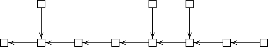


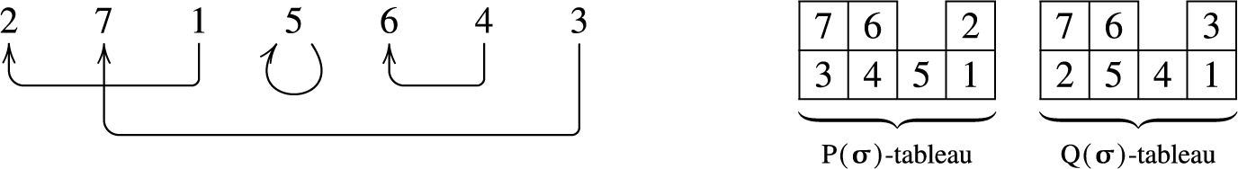


 Open access