


1 Introduction
In nearly all industrial applications and geophysical flows, turbulence is partly or completely wall bounded. In general, boundaries are not smooth but their surface is rather irregular and rough. Accordingly, such flows are extensively studied, although mainly under the approximation that the roughness is homogeneous (Jiménez Reference Jiménez2004). Homogeneously rough surfaces have a characteristic length scale  $k$ that is much smaller than the largest wall-normal length scale $\unicode[STIX]{x1D6FF}$. The effects of the roughness in these flows is believed to be confined to the immediate vicinity of the wall (i.e. the roughness sublayer), whereas in the outer, inertial layer, the flow only experiences the effective shear stress of the surface (Townsend’s outer layer similarity, Townsend Reference Townsend1976). As such, the focus of many studies is to find functional relationships between the parameters describing the roughness geometry and the skin friction coefficient $C_{f}$ (Flack & Schultz Reference Flack and Schultz2010). In practice, however, flows are bounded by rough boundaries that not only vary on the scale of $k$, but also on a much larger scale $s$, with $s=O(\unicode[STIX]{x1D6FF})$. Whereas these variations can occur either laterally (spanwise) or longitudinally (streamwise), we focus here only on the former. Such examples are found in shipping (i.e. the formation of stripes of bio-fouling on ship hulls (Schultz Reference Schultz2007)) and geophysical flows (e.g. the atmospheric flows over a spanwise-varying terrain (Ren & Wu Reference Ren and Wu2011)).
Hitherto, the research is focused on the effects of spanwise-varying rough surfaces on canonical systems of wall-bounded turbulence, i.e. pipe (Koeltzsch, Dinkelacker & Grundmann Reference Koeltzsch, Dinkelacker and Grundmann2002), boundary layer (Anderson et al. Reference Anderson, Barros, Christensen and Awasthi2015) and channel flow (Chung, Monty & Hutchins Reference Chung, Monty and Hutchins2018). The hallmark of flows over these surfaces is the presence of spanwise wall-normal secondary flows of size  $O(\unicode[STIX]{x1D6FF})$, with mean streamwise vorticity. Examples of studies where this has been observed are the works of Koeltzsch et al. (Reference Koeltzsch, Dinkelacker and Grundmann2002) on the effects of convergent and divergent grooves (reminiscent of shark skin) and the work by Wang & Cheng (Reference Wang and Cheng2006) on spanwise-varying riverbeds. We note that earlier research dates back to the works of Hinze (Reference Hinze1967, Reference Hinze1973) in the field of surface stress variations in duct flows.
Following up on the work of Koeltzsch et al. (Reference Koeltzsch, Dinkelacker and Grundmann2002), Nugroho, Hutchins & Monty (Reference Nugroho, Hutchins and Monty2013) set out to perform a parametric study of the converging–diverging riblet surface in a zero pressure gradient boundary layer (BL). They found a thickening of the BL height above the converging regions, and vice versa above the diverging regions. Furthermore, the energy spectra showed an increased energy content of the larger scales. Barros & Christensen (Reference Barros and Christensen2014) performed stereo particle image velocimetry (PIV) in the spanwise wall-normal plane for the flow over a turbine blade replica and found spanwise variations of the order of  $\unicode[STIX]{x1D6FF}$ in the mean velocity field. Within the same configuration, Mejia-Alvarez & Christensen (Reference Mejia-Alvarez and Christensen2013) identified regions of low momentum pathways (LMPs) and high momentum pathways (HMPs) in the instantaneous fields. Here, LMPs coincide with regions of enhanced turbulent kinetic energy (TKE) and Reynolds shear stress (RSS), and, rather remarkably, these regions do seem to occur at recessed roughness heights. Willingham et al. (Reference Willingham, Anderson, Christensen and Barros2014) found very similar behaviour of the secondary flows for a much more regular surface geometry. Vanderwel & Ganapathisubramani (Reference Vanderwel and Ganapathisubramani2015) found that only when $s/\unicode[STIX]{x1D6FF}\gtrapprox 0.5$ a secondary flow formation is observed. Here, $s$ is the spacing between streamwise aligned Lego® blocks. For $s/\unicode[STIX]{x1D6FF}\lessapprox 0.5$ the secondary flows are confined to the roughness sublayer. Interestingly, contrary to the findings of Mejia-Alvarez & Christensen (Reference Mejia-Alvarez and Christensen2013), they found LMPs on top of their elevated blocks, and HMPs in between the roughness strips. Yang & Anderson (Reference Yang and Anderson2017), however, found $s/H\gtrapprox 0.2$, with $H$ the channel half-height, as the threshold for heterogeneous behaviour of the streamwise aligned pyramid elements.
It is an open question as to why the varying experiments in the literature show conflicting orientations of the secondary flow. We note that there are some differences, namely that the experiments in the paper by Vanderwel & Ganapathisubramani (Reference Vanderwel and Ganapathisubramani2015) consist of small strips of elevated roughness, and wide regions of recessed roughness heights rather than alternating rough and smooth strips of equal width. One hypothesis concerns the location of the virtual origin of the rough part with respect to the smooth part. This could be either below (recessed) or above (protruding) the smooth surface, resulting in either an inflow (recessed) or an outflow (protruding) region above the roughness.
By carefully assessing the terms in the transport equation TKE, Anderson et al. (Reference Anderson, Barros, Christensen and Awasthi2015) found that spanwise variations of roughness lead to a local imbalance of production and dissipation of TKE, as already proposed by Hinze (Reference Hinze1967). Since the secondary flows are driven by a spatial gradient of the RSS, they find that the mean secondary flows are Prandtl’s secondary flow of the second kind (Bradshaw Reference Bradshaw1987). Medjnoun, Vanderwel & Ganapathisubramani (Reference Medjnoun, Vanderwel and Ganapathisubramani2018) observed a breakdown of outer layer similarity in the local profiles of the mean flow, turbulent intensity and the energy spectra, evidently induced by the presence of the secondary vortices. Finally, Chung et al. (Reference Chung, Monty and Hutchins2018) studied the influence of the spacing of idealized (i.e. no geometric induced disturbances to the flow) regions of low shear stress and high shear stress. They found that for  $s/\unicode[STIX]{x1D6FF}\lessapprox 0.39$ the notion of outer layer similarity is retained. Interestingly, for $s/\unicode[STIX]{x1D6FF}\gtrapprox 6.28$, they found a sign reversal of the isovels (stream velocity contour lines), with respect to the orientation of the secondary flows, that remain upwelling over low shear stress regions.
The aforementioned studies were all carried out in systems that lack two features which are intrinsic to many applications, namely the curvature in the streamwise direction (as in turbine blades), and the presence of strong secondary motions (as in the atmospheric boundary layer). Especially, the application for turbine blades is interesting, as also studied by Barros & Christensen (Reference Barros and Christensen2014). Here we come closer to this application by studying the turbulent flow over curved, rotating walls, present in the turbines.
1.1 Taylor–Couette flow
A canonical system in which these two properties can be observed simultaneously is the Taylor–Couette (TC) flow. TC flow is the flow between two coaxially, independently rotating cylinders. Its geometry is characterized by two dimensionless parameters; the radius ratio  $\unicode[STIX]{x1D702}=r_{i}/r_{o}$ and the aspect ratio $\unicode[STIX]{x1D6E4}=L/d$. Here, $r_{i}$ and $r_{o}$ are the inner cylinder radius and outer cylinder radius respectively, $L$ is the axial length of the inner cylinder and $d=r_{o}-r_{i}$ the gap between the two cylinders. Since TC is a closed system, one can directly relate global and local quantities through exact mathematical relations (Eckhardt, Grossmann & Lohse Reference Eckhardt, Grossmann and Lohse2007). The driving strength in TC flow is expressed in dimensionless form by the Taylor number
 $$\begin{eqnarray}Ta=\frac{1}{4}\unicode[STIX]{x1D70E}d^{2}\frac{(r_{i}+r_{o})^{2}(\unicode[STIX]{x1D714}_{i}-\unicode[STIX]{x1D714}_{o})^{2}}{\unicode[STIX]{x1D708}^{2}},\end{eqnarray}$$
 where  $\unicode[STIX]{x1D714}_{i}$ and $\unicode[STIX]{x1D714}_{o}$ are the inner and outer angular velocities of the cylinders, respectively, $\unicode[STIX]{x1D708}$ is the kinematic viscosity of the fluid and $\unicode[STIX]{x1D70E}=((1+\unicode[STIX]{x1D702})/(2\sqrt{\unicode[STIX]{x1D702}}))^{4}$ is the so-called geometric Prandtl number, in analogy to the Prandtl number in Rayleigh–Bénard convection (Eckhardt et al. Reference Eckhardt, Grossmann and Lohse2007). Alternatively, when the outer cylinder is at rest ( $\unicode[STIX]{x1D714}_{o}=0$), the driving strength can also be expressed with a Reynolds number based on the inner scales $Re_{i}=r_{i}\unicode[STIX]{x1D714}_{i}d/\unicode[STIX]{x1D708}$. This Reynolds number and $Ta~(\unicode[STIX]{x1D714}_{o}=0)$, are related by $Re_{i}=(8\unicode[STIX]{x1D702}^{2}/(1+\unicode[STIX]{x1D702})^{3})\sqrt{Ta}$. In TC flow, the angular velocity flux $J^{\unicode[STIX]{x1D714}}$ is radially conserved (Eckhardt et al. Reference Eckhardt, Grossmann and Lohse2007), where the effects of the top and bottom plates are assumed negligible. Here, $J^{\unicode[STIX]{x1D714}}=r^{3}(\langle u_{r}\unicode[STIX]{x1D714}\rangle _{A,t}-\unicode[STIX]{x1D708}(\unicode[STIX]{x2202}/\unicode[STIX]{x2202}r)\langle \unicode[STIX]{x1D714}\rangle _{A,t})$, where the brackets $\langle \cdot \rangle _{A,t}$ denote averaging over a cylindrical surface and time. The angular momentum flux for the case of laminar flow is $J_{lam}^{\unicode[STIX]{x1D714}}=2\unicode[STIX]{x1D708}r_{i}^{2}r_{o}^{2}(\unicode[STIX]{x1D714}_{i}-\unicode[STIX]{x1D714}_{o})/(r_{o}^{2}-r_{i}^{2})$. In this way, the response of the flow is quantified by the dimensionless Nusselt number ( $Nu_{\unicode[STIX]{x1D714}}$), which is also directly related to the torque ${\mathcal{T}}$ that is required to drive the cylinders at constant speed, i.e.
 $$\begin{eqnarray}Nu_{\unicode[STIX]{x1D714}}=\frac{J^{\unicode[STIX]{x1D714}}}{J_{lam}^{\unicode[STIX]{x1D714}}}=\frac{{\mathcal{T}}}{2\unicode[STIX]{x03C0}L\unicode[STIX]{x1D70C}J_{lam}^{\unicode[STIX]{x1D714}}}.\end{eqnarray}$$
 Here,  $\unicode[STIX]{x1D70C}$ is the density of the working fluid. Alternatively, the torque of the system can be non-dimensionalized to form the friction coefficient $C_{f}={\mathcal{T}}/(\unicode[STIX]{x1D70C}L\unicode[STIX]{x1D708}^{2}Re_{i}^{2})$, which is directly related to the Nusselt number,
 $$\begin{eqnarray}Nu_{\unicode[STIX]{x1D714}}=C_{f}\unicode[STIX]{x1D714}_{i}(r_{o}-r_{i})^{2}(r_{o}^{2}-r_{i}^{2})/(4\unicode[STIX]{x03C0}\unicode[STIX]{x1D708}r_{o}^{2}).\end{eqnarray}$$
 The inner friction velocity  $u_{\unicode[STIX]{x1D70F},i}$ is also related to the torque by $u_{\unicode[STIX]{x1D70F},i}=\sqrt{{\mathcal{T}}/(2\unicode[STIX]{x03C0}r_{i}^{2}\unicode[STIX]{x1D70C}L)}$, which is used to scale quantities in the inner layer, indicated with the superscript ‘ $+$’. The friction angular velocity $\unicode[STIX]{x1D714}_{\unicode[STIX]{x1D70F}}$ equals $u_{\unicode[STIX]{x1D70F}}/r$. Lastly, a frictional Reynolds number based on the inner scales can be defined as $Re_{\unicode[STIX]{x1D70F}}=u_{\unicode[STIX]{x1D70F},i}d/(2\unicode[STIX]{x1D708})$.
Secondary flows are featured in TC flow, in the form of large-scale vortices with a mean streamwise vorticity component, the so-called turbulent Taylor vortices (TTVs). These structures are reminiscent of laminar Taylor vortices, which transition through a series of instabilities into turbulence once the flow becomes unstable (Taylor Reference Taylor1923). As noted by Chouippe et al. (Reference Chouippe, Climent, Legendre and Gabillet2014), the axial wavelength  $\unicode[STIX]{x1D706}/d$ of the TTVs, i.e. the distance between two rolls, is primarily a function of $\unicode[STIX]{x1D702}$ and $Re$. When $Re$ is large enough ( $O(10^{6})$), the rolls are observed to persist in the system (Huisman et al. Reference Huisman, van der Veen, Sun and Lohse2014). Here, multiple states for $\unicode[STIX]{x1D702}=0.716$ can be observed in a certain regime of counter-rotating cylinders, namely $a\in [0.17,0.51]$, where $a=-\unicode[STIX]{x1D714}_{o}/\unicode[STIX]{x1D714}_{i}$ is their rotation ratio. These multiple states are characterized by a change in the number of rolls present in the system and, as a consequence, in their averaged axial wavelength ( $\unicode[STIX]{x1D706}/d=1.46$ or $\unicode[STIX]{x1D706}/d=1.96$). These states, with the transition between them being strongly hysteretic, even at $Re=O(10^{6})$ (Huisman et al. Reference Huisman, van der Veen, Sun and Lohse2014; van der Veen et al. Reference van der Veen, Huisman, Dung, Tang, Sun and Lohse2016; Gul, Elsinga & Westerweel Reference Gul, Elsinga and Westerweel2017), result in different torques for the same rotation rates, which reflects the importance of the large-scale structures (TTV) in transporting angular momentum. At pure inner cylinder rotation however ( $a=0$), no multiple states are found and the rolls are observed to be less coherent and stable. Finally, we note that the effect of the curvature of the cylinders is quantified by the radius ratio $\unicode[STIX]{x1D702}$, and it has a tremendous impact on the flow organization, as was reported by Ostilla-Mónico et al. (Reference Ostilla-Mónico, Huisman, Jannink, Van Gils, Verzicco, Grossmann, Sun and Lohse2014a,Reference Ostilla-Mónico, van der Poel, Verzicco, Grossmann and Lohseb). For a detailed review on turbulent Taylor–Couette flow we refer the reader to the review of Grossmann, Lohse & Sun (Reference Grossmann, Lohse and Sun2016).
Roughness in a TC geometry has been studied in various ways: Cadot et al. (Reference Cadot, Couder, Daerr, Douady and Tsinober1997) and van den Berg et al. (Reference van den Berg, Doering, Lohse and Lathrop2003) used obstacle roughness, in the form of axial riblets, to study the scaling of the angular momentum transport with the driving strength. Zhu et al. (Reference Zhu, Ostilla-Mónico, Verzicco and Lohse2016) investigated the influence of grooves for large  $Ta~(O(10^{10}))$, and found that at the tips of the grooves, plumes are preferentially ejected. In a more recent work, Zhu et al. (Reference Zhu, Verschoof, Bakhuis, Huisman, Verzicco, Sun and Lohse2018) found that, by using a similar configuration of rough walls as in van den Berg et al. (Reference van den Berg, Doering, Lohse and Lathrop2003), the scaling $Nu_{\unicode[STIX]{x1D714}}\propto Ta^{1/2}$, where the logarithmic corrections of the ultimate regime vanish for asymptotically high Reynolds numbers, is obtained. This regime is referred to as the asymptotic ultimate regime (Grossmann et al. Reference Grossmann, Lohse and Sun2016; Zhu et al. Reference Zhu, Verschoof, Bakhuis, Huisman, Verzicco, Sun and Lohse2018). They attribute this to a dominance of the pressure drag over the viscous drag on the cylinders. Very recently, Berghout et al. (Reference Berghout, Zhu, Chung, Verzicco, Stevens and Lohse2019) studied the influence of sandgrain roughness in TC flow, and found similarity of the roughness function with the same type of roughness in pipe flow (Nikuradse Reference Nikuradse1933). None of the TC papers described above reported an influence of the roughness variations in the axial direction, i.e. the spanwise direction.
In this paper we will fill this gap and study the effects of spanwise-varying roughness in highly turbulent TC flow with  $Ta$ up to $O(10^{12})$, for the case of pure inner cylinder rotation $a=0$, where secondary flows are present in the form of TTVs. In particular, we focus on the effect of spanwise-varying roughness on the TTVs and, thus, on the global and local response of the flow. We introduce the roughness through a series of stripes which extend along the entire circumference of the inner cylinder (IC). This gives rise to a spanwise (axial) arrangement of roughness which we characterize with the widths of the roughness stripe. We conduct both experiments and direct numerical simulations (DNS) for various dimensionless stripe widths $\tilde{s}=s/d$, i.e. the width of the roughness stripe normalized with the gap width. For practical reasons, the roughness area is slightly larger than the smooth area, with a rough area coverage of 56 %.
The structure of the paper is as follows. In § 2, we introduce the experimental and numerical methods. In § 3.1 we show the local response of the flow due to the varying roughness arrangement. In § 3.2, we study its effect on the global quantities. In § 3.3, we link the global and local observations and explain the physical mechanism between the interaction of the rolls and the roughness. We finalize the paper in § 4 with some conclusions and an outlook to future work.
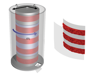
(a) Schematic of the Twente Turbulent Taylor–Couette facility showing the sandpaper roughness on the inner cylinder in red. PIV measurements in the  $r{-}\unicode[STIX]{x1D703}$ plane become possible thanks to illumination from the side with a high-power pulsed laser, creating a horizontal sheet. The sheet is imaged through a window and a mirror in the bottom of the set-up. Using laser Doppler anemometry, the streamwise velocity is measured along the spanwise direction. The torque is measured in the middle section of the IC (highlighted in blue), which has a length of $L_{mid}=536~\text{mm}$ (van Gils et al. Reference van Gils, Huisman, Grossmann, Sun and Lohse2012). (b) Numerical domain for the case of $\tilde{s}\equiv s/d=0.47$. The sandpaper roughness is taken from a confocal scan of the material used in the experiment, see figure 2.

2 Methods
2.1 Numerical methods
The radius ratio  $\unicode[STIX]{x1D702}=0.714$, the same as in the experiments. The streamwise and spanwise lengths of the computational domain are set to match the minimum computational domain size as studied in Ostilla-Mónico et al. (Reference Ostilla-Mónico, van der Poel, Verzicco, Grossmann and Lohse2014c). As such, we simulate aspect ratios of $2.0\leqslant \unicode[STIX]{x1D6E4}\leqslant 3.32$ with periodic boundary conditions in the axial direction. The mean roughness height $\langle h_{r}\rangle /d=0.02$ is small, so that the effective radius ratio is only slightly affected. We scale the roughness stripe such that the maximum roughness height, and thus the maximum blockage ratio, was $\max (h_{r})=0.1d$. Depending on $\tilde{s}$, we cut out a portion of roughness from the scanned surface. The roughness was then mirrored and concatenated to obtain a streamwise homogeneous spanwise periodic stripe.
The sandpaper roughness was implemented in the code by an immersed boundary method (IBM) (Fadlun et al. Reference Fadlun, Verzicco, Orlandi and Mohd-Yusof2000). In the IBM, the boundary conditions were enforced by adding a body force  $\boldsymbol{f}$ to the Navier–Stokes equations. A regular, non-body fitting, mesh can thus be used, even though the rough boundary has a very complex geometry. We perform interpolation in the spatial direction preferential to the normal surface vector to transfer the boundary conditions to the momentum equations. The IBM has been validated previously (Fadlun et al. Reference Fadlun, Verzicco, Orlandi and Mohd-Yusof2000; Iaccarino & Verzicco Reference Iaccarino and Verzicco2003; Stringano, Pascazio & Verzicco Reference Stringano, Pascazio and Verzicco2006; Zhu et al. Reference Zhu, Ostilla-Mónico, Verzicco and Lohse2016). A moving average over $10\times 10$ points is employed to smooth the scan from measurement noise. Finally, we set the resolution based on the demands ( $\unicode[STIX]{x0394}z^{+},r_{i}^{+}\unicode[STIX]{x0394}\unicode[STIX]{x1D703}<3$), which is small enough to recover the smallest geometrical features of the surface.
2.2 Experimental apparatus with spanwise roughness
The experiments have been performed in the Twente Turbulent Taylor–Couette ( $\text{T}^{3}\text{C}$) facility as shown in figure 1(a) (details of the experimental facility can be found in van Gils et al. (Reference van Gils, Bruggert, Lathrop, Sun and Lohse2011)). The inner cylinder has a radius $r_{i}=200~\text{mm}$ and the outer cylinder has a radius $r_{o}=279.4~\text{mm}$, such that the gap size is $d=r_{o}-r_{i}=79.4~\text{mm}$, and the radius ratio $\unicode[STIX]{x1D702}=r_{i}/r_{o}=0.716$. To minimize the effects of the endplate on the torque signal, the inner cylinder is partitioned into three sections and the torque is only measured at the middle section ( $L_{mid}=536~\text{mm}$), shown as the highlighted section in figure 1a). The combined length of the cylinders is $L=927~\text{mm}$, which leads to an aspect ratio $\unicode[STIX]{x1D6E4}=L/d=11.7$. The outer cylinder (OC), is made of transparent acrylic which allows for optical access to the flow. The working fluid is demineralised water. We apply spanwise-varying roughness to the inner cylinder, which leads to patterns of homogeneously rough and hydrodynamically smooth bands in the spanwise direction (see figure 1a). The rough stripes are made of P36 ceramic industrial grade sandpaper and are fixed to the IC using double-sided adhesive tape ( ${\approx}1~\text{mm}$). In figure 2, we show the height scan of a roughness element using confocal microscopy. The scan revealed that the height ( $h_{r}$) of the roughness is mostly within $\pm 2\unicode[STIX]{x1D70E}(h_{r})$ of the mean, giving a characteristic length scale $k\equiv 4\unicode[STIX]{x1D70E}(h_{r})=695~\unicode[STIX]{x03BC}\text{m}$ (see figure 2b). More statistics of the roughness are shown in table 1. We fix the surface coverage of the roughness at $56\,\%$ such that $0.56A_{i}$ of the cylinder is rough, where $A_{i}=2\unicode[STIX]{x03C0}r_{i}L$ is the area of the entire IC. The middle section of the inner cylinder has a constant coverage of 56 %.
(a) Height scan captured using confocal microscopy of a patch of sandpaper of size  $20~\text{mm}\times 20~\text{mm}$ with a resolution of $2.5~\unicode[STIX]{x03BC}\text{m}$. The typical size of the grains is given by $k\equiv 4\unicode[STIX]{x1D70E}(h_{r})=695~\unicode[STIX]{x03BC}\text{m}$ where $h_{r}$ is the height and $\unicode[STIX]{x1D70E}$ the standard deviation. The normalized typical grain size is then $k/d\approx 0.01$. (b) Probability density function (PDF) of the measured height of the roughness stripe, with subtracted mean $h_{r}^{\prime }=h_{r}-\langle h_{r}\rangle$.

Various statistics of the roughness  $h_{r}^{\prime }=h_{r}-\langle h_{r}\rangle$ based on the data obtained from confocal microscopy, see also figure 2. $\langle h_{r}\rangle$ is the distance with respect to the smooth cylinder surface. These values represent the actual roughness used in experiments; in DNS a scaled version of these values are used.

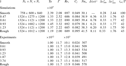
List of parameters involved in both the simulations and the experiments.  $\tilde{s}=s/d$ is the normalized roughness width with smooth and rough indicating the fully smooth and fully rough cases respectively (i.e. 0 % or 100 % coverage of sandpaper roughness). $N_{\unicode[STIX]{x1D703}}\times N_{z}\times N_{r}$ is the numerical resolution in the streamwise, spanwise and radial directions, respectively. $\unicode[STIX]{x1D6E4}=L/d$ is the aspect ratio and $L_{\unicode[STIX]{x1D703}}=r_{i}\frac{1}{3}\unicode[STIX]{x03C0}$ is the constant streamwise length of the domain. $\unicode[STIX]{x1D6E5}(\unicode[STIX]{x1D714})^{+}$ is the downward shift of the angular velocity profile $\unicode[STIX]{x1D714}^{+}$. $\unicode[STIX]{x0394}r_{min}^{+}$ is the minimum spacing in the wall-normal direction at the location of the maximum roughness height. $\unicode[STIX]{x0394}r_{max}^{+}$ is the maximum spacing in the wall-normal direction. $r_{i}^{+}\unicode[STIX]{x0394}\unicode[STIX]{x1D703}=\unicode[STIX]{x0394}z^{+}\approx 2.7$ ( $r_{o}^{+}\unicode[STIX]{x0394}\unicode[STIX]{x1D703}\approx 3.8$) is the grid spacing in the streamwise and spanwise directions. In the DNS, the roughness height $k^{+}=4\unicode[STIX]{x1D70E}(h_{r})^{+}=130\pm 1$ for all rough cases. $t_{av}/T$ is the averaging time needed to collect statistics, normalized with the bulk flow time scale $T=d/(r_{i}(\unicode[STIX]{x1D714}_{i}-\unicode[STIX]{x1D714}_{o}))$. All experimental $Nu_{\unicode[STIX]{x1D714}}$ are based on global torque measurements.
2.2.1 Global measurements: torque
We measured the torque  ${\mathcal{T}}$ needed to drive the inner cylinder at constant angular velocity (the outer cylinder is kept at rest). For this we used a hollow flange reaction torque transducer connecting the drive shaft and the inner cylinder, sampled at 100 Hz. We continuously measured the torque while quasi-statically ramping the frequency of the inner cylinder, $f_{i}$, from 5 to 18 Hz, with increments of $0.002~\text{Hz}~\text{s}^{-1}$. This corresponds to $Ta$ between $4\times 10^{11}$ and $Ta\approx 6\times 10^{12}$. The system is temperature controlled such that all the experiments were performed at $21\pm 1~^{\circ }\text{C}$ and all fluid flow properties are calculated at their actual temperature. Table 2 shows additional experimental parameters.
2.2.2 Local measurements: LDA and PIV
We performed a spanwise scan of the streamwise velocity with laser Doppler anemometry (LDA). The scan was performed at the middle of the gap,  $\tilde{r}=(r-r_{i})/d=0.5$, at a fixed $Ta=9.5\times 10^{11}$. Due to the axial symmetry, we scan the flow from mid-height to the bottom of the system. The flow was seeded using $5~\unicode[STIX]{x03BC}\text{m}$-diameter polyamide particles with a density of $1030~\text{kg}~\text{m}^{-3}$ that act as passive tracers (van Gils et al. Reference van Gils, Huisman, Grossmann, Sun and Lohse2012). The laser beams went through the outer cylinder and were focused in the middle of the gap. We corrected for curvature effects (and refractive index effects) by numerically ray tracing the LDA beams, as was shown in Huisman, van Gils & Sun (Reference Huisman, van Gils and Sun2012). The spanwise extent of the LDA scans was $0\leqslant z/L\leqslant 0.5$. Particle image velocimetry measurements were performed at $Ta=9.5\times 10^{11}$ (same as LDA) in the radial–azimuthal plane. The scan was performed for various heights and for all $\tilde{s}$. For the PIV measurements the flow was seeded with different particles that act as passive tracers, namely, fluorescent polymer particles (Dantec FPP-RhB-10) with diameters of $1{-}20~\unicode[STIX]{x03BC}\text{m}$ with a seeding density of ${\approx}0.01~\text{particles}~\text{pixel}^{-1}$. These particles have an emission peak with a wavelength of ${\approx}565~\text{nm}$. We illuminated the particles with a Quantel Evergreen 145 532 nm, double pulsed laser. A cylindrical lens was used to create a light sheet of ${\approx}1~\text{mm}$ thickness. The height of the laser sheet is altered using a custom traverse system. The images were captured with an Imager SCMOS ( $2560\times 2160$ pixel) 16 bit camera with a Carl Zeiss 2.0/100 lens through a window in the bottom plate of the set-up and a mirror. The camera was operated in double frame mode with a frame rate $f=15~\text{Hz}$ which was much smaller than the inverse interframe time $1/\unicode[STIX]{x0394}t$, i.e. $\unicode[STIX]{x0394}t\ll 1/f$. In order to enhance the particle contrast in the images, we added an Edmund High-Performance Longpass 550 nm filter to the camera lens. For every $\tilde{s}$, the spanwise extent of the experiments was different. This is done because – as will be shown later – the aspect ratios of the rolls change depending on $\tilde{s}$. For the smallest $\tilde{s}=0.63$ however, the spanwise resolution was $\unicode[STIX]{x1D6FF}z/L\approx 0.011$ while for the largest value $\tilde{s}=3.74$, $\unicode[STIX]{x1D6FF}z/L\approx 0.022$. Since we scan in the spanwise direction, the focus of the camera was changed accordingly. For each height, 1000 image pairs were recorded. The fields were resolved with a commercial PIV software (Davis 8.0) based on a multi-step method. The initial interrogation window size was set to $64\times 64~\text{pixels}$ and it decreased to $32\times 32$ pixels for the last iteration, for increased accuracy. The fields are calculated in Cartesian coordinates, which we transformed to polar coordinates. The final result were the fields in the form $\boldsymbol{u}=u_{r}(r,\unicode[STIX]{x1D703},t)\hat{e_{r}}+u_{\unicode[STIX]{x1D703}}(r,\unicode[STIX]{x1D703},t)\hat{e_{\unicode[STIX]{x1D703}}}$, where $u_{r}$ and $u_{\unicode[STIX]{x1D703}}$ are the radial and streamwise velocity components which depend on the radius $r$, the azimuthal (streamwise) direction $\unicode[STIX]{x1D703}$ and time $t$. For an example of a typical azimuthal velocity field obtained from the experiments, see figure 3.
Time average of the azimuthal velocity  $\langle u_{\unicode[STIX]{x1D703}}\rangle _{t}$ obtained from PIV measurements for the case of $s/d=1.23$ and $\tilde{z}=0.48$. The resolution of the image field at this height is $9~\text{cm}/2560~\text{px}\approx 35~\unicode[STIX]{x03BC}\text{m}~\text{px}^{-1}$. The colour bar and the length of the vectors depict the value of the azimuthal velocity normalized with the inner velocity $u_{i}=r_{i}\unicode[STIX]{x1D714}_{i}$. For clarity, the vector field is sub-sampled approximately $10\times$. The data that lie within $0.02d$ of both the inner and the outer cylinders are omitted as not enough resolution is available to measure the structure of the boundary layers. The black solid lines represent the inner and outer cylinders, respectively.

Snapshot of the instantaneous angular velocity with the mean angular velocity subtracted, for  $Ta\approx O(10^{9})$. We observe the formation of plumes from the roughness elements whereas very few plumes are formed above the smooth patches.

3 Results
3.1 Response of the turbulent Taylor vortices
3.1.1 Laser Doppler anemometry
(a) Normalized standard deviation of the streamwise velocity  $\unicode[STIX]{x1D70E}(u_{\unicode[STIX]{x1D703}})/u_{i}$ at mid-gap, as a function of $\tilde{z}=z/d$ for various $\tilde{s}$. Experimental data are captured using LDA while $Ta$ is fixed at $1\times 10^{12}$. For DNS, $Ta$ is set to $O(10^{9})$ for all cases. The enforced roughness pattern is indicated in a red vertical line and a light blue shade. The signature of the roughness pattern is clearly visible in the bulk flow, both for the numerical simulations (orange) as for the experiments (blue). For $\tilde{s}=0.61$, the roughness pattern does not leave a distinct imprint of its topology in the mid-gap flow statistics. Fully smooth and fully rough reference cases from experiments are shown as dotted lines. (b) Local friction factor $c_{f}(\tilde{z})$ versus the axial height $\tilde{z}=z/d$ for $Ta=O(10^{9})$, based on DNS data. The black lines show $c_{f}(\tilde{z})$ at the IC and the green lines show $c_{f}(\tilde{z})$ at the OC. $c_{f,r}$ above the rough patches was calculated by subtracting the smooth average of $c_{f,s}$ from $C_{f}=\langle c_{f}(\tilde{z})\rangle _{L}$ of the entire IC. Hatched regions indicate spanwise translated copies of the same data (including averages) – possible due to the periodic boundary condition in the axial direction – to allow for straightforward comparison. Imprints of the large secondary flows on the friction at the cylinder walls is observed, where impacting region experience a higher shear stress.

In order to get a first insight into the effect of the roughness on the flow, we performed spanwise scans of the streamwise flow velocity at mid-gap using LDA. Subsequently, we calculated the standard deviation of the streamwise velocity. The experiments will be compared with the simulations. Figure 4 shows an example of the snapshot of the instantaneous angular velocity from the simulations. In figure 5(a), we show the standard deviation of the streamwise velocity  $\unicode[STIX]{x1D70E}(u_{\unicode[STIX]{x1D703}})$ normalized by the inner cylinder velocity $u_{i}$, as a function of the height, for various $\tilde{s}$. Here, the spanwise coordinate is normalized using the cylinder gap width $d$ such that $\tilde{z}=z/d$. In the top row, we compare the results from direct numerical simulations and experiments. Since we employ different boundary conditions in the spanwise direction in DNS (periodic) and experiments (stationary solid plates), the comparison will be most reliable at mid-height, where end effects are negligible. Therefore, we overlay the results from DNS (orange lines) over the results from experiments (blue lines) at matching locations with respect to the roughness stripes, at $\tilde{z}\in (1,6)$. In the bottom row we only assess the results from DNS and consequently plot $\tilde{z}\in (0,\unicode[STIX]{x1D6E4})$.
Figure 5(a) reveals that, for the case of the largest stripe width ( $\tilde{s}=3.74$), the smooth section has, on average, a value of $\unicode[STIX]{x1D70E}(u_{\unicode[STIX]{x1D703}})/u_{i}\approx 0.03$, slightly larger than we found for the fully smooth case (shown with the dotted light blue lines). Above the rough stripe, towards the centre of the set-up (i.e. for large $\tilde{z}$), $\unicode[STIX]{x1D70E}(u_{\unicode[STIX]{x1D703}})$ gradually increases to a value of approximately $\unicode[STIX]{x1D70E}(u_{\unicode[STIX]{x1D703}})/u_{i}\approx 0.04$. A similar, but not so clear trend can be seen at the lower roughness section ( $\tilde{z}\approx 0.93$) of this case. However, this might be influenced by the lower bottom plate of the system.
When looking at the  $\tilde{s}=1.87$ case, we see very similar, however more pronounced, dynamics. Streamwise velocity fluctuations are promoted in regions where the roughness is present, as suggested by the appearance of local peaks centred at the position of the rough stripes. This effect is further seen for the cases $\tilde{s}=1.23$ and $\tilde{s}=0.93$, where we observe similar profiles. At their smooth areas however, we also observe enhanced velocity fluctuations, albeit less pronounced than the locations above the rough patches. This effect is not seen for $\tilde{s}>1.27$. For the final case with $\tilde{s}=0.61$ these trends seems to fade away and we see that $\unicode[STIX]{x1D70E}(u_{\unicode[STIX]{x1D703}})$ becomes more spanwise independent, i.e. the peaks are less pronounced, and do not seem to follow the topology of the roughness stripes.
The results of the DNS, presented together with the experiments in figure 5(a) exhibit very similar behaviour. When normalized with  $u_{i}$, we find that the standard deviation of the streamwise velocity shows similar values as in the experiments. This is intriguing since the $k/d$ values in the simulations are almost one order of magnitude larger than in the experiments. Above the rough stripes, we find enhanced $\unicode[STIX]{x1D70E}(u_{\unicode[STIX]{x1D703}})/u_{i}$, whereas over smooth stripes we find diminished $\unicode[STIX]{x1D70E}(u_{\unicode[STIX]{x1D703}})/u_{i}$. For $\tilde{s}=0.61$ however, the trends are somewhat different. There, we find enhanced $\unicode[STIX]{x1D70E}(u_{\unicode[STIX]{x1D703}})/u_{i}$ above the smooth region in the DNS, which is explained by the recombination of plume ejection regions, forming one larger TTV above the smooth regions, see figure 7.
The findings presented in figure 5(a) show that the presence of the roughness affects the relative turbulence statistics in the bulk of the flow, far away from the roughness sublayer region (in contrast to homogeneous roughness in TC flow (Berghout et al. Reference Berghout, Zhu, Chung, Verzicco, Stevens and Lohse2019)), reminiscent to what is found in studies of pipe and channel flows (Koeltzsch et al. Reference Koeltzsch, Dinkelacker and Grundmann2002; Chung et al. Reference Chung, Monty and Hutchins2018).
Figure 5(b) shows the spanwise variations of the friction factor  $c_{f}(\tilde{z})$ (see § 1) on both the inner cylinder and the outer cylinder. The solid and dashed black lines represent $c_{f}(\tilde{z})$ measured on the inner cylinder, and the solid (green) lines represent $c_{f}(\tilde{z})$ on the outer cylinder. We average both in time and in the streamwise direction. Significant variations in $c_{f}(\tilde{z})$ are observed which are linked to the orientation of the TTV. For impacting regions, i.e. plumes impacting on the inner cylinder boundary layer, the wall shear stress in the streamwise direction is enhanced. When plumes are ejected from the inner cylinder boundary layer, also known as the ejecting regions, the shear stress is reduced. This, once more, illustrates the relative strength of the secondary flow (TTV) and the mean flow. For $\tilde{s}=0.93$, the variations of the friction factor on the outer cylinder are even more pronounced, thus indicating that the strengths of the TTV are enhanced with enforcing the spanwise variations in the roughness. For $\tilde{s}=0.47$, the variations are not visible and the TTVs are severely weakened, but still present, see figure 7.
3.1.2 Particle imaging velocimetry and direct numerical simulations
Temporal and streamwise average of the radial velocity  $u_{r}$, normalized with the inner cylinder streamwise velocity $u_{i}$, obtained from experiments at $Ta=1\times 10^{12}$ using PIV for varying roughness stripe sizes $\tilde{s}$. A positive value of $u_{r}$ denotes outflow, while a negative value denotes inflow, with respect to the inner cylinder. It can be seen that the rolls are pinned by the roughness and their wavelength changes with $\tilde{s}$. The red and grey areas at the left side of each plot indicate the positions of the rough and smooth areas, respectively. Note that the typical grain size is $k/d\approx 0.01$. The grey shaded areas in the gap represent unexplored heights.

Deviation of the temporal and streamwise averaged angular velocity  $\langle \unicode[STIX]{x1D714}\rangle _{t,\unicode[STIX]{x1D703}}$ with respect to the temporal, streamwise and spanwise averaged angular velocity $\langle \unicode[STIX]{x1D714}\rangle _{t,\unicode[STIX]{x1D703},z}$ obtained from DNS at $Ta\approx O(10^{9})$ (top), and experiments at $Ta=1\times 10^{12}$ (bottom), for various $\tilde{s}$ explored. For experiments, $\tilde{r}$ spans $[0.05,0.95]$. All fields are normalized with the angular velocity of the inner cylinder $\unicode[STIX]{x1D714}_{i}=u_{i}/r_{i}$. Positive values represent velocities that are closer to the IC velocity. The leftmost panel corresponds to the case of no roughness (smooth) while the rightmost panel is the case where the entire IC is uniformly rough. For better comparison, overlapping $\tilde{s}$ cases for DNS and experiments are aligned vertically. Missing cases are not feasible in experiments or DNS. Hatched regions in the DNS figures indicate spanwise translated copies of the same data – possible due to the periodic boundary condition in the spanwise direction – to allow for straightforward comparison. The grey shaded areas in the gap represent unexplored heights. Ejecting regions can be seen in spanwise locations where the roughness is present. Notice the similarity of the flow structures between DNS and experiments.

(a) Compensated global Nusselt number  $Nu_{\unicode[STIX]{x1D714}}Ta^{-0.45}$ as a function of $Ta$ for varying $\tilde{s}$, based on torque measurements. The shaded area indicates the error based on the standard deviation from repeated measurements, which can be seen to decrease with increasing driving strength. (b) Compensated global Nusselt number $Nu_{\unicode[STIX]{x1D714}}Ta^{-0.45}$ as a function of $\tilde{s}$ for three selected $Ta$, again calculated from torque measurements. Here, an optimum value in the transport of angular momentum is observed close to $\tilde{s}\approx 1$. We note that the optimum could in principle be located anywhere in the range $0.61<\tilde{s}<1.23$. More experiments in this domain are needed to pinpoint the location of the maximum. The inset in (b) shows the results obtained with the DNS ( $Ta\approx 10^{9}$), where the maximum can be observed at a slightly lower $\tilde{s}$, namely $\tilde{s}\approx 0.6$. (c) The strength of the rolls, quantified as the normalized root mean square of the radial velocity $\tilde{u} _{r}^{\prime }$ as a function of $\tilde{s}$, for both, DNS and experiments. Solid and dashed lines show fully smooth and rough cases respectively. The inset shows the wavelength of the TTV as a function of $\tilde{s}$. (d) Global friction coefficient $C_{f}$ as a function of the driving strength, expressed with the Reynolds number $Re_{i}$, for various $\tilde{s}$, based on the torque data. The order of the curves is identical to figure 6(a). For fully smooth and fully rough, the best fits of the Prandtl friction law are shown.

To gain more insight into how the roughness alters the flow, we set out to measure the velocity field in the meridional plane using PIV at multiple heights. For the cases that required the highest axial resolution ( $\tilde{s}=0.61$ and $\tilde{s}=0.93$) of the PIV measurements we employed $\unicode[STIX]{x1D6FF}_{z}/d\approx 0.13$, where $\unicode[STIX]{x1D6FF}_{z}$ is the spacing of laser sheets in $z$, so that every TTV roll pair was at least sampled $7$ times. This is enough to resolve the wavelength of the structure. For all other $\tilde{s}$, the sample resolution is higher than 7 times per wavelength. In figure 6, we show the temporal and streamwise averaged radial velocity component $u_{r}$, normalized with $u_{i}$, in the spanwise–wall-normal plane ( $\tilde{z}-\tilde{r}$), where the radial coordinate is normalized such that $\tilde{r}=(r-r_{i})/d$. Figure 6 shows that for the case of $\tilde{s}=3.74$, a very large structure can be seen, which consists of a large outflow region (positive $u_{r}$) around $\tilde{z}=5.84$, while a large inflow region (negative $u_{r}$) is detected around $\tilde{z}=2.10$. The situation is more pronounced for the cases of $\tilde{s}=1.87$, $\tilde{s}=1.23$ and $\tilde{s}=0.93$, where a clear roll-like structure (i.e. the TTV) can be observed. Note that the radial component in the flow changes sign along the spanwise direction as it should in the presence of a TTV. What is rather remarkable is that the wavelength of the rolls $\unicode[STIX]{x1D706}$ changes for different values of $\tilde{s}$. For the large structure at $\tilde{s}=3.74$, the normalized wavelength is $\tilde{\unicode[STIX]{x1D706}}=\unicode[STIX]{x1D706}/d\approx 4.01$. As $\tilde{s}$ decreases to $\tilde{s}=1.87$, $\tilde{\unicode[STIX]{x1D706}}\approx 1.49$. At $\tilde{s}=1.23$, the wavelength decreases to a value of $\tilde{\unicode[STIX]{x1D706}}\approx 1.42$. At $\tilde{s}=0.93$, $\tilde{\unicode[STIX]{x1D706}}\approx 0.94$, and finally for the smallest value of $\tilde{s}=0.61$, the wavelength increases slightly to $\tilde{\unicode[STIX]{x1D706}}=1.09$. We remind the reader of the work of Huisman et al. (Reference Huisman, van der Veen, Sun and Lohse2014), who revealed that for counter-rotation ( $-\unicode[STIX]{x1D714}_{o}/\unicode[STIX]{x1D714}_{i}\approx 0.4$), the average wavelength of the rolls could be either $\tilde{\unicode[STIX]{x1D706}}=1.46$ or $\tilde{\unicode[STIX]{x1D706}}=1.96$ depending on the state attained by the system. The current work shows that, by an appropriate choice of $\tilde{s}$, the wavelength of the rolls can firstly, abandon its natural state, and secondly, it can be tuned within the range $\tilde{\unicode[STIX]{x1D706}}\in [0.94,4.01]$. The wavelengths described above were calculated by measuring the locations of two consecutive maxima and minima of $\langle u_{r}\rangle _{t,\unicode[STIX]{x1D703},r_{bulk}}$ along $z$ which are closest to mid-height. Here, the symbol $\langle \cdot \rangle _{t,\unicode[STIX]{x1D703},r_{bulk}}$ denotes average over time, the streamwise direction and the bulk region, i.e. $(r_{bulk}-r_{i})/d\in [0.3,0.7]$.
In addition, we observe that outflow regions (flow away from the IC) are created in spanwise regions where the roughness is located; and conversely, inflow regions (flow towards the IC) are created in the smooth areas. Note that this orientation of the secondary flows is opposite to what is found in other canonical systems (e.g. pipe flow and channel flow (Willingham et al. Reference Willingham, Anderson, Christensen and Barros2014; Yang & Anderson Reference Yang and Anderson2017; Chung et al. Reference Chung, Monty and Hutchins2018)), where one finds inflow regions above the rough stripes and outflow regions above the smooth stripes. Consistent with findings in boundary layers however, is the correlation between low momentum pathways and outflow regions (Vanderwel & Ganapathisubramani Reference Vanderwel and Ganapathisubramani2015). Indeed we find that LMPs – with respect to the IC and located on top of the roughness – are associated with outflow regions, similar to Vanderwel & Ganapathisubramani (Reference Vanderwel and Ganapathisubramani2015) although their Lego® roughness strips are much thinner and protrudes farther into the flow.
Another interesting observation is that, since the driving is now from the BL rather than the bulk, the strength of the rolls changes depending on the value of  $\tilde{s}$, as evidenced by the magnitude of $|u_{r}|$. In order to explore this feature in more detail, we quantify the strength of the rolls by $\tilde{u_{r}}^{\prime }\equiv \sqrt{\langle (u_{r}/u_{i})^{2}\rangle _{t,\unicode[STIX]{x1D703},r_{bulk},z_{\unicode[STIX]{x1D706}}}}$ as a function of $\tilde{s}$. Here, the symbol $\langle \cdot \rangle _{t,\unicode[STIX]{x1D703},r_{bulk},z_{\unicode[STIX]{x1D706}}}$ denotes an average over time, the streamwise direction, the bulk region and the spanwise region that defines the wavelength of a single roll $z_{\unicode[STIX]{x1D706}}$. In figure 8(c), we show $\tilde{u_{r}}^{\prime }$ as a function of $\tilde{s}$, where we observe that the strength of the rolls increases with decreasing $\tilde{s}$ for $\tilde{s}\in [0.93,3.74]$. However at $\tilde{s}=0.61$ the trend is broken, and we observe that $\tilde{u_{r}}^{\prime }$ decreases with respect to the case of $\tilde{s}=0.93$.
In order to obtain more insight into the mechanism(s) that lead to the variation of  $\tilde{\unicode[STIX]{x1D706}}$ with $\tilde{s}$, we turn to DNS, albeit at a much lower $Ta~({\approx}1.0\times 10^{9})$, and much higher roughness height ( $k/d\approx 0.1$). DNS at this high $Re$ are very computationally expensive and we choose to simulate $\unicode[STIX]{x1D6E4}\geqslant 2$ for which Ostilla-Mónico, Verzicco & Lohse (Reference Ostilla-Mónico, Verzicco and Lohse2015) showed that, at least for smooth walls, the aspect ratio is sufficient. Since very large $\tilde{s}$ cases are not feasible for DNS, we focus on matching the exact $\tilde{s}$ in the lower range. We will show that, despite the $O(10^{3})$ difference in $Ta$, the same observations found in the numerics are also found in the experiments.
First, we look at the streamwise velocity component. In figure 7, we plot the difference of the temporal and streamwise average of the angular velocity  $\langle \unicode[STIX]{x1D714}\rangle _{t,\unicode[STIX]{x1D703}}$ with respect to the temporal, streamwise and spanwise average of the angular velocity $\langle \unicode[STIX]{x1D714}\rangle _{t,\unicode[STIX]{x1D703},z}$. This is done to emphasize the underlying organization of the TTVs. Here, we clearly observe that for all $\tilde{s}$, ejecting regions of angular velocity are originated in the rough stripes, similar to the preferential plume ejection sides at the tips of grooves in Zhu et al. (Reference Zhu, Ostilla-Mónico, Verzicco and Lohse2016). These ejecting regions advect fluid from the roughness stripe on or at the inner cylinder towards the outer cylinder. These ejecting regions occur at each roughness stripe and as a consequence, an array of plume-like structures are formed along the spanwise direction. In TC flow (without roughness), plume-like structures are clear signatures of the presence of TTVs (Ostilla-Mónico et al. Reference Ostilla-Mónico, van der Poel, Verzicco, Grossmann and Lohse2014b,Reference Ostilla-Mónico, van der Poel, Verzicco, Grossmann and Lohsec). A closer inspection of figure 7 reveals that for the largest value of $\tilde{s}=1.23$, the plumes have enough separation not to interact among them. When $\tilde{s}$ is decreased to $\tilde{s}=0.93$, we observe that the plumes come closer and can, in fact, interact with each other. At the lower $\tilde{s}=0.61$ however, the situation is rather different. The rough patches are too close to each other to create individual ejecting regions and therefore, merge to a larger collective plume. For the $\tilde{s}=0.61$ case, we observe in both, experiments and DNS, that two ejecting regions, each located on top of a rough region, merge into a combined ejecting region. When $\tilde{s}$ is decreased to a value of 0.47, even three ejecting regions are combined to a single large plume. These combined plumes drive the TTV with a larger wavelength as compared to the $\tilde{s}=0.93$ case, therefore decreasing the effective momentum transfer. The mechanisms leading to this optimum in transport remain elusive. We hypothesize that very low $\tilde{\unicode[STIX]{x1D706}}$ constrains the roll structure too much, and ejecting and impacting plumes hinder each other, limiting the amount of transport. For high $\tilde{\unicode[STIX]{x1D706}}$, the density of ejecting and impacting zones is too low, and the amount of transport is also limited.
The LDA, PIV and DNS explored in this section reveal that there is a mean effect of the spanwise-varying roughness on the large-scale secondary flows that exist in turbulent TC flow. We have seen thus far that the roughness pins the rolls, and that their wavelength and strength can be tuned depending of the choice of  $\tilde{s}$ for a variety of $Ta$, and for a variety of roughness heights $h$. However, how does the flow respond globally, i.e. the angular momentum transport, to this change in morphology? This will be addressed in the following section.
3.2 Global response
We have performed torque measurements at an acquisition rate of 100 Hz at identical conditions, only varying the acceleration (ramping time). All measurements accelerated from 0 to 20 Hz at run times that varied between 30 minutes and 10 hours. The measured torque signal was binned and compared between various runs. If the difference between the curves is smaller than the measurement error of the sensor (0.25 %), we call the runs indistinguishable. This is already the case for runs of 60 minutes.
The global response of the TC system can be expressed with  $Nu_{\unicode[STIX]{x1D714}}$ (1.2) or with the related friction coefficient $C_{f}$. In figure 8(a), we show the compensated $Nu_{\unicode[STIX]{x1D714}}$ as a function of the driving strength $Ta$, where a scaling of $Nu_{\unicode[STIX]{x1D714}}\propto Ta^{\unicode[STIX]{x1D6FC}}$, with $\unicode[STIX]{x1D6FC}=0.45$ is observed for all the $\tilde{s}$ explored. The shaded area indicates the error based on the standard deviation from three repeated measurements. The same data are represented as $C_{f}$ versus $Re_{i}$ in figure 8(d). In this figure, we also give best fits of the Prandtl friction law, defined as $1/\sqrt{C_{f}}=a\log _{10}(Re_{i}\sqrt{C_{f}})+b$, for the fully smooth and fully rough cases. In the absence of roughness and within the same range of $Ta$, the scaling is found to be effectively $Nu_{\unicode[STIX]{x1D714}}\propto Ta^{0.39}$ (Lathrop, Fineberg & Swinney Reference Lathrop, Fineberg and Swinney1992; van Gils et al. Reference van Gils, Bruggert, Lathrop, Sun and Lohse2011; Paoletti & Lathrop Reference Paoletti and Lathrop2011; Brauckmann & Eckhardt Reference Brauckmann and Eckhardt2013; Huisman et al. Reference Huisman, van der Veen, Sun and Lohse2014). In contrast, when both of the solid walls are made uniformly rough (i.e. pressure drag dominates), the scaling asymptotes to the ultimate regime predicted by Kraichnan, i.e. $Nu_{\unicode[STIX]{x1D714}}\propto Ta^{0.5}$ (Kraichnan Reference Kraichnan1962; Zhu et al. Reference Zhu, Verschoof, Bakhuis, Huisman, Verzicco, Sun and Lohse2018). In Zhu et al. (Reference Zhu, Verschoof, Bakhuis, Huisman, Verzicco, Sun and Lohse2018), the closest configuration to our study is the case of rough IC and smooth OC, for which an effective exponent $\unicode[STIX]{x1D6FC}=0.43$ was found. We note that this exponent is slightly smaller than the ones observed in the current study. The reason behind this is currently unknown. We notice, however, that the roughness type in our study is rather different. In this study we use spanwise-varying sand grain roughness, while the roughness in Zhu et al. (Reference Zhu, Verschoof, Bakhuis, Huisman, Verzicco, Sun and Lohse2018) is made of rib obstacles and is oriented perpendicular to the streamwise direction.
In order to connect the observed dynamics of the TTVs with the global response, we plot in figure 8(b) the compensated Nusselt number  $Nu_{\unicode[STIX]{x1D714}}Ta^{-0.45}$ as a function of $\tilde{s}$ for both the experiments and the numerics. We note that the exponent found for $\tilde{s}=1.87$ ( $\unicode[STIX]{x1D6FC}=0.44$) is slightly smaller than $\unicode[STIX]{x1D6FC}=0.45$. We notice rather remarkably, the appearance of a maximum around $\tilde{s}\approx 0.93$ for the experiments, and $\tilde{s}=0.61$ for the DNS (shown in the inset of figure 8(b)). We attribute the appearance of this peak to the strengthening of the TTVs, which is caused by the variation of $\tilde{s}$, and thus of $\tilde{\unicode[STIX]{x1D706}}$. Explicitly, by lowering $\tilde{s}$, we can decrease the wavelength of the rolls, as seen in the inset of figure 8(c), thereby, bringing them closer together (see also § 3.1). As a consequence, the rolls are strengthened, which leads to an enhancement of the angular momentum transport; and thus, the peak around $\tilde{s}=0.93$. This peak is also visible in the normalized root mean square of the radial velocity, $\tilde{u} _{r}^{\prime }$, plotted in figure 8(c). With decreasing $\tilde{s}$, $\tilde{u} _{r}^{\prime }$ increases until an optimum is reached around $\tilde{s}=0.93$. Below the optimum, $\tilde{u} _{r}^{\prime }$ drops drastically to much lower values. The PIV measurements are carried out over a domain $0.3<(r-r_{i})/d<0.7$, so that the value of $\tilde{u} _{r}^{\prime }$ in the boundary layers is not included. However, the DNS give us the value of $\tilde{u} _{r}^{\prime }$ throughout the entire domain, such that we include the values in the boundary layers. Considering that $\tilde{u} _{r}^{\prime }$ peaks in the BL, we can understand the higher values of $\tilde{u} _{r}^{\prime }$ for the DNS. Regardless of this, we find similar behaviours in the DNS and the experiments.
The optimum in transport is also observed by Huisman et al. (Reference Huisman, van der Veen, Sun and Lohse2014), although the mechanism leading to optimum transport there is quite different. While the rolls in their study are enhanced by counter-rotating the OC; in our case, the rolls are strengthened by forcing  $\tilde{\unicode[STIX]{x1D706}}$ below their natural wavelength due to the right choice of the size of the spanwise-varying roughness $\tilde{s}$. This is also supported by the observation that the magnitude of the radial velocity shows a maximum around $\tilde{s}=0.93$, as shown in figure 8(c). We note, however, that the torque is not measured throughout the entire spanwise length of the cylinders $L=927~\text{mm}$, but in a smaller section of length $L_{mid}=536~\text{mm}$. As a result, the large structure identified previously for the case of $\tilde{s}=3.74$ ( $\tilde{\unicode[STIX]{x1D706}}=4.01$), does not fit entirely in the measurement section (see the first panel of figure 6). The measured torque will be higher if part of the ejecting region (with respect to the IC) is excluded from the measurement zone, since there we experience a lower $c_{f}$, see figure 5(b). The measured torque will consequently be lower if part of the impacting region (with respect to the IC) is excluded from the measurement zone, since there we experience a higher $c_{f}$, see figure 5(b).
We also note that, in the case of the numerics, the position of the maximum is different than in the experiments. We attribute this to a combination of two effects. On the one hand, the DNS is performed at a lower  $Ta$, which has an effect on the natural wavelength of the rolls, as was shown by Chouippe et al. (Reference Chouippe, Climent, Legendre and Gabillet2014), who show that, for similar values of $\unicode[STIX]{x1D702}$, the wavelength of the rolls can decrease with decreasing $Ta$. On the other hand, the spanwise domain of the DNS is bounded by $\unicode[STIX]{x1D6E4}\in [2.08,3.32]$, which gives rise to limited box sizes. Thus, when $\tilde{s}$ is varied, the rolls could suffer from an additional constraint due to the limited spanwise domain. In addition to this discrepancy, we also note that the scaling in the range of $Ta$ for which the DNS are performed ( ${\approx}1.0\times 10^{9}$), is not known a priori. In the absence of a better choice, we compensate the numerical data using the same exponent as in the experiments (figure 8(b)). However, we note that this exponent might be different due to the 2 decades of separation in $Ta$ between the numerics and experiments, as was also shown by Zhu et al. (Reference Zhu, Verschoof, Bakhuis, Huisman, Verzicco, Sun and Lohse2018). We would like to emphasize, however, that in spite of these discrepancies, a maximum in angular momentum transport is observed for a given $\tilde{s}$ in both the experiments and the numerics, which is solely a consequence of the varying spanwise wavelength of the TTV, dictated by the spanwise-varying roughness.
3.3 Velocity profiles
Angular velocity profiles and angular velocity shifts based on DNS. (a) Angular velocity  $\unicode[STIX]{x1D714}^{+}$ profiles in the reference frame of the IC versus the wall-normal distance $y^{+}-h_{m}^{+}$ for various $\tilde{s}$, where $h_{m}^{+}$ is the virtual origin and equals the meltdown (i.e. mean) height $h_{m}/k$ of the rough surface and $y^{+}=(r-r_{i})/\unicode[STIX]{x1D6FF}_{\unicode[STIX]{x1D708}}$. The solid black line represents the uniformly rough case. (b) Angular velocity shift $\unicode[STIX]{x0394}\unicode[STIX]{x1D714}^{+}$ as a function of $y^{+}-h_{m}^{+}$ for varying $\tilde{s}$. In the inset of (b), we show the angular velocity shift $\unicode[STIX]{x0394}\unicode[STIX]{x1D714}^{+}$ versus the wall-normal distance $y^{+}-h_{m}^{+}$. Here, we observe a maximum downward shift ( $\unicode[STIX]{x0394}\unicode[STIX]{x1D714}^{+}=\unicode[STIX]{x1D714}_{s}^{+}-\unicode[STIX]{x1D714}_{r}^{+}>0$, where subscripts $s$ and $r$ represent the smooth and rough profiles respectively) of the angular velocity profile for the simulation where we cover the entire inner cylinder with sandpaper roughness (i.e. uniformly rough). (c) The angular velocity conditioned on the spanwise location: above smooth surface ( $\langle \unicode[STIX]{x1D714}^{+}\rangle _{smooth}$) and rough surface ( $\langle \unicode[STIX]{x1D714}^{+}\rangle _{rough}$). (d) The angular velocity shifts conditioned on the spanwise location: above smooth surface ( $\langle \unicode[STIX]{x0394}\unicode[STIX]{x1D714}^{+}\rangle _{smooth}$) and rough surface ( $\langle \unicode[STIX]{x0394}\unicode[STIX]{x1D714}^{+}\rangle _{rough}$). We conclude that the plumes originating from the roughness elements lead to enhanced mixing of streamwise momentum, and hence a downwards shift of the velocity profiles. Further away from the wall, the bulk is well mixed and the streamwise profiles above smooth and rough wall locations converge to a similar value.

Having discussed the dynamics of the TTVs and the corresponding global response, in terms of the dimensionless torque, we now set out to study the streamwise, angular, velocity profiles (rather than the azimuthal profiles, as discussed in Grossmann, Lohse & Sun (Reference Grossmann, Lohse and Sun2014) and Berghout et al. (Reference Berghout, Zhu, Chung, Verzicco, Stevens and Lohse2019)). To allow for a straightforward comparison between the respective velocity profiles, we run the DNS at constant friction Reynolds number  $Re_{\unicode[STIX]{x1D70F}}=690\pm 10$. The profiles are then temporally, streamwise and spanwise averaged $\unicode[STIX]{x1D714}^{+}=\langle \unicode[STIX]{x1D714}\rangle _{t,\unicode[STIX]{x1D703},z}/\unicode[STIX]{x1D714}_{\unicode[STIX]{x1D70F}}$. The profiles still exhibit a logarithmic region when averaged over the entire spanwise coordinate range. Figure 7 shows however that the TTVs in the flow, following the spanwise-varying roughness, do not exhibit any outer similarity. Deviations of the streamwise and temporal averages from the mean logarithmic profiles are found up to $\unicode[STIX]{x0394}\unicode[STIX]{x1D714}^{+}\approx 2$.
For turbulent flows over rough walls, the streamwise velocity profiles retain their logarithmic form. However, the hallmark effect of rough walls is a downwards shift of this region (for any drag increasing surface), which can also be understood as an increase of the skin friction factor  $C_{f}$ (Hama Reference Hama1954). Figure 9(a) shows the angular velocity profiles $\unicode[STIX]{x1D714}^{+}$ as a function of $(y^{+}-h_{m}^{+})$, where $h_{m}^{+}$ is the virtual origin and equals the meltdown (i.e. mean) height of the rough surface and $y^{+}=(r-r_{i})/\unicode[STIX]{x1D6FF}_{\unicode[STIX]{x1D708}}$. We choose the meltdown height of the roughness over the full inner cylinder as the virtual origin. In figure 9(b) we show the velocity shift versus the wall-normal distance. The inset gives a vertical cut at $y^{+}=Re_{\unicode[STIX]{x1D70F}}$. Evident that also in this representation there is a maximum in the velocity shift. The position of this maximum ( $\tilde{s}=0.61$) is the same as the one obtained from the angular momentum transport (see § 3.2).
In figures 9(c) and 9(d) we employ conditional averaging of the angular velocity profiles over the smooth  $\langle \cdots \rangle _{smooth}$ and rough $\langle \cdots \rangle _{rough}$ spanwise locations. The wall shear stress in the viscous normalization is taken over the entire spanwise height $L$ of the inner cylinder. We calculate $h_{m}$ also for the rough and smooth patches (where $h_{m,smooth}=0$). We already deduce from figure 7 that significant variations in the temporal and streamwise average of the velocity profiles are expected, at least close to the roughness. Indeed we find that for all $\tilde{s}$ the region above the roughness is better mixed, due to the presence of plume-like structures originating from the rough surface. The angular velocity profiles is thus shifted downwards in comparison to the average over the entire IC. For the smooth wall conditioned profiles, we observe the opposite, such that the profiles lay higher.
The merging of plumes from different rough patches into a large-scale coherent TTV is also observed in the cross-over of  $\langle \unicode[STIX]{x1D714}^{+}\rangle _{smooth}$ and $\langle \unicode[STIX]{x1D714}^{+}\rangle _{rough}$ for $\tilde{s}=0.61$ in figure 9(d) at $y^{+}-h_{m}^{+}\approx 210$. Further into the bulk flow, turbulent processes mix out the inhomogeneous effects of rough wall attached plumes, and the angular velocity profiles converge to similar values. However, we note that even at $y^{+}-h_{m}^{+}=Re_{\unicode[STIX]{x1D70F}}$, $\langle \unicode[STIX]{x1D714}^{+}\rangle _{smooth}$ and $\langle \unicode[STIX]{x1D714}^{+}\rangle _{rough}$ differ to ${\approx}0.5$.
4 Conclusions and outlook
In conclusion, we have investigated, both numerically and experimentally, large Taylor number Taylor–Couette flow in the presence of spanwise-varying roughness, which consists of an arrangement of stripes of width  $\tilde{s}$, that covers the entire circumference of the inner cylinder. In the experiments, the stripes were made from sandpaper, while in the numerics a confocal microscopy scan of the surface was implemented by means of the immersed boundary method.
Remarkably, we have found that by varying  $\tilde{s}$ in the range $\tilde{s}=[0.47,3.74]$ we can alter the spanwise wavelength of the turbulent Taylor vortices within the range $\tilde{\unicode[STIX]{x1D706}}\in [0.94,4.01]$, even if the roughness height was very low ( $k/d\approx 0.01$). This manipulation was observed to hold at $Ta=O(10^{9})$ and $Ta=O(10^{12})$.
In the experiments, the scaling of the Nusselt number with the driving strength was found to be effectively  $Nu_{\unicode[STIX]{x1D714}}\propto Ta^{0.45}$ for $Ta\in [5\times 10^{11},5\times 10^{12}]$).
The experiments and DNS also revealed that inflow regions ( $u_{r}<0$) originated between the rough stripes, where the inner cylinder was hydrodynamically smooth (in contrast to secondary flows induced by spanwise-varying roughness in channel flow, where the orientation of the vortices is reversed (Chung et al. Reference Chung, Monty and Hutchins2018)). Conversely, at the centre of the rough stripes, we observed the creation of outflow regions ( $u_{r}>0$) which were accompanied by the promotion of streamwise velocity fluctuations $\unicode[STIX]{x1D70E}(u_{\unicode[STIX]{x1D703}})$ at mid-gap. At these spanwise locations (centre of rough stripes), we observed, in both the numerics and experiments, the emission of plume-like structures, which are responsible for the creation and pinning of the rolls. Since the coverage of the roughness was fixed, we showed that by reducing $\tilde{s}$, we can effectively bring these structures closer, and enhance the interaction of the rolls, as evidenced by the increment in $|u_{r}|$. As a consequence of this interaction, the flow responded globally by inducing a maximum of angular momentum transport at $\tilde{s}=0.93$ in the experiments, and $\tilde{s}=0.61$ in the numerics.
The numerical simulations and experiments in this paper fall into the category of low momentum pathways above the roughness and high momentum pathways above the smooth stripes. Note that these are seen in the reference frame of the rotating inner cylinder. These findings agree with the hypothesis that points to a virtual origin effect, since the roughness is protruding and outflow regions are located above the roughness.
For increasing  $Ta$, the relative strength of the turbulent Taylor vortices with respect to the mean flow decreases. Therefore, we find a weaker imprint of the vortices on the angular velocity profiles for PIV measurements at $Ta=O(10^{12})$, than we do for the DNS at $Ta=O(10^{9})$, for smooth walls. Consequently, we also find that the effects of spanwise-varying roughness on the flow are somewhat stronger at $Ta=O(10^{9})$ than for $Ta=O(10^{12})$.
We wish to stress that in this study the change in the morphology of the large-scale structures is only due to the spanwise-varying roughness (of very low height) and not by a change of  $\unicode[STIX]{x1D6E4}$ or $\unicode[STIX]{x1D702}$, which opens the possibility of exploring different configurations in which the rolls can be tuned at such large turbulence levels.
Many questions arise from the aforementioned observations. Understanding the mechanisms leading to the merging of plume ejection regions, and accompanying parameter boundaries at which this occurs, would lead to a further insight into the dynamics of the TTVs. Furthermore, it would be intriguing, in the spirit of Bakhuis et al. (Reference Bakhuis, Ostilla Mónico, van der Poel, Verzicco and Lohse2018), to study the influence of spanwise-varying regions of idealized high and low wall shear stress, without geometrical induced disturbances. It is an open question whether one could also alter  $\unicode[STIX]{x1D706}$, without the interaction of the plumes.
Acknowledgements
D.B., R.E. and P.B. contributed equally to this work. We would like to thank D. Krug for various stimulating discussions. We like to thank J. E. Escobar for performing the confocal microscopy measurements and G.-W. Bruggert for technical support. This work was funded by Natural Science Foundation of China under grant no. 91852202, VIDI grant no. 13477, STW, FOM, MCEC and the Netherlands Organisation for Scientific Research (NWO). This project is also partially funded by the Priority Programme SPP 1881 Turbulent Superstructures of the Deutsche Forschungsgemeinschaft. We also acknowledge PRACE for awarding us access to MareNostrum based in Spain at the Barcelona Supercomputing Center (BSC) under PRACE project no. 2017174146. This work was partly carried out on the national e-infrastructure of SURFsara, a subsidiary of SURF cooperation, the collaborative ICT organization for Dutch education and research.


 Open access