





1. Introduction
The settling dynamics of irregularly shaped objects are of interest in a wide variety of situations. In the environment, aggregates with complex geometries are relevant for sediment transport (Winterwerp Reference Winterwerp2002; Strom & Keyvani Reference Strom and Keyvani2011; te Slaa et al. Reference te Slaa, van Maren, He and Winterwerp2015), microplastics contamination (Khatmullina & Isachenko Reference Khatmullina and Isachenko2017; Wang et al. Reference Wang, Dou, Ren, Sun, Jia and Zhou2021; Yan et al. Reference Yan, Wang, Dai, Sun and Liu2021), settling of marine snow in the ocean (Alldredge & Gotschalk Reference Alldredge and Gotschalk1988; Diercks & Asper Reference Diercks and Asper1997), ice crystal dynamics in clouds (Gustavsson et al. Reference Gustavsson, Jucha, Naso, Lévêque, Pumir and Mehlig2017), and spreading of wildfires (Anthenien, Tse & Carlos Fernandez-Pello Reference Anthenien, Tse and Carlos Fernandez-Pello2006). In industrial applications, the motion of complex aggregates plays an essential role in the context of flocculation of cohesive powders (Licskó Reference Licskó1997; Kurniawan et al. Reference Kurniawan, Chan, Lo and Babel2006) and for deep-sea mining operations (Meiburg & Kneller Reference Meiburg and Kneller2010; Peacock, Alford & Stevens Reference Peacock, Alford and Stevens2018; Gillard et al. Reference Gillard, Purkiani, Chatzievangelou, Vink, Iversen and Thomsen2019; Ouillon et al. Reference Ouillon, Kakoutas, Meiburg and Peacock2021; Wells & Dorrell Reference Wells and Dorrell2021). A quantitative understanding of the effects of shape and porosity on the settling motion of complex aggregates is crucial for our ability to make long-term environmental predictions, and for controlling and optimising industrial applications.
Spherical particles settling in constant-density fluids have been studied extensively (Stokes Reference Stokes1851; Oseen Reference Oseen1910; Hadamard Reference Heisinger, Newton and Kanso1911; Leal Reference Leal1980; Dietrich Reference Dietrich1982; Srdić-Mitrović et al. Reference Srdić-Mitrović, Mohamed and Fernando1999; Brown & Lawler Reference Brown and Lawler2003; Yang et al. Reference Yang, Fan, Liu and Dong2015), including the effects of non-Newtonian fluids (Reynolds & Jones Reference Reynolds and Jones1989; Rushd et al. Reference Rushd, Hafsa, Al-Faiad and Arifuzzaman2021), particle volume fraction (Mills & Snabre Reference Mills and Snabre1994; Vowinckel et al. Reference Vowinckel, Withers, Luzzatto-Fegiz and Meiburg2019) and background flow (Davila & Hunt Reference Davila and Hunt2001; Fornari, Picano & Brandt Reference Fornari, Picano and Brandt2016). The settling dynamics of non-spherical objects are much less well understood, especially if these objects contain interstitial pore spaces that are able to trap fluid. To date, much of the work on non-spherical particles has focused on objects of relatively simple shapes, such as slender bodies (Khayat & Cox Reference Khayat and Cox1989), disks (Heisinger, Newton & Kanso Reference Heisinger, Newton and Kanso2014; Mrokowska Reference Mrokowska2020) and cubes (Rahmani & Wachs Reference Rahmani and Wachs2014), or it has been limited to the Stokes regime (Johnson, Li & Logan Reference Johnson, Li and Logan1996; Li & Logan Reference Li and Logan2001; Woodfield & Bickert Reference Woodfield and Bickert2001), where the effects of fluid inertia are negligible.
Aggregates, i.e. objects consisting of several or many primary particles, in particular can have highly irregular shapes that may vary in time under the influence of hydrodynamic and collisional forces (Li & Ganczarczyk Reference Li and Ganczarczyk1989; Logan & Kilps Reference Logan and Kilps1995; Chakraborti et al. Reference Chakraborti, Gardner, Atkinson and Van Benschoten2003). Frequently, their shapes have been characterised as approximately fractal in nature (Schaefer et al. Reference Schaefer, Martin, Wiltzius and Cannell1984; Meakin Reference Meakin1991; Young & Crawford Reference Young and Crawford1991; Janardhan & Ali Mansoori Reference Janardhan and Ali Mansoori1993), although they may not be strictly self-similar (Spencer et al. Reference Spencer, Wheatland, Bushby, Carr, Droppo and Manning2021). Earlier work addressing settling aggregates has primarily considered the Stokes limit (Niida & Ohtsuka Reference Niida and Ohtsuka1997; Tang & Raper Reference Tang and Raper2002; Moruzzi, Bridgeman & Silva Reference Moruzzi, Bridgeman and Silva2020), and it has often been based on field observations in natural environments or experiments on aggregates that formed naturally (Sternberg, Berhane & Ogston Reference Sternberg, Berhane and Ogston1999; Tang, Greenwood & Raper Reference Tang, Greenwood and Raper2002; Mantovanelli & Ridd Reference Mantovanelli and Ridd2006), for which control over aggregate shape and flow conditions is difficult to achieve. Here, on the other hand, we aim to employ highly resolved numerical simulations that allow us to investigate the effects of fluid inertia for well-controlled, complex aggregate shapes.
As mentioned above, an added complication in the case of fractal aggregates is their porosity. Primary particles can, through biocohesive (Malarkey et al. Reference Malarkey2015) or van der Waals (Visser Reference Visser1989) forces, flocculate to form aggregates that are sufficiently permeable to allow fluid to pass through the pore spaces. Likewise, aggregates formed in nature frequently are at least partially composed of porous materials (Alldredge & Gotschalk Reference Alldredge and Gotschalk1988; Kiørboe Reference Kiørboe2001). The effects of shape and porosity on the settling dynamics of aggregates still represent active areas of investigation, even for constant-density environments. The situation is further complicated by the presence of density stratification, such as in the ocean (Kara et al. Reference Kara, Rochford and Hurlburt2000, Reference Kara, Rochford and Hurlburt2003). Here, the interstitial pore spaces within the aggregate can carry lighter, upper-layer fluid downwards into lower and denser environments, which modifies the net effective buoyancy force acting on the aggregate and slows down its settling motion (Prairie et al. Reference Prairie, Ziervogel, Arnosti, Camassa, Falcon, Khatri, McLaughlin, White and Yu2013). In extreme cases, the effective density of an aggregate (the average density of the particles and the pore fluid) can temporarily dip below that of the surrounding fluid, so that the aggregate becomes trapped in regions where the density varies rapidly, until enough of its pore fluid has been replaced so that it can resume its settling. This diffusion-limited retention (Kindler, Khalili & Stocker Reference Kindler, Khalili and Stocker2010) can drastically extend the amount of time needed for an aggregate to settle through a variable-density fluid. Even for non-porous objects, the lighter fluid carried downwards in the concentration boundary layer next to the solid surface can cause the particle to slow down and perhaps temporarily reverse direction (Abaid et al. Reference Abaid, Adalsteinsson, Agyapong and McLaughlin2004; Deepwell et al. Reference Deepwell, Ouillon, Meiburg and Sutherland2021; Wang et al. Reference Wang, Kandel, Deng, Caulfield and Dalziel2024). While some earlier work has addressed the effects of stratified fluid density on settling particles, it has primarily focused on objects of relatively simple shapes (Camassa et al. Reference Camassa, Khatri, McLaughlin, Prairie, White and Yu2013; Emadzadeh & Chiew Reference Emadzadeh and Chiew2020; Deepwell et al. Reference Deepwell, Ouillon, Meiburg and Sutherland2021; Kato et al. Reference Kato, Morimoto, Kobashi, Yamaguchi, Mori, Sugino and Okazaki2022). Studies involving non-spherical porous objects often employ naturally formed aggregates, such as in Johnson et al. (Reference Johnson, Li and Logan1996). While the settling of numerically generated fractal aggregates has been investigated previously, e.g. by Yoo, Khatri & Blanchette (Reference Yoo, Khatri and Blanchette2020) and Yoo (Reference Yoo2023), these studies only consider the Stokes limit and employ aggregates generated through random walks, so that the geometric and fractal parameters cannot be determined a priori. In the present investigation, we consider key features of settling bodies that have not yet been addressed: irregular shapes, finite Reynolds numbers, and both constant- and variable-density fluids. Particle-resolved numerical simulations enable us to rigorously study the effect that aggregate geometry has on the settling behaviour.
This paper is structured as follows. Section 2 outlines the numerical methods employed to create aggregates with controlled geometrical parameters, and to simulate the settling dynamics of these aggregates in time. The governing dimensionless parameters are identified, and the initial and boundary conditions are discussed. Section 3 discusses the simulation results and derives quantitative relationships for the settling velocity as a function of the aggregate shape and the fluid density field. Specifically, § 3.1 focuses on constant-density environments, while § 3.2 addresses the influence of a density gradient. We pay particular attention to the minimum velocity of an aggregate in the interfacial region, and to the time required for the lighter pore fluid within the aggregate to be replaced by denser fluid. Section 4 presents the main results of the current investigation, and highlights some remaining open questions.
2. Numerical approach
Simulation set-up for a rigid aggregate comprised of spherical primary particles settling through a steep density gradient centred at $y_{\textit{mid}}$
.
$y_{\textit{mid}}$
.

We perform numerical simulations of settling aggregates comprised of $N$
spherical particles, each of diameter
$N$
spherical particles, each of diameter $D_{\textit{p}}$
and of identical and uniform density
$D_{\textit{p}}$
and of identical and uniform density $\rho _{\textit{p}}$
; cf. Figure 1. The spheres are connected by rigid bonds that preserve the overall geometry of the aggregate as it moves through the fluid. The aggregate is fully submerged in a rectangular tank of fluid of variable density
$\rho _{\textit{p}}$
; cf. Figure 1. The spheres are connected by rigid bonds that preserve the overall geometry of the aggregate as it moves through the fluid. The aggregate is fully submerged in a rectangular tank of fluid of variable density $\rho$
and constant viscosity
$\rho$
and constant viscosity $\mu$
, the dimensions of the tank in the
$\mu$
, the dimensions of the tank in the $(x,y,z)$
directions being
$(x,y,z)$
directions being $W\times H\times W$
. The density varies rapidly midway through the tank, dividing the domain into a less dense upper region of density
$W\times H\times W$
. The density varies rapidly midway through the tank, dividing the domain into a less dense upper region of density $\rho _{\textit{t}}$
, and a more dense lower region of density
$\rho _{\textit{t}}$
, and a more dense lower region of density $\rho _{\textit{b}}$
, such that
$\rho _{\textit{b}}$
, such that $\rho _{\textit{p}} \gt \rho _{\textit{b}} \geqslant \rho _{\textit{t}}$
. At time
$\rho _{\textit{p}} \gt \rho _{\textit{b}} \geqslant \rho _{\textit{t}}$
. At time $t=0$
the aggregate is released from rest in the upper, less dense region, and allowed to settle. The velocity, orientation and forces acting on the aggregate are then evaluated and employed to characterise the behaviour of the aggregate.
$t=0$
the aggregate is released from rest in the upper, less dense region, and allowed to settle. The velocity, orientation and forces acting on the aggregate are then evaluated and employed to characterise the behaviour of the aggregate.
2.1. Fluid and particle equations
The numerical model, which is described in detail in Biegert, Vowinckel & Meiburg (Reference Biegert2017), Biegert (Reference Biegert2018), Deepwell et al. (Reference Deepwell, Ouillon, Meiburg and Sutherland2021) and Maches et al. (Reference Maches, Houssais, Sauret and Meiburg2024), is summarised in the following. The fluid obeys the incompressible Navier–Stokes equations in the Boussinesq approximation:
 \begin{align} \boldsymbol{\nabla }\boldsymbol{\cdot }\boldsymbol{u} &= 0, \\[-12pt] \nonumber\end{align}
 \begin{align} \frac {\partial \boldsymbol{u}}{\partial t} + \left (\boldsymbol{u}\boldsymbol{\cdot }\boldsymbol{\nabla }\right )\boldsymbol{u} &= -\frac {1}{\rho _{\textit{ t}}}\boldsymbol{\nabla }\!p+\frac {\rho -\rho _{\textit{t}}}{\rho _{\textit{t}}}\boldsymbol{g} +\nu\, {\nabla} ^2\boldsymbol{u} +\frac {1}{\rho _{\textit{t}}}\boldsymbol{f}_{\!\textit{ibm}}, \\[-12pt] \nonumber\end{align}
 \begin{align} \frac {\partial \rho }{\partial t} + \left (\boldsymbol{u}\boldsymbol{\cdot }\boldsymbol{\nabla }\right )\!\rho &= \kappa\, {\nabla} ^2\rho. \end{align}
Here, $t$
denotes time,
$t$
denotes time, $\boldsymbol{u}$
the fluid velocity,
$\boldsymbol{u}$
the fluid velocity, $p$
pressure,
$p$
pressure, $\boldsymbol{g}$
the downward-pointing gravity vector with magnitude
$\boldsymbol{g}$
the downward-pointing gravity vector with magnitude $g$
,
$g$
, $\nu = \mu /\rho _{\textit{t}}$
the kinematic viscosity of the fluid,
$\nu = \mu /\rho _{\textit{t}}$
the kinematic viscosity of the fluid, $\kappa$
the molecular diffusivity, and
$\kappa$
the molecular diffusivity, and $\boldsymbol{f}_{\!\textit{ibm}}$
the distributed force caused by the particles acting on the fluid, which are computed via the immersed boundary method (IBM).
$\boldsymbol{f}_{\!\textit{ibm}}$
the distributed force caused by the particles acting on the fluid, which are computed via the immersed boundary method (IBM).
The individual spherical, finite-size particles are governed by the momentum equations
 \begin{align} m\frac {{\textrm {d}}\boldsymbol{u}_i}{{\textrm {d}}t} &= \oint _{\varGamma _i}\boldsymbol{\tau }\boldsymbol{\cdot }\boldsymbol{n}\!{\textrm { d}}A+V \big(\rho _{{\textrm {p}}}-\rho _{\textit{t}}\big )\boldsymbol{g}+\boldsymbol{F}_{{{b}},i} , \\[-12pt] \nonumber\end{align}
 \begin{align} I\frac {{\textrm {d}}\boldsymbol{\boldsymbol{\omega }}_i}{{\textrm {d}}t} &= \oint _{\varGamma _i}\boldsymbol{r}\times \left (\boldsymbol{\tau }\boldsymbol{\cdot }\boldsymbol{n}\right ) {\textrm {d}}A+\boldsymbol{M}_{{{b}},i} . \end{align}
Here, $\boldsymbol{u}_i$
refers to the translational velocity of the centre of the
$\boldsymbol{u}_i$
refers to the translational velocity of the centre of the $i$
th particle,
$i$
th particle, $\boldsymbol{\boldsymbol{\omega }}_i$
to its angular velocity,
$\boldsymbol{\boldsymbol{\omega }}_i$
to its angular velocity, $m$
to the mass,
$m$
to the mass, $I = ({1}/{10})mD_{\textit{p}}^2$
to the moment of inertia,
$I = ({1}/{10})mD_{\textit{p}}^2$
to the moment of inertia, $V$
to the volume,
$V$
to the volume, $\varGamma _i$
to the particle surface,
$\varGamma _i$
to the particle surface, $\boldsymbol{\tau } = -p\boldsymbol{I} + \mu [\boldsymbol{\nabla }\boldsymbol{u}+ (\boldsymbol{\nabla }\boldsymbol{u} )^{\rm T} ]$
to the hydrodynamic stress tensor,
$\boldsymbol{\tau } = -p\boldsymbol{I} + \mu [\boldsymbol{\nabla }\boldsymbol{u}+ (\boldsymbol{\nabla }\boldsymbol{u} )^{\rm T} ]$
to the hydrodynamic stress tensor, $\boldsymbol{I}$
to the identity tensor,
$\boldsymbol{I}$
to the identity tensor, $\boldsymbol{n}$
to the outward normal vector on
$\boldsymbol{n}$
to the outward normal vector on $\varGamma _i$
, and
$\varGamma _i$
, and $\boldsymbol{r} = \boldsymbol{x}-\boldsymbol{x}_i$
to the position vector from the particle centre
$\boldsymbol{r} = \boldsymbol{x}-\boldsymbol{x}_i$
to the position vector from the particle centre $\boldsymbol{x}_i$
to the surface point
$\boldsymbol{x}_i$
to the surface point $\boldsymbol{x}$
. We note that the hydrostatic pressure here is associated only with density variations relative to
$\boldsymbol{x}$
. We note that the hydrostatic pressure here is associated only with density variations relative to $\rho _{\textit{t}}$
. The rigid bond between particles is applied through
$\rho _{\textit{t}}$
. The rigid bond between particles is applied through $\boldsymbol{F}_{{{b}},i} = \sum \nolimits _{j = 1}^N\boldsymbol{F}_{{{b}},\textit{ij}}$
and
$\boldsymbol{F}_{{{b}},i} = \sum \nolimits _{j = 1}^N\boldsymbol{F}_{{{b}},\textit{ij}}$
and $\boldsymbol{M}_{{{b}},i}=\sum \nolimits _{j = 1}^N\boldsymbol{M}_{{{b}},\textit{ij}}$
, which represent the sums of all bond forces and moments, respectively, acting on particle
$\boldsymbol{M}_{{{b}},i}=\sum \nolimits _{j = 1}^N\boldsymbol{M}_{{{b}},\textit{ij}}$
, which represent the sums of all bond forces and moments, respectively, acting on particle $i$
, where
$i$
, where $\boldsymbol{F}_{{{b}},\textit{ij}}$
is the bond force, and
$\boldsymbol{F}_{{{b}},\textit{ij}}$
is the bond force, and $\boldsymbol{M}_{{{b}},\textit{ij}}$
is the bond moment, acting on the
$\boldsymbol{M}_{{{b}},\textit{ij}}$
is the bond moment, acting on the $i$
th particle from the
$i$
th particle from the $j$
th particle.
$j$
th particle.
The aggregates are held together via a bond force and moment between pairs of touching particles in the following manner. At $t=0$
, the bond force and moment are set to zero. Subsequently, they are updated iteratively at each time step. To update the force and moment, the difference in the velocity at the contact point for each of the two particles,
$t=0$
, the bond force and moment are set to zero. Subsequently, they are updated iteratively at each time step. To update the force and moment, the difference in the velocity at the contact point for each of the two particles, $\Delta \dot {\boldsymbol{x}}_{{{c}},\textit{ij}}$
, and the difference between the two angular velocities of the particles,
$\Delta \dot {\boldsymbol{x}}_{{{c}},\textit{ij}}$
, and the difference between the two angular velocities of the particles, $\Delta \boldsymbol{\omega }_{\textit{ij}}$
, are computed and multiplied by a scaling factor
$\Delta \boldsymbol{\omega }_{\textit{ij}}$
, are computed and multiplied by a scaling factor $k$
and the time step size
$k$
and the time step size $\Delta t$
. These new terms provide a corrective force and moment that prevent any relative translation and rotation of the particles with respect to their initial positions to each other. At each time step, the normal and tangential components of the bond force,
$\Delta t$
. These new terms provide a corrective force and moment that prevent any relative translation and rotation of the particles with respect to their initial positions to each other. At each time step, the normal and tangential components of the bond force, $\boldsymbol{F}_{{\textrm { b}},ij}^n$
and
$\boldsymbol{F}_{{\textrm { b}},ij}^n$
and $\boldsymbol{F}_{{{b}},\textit{ij}}^t$
, and the bond moment,
$\boldsymbol{F}_{{{b}},\textit{ij}}^t$
, and the bond moment, $\boldsymbol{M}_{{{b}},\textit{ij}}^n$
and
$\boldsymbol{M}_{{{b}},\textit{ij}}^n$
and $\boldsymbol{M}_{{{b}},\textit{ij}}^t$
, between the
$\boldsymbol{M}_{{{b}},\textit{ij}}^t$
, between the $i$
th and
$i$
th and $j$
th particles, are determined as
$j$
th particles, are determined as
 \begin{align} \boldsymbol{F}_{{{b}},\textit{ij}}^n\left (t+\Delta t\right ) &= \boldsymbol{R}\boldsymbol{F}_{{{b}},\textit{ij}}^n\left (t\right )-k\,\Delta \dot {\boldsymbol{x}}_{{{c}},\textit{ij}}^n\,\Delta t, \\[-12pt] \nonumber\end{align}
 \begin{align} \boldsymbol{F}_{{{b}},\textit{ij}}^t\left (t+\Delta t\right ) &= \boldsymbol{R}\boldsymbol{F}_{{{b}},\textit{ij}}^t\left (t\right )-k\,\Delta \dot {\boldsymbol{x}}_{{{c}},\textit{ij}}^t\,\Delta t, \\[-12pt] \nonumber\end{align}
 \begin{align} \boldsymbol{M}_{{{b}},\textit{ij}}^n\left (t+\Delta t\right ) &= \boldsymbol{R}\boldsymbol{M}_{{{b}},\textit{ij}}^n\left (t\right )-k\,\Delta \boldsymbol{\omega }_{\textit{ij}}^n\,\Delta t, \\[-12pt] \nonumber\end{align}
 \begin{align} \boldsymbol{M}_{{{b}},\textit{ij}}^t\left (t+\Delta t\right ) &= \boldsymbol{R}\boldsymbol{M}_{{{b}},\textit{ij}}^t\left (t\right )-k\,\Delta \boldsymbol{\omega }_{\textit{ij}}^t\,\Delta t, \end{align}
where $\boldsymbol{R}$
is a rotation operator that rotates the previous time step’s bond force and moment to align with the current orientation of the paired particles. The effect of this iterative approach is to keep the relative positions of each pair of particles broadly constant, with
$\boldsymbol{R}$
is a rotation operator that rotates the previous time step’s bond force and moment to align with the current orientation of the paired particles. The effect of this iterative approach is to keep the relative positions of each pair of particles broadly constant, with $k$
set to be high enough to make any relative motion negligible. This model is described in detail, and validated, in Maches et al. (Reference Maches, Houssais, Sauret and Meiburg2024). Since the present work considers a parameter space very similar to that in the earlier investigation,
$k$
set to be high enough to make any relative motion negligible. This model is described in detail, and validated, in Maches et al. (Reference Maches, Houssais, Sauret and Meiburg2024). Since the present work considers a parameter space very similar to that in the earlier investigation, $k$
is set to be 1000 in the current work as well.
$k$
is set to be 1000 in the current work as well.
2.2. Initial and boundary conditions
The lateral domain boundaries are taken to be periodic, while at the top and bottom, we enforce no-slip boundary conditions. For the density, we maintain $\rho _{0}(H) = \rho _{\textit{t}}$
and
$\rho _{0}(H) = \rho _{\textit{t}}$
and $\rho _{0}(0) = \rho _{\textit{b}}\geqslant \rho _{\textit{t}}$
. The tank height is chosen to be sufficiently large for most aggregates to achieve a terminal settling velocity. Preliminary simulations showed a domain height
$\rho _{0}(0) = \rho _{\textit{b}}\geqslant \rho _{\textit{t}}$
. The tank height is chosen to be sufficiently large for most aggregates to achieve a terminal settling velocity. Preliminary simulations showed a domain height $H = 50D_{\textit{p}}$
to be sufficient in this regard, although for some simulations the domain height was increased to
$H = 50D_{\textit{p}}$
to be sufficient in this regard, although for some simulations the domain height was increased to $H = 100D_{\textit{p}}$
to accommodate cases with fast-settling particles or density stratified cases, in order to allow the aggregate to achieve a terminal settling velocity both above and below the interface. These simulations furthermore indicated that a domain width of approximately fifteen particle diameters greater than the diameter of the smallest sphere containing the aggregate, centred at its centre of mass, and defined as
$H = 100D_{\textit{p}}$
to accommodate cases with fast-settling particles or density stratified cases, in order to allow the aggregate to achieve a terminal settling velocity both above and below the interface. These simulations furthermore indicated that a domain width of approximately fifteen particle diameters greater than the diameter of the smallest sphere containing the aggregate, centred at its centre of mass, and defined as
 \begin{equation} D_{\textit{agg}} = 2\big(\textrm{max} _i\|\boldsymbol{x}_i-\boldsymbol{x}_{\textit{c}}\|\big )+D_{\textit{p}}, \end{equation}
where $\boldsymbol{x}_{\textit{c}}$
is the centre of mass of the aggregate, was sufficient to render the influence of the finite domain size on the settling velocity negligible. On the particle surface, we apply the no-slip boundary condition, and a vanishing normal density gradient.
$\boldsymbol{x}_{\textit{c}}$
is the centre of mass of the aggregate, was sufficient to render the influence of the finite domain size on the settling velocity negligible. On the particle surface, we apply the no-slip boundary condition, and a vanishing normal density gradient.
Both the fluid and the aggregate are at rest initially. The aggregate is released from a sufficiently high location at approximately $y = y_{\textit{mid}}+20D_{\textit{p}}$
, so that it reaches a terminal velocity before interacting with the variable-density region. The initial vertical density profile is prescribed via an error function as
$y = y_{\textit{mid}}+20D_{\textit{p}}$
, so that it reaches a terminal velocity before interacting with the variable-density region. The initial vertical density profile is prescribed via an error function as
 \begin{equation} \rho _{0}(y) = \rho _{\textit{b}}+\frac {\rho _{\textit{t}}-\rho _{\textit{b}}}{2}\left [1+{\textrm {erf}}\left (\frac {y-y_{\textit{mid}}}{\sigma }\right )\right ]\!, \end{equation}
where $y_{\textit{mid}} = H/2$
indicates the location of the steepest gradient, and
$y_{\textit{mid}} = H/2$
indicates the location of the steepest gradient, and $2\sigma$
denotes the width of the pycnocline, as shown in figure 1. We typically initialise the simulations with
$2\sigma$
denotes the width of the pycnocline, as shown in figure 1. We typically initialise the simulations with $\sigma = 10^{-4} D_{\textit{p}}$
, so that by the time the aggregate reaches the pycnocline, the interface has grown to be approximately one particle diameter thick.
$\sigma = 10^{-4} D_{\textit{p}}$
, so that by the time the aggregate reaches the pycnocline, the interface has grown to be approximately one particle diameter thick.
2.3. Non-dimensionalisation
The governing equations are non-dimensionalised with the characteristic values
 \begin{align} x_{\textit{ref}}= D_{\textit{eq}} , \quad u_{\!\textit{ref}} = \sqrt {g' D_{\textit{eq}}} , \quad t_{\textit{ref}} = \sqrt {D_{\textit{eq}} / g'} , \quad p_{\textit{ref}} = \rho _{\textit{t}} \, u_{\!\textit{ref}}^2 , \end{align}
where $D_{\textit{eq}} = N^{1/3}D_{\textit{p}}$
is the diameter of a spherical particle with identical volume to the aggregate,
$D_{\textit{eq}} = N^{1/3}D_{\textit{p}}$
is the diameter of a spherical particle with identical volume to the aggregate, $g'=g (\rho ' - 1)$
is the reduced gravity, and
$g'=g (\rho ' - 1)$
is the reduced gravity, and $\rho '=\rho _{\textit{p}}/\rho _{\textit{t}}$
is the ratio of particle density to the fluid density at the top of the domain. This yields the dimensionless equations
$\rho '=\rho _{\textit{p}}/\rho _{\textit{t}}$
is the ratio of particle density to the fluid density at the top of the domain. This yields the dimensionless equations
 \begin{align} \boldsymbol{\nabla }\boldsymbol{\cdot }\hat {\boldsymbol{u}} &= 0 , \\[-12pt] \nonumber\end{align}
 \begin{align} \frac {\partial \hat {\boldsymbol{u}}}{\partial \hat {t}} + \big (\hat {\boldsymbol{u}}\boldsymbol{\cdot }\boldsymbol{\nabla }\big )\hat {\boldsymbol{u}} &= -\boldsymbol{\nabla }\!\hat {p}+\xi \hat {\rho }\hat {\boldsymbol{j}}+\frac {1}{\textit{Ga}}{\nabla} ^2\hat {\boldsymbol{u}} +\hat {\boldsymbol{f}}_{\textit{ibm}} , \\[-12pt] \nonumber\end{align}
 \begin{align} \frac {\partial \hat {\rho }}{\partial \hat {t}} + \big (\hat {\boldsymbol{u}}\boldsymbol{\cdot }\boldsymbol{\nabla }\big )\hat {\rho } &= \frac {1}{\textit{Pe}}{\nabla} ^2\hat {\rho }, \\[-12pt] \nonumber\end{align}
 \begin{align} \frac {{\textrm {d}}\hat {\boldsymbol{u}}_i}{{\textrm {d}}\hat {t}} &= \frac {1}{\rho '}\oint _{\hat {\varGamma }_i}\hat {\boldsymbol{\tau }}\boldsymbol{\cdot }\boldsymbol{n}{\textrm { d}}\hat {A}-\frac {1}{\rho '}\hat {\boldsymbol{j}}+\hat {\boldsymbol{F}}_{{\textrm {b}},i} , \\[-12pt] \nonumber\end{align}
 \begin{align} \frac {{\textrm {d}}\hat {\boldsymbol{\omega }}_i}{{\textrm {d}}\hat {t}} &= \frac {1}{\rho '} \oint _{\hat {\varGamma }_i}\hat {\boldsymbol{r}}\times \left (\hat {\boldsymbol{\tau }}\boldsymbol{\cdot }\boldsymbol{n}\right ){\textrm { d}}\hat {A}+\hat {\boldsymbol{M}}_{{\textrm {b}},i} , \end{align}
where $\hat {\boldsymbol{u}} = \boldsymbol{u}/u_{\!\textit{ref}}$
is the dimensionless fluid velocity,
$\hat {\boldsymbol{u}} = \boldsymbol{u}/u_{\!\textit{ref}}$
is the dimensionless fluid velocity, $\hat {p} = (p-p_0 )/p_{\textit{ref}}$
is the dimensionless pressure (with
$\hat {p} = (p-p_0 )/p_{\textit{ref}}$
is the dimensionless pressure (with $p_0$
being the hydrostatic pressure evaluated at the top of the domain),
$p_0$
being the hydrostatic pressure evaluated at the top of the domain), $\hat {\rho } = (\rho -\rho _{\textit{t}} )/(\rho _{\textit{ b}}-\rho _{\textit{t}})$
is the dimensionless fluid density,
$\hat {\rho } = (\rho -\rho _{\textit{t}} )/(\rho _{\textit{ b}}-\rho _{\textit{t}})$
is the dimensionless fluid density, $\hat {\boldsymbol{f}}_{\textit{ibm}} = D_{\textit{eq}}\boldsymbol{f}_{\!\textit{ibm}}/ (\rho _{\textit{t}}u_{\!\textit{ref}}^2 )$
is the dimensionless IBM force,
$\hat {\boldsymbol{f}}_{\textit{ibm}} = D_{\textit{eq}}\boldsymbol{f}_{\!\textit{ibm}}/ (\rho _{\textit{t}}u_{\!\textit{ref}}^2 )$
is the dimensionless IBM force, $\hat {\boldsymbol{u}}_i = \boldsymbol{u}_i/u_{\!\textit{ref}}$
and
$\hat {\boldsymbol{u}}_i = \boldsymbol{u}_i/u_{\!\textit{ref}}$
and $\hat {\boldsymbol{\omega }}_i=\boldsymbol{\omega }_i \, t_{\textit{ref}}$
are the dimensionless particle translational and angular velocities, respectively,
$\hat {\boldsymbol{\omega }}_i=\boldsymbol{\omega }_i \, t_{\textit{ref}}$
are the dimensionless particle translational and angular velocities, respectively, $\hat {\boldsymbol{r}}$
is the dimensionless position vector from particle centre to surface point,
$\hat {\boldsymbol{r}}$
is the dimensionless position vector from particle centre to surface point, $\hat {\tau }$
is the dimensionless stress tensor, and
$\hat {\tau }$
is the dimensionless stress tensor, and $\boldsymbol{j} = (0,-1,0)$
is a unit vector. Here,
$\boldsymbol{j} = (0,-1,0)$
is a unit vector. Here, $\hat {\boldsymbol{F}}_{{\textrm {b}},i} = \boldsymbol{F}_{{{b}},i}/ (mg' )$
and
$\hat {\boldsymbol{F}}_{{\textrm {b}},i} = \boldsymbol{F}_{{{b}},i}/ (mg' )$
and $\hat {\boldsymbol{M}}_{{\textrm {b}},i} = D_{\textit{eq}}\boldsymbol{M}_{{{b}},i}/ (Ig' )$
denote the dimensionless bond force and moment. Note that the buoyancy changes for the particle caused by changes in the surrounding fluid density are accounted for by the integral terms. The dimensionless initial density profile takes the form
$\hat {\boldsymbol{M}}_{{\textrm {b}},i} = D_{\textit{eq}}\boldsymbol{M}_{{{b}},i}/ (Ig' )$
denote the dimensionless bond force and moment. Note that the buoyancy changes for the particle caused by changes in the surrounding fluid density are accounted for by the integral terms. The dimensionless initial density profile takes the form
 \begin{equation} \hat {\rho }_{0}(y) = 1-\frac {1}{2}\left [1+{\textrm {erf}}\left (\frac {\hat {y}-\hat {y}_{\textit{ mid}}}{\hat {\sigma }}\right )\right ]\!. \end{equation}
The problem gives rise to the characteristic dimensionless parameters
 \begin{align} \textit{Ga} &=\frac {D_{\textit{eq}}\, u_{\!\textit{ref}}}{\nu } , \\[-12pt] \nonumber\end{align}
 \begin{align} \textit{Pe} &= \frac {D_{\textit{eq}}\, u_{\!\textit{ref}}}{\kappa }, \\[-12pt] \nonumber\end{align}
 \begin{align} \xi &= \frac {\rho _{\textit{b}}-\rho _{\textit{t}}}{\rho _{\textit{p}} - \rho _{\textit{t}}}, \end{align}
where the Galileo number $\textit{Ga}$
indicates the ratio of gravitational to viscous forces, the Péclet number
$\textit{Ga}$
indicates the ratio of gravitational to viscous forces, the Péclet number $\textit{Pe}$
denotes the ratio of advection to diffusion of the density field, and
$\textit{Pe}$
denotes the ratio of advection to diffusion of the density field, and $\xi$
is a density difference ratio relating the particle density to the upper and lower fluid layer densities. The Péclet number can be related to the Galileo number via the Schmidt number
$\xi$
is a density difference ratio relating the particle density to the upper and lower fluid layer densities. The Péclet number can be related to the Galileo number via the Schmidt number $Sc = \nu /\kappa$
, such that
$Sc = \nu /\kappa$
, such that $\textit{Pe} = \textit{Ga} \, \textit{Sc}$
. We will use dimensionless values only for the remainder of the present work, and thus omit the hat symbol.
$\textit{Pe} = \textit{Ga} \, \textit{Sc}$
. We will use dimensionless values only for the remainder of the present work, and thus omit the hat symbol.
2.4. Aggregation method
Aggregates built from monodisperse particles often can be characterised as approximately fractal structures, i.e. self-similar bodies that satisfy the relation
 \begin{equation} N = k_{\textit{f}}\left (\frac {D_{\textit{g}}}{D_{\textit{p}}}\right )^{n_{\textit{f}}}\! , \end{equation}
with the fractal dimension $n_{\textit{f}}$
and the fractal prefactor
$n_{\textit{f}}$
and the fractal prefactor $k_{\textit{f}}$
(Sorensen & Roberts Reference Sorensen and Roberts1997; Sorensen Reference Sorensen2011; Wang et al. Reference Wang, Dou, Ren, Sun, Jia and Zhou2022). The aggregate’s gyration diameter
$k_{\textit{f}}$
(Sorensen & Roberts Reference Sorensen and Roberts1997; Sorensen Reference Sorensen2011; Wang et al. Reference Wang, Dou, Ren, Sun, Jia and Zhou2022). The aggregate’s gyration diameter $D_{\textit{g}}$
is defined as
$D_{\textit{g}}$
is defined as
 \begin{equation} {D_{\textit{g}} = 2\sqrt {\frac {1}{N}\sum_{i=1}^N \|\boldsymbol{x}_i-\boldsymbol{x}_{\textit{c}}\|^2} .} \end{equation}
The fractal dimension is related to the overall shape of the aggregate, such that when $n_{\textit{f}} \approx 1$
, the aggregate is approximately linear, when
$n_{\textit{f}} \approx 1$
, the aggregate is approximately linear, when $n_{\textit{f}} \approx 2$
it is approximately planar, and when
$n_{\textit{f}} \approx 2$
it is approximately planar, and when $n_{\textit{f}} \approx 3$
it is close to spherical. The fractal prefactor serves to make (2.22) an equality; physically, for a fixed fractal dimension and number of particles, it determines the diameter of the aggregate as a whole.
$n_{\textit{f}} \approx 3$
it is close to spherical. The fractal prefactor serves to make (2.22) an equality; physically, for a fixed fractal dimension and number of particles, it determines the diameter of the aggregate as a whole.
Relationship between the gyration diameter $D_{\textit{g}}$
and the number of particles
$D_{\textit{g}}$
and the number of particles $N$
for aggregates of spherical particles with diameter
$N$
for aggregates of spherical particles with diameter $D_{\textit{p}} = 1$
: (a)
$D_{\textit{p}} = 1$
: (a) $n_{\textit{f}} = 1$
,
$n_{\textit{f}} = 1$
, $k_{\textit{f}} = 2$
, (b)
$k_{\textit{f}} = 2$
, (b) $n_{\textit{f}} = 1.8$
,
$n_{\textit{f}} = 1.8$
, $k_{\textit{f}} = 1.3$
. Black dots indicate data points, while the dashed red curve represents (2.22). For (a), we consider the simplest case using a strictly linear aggregate, where extending the aggregate occurs by adding particles along a single axis.
$k_{\textit{f}} = 1.3$
. Black dots indicate data points, while the dashed red curve represents (2.22). For (a), we consider the simplest case using a strictly linear aggregate, where extending the aggregate occurs by adding particles along a single axis.

For a given aggregate, we apply (2.22) to determine $n_{\textit{f}}$
and
$n_{\textit{f}}$
and $k_{\textit{f}}$
in the following manner. We assume the aggregate to have a fractal shape, i.e. to be self-similar. Hence if we replace
$k_{\textit{f}}$
in the following manner. We assume the aggregate to have a fractal shape, i.e. to be self-similar. Hence if we replace $D_{\textit{g}}$
with a smaller sampling diameter
$D_{\textit{g}}$
with a smaller sampling diameter $D_{\textit{sample}}$
and determine the number
$D_{\textit{sample}}$
and determine the number $N_{\textit{sample}}$
of particles whose centres are located within
$N_{\textit{sample}}$
of particles whose centres are located within $D_{\textit{sample}}$
, then we should obtain the same values for
$D_{\textit{sample}}$
, then we should obtain the same values for $n_{\textit{f}}$
and
$n_{\textit{f}}$
and $k_{\textit{f}}$
regardless of
$k_{\textit{f}}$
regardless of $D_{\textit{sample}}$
. Therefore, after determining
$D_{\textit{sample}}$
. Therefore, after determining $N_{\textit{sample}}$
as a function of
$N_{\textit{sample}}$
as a function of $D_{\textit{sample}}$
for an aggregate under consideration, its approximate fractal parameters can be determined by a least squares fit of (2.22). As an example, figure 2(a) compares actual numerical data against the prediction from (2.22), for an aggregate composed of
$D_{\textit{sample}}$
for an aggregate under consideration, its approximate fractal parameters can be determined by a least squares fit of (2.22). As an example, figure 2(a) compares actual numerical data against the prediction from (2.22), for an aggregate composed of $N$
particles arranged in a line. We find that as
$N$
particles arranged in a line. We find that as $D_{\textit{sample}}$
is varied, the number of included particles scales such that
$D_{\textit{sample}}$
is varied, the number of included particles scales such that $n_{\textit{f}} = 1$
and
$n_{\textit{f}} = 1$
and $k_{\textit{f}} = 2$
, indicating that a line of spheres has fractal dimension 1. Figure 2(b) shows the corresponding comparison for an aggregate with
$k_{\textit{f}} = 2$
, indicating that a line of spheres has fractal dimension 1. Figure 2(b) shows the corresponding comparison for an aggregate with $n_{\textit{f}} = 1.8$
.
$n_{\textit{f}} = 1.8$
.
We generate the aggregates by means of the particle-cluster aggregation (PCA) scheme described by Skorupski et al. (Reference Skorupski, Mroczka, Wriedt and Riefler2014). In this method, for predetermined values of $n_{\textit{f}}$
,
$n_{\textit{f}}$
, $k_{\textit{f}}$
,
$k_{\textit{f}}$
, $D_{\textit{p}}$
and
$D_{\textit{p}}$
and $N$
, an initial particle is seeded and new particles are added iteratively to the aggregate such that (2.22) holds. Starting with two particles in contact at a single point, at each iterative step a dimensionless distance
$N$
, an initial particle is seeded and new particles are added iteratively to the aggregate such that (2.22) holds. Starting with two particles in contact at a single point, at each iterative step a dimensionless distance $\left |\delta \right |$
is defined to be such that
$\left |\delta \right |$
is defined to be such that
 \begin{align} \left |\delta \right |^2 = \frac {N^2D_{\textit{p}}^2}{4\left (N-1\right )D_{\textit{eq}}^2}\left (\frac {N}{k_{\textit{f}}}\right )^{{2}/{n_{\textit{f}}}}-\frac {ND_{\textit{p}}^2}{4\left (N-1\right )D_{\textit{eq}}^2}-N\frac {D_{\textit{p}}^2}{4D_{\textit{eq}}^2}\left (\frac {N-1}{k_{\textit{f}}}\right )^{{2}/{n_{\textit{f}}}}\!, \end{align}
which is derived from the definition of the gyration radius. A new particle is then added to the aggregate at a random location $\left |\delta \right |$
away from the centre of mass, such that the new particle is in contact with at least one other particle (but not overlapping with any). This process is continued until all
$\left |\delta \right |$
away from the centre of mass, such that the new particle is in contact with at least one other particle (but not overlapping with any). This process is continued until all $N$
particles form the required aggregate. The advantage of this method when compared to other schemes of aggregate generation, such as diffusion-limited aggregation methods, is the ability to create an aggregate that has the desired fractal dimension, rather than randomly generating an aggregate with no control over the fractal parameters.
$N$
particles form the required aggregate. The advantage of this method when compared to other schemes of aggregate generation, such as diffusion-limited aggregation methods, is the ability to create an aggregate that has the desired fractal dimension, rather than randomly generating an aggregate with no control over the fractal parameters.
We note that the PCA scheme does not produce an aggregate for all combinations of $n_{\textit{f}}$
and
$n_{\textit{f}}$
and $k_{\textit{f}}$
. Specifically, for the values of
$k_{\textit{f}}$
. Specifically, for the values of $D_{\textit{g}}/D_{\textit{p}}$
and
$D_{\textit{g}}/D_{\textit{p}}$
and $N$
considered in the present work, we found that we could generate aggregates for
$N$
considered in the present work, we found that we could generate aggregates for $n_{\textit{f}} = 1$
only when
$n_{\textit{f}} = 1$
only when $k_{\textit{f}} \geqslant 1.8$
, and for
$k_{\textit{f}} \geqslant 1.8$
, and for $n_{\textit{f}} = 3$
only when
$n_{\textit{f}} = 3$
only when $k_{\textit{f}} \leqslant 0.7$
. Given these constraints, we consider the full range of fractal dimensions
$k_{\textit{f}} \leqslant 0.7$
. Given these constraints, we consider the full range of fractal dimensions $n_{\textit{f}} \in [1,3]$
, with
$n_{\textit{f}} \in [1,3]$
, with $k_{\textit{f}}$
as close to 1 as possible, for the constant-density case. For variable-density situations, we focus on
$k_{\textit{f}}$
as close to 1 as possible, for the constant-density case. For variable-density situations, we focus on $n_{\textit{f}} \in \{1.7,2.1,2.5,3\}$
, with
$n_{\textit{f}} \in \{1.7,2.1,2.5,3\}$
, with $k_{\textit{f}} = 1$
for
$k_{\textit{f}} = 1$
for $n_{\textit{f}} \leqslant 2.5$
, and
$n_{\textit{f}} \leqslant 2.5$
, and $k_{\textit{f}} = 0.7$
when
$k_{\textit{f}} = 0.7$
when $n_{\textit{f}} = 3$
, as this covers the range of aggregates that have significant pore volume. In addition, we note that the fractal dimension and prefactor are not unique descriptors of an aggregate’s geometry. Aggregates with identical fractal parameters can have their individual particles arranged in different configurations, which can lead to variations in their settling dynamics. We will explore this effect by generating multiple aggregates with identical fractal parameters, and comparing their settling behaviour.
$n_{\textit{f}} = 3$
, as this covers the range of aggregates that have significant pore volume. In addition, we note that the fractal dimension and prefactor are not unique descriptors of an aggregate’s geometry. Aggregates with identical fractal parameters can have their individual particles arranged in different configurations, which can lead to variations in their settling dynamics. We will explore this effect by generating multiple aggregates with identical fractal parameters, and comparing their settling behaviour.
The advantage of the PCA method as opposed to methods that use random walks, in order to imitate natural processes for generating aggregates (Rosenstock & Marquardt Reference Rosenstock and Marquardt1980; Logan & Wilkinson Reference Logan and Wilkinson1990; Yoo et al. Reference Yoo, Khatri and Blanchette2020), is that such methods tend to limit the range of possible fractal dimensions: in the case of Yoo et al. (Reference Yoo, Khatri and Blanchette2020), for aggregates formed of individually added particles, the range is from $n_{\textit{f}} = 2.5$
to
$n_{\textit{f}} = 2.5$
to $n_{\!f}=3$
. There is also the second advantage that the PCA method allows the user to define the fractal parameters beforehand, allowing construction of an aggregate to desired specifications.
$n_{\!f}=3$
. There is also the second advantage that the PCA method allows the user to define the fractal parameters beforehand, allowing construction of an aggregate to desired specifications.
2.5. Numerical resolution and parameter ranges
The computational domain is discretised by a uniform Eulerian mesh with grid spacing $\Delta x = \Delta y = \Delta z = h$
, with
$\Delta x = \Delta y = \Delta z = h$
, with $h = D_{\textit{p}}/20$
for lower
$h = D_{\textit{p}}/20$
for lower $\textit{Ga}$
values (e.g.
$\textit{Ga}$
values (e.g. $\textit{Ga} = 15$
and
$\textit{Ga} = 15$
and $30$
), and
$30$
), and $h = D_{\textit{p}}/30$
for higher
$h = D_{\textit{p}}/30$
for higher $\textit{Ga}$
values (e.g.
$\textit{Ga}$
values (e.g. $\textit{Ga} = 100$
), which is sufficiently fine to resolve the fluid–particle interactions accurately (Biegert Reference Biegert2018). For the variable-density fluid, in order to satisfy the Bousinessq approximation, we allow the bottom fluid to be at most
$\textit{Ga} = 100$
), which is sufficiently fine to resolve the fluid–particle interactions accurately (Biegert Reference Biegert2018). For the variable-density fluid, in order to satisfy the Bousinessq approximation, we allow the bottom fluid to be at most $10\,\%$
denser than the top fluid.
$10\,\%$
denser than the top fluid.
To determine the parameter range to be investigated, we return to the case of microplastics. Microplastics are traditionally defined as particles that are less than 5 $\textrm {mm}$
in diameter (Yang et al. Reference Yang, Fan, Liu and Dong2023), but can range down to the order of micrometres. The density of these particles depends greatly on the particular plastic, with common plastics ranging from 830 to 1580
$\textrm {mm}$
in diameter (Yang et al. Reference Yang, Fan, Liu and Dong2023), but can range down to the order of micrometres. The density of these particles depends greatly on the particular plastic, with common plastics ranging from 830 to 1580 $\mathrm{kg\ m}^{-3}$
(Kooi & Koelmans Reference Kooi and Koelmans2019). Due to these large variations in both size and density, the Reynolds number based on the settling velocity can vary from much less than 1 (corresponding to the Stokes limit) to
$\mathrm{kg\ m}^{-3}$
(Kooi & Koelmans Reference Kooi and Koelmans2019). Due to these large variations in both size and density, the Reynolds number based on the settling velocity can vary from much less than 1 (corresponding to the Stokes limit) to $O(10^2)$
for larger microplastics (Sutherland et al. Reference Sutherland, DiBenedetto, Kaminski and van den Bremer2023). Nearly all possible fractal dimensions are represented in microplastics, from slender filaments associated with
$O(10^2)$
for larger microplastics (Sutherland et al. Reference Sutherland, DiBenedetto, Kaminski and van den Bremer2023). Nearly all possible fractal dimensions are represented in microplastics, from slender filaments associated with $n_{\textit{f}} \sim 1$
to more spherical bodies associated with
$n_{\textit{f}} \sim 1$
to more spherical bodies associated with $n_{\textit{f}} \sim 3$
(Wang et al. Reference Wang, Su, Xu, Di, Huang, Mei, Dahlgren, Zhang and Shang2018). This also assumes that the microplastics are settling alone; for biocohesive aggregates, where biological material adheres to the plastic, the aggregate will have non-uniform density.
$n_{\textit{f}} \sim 3$
(Wang et al. Reference Wang, Su, Xu, Di, Huang, Mei, Dahlgren, Zhang and Shang2018). This also assumes that the microplastics are settling alone; for biocohesive aggregates, where biological material adheres to the plastic, the aggregate will have non-uniform density.
For the aggregates themselves, we chose three fractal dimensions ( $n_{\textit{f}} = 1.5, 2.1, 2.5$
) and generated five random aggregates for each fractal dimension for the constant-density simulations. For
$n_{\textit{f}} = 1.5, 2.1, 2.5$
) and generated five random aggregates for each fractal dimension for the constant-density simulations. For $n_{\textit{f}} = 1.5$
, two of the cases did not fully converge to their terminal orientation in a reasonable time interval; all other cases converged to terminal velocities that were within
$n_{\textit{f}} = 1.5$
, two of the cases did not fully converge to their terminal orientation in a reasonable time interval; all other cases converged to terminal velocities that were within $10\,\%$
of each other for a given fractal dimension. Examining the cases that did not converge, we found that these were broadly filament-shaped aggregates, which for all cases considered preferred to orient themselves horizontally, released in a vertical orientation. Thus we predict that this extended convergence time can be attributed to the amount of reorientation needed to reach a horizontal state. As such, we consider only three random geometries per fractal dimension for the present work. Due to computational resource constraints, for all other fractal dimensions and for all variable-density cases, we consider only one aggregate for each fractal dimension.
$10\,\%$
of each other for a given fractal dimension. Examining the cases that did not converge, we found that these were broadly filament-shaped aggregates, which for all cases considered preferred to orient themselves horizontally, released in a vertical orientation. Thus we predict that this extended convergence time can be attributed to the amount of reorientation needed to reach a horizontal state. As such, we consider only three random geometries per fractal dimension for the present work. Due to computational resource constraints, for all other fractal dimensions and for all variable-density cases, we consider only one aggregate for each fractal dimension.
For the parameter space considered here, we assume the Galileo number to vary in the range $\textit{Ga} \in [15,100 ]$
, ensuring that the grid is sufficiently fine to resolve the boundary layer. For constant fluid density simulations, we set
$\textit{Ga} \in [15,100 ]$
, ensuring that the grid is sufficiently fine to resolve the boundary layer. For constant fluid density simulations, we set $\rho ' = \rho _{\textit{p}} / \rho _{\textit{t}}= 2.56$
, while for variable fluid density cases we take
$\rho ' = \rho _{\textit{p}} / \rho _{\textit{t}}= 2.56$
, while for variable fluid density cases we take $\rho ' \in [1.1,2.56 ]$
, with constant particle density in all cases. The density ratio
$\rho ' \in [1.1,2.56 ]$
, with constant particle density in all cases. The density ratio $\xi$
is kept within the range
$\xi$
is kept within the range $ [0.006,0.5 ]$
, and
$ [0.006,0.5 ]$
, and $N=20$
unless stated otherwise. The Péclet number is determined by our choice of Schmidt number which, in order to approximate a thin interface with relatively little diffusion, we choose to be
$N=20$
unless stated otherwise. The Péclet number is determined by our choice of Schmidt number which, in order to approximate a thin interface with relatively little diffusion, we choose to be $Sc = 10$
. We note that this value of
$Sc = 10$
. We note that this value of $Sc$
approximately describes the flow of water with temperature-dependent density (Prandtl number), although it is much smaller than for flow of water with salinity-dependent density (approximately
$Sc$
approximately describes the flow of water with temperature-dependent density (Prandtl number), although it is much smaller than for flow of water with salinity-dependent density (approximately $Sc = 700$
). Table 1 summarises the key parameter values.
$Sc = 700$
). Table 1 summarises the key parameter values.
Parameter space of the simulations considered in the present document, for the fractal dimension $n_{\textit{f}}$
, number of particles
$n_{\textit{f}}$
, number of particles $N$
, domain width
$N$
, domain width $W$
, domain height
$W$
, domain height $H$
, Galileo number
$H$
, Galileo number $\textit{Ga}$
, particle–fluid density ratio
$\textit{Ga}$
, particle–fluid density ratio $\rho '$
, density difference ratio
$\rho '$
, density difference ratio $\xi$
, and Schmidt number
$\xi$
, and Schmidt number $Sc$
.
$Sc$
.

The computational code has been validated extensively for single particles in Biegert (Reference Biegert2018), and for bonded particle pairs in Maches et al. (Reference Maches, Houssais, Sauret and Meiburg2024). For a sharp density interface, the present computational code was used for both one and two unbonded particles settling through a similarly sharp interface in Deepwell et al. (Reference Deepwell, Ouillon, Meiburg and Sutherland2021). For larger aggregates of spheres, we validate our model against empirical predictions of irregular settling bodies in the following section.
3. Results and discussion
3.1. Settling in a constant-density fluid
Settling velocity $u_{\textit{y}}/u_{\!\textit{ref}} $
of the centre of mass of different aggregates as a function of time for (a) three random aggregates, each with fractal dimension
$u_{\textit{y}}/u_{\!\textit{ref}} $
of the centre of mass of different aggregates as a function of time for (a) three random aggregates, each with fractal dimension $n_{\textit{f}} = 1.5$
, and (b) several aggregates with varying fractal dimension
$n_{\textit{f}} = 1.5$
, and (b) several aggregates with varying fractal dimension $n_{\textit{f}}$
. The fluid density is held constant, and all aggregates have
$n_{\textit{f}}$
. The fluid density is held constant, and all aggregates have $N = 20$
and
$N = 20$
and $\textit{Ga} = 15$
. In (a), the representative images show the orientation in the
$\textit{Ga} = 15$
. In (a), the representative images show the orientation in the $(y,z) $
-plane of the aggregrate represented by the solid line, at three different times. In (b), the black dashed line represents the terminal settling velocity of a sphere of equivalent diameter
$(y,z) $
-plane of the aggregrate represented by the solid line, at three different times. In (b), the black dashed line represents the terminal settling velocity of a sphere of equivalent diameter $D_{\textit{eq}}$
, while the solid black line represents that of a single sphere with the diameter
$D_{\textit{eq}}$
, while the solid black line represents that of a single sphere with the diameter $D_{\textit{p}}$
of a particle in the aggregate, both obtained via simulations. We observe that increasing the fractal dimension leads to an increase in the terminal settling velocity.
$D_{\textit{p}}$
of a particle in the aggregate, both obtained via simulations. We observe that increasing the fractal dimension leads to an increase in the terminal settling velocity.

We begin by investigating the effect of varying $n_{\textit{f}}$
when the fluid density is constant, while keeping
$n_{\textit{f}}$
when the fluid density is constant, while keeping $N$
and
$N$
and $\textit{Ga}$
fixed. The settling velocity
$\textit{Ga}$
fixed. The settling velocity $u_{\textit{y}}/u_{\!\textit{ref}}$
of the aggregate’s centre of mass is assumed positive in the downward direction. A representative case with
$u_{\textit{y}}/u_{\!\textit{ref}}$
of the aggregate’s centre of mass is assumed positive in the downward direction. A representative case with $n_{\textit{f}} = 1.5$
and
$n_{\textit{f}} = 1.5$
and $\textit{Ga}=15$
is shown in figure 3(a). For each of the three random cases shown, the aggregate accelerates from rest and eventually approaches a terminal settling velocity, possibly after reaching a transient maximum velocity, upon rotating into a preferred near-horizontal orientation that is typical for slender or flat bodies (Fan, Mao & Yang Reference Fan, Mao and Yang2004). While the velocities of different aggregates with the same fractal dimension vary during the transient period, they are seen to converge to similar terminal values. As a result, for each fractal dimension, we will consider only a single representative simulation to determine the corresponding terminal settling velocity.
$\textit{Ga}=15$
is shown in figure 3(a). For each of the three random cases shown, the aggregate accelerates from rest and eventually approaches a terminal settling velocity, possibly after reaching a transient maximum velocity, upon rotating into a preferred near-horizontal orientation that is typical for slender or flat bodies (Fan, Mao & Yang Reference Fan, Mao and Yang2004). While the velocities of different aggregates with the same fractal dimension vary during the transient period, they are seen to converge to similar terminal values. As a result, for each fractal dimension, we will consider only a single representative simulation to determine the corresponding terminal settling velocity.
We note that we found that the aggregates tend to settle with a terminal orientation such that the surface area in the direction of the flow is maximised (see § 3.1.1 for a more detailed discussion). This was confirmed by simulating different initial orientations. Consequently, we did not investigate the effects of different initial orientations in detail.
Figure 3(b) examines the evolution of the settling velocity with time as a function of the fractal dimension $n_{\textit{f}}$
, indicating that the terminal velocity increases with
$n_{\textit{f}}$
, indicating that the terminal velocity increases with $n_{\textit{f}}$
. For comparison, we also show the terminal settling velocities of a sphere with the diameter
$n_{\textit{f}}$
. For comparison, we also show the terminal settling velocities of a sphere with the diameter $D_{\textit{p}}$
of a single particle within the aggregate, and of another sphere with diameter
$D_{\textit{p}}$
of a single particle within the aggregate, and of another sphere with diameter $D_{\textit{eq}}$
that has the same mass and volume as the entire aggregate. We find that the aggregates settle more slowly than the equivalent sphere, but faster than an individual primary sphere. We note that for all objects, the Reynolds number formed with the terminal settling velocity falls within the range
$D_{\textit{eq}}$
that has the same mass and volume as the entire aggregate. We find that the aggregates settle more slowly than the equivalent sphere, but faster than an individual primary sphere. We note that for all objects, the Reynolds number formed with the terminal settling velocity falls within the range $\textit{Re} = D_{\textit{eq}}u_{\textit{ term}}/\nu \in [1.4, 6.5 ]$
, indicating laminar flow.
$\textit{Re} = D_{\textit{eq}}u_{\textit{ term}}/\nu \in [1.4, 6.5 ]$
, indicating laminar flow.
Terminal settling velocity of aggregates in constant-density fluid as a function of the fractal dimension, for $\textit{Ga} = 15$
and
$\textit{Ga} = 15$
and $N = 20$
, with the fractal prefactor held as close to
$N = 20$
, with the fractal prefactor held as close to $k_{\textit{f}} = 1$
as possible. Red circles indicate present numerical simulation results; triangles with error bars are used for fractal dimensions, where three simulations were performed for different random aggregates, with the average of the three simulations shown (and error bars indicating the standard deviation). Black circles indicate the empirical settling velocity of a rod, disk and sphere of equivalent volume to that of the aggregates, evaluated according to the method outlined by Song et al. (Reference te Slaa, van Maren, He and Winterwerp2017) for
$k_{\textit{f}} = 1$
as possible. Red circles indicate present numerical simulation results; triangles with error bars are used for fractal dimensions, where three simulations were performed for different random aggregates, with the average of the three simulations shown (and error bars indicating the standard deviation). Black circles indicate the empirical settling velocity of a rod, disk and sphere of equivalent volume to that of the aggregates, evaluated according to the method outlined by Song et al. (Reference te Slaa, van Maren, He and Winterwerp2017) for $\textit{Ga} = 15$
. Here, the rod has diameter
$\textit{Ga} = 15$
. Here, the rod has diameter $D_{\textit{p}}$
, and the disk has height
$D_{\textit{p}}$
, and the disk has height $D_{\textit{p}}$
. Crosses indicate the settling velocity predicted by Song’s model for the present aggregate shapes. Representative shapes for aggregates with
$D_{\textit{p}}$
. Crosses indicate the settling velocity predicted by Song’s model for the present aggregate shapes. Representative shapes for aggregates with $n_{\textit{f}} = 1,2,3$
are shown for comparison.
$n_{\textit{f}} = 1,2,3$
are shown for comparison.

Figure 4 shows the terminal settling velocity as a function of $n_{\textit{f}}$
, for
$n_{\textit{f}}$
, for $\textit{Ga} = 15$
and
$\textit{Ga} = 15$
and $N = 20$
. Consistent with figure 3(b), we see that the terminal settling velocity increases for larger
$N = 20$
. Consistent with figure 3(b), we see that the terminal settling velocity increases for larger $n_{\textit{f}}$
. It is instructive to compare these simulations to the findings of Song et al. (Reference te Slaa, van Maren, He and Winterwerp2017) for the settling of irregularly shaped particles in the range
$n_{\textit{f}}$
. It is instructive to compare these simulations to the findings of Song et al. (Reference te Slaa, van Maren, He and Winterwerp2017) for the settling of irregularly shaped particles in the range $\textit{Re} = D_{\textit{eq}}u_{\textit{term}}/\nu \in [0.001,100 ]$
. Those authors report the empirical relationship for the terminal settling velocity, adapted to the present paper’s notation, as
$\textit{Re} = D_{\textit{eq}}u_{\textit{term}}/\nu \in [0.001,100 ]$
. Those authors report the empirical relationship for the terminal settling velocity, adapted to the present paper’s notation, as
 \begin{align} \frac {u_{\textit{term}}}{u_{\!\textit{ref}}} &= \sqrt {\frac {4}{3C_{\textit{d}}}}, \\[-12pt] \nonumber\end{align}
 \begin{align} C_{\textit{d}} &= \frac {500A_{\textit{term}}^{0.48}}{\textit{Ga}^2\big (\phi ^{0.98}A_{\textit{eq}}^{0.48}\big )}\big (1+0.017\,\textit{Ga}^{2}\big )^{0.6}, \end{align}
where $C_{\textit{d}}$
is the drag coefficient, and
$C_{\textit{d}}$
is the drag coefficient, and $\phi = S_{\textit{eq}}/ (\textit{NS}_{\textit{p}} )$
is the sphericity of the body, represented as the ratio of the surface area of a sphere of equivalent diameter
$\phi = S_{\textit{eq}}/ (\textit{NS}_{\textit{p}} )$
is the sphericity of the body, represented as the ratio of the surface area of a sphere of equivalent diameter $S_{\textit{eq}}$
and the surface area of the irregular body, which in our case is the surface area of
$S_{\textit{eq}}$
and the surface area of the irregular body, which in our case is the surface area of $N$
spheres,
$N$
spheres, $\textit{NS}_{\textit{p}}= N\pi\! D_{\textit{p}}^2$
. Here,
$\textit{NS}_{\textit{p}}= N\pi\! D_{\textit{p}}^2$
. Here, $A_{\textit{term}}$
is the projected area of the irregular body in the direction of gravity (see Appendix A), and
$A_{\textit{term}}$
is the projected area of the irregular body in the direction of gravity (see Appendix A), and $A_{\textit{eq}} = \pi N^{2/3} D_{\textit{ p}}^2/4$
is the projected area of a sphere with equivalent mass to the aggregate. The above empirical relationship holds for the settling of an irregular, solid, non-porous body, with sphericity in the range
$A_{\textit{eq}} = \pi N^{2/3} D_{\textit{ p}}^2/4$
is the projected area of a sphere with equivalent mass to the aggregate. The above empirical relationship holds for the settling of an irregular, solid, non-porous body, with sphericity in the range $\phi \in [0.471,1 ]$
, and it was validated against experimental data for settling cubes, spheres and cylinders.
$\phi \in [0.471,1 ]$
, and it was validated against experimental data for settling cubes, spheres and cylinders.
In figure 4, we compare our simulations for aggregates of certain shapes with $N=20$
to the values predicted by (3.1) for corresponding solid bodies: a rod for
$N=20$
to the values predicted by (3.1) for corresponding solid bodies: a rod for $n_{\textit{f}} = 1$
, a disk for
$n_{\textit{f}} = 1$
, a disk for $n_{\textit{f}} = 2$
, and a sphere for
$n_{\textit{f}} = 2$
, and a sphere for $n_{\textit{f}} = 3$
. For consistency, we assume the solid bodies to have identical volumes to the aggregates. Specifically, we compare an aggregate of volume
$n_{\textit{f}} = 3$
. For consistency, we assume the solid bodies to have identical volumes to the aggregates. Specifically, we compare an aggregate of volume $V_{\textit{eq}}$
consisting of a linear row of spheres to a cylinder with diameter
$V_{\textit{eq}}$
consisting of a linear row of spheres to a cylinder with diameter $D_{\textit{p}}$
and length
$D_{\textit{p}}$
and length $4V_{\textit{eq}}/ (\pi\! D_{\textit{p}}^2 )$
. Likewise, we compare a disk-like aggregate with volume
$4V_{\textit{eq}}/ (\pi\! D_{\textit{p}}^2 )$
. Likewise, we compare a disk-like aggregate with volume $V_{\textit{eq}}$
to a solid disk with height
$V_{\textit{eq}}$
to a solid disk with height $D_{\textit{p}}$
and diameter
$D_{\textit{p}}$
and diameter $\sqrt {4V_{\textit{ eq}}/ (\pi\! D_{\textit{p}} )}$
. The terminal velocities of these shapes as predicted by (3.1), represented by solid black circles in figure 4, are seen to agree well with the simulation velocities of the corresponding aggregates.
$\sqrt {4V_{\textit{ eq}}/ (\pi\! D_{\textit{p}} )}$
. The terminal velocities of these shapes as predicted by (3.1), represented by solid black circles in figure 4, are seen to agree well with the simulation velocities of the corresponding aggregates.
We note, however, that (3.1) cannot be used to directly predict the settling of the porous aggregates of spheres simulated in the present work. For the aggregates considered here, $N = 20$
results in a sphericity
$N = 20$
results in a sphericity $\phi = 0.368$
, which is below the range for which the model is valid. We find that if the volume of the aggregate is kept fixed at
$\phi = 0.368$
, which is below the range for which the model is valid. We find that if the volume of the aggregate is kept fixed at $V_{\textit{eq}} = 10\pi\! D_{\textit{p}}^3/3$
, and the individual particle diameter is allowed to vary, then the sphericity falls within the valid range of (3.1) only when
$V_{\textit{eq}} = 10\pi\! D_{\textit{p}}^3/3$
, and the individual particle diameter is allowed to vary, then the sphericity falls within the valid range of (3.1) only when $N\leqslant 9$
. As for the porosity, we note that (3.1) holds only for solid bodies, while for higher
$N\leqslant 9$
. As for the porosity, we note that (3.1) holds only for solid bodies, while for higher $n_{\textit{f}}$
, the present aggregates increasingly resemble porous objects. Hence we expect (3.1) to give accurate predictions for the terminal settling velocity of fractal aggregates only for low values of
$n_{\textit{f}}$
, the present aggregates increasingly resemble porous objects. Hence we expect (3.1) to give accurate predictions for the terminal settling velocity of fractal aggregates only for low values of $N$
or moderately small fractal dimensions. To check this, we took the aggregates considered in figure 4, determined their projected area and sphericity, and obtained a predicted terminal velocity using (3.1). The predicted terminal velocities are indicated using black crosses. It can be seen that while the velocity for
$N$
or moderately small fractal dimensions. To check this, we took the aggregates considered in figure 4, determined their projected area and sphericity, and obtained a predicted terminal velocity using (3.1). The predicted terminal velocities are indicated using black crosses. It can be seen that while the velocity for $n_{\textit{f}} = 1$
is close to that obtained from simulations, as
$n_{\textit{f}} = 1$
is close to that obtained from simulations, as $n_{\textit{f}}$
grows, the predicted and actual velocities increasingly diverge.
$n_{\textit{f}}$
grows, the predicted and actual velocities increasingly diverge.
The above results addressed the small- $\textit{Ga}$
range, for which unsteady vortex shedding is absent, so that a steady-state terminal settling velocity is observed. We will now focus on larger
$\textit{Ga}$
range, for which unsteady vortex shedding is absent, so that a steady-state terminal settling velocity is observed. We will now focus on larger $\textit{Ga}$
values, which should give rise to unsteady flow behaviour. In figure 5(a), we consider an aggregate with fractal dimension
$\textit{Ga}$
values, which should give rise to unsteady flow behaviour. In figure 5(a), we consider an aggregate with fractal dimension $n_{\textit{f}} = 2.5$
for three different
$n_{\textit{f}} = 2.5$
for three different $\textit{Ga}$
values ranging from 15 to 100. The aggregate’s settling velocity generally increases with
$\textit{Ga}$
values ranging from 15 to 100. The aggregate’s settling velocity generally increases with $\textit{Ga}$
, and for
$\textit{Ga}$
, and for $\textit{Ga} = 100$
it no longer converges to a steady value. Figure 5(b) addresses four aggregates of varying fractal dimension, for constant value
$\textit{Ga} = 100$
it no longer converges to a steady value. Figure 5(b) addresses four aggregates of varying fractal dimension, for constant value $\textit{Ga} = 100$
. As observed earlier for low-
$\textit{Ga} = 100$
. As observed earlier for low- $\textit{Ga}$
steady flow, the long-time settling velocity is found to increase with the fractal dimension, which suggests that this trend holds independently of the value of
$\textit{Ga}$
steady flow, the long-time settling velocity is found to increase with the fractal dimension, which suggests that this trend holds independently of the value of $\textit{Ga}$
. However, we find that only the cases with
$\textit{Ga}$
. However, we find that only the cases with $n_{\textit{f}} = 2.5$
and 3 exhibit unsteady terminal dynamics, which indicates that more compact aggregates give rise to unsteady vortex shedding at lower
$n_{\textit{f}} = 2.5$
and 3 exhibit unsteady terminal dynamics, which indicates that more compact aggregates give rise to unsteady vortex shedding at lower $\textit{Ga}$
values. The effective Reynolds number formed with the long-term settling velocity varies from approximately 5–9 for
$\textit{Ga}$
values. The effective Reynolds number formed with the long-term settling velocity varies from approximately 5–9 for $\textit{Ga} = 15$
, to 18–24 for
$\textit{Ga} = 15$
, to 18–24 for $\textit{Ga} = 30$
, and 90–120 for
$\textit{Ga} = 30$
, and 90–120 for $\textit{Ga} = 100$
.
$\textit{Ga} = 100$
.
Settling velocity of aggregates in constant-density fluid, as a function of time for $N = 20$
: (a) varying
$N = 20$
: (a) varying $\textit{Ga}$
, fixed
$\textit{Ga}$
, fixed $n_{\textit{f}} = 2.5$
, and (b) varying fractal dimension, fixed
$n_{\textit{f}} = 2.5$
, and (b) varying fractal dimension, fixed $\textit{Ga} = 100$
.
$\textit{Ga} = 100$
.

The $Q = 0$
contour of the Q-criterion, indicating the region of the wake that is dominated by vorticity, for a settling aggregate with
$Q = 0$
contour of the Q-criterion, indicating the region of the wake that is dominated by vorticity, for a settling aggregate with $\textit{Ga} = 100$
,
$\textit{Ga} = 100$
, $n_{\textit{f}} = 3$
,
$n_{\textit{f}} = 3$
, $k_{\textit{f}} = 0.7$
and
$k_{\textit{f}} = 0.7$
and $N = 20$
, at
$N = 20$
, at $t/t_{\textit{ref}} = 74.5$
. The inset shows the aggregate itself at the same time.
$t/t_{\textit{ref}} = 74.5$
. The inset shows the aggregate itself at the same time.

Figure 6 depicts the vortical wake structure of an aggregate with $\textit{Ga} = 100$
,
$\textit{Ga} = 100$
, $n_{\textit{f}} = 3$
,
$n_{\textit{f}} = 3$
, $k_{\textit{f}} = 0.7$
and
$k_{\textit{f}} = 0.7$
and $N = 20$
, by visualising the the
$N = 20$
, by visualising the the $Q=0$
contour, where
$Q=0$
contour, where $Q$
is defined as
$Q$
is defined as
 \begin{equation} Q = \frac {1}{2}\big (\|{\boldsymbol \varOmega }\|^2-\|{\boldsymbol S}\|^2\big ) \end{equation}
(Chakraborty, Balachandar & Adrian Reference Chakraborty, Balachandar and Adrian2005). Here, $\boldsymbol S$
represents the strain rate tensor, and
$\boldsymbol S$
represents the strain rate tensor, and $\boldsymbol \varOmega$
denotes the vorticity vector. Where
$\boldsymbol \varOmega$
denotes the vorticity vector. Where $Q \gt 0$
, the magnitude of the vorticity is greater than the magnitude of the strain. As expected, the wake is asymmetric, confirming the presence of unsteady vortex shedding.
$Q \gt 0$
, the magnitude of the vorticity is greater than the magnitude of the strain. As expected, the wake is asymmetric, confirming the presence of unsteady vortex shedding.
3.1.1. Porosity and projected area
In order to further characterise the geometry of an individual aggregate, we introduce two additional measures. First, we define the aggregate’s porosity $\epsilon$
as the ratio of its pore space
$\epsilon$
as the ratio of its pore space $V_{\textit{pore}}$
to its overall volume
$V_{\textit{pore}}$
to its overall volume $V_{\textit{total}}$
:
$V_{\textit{total}}$
:
 \begin{equation} \epsilon = \frac {V_{\textit{pore}}}{V_{\textit{total}}}. \end{equation}
We furthermore evaluate the projected area $A$
of the aggregate onto the plane normal to the direction of motion, as it is related to the drag force
$A$
of the aggregate onto the plane normal to the direction of motion, as it is related to the drag force $F_{\textit{d}}$
via the drag coefficient
$F_{\textit{d}}$
via the drag coefficient $C_{\textit{d}}$
(Qasim, Park & Kim Reference Qasim, Park and Kim2021). In the present investigation, we define
$C_{\textit{d}}$
(Qasim, Park & Kim Reference Qasim, Park and Kim2021). In the present investigation, we define $V_{\textit{pore}}$
,
$V_{\textit{pore}}$
, $V_{\textit{total}}$
and
$V_{\textit{total}}$
and $A$
based on the concept of
$A$
based on the concept of $\alpha$
-shapes (Edelsbrunner & Mücke Reference Edelsbrunner and Mücke1994; Ge et al. Reference Ge, Lin, Tang, Zhong and Cao2020; Pekmezi, Chareyre & Littlefield Reference Pekmezi, Chareyre and Littlefield2024), as described in more detail in Appendix A.
$\alpha$
-shapes (Edelsbrunner & Mücke Reference Edelsbrunner and Mücke1994; Ge et al. Reference Ge, Lin, Tang, Zhong and Cao2020; Pekmezi, Chareyre & Littlefield Reference Pekmezi, Chareyre and Littlefield2024), as described in more detail in Appendix A.
(a) The porosity $\epsilon$
of aggregates with
$\epsilon$
of aggregates with $N = 20$
particles, as a function of their fractal dimension. (b) The terminal settling velocity of aggregates at
$N = 20$
particles, as a function of their fractal dimension. (b) The terminal settling velocity of aggregates at $\textit{Ga} = 15$
, as a function of the porosity, employing the same aggregates as those in figure 4, with
$\textit{Ga} = 15$
, as a function of the porosity, employing the same aggregates as those in figure 4, with $k_{\textit{f}}$
as close as possible to one. Colour bars represent (a) the fractal prefactor
$k_{\textit{f}}$
as close as possible to one. Colour bars represent (a) the fractal prefactor $k_{\textit{f}}$
, and (b) the fractal dimension
$k_{\textit{f}}$
, and (b) the fractal dimension $n_{\textit{f}}$
. The red triangle in (b) indicates the terminal settling velocity of a solid sphere with diameter
$n_{\textit{f}}$
. The red triangle in (b) indicates the terminal settling velocity of a solid sphere with diameter $D_{\textit{eq}}$
, while the black line represents the fit given by (3.5).
$D_{\textit{eq}}$
, while the black line represents the fit given by (3.5).

In figure 7, we examine the relationship between the fractal parameters, porosity, and terminal settling velocity. Figure 7(a) shows the porosity of $75$
aggregates, with five random aggregates generated for each of three
$75$
aggregates, with five random aggregates generated for each of three $k_{\textit{f}}$
values, at five different fractal dimensions ranging from
$k_{\textit{f}}$
values, at five different fractal dimensions ranging from $1$
to
$1$
to $3$
. While for a given fractal dimension the porosity can vary significantly with
$3$
. While for a given fractal dimension the porosity can vary significantly with $k_{\textit{f}}$
, there is a general trend such that for
$k_{\textit{f}}$
, there is a general trend such that for $n_{\textit{f}} \leqslant 2.5$
, the porosity increases with
$n_{\textit{f}} \leqslant 2.5$
, the porosity increases with $n_{\textit{f}}$
, while for
$n_{\textit{f}}$
, while for $n_{\textit{f}} \gt 2.5$
, the porosity decreases slightly as the fractal dimension grows. This reflects the fact that very elongated as well as very compact aggregates do not encapsulate much pore volume, while for intermediate compactness, the primary particles within the aggregate are close enough to trap significant pore space, without being so close that the pore volume is reduced to a minimum. Consistent with this observation of a porosity maximum at an intermediate fractal dimension, figure 7(b) demonstrates that a given porosity corresponds to two different settling velocities: a lower one for a smaller
$n_{\textit{f}} \gt 2.5$
, the porosity decreases slightly as the fractal dimension grows. This reflects the fact that very elongated as well as very compact aggregates do not encapsulate much pore volume, while for intermediate compactness, the primary particles within the aggregate are close enough to trap significant pore space, without being so close that the pore volume is reduced to a minimum. Consistent with this observation of a porosity maximum at an intermediate fractal dimension, figure 7(b) demonstrates that a given porosity corresponds to two different settling velocities: a lower one for a smaller $n_{\textit{f}}$
, and a higher one for a larger
$n_{\textit{f}}$
, and a higher one for a larger $n_{\textit{f}}$
. The solid black line in figure 7(b) represents the empirical fit between
$n_{\textit{f}}$
. The solid black line in figure 7(b) represents the empirical fit between $u_{\textit{term}} / u_{\!\textit{ref}}$
and
$u_{\textit{term}} / u_{\!\textit{ref}}$
and $\epsilon$
, i.e.
$\epsilon$
, i.e.
 \begin{equation} \frac {u_{\textit{term}}}{u_{\!\textit{ref}}} = \pm 0.017\sqrt {71.5 - 121.2\epsilon } + 0.303, \end{equation}
with, for the parameter region considered here, the minus sign corresponding approximately to $n_{\textit{f}} \lt 2.5$
, and the plus sign to
$n_{\textit{f}} \lt 2.5$
, and the plus sign to $n_{\textit{f}} \gt 2.5$
. This relationship between porosity and velocity is similar to that found by Emadzadeh & Chiew (Reference Emadzadeh and Chiew2020), who investigated porous spherical particles.
$n_{\textit{f}} \gt 2.5$
. This relationship between porosity and velocity is similar to that found by Emadzadeh & Chiew (Reference Emadzadeh and Chiew2020), who investigated porous spherical particles.
Temporal evolution of the cross-sectional area $A$
of the aggregate projected into the horizontal
$A$
of the aggregate projected into the horizontal $(x,z) $
-plane, for multiple values of
$(x,z) $
-plane, for multiple values of $n_{\textit{f}}$
, with
$n_{\textit{f}}$
, with $N = 20$
and
$N = 20$
and $\textit{Ga} = 15$
. The black lines represent the cross-sections of a sphere of equivalent diameter (dashed) and a sphere with diameter
$\textit{Ga} = 15$
. The black lines represent the cross-sections of a sphere of equivalent diameter (dashed) and a sphere with diameter $D_{\textit{p}}$
(solid). Coloured tick marks on the right-hand side indicate the maximal possible projected area for the corresponding aggregate.
$D_{\textit{p}}$
(solid). Coloured tick marks on the right-hand side indicate the maximal possible projected area for the corresponding aggregate.

We now turn our attention to the aggregate’s cross-sectional area $A$
, projected onto the horizontal
$A$
, projected onto the horizontal $(x,z)$
-plane. Figure 8 shows its evolution in time, normalised by the cross-sectional area of the equivalent sphere
$(x,z)$
-plane. Figure 8 shows its evolution in time, normalised by the cross-sectional area of the equivalent sphere $A_{\textit{eq}} = \pi\! D_{\textit{eq}}^2/4$
. We generally find that
$A_{\textit{eq}} = \pi\! D_{\textit{eq}}^2/4$
. We generally find that $A$
either increases or remains approximately constant over time, while any decrease over time is small. This tendency for the aggregate to orient itself so as to maximise
$A$
either increases or remains approximately constant over time, while any decrease over time is small. This tendency for the aggregate to orient itself so as to maximise $A$
is consistent with previous observations for non-spherical bodies (Corey Reference Corey1949; Guler et al. Reference Guler, Larsen, Quintana, Goral, Carstensen, Christensen, Kerpen, Schlurmann and Fuhrman2022), which found that at low
$A$
is consistent with previous observations for non-spherical bodies (Corey Reference Corey1949; Guler et al. Reference Guler, Larsen, Quintana, Goral, Carstensen, Christensen, Kerpen, Schlurmann and Fuhrman2022), which found that at low $\textit{Ga}$
values, settling objects orient themselves with their broadest face pointing downwards. As we saw above, for higher
$\textit{Ga}$
values, settling objects orient themselves with their broadest face pointing downwards. As we saw above, for higher $\textit{Ga}$
values, unsteady vortex shedding typically leads to tumbling behaviour, so that the orientation changes continuously.
$\textit{Ga}$
values, unsteady vortex shedding typically leads to tumbling behaviour, so that the orientation changes continuously.
We examine how the projected area varies depending on the direction of the projection, to obtain the maximal and minimal areas over all directions, $A_{\textit{max}}$
and
$A_{\textit{max}}$
and $A_{\textit{min}}$
. To obtain
$A_{\textit{min}}$
. To obtain $A_{\textit{max}}$
and
$A_{\textit{max}}$
and $A_{\textit{min}}$
, we consider a mesh of
$A_{\textit{min}}$
, we consider a mesh of $N_{\textit{proj}}$
points
$N_{\textit{proj}}$
points $\boldsymbol{{x}}_{\textit{proj}}$
arranged evenly across the surface of a sphere surrounding the aggregate and centred at its centre of mass. We then assign to each point on the sphere the value of the cross-sectional area of the aggregate when projected onto the plane normal to the vector
$\boldsymbol{{x}}_{\textit{proj}}$
arranged evenly across the surface of a sphere surrounding the aggregate and centred at its centre of mass. We then assign to each point on the sphere the value of the cross-sectional area of the aggregate when projected onto the plane normal to the vector $\boldsymbol{x}_{\textit{proj}}-\boldsymbol{x}_{\textit{c}}$
, evaluated via the
$\boldsymbol{x}_{\textit{proj}}-\boldsymbol{x}_{\textit{c}}$
, evaluated via the $\alpha$
-shape. The number of sample points
$\alpha$
-shape. The number of sample points $N_{\textit{proj}}=1600N$
is chosen such that
$N_{\textit{proj}}=1600N$
is chosen such that $A_{\textit{max}}$
and
$A_{\textit{max}}$
and $A_{\textit{min}}$
do not vary significantly as
$A_{\textit{min}}$
do not vary significantly as $N_{\textit{proj}}$
is further increased. A sphere around a representative aggregate is shown in figure 9.
$N_{\textit{proj}}$
is further increased. A sphere around a representative aggregate is shown in figure 9.
An aggregate with $n_{\textit{f}} = 1.9$
,
$n_{\textit{f}} = 1.9$
, $N = 20$
and
$N = 20$
and $\textit{Ga}=15$
(shown in the inset), with a surrounding sphere whose surface colouring represents the projected area of the aggregate onto the plane normal to the vector between a point on the sphere and the centre of mass. The thick black line on the sphere indicates the orientation of the downward vector on the aggregate over time, with the black dot representing the downward vector at the end of the simulation. The red triangle marks the vector corresponding to the global maximum projected area.
$\textit{Ga}=15$
(shown in the inset), with a surrounding sphere whose surface colouring represents the projected area of the aggregate onto the plane normal to the vector between a point on the sphere and the centre of mass. The thick black line on the sphere indicates the orientation of the downward vector on the aggregate over time, with the black dot representing the downward vector at the end of the simulation. The red triangle marks the vector corresponding to the global maximum projected area.

(a) Plot of $A_{\textit{max}}/A_{\textit{eq}}$
as a function of
$A_{\textit{max}}/A_{\textit{eq}}$
as a function of $n_{\textit{f}}$
for
$n_{\textit{f}}$
for $N=20$
, 50 and 100, along with the associated linear fits according to (3.6). For
$N=20$
, 50 and 100, along with the associated linear fits according to (3.6). For $N = 20$
, we provide data for five randomly generated aggregates for each value of
$N = 20$
, we provide data for five randomly generated aggregates for each value of $n_{\textit{f}}$
, to indicate the range of random variations. (b) Plot of
$n_{\textit{f}}$
, to indicate the range of random variations. (b) Plot of $A_{\textit{max}}/A_{\textit{eq}}$
as a function of the number of particles
$A_{\textit{max}}/A_{\textit{eq}}$
as a function of the number of particles $N$
, for aggregates with three different fractal dimensions. (c) The value
$N$
, for aggregates with three different fractal dimensions. (c) The value $A_{\textit{pred}}$
predicted by (3.7) generally falls within 10 % of the actual value
$A_{\textit{pred}}$
predicted by (3.7) generally falls within 10 % of the actual value $A_{\textit{max}}$
obtained from the
$A_{\textit{max}}$
obtained from the $\alpha$
-shapes, for
$\alpha$
-shapes, for $n_{\textit{f}}$
ranging from 1 to 3, and
$n_{\textit{f}}$
ranging from 1 to 3, and $N$
from 10 to 100. The dashed line indicates
$N$
from 10 to 100. The dashed line indicates $A_{\textit{pred}} = A_{\textit{max}}$
.
$A_{\textit{pred}} = A_{\textit{max}}$
.

To obtain a relationship between $A_{\textit{max}}$
and both
$A_{\textit{max}}$
and both $n_{\textit{f}}$
and
$n_{\textit{f}}$
and $N$
, figure 10(a) considers a variety of aggregates of equal volume, with
$N$
, figure 10(a) considers a variety of aggregates of equal volume, with $n_{\textit{f}}$
varying from
$n_{\textit{f}}$
varying from $1$
to
$1$
to $3$
,
$3$
, $N$
from
$N$
from $20$
to
$20$
to $100$
, and
$100$
, and $k_{\textit{f}}$
kept constant at a value close to 1. We find that
$k_{\textit{f}}$
kept constant at a value close to 1. We find that $A_{\textit{max}}$
decreases approximately linearly as
$A_{\textit{max}}$
decreases approximately linearly as $n_{\textit{f}}$
increases, such that
$n_{\textit{f}}$
increases, such that
 \begin{equation} \frac {A_{\textit{max}}}{A_{\textit{eq}}} = -p_1(N) n_{\textit{f}}+p_2(N) , \end{equation}
with $p_i$
as fitting parameters. For
$p_i$
as fitting parameters. For $n_{\textit{f}} = 1$
, the aggregate is approximately a horizontal line of spheres, and the maximum projected area is the sum of the cross-sections of all spheres,
$n_{\textit{f}} = 1$
, the aggregate is approximately a horizontal line of spheres, and the maximum projected area is the sum of the cross-sections of all spheres, $N\pi (D_{\textit{p}}/2 )^2$
, which gives
$N\pi (D_{\textit{p}}/2 )^2$
, which gives $p_2 = p_1+N^{1/3}$
.
$p_2 = p_1+N^{1/3}$
.
In figure 10(b), we show the maximum projected area as a function of $N$
, for fixed values of
$N$
, for fixed values of $n_{\textit{f}}$
. We find that
$n_{\textit{f}}$
. We find that $A_{\textit{max}}$
increases approximately logarithmically with
$A_{\textit{max}}$
increases approximately logarithmically with $N$
, and consequently we assume
$N$
, and consequently we assume $p_1(N)$
to be of logarithmic form. Fitting the data to a generic logarithmic shape gives the empirical expression for the predicted value of
$p_1(N)$
to be of logarithmic form. Fitting the data to a generic logarithmic shape gives the empirical expression for the predicted value of $A_{\textit{max}}$
,
$A_{\textit{max}}$
, $A_{\textit{pred}}$
:
$A_{\textit{pred}}$
:
 \begin{equation} \frac {A_{\textit{pred}}}{A_{\textit{eq}}} = \left (0.916 \log\left (0.164N+4.82\right )-1.5\right )\big (1-n_{\textit{f}}\big )+N^{1/3}. \end{equation}
Figure 10(c) shows the value of $A_{\textit{max}}$
predicted by (3.7) to fall within 10 % of the actual value obtained from the
$A_{\textit{max}}$
predicted by (3.7) to fall within 10 % of the actual value obtained from the $\alpha$
-shapes, for
$\alpha$
-shapes, for $n_{\textit{f}}$
ranging from 1 to 3, and
$n_{\textit{f}}$
ranging from 1 to 3, and $N$
from 10 to 100.
$N$
from 10 to 100.
(a) Plot of $A_{\textit{term}}/A_{\textit{max}}$
(red circles) and
$A_{\textit{term}}/A_{\textit{max}}$
(red circles) and $A_{\textit{min}}/A_{\textit{max}}$
(blue triangles) as functions of the fractal dimension
$A_{\textit{min}}/A_{\textit{max}}$
(blue triangles) as functions of the fractal dimension $n_{\textit{f}}$
, for aggregates with
$n_{\textit{f}}$
, for aggregates with $N = 20$
and
$N = 20$
and $\textit{Ga} = 15$
. (b) Plot of
$\textit{Ga} = 15$
. (b) Plot of $u_{\textit{y}}/u_{\!\textit{ref}}$
for different values of
$u_{\textit{y}}/u_{\!\textit{ref}}$
for different values of $N$
, with
$N$
, with $\textit{Ga} = 15$
and
$\textit{Ga} = 15$
and $n_{\textit{f}} = 2.1$
. For all cases,
$n_{\textit{f}} = 2.1$
. For all cases, $k_{\textit{f}}$
is held to be as close as possible to 1.
$k_{\textit{f}}$
is held to be as close as possible to 1.

Figure 11(a) compares the terminal downward-facing cross-sectional area to the maximum cross-sectional area, for aggregates across the entire range $1 \leqslant n_{\textit{f}} \leqslant 3$
. We find that for all fractal dimensions, the aggregates tend to settle such that
$1 \leqslant n_{\textit{f}} \leqslant 3$
. We find that for all fractal dimensions, the aggregates tend to settle such that $A_{\textit{term}} \approx A_{\textit{max}}$
. In fact, averaged over all fractal dimensions,
$A_{\textit{term}} \approx A_{\textit{max}}$
. In fact, averaged over all fractal dimensions, $A_{\textit{term}}/A_{\textit{max}} \approx 0.96$
independently of
$A_{\textit{term}}/A_{\textit{max}} \approx 0.96$
independently of $A_{\textit{min}}/A_{\textit{max}}$
, which varies from
$A_{\textit{min}}/A_{\textit{max}}$
, which varies from $20\,\%$
to
$20\,\%$
to $70\,\%$
. This confirms that free-falling aggregates tend to orient themselves with their broadest face pointing downwards, which allows us to assume
$70\,\%$
. This confirms that free-falling aggregates tend to orient themselves with their broadest face pointing downwards, which allows us to assume $A_{\textit{term}} = A_{\textit{max}}$
in the following.
$A_{\textit{term}} = A_{\textit{max}}$
in the following.
Figure 11(b) demonstrates that the terminal velocity can depend non-monotonically on $N$
, which is consistent with our earlier observation in figure 10(b) that for a given fractal dimension,
$N$
, which is consistent with our earlier observation in figure 10(b) that for a given fractal dimension, $A_{\textit{max}}$
can depend non-monotonically on
$A_{\textit{max}}$
can depend non-monotonically on $N$
. This suggests that the effect of varying
$N$
. This suggests that the effect of varying $N$
on the settling velocity is primarily due to the effect of
$N$
on the settling velocity is primarily due to the effect of $N$
on the projected cross-sectional area.
$N$
on the projected cross-sectional area.
Terminal settling velocity of aggregates in constant-density fluid as a function of $n_{\textit{f}}$
,
$n_{\textit{f}}$
, $N$
and
$N$
and $\textit{Ga}$
. (a) The predicted velocity
$\textit{Ga}$
. (a) The predicted velocity $u_{\textit{pred}}$
obtained from (3.10) compared to the terminal velocity from simulations, for
$u_{\textit{pred}}$
obtained from (3.10) compared to the terminal velocity from simulations, for $n_{\textit{ f}}\in [1,3]$
,
$n_{\textit{ f}}\in [1,3]$
, $\textit{Ga} \in [15,100]$
and
$\textit{Ga} \in [15,100]$
and $N \in [10,30]$
. (b) Contours of the predicted terminal velocity for
$N \in [10,30]$
. (b) Contours of the predicted terminal velocity for $n_{\textit{f}}$
and
$n_{\textit{f}}$
and $\textit{Ga}$
(with
$\textit{Ga}$
(with $k_{\textit{f}}=1$
) taken at various values of
$k_{\textit{f}}=1$
) taken at various values of $N$
, for representative velocity values. For cases with tumbling, the terminal velocities are determined by the average of the values over the last ten
$N$
, for representative velocity values. For cases with tumbling, the terminal velocities are determined by the average of the values over the last ten $t_{\textit{ref}}$
units. The masses of all aggregates are held to be equal. In (a), the dashed line represents
$t_{\textit{ref}}$
units. The masses of all aggregates are held to be equal. In (a), the dashed line represents $u_{\textit{pred}} = u_{\textit{term}}$
.
$u_{\textit{pred}} = u_{\textit{term}}$
.

Based on the above insight into how $n_{\textit{f}}$
and
$n_{\textit{f}}$
and $N$
affect
$N$
affect $A_{\textit{max}}/A_{\textit{eq}}$
, and how
$A_{\textit{max}}/A_{\textit{eq}}$
, and how $A_{\textit{max}}/A_{\textit{eq}}$
in turn influences the terminal settling velocity
$A_{\textit{max}}/A_{\textit{eq}}$
in turn influences the terminal settling velocity $u_{\textit{term}}/u_{\!\textit{ref}}$
, we are now in a position to formulate a relationship that provides
$u_{\textit{term}}/u_{\!\textit{ref}}$
, we are now in a position to formulate a relationship that provides $u_{\textit{term}}/u_{\!\textit{ref}}$
in terms of
$u_{\textit{term}}/u_{\!\textit{ref}}$
in terms of $n_{\textit{f}}$
,
$n_{\textit{f}}$
, $N$
and
$N$
and $\textit{Ga}$
. Towards this end, we employ a strategy that corresponds closely to that of Song et al. (Reference te Slaa, van Maren, He and Winterwerp2017), by assuming a functional dependence of the form
$\textit{Ga}$
. Towards this end, we employ a strategy that corresponds closely to that of Song et al. (Reference te Slaa, van Maren, He and Winterwerp2017), by assuming a functional dependence of the form
 \begin{align} \frac {u_{\textit{term}}}{u_{\!\textit{ref}}} &= \sqrt {\frac {4\,\textit{Ga}^2\, \phi _{\textit{f}}^{C_1}A_{\textit{eq}}^{C_2}}{3C_3A_{\textit{max}}^{C_2}\left (1+C_4\,\textit{Ga}^{2}\right )^{C_5} }}, \end{align}
where the $C_i$
are fitting parameters, and the sphericity
$C_i$
are fitting parameters, and the sphericity
 \begin{equation} \phi _{\textit{f}} = \big (N^{({n_{\textit{f}}-3})/{3}}k_{\textit{f}}\big )^{{2}/{n_{\textit{f}}}} \end{equation}
gives the ratio between the surface area of the sphere of equivalent diameter $D_{\textit{eq}}$
and one of gyration diameter
$D_{\textit{eq}}$
and one of gyration diameter $D_{\textit{g}}$
. This measure of the sphericity, obtained from the definition of the fractal dimension, is distinct from the earlier
$D_{\textit{g}}$
. This measure of the sphericity, obtained from the definition of the fractal dimension, is distinct from the earlier $\phi$
, which was the ratio of the surface area of the sphere of equivalent diameter and the surface area of the aggregate itself. Since that earlier definition of sphericity does not depend on
$\phi$
, which was the ratio of the surface area of the sphere of equivalent diameter and the surface area of the aggregate itself. Since that earlier definition of sphericity does not depend on $n_{\textit{f}}$
, it is not useful in the present context. Consequently, we combine (3.7) and (3.8), and perform a least squares fit for the
$n_{\textit{f}}$
, it is not useful in the present context. Consequently, we combine (3.7) and (3.8), and perform a least squares fit for the $C_i$
parameters, to obtain the following empirical equation for the predicted velocity
$C_i$
parameters, to obtain the following empirical equation for the predicted velocity $u_{\textit{pred}}/{u_{\!\textit{ref}}}$
:
$u_{\textit{pred}}/{u_{\!\textit{ref}}}$
:
 \begin{align} \frac {u_{\textit{pred}}}{u_{\!\textit{ref}}} &= \sqrt {\frac {\textit{Ga}^2\, \phi _{\textit{f}}^{0.239}}{408.97 \, \left (0.916 \log\left (0.164N+4.82\right )-1.5\right )^{1.404}\left (1+0.005\,\textit{Ga}^{2}\right )^{0.759} }}. \end{align}
Figure 12(a) shows the relationship between $u_{\textit{pred}}/u_{\!\textit{ref}}$
and the actual simulation result
$u_{\textit{pred}}/u_{\!\textit{ref}}$
and the actual simulation result $u_{\textit{term}}/u_{\!\textit{ref}}$
, for
$u_{\textit{term}}/u_{\!\textit{ref}}$
, for $1 \leqslant n_{\textit{f}} \leqslant 3$
,
$1 \leqslant n_{\textit{f}} \leqslant 3$
, $15 \leqslant \textit{Ga} \leqslant 100$
and
$15 \leqslant \textit{Ga} \leqslant 100$
and $N$
between 10 and 30. We find that the predicted velocity generally falls within
$N$
between 10 and 30. We find that the predicted velocity generally falls within $4\,\%$
of the actual value. The simulations furthermore show that the effect of
$4\,\%$
of the actual value. The simulations furthermore show that the effect of $k_{\textit{f}}$
on the terminal settling velocity is negligibly small. Figure 12(b) presents contours of the predicted velocity as functions of
$k_{\textit{f}}$
on the terminal settling velocity is negligibly small. Figure 12(b) presents contours of the predicted velocity as functions of $n_{\textit{f}}$
and
$n_{\textit{f}}$
and $\textit{Ga}$
, for two values of
$\textit{Ga}$
, for two values of $N$
. While
$N$
. While $u_{\textit{pred}}/u_{\textit{term}}$
increases with
$u_{\textit{pred}}/u_{\textit{term}}$
increases with $\textit{Ga}$
and
$\textit{Ga}$
and $n_{\textit{f}}$
, it decreases for larger
$n_{\textit{f}}$
, it decreases for larger $N$
.
$N$
.
In summary, employing the concept of $\alpha$
-shapes in order to quantify specific geometric features of the aggregates enables us to derive an empirical relation for the terminal settling velocity of fractal aggregates across a broad range of parameters.
$\alpha$
-shapes in order to quantify specific geometric features of the aggregates enables us to derive an empirical relation for the terminal settling velocity of fractal aggregates across a broad range of parameters.
3.2. Settling across a miscible density interface
(a) Settling velocity of fractal aggregates passing through a miscible density interface, as a function of the density ratio $\xi$
. (b) Instantaneous contour
$\xi$
. (b) Instantaneous contour $\rho = 0.5$
for
$\rho = 0.5$
for $\xi = 0.5$
. For all cases,
$\xi = 0.5$
. For all cases, $n_{\textit{f}} = 2.5$
,
$n_{\textit{f}} = 2.5$
, $k_{\textit{f}} = 1$
,
$k_{\textit{f}} = 1$
, $N = 20$
and
$N = 20$
and $\textit{Ga} = 15$
.
$\textit{Ga} = 15$
.

We now proceed to the case of an aggregate settling through a miscible density interface, which gives rise to additional phenomena. As discussed in several prior investigations (Camassa et al. Reference Camassa, Falcon, Lin, McLaughlin and Parker2009, Reference Camassa, Falcon, Lin, McLaughlin and Mykins2010; Blanchette & Shapiro Reference Blanchette and Shapiro2012; Ardekani, Doostmohammadi & Desai Reference Ardekani, Doostmohammadi and Desai2017; Panah, Blanchette & Khatri Reference Panah, Blanchette and Khatri2017; Ahmerkamp et al. Reference Ahmerkamp, Liu, Kindler, Maerz, Stocker, Kuypers and Khalili2022; Metelkin & Vowinckel Reference Metelkin and Vowinckel2025), the settling object drags with it some of the lighter, upper-layer fluid in its external boundary layer and its pore spaces, which affects the average combined density of fluid and solid within the $\alpha$
-shape,
$\alpha$
-shape, $\rho _{\textit{eff}}\,(t)$
, and hence its effective buoyancy as it settles through the interface. We obtain
$\rho _{\textit{eff}}\,(t)$
, and hence its effective buoyancy as it settles through the interface. We obtain $\rho _{\textit{eff}}\,(t) = (\textit{NV}_{\textit{p}}\rho _{\textit{p}}+V_{\textit{pore}}\,\bar {\rho }(t) )/V_{\textit{total}}$
, where
$\rho _{\textit{eff}}\,(t) = (\textit{NV}_{\textit{p}}\rho _{\textit{p}}+V_{\textit{pore}}\,\bar {\rho }(t) )/V_{\textit{total}}$
, where $\bar {\rho }(t)$
denotes the average fluid density within
$\bar {\rho }(t)$
denotes the average fluid density within $V_{\textit{pore}}$
. Over time, this lighter pore fluid is replaced by denser lower-layer fluid, so that the effective density
$V_{\textit{pore}}$
. Over time, this lighter pore fluid is replaced by denser lower-layer fluid, so that the effective density $\rho _{\textit{eff}}(t)$
of the
$\rho _{\textit{eff}}(t)$
of the $\alpha$
-shape and hence its settling velocity approach terminal values in the lower layer. This pore fluid replacement occurs through diffusion as well as convection, as a result of the relative motion of the aggregate with regard to the surrounding fluid. The aggregate’s instantaneous settling velocity is furthermore influenced by the downward deformation of the interfacial region, which is followed by an upward rebound, so that the vertical velocity of the fluid region surrounding the aggregate oscillates in time.
$\alpha$
-shape and hence its settling velocity approach terminal values in the lower layer. This pore fluid replacement occurs through diffusion as well as convection, as a result of the relative motion of the aggregate with regard to the surrounding fluid. The aggregate’s instantaneous settling velocity is furthermore influenced by the downward deformation of the interfacial region, which is followed by an upward rebound, so that the vertical velocity of the fluid region surrounding the aggregate oscillates in time.
The above mechanisms can be observed in figure 13, which shows the time-dependent settling velocity of aggregates with $n_{\textit{f}} = 2.5$
for several different density ratios
$n_{\textit{f}} = 2.5$
for several different density ratios $\xi$
(figure 13
a), as well as the deformed density contour (figure 13
b). By
$\xi$
(figure 13
a), as well as the deformed density contour (figure 13
b). By $t_{\textit{mid}}$
, when the aggregate’s centre of mass reaches the nominal interface location
$t_{\textit{mid}}$
, when the aggregate’s centre of mass reaches the nominal interface location $y_{\textit{mid}}$
, all aggregates have decelerated as a result of the low-density fluid that they carry with them, with their minimum velocity
$y_{\textit{mid}}$
, all aggregates have decelerated as a result of the low-density fluid that they carry with them, with their minimum velocity $u_{\textit{min}}$
strongly depending on the density ratio
$u_{\textit{min}}$
strongly depending on the density ratio $\xi$
. Subsequently, the aggregates accelerate to a new terminal settling velocity
$\xi$
. Subsequently, the aggregates accelerate to a new terminal settling velocity $u_{\textit{term, b}}$
that is smaller than the upper-layer terminal velocity
$u_{\textit{term, b}}$
that is smaller than the upper-layer terminal velocity $u_{\textit{term, t}}$
. The value of
$u_{\textit{term, t}}$
. The value of $u_{\textit{min}}$
and the rate at which the aggregate approaches its new terminal settling velocity depend on how quickly the lower-density pore fluid is replaced by denser fluid, which in turn is a strong function of the aggregate’s shape. In this regard, it will be helpful to define the fluid replacement time
$u_{\textit{min}}$
and the rate at which the aggregate approaches its new terminal settling velocity depend on how quickly the lower-density pore fluid is replaced by denser fluid, which in turn is a strong function of the aggregate’s shape. In this regard, it will be helpful to define the fluid replacement time $t_{\textit{rep}}$
as the time interval required to proceed from
$t_{\textit{rep}}$
as the time interval required to proceed from $5\,\%$
to
$5\,\%$
to $80\,\%$
of the pore space being filled with denser fluid. Figure 13(b) depicts the downward deformation of the interfacial region immediately below the aggregate, and its associated upward deformation towards the sides of the aggregate.
$80\,\%$
of the pore space being filled with denser fluid. Figure 13(b) depicts the downward deformation of the interfacial region immediately below the aggregate, and its associated upward deformation towards the sides of the aggregate.
(a) Effective density $\rho _{\textit{eff}}$
of the
$\rho _{\textit{eff}}$
of the $\alpha$
-shape as a function of the aggregate’s vertical position. (b) Average fluid density
$\alpha$
-shape as a function of the aggregate’s vertical position. (b) Average fluid density $\bar {\rho }$
in the pore space of the
$\bar {\rho }$
in the pore space of the $\alpha$
-shape over time. In all cases,
$\alpha$
-shape over time. In all cases, $n_{\textit{f}} = 2.5$
,
$n_{\textit{f}} = 2.5$
, $k_{\textit{f}} = 1$
,
$k_{\textit{f}} = 1$
, $N = 20$
and
$N = 20$
and $\textit{Ga} = 15$
.
$\textit{Ga} = 15$
.

Figure 14(a) shows how the effective aggregate density averaged over the $\alpha$
-shape,
$\alpha$
-shape, $\rho _{\textit{eff}}$
, varies with the vertical location of the aggregate’s centre of mass. For small
$\rho _{\textit{eff}}$
, varies with the vertical location of the aggregate’s centre of mass. For small $\xi$
, when the particle density
$\xi$
, when the particle density $\rho _{\textit{p}}$
is much larger than that of the bottom fluid layer
$\rho _{\textit{p}}$
is much larger than that of the bottom fluid layer $\rho _{\textit{b}}$
,
$\rho _{\textit{b}}$
, $\rho _{\textit{eff}} \gt \rho _{\textit{b}}$
throughout the entire settling process. For larger
$\rho _{\textit{eff}} \gt \rho _{\textit{b}}$
throughout the entire settling process. For larger $\xi$
, on the other hand, when the particle density is only slightly larger than the bottom fluid density,
$\xi$
, on the other hand, when the particle density is only slightly larger than the bottom fluid density, $\rho _{\textit{eff}} \lt \rho _{\textit{b}}$
as the aggregate approaches the interface from above. Hence the aggregate has to remain near the interface until enough dense fluid has diffused into the pore spaces so that the
$\rho _{\textit{eff}} \lt \rho _{\textit{b}}$
as the aggregate approaches the interface from above. Hence the aggregate has to remain near the interface until enough dense fluid has diffused into the pore spaces so that the $\alpha$
-shape becomes negatively buoyant with regard to the lower fluid layer. This affects the relative importance of diffusion and convection during the replacement of the pore fluid, and is consistent with the settling velocity data shown in figure 13(a).
$\alpha$
-shape becomes negatively buoyant with regard to the lower fluid layer. This affects the relative importance of diffusion and convection during the replacement of the pore fluid, and is consistent with the settling velocity data shown in figure 13(a).
Figure 14(b) tracks the average fluid density in the pore space of the $\alpha$
-shape,
$\alpha$
-shape, $\bar {\rho }(t)$
, as a function of time. We find that for small to moderate values of the density ratio
$\bar {\rho }(t)$
, as a function of time. We find that for small to moderate values of the density ratio $\xi$
, this time dependence depends only weakly on
$\xi$
, this time dependence depends only weakly on $\xi$
. For larger values of
$\xi$
. For larger values of $\xi$
, on the other hand, when the aggregate slows down near the interface for an extended period of time, the shape of
$\xi$
, on the other hand, when the aggregate slows down near the interface for an extended period of time, the shape of $\bar {\rho }(t)$
changes, as the importance of convection during the pore fluid replacement process is reduced, so that the pore fluid replacement has to rely to a larger extent on diffusion alone. This slows down the pore fluid replacement, so that the replacement time increases, as will be discussed further below.
$\bar {\rho }(t)$
changes, as the importance of convection during the pore fluid replacement process is reduced, so that the pore fluid replacement has to rely to a larger extent on diffusion alone. This slows down the pore fluid replacement, so that the replacement time increases, as will be discussed further below.
(a) Time-dependent settling velocity as a function of the fractal dimension for $\textit{Ga} = 15$
. The black line represents a settling sphere with equivalent diameter
$\textit{Ga} = 15$
. The black line represents a settling sphere with equivalent diameter $D_{\textit{eq}}$
. (b) Settling velocity as a function of
$D_{\textit{eq}}$
. (b) Settling velocity as a function of $\textit{Ga}$
for
$\textit{Ga}$
for $n_{\textit{f}} = 2.5$
. For all cases,
$n_{\textit{f}} = 2.5$
. For all cases, $\xi =0.5$
,
$\xi =0.5$
, $N=20$
and
$N=20$
and $k_{\textit{f}} \approx 1$
.
$k_{\textit{f}} \approx 1$
.

In figure 15(a), we consider the effect of the fractal dimension on the instantaneous settling velocity. Consistent with our earlier observations for constant-density fluid in § 3.1, we find that the terminal settling velocities in the top and bottom layers, $u_{\textit{term, t}}$
and
$u_{\textit{term, t}}$
and $u_{\textit{term, b}}$
, increase with
$u_{\textit{term, b}}$
, increase with $n_{\textit{f}}$
. In the interfacial region, however, where the aggregate carries a mix of lower- and higher-density fluids, the dynamics are more complex, causing the minimum velocity
$n_{\textit{f}}$
. In the interfacial region, however, where the aggregate carries a mix of lower- and higher-density fluids, the dynamics are more complex, causing the minimum velocity $u_{\textit{min}}$
to have an extremum for an intermediate fractal dimension
$u_{\textit{min}}$
to have an extremum for an intermediate fractal dimension $n_{\textit{f}} \approx 2.5$
. Here, it is interesting to recall that the porosity has a maximum near this fractal dimension as well, as shown in figure 7(b). However, we note that in addition to the porosity, the permeability is influential, as it characterises the ease with which fluid can move into and out of pore spaces. Hence the replacement time will be a function of both of these properties.
$n_{\textit{f}} \approx 2.5$
. Here, it is interesting to recall that the porosity has a maximum near this fractal dimension as well, as shown in figure 7(b). However, we note that in addition to the porosity, the permeability is influential, as it characterises the ease with which fluid can move into and out of pore spaces. Hence the replacement time will be a function of both of these properties.
All three fractal aggregates in figure 15(a) remain in the interfacial region for an extended time, during which their vertical velocity undergoes oscillations that are associated with the upward and downward deflections of the interface. This oscillatory interfacial motion reflects the buoyancy frequency, which interacts with the aggregate’s settling time scale to govern the dynamics within the interfacial region.
Figure 15(b) addresses the effect of the Galileo number $\textit{Ga}$
on the settling velocity. Consistent with our earlier findings for constant-density fluids, both
$\textit{Ga}$
on the settling velocity. Consistent with our earlier findings for constant-density fluids, both $u_{\textit{term, t}}$
and
$u_{\textit{term, t}}$
and $u_{\textit{term, b}}$
increase with
$u_{\textit{term, b}}$
increase with $\textit{Ga}$
. However, the minimum velocity in the interfacial region displays a non-monotonic dependence on
$\textit{Ga}$
. However, the minimum velocity in the interfacial region displays a non-monotonic dependence on $\textit{Ga}$
. Interestingly, we find that for
$\textit{Ga}$
. Interestingly, we find that for $\textit{Ga} = 100$
and
$\textit{Ga} = 100$
and $n_{\textit{f}} = 2.5$
, the aggregate’s settling velocity fluctuates in the upper layer due to tumbling, while it assumes a steady-state value in the bottom layer, as the reduced density contrast lowers the effective Reynolds number.
$n_{\textit{f}} = 2.5$
, the aggregate’s settling velocity fluctuates in the upper layer due to tumbling, while it assumes a steady-state value in the bottom layer, as the reduced density contrast lowers the effective Reynolds number.
We also note that in the case $\textit{Ga} = 30$
, there appears to be a reversal of direction not seen for either higher or lower
$\textit{Ga} = 30$
, there appears to be a reversal of direction not seen for either higher or lower $\textit{Ga}$
. This indicates a brief, ‘bouncing’ levitation of the aggregate upon reaching the interface, as discussed for single spheres in Abaid et al. (Reference Abaid, Adalsteinsson, Agyapong and McLaughlin2004), Wang, Wang & Deng (Reference Wang, Dou, Ren, Sun, Jia and Zhou2023) and Wang et al. (Reference Wang, Kandel, Deng, Caulfield and Dalziel2024). In Wang et al. (Reference Wang, Dou, Ren, Sun, Jia and Zhou2023), the upward motion was attributed to the layer thickness of the density interface influencing the amount of less dense fluid carried with the particle. This can explain why levitation is not seen for higher
$\textit{Ga}$
. This indicates a brief, ‘bouncing’ levitation of the aggregate upon reaching the interface, as discussed for single spheres in Abaid et al. (Reference Abaid, Adalsteinsson, Agyapong and McLaughlin2004), Wang, Wang & Deng (Reference Wang, Dou, Ren, Sun, Jia and Zhou2023) and Wang et al. (Reference Wang, Kandel, Deng, Caulfield and Dalziel2024). In Wang et al. (Reference Wang, Dou, Ren, Sun, Jia and Zhou2023), the upward motion was attributed to the layer thickness of the density interface influencing the amount of less dense fluid carried with the particle. This can explain why levitation is not seen for higher $\textit{Ga}$
, where the high fluid velocity leads to rapid convective replacement of the pore fluid when the aggregate reaches the interface. This loss of low-density fluid increases the effective density (including pore spaces) of the aggregate quickly enough that levitation does not occur. For lower
$\textit{Ga}$
, where the high fluid velocity leads to rapid convective replacement of the pore fluid when the aggregate reaches the interface. This loss of low-density fluid increases the effective density (including pore spaces) of the aggregate quickly enough that levitation does not occur. For lower $\textit{Ga}$
, meanwhile, the aggregate’s settling velocity is slow enough that bouncing does not occur (a phenomenon also reported in Wang et al. Reference Wang, Dou, Ren, Sun, Jia and Zhou2023).
$\textit{Ga}$
, meanwhile, the aggregate’s settling velocity is slow enough that bouncing does not occur (a phenomenon also reported in Wang et al. Reference Wang, Dou, Ren, Sun, Jia and Zhou2023).
We can also describe other variables, such as the change in the minimum velocity $\Delta u_{\textit{min}}= (u_{\textit{term, t}}-u_{\textit{min}})/u_{\textit{term, t}}$
, which demonstrates how greatly the aggregate is slowed at the interface. In this case,
$\Delta u_{\textit{min}}= (u_{\textit{term, t}}-u_{\textit{min}})/u_{\textit{term, t}}$
, which demonstrates how greatly the aggregate is slowed at the interface. In this case, $\Delta u_{\textit{min}}$
increases with
$\Delta u_{\textit{min}}$
increases with $\xi$
, with
$\xi$
, with $n_{\textit{f}}$
and
$n_{\textit{f}}$
and $\textit{Ga}$
having a much smaller contribution. This shows that the magnitude of the velocity decrease is dominated by the relative density of the particle and the fluid layers.
$\textit{Ga}$
having a much smaller contribution. This shows that the magnitude of the velocity decrease is dominated by the relative density of the particle and the fluid layers.
However, the fractal dimension still plays a key role. When $\xi \lt 0.25$
,
$\xi \lt 0.25$
, $\Delta u_{\textit{min}}$
increases as the fractal dimension decreases; when
$\Delta u_{\textit{min}}$
increases as the fractal dimension decreases; when $\xi \gt 0.25$
,
$\xi \gt 0.25$
, $\Delta u_{\textit{min}}$
increases with the porosity, being maximal for
$\Delta u_{\textit{min}}$
increases with the porosity, being maximal for $n_{\textit{f}} = 2.5$
. This suggests that when
$n_{\textit{f}} = 2.5$
. This suggests that when $\xi$
is small, the fluid density within the pore spaces does not greatly impact the settling; beyond
$\xi$
is small, the fluid density within the pore spaces does not greatly impact the settling; beyond $\xi = 0.25$
, the internal fluid so greatly reduces the effective aggregate density that the more porous aggregates exhibit the greatest reduction in settling velocity at the interface.
$\xi = 0.25$
, the internal fluid so greatly reduces the effective aggregate density that the more porous aggregates exhibit the greatest reduction in settling velocity at the interface.
Pore fluid replacement time $t_{\textit{rep}}/t_{\textit{ref}}$
as a function of: (a) the fractal dimension
$t_{\textit{rep}}/t_{\textit{ref}}$
as a function of: (a) the fractal dimension $n_{\textit{f}}$
, for
$n_{\textit{f}}$
, for $\textit{Ga} = 15$
and different values of
$\textit{Ga} = 15$
and different values of $\xi$
; (b)
$\xi$
; (b) $n_{\textit{f}}$
with
$n_{\textit{f}}$
with $\xi = 0.5$
and different
$\xi = 0.5$
and different $\textit{Ga}$
values; (c)
$\textit{Ga}$
values; (c) $\xi$
with
$\xi$
with $\textit{Ga} = 15$
and different
$\textit{Ga} = 15$
and different $n_{\textit{f}}$
values; and (d)
$n_{\textit{f}}$
values; and (d) $\textit{Ga}$
with
$\textit{Ga}$
with $\xi = 0.5$
and different
$\xi = 0.5$
and different $n_{\textit{f}}$
values. For all cases,
$n_{\textit{f}}$
values. For all cases, $N = 20$
and
$N = 20$
and $k_{\textit{f}} \approx 1$
. Solid lines represent fits to the data.
$k_{\textit{f}} \approx 1$
. Solid lines represent fits to the data.

We now discuss the influence of $n_{\textit{f}}$
,
$n_{\textit{f}}$
, $\xi$
and
$\xi$
and $\textit{Ga}$
on the replacement time
$\textit{Ga}$
on the replacement time $t_{\textit{rep}}$
, i.e. the time interval required to proceed from
$t_{\textit{rep}}$
, i.e. the time interval required to proceed from $5\,\%$
to
$5\,\%$
to $80\,\%$
of the pore space being filled with denser fluid. In figures 16(a) and 16(b), we consider the relationship between
$80\,\%$
of the pore space being filled with denser fluid. In figures 16(a) and 16(b), we consider the relationship between $n_{\textit{f}}$
and
$n_{\textit{f}}$
and $t_{\textit{rep}}$
, for fixed
$t_{\textit{rep}}$
, for fixed $\xi$
and
$\xi$
and $\textit{Ga}$
, respectively. In both cases, we find that the replacement time increases with the fractal dimension: linearly for figure 16(a), and exponentially for figure 16(b), the latter being particularly evident when
$\textit{Ga}$
, respectively. In both cases, we find that the replacement time increases with the fractal dimension: linearly for figure 16(a), and exponentially for figure 16(b), the latter being particularly evident when $\textit{Ga} = 100$
. This is in line with our expectation that as the aggregate becomes more compact with increasing fractal dimension, more time is required to replace the pore fluid. For figure 16(a), we see that increasing
$\textit{Ga} = 100$
. This is in line with our expectation that as the aggregate becomes more compact with increasing fractal dimension, more time is required to replace the pore fluid. For figure 16(a), we see that increasing $\xi$
leads to a higher replacement time, while figure 16(b) shows that increasing the Galileo number decreases the replacement time. This can be attributed to the influence of both parameters on the settling velocity near the density interface: a high
$\xi$
leads to a higher replacement time, while figure 16(b) shows that increasing the Galileo number decreases the replacement time. This can be attributed to the influence of both parameters on the settling velocity near the density interface: a high $\xi$
and a low
$\xi$
and a low $\textit{Ga}$
will lead to slower settling velocity once the aggregate reaches the interface, causing less mixing in the fluid, and as a result slower pore fluid replacement. At an extreme, the aggregate will cease settling when it reaches the interface, until enough lower-layer fluid has diffused into its pore spaces for it to resume its settling motion. For porous particles, this diffusion-dominated replacement has been called diffusion-limited retention (Kindler et al. Reference Kindler, Khalili and Stocker2010; Camassa et al. Reference Camassa, Khatri, McLaughlin, Prairie, White and Yu2013; Prairie et al. Reference Prairie, Ziervogel, Camassa, McLaughlin, White, Dewald and Arnosti2015). In contrast, when
$\textit{Ga}$
will lead to slower settling velocity once the aggregate reaches the interface, causing less mixing in the fluid, and as a result slower pore fluid replacement. At an extreme, the aggregate will cease settling when it reaches the interface, until enough lower-layer fluid has diffused into its pore spaces for it to resume its settling motion. For porous particles, this diffusion-dominated replacement has been called diffusion-limited retention (Kindler et al. Reference Kindler, Khalili and Stocker2010; Camassa et al. Reference Camassa, Khatri, McLaughlin, Prairie, White and Yu2013; Prairie et al. Reference Prairie, Ziervogel, Camassa, McLaughlin, White, Dewald and Arnosti2015). In contrast, when $\xi$
is low and
$\xi$
is low and $\textit{Ga}$
high, the replacement is primarily driven by convection, as the fluid velocity is sufficiently large to quickly replace the pore fluid.
$\textit{Ga}$
high, the replacement is primarily driven by convection, as the fluid velocity is sufficiently large to quickly replace the pore fluid.
(a) Comparison of the replacement time $t_{\textit{pred}}$
predicted by (3.13) to the replacement time found for the numerical simulations, for
$t_{\textit{pred}}$
predicted by (3.13) to the replacement time found for the numerical simulations, for $n_{\textit{f}} \in [1.7,3]$
,
$n_{\textit{f}} \in [1.7,3]$
, $\textit{Ga} \in [15,100]$
and
$\textit{Ga} \in [15,100]$
and $\xi \in [0.064,0.5]$
. (b) Contours for
$\xi \in [0.064,0.5]$
. (b) Contours for $t_{\textit{rep}}/t_{\textit{ref}}$
in the
$t_{\textit{rep}}/t_{\textit{ref}}$
in the $(\textit{Ga},\xi) $
-plane, with colours indicating
$(\textit{Ga},\xi) $
-plane, with colours indicating $n_{\textit{f}}$
, and numbers indicating the values of
$n_{\textit{f}}$
, and numbers indicating the values of $t_{\textit{rep}}$
. For all cases in (a),
$t_{\textit{rep}}$
. For all cases in (a), $N = 20$
and
$N = 20$
and $k_{\textit{f}}$
is as close as possible to 1. The dashed black line indicates
$k_{\textit{f}}$
is as close as possible to 1. The dashed black line indicates $t_{\textit{pred}} = t_{\textit{rep}}$
.
$t_{\textit{pred}} = t_{\textit{rep}}$
.

In figures 16(c) and 16(d), we consider the relationship between $t_{\textit{rep}}$
and both
$t_{\textit{rep}}$
and both $\xi$
and
$\xi$
and $\textit{Ga}$
, respectively, for constant values of
$\textit{Ga}$
, respectively, for constant values of $n_{\textit{f}}$
. Figure 16(c) suggests an exponential fit for
$n_{\textit{f}}$
. Figure 16(c) suggests an exponential fit for $t_{\textit{rep}}(\xi )$
for
$t_{\textit{rep}}(\xi )$
for $n_{\textit{f}} = const.$
, i.e.
$n_{\textit{f}} = const.$
, i.e.
 \begin{equation} \frac {t_{\textit{rep}}}{t_{\textit{ref}}} = c_1\,{\rm e}^{c_2\xi }+c_3 , \end{equation}
where the $c_i$
indicate fitting parameters. When
$c_i$
indicate fitting parameters. When $\xi$
is near zero, the aggregate is only minimally affected by the density gradient, and much of the pore fluid is replaced through convection. For large
$\xi$
is near zero, the aggregate is only minimally affected by the density gradient, and much of the pore fluid is replaced through convection. For large $\xi$
, where the aggregate is significantly delayed by the density increase, the pore fluid is mainly replaced by diffusion, which takes significantly more time.
$\xi$
, where the aggregate is significantly delayed by the density increase, the pore fluid is mainly replaced by diffusion, which takes significantly more time.
In figure 16(d), we find that the replacement time changes with $\textit{Ga}$
according to
$\textit{Ga}$
according to
 \begin{equation} \frac {t_{\textit{rep}}}{t_{\textit{ref}}} = c_4\,{\rm e}^{-c_5\,\textit{Ga}}+c_6 . \end{equation}
As the Galileo number increases, the convective replacement of pore fluid increases due to the greater settling velocity, in turn decreasing the replacement time.
We then combine the empirical fits shown in figure 16 to obtain a predicted value $t_{\textit{pred}}$
for the replacement time:
$t_{\textit{pred}}$
for the replacement time:
 \begin{align} \frac {t_{\textit{pred}}}{t_{\textit{ref}}} &=\big (99.2\,{\rm e}^{0.121n_{\textit{f}}-1.33} -10.5\big )\big (0.04\,{\rm e}^{4.46\xi }+0.574\big )\big (5.49\,{\rm e}^{-0.035\,\textit{Ga}}+1.67\big ) . \end{align}
In figure 17(a), we compare this predicted value to the numerically obtained replacement time $t_{\textit{rep}}$
, and find the values to be in reasonable agreement. On average, the predicted values lie within
$t_{\textit{rep}}$
, and find the values to be in reasonable agreement. On average, the predicted values lie within $15\,\%$
of the computed replacement time. Figure 17(b) shows contours of
$15\,\%$
of the computed replacement time. Figure 17(b) shows contours of $t_{\textit{ rep}}/t_{\textit{ref}} \in \{40,60,100\}$
, in order to illustrate the effect of varying
$t_{\textit{ rep}}/t_{\textit{ref}} \in \{40,60,100\}$
, in order to illustrate the effect of varying $n_{\textit{f}}$
,
$n_{\textit{f}}$
, $\textit{Ga}$
and
$\textit{Ga}$
and $\xi$
on the replacement time. For large
$\xi$
on the replacement time. For large $\xi$
and small
$\xi$
and small $\textit{Ga}$
, minor variations of both variables are seen to lead to the greatest changes in
$\textit{Ga}$
, minor variations of both variables are seen to lead to the greatest changes in $t_{\textit{rep}}$
, as these conditions cause the aggregate to remain near the interface for an extended time. The influence of a change in
$t_{\textit{rep}}$
, as these conditions cause the aggregate to remain near the interface for an extended time. The influence of a change in $n_{\textit{f}}$
is most pronounced for large
$n_{\textit{f}}$
is most pronounced for large $\xi$
.
$\xi$
.
4. Summary and conclusions
We have investigated the settling behaviour of fractal aggregates composed of spherical particles in constant-density environments and through miscible density interfaces, via particle-resolved direct Navier–Stokes simulations based on the immersed boundary approach. The primary goal was to determine the terminal settling velocity of the aggregates as a function of their fractal dimension $n_{\textit{f}}$
, their Galileo number
$n_{\textit{f}}$
, their Galileo number $\textit{Ga}$
, and the relative particle and fluid densities. Towards this end, we have applied the concept of
$\textit{Ga}$
, and the relative particle and fluid densities. Towards this end, we have applied the concept of $\alpha$
-shapes to quantify an aggregate’s volume and effective porosity as a function of its fractal dimension. The porosity is seen to have a maximum for
$\alpha$
-shapes to quantify an aggregate’s volume and effective porosity as a function of its fractal dimension. The porosity is seen to have a maximum for $n_{\textit{f}} \approx 2.5$
, when the primary particles are located sufficiently close to each other to create effective pores, but not yet so close as to minimise this pore space.
$n_{\textit{f}} \approx 2.5$
, when the primary particles are located sufficiently close to each other to create effective pores, but not yet so close as to minimise this pore space.
Within constant-density fluids, we found that the aggregates tend to orient themselves with their broadest face pointing downwards, and that the projected cross-sectional area of the aggregate in the direction of gravity decreases approximately linearly with the fractal dimension. The settling velocity generally increases with the fractal dimension $n_{\textit{f}}$
and the Galileo number. These dependencies can be captured effectively by an empirical relationship for the terminal settling velocity as a function of the Galileo number and the parameters characterising the aggregate shape that is accurate to within a few per cent over a broad range of parameter values.
$n_{\textit{f}}$
and the Galileo number. These dependencies can be captured effectively by an empirical relationship for the terminal settling velocity as a function of the Galileo number and the parameters characterising the aggregate shape that is accurate to within a few per cent over a broad range of parameter values.
In the presence of a miscible density interface, the settling dynamics of the aggregates becomes significantly more complex. Less dense fluid from the upper layer is carried within aggregate pore spaces as the aggregate crosses the interface and enters the denser fluid layer, which modifies the effective buoyancy of the aggregate and its interstitial pore fluid. Hence the aggregate slows down in the interfacial region, until the lighter pore fluid is replaced by the denser fluid via a combination of diffusion and convection. The degree of the aggregate’s slowdown depends on the ratio of the density differences between the aggregate and the fluid and the two fluids, and it can again be captured by an empirical relationship that holds with good accuracy. The duration of this slowdown is strongly coupled to the pore fluid replacement time, which in turn depends on the relative importance of convection and diffusion. This balance is strongly affected by the aggregate’s geometry, which determines how easily the denser fluid can replace the lighter fluid in the interstitial pore spaces. We derive an empirical relationship that captures the dependence of this replacement time on the shape of the aggregate, the relative density ratio, and the Galileo number.
These results help to inform the modelling of irregular aggregate settling. For microplastics, the relations obtained above can be used to predict the settling behaviour of larger irregularly shaped fragments. While further comparisons between the settling dynamics observed here and the behaviour of aggregates in nature should be undertaken, the present findings provide some guidance for the sedimentation of faster-settling microplastics. Compared to existing models for irregular bodies, which consider settling in or near the Stokes limit, significant differences are observed. Comparisons between the settling behaviour of aggregates and porous spheres, as in Panah et al. (Reference Panah, Blanchette and Khatri2017) and Ahmerkamp et al. (Reference Ahmerkamp, Liu, Kindler, Maerz, Stocker, Kuypers and Khalili2022), can also be instructive. For aggregates with fractal dimensions corresponding to an approximately spherical shape ( $n_{\textit{f}} \sim 3$
), we expect similar settling behaviours between the aggregate and a porous sphere. However, for aggregates with low fractal dimensions, the settling dynamics vary significantly.
$n_{\textit{f}} \sim 3$
), we expect similar settling behaviours between the aggregate and a porous sphere. However, for aggregates with low fractal dimensions, the settling dynamics vary significantly.
Further investigations should be performed on the settling of irregularly shaped objects in the inertial regime. One key avenue for study is the effect that the randomised geometry has on settling and reorientation of the aggregates, particularly on their horizontal motion that was not considered in detail here. Experiments following many aggregates with the same fractal dimension and different individual structures therefore could extend the results of our numerical simulations. To this end, we note that the present investigation is limited to relatively small aggregates with $N \leqslant 30$
primary particles, and that it would be useful to explore larger aggregates as well. Perhaps even more importantly, in the present work, the Schmidt number was fixed at
$N \leqslant 30$
primary particles, and that it would be useful to explore larger aggregates as well. Perhaps even more importantly, in the present work, the Schmidt number was fixed at $Sc=10$
, which approximately captures the effects of thermal density stratification, but not of density stratification due to salinity gradients. The size and structure of the stratification layer can play a key role in settling: in Mrokowska (Reference Mrokowska2020), disks settling through a relatively large (multiple times the diameter, unlike the smaller interface in the present work) density transition briefly changed their orientation to vertical. Hence the influence of larger
$Sc=10$
, which approximately captures the effects of thermal density stratification, but not of density stratification due to salinity gradients. The size and structure of the stratification layer can play a key role in settling: in Mrokowska (Reference Mrokowska2020), disks settling through a relatively large (multiple times the diameter, unlike the smaller interface in the present work) density transition briefly changed their orientation to vertical. Hence the influence of larger $Sc$
values will have to be investigated further, although this will be significantly more expensive in terms of the computational resources required.
$Sc$
values will have to be investigated further, although this will be significantly more expensive in terms of the computational resources required.
Acknowledgements
We gratefully acknowledge support from the Army Research Office through grant W911NF-23-2-0046, and from the Army Corps of Engineers under grant W912HZ22C0037. The simulations were performed on Purdue University’s Anvil supercomputer under ACCESS grants CTS150053 and MCH240091.
Declaration of interests
The authors report no conflict of interest.
Appendix A. $\boldsymbol{\alpha}$
-Shapes
$\boldsymbol{\alpha}$
-Shapes

In order to quantify the total volume $V_{\textit{total}} = \textit{NV}_{\textit{p}}$
(of an aggregate of
$V_{\textit{total}} = \textit{NV}_{\textit{p}}$
(of an aggregate of $N$
particles with volume
$N$
particles with volume $V_{\textit{p}}$
) and the projected area
$V_{\textit{p}}$
) and the projected area $A$
of an aggregate, we employ the concept of
$A$
of an aggregate, we employ the concept of $\alpha$
-shapes (Edelsbrunner & Mücke Reference Edelsbrunner and Mücke1994; Ge et al. Reference Ge, Lin, Tang, Zhong and Cao2020; Pekmezi et al. Reference Pekmezi, Chareyre and Littlefield2024), which involves the following steps. First, we distribute a set
$\alpha$
-shapes (Edelsbrunner & Mücke Reference Edelsbrunner and Mücke1994; Ge et al. Reference Ge, Lin, Tang, Zhong and Cao2020; Pekmezi et al. Reference Pekmezi, Chareyre and Littlefield2024), which involves the following steps. First, we distribute a set $S$
of
$S$
of $N_{\textit{pt}} = 2500{N}$
marker points evenly across the surfaces of all spherical particles. We remark that this value of
$N_{\textit{pt}} = 2500{N}$
marker points evenly across the surfaces of all spherical particles. We remark that this value of $N_{\textit{pt}}$
is chosen sufficiently large so that increasing it further would not significantly affect
$N_{\textit{pt}}$
is chosen sufficiently large so that increasing it further would not significantly affect $V_{\textit{total}}$
and
$V_{\textit{total}}$
and $A$
. To evaluate
$A$
. To evaluate $V_{\textit{total}}$
, we work with this three-dimensional set of points, while to obtain
$V_{\textit{total}}$
, we work with this three-dimensional set of points, while to obtain $A$
, we project these points onto a plane perpendicular to the direction of motion, thereby generating a corresponding two-dimensional set of points. Based on these points, we wish to define a shape that includes all of the particles, while also providing an appropriate measure of the pore volume. The
$A$
, we project these points onto a plane perpendicular to the direction of motion, thereby generating a corresponding two-dimensional set of points. Based on these points, we wish to define a shape that includes all of the particles, while also providing an appropriate measure of the pore volume. The $\alpha$
-shapes accomplish these goals, as explained in the following for the case of the two-dimensional set of points.
$\alpha$
-shapes accomplish these goals, as explained in the following for the case of the two-dimensional set of points.
Sketches demonstrating the connection of points in an $\alpha$
-shape (shaded) in two dimensions, with disks of radius
$\alpha$
-shape (shaded) in two dimensions, with disks of radius $1/\alpha$
(a) connecting all valid pairs of points that yield the edges of the
$1/\alpha$
(a) connecting all valid pairs of points that yield the edges of the $\alpha$
-shape, and (b) connecting pairs of points that do not have a valid edge between them. Valid edges are marked with black lines, and invalid edges in grey. Dotted circles surround points that violate the requirement that only the two connected points lie within the disk.
$\alpha$
-shape, and (b) connecting pairs of points that do not have a valid edge between them. Valid edges are marked with black lines, and invalid edges in grey. Dotted circles surround points that violate the requirement that only the two connected points lie within the disk.

The choice of an appropriate value for $\alpha$
will be discussed below. Once we have selected the value of
$\alpha$
will be discussed below. Once we have selected the value of $\alpha$
, we define the length scale
$\alpha$
, we define the length scale $1/\alpha$
. Within our set
$1/\alpha$
. Within our set $S$
, we now draw a straight edge between any pair of points for which there exists a circle with radius
$S$
, we now draw a straight edge between any pair of points for which there exists a circle with radius $1/\alpha$
so that both points lie on the circumference of the circle, and no other points of the set fall within the interior of the circle. The
$1/\alpha$
so that both points lie on the circumference of the circle, and no other points of the set fall within the interior of the circle. The $\alpha$
-shape is the shape defined by these edges. An example of an
$\alpha$
-shape is the shape defined by these edges. An example of an $\alpha$
-shape and its associated circles is shown in figure 18(a), while figure 18(b) shows two cases of invalid edges between pairs of points, because these points are either farther than
$\alpha$
-shape and its associated circles is shown in figure 18(a), while figure 18(b) shows two cases of invalid edges between pairs of points, because these points are either farther than $2/\alpha$
apart, or other points fall within the circle. For the three-dimensional shape, the process is analogous, except that it works with spheres of radius
$2/\alpha$
apart, or other points fall within the circle. For the three-dimensional shape, the process is analogous, except that it works with spheres of radius $1/\alpha$
instead of circles.
$1/\alpha$
instead of circles.
Appropriate length scales $1/\alpha$
can be selected for both the projected area (
$1/\alpha$
can be selected for both the projected area ( $1/\alpha _{\textit{2D}}$
) and pore volume (
$1/\alpha _{\textit{2D}}$
) and pore volume ( $1/\alpha _{\textit{3D}}$
) based on the following argument. For very small values of
$1/\alpha _{\textit{3D}}$
) based on the following argument. For very small values of $1/\alpha$
, the
$1/\alpha$
, the $\alpha$
-shape converges to the combined shape of the primary particles, so that no pore volume would be included. On the other hand, very large values of
$\alpha$
-shape converges to the combined shape of the primary particles, so that no pore volume would be included. On the other hand, very large values of $1/\alpha$
would include a large volume outside of the aggregate that cannot be reasonably considered as pore volume. For the pore volume,
$1/\alpha$
would include a large volume outside of the aggregate that cannot be reasonably considered as pore volume. For the pore volume, $\alpha = \alpha _{\textit{3D}}$
must be chosen so as to include the pore spaces within the shape itself. A natural intermediate length scale that properly resolves the surfaces of the individual primary particles, while also providing a meaningful measure of the pore volume, is the primary particle diameter
$\alpha = \alpha _{\textit{3D}}$
must be chosen so as to include the pore spaces within the shape itself. A natural intermediate length scale that properly resolves the surfaces of the individual primary particles, while also providing a meaningful measure of the pore volume, is the primary particle diameter $D_{\textit{p}}$
, so that we choose
$D_{\textit{p}}$
, so that we choose $1/\alpha _{\textit{3D}} = D_{\textit{p}}$
as the diameter of the spheres. For the projected area, however,
$1/\alpha _{\textit{3D}} = D_{\textit{p}}$
as the diameter of the spheres. For the projected area, however, $1/\alpha _{\textit{2D}}$
must be chosen sufficiently small so as to include no gap area in
$1/\alpha _{\textit{2D}}$
must be chosen sufficiently small so as to include no gap area in $A$
, but only the areas projected by the spheres themselves. After some testing, we determined that for
$A$
, but only the areas projected by the spheres themselves. After some testing, we determined that for $N_{\textit{pt}} = 2500{N}$
marker points,
$N_{\textit{pt}} = 2500{N}$
marker points, $1/\alpha _{\textit{2D}} = 0.04 D_{\textit{eq}}$
is sufficiently small so as to not include gap spacings while being large enough not to leave out any area that lies within the projection of the individual spheres. An example of the two- and three-dimensional
$1/\alpha _{\textit{2D}} = 0.04 D_{\textit{eq}}$
is sufficiently small so as to not include gap spacings while being large enough not to leave out any area that lies within the projection of the individual spheres. An example of the two- and three-dimensional $\alpha$
-shapes obtained for an aggregate of fractal dimension
$\alpha$
-shapes obtained for an aggregate of fractal dimension $n_{\textit{f}} = 2.5$
is shown in figure 19. From these sets of edges, the projected area
$n_{\textit{f}} = 2.5$
is shown in figure 19. From these sets of edges, the projected area $A$
, the total volume
$A$
, the total volume $V_{\textit{total}}$
and the pore space
$V_{\textit{total}}$
and the pore space $V_{\textit{pore}} = V_{\textit{total}} - \textit{NV}_{\textit{p}}$
can readily be calculated with the Matlab
$V_{\textit{pore}} = V_{\textit{total}} - \textit{NV}_{\textit{p}}$
can readily be calculated with the Matlab $\textrm {alphaShape}$
routine.
$\textrm {alphaShape}$
routine.
(a) A fractal aggregate with $n_{\textit{f}} = 2.5$
and
$n_{\textit{f}} = 2.5$
and $N = 20$
. (b) The
$N = 20$
. (b) The $\alpha$
-shape of the aggregate. (c) The
$\alpha$
-shape of the aggregate. (c) The $\alpha$
-shape of the aggregate’s area projected onto the
$\alpha$
-shape of the aggregate’s area projected onto the $(x,z)$
-plane.
$(x,z)$
-plane.

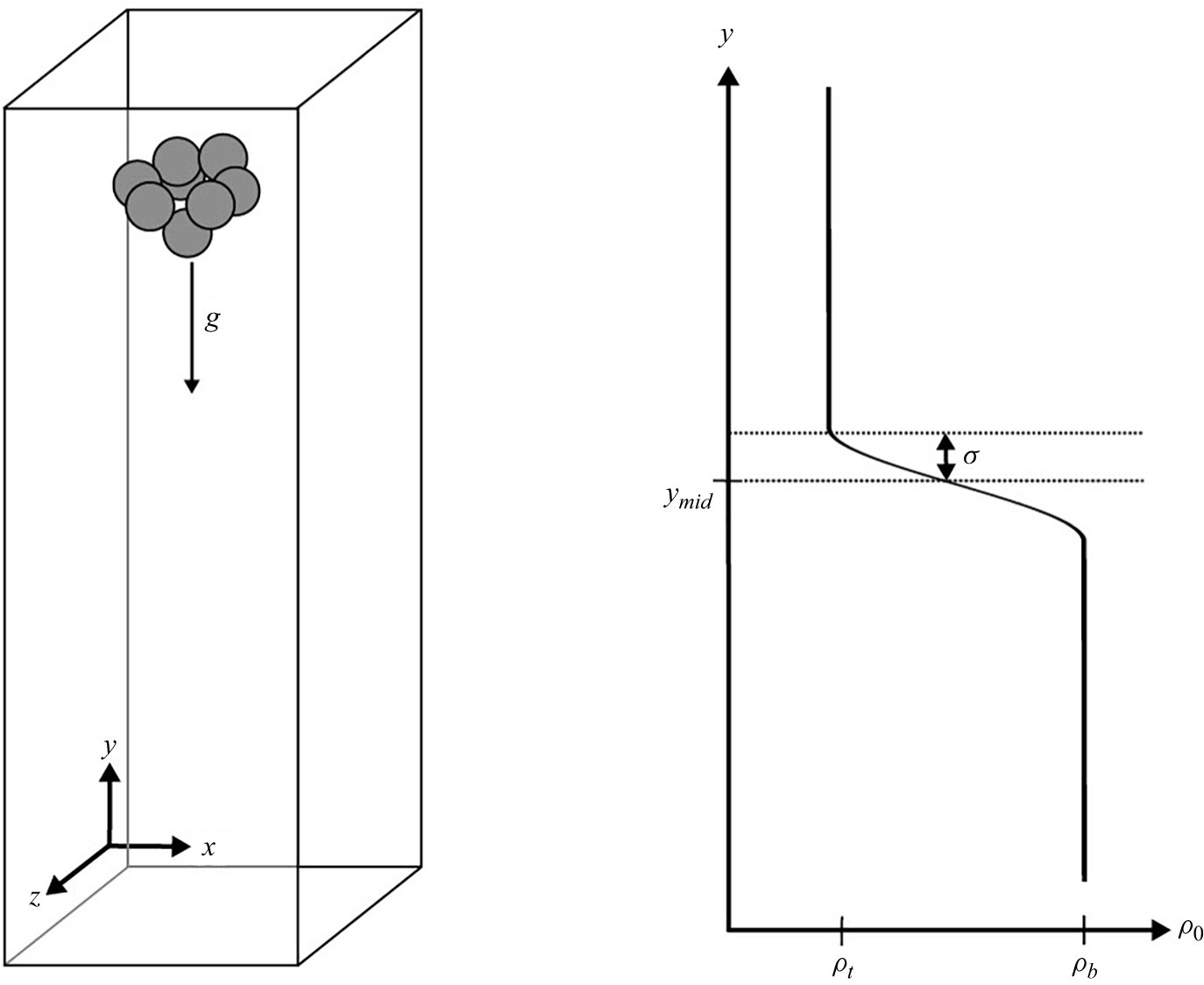

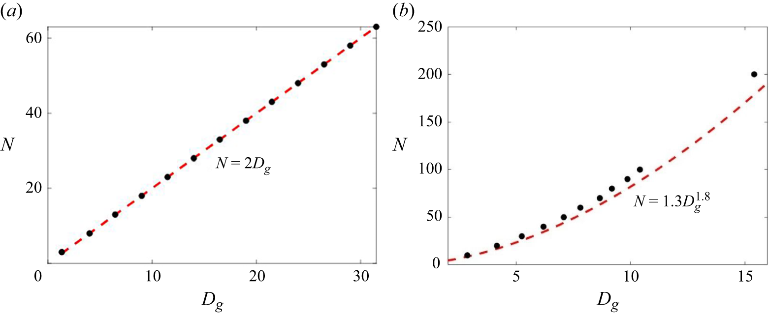


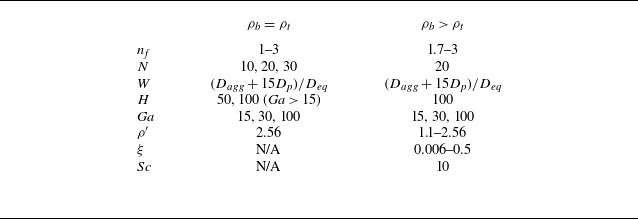


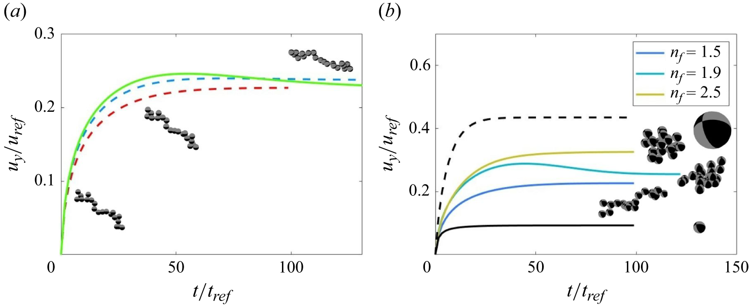


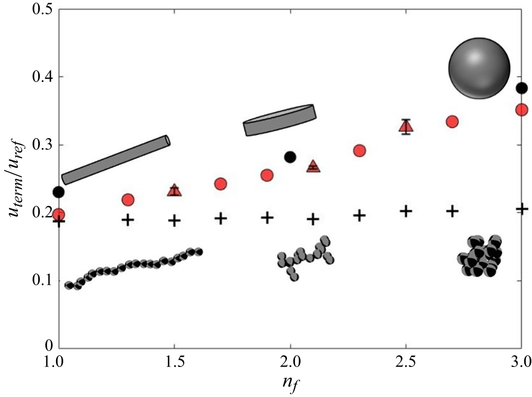


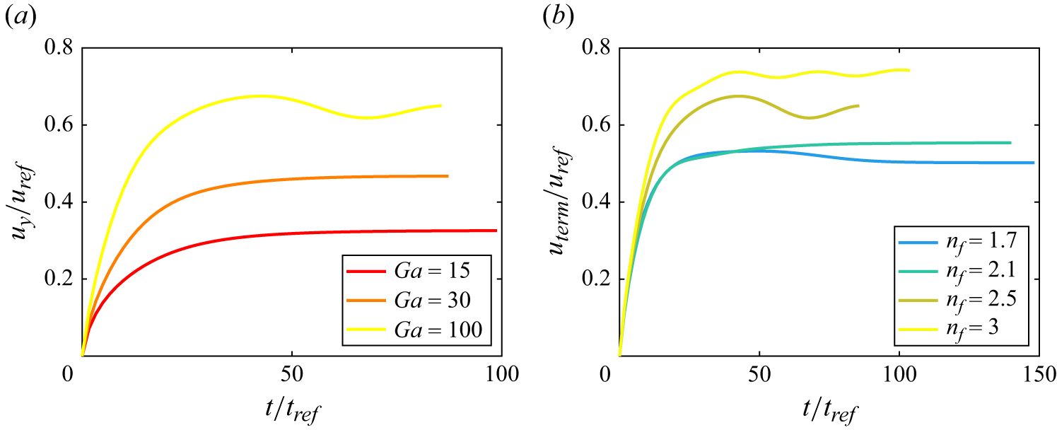


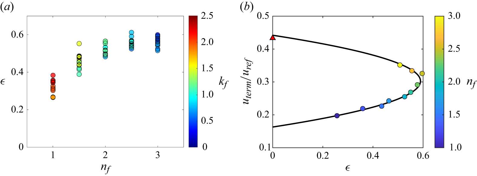


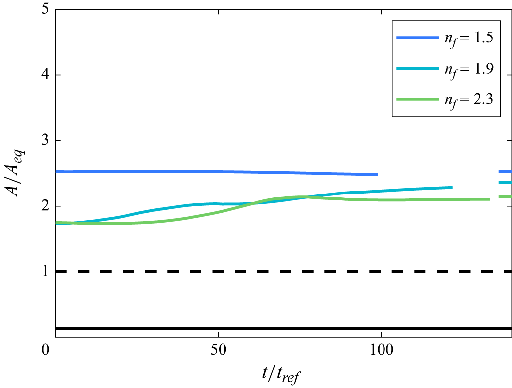


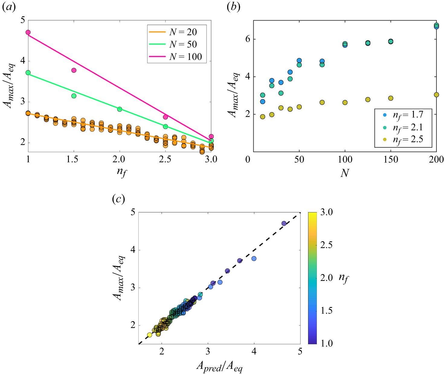


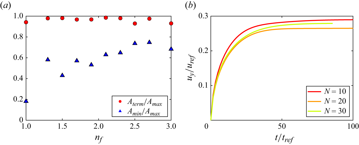


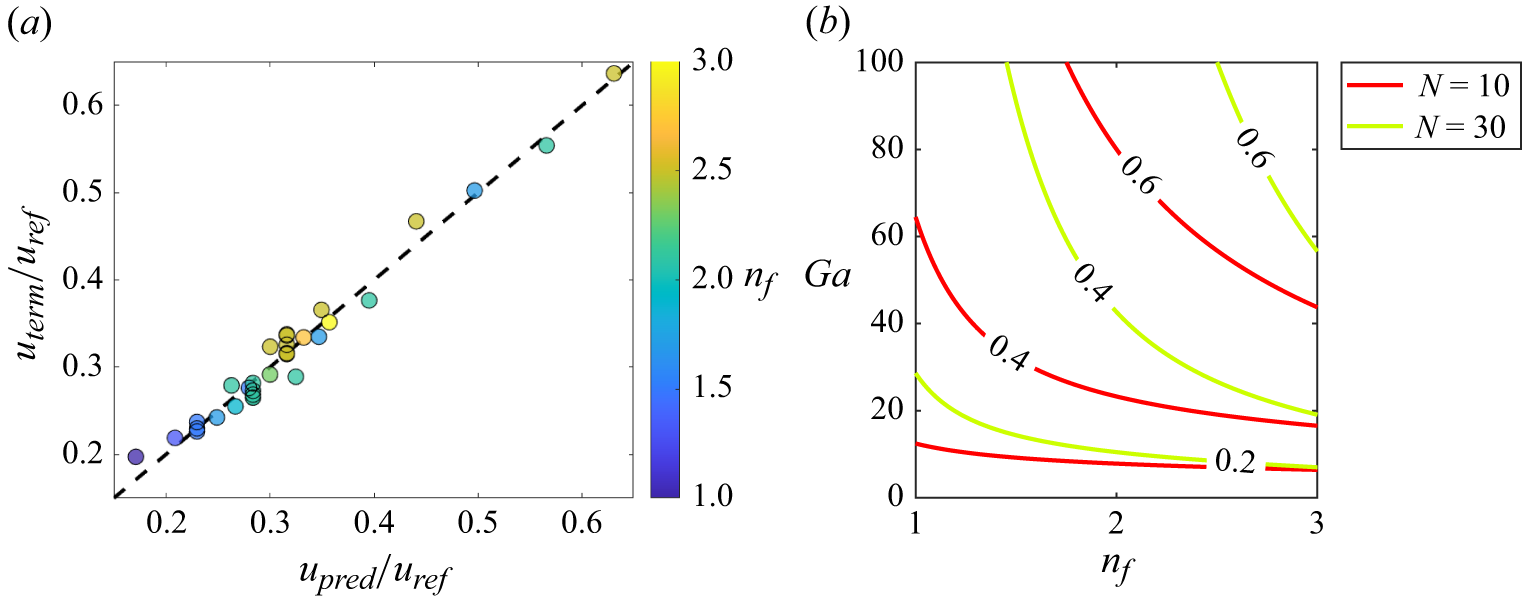


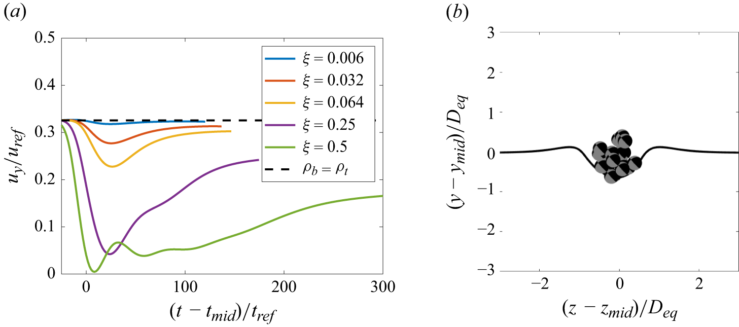


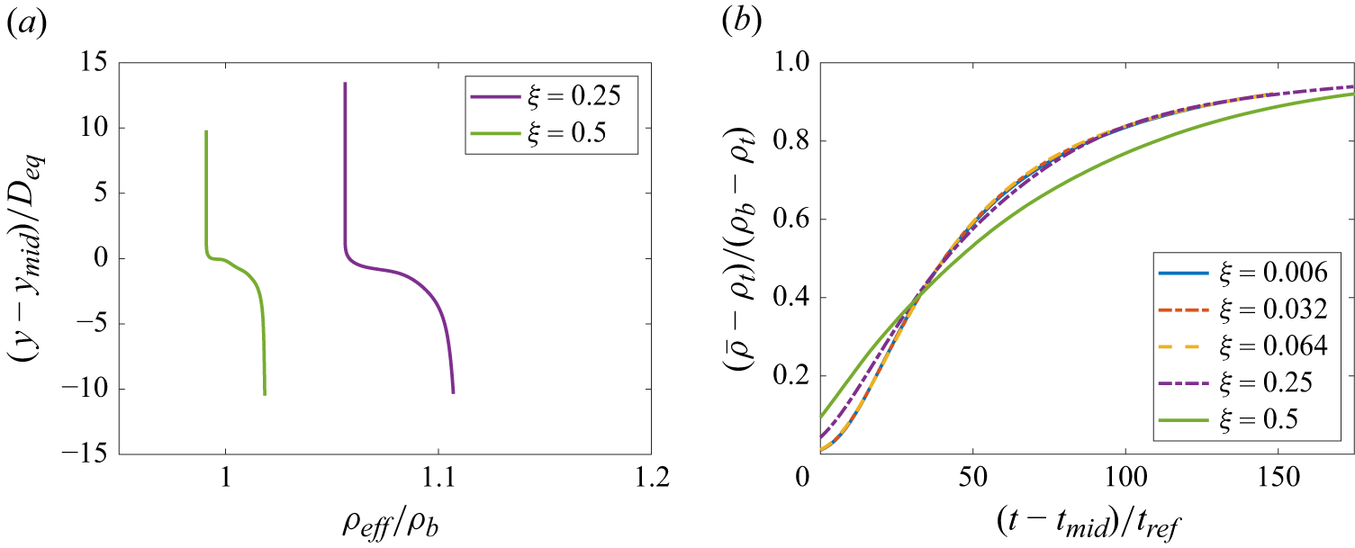


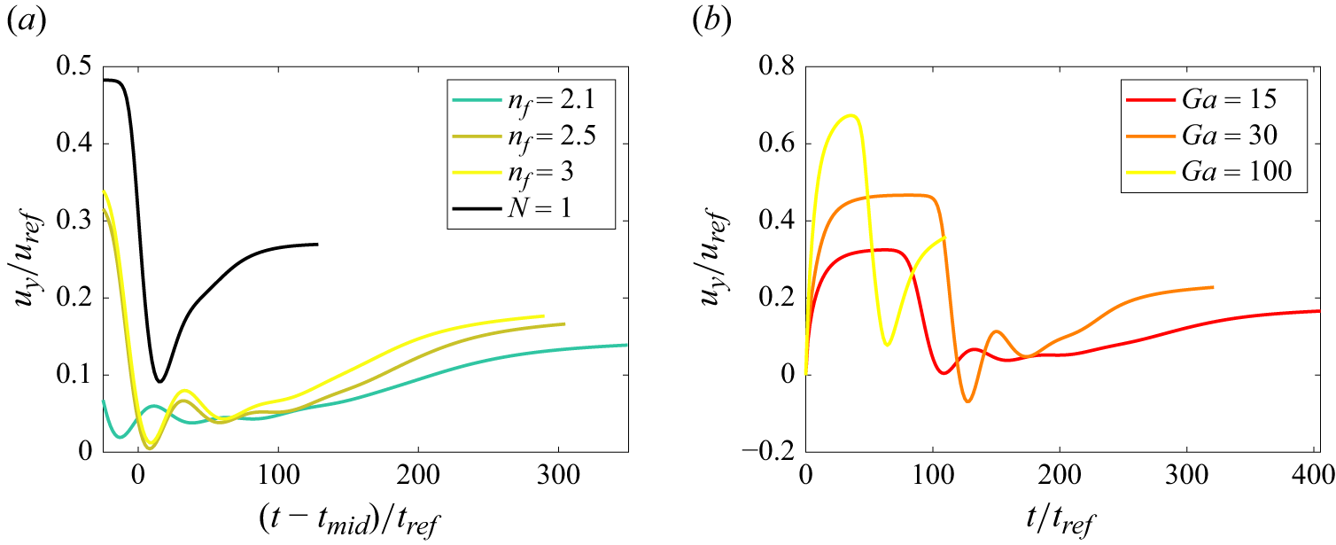


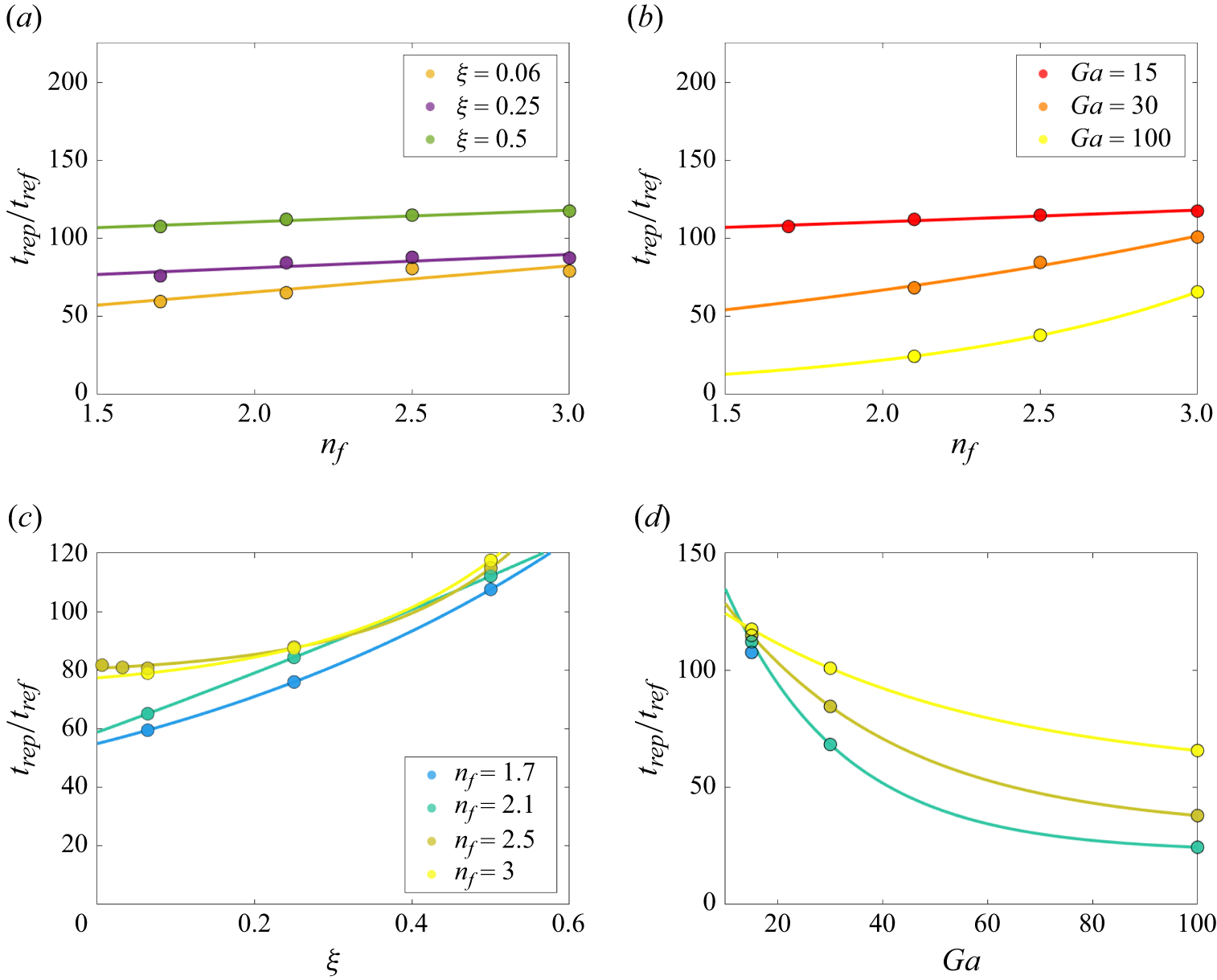


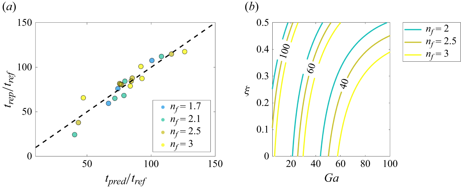


 Open access

