





1 Introduction
The development of chirped pulse amplification (CPA) has enabled the construction of laser systems that deliver ultrashort pulses with peak powers reaching the petawatt (PW) level[
Reference Danson, Haefner, Bromage, Butcher, Chanteloup, Chowdhury, Galvanauskas, Gizzi, Hein, Hillier, Hopps, Kato, Khazanov, Kodama, Korn, Li, Li, Limpert, Ma, Nam, Neely, Papadopoulos, Penman, Qian, Rocca, Shaykin, Siders, Spindloe, Szatmári, Raoul, Zhu, Zhu and Zuegel
1
,
Reference Danson, Hillier, Hopps and Neely
2
]. When tightly focused, these pulses can achieve extreme intensities exceeding
${10}^{23}\ \mathrm{W}/{\mathrm{cm}}^2$
 [
Reference Yoon, Kim, Choi, Sung, Lee, Lee and Nam
3
], creating unique opportunities to study laser–matter interactions in the relativistic regime and drive applications such as laser–plasma acceleration[
Reference Mourou, Tajima and Bulanov
4
,
Reference Esarey, Schroeder and Leemans
5
]. Achieving these record intensities is critically dependent on the ability to perfectly focus the laser pulse in both space and time[
Reference Akturk, Gu, Bowlan and Trebino
6
]. However, ultrashort pulses are inherently broadband, and dispersive effects accumulated during amplification and propagation can cause different frequency components to possess different wavefronts[
Reference Akturk, Gu, Bowlan and Trebino
6
,
Reference Jolly, Gobert and Quéré
7
].
[
Reference Yoon, Kim, Choi, Sung, Lee, Lee and Nam
3
], creating unique opportunities to study laser–matter interactions in the relativistic regime and drive applications such as laser–plasma acceleration[
Reference Mourou, Tajima and Bulanov
4
,
Reference Esarey, Schroeder and Leemans
5
]. Achieving these record intensities is critically dependent on the ability to perfectly focus the laser pulse in both space and time[
Reference Akturk, Gu, Bowlan and Trebino
6
]. However, ultrashort pulses are inherently broadband, and dispersive effects accumulated during amplification and propagation can cause different frequency components to possess different wavefronts[
Reference Akturk, Gu, Bowlan and Trebino
6
,
Reference Jolly, Gobert and Quéré
7
].
These effects are known as spatio-temporal couplings (STCs)[ Reference Akturk, Gu, Bowlan and Trebino 6 ]. Common examples include pulse-front tilt (PFT), often caused by misaligned compressor gratings, and pulse-front curvature (PFC), introduced by chromatic lenses[ Reference Jolly, Gobert and Quéré 7 , Reference Bor 8 ]. In many cases, STCs are undesirable as they effectively lengthen the pulse duration at the focus, thereby reducing the peak intensity[ Reference Bourassin-Bouchet, Stephens, de Rossi, Delmotte and Chavel 9 ]. However, in some advanced applications, STCs are deliberately engineered to control the dynamics of the focal spot, such as creating a ‘flying focus’ to guide laser–plasma interactions[ Reference Sainte-Marie, Gobert and Quéré 10 , Reference Froula, Turnbull, Davies, Kessler, Haberberger, Palastro, Bahk, Begishev, Boni, Bucht, Katz and Shaw 11 ]. Whether for elimination or control, the precise characterization of STCs is essential for modern high-power laser science.
A variety of techniques have been developed to measure STCs[ Reference Alonso, Döpp and Jolly 12 ], which can be broadly categorized into two classes.
-
• Some methods rely on spectrally resolved wavefront sensing. Many variations resort to the use of a Shack–Hartmann sensor paired with tunable or narrowband filters, as seen in techniques such as HAMSTER[ Reference Cousin, Bueno, Forget, Austin and Biegert 13 ] or FALCON[ Reference Weisse, Esslinger, Howard, Foerster, Haberstroh, Doyle, Norreys, Schreiber, Karsch and Döpp 14 ]. Single-shot capability is achieved using a dispersive element to measure multiple colours at different positions on the sensor[ Reference Gabolde and Trebino 15 ]. The recently presented RAVEN technique further expands this to vector fields[ Reference Howard, Esslinger, Weiße, Schröder, Eberle, Wang, Karsch, Norreys and Döpp 16 ].
-
• Others are based on spatially-resolved spectroscopy, for example using imaging Fourier-transform spectroscopy (FTS). TERMITES[ Reference Miranda, Kotur, Rudawski, Guo, Harth, L’Huillier and Arnold 17 , Reference Pariente, Gallet, Borot, Gobert and Quéré 18 ] and INSIGHT[ Reference Borot and Quéré 19 ], which build a hyperspectral data cube by scanning a temporal delay, can be seen as examples for this approach.
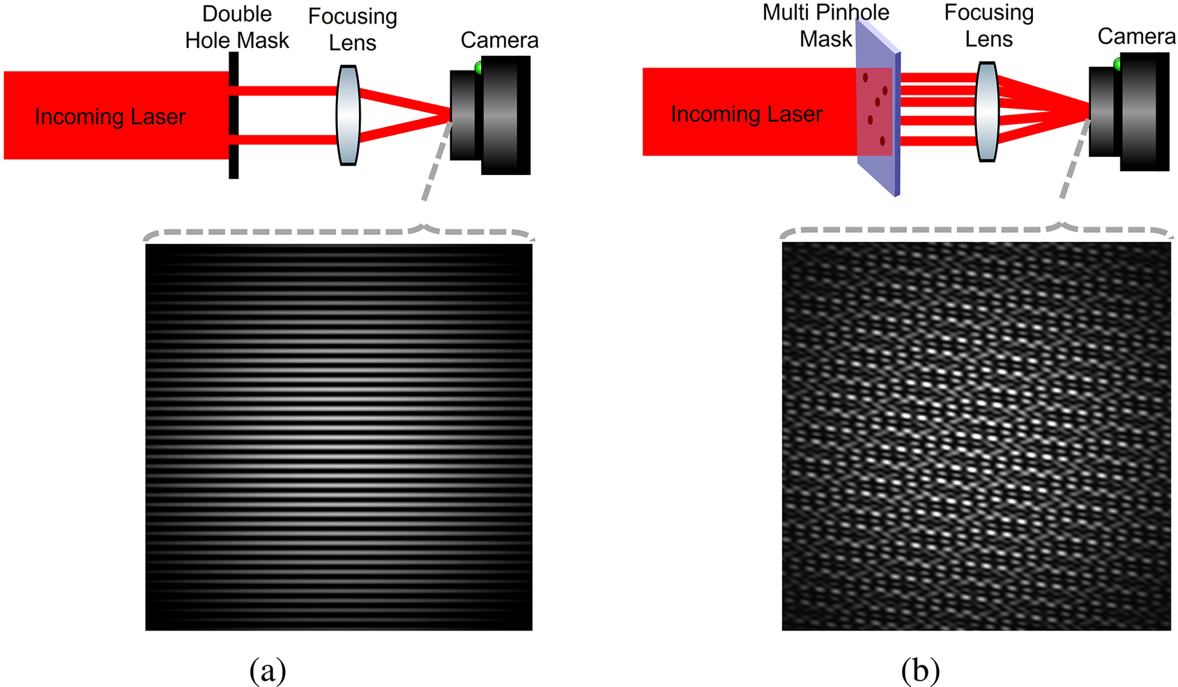
A somewhat orthogonal approach was recently introduced by Smartsev et al. [ Reference Smartsev, Liberman, Andriyash, Cavagna, Flacco, Giaccaglia, Kaur, Monzac, Tata, Vernier, Malka, Lopez-Martens and Faure 20 ]: the IMPALA (Iterative Multispectral Phase Analysis for LAsers) method[ Reference Smartsev, Liberman, Andriyash, Cavagna, Flacco, Giaccaglia, Kaur, Monzac, Tata, Vernier, Malka, Lopez-Martens and Faure 20 ] extends Young’s double-slit interferometry (Figure 1(a)) by using a mask with multiple, aperiodically arranged pinholes in the laser’s near-field (Figure 1(b)). The interference of the resulting beamlets in the far-field creates a complex speckle pattern that encodes the spectrally resolved wavefront. In the original implementation, this information was retrieved using the iterative Gerchberg–Saxton phase retrieval algorithm[ Reference Smartsev, Liberman, Andriyash, Cavagna, Flacco, Giaccaglia, Kaur, Monzac, Tata, Vernier, Malka, Lopez-Martens and Faure 20 ]. The simple setup allows it to be easily integrated into the beamline without adding any additional dispersing optical setups, making it an in situ measurement.
Simplest sketch of the IMPALA setup for a single-colour flat phase laser beam. Also shown are the resulting camera images in the focal plane. It can be seen as an extension to the classical double-slit experiment with holes instead of slits as shown in (a). If there were a phase difference between the beamlets, the fringe pattern would shift by the phase difference. Extending this to five holes with non-regular spacing is shown in (b). The resulting speckle pattern in the focal plane appears chaotic but is in fact the result of a deterministic superposition of individual double pinhole interference patterns.

Figure 1 Long description
The left panel, labeled a, shows a horizontal red incoming laser beam passing through a double hole mask, then a focusing lens, and finally reaching a camera. Below this, a rectangular camera output displays evenly spaced horizontal bright and dark fringes. The right panel, labeled b, shows a similar setup but with a multi pinhole mask containing five non-uniformly spaced holes. The laser passes through this mask, then a focusing lens, and reaches a camera. The camera output below shows a dense, irregular speckle pattern. All optical elements are labeled: Incoming Laser, Double Hole Mask or Multi Pinhole Mask, Focusing Lens, and Camera. Dashed lines connect each camera to its respective output image, indicating the correspondence between the optical setup and the resulting interference pattern.
In this paper, we present a new interpretation and a deterministic retrieval algorithm for the setup used for the IMPALA method. Instead of relying on iterative phase retrieval, which might not converge to the correct result, we develop a direct linear forward model based on the theory of multi-beamlet interference in the Fourier domain. This approach allows for a direct, non-iterative reconstruction of the spatio-spectral phase, which is not only computationally faster and more robust but also allows for the propagation of measurement uncertainties. We demonstrate this technique with a single-shot measurement of the ATLAS-3000 PW laser. In our implementation, the pinhole mask serves the dual purpose of creating the required speckle pattern while simultaneously attenuating the full-energy beam, providing a minimal and robust diagnostic. Note that this is an ideal attenuator, as no additional phase is introduced into the transmitted beamlets.
2 Theory
The interference of the focused beamlets can be understood by calculating the field in the focal plane of the focusing optic. As the whole theory can be derived analytically, in parallel, every plane was also simulated in order to verify the formalism as well as to optimize and test the mask design. The general way to calculate the far-field of a focusing optic is given by the Fraunhofer diffraction:

Here,
$\vec{r}$
 is the lateral position vector in the focal plane,
$f$
is the lateral position vector in the focal plane,
$f$
 is the focal length,
$\lambda$
is the focal length,
$\lambda$
 is the wavelength with corresponding wave number
$k$
is the wavelength with corresponding wave number
$k$
 and
${E}_{\mathrm{near}\hbox{-} \mathrm{field}}$
and
${E}_{\mathrm{near}\hbox{-} \mathrm{field}}$
 is the initial electric near-field. For simplicity, it is assumed that the field is linearly polarized. Explicitly writing the Fourier integral gives the following:

where
${\vec{r}}_0$
 denotes the lateral position in the near-field. In the case of a mask with infinitely small pinholes, the integral becomes a summation over those holes where the field amplitude is
${E}_m$
denotes the lateral position in the near-field. In the case of a mask with infinitely small pinholes, the integral becomes a summation over those holes where the field amplitude is
${E}_m$
 , and the phase is
${\varphi}_m$
, and the phase is
${\varphi}_m$
 :
:

Here,
${\vec{k}}_m=\frac{k}{f}\left(\begin{array}{@{}c@{}}{x}_m\\ {}{y}_m\end{array}\right)$
 is the wave vector projected onto the focal plane. As a result, the field in the focal plane can be seen as the interference of
$N$
is the wave vector projected onto the focal plane. As a result, the field in the focal plane can be seen as the interference of
$N$
 plane waves, where
$N$
plane waves, where
$N$
 is the number of pinholes.
2.1 Plane wave interference
The individual plane waves are now given by the following:

where the prefactor of the summation has been included in
${E}_m$
 . The intensity of an arbitrary field is given by
${I=\frac{\epsilon_0c}{2}{\epsilon}_0\vec{E}\cdot {\vec{E}}^{\ast }}$
. The intensity of an arbitrary field is given by
${I=\frac{\epsilon_0c}{2}{\epsilon}_0\vec{E}\cdot {\vec{E}}^{\ast }}$
 . For the intensity of the interference field
${{E}_{mn}={E}_m+{E}_n}$
. For the intensity of the interference field
${{E}_{mn}={E}_m+{E}_n}$
 we obtain the following:

In Fourier space this expression results in three distinguished peaks (
$\delta$
 -functions):

The latter two terms are the interference terms, which are complex due to the phase shift
$\Delta {\varphi}_{nm}={\varphi}_n-{\varphi}_m$
 between the waves. Furthermore, the position of these peaks is solely determined by the difference of the wave vectors
$\Delta {\vec{k}_{nm}}={\vec{k}}_n-{\vec{k}_{\!m}}$
between the waves. Furthermore, the position of these peaks is solely determined by the difference of the wave vectors
$\Delta {\vec{k}_{nm}}={\vec{k}}_n-{\vec{k}_{\!m}}$
 . As the longitudinal (
$z$
. As the longitudinal (
$z$
 ) component is identical for both, this is simply the distance vector between the pinhole positions in wave numbers. If we denote the positions of the pinholes as
$\left({x}_m,{y}_m\right)$
) component is identical for both, this is simply the distance vector between the pinhole positions in wave numbers. If we denote the positions of the pinholes as
$\left({x}_m,{y}_m\right)$
 and
$\left({x}_n,{y}_n\right)$
and
$\left({x}_n,{y}_n\right)$
 , then the vector
$\Delta {\vec{k}}_{nm}$
, then the vector
$\Delta {\vec{k}}_{nm}$
 can be written as follows:

where
$\lambda$
 is the wavelength of the light used in the experiment and f is the focal length of the focusing optic.
We can easily extend this result to multi-beam interference, where the intensity is given as the sum of all combinations of interferences. When considering
$N$
 beams, the total electric field will be
$\vec{E}={\sum}_{m=1}^N{E}_m{e}^{i\left(\omega t-{\vec{k}}_m\cdot \vec{r}+{\varphi}_m\right)}$
beams, the total electric field will be
$\vec{E}={\sum}_{m=1}^N{E}_m{e}^{i\left(\omega t-{\vec{k}}_m\cdot \vec{r}+{\varphi}_m\right)}$
 . This results in an intensity of

In Fourier space we can now see the pattern described above with a little modification:

For
$n=m$
 we again identify the real part
${E}_n^2$
we again identify the real part
${E}_n^2$
 , because
${\vec{k}}_{nn}=0=\Delta {\varphi}_{nn}$
, because
${\vec{k}}_{nn}=0=\Delta {\varphi}_{nn}$
 . For switching
$n$
. For switching
$n$
 with
$m$
with
$m$
 we can verify with
${\vec{k}}_{nm}=-{\vec{k}}_{mn}$
we can verify with
${\vec{k}}_{nm}=-{\vec{k}}_{mn}$
 as well as
$\Delta {\varphi}_{nm}=-\Delta {\varphi}_{mn}$
as well as
$\Delta {\varphi}_{nm}=-\Delta {\varphi}_{mn}$
 that the form of our two complex terms is again given.
Assuming the problem is spatially sparse and can be sufficiently separated into parts that do not overlap, we can isolate the terms, that is

From here we can take the argument and log-absolute values to obtain the phase difference and the field amplitude:


This result implies that we can evaluate the Fourier transform of the interference pattern and retrieve a signal that is directly related to the phase and amplitude of the interfering plane waves.
2.2 Modelling the imaging system
In practice, the interfering waves will have an intensity distribution that is determined by the pinhole shape and the focusing optics. For circular pinholes, the far-field intensity pattern takes the form of an Airy pattern, whose Fourier transformation is again circular. However, we do not deal with perfect imaging systems and the Fourier space expression above has thus to be modified. This can be achieved by convolving the previous equations with the shape of the pinholes, the point spread function (PSF) of the optical system and the PSF of the detector range. Most generally, we can use a function
$f\left(\xi \right)$
 instead of
$\delta \left(\xi \right)$
instead of
$\delta \left(\xi \right)$
 to take this form factor into account. The important consequence of the form factor is that the clear spatial separation of features that we relied on so far disappears, at least to some extent. Consider two interference points
$\Delta {\vec{k}}_{nm}$
to take this form factor into account. The important consequence of the form factor is that the clear spatial separation of features that we relied on so far disappears, at least to some extent. Consider two interference points
$\Delta {\vec{k}}_{nm}$
 and
$\Delta {\vec{k}}_{ij}$
and
$\Delta {\vec{k}}_{ij}$
 whose distance in Fourier space
$\parallel \Delta {\vec{k}}_{nm}-\Delta {\vec{k}}_{ij}\parallel$
whose distance in Fourier space
$\parallel \Delta {\vec{k}}_{nm}-\Delta {\vec{k}}_{ij}\parallel$
 is within the extent of the form factor. In this case,

contains contributions from both interferences that add up. Now we cannot perform the same simple separations to retrieve phase and amplitude. One solution to this problem is to only consider points in the retrieval that are clearly separated and discard those that overlap. One can also try reducing the extent of
$f\left(\xi \right)$
 , for example by using smaller pinholes in the mask or using a deconvolution with the known form factor. With the simplest approximation, we can think of
$f\left(\xi \right)$
, for example by using smaller pinholes in the mask or using a deconvolution with the known form factor. With the simplest approximation, we can think of
$f\left(\xi \right)$
 being a Gaussian distribution centred around
${\vec{k}}_{nm}$
being a Gaussian distribution centred around
${\vec{k}}_{nm}$
 . The standard deviation is determined by the properties of the optical setup:
${\sigma}^2\approx \frac{A^2}{{\left(0.84\lambda f\right)}^2}+\frac{1}{D^2}$
. The standard deviation is determined by the properties of the optical setup:
${\sigma}^2\approx \frac{A^2}{{\left(0.84\lambda f\right)}^2}+\frac{1}{D^2}$
 , where
$A$
, where
$A$
 is the pinhole size,
$D$
is the pinhole size,
$D$
 is the size of the imaging detector and
$0.84$
is the size of the imaging detector and
$0.84$
 comes from approximating the Airy pattern with a Gaussian distribution[
Reference Zhang, Zerubia and Olivo-Marin
21
]. With this, it is already clear that reducing the pinhole size will be effective only up to a limit of
$A\approx \frac{0.84\lambda f}{D}$
comes from approximating the Airy pattern with a Gaussian distribution[
Reference Zhang, Zerubia and Olivo-Marin
21
]. With this, it is already clear that reducing the pinhole size will be effective only up to a limit of
$A\approx \frac{0.84\lambda f}{D}$
 . From then on, the positive effect of reducing the pinhole size is on a smaller scale. In addition, one would also have to consider the non-perfect imaging in the form factor, for example due to the finite size of any focusing optic.
2.3 Broadband sources
So far, only the case of one wavelength has been considered. Ultrashort lasers have a broadband spectrum, meaning that
$\vec{\Delta}{k}_{nm}$
 as well as
${E}_{m,n}$
as well as
${E}_{m,n}$
 and
$\Delta{\varphi}_{nm}$
and
$\Delta{\varphi}_{nm}$
 depends on
$\lambda$
depends on
$\lambda$
 . Hence, one must integrate over it:

The main consequence is that for broadband sources, streaks are observed, rather than single diffracted points. This acts like the dispersion by a prism or grating and therefore allows direct access to the spectrally resolved phase differences and amplitude products. However, a superposition of streaks at different frequencies is now also possible, which must be considered regarding the separability of amplitude and phase. While the phase part could be linearized using the assumption of a slowly varying phase, the amplitude cannot be easily separated. Therefore, streak overlap should be excluded as much as possible by the mask design.
3 Retrieval
The theory discussed in the previous section can be used to set up a forward model of the measurement process, which we can then use to retrieve information from experiments.
3.1 Phase retrieval
Retrieving the phase differences is in principle as simple as Equation (11) indicates under the assumption that there is no overlap between streaks from different pinhole pairs, as discussed in the previous section. However, there is one additional condition that must be fulfilled, and that is the intra-streak overlap. As the intensity is measured in the far-field on a finite, pixelated detector, we also only obtained a finite, discrete FT, in practice. Hence, we cannot measure the phase differences depending on the wavelength continuously, but instead have to probe for discrete values/pixels that integrate the field over their size. Hence, it is necessary that
${E}_n{E}_m$
 and
$\Delta {\varphi}_{mn}$
and
$\Delta {\varphi}_{mn}$
 vary slowly in this range for broadband sources. This condition is usually ensured by the fact that we observe focusable, propagating laser pulses rather than arbitrary electric fields. Note that as the streaks scale with the distance between pinholes, longer streaks also obtain more measurable data points; hence, for those, we can achieve a higher spectral resolution.
3.2 Phase unwrapping
For the following derivations, we assume that we have obtained the phase difference values
$\Delta {\varphi}_{nm}$
 for discrete wavelengths and neglect the finite resolution of the sensor. Any phase value has the problem that it is only unique within the interval
$\left[0,2\pi \right)$
for discrete wavelengths and neglect the finite resolution of the sensor. Any phase value has the problem that it is only unique within the interval
$\left[0,2\pi \right)$
 or equally
$\left[-\pi, \pi \right)$
or equally
$\left[-\pi, \pi \right)$
 and otherwise will be wrapped. For a large beam, this is a plausible case, especially since negative values are also possible, thereby reducing the range of absolute values to
$\pi$
and otherwise will be wrapped. For a large beam, this is a plausible case, especially since negative values are also possible, thereby reducing the range of absolute values to
$\pi$
 . Hence, one has to make sure that whenever such a phase wrapping occurs, it is detected and corrected for. This can be achieved by using the abundance of phase difference measurements compared to the number of pinholes. Given
$N$
. Hence, one has to make sure that whenever such a phase wrapping occurs, it is detected and corrected for. This can be achieved by using the abundance of phase difference measurements compared to the number of pinholes. Given
$N$
 pinholes, there will be
$N\cdot \left(N-1\right)/2$
pinholes, there will be
$N\cdot \left(N-1\right)/2$
 individual pinhole combinations, as these are the triangle numbers. In total, there are
$N\cdot \left(N-1\right)$
individual pinhole combinations, as these are the triangle numbers. In total, there are
$N\cdot \left(N-1\right)$
 streaks in the Fourier domain due to the indistinguishability of their orientation.
As there is no absolute phase as a reference, one has to make the assumption that the pinholes in proximity to each other on the mask do not have an absolute phase difference larger than
$\pi$
 (to ensure uniqueness of positive and negative values). From the closer pinholes, we can then deduce if pinholes further apart have wrapped the phase or not by using the additivity of the phase difference values:

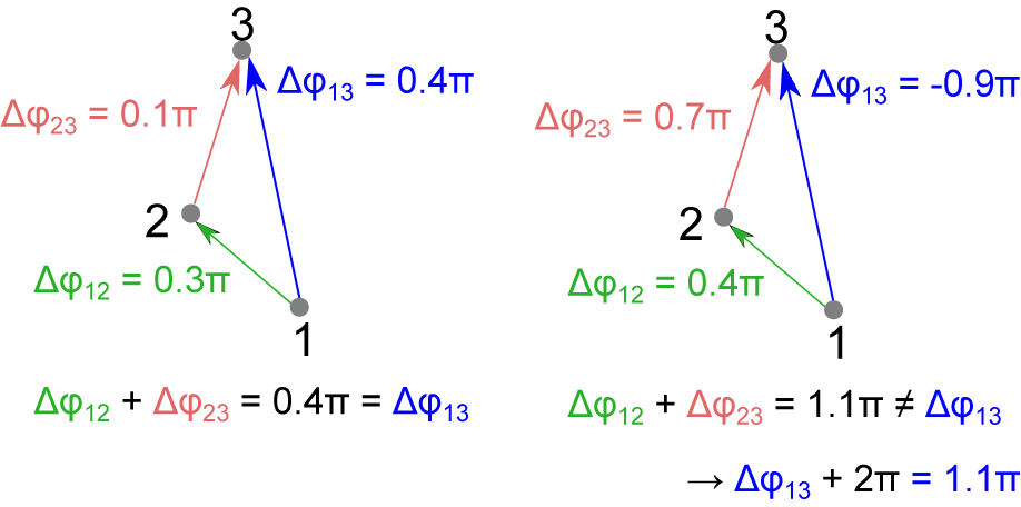
This is easier to understand using an example: consider three pinholes as shown in Figure 2. Pinholes 1 and 2 are the closest, and 2 and 3 are the second closest, whilst 1 and 3 are the furthest apart. In theory, the obtained phase differences of pinholes 1–2 and 2–3 should add up to give the value of 1–3. If this is not the case, one can check which multiple of
$2\pi$
 has to be added to achieve the best match. Of course, for error-free measurements, this is a trivial task and does not provide additional insights; however, in the presence of measurement uncertainties, it will never result in a perfect match and small deviations from a perfect
$2\pi$
has to be added to achieve the best match. Of course, for error-free measurements, this is a trivial task and does not provide additional insights; however, in the presence of measurement uncertainties, it will never result in a perfect match and small deviations from a perfect
$2\pi$
 wrapping will occur. If this is taken into account and also near-perfect matches are allowed and correct with a factor of
$2\pi$
wrapping will occur. If this is taken into account and also near-perfect matches are allowed and correct with a factor of
$2\pi$
 , more measurements can be included in the evaluation to reduce the reconstruction uncertainty. Extending this check to all pinhole combinations yields a net of connected measurements that allows for deducing the unwrapped phase differences for all pairwise pinhole interferences.
Examples for the phase difference matching test for three pinholes using the phase wrapping of
$\Delta \varphi \in \left[-\pi, \pi \right)$
 . In the left-hand example, it checks out, whereas in the right-hand one, it does not, and a correcting factor of
$1\times 2\pi$
. In the left-hand example, it checks out, whereas in the right-hand one, it does not, and a correcting factor of
$1\times 2\pi$
 has to be taken into account.

Figure 2 Long description
There are two panels, left and right, each showing three numbered nodes arranged in a triangle labeled 1 at the bottom, 2 to the upper left, and 3 at the top. In both panels, arrows connect the nodes, each labeled with a phase difference. In the left panel, the arrow from 1 to 2 is green and labeled Delta phi one two equals zero point three pi, the arrow from 2 to 3 is red and labeled Delta phi two three equals zero point one pi, and the arrow from 1 to 3 is blue and labeled Delta phi one three equals zero point four pi. Below the triangle, the equation Delta phi one two plus Delta phi two three equals zero point four pi equals Delta phi one three is shown in green, red, and blue, indicating the corresponding arrows. In the right panel, the arrow from 1 to 2 is green and labeled Delta phi one two equals zero point four pi, the arrow from 2 to 3 is red and labeled Delta phi two three equals zero point seven pi, and the arrow from 1 to 3 is blue and labeled Delta phi one three equals negative zero point nine pi. Below, the equation Delta phi one two plus Delta phi two three equals one point one pi not equal to Delta phi one three is shown in green, red, and blue, with an additional equation indicating Delta phi one three plus two pi equals one point one pi, showing the need for a phase correction.
3.3 Reconstruction of the phase map from phase differences
The phase values
${\varphi}_n$
 can easily be calculated, as they are related to the differences by
$\Delta {\varphi}_{nm}={\varphi}_n-{\varphi}_m$
can easily be calculated, as they are related to the differences by
$\Delta {\varphi}_{nm}={\varphi}_n-{\varphi}_m$
 . Without measurement uncertainty and other sources of errors, the approach in the previous section should allow for the direct deduction of the individual phase values for each pinhole. As there are more phase differences measured than the number of pinholes, the system is overdetermined, and most of them are only required to verify the final result. However, in the presence of measurement noise, these additional measurements allow for a least-squares solution of the problem: combining all
$\Delta {\varphi}_{nm}$
. Without measurement uncertainty and other sources of errors, the approach in the previous section should allow for the direct deduction of the individual phase values for each pinhole. As there are more phase differences measured than the number of pinholes, the system is overdetermined, and most of them are only required to verify the final result. However, in the presence of measurement noise, these additional measurements allow for a least-squares solution of the problem: combining all
$\Delta {\varphi}_{nm}$
 and all
${\varphi}_n$
and all
${\varphi}_n$
 into two vectors
$\mathtt{\varDelta}\varphi$
into two vectors
$\mathtt{\varDelta}\varphi$
 and
$\varphi$
and
$\varphi$
 , respectively, the relation between the phase values and phase differences can be expressed as a linear algebra problem:

Each row of
$\mathbf{R}$
 represents the subtraction of a pair of phase values. For an exemplary case of three pinholes, the matrix
$\mathbf{R}$
represents the subtraction of a pair of phase values. For an exemplary case of three pinholes, the matrix
$\mathbf{R}$
 is defined as follows:

As long as the overlap is sparse, this equation system is overdetermined, and a matrix inversion is not possible. Yet, with the pseudo-inverse
${\mathbf{R}}^{+}$
 the solution having a minimal root mean squared error (RMSE) can be found:

This way of retrieving the phase values in the near-field has a particularly neat side effect: one can leave out any number of phase differences as long as there are still more than the number of phase values to be reconstructed (the matrix stays overdetermined). Of course, the reconstruction accuracy decreases when doing this. On the other hand, it has the advantage that one could fit more pinholes on the mask, such that it becomes unavoidable that some streaks in the FT of the intensity in the focal plane overlap. As long as this affects only a limited number of streaks, one can just ignore those in the reconstruction, such that with the remaining streaks a full reconstruction is still possible.
3.3.1 Propagation of errors
As each value
$\Delta {\varphi}_{nm}$
 is affected by an individual error, it is advantageous for the reconstruction accuracy to extract as many phase differences as possible. However, the linear equation systems allow us to estimate the actual uncertainty on the reconstructed phases. The uncertainty on the measured phase values can be estimated by taking multiple images of the intensity in the focal plane in a short time span, in order to assume that the laser beam parameters are constant for all images. One can then estimate the uncertainty accordingly by comparing the resulting phase differences for each image. The result is a diagonal covariance matrix
${\Sigma}_{\Delta \varphi}^2$
is affected by an individual error, it is advantageous for the reconstruction accuracy to extract as many phase differences as possible. However, the linear equation systems allow us to estimate the actual uncertainty on the reconstructed phases. The uncertainty on the measured phase values can be estimated by taking multiple images of the intensity in the focal plane in a short time span, in order to assume that the laser beam parameters are constant for all images. One can then estimate the uncertainty accordingly by comparing the resulting phase differences for each image. The result is a diagonal covariance matrix
${\Sigma}_{\Delta \varphi}^2$
 . The corresponding covariance matrix for the phase map
${\Sigma}_{\varphi}^2$
. The corresponding covariance matrix for the phase map
${\Sigma}_{\varphi}^2$
 can then be estimated via the following:

3.3.2 Modal fitting
In principle, one can stop here; however one can also fit a modal base to the reconstructed phases, which allows for interpreting the result in a physically easier way as well as estimating the phase map for the full beam. If fewer modes are reconstructed than measurements, this further reduces the influence of noise. A particularly suitable base for fitting the wavefront and STCs combined is the Zernike–Taylor base as introduced in Ref. [Reference Weisse, Esslinger, Howard, Foerster, Haberstroh, Doyle, Norreys, Schreiber, Karsch and Döpp14] and demonstrated in Refs. [Reference Howard, Esslinger, Weiße, Schröder, Eberle, Wang, Karsch, Norreys and Döpp16,Reference Esslinger, Weiße, Eberle, Schröder, Howard, Norreys, Karsch and Döpp22]. This set of basis functions combines the Zernike polynomials for fitting the wavefront component with the Taylor expansion for the spectral phase component. The modes are defined as follows:

Here,
${a}_{m,n}^i$
 are the Zernike–Taylor coefficients to be reconstructed and
${Z}_n^m$
are the Zernike–Taylor coefficients to be reconstructed and
${Z}_n^m$
 are the Zernike polynomials. In order to obtain the
${a}_{m,n}^i$
are the Zernike polynomials. In order to obtain the
${a}_{m,n}^i$
 , another matrix can be set up that links these coefficients to the phase values as shown for phase gradients in Ref. [Reference Weisse, Esslinger, Howard, Foerster, Haberstroh, Doyle, Norreys, Schreiber, Karsch and Döpp14]. A pseudo-inverse of the resulting forward matrix can be obtained and then easily integrated in the introduced matrix formalism.
3.4 Reconstruction of the amplitude map
Similar to Equation (16), the matrix formalism for the amplitude is given by the following:

Here, each row of
$\mathbf{T}$
 is the pairwise addition of the logarithm of field amplitudes
${\mathbf{E}}_{\mathrm{near}\hbox{-} \mathrm{field}}$
is the pairwise addition of the logarithm of field amplitudes
${\mathbf{E}}_{\mathrm{near}\hbox{-} \mathrm{field}}$
 in order to obtain the intensity in the Fourier domain of the far-field
${\mathbf{I}}_{\mathrm{far}\hbox{-} \mathrm{field},\mathrm{FT}}$
in order to obtain the intensity in the Fourier domain of the far-field
${\mathbf{I}}_{\mathrm{far}\hbox{-} \mathrm{field},\mathrm{FT}}$
 . Overall, this is more straightforward than the phase, as no wrapping may occur for the amplitude. Again, for three pinholes
$\mathbf{T}$
. Overall, this is more straightforward than the phase, as no wrapping may occur for the amplitude. Again, for three pinholes
$\mathbf{T}$
 would be defined as follows:

4 Experiments
4.1 General considerations
From the previous discussion we have seen that one of the key parameters determining the resolution of the device is the convolution of the signal due to the form factor. It would seem that a smaller pinhole is always better, but in practice we have to be able to resolve it.
The inference pattern at the focus position
$f$
 emerging from at least two beamlets separated by a distance
$d$
emerging from at least two beamlets separated by a distance
$d$
 has a periodicity of
$\lambda f/d$
has a periodicity of
$\lambda f/d$
 and it should be sampled with half that period. For
$f/d=50$
and it should be sampled with half that period. For
$f/d=50$
 and
$\lambda =800$
and
$\lambda =800$
 nm this means the features of the speckle pattern will occur at a periodicity of
$40\;\mu \mathrm{m}$
nm this means the features of the speckle pattern will occur at a periodicity of
$40\;\mu \mathrm{m}$
 and, thus, sampling should occur with
$20\;\mu \mathrm{m}$
and, thus, sampling should occur with
$20\;\mu \mathrm{m}$
 resolution or higher.
Meanwhile, the angle resolution, and thus the ability to resolve the pinholes themselves, is determined by the size of the sensor. The far-field distribution introduced by the pinholes is chromatic and the smallest resolvable angle
${\theta}_{\mathrm{min}}$
 can be estimated by the Rayleigh criterion
${\theta}_{\mathrm{min}}\approx 1.22\lambda /A$
can be estimated by the Rayleigh criterion
${\theta}_{\mathrm{min}}\approx 1.22\lambda /A$
 , where
$A$
, where
$A$
 is the aperture size. To resolve a pinhole with the size of the sensor
$D$
is the aperture size. To resolve a pinhole with the size of the sensor
$D$
 at a focal length
$f$
at a focal length
$f$
 , we require that
${\theta}_{\mathrm{min}}\le D/f$
, we require that
${\theta}_{\mathrm{min}}\le D/f$
 . Substituting the expression for the diffraction limit and rearranging for the largest pinhole size given the wavelength, focal length and sensor size, we get
$A\ge 1.22\lambda f/D$
. Substituting the expression for the diffraction limit and rearranging for the largest pinhole size given the wavelength, focal length and sensor size, we get
$A\ge 1.22\lambda f/D$
 . For 800 nm wavelength with
$f=10$
. For 800 nm wavelength with
$f=10$
 m and a sensor size of
$D=10$
m and a sensor size of
$D=10$
 mm, we get
${A}_{\mathrm{min}}\approx 1$
mm, we get
${A}_{\mathrm{min}}\approx 1$
 mm.
mm.
So we get a minimum resolution
$\Delta x\le \frac{1}{2}\lambda f/d$
 and a minimum sensor size
$D\ge 1.22\lambda f/A$
and a minimum sensor size
$D\ge 1.22\lambda f/A$
 . This translates into a pixel number
${n}_{\mathrm{px}}\ge 2.5d/A$
. This translates into a pixel number
${n}_{\mathrm{px}}\ge 2.5d/A$
 . With a fixed beam size, as well as pixel size and number on the camera, this relationship allows us to determine the ideal magnification (or de-magnification).
4.2 Mask design
An important part of the experimental design is the mask design and how the number and arrangement of pinholes are chosen. As the speckle pattern in the far-field is deterministic, we can directly influence how the far-field and its Fourier transform look. For obvious reasons, a mask containing a regular grid of pinholes or otherwise recurring pattern does not work as streaks in the Fourier domain overlap and a direct, linear retrieval is not possible. The same holds for a completely random arrangement of pinholes. For a small number of pinholes, the chances of a clear separation in the Fourier domain are quite high, but on the other hand one might not cover enough of the original beam. For a larger number, the opposite is the case, and no trade-off might be sufficient.
Therefore, one wants to set certain criteria for the mask to optimize the pinhole pattern for the given number of pinholes. This can be achieved by quantifying the requirements and weighing them appropriately for the setup in order to build a merit function for the mask. If one uses a true random or semi-ordered mask as a starting point, one can move the positions in order to maximize the merit function. In this way, we transform an initial pattern into a pseudo-random pattern. Requirements that need to be considered are as follows.
-
(1) Rather trivial is that for any mask in which the pinholes are within the diameter of the beam.
-
(2) The pinholes should be distributed near-uniformly on the mask in order to create a phase map with a suitable distribution of measured phase values. As an extreme example, it would not be sensible to measure only phase values in the upper half of the beam and none in the lower half.
-
(3) A minimum distance of neighbouring pinholes ensures that the redundancy of information is minimized. Beamlets from neighbouring pinholes typically do not have a large difference in phase and amplitude.
-
(4) For obvious reasons, overlap in the Fourier domain should be minimized. This ensures that the maximum information can be utilized.
-
(5) An even distribution of streaks in the Fourier domain ensures that features in any orientation can be observed. For a large number of pinholes that are evenly distributed in the near-field, this criterion is fulfilled almost automatically.
-
(6) If the number of pinholes is large enough that some overlap in the Fourier domain is unavoidable, one wants to make sure that the lost information affects the reconstruction quality as little as possible. Therefore, one could take the condition number of the inverse matrix in Equation (18) into account.
In addition, it is beneficial to measure as many phase and amplitude values as possible.
4.3 Calibration
For a predesigned, pseudo-random pinhole mask, we can therefore not only simulate the image in the far-field but also know at which positions in the Fourier space we need to extract the phase differences and amplitudes. However, in practice, there will be slight differences; for example, if the mask is not placed perfectly perpendicular to the beam path, then the pinhole pattern is effectively skewed, and therefore the streak positions in the Fourier plane are also skewed. Analogue to this would be a rotation of the mask around the optical axis. There are two ways to resolve this. The first one is of a numerical nature, as one could compute the best affine transform between a simulated streak pattern in the Fourier domain and the measured one. However, if the infrastructure allows for it, a continuous-wave (CW) laser beam that follows the same beam path as the high-power laser pulse to be measured can and should be used as a reference. For this, in the resulting Fourier transform of the far-field intensity, there are only spots instead of streaks, for which it is rather easy to determine their position, for example by using a peak finder or a centre of mass detection. The resulting positions can then be matched to pinhole pairs from the pre-calculated pattern, for example by a linear sum assignment algorithm. From there, we can directly calculate the expected streak pattern, since the position of the other wavelengths directly scales with the ratio of wavelengths
${k=\frac{\lambda_{\mathrm{cw}}}{\lambda }{k}_{\mathrm{cw}}}$
 . This works especially well in this scenario, where there is no additional imaging involved that may introduce aberrations.
4.4 Experimental setup
The ATLAS-3000 laser system is a titanium:sapphire (Ti:Sa) laser and is capable of delivering a maximum pulse energy of 90 J before compression. After compression, the laser pulse duration is 27 fs, placing its peak power in the PW range. After the final expander, the beam diameter measures 27 cm.
For particle acceleration experiments, the system can provide the laser pulse at full energy or, for diagnostic purposes, at much lower energy levels by using a reflective attenuator positioned after the final amplifiers and before the compressor and beam expander. However, the compressor not only scales down the overall laser pulse energy but also alters its spatio-temporal shape. Therefore, the use of the pseudo-random mask is a more elegant solution to attenuate the beam for diagnostics, as the transmitted laser beamlets do not pass any optical element as long as the hole size is large compared to the hole length and the laser wavelength. In addition, in this way it is also shot at full power on the compressor gratings, allowing for the measurement of dynamic effects by compressor heating as well[ Reference Leroux, Eichner and Maier 23 ]. In the conducted experiments, the laser operated at 19.5 J prior to compression.
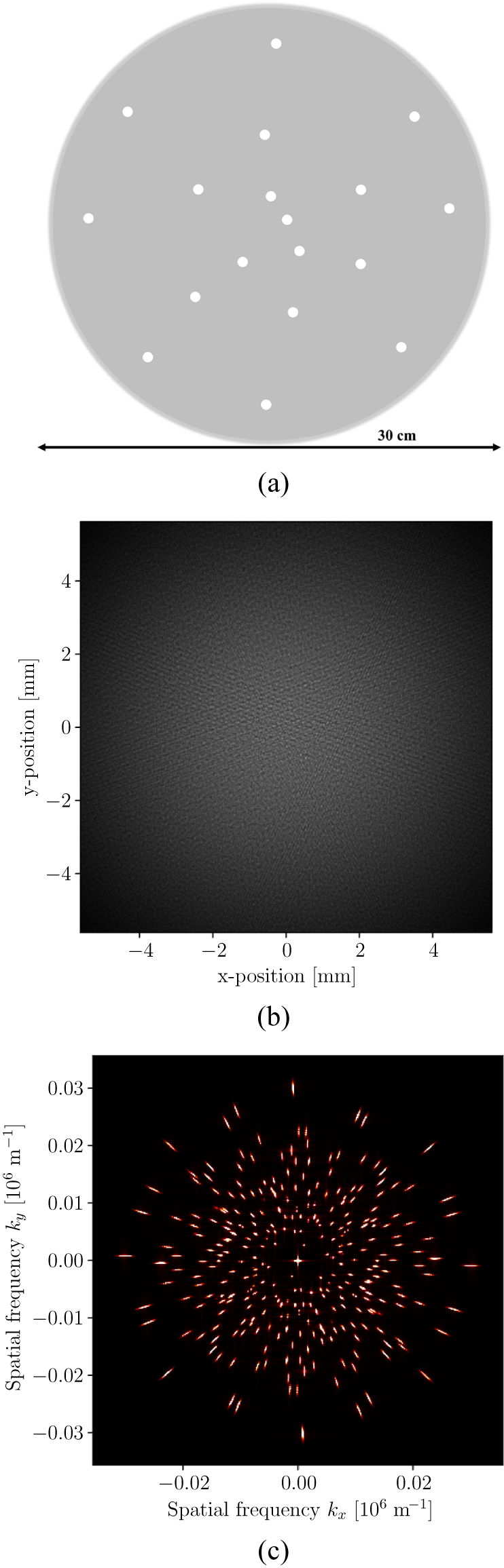
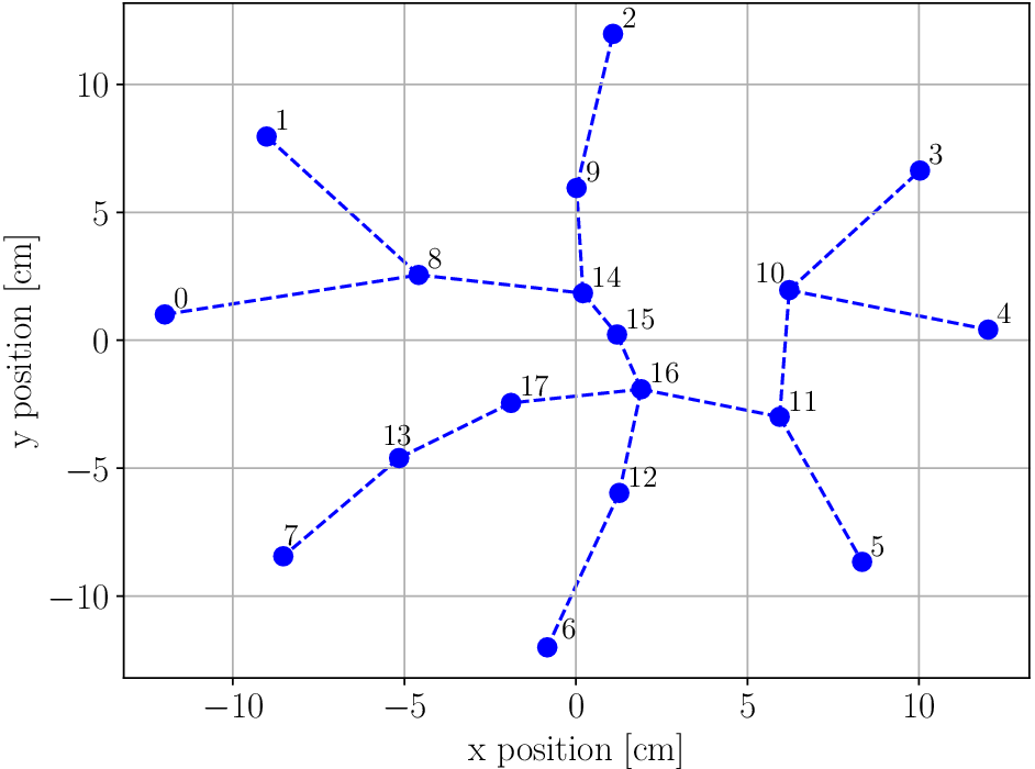
We designed a mask containing 18 holes for the demonstration of our technique. For the optimization of the pseudo-random pinhole pattern, we used the mentioned possible criteria (1)–(5) from Section 4.2. For the chosen amount, full separation of streaks in the Fourier domain is still possible, and hence criterion (6) is not necessary. The beam radius for the maximum size of the pinhole distribution is 28 cm and the size for the pinholes was chosen to be 0.85 mm. The final mask design is shown in Figure 3(a) as well as a simulated focal-plane intensity image in Figure 3(b) and the resulting streak pattern in the Fourier domain in Figure 3(c). The necessary nearest neighbour connections for this mask design for monitoring phase wrapping are shown in Figure 4. The mask was manufactured using laser cutting of anodized AlMg3 with a thickness of 0.5 mm. This material was chosen as its reflection is diffuse, which is beneficial for the experimental operation. As only a small part of the laser energy is transmitted, a significant amount of energy must be deposited. An absorbing material would more likely degrade over time, especially when using a reasonable thickness. However, we cannot reflect it directly back as the reflected pulse could go back through the amplification beamline and damage the laser frontend. In addition, at ATLAS-3000, there is a fast Pockels cell installed to block these back-reflections as well as a diode that monitors them.
(a) Front-view of the final mask design with 18 pinholes. The pinhole size is significantly exaggerated for visibility. (b) Simulated image in the far-field for the flat phase and amplitude and a Gaussian spectrum. (c) Absolute value of the Fourier-transformed far-field intensity.

Figure 3 Long description
Panel a shows a circular gray mask with a diameter of 30 cm. It contains 18 white circular pinholes arranged in a non-uniform, semi-random distribution across the surface. Panel b is a simulated intensity plot on a black background with a fine, grainy texture. The x-axis and y-axis both represent position in millimeters, ranging from minus 4 to 4. Panel c is a Fourier-transformed intensity plot showing a dense radial pattern of bright red and white spots on a black background. The x-axis is labeled Spatial frequency k sub x in units of 10 super 6 m super minus 1, and the y-axis is labeled Spatial frequency k sub y in the same units. Both axes range from minus 0.03 to 0.03. The spots are concentrated around a central bright point and radiate outward in a symmetric, starburst-like pattern.
The phase connections used for checking for phase wrapping.

The mask was installed in the Electron and Thompson Test Facility (ETTF) experimental chamber, which is usually used for laser wakefield acceleration of electrons. There, the mask is placed directly after the first mirror in the vacuum chamber and before an
$f=10\;\mathrm{m}$
 focusing parabola. It is attached to a motorized, retractable mount that allows operation with and without the mask. The mask moved in the beam path was still at a slight angle compared to the optical axis to further mitigate the risk of direct back-reflections.
We installed an additional mirror on a motorized stage about 70 cm before the focal plane in order to image the far-field intensity outside of the acceleration setup. We placed a U3-3992SE-M Rev. 1.2. camera by iDS in the new focal plane. The camera was also mounted on a motorized stage along the optical axis in order to find the focal plane using the attenuated beam with the mask moved out of the beam path.
4.5 Results
After conducting the measurements, we noticed that the mask diameter was set too large. We assumed a beam size of 27 cm and designed a maximum mask diameter of 28 cm. However, by investigating the part of the mask where a small amount of material was ablated, we deduced that the actual beam diameter is about 24 cm, which has not been investigated before in this experimental setup. Therefore, as a perfect alignment of the mask with the centre of the beam is hardly possible, we deduced that the outer pinholes may not have been illuminated properly. Hence, we decided not to use the streaks from pinholes at this radius in the final reconstruction. In addition, another pinhole was located directly in the shadow of a small lever holding a tiny pick-off mirror used for spectral phase reconstruction. Therefore, this pinhole had to be excluded from the reconstruction as well. The final reconstruction will only include nine pinholes in the central region of the mask. Nonetheless, this does not devalidate showcasing the general principle of the setup and the analysis formalism.
The attenuation of the mask is twofold. Firstly, it blocks a large amount of the laser pulse, given by the squared ratio of the diameter of the beam (
${d}_{\mathrm{Beam}}$
 ) and the pinholes (
${d}_{\mathrm{Pinholes}}$
) and the pinholes (
${d}_{\mathrm{Pinholes}}$
 ), times the number of pinholes (
$N$
), times the number of pinholes (
$N$
 ). This intensity reduction
${\chi}_{\mathrm{blocking}}$
). This intensity reduction
${\chi}_{\mathrm{blocking}}$
 is then
$N\cdot {d}_{\mathrm{Pinholes}}^2/{d}_{\mathrm{Beam}}^2$
is then
$N\cdot {d}_{\mathrm{Pinholes}}^2/{d}_{\mathrm{Beam}}^2$
 . In the focal plane, the main size of the area illuminated also scales with the same ratio, leading to the secondary intensity reduction effect. This has to be scaled again by the number of pinholes, which incorporates the possibly constructive interference of the beamlets. This intensity reduction is hence given as well by
${\chi}_{\mathrm{spreading}}=N\cdot {d}_{\mathrm{Pinholes}}^2/{d}_{\mathrm{Beam}}^2$
. In the focal plane, the main size of the area illuminated also scales with the same ratio, leading to the secondary intensity reduction effect. This has to be scaled again by the number of pinholes, which incorporates the possibly constructive interference of the beamlets. This intensity reduction is hence given as well by
${\chi}_{\mathrm{spreading}}=N\cdot {d}_{\mathrm{Pinholes}}^2/{d}_{\mathrm{Beam}}^2$
 . The total intensity reduction is hence
${\chi}_{\mathrm{total}}={\chi}_{\mathrm{blocking}}\cdot {\chi}_{\mathrm{spreading}}={N}^2\cdot {d}_{\mathrm{Pinholes}}^4/{d}_{\mathrm{Beam}}^4$
. The total intensity reduction is hence
${\chi}_{\mathrm{total}}={\chi}_{\mathrm{blocking}}\cdot {\chi}_{\mathrm{spreading}}={N}^2\cdot {d}_{\mathrm{Pinholes}}^4/{d}_{\mathrm{Beam}}^4$
 . In our scenario, this leads to a reduction of about
$5\times {10}^8$
. In our scenario, this leads to a reduction of about
$5\times {10}^8$
 . Together with an ND-8 filter placed in front of the camera, this led to a total reduction of about
$5\times {10}^{16}$
. Together with an ND-8 filter placed in front of the camera, this led to a total reduction of about
$5\times {10}^{16}$
 , enough to bring the original intensity of about
$5\times {10}^{19}\ \mathrm{W}/{\mathrm{cm}}^{2}$
, enough to bring the original intensity of about
$5\times {10}^{19}\ \mathrm{W}/{\mathrm{cm}}^{2}$
 [
Reference Howard, Esslinger, Weiße, Schröder, Eberle, Wang, Karsch, Norreys and Döpp
16
] down to below the typical damage threshold of complementary metal–oxide–semiconductor (CMOS) cameras[
Reference Schwarz, Ritt, Koerber and Eberle
24
]. The attenuation by the mask itself is already strong enough that no nonlinear effects are occurring in the ND filter.
[
Reference Howard, Esslinger, Weiße, Schröder, Eberle, Wang, Karsch, Norreys and Döpp
16
] down to below the typical damage threshold of complementary metal–oxide–semiconductor (CMOS) cameras[
Reference Schwarz, Ritt, Koerber and Eberle
24
]. The attenuation by the mask itself is already strong enough that no nonlinear effects are occurring in the ND filter.
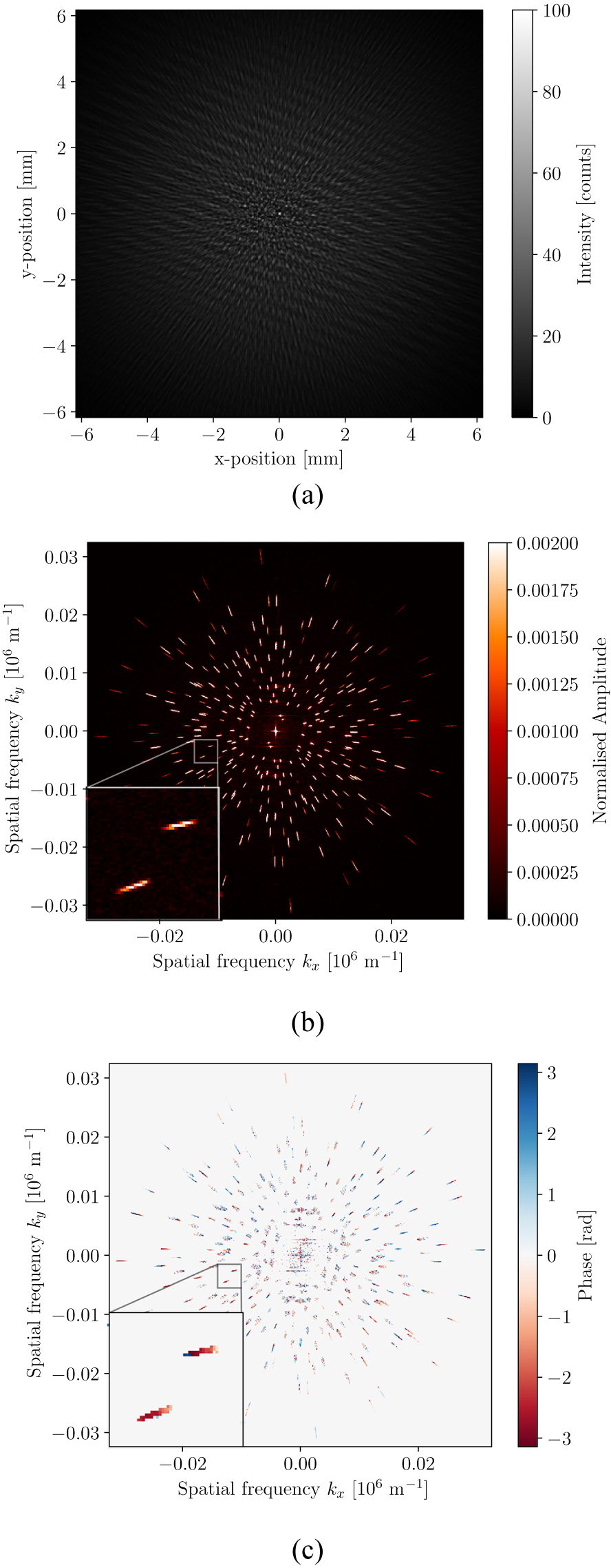
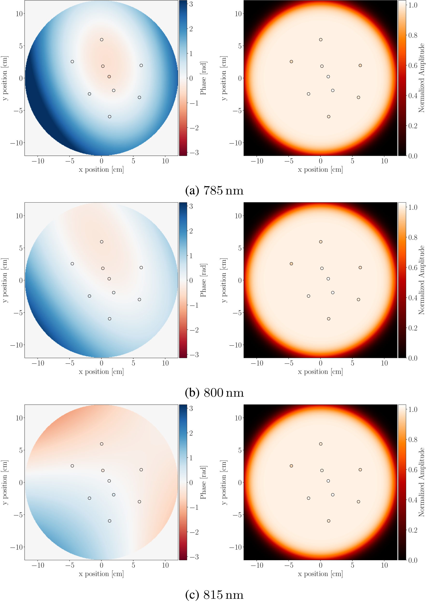
The measured far-field intensity image as well as its Fourier transform is shown in Figure 5. It can be seen that the overlying, zeroth-order Airy pattern fits well on the sensor. Also, in Figure 5(b), some, especially outer, streaks are less bright than the central ones. This indicates that the outer pinholes (for which the maximum distance to other pinholes is greater than for more central pinholes) of the mask have not been illuminated as much as the inner ones, justifying their exclusion from the reconstruction. From there, the reconstructed near-field phase and intensities are shown in Figure 6, proving the feasibility of our presented reconstruction model in this proof-of-principle. Although phase values in the reconstructed phase map seem to rise to larger values at the edge of the beam, this would probably be resolved if all pinholes were included in the reconstruction, showing a flatter phase map. Including more pinholes would also allow one to include higher-order modes in the Zernike–Taylor reconstruction[ Reference Weisse, Esslinger, Howard, Foerster, Haberstroh, Doyle, Norreys, Schreiber, Karsch and Döpp 14 ], which would allow one to fit higher-order features.
Measured intensity in the focal plane in (a) as well as the amplitude (b) and phase (c) of the Fourier-transformed image. The relative amplitudes in the Fourier domain are rather small due to the prominence of the central peak, which is the direct current (DC) offset. Although this seems to limit the resolution of amplitudes, this dominance is only in the Fourier domain due to the addition of DC peaks from each pinhole without dispersion in one spot. The actual amplitude resolution is mostly limited by the bit depth of the sensor. The phase in (c) was masked such that only physically reasonable values are shown where the amplitude is non-zero.

Figure 5 Long description
Panel a is a grayscale intensity plot. The x-axis and y-axis represent position in millimeters from minus 6 to 6. A central bright spot is surrounded by a faint, radially symmetric speckle pattern. A color bar on the right indicates intensity in counts from 0 to 100.
Panel b shows normalized amplitude in the Fourier domain. The x-axis is spatial frequency k sub x and the y-axis is spatial frequency k sub y, both in units of 10 super 6 m super minus 1, ranging from minus 0.03 to 0.03. The plot features a dense array of discrete red and orange peaks radiating from a central D C offset. An inset in the bottom-left quadrant provides a magnified view of two elongated elliptical peaks. A color bar on the right scales from 0.00000 to 0.00200.
Panel c displays the phase in radians. It uses the same spatial frequency axes as panel b. The data points correspond to the locations of the amplitude peaks in panel b but are colored according to a diverging blue-white-red scale. The color bar on the right ranges from minus 3 to 3 radians. An inset in the bottom-left shows the phase gradient within two specific peaks, transitioning from red to blue.
Reconstructed phase values (left) and relative amplitudes (right) for (a) 785 nm, (b) 800 nm and (c) 815 nm. The reconstructed phase at the pinhole position is shown as well as a full phase map from a low-order Zernike–Taylor modal reconstruction as developed in Ref. [Reference Weisse, Esslinger, Howard, Foerster, Haberstroh, Doyle, Norreys, Schreiber, Karsch and Döpp14]. The amplitude values are given relative to their mean value; the flat-top shown is visualizing this.

Figure 6 Long description
Top row, left panel: Phase map for 785 nm with x position from minus 10 to 10 centimeters and y position from minus 10 to 10 centimeters. Colorbar ranges from minus 3 to 3 radians, with blue indicating positive phase and red negative. Seven small circles mark measurement points. Top row, right panel: Normalized amplitude map for 785 nm, same axes, colorbar from 0 to 1, with a flat-top region near the center and amplitude decreasing toward the edge. Middle row, left panel: Phase map for 800 nm, similar axes and colorbar, with a different phase distribution pattern. Middle row, right panel: Normalized amplitude map for 800 nm, similar to above. Bottom row, left panel: Phase map for 815 nm, showing a distinct phase gradient. Bottom row, right panel: Normalized amplitude map for 815 nm, again with a flat-top central region. All amplitude maps show highest values at the center and lower values at the periphery. All panels have labeled axes and colorbars. The phase maps are reconstructed using low-order Zernike–Taylor modal fitting as referenced.
We estimated the uncertainty of each phase difference measurement by taking multiple images in rapid succession and estimated it to be 0.2 rad. Propagating this into the near-field phase space results in uncertainties of about 0.05 rad for each pinhole position. Further using the linear nature of the equations, we can calculate the PFT/angular dispersion to be
$0.011\pm 0.004\;\mu \mathrm{rad}\kern0.22em {\mathrm{nm}}^{-1}$
 , which is in agreement with previous measurements in this facility[
Reference Weisse, Esslinger, Howard, Foerster, Haberstroh, Doyle, Norreys, Schreiber, Karsch and Döpp
14
, Reference Howard, Esslinger, Weiße, Schröder, Eberle, Wang, Karsch, Norreys and Döpp
16
, Reference Esslinger, Weiße, Eberle, Schröder, Howard, Norreys, Karsch and Döpp
22
].
, which is in agreement with previous measurements in this facility[
Reference Weisse, Esslinger, Howard, Foerster, Haberstroh, Doyle, Norreys, Schreiber, Karsch and Döpp
14
, Reference Howard, Esslinger, Weiße, Schröder, Eberle, Wang, Karsch, Norreys and Döpp
16
, Reference Esslinger, Weiße, Eberle, Schröder, Howard, Norreys, Karsch and Döpp
22
].
5 Conclusion and outlook
In this work, we have presented a new perspective on the evaluation of the high-power laser far-field generated from a pseudo-random mask originally introduced in Ref. [Reference Smartsev, Liberman, Andriyash, Cavagna, Flacco, Giaccaglia, Kaur, Monzac, Tata, Vernier, Malka, Lopez-Martens and Faure20]. An analytical forward model enables us to determine where the crucial information, phase differences and combined intensities deduced from the initial near-field are located in the Fourier domain. This is possible as the intensity pattern in the far-field can be directly deduced from the chosen mask design. We then set up linear algebra equations to solve for the original phase values and intensities in the near-field and propagate uncertainties. We showed the option to fit a modal representation of the beam in order to deduce an approximation of the original beam. In addition, complementary methods to the experiment are presented: how to design the mask in order to obtain a viable pseudo-random pinhole pattern; how phase wrapping can be detected and corrected for by using the abundance of measurements; and how to do a final calibration of the mask position and orientation in the experiment. This not only improved the IMPALA technique but also has advantages compared to other established techniques that rely on scanning or iterative reconstruction techniques, such as TERMITES, FALCON and INSIGHT. It now allows single-shot real-time evaluation of laser pulses after the initial calibration.
We successfully tested a mask design using nine pinholes at the ATLAS-3000 laser, where the mask functioned as an attenuator as well through diffuse reflection of the majority of the beam. For the beamlets that passed the mask, no additional dispersing element influenced their properties, allowing for an unaltered reconstruction of the high-power laser pulse. This is especially significant as many diagnostics can only monitor an attenuated beam, which may differ from the original beam.
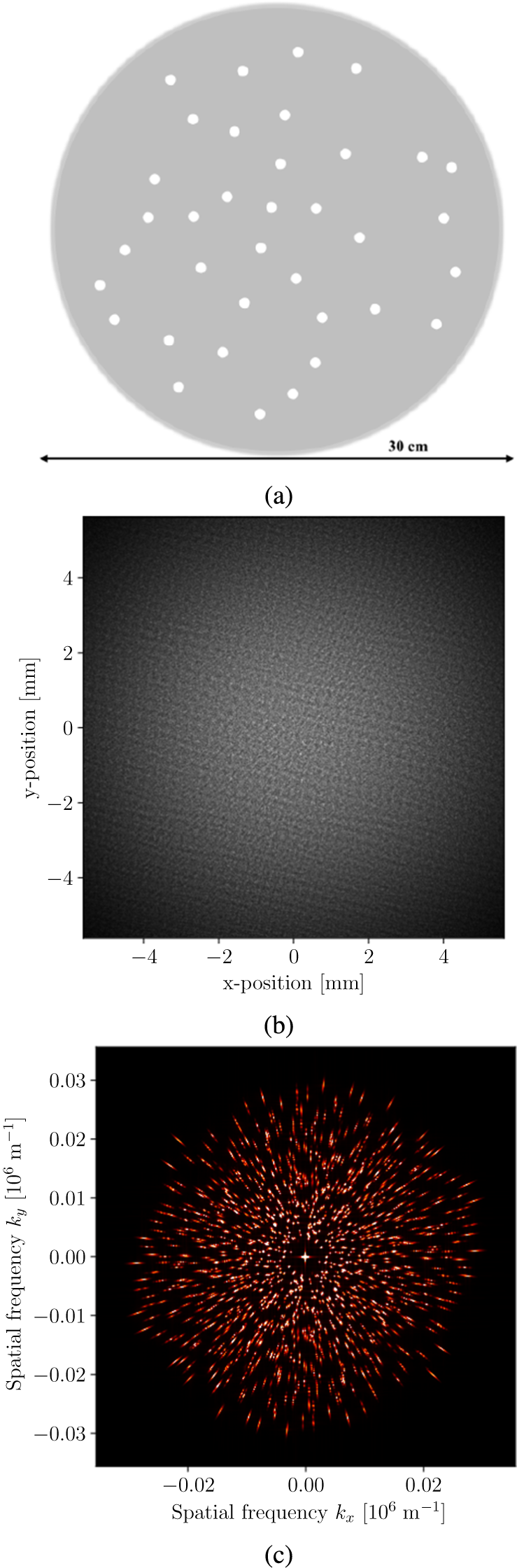
Future work may include adaptations to the general setup and mask design as well as implementing it in the daily operation routine. For the latter one may use its single-shot capabilities to monitor how the unattenuated beam profile changes over time and compare it to the other studies as shown in Refs. [Reference Howard, Esslinger, Weiße, Schröder, Eberle, Wang, Karsch, Norreys and Döpp16,Reference Esslinger, Weiße, Eberle, Schröder, Howard, Norreys, Karsch and Döpp22]. In addition, one can now compare how an attenuator alters the beam profile. In the long term, this setup can be used as a daily calibration of the attenuator in order to correct the results from complementary diagnostics that rely on an attenuated beam. Regarding an extension of the mask design, one can include more pinholes, even until the point of overloading the Fourier domain. This is shown for a potential mask designed using criteria (1)–(5) again, but with 36 pinholes, in Figure 7. Since the system is heavily overdetermined, we can rely on filtering to discard all pinhole pairs that exhibit correlation and only solve the equation system for a discrete set of frequencies and pairwise interferences. Alternatively, one can perform nonlinear retrieval, for example using alternating projections or neural networks based on the forward model, especially for matching the rate of future high-repetition-rate systems. The mask design can also be adapted to avoid outer pinholes not being illuminated properly. This can be achieved by including a safety margin in the maximum diameter of pinhole positions or by including the condition that the pinholes must lie on concentric rings to be excluded automatically if this under-illumination is detected. In addition, the experimental setup could be improved by implementing the possibility to move the mask laterally to help with the alignment.
(a) A possible mask design with 36 pinholes. The pinhole size is significantly exaggerated for visibility. (b) Simulated image in the far-field for flat phase and amplitude and a Gaussian spectrum. (c) Absolute value of the Fourier-transformed far-field intensity.

Figure 7 Long description
The figure consists of three vertically stacked panels.
Panel a is a schematic diagram of a circular gray mask. It contains 36 white dots representing pinholes arranged in a non-uniform, pseudo-random distribution. A double-headed arrow below the circle indicates a diameter of 30 cm.
Panel b is a simulated intensity plot on a dark background. The horizontal x-axis and vertical y-axis both range from minus 4 to 4 mm. The center of the plot shows a bright, diffuse Gaussian-like concentration of light that fades toward the edges, exhibiting a fine-grained speckle texture.
Panel c is a spatial frequency plot. The x-axis is labeled Spatial frequency k sub x in units of 10 super 6 m super minus 1, ranging from minus 0.02 to 0.02. The y-axis is labeled Spatial frequency k sub y in units of 10 super 6 m super minus 1, ranging from minus 0.03 to 0.03. The data appears as a dense, radial burst of red and orange points emanating from a bright central white spot. The points are distributed in a starburst pattern that fills a roughly circular area in the center of the coordinate system.
In summary, we showed a new and direct interpretation of the deterministic speckle pattern from a pseudo-random pinhole mask and used a dedicated mask for measuring a high-power laser beam without a dedicated attenuator.
Acknowledgements
We would like to thank André Kalouguine (Laboratoire d’Optique Appliquée, ENSTA Paris, CNRS, Ecole Polytechnique, Institut Polytechnique de Paris, France) for fruitful discussions, particularly regarding amplitude retrieval. This work was supported by the Independent Junior Research Group ‘Characterization and control of high-intensity laser pulses for particle acceleration’, DFG Project No. 453619281.



 Open access

