


1. Introduction
The upper ocean is a dynamically active and important region, relevant not only to Earth's climate due to exchanges at the air–sea interface, but to biogeochemical processes. Turbulence acts to vertically homogenise this upper-most layer of the ocean down to typical depths of  $10$ to $100$ m, driven by wind stresses, surface waves, heat or salinity fluxes or internal flow instabilities. Dynamics in the mixed layer influences exchanges of heat, momentum, carbon, oxygen and other important biogeochemical tracers with the ocean interior.
Fronts, or regions with large lateral density gradients, are common in the upper ocean. These lateral gradients (denoted  $\nabla_h$) of the background density field, $\bar {\rho }$ (measured by the horizontal analogue to the buoyancy frequency, $M^2\equiv g/\rho _0 |\nabla _h \bar {\rho }|$, with $g$ the acceleration due to gravity, and $\rho _0$ a reference density) are often in near-geostrophic balance and may be generated by the frontogenetic strains of mesoscale eddies, by coastal upwelling, intrusions into intermediate waters or river discharges. Additionally, persistent frontal systems in the ocean include western boundary currents (e.g. the Gulf Stream and Kuroshio) and the Antarctic Circumpolar Current.
Horizontal density gradients can drive across-front flow due to baroclinic torques,  $g/\rho _0 \nabla _h \bar {\rho } \times \hat {\boldsymbol {z}}$ (where $\hat {\boldsymbol {z}}$ is the vertical unit vector). These baroclinic torques tend to flatten isopycnals, but may be counterbalanced by a Coriolis torque, $f \partial _z \bar{\boldsymbol{u}}_{g}$ (where $f$ is the Coriolis parameter), arising from a vertical shear in the geostrophic velocity, $\bar {\boldsymbol {u}}_g$. This geostrophic balance with the horizontal gradient of hydrostatic pressure arising from the background density field is often called the thermal wind balance. The reservoir of potential energy associated with the horizontal density gradient and kinetic energy associated with the thermal wind is available to energise secondary motions. The dynamics within fronts (if not the entirety of frontal systems), however, is often unresolved in global and regional numerical models. A better understanding of these self-regulating frontal dynamics is therefore crucial to modelling the up-scale influence of unresolved processes.
Fronts are susceptible to a number of linear instabilities which drive submesoscale ( $100$ m– $10$ km) motions.
Baroclinic instability releases the potential energy stored in the horizontal density gradient, rather than extracting it from the thermal wind shear (Charney Reference Charney1947; Stone Reference Stone1972), and is a major mechanism behind the generation of submesoscale eddies (e.g. Boccaletti, Ferrari & Fox-Kemper Reference Boccaletti, Ferrari and Fox-Kemper2007; Fox-Kemper, Ferrari & Hallberg Reference Fox-Kemper, Ferrari and Hallberg2008; Callies et al. Reference Callies, Flierl, Ferrari and Fox-Kemper2016). Symmetric instability (SI) is an ageostrophic instability that can develop in frontal regions when the Ertel potential vorticity (PV)
 \begin{equation} q \equiv (\,f \hat{\boldsymbol{z}} + \boldsymbol{\nabla} \times \boldsymbol{u}) \boldsymbol{\cdot} \boldsymbol{\nabla} b, \end{equation}
(defined with the velocity,  $\boldsymbol {u}$, and buoyancy, $b\equiv -g\rho /\rho _0$) is of the opposite sign to the Coriolis parameter, $f$ (Hoskins Reference Hoskins1974). The destabilising contributions of a balanced flow are evident if we decompose the PV into a vortical and baroclinic component, respectively
 \begin{equation} q = (\omega_z + f) N^2 - M^4/f, \end{equation}
where  $\omega _z$ is the vertical component of the relative vorticity and $M^2 \equiv \partial _x \bar {b}$ (as above) is the horizontal analogue to the buoyancy frequency, $N^2 \equiv \partial _z \bar {b}$. A negative PV does not necessarily imply SI, however. In the absence of a frontal buoyancy gradient (i.e. $M^2 = 0$) ‘gravitational instability’ occurs when $N^2 < 0$ and $\omega _z + f > 0$ whereas ‘inertial instability’ occurs when $N^2 > 0$ and $\omega _z + f < 0$. Therefore SI only occurs when $(\omega _z + f) N^2 > 0$ but $M^4/f$ is sufficiently large so that $fq < 0$. Much of the ocean interior is sufficiently stratified such that $fq > 0$. However, as noted by Thomas et al. (Reference Thomas, Taylor, D'Asaro, Lee, Klymak and Shcherbina2016), a frictional stress or diabatic flux at the surface and bottom boundaries lead to $fq < 0$ and trigger SI.
In the context of the Eady model with uniform horizontal and vertical buoyancy gradients, Stone (Reference Stone1966) found that symmetric modes, defined as those independent of the along-front direction (i.e. perpendicular to the horizontal buoyancy gradient), grow faster than baroclinic modes (independent of the cross-front direction) for  $Ri < 0.95$, where $Ri\equiv N^2f^2/M^4$ is the balanced Richardson number. Stone (Reference Stone1971) considered the non-hydrostatic contributions to symmetric and baroclinic instabilities in the ageostrophic Eady model, showing that the vertical inertia suppresses both baroclinic and symmetric instabilities. Viscous contributions to the bounded non-hydrostatic SI problem were then included by Weber (Reference Weber1980) and approximated by a viscosity acting on a vertically unbounded normal mode. Beyond the Eady model other types of instability are possible. For example, Wang, McWilliams & Ménesguen (Reference Wang, McWilliams and Ménesguen2014) describe a variety of instabilities that develop in more general vertically sheared flows and how they relate to symmetric and baroclinic instability in the Eady model.
Recent observational studies have accumulated evidence of SI in the ocean. For example, increased turbulence and dissipation (exceeding that from atmospheric forcing) in regions where  $fq < 0$ has been attributed to SI (Thomas et al. (Reference Thomas, Taylor, D'Asaro, Lee, Klymak and Shcherbina2016) in the Gulf Stream, and D'Asaro et al. (Reference D'Asaro, Lee, Rainville, Harcourt and Thomas2011) in the Kuroshio). This negative PV is generated by atmospheric forcing – either by upward buoyancy fluxes (for example cooling) (Haine & Marshall Reference Haine and Marshall1998; Thomas et al. Reference Thomas, Taylor, Ferrari and Joyce2013) or wind stresses (Thomas & Lee Reference Thomas and Lee2005) – which can reduce the PV, and sustain ‘SI turbulence’ and mixing stronger than what the forcing alone could generate. Thompson et al. (Reference Thompson, Lazar, Buckingham, Naveira Garabato, Damerell and Heywood2016b) and later Yu et al. (Reference Yu, Naveira Garabato, Martin, Gwyn Evans and Su2019) have also found evidence for SI in glider and mooring observations of the open ocean away from major frontal systems. Recently, Savelyev et al. (Reference Savelyev2018) captured aerial images of SI in the North Wall of the Gulf Stream (cf. figure 2), which constitutes the only visual evidence of the structure of SI to date.
Vertically sheared inertial oscillations of the isopycnals can result from the rapid mixing of geostrophic momentum, and were present following the saturation of SI in the simulations of Taylor & Ferrari (Reference Taylor and Ferrari2009). Tandon & Garrett (Reference Tandon and Garrett1994) modelled the response of a mixed layer front to impulsive vertical mixing using the inviscid hydrostatic equations. After a mixing event, the front undergoes inertial oscillations and modulates the background stratification about the average steady-state position ( $Ri = 1$). Tandon & Garrett (Reference Tandon and Garrett1994) also considered the case when the vertical stratification is perfectly homogenised (for example by a passing storm), but where the geostrophic shear is partially mixed leaving only a fraction, $s$, of the balanced shear profile. We will show that when acting on times short relative to the inertial period, then SI can generate sufficient geostrophic momentum transport needed to prompt adjustment. We quantify this mixing fraction, $(1-s)$, resulting from the effects of SI.
A number of previous numerical process studies of SI have investigated its nonlinear evolution with varying set-ups, but most have focused only on a single value of the non-dimensional horizontal buoyancy gradient (Thomas & Lee Reference Thomas and Lee2005; Taylor & Ferrari Reference Taylor and Ferrari2009, Reference Taylor and Ferrari2010; Thomas & Taylor Reference Thomas and Taylor2010; Stamper & Taylor Reference Stamper and Taylor2016). Nonetheless, between persistent fronts, transient fronts and mid-ocean fronts, the strength of these horizontal buoyancy gradients span a large range in the ocean (Hoskins & Bretherton Reference Hoskins and Bretherton1972; Jinadasa et al. Reference Jinadasa, Lozovatsky, Planella-Morató, Nash, MacKinnon, Lucas, Wijesekera and Fernando2016; Thompson et al. Reference Thompson, Lazar, Buckingham, Garabato, Damerell and Heywood2016a). We therefore vary the front strength,  $\varGamma \equiv M^2/f^2$, rather than changing the vertical stratification as measured by $Ri$.
$Ri$.
In this paper, we investigate the equilibration of SI-unstable fronts. We focus on the development and saturation of SI in the Eady model configuration to determine the transport by SI and explain how the rate of energy extraction and amplitude of the resulting inertial oscillations vary with frontal strength. To do this, we first extend the non-hydrostatic and bounded linear analysis of Stone (Reference Stone1971) to include viscosity. We represent the vertical viscous terms using the wave-mode approximation of Weber (Reference Weber1980) to find an analytic solution, but further solve the full numerical eigensystem to verify this approximation in the regime of interest. Compared with Stone (Reference Stone1966) and ensuing papers which studied instability of the Eady model in the inviscid, hydrostatic limit, our analysis is no longer a function only of  $Ri$, but now also depends on the front strength, $\varGamma$.
These purely linear analyses are unable to determine the finite contribution of SI to the momentum transport, buoyancy fluxes and energetics of the flow. We analyse the weakly nonlinear problem by considering the growth of secondary instabilities on the growing finite-amplitude SI modes. Our analysis formally extends the work by Taylor & Ferrari (Reference Taylor and Ferrari2009) who implicitly considered the secondary shear instability of (unbounded) SI modes by applying the Miles–Howard theorem. We are thereby able to compute a critical amplitude beyond which SI transitions to turbulence and calculate the efficiency with which SI mixes geostrophic momentum prior to transition. To our knowledge this is the first calculation of the mixing fraction,  $(1-s)$, (as used by Tandon & Garrett (Reference Tandon and Garrett1994) to describe the geostrophic response of a front) associated with SI.
We begin in § 2 by introducing the problem set-up and primary linear stability analysis for SI. In § 2.3, we consider the stability of these growing SI modes to secondary shear instability and find a critical mode amplitude beyond which the front transitions to turbulence. We finally combine these two stability analyses in §§ 4 and 5 to determine the finite-amplitude contributions of SI to the energetics and momentum transport, respectively.
In a companion paper, we explore the nonlinear consequences of these findings beyond the saturation point. We extend the numerical simulations (from § 3 here used for validation) to study the evolution of these fronts following SI. We use the framework of Tandon & Garrett (Reference Tandon and Garrett1994) to shed light on the effects of dissipation and a finite mixing time on the adjustment response and resulting inertial oscillations.
2. Linear stability analysis
Perhaps the simplest model of a front, the Eady model was first introduced by Eady (Reference Eady1949) and later used by Stone (Reference Stone1966, Reference Stone1970) to study ageostrophic instabilities. As illustrated in figure 1, the Eady model can be viewed as a local idealisation of a submesoscale mixed layer front where the bottom of the mixed layer is replaced with a flat, rigid boundary. Specifically, an incompressible flow in thermal wind balance with uniform horizontal and vertical buoyancy gradients is bounded between two rigid, stress-free horizontal surfaces.
Schematic of a model frontal region showing coloured contours of density varying both across the front and vertically. The across-front stratification is balanced by the thermal wind shear in  $\bar {v}_g$, shown on the top face. A local horizontally homogeneous model can be constructed by considering the region within the grey box, where the buoyancy gradient is approximately uniform.

Non-dimensionalising the Eady problem such that the thermal wind shear,  $M^2/f$, is unity in units where the vertical domain size, $H = 1$, brings out four dimensionless parameters
 \begin{equation} \varGamma \equiv \frac{M^2}{f^2}; \quad Re \equiv \frac{H^2 M^2}{f \nu}; \quad Ri \equiv \frac{N^2 f^2}{M^4}; \quad Pr \equiv \frac{\nu}{\kappa}.\end{equation}
Here,  $\nu$ is the kinematic viscosity and $\kappa$ is the diffusivity of buoyancy, but we take $Pr = 1$. It should be noted that the Rossby number is not a parameter in this local frontal zone configuration because there is no horizontal length scale.
We consider a range of front strengths,  $\varGamma =M^2/f^2 \approx [1,100]$, which covers a wide variety of ocean fronts. Although very strong fronts with $\varGamma >100$ have been observed (e.g. Sarkar et al. Reference Sarkar, Pham, Ramachandran, Nash, Tandon, Buckley, Lotliker and Omand2016), these fronts are typically very narrow and hence our assumption of a uniform horizontal density gradient is expected to break down. The development of SI at very strong ( $\varGamma >100$) and narrow fronts will be reserved for future work.
2.1. Governing equations
Here, we invoke the Boussinesq approximation with a linear equation of state. We further assume that the Coriolis parameter,  $f$, is constant and neglect the non-traditional Coriolis terms (i.e. those proportional to $\tilde {f} = 2\varOmega \cos \phi$, where $\varOmega$ is the angular velocity and $\phi$ is latitude). This ‘traditional’ approximation is made here for simplicity but is shown in Appendix A to not qualitatively change our conclusions. The resulting non-dimensionalised Boussinesq equations are
 $$\begin{gather} \frac{\textrm{D} \boldsymbol{u}^*}{\textrm{D} t^*} ={-}\boldsymbol{\nabla}^*\varPi^* - \frac{1}{\varGamma} \hat{\boldsymbol{z}}\times \boldsymbol{u}^* + \frac{1}{Re} \nabla^{*2}\boldsymbol{u}^* + b^* \hat{\boldsymbol{z}}, \end{gather}$$
 $$\begin{gather}\frac{\textrm{D} b^*}{\textrm{D} t^*} = \frac{1}{Re} \nabla^{*2} b^*, \end{gather}$$
 $$\begin{gather}0 = \boldsymbol{\nabla}^*\boldsymbol{\cdot} \boldsymbol{u}^*. \end{gather}$$
Consistent with the non-dimensional parameters (2.1a–d) introduced above, the dimensionless ( $^*$) variables here are
 \begin{equation} \boldsymbol{u}^* \equiv \boldsymbol{u}\frac{f}{H M^2}; \quad b^* \equiv b \frac{f^2}{H M^4}; \quad t^* \equiv t \frac{M^2}{f}; \quad \boldsymbol{x}^* \equiv \boldsymbol{x}\frac{1}{H}; \quad \boldsymbol{\nabla}^* \equiv H \boldsymbol{\nabla}. \end{equation}
The dimensionless pressure head acceleration,  $\boldsymbol{\nabla}^* \varPi ^*$, absorbs the hydrostatic pressure gradient, and is eliminated when writing (2.2a) with the along-front streamfunction.
We choose  $\hat {\boldsymbol {x}}$ to be the across-front direction (parallel to $\nabla _h \bar {b}$). The background basic state (denoted by an overbar) used for linearisation and the initial condition for the numerical simulations is
 \begin{equation} \left. \begin{array}{c@{}} \bar{v}^* = z^* - 1/2 \\ \bar{b}^* = \varGamma^{{-}1} x^* + Ri z^* \end{array} \right\}, \end{equation}
as shown in the grey shaded region of figure 1. Following the Eady model, we will also use solid horizontal boundaries at  $z^* = 0$ and $1$ which are taken to be insulating and stress free (Eady Reference Eady1949). In what follows we will omit the appended asterisks for notational simplicity. All variables are dimensionless unless the units are explicitly stated (as in some figures).
2.2. Primary instability
We begin by linearising the Boussinesq equations (2.2) about the basic state (2.4) to describe the evolution of small anomalies in buoyancy and momentum, denoted with a prime. Since the most unstable mode of SI is independent of the along-front ( $\hat {\boldsymbol {y}}$) direction (Stone Reference Stone1966), we consider linear perturbations that vary only in $x$ and $z$:
$z$:
 \begin{equation} \left. \begin{array}{c@{}} \displaystyle \partial_t u' ={-}\partial_x \varPi' + \dfrac{1}{\varGamma} v' + \dfrac{1}{Re}\nabla^2 u' \\ \displaystyle \partial_t v' + w'\partial_z\bar{v} ={-}\dfrac{1}{\varGamma} u' + \dfrac{1}{Re}\nabla^2 v' \\ \displaystyle \partial_t w' ={-}\partial_z \varPi' + \dfrac{1}{Re}\nabla^2 w' + b'\\ \displaystyle \partial_t b' + u'\partial_x\bar{b} + w'\partial_z\bar{b} = \dfrac{1}{Re}\nabla^2 b'\\ 0 = \boldsymbol{\nabla}\boldsymbol{\cdot} \boldsymbol{u}' \end{array}\right\}. \end{equation}
We transform this set of partial differential equations (PDEs) into a set of ordinary differential equations (ODEs) by further assuming normal mode perturbations autonomous in  $x$ (with wavenumber $k_x$) and in time (with frequency $\omega$) of the form
 \begin{equation} \chi'(x,z,t) = \Re [ \hat{\chi}(z) \, \mathrm{e}^{\mathrm{i}(k_x x - \omega t)} ], \end{equation}
where the eigenfunction,  $\hat {\chi }(z)$, must then be chosen to satisfy the relevant boundary conditions. The set (2.5), after substitution and simplification using the streamfunction defined by $(u',w') = \boldsymbol {\nabla }\times \psi \hat {\boldsymbol {y}}$, becomes
 \begin{equation} \left(\mathrm{i}\omega + \frac{1}{Re}({-}k_x^2 + D^2)\right)^2({-}k_x^2+D^2)\hat{\psi} = \left(-\frac{1}{\varGamma^2}D^2 -\frac{2\mathrm{i}k_x}{\varGamma}D + k_x^2 Ri\right) \hat{\psi}, \end{equation}
where  $D \equiv \mathrm {d}/\mathrm {d}z$ for notational ease. Note that this equation is closely related to (14) in Grisouard & Thomas (Reference Grisouard and Thomas2016) who formulated the equation in terms of pressure and neglected horizontal diffusion. The boundary conditions for $\hat {\psi }$ at $z = 0, 1$ on this sixth-order ODE are
 \begin{equation} \left. \begin{array}{c@{}} \hat{\psi} = 0\\ D^2 \hat{\psi} = 0 \end{array} \right\}. \end{equation}
To make this system tractable, we follow the method of Weber (Reference Weber1980) and approximate equation (2.7) as a second-order ODE by writing the vertical diffusion terms as spatially invariant wave modes,
 \begin{equation} \frac{1}{Re} D^2 \hat{\psi} \approx{-}\frac{1}{Re} k_z^2 \hat{\psi}, \end{equation}
with vertical wavenumber  $k_z$. By neglecting the vertical variations in $k_z$, this approximation constrains the SI mode angle to be uniform in $z$. This is a good approximation for large $Re$ and $k_z$, when the effects of diffusion are dominated by the interior of the domain. This does consequently prohibit the boundaries from generating vorticity, but it is found to not influence the selection or stability of SI, which is only energised by the bulk background buoyancy and shear. Equation (2.7) then becomes
 \begin{align} \left[\left(\mathrm{i}\omega -
\frac{k_x^2 + k_z^2}{Re}\right)^2 + \frac{1}{\varGamma^2}\right]
D^2\hat{\psi} + \frac{2\mathrm{i}k_x}{\varGamma}
D\hat{\psi} -k_x^2\left[\left(\mathrm{i}\omega -
\frac{k_x^2+k_z^2}{Re}\right)^2 + Ri\right] \hat{\psi} =
0,\end{align}
\begin{align} \left[\left(\mathrm{i}\omega -
\frac{k_x^2 + k_z^2}{Re}\right)^2 + \frac{1}{\varGamma^2}\right]
D^2\hat{\psi} + \frac{2\mathrm{i}k_x}{\varGamma}
D\hat{\psi} -k_x^2\left[\left(\mathrm{i}\omega -
\frac{k_x^2+k_z^2}{Re}\right)^2 + Ri\right] \hat{\psi} =
0,\end{align}which has eigensolutions of the form
 \begin{equation} \hat{\psi} = \exp(\mathrm{i} \lambda_1 z) - \exp(\mathrm{i} \lambda_2 z),\end{equation}
that match the boundaries if  $\lambda _1 - \lambda _2 = 2{\rm \pi} n$, for the chosen eigenmode number, $n$. Equation (2.10) is thus reduced to a quadratic eigenproblem which may be solved by numerical iteration while enforcing the vertical viscous wave-mode approximation that
 \begin{equation} k_z^2 = \tfrac{1}{2} (\lambda_1^2 + \lambda_2^2). \end{equation}
Complete details of this solution are included in Appendix B.1.
The exact numerical eigensolution to the linear set (2.5) was also computed using a pseudo-spectral eigenvalue solver written in Matlab. The computed solutions to (2.10) give good agreement with this numerical solution, as shown in figure 2(a), where the growth rate,  $\sigma$, is the imaginary part of $\omega$. This new solution correctly accounts for both the limiting effects of the vertical boundaries at low wavenumber, and of viscosity at high wavenumber. Accurate in the low wavenumber limit, Stone (Reference Stone1971) determined this inviscid, bounded solution, where the mode growth becomes suppressed as it feels the constraint of the boundaries for $k_x \lesssim 2{\rm \pi}$. In the other limit of unbounded, viscous and hydrostatic motions, Taylor & Ferrari (Reference Taylor and Ferrari2009) (and later Bachman & Taylor (Reference Bachman and Taylor2014) for non-hydrostatic motions) found that the most unstable mode has a vanishing wavenumber. The structure of the exact ( $n = 1$) viscous, bounded SI mode ( $u'$) is shown in the background of figure 4. Due to viscous and non-hydrostatic effects, the modes are no longer parallel to isopycnals as they were in e.g. Stone (Reference Stone1966).
(a) The growth rate for the  $n=1$ SI mode in a vertical front with $\varGamma = 10$ and $Re = 10^5$. The real part of $\omega$ for the SI modes are everywhere $0$ except where linearly stable at very small wavenumber. (b) The growth rate of the fastest growing SI mode ( $n=1$) and wavenumber at $Re = 10^5$, as a function of $\varGamma$. The vertical front ( $Ri = 0$) is shown in black and also for increasing stratification.

We can now consider how the fastest growing mode of (2.10) varies with  $\varGamma$ and $Ri$, as shown in figure 2(b). For $Ri=0$ the energy growth rate relative to $f$ increases nearly linearly with front strength. However, for strong fronts stratification significantly reduces the growth rate of the most unstable modes.
In a vertically unbounded domain with an inviscid, hydrostatic dynamics, the maximum release of energy can be achieved by motion aligned with  $b$ surfaces, with ${\theta _b = \tan ^{-1}(M^2/N^2)}$ from the horizontal (i.e. $k_x/k_z = M^2/N^2$) (Taylor & Ferrari Reference Taylor and Ferrari2009), effectively precluding any buoyancy flux. However, in a vertically bounded front with weak stratification, the most unstable modes become very inclined to the isopycnals as shown in figure 3(a), and reach nearly $45^\circ$ for $N^2 = 0$. While the angle of the unstable SI modes must still be between the angle of the isopycnals and surfaces of constant absolute momentum ( $\bar {m} = \bar {v}_g + \varGamma ^{-1} x$) (dotted and dash-dotted curves in figure 3a), the most unstable modes approach more closely to the angle of the absolute momentum surfaces ( $\theta _m = \tan ^{-1}\varGamma ^{-1}$) for small front strength. This permits a larger buoyancy production of energy ( $\mathcal {B} = \langle w'b' \rangle$), as shown in figure 3(b), while the geostrophic shear production ( $\mathcal {P}_g = -\langle \overline {v'w'} \partial _z \bar {v}_g \rangle$) is the dominant energy source in the rest of the parameter space. Here and throughout the rest of this paper, $\langle \cdot \rangle$ indicates a volume average over the entire domain, and primes represent local departures from the horizontally averaged fields denoted by $\bar {\cdot }$.
(a) The angle of the fastest growing SI mode as measured from horizontal, plotted as a function of front strength,  $\varGamma$, and for different background stratifications measured by the inverse isopycnal slope, $N^2/M^2$. The shaded grey region indicates where $fq>0$ and the front is stable to SI. The unstable SI mode inclination must remain between the angle of absolute momentum surfaces ( $\theta _m$, dot-dashed line) and isopycnals ( $\theta _b$, dotted lines), which for $N^2/M^2 = 0$, $\theta _b = 90^\circ$. This unstratified case has modes nearly equally spaced between the isopycnals and absolute momentum surfaces for large $\varGamma$, but with increasingly horizontal isopycnals the SI modes grow more along these isopycnals. While the angle of the contour $\psi (x,z)=0$ is a weak function of $z$ in the full numerical eigensolution (decreasing by at most $5\,\%$ at the boundaries), the mode angle of the solutions (2.11) are independent of $z$. (See Appendix B.1 for details on the calculation of $\theta$ and the eigenfunctions.) (b) Contribution of the most unstable linear SI mode to the energy budget (4.1) of the vertical front for $Re = 10^5$. Normalised by the kinetic energy, the geostrophic shear production and buoyancy flux are relatable to the growth rate, $\sigma$. As expected with SI, the instability still primarily draws energy from the thermal wind shear into the kinetic energy of the mode through the TKE production term. The grey dotted line indicates the growth rate of baroclinic instability for this choice of parameters (Stone Reference Stone1966). Symbols correspond to the numerical simulations discussed in § 3, computed as a time average from $t=0$ to $\tau _c/2$.

2.3. Secondary instability
Secondary instability plays a key role in the equilibration of SI. Here, we explore the onset of secondary instability to determine the cumulative effects of SI in the front equilibration energetics and the contribution to mixing down the thermal wind shear.
As described in Taylor & Ferrari (Reference Taylor and Ferrari2009), shear associated with the growing SI modes becomes unstable to a secondary Kelvin–Helmholtz instability (KHI) which prompts a transition to turbulence. We identify this critical SI mode amplitude,  $U_{SI} = U_c$, at which the SI modes themselves break down as the time when the SI growth rate, $\sigma _{SI}$, is equal to the KHI growth rate, $\sigma _{KH}$. Of course, $\sigma _{KH}$ is a monotonically increasing function of the shear, and thereby of $U_{SI}$ which exponentially grows at a rate $\sigma _{SI}$. We therefore iteratively compute the secondary linear stability of the combined Eady and growing SI mode basic state to determine this critical amplitude that is plotted in figure 5(a).
We formulate the one-dimensional (1-D) linear Kelvin–Helmholtz stability problem using a sinusoidal extension of the structure of the full SI mode (evaluated at the mid-plane) in the rotated coordinates shown in figure 4. As described in Appendix C, this basic state includes the constant vertical and horizontal buoyancy gradients associated with the basic state in the Eady model as well as the buoyancy changes induced by the SI modes. We iteratively compute  $\sigma _{KH,max}(U_{SI})$ with a pseudo-spectral solver until finding the critical SI mode amplitude, $U_{c}$. While the most unstable SI wavevector, $|\boldsymbol {k}_{SI}|$, increases as the mode number ( $n$) and $Re$ increase, the scaling for $U_{c}$ appears to be dominated by $\sigma _{SI}$ and so remains largely unchanged.
Diagram showing the secondary stability analysis coordinate transformation drawn over the linear SI mode ( $u'$). The primary SI basic state is also indicated, with grey isopycnal lines showing the linearly increasing buoyancy from left to right (for $Ri = 0$), as well as the thermal wind vectors into the page which balance the baroclinic torques.

We demonstrate this here just for the unstratified ( $Ri = 0$) front, but a general analysis is provided in Appendix C. Figure 5(a) shows the classic KH stability analysis (i.e. ignoring rotation and neglecting the along-mode component of the background stratification) alongside the full solution for $U_{c}$. The dashed line shows the resulting scaling,
 \begin{equation} U_{c} \propto (\sqrt{\varGamma} |\boldsymbol{k}_{SI}|)^{{-}1}, \end{equation}
(in our same dimensionless units of the velocity associated with thermal wind shear). We obtain this scaling by balancing the KHI growth rate (proportional to the non-dimensional shear in the SI mode,  $\sigma _{KH}\propto U_{c} |\boldsymbol {k}_{SI}|$) with the SI growth rate in the limit of large $\varGamma$, $\sigma _{SI} \propto \varGamma ^{-1/2}$. We see that this simple scaling argument fails for small $\varGamma$ where the growth rate in these weak fronts is slow compared with $f$.
$f$.
(a) The critical amplitude of the most unstable SI mode velocity at which secondary instability begins to dominate, shown in units of the thermal wind. The dotted line shows this critical amplitude when rotation and along-shear stratification (i.e.  $x^{\dagger}$ in Appendix C) are neglected in the KHI stability analysis. The dashed line shows the scaling (2.13) achieved by taking the KHI growth rate directly proportional to the shear and matching $U_c$ in the limit of large $\varGamma$. (b) The cumulative kinetic energy (KE) budget contributions from the $n = 1$ linear SI mode of the unstratified front, integrated through $U_{c}$. Coloured symbols show the value derived from the 2-D simulations. Due to weak scale and mode selection, these simulations contain a range of $n$ and $k_x$, yet with increasing front strength the values calculated from the simulations approach the $n = 1$ line shown due to stronger mode selection as the higher modes are damped by viscosity.

3. Numerical simulations
We employed the non-hydrostatic hydrodynamics code, diablo, to verify the conclusions of the preceding linear primary and secondary instability theory as well as the results in the following two sections. diablo solves the fully nonlinear Boussinesq equations (2.2) on an  $f$-plane (Taylor Reference Taylor2008). Second-order finite differences in the vertical and a collocated pseudo-spectral method in the horizontal periodic directions are employed, along with a third-order accurate implicit–explicit time-stepping algorithm using Crank–Nicolson and Runge–Kutta with an adaptive step size. Rigid, stress-free and insulating horizontal boundaries are enforced to match the linear analysis in § 2. Following Taylor & Ferrari (Reference Taylor and Ferrari2009), the simulations are run in a 2-D ( $x$–
$x$– $z$) domain while retaining all three components of the velocity vector. This choice allows us to focus on the evolution and saturation of the symmetric modes.
While the presented analytical results in this paper are general, we focus these numerical verification experiments on an initially unstratified front ( $Ri=0$) with ${Re = 10^5}$. It should be noted that the along-front flow would be susceptible to KHI in a 3-D simulation, but this is not considered for the purpose of this study. Each of the simulations were initialised as a balanced front (2.4) with strength ${\varGamma = \{1, 10, 100\}}$ and white noise was added to the velocity with a (dimensionless) amplitude of $10^{-4}$. The simulations were run through the linear phase until secondary instability breaks down the SI modes at the critical time, $\tau _c$, as shown in the right column of figure 6. At this point, we measure the cumulative effects of SI on the front – the integrated shear production, buoyancy fluxes and momentum transport – and present these values alongside the analytical results of §§ 4 and 5. While we restrict these verification simulations to initially unstratified fronts and do not consider times after $\tau _c$, we extend these simulations in a companion paper to explore the SI-induced re-stratification and geostrophic adjustment of the fronts at later times.
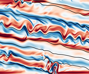
Slices across each front show the along-front vorticity,  $\omega _y$, along with buoyancy contours (black lines), for $\varGamma = 1$ (top), $10$ (centre) and $100$ (bottom). Two snapshots are shown, at $t = \tau _c/2$ (left) when the fastest linear SI mode has emerged, and at $t = \tau _c$ (right) when secondary KHI first begins to break the coherent energy of the SI modes into small-scale turbulence. Note that the vorticity is normalised by $M$, which keeps the amplitude similar across the range of $\varGamma$ (consistent with the scaling (2.13)). The vorticity normalised by $f$ can be obtained by multiplying the values shown here by $\varGamma ^{-1/2}$. During the linear growth phase (left panels), the SI modes do not align with the isopycnals, and rather become increasingly flat for larger $\varGamma$, consistent with the results shown in figure 3(a).

4. Energetics of SI
In light of these stability analyses, a natural question is: What impact does the linear SI phase and ensuing turbulence have on the resulting equilibration of the front, and how does it depend on the frontal strength? To answer this, we combine the primary linear instability results of § 2.2 with the details of SI saturation from § 2.3 to determine the cumulative contribution of SI modes up to the critical time,  ${\tau _c = \sigma _{SI}^{-1}\log (U_c/U_0)}$, when SI has grown to an amplitude $U_{c}$. This allows us to quantify the energetics of the linear SI modes and their influence on the evolution of the front.
With the complex eigenfunction,  $\hat {\psi }$, found by iteratively solving for $\lambda _1$ and $\lambda _2$ in (2.11), we determined the full structure of these modes: $\hat {u}$, $\hat {v}$, $\hat {w}$ and $\hat {b}$ as given in Appendix B.1. With these, we compute the correlations relevant to the transport and energetics of the development of SI. We first must normalise each of the modes by $\sqrt {|\hat {u}|^2 + |\hat {w}|^2}$, and then rewrite them in the normal mode form, (2.6), using the parameter and eigenvalues of (2.10).
We will first consider the contribution of SI to the turbulent kinetic energy (TKE),  ${E_K \equiv \frac {1}{2} \langle u_i' u_i'\rangle }$:
 \begin{equation} \frac{\partial E_K}{\partial t} ={-}\underbrace{\left\langle \overline{u'w'}\frac{\partial\bar{u}}{\partial z}\right\rangle }_{-\mathcal{P}_x} - \underbrace{\left\langle \overline{v'w'}\left(\frac{\partial\bar{v}_a}{\partial z} + \frac{\partial\bar{v}_g}{\partial z}\right)\right\rangle }_{-\mathcal{P}_y} + \underbrace{\left\langle w'b'\right\rangle }_\mathcal{B} - \underbrace{\frac{1}{Re}\left\langle \frac{\partial u'_i}{\partial x_j}\frac{\partial u'_i}{\partial x_j}\right\rangle }_{\varepsilon_t}. \end{equation}
The first two terms on the right-hand side represent the shear production,  $\mathcal {P}$, converting energy from the mean flow into TKE. Specifically, the along-front contribution ( $\mathcal {P}_y$) is split into a geostrophic shear production term, $\mathcal {P}_g$, energised by the thermal wind shear, and an ageostrophic part. The other potential source of TKE comes from buoyancy production, $\mathcal {B}$, which represents the transfer of energy from PE into TKE. The cumulative generation of TKE by each of these terms in (4.1), integrated from $t = 0$ up to transition at $\tau _c$ is shown in figure 5(b). As expected for SI, the contribution from $\mathcal {P}_g$ exceeds $\mathcal {B}$, except for small $\varGamma$. Interestingly, even for these SI modes that are very flat (i.e. inclined to the isopycnals) in strong fronts, the energetics are still dominated by geostrophic shear production which relies on the vertical velocity to exchange geostrophic momentum. We confirm this result using the numerical simulations described in § 3. Even though the initial white noise and weak mode selection mean that a range of wavenumbers are represented in the simulations, these predictions still remain robust.
Following Haine & Marshall (Reference Haine and Marshall1998), it is possible to re-frame the SI stability criterion,  $fq < 0$, in terms of the energy sources driving growth: the background buoyancy gradient and the geostrophic kinetic energy. First consider fluid parcels that are constrained to move along isopycnals (and thus incur no gravitational penalty). The criterion, $fq < 0$, for instability then becomes the Rayleigh criterion describing inertial instability,
 \begin{align}
f\left(\frac{\partial m}{\partial x}\right)_b < 0.\end{align}
\begin{align}
f\left(\frac{\partial m}{\partial x}\right)_b < 0.\end{align}
where the subscript here indicates the gradient is measured along isopycnals. Since they are aligned with the isopycnals, these modes do not extract potential energy from the front and instead grow by drawing energy from the thermal wind. Contrast this with the other limiting angle that SI modes can take, when their motion is aligned with surfaces of constant absolute momentum. Now, instability requires that the vertical buoyancy gradient measured along these absolute momentum surfaces is negative
 \begin{equation} \left(\frac{\partial b}{\partial z}\right)_m < 0. \end{equation}
Therefore, motions that are constrained to follow absolute momentum surfaces can extract potential energy, analogously to ‘upright convection’ (Haine & Marshall Reference Haine and Marshall1998). For hydrostatic perturbations in an unbounded domain, the most unstable mode of SI is aligned with the isopycnals and hence grows by extracting kinetic energy from the thermal wind through geostrophic shear production (Stone Reference Stone1972; Haine & Marshall Reference Haine and Marshall1998; Taylor & Ferrari Reference Taylor and Ferrari2009).
As shown previously in figure 3(a), for non-hydrostatic modes in a bounded domain, the most unstable mode of SI is not necessarily aligned with isopycnals and hence these modes can grow through a non-trivial combination of buoyancy production and geostrophic shear production. We can quantify the energetic influences on the most unstable mode of SI using the linear stability analysis up to the critical time,  $\tau _c$. We do this by introducing the energy production ratio,
 \begin{equation} \frac{\mathcal{B}}{\mathcal{B}+\mathcal{P}_g} = \frac{\lambda_1 + \lambda_2}{2 k_x \varGamma}, \end{equation}
as plotted in figure 7, where  $\mathcal {B}$ is the buoyancy flux, $\mathcal {P}_g$ is the geostrophic shear production and $\lambda _1$ and $\lambda _2$ describe the vertical mode structure (2.11) and depend on $Ri$ and $\varGamma$ (details of which are given in Appendix B.2). The production ratio suggests the expected character of SI. For strong fronts with weak vertical stratification, SI extracts energy from shear production, and so we refer to this flavour of SI as ‘slantwise inertial instability’. In the inviscid and hydrostatic limits, the linear analysis indicates that energy is always fully derived from geostrophic shear production, with modes aligned perfectly with isopycnals at $\theta _b$. Non-hydrostatic effects flatten the SI modes particularly for small $\varGamma$. This permits buoyancy production to contribute to the energy more than shear production, and so we call this flavour of SI ‘slantwise convection’. Note that this term has sometimes been used synonymously with SI in the literature, although it is not always congruous with the energetics of SI (Haine & Marshall Reference Haine and Marshall1998). The boundary-permitted viscous limit in figure 7(b) each for large $\varGamma$ and large $Ri$ also exhibits slantwise convection modes. It is perhaps then surprising that within the white outlined region, indicating where SI modes are more aligned with isopycnals, the instability does not always extract a majority of energy from the shear production (i.e. red shading).
Contours of the production ratio (4.4) distinguish regions where geostrophic shear production dominates ( $0$) and regions where buoyancy production dominates ( $1$). The white line separates regions of parameter space where SI modes are more aligned with isopycnals, i.e. $|\theta -\theta _b|< |\theta -\theta _m|$ (inside), from the regions (outside) where they are more closely aligned with absolute momentum surfaces. (a) The production ratio plotted in parameter space with $N^2/f^2$ on the $y$-axis, chosen so that the axes are only interdependent on $f$. A black dashed line designates the contour $Ri = 0.25$. Lines of constant isopycnal slope ( $M^2/N^2$) are straight lines of slope $1$ in this log–log scale. Strong fronts with weak stratification (equivalently, large isopycnal slope) derive energy primarily from geostrophic shear production. Thus, rapid frontogenesis (moving horizontally to the right), or rapid de-stratification via mixing (moving vertically downwards) will tend the SI modes to slantwise inertial instability. (b) The parameter space is rescaled with $Ri$ on the $y$-axis to emphasise the region near $Ri = 1$ where SI in a balanced front becomes stabilised. Non-hydrostatic effects (for small $\varGamma$) and boundary viscous effects (for large $Ri$) influence the SI modes to derive this portion of energy from the background buoyancy gradient. Non-traditional effects also influence how SI extracts energy, as shown by figure 10 in Appendix A.2.

In the ‘slantwise convection’ regime, where  $\mathcal {B}>\mathcal {P}_g$, SI tends to be weak and the total energy production is small. This raises the question of whether it is important to account for the SI-driven buoyancy flux in parameterisations of SI. To provide context, we compare the SI-driven buoyancy flux at $\tau _c$ with the buoyancy flux associated with mixed layer instability (MLI) in the parameterisation from Fox-Kemper et al. (Reference Fox-Kemper, Ferrari and Hallberg2008). They empirically estimated a constant efficiency factor for the finite-amplitude MLI, which in our non-dimensional variables can be written
 \begin{equation} C_e = \varGamma^{{-}1}\langle \overline{w'b'}\rangle _{MLI} = 0.06-0.08. \end{equation}
In comparison, a typical SI buoyancy flux at  $\tau _c$ for the slantwise convective regime (specifically at $\varGamma = 1$ and $Ri = 0$) is
 \begin{equation} \varGamma^{{-}1}\langle \overline{w'b'}\rangle_{\mathrm{SI},c} = 0.0074. \end{equation}
Note that the buoyancy flux increases in time during the growing phase of SI and MLI. The fact that  $\langle \overline {w'b'}\rangle _{\mathrm {SI}}$ at $t=\tau _c$ is smaller than $\langle \overline {w'b'}\rangle _{MLI}$ highlights the comparatively early saturation of SI through secondary instabilities. Thus even though MLI grows more slowly for this set of parameters (cf. the dotted line in figure 3b), the finite-amplitude buoyancy flux associated with MLI has a significantly larger influence on the rate of re-stratification compared with SI for weak fronts ( $\varGamma =1$). For stronger fronts with weak vertical stratification (i.e. large $\varGamma$ and small $Ri$) where the geostrophic shear production is larger than the buoyancy flux, SI can indirectly induce re-stratification by first generating large vertical fluxes of geostrophic momentum. This will be discussed in the next section.
5. Momentum transport by SI
We now consider the effect that SI has on the geostrophic shear and the implications for the subsequent response of the front.
5.1. Dominant momentum balance
We would like to determine the dominant terms in the mean horizontal momentum equations to understand what is driving the evolution of the front. Subtracting off the background geostrophic velocity and buoyancy gradient from the Boussinesq equation (2.2a) gives a horizontally autonomous system allowing us to Reynolds average in the  $\hat {\boldsymbol {x}}$ and $\hat {\boldsymbol {y}}$ directions. Using continuity and geostrophic balance, the horizontal ageostrophic momentum equations are
 $$\begin{gather} \partial_t \bar{u}_a + \partial_z\overline{u'w'} = \hphantom{-}\varGamma^{{-}1}\bar{v}_a, \end{gather}$$
 $$\begin{gather}\partial_t \bar{v}_a + \partial_z\overline{v'w'} ={-}\varGamma^{{-}1}\bar{u}_a. \end{gather}$$
To determine the dominant balance at early times arising from the growing SI modes, we first assume the Coriolis term in (5.1b) is small. With this approximation, we construct a ratio from the terms in (5.1a),
 \begin{align} \frac{\partial_z \overline{u'w'}}{\varGamma^{{-}1} \bar{v}_a} &\approx{-} \frac{\partial_z \overline{u'w'}}{\displaystyle \varGamma^{{-}1} \int_0^{\tau} \partial_z\overline{v'w'} \,\mathrm{d}t} = 2\varGamma^2\sigma^2\frac{\lambda_1+\lambda_2}{\lambda_1 + \lambda_2 - 2k_x \varGamma} \nonumber\\ & \quad \sim 2 \quad \mathrm{for }\ \varGamma \gg 1 \ \mathrm{and} \ Ri = 0, \end{align}
where we have also assumed exponential growth in time,  $\propto \exp (\sigma t)$. We take $U_{SI}$ at $t = 0$ to be infinitesimal so that the lower limit of integration evaluates to $0$. The arbitrary upper limit, $\tau$, then cancels with the exponential evaluated at $\tau$ in the numerator. Similarly for the terms in the $y$-momentum equation (5.1b), the ratio is
 \begin{align} \frac{\partial_z \overline{v'w'}}{-\varGamma^{{-}1} \bar{u}_a} &\approx \frac{\partial_z \overline{v'w'}}{\displaystyle \varGamma^{{-}1} \int_0^{\tau} \partial_z\overline{u'w'} \, \mathrm{d}t} = 2\frac{\lambda_1 + \lambda_2 - 2k_x \varGamma}{\lambda_1+\lambda_2} \nonumber\\ &\quad \sim 2 \varGamma \quad \mathrm{for} \ \varGamma \gg 1 \ \mathrm{and} \ Ri = 0, \end{align}
where we again use the solution for the eigenfunctions (B7) derived in Appendix B.1 to evaluate these integrals. Each of these expressions in (5.1b) are self-consistent with our assumption to neglect the Coriolis term if both ratios are  $\gg 1$. We found this to be the case for $\varGamma \gtrsim 1$ and $Ri \lesssim 0.5$ and so we conclude that the mean ageostrophic $y$-momentum is driven more strongly than the $x$-momentum – i.e. the dominant balance is initially $\partial _t\bar {v}_a \approx -\partial _z\overline {v'w'}$.
5.2. Loss of geostrophic balance
This dominant balance with the  $\partial _z\overline {v'w'}$ Reynolds stress term suggests that, at first order, SI can influence the large-scale evolution of the front by rearranging the momentum of the balanced thermal wind. The rate at which this geostrophic shear profile is reduced will give hints as to the type of adjustment that follows SI.
Taking the vertical gradient of the dominant momentum balance,
 \begin{equation} \frac{\partial }{\partial t} ( \partial_z\bar{v} ) \approx{-}\partial^2_z\overline{v'w'},\end{equation}
we can estimate the time scale required to mix the thermal wind shear
 \begin{equation} \tau_{mix} = \frac{\partial_z \bar{v}_g}{\langle \partial_z^2\overline{v'w'}\rangle _c}, \end{equation}
for SI momentum fluxes evaluated at  $\tau _c$. This value is plotted for each $\varGamma$ in figure 8(a), and details of the calculation are saved for Appendix B.3. If this time scale is long compared with $f$ (as for very weak fronts), then we might expect the front to slowly slump over while remaining quasi-balanced. In contrast, when the vertical fluxes rapidly (relative to $f$) mix down the thermal wind shear before inertial effects can influence the large-scale dynamics, then the response can be viewed as a form of geostrophic adjustment. This is the case for $\varGamma \gtrsim 10$.
(a) The mixing time scale (5.5) required for SI-driven fluxes to entirely destroy the thermal wind shear. Strong fronts with steep isopycnals are rapidly mixed (relative to an inertial period) whereas this time scale becomes longer than an inertial period for small  $\varGamma$. (b) The thermal wind shear mixing fraction, ( $1-s$), induced by SI (5.9). Colours correspond to the different values of inverse isopycnal slope, $N^2/M^2$, shown in the legend at left. Symbols show the extracted values from the 2-D simulations. Momentum is only rearranged within the domain by the linear modes, and so the domain average is conditioned on positive fluxes.

Tandon & Garrett (Reference Tandon and Garrett1994) showed that in the limit of instantaneous mixing (here for  $\varGamma \gg 1$) this resulting geostrophic adjustment of the front results in inertial shear oscillations. They considered the evolution of a mixed layer front when a fraction $(1-s)$ of the vertical shear is removed, such that initially
 \begin{equation} \partial_z \bar{v}|_{t=0} = s \partial_z \bar{v}_g. \end{equation}
The subsequent horizontally invariant inertial oscillations modulate the background stratification by differentially advecting the lateral buoyancy gradient across the front. Assuming the PV remains constant, the (dimensionless) stratification evolves according to
 \begin{equation} \partial_z \bar{b}_i = (1-s) (1 - \cos (\varGamma^{{-}1}t) ) + Ri. \end{equation}
These inertial oscillations draw closed circular orbits and have a linear structure in  $z$
$z$
 $$\begin{gather} \bar{u}_i ={-}(1-s) (z - 1/2 ) \sin (\varGamma^{{-}1}t), \end{gather}$$
 $$\begin{gather}\bar{v}_i = s (z - 1/2 ) + (1-s) (z - 1/2 ) (1 - \cos (\varGamma^{{-}1}t) ). \end{gather}$$
The amplitudes of these inertial shear oscillations are dimensionally  $(1-s)M^2/f$.
5.3. Inertial oscillation amplitude
The reduction in thermal wind shear before  $\tau _c$ thus should dictate the amplitude of these inertial oscillations in a front following SI. We can estimate this mixing fraction, $(1-s)$, as introduced in Tandon & Garrett (Reference Tandon and Garrett1994). Again using the vertical derivative of the dominant momentum balance (5.4), we compute the cumulative contribution of the SI modes through to $\tau _c$
 \begin{equation} 1-s = \int_0^{\tau_c} \langle \partial_z^2 \overline{v'w'} \rangle \, \mathrm{d}t ,\end{equation}
(detailed in Appendix B.3). Note that the term on the right-hand side has been non-dimensionalised by  $M^2/f$ (consistent with the dimensionless units used throughout this paper) so that $(1-s)$ is interpreted as a fraction of the thermal wind shear. This mixing fraction is shown in figure 8(b). We see that with increasing front strength the linear SI modes are able to remove a larger fraction of the thermal wind shear before $\tau _c$, setting up larger inertial oscillations. While these results combine the analysis of SI with the theory of Tandon & Garrett (Reference Tandon and Garrett1994), in a companion paper we consider the direct and indirect nonlinear effects of SI on the evolution of these inertial oscillations.
6. Conclusions
SI occurs at density fronts in the ocean and atmosphere when the PV takes the opposite sign to the Coriolis parameter, i.e.  $fq < 0$. While previous studies have focused on the effect of Richardson number on SI, here we have explored the dependence of SI on front strength, parameterised by $\varGamma = M^2/f^2$, where $M^2$ is the horizontal buoyancy gradient. To that end, we have analysed an idealised model of a frontal region initially in thermal wind balance with a uniform horizontal buoyancy gradient and a constant background vertical stratification. Although highly idealised, this configuration was motivated by rapid mixing events such as the passage of a storm or an event which vertically mixes the buoyancy profile.
Using a linear stability analysis in a vertically bounded domain with viscous and non-hydrostatic effects, we have shown that SI can grow via two routes: by converting kinetic energy associated with the balanced thermal wind into the growing perturbations, or by extracting potential energy from the front via the buoyancy flux. For strong fronts and where  $Ri \lesssim 0.5$, the larger contribution energising the instability comes from geostrophic shear production, but for large $Ri$ and/or weak fronts the buoyancy flux is also important. We have characterised the two limiting behaviours of SI distinguished by the dominant energy source: ‘slantwise convective instability’ extracts energy from the background potential energy via buoyancy production with modes tending along absolute momentum surfaces, while ‘slantwise inertial instability’ is energised by shear production and has more upright modes nearly along isopycnals. This finding provides context to the work by Grisouard (Reference Grisouard2018) on mixed ‘inertial–symmetric instability’. By varying the Rossby number, they found that while the two limiting instabilities extract energy via shear production, buoyancy fluxes can still be important for the mixed modes. Here, we have focussed on pure SI ( $\partial _x \bar {v} = 0$), and found that even in this limit the dominant energy source depends on the details of the front. However, for the parameters where the buoyancy flux is the largest energy source (the ‘slantwise convection’ regime), the SI-driven buoyancy flux is small compared with the mixed layer eddy parameterisation of Fox-Kemper et al. (Reference Fox-Kemper, Ferrari and Hallberg2008). Nonetheless, at stronger fronts SI can induce rapid re-stratification by first generating large vertical fluxes of geostrophic momentum, as parameterised by Bachman et al. (Reference Bachman, Fox-Kemper, Taylor and Thomas2017).
By extracting energy from the balanced thermal wind, SI leads to re-stratification, and can induce vertically sheared inertial oscillations depending on the strength of the front. The mixing time scale for SI to homogenise the thermal wind shear decreases with front strength, and is faster than an inertial period for  $\varGamma \gtrsim 10$. Thus the response to rapid mixing of the thermal wind shear at strong fronts can be described in terms of geostrophic adjustment. We analysed this behaviour in the context of the model used in Tandon & Garrett (Reference Tandon and Garrett1994) which assumed that the PV was constant throughout the adjustment process. Using the linear stability analysis, we estimated the degree to which SI mixes the thermal wind shear and concluded that SI can generate large amplitude inertial oscillations at strong fronts.
In Part 2 of this series (Wienkers, Thomas & Taylor Reference Wienkers, Thomas and Taylor2021), we consider the nonlinear consequences of these findings well beyond the saturation point of SI. We continue the numerical simulations presented here to study the long-term evolution of initially unstratified fronts. In particular, we focus on the equilibration of the front and how the details depend on the particular flavour of SI and the front strength.
Acknowledgements
The authors thank S. Bachman, J. McWilliams and two anonymous referees for helpful comments.
Funding
A.F.W. was supported by the Cambridge Trust and a studentship from the Engineering and Physical Sciences Research Council. L.N.T. was supported by a grant from the National Science Foundation, SUNRISE, award number OCE-1851450. J.R.T. was supported by a grant from the Natural Environment Research Council, Submesoscales Under Near-Resonant Inertial Shear Experiment (SUNRISE), award number G101793.
Declaration of interests
The authors report no conflict of interest.
Appendix A. Non-traditional Coriolis effects
A.1. Non-traditional governing equations
In the following appendices we will detail and generalise our bounded, viscous, and non-hydrostatic analysis without neglecting the horizontal component of Earth's rotation. The influence of these so-called ‘non-traditional’ terms on SI has been previously explored in the inviscid limit by Colin de Verdière (Reference Colin de Verdière2012) and for unbounded modes by Zeitlin (Reference Zeitlin2018).
One consequence of the traditional approximation we used in the analysis thus far is that the dynamics is independent of the front orientation. We therefore only specified that  $\hat {\boldsymbol {x}}$ points across the front (parallel to $\nabla _h \bar {b}$). However, the non-traditional terms break this horizontal isotropy, and so we must specify the angle, $\vartheta$, of the background buoyancy gradient relative to north. We still take $x$ to be across front (i.e. ${|\nabla _h \bar {b}| = \partial _x \bar {b} = M^2}$), but we now orient the entire front (and $\hat {\boldsymbol {x}}$) at an angle $\vartheta$ from north.
Including the northward horizontal component of Earth's rotation, the Boussinesq momentum equation (2.2a) becomes
 \begin{equation} \frac{\textrm{D} \boldsymbol{u}^*}{\textrm{D} t^*} ={-}\boldsymbol{\nabla}^*\varPi^* - \frac{1}{\varGamma} (\gamma\hat{\boldsymbol{x}} + \alpha\hat{\boldsymbol{y}} + \hat{\boldsymbol{z}} )\times \boldsymbol{u}^* + \frac{1}{Re} \nabla^{*2}\boldsymbol{u}^* + b^* \hat{\boldsymbol{z}}. \end{equation}
The importance of these non-traditional terms is measured by
 \begin{equation} \gamma \equiv \frac{\tilde{f}}{f} \cos\vartheta = \frac{\cos\vartheta}{\tan\phi}, \end{equation}
which accounts for both the latitude ( $\phi$) and the orientation ( $\vartheta$) of the across front ( $x$-axis) relative to north. $\alpha$ is the ‘symmetric’ component of $\tilde {f}$ in the along-front ( $\hat {\boldsymbol {y}}$) direction, and drops out upon writing (A1) with the streamfunction. So while the front orientation and latitude are both important when considering non-traditional effects, these can be reduced into the single parameter $\gamma$.
It becomes apparent now that the traditional approximation ( $\gamma \rightarrow 0$) used to simplify the analysis in § 2 holds better at mid to high latitudes and for fronts with a nearly east/west lateral density gradient. Additionally, the importance of this horizontal component is diminished in the large shear regime of the strong fronts we considered, where the vorticity from the thermal wind shear ( $M^2/f$) greatly exceeds $\tilde {f}$ (i.e. when $\gamma /\varGamma \ll 1$).
A.2. Non-traditional results at  $\phi = 45^\circ$

To demonstrate the effects of the non-traditional terms on the main results in this paper, we present a selection of these results for  $\phi = 45^\circ$, and for $\vartheta = 0^\circ$ and $180^\circ$. We find that while the horizontal component of Earth's rotation quantitatively influences the SI growth and transport properties, it does not qualitatively change the observed trends and our conclusions.
The non-traditional terms impact the stability of SI by changing the contours of absolute momentum,
 \begin{equation} \bar{m} = \bar{v}_g + \frac{1}{\varGamma} x - \frac{\gamma}{\varGamma} z.\end{equation}
(Recall  $x$ is still the across-front coordinate, but now the entire front has been oriented $\vartheta$ from north.) This means that for the range $\varGamma < \gamma$, the front is stable to SI. This is written equivalently as a sub-critical Richardson number, $Ri_c = 1 - \gamma /\varGamma$. Of course it should be emphasised that at $\phi = 45^\circ$, $\gamma = 1$ only if the high buoyancy side is further north ( ${\vartheta = 0^\circ }$). In the opposite orientation (when the buoyancy gradient points south) then ${\gamma = -1}$. Thus non-traditional effects can either increase or decrease the region of instability (in $Ri$–
$Ri$– $\varGamma$ space) and consequently influence the growth rate. This is apparent in figure 9(a), where for strong yet unstratified fronts, the non-traditional effects have a uniform influence of increasing (decreasing) the growth rate by $\sim 25\,\%$ when the buoyancy gradient is north (south). This effect is much less pronounced with even a weak stratification of $Ri=0.25$, in agreement with Colin de Verdière (Reference Colin de Verdière2012).
(a) The growth rate of the fastest growing SI mode as a function of  $\varGamma$, for both axisymmetric front orientations at $\phi = 45^\circ$ and compared with the traditional approximation ( $\gamma = 0$) as in figure 2(b). Stratification suppresses the non-traditional effects, and so the lines for $Ri = 0.25$ collapse at larger values of $\varGamma$. (b) The angle of the fastest growing SI mode as measured from horizontal, plotted as a function of $\varGamma$ for the same two front orientations at latitude $\phi = 45^\circ$ and the traditional approximation ( $\gamma = 0$) matching figure 3(a). The two isopycnal slope angles are indicated with dotted lines, and the angle of absolute momentum surfaces ( $\theta _m$) are shown in grey.

By changing the contours of absolute momentum (A3), the non-traditional Coriolis terms also influence the angle of the SI modes. As shown in figure 9(b), the SI mode angle becomes steeper with increasing  $\gamma$, and tends to align more with isopycnals as the tilted rotation vector steepens the absolute momentum contours.
We finally consider how the energy source for SI changes with varying  $\gamma$. This is best seen by the generalised production ratio (B13) which is plotted for $\gamma = \pm 1$ in figure 10. Compared with figure 7(b) under the traditional approximation, we note similarly distinct regions of slantwise convection (black) and slantwise inertial instability (red). These regions are largely unchanged for large $\varGamma$ (where the strong thermal wind shear means that all rotation is less important), and the slantwise convective character still persists near $Ri = 1$ compared with the slantwise inertial instability region for small $Ri$. Still, the energy source for weaker fronts appears to be influenced more by the non-traditional effects.
Contours of the production ratio (B13) for (a)  $\gamma = 1$ and (b) $\gamma = -1$. (Note the different $y$-axis scales.) This metric in $Ri$–
$Ri$– $\varGamma$ parameter space distinguishes regions where geostrophic shear production dominates ( $0$) and regions that buoyancy production dominates ( $1$), as shown in figure 7(b) in the traditional approximation. The black solid line is the sub-critical Richardson number, $Ri_c = 1 - \gamma /\varGamma$, which is no longer equal to $1$. The white line separates regions of parameter space where SI modes are aligned closer to isopycnals (inside) from regions (outside) where they are more along absolute momentum surfaces. Comparing these two contour plots with figure 7(b) shows similarly distinct regions that could be characterised as ‘slantwise convection’ separated from the 'slantwise inertial instability’.

Appendix B. Primary linear stability analysis
B.1. SI eigenfunctions
Following the linear stability analysis of § 2.2, but using the new momentum equation (A1) containing the non-traditional Coriolis terms, then (2.10) instead becomes
 \begin{align} &\left[\left(\mathrm{i}\omega - \frac{k_x^2 + k_z^2}{Re}\right)^2 + \frac{1}{\varGamma^2}\right] D^2\hat{\psi} + \frac{2\mathrm{i}k_x}{\varGamma} \left( 1 - \frac{\gamma}{\varGamma} \right) D\hat{\psi} \nonumber\\ &\quad - k_x^2 \left[\left(\mathrm{i}\omega - \frac{k_x^2+k_z^2}{Re}\right)^2 - \frac{\gamma}{\varGamma}\left( 1 - \frac{\gamma}{\varGamma} \right) + Ri\right] \hat{\psi} = 0. \end{align}
This ODE is reduced to a quadratic eigenproblem by noting that solutions have the general form,
 \begin{equation} \hat{\psi} = \exp(\mathrm{i} \lambda_1 z) - \exp(\mathrm{i} \lambda_2 z), \end{equation}
which satisfy the boundary conditions (2.8) if
 \begin{equation} \lambda_1 - \lambda_2 = 2{\rm \pi} n.\end{equation} $\lambda _1$ and $\lambda _2$ are then just the quadratic roots,
 \begin{equation} \lambda_{1,2} = \frac{-b \pm \sqrt{b^2 - 4 a c}}{2a}, \end{equation}
where
 $$\begin{gather} a ={-}\left[\left(\mathrm{i} \omega - \frac{1}{Re}(k_x^2+k_z^2)\right)^2 +\frac{1}{\varGamma^2}\right], \end{gather}$$
 $$\begin{gather}b = \frac{2k_x}{\varGamma} \left( 1 - \frac{\gamma}{\varGamma} \right), \end{gather}$$
 $$\begin{gather}c ={-}k_x^2\left(\left(\mathrm{i} \omega - \frac{1}{Re} (k_x^2+k_z^2)\right)^2 - \frac{\gamma}{\varGamma}\left( 1 - \frac{\gamma}{\varGamma} \right) + Ri\right). \end{gather}$$
The final constraint is given by the vertical viscous wave-mode approximation,
 \begin{equation} k_z^2 = \tfrac{1}{2} (\lambda_1^2 + \lambda_2^2).\end{equation}
This system of algebraic equations ((B3)–(B6)) implicitly defines  $\omega$ as a function of $k_x$, and is solved by numerical iteration to construct the growth curve, as in figure 2(a). For SI, the real part of the frequency is $0$, i.e. $\Re (\omega ) = 0$, and so then computing $\lambda _1$ and $\lambda _2$ gives the vertical structure for the eigenmodes
 $$\begin{gather} \hat{u} ={-}\frac{1}{|\hat{U}|} ( \lambda_1 \exp(i z \lambda_1) - \lambda_2 \exp(i z \lambda_2) ), \end{gather}$$
 $$\begin{gather}\hat{v} ={-}\frac{1}{|\hat{U}|} \frac{ ( k_x (\varGamma - \gamma ) - \lambda_1 ) \exp(i z \lambda_1) - (k_x (\varGamma - \gamma ) - \lambda_2 ) \exp(i z \lambda_2)}{\varGamma ( (k_x^2 + k_z^2 )/Re + \sigma )}, \end{gather}$$
 $$\begin{gather}\hat{w} = \frac{1}{|\hat{U}|} k_x ( \exp(i z \lambda_1) - \exp(i z \lambda_2) ), \end{gather}$$
 $$\begin{gather}\hat{b} = \frac{1}{|\hat{U}|} \frac{ \lambda_1 \exp(i z \lambda_1) - \lambda_2 \exp(i z \lambda_2) }{\varGamma ( ( k_x^2 + k_z^2 )/Re + \sigma )}, \end{gather}$$
where each component is normalised by the eigenmode velocity magnitude in the  $x$-
$x$- $z$ plane, ${|\hat {U}| \equiv \sqrt {|\hat {u}|^2 + |\hat {w}|^2}}$. The full structure and evolution of the linear perturbations is then
 \begin{equation} u'(x,z,t) = \Re [ \hat{u}(z) \, \mathrm{e}^{\mathrm{i} (k_x x - \omega t)}], \end{equation}
and correspondingly for each of the other components.
We can now compute the angle of the SI modes,  $\theta$, from the horizontal by analysing the zero contours of
 \begin{equation} \psi(x,z) = \Re[ \hat{\psi}(z) \, \mathrm{e}^{\mathrm{i} k_x x} ]. \end{equation}
The slope of these contours is
 \begin{equation} \frac{\mathrm{d}z}{\mathrm{d}\kern0.7pt x} = \frac{-2 k_x}{\lambda_1 + \lambda_2} = \frac{a \varGamma}{1 - \gamma/\varGamma}, \end{equation}
and so  $\theta = \tan ^{-1}(a\varGamma / (1 - \gamma /\varGamma ))$, for $a$ from (B5a). It is thus apparent that $\theta$ in this vertical viscous wave-mode approximation is independent of height. The exact linear mode angle computed using a pseudo-spectral eigenvalue solver shows that the actual angle is in fact a very weak function of $z$, decreasing by at most $5\,\%$ near the boundaries at the extremes of our parameter space. It should also be noted that while figure 7 shows the diagnostics of the dominant (fastest growing) SI mode, there is still a distribution of slower SI modes with varying characteristics.
B.2. SI energetics
Using the above eigenfunctions (B7), we can write the geostrophic shear production generated by the SI modes in terms of the growing mode amplitude,  $U_{SI}(t)$
 \begin{equation} \mathcal{P}_g ={-}\left\langle \overline{v'w'} \frac{\partial\bar{v}_g}{\partial z} \right\rangle ={-}\frac{U^2}{|\hat{U}|^2} \frac{k_x}{2\varGamma}\frac{\lambda_1 + \lambda_2 - 2k_x (\varGamma - \gamma )}{( k_x^2 + k_z^2)/Re + \sigma}. \end{equation}
All of the time dependence of  $\mathcal {P}_g$ is contained in $U_{SI}(t)$. Therefore when considering the production at $\tau _c$ (as in § 4) this expression is correspondingly scaled by ${U_{SI}(\tau _c)^2 = U_c^2}$ (as computed in Appendix C and plotted in figure 5a). The buoyancy production is similarly computed as
 \begin{equation} \mathcal{B} = \langle \overline{w'b'} \rangle = \frac{U_{SI}^2}{|\hat{U}|^2} \frac{k_x}{2\varGamma}\frac{\lambda_1 + \lambda_2}{(k_x^2 + k_z^2)/Re + \sigma}. \end{equation}
The fraction of the total production contributed by buoyancy can then be simplified as
 \begin{equation} \frac{\mathcal{B}}{\mathcal{B}+\mathcal{P}_g} = \frac{\lambda_1 + \lambda_2}{2 k_x \varGamma} = \frac{-1}{a\varGamma (\varGamma - \gamma)},\end{equation}
for  $a$ from (B5a).
B.3. SI transport
The dominant balance of the  $y$-momentum equation during the initial phase of adjustment as SI is mixing down the thermal wind shear is given by
 \begin{equation} \partial_t \bar{v} \approx{-}\partial_z\overline{v'w'}, \end{equation}
as shown in § 5. It is straightforward to determine the contribution of the SI modes to the evolution of the vertical shear,  $\partial _z \bar {v}$:
 \begin{equation} \left\langle \frac{\partial^2 \overline{v'w'}}{\partial z^2} \right\rangle = \frac{U_{SI}^2}{|\hat{U}|^2} \frac{4 {\rm \pi}n^2 k_x}{\varGamma}\frac{\lambda_1 + \lambda_2 - 2k_x (\varGamma - \gamma)}{(k_x^2 + k_z^2)/Re + \sigma}, \end{equation}
again using the normalised eigenfunctions (B7) and scaling by  $U_{SI}^2$ to correspond to the time when the SI mode has amplitude $U_{SI}$. We can then construct a thermal wind shear mixing time-scale using the instantaneous mixing rate (B15) evaluated at $\tau _c$
 \begin{align} \tau_{mix} f &= f \frac{\partial \bar{v}_g}{\partial z} \left\langle \frac{\partial^2 \overline{v'w'}}{\partial z^2} \right\rangle ^{{-}1}_c \nonumber\\ &= \frac{|\hat{U}|^2}{U_c^2} \frac{1}{4 {\rm \pi}n^2 k_x}\frac{ (k_x^2 + k_z^2)/Re + \sigma }{\lambda_1 + \lambda_2 - 2k_x (\varGamma-\gamma)}, \end{align}
using the critical mode amplitude,  $U_c$, calculated in Appendix C. This time scale is plotted in figure 8(a). Rather time integrating the mixing rate through $\tau _c$, then we get a measure for the cumulative contribution of the SI modes to mixing down the thermal wind shear
 \begin{equation} \int_0^{\tau_c} \left\langle \frac{\partial^2 \overline{v'w'}}{\partial z^2} \right\rangle \mathrm{d} t = \frac{1}{2\sigma} \frac{U_c^2}{|\hat{U}|^2} \left\langle \frac{\partial^2 \overline{v'w'}}{\partial z^2} \right\rangle , \end{equation}
using the SI mode mixing rate from (B15). We consider  $U_{SI}$ at $t = 0$ to be infinitesimal so that the lower limit of integration evaluates to $0$. In the dimensionless units used throughout this paper ( $M^2/f$), this quantity represents the fraction of the thermal wind shear which is destroyed by $\tau _c$ (i.e. $1-s$), and is plotted in figure 8(b).
Appendix C. Secondary linear stability calculation
We conduct a secondary linear stability analysis to determine the time at which the growing SI modes break down and prompt transition to turbulence. We consider perturbations to the basic state shown in figure 4, which includes both the Eady basic state for the primary linear stability analysis superimposed with the fastest growing SI mode of amplitude,  $U_{SI}$. This dimensionless basic state is
 $$\begin{gather} \bar{u} = U_{SI} \, \Re [ \hat{u}(z) \exp(\mathrm{i} k_x x) ] , \end{gather}$$
 $$\begin{gather}\bar{v} = U_{SI} \, \Re [ \hat{v}(z) \exp(\mathrm{i} k_x x) ] + z, \end{gather}$$
 $$\begin{gather}\bar{w} = U_{SI} \, \Re [ \hat{w}(z) \exp(\mathrm{i} k_x x) ] , \end{gather}$$
 $$\begin{gather}\bar{b} = U_{SI} \, \Re [ \hat{b}(z) \exp(\mathrm{i} k_x x) ] + \varGamma^{{-}1} x + Ri z, \end{gather}$$
again using the normalised SI eigenfunctions (B7). The analysis is greatly simplified by rotating the domain by  $\theta$ to align with the SI modes as evaluated at the mid-plane, such that the transformed coordinate $x^{\dagger}$ is along SI modes and $z^{\dagger}$ is perpendicularly across modes. The $w'^{\dagger}$ component of the eigenfunction at $z=1/2$ then becomes $0$. Focusing on shear instability at the mid-plane, we extend the eigenmodes as sinusoids with the inclination and perpendicular wavenumber, $k_{SI} \equiv |\boldsymbol {k}_{SI}| = \sqrt {k_x^2+k_z^2}$, evaluated at $z=1/2$ such that $\theta = \sin ^{-1}(k_x/k_{SI})$. This new rotated basic state is then
 $$\begin{gather} \bar{u}^{\dagger}= U_{SI} \sin(k_{SI} z^{\dagger}), \end{gather}$$
 $$\begin{gather}\bar{v}^{\dagger}= {-}U_{SI} \frac{\varGamma^{{-}1}\cos\theta - (1-\gamma/\varGamma)\sin\theta}{\sigma + k_{SI}^2/Re} \sin(k_{SI} z^{\dagger}) + ( z^{\dagger} \cos\theta - x^{\dagger} \sin\theta ), \end{gather}$$
 $$\begin{gather}\bar{b}^{\dagger}= {-}U_{SI} \frac{\varGamma^{{-}1}\cos\theta}{\sigma + k_{SI}^2/Re} \sin( k_{SI} z^{\dagger}) + \varGamma^{{-}1} ( z^{\dagger} \sin\theta + x^{\dagger} \cos\theta ) + Ri ( z^{\dagger} \cos\theta - x^{\dagger} \sin\theta ) . \end{gather}$$
We note that this basic state now has a background stratification with a component induced by the SI modes. Similarly rotating the governing equations (2.2) and linearising about this new basic state, then the linearised system becomes
 \begin{align} \left. \begin{array}{c@{}} \displaystyle \partial_t u' + \bar{u}^{\dagger} \partial_x u' + w' \partial_z \bar{u}^{\dagger}={-}\partial_x \varPi' + \dfrac{1}{\varGamma} v' (\cos\theta + \gamma \sin\theta) + \dfrac{1}{Re}\nabla^2 u' - b'\sin\theta \\ \displaystyle \partial_t v' + \bar{u}^{\dagger} \partial_x v' + u' \partial_x \bar{v}^{\dagger}+ w' \partial_z \bar{v}^{\dagger}={-}\dfrac{1}{\varGamma} [ u'(\cos\theta + \gamma \sin\theta) + w'(\sin\theta + \gamma \cos\theta) ] + \dfrac{1}{Re}\nabla^2 v' \\ \displaystyle \partial_t w' + \bar{u}^{\dagger} \partial_x w' ={-}\partial_z \varPi' + \dfrac{1}{\varGamma} v' (\sin\theta + \gamma \cos\theta) + \dfrac{1}{Re}\nabla^2 w' + b' \cos\theta\\ \displaystyle \partial_t b' + u'\partial_x\bar{b}^{\dagger}+ \bar{u}^{\dagger} \partial_x b' + w'\partial_z\bar{b}^{\dagger}= \dfrac{1}{Re}\nabla^2 b'\\ 0 = \boldsymbol{\nabla}\boldsymbol{\cdot} \boldsymbol{u}' \end{array} \right\}, \end{align}
where all perturbation quantities and derivatives are relative to the rotated coordinates. For large  $\varGamma$, we can ignore the effects of rotation on the secondary instability. If we also for a moment ignore the $x^{\dagger}$ component of the background stratification, then this system reduces to the Taylor–Goldstein equation and can be easily numerically solved for $\sigma _{KH}(k_{KH})$ for each SI mode amplitude, $U_{SI}$. We designate SI criticality when ${\sigma _{KH,max} = \sigma _{SI}}$, and so for each $\varGamma$ we compute the required critical mode amplitude, $U_c$, when this condition is met. This classical KHI solution is plotted with a grey dotted line in figure 5(a). Accounting now for rotation effects and also the full SI mode buoyancy contribution, then the system (C3) can only be reduced to a system of three equations for $\psi '$, $v'$ and $b'$, which have a normal mode form $\xi (x^{\dagger} ,z^{\dagger} ,t) = \hat {\xi }(z^{\dagger} ) \exp (\mathrm {i}(k_{KH} x^{\dagger} - \omega t))$. We numerically solve this system for each $\sigma _{KH}(k_{KH}; U_{SI})$ using a 1-D pseudo-spectral eigenvalue solver written in Matlab, and using $N = 128$ Fourier modes across a width of $2\lambda _{SI}$. We solve the nonlinear optimisation problem to find the minimum $U_{SI}$ that satisfies $\sigma _{KH}(k_{KH}; U_{SI}) = \sigma _{SI}$, and plot this $U_c(\varGamma )$ as a solid line in figure 5(a). This value for $U_c$ can then be used to calculate the various transport and energetic quantities for SI in Appendix B.


 Open access