


INTRODUCTION
The environmental and climatic history of northwestern Fennoscandia has attracted much attention and is relatively well studied (Seppä and Birks, Reference Seppä and Birks2001; Seppä and Poska, Reference Seppä and Poska2004; Ojala et al., Reference Ojala, Alenius, Seppä and Giesecke2008; Stroeven et al., Reference Stroeven, Hättestrand, Kleman, Heyman, Fabel, Fredin and Goodfellow2016). For this region, numerous studies have reconstructed changes in atmospheric circulation patterns (Shemesh et al., Reference Shemesh, Rosqvist, Rietti-Shati, Rubensdotter, Bigler, Yam and Karlen2001; Rosqvist et al., Reference Rosqvist, Jonsson, Yam, Karlen and Shemesh2004, Reference Rosqvist, Leng and Jonsson2007; Andersson et al., Reference Andersson, Rosqvist, Leng, Wastegard and Blaauw2010; Meyer-Jacob et al., Reference Meyer-Jacob, Bindler, Bigler, Leng, Lowick and Vogel2017) and provided quantitative reconstructions of the palaeoclimate from the late glacial period to present, based on pollen and chironomids (Seppä and Birks, Reference Seppä and Birks2001; Ojala and Alenius, Reference Ojala and Alenius2005; Ojala et al., Reference Ojala and Alenius2005; Luoto et al., Reference Luoto, Kultti, Nevalainen and Sarmaja-Korjonen2010; Plikk et al., Reference Plikk, Engels, Luoto, Nazarova, Salonen and Helmens2019). However, there is still little information available from the eastern and southeastern regions of Fennoscandia, such as northwestern Russia (but see Solovieva and Jones, Reference Solovieva and Jones2002; Ilyashuk et al., Reference Ilyashuk, Ilyashuk, Hammarlund and Larocque2005, Reference Ilyashuk, Ilyashuk, Kolka and Hammarlund2013), where most extant studies are published in Russian (see review in Subetto [Reference Subetto2009] and Subetto et al. [Reference Subetto, Nazarova, Pestryakova, Syrykh, Andronikov, Biskaborn, Diekmann, Kuznetsov, Sapelko and Grekov2017]).
Long-term studies of Lake Ladoga and its catchment, situated in northwestern Russia, (Davydova et al., Reference Davydova, Arslanov, Khomutova, Krasnov, Malakhovsky, Saarnisto, Saksa and Subetto1996; Subetto et al., Reference Subetto, Davydova and Rybalko1998; Wohlfarth et al., Reference Wohlfarth, Lacourse, Bennike, Subetto, Tarasov, Demidov, Filimonova and Sapelko2007; Subetto, Reference Subetto2009; Aleksandrovskii et al., Reference Aleksandrovskii, Arslanov, Davydova, Doluchanov, Zaitseva, Kirpichnikov and Kuznetsov2009) highlight a complex interplay between global and regional-scale hydrological and climatological factors controlling climatic conditions throughout the Holocene. Recent progress in qualitative estimation of palaeoclimate in southeast Fennoscandia has come from a comprehensive investigation of the varved sediments from Lake Ladoga, and it includes a complete postglacial pollen record (Savelieva et al., Reference Savelieva, Andreev, Gromig, Subetto, Fedorov, Wennrich, Wagner and Melles2019). A further study assessed the Holocene hydrological variability of Lake Ladoga using oxygen isotopes from lacustrine diatom silica (Kostrova et al., Reference Kostrova, Meyer, Bailey, Ludikova, Gromig, Kuhn, Shibaev, Kozachek, Ekaykin and Chapligin2019). These studies revealed that the lake and its environment underwent significant changes, mainly caused by long- and short-term variations in air temperature and atmospheric precipitation patterns and also strongly influenced by glaciation-deglaciation processes and related glacio-isostatic movements of the Earth's crust (Kostrova et al., Reference Kostrova, Meyer, Bailey, Ludikova, Gromig, Kuhn, Shibaev, Kozachek, Ekaykin and Chapligin2019). The latter played an especially important role in the hydrological history of the region since the late glacial period.
Several stages of the lake's development have been identified: it was first a gulf of the Baltic Ice Lake basin and then became an independent lacustrine reservoir (Subetto, Reference Subetto2009). This transition included several transgression-regression stages and catastrophic events, including a change in outflow of the Lake Saimaa system in Finland to the southeast, and the formation of major outlet rivers (Subetto, Reference Subetto2009). The complex hydrological history of the region led to strong admixing or elimination of sediment layers in Lake Ladoga itself and in the adjacent postglacial lakes (Subetto, Reference Subetto2009; Kuznetsov, Reference Kuznetsov2014). This strongly limits the possibility of obtaining a continual sedimentary record or quantitative reconstructions of the palaeoclimate for the region.
The probability of continuous sedimentation throughout the Holocene is greater in the lakes from Central Upland of the Karelian Isthmus, located between the Gulf of Finland and Lake Ladoga (between 61°21′ and 59°46′N and 27°42′ and 31°08′E; Fig. 1). Lakes in the lower-lying areas of the Isthmus were repeatedly flooded by the Baltic Sea and Lake Ladoga throughout their development, reducing the likelihood of well-preserved, complete Holocene records. Therefore, the sediments of the Central Upland lakes of the Karelian Isthmus are particularly important for understanding the evolution of the ecological and climatic conditions in this region. Environmental change in the Karelian Isthmus at the transition from the late Pleistocene to the Holocene has been previously studied (Subetto et al., Reference Subetto, Davydova, Wohlfarth and Arslanov1999, Reference Subetto, Wastegård, Sapelko, Wohlfarth and Davydova2001, Reference Subetto, Wohlfarth, Davydova, Sapelko, Wastegård, Possnert, Persson and Khomutova2002, Reference Subetto, Davydova, Sapelko, Wohlfarth, Wastegård and Kuznetsov2003), but data on Holocene palaeoclimate from this area are extremely scarce (Syrykh et al., Reference Syrykh, Nazarova, Subetto, Drosenko and Frolova2014, Reference Syrykh, Nazarova and Subetto2015; Nazarova et al., Reference Nazarova, Subetto, Syrykh, Grekov and Leontev2018).
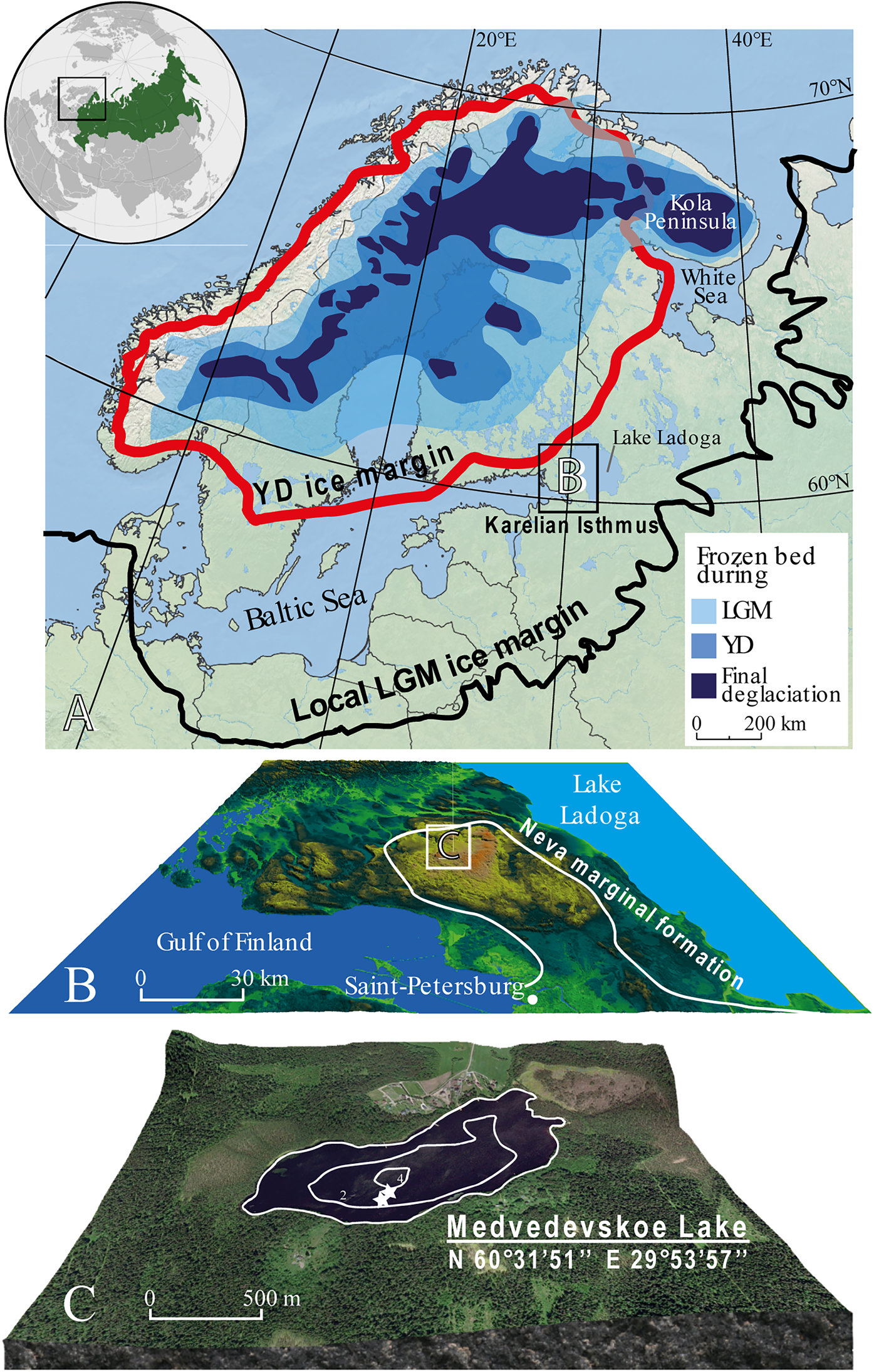
(color online) (A) The shrinkage of the Scandinavian Ice Sheet during deglaciation from its local last glacial maximum (LGM) position (Stroeven et al., Reference Stroeven, Hättestrand, Kleman, Heyman, Fabel, Fredin and Goodfellow2016); YD = Younger Dryas. (B) Map of the Karelian Isthmus (KI), position of the Neva marginal formation and location of Lake Medvedevskoe on the KI. (C) Lake Medvedevskoe; white stars show coring locations.
Here we present the results of a detailed study of sediments from Lake Medvedevskoe (LM), located on the central upland of the Karelian Isthmus (Fig. 1), using sediment structure, organic matter content, analysis of chironomids (Diptera: Chironomidae) and cladocerans (Crustacea: Branchipoda: Cladocera), and statistical models based on extensive databases of species composition and ecological parameters of the lakes from northern Russia (Nazarova et al., Reference Nazarova, Pestryakova, Ushnitskaya and Hubberten2008, Reference Nazarova, Herzschuh, Wetterich, Kumke and Pestjakova2011, Reference Nazarova, Self, Brooks, van Hardenbroek, Herzschuh and Diekmann2015). The main aims of our study are: (1) to trace the development of biological communities during the Holocene; and (2) to reconstruct qualitatively and quantitatively the palaeoecological conditions and palaeoclimate, respectively, of the Holocene on the Karelian Isthmus. Our findings are compared with regional data on the palaeoclimate of Fennoscandia to improve the understanding of Holocene changes in this region.
MATERIAL AND METHODS
Regional settings and sampling site
The Karelian Isthmus stretches between the Gulf of Finland, the Baltic Sea, and Lake Ladoga (Fig. 1). It is approximately 45–110 km wide and is located at the junction of the Baltic Crystaline Shield and the Russian Platform. The Isthmus can be divided into three landscape units: the lowland area in the north characterized by more than 800 lakes, the central highland, which reaches up to 203 m above sea level (asl), and the Neva Lowland (15–25 m asl) in the south. The Karelian Isthmus was strongly influenced by the Scandinavian Ice Sheet (SIS) during the Weichselian glaciation, and this has determined the heterogeneity of its geological structure and the variety of its landscapes (Subetto, Reference Subetto2009; Stroeven et al., Reference Stroeven, Hättestrand, Kleman, Heyman, Fabel, Fredin and Goodfellow2016). The last glacial maximum, known as the “Late Valday” glaciation in Russia, has recently been dated to 20.1 cal ka BP in northwestern Russia (Rinterknecht et al., Reference Rinterknecht, Hang, Gorlach, Kohv, Kalla, Kalm, Subetto, Bourlės, Lėeanni and Guillou2018). During this time, the ice margin reached the Valday region (~57°N, 34°E), ca. 350 km southeast of the Karelian Isthmus, and extended northwards towards the Barents Sea (Fig. 1A; Svendsen et al., Reference Svendsen, Astakhov, Bolshiyanov, Yu., Dowdeswell, Gataullin and Hjort1999).
The central part of the Karelian Isthmus is thought to have become deglaciated relatively early, prior to 15 cal ka BP, according to Gromig et al. (Reference Gromig, Wagner, Wennrich, Fedorov, Savelieva, Lebas, Krastel, Brill, Andreev, Subetto and Melles2019), although previous estimates were later (14.25–13.3 cal ka BP; Saarnisto and Saarinen, Reference Saarnisto and Saarinen2001). During deglaciation, the central part of the Karelian Isthmus formed a nunatak that rose above the surface of the glacier and featured small periglacial lakes (Subetto et al., Reference Subetto, Wohlfarth, Davydova, Sapelko, Wastegård, Possnert, Persson and Khomutova2002; Subetto, Reference Subetto2009). Hang (Reference Hang1997) and Hang et al. (Reference Hang, Subetto and Krasnov2000) revised Markov and Krasnov's (Reference Markov and Krasnov1930) varve-diagram correlations to show that the Isthmus became ice-free within a period of ca. 450 varve yr. Today, the region has a cool maritime climate, with a mean January temperature of -9°C, mean July temperature (T July) of + 16°C, and a mean annual temperature of + 3°C. Precipitation is around 600 mm/yr (Subetto, Reference Subetto2009).
The study site, LM (60°31.850′N, 29°53.950′E; 102.2 m asl), is located on the central highland within a hummocky moraine landscape at the outer margin of the Neva marginal formation (Fig. 1). LM was never flooded by larger water bodies following the deglaciation of the Karelian Isthmus.
Earlier studies have shown that the sediments of LM are represented by late-glacial grey sand and clay and Holocene dark-brown organic silt and contain a thin layer of Vedde volcanic ash dated at ca. 12.0 cal ka BP (Wastegård et al., Reference Wastegard, Wohlfarth, Subetto and Sapelko2000; Subetto, et al., Reference Subetto, Wastegård, Sapelko, Wohlfarth and Davydova2001). LM is characterized by a slow rate of continuous sedimentation, with allochthonous and aeolian components dominating the sediments (Subetto, Reference Subetto2009). Surrounding vegetation is dominated by Pinus sylvestris, Picea abies, dwarf shrubs, shrubs, lichens, and mosses (Subetto et al., Reference Subetto, Wohlfarth, Davydova, Sapelko, Wastegård, Possnert, Persson and Khomutova2002). LM has a surface area of ca. 0.46 km2, is 0.39 km wide and 1.22 km long, with a maximum depth of 4 m. The lake banks are low, sandy-stony, and loamy. The eastern and western shores merge into wetland. About 20% of the lake area is overgrown by macrophytes and vegetation extending from the shoreline. Algal blooms are not recorded (Andronikov et al., Reference Andronikov, Subetto, Lauretta, Andronikova, Rudnickaite, Drosenko and Syrykh2014). The ice-free period lasts from April to November (The National Atlas of Russia, 2006). LM is mesotrophic, fed and drained by small creeks, and the water column is unstratified (Subetto et al., Reference Subetto, Wohlfarth, Davydova, Sapelko, Wastegård, Possnert, Persson and Khomutova2002).
Fieldwork, geochemistry, and age model
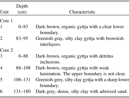
Two sediment cores, 0.95 and 1.8 m long, were collected from the ice in spring 2012 using a strengthened Russian corer (chamber length = 1 m, inside diameter = 5 cm). Core 1 was collected from a depth of 2.35 m and Core 2 was collected from a depth of 4 m. Organic content of the sediments was measured by loss on ignition (LOI, %) at 550°C (Heiri et al., Reference Heiri and Lotter2001; Ilyashuk and Ilyashuk, Reference Ilyashuk and Ilyashuk2007). Cores 1 and 2 were correlated to each other according to lithological marker horizons based on the LOI data and accelerator mass spectrometry (AMS) dates (Fig. 2, Table 1).
Core correlation. (A) Lithostratigraphies of Сores 1 and 2. (B) Results of the loss-of-ignition (LOI) analyses from Сores 1 and 2.

Radiocarbon ages and median of calibrated 14C ages in Cores 1 and 2 from Lake Medvedevskoe.
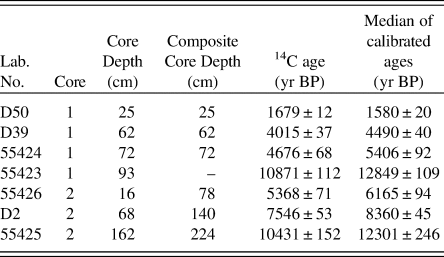
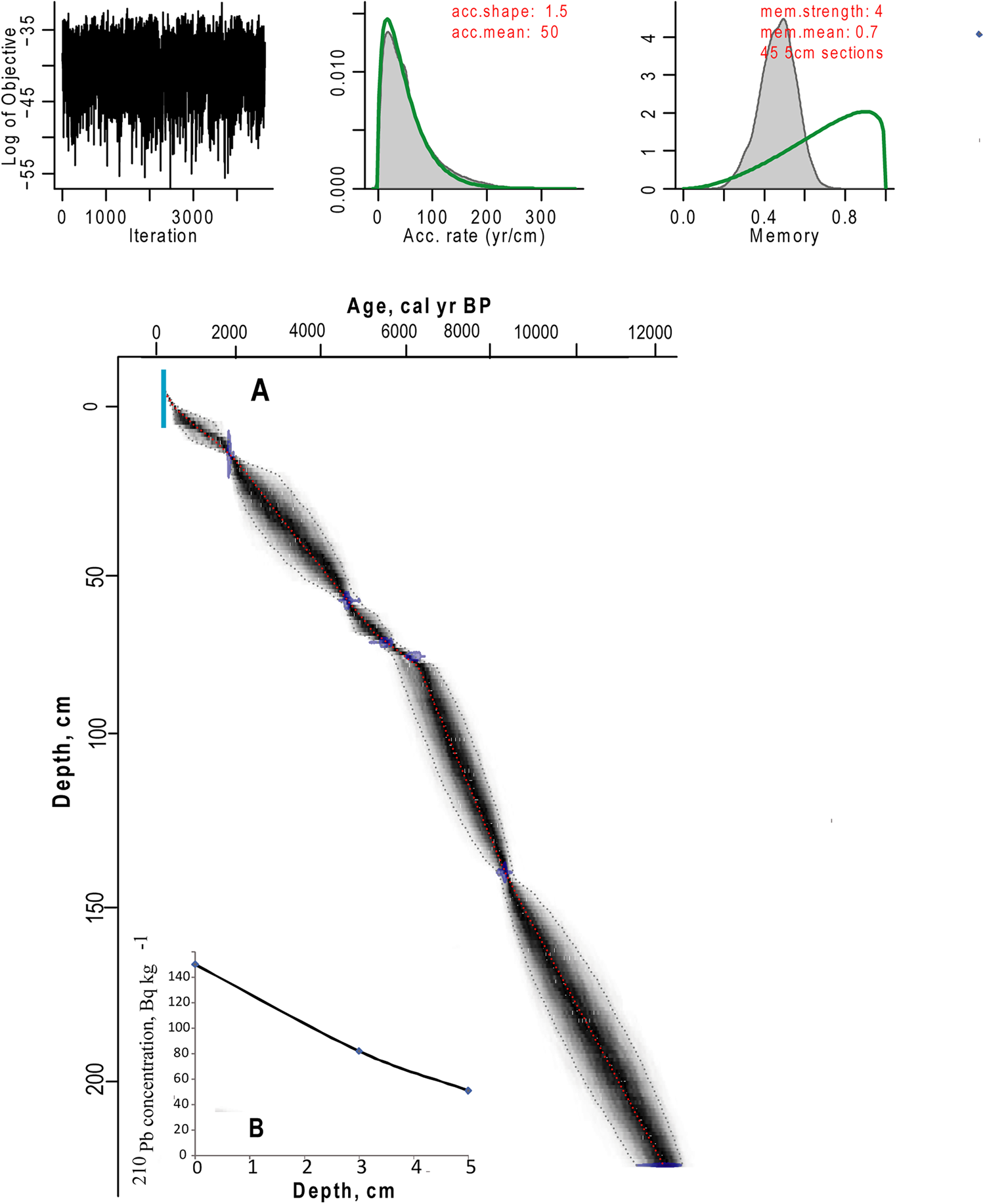
To construct an age-depth model, samples of bulk sediment were dated via AMS (Fig. 2, Table 1). Bulk material was used due to the lack of available plant material. The AMS radiocarbon dating of four samples (Lab. No. 5523–5526; Table 1) was performed in the Laboratory of Ion Beam Physics, Eidgenössische Technische Hochschule (ETH), Zürich. To increase the accuracy of the age model, further three samples were dated in the AMS Laboratory of Taiwan University (D2, D39, D50; Table 1). The uppermost sediment samples of both cores were analysed for 210Pb activity at the Geochronology Laboratory of St. Petersburg State University in order to obtain an additional time scale and control the upper radiocarbon chronology. 210Pb was found only in the upper sediment samples of Core 1, which provided evidence for the modern age of the upper part of Core 1. The topmost sediments of Core 2 were not retrieved (Fig. 2), and no 210Pb was recorded. The lower part of Core 1, between 74 and 93 cm, had a break in sedimentation (hiatus). Therefore, the upper part of Core 1 was combined with the preserved part of Core 2 to create a composite core for further palaeoecological analysis based on sedimentology and LOI. The lowermost date of Core 1 was omitted from the final age model, as this section of the core was not included in the composite core. The age-depth model (Fig. 3) was calculated with the Bacon 2.2 package (Blaauw and Christen, Reference Blaauw and Christen2011) for R software (R Core Team, 2012). The IntCal13 curve (Reimer et al., Reference Reimer, Bard, Bayliss, Beck, Blackwell, Bronk Ramsey and Buck2013), which is default in Bacon 2.2., was used to calibrate the AMS dates.
(color online) Age model. (A) Age-depth relationship of the combined core from LM. (B) Results of the 210Pb analysis of the upper 5 cm of Core 1.
Chironomids
Treatment of sediment samples for chironomid analysis followed standard techniques described in Brooks et al. (Reference Brooks, Langdon and Heiri2007). Chironomids were identified to the highest taxonomic resolution possible with reference to Wiederholm (Reference Wiederholm1983) and Brooks et al. (Reference Brooks, Langdon and Heiri2007). To capture the maximum diversity of the chironomid population, 59 to 118 chironomid larval head capsules were extracted from each sample. Several studies have demonstrated that this sample size is adequate for a reliable estimate of inferred temperature (Heiri and Lotter, Reference Heiri, Lotter and Lemcke2001; Larocque, Reference Larocque2001; Quinlan and Smol, Reference Quinlan and Smol2001). Information on the ecology of chironomid taxa was taken from Brooks et al. (Reference Brooks, Langdon and Heiri2007), Moller Pilot (Reference Moller Pillot2009), and Nazarova et al. (Reference Nazarova, Pestryakova, Ushnitskaya and Hubberten2008, Reference Nazarova, Herzschuh, Wetterich, Kumke and Pestjakova2011, Reference Nazarova, Self, Brooks, van Hardenbroek, Herzschuh and Diekmann2015, Reference Nazarova, Self, Brooks, Solovieva, Syrykh and Dauvalter2017a, Reference Nazarova, Bleibtreu, Hoff, Dirksen and Diekmann2017b).
Cladocera
Sediment samples were prepared for Cladocera analysis using the methods described in Korhola and Rautio (Reference Korhola and Rautio2001) and Frolova (Reference Frolova, Nazarova, Pestryakova and Herzschuh2013). The chitinous remains of cladocerans (headshields, shells, postabdomens, postabdomenal claws, and ephippia) were identified with reference to subfossil (Frey, Reference Frey1959, Reference Frey1973; Szeroczyńska and Sarmaja-Korjonen, Reference Szeroczyńska and Sarmaja-Korjonen2007) and modern (Flössner, Reference Flössner2000; Kotov et al., Reference Kotov, Sinev, Glagolev, Smirnov, Alexeev and Tsalolokhin2010) cladoceran identification keys. Because diverse parts are recorded, the most abundant body part was chosen for each species to represent the number of individuals. Between 88 and 285 individuals per sample were counted from each sub-sample. The percentages for all cladoceran species were calculated from this sum of individuals.
Numerical methods
Percentage stratigraphic diagrams were made in the program C2 version 1.7.7 (Juggins, Reference Juggins2007; Fig. 4 and 5). Zonation of stratigraphies was accomplished using the optimal sum-of-squares partitioning method (Birks and Gordon, Reference Birks, Gordon, Birks and Gordon1985) and the program ZONE (Lotter and Juggins, Reference Lotter and Juggins1991). The number of significant zones was assessed by a broken stick model (Bennett, Reference Bennett1996) using program BSTICK (Birks H.J.B. and Line J.M., unpublished). Species diversity was estimated using Hill's (Reference Hill1973) N2 index, which is commonly used as a measure of “effective” diversity, or a number of equally abundant species needed to obtain the same mean proportional species abundance as that observed in the dataset of interest (where all species may not be equally abundant).
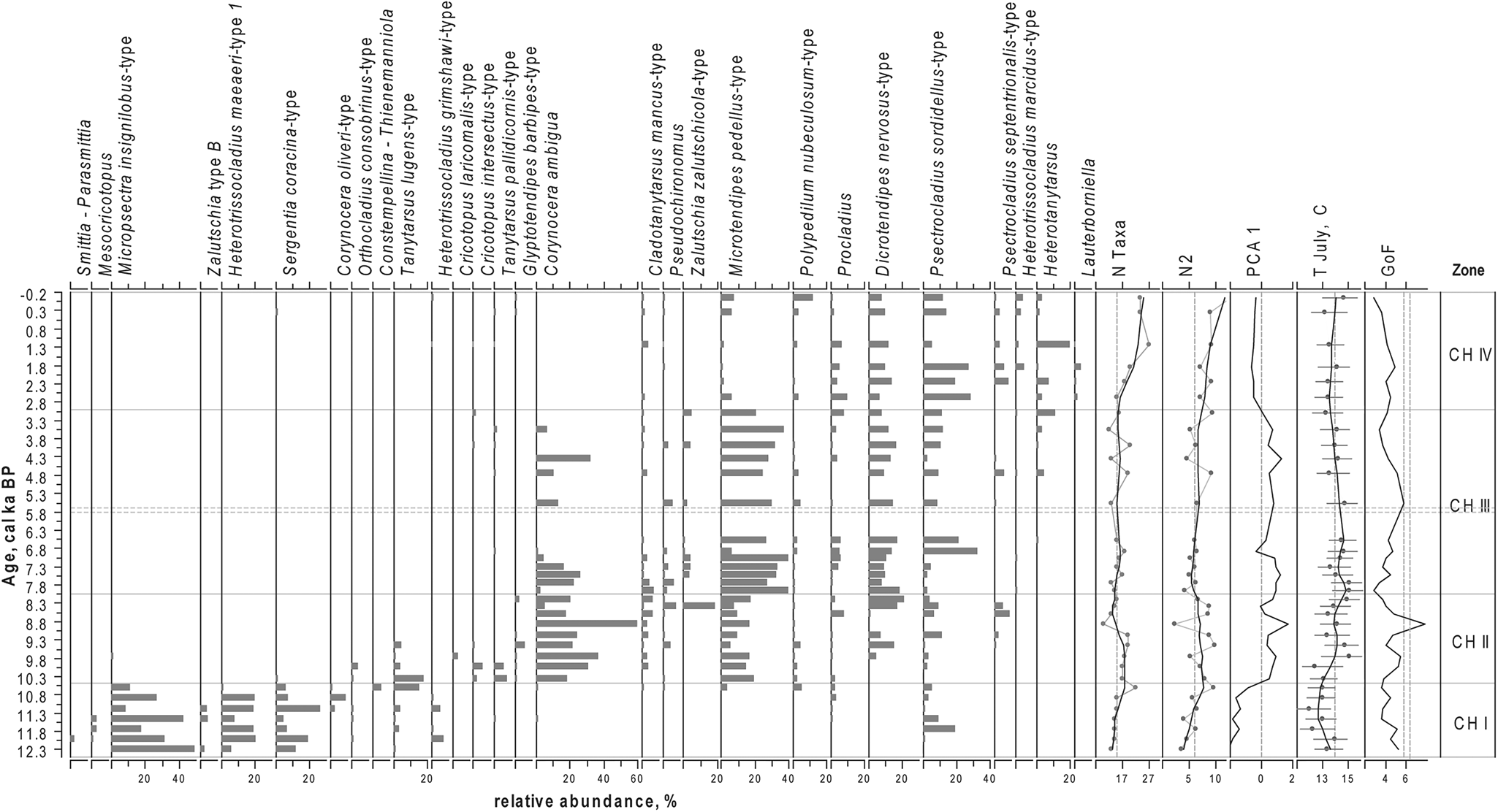
Relative proportions of the most abundant chironomid taxa in the sediments of Lake Medvedevskoe (LM), chironomid-inferred mean July air temperature (T July), PCA axes 1 scores for chironomid data, N2 diversity, number of chironomid taxa (N Taxa), and results of goodness-of-fit (GoF) tests for reconstructed T July, with 90th and 95th percentile of the residual distances of all the modern samples that are identified as samples with a “poor fit” and a “very poor fit” with the reconstructed T July, respectively (dashed lines). For taxon abundances, black lines represent a LOESS 0.2 smoothing of the data. For N2 and, N Taxa grey lines with dots represent the data and black lines represent a LOESS 0.2 smoothing of the data.
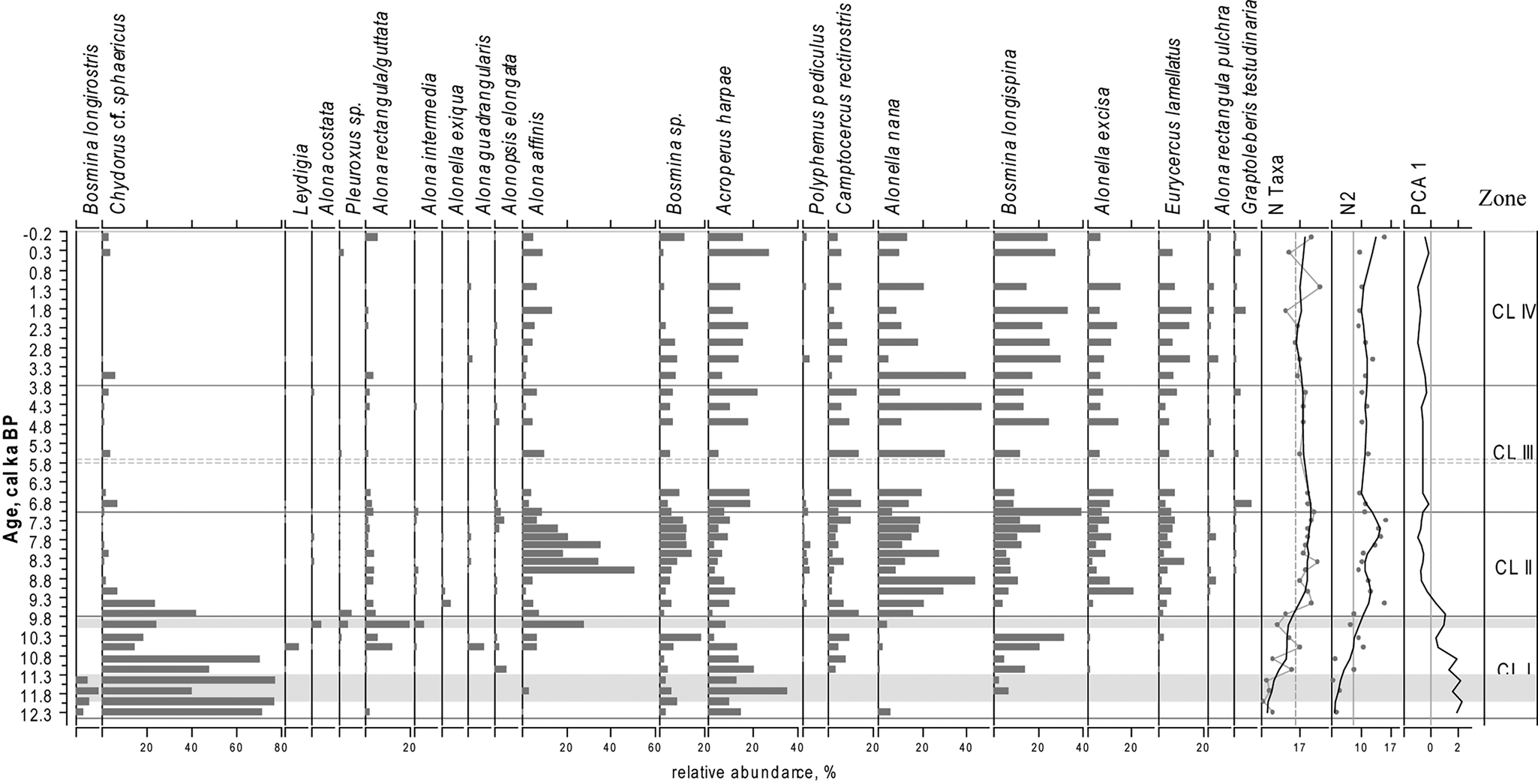
Relative proportions of the most abundant Cladocera taxa in the sediments of LM, PCA axes 1 scores for Cladocera data, N2 diversity, number of Cladocera taxa (N Taxa) of the Cladocera communities. For taxa abundances black lines represent a LOESS 0.2 smoothing of the data. For N2 and N Taxa grey lines with dots represent the data, black lines represent a LOESS 0.2 smoothing of the data. Grey areas represent layers with low concentration of cladoceran remains.
Detrended correspondence analysis (DCA), detrended by segments, was performed on the chironomid and cladoceran data (rare taxa downweighted) to determine the length of the sampled environmental gradients, from which we decided whether unimodal or linear statistical techniques would be most appropriate for the data analysis (Birks, Reference Birks, Maddy and Brew1995; Palagushkina et al., Reference Palagushkina, Nazarova, Wetterich and Shirrmaister2012, Reference Palagushkina, Wetterich, Schirrmeister and Nazarova2017). The gradient lengths of species scores were relatively short; the DCA axis 1 gradients were 1.58 standard deviation units for the chironomid data and 2.276 for the cladoceran data. This indicated that numerical methods based on linear response models are the most appropriate to assess the variation structure of the chironomids and cladoceran assemblages (ter Braak, Reference ter Braak, Jongman, ter Braak and van Tongeren1995). Principal component analysis (PCA) was used to explore the main pattern of taxonomic variations within the chironomid and cladoceran data throughout the sediment core (ter Braak and Prentice, Reference ter Braak and Prentice1988).
The quantitative air temperature reconstruction was based on calibration data sets of lakes from northern Russia (Nazarova et al., Reference Nazarova, Pestryakova, Ushnitskaya and Hubberten2008, Reference Nazarova, Herzschuh, Wetterich, Kumke and Pestjakova2011, Reference Nazarova, Self, Brooks, van Hardenbroek, Herzschuh and Diekmann2015, Reference Nazarova, Self, Brooks, Solovieva, Syrykh and Dauvalter2017a). T July temperatures were inferred by using a North Russian (NR) chironomid-based temperature inference model (WA-PLS, 2 component; R 2 boot = 0.81; RMSEP boot = 1.43°C) based on a modern calibration dataset of 193 lakes and 162 taxa from northern Russia (61–75°N, 50–140°E, T July range = 1.8 to 18.8°C; Nazarova et al., Reference Nazarova, Self, Brooks, van Hardenbroek, Herzschuh and Diekmann2015). T July for the lakes in the calibration dataset was derived from a climatic dataset compiled by New et al. (Reference New, Lister, Hulme and Makin2002). The T July NR model has been previously applied for palaeoclimatic inferences in Siberia and European northern Russia and demonstrated high reliability of reconstructed parameters (Kienast et al., Reference Kienast, Wetterich, Kuzmina, Schirrmeister, Andreev, Tarasov, Nazarova, Kossler, Frolova and Kunitsky2011; Solovieva et al., Reference Solovieva, Klimaschewski, Self, Jones, Andrén, Andreev, Hammarlund, Lepskaya and Nazarova2015; Diekmann et al., Reference Diekmann, Pestryakova, Nazarova, Subetto, Tarasov, Stauch and Thiemann2016).
Chironomid-based reconstructions were performed in C2 version 1.7.7 (Juggins, Reference Juggins2007). The species data were square-root transformed to stabilise species variance. To assess the reliability of the chironomid-inferred T July reconstruction, we calculated the percentage abundances of the fossil chironomids that are rare or absent in the modern calibration data set. A taxon is considered to be rare in the modern data when it has a Hill's N2 (Hill, Reference Hill1973) value below five. The temperature optima of the taxa that are rare in the modern dataset are likely to be poorly estimated (Brooks and Birks, Reference Brooks and Birks2001).
A goodness-of-fit statistic (GoF), derived from a canonical correspondence analysis (CCA) of the modern calibration data and down-core passive samples with T July as the sole constraining variable, was used to assess the fit of the analysed down-core assemblages to the reconstructed T July (Birks et al., Reference Birks, Line, Juggins, Stevenson and ter Braak1990; Birks, Reference Birks, Maddy and Brew1995, Reference Birks1998). This method shows how unusual the fossil assemblages are in respect to the composition of the training set samples along the temperature gradient. Fossil samples with a residual distance to the first CCA axis larger than the 90th and 95th percentile of the residual distances of all the modern samples were identified as samples with a “poor fit” and a “very poor fit,” respectively, with the reconstructed T July (Birks et al., Reference Birks, Line, Juggins, Stevenson and ter Braak1990).
PCA and CCA were performed using CANOCO 4.5 (ter Braak and Šmilauer, Reference ter Braak and Šmilauer2002). Chironomid percentage data were square-root transformed and rare taxa were downweighted. In the evaluation of GoF, the CCA scaling focused on inter-sample distances with Hill's N2 scaling selected to optimise inter-sample relationships (Velle et al., Reference Velle, Brooks, Birks and Willasen2005).
DCA was run on the square-root transformed LM temporal chironomid and cladoceran sequences, using the vegan package in R (Oksanen et al., Reference Oksanen, Blanchet, Friendly, Kindt, Legendre, McGlinn and Minchin2017), and the DCA scores were analysed for breakpoints, using the strucchange package in R (Zeileis et al., Reference Zeileis, Leisch, Hornik and Kleiber2002, Reference Zeileis, Kleiber, Kraemer and Hornik2003). The DCA axis 1 scores for the composite core were compared to DCA axis 1 scores calculated independently for Core 1 and 2, for both the chironomid and cladoceran data, in order to additionally test the acceptability of merging the taxa datasets from Core 1 and 2 into a composite assemblage.
Community composition change was explored using species richness, species diversity (Hill's N2) and compositional disorder (°disorder) analyses for the temporal chironomid and cladoceran assemblages, following Doncaster et al. (Reference Doncaster, Chávez, Viguier, Wang, Zhang, Dong, Dearing, Langdon and Dyke2016). Compositional disorder allows the species assemblages to be analysed further by investigating how the community composition is changing, and whether this is in a linear, predicable manner, or an unstructured, disordered manner, which may be indicative of an approaching critical transition (Doncaster et al., Reference Doncaster, Chávez, Viguier, Wang, Zhang, Dong, Dearing, Langdon and Dyke2016). Compositional disorder is measured on a continuous scale similar to temperature, with 0° indicating a highly ordered, completely nested community, wherein the species assemblage is a subset of the previous one and is therefore predictable. A highly disordered species composition has a value of 100°, indicating a completely unnested community where the species composition is unpredictable due to a lack of common species (Rodriguez-Girones and Santamaria, Reference Rodriguez-Girones and Santamaria2006; Doncaster et al., Reference Doncaster, Chávez, Viguier, Wang, Zhang, Dong, Dearing, Langdon and Dyke2016). °Disorder was calculated using a 10-point subset, where the calculation for one data point included the following nine data points, hence °disorder values are not available for the lower 9 data points.
RESULTS
Lithology, geochemistry, and age model
In the lithological structure of Core 1, two sediment units can be distinguished: a dark-brown organic 83-cm-thick gyttja (unit 1; Fig. 2A) and a 12-cm-thick, greenish-grey, layered, silty clay gyttja (unit 2). The lithological structure of Core 2 was similar, with the upper 108 cm of the core consisting of organic gyttja (units 3 and 4), of which the lower 20 cm had weak lamination (unit 4). Unit 5 of Core 2 (23 cm thick) was similar to unit 2 of Core 1 and was also represented by greenish-grey, silty clay gyttja. The lowermost unit 6 consisted of dark-grey, dense, silty clay with admixed sand.
Results of the LOI analysis demonstrated complimentary trends across the two cores. The LOI values gradually increased from 4–6% at the lowermost parts of Core 2, with up to 87% at the central, overlapping sections and the upper section of Core 1 (Fig. 2B).
The 14C results from both Core 1 and 2 show that the dates are in chronological order (Fig. 2, Table 1). We spliced the upper 72 cm of Core 1 at 28 cm core depth of the remaining part of Core 2, where both records had identical LOI values, the closest obtained 14C dates and the modelled ages based on AMS dates showed similar ages (Fig. 2 and 3, Table 2). Further support for the chosen splicing approach and the resulting age model was obtained from the DCA analysis of the biological assemblages of both Core 1 and 2 (SOM 1; Fig. 1 and 2). A large degree of overlap in the DCA scores for axes 1 and 2 for Core 1 and 2 (SOM 1; Fig. 1 and 2) suggests broadly similar taxonomic compositions within the two cores at the chosen splicing position. As LM has a simple bathymetry, merging the datasets to create a composite core is not unreasonable. The resulting composite core was 224 cm long and covered a time interval from ca. 12.3 cal ka BP to the present-day (Fig. 3, Table 1).
Lithostratigraphic description of the sediment cores from Lake Medvedevskoe.
Chironomids
In total, we identified 82 chironomid taxa. The down-core changes in the chironomid assemblages led to the identification of four statistically significant zones (CH I–IV; Fig. 4).
CH I (ca. 12.3–10.5 cal ka BP)
Species richness is low. The N2 diversity varies from 3.5 to 6.5 and increases to 9.0 at the top of this zone (ca. 10.6 cal ka BP). Chironomid faunas are dominated by cold-stenothermic taxa characteristic of oligotrophic conditions, such as Micropsectra insignilobus-type and Sergentia coracina-type, and by Heterotrissocladius maeaeri-type 1, which is indicative of moderate temperature conditions. In this zone, a number of less abundant, cold oligotrophic indicators occur: Corynocera oliveri-type, Zalutschia type B, Mesocricotopus, and Heterotrissocladius grimshawi-type. The abundance of Tanytarsus lugens-type, a cold-stenothermic, profundal taxon, increases towards the top of the zone, indicating a possible lake deepening at this time. In this zone, a combination of acidophilic (Heterotrissocladius, S. coracina-type, Mesocricotopus, and Psectrocladius sordidellus-type) and acidophobic (M. insignilobus-type) taxa alternate in dominance.
CH II (ca. 10.5–8.0 cal ka BP)
Throughout this zone, N2 diversity remains around 8.1, with the highest taxonomic richness between ca. 9.5 and 8.3 cal ka BP. A strong decline in N2 values and species richness occurs at ca. 8.9 cal ka BP, when the dominant taxon in this zone, Corynocera ambigua, constitutes 64% of the chironomid fauna. Sublittoral/littoral taxa characteristic of warmer conditions and associated with macrophytes prevail: C. ambigua, Microtendipes pedellus-type, Dicrotendipes nervosus-type, Zalutschia zalutschicola-type, and Cladotanytarsus mancus-type.
CH III (ca. 8.0–3.0 cal ka BP)
N2 diversity is slightly lower in this zone (median 6.1). C. ambigua gradually declines and the fauna is dominated by M. pedellus-type, with high abundancies of meso- to eutrophic taxa: D. nervosus-type, P. sordidellus-type, and Procladius.
CH IV (ca. 2.9 cal ka BP–present time)
This period is characterized by the highest taxonomic richness and diversity (N2 median of 9.3) and a strong taxonomic shift: C. ambigua disappears from the fauna and M. pedellus-type declines. The chironomid fauna is dominated by D. nervosus-type, P. sordidellus-type, Procladius, and several other eutrophic and acidophilic taxa, including Heterotanytarsus, Psectrocladius septentrionalis-type, Heterotrissocladius macridus-type, and Lauterborniella.
Cladocera
Throughout the LM core, a total of 38 cladoceran taxa were found, belonging to seven families: Bosminidae, Holopedidae, Chydoridae, Daphnidae, Polyphemidae, Macrotricidae, and Sididae. Both pelagic and littoral taxa are well represented in the lake and the cladoceran communities are dominated by Chydoridae (75.28%) and Bosminidae (22.67%) species. The LM cladoceran stratigraphic diagram (Fig. 5) is subdivided into four statistically significant stratigraphic zones (CL I–IV; Fig. 5).
CL I (ca. 12.3–9.8 cal ka BP)
The cladoceran communities in this zone are characterized by the lowest N2 indices in the record and dominance of typical arctic Cladocera species (Acroperus harpae, Chydorus cf. sphaericus, and Bosmina (Eubosmina) longispina). Between ca. 12.0 and 11.3 and around ca. 9.9 cal ka BP, only a few cladoceran remains were found. This part of the core is marked in grey in Figure 5. The average value of N2 diversity in CL I is 5.5. This period is characterized by a strong dominance of cosmopolitan Chydorus cf. sphaericus (Flössner, Reference Flössner2000; Frolova et al., Reference Frolova, Nazarova, Pestryakova and Herzschuh2013, Reference Frolova, Nazarova, Pestryakova and Herzschuh2014, Reference Frolova, Nazarova, Zinnatova, Frolova and Herzschuh2017a), which decreases in abundance towards the upper levels of the zone. The subdominant species Arcoperus harpae and Chydorus cf. sphaericus are typical and often dominant species in modern northernmost arctic lakes and ponds (Frolova, L., personal communication, 2019). The second part of the period is marked by increases in oligosaprobic, planktonic taxa that are typical of cold-water Bosmina (Eubosmina) longispina (Frolova, Reference Frolova2016; Frolova et al., Reference Frolova, Ibragimova, Ulrich and Wetterich2017b).
CL II (ca. 9.8–7.1 cal ka BP)
The mean value of N2 increases to 14.6. There are significant changes in the composition of subfossil cladoceran communities connected with an increase in species indicative of changing environmental and climatic conditions. C. cf. sphaericus (Fig. 5) declines and nearly disappears from the record after 9.1 cal ka BP. Remains of the predatory Polyphemus pediculus are common during this period. The abundance of B. (E.) longispina slightly decreases at the bottom of the zone and increases again towards the top.
CL III (ca. 7.1–3.8 cal ka BP)
The average value of N2 diversity declines to 9.3. There is a sharp decrease in the number of relatively large phytophilic A. affinis that dominated CL II as well as a simultaneous increase in A. nana, a small vegetation dweller. Proportions of A. harpae, Camptocercus rectirostris, and Graptoleberis testudinaria increase compared with the previous zone.
CL IV (ca. 3.8 cal ka BP–present time)
The average value of N2 diversity index decreases further to 8.6. The zone is characterized by a decline in A. nana. At the same time, the pelagic B. (E). longispina became dominant again. There was also an increase in abundances of Eurycercus sp. and A. affinis.
Community composition
The trends seen in the species richness, Hill's N2 diversity and DCA axis 1 scores are similar for the chironomid and cladoceran communities: DCA axis 1 scores show a shift in community composition during the early Holocene development of the ecological system in LM (Fig. 6). Breakpoint analyses identified statistical breaks in the DCA axis 1 scores at 3.12, 9.17, and 10.60 cal ka BP in the chironomid community, and at 9.17 and 10.60 cal ka BP in the cladoceran community, suggesting significant shifts in the species present at these intervals.
Species richness (green, dot-dashed line), Hill's N2 diversity (blue, dashed line), compositional disorder (red, dotted line) and DCA axis 1 scores (black, solid line), plotted against time for the chironomid and Cladocera species communities. The vertical dotted lines represent statistically calculated breakpoints in the DCA axis 1 scores at 3.12, 9.17, and 10.60 cal ka BP in the chironomid community, and at 9.17 and 10.60 cal ka BP in the Cladocera community. Stratigraphic zones identified within the chironomids and Cladocera zones are displayed in pale blue-grey. (For interpretation of the references to color in this figure legend, the reader is referred to the web version of this article.)

The chironomid community shows a high level of °disorder (44–46°) during the early Holocene, while the Cladocera community appears more organised at this point, with °disorder values of 15–23°. Between ca. 6.7 and 2.9 cal ka BP, approximately corresponding to the middle Holocene, the chironomid and cladoceran communities display a long period of stable community conditions (°disorder values between ca. 30–37°). During the late Holocene (ca. 2.9 cal ka BP to present), °disorder declines to values of 28–23°.
Reconstruction of the mean July air temperature (T July)
Reconstructed T July fluctuates by approximately 3°C over the last ca. 12.3 ka (Fig. 4). The main variation shows temperatures being lowest (median T July 12.9°C) in the period between ca. 11.7 and 10.3 cal ka BP and highest between ca. 9.7 and 5.5 cal ka BP (for this interval, median T July = 14.5°C, max T July = 15.1°C). Temperatures fluctuate within the generally warm early Holocene, with lower values ca. 8.5–8.1 and ca. 7.3–6.8 cal ka BP. From ca. 5.5 to 0.1 cal ka BP there was a gradual cooling of temperature (median T July = 13.5°C). T July in the modern sample is reconstructed as 14.8°C, which is similar to the modern T July (16°C), taking into account the RMSEP of the applied model (1.43°C).
All dominant taxa in the fossil record are well represented (N2 > 5) and all 82 identified chironomid taxa were represented in the modern training sets. Eight of the 82 taxa had a Hill's N2 < 5 and therefore are defined as not well represented in the training sets: Einfeldia pagana-type, Harnischia, Hydrobaenus johannseni-type, Paracladopelma, and Stenochironomus Xenochironomus. These taxa appear in the record once each. Lauterborniella appears in three samples in CH IV at abundances of 0.8–1.6% and once at an abundance of 3.7% at ca. 1.8 cal ka BP. All these seven taxa are rare in the record, appear at low abundances, and therefore do not influence the reconstruction. GoF statistics for T July reconstruction reveal that only one sample has a “poor” fit with temperature (Fig. 4). In this sample (ca. 8.9 cal ka BP), the chironomid fauna is strongly dominated by C. ambigua (64%). The rest of the samples show a “good fit” with temperature (see Materials and Methods). The high representation of the taxa in the training set, together with mostly good GoF statistics results, indicates that the temperature reconstruction from the LM records is reliable.
DISCUSSION
The analysis of fossilized biological remains from the sediments of LM, at the southeastern edge of Fennoscandia, gives an insight into changes in chironomids and cladoceran communities since the late Pleistocene. This provides an opportunity to infer the paleoclimate and lake-basin development, and, by comparison our data with information available from other parts of Fennoscandia, our results can be placed into a broader geographical context.
Faunal changes
In both the chironomid and cladoceran communities, we observed several phases with clearly expressed dominant species. Taxonomic richness of biological communities was low at the base of the core and generally increased towards the sediment surface, along with organic content (LOI). In the Cladocera communities, the most prominent taxonomic shift coincided with an increase in organic matter concentration between ca. 10.6 and 9.1 cal ka BP. At this time, cold-water littoral (Ch. cf. sphaericus and A. harpae), tolerant to oxygen variations (Ch. cf. sphaericus) and planktonic cold-water oligosaprobic taxa (B. [E.] longispina) were replaced by fauna typically associated with submerged vegetation (Alona, Alonella, and Eurycercus sp.). In the chironomid communities, cold stenotherms, such as M. insignilobus-type, H. maeaeri-type, and S. coracina-type, dominated the record before 10.5 cal ka BP, indicating cold climatic conditions and an input of cold thawing waters from surrounding area.
Between ca. 10.4 and 7.3 cal ka BP, the chironomid C. ambigua was dominant, with a high abundance of M. pedellus-type. Between ca. 7.3 and 3.1 cal ka BP, M. pedellus-type dominated with C. ambigua present (Fig. 4). M. pedellus-type is a known indicator of oligomesotrophic lakes (Brodersen et al., Reference Brodersen, Dall and Lindegaard1998), can tolerate slight acidification (Moller Pillot, Reference Moller Pillot2009), and is rarely found under eutrophic conditions (Langdon et al., Reference Langdon, Ruiz, Brodersen and Foster2006). C. ambigua proliferated during the Late Glacial in northern Europe at low temperatures in lakes with silty and largely inorganic sediments, abundant oxygen, and probably extensive charophyte beds in transparent, carbonate-rich waters (Brodersen and Lindegaard, Reference Brodersen and Lindegaard1999). With climatic amelioration, extensive erosion, and redeposition of lake sediments (Digerfeldt, Reference Digerfeldt and Berglund1986; Nazarova et al., Reference Nazarova, Lüpfert, Subetto, Pestryakova and Diekmann2013a) and an increase in nutrient availability could have led to an outward spread of aquatic macrophytes (Digerfeldt, Reference Digerfeldt and Berglund1986) and a change from a “Chara” to “Potamogeton lake” (Forsberg, Reference Forsberg1965); this might have contributed to the reduction in C. ambigua populations in northern Europe and in LM.
Similar C. ambiqua/M. pedellus-type stages (CH II; Fig. 4) have been found in several sites around the region, where high abundancies of these two taxa coincided with periods of increasing organic matter content in sediments, representing a transition from oligotrophic to oligomesotrophic or mesotrophic states during the early Holocene. In southern Finland, this stage occurred earlier, from ca. 11.5 to 10.5 cal ka BP (Luoto et al., Reference Luoto, Kultti, Nevalainen and Sarmaja-Korjonen2010), and C. ambigua remained present until 7.5 cal ka BP. In northeastern Fennoscandia, on the Kola Peninsula and on the Karelian Isthmus (LM), the C. ambiqua/M. pedellus-type stage was delayed. In the north of the Kola Peninsula it lasted until ca. 9.6 cal ka BP (Ilyashuk et al., Reference Ilyashuk, Ilyashuk, Kolka and Hammarlund2013) and in the south of the Kola Peninsula it appeared simultaneously with the Karelian Isthmus (LM): from ca. 10.0 to 8.0 cal ka BP (Ilyashuk et al., Reference Ilyashuk, Ilyashuk, Hammarlund and Larocque2005).
Biological communities in the last ca. 3 ka became progressively diverse and both cladoceran and chironomid faunas included mostly phytophilic and acid-tolerant taxa, presumably in response to further changes, including lake paludification.
Shifts in taxonomic composition are mirrored by the results of species richness and diversity analyses; breakpoints identified in the DCA axis 1 scores coincide with an increase in species richness and diversity for both chironomids and Cladocera (Fig. 6). The breakpoints do not directly match the boundaries between the CH and CL zones but indicate considerable changes in the composition of biological communities around these boundaries.
The time series plot of compositional disorder (°disorder), species richness and species diversity (Fig. 6) shows gradual changes in the species community composition over time. The rise in species richness and diversity are parallel, signifying an increase in the evenness of the distribution of species abundance in connection with the rising number of species. While species richness and diversity provide information about the number of species present and their abundance, °disorder can help infer information about the orderliness of species loss or gain. Higher °disorder values indicate more disorder in the species turnover. On a broad time scale, increases in species richness and diversity correlate with lower °disorder values, showing, for a given time period, the community composition had many species in common with the previous time slice and was therefore developing in a predictable manner.
While species richness and diversity rise gradually over time in the chironomid and Cladocera assemblages as expected in a developing ecosystem, the °disorder scores suggest opposing results for the Cladocera and chironomid communities during the early Holocene. The high °disorder values in the chironomid community suggest that there was a large turnover of species and few common species between samples, in keeping with an ecosystem reacting to a developing environment following deglaciation (Subetto et al., Reference Subetto, Wohlfarth, Davydova, Sapelko, Wastegård, Possnert, Persson and Khomutova2002). In these early stages (12.0 to 9.0 cal ka BP), species richness is relatively low, between 13–22 species. The chironomid assemblage diagram also shows a number of species with a fluctuating presence during this period (Fig. 4). In contrast, the early-stage cladoceran communities have lower values of °disorder, despite species richness showing greater variation (4–21 species; Fig. 5 and 6). This suggests that there were fewer species lost and a more ordered community development.
The opposing °disorder values seen in the chironomid and Cladocera assemblages can be explained by the variables that influence the organisms’ presence. Chironomid species react to changes in July air temperature (Brooks et al., Reference Brooks, Langdon and Heiri2007; Nazarova et al., Reference Nazarova, Self, Brooks, van Hardenbroek, Herzschuh and Diekmann2015); these were often more developed in the early Holocene, when the climate was undergoing widespread change. Cladocera are more indicative of water variables, such as phosphorus (Lotter et. al., Reference Lotter, Birks, Hofmann and Marchetto1998), lake depth (Korhola, Reference Korhola1999), and water temperature (Frolova et al., Reference Frolova, Nazarova, Pestryakova and Herzschuh2014). The high °disorder values in the chironomid data could indicate that the surrounding terrestrial environment was still highly variable in the early Holocene. In contrast, the aquatic environment of LM may have undergone greater development during the middle Holocene period, where Cladocera °disorder values were highest.
Species richness and biodiversity have been highest in the most recent period, ca. 2.9 cal ka BP to present, when °disorder is also at its lowest. The different time slices have more species in common, suggesting less turnover of species in association with a more stable wider environmental system in recent time.
Palaeoclimate and lake-basin development
Trends in the organic matter content of the sediment and biological community composition provide a reconstruction of climate and lake catchment development from the Pleistocene/Holocene boundary to modern time. Qualitative patterns of change, together with the chironomid-based T July reconstruction, demonstrate that the lake ecosystem was highly responsive to large-scale climatic forcing during the Holocene.
Late Pleistocene / Holocene transition (12.3–10 cal ka BP)
The lower part of the core (Fig. 2–6) clearly represents the initial stage of the formation of LM during the beginning of deglaciation. Sediments from this time interval are dark-grey, dense, silty clay with admixed sand and very low organic matter content. Biological communities were poor, with low taxon richness and diversity and cold-stenothermic oligotrophic taxa dominating. During this time, Chydorus cf. sphaericus, a pioneering, eurytopic, highly adaptive species, was abundant. This is ecologically flexible species that can withstand varying levels of dissolved oxygen. It is a nearshore (littoral) organism with limited swimming abilities, most commonly found clinging to various filamentous algae with its modified limbs (Fryer, Reference Fryer1968). Chydorus cf. sphaericus is generally found in lakes on or near the bottom sediments. Another abundant species, Acroperus harpae, is a common inhabitant of the littoral areas of lakes and other small water bodies. It is most frequently found in association with vegetation, although occasionally it can be found on bare rocky shores or sand (Fryer, Reference Fryer1968). Paleolimnological studies show that A. harpae is an indicator of cold temperatures (Kattel and Sirocko, Reference Kattel and Sirocko2011). During this time interval, highest abundances of the acidophobic M. insignilobus-type were accompanied by declines in acidophilic taxa, and vice versa (Fig. 4). This probably reflects fluctuations in water depth and variation in the development of the macrophytes in the littoral zones.
The dominance of a cold-stenothermic fauna with the presence of semiaquatic chironomid taxa (Smittia-Parasmittia), which can tolerate variations in oxygen saturation, and alternating dominance of acidophilic and acidophobic taxa further indicate the instability of lacustrine conditions and, probably, erosion of the lake shore during the initial stages of lake formation. Variations in lake depth and water chemistry might also have resulted from the amount and intensity of thawed water supply; this probably caused waterlogging of the shoreline zone of the lake and affected the intensity of humic acid input from surface runoff in the drainage area (Subetto et al., Reference Subetto, Davydova, Sapelko, Wohlfarth, Wastegård and Kuznetsov2003; Wohlfarth et al., Reference Wohlfarth, Lacourse, Bennike, Subetto, Tarasov, Demidov, Filimonova and Sapelko2007).
Mean July temperatures at this time, as inferred from the chironomid record of LM (Fig. 4) were 3–4°C below modern level. Earlier studies have shown that before ca. 12.65 cal ka BP, the climate on the Karelian Isthmus was arctic, cold, and dry (Subetto et al., Reference Subetto, Davydova, Sapelko, Wohlfarth, Wastegård and Kuznetsov2003). In summer, the lake received water from the nearby glacier and melting blocks of dead ice, causing active mixing of the water column and alkalizing the water. Summer seasons were short and the lake was probably not ice-free every year. LM was shallow, poorly populated by benthic diatoms and surrounded by a treeless landscape. Tundra vegetation dominated the lake vicinity until ca. 11.5 cal ka BP and was replaced by birch forests thereafter (Subetto et al., Reference Subetto, Wohlfarth, Davydova, Sapelko, Wastegård, Possnert, Persson and Khomutova2002). The change in vegetation probably indicated a change in moisture availability as well as temperature: a dry, cold climate was replaced by more humid and warmer conditions. After ca. 11.0 cal ka BP, the last areas of dead ice disappeared, birch-pine forests spread, and a more fertile soil cover began to form. Lake water pH began to shift from alkaline to acidic due to increasing input of humic acids from the forested catchment areas. The increase in available moisture led to a rise of the lake level around ca. 10.6 cal ka BP; this inference is supported by the increase in abundance of the profundal T. lugens-type. At ca. 10.0 cal ka BP it declined, however, indicating a possible lake-level lowering.
Between ca. 10.6 and 10.0 cal ka BP significant changes occurred in the lake's biological communities, following a gradual increase in the content of organic carbon in the bottom sediments (Fig. 2). The rising concentration of organic matter in the sediments (deposition of gyttja) reflects an increase in the productivity of the lake, while input of allochthonous mineral matter from the catchment decreased due to the development of vegetation and soil cover around the lake. After ca. 10.2 cal ka BP, pine, elm, and grey alder appeared in the forests around the lake, and Poaceae and Cyperaceae dominated grass communities (Subetto, Reference Subetto2009). The hazel and elm likely migrated to the Karelian Isthmus from the west, where they have been previously reported at 10.7 cal ka (Saarse et al., Reference Saarse, Mäemets, Pirrus, Rõuk, Sarv, Ilves, Berglund, Birks, Ralska-Jasiewiczowa and Wright1996).
Early Holocene (10–8 cal ka BP)
Reconstructed T July showed a steady warming trend that was interrupted by a slight decline between ca. 8.5 and 8.1 cal ka BP, with a value of 13.2°C at ca. 8.2 cal ka BP (Fig. 4). This short cooling at ca. 8.2 cal ka BP may be associated with “Finse Event” or “8.2 cal ka event” (Alley et al., Reference Alley, Mayewski, Sowers, Stuiver, Taylor and Clark1997; Nesje and Dahl, Reference Nesje and Dahl2001). In response to climate amelioration, the diversity of biological communities grew, while cold-stenothermic chironomid taxa declined and were replaced by C. ambigua and other taxa characteristic of mesotrophic conditions (Fig. 4 and 5). Cladocera species associated with higher trophic conditions appeared, and there was a sharp decline in the cold-water oligosaprobic taxon B. (E.) longispina, further supporting reconstructed from chironomids temperature increase.
Typical littoral taxa and epiphytes constitute the majority of the cladoceran communities: Alona (A. affinis and A. rectangula/guttata), Alonella (A. excisa and A. nana), and Eurycercus sp. A. excisa and A. nana are commonly recorded in and between Sphagnum plants and A. excisa also occurs in acid waters (Fryer, Reference Fryer1968). Shifts in the biological communities and organic content of the sediment indicate that during the early Holocene the lake was well oxygenated, with high water transparency, as indicated by the presence of C. ambigua.
Middle Holocene (8–4 cal ka BP)
During this interval, the organic content of the sediments was the highest in the record, indicating the growing productivity of the lake ecosystem (Fig. 2). In the biological communities, the abundance of littoral and phytophilic Cladocera species (A. nana and A. excisa) and the proliferation of chironomid taxa (M. pedellus-type, D. nervosus-type, and Procladius) indicate a moderately warm climate (Fig. 4 and 5). At this time, C. ambigua gradually declined. This was probably due to an increase in biological productivity in LM as a result of climatic amelioration (Digerfeldt, Reference Digerfeldt and Berglund1986).
Between ca. 8.9 and 7.5 cal ka BP, a change in the dominant cladoceran species from a small A. nana to a large sized A. affinis indicates a shift towards K-selected species that typify stable or predictably developing environments (Odum, Reference Odum1963). After ca. 7.5 cal ka BP, large phytophilic A. affinis declined, while A. nana, which is a more flexible pliable vegetation dweller, increased. A. nana has a wider distribution and can tolerate different types of water bodies; from oligo- to eutrophic (Nevalainen, Reference Nevalainen2008; Smirnov, Reference Smirnov2010). There is some evidence that this species can tolerate acidic conditions (Fryer, Reference Fryer1968; however, Sandøy and Nilssen [Reference Sandøy and Nilssen1986] disagree). These changes in the taxonomic composition of Cladocera, which include an increase of the phytophilic and acid-tolerant taxa, may indicate a decrease in stability of ecological conditions in the lake, particularly as there is an increase in the odisorder of the cladoceran communities after ca. 7.5 cal ka BP. After ca. 7.9 cal ka BP, at the time when the reconstructed T July reached its highest values, it is likely that the lake littoral areas were overgrown by macrophytes, which, particularly under warm conditions, would encourage paludification processes and possible oxygen depletion.
The reconstructed temperatures were the highest in the record during the middle Holocene period (Fig. 4). Based on this record, the period between ca. 9.5 and 5.5 cal ka BP represents the Holocene thermal maximum (HTM) in the region, with the warmest period centered at ca. 7.8 cal ka BP. The warming trend started at ca. 10.5 cal ka BP. Air temperatures remained at 14.5–15°C until ca. 5.5 cal ka BP.
Late Holocene (4 cal ka BP–present time)
The concentration of organic matter remained high until ca. 0.9 cal ka BP (median LOI = 85.4%) and decrease thereafter to 42% (Fig. 2). The proportion of cold-water Cladocera species, such as A. harpae and B. (E.) longispina, increased after ca. 4.8 cal ka BP (Fig. 5). The chironomid fauna contained both thermophilic eutrophic and cold-stenothermic oligotrophic taxa, suggesting variable in-lake conditions (Fig. 4). However, both chironomid and cladoceran communities demonstrated shifts towards more acidophilic faunas, indicating further spreading of overgrown littoral zones with humic waters that remained until modern times. Currently LM has a pH from 5.1 to 5.3 (Trifonova et al., Reference Trifonova, Afanasiev, Rusanov and Stanislavskaya2014) and the phytoplankton in the lake is dominated by raphidophyte algae, typical of stagnant basins and swamps.
A deterioration of the climate after ca. 5.5 cal ka BP (Fig. 4) corresponds to Neoglacial cooling, which has been observed in various Eurasian and North American regions (Nazarova et al., Reference Nazarova, de Hoog, Hoff and Diekmann2013b; Hoff et al., Reference Hoff, Biskaborn, Dirksen, Dirksen, Kuhn, Meyer, Nazarova, Roth and Diekmann2015; Meyer et al., Reference Meyer, Chapligin, Hoff, Nazarova and Diekmann2015; Syrykh et al., Reference Syrykh, Nazarova, Herzschuh, Subetto and Grekov2017). The lowest T July (13.2°C) was reconstructed at ca. 0.4 cal ka BP (Fig. 4). Although the low temporal resolution of the sediment profile precludes detailed tracking of such events as the Medieval Climate Anomaly or Little Ice Age (LIA), we can speculate that this cooling may be associated with the LIA on the Karelian Isthmus and the higher value reconstructed from the modern sample fits twentieth-century warming.
Regional comparison
Late Pleistocene/Holocene transition (12.3–10.0 cal ka BP)
A dry and cold climate dominated northern Europe before the deposition of Vedde ash at ca. 12.0 cal ka BP (Mangerud et al., Reference Mangerud, Lie, Furners, Kristiansen and Lømo1984). According to many records, there was a rapid warming in the North Atlantic region at about 11.5 cal ka BP (Björck et al., Reference Björck, Walker, Cwynar, Johnsen, Knudsen, Lowe and Wohlfarth1998; Walker et al., Reference Walker, Björck, Lowe, Cwynar, Johnsen, Knudsen and Wohlfarth1999); however, no rapid warming is recorded on the Karelian Isthmus. Some climatic improvement, i.e., a small increase in the air temperature and humidity, occurred at a maximum date of 11.0 cal ka BP (Subetto et al., Reference Subetto, Davydova, Sapelko, Wohlfarth, Wastegård and Kuznetsov2003). In the LM record, the beginning of the warming trend occurred even later, after 10.5 cal ka BP. This delay was also found in southern Finland, where noticeable warming was observed at ca. 10.8–10.2 cal ka (Bondestam et al., Reference Bondestam, Vasari, Vasari, Lemdahl and Eskonen1994; Luoto et al., Reference Luoto, Kultti, Nevalainen and Sarmaja-Korjonen2010).
Strong easterly winds blowing south of the SIS could reinforce anticyclonic circulation (Yu and Harrison, Reference Yu and Harrison1995). At ca. 11.6–9.7 cal ka BP, gradual final demise of the SIS enabled the progressive spread of North Atlantic air masses to the northwestern regions of Russia (Peterson, Reference Peterson, Wright, Kutzbach, Webb, Ruddiman, Street-Perrott and Bartlein1994; Stroeven et al., Reference Stroeven, Hättestrand, Kleman, Heyman, Fabel, Fredin and Goodfellow2016). The approximate time of these events is comparable to our data, which indicated a cold climate before ca. 10.5 cal ka BP and an increasing warming afterwards.
Early Holocene (ca. 10.0–8.0 cal ka BP)
The melting of glaciers and permafrost and the onset of warming at ca. 10.5–10.0 cal ka BP influenced the ecological conditions across the region. The breakthrough of the Baltic Ice Lake due to the retreat of the glacier near Mt. Billingen, in central Sweden, ca. 11.5 cal ka BP (Björck, Reference Björck1995) led to a sharp (25–28 m) drop in water level. As a result of the rapid and catastrophic fall in the level of the BIL, large areas drained, including the Karelian Isthmus. At the same time, the climate abruptly changed from the cold and relatively dry climate of the Late Glacial to the warm and relatively humid conditions of the Holocene (Subetto et al., Reference Subetto, Davydova, Sapelko, Wohlfarth, Wastegård and Kuznetsov2003).
On the central and southern Kola Peninsula, summer temperatures rose in the early Holocene (Ilyashuk et al., Reference Ilyashuk, Ilyashuk, Hammarlund and Larocque2005, Reference Ilyashuk, Ilyashuk, Kolka and Hammarlund2013). In southern Finland, pollen-based reconstructions indicated temperatures 7oC colder than present during the early Holocene (ca. 10.7–8 cal ka BP; Heikkilä and Seppä, Reference Heikkilä and Seppä2003). However, due to the slower response of vegetation to climate change compared to chironomids (Massaferro and Brooks, Reference Massaferro and Brooks2002), this may be an overestimation and the chironomid-inferred early Holocene temperatures of 3°C colder than present might be closer to the real conditions (Luoto et al., Reference Luoto, Kultti, Nevalainen and Sarmaja-Korjonen2010). This is further supported by the LM sedimentary record, where the chironomid-based reconstruction also showed the early Holocene T July as ca. 3–4°C colder than at present.
A short cooling reconstructed between ca. 8.5 and 8.1 cal ka BP with the lowest T July (13.2°C) at ca. 8.2 cal ka BP was registered in the LM record. It may be associated with “8.2 cal ka event” and is related to the glacial expansion episode that took place prior to the HTM at ca. 8.3–8.1 cal ka BP (Bakke et al., Reference Bakke, Dahl, Paasche, Løvlie and Nesje2005). This is the first finding for the area although this event was widely reported from different proxy records in the North Atlantic region (Alley et al., Reference Alley, Mayewski, Sowers, Stuiver, Taylor and Clark1997; Seppä and Poska, Reference Seppä and Poska2004; Ojala and Alenius, Reference Ojala and Alenius2005) and was previously found in adjacent areas of Eastern Fennoscandia (Alley et al., Reference Alley, Mayewski, Sowers, Stuiver, Taylor and Clark1997; Ilyashuk et al., Reference Ilyashuk, Ilyashuk, Kolka and Hammarlund2013). A cold period culminating in ca. 8.2 cal ka has been found in southern Finland (Alley et al., Reference Alley, Mayewski, Sowers, Stuiver, Taylor and Clark1997). Early Holocene warming on the Kola Peninsula was also interrupted by a cooling between ca. 8.5 and 8.0 cal ka BP, when summer temperatures in the Khibiny Mountains were at least 1°C colder than those of the adjoining time intervals (Ilyashuk et al., Reference Ilyashuk, Ilyashuk, Kolka and Hammarlund2013).
Middle Holocene (8.0–4.0 cal ka BP)
The HTM is recorded at different times across western Fennoscandia—between 9 and 4 cal ka, with local variation among sites and regional differences in moisture availability between southern and northern Finland during the Holocene (Koc and Jansen, Reference Koc and Jansen1994; Jiang et al., Reference Jiang, Björck and Knudsen1997; Seppä and Birks, Reference Seppä and Birks2001; Ojala and Alenius, Reference Ojala and Alenius2005; Antonsson et al., Reference Antonsson, Brooks, Seppä, Telford and Birks2006; Luoto et al., Reference Luoto, Kultti, Nevalainen and Sarmaja-Korjonen2010).
In contrast to western Fennoscandia, the more eastern areas of Russian Fennoscandia demonstrated a relatively similar moisture availability and climatic pattern in the middle Holocene (Solovieva and Jones, Reference Solovieva and Jones2002; Ilyashuk et al., Reference Ilyashuk, Ilyashuk, Hammarlund and Larocque2005). In the LM record, the warmest and driest period was recorded at ca. 7.9–5.4 cal ka BP, with T July ~1°C higher than at present. In the Khibiny Mountains (central Kola Peninsula), a relatively warm climate prevailed between ca. 9.5 and 5.4 cal ka. On the southern Kola Peninsula, summers remained relatively warm between ca. 8.4 and 6.0 cal ka BP, with a lowering of lake levels between ca. 7.0 and 4.0 cal ka BP (Ilyashuk et al., Reference Ilyashuk, Ilyashuk, Hammarlund and Larocque2005). In the west-central part of the Kola Peninsula (Solovieva and Jones, Reference Solovieva and Jones2002), the climate was warmer and drier than at present between ca. 9.0 and 5.0 cal ka BP. In the northwest of the Kola Peninsula, lowered lake levels were recorded at ca. 7.3–5.2 cal ka BP (Boettger et al., Reference Boettger, Hiller and Kremenetski2003). In Lake Ladoga, the highest δ18O diatom values (ca. +34.7 ± 0.1‰) were observed in the oxygen isotope curve between ca. 7.1 and 5.7 cal ka BP. This most likely corresponds to the HTM (Kostrova et al., Reference Kostrova, Meyer, Bailey, Ludikova, Gromig, Kuhn, Shibaev, Kozachek, Ekaykin and Chapligin2019).
The observed changes from moister early Holocene conditions towards warmer and drier conditions in the middle Holocene suggest that the dominating atmospheric circulation over northern Europe and the adjacent northern seas could have changed during the early to middle Holocene transition (Ojala et al., Reference Ojala, Alenius, Seppä and Giesecke2008). A summer circulation mode associated with dry summers resulted from stagnant high-pressure conditions over eastern Fennoscandia (Davis et al., Reference Davis, Kelly, Osborn, Hulme and Barrow1997; Chen and Hellström, Reference Chen and Hellström1999; Ojala et al., Reference Ojala, Alenius, Seppä and Giesecke2008), which could explain the reconstructed pattern of summer temperatures and moisture availability in the LM records as well as in other records from Scandinavia and adjacent regions.
Late Holocene (4.0 cal ka BP–present time)
Neoglacial cooling trend is evident in the LM record after ca. 5.5 cal ka BP and the coldest period is reconstructed between ca. 3.3 and 2.8 cal ka BP with the July temperature ca. 2–3°C cooler than present. Eastern Fennoscandia seems to demonstrate late Holocene climatic pattern similar to the LM record. North of the Karelian Isthmus, at the Kola Peninsula, the cooling trend started at ca. 5.4 cal ka BP, with the last four millennia representing the coldest period during the last 10.0 ka; particularly cold summers occurred between ca. 3.2–1.5 cal ka BP (Ilyashuk et al., Reference Ilyashuk, Ilyashuk, Hammarlund and Larocque2005, Reference Ilyashuk, Ilyashuk, Kolka and Hammarlund2013). A continuous depletion in δ18O diatom record from Lake Ladoga (east of Karelian Isthmus) started ca. 6.1 cal ka BP and accelerated after ca. 4 cal ka BP, responding to late Holocene cooling (Kostrova et al., Reference Kostrova, Meyer, Bailey, Ludikova, Gromig, Kuhn, Shibaev, Kozachek, Ekaykin and Chapligin2019). In western Fennoscandia, an onset of Neoglacial cooling occurred with some temporal variability around 5–4 cal ka BP, with the coldest period frequently reconstructed between ca. 3 and 1 cal ka BP (Korhola, Reference Korhola1995; Jiang et al., Reference Jiang, Björck and Knudsen1997; Tiljander et al., Reference Tiljander, Saarnisto, Ojala and Saarinen2003; Heikkilä and Seppä, Reference Heikkilä and Seppä2003; Ojala and Alenius, Reference Ojala and Alenius2005; Antonsson et al., Reference Antonsson, Brooks, Seppä, Telford and Birks2006; Ojala et al., Reference Ojala, Alenius, Seppä and Giesecke2008; Luoto et al., Reference Luoto, Kultti, Nevalainen and Sarmaja-Korjonen2010).
The late Holocene cooling trend across Fennoscandia is related to the breakup of the long-standing stable atmospheric circulation with a dominant westerly airflow and moisture sourcing from the North Atlantic Ocean about ca. 5.3 cal ka BP. This was accompanied by the activation of air masses from the Arctic Ocean and Baltic Sea (Seppä and Birks, Reference Seppä and Birks2001, Reference Seppä and Birks2002; Wanner et al., Reference Wanner, Beer, Bütikofer, Crowley, Cubasch, Flückigere, Goosse, Grosjean, Joos, Kaplanh, Küttel, Müller, Prentice, Solomina, Stockerg, Tarasov, Wagner and Widmannm2008; Thienemann et al., Reference Thienemann, Kusch, Vogel, t Ritter, Schefuẞ and Rethemeyer2019), forest retreat, and climate humidification relating to the expansion of peatlands (Hammarlund et al., Reference Hammarlund, Velle, Wolfe, Edwards, Barnekow, Bergman, Holmgren, Lamme, Snowball, Wohlfarth and Possnert2004; Weckström et al., Reference Weckström, Seppä and Korhola2010; Väliranta et al., Reference Väliranta, Weckström, Siitonen, Seppä, Alkio, Juutinen and Tuittila2011). The acidification trend was prominent in the lakes of the Kola Peninsula during the last ca. 3 ka as well: following the HTM, low July temperatures were accompanied by the onset of natural acidification (Ilyashuk et al., Reference Ilyashuk, Ilyashuk, Hammarlund and Larocque2005, Reference Ilyashuk, Ilyashuk, Kolka and Hammarlund2013) following a gradual increase in humic acid input. This is further supported by our data and, in particular, through changes in chironomid and Cladocera assemblages towards more cold- and acid-tolerant taxa suggesting a catchment paludification during this period.
CONCLUSIONS
Our multiproxy study of a sediment core from a lake on the Karelian Isthmus (southeastern Fennoscandia) provided evidence of a highly variable Holocene environment and contributed to the spatial understanding of Holocene climate dynamics and climate-forcing mechanisms in the region. At the late Pleistocene/early Holocene transition mean July air T was 3–4°C below modern level. The lowest diversity of chironomids and Cladocera communities reflected a developing environment following deglaciation. The proximity of the SIS, widespread permafrost, possible stagnant ice, cold surface waters of the BIL surrounding the Karelian Isthmus, and regional atmospheric circulation patterns may all have contributed to the 0.5–1 ka delay in the onset of climate amelioration on the Karelian Isthmus. The breakpoints in the DCA axis 1 scores at ca. 10.6 and 9.17 cal ka BP indicated shifts in biological communities in response to climate amelioration. At this time, the concentration of organic matter in sediments increased sharply and the lake underwent a transition from an oligotrophic to mesotrophic state, characterized by a strong dominance of C. ambigua/M. pedellus-type. Similar phases have been seen in numerous lakes across Fennoscandia. After ca. 10.5 cal ka BP, a dry, cold climate was replaced by more humid and warm conditions that were interrupted by a slight decline between ca. 8.5 and 8.1 cal ka BP, which might be related to the 8.2 ka cooling event. Despite moisture availability mismatches previously found in western Fennoscandia, the eastern areas of Russian Fennoscandia demonstrated relatively similar climatic patterns: a humid early Holocene and a dry and warm second half of the middle Holocene. Changes in atmospheric circulation during the early to middle Holocene transition and the onset of stagnant high-pressure conditions over eastern Fennoscandia could explain the decreasing moisture availability reconstructed from many records of eastern Fennoscandia. The period between ca. 9.5 and 5.5 cal ka BP can be associated with the HTM with the warmest period centered at ca. 7.8 cal ka BP. Air temperatures remained stable at a level of 14.5–15°C until ca. 5.5 cal ka BP, when the climate deteriorated in association with Neoglacial cooling. The 3.12 cal ka BP breakpoint in the chironomid community indicated a shift from middle Holocene mesotrophic and thermophilic fauna to mostly phytophilic and acid-tolerant taxa in response to the intensification of paludification and acidification processes in the lake during the late Holocene. T July rose towards the present-day with a short-term decline at ca. 0.4 cal ka BP. This decline may correspond to the LIA on the Karelian Isthmus. In general, the Holocene climate variability on the Karelian Isthmus was relatively consistent with the climate records from Fennoscandia and provided further evidence for the changing North Atlantic Ocean-atmosphere circulation throughout the Holocene.
ACKNOWLEDGMENTS
We thank all Russian colleagues who helped us during the fieldwork. This study was supported by Deutsche Forschungsgemeinschaft (DFG) Project NA 760/5-1 and DI 655/9-1 and by the grant of the Russian Science Foundation (Grant 16-17-10118). LF, LS, IG and DS were supported by RFBR (research project 18-05-00406, 18-55-00008 Bel_a, 18-05-80087). Our sincere thanks to Julie Bringham-Grette and the anonymous reviewer for their valuable comments.
SUPPLEMENTARY MATERIAL
The supplementary material for this article can be found at https://doi.org/10.1017/qua.2019.88.


 Open access