


I. Introduction
Fungibility of cash—the idea that each dollar is interchangeable with any other—is often taken for granted. Reflecting this benchmark, standard portfolio-choice models treat an investor’s total liquid wealth as the sufficient statistic for investment decisions, abstracting from how that liquidity was obtained. We study whether this assumption holds within brokerage accounts: do equity investors treat otherwise identical brokerage cash differently depending on its provenance, and does such perceived nonfungibility shape stock selection?
We answer these questions using both observational and experimental evidence. Our observational analysis uses a novel data set that matches daily portfolio holdings to daily bank–brokerage cash transfer records for 46,016 individual investors in the Chinese stock market. Observing cash transfers allows us to measure, for each investor on each day, the composition of brokerage cash by source. We find a clear pattern: investors behave more cautiously when trading with cash that has recently been transferred into the brokerage account from stable sources than with cash that is routinely recycled through prior trading activity. We refer to the former as “cold cash” and the latter as “hot cash.”
To summarize this composition in a single state variable, we use a “temperature” analogy. Cash that arrives from a savings account or a similarly stable source is “cold,” whereas cash generated by selling stocks or other risky assets is “hot.” We define an investor’s cash temperature as a number on
$ \left[0,1\right] $
 that captures how hot the investor’s available brokerage cash is at the time of purchase. Intuitively, temperature is the decay-adjusted share of available cash that is hot: it is refreshed by new cash-source events, shifts as money enters, exits, and is recycled within the brokerage account, and it attenuates over inactive time in the absence of further relabeling.
Because temperature is shaped by recent trading history, our setting admits several related interpretations. We, therefore, use the term cash temperature to emphasize a distinct object: an investor’s state-dependent attitude toward an otherwise identical unit of brokerage cash that evolves with its source and with the time since it entered or was recycled within the brokerage account. This focus differs from three prominent mechanisms that also link recent trading history to risk-taking. First, house money and related gain–loss mechanisms operate through prior investment outcomes, whereas temperature is anchored in the provenance and aging of liquid funds. Second, mental account rollover and mechanical rebalancing can tie sales proceeds to subsequent purchases even absent any change in how investors value cash. To isolate a more persistent cash-composition channel, we exclude rollover purchases and implement rebalancing-related filters and controls. Third, time-varying investor style can generate predictable shifts in both trading-generated cash and portfolio risk (e.g., periods of heightened activity or speculative attention), potentially inducing spurious correlation with temperature. We, therefore, implement targeted controls and sample restrictions to distinguish cash temperature from these alternatives.
The cash-temperature framework builds on mental accounting, but it shifts attention from one-time labeling to repeated relabeling of recycled funds in an economically meaningful, high-stakes investment environment. Since Thaler (Reference Thaler1985), (Reference Thaler1990), a large literature has documented how individuals “organize, evaluate, and keep track of financial activities” (Thaler (Reference Thaler1999)), often producing violations of fungibility in consumption and budgeting settings. A common feature of these applications is that labeled funds are typically spent once and then leave the accounting system. In contrast, brokerage cash can recycle frequently and in large amounts due to active trading by individual investors (Barber and Odean (Reference Barber and Odean2000)). This repeated cycling creates a natural environment in which labels attenuate over time and are refreshed as cash is recycled—a dynamic prediction that is central to our cash-temperature framework.
Many studies in finance extend mental accounting to stocks or asset classes rather than to money itself. Investors may open separate mental accounts to book gains and losses at the security level, helping explain the disposition effect (see Shefrin and Statman (Reference Shefrin and Statman1985), Barberis and Xiong (Reference Barberis and Xiong2009), and Barberis and Xiong (Reference Barberis and Xiong2012)) and risk attitudes (see Barberis and Huang (Reference Barberis and Huang2001), Imas (Reference Imas2016), and Frydman, Hartzmark, and Solomon (Reference Frydman, Hartzmark and Solomon2018)). Our findings are distinct from Imas (Reference Imas2016), who shows that paper (realized) losses are followed by higher (lower) risk-taking in subsequent purchases. In our setting, realized trading proceeds (whether gains or losses) are classified as hot inflows and are associated with more risk-taking rather than less. More broadly, while the stock-level literature emphasizes how gains and losses are carried across risky positions, we focus on how the composition and “aging” of liquid brokerage cash shapes stock selection.
We operationalize cash temperature by constructing an account-day measure
$ {\theta}_{i,t}\in \left[0,1\right] $
 from observed inflows and outflows. Its construction requires a rule for how cold and hot inflows are tracked and how mixed cash is allocated when an outflow occurs. We propose two extreme bookkeeping rules that bracket a broad set of plausible behaviors: Algorithm A1 assumes proportional mixing of cold and hot balances, while Algorithm A2 assumes a pecking order that matches cash type to purpose. We report results under both rules; the qualitative patterns are similar.
The resulting effects are economically meaningful. In Table 3, moving from fully cold cash (
$ {\theta}_{i,t}=0 $
 ) to fully hot cash (
$ {\theta}_{i,t}=1 $
) to fully hot cash (
$ {\theta}_{i,t}=1 $
 ) increases the riskiness of purchased stocks by about three cross-sectional percentiles. This effect is roughly three times as large as the mental account rollover effect documented in Frydman et al. (Reference Frydman, Hartzmark and Solomon2018). In Supplementary Material Table A12, the same change in
$ {\theta}_{i,t} $
) increases the riskiness of purchased stocks by about three cross-sectional percentiles. This effect is roughly three times as large as the mental account rollover effect documented in Frydman et al. (Reference Frydman, Hartzmark and Solomon2018). In Supplementary Material Table A12, the same change in
$ {\theta}_{i,t} $
 is associated with a roughly 3.4-percentile increase in momentum, a 1.2-percentile decrease in subsequent 1-month returns, and a 3.4-percentile increase in abnormal trading volume. These magnitudes help anchor the behavioral interpretation: temperature shifts stock selection along several dimensions commonly associated with “cautious” versus “risk-on” investment behavior.
Because temperature is constructed from observed cash flows, a natural concern is endogeneity: investors may raise hot cash precisely when they plan to buy certain kinds of stocks, or unobserved investor-day shocks may move both cash flows and choices. We address these concerns in two complementary ways. First, within the algorithm-based approach, the temperature coefficient remains stable as we sequentially enrich the baseline specification with more comprehensive gain/loss controls, an interaction that captures the attenuation of temperature over time, rebalancing-related filters, trading-intensity controls, and conservative alternative cash definitions (Table 5 and related Appendix tables in the Supplementary Material). Second, and more importantly, we develop an algorithm-free identification strategy that addresses reverse-causality concerns and does not rely on any particular bookkeeping convention.
Our identification strategy exploits China’s IPO lottery reform on Jan. 1, 2016. During our identification window (June 17, 2014 to Dec. 31, 2016), IPO stocks were severely underpriced due to a strictly enforced regulatory cap of 23 on the IPO price-to-earnings (PE) ratio, and first-day returns mechanically hit the 44% upper limit.Footnote 1 Participating in IPO lotteries was, therefore, widely perceived as signing up for a near-sure gain. Under the prereform regime, eligible investors submitted a cash deposit of the full application amount; the deposit was frozen in an IPO cash pool for 2 trading days and then largely refunded. Under the postreform regime, no deposit was required and no refund occurred. This institutional change creates quasi-exogenous variation in whether funds pass through the frozen IPO cash pool. Using a Difference-in-Differences (DiD) design on IPO-result days, we show that cooled refunds under the old regime lead investors to select stocks more cautiously than the same refund share under the new regime, consistent with a causal cash-temperature effect.
After establishing the effect in the field, we probe mechanisms in a preregistered experiment (
$ N=405 $
 ) on Prolific. Participants are endowed with both a savings account and a brokerage account. After reviewing information about the two accounts, they are randomly assigned to use one of them to make a risky stock choice. The experimental results provide complementary causal evidence that cash source matters and that loss sensitivity is a plausible channel.
To formalize this mechanism and its equilibrium implications, we study a portfolio-choice model in which sensitivity to future gains and losses is decreasing in cash temperature. Intuitively, losses become less painful—and gains less exciting—when an investor uses hotter cash. In both myopic and dynamic settings, the model predicts higher equilibrium prices, lower expected returns, and greater risk-taking when cash temperature is higher. The dynamic setting also generates the temperature smoothing pattern for investors who internalize the effect of risky investment today on cash temperature tomorrow.
The article’s central contribution is to show that the nonfungibility of brokerage cash is inherently dynamic: source-based cash labels are refreshed as funds enter, exit, and are recycled within the account and attenuate over time absent further salient activity. Beyond this central insight, the article contributes in two additional ways. First, standard portfolio-choice problems have three core elements: beliefs (expectations under uncertainty), preferences (the utility function), and amount of cash (the budget constraint). The nonfungibility of brokerage cash adds a fourth element: the source of cash. We incorporate this element in Section VI. Second, the model offers a unified perspective on several stylized facts emphasized in the literature, including the coexistence of limited market participation (Mankiw and Zeldes (Reference Mankiw and Zeldes1991), Campbell (Reference Campbell2006), and Choukhmane and de Silva (Reference Choukhmane and de Silva2021)) and overtrading (Barber and Odean (Reference Barber and Odean2000)), overreaction to shocks (De Bondt and Thaler (Reference De Bondt and Thaler1985)), and price fluctuations not driven by fundamental changes (Shiller (Reference Shiller1992)).
The rest of the article is organized as follows: Section II formalizes the temperature framework and describes the data. Section III introduces Algorithms A1 and A2, presents algorithm-based evidence, and discusses alternative mechanisms motivating the identification design. Section IV develops the IPO-reform design and presents quasi-experimental evidence, including DiD and IV results. Section V presents the preregistered experiment and evidence on loss aversion. Section VI develops the model and its implications. Section VII concludes.
II. Conceptual Framework and Data
Cash temperature is a state variable that summarizes an investor’s attitude toward cash along a particular dimension. The framework is designed for environments in which money is repeatedly reallocated and relabeled as it cycles through different uses. In this section, we formalize cash temperature through three maintained assumptions about how labels evolve and then describe the data set used to construct and test the measure.
A. The Temperature Framework
The origin of cash often matters for economic decisions (Raghubir and Srivastava (Reference Raghubir and Srivastava2008), Meyer and Pagel (Reference Meyer and Pagel2022)). To sharpen definitions, consider an agent who repeatedly allocates money across a set of containers. A container is an objective destination for funds, such as a savings account or a risky asset position. Let
$ \mathcal{K} $
 denote the set of containers. For each container
$ k\in \mathcal{K} $
denote the set of containers. For each container
$ k\in \mathcal{K} $
 and each dimension
$ d\in \mathcal{D} $
and each dimension
$ d\in \mathcal{D} $
 , assign a container temperature
$ {\theta}_k^d\in \left[0,1\right] $
, assign a container temperature
$ {\theta}_k^d\in \left[0,1\right] $
 that summarizes the container’s nature along dimension
$ d $
that summarizes the container’s nature along dimension
$ d $
 . Throughout the article, we study a particular pecuniary dimension: stability of value. In this dimension, stable containers (e.g., savings accounts) have low temperature, while unstable containers (e.g., risky assets) have high temperature.
The distinction between containers and mental accounts is important. A container is a physical account or asset position characterized by objective features; a mental account is a subjective category that may or may not be organized along the same dimensions. By starting with containers, we avoid assuming how investors categorize money mentally. Instead, we test whether stability—an objective feature of containers—predicts behavior in a way consistent with systematic relabeling.
The novelty of the framework comes from repeated recycling. Investors experience frequent inflows of brokerage cash from savings accounts and from risky-asset sales, and a large share of these flows represents recycled funds that re-enter the same decision environment. To model this process, we require a simple discipline governing what is stable and what is refreshed over time. We, therefore, impose three maintained assumptions:
Assumption T1 (container temperature is fixed). For each dimension
$ d\in \mathcal{D} $
 , the temperature of container
$ k\in \mathcal{K} $
, the temperature of container
$ k\in \mathcal{K} $
 , denoted
$ {\theta}_k^d $
, denoted
$ {\theta}_k^d $
 , is constant over time and does not depend on inflows or outflows.
This assumption rules out arbitrary shifts in container “type” and treats container stability as exogenous.
Assumption T2 (temperature assimilation at purposeful allocation). If cash is purposefully allocated to container
$ k $
 , then when that cash later leaves container
$ k $
, then when that cash later leaves container
$ k $
 it inherits the temperature
$ {\theta}_k^d $
it inherits the temperature
$ {\theta}_k^d $
 for each dimension
$ d $
for each dimension
$ d $
 , regardless of its prior history.
Two features are central. First, relabeling is tied to purposeful allocation: for cash temperature to change, funds must be intentionally directed to a container with a specific use, such as investing in stocks for potential appreciation or transferring funds to a savings account for safekeeping. Absent such a salient purpose, cash that sits idle—for example, pooled as brokerage cash—does not automatically reset labels. This feature underpins our empirical focus on brokerage-cash composition. Second, the assignment is Markovian: the temperature of cash is determined solely by its most recent purposeful container, which keeps the relabeling process tractable.
Assumption T3 (temperature decay). Once assigned, cash temperature decays at a rate
$ \beta \in \left[0,1\right] $
 , converging toward a benchmark level of 0 over time.
Decay captures noisy recall and recency (Azeredo da Silveira and Woodford (Reference Azeredo da Silveira and Woodford2019), Nagel and Xu (Reference Nagel and Xu2022)). It also makes the state variable empirically realistic: after long periods without salient relabeling, investors are unlikely to sharply distinguish cash by origin.
These assumptions discipline the construction of a temperature state variable from observed cash flows. Importantly, they are not required for our causal evidence: In Section IV, we develop an identification strategy that does not rely on a constructed temperature measure and therefore does not inherit any bookkeeping assumption embedded in
$ {\theta}_{i,t} $
 .
.
Our framework does not, in its most general form, specify which dimension
$ d $
 matters. Broadly, dimensions can be pecuniary (related to preservation or change of value) or nonpecuniary (related to the container’s purpose orthogonal to value), such as moral cleansing in mental money laundering (Imas, Loewenstein, and Morewedge (Reference Imas, Loewenstein and Morewedge2021)). In the remainder of the article, we focus on a pecuniary dimension: container stability.
B. Data
Our main data set contains daily holdings for 46,016 individual investors in the Chinese stock market from Jan. 1, 2006, to Dec. 31, 2016. A key advantage is the ability to match daily holdings to detailed daily bank–brokerage cash transfers, which allows us to infer the composition of brokerage cash at the investor-day level. Panel A in Table 1 assesses representativeness by comparing the distribution of investors (by average portfolio value) in our sample to that in the population.

TABLE 1 Long description
Panel A, Representativeness, compares a sample of 46,016 observations against a population of 53,489,000 observations across five account size categories based on C N Y value.
* Smallest (0 to 100 K): Sample share 54.51 percent, Population share 58.72 percent.
* Small (100 K to 500 K): Sample share 32.63 percent, Population share 28.57 percent.
* Medium (500 K to 3 M): Sample share 11.36 percent, Population share 10.89 percent.
* Large (3 M to 10 M): Sample share 1.20 percent, Population share 1.37 percent.
* Largest (10 M to infinity): Sample share 0.30 percent, Population share 0.44 percent.
Panel B, Summary Statistics, provides metrics for 46,016 observations (45,905 for Holding Horizon). Values for Cash Balance, Stock Balance, Buy Value, and Sell Value are in thousands of C N Y.
* Cash Balance: Mean 52.82, Median 11.10, Max 132,154.22.
* Stock Balance: Mean 294.38, Median 66.72, Max 192,921.97.
* Buy Value: Mean 15.85, Median 2.86, Max 13,103.28.
* Sell Value: Mean 18.81, Median 2.82, Max 132,328.63.
* Stock Number: Mean 3.45, Median 2.50, Max 392.89.
* Holding Horizon (days): Mean 57.06, Median 28.08, Max 2,023.00.
Brokerage cash is quantitatively important in our sample. Panel B in Table 1 shows that investors hold 52,820 CNY (approximately 8,000 USD) in brokerage cash on an average day, about 18% of their stock portfolio value. These balances are also large relative to immediate daily flows (stock buys and sells), which makes the composition of available cash a meaningful state variable for trading decisions.
In addition to the proprietary holdings and transfer data, we use firm-level information on 3,083 A-share listed firms from the WIND database.
The Chinese stock market is well suited to test the temperature framework for three reasons. First, tax-based incentives are limited: there is no capital-gains tax on stock investment in China. Second, the efficient clearing system ensures cash balances are accurately recorded in our data. Third, the IPO reform within our sample period provides quasi-experimental variation in the origin of investable brokerage cash.
III. Algorithm-Based Empirical Evidence
This section introduces two algorithms for computing brokerage-cash temperature, presents algorithm-based evidence for the cash-temperature effect, and motivates the quasi-experimental design in Section IV.
A. Two Algorithms for Temperature Measurement
We operationalize temperature along a specific dimension: container stability. A stable container, assigned temperature 0, preserves value and is relatively predictable; an unstable container, assigned temperature 1, is exposed to value fluctuations and greater uncertainty. This binary container classification is sufficient to discipline the empirical construction while remaining robust to heterogeneity in how investors subjectively rank intermediate assets.
1. Cash-Flow Accounting
To define temperature, we first summarize the cash that is available to investor
$ i $
 on day
$ t $
on day
$ t $
 using observed balances and net cash flows. Let
$ {B}_{i,t}^{\mathrm{start}} $
using observed balances and net cash flows. Let
$ {B}_{i,t}^{\mathrm{start}} $
 and
$ {B}_{i,t}^{\mathrm{end}} $
and
$ {B}_{i,t}^{\mathrm{end}} $
 denote the start-of-day and end-of-day brokerage cash balances. Let
$ {T}_{i,t}^{\mathrm{inter}} $
denote the start-of-day and end-of-day brokerage cash balances. Let
$ {T}_{i,t}^{\mathrm{inter}} $
 denote the net bank–brokerage transfer that occurs between the last transaction on day
$ t-1 $
denote the net bank–brokerage transfer that occurs between the last transaction on day
$ t-1 $
 and the first transaction on day
$ t $
and the first transaction on day
$ t $
 (an inter-day transfer), and let
$ {T}_{i,t}^{\mathrm{intra}} $
(an inter-day transfer), and let
$ {T}_{i,t}^{\mathrm{intra}} $
 denote the net within-day bank–brokerage transfer on day
$ t $
denote the net within-day bank–brokerage transfer on day
$ t $
 . Let
$ {\mathrm{Trade}}_{i,t} $
. Let
$ {\mathrm{Trade}}_{i,t} $
 denote the net change in brokerage cash due to trading activity during day
$ t $
denote the net change in brokerage cash due to trading activity during day
$ t $
 . These objects satisfy the following accounting identities:

We now combine and decompose the terms in equation (1) to construct an investor’s total cash available on each day. Because
$ {T}_{i,t}^{\mathrm{inter}} $
 occurs between trading days, its effect is reflected beginning on day
$ t $
occurs between trading days, its effect is reflected beginning on day
$ t $
 . We, therefore, define total transfer-in on day
$ t $
. We, therefore, define total transfer-in on day
$ t $
 as the sum of positive inter-day and within-day transfers:

For our purposes, only inflows enter the “resources available” decomposition; negative transfers are outflows and are treated as cash usage rather than resources.
It is useful to further decompose
$ {\mathrm{Trade}}_{i,t} $
 because different components have distinct economic interpretations in our setting. In particular, the temperature construction treats stable inflows differently from cash generated by risky-asset trading. We, therefore, separate
$ {\mathrm{Trade}}_{i,t} $
because different components have distinct economic interpretations in our setting. In particular, the temperature construction treats stable inflows differently from cash generated by risky-asset trading. We, therefore, separate
$ {\mathrm{Trade}}_{i,t} $
 into IPO-related cash flows (deposits and refunds), net cash changes from trading other nonstock assets, and net cash changes from stock trades.Footnote
2 For stock trades, define
into IPO-related cash flows (deposits and refunds), net cash changes from trading other nonstock assets, and net cash changes from stock trades.Footnote
2 For stock trades, define

where
$ {\mathrm{StockSell}}_{i,t} $
 and
$ {\mathrm{StockBuy}}_{i,t} $
and
$ {\mathrm{StockBuy}}_{i,t} $
 are the holdings-implied CNY values of stocks sold and purchased by investor
$ i $
are the holdings-implied CNY values of stocks sold and purchased by investor
$ i $
 on day
$ t $
on day
$ t $
 .
.
2. Resources Available on Day
$ t $


Let
$ {\mathrm{TotalCash}}_{i,t} $
 denote total cash available on day
$ t $
denote total cash available on day
$ t $
 :
:

which is the sum of all observable funding sources on day
$ t $
 , abstracting from within-day ordering. Each term on the right-hand side is nonnegative by construction.Footnote
3 Although we do not observe the exact intra-day sequence of transactions, it is natural to think that investors evaluate their available resources before executing purchases. Accordingly,
$ {\mathrm{TotalCash}}_{i,t} $
, abstracting from within-day ordering. Each term on the right-hand side is nonnegative by construction.Footnote
3 Although we do not observe the exact intra-day sequence of transactions, it is natural to think that investors evaluate their available resources before executing purchases. Accordingly,
$ {\mathrm{TotalCash}}_{i,t} $
 serves as an empirical proxy for the investor’s effective budget set when making stock-purchase decisions on day
$ t $
serves as an empirical proxy for the investor’s effective budget set when making stock-purchase decisions on day
$ t $
 .
.
3. Cold and Hot Inflows Under the Binary Container System
We next assign a container temperature to each component in equation (2). We adopt a binary container system for two reasons. First, finer distinctions would require reliable within-day sequencing of cash components, which is infeasible without full intra-day flow timing for all sources. Second, investors may differ in how they rank intermediate assets by stability; a coarser classification is, therefore, less sensitive to heterogeneity. Importantly, even though container temperature is binary, brokerage-cash temperature is continuous on
$ \left[0,1\right] $
 because it aggregates across sources and evolves over time.
In this binary system, IPO cash pools and bank savings accounts are cold containers.Footnote
4 Common stocks and other tradable risky assets are hot containers. Under Assumption T2 (assimilation), the temperature of cash leaving a container reflects the container rather than the cash’s earlier history. Accordingly,
$ {\mathrm{Refund}}_{i,t} $
 and
$ {\mathrm{TransferIn}}_{i,t} $
and
$ {\mathrm{TransferIn}}_{i,t} $
 are cold inflows, while
$ {\mathrm{StockSell}}_{i,t} $
are cold inflows, while
$ {\mathrm{StockSell}}_{i,t} $
 ,
$ {\mathrm{Div}}_{i,t} $
,
$ {\mathrm{Div}}_{i,t} $
 , and
$ {\mathrm{OtherSell}}_{i,t} $
, and
$ {\mathrm{OtherSell}}_{i,t} $
 are hot inflows:Footnote
5
are hot inflows:Footnote
5

The temperature of the carried-over balance
$ {B}_{i,t-1}^{end} $
 is not directly defined. Under Assumption T2, leaving cash idle in the brokerage account does not reset its label absent a salient, purposeful allocation. Under Assumption T3, the temperature of the carried-over balance decays overnight. Figure 1 shows that
$ {B}_{i,t-1}^{end} $
is not directly defined. Under Assumption T2, leaving cash idle in the brokerage account does not reset its label absent a salient, purposeful allocation. Under Assumption T3, the temperature of the carried-over balance decays overnight. Figure 1 shows that
$ {B}_{i,t-1}^{end} $
 is quantitatively important throughout the sample, so any algorithmic temperature construction must specify how outflows are allocated across cold and hot components to update end-of-day temperature.
Figure 1 plots the monthly composition of total available cash
$ {\mathrm{TotalCash}}_{i,t} $
 defined in equation (2) for the sample of 46,016 investors from January 2006 to December 2016. The six sources are IPO refunds (
$ {\mathrm{Refund}}_{i,t} $
defined in equation (2) for the sample of 46,016 investors from January 2006 to December 2016. The six sources are IPO refunds (
$ {\mathrm{Refund}}_{i,t} $
 ), bank–brokerage transfer-ins (
$ {\mathrm{TransferIn}}_{i,t} $
), bank–brokerage transfer-ins (
$ {\mathrm{TransferIn}}_{i,t} $
 ), stock sales (
$ {\mathrm{StockSell}}_{i,t} $
), stock sales (
$ {\mathrm{StockSell}}_{i,t} $
 ), dividends (
$ {\mathrm{Div}}_{i,t} $
), dividends (
$ {\mathrm{Div}}_{i,t} $
 ), other-asset sales (
$ {\mathrm{OtherSell}}_{i,t} $
), other-asset sales (
$ {\mathrm{OtherSell}}_{i,t} $
 ), and the previous-day cash balance (
$ {B}_{i,t-1}^{\mathrm{end}} $
), and the previous-day cash balance (
$ {B}_{i,t-1}^{\mathrm{end}} $
 ). Each source’s weight is the monthly average share across all investors.

FIGURE 1 Long description
The x-axis represents the Date from 2006 to 2016. The y-axis is labeled Source Decomposition, ranging from 0.0 to 1.0. The chart displays six stacked categories.
From the bottom of the stack upward:
- I P O Refund: Dark blue, appearing as small intermittent peaks along the baseline, notably around 2010 and 2015.
- Transfer: Light blue, a thin consistent layer that fluctuates slightly between 0.0 and 0.05.
- Stock Selling: Dark red, the most prominent variable source, creating a jagged upper boundary that peaks near 0.2 in 2007 and 2015.
- Dividend: Bright red, a very thin, barely visible sliver on top of Stock Selling.
- Other Selling: Light pink, another very thin sliver appearing occasionally above the Dividend layer.
- Previous Balance: Solid grey, filling the remainder of the chart area from the top of the colored sections up to the 1.0 mark, representing the largest and most stable component of total cash.
The overall trend shows that while the Previous Balance dominates the composition, Stock Selling and Transfers provide the primary monthly fluctuations in available cash.
We, therefore, propose two outflow-allocation algorithms that can be interpreted as two extreme bookkeeping rules.
Algorithm A1 (proportional mixing). Investors fully pool cold and hot cash. Whenever an outflow occurs (e.g., a stock purchase or a transfer-out), the outflow is funded proportionally from each component.
Algorithm A2 (pecking order). Investors track cold and hot balances separately and “match” funding sources to outflow purposes, drawing first on the balance whose temperature is closer to the intended use and using the other type only after the first is depleted. For instance, under A2, a stock purchase is deducted from hot balances first (then cold), whereas an outward cash transfer is deducted from cold balances first (then hot).
We do not take a stance on which rule best describes each investor. Instead, Algorithms A1 and A2 bracket a broad set of plausible mental-bookkeeping processes; actual behavior may lie between them. When our main empirical patterns hold under both A1 and A2, they are naturally interpreted as robust to the unobserved investor-specific allocation rule.
Under both Algorithms A1 and A2, decay occurs overnight: the temperature of the carried-over balance on day
$ t $
 equals its end-of-day temperature on day
$ t-1 $
equals its end-of-day temperature on day
$ t-1 $
 multiplied by
$ \beta \in \left[0,1\right] $
multiplied by
$ \beta \in \left[0,1\right] $
 .
.
Algorithms A1 and A2 differ in how outflows are allocated, cash temperature
$ {\theta}_{i,t} $
 is, in either case, the weighted-average temperature of all cash available to investor
$ i $
is, in either case, the weighted-average temperature of all cash available to investor
$ i $
 on day
$ t $
on day
$ t $
 . Equivalently,
$ {\theta}_{i,t} $
. Equivalently,
$ {\theta}_{i,t} $
 is the (decay-adjusted) share of hot cash in total available cash. Formally,

Table 2 illustrates the construction over 3 days. On day
$ t $
 , the investor receives only a cold transfer-in and then buys stock; the purchase is funded entirely with cold cash, so both algorithms coincide. On day
$ t+1 $
, the investor receives only a cold transfer-in and then buys stock; the purchase is funded entirely with cold cash, so both algorithms coincide. On day
$ t+1 $
 , the investor sells stock (a hot inflow) and then buys stock (an outflow). Under Algorithm A1, the purchase is funded proportionally from hot and cold balances, so the end-of-day cash remains relatively hot and
$ \theta $
, the investor sells stock (a hot inflow) and then buys stock (an outflow). Under Algorithm A1, the purchase is funded proportionally from hot and cold balances, so the end-of-day cash remains relatively hot and
$ \theta $
 stays high. Under Algorithm A2, the purchase draws down hot cash first, leaving the end-of-day cash relatively cold and therefore implying a lower
$ \theta $
stays high. Under Algorithm A2, the purchase draws down hot cash first, leaving the end-of-day cash relatively cold and therefore implying a lower
$ \theta $
 . From
$ t+1 $
. From
$ t+1 $
 to
$ t+2 $
to
$ t+2 $
 , there are no new flows; the only change comes from overnight decay applied to the carried-over balance. As a result,
$ \theta $
, there are no new flows; the only change comes from overnight decay applied to the carried-over balance. As a result,
$ \theta $
 declines under both algorithms.

TABLE 2 Long description
The table is organized into eight columns. The first column is Day. The next five columns are grouped under Within Day: Start Balance, Transfer-In, Stock Sell, Stock Buy, and End Balance. The final two columns are grouped under End-of-Day theta: Under A 1 and Under A 2.
* Day t: Start Balance 0, Transfer-In 100, Stock Sell 0, Stock Buy 40, End Balance 60. End-of-Day theta is 0.00 for both A 1 and A 2.
* Day t plus 1: Start Balance 60, Transfer-In 0, Stock Sell 60, Stock Buy 30, End Balance 90. End-of-Day theta is 0.50 under A 1 and 0.33 under A 2.
* Day t plus 2: Start Balance 90, Transfer-In 0, Stock Sell 0, Stock Buy 0, End Balance 90. End-of-Day theta is 0.45 under A 1 and 0.30 under A 2.
To build intuition for the magnitude of
$ \beta $
 , Figure 2 plots the implied half-life.Footnote
6 Because half-life is convex in
$ \beta $
, Figure 2 plots the implied half-life.Footnote
6 Because half-life is convex in
$ \beta $
 , it becomes very sensitive when
$ \beta $
, it becomes very sensitive when
$ \beta $
 is close to one: for example,
$ \beta =0.90 $
is close to one: for example,
$ \beta =0.90 $
 implies a half-life of about 7 trading days, whereas
$ \beta =0.98 $
implies a half-life of about 7 trading days, whereas
$ \beta =0.98 $
 implies a half-life of about 34 trading days.
Figure 2 plots the half-life implied by a daily decay rate
$ \beta \in \left[0,1\right] $
 . Half-life is the number of days required for the temperature to decay to one-half of its current level, that is,
$ T $
. Half-life is the number of days required for the temperature to decay to one-half of its current level, that is,
$ T $
 satisfying
$ {\beta}^T=1/2 $
satisfying
$ {\beta}^T=1/2 $
 .
.

Figure 3 summarizes aggregate dynamics. Graph A reports the monthly mean of
$ {\theta}_{i,t} $
 , while Graph B reports the median and interquartile range. The market index (SSE Composite Index) is included for comparison. On aggregate, Algorithms A1 and A2 track similar variation, with A1 assigning a slightly higher level of temperature.Footnote
7
, while Graph B reports the median and interquartile range. The market index (SSE Composite Index) is included for comparison. On aggregate, Algorithms A1 and A2 track similar variation, with A1 assigning a slightly higher level of temperature.Footnote
7
Figure 3 plots monthly time series of aggregate temperature for the sample of 46,016 investors from January 2006 to December 2016. Graph A shows the monthly mean of temperature under Algorithms A1 (solid) and A2 (dashed) for three decay rates:
$ \beta =1 $
 ,
$ \beta =0.98 $
,
$ \beta =0.98 $
 , and
$ \beta =0.90 $
, and
$ \beta =0.90 $
 . Graph B shows the monthly median (solid and dashed) and the interquartile range (25%–75% band) under the same specifications. The monthly Shanghai Stock Exchange (SSE) Composite Index is overlaid for comparison.

FIGURE 3 Long description
The figure consists of two columns of three stacked line graphs. All graphs share a horizontal x-axis for Date from 2006 to 2016, a primary left y-axis for Temperature, and a secondary right y-axis for Market Index ranging from 1000 to 5000.
Column a, titled Mean, shows the monthly mean temperature.
- Top panel (No Decay, beta equals 1): Temperature for A 1 (solid blue) and A 2 (dashed orange) fluctuates between 0.60 and 0.86, showing a general upward trend until 2014 before a slight decline.
- Middle panel (Decay at beta equals 0.98): Temperature ranges from 0.21 to 0.61, showing more frequent oscillations.
- Bottom panel (Decay at beta equals 0.90): Temperature ranges from 0.1 to 0.5, with the lowest overall values and sharpest peaks.
Column b, titled Dispersion, shows the monthly median and interquartile range.
- Top panel (No Decay): Temperature remains flat at 1.0.
- Middle panel (Decay at beta equals 0.98): Shows a fluctuating median between 0.0 and 0.8 with a shaded 25 to 75 percent band.
- Bottom panel (Decay at beta equals 0.90): Shows the lowest dispersion values, mostly staying below 0.5.
In all panels, the S S E Market Index is represented by a grey dash-dot line, showing a major peak near 2008 and a secondary peak in 2015. The temperature metrics generally show an inverse relationship or distinct lag relative to the major market peaks.
When
$ \beta <1 $
 , aggregate temperature is pro-cyclical and co-moves positively with the market index. This comovement can arise mechanically (higher markets induce more trading and therefore more hot inflows) and potentially through behavior (hotter cash may support greater willingness to buy at higher prices). The empirical and theoretical analyses that follow are consistent with the latter channel playing a meaningful role.
The decay parameter governs how quickly the influence of past cash flows dissipates in the construction of
$ {\theta}_{i,t} $
 . In the baseline specification, we set
$ \beta =0.90 $
. In the baseline specification, we set
$ \beta =0.90 $
 , which implies an economically interpretable half-life of approximately 1 trading week. This baseline choice reflects an ex post refinement of the economic interpretation of decay:
$ \beta $
, which implies an economically interpretable half-life of approximately 1 trading week. This baseline choice reflects an ex post refinement of the economic interpretation of decay:
$ \beta $
 is intended to capture the persistence of cash-source labels within brokerage cash. A 1-week half-life is consistent with the high-frequency nature of brokerage cash dynamics. Within a short horizon, accounts may experience multiple transfers, purchases, and sales; a relatively faster decay therefore places greater weight on recent cash-source events and concentrates variation in
$ {\theta}_{i,t} $
is intended to capture the persistence of cash-source labels within brokerage cash. A 1-week half-life is consistent with the high-frequency nature of brokerage cash dynamics. Within a short horizon, accounts may experience multiple transfers, purchases, and sales; a relatively faster decay therefore places greater weight on recent cash-source events and concentrates variation in
$ {\theta}_{i,t} $
 in the days immediately following the arrival of “hot” cash, rather than allowing earlier flows to exert persistent influence over a long horizon.
Importantly, this parameter choice does not drive the results. Our coefficient estimates and economic conclusions remain quantitatively and qualitatively similar under alternative decay parameters. The corresponding robustness results are reported in Table A10 and Table A13 in Supplementary Material Section A.
B. Suggestive Evidence
We begin by documenting how cash temperature relates to the characteristics of purchased stocks. We focus on the first purchase for each investor–stock pair. This initial trade is economically important: it accounts, on average, for more than 80% of the maximum position size over the life of the investor–stock pair (He and Hu (Reference He and Hu2022)). Importantly, focusing on the first purchase also limits the role of investor–stock–specific experiences—such as prior gains or losses, learning, or feedback effects—allowing us to more cleanly isolate how cash temperature shapes initial stock selection.
Figure 4 visualizes the relation between cash temperature and stock selection. We compute
$ {\theta}_{i,t} $
 for each initial purchase (under Algorithms A1 or A2) and sort purchases into 10 equally sized bins on
$ \left[0,1\right] $
for each initial purchase (under Algorithms A1 or A2) and sort purchases into 10 equally sized bins on
$ \left[0,1\right] $
 based on
$ {\theta}_{i,t} $
based on
$ {\theta}_{i,t} $
 . Within each bin, we compute the mean and 95% confidence interval of nine market-adjusted characteristics of the purchased stocks, described in the notes to Figure 4.
In Figure 4, for each initial purchase of stock
$ j $
 by investor
$ i $
by investor
$ i $
 on day
$ t $
on day
$ t $
 , we construct cash temperature
$ {\theta}_{i,t} $
, we construct cash temperature
$ {\theta}_{i,t} $
 using Algorithm A1 with decay
$ \beta =0.90 $
using Algorithm A1 with decay
$ \beta =0.90 $
 . We sort purchases into 10 equal-sized bins on
$ \left[0,1\right] $
. We sort purchases into 10 equal-sized bins on
$ \left[0,1\right] $
 based on
$ {\theta}_{i,t} $
based on
$ {\theta}_{i,t} $
 . Each panel plots the mean (solid line) and 95% confidence interval (band) of the market-adjusted value of a stock characteristic, where market adjustment subtracts the cross-sectional average across all listed stocks on the same day. All characteristics are winsorized at the 1% and 99% percentiles. The nine characteristics are realized daily return volatility over the past month; market-to-book ratio; momentum (past-month return); subsequent 1-month return; subsequent 1-year return; abnormal trading volume following Barber and Odean (Reference Barber and Odean2008); previous-day return; an indicator for index membership (Shanghai Stock Exchange (SSE) Composite Index, Shenzhen Component Index, or China Securities 300 Index); and the number of days the stock remains in the investor’s portfolio.

FIGURE 4 Long description
A grid of nine line graphs arranged in three rows and three columns. Each graph shares a common X-axis labeled with the Greek letter theta, ranging from 0.1 to 1.0 in 10 equal bins. The background of each graph is shaded with a color gradient from blue on the left (low theta) to red on the right (high theta). Each graph features a solid black line representing the mean and a dashed-line band representing the 95 percent confidence interval.
* Top-Left: Daily Return Volatility. The Y-axis ranges from 0.300 percent to 0.500 percent. The line shows a steady upward trend from 0.28 percent to 0.52 percent.
* Top-Middle: Market-to-Book Ratio. The Y-axis ranges from -1.2 to -0.4. The line shows a general upward trend with some fluctuations, ending near -0.4.
* Top-Right: Momentum. The Y-axis ranges from 3.00 percent to 5.00 percent. The line shows a linear increase from approximately 2.8 percent to 5.2 percent.
* Middle-Left: Short-Term Performance. The Y-axis ranges from -2.60 percent to -2.00 percent. The line shows a downward trend from -2.05 percent to -2.60 percent.
* Middle-Middle: Long-Term Performance. The Y-axis ranges from -11.50 percent to -10.50 percent. The line shows a downward trend, leveling off after theta equals 0.6.
* Middle-Right: Abnormal Trading Volume. The Y-axis ranges from 60.0 percent to 80.0 percent. The line shows an upward curve starting from 52 percent.
* Bottom-Left: Previous-Day Return. The Y-axis ranges from 0.600 percent to 0.900 percent. The line shows an upward trend, accelerating after theta equals 0.4.
* Bottom-Middle: Index-Member. The Y-axis ranges from 12.0 percent to 16.0 percent. The line shows a steady downward trend from 16.5 percent to 11.0 percent.
* Bottom-Right: Holding Horizon. The Y-axis ranges from -20 to 40. The line shows a sharp initial drop followed by a steady linear decline, crossing zero at theta equals 0.5.
We use realized daily return volatility over the past month as our main risk measure (rather than market beta) because investors hold under-diversified portfolios with a median of 2.50 stocks (Panel B of Table 1). We measure momentum as the realized return over the past month and short-term subsequent performance as the return over the next month; the 1-month horizon aligns with the median holding horizon.Footnote 8 Long-term subsequent performance is measured as the return over the next year. To mitigate the influence of outliers, we winsorize all raw characteristics at the 1% and 99% percentiles.Footnote 9
The pattern is monotonic and economically interpretable. Stocks purchased with colder cash tend to exhibit lower risk (lower realized volatility), lower valuation and weaker recent run-ups (lower market-to-book and momentum), higher subsequent returns (higher short- and long-horizon), and weaker attention proxies (lower abnormal volume and lower previous-day return). These stocks are also more likely to be index members and are held for longer.Footnote 10
Taken together, the nine panels point to a coherent interpretation: When using colder cash, investors behave more cautiously. Here, “cautiousness” is not a single primitive; it is reflected in a constellation of choices—greater aversion to risk, less willingness to chase recent winners or expensive stocks, better ex post realized performance, lower reliance on attention-driven heuristics, stronger tilting toward mainstream (index) stocks, and longer holding horizons.
The binned evidence in Figure 4 removes common time variation through market adjustment, but it does not control for investor fixed effects or other covariates. We, therefore, estimate:

where
$ {y}_{i,j,t} $
 is one of the nine characteristics of stock
$ j $
is one of the nine characteristics of stock
$ j $
 ;
$ {\theta}_{i,t} $
;
$ {\theta}_{i,t} $
 is cash temperature under Algorithms A1 or A2;
$ {\lambda}_i $
is cash temperature under Algorithms A1 or A2;
$ {\lambda}_i $
 and
$ {\lambda}_t $
and
$ {\lambda}_t $
 are account and day fixed effects. The control vector
$ {X}_{i,t} $
are account and day fixed effects. The control vector
$ {X}_{i,t} $
 includes
$ {\mathrm{RealizedLoss}}_{i,t} $
includes
$ {\mathrm{RealizedLoss}}_{i,t} $
 , an indicator for whether investor
$ i $
, an indicator for whether investor
$ i $
 realizes losses on day
$ t $
realizes losses on day
$ t $
 (to capture mental account rollover effect; Frydman et al. (Reference Frydman, Hartzmark and Solomon2018)), and
$ {\mathrm{CmlPaperLoss}}_{i,t-1} $
(to capture mental account rollover effect; Frydman et al. (Reference Frydman, Hartzmark and Solomon2018)), and
$ {\mathrm{CmlPaperLoss}}_{i,t-1} $
 , an indicator based on cumulative gains and losses through day
$ t-1 $
, an indicator based on cumulative gains and losses through day
$ t-1 $
 (to capture house money and prospect-theory channels; Kahneman and Tversky (Reference Kahneman and Tversky1979), Thaler and Johnson (Reference Thaler and Johnson1990)). We also control for investor size using total cash available (
$ {\mathrm{TotalCash}}_{i,t} $
(to capture house money and prospect-theory channels; Kahneman and Tversky (Reference Kahneman and Tversky1979), Thaler and Johnson (Reference Thaler and Johnson1990)). We also control for investor size using total cash available (
$ {\mathrm{TotalCash}}_{i,t} $
 ) and the lagged total value of stock holdings (
$ {\mathrm{TotalHolding}}_{i,t-1} $
) and the lagged total value of stock holdings (
$ {\mathrm{TotalHolding}}_{i,t-1} $
 ).
).
We begin with the risk measure. Table 3 reports estimates under both algorithms. The left 4 columns use raw volatility, while the right 4 columns use its percentile transformation. Across specifications, the estimate of
$ \alpha $
 is positive and statistically significant: hotter cash predicts the selection of riskier stocks. In magnitude, moving from
$ {\theta}_{i,t}=0 $
is positive and statistically significant: hotter cash predicts the selection of riskier stocks. In magnitude, moving from
$ {\theta}_{i,t}=0 $
 (fully cold) to
$ {\theta}_{i,t}=1 $
(fully cold) to
$ {\theta}_{i,t}=1 $
 (fully hot) shifts the selected stock by roughly 3 percentiles in the cross section of listed stocks.

TABLE 3 Long description
The table is divided into two main sections based on the dependent variable: Risk Raw (Columns 1 to 4) and Risk Percentile (Columns 5 to 8). Within each section, results are reported for Algorithm A 1 and Algorithm A 2.
Key findings for independent variables:
* theta sub i,t: Shows positive and highly significant coefficients across all models. In Risk Raw, coefficients range from 0.100 to 0.123 (t-statistics 38.51 to 54.18). In Risk Percentile, coefficients range from 2.966 to 3.591 (t-statistics 40.96 to 59.43).
* RealizedLoss sub i,t: Included in even-numbered columns, showing positive significant coefficients (0.031 to 0.032 for Raw; 0.799 to 0.833 for Percentile).
* CmlPaperLoss sub i,t minus 1: Shows small negative significant coefficients (-0.004 for Raw; -0.096 to -0.098 for Percentile).
* TotalCash sub i,t and TotalHolding sub i,t minus 1: Coefficients are approximately 0.000 and generally statistically insignificant.
Model Statistics:
* All models include Account F E and Day F E (indicated by Y).
* Adjusted R-squared: Approximately 0.55 for Risk Raw models and 0.14 for Risk Percentile models.
* Number of Observations: Ranges from 6,298,503 to 6,340,338.
* Significance levels: *** p < 0.01, ** p < 0.05, * p < 0.10.
For the remaining eight characteristics, Table 4 reports estimates that mirror the graphical patterns:
$ \alpha $
 is positive (negative) for characteristics that are negatively (positively) associated with cautiousness. The effect remains economically sizable across these additional characteristics. For example, moving from fully cold to fully hot cash raises purchased-stock momentum by about 3.4 cross-sectional percentiles and increases the abnormal trading volume by 3.4 percentiles (Table A12 in the Supplementary Material). Together, these results show that the cash-temperature effect persists after absorbing time-invariant investor heterogeneity and controlling for observable covariates.

TABLE 4 Long description
The table presents O L S regression results for eight dependent variables organized into four categories.
1. Price Category:
- Column 1 (M-B): Coefficient for theta sub i comma t is 18.788 with a t-statistic of 20.43.
- Column 2 (M O M): Coefficient is 1.851 with a t-statistic of 42.32.
2. Performance Category:
- Column 3 (Short): Coefficient is minus 0.423 with a t-statistic of minus 15.22.
- Column 4 (Long): Coefficient is minus 0.829 with a t-statistic of minus 10.02.
3. Attention Category:
- Column 5 (Abn. Trd.): Coefficient is 16.636 with a t-statistic of 36.20.
- Column 6 (Prev. Ret.): Coefficient is 0.213 with a t-statistic of 23.12.
4. Others Category:
- Column 7 (Index): Coefficient is minus 2.279 with a t-statistic of minus 21.29.
- Column 8 (Horizon): Coefficient is minus 20.318 with a t-statistic of minus 41.61.
All coefficients are significant at the 1 percent level as indicated by triple asterisks.
Model Specifications:
- Controls, Account F E, and Day F E are included (Y) for all columns.
- Adjusted R-squared values range from 0.1127 (Index) to 0.5674 (Long).
- Number of observations ranges from approximately 5.87 million to 6.40 million per column.
C. Alternative Explanations and Robustness: A Horse-Race Analysis
A natural concern is that
$ {\theta}_{i,t} $
 may be correlated with other forces that also shape stock choice, so the patterns documented previously need not reflect an independent cash-composition effect. Table 5 addresses the most plausible confounds by introducing targeted controls, interactions, and sample restrictions.

TABLE 5 Long description
The table consists of 8 columns numbered 1 through 8.
Header Categories:
* House Money: Column 1 (Realized Gains) and Column 2 (Decay).
* Rebalancing: Column 3 (No Reinvest) and Column 4 (No Similar).
* Investor Style: Column 5 (Recent Trade) and Column 6 (Interacted F E).
* Cash Source: Column 7 (Preopen) and Column 8 (Pure Cold/Hot).
Data Rows:
* theta sub i,t: Coefficients range from 0.017 to 0.109, all significant at the 1 percent level (***). t-statistics are provided in parentheses below each coefficient, ranging from 7.49 to 40.46.
* theta sub i,t times RealizedGain sub i,t: Reported only for Column 1 with a coefficient of 0.002 (t-stat 0.81).
* theta sub i,t times NoActivityDays sub i,t: Reported only for Column 2 with a coefficient of minus 0.002*** (t-stat minus 5.21).
Controls and Fixed Effects:
* Controls: Varies by column (Past G and Ls, Baseline, Prev. Char., or Intensity).
* Account F E: ‘Y’ for all columns except Column 6.
* Day F E: ‘Y’ for all columns.
* Account times Month F E: ‘Y’ only for Column 6.
Summary Statistics:
* Adjusted R-squared: Ranges from 0.5237 (Column 8) to 0.5927 (Column 6).
* Number of Observations: Ranges from 1,587,947 (Column 4) to 6,298,535 (Columns 1 and 5).
1. Recent Gains (House Money)
Temperature mechanically covaries with recent gains: hot cash often arrives after selling appreciated positions, and classic “house money” mechanisms predict higher risk-taking after gains. If temperature were merely proxying for gain-driven risk seeking, conditioning flexibly on realized and paper gains and losses—and allowing the slope on temperature to differ on realized-gain days—should largely absorb the temperature coefficient. We, therefore, add a rich set of gain/loss proxies over multiple past horizons (day, week, and month) and include the interaction
$ {\theta}_{i,t}\times {\mathrm{RealizedGain}}_{i,t} $
 .Footnote
11 Empirically, the baseline temperature coefficient in column 1 remains economically meaningful, while the incremental gain-day interaction is modest. This suggests that temperature is not simply standing in for the classic “playing with gains” channel.
.Footnote
11 Empirically, the baseline temperature coefficient in column 1 remains economically meaningful, while the incremental gain-day interaction is modest. This suggests that temperature is not simply standing in for the classic “playing with gains” channel.
A further distinction is dynamic: a pure gain-based label is inherently static and does not naturally incorporate decay, whereas temperature is allowed to fade absent refreshing. To examine this dynamic implication, the next specification in column 2 allows the cash-temperature effect to vary with elapsed inactive time by interacting
$ {\theta}_{i,t} $
 with the number of no-activity days since the most recent hot inflow. Here, no-activity days are defined as the days following the last hot cash injection during which the account experiences neither trades nor transfers. This interaction captures whether the effect of hot cash attenuates with the passage of calendar time even in the absence of intervening account activity that could otherwise refresh or weaken the influence of cash composition. The estimates show that it does: the impact of hot cash declines as inactive time since inflow increases, consistent with decay in cash-source composition rather than attenuation driven by ongoing account activity.
2. Rebalancing and Rollover
Temperature is mechanically linked to selling and re-buying if investors routinely finance purchases with contemporaneous sales proceeds. We address this possibility in 2 steps. The No Reinvest specification in column 3 restricts the sample to purchases not financed by a same-day stock sale and controls for the realized volatility of the most recently sold stock as a proxy for the risk exposure being unwound. The No Similar specification in column 4 further excludes purchases that closely resemble the most recently sold stock, where similarity is defined as the same industry or realized volatility within 10 market-wide percentiles. These restrictions are designed to rule out common rebalancing practices and mental account rollovers. The temperature coefficient remains positive and statistically significant, indicating that the relation between
$ {\theta}_{i,t} $
 and risk-taking is not an artifact of short-horizon rebalancing.
3. Time-Varying Investor “Style”
Even with account fixed effects, one might worry that an investor could enter a temporary risk-on regime—trading more aggressively and thereby both heating up cash (through more frequent buy–sell cycles) and buying riskier stocks. We address this by controlling directly for recent trading activity (number of trades and total buy/sell amounts over the past week) in column 5 and, more stringently, adding account-by-month fixed effects in column 6. This specification absorbs any slow-moving investor-level shifts in “style.” The temperature effect remains robust.
4. Measurement and Intra-Day Ordering
Because we do not observe the precise intra-day sequence of inflows and outflows, temperature may be measured with error at the moment a purchase is made. We, therefore, implement two conservative strategies. First, we construct a preopen temperature measure using only cash composition as of the market open, deliberately ignoring within-day inflows that arrive after trading begins. Second, we restrict to the “pure cold/hot” subsample where the account’s cash is overwhelmingly cold or overwhelmingly hot so that classification is least sensitive to within-day sequencing and bookkeeping conventions. The corresponding temperature coefficient in columns 7–8 remains robust under both strategies, suggesting that unobserved intra-day ordering is not driving the results.
Analogous horse-race analyses for
$ {\theta}_{i,t} $
 under alternative decay specifications and across additional outcome dimensions are reported in Tables A13, A14, A16, A17, and A18 in the Supplementary Material. Taken together, these results show that the temperature effect is not subsumed by gain/loss states, is not driven by rebalancing activity or time-varying investor types, and is robust to conservative alternative cash temperature definitions.
D. Discussion
The graphical patterns in Figure 4 and the baseline estimates in Tables 3 and 4 support the cash-temperature effect. Nonetheless, three identification concerns motivate a design that relies less on constructed temperature and on behavioral bookkeeping assumptions.
First, reverse causality is possible: when an investor plans to buy an “exciting” stock (riskier, with stronger recent performance, or more attention-grabbing), she may raise funds by selling existing holdings rather than waiting for a cold inflow. In that case, cash sources would be endogenously shaped by the target asset.
Second, time-varying unobserved investor states—such as attention, liquidity needs, or short-run constraints—could affect both funding flows and stock selection.
Third, temperature construction relies on a bookkeeping rule. While Algorithms A1 and A2 are economically sensible ways to track cash composition, some transfers that appear “cold” in transaction records may not be perceived as cold by investors (e.g., pass-through transfers across multiple accounts).
The horse-race analysis in Table 5 mitigates some of these concerns, but a clean identification strategy should i) break the link between cash flows and target assets, ii) mitigate unobserved investor-day states, and iii) minimize reliance on bookkeeping assumptions. We next exploit an institutional reform that delivers such variation.
IV. Algorithm-Free Identification
This section exploits a quasi-natural experiment in China’s IPO lottery system. We first describe the institutional background and the 2016 reform that generates exogenous variation in the origin of investable brokerage cash on IPO-result announcement days. We then articulate identifying assumptions and a testable prediction implied by the temperature framework. Finally, we present reduced-form DiD estimates and complementary instrumental-variable evidence that links the reform-induced variation to the algorithm-based temperature measure.
A. Institutional Details
Chinese financial markets have undergone several reforms over the past three decades, providing rich institutional variation. We focus on reforms to the Chinese IPO system. Qian, Ritter, and Shao (Reference Qian, Ritter and Shao2024) review Chinese IPO reforms and facts, and He and Wei (Reference He and Wei2022) review recent articles on the broader Chinese financial system and economy. On the firm side, there are three major phases. In phase 1 (1992–2000), a quota allocation system assigned the total face value allowed for going public to a limited number of firms. In phase 2 (2001–2018), an approval system was adopted: underwriters submitted IPO applications, and the Chinese Securities Regulatory Commission (CSRC) approved a subset, often after long delays (Piotroski and Zhang (Reference Piotroski and Zhang2014), Cong and Howell (Reference Cong and Howell2021), and Lee, Qu, and Shen (Reference Lee, Qu and Shen2023)). Within phase 2, a key reform occurred on Jan. 12, 2014, when the CSRC imposed an upper bound of 23 on the PE ratio for IPO pricing (Figure 5).Footnote 12 In phase 3 (2019–present), a registration system resembling those in developed markets has been progressively adopted to reduce regulatory intervention in IPO pricing and timing.
Figure 5 plots the IPO price-to-earnings (PE) ratio of 1732 firms between Jan. 1, 2006, and Dec. 31, 2016, in the Chinese stock market. The horizontal dashed line marks the regulatory cap of 23 announced on Jan. 12, 2014. The shaded band marks the identification period (June 17, 2014, to Dec. 31, 2016) in which the cap was strictly enforced.

FIGURE 5 Long description
A scatter plot with the Y-axis labeled I P O P E Ratio ranging from 0 to 140 and the X-axis labeled Date ranging from 2006 to 2016.
* A horizontal dashed line is positioned at the Y-axis value of 23.
* From 2006 to 2013, blue data points are widely dispersed, with many points reaching between 40 and 140, well above the dashed line.
* A vertical shaded gray band covers the period from mid-2014 through the end of 2016.
* Within this shaded band, the density of data points shifts dramatically. Almost all blue dots are clustered at or just below the horizontal dashed line at 23, with very few outliers appearing above it.
* There is a notable gap in data points during the year 2013 and early 2014 before the shaded period begins.
On the investor side, the most relevant reform took place on Jan. 1, 2016. Under the prereform regime, eligible investors were required to submit a cash deposit to an IPO cash pool on the application day to participate in an IPO lottery.Footnote 13 Deposits were frozen for 2 trading days. After the result announcement, the deposit net of any payment for allocated shares was refunded (Li, Pearson, and Zhang (Reference Li, Pearson and Zhang2021)). Under the postreform regime, no deposit is required prior to the result announcement, so there is no corresponding refund. Figure 6 summarizes the two regimes.
Graph A of Figure 6 depicts the prereform regime. A participant submits a deposit
$ {f}_{ipo,t} $
 on the application day
$ t $
on the application day
$ t $
 ; the deposit is frozen during a 2-day pending period; and the deposit net of any payment for allocated shares (
$ {f}_{win,t} $
; the deposit is frozen during a 2-day pending period; and the deposit net of any payment for allocated shares (
$ {f}_{win,t} $
 ) is refunded on the result announcement day. Graph B depicts the postreform regime: deposits and refunds are both zero. The participant submits only an application on day
$ t $
) is refunded on the result announcement day. Graph B depicts the postreform regime: deposits and refunds are both zero. The participant submits only an application on day
$ t $
 and pays
$ {f}_{win,t} $
and pays
$ {f}_{win,t} $
 if shares are won.

FIGURE 6 Long description
The flowchart is divided into two horizontal sections.
Top panel: Before January 1, 2016.
* Left side: A red arrow labeled f sub i p o comma t points from the text Period t: deposit toward a central blue box.
* Center: A blue box labeled I P O Cash Pool and Period t plus 1: pending.
* Right side: Two arrows point away from the blue box toward the text Period t plus 2: refund. A grey arrow pointing left is labeled f sub w i n comma t. A blue arrow pointing right is labeled f sub i p o comma t.
Bottom panel: After January 1, 2016.
* Left side: A grey arrow labeled 0 points from the text Period t: no deposit toward the central blue box.
* Center: A blue box labeled I P O ‘Cash’ Pool and Period t plus 1: pending.
* Right side: Two arrows point away from the blue box toward the text Period t plus 2: no refund. A grey arrow pointing left is labeled f sub w i n comma t. A grey arrow pointing right is labeled 0.
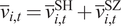
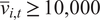
Under both regimes, eligibility is determined mechanically from preexisting holdings. If investor
$ i $
 wants to participate on day
$ t $
wants to participate on day
$ t $
 , the system computes the average value of her end-of-day stock holdings across Shanghai (SH) and Shenzhen (SZ) exchanges between
$ t-22 $
, the system computes the average value of her end-of-day stock holdings across Shanghai (SH) and Shenzhen (SZ) exchanges between
$ t-22 $
 and
$ t-2 $
and
$ t-2 $
 :
$ {\overline{v}}_{i,t}={\overline{v}}_{i,t}^{\mathrm{SH}}+{\overline{v}}_{i,t}^{\mathrm{SZ}} $
:
$ {\overline{v}}_{i,t}={\overline{v}}_{i,t}^{\mathrm{SH}}+{\overline{v}}_{i,t}^{\mathrm{SZ}} $
 . Participation requires
$ {\overline{v}}_{i,t}\ge \mathrm{10,000} $
. Participation requires
$ {\overline{v}}_{i,t}\ge \mathrm{10,000} $
 CNY. The number of lottery tickets is proportional to holdings and differs across exchanges: for SH IPOs, each ticket corresponds to 1,000 shares and each 10,000 CNY of
$ {\overline{v}}_{i,t}^{\mathrm{SH}} $
CNY. The number of lottery tickets is proportional to holdings and differs across exchanges: for SH IPOs, each ticket corresponds to 1,000 shares and each 10,000 CNY of
$ {\overline{v}}_{i,t}^{\mathrm{SH}} $
 grants one ticket; for SZ IPOs, each ticket corresponds to 500 shares and each 5,000 CNY of
$ {\overline{v}}_{i,t}^{\mathrm{SZ}} $
grants one ticket; for SZ IPOs, each ticket corresponds to 500 shares and each 5,000 CNY of
$ {\overline{v}}_{i,t}^{\mathrm{SZ}} $
 grants one ticket. Eligibility is additive across multiple IPOs on the same day. Lottery outcomes are recorded at the ticket level.
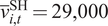
As a numerical example, suppose an investor holds
$ {\overline{v}}_{i,t}^{\mathrm{SH}}=\mathrm{29,000} $
 CNY and
$ {\overline{v}}_{i,t}^{\mathrm{SZ}}=\mathrm{8,500} $
CNY and
$ {\overline{v}}_{i,t}^{\mathrm{SZ}}=\mathrm{8,500} $
 CNY on average between
$ t-22 $
CNY on average between
$ t-22 $
 and
$ t-2 $
and
$ t-2 $
 . On day
$ t $
. On day
$ t $
 , two SH IPOs (firms
$ A $
, two SH IPOs (firms
$ A $
 and
$ B $
and
$ B $
 ) and one SZ IPO (firm
$ C $
) and one SZ IPO (firm
$ C $
 ) are open for application with IPO prices
$ {p}_{t,A}^{\mathrm{SH}}=2 $
) are open for application with IPO prices
$ {p}_{t,A}^{\mathrm{SH}}=2 $
 ,
$ {p}_{t,B}^{\mathrm{SH}}=1 $
,
$ {p}_{t,B}^{\mathrm{SH}}=1 $
 , and
$ {p}_{t,C}^{\mathrm{SZ}}=3 $
, and
$ {p}_{t,C}^{\mathrm{SZ}}=3 $
 . The investor can apply for 2,000 shares of each SH IPO and 500 shares of the SZ IPO. The maximum application value is, therefore,
$ {p}_{t,A}^{\mathrm{SH}}\times \mathrm{2,000}+{p}_{t,B}^{\mathrm{SH}}\times \mathrm{2,000}+{p}_{t,C}^{\mathrm{SZ}}\times 500=\mathrm{7,500} $
. The investor can apply for 2,000 shares of each SH IPO and 500 shares of the SZ IPO. The maximum application value is, therefore,
$ {p}_{t,A}^{\mathrm{SH}}\times \mathrm{2,000}+{p}_{t,B}^{\mathrm{SH}}\times \mathrm{2,000}+{p}_{t,C}^{\mathrm{SZ}}\times 500=\mathrm{7,500} $
 CNY. Suppose she applies for the maximum and wins one SH ticket of firm
$ B $
CNY. Suppose she applies for the maximum and wins one SH ticket of firm
$ B $
 only. Under the old regime, she submits 7,500 CNY on day
$ t $
only. Under the old regime, she submits 7,500 CNY on day
$ t $
 and receives a refund of 6,500 CNY on day
$ t+2 $
and receives a refund of 6,500 CNY on day
$ t+2 $
 . Under the new regime, she submits no cash on day
$ t $
. Under the new regime, she submits no cash on day
$ t $
 ; on day
$ t+2 $
; on day
$ t+2 $
 , she pays 1,000 CNY for the shares won.
We focus on the period between June 17, 2014, and Dec. 31, 2016, for two reasons. First, the investor-side reform occurred during this window, generating policy-driven variation. Second, the IPO PE ratio cap was strictly enforced (Figure 5), generating systematic underpricing. As a result, participating in IPO lotteries was highly attractive, supporting the identifying assumptions outlined in Section IV.B.
Figure 7 illustrates the degree of underpricing. It is noteworthy that 100% of IPO stocks in this period hit the daily upper return limits of 44% and 10% on the first and second trading days, respectively, and almost all continued hitting the 10% limit for the next several days.Footnote 14 Winning an IPO lottery was, therefore, widely perceived as a near-sure gain realized within days.
Figure 7 plots the distribution of daily returns of IPO stocks in their first 9 trading days. The sample includes 539 IPO stocks between June 17, 2014, and Dec. 31, 2016. Daily returns are capped at 44% (−44%) on the first trading day and 10% (−10%) thereafter. The limiting values at −10%, 10%, and 44% are labeled on the
$ x $
 -axis.

FIGURE 7 Long description
The nine panels are titled Day 1 through Day 9. Each panel shares a common Y-axis labeled Percentage ranging from 0 percent to 100 percent and an X-axis labeled Return with specific markers at minus 10 percent, 10 percent, and 44 percent.
* Day 1: A single vertical blue bar reaches 100 percent at the 44 percent return mark.
* Day 2: A single vertical blue bar reaches 100 percent at the 10 percent return mark.
* Day 3: A single vertical blue bar reaches 100 percent at the 10 percent return mark.
* Day 4: A single vertical blue bar reaches 100 percent at the 10 percent return mark.
* Day 5: A single vertical blue bar reaches nearly 100 percent at the 10 percent return mark, with a negligible trace near minus 10 percent.
* Day 6: The bar at 10 percent return is slightly below 100 percent, with a small cluster of bars appearing near minus 10 percent.
* Day 7: The bar at 10 percent return drops to approximately 90 percent, while the frequency of returns near minus 10 percent increases slightly.
* Day 8: The bar at 10 percent return is at approximately 85 percent, with a more visible distribution of bars between minus 10 percent and 0 percent.
* Day 9: The bar at 10 percent return is at approximately 80 percent, with the highest concentration of bars in the negative return zone compared to previous days.
Table 6 provides additional context. Total application value was 248 times the actual needed value on average under the old regime and 3,319 times under the new regime. Under both regimes, IPO stocks hit the upper limit for over 10 consecutive trading days on average. There were about 15–20 IPO stocks per month in this period, indicating that IPO events were frequent rather than exceptional.

TABLE 6 Long description
Panel A. Old Regime (June 17, 2014, to Dec. 31, 2015) with 297 observations:
* Mean: App. Account 1,204.39; Overbuy 248.12; Winning Odds 0.53; Up Limit Days 10.65; I P Os Per Month 15.63.
* Std. Dev.: App. Account 729.87; Overbuy 134.78; Winning Odds 0.30; Up Limit Days 5.43; I P Os Per Month 14.82.
* Min: App. Account 381.62; Overbuy 55.64; Winning Odds 0.12; Up Limit Days 1.00; I P Os Per Month 0.00.
* Median: App. Account 984.18; Overbuy 216.00; Winning Odds 0.46; Up Limit Days 10.00; I P Os Per Month 11.00.
* Max: App. Account 7,301.31; Overbuy 808.78; Winning Odds 1.80; Up Limit Days 29.00; I P Os Per Month 48.00.
Panel B. New Regime (Jan. 1, 2016, to Dec. 31, 2016) with 242 observations:
* Mean: App. Account 11,234.08; Overbuy 3,318.66; Winning Odds 0.05; Up Limit Days 12.69; I P Os per Month 20.17.
* Std. Dev.: App. Account 2,122.57; Overbuy 1,772.70; Winning Odds 0.05; Up Limit Days 4.84; I P Os per Month 13.10.
* Min: App. Account 6,698.16; Overbuy 213.99; Winning Odds 0.01; Up Limit Days 2.00; I P Os per Month 4.00.
* Median: App. Account 11,365.64; Overbuy 2,963.95; Winning Odds 0.03; Up Limit Days 12.50; I P Os per Month 15.00.
* Max: App. Account 15,262.79; Overbuy 8,568.76; Winning Odds 0.47; Up Limit Days 29.00; I P Os per Month 49.00.
B. Identifying Assumptions and Hypothesis
The institutional setting implies two identifying assumptions. The first delivers a testable prediction under the temperature framework. The second clarifies why the variation we exploit is plausibly orthogonal to contemporaneous stock-choice shocks.
Assumption I1. Refunded IPO cash under the old regime is cold cash.
This assumption maps directly into the temperature framework in Section II. Submitting cash for IPO participation under the old regime is a deliberate reallocation of brokerage cash into a segregated IPO cash pool. The pool is administratively frozen for a fixed 2-day window and, except for any payment for allocated shares, the deposit is refunded mechanically. In the language of the framework, cash placed into a stable container inherits the container’s temperature (Assumption T2). The key institutional feature is the high predictability of both the holding period and the redemption of principal.
A natural question is whether IPO participation resembles purchasing a lottery ticket and therefore “heats up” the cash. Although intuitive, the analogy does not fully apply in this setting. Buying a lottery ticket entails a high probability of permanently losing the ticket price. By contrast, under the old Chinese IPO regime, applicants almost surely received their deposit back because winning odds were low, and principal was not exposed to price risk while frozen. For winners, only a small share of the deposit was converted into IPO shares; during our sample period, underpricing induced by the PE cap and binding daily price limits made short-horizon IPO gains highly predictable (Figure 7). Investors participated routinely and understood the process as temporarily parking cash in an authority-guarded escrow-like account in exchange for a small chance of obtaining a near-sure gain. These features make the IPO cash pool a plausible cold container and the subsequent refund a plausible cold-cash shock. However, we do not observe investors’ perceptions of refunded IPO cash directly, so Assumption I1 should be understood as a maintained assumption grounded in the institutional features of the setting.
Assumption I2. The extent of IPO-lottery participation is not driven by an investor’s stock choices on the IPO-result announcement day or by shocks to unobserved investor characteristics that affect those stock choices.
For identification, it suffices that transitory shocks to unobserved investor characteristics around IPO events are not systematically related to both ex ante participation and ex post stock choices, conditional on controls. The exceptional attractiveness and routine nature of IPO events imply that, under the old regime, deposit submission is primarily motivated by participation in the IPO lottery rather than by plans to buy particular secondary market stocks on the announcement day, mitigating reverse-causality concerns. Moreover, participation is governed by eligibility and take-up. In the aforementioned numerical example, eligibility is the maximum amount the investor can apply for (7,500 CNY). Under the old regime, take-up is directly observed, which may vary because participation ties up liquidity for 2 days. Under the new regime, participation is essentially costless, so full take-up by eligible investors is a natural benchmark: no cash is tied up ex ante, participation rises sharply (Table 6), and winners can forgo allocation without penalty. Any occasional nonparticipation by eligible investors under the new regime would therefore overstate virtual refunds and understate the magnitudes of
$ {\beta}_1 $
 and
$ {\beta}_2 $
and
$ {\beta}_2 $
 in equation (5), implying that our estimates are conservative.
These assumptions lead to a testable prediction.
Hypothesis. Holding fixed the fraction of (actual or virtual) IPO refund in total available cash, investors under the old regime—relative to themselves under the new regime—select stocks more cautiously on IPO-result announcement days.
The hypothesis compares the two regimes at a common “refund intensity.” Consider scenario A under the old regime: an investor has 10,000 CNY available on the result day, of which 7,500 CNY arrives as an actual refund. Consider scenario B under the new regime: a comparable investor has the same 10,000 CNY available and learns that her 7,500 CNY application was unsuccessful, generating a “virtual” refund share of 75%. The difference is that in scenario A, the funds passed through the IPO cash pool and therefore underwent a cooling treatment, whereas in scenario B, they did not. Systematic differences in stock choices between the two scenarios at each refund-share level therefore trace back to the cooling treatment.
To test the hypothesis, we estimate the subsequent DiD regression:

where
$ {y}_{i,j,t} $
 is a characteristic of stock
$ j $
is a characteristic of stock
$ j $
 purchased by investor
$ i $
purchased by investor
$ i $
 on an IPO-result announcement day
$ t $
on an IPO-result announcement day
$ t $
 ;
$ {\mathrm{Refund}}_{i,t} $
;
$ {\mathrm{Refund}}_{i,t} $
 is the IPO refund amount scaled by total available cash;
$ {\mathrm{Regime}}_t $
is the IPO refund amount scaled by total available cash;
$ {\mathrm{Regime}}_t $
 equals 1 under the old regime; and
$ {controls}_{i,t} $
equals 1 under the old regime; and
$ {controls}_{i,t} $
 includes an IPO-winning indicator and the fractions of other cash sources (
$ {\mathrm{TransferIn}}_{i,t} $
includes an IPO-winning indicator and the fractions of other cash sources (
$ {\mathrm{TransferIn}}_{i,t} $
 ,
$ {\mathrm{OtherSell}}_{i,t} $
,
$ {\mathrm{OtherSell}}_{i,t} $
 ,
$ {\mathrm{Div}}_{i,t} $
,
$ {\mathrm{Div}}_{i,t} $
 , and
$ {B}_{i,t-1}^{\mathrm{end}} $
, and
$ {B}_{i,t-1}^{\mathrm{end}} $
 ), as well as the same set of controls used in regression in equation (4). Account fixed effects (
$ {\lambda}_i $
), as well as the same set of controls used in regression in equation (4). Account fixed effects (
$ {\lambda}_i $
 ) and day fixed effects (
$ {\lambda}_t $
) and day fixed effects (
$ {\lambda}_t $
 ) are included;
$ {\mathrm{Regime}}_t $
) are included;
$ {\mathrm{Regime}}_t $
 is omitted due to collinearity with day fixed effects.
IPO shares obtained in a lottery are not tradable until 1–2 weeks after the result announcement. Accordingly, stock
$ j $
 in equation (5) is a stock purchased in the secondary market, not the IPO stock.
The key parameter is
$ {\beta}_1 $
 , which captures the incremental effect of an actual (cooled) refund under the old regime relative to a virtual (uncooled) refund under the new regime at the same refund-share level. The hypothesis implies
$ {\beta}_1<0 $
, which captures the incremental effect of an actual (cooled) refund under the old regime relative to a virtual (uncooled) refund under the new regime at the same refund-share level. The hypothesis implies
$ {\beta}_1<0 $
 (
$ {\beta}_1>0 $
(
$ {\beta}_1>0 $
 ) for characteristics that are negatively (positively) related to cautiousness.
C. Results and Discussion
In our data set, we observe IPO deposits and refunds directly under the old regime. Under the new regime, by design, there is no corresponding cash flow. To construct
$ {\mathrm{Refund}}_{i,t} $
 on postreform days, we assume that eligible investors participate to the full extent under the new regime. Specifically, we use the holdings-implied maximum eligible amount as the (unobserved) application amount for each investor–IPO pair and combine it with lottery winning records, inferred from subsequent holdings, to compute a “virtual” IPO refund.
We restrict attention to secondary market stock purchases on IPO-result announcement days so that the refund shock is not confounded by delays. To mitigate concerns about multiple accounts, we drop accounts with any over-application record—cases in which observed IPO deposits under the old regime, or win amounts under either regime, exceed the holdings-implied maximum application amount. Under the new regime, we truncate the virtual refund share to lie in
$ \left[0,1\right] $
 to ensure comparability.Footnote
15 The final sample consists of 227,018 purchase observations from 9,241 investors across 238 IPO-result announcement days.
to ensure comparability.Footnote
15 The final sample consists of 227,018 purchase observations from 9,241 investors across 238 IPO-result announcement days.
Table 7 reports DiD estimates for the same nine stock characteristics examined in the algorithm-based analysis. Receiving an actual (cooled) IPO refund under the old regime leads investors to buy stocks that are safer (column 1), exhibit lower valuation and weaker recent run-ups (columns 2–3), have better long-run subsequent performance (column 5), are less attention-grabbing (columns 6–7), are more likely to be index-members (column 8), and are held longer (column 9).

TABLE 7 Long description
The table consists of nine numbered columns. The headers are grouped as follows: Column 1 is Risk (Realized Vlt.); Columns 2 and 3 are Price (M-B and M O M); Columns 4 and 5 are Performance (Short and Long); Columns 6 and 7 are Attention (Abn. Trd. and Prev. Ret.); Columns 8 and 9 are Others (Index and Horizon).
Row 1: Refund sub i,t times Regime sub t. The coefficients are:
- Column 1: -0.076*** (t-stat -2.64)
- Column 2: -26.798** (t-stat -2.26)
- Column 3: -1.544*** (t-stat -3.18)
- Column 4: 0.217 (t-stat 0.88)
- Column 5: 2.405** (t-stat 2.46)
- Column 6: -11.226*** (t-stat -2.69)
- Column 7: -0.264*** (t-stat -3.26)
- Column 8: 3.259*** (t-stat 2.98)
- Column 9: 10.259*** (t-stat 4.60)
Row 2: Refund sub i,t. The coefficients are:
- Column 1: 0.080*** (t-stat 3.99)
- Column 2: 16.439* (t-stat 1.86)
- Column 3: 0.830*** (t-stat 2.95)
- Column 4: -0.151 (t-stat -0.85)
- Column 5: -2.184*** (t-stat -2.97)
- Column 6: 9.299*** (t-stat 3.51)
- Column 7: 0.141*** (t-stat 2.67)
- Column 8: -1.759** (t-stat -2.42)
- Column 9: -3.898*** (t-stat -4.98)
Bottom rows indicate that Controls, Account F E, and Day F E are all included (Y) for all columns. Adjusted R super 2 values range from 0.1170 to 0.5340. The number of observations ranges from 211,969 to 227,018.
Overall, the DiD results indicate that investors deploy colder cash more cautiously than hotter cash, consistent with a causal cash-temperature effect. In economic terms, consider an investor for whom the refund accounts for all available cash on the purchase day (i.e., a refund share of 100%). Relative to a virtual refund of the same share under the new regime, an actual cooled refund under the old regime shifts the characteristics of purchased stocks by roughly 2.3 cross-sectional percentiles in realized volatility and 2.8 percentiles in momentum (Table A20 in the Supplementary Material), with similarly meaningful effects on future performance and attention-grabbing characteristics.
The estimates are robust to alternative specifications, including different horizons in characteristic construction and nonlinear transformations of dependent variables.Footnote 16
Instrumental-Variable Evidence
A remaining concern is that the algorithm-based temperature measure
$ {\theta}_{i,t} $
 may be endogenous at the investor-day level. The IPO reform provides a clean source of exogenous variation in temperature: holding fixed the refund share
$ {\mathrm{Refund}}_{i,t} $
may be endogenous at the investor-day level. The IPO reform provides a clean source of exogenous variation in temperature: holding fixed the refund share
$ {\mathrm{Refund}}_{i,t} $
 , only under the old regime does the refund pass through the frozen IPO cash pool and undergo the cooling treatment. We, therefore, instrument
$ {\theta}_{i,t} $
, only under the old regime does the refund pass through the frozen IPO cash pool and undergo the cooling treatment. We, therefore, instrument
$ {\theta}_{i,t} $
 with
$ {\mathrm{Refund}}_{i,t}\times {\mathrm{Regime}}_t $
with
$ {\mathrm{Refund}}_{i,t}\times {\mathrm{Regime}}_t $
 and estimate a 2SLS version of the baseline regressions.
Table 8 reports the 2SLS estimates. Panel A shows a strong first stage: the excluded instrument
$ {\mathrm{Refund}}_{i,t}\times {\mathrm{Regime}}_t $
 is highly significant, and the Kleibergen–Paap rk Wald
$ F $
is highly significant, and the Kleibergen–Paap rk Wald
$ F $
 statistic is 28,434, indicating that weak-instrument concerns are immaterial. The negative first-stage coefficient implies that, for a given refund share, cash is materially colder under the old regime than under the new regime, consistent with the cooling channel implied by Assumption I1.

TABLE 8 Long description
Panel A. First Stage. The dependent variable is theta sub i comma t. The excluded instrument is Refund sub i comma t times Regime sub t with a coefficient of minus 1.029 and a t-statistic of minus 168.62. The Refund sub i comma t coefficient is 0.061 with a t-statistic of 16.35. Controls, Account F E, and Day F E are all included. Number of observations is 227,014. Kleibergen-Paap r k Wald F is 28,434.
Panel B. Second Stage. Reports estimates of outcome variables on the instrumented theta sub i comma t I V.
Column 1: Risk (Realized Vlt.) is 0.074 with t-statistic 2.64.
Column 2: Price (M-B) is 26.055 with t-statistic 2.26.
Column 3: Price (MOM) is 1.500 with t-statistic 3.16.
Column 4: Performance (Short) is minus 0.211 with t-statistic minus 0.88.
Column 5: Performance (Long) is minus 2.337 with t-statistic minus 2.46.
Column 6: Attention (Abn. Trd.) is 10.893 with t-statistic 2.69.
Column 7: Attention (Prev. Ret.) is 0.256 with t-statistic 3.24.
Column 8: Others (Index) is minus 3.166 with t-statistic minus 2.97.
Column 9: Others (Horizon) is minus 9.967 with t-statistic minus 4.63.
All columns include Controls, Account F E, and Day F E. Observation counts range from 211,965 to 227,014.
Panel B shows that second-stage estimates line up with the temperature framework. Hotter cash (a higher instrumented
$ {\theta}_{i,t} $
 ) leads investors to buy stocks with higher realized volatility (column 1), higher valuation and stronger momentum (columns 2–3), worse long-run subsequent performance (column 5), and more attention-grabbing characteristics (columns 6–7). Hotter cash is also associated with a lower propensity to buy index-member stocks and shorter holding horizons (columns 8–9). Short-term subsequent performance is not statistically distinguishable from zero in this design (column 4). Overall, the IV results complement the DiD evidence and provide a direct quasi-experimental link from the reform-induced cooling variation to the algorithm-based temperature measure.
Supplementary Material Table A21 reports two additional sample restrictions. Panel A restricts attention to refund-dominant observations—cases in which the refund share is either very small or very large—so that IPO refunds are either effectively irrelevant or close to the sole driver of available cash on that day. Panel B excludes observations consistent with immediate refund-management strategies, in which the refund is transferred out on the same day under the old regime, making it unlikely to be used for secondary market purchases. Across both panels, second-stage estimates remain qualitatively unchanged and economically comparable, and first-stage
$ F $
 statistics remain large.
V. An Experiment
This section presents a preregistered online experiment that randomly assigns cash source and elicits risk-taking. The objective is to isolate the underlying preference channel in a controlled environment rather than to reproduce all features of the field setting.
A. Experimental Design
The preregistered online experiment was conducted on Oct. 18, 2023.Footnote 17 We recruited 405 participants from Prolific who passed the attention check and submitted complete responses. Prolific is a platform that facilitates the recruitment of diverse survey and experiment participants and is widely used in finance and economics (Bergman, Chinco, Hartzmark, and Sussman (Reference Bergman, Chinco, Hartzmark and Sussman2020)). We imposed standard eligibility criteria (U.S. residence, English proficiency, and a 100% previous approval rate). The median duration of the experiment was 9 minutes.
At the beginning of the experiment, each participant was endowed with both a savings account and a brokerage account, each containing 100 Lira (a hypothetical currency convertible to USD at a 200:1 ratio). For the first 9 periods, participants observed the evolution of these accounts without making decisions. The savings account accrued a risk-free return, while the brokerage account was invested in a volatile stock whose price fluctuated each period. A mandatory 5-second pause between periods encouraged attention to account changes.
The key decision occurred in period 10. Participants were informed that the money in both accounts was now available for use. The savings-account balance (109.37 Lira) and the brokerage-account balance (108.66 Lira) were fixed across subjects and intentionally close to rule out wealth effects. Participants were then randomly assigned to one of two treatments: a savings-account treatment, in which they used the savings-account balance to purchase a risky stock, and a brokerage-account treatment, in which they used the brokerage-account balance.
Two stocks,
$ M $
 and
$ N $
and
$ N $
 , were available in period 10. Both had a price of 100 Lira per share and a binary next-period price outcome with equal probabilities. Specifically, the next-period price of stock
$ M $
, were available in period 10. Both had a price of 100 Lira per share and a binary next-period price outcome with equal probabilities. Specifically, the next-period price of stock
$ M $
 was
$ {p}_{M,L} $
was
$ {p}_{M,L} $
 or
$ {p}_{M,H} $
or
$ {p}_{M,H} $
 with probability 0.5 each; similarly, stock
$ N $
with probability 0.5 each; similarly, stock
$ N $
 ’s next-period price was
$ {p}_{N,L} $
’s next-period price was
$ {p}_{N,L} $
 or
$ {p}_{N,H} $
or
$ {p}_{N,H} $
 with probability 0.5 each. To probe mechanisms, we considered two payoff scenarios: a loss-likely scenario with
$ \left(\mathrm{90,110,50,150}\right) $
with probability 0.5 each. To probe mechanisms, we considered two payoff scenarios: a loss-likely scenario with
$ \left(\mathrm{90,110,50,150}\right) $
 for
$ \left({p}_{M,L},{p}_{M,H},{p}_{N,L},{p}_{N,H}\right) $
for
$ \left({p}_{M,L},{p}_{M,H},{p}_{N,L},{p}_{N,H}\right) $
 and a loss-unlikely scenario with
$ \left(\mathrm{140,160,100,200}\right) $
and a loss-unlikely scenario with
$ \left(\mathrm{140,160,100,200}\right) $
 . In both scenarios, stocks
$ M $
. In both scenarios, stocks
$ M $
 and
$ N $
and
$ N $
 have the same expected return but different risk. The experiment, therefore, has four groups—each combining one treatment with one scenario—and targeted a sample size of about 100 per group.
After participants made an unalterable stock selection in period 10 but before observing the realized outcome, we elicited three postinvestment evaluations in randomized order. Participants rated, separately for each account, i) risk tolerance, ii) disutility from a hypothetical loss of 50 Lira, and iii) utility from a hypothetical gain of 50 Lira, each on a 0–10 slider scale. See Supplementary Material Section C for detailed instructions and question wording.
This design has three advantages. First, it requires no active choice until the final period, which limits confounding influences from earlier decisions and isolates the temperature manipulation. Second, because both accounts start from and end with comparable endowments, wealth and house money effects are also mitigated. Third, contrasting loss-likely and loss-unlikely environments directly isolates whether the effect hinges on sensitivity to losses, which is central to our proposed mechanism. At the same time, the design is intentionally parsimonious. Participants make a single terminal choice, so the experiment is designed to isolate the preference channel rather than to directly test the refreshing and decay of cash labels over repeated account activity.
The naming of the two accounts is intentional. The instructions emphasized that the accounts are economically equivalent in payoff convertibility and that all funds belong to the participant. Any differential perceptions induced by account labels and observed dynamics are therefore central to the mechanism. In the language of our framework, these perceptions correspond to temperature assimilation (Assumption T2 in Section II). Differential behavior across treatments, despite clarifications of economic equivalence, therefore provides direct evidence of perceived nonfungibility.
Finally, while the field evidence spans multiple stock-characteristic dimensions, the experiment focuses primarily on risk. With a two-stock choice and a modest sample size, risk is the most direct and best-powered outcome.
B. Main Result
Figure 8 reports the fraction of participants choosing the riskier stock
$ N $
 across the four groups. Under the loss-likely scenario, the cash-temperature effect is economically sizable: participants assigned to use higher-temperature brokerage cash are more likely to select the riskier stock than those assigned to use savings cash, with the share choosing
$ N $
across the four groups. Under the loss-likely scenario, the cash-temperature effect is economically sizable: participants assigned to use higher-temperature brokerage cash are more likely to select the riskier stock than those assigned to use savings cash, with the share choosing
$ N $
 rising from 39% to 53%—a 14-percentage-point increase (about 36% relative to the savings-cash baseline). By contrast, under the loss-unlikely scenario, this between-treatment difference is absent.
Figure 8 plots the proportion of subjects who choose the riskier stock in period 10. The left pair of bars corresponds to the loss-likely scenario, and the right pair corresponds to the loss-unlikely scenario. Bars compare the brokerage-account treatment and the savings-account treatment (as indicated in the figure legend).

This pattern points naturally to loss aversion. A key implication of prospect theory (Kahneman and Tversky (Reference Kahneman and Tversky1979)) is that losses generate disproportionately large disutility relative to gains of the same magnitude. The fact that the treatment effect appears only when losses are possible suggests that cash source operates primarily through sensitivity to losses rather than through a general shift in risk appetite. This mechanism guides the modeling approach in Section VI.
We also note that the overall share choosing the riskier stock is lower in the loss-unlikely scenario.Footnote
18 One plausible interpretation is that, in this scenario, stock
$ M $
 offers a salient sure gain of 40 Lira in its worst case, which may serve as a reference point. Relative to that benchmark, choosing
$ N $
offers a salient sure gain of 40 Lira in its worst case, which may serve as a reference point. Relative to that benchmark, choosing
$ N $
 exposes the participant to the possibility of forgoing the sure gain, which may itself be perceived as a reference-point loss.
To probe perceptions directly, we elicit postinvestment evaluations for each account after the stock selection but before outcome realization. For each question, subjects rate the brokerage and savings accounts separately on a 0–10 scale. Figure 9 reports average scores and 95% confidence intervals.
Figure 9 reports average responses to three postinvestment questions, pooled across treatment groups. Graph A reports perceived risk tolerance (0: strongly prefer saving at a risk-free rate; 10: strongly prefer investing in risky assets even when large gains and losses are possible). Graph B reports disutility from a hypothetical loss of 50 Lira (0: not painful; 10: very painful). Graph C reports utility from a hypothetical gain of 50 Lira (0: not exciting; 10: very exciting). Within each panel, the left pair corresponds to the loss-likely scenario and the right pair corresponds to the loss-unlikely scenario. Bars compare evaluations of the brokerage and savings accounts (as indicated in the figure legend). Confidence intervals are 95%.

FIGURE 9 Long description
A three-panel set of bar charts. Each chart features a legend at the bottom indicating light red bars for Brokerage and dark teal bars for Savings. All charts include 95 percent confidence interval error bars.
Panel A, Risk Tolerance. The y-axis ranges from 0 to 7. In the Loss-Likely scenario, Brokerage is approximately 6.2 and Savings is approximately 2.5. In the Loss-Unlikely scenario, Brokerage is approximately 6.4 and Savings is approximately 2.6.
Panel B, Disutility from Loss. The y-axis ranges from 0 to 8. In the Loss-Likely scenario, Brokerage is approximately 5.0 and Savings is approximately 7.5. In the Loss-Unlikely scenario, Brokerage is approximately 4.8 and Savings is approximately 7.6.
Panel C, Utility from Gain. The y-axis ranges from 0 to 8. In the Loss-Likely scenario, Brokerage is approximately 7.7 and Savings is approximately 8.0. In the Loss-Unlikely scenario, Brokerage is approximately 7.5 and Savings is approximately 8.3.
Three observations emerge. First, perceived risk tolerance is substantially higher for brokerage cash than for savings cash. Second, the difference is driven primarily by the loss dimension: participants report significantly lower disutility from losses in the brokerage account than in the savings account, whereas the differential response to gains is comparatively modest. Third, because the loss-likely and loss-unlikely scenarios differ only in the final-period stock-selection task, the similarity of the three postinvestment responses across the two scenarios suggests that participants attended to the instructions and formed account-specific perceptions that are stable across payoff environments.
Taken together, the experimental evidence indicates that participants are more reluctant to take risk when funds are framed as coming from the savings account, and that this difference operates primarily through heightened sensitivity to losses. The experiment, therefore, helps isolate a plausible preference channel underlying the field patterns. Table A22 in the Supplementary Material Section D reports additional results on investor heterogeneity in the experiment.
C. Discussion and External Validity
The experiment is intentionally parsimonious: it holds the budget set fixed and varies only the account frame so that differences in choices and evaluations can be interpreted through the lens of loss sensitivity.
As a one-shot task, its strength is in isolating a mechanism rather than reproducing the full dynamic structure of the brokerage-account setting. In particular, the experiment does not directly test whether cash labels are refreshed by subsequent account activity or decay with the passage of inactive time. We view those dynamic predictions as coming primarily from the brokerage-account evidence, with the experiment providing complementary causal evidence that cash source affects risk-taking and that loss sensitivity is a plausible underlying mechanism.
As in any mechanism-focused design, the experiment abstracts from several features of real-world trading and uses modest stakes. Taken together with the quasi-experimental IPO refund shock and the brokerage-account evidence, however, the three settings strengthen inference through triangulation.
A natural extension is to bring the manipulation closer to brokerage cash flows by varying the framing of investable funds within a single account (e.g., “sell proceeds” vs. “fresh deposit”) while holding payoffs and probabilities fixed.
VI. Model
The experimental results in Section V suggest that cash temperature operates through an attenuation in the marginal evaluation of gains and losses, with the disutility from losses particularly sensitive to the cold- versus hot-cash frame. We develop a model to formalize this mechanism and derive equilibrium implications.
The model embeds a temperature-dependent sensitivity to future gains and losses: hotter cash reduces how strongly investors react to realized gains and losses, holding beliefs fixed. This mapping is disciplined by the experimental evidence, which holds payoff magnitudes and probabilities fixed while shifting perceived cash type across accounts. Other mappings are possible—for example, temperature could affect probability weighting or perceived risk/ambiguity—but we focus on sensitivity because it aligns most directly with the observed pattern that the same hypothetical loss is perceived as more painful under cold cash.
The model delivers three central implications that mirror our empirical findings: higher temperature increases risk-taking, raises prices, and lowers expected returns. It also generates broader predictions, including the coexistence of limited market participation and overbuying, overreaction to shocks, and price fluctuations not driven by fundamentals.
Sections VI.A–VI.C present a myopic version of the model to highlight the key mechanism and its predictions. Section VI.D extends the framework to a dynamic setting and shows how temperature smoothing emerges once cash temperature is endogenized. Section VI.E briefly discusses potential extensions to multiasset environments.
A. Setup
Consider an infinite-horizon economy in discrete time with a continuum of investors of unit mass. In each period
$ t $
 , there is a one-period risky asset in unit supply with next-period payoff
$ {d}_{t+1} $
, there is a one-period risky asset in unit supply with next-period payoff
$ {d}_{t+1} $
 , where
$ {d}_{t+1}\sim \mathcal{N}\left(\mu, {\sigma}^2\right) $
, where
$ {d}_{t+1}\sim \mathcal{N}\left(\mu, {\sigma}^2\right) $
 . Assume that
$ {\left\{{d}_{t+1}\right\}}_{t\ge 0} $
. Assume that
$ {\left\{{d}_{t+1}\right\}}_{t\ge 0} $
 are IID over time, so the risky asset has the same fundamental distribution in every period. Investors can also hold idle cash with zero net return.
Each incumbent investor exits the economy with probability
$ \eta \in \left(0,1\right) $
 in every period
$ t $
in every period
$ t $
 and consumes accumulated wealth upon exit. A new cohort of investors with mass
$ \eta $
and consumes accumulated wealth upon exit. A new cohort of investors with mass
$ \eta $
 enters each period to keep the total mass equal to 1. Each entering cohort is endowed with homogeneous initial wealth
$ {w}_0 $
enters each period to keep the total mass equal to 1. Each entering cohort is endowed with homogeneous initial wealth
$ {w}_0 $
 . In period
$ t $
. In period
$ t $
 , a cohort-
$ \tau $
, a cohort-
$ \tau $
 investor who remains in the economy has wealth
$ {w}_{\tau, t} $
investor who remains in the economy has wealth
$ {w}_{\tau, t} $
 and cash temperature
$ {\theta}_{\tau, t} $
and cash temperature
$ {\theta}_{\tau, t} $
 , observes the risky-asset price
$ {p}_t $
, observes the risky-asset price
$ {p}_t $
 , and chooses the dollar amount
$ {a}_{\tau, t} $
, and chooses the dollar amount
$ {a}_{\tau, t} $
 invested in the risky asset (so idle cash is
$ {w}_{\tau, t}-{a}_{\tau, t} $
invested in the risky asset (so idle cash is
$ {w}_{\tau, t}-{a}_{\tau, t} $
 ). Formally, the cohort-
$ \tau $
). Formally, the cohort-
$ \tau $
 value function
$ {U}_{\tau, t}\left({w}_{\tau, t};{\theta}_{\tau, t}\right) $
value function
$ {U}_{\tau, t}\left({w}_{\tau, t};{\theta}_{\tau, t}\right) $
 is defined by


where

and

In equation (6), the weight
$ {\left(1-\eta \right)}^{t^{'}-t}\eta $
 is the probability that the investor exits in period
$ {t}^{\prime }+1 $
is the probability that the investor exits in period
$ {t}^{\prime }+1 $
 conditional on being present in period
$ t $
conditional on being present in period
$ t $
 . The first two terms capture mean–variance preferences over exit wealth, where
$ \gamma $
. The first two terms capture mean–variance preferences over exit wealth, where
$ \gamma $
 measures risk aversion. The third term adds narrow-framed, period-by-period evaluation of gains and losses as in prospect theory. We adopt a linear (kinked) prospect-theory value function in equation (8), which preserves narrow framing and loss aversion while keeping the analysis tractable. Linear formulations have been used in related settings, including Barberis, Huang, and Santos (Reference Barberis, Huang and Santos2001) and Barberis and Huang (Reference Barberis and Huang2001). Prospect-theory preferences have been successful in capturing investor behavior under uncertainty (Barberis and Huang (Reference Barberis and Huang2001), Barberis et al. (Reference Barberis, Huang and Santos2001), Barberis and Xiong (Reference Barberis and Xiong2009), and Barberis, Jin, and Wang (Reference Barberis, Jin and Wang2021)). The reference point embedded in equation (8) is the status quo (the purchase price). We adopt this baseline to highlight the temperature–sensitivity channel.
The novelty lies in the mapping
$ f\left({\theta}_{\tau, t}\right) $
 from cash temperature to the sensitivity with which the cohort evaluates future gains and losses. The negative derivative of
$ f\left(\cdot \right) $
from cash temperature to the sensitivity with which the cohort evaluates future gains and losses. The negative derivative of
$ f\left(\cdot \right) $
 implies that higher temperature reduces sensitivity. Intuitively, the same one-dollar loss is less painful (and the same one-dollar gain is less exciting) when an investor uses hotter cash.
This assumption is consistent with several related theories. First, it can be motivated by prospective accounting and decoupling (Prelec and Loewenstein (Reference Prelec and Loewenstein1998)): investors may “pay” a mental cost when converting cold cash into gambling cash and subsequently react less to ongoing fluctuations. Second, it is consistent with expectation-based reference dependence (Kőszegi and Rabin (Reference Kőszegi and Rabin2006)): when cash originates from an unstable container, expectations of stability are lower, so realized gains and losses are less surprising and elicit weaker marginal reactions.
As defined in equation (9), each entering cohort starts with
$ {\theta}_{\tau, \tau }=0 $
 , implying
$ f(0)=1 $
, implying
$ f(0)=1 $
 . New investors have not yet generated transaction-return cash, so their funds are purely cold. From period
$ t=\tau +1 $
. New investors have not yet generated transaction-return cash, so their funds are purely cold. From period
$ t=\tau +1 $
 onward, the cohort receives risky-asset payoffs, which mechanically raise temperature and lower sensitivity. This temperature disparity between new and seasoned cohorts is central for the model’s predictions.
The mapping
$ f\left(\cdot \right) $
 in equation (9) is nonlinear. A linear alternative such as
$ 1-\theta $
in equation (9) is nonlinear. A linear alternative such as
$ 1-\theta $
 is feasible, but the chosen functional form has two useful properties: it transitions from concave to convex around
$ \theta =0.5 $
is feasible, but the chosen functional form has two useful properties: it transitions from concave to convex around
$ \theta =0.5 $
 and becomes relatively flat near
$ \theta =1 $
and becomes relatively flat near
$ \theta =1 $
 . Sensitivity, therefore, drops quickly at low temperature and changes little once temperature is high. Figure 10 illustrates these properties.
Figure 10 plots
$ f\left(\theta \right) $
 from equation (9) (solid) and the linear benchmark
$ 1-\theta $
from equation (9) (solid) and the linear benchmark
$ 1-\theta $
 (dashed). The function
$ f\left(\theta \right) $
(dashed). The function
$ f\left(\theta \right) $
 is concave for
$ \theta \in \left(\mathrm{0,0.5}\right) $
is concave for
$ \theta \in \left(\mathrm{0,0.5}\right) $
 and convex for
$ \theta \in \left(\mathrm{0.5,1}\right) $
and convex for
$ \theta \in \left(\mathrm{0.5,1}\right) $
 .
.

The model is not the first to introduce history dependence into prospect-theory preferences. In Barberis et al. (Reference Barberis, Huang and Santos2001), the loss-aversion parameter
$ \lambda $
 depends on prior losses. Our approach differs in two ways. First, the state variable is cash composition (temperature) rather than the history of gains and losses. Second, the sensitivity adjustment is symmetric for gains and losses: hotter cash attenuates both, whereas many history-dependent formulations focus primarily on losses. For example, Barberis et al. (Reference Barberis, Huang and Santos2001) allow history dependence primarily through losses; in our model, the sensitivity adjustment is symmetric for gains and losses. Empirically, history dependence through funding origins remains robust even after controlling flexibly for gain/loss states, motivating the temperature-based channel.
Before solving the model, we show that the maximization problem in equations (6) and (7) can be equivalently rewritten as a myopic problem when investors treat cash temperature as an exogenous state variable. We derive the main implications under this benchmark and then relax this assumption in Section VI.D, where investors internalize the effect of current portfolio choices on future temperature.
Proposition 1. For cohort
$ \tau $
 in period
$ t $
in period
$ t $
 ,
$ \forall \tau \le t $
,
$ \forall \tau \le t $
 , the portfolio choice problem in equations (6) and (7) is equivalent to


Proof. See Appendix B1 in the Supplementary Material.▪
The intuition behind Proposition 1 is straightforward. In equation (6),
$ {\theta}_{\tau, t} $
 is the only state variable, but under the myopic assumption, investors do not anticipate how current choices affect future temperature. Consequently, cohort
$ \tau $
is the only state variable, but under the myopic assumption, investors do not anticipate how current choices affect future temperature. Consequently, cohort
$ \tau $
 in period
$ t $
in period
$ t $
 evaluates future gains and losses using
$ f\left({\theta}_{\tau, t}\right) $
evaluates future gains and losses using
$ f\left({\theta}_{\tau, t}\right) $
 and treats subsequent temperature changes as unexpected shocks. Without a commitment device, investors re-optimize each period, yielding myopic portfolio choices.
B. Equilibrium
We begin by simplifying the objective function in equation (10). The linearity of the prospect-theory value function in equation (8) allows us to rewrite
$ {\unicode{x1D53C}}_t\left[v\left(\Delta {w}_{\tau, t+1}\right)\right] $
 as a linear function of
$ {a}_{\tau, t} $
as a linear function of
$ {a}_{\tau, t} $
 .
.
Lemma 1. The prospect theory term in equation (10) is a linear function of
$ {a}_{\tau, t} $
 , that is,

For
$ {a}_{\tau, t}>0 $
 ,
$ g\left({p}_t\right) $
,
$ g\left({p}_t\right) $
 is given by

where
$ \Phi \left(\cdot \right) $
 and
$ \phi \left(\cdot \right) $
and
$ \phi \left(\cdot \right) $
 are the cumulative distribution function (c.d.f.) and probability density function (p.d.f.) of the standard normal distribution, respectively.
Proof. See Appendix B2 in the Supplementary Material. ▪
Lemma 1 implies that the objective function in equation (10) is quadratic in
$ {a}_{\tau, t} $
 , yielding a closed-form optimal portfolio choice.
Proposition 2. With no short selling and no borrowing, given the risky-asset price
$ {p}_t $
 and cash temperature
$ {\theta}_{\tau, t} $
and cash temperature
$ {\theta}_{\tau, t} $
 , cohort
$ \tau $
, cohort
$ \tau $
 ’s demand for the risky asset in period
$ t $
’s demand for the risky asset in period
$ t $
 (in dollars),
$ \forall \tau \le t $
(in dollars),
$ \forall \tau \le t $
 , is
, is

with the unconstrained demand given by

where
$ f\left({\theta}_{\tau, t}\right) $
 and
$ g\left({p}_t\right) $
and
$ g\left({p}_t\right) $
 are defined in equations (9) and (13), respectively.
Proof. See Appendix B3 in the Supplementary Material. ▪
Given Proposition 2, the equilibrium price is obtained by aggregating cohort demands and imposing market clearing. Since cohort
$ \tau $
 purchases
$ {a}_{\tau, t}/{p}_t $
purchases
$ {a}_{\tau, t}/{p}_t $
 shares and supply is one share, market clearing is equivalent to
$ {\sum}_{\tau \le t}\eta {\left(1-\eta \right)}^{t-\tau }{a}_{\tau, t}={p}_t $
shares and supply is one share, market clearing is equivalent to
$ {\sum}_{\tau \le t}\eta {\left(1-\eta \right)}^{t-\tau }{a}_{\tau, t}={p}_t $
 .
.
Definition 1.
$ {p}_t $
 is an equilibrium of the economy
$ {\left\{{U}_{\tau, t},{w}_{\tau, t},{\theta}_{\tau, t}\right\}}_{\tau \le t} $
is an equilibrium of the economy
$ {\left\{{U}_{\tau, t},{w}_{\tau, t},{\theta}_{\tau, t}\right\}}_{\tau \le t} $
 in period
$ t $
in period
$ t $
 if and only if there exist
$ {\left\{{a}_{\tau, t}\right\}}_{\tau \le t} $
if and only if there exist
$ {\left\{{a}_{\tau, t}\right\}}_{\tau \le t} $
 such that:
-
1. Utility maximization: $ {\left\{{a}_{\tau, t}\right\}}_{\tau \le t} $
are given by Proposition 2; -
2. Market clearing: $ {\left\{{a}_{\tau, t}\right\}}_{\tau \le t} $
satisfy


In the initial period, there is a single cohort with mass 1 and temperature
$ {\theta}_{0,0}=0 $
 . The equilibrium price at
$ t=0 $
. The equilibrium price at
$ t=0 $
 is characterized by the following corollary.
Corollary 1. In period
$ t=0 $
 , the equilibrium price
$ {p}_0 $
, the equilibrium price
$ {p}_0 $
 is
is

where

Proof. See Appendix B4 in the Supplementary Material. ▪
C. Numerical Results
The initial price
$ {p}_0 $
 in equation (17) is the benchmark of a traditional model without a cash-temperature channel. Starting in period 1, cohort
$ \tau =0 $
in equation (17) is the benchmark of a traditional model without a cash-temperature channel. Starting in period 1, cohort
$ \tau =0 $
 receives hot cash from its
$ t=0 $
receives hot cash from its
$ t=0 $
 investment, so
$ {\theta}_{0,1} $
investment, so
$ {\theta}_{0,1} $
 rises and the cohort becomes less sensitive to gains and losses. To illustrate implications for price and participation, we simulate the economy for 50 periods, compute the average price over these periods, and report the difference between that average and
$ {p}_0 $
rises and the cohort becomes less sensitive to gains and losses. To illustrate implications for price and participation, we simulate the economy for 50 periods, compute the average price over these periods, and report the difference between that average and
$ {p}_0 $
 (scaled by
$ {p}_0 $
(scaled by
$ {p}_0 $
 ) as a heat map in Graph A of Figure 11. We also compute, in each period, the mass of investors who optimally choose zero risky holding and report the average mass over the 50 periods in Graph B of Figure 11.
Figure 11 reports sensitivity tests for loss aversion
$ \lambda \in \left[\mathrm{1.5,3.0}\right] $
 and risk aversion
$ \gamma \in \left[\mathrm{1.0,2.5}\right] $
and risk aversion
$ \gamma \in \left[\mathrm{1.0,2.5}\right] $
 . The economy is simulated for 50 periods starting from the initial period with price
$ {p}_0 $
. The economy is simulated for 50 periods starting from the initial period with price
$ {p}_0 $
 given by Corollary 1. Other parameters are initial wealth
$ {w}_0=2 $
given by Corollary 1. Other parameters are initial wealth
$ {w}_0=2 $
 , risky-asset mean and standard deviation
$ \mu =1.012 $
, risky-asset mean and standard deviation
$ \mu =1.012 $
 and
$ \sigma =0.09 $
and
$ \sigma =0.09 $
 (monthly Shanghai Stock Exchange (SSE) Composite Index returns, January–December 2016). Graph A reports overpricing (average price over 50 periods minus
$ {p}_0 $
(monthly Shanghai Stock Exchange (SSE) Composite Index returns, January–December 2016). Graph A reports overpricing (average price over 50 periods minus
$ {p}_0 $
 , scaled by
$ {p}_0 $
, scaled by
$ {p}_0 $
 ). Graph B reports the average mass of investors who choose zero risky holding over the same horizon.

FIGURE 11 Long description
Two side-by-side heat maps. Both share a vertical Y axis labeled gamma ranging from 1.1 to 2.5 and a horizontal X axis labeled lambda ranging from 1.5 to 2.9.
Graph A, titled Overpricing, shows a gradient where the highest overpricing (yellow, approximately 1.0 percent) occurs at the top-left corner where gamma is high and lambda is low. The color transitions through green to dark blue (approximately -0.2 percent) at the bottom-right corner where gamma is low and lambda is high. A vertical color scale to the right ranges from -0.2 percent to 1.0 percent.
Graph B, titled No Participation, shows a sharp diagonal divide. The top-left region is solid yellow, indicating 0 percent non-participation. Starting from the bottom-left and moving toward the bottom-right, the color transitions through green to dark purple, indicating a steep increase in non-participation. The highest non-participation (dark purple, over 30 percent) is concentrated in the bottom-right corner where gamma is low and lambda is high. A vertical color scale to the right ranges from 0 percent to 30 percent.
The key finding is that lower
$ \gamma $
 and higher
$ \lambda $
and higher
$ \lambda $
 generate both larger price increases (overpricing) and a greater fraction of nonparticipating investors. A lower
$ \gamma $
generate both larger price increases (overpricing) and a greater fraction of nonparticipating investors. A lower
$ \gamma $
 raises
$ {p}_0^{\star } $
raises
$ {p}_0^{\star } $
 via equation (18), which increases the probability of losses and therefore makes
$ g\left({p}_0^{\star}\right) $
via equation (18), which increases the probability of losses and therefore makes
$ g\left({p}_0^{\star}\right) $
 more likely to be negative. A higher
$ \lambda $
more likely to be negative. A higher
$ \lambda $
 amplifies the penalty on losses, further reducing
$ g\left({p}_0^{\star}\right) $
amplifies the penalty on losses, further reducing
$ g\left({p}_0^{\star}\right) $
 . When
$ g\left({p}_0^{\star}\right)<0 $
. When
$ g\left({p}_0^{\star}\right)<0 $
 , the prospect-theory term discourages risky holdings. Temperature dynamics relax this penalty: when the penalty is larger to begin with, the reduction in sensitivity induced by rising temperature produces a larger increase in risky demand and prices, consistent with Graph A in Figure 11. Meanwhile, entering cohorts start with
$ \theta =0 $
, the prospect-theory term discourages risky holdings. Temperature dynamics relax this penalty: when the penalty is larger to begin with, the reduction in sensitivity induced by rising temperature produces a larger increase in risky demand and prices, consistent with Graph A in Figure 11. Meanwhile, entering cohorts start with
$ \theta =0 $
 and are therefore most sensitive; when prices are high, some entrants optimally choose not to participate, explaining Graph B in Figure 11.
Simulations starting from
$ t=0 $
 highlight the mechanism but rely on the special role of cohort
$ \tau =0 $
highlight the mechanism but rely on the special role of cohort
$ \tau =0 $
 . For the subsequent main simulations, we first characterize a deterministic steady state and initialize simulations at that steady state.
Definition 2. A deterministic steady state
$ {\left\{{\hat{U}}_{\tau, t},{\hat{w}}_{\tau, t},{\hat{\theta}}_{\tau, t}\right\}}_{\tau \le t} $
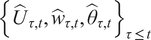 is attained in period
$ t $
is attained in period
$ t $
 if and only if:
-
1. Cohort $ \tau $
’s size is
$ \eta {\left(1-\eta \right)}^{t-\tau } $
,
$ \forall \tau \le t $
; -
2. Price, wealth distribution, and holdings distribution remain constant when the risky payoff equals its mean, that is, $ {p}_{t+1}={p}_t $
,
$ {w}_{\tau +1,t+1}={w}_{\tau, t} $
, and
$ {a}_{\tau +1,t+1}={a}_{\tau, t} $
for all
$ \tau \le t $
if
$ {d}_{t+1}=\mu $
.






Because the economy is subject to aggregate risk in every period, the steady state is defined conditional on
$ {d}_{t+1}=\mu $
 . In simulations with stochastic payoffs, the price path is relatively flat after the economy reaches this steady state. This reflects the stabilizing property of
$ f\left(\cdot \right) $
. In simulations with stochastic payoffs, the price path is relatively flat after the economy reaches this steady state. This reflects the stabilizing property of
$ f\left(\cdot \right) $
 near
$ \theta =1 $
near
$ \theta =1 $
 , which dampens the impact of small temperature fluctuations. Accordingly, the subsequent simulations emphasize temperature shocks.
We compute the deterministic steady state and then simulate the economy under different parameter values. We vary loss aversion
$ \lambda $
 (
$ 0.5{\lambda}_0 $
(
$ 0.5{\lambda}_0 $
 ,
$ {\lambda}_0 $
,
$ {\lambda}_0 $
 ,
$ 1.5{\lambda}_0 $
,
$ 1.5{\lambda}_0 $
 ), risk aversion
$ \gamma $
), risk aversion
$ \gamma $
 (1, 2, 3), replacement rate
$ \eta $
(1, 2, 3), replacement rate
$ \eta $
 (0.05, 0.1, 0.2), and temperature decay
$ \beta $
(0.05, 0.1, 0.2), and temperature decay
$ \beta $
 (1, 0.98, 0.9), taking the middle value as baseline.Footnote
19 We set
$ {\lambda}_0=2.25 $
(1, 0.98, 0.9), taking the middle value as baseline.Footnote
19 We set
$ {\lambda}_0=2.25 $
 , the value estimated for the median participant in Tversky and Kahneman (Reference Tversky and Kahneman1992). For each configuration, we impose a negative temperature shock that reduces temperature by 50% for all agents (motivated by large cold inflows such as transfers or IPO refunds) and simulate forward for 50 periods, repeating the exercise 100 times across payoff paths.Footnote
20
, the value estimated for the median participant in Tversky and Kahneman (Reference Tversky and Kahneman1992). For each configuration, we impose a negative temperature shock that reduces temperature by 50% for all agents (motivated by large cold inflows such as transfers or IPO refunds) and simulate forward for 50 periods, repeating the exercise 100 times across payoff paths.Footnote
20
Figure 12 shows that prices typically rise as aggregate temperature recovers from a negative shock (except under the lowest
$ \lambda $
 ). For sufficiently large
$ \lambda $
). For sufficiently large
$ \lambda $
 and small
$ \gamma $
and small
$ \gamma $
 , prices can overshoot and become volatile. The mechanism operates through temperature disparities across cohorts. When a negative temperature shock hits in period
$ t $
, prices can overshoot and become volatile. The mechanism operates through temperature disparities across cohorts. When a negative temperature shock hits in period
$ t $
 , existing cohorts reduce risky holdings and the price falls. The entering cohort (
$ \tau =t $
, existing cohorts reduce risky holdings and the price falls. The entering cohort (
$ \tau =t $
 ), however, starts with
$ {\theta}_{t,t}=0 $
), however, starts with
$ {\theta}_{t,t}=0 $
 and is unaffected by the shock; at the lower price, entrants are willing to absorb more risk. In period
$ t+1 $
and is unaffected by the shock; at the lower price, entrants are willing to absorb more risk. In period
$ t+1 $
 , this cohort receives payoffs from its larger position, which raises its temperature relative to the counterfactual without the shock. Before the economy transitions back to steady state, early postshock entrant cohorts therefore accumulate unusually hot cash and sustain elevated demand, generating overreaction.
Figure 12 plots equilibrium prices from simulations that start from the deterministic steady state and impose a shock that reduces cash temperature by 50% for all agents. Baseline values are
$ \lambda ={\lambda}_0 $
 (2.25),
$ \gamma =2 $
(2.25),
$ \gamma =2 $
 ,
$ \eta =0.1 $
,
$ \eta =0.1 $
 , and
$ \beta =0.98 $
, and
$ \beta =0.98 $
 . Graph A varies
$ \lambda $
. Graph A varies
$ \lambda $
 (
$ 0.5{\lambda}_0 $
(
$ 0.5{\lambda}_0 $
 and
$ 1.5{\lambda}_0 $
and
$ 1.5{\lambda}_0 $
 ); Graph B varies
$ \gamma $
); Graph B varies
$ \gamma $
 (1 and 3); Graph C varies
$ \eta $
(1 and 3); Graph C varies
$ \eta $
 (0.05 and 0.2); and Graph D varies
$ \beta $
(0.05 and 0.2); and Graph D varies
$ \beta $
 (1 and 0.9). Other parameters are
$ {w}_0=2 $
(1 and 0.9). Other parameters are
$ {w}_0=2 $
 ,
$ \mu =1.012 $
,
$ \mu =1.012 $
 , and
$ \sigma =0.09 $
, and
$ \sigma =0.09 $
 (monthly Shanghai Stock Exchange (SSE) Composite Index returns, January–December 2016). Each setting is simulated 100 times; the mean and 95% confidence interval are shown.

FIGURE 12 Long description
A four-panel line graph set. Each panel shares a common y-axis for P sub t ranging from 0.98 to 1.00 and an x-axis for time t ranging from 0 to 50.
* Top-Left (Loss Aversion): Compares lambda values. The baseline lambda sub 0 (solid grey) is stable near 0.993. 0.5 lambda sub 0 (blue dash-dot) starts high and stabilizes at 0.997. 1.5 lambda sub 0 (orange dashed) starts low and exhibits persistent oscillations between 0.983 and 0.988.
* Top-Right (Risk Aversion): Compares gamma values. Gamma equals 1 (blue dash-dot) shows high-frequency oscillations around 0.996. Gamma equals 2 (solid grey) is stable at 0.993. Gamma equals 3 (orange dashed) is stable at a lower level of 0.987.
* Bottom-Left (Replacement Rate): Compares eta values. All series converge quickly to stable horizontal lines. Eta equals 0.05 (blue dash-dot) is highest at 0.993, eta equals 0.1 (solid grey) is middle at 0.992, and eta equals 0.2 (orange dashed) is lowest at 0.991.
* Bottom-Right (Temperature Decay): Compares beta values. All three series (beta equals 1, 0.98, and 0.9) overlap almost perfectly, showing a brief initial spike before converging to a single stable line at 0.993.
The same logic also generates reversals. When the price overshoots above its steady-state level, some late postshock entrant cohorts optimally remain on the sidelines. Nonparticipation upon entry implies no participation in the next period as well because cash temperature remains at zero without realized payoffs from risky holdings. As existing cohorts gradually unwind positions as they exit, the price declines until it becomes sufficiently low that multiple sidelined cohorts re-enter simultaneously, pushing the price up again. Consistent with Figure 12, such back-and-forth adjustment is more likely when temperature disparities are stronger—that is, when
$ {\unicode{x1D53C}}_t\left[v\left(\Delta {w}_{\tau, t+1}\right)\right] $
 is larger, as implied by higher
$ \lambda $
is larger, as implied by higher
$ \lambda $
 or lower
$ \gamma $
or lower
$ \gamma $
 .
.
Figure 13 shows that aggregate temperature rises as the economy recovers from the negative shock. Parameter values that generate larger price movements also generate more pronounced temperature fluctuations, yielding positive comovement between temperature and price—consistent with the pro-cyclical patterns in Figure 3. For the nonpreference parameters, the replacement rate
$ \eta $
 is mechanically negatively related to aggregate temperature: higher turnover replaces more hot incumbents with cold entrants. The effect of the decay parameter
$ \beta $
is mechanically negatively related to aggregate temperature: higher turnover replaces more hot incumbents with cold entrants. The effect of the decay parameter
$ \beta $
 is limited because cohorts receive relatively large hot inflows through payoffs each period.
Figure 13 plots the mass-weighted average cash temperature from the simulations in Figure 12. The mean and 95% confidence interval are shown.

FIGURE 13 Long description
The figure consists of four panels, each with an x-axis representing time t from 0 to 50 and a y-axis representing theta sub t from 0.0 to 1.0.
* Top-Left Panel (Loss Aversion): Shows three lines. A blue dash-dot line for lambda equals 0.5 lambda sub 0 rises quickly and plateaus near 0.85. A solid grey line for lambda equals lambda sub 0 plateaus near 0.7. A dashed orange line for lambda equals 1.5 lambda sub 0 oscillates between 0.5 and 0.6.
* Top-Right Panel (Loss Aversion): Shows three lines. A dashed orange line for gamma equals 3 plateaus near 0.8. A solid grey line for gamma equals 2 plateaus near 0.7. A blue dash-dot line for gamma equals 1 oscillates around 0.5.
* Bottom-Left Panel (Replacement Rate): Shows three lines. A blue dash-dot line for eta equals 0.05 plateaus near 0.8. A solid grey line for eta equals 0.1 plateaus near 0.7. A dashed orange line for eta equals 0.2 plateaus near 0.6.
* Bottom-Right Panel (Temperature Decay): Shows three lines that are closely clustered. A blue dash-dot line for beta equals 1, a solid grey line for beta equals 0.98, and a dashed orange line for beta equals 0.9 all rise rapidly and plateau between 0.7 and 0.75.
Figure 14 highlights the role of disparity. Graph A shows that the entering cohort’s temperature rises from 0 toward 1 over roughly 5 periods and remains near 1 thereafter, while holdings increase as temperature rises. Graph B shows that older cohorts have similarly high temperatures and holdings, while younger cohorts have lower levels of both. The economically relevant force is, therefore, the disparity between new entrants and seasoned cohorts, rather than small differences among seasoned cohorts.
Figure 14 illustrates temperature disparity in simulations that start from the deterministic steady state and impose a 50% reduction in temperature for all agents. Parameters take baseline values:
$ \lambda ={\lambda}_0 $
 (2.25),
$ \gamma =2 $
(2.25),
$ \gamma =2 $
 ,
$ \eta =0.1 $
,
$ \eta =0.1 $
 , and
$ \beta =0.98 $
, and
$ \beta =0.98 $
 . Graph A plots holdings (top) and cash temperature (bottom) over 50 periods for the cohort entering at the shock date. Graph B plots the cross section in period 50 of holdings (top) and temperature (bottom) across cohorts. Other parameters are
$ {w}_0=2 $
. Graph A plots holdings (top) and cash temperature (bottom) over 50 periods for the cohort entering at the shock date. Graph B plots the cross section in period 50 of holdings (top) and temperature (bottom) across cohorts. Other parameters are
$ {w}_0=2 $
 ,
$ \mu =1.012 $
,
$ \mu =1.012 $
 , and
$ \sigma =0.09 $
, and
$ \sigma =0.09 $
 (monthly Shanghai Stock Exchange (SSE) Composite Index returns, January–December 2016). Each setting is simulated 100 times; the mean and 95% confidence interval are shown.

FIGURE 14 Long description
Graph A, titled Initial Cohort, contains two panels. The top panel, Holding, plots a sub 0, t against t. The blue line starts at 0.7, rises sharply until period 5, and then plateaus at 1.2 for the remainder of the 50 periods. The bottom panel, Temperature, plots theta sub 0, t against t. The dashed orange line starts at 0.0 and rises asymptotically to 1.0 by period 10, remaining flat thereafter.
Graph B, titled Cross-Section, contains two panels. The top panel, Holding, plots a sub tau, 49 against t. The blue line remains constant at 1.2 from period 0 to 45, then drops sharply to approximately 0.3 by period 50. The bottom panel, Temperature, plots theta sub tau, 49 against t. The dashed orange line remains constant at 1.0 until period 42, then drops steeply to 0.0 by period 50.
In summary, the myopic model featuring temperature disparity delivers three implications aligned with our empirical evidence: i) higher cash temperature increases risk-taking, ii) higher cash temperature raises prices, and iii) higher cash temperature lowers expected returns holding fundamentals fixed. It also generates three classic patterns: the coexistence of no participation and overbuying, overreaction to shocks, and price fluctuations not driven by fundamentals.
D. Extension to a Dynamic Setting
Proposition 1 relies on the assumption that
$ f\left({\theta}_{\tau, t}\right) $
 in equation (6) is treated as fixed across future periods when the investor solves the period-
$ t $
in equation (6) is treated as fixed across future periods when the investor solves the period-
$ t $
 problem. We now lift this restriction and consider a dynamic model in which investors internalize how current investment affects future cash temperature. We then compare the dynamic and myopic settings to highlight temperature smoothing.
Consider the subsequent dynamic variant of equations (6) and (7) for cohort
$ \tau $
 in period
$ t $
in period
$ t $
 :
:


where
$ v\left(\Delta {w}_{\tau, j+1}\right) $
 and
$ f\left({\theta}_{\tau, t}\right) $
and
$ f\left({\theta}_{\tau, t}\right) $
 are defined in equations (8) and (9), respectively. Relative to equation (6), the key difference is that sensitivity
$ f\left({\theta}_{\tau, j}\right) $
are defined in equations (8) and (9), respectively. Relative to equation (6), the key difference is that sensitivity
$ f\left({\theta}_{\tau, j}\right) $
 now evolves endogenously with the portfolio path. As a result, the first-order condition for
$ {a}_{\tau, t} $
now evolves endogenously with the portfolio path. As a result, the first-order condition for
$ {a}_{\tau, t} $
 involves
$ \partial f\left({\theta}_{\tau, j}\right)/\partial {a}_{\tau, t} $
involves
$ \partial f\left({\theta}_{\tau, j}\right)/\partial {a}_{\tau, t} $
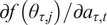 for
$ j\ge t+1 $
for
$ j\ge t+1 $
 , making the problem genuinely dynamic.Footnote
21
, making the problem genuinely dynamic.Footnote
21
The dynamic problem is challenging. We, therefore, apply a simplifying approximation that preserves the key economics. In Graph A of Figure 15, we plot
$ f\left({\theta}_{\tau, \tau +j}\right) $
 for
$ j=\mathrm{1,2,3,4} $
for
$ j=\mathrm{1,2,3,4} $
 against initial risky holding
$ {a}_{\tau, \tau } $
against initial risky holding
$ {a}_{\tau, \tau } $
 .Footnote
22 An important observation is that
.Footnote
22 An important observation is that

approximately holds over the relevant range of
$ {a}_{\tau, \tau } $
 (marked in gray), which implies that initial portfolio choice mainly affects next-period sensitivity.
Graph A in Figure 15 plots sensitivity
$ f\left({\theta}_{\tau, \tau +j}\right) $
 for
$ j=\mathrm{1,2,3,4} $
for
$ j=\mathrm{1,2,3,4} $
 against initial risky holding
$ {a}_{\tau, \tau } $
against initial risky holding
$ {a}_{\tau, \tau } $
 , where
$ f\left(\cdot \right) $
, where
$ f\left(\cdot \right) $
 is defined in equation (9). Results are based on the deterministic steady state with
$ \beta =1 $
is defined in equation (9). Results are based on the deterministic steady state with
$ \beta =1 $
 and baseline parameter values
$ \lambda ={\lambda}_0 $
and baseline parameter values
$ \lambda ={\lambda}_0 $
 (2.25),
$ \gamma =2 $
(2.25),
$ \gamma =2 $
 , and
$ \eta =0.1 $
, and
$ \eta =0.1 $
 . Initial wealth is set to
$ {w}_{\tau, \tau }=1.387 $
. Initial wealth is set to
$ {w}_{\tau, \tau }=1.387 $
 so that the model’s optimal idle-cash share matches the brokerage-cash share in the data. The gray band marks the interval
$ \left[{\underline{a}}_{\tau, \tau },{\overline{a}}_{\tau, \tau}\right] $
so that the model’s optimal idle-cash share matches the brokerage-cash share in the data. The gray band marks the interval
$ \left[{\underline{a}}_{\tau, \tau },{\overline{a}}_{\tau, \tau}\right] $
 , where
$ {\underline{a}}_{\tau, \tau }=0.884 $
, where
$ {\underline{a}}_{\tau, \tau }=0.884 $
 and
$ {\overline{a}}_{\tau, \tau }=1.176 $
and
$ {\overline{a}}_{\tau, \tau }=1.176 $
 are the minimum and maximum optimal risky holdings corresponding to temperature 0 and 1. Graph B plots the temperature-smoothing term
$ {\xi}_{\tau, \tau +1} $
are the minimum and maximum optimal risky holdings corresponding to temperature 0 and 1. Graph B plots the temperature-smoothing term
$ {\xi}_{\tau, \tau +1} $
 defined in equation (24) against
$ {a}_{\tau, \tau } $
defined in equation (24) against
$ {a}_{\tau, \tau } $
 under the same settings.

FIGURE 15 Long description
Graph A, titled Future Sensitivities, plots f(theta sub tau, tau + j) on the y-axis from 0.0 to 1.0 against a sub tau, tau on the x-axis from 0.000 to 1.387. Four lines represent j = 1, 2, 3, and 4. The j = 1 line is a solid blue curve starting at 1.0 and decreasing to 0.0 near x = 1.1. The j = 2 line is a dashed orange line starting at approximately 0.15 and reaching 0.0 by x = 0.6. The j = 3 and j = 4 lines are flat at 0.0. A vertical gray band is positioned between x = 0.884 and x = 1.176.
Graph B, titled Temperature Smoothing, plots xi sub tau, tau + j on the y-axis from -1.0 to 0.0 against a sub tau, tau on the x-axis from 0.000 to 1.387. A single solid blue line for j = 1 starts at approximately -0.7 at x = 0.0, follows an S-shaped upward curve, and plateaus at 0.0 around x = 0.9.
Motivated by this approximation, we adopt the simplifying condition

which yields results that are quantitatively close to those from the full dynamic problem.
Proposition 3 solves equations (19) and (20) under equation (22), and Proposition 4 compares optimal holding paths with and without internalizing the temperature channel. The qualitative takeaway is robust to relaxing equation (22).Footnote 23
Proposition 3. For cohort
$ \tau $
 in period
$ t $
in period
$ t $
 ,
$ \forall t\ge \tau $
,
$ \forall t\ge \tau $
 , given the deterministic steady-state price
$ \hat{p} $
, given the deterministic steady-state price
$ \hat{p} $
 of the risky asset and cash temperature
$ {\theta}_{\tau, t} $
of the risky asset and cash temperature
$ {\theta}_{\tau, t} $
 , the interior solution to problem in equations (19) and (20) with
$ \beta =1 $
, the interior solution to problem in equations (19) and (20) with
$ \beta =1 $
 and condition in equation (22) is characterized by

where the temperature smoothing term
$ {\xi}_{\tau, t}\left({\hat{a}}_{\tau, t}^{\star },{\hat{a}}_{\tau, t+1}^{\star };{\theta}_{\tau, t},{w}_{\tau, t}\right) $
 is given by

Proof. See Appendix B6 in the Supplementary Material. ▪
Relative to the myopic solution
$ {a}_{\tau, t}^{\star } $
 in equation (15), the dynamic solution in equation (23) differs only through the additional term
$ {\xi}_{\tau, t}\left(\cdot \right) $
in equation (15), the dynamic solution in equation (23) differs only through the additional term
$ {\xi}_{\tau, t}\left(\cdot \right) $
 that modifies the coefficient on the penalty term
$ g\left(\hat{p}\right) $
that modifies the coefficient on the penalty term
$ g\left(\hat{p}\right) $
 . The comparison between
$ {\hat{a}}_{\tau, t}^{\star } $
. The comparison between
$ {\hat{a}}_{\tau, t}^{\star } $
 and
$ {a}_{\tau, t}^{\star } $
and
$ {a}_{\tau, t}^{\star } $
 is, therefore, governed by the sign of
$ {\xi}_{\tau, t}\left(\cdot \right) $
is, therefore, governed by the sign of
$ {\xi}_{\tau, t}\left(\cdot \right) $
 .
.
Proposition 4. Under regularity conditions, let
$ {\left\{{\hat{a}}_{\tau, t}^{\star}\right\}}_{t=\tau}^{\infty } $
 denote the sequence implied by equation (23) and
$ {\left\{{a}_{\tau, t}^{\star}\right\}}_{t=\tau}^{\infty } $
denote the sequence implied by equation (23) and
$ {\left\{{a}_{\tau, t}^{\star}\right\}}_{t=\tau}^{\infty } $
 the sequence given by equation (15) at the deterministic steady state. Then temperature smoothing obtains:
-
1. upon entry, $ {\hat{a}}_{\tau, \tau}^{\star }>{a}_{\tau, \tau}^{\star } $
; -
2. there exists $ {t}_0>\tau $
such that
$ {\hat{a}}_{\tau, {t}_0}^{\star }<{a}_{\tau, {t}_0}^{\star } $
.


Proof. See Appendix B7 in the Supplementary Material. ▪
Graph B in Figure 15 sheds light on the mechanism. The temperature-smoothing term
$ {\xi}_{\tau, \tau +1} $
 in equation (24) is strongly negative when the entrant’s initial risky position is too small to generate enough hot cash to raise temperature in period
$ \tau +1 $
in equation (24) is strongly negative when the entrant’s initial risky position is too small to generate enough hot cash to raise temperature in period
$ \tau +1 $
 . Entrants who internalize the cash-temperature channel, therefore, have a strong incentive to invest sufficiently today to avoid remaining in a high-sensitivity (cold) state tomorrow. This force implies
$ {\hat{a}}_{\tau, \tau}^{\star }>{a}_{\tau, \tau}^{\star } $
. Entrants who internalize the cash-temperature channel, therefore, have a strong incentive to invest sufficiently today to avoid remaining in a high-sensitivity (cold) state tomorrow. This force implies
$ {\hat{a}}_{\tau, \tau}^{\star }>{a}_{\tau, \tau}^{\star } $
 when sensitivity is highest upon entry. As temperature rises and sensitivity falls, the sign reverses: in a later period
$ {t}_0 $
when sensitivity is highest upon entry. As temperature rises and sensitivity falls, the sign reverses: in a later period
$ {t}_0 $
 ,
$ {\xi}_{\tau, {t}_0}\left(\cdot \right)>0 $
,
$ {\xi}_{\tau, {t}_0}\left(\cdot \right)>0 $
 implies
$ {\hat{a}}_{\tau, {t}_0}^{\star }<{a}_{\tau, {t}_0}^{\star } $
implies
$ {\hat{a}}_{\tau, {t}_0}^{\star }<{a}_{\tau, {t}_0}^{\star } $
 , so the dynamic investor tilts toward a smaller risky position than the myopic benchmark. Anticipating how today’s choice affects tomorrow’s temperature thus smooths the time path of risky holdings, and for any initial
$ {a}_{\tau, \tau } $
, so the dynamic investor tilts toward a smaller risky position than the myopic benchmark. Anticipating how today’s choice affects tomorrow’s temperature thus smooths the time path of risky holdings, and for any initial
$ {a}_{\tau, \tau } $
 within the relevant range, temperature approaches 1 and sensitivity approaches 0 relatively quickly. The same pattern holds across parameter values (Supplementary Material Section B5).
Three insights follow. First, the myopic model predicts sharp differences between entering and existing cohorts due to temperature disparity; the dynamic model attenuates these differences because investors internalize and partially offset the cash-temperature effect. Empirically, strong responses to cold-cash injections, as we find, suggest that the effect is not fully internalized.
Second, internalizing the effect improves time consistency but does not eliminate the channel.Footnote 24 Even in the dynamic model, relative to a counterfactual economy in which temperature is always 0, investors hold more risk, prices are higher, and expected returns are lower.
Finally, the fact that understanding the mechanism does not eliminate it points to potential policy interventions. Although a one-time cold-cash injection may have little effect once the mechanism is well understood, regular cold-cash arrivals can still shape behavior. For example, if stock-sale proceeds are routinely routed first into a savings account (a cold container) rather than credited directly to brokerage cash, investors may trade more cautiously.Footnote 25
E. Discussion: A Multiasset Environment
Section VI.D shows that cash temperature is a state variable that investors may rationally internalize because today’s trades affect the composition—and hence the temperature—of tomorrow’s investable cash. The mechanism does not rely on there being only one risky asset. What matters is that, holding beliefs fixed, colder cash makes losses feel more salient and increases the marginal disutility of downside outcomes.
To see this in a standard
$ N $
 -asset environment, let
$ {x}_t\in {\mathrm{\mathbb{R}}}^N $
-asset environment, let
$ {x}_t\in {\mathrm{\mathbb{R}}}^N $
 denote the vector of new purchases (or risky positions) chosen at date
$ t $
denote the vector of new purchases (or risky positions) chosen at date
$ t $
 , with excess return vector
$ {\tilde{R}}_{t+1} $
, with excess return vector
$ {\tilde{R}}_{t+1} $
 . A parsimonious way to embed temperature is to augment a benchmark expected-utility objective with a temperature-indexed penalty for downside outcomes:

where
$ \phi \left(\cdot \right) $
 is increasing and convex on
$ {\mathrm{\mathbb{R}}}_{+} $
is increasing and convex on
$ {\mathrm{\mathbb{R}}}_{+} $
 (e.g., a prospect-theory-style loss term) and
$ \Lambda \left({\theta}_t\right) $
(e.g., a prospect-theory-style loss term) and
$ \Lambda \left({\theta}_t\right) $
 is decreasing in temperature (colder cash
$ \Rightarrow $
is decreasing in temperature (colder cash
$ \Rightarrow $
 larger
$ \Lambda $
larger
$ \Lambda $
 ). This formulation captures the preference-based channel documented in the experiment and provides a multiasset counterpart to the myopic and dynamic single-asset models: when
$ {\theta}_t $
). This formulation captures the preference-based channel documented in the experiment and provides a multiasset counterpart to the myopic and dynamic single-asset models: when
$ {\theta}_t $
 is low, investors behave as if downside payoffs carry a larger shadow cost, holding beliefs fixed.
Taking first-order conditions in the presence of the temperature term yields systematic cross-sectional tilts relative to the benchmark solution. When
$ \Lambda \left({\theta}_t\right) $
 rises, the investor puts greater weight on avoiding losses, so optimal new purchases shift toward assets whose returns are less sensitive to adverse market states. Importantly, this is not merely a “buy less” prediction: even for a given level of aggregate risky demand, colder cash generates a composition effect—conditional on buying, investors rotate away from more speculative positions and toward assets with more defensive return profiles. This logic aligns with our empirical evidence: when cash is colder, investors tilt new purchases toward safer characteristics such as lower volatility and index-member stocks, and away from characteristics associated with more aggressive strategies, including high market-to-book, strong recent momentum, and attention-grabbing stocks.
VII. Conclusion
This article studies how the origin of brokerage cash shapes investors’ subsequent stock choices. We introduce a cash-temperature framework in which funds inherit the “temperature” of their source, with temperature increasing in source instability. In this framework, cash arriving as an IPO refund or via transfers from a savings account is cold, whereas cash generated by selling stocks or other risky assets is hot. Our central insight is that the nonfungibility of brokerage cash is inherently dynamic: cash labels are refreshed by new inflows and recycled trading proceeds and attenuate over time in the absence of further salient account activity.
We construct an account-day temperature measure using two bookkeeping algorithms that track the evolving composition of brokerage cash. Across nine characteristics, the evidence reveals a unified pattern: investors deploy colder cash more cautiously, selecting safer and less attention-driven stocks, tilting toward more mainstream (index) constituents, and holding positions longer. These patterns remain distinct from close substitutes emphasized in the literature. In horse-race specifications that additionally control for recent realized gains and losses, rebalancing and mental account rollover, and trading intensity, cash temperature continues to predict stock selection in the same direction. Moreover, the cash-temperature effect attenuates with elapsed inactive time since hot inflows, consistent with decay in cash-source composition rather than attenuation driven by ongoing account activity.
We address alternative interpretations in two complementary ways. First, we exploit China’s IPO lottery reform on Jan. 1, 2016, which generates quasi-exogenous variation in whether funds pass through a frozen IPO cash pool. DiD estimates show that cooled IPO refunds causally shift stock selection toward cautious characteristics, with economically meaningful magnitudes of 1–4 percentiles. Second, a preregistered online experiment that randomly assigns cash source supports a causal interpretation of the cash-temperature effect and points to loss sensitivity as a plausible channel.
Beyond documenting the nonfungibility of brokerage cash, we develop a model motivated by the experiment in which cash temperature attenuates sensitivity to gains and losses. The model aligns with empirical findings on risk-taking, prices, and returns and can rationalize several classic patterns emphasized in the literature: the coexistence of nonparticipation and overbuying, overreaction to shocks, and price fluctuations not driven by fundamentals. The dynamic version further highlights that institutional design—in particular, how transaction revenues and transfers are routed across accounts—can shape incentives for risk-taking.
Supplementary Material
To view supplementary material for this article, please visit http://doi.org/10.1017/S0022109026103093.










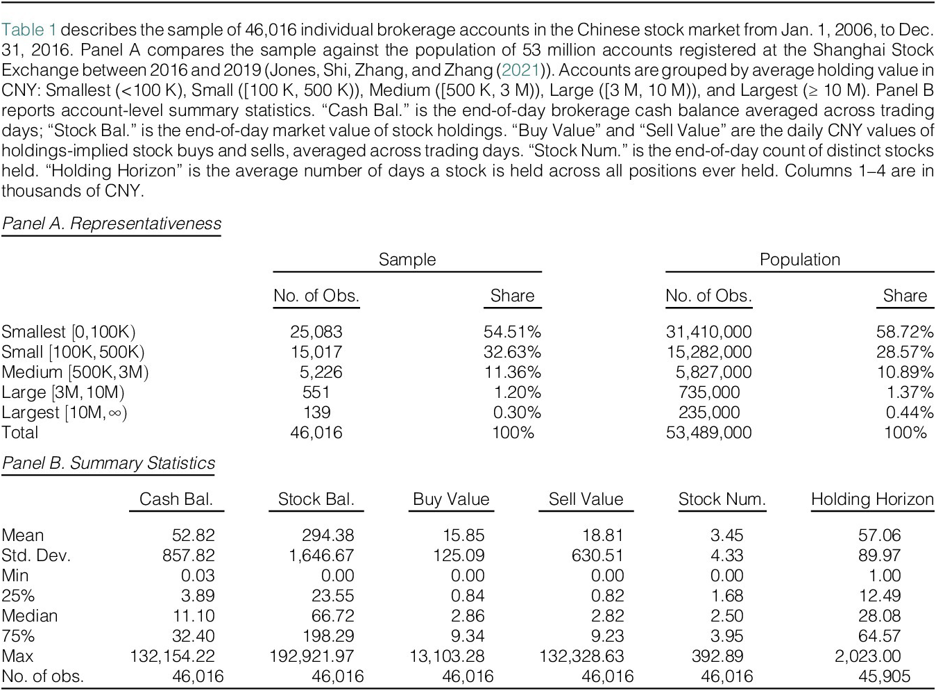
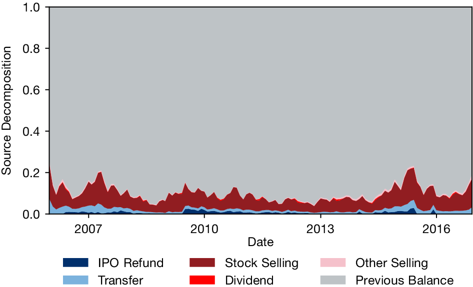


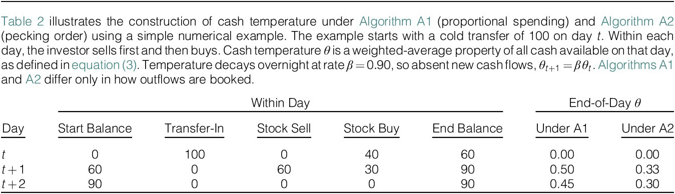
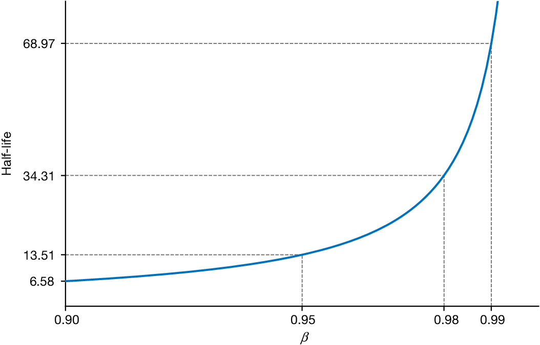


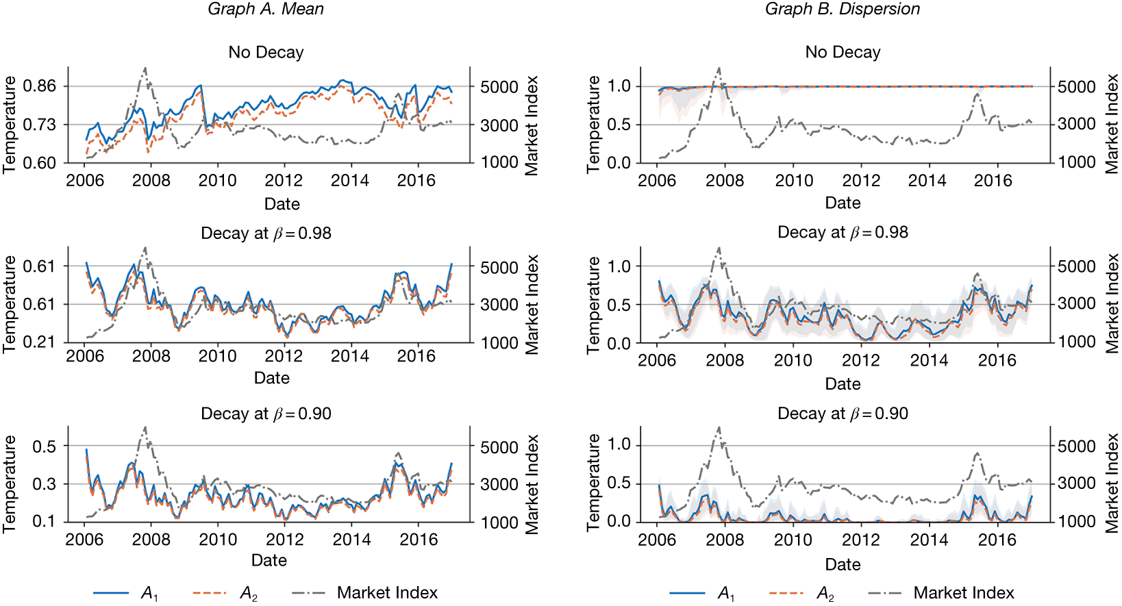


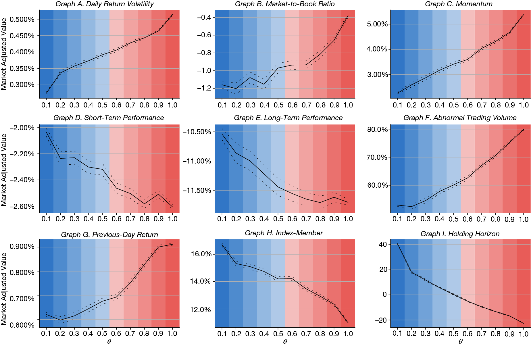


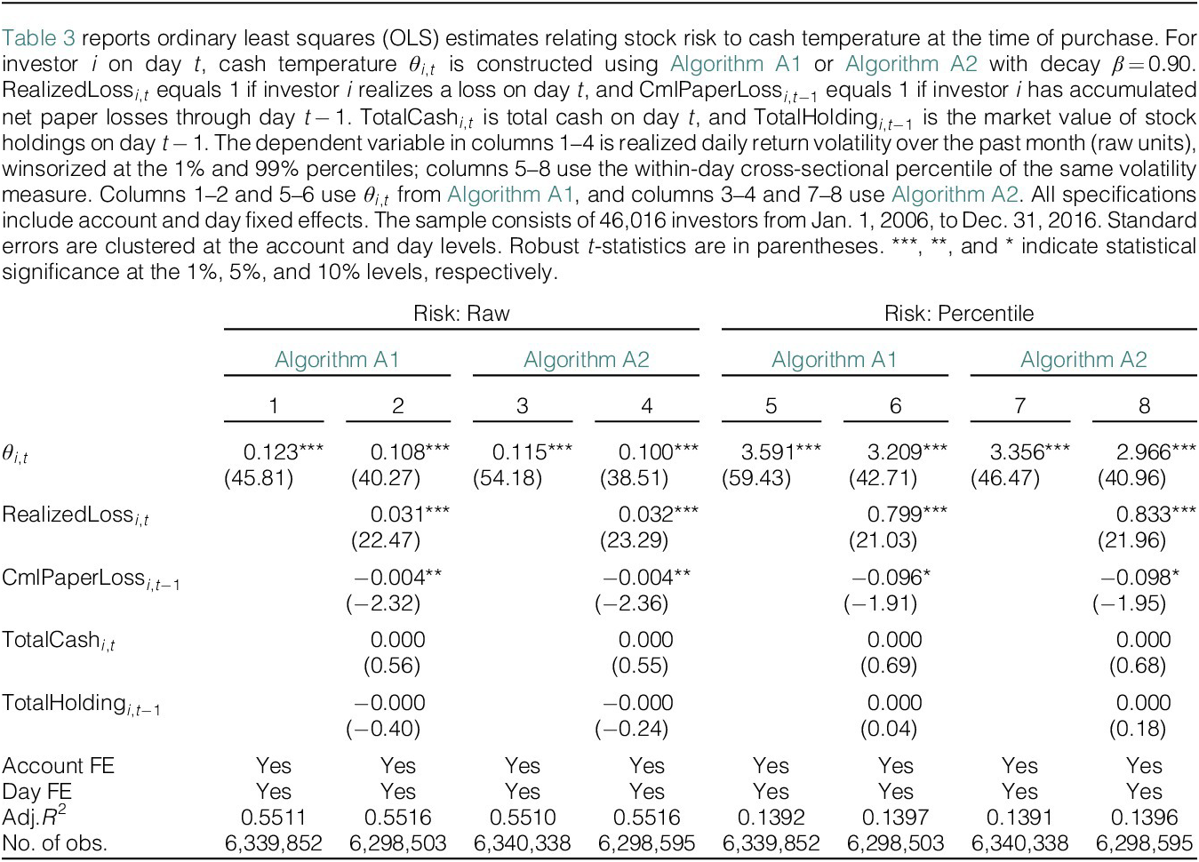
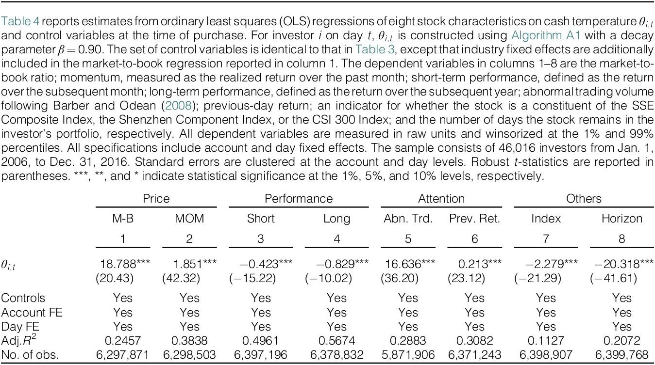
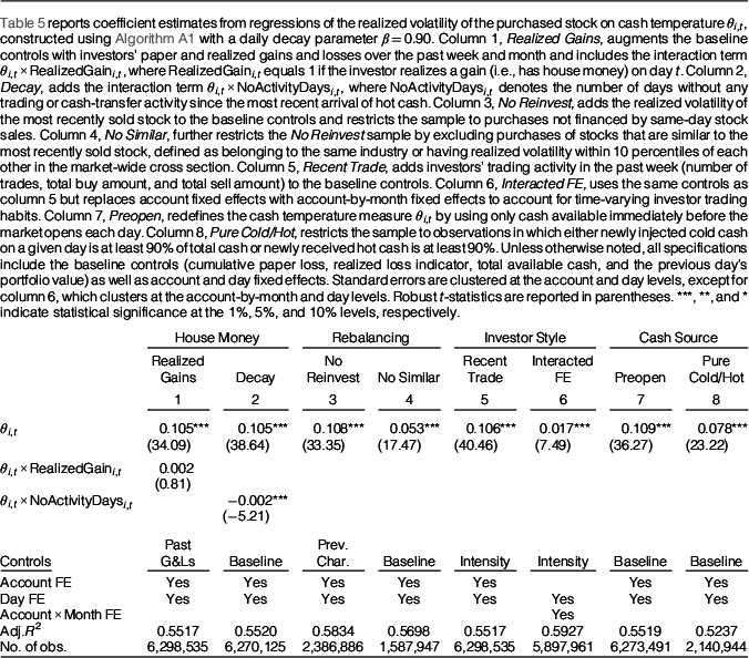
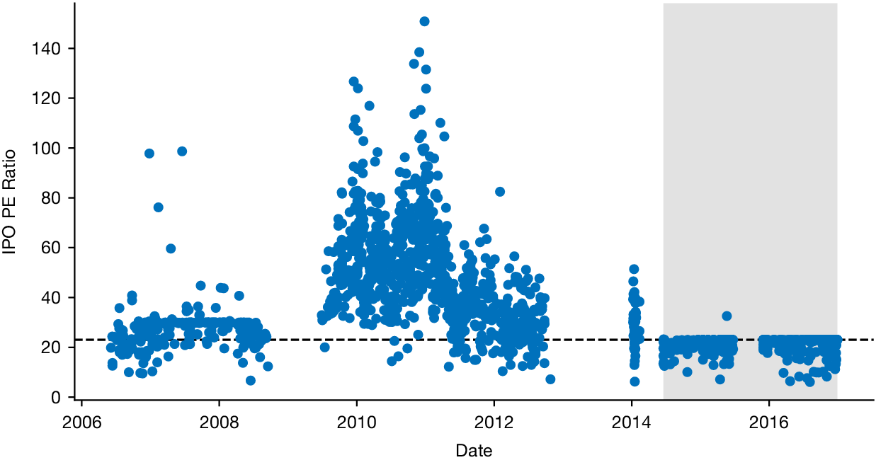
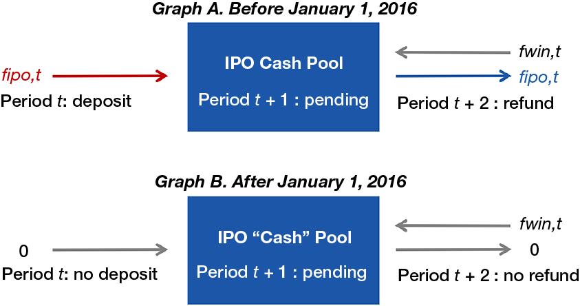


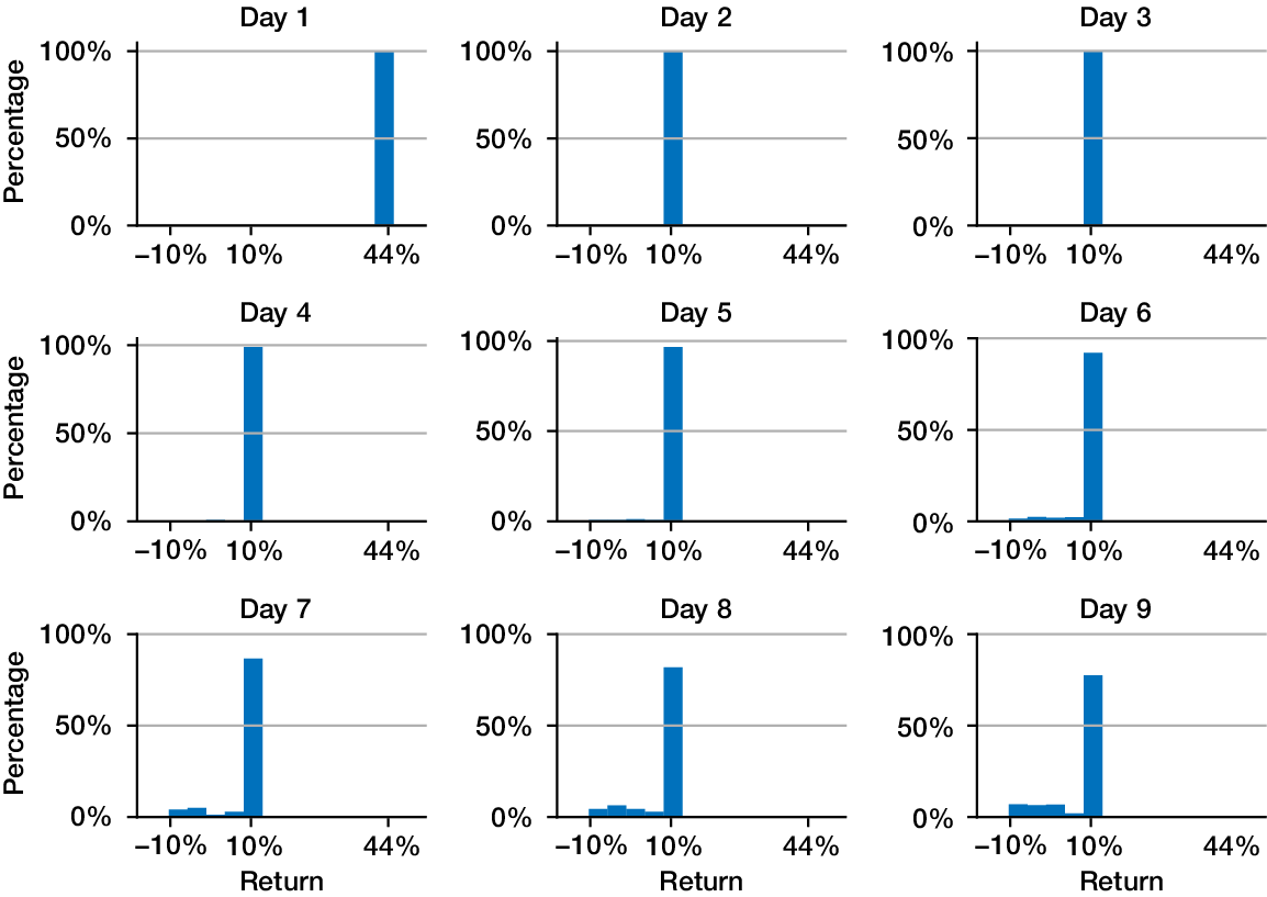

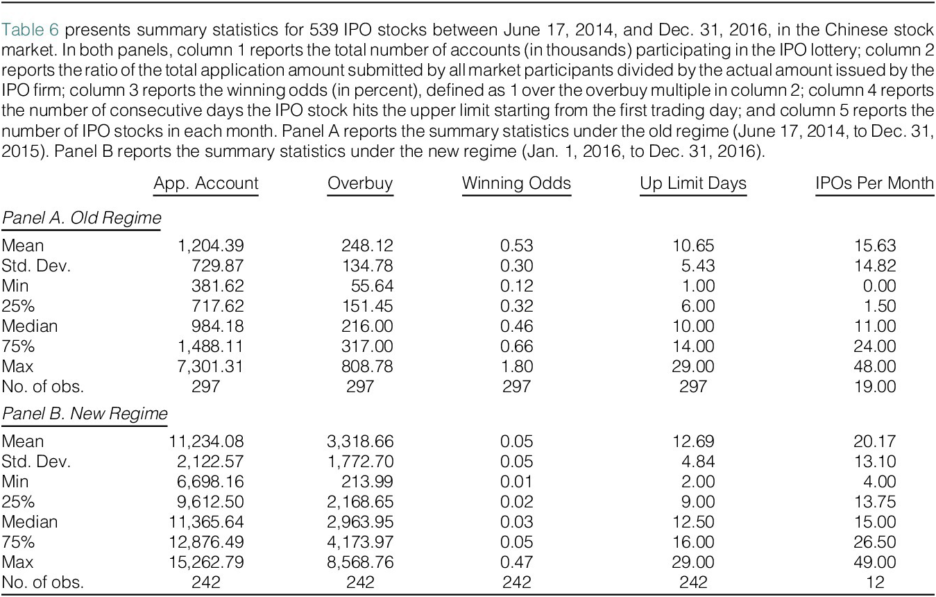
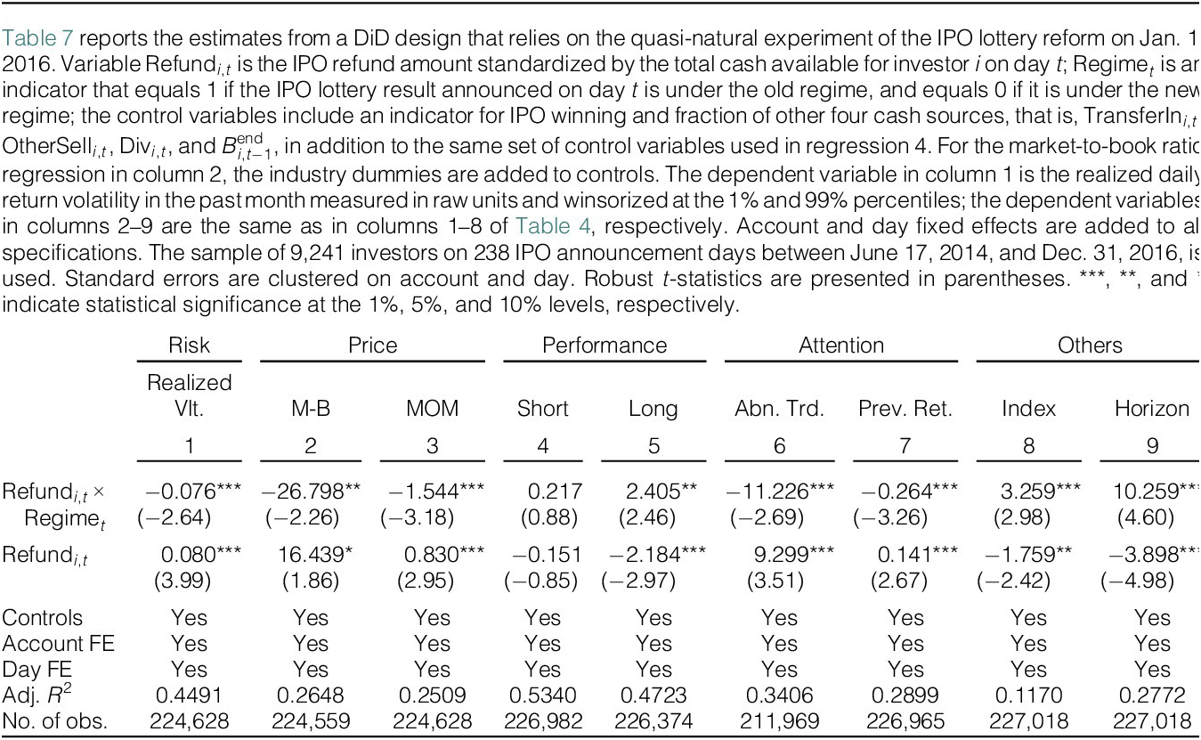
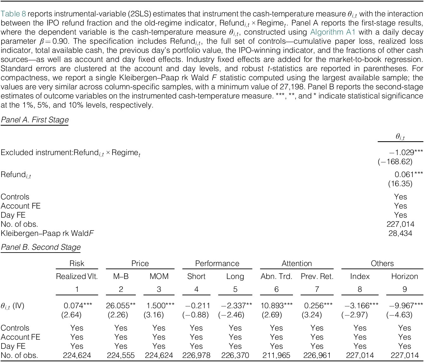
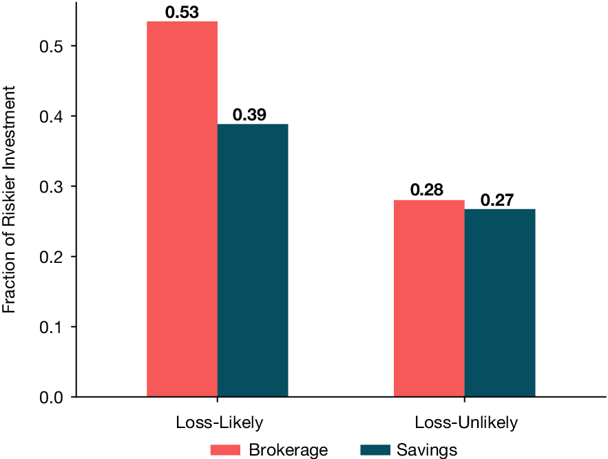
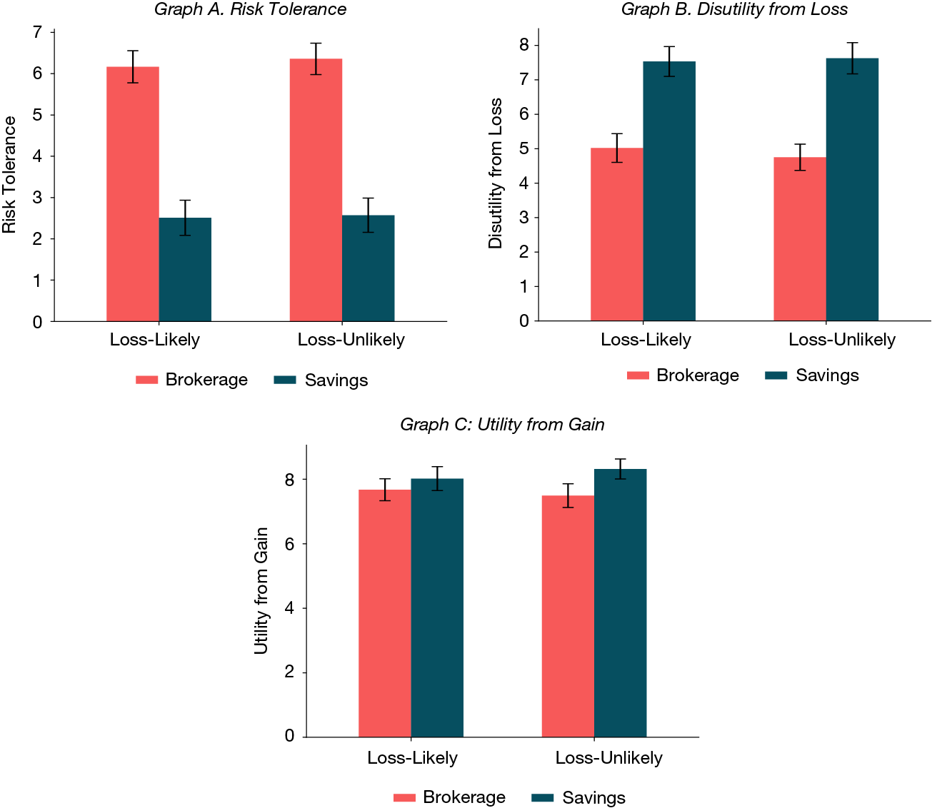
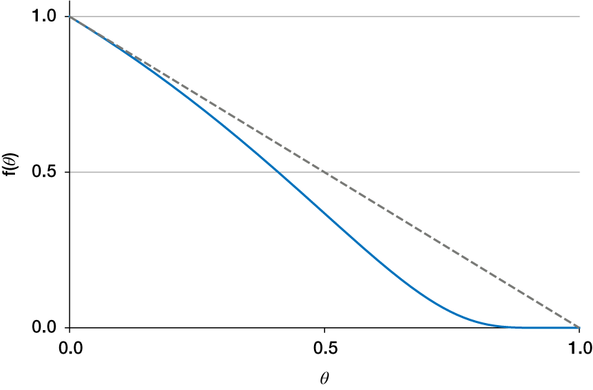


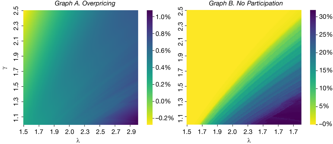


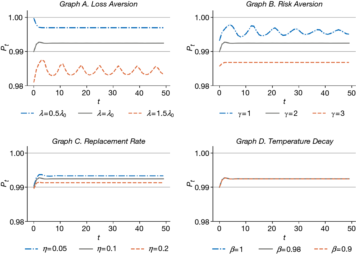


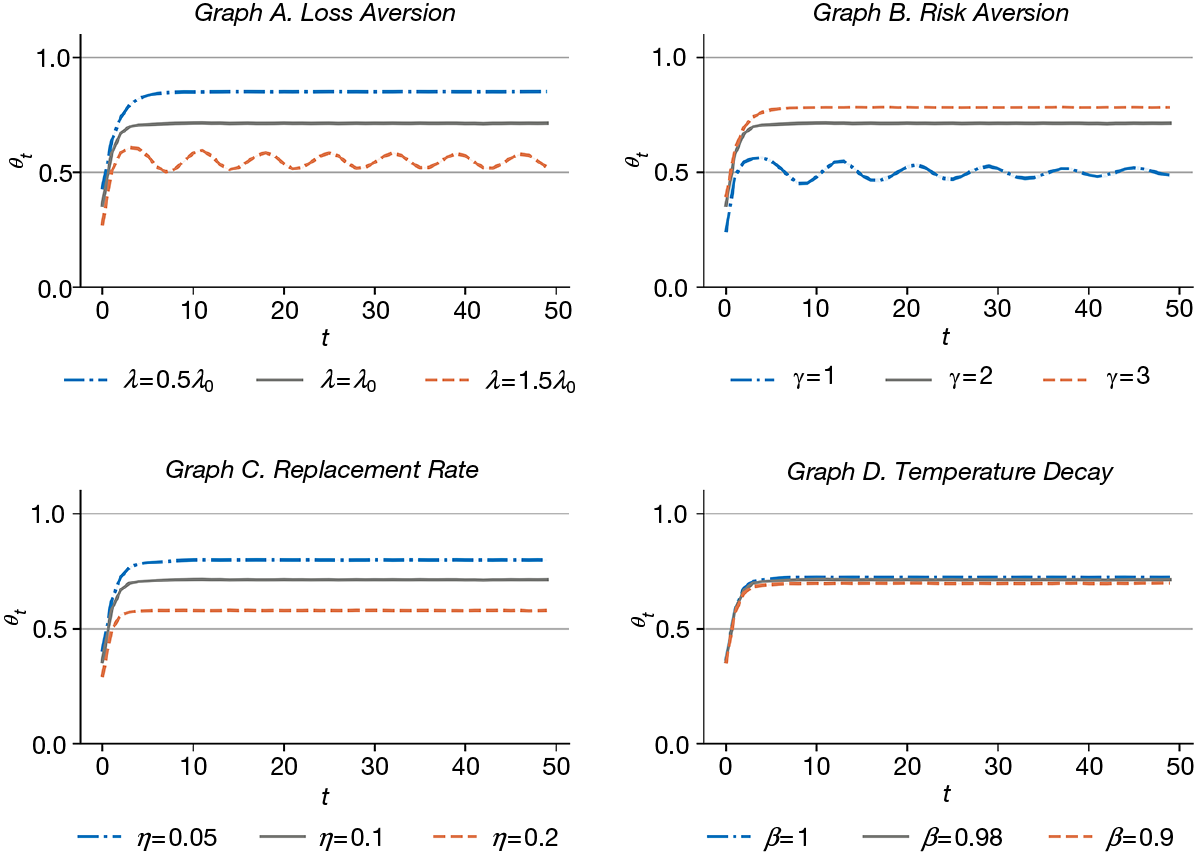
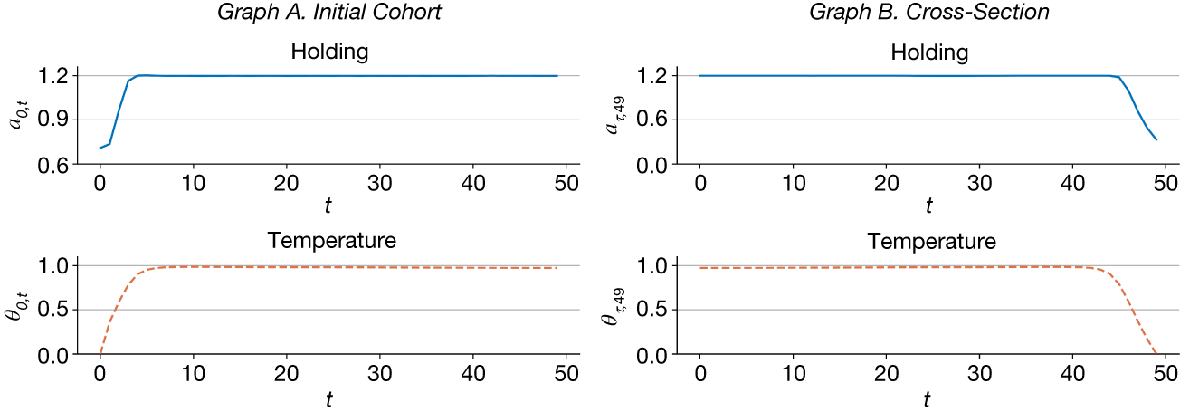


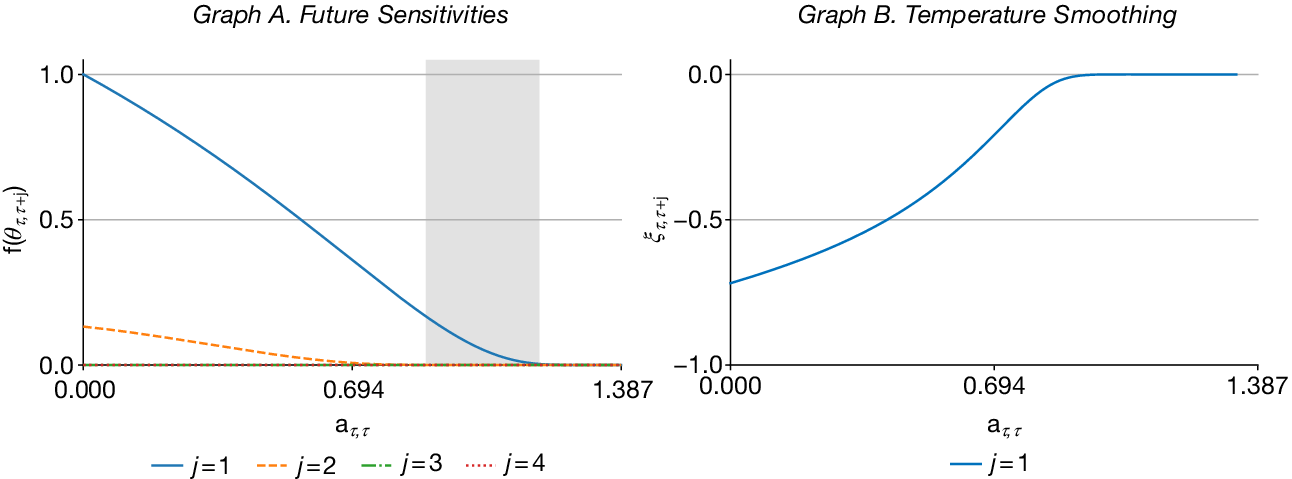


 Open access

