


1 Introduction
The dipole magnetic field generated by a current-carrying circular coil is an attractive confinement device for the study of electron–positron plasmas due to the unique stability and transport properties it affords the trapped plasma (Helander Reference Helander2014). In the near future, the first experiment aiming at this goal will be constructed (Pedersen et al. Reference Pedersen, Danielson, Hugenschmidt, Marx, Sarasola, Schauer, Schweikhard, Surko and Winkler2012). Recently, efficient injection and trapping of a cold positron beam in a dipole magnetic field configuration has been demonstrated by Saitoh et al. (Reference Saitoh, Stanja, Stenson, Hergenhahn, Niemann, Pedersen, Stoneking, Piochacz and Hugenschmidt2015) using a supported permanent magnet. This result is a key step towards further studies using a levitated magnetic coil with the ultimate aim of creating and studying of the first laboratory electron–positron plasmas.
In this paper, we present the results of the first gyrokinetic simulations of electron–positron plasmas in closed field-line systems, aiming to verify a number of theoretical predictions in the literature (Mishchenko, Plunk & Helander Reference Mishchenko, Plunk and Helander2018a) and extend these results to experimentally relevant geometries and parameter regimes.
It has been shown by Helander (Reference Helander2014) that pair plasmas possess unique gyrokinetic stability properties due to the mass symmetry between the particle species. For example, drift instabilities are completely absent in straight geometry, e.g. in a slab, provided that the density and temperature profiles of the two species are identical (‘symmetric’ pair plasmas). The symmetry between the two species is broken if the temperature profiles of the electrons and positrons differ or there is an ion contamination. In these regimes, drift instabilities can be excited even in unsheared slab geometry (Mishchenko et al. Reference Mishchenko, Zocco, Helander and Könies2018b). It has also been shown that instabilities can be excited when symmetry is broken through relaxation of the quasineutrality condition (Kennedy & Mishchenko Reference Kennedy and Mishchenko2019). In a sheared slab, pure pair plasmas are prone to current-driven reconnecting instabilities (Zocco Reference Zocco2017), but there are no drift waves. Note that asymmetry between the species is needed also in this case since the ambient electron flow velocity must differ from the positron one for the ambient current to be finite.
In contrast to slab geometry, a dipole magnetic field has finite curvature. In this case, the symmetry between the species is broken by curvature drifts and the plasma can be driven unstable by temperature and density gradients (Helander Reference Helander2014), even without ion contamination and for identical temperature profiles of the two species. This result also persists in the electromagnetic regime (Helander & Connor Reference Helander and Connor2016). The nonlinear stability of point-dipole pair plasmas has also been addressed (Helander Reference Helander2017) and it can be shown that turbulent transport ought to be largely absent. More recently, Mishchenko et al. (Reference Mishchenko, Plunk and Helander2018a) performed a detailed study of the gyrokinetic stability of pure pair plasma in both the Z-pinch and point-dipole limits. Again, it was found that such pair plasmas can be driven unstable by magnetic curvature, density and temperature gradients. In this paper, we validate these previous results through the use of a gyrokinetic code and, more importantly, show that many of the important stability results persist in the geometry and parameter regimes which will be used for the upcoming experiments.
In this paper, we use the gyrokinetic code GENE (Jenko et al. Reference Jenko, Dorland, Kotschenreuther and Rogers2000) to study the linear stability of electron–positron plasmas confined in a magnetic dipole. In § 2 we introduce the GENE code and the assumptions and modifications required to run simulations of pair plasmas in the dipole geometry. In § 3 we introduce the dipole geometry and the flux tubes which will be used in this study. Section 4 details some of the computational challenges involved in implementing the dipole geometry for use with GENE. In § 5 we show the results of simulations in an experimentally relevant dipole geometry introduced previously. There are many excellent theoretical studies of electron–ion plasmas in magnetic dipoles of both analytical and numerical flavours e.g. Krasheninnikov, Catto & Hazeltine (Reference Krasheninnikov, Catto and Hazeltine1999), Simakov, Hastie & Catto (Reference Simakov, Hastie and Catto2000b), Simakov et al. (Reference Simakov, Catto, Krasheninnikov and Ramos2000a), Garnier, Kesner & Mauel (Reference Garnier, Kesner and Mauel1999) and Kobayashi, Rogers & Dorland (Reference Kobayashi, Rogers and Dorland2010). These existing studies guide our search for the existence of the entropy mode and interchange mode, both of which have been shown to exist in electron–ion plasmas confined in dipole geometry. In § 6 we investigate the stability of such systems for different temperature gradients and density gradients. We show the results of numerical simulations for both the exact geometry and also the near-ring limit of the Z-pinch and draw comparisons between these results and the analytical results obtained in Mishchenko et al. (Reference Mishchenko, Plunk and Helander2018a). Section 7 is devoted to studying the stability of electron–positron plasmas in experimentally relevant conditions, for the first time exploring the stability of such plasmas in the regime where the Debye length is orders of magnitude larger than the gyroradius. We present our conclusions and outlook in § 7.
2 Physical assumptions
We will relegate a thorough discussion of laboratory pair plasmas to § 7 and will first focus our attention on electron–positron plasmas where the density of each species  $n_{s}$ is sufficiently large compared to the Brillouin density limit
 $$\begin{eqnarray}n_{s}\gg n_{Bs}:=\frac{\unicode[STIX]{x1D716}_{0}m_{s}\unicode[STIX]{x1D6FA}_{s}^{2}}{2e_{s}^{2}}.\end{eqnarray}$$
 Here,  $\unicode[STIX]{x1D716}_{0}$ is the vacuum permittivity, $m_{s}$ is the species rest mass, $\unicode[STIX]{x1D6FA}_{s}=e_{s}B/m_{s}$ the gyrofrequency, $B$ the magnitude of the magnetic field and $e_{s}$ the charge of each species. In this limit, Debye shielding effects can be neglected. Such densities, and indeed, such plasmas, are postulated to exist in astrophysics around compact high-energy density objects where copious pair creation can occur.
In contrast, for the first laboratory electron–positron plasma, the aim is to produce a symmetric pair plasma with species density in the range  $10^{12}~\text{m}^{-3}<n<10^{13}~\text{m}^{-3}$ and with a temperature $T$ between 1 and 10 eV. The Debye length $\unicode[STIX]{x1D706}_{D}=(\unicode[STIX]{x1D716}_{0}T/2ne^{2})^{1/2}$ for such plasmas will therefore be of the order of a few mm and will exceed the gyroradius $\unicode[STIX]{x1D70C}$ by two or three orders of magnitude provided the target magnetic field of approximately $B=1$ T is attained. A requirement for such a system to qualify as a plasma is that it contains many Debye lengths and therefore the gyroradius ought to be many orders of magnitude smaller than the macroscopic system length $L$, meaning that any microinstabilities ought to be well described by conventional gyrokinetic theory. That is, we are also declaring an interest in experimental plasmas satisfying the ordering $\unicode[STIX]{x1D70C}\ll \unicode[STIX]{x1D706}_{D}\ll L$. We note that such a plasma will not satisfy the ordering given in (2.1) as the Brillouin density $n_{Bs}\approx 10^{18}~\text{m}^{-3}$ will exceed the plasma density by several orders of magnitude.
In both of the scenarios we consider, the collision frequency is much larger than the inverse of the expected confinement time, yet much smaller than the frequency of typical microinstabilities. As such, it is reasonable to assume the local distribution function for each species will be Maxwellian, and that the plasma can be treated as being collisionless. Furthermore, a plasma with the parameters quoted above will have a very low value of  $\unicode[STIX]{x1D6FD}=4\unicode[STIX]{x1D707}_{0}nT/B^{2}$ and so throughout this paper we have considered only electrostatic simulations.
The GENE code can handle plasmas of different mass ratios by changing the mass of the lighter species (electrons). Electron–positron plasma is obtained when the mass of the electrons is equal to the mass of the singly charged ion species – thus obtaining charge asymmetry and a mass ratio of unity. Pair plasmas have already attracted some attention using the GENE code (Kennedy et al. Reference Kennedy, Mishchenko, Xanthopoulos and Helander2018) and are well benchmarked against similar gyrokinetic codes such as GS2 (Pedersen et al. Reference Pedersen, Boozer, Dorland, Kremer and Schmitt2003) and ORB5 (Horn-Stanja et al. Reference Horn-Stanja, Biancalani, Bottino and Mishchenko2019) which have been used to study electron–positron plasmas in a tokamak geometry. Here, we expand on existing studies by studying the gyrokinetics of pair plasma in experimentally relevant geometry for the first time.
In this work we will focus on electron–positron plasmas with the same temperature and density profiles and hence the species index,  $s$, will be supressed throughout the following exposition where appropriate.
3 Gyrokinetics of electron–positron plasmas
Electron–positron plasmas are well described by gyrokinetic theory. GENE is an Eulerian  $\unicode[STIX]{x1D6FF}f$ code which splits the full distribution of the gyrocentres into a static background equilibrium function $F_{0}$ plus a perturbation $g$. In this work, GENE is used to solve the normalised, linear, electrostatic gyrokinetic equation which, in field-line following coordinates ( $x,y,z$), can be written in the form
 $$\begin{eqnarray}\frac{\unicode[STIX]{x2202}g}{\unicode[STIX]{x2202}t}={\mathcal{L}}[g],\end{eqnarray}$$
with the linear operator
 $$\begin{eqnarray}\displaystyle {\mathcal{L}}[g] & = & \displaystyle -\left(\unicode[STIX]{x1D714}_{n}+\left(v_{\Vert }^{2}+\unicode[STIX]{x1D707}B_{0}-\frac{3}{2}\right)\unicode[STIX]{x1D714}_{T}\right)F_{0}\text{i}k_{y}\bar{\unicode[STIX]{x1D719}}+\frac{v_{\text{th}}}{JB_{0}}v_{\Vert }\unicode[STIX]{x1D6E4}_{z}\end{eqnarray}$$
 $$\begin{eqnarray}\displaystyle & & \displaystyle -\,\frac{T_{0}(2v_{\Vert }^{2}+\unicode[STIX]{x1D707}B_{0})}{e_{s}B_{0}}(K_{y}\unicode[STIX]{x1D6E4}_{y}+K_{x}\unicode[STIX]{x1D6E4}_{x})+\frac{v_{\text{th}}}{2JB_{0}}\unicode[STIX]{x1D707}\frac{\unicode[STIX]{x2202}}{\unicode[STIX]{x2202}z}\left(B_{0}\frac{\unicode[STIX]{x2202}g}{\unicode[STIX]{x2202}v_{\Vert }}\right).\end{eqnarray}$$
Details of the non-dimensionalisation can be found in Jenko et al. (Reference Jenko, Dorland, Kotschenreuther and Rogers2000) and references therein.
The auxiliary fields required by the code are
 $$\begin{eqnarray}\unicode[STIX]{x1D6E4}_{x,y}=\text{i}k_{x,y}g+\frac{e_{s}}{T_{0}}F_{0}\text{i}k_{x,y}\bar{\unicode[STIX]{x1D719}},\quad \unicode[STIX]{x1D6E4}_{z}=\frac{\unicode[STIX]{x2202}g}{\unicode[STIX]{x2202}z}+\frac{e_{s}}{T_{0}}F_{0}\frac{\unicode[STIX]{x2202}\bar{\unicode[STIX]{x1D719}}}{\unicode[STIX]{x2202}z},\end{eqnarray}$$
 with  $\bar{\unicode[STIX]{x1D719}}$ the gyroaveraged electrostatic potential, $B_{0}$ the equilibrium magnetic field and $k_{x}$ and $k_{y}$ are the components of the perpendicular wave vector. Other standard notation employed here is
 $$\begin{eqnarray}\unicode[STIX]{x1D707}=\frac{m(v_{x}^{2}+v_{y}^{2})}{2B_{0}},\quad v_{\text{th}}=\sqrt{\frac{2T_{0}}{m}}.\end{eqnarray}$$
 Besides the variation of the magnetic field, the most important equilibrium quantities entering the gyrokinetic equations are the gradient terms  $\unicode[STIX]{x1D714}_{n}$ and $\unicode[STIX]{x1D714}_{T}$ and the curvature terms $K_{x}$ and $K_{y}$. The role of these terms is elucidated below.
The gyrokinetic equation (3.1) is supplemented by Poisson’s equation for the electrostatic potential which reads
 $$\begin{eqnarray}\left(k_{\bot }^{2}\unicode[STIX]{x1D706}_{D}^{2}+\mathop{\sum }_{s}\frac{e_{s}^{2}}{T_{s}}n_{0s}(1-\unicode[STIX]{x1D6E4}_{0}(b_{s}))\right)\unicode[STIX]{x1D719}=\mathop{\sum }_{s}n_{0s}\unicode[STIX]{x03C0}e_{s}B_{0}\int \text{J}_{0}(\unicode[STIX]{x1D706}_{s})g_{s}\,\text{d}v_{\Vert }\,\text{d}\unicode[STIX]{x1D707},\end{eqnarray}$$
 where  $\text{J}_{0}$ is the Bessel function of the first kind, $\text{I}_{0}$ is the modified Bessel function of the first kind, $\unicode[STIX]{x1D6E4}_{0}(b_{s})=\exp (-b_{s})\text{I}_{0}(b_{s})$ and the dimensionless arguments of these functions are given by
 $$\begin{eqnarray}b_{s}=\frac{T_{s}m_{s}}{e_{s}^{2}B_{0}^{2}}k_{\bot }^{2},\quad \unicode[STIX]{x1D706}_{s}=\frac{v_{\text{th}}}{\unicode[STIX]{x1D6FA}_{s}}k_{\bot }\sqrt{B_{0}\unicode[STIX]{x1D707}}.\end{eqnarray}$$
3.1 Debye shielding and finite-Larmor-radius effects
Initially we will consider plasmas with very small Debye length  $k_{y}\unicode[STIX]{x1D706}_{D}\ll 1$. Under these conditions, the polarisation density response is the dominant term on the left-hand side of Poisson’s equation.
Later, in § 7, we will specialise to more experimentally relevant conditions and replace finite-Larmor-radius (FLR) effects with Debye shielding.
3.2 Density- and temperature-gradient terms in the gyrokinetic equation
In this work, we will focus on modes with length scales that are much smaller than those of the equilibrium quantities. As such, GENE is operated in a flux-tube mode, where a computational domain is constructed around a single magnetic field line and the profiles and gradients involved in the gyrokinetic equation are treated as constants.
Instabilities in pair plasmas are driven by a combination of density gradients, temperature gradients and magnetic curvature. The terms responsible for these features can easily be identified in the gyrokinetic equation (3.1). In our flux-tube geometry, the density and temperature gradients are given by
 $$\begin{eqnarray}\unicode[STIX]{x1D714}_{n}=\frac{a}{L_{n}}=-\frac{r_{\star }}{n_{0}}\frac{\text{d}n_{0}}{\text{d}x},\quad \unicode[STIX]{x1D714}_{T}=\frac{a}{L_{T}}=-\frac{r_{\star }}{T_{0}}\frac{\text{d}T_{0}}{\text{d}x}\end{eqnarray}$$
 and are assumed to be constant. Here,  $r_{\star }$ is a normalising length scale.
3.3 Geometric terms in the gyrokinetic equation
The geometry of the problem enters the gyrokinetic equation (3.1) through the terms  $K_{x}$ and $K_{y}$ which are combinations of dimensional factors involving elements of the metric tensor $\unicode[STIX]{x1D628}^{ij}$.
 $$\begin{eqnarray}K_{x}=-\frac{r_{\star }}{B_{\star }}\left(\frac{\unicode[STIX]{x2202}B_{0}}{\unicode[STIX]{x2202}y}+\frac{\unicode[STIX]{x1D6FE}_{1}}{\unicode[STIX]{x1D6FE}_{2}}\frac{\unicode[STIX]{x2202}B_{0}}{\unicode[STIX]{x2202}z}\right),\quad K_{y}=-\frac{r_{\star }}{B_{\star }}\left(\frac{\unicode[STIX]{x2202}B_{0}}{\unicode[STIX]{x2202}x}-\frac{\unicode[STIX]{x1D6FE}_{3}}{\unicode[STIX]{x1D6FE}_{1}}\frac{\unicode[STIX]{x2202}B_{0}}{\unicode[STIX]{x2202}z}\right),\end{eqnarray}$$
where the abbreviations
 $$\begin{eqnarray}\unicode[STIX]{x1D6FE}_{1}=\unicode[STIX]{x1D628}^{11}\unicode[STIX]{x1D628}^{22}-\unicode[STIX]{x1D628}^{21}\unicode[STIX]{x1D628}^{12},\quad \unicode[STIX]{x1D6FE}_{2}=\unicode[STIX]{x1D628}^{11}\unicode[STIX]{x1D628}^{23}-\unicode[STIX]{x1D628}^{21}\unicode[STIX]{x1D628}^{13},\quad \unicode[STIX]{x1D6FE}_{3}=\unicode[STIX]{x1D628}^{12}\unicode[STIX]{x1D628}^{23}-\unicode[STIX]{x1D628}^{22}\unicode[STIX]{x1D628}^{13},\end{eqnarray}$$
 for the geometric factors have been introduced. In this formulation  $x,y,\unicode[STIX]{x1D6FE}_{2}$ and $\unicode[STIX]{x1D6FE}_{3}$ are dimensional.
The geometry also plays a role through the inclusion of  $J$, the Jacobian matrix for the transformation between the polar coordinate representation $(r,\unicode[STIX]{x1D703},z)$ and the local flux-tube coordinates $(x,y,z)$ used by GENE. Furthermore, the variation of the magnetic field and its variation along the field line must also be supplied to GENE.
It is important to note that there are a number of freely scalable parameters inherent in the system of equations. Namely some appropriate length scale  $r_{\star }$ and magnetic field value $B_{\star }$ much be chosen in order to provide the metric quantities required by GENE in the appropriate normalisation. These normalising factors also appear in the equation for the Jacobian and magnetic field. The formulae for these quantities and details on the numerical implementation can be found in appendices A–B.
4 Implementation of the dipole geometry
The main focus of this work is on the simplest magnetic geometry for a pair-plasma experiment, namely that of a magnetic dipole. In practice, such a field will be created by passing a current through a levitated superconducting coil, the feasibility of which has previously been demonstrated in the levitated dipole experiment (Boxer et al. Reference Boxer, Bergmann, Ellsworth, Garnier, Kesner, Mauel and Woskov2010).
4.1 Magnetic flux tubes in dipole geometry
In standard cylindrical coordinates  $(r,\unicode[STIX]{x1D711},z)$ the magnetic field of a circular conducting loop with radius $r_{0}$ carrying a total current $I$ is given by
 $$\begin{eqnarray}\boldsymbol{B}(r,z)=\unicode[STIX]{x1D735}\unicode[STIX]{x1D713}(r,z)\times \unicode[STIX]{x1D735}\unicode[STIX]{x1D711},\quad \unicode[STIX]{x1D735}\unicode[STIX]{x1D711}=\frac{\boldsymbol{e}_{\unicode[STIX]{x1D711}}}{r},\end{eqnarray}$$
 with the poloidal magnetic flux  $\unicode[STIX]{x1D713}$ given by
 $$\begin{eqnarray}\unicode[STIX]{x1D713}(r,z)=\frac{\unicode[STIX]{x1D707}_{0}I}{2\unicode[STIX]{x03C0}}\sqrt{(r_{0}+r)^{2}+z^{2}}\left[\frac{r_{0}^{2}+r^{2}+z^{2}}{(r_{0}+r)^{2}+z^{2}}K(\unicode[STIX]{x1D705})-E(\unicode[STIX]{x1D705})\right],\end{eqnarray}$$
 where  $\unicode[STIX]{x1D707}_{0}$ is the permeability of free space and we have introduced the quantity
 $$\begin{eqnarray}\unicode[STIX]{x1D705}=\sqrt{\frac{4r_{0}r}{(r_{0}+r)^{2}+z^{2}}},\end{eqnarray}$$
and also the elliptic integrals of the first and second kind
 $$\begin{eqnarray}K(\unicode[STIX]{x1D705})=\int _{0}^{1}\frac{\text{d}x}{\sqrt{(1-x^{2})(1-\unicode[STIX]{x1D705}x^{2})}},\quad E(\unicode[STIX]{x1D705})=\int _{0}^{1}\frac{\sqrt{1-\unicode[STIX]{x1D705}x^{2}}}{\sqrt{1-x^{2}}}\,\text{d}x.\end{eqnarray}$$
 In order to construct the computational domain, an appropriate set of field-line following coordinates must be chosen. Denoting  $\unicode[STIX]{x1D713}_{\text{max}}$ the poloidal magnetic flux at the inner boundary and $\unicode[STIX]{x1D713}_{\text{min}}$ the poloidal flux at the outer boundary of the domain considered, we can choose convenient magnetic coordinates as follows:
 $$\begin{eqnarray}s=\frac{\unicode[STIX]{x1D713}-\unicode[STIX]{x1D713}_{\text{max}}}{\unicode[STIX]{x1D713}_{\text{min}}-\unicode[STIX]{x1D713}_{\text{max}}},\quad \unicode[STIX]{x1D703}=\frac{2\unicode[STIX]{x03C0}l}{L_{0}}-\unicode[STIX]{x03C0},\end{eqnarray}$$
 where  $l$ is the length along the flux tube and $L_{0}$ is the length of the field line. For a dipole magnetic field, $\unicode[STIX]{x1D703}$ is the field-line following coordinate.
From these quantities, one can calculate the various metric coefficients required by the GENE code in this coordinate system. The flux-tube geometry is then computed using a field-line tracing Runge–Kutta method to construct the required quantities at all points inside the flux-tube domain.
 $$\begin{eqnarray}\frac{\text{d}r}{\text{d}l}=\frac{B_{r}(r,z)}{B(r,z)}=b_{r},\quad \frac{\text{d}z}{\text{d}l}=\frac{B_{z}(r,z)}{B(r,z)}=b_{z},\quad r(0)=r_{c},\quad z(0)=0,\end{eqnarray}$$
 where  $l$ is the length measured along the field line and $r_{c}$ labels the chosen flux surface.
The advantage of this implementation is the freedom to consider a number of different flux tubes, using the radial distance,  $r_{c}=c_{\star }r_{0}$ to the point where the field line crosses the equatorial plane as a free parameter (i.e. varying
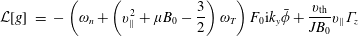
  $c_{\star }$). The magnetic field lines relevant to our studies are shown in figure 1. The central field line is located near the bulk of an expected electron positron plasma and is characterised by a reasonably strong magnetic field variation along the field line $B_{\text{max}}/B_{\text{min}}\approx 5$. Hereafter, we will refer to the flux tube surrounding this field line as the ‘dipole flux tube’.
Illustrative example of a single magnetic field line (a) and the variation of the magnetic field strength along the field line (b) for different values of the parameter  $r_{c}$. As this parameter is varied we can change the flux tube from one resembling a Z-pinch geometry to one resembling a point-dipole limit.
We are also able to make great use of the freedom afforded to us to consider simulations using different field-line geometries. We are able to increase the value of  $r_{c}$ and push towards the far field limit in which the magnetic field line approaches that of a point dipole with a much stronger variation of the magnetic field along the field line $B_{\text{max}}/B_{\text{min}}\approx 20$ and beyond. This is a useful feature and can give us an understanding of how the geometry affects the various properties of the system. Pushing the geometry to these extreme limits comes with its own fair share of computational challenges described below.
Another limiting case to which we will pay particular attention is that of the near-ring limit. As we approach the superconducting ring, the parallel variations and trapped particles become negligible and the field lines become circular. As a result, the system becomes approximately equivalent to that of a Z-pinch. This is a particularly important limit for two main reasons. Firstly, an exact Z-pinch geometry has already been implemented in GENE by Navarro, Teaca & Jenko (Reference Navarro, Teaca and Jenko2016) and has been used in studies of electron–ion plasmas. This geometry allows us to benchmark our dipole geometry against these existing results for an electron–ion plasma and also provides us with an exact Z-pinch for electron–positron studies, noting that whilst our geometry can come very close to an exact Z-pinch  $B_{\text{max}}/B_{\text{min}}\approx 1.016$, we cannot reach this point exactly as the coordinate transforms become singular leading to difficulties in the code (this can be seen from a near-zero Jacobian in figures 2 and 3). Secondly, a tractable analytic theory of linear stability in the Z-pinch limit exists (Mishchenko et al. Reference Mishchenko, Plunk and Helander2018a), once again allowing us to benchmark both our geometry and the physics aspects of electron–positron simulations.
4.2 Computational challenges with the dipole geometry
During the implementation of the dipole geometry in the GENE code, several issues were encountered pertaining to time-stepping and convergence issues within the code, as well as a dependence on certain computational libraries.
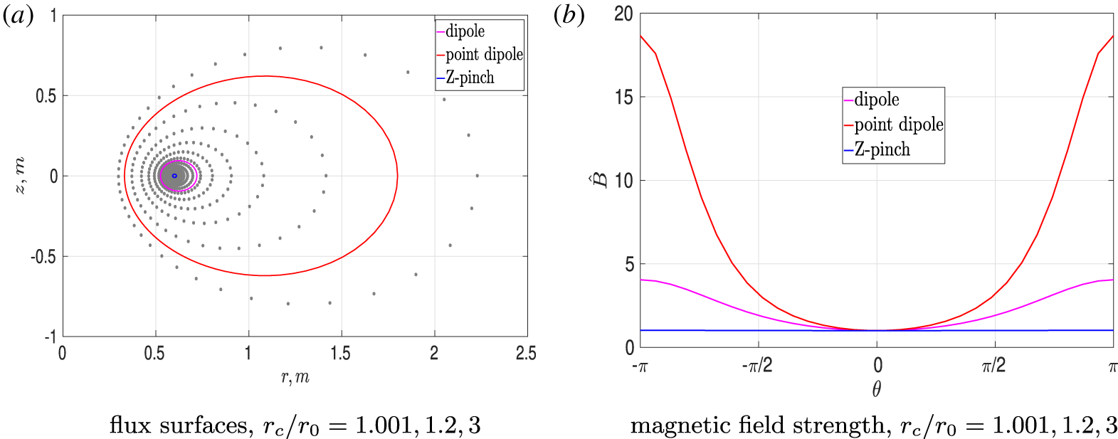
Variation of the magnetic field strength (a) and the Jacobian (b) for the three different flux tubes. The magnetic field strength is normalised to the inboard midplane.
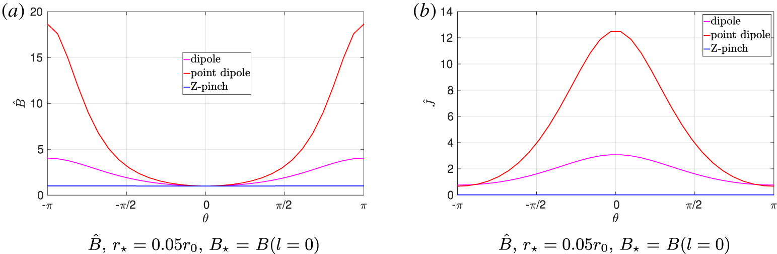
Variation of the magnetic field strength (a) and the Jacobian (b) for the three different flux tubes. The magnetic field strength is normalised to the outboard midplane.
Firstly, in order to probe different flux tubes, the code must be capable of calculating the different metric quantities at different points in space: both very close and very far to the current-carrying ring. In order to avoid the use of external libraries, the Elliptic integrals were estimated as a sum of rational functions through use of the Padé approximation (Luke Reference Luke1968). That is, the approximations
 $$\begin{eqnarray}K(\unicode[STIX]{x1D705})\approx \frac{\unicode[STIX]{x03C0}}{2}k_{4}(\unicode[STIX]{x1D705}),\quad E(\unicode[STIX]{x1D705})\approx g_{3}(\unicode[STIX]{x1D705}),\end{eqnarray}$$
where
 $$\begin{eqnarray}k_{4}(x):=\frac{1}{5}+\frac{8(8-5\unicode[STIX]{x1D705}^{2})}{25(5(2-\unicode[STIX]{x1D705}^{2})^{2}-4)}+\frac{64(32-5\unicode[STIX]{x1D705}^{2})}{25(5(8-\unicode[STIX]{x1D705}^{2})^{2}-64)}+\frac{128(16-5\unicode[STIX]{x1D705}^{2})}{25(5(16-\unicode[STIX]{x1D705}^{2})^{2}-1024)}\end{eqnarray}$$
and
 $$\begin{eqnarray}\displaystyle g_{3}(\unicode[STIX]{x1D705}) & := & \displaystyle \frac{1}{8}+\frac{32-4\unicode[STIX]{x1D705}^{2}}{\unicode[STIX]{x1D705}^{4}-32\unicode[STIX]{x1D705}^{2}+128}+\frac{8-2\unicode[STIX]{x1D705}^{2}}{\unicode[STIX]{x1D705}^{4}-16\unicode[STIX]{x1D705}^{2}+32}+\frac{4-3\unicode[STIX]{x1D705}^{2}}{4(\unicode[STIX]{x1D705}^{4}-8\unicode[STIX]{x1D705}^{2}+8)}\nonumber\\ \displaystyle & & \displaystyle -\,\frac{\unicode[STIX]{x1D705}^{3}-8\unicode[STIX]{x1D705}^{2}+32}{2(\unicode[STIX]{x1D705}^{4}-16\unicode[STIX]{x1D705}^{3}+64\unicode[STIX]{x1D705}^{2}-128)}+\frac{\unicode[STIX]{x1D705}^{3}+8\unicode[STIX]{x1D705}^{2}-32}{2(\unicode[STIX]{x1D705}^{4}+16\unicode[STIX]{x1D705}^{3}+64\unicode[STIX]{x1D705}^{2}-128)}\end{eqnarray}$$
were employed.
These approximations introduce an error in each of the metric quantities required by GENE. Typically, this error is too small to calculate accurately, further details can be found in Luke (Reference Luke1968).
Secondly, there were a number of computational issues relating to the appropriate choice of normalisation for each of the metric quantities required by GENE. The metric elements required had to first be normalised to some appropriate reference length scale  $r_{\star }$ and some appropriate reference magnetic field strength $B_{\star }$. An inherent feature in the dipole geometry is that the magnetic field strength can vary along the field line by orders of magnitude and similarly the length scales in the problem can vary by an order of magnitude when we are interested in pushing the geometry very close to, or very far from, the current-carrying coil. As such, certain choices of normalisation lead to either very large or very small values for each of the metric quantities.
In particular, issues were found when the choice of normalisation led to the transformation between cylindrical coordinates and the field-line following coordinates having a normalised Jacobian  $\hat{J}=J/(B_{\star }r_{\star })$ or a magnetic field $\hat{B}=B/B_{\star }$ variation many orders of magnitude smaller or larger than would be found in say a tokamak or stellarator. This led to time-stepping issues in the code which uses an adaptive time-stepping scheme based on the value of the Jacobian. The variations of the normalised magnetic field strength and the Jacobian along the flux tube for different normalisations can be seen in figures 2 and 3.
4.3 Numerical set-up
Henceforth, we will consider only two flux-tube geometries: (i) The ‘dipole flux tube’ with  $r_{c}=1.2r_{0}$. This field line has a moderate variation of the magnetic field along the flux tube. We take the normalisation as detailed in figure 2, which has a moderate variation of both $\hat{B}$ and $\hat{J}$ along the field line. (ii) The exact Z-pinch geometry of (Navarro et al. Reference Navarro, Teaca and Jenko2016). For convenience, the relevant parameters which need to be supplied to GENE in order to construct the flux tube are shown in table 1.

In this work, GENE is operated using the eigenvalue solver (Roman et al. Reference Roman, Kammerer, Merz and Jenko2009) to analyse the spectrum of the linear gyrokinetic operator given in (3.3). Spectral transforms are then used to return the eigenvalue associated with the most unstable mode. Interestingly, we often found two ‘most unstable’ modes (two instabilities with the same growth rate, propagating in opposite directions).
The numerical resolution in the field-line following direction is 128 grid points, while 16 and 8 grid points are employed for the parallel velocity and magnetic moment directions respectively. GENE employs numerical dissipation (hyperdiffusion) in order to retain physicality of the simulation results. The need for these terms arises from numerical effects, such as zigzag-like mode growth, due to the finite difference schemes employed by the code. In this work, we employ a hyperdiffusion in the parallel direction in both physical space  $D_{4}^{\Vert }$ and in velocity space $D_{4}^{v_{\Vert }}$. Hyperdiffusion is included by adding terms involving higher-order derivatives to the differential operator in the gyrokinetic equation
 $$\begin{eqnarray}D_{4}^{\Vert }=-\unicode[STIX]{x1D716}_{\Vert }\left(\frac{\unicode[STIX]{x0394}z}{2}\right)^{4}\unicode[STIX]{x1D6FB}_{\Vert }^{4},\quad D_{4}^{v_{\Vert }}=-\unicode[STIX]{x1D716}_{v_{\Vert }}\left(\frac{\unicode[STIX]{x0394}v_{\Vert }}{2}\right)^{4}\frac{\unicode[STIX]{x2202}^{4}}{\unicode[STIX]{x2202}v_{\Vert }^{4}}.\end{eqnarray}$$
 We have set the strength of the hyperdiffusion to  $\unicode[STIX]{x1D716}_{v_{\Vert }}=0.2$ for the parallel velocity and to $\unicode[STIX]{x1D716}_{\Vert }=0.25$ in the parallel direction, guided by the studies performed by Pueschel, Dannert & Jenko (Reference Pueschel, Dannert and Jenko2010). We also performed simulations employing different hyperdiffusivity values and found no considerable change in the results.
5 Instabilities in the dipole system
We have performed the first linear simulations of electron–positron plasmas in dipole geometry with an intermediate variation of the magnetic field along the flux tube. It is perhaps pertinent to start this section with a caution, electron–positron plasmas do indeed posses remarkable stability properties and there are many examples one could show of stable pair plasmas for a range of different parameters. In this section we will focus entirely on unstable cases in order to demonstrate the different modes which exist in such plasmas.
5.1 Linear instabilities, entropy and interchange modes
Based on work done previously by Simakov et al. (Reference Simakov, Hastie and Catto2000b) and Kobayashi et al. (Reference Kobayashi, Rogers and Dorland2010) we anticipate finding two main instabilities in a ring dipole system, namely interchange mode at large scales and entropy modes at smaller scales. Both of these instabilities are driven by a combination of temperature gradients, density gradients and magnetic curvature.
One can see the transition between the two modes by performing a scan over  $k_{y}\unicode[STIX]{x1D70C}$ in an unstable parameter region. In figure 4 we show the results of such a scan. Immediately clear is the transition between the two types of modes occurring around $k_{y}\unicode[STIX]{x1D70C}\approx 0.3$ in the Z-pinch case and around $k_{y}\unicode[STIX]{x1D70C}\approx 3$ in the dipole case. It is not surprising that there is a large discrepancy in the numerical values $k_{y}\unicode[STIX]{x1D70C}$ where this transition occurs between the two geometries, this was also observed by Kobayashi et al. (Reference Kobayashi, Rogers and Dorland2010) and is due to the choice of normalisation. Given an appropriate normalisation of the dipole geometry, the two plots can be made both qualitatively and quantitatively similar.
We also remark that our simulations also obey the results found in Kennedy et al. (Reference Kennedy, Mishchenko, Xanthopoulos and Helander2018) that the most unstable mode is purely growing i.e. has zero frequency.
We observe qualitatively similar results when comparing between the dipole and Z-pinch cases. This is similar to what was observed for conventional plasmas by Kobayashi et al. (Reference Kobayashi, Rogers and Dorland2010) using the gyrokinetic code GS2 and the numerical differences can be traced back to differences in normalisation. A similar result can also be found by solving the dispersion relation in the Z-pinch case (Mishchenko et al. Reference Mishchenko, Plunk and Helander2018a).
5.2 Implications for nonlinear pair-plasma studies
Of much interest for the experimental campaign will be studies of the turbulence and transport in pair plasmas confined in closed field-line geometries. The GENE code has been used extensively to study nonlinear physics in fusion plasmas in standard geometries, but we believe that the mode spectra obtained here suggest that the local flux-tube model we have employed will not be sufficient for nonlinear studies in the dipole.
The problematic peaking of the mode spectra for very small  $k_{y}\unicode[STIX]{x1D70C}$ (as seen in figure 4) has also been observed in fusion plasmas for kinetic ballooning mode (KBM) studies. In the KBM case this spectral feature leads to issues of saturation and resolution in turbulence studies. Recently, it was shown (Ishizawa et al. Reference Ishizawa, Imadera, Nakamura and Kishimoto2019) that the use of a global code can overcome these issues and it is our hope that this is also the case for studies of electron–positron plasmas.
It seems that despite the mass-ratio simplification, the nonlinear theory of electron–positron plasma confinement in a magnetic dipole is a complex non-local multi-scale problem. In the future, this should be addressed through the implementation of a global dipole geometry in a gyrokinetic code such as GENE.
Growth rate  $\unicode[STIX]{x1D6FE}$ and real frequency $\unicode[STIX]{x1D714}$ plotted as a function of $k_{y}\unicode[STIX]{x1D70C}_{i}$ for different flux tubes. Note the different ordinate scales due to the different length scales introduced by the choice of normalisation.

6 Linear stability in parameter space
Of primary interest from an experimental perspective, is the validation of several analytical studies which predict superb linear stability properties in large regions of temperature-gradient, density-gradient space. Often, these analytical predictions are obtained by taking suitable asymptotic limits of the dipole geometry in order to obtain a tractable gyrokinetic theory.
6.1 Comparison with dispersion relation
In order to benchmark our stability studies we first turn our attention to the Z-pinch geometry in order to make comparisons to the theory obtained by Mishchenko et al. (Reference Mishchenko, Plunk and Helander2018a). This is also an experimentally relevant geometry. In the region close to the current loop, the dipole magnetic field is approximately that of a Z-pinch.
 $$\begin{eqnarray}\frac{r-r_{0}}{r_{0}}\sim \frac{z}{r_{0}}\sim \frac{\unicode[STIX]{x1D70C}}{r_{0}}\ll 1.\end{eqnarray}$$
In this regime, one can take field-line average of the linear gyrokinetic equation and perform the velocity space integrals analytically in order to obtain the dispersion relation
 $$\begin{eqnarray}1+k_{\bot }^{2}\unicode[STIX]{x1D706}_{D}^{2}=\frac{1}{2}(D_{+}+D_{-}),\quad D_{\pm }=\frac{1}{\sqrt{\unicode[STIX]{x03C0}}}\int \frac{\unicode[STIX]{x1D6FA}\mp \unicode[STIX]{x1D6FA}_{\star }^{T}}{\unicode[STIX]{x1D6FA}\mp x_{\bot }^{2}/2\mp x_{\Vert }^{2}}\exp (-x^{2})x_{\bot }\,\text{d}x_{\bot }\,\text{d}x_{\Vert },\end{eqnarray}$$
 where we have adopted the notation of Mishchenko et al. (Reference Mishchenko, Plunk and Helander2018a) and introduced  $\unicode[STIX]{x1D714}_{d}=\hat{\unicode[STIX]{x1D714}}_{d}(x_{\Vert }^{2}+x_{\bot }^{2}/2),\unicode[STIX]{x1D6FA}=\unicode[STIX]{x1D714}/\hat{\unicode[STIX]{x1D714}}_{d},x=\sqrt{x_{\Vert }^{2}+x_{\bot }^{2}},\unicode[STIX]{x1D6FA}_{\star }^{T}=\unicode[STIX]{x1D714}_{\star }^{T}/\hat{\unicode[STIX]{x1D714}}_{d}=\unicode[STIX]{x1D6FA}_{\star }[1+\unicode[STIX]{x1D702}(x^{2}-3/2)],\unicode[STIX]{x1D702}=\text{d}\ln T/\text{d}\ln n$ and $\unicode[STIX]{x1D6FA}_{\star }=\unicode[STIX]{x1D714}_{\star }/\hat{\unicode[STIX]{x1D714}}_{d}$. This dispersion relation can be solved numerically in order to probe the linear instability features.
In this paper we will be primarily interested in limits of this equation where we are able to deduce regions of linear stability in  $(\unicode[STIX]{x1D714}_{\star },\unicode[STIX]{x1D714}_{\star }^{T})$ space. At $k_{\bot }\unicode[STIX]{x1D706}_{D}\lesssim 1$, the fluid limit $\unicode[STIX]{x1D6FA}\gg 1$ can be applied to (6.2) and from this equation we can deduce the ‘fluid instability condition’ which states that we require
 $$\begin{eqnarray}\frac{\unicode[STIX]{x1D714}_{\star }}{\hat{\unicode[STIX]{x1D714}}_{d}}(1+\unicode[STIX]{x1D702})>\frac{7}{4}\end{eqnarray}$$
for an instability.
One can also use equation (6.2) to derive the ‘resonant stability boundary’ (Mishchenko et al. Reference Mishchenko, Plunk and Helander2018a) by taking  $\unicode[STIX]{x1D6FA}\rightarrow 0$ to obtain
 $$\begin{eqnarray}\frac{\unicode[STIX]{x1D714}_{\star }}{\hat{\unicode[STIX]{x1D714}}_{d}}(1-\unicode[STIX]{x1D702})=\frac{1+k_{\bot }^{2}\unicode[STIX]{x1D706}_{D}^{2}}{\unicode[STIX]{x03C0}}.\end{eqnarray}$$
Having obtained a complete linear stability map for electron–positron plasmas in a Z-pinch analytically, we are now provided with an opportunity to benchmark electron–positron plasma simulations using the existing Z-pinch geometry implemented in GENE.
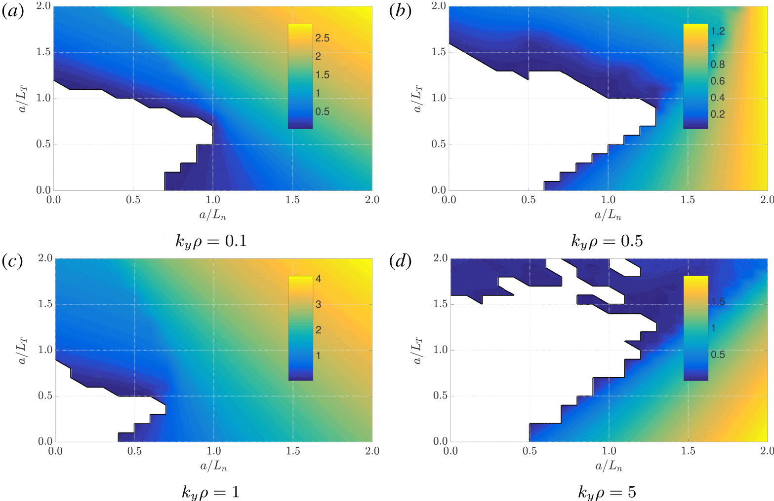
Stability diagram for several values of  $k_{\bot }\unicode[STIX]{x1D706}_{D}$, (a–c), computed by solving the dispersion relation (these figures are reproduced from Mishchenko et al. (Reference Mishchenko, Plunk and Helander2018a) with permission). Also shown are the stability diagrams for several values of $k_{\bot }\unicode[STIX]{x1D70C}_{s}$, (d–f), this time calculated using GENE. Theoretical stability boundaries are also shown in each figure. The colour of the density plot corresponds to numerically obtained growth rate. The region of stability bordered by a solid black contour in each case. We note the outstanding agreement between the use of GENE and the previous results using the linear dispersion relation. In the second set of stability diagrams, $k_{\bot }\unicode[STIX]{x1D70C}_{s}$ is playing the role of $k_{\bot }\unicode[STIX]{x1D706}_{D}$, which is set to zero in GENE. The theoretical stability lines (dashed red, and dashed green) correspond respectively to (6.3) and (6.4). Once again we note that that the deviation from the red theoretical stability boundary (which does not include finite- $k_{\bot }\unicode[STIX]{x1D70C}_{s}$ corrections) decreases as $k_{\bot }^{2}\unicode[STIX]{x1D70C}_{s}^{2}\rightarrow 0$, although surprisingly slowly. In the GENE simulations, the region of stability is white and is bordered by a solid black contour.

In figure 5 we reproduce the results of solving the dispersion relation (6.2) from Mishchenko et al. (Reference Mishchenko, Plunk and Helander2018a). Also in figure 5 we show the same stability diagram obtained from linear gyrokinetic simulations with GENE. The agreement shown is remarkable. GENE is able to fully capture the linear stability features for the exact Z-pinch.
6.2 Comparison with the ring dipole
Of more interest to us, is the comparison of the linear stability diagram obtained from the Z-pinch to the more experimentally realistic geometries of our dipole flux tube. We can also investigate how the features of the stability diagram change depending on whether we are in the low or high  $k_{y}$ branch of the instability.
We show the stability diagrams for the low and high  $k_{y}$ branches for (i) the ring dipole and (ii) the Z-pinch in figure 6. As before, the qualitative features of each of the stability diagrams is the same in each $k_{y}$ regime, with the difference in growth rates, gradients and $k_{y}\unicode[STIX]{x1D70C}$ values being once again due to the differences in normalisation. In these instances, the values $k_{y}\unicode[STIX]{x1D70C}$ are chosen from the scans detailed for example in figure 4. In each geometry we see that we are able to capture the stability triangle in the lower left-hand corner.
It is also important to point out that the stability diagram scales with the value of  $k_{y}\unicode[STIX]{x1D70C}$. From Mishchenko et al. (Reference Mishchenko, Plunk and Helander2018a) (their equation (5.25)) we see that, the dispersion relation for the point dipole, in the limit $\unicode[STIX]{x1D714}/2\tilde{\unicode[STIX]{x1D714}}_{d}\rightarrow \infty$, becomes
 $$\begin{eqnarray}\unicode[STIX]{x1D714}^{2}=-\frac{2\tilde{\unicode[STIX]{x1D714}}_{d}^{2}}{\langle k_{\bot }^{2}\unicode[STIX]{x1D706}_{d}^{2}\rangle }\left[\frac{\unicode[STIX]{x1D714}_{T}+\unicode[STIX]{x1D714}_{n}}{\tilde{\unicode[STIX]{x1D714}}_{d}}-5\right],\end{eqnarray}$$
 where  $\tilde{\unicode[STIX]{x1D714}}_{d}$ is the bounce-averaged drift frequency and the angular brackets denote a field-line average. From this equation, one can see the threshold for the transition from entropy to interchange mode. One can also see clearly the role played by the wavenumber, larger values of $k_{y}\unicode[STIX]{x1D70C}$, one would need larger temperature and density gradients to push the system unstable.
It is interesting to see that the solver seems to have issues picking out the entropy mode for low  $k_{y}\unicode[STIX]{x1D70C}$ values, as can be seen by the non-smoothness of the stability region.
Stability diagram for several values of  $k_{\bot }\unicode[STIX]{x1D70C}_{s}$, for the Z-pinch (a,b) and for the dipole (c,d). The colour of the density plot corresponds to numerically obtained growth rate this time calculated using GENE simulations. The region of stability is white and bordered by a solid black contour.
7 Finite-Larmor-radius effects and Debye shielding
We remarked earlier that in the planned series of electron–positron experiments, we are expecting to be operating in the rather unique regime where
 $$\begin{eqnarray}\unicode[STIX]{x1D70C}_{s}\ll \unicode[STIX]{x1D706}_{D}\ll L,\end{eqnarray}$$
 where  $L$ is the macroscopic system length. As such, it is fitting to examine the influence of neglecting FLR effects, effectively taking the Larmor radius to zero and investigating the effects of finite Debye shielding on the plasma stability.
7.1 Gyrokinetic equations in the large Debye length limit
In the limit of zero Larmor radius we have,  $b_{s}\rightarrow 0,\unicode[STIX]{x1D706}_{s}\rightarrow 0$ and hence we can use the leading-order asymptotic behaviour of the Bessel functions to replace $\text{J}_{0}=1$ and $\unicode[STIX]{x1D6E4}_{0}=1$ in the gyrokinetic equation (3.1) and in Poisson’s equation (3.6) to obtain the drift-kinetic equation
 $$\begin{eqnarray}\frac{\unicode[STIX]{x2202}g}{\unicode[STIX]{x2202}t}={\mathcal{L}}[g],\end{eqnarray}$$
 with the linear operator and auxiliary fields as given in (3.1) and (3.4), whilst also making use of the identity  $\bar{\unicode[STIX]{x1D719}}=\unicode[STIX]{x1D719}$ in the vanishing-Larmor-radius limit. This equation is also supplemented by the appropriate version of Poisson’s equation
 $$\begin{eqnarray}k_{\bot }^{2}\unicode[STIX]{x1D706}_{D}^{2}\unicode[STIX]{x1D719}=\mathop{\sum }_{s}n_{0s}\unicode[STIX]{x03C0}e_{s}B_{0}\int g_{s}\,\text{d}v_{\Vert }\,\text{d}\unicode[STIX]{x1D707}.\end{eqnarray}$$
GENE is also able to solve this system of equations.
7.2 Stability in the  $\unicode[STIX]{x1D706}_{D}\gg \unicode[STIX]{x1D70C}$ regime

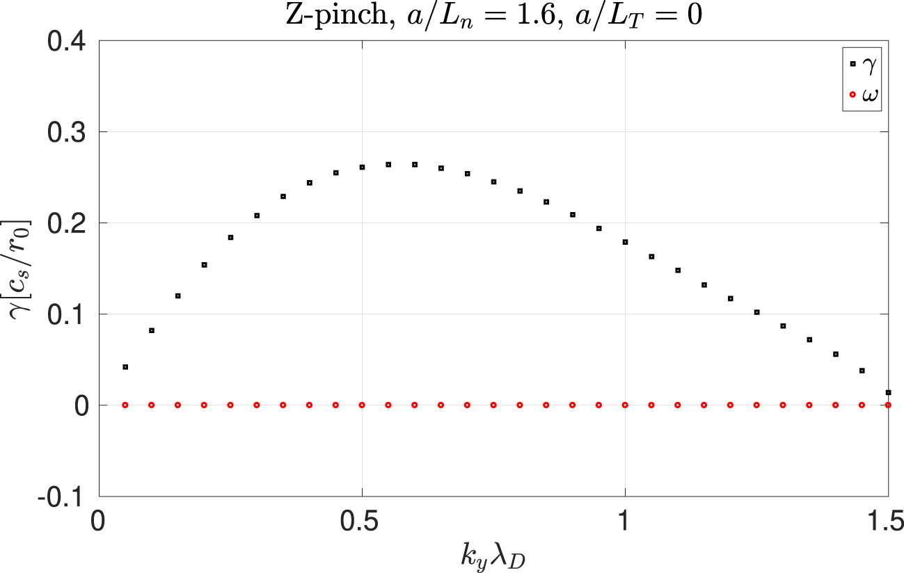
In figure 7 we show the results of scanning over the perpendicular wavenumber with FLR effects neglected. The instability is suppressed for large values of  $k_{\bot }\unicode[STIX]{x1D706}_{D}$ even in the absence of FLR effects.
Growth rate and frequency of the entropy mode as a function of  $k_{y}\unicode[STIX]{x1D706}_{D}$ for a large Debye length plasma in the Z-pinch. Note that, in agreement with theoretical prediction, the instability is quashed for large values of the Debye length.
This result is further emphasised in figure 8 where we see that including a large Debye length has hugely increased the region of absolute linear stability for the short-wavelength modes. This is a regime which is inaccessible to fusion experiments. The very low density expected in electron–positron plasmas should cause the Debye length to be large enough to stabilise short-wavelength modes (Helander Reference Helander2014). It should be pointed out that increasing the Debye length shifts the stability lines present in the previous figures in the positive gradient directions as can be seen from (6.3) and (6.4). That is, the stability map shown in figure 8(b) could be made to look identical to that in panel (a) by scanning over larger values of the density and temperature gradients.
Stability diagram for several values of  $k_{y}\unicode[STIX]{x1D706}_{D}$ for a large Debye length plasma in the Z-pinch. The colour of the density plot corresponds to numerically obtained growth rate this time calculated using GENE simulations. The region of stability is white and bordered by a solid black contour.

There is a simple analytical reason for these observations, pertaining to the threshold for both the entropy mode and the interchange mode. Namely, these results follow immediately from (6.5) which predicts the threshold for which the interchange mode becomes Landau damped. In this regime, larger density and temperature gradients would be required to drive instability in the system. Indeed, it seems that the electron–positron plasmas of experimental interest certainly will enjoy the remarkable stability properties predicted in simpler geometries.
8 Outlook and conclusions
In this work, we have implemented a dipole geometry, for use with the gyrokinetic code GENE, to study linear electrostatic gyrokinetic modes in a pair plasma confined in a magnetic dipole. We have studied both an experimentally relevant flux tube representative of a true experimental dipole system such as is planned in upcoming pair-plasma experiments, and also the near-ring limit of a Z-pinch for benchmarking purposes. Similar to existing studies in electron–ion plasmas, we find that the general features of electrostatic drift modes in dipole configuration pair plasmas are similar to those found in Z-pinch pair plasmas, with numerical differences originating in the choice of normalisation, i.e. we find that both interchange and entropy modes are present in the system.
We were able to use Z-pinch geometry in order to reproduce and validate existing analytic theory on the stability of electron–positron plasmas for different temperature and density gradients. This feature is in essence what will guide the next steps in this research. Namely, the analytic theory also predicts inward particle transport Helander & Connor (Reference Helander and Connor2016) in such systems and we aim to validate this with nonlinear simulations of electron–positron plasmas, using a global gyrokinetic code, in the immediate future.
Of critical importance to the upcoming experiments, we have shown that the remarkable stability properties thus far predicted and investigated for approximate geometries do indeed hold true in the more complicated geometry of the magnetic field due to a current-carrying circular coil. We have also been able to confirm that the large Debye length expected in such plasmas due to the very low densities available, should indeed be sufficient to stabilise short-wavelength modes and that, crucially, the first terrestrial electron–positron plasmas ought to enjoy splendid confinement.
Acknowledgements
We acknowledge T. S. Pedersen and the PAX/APEX experiment team for their interest in our work.
Appendix A. Magnetic field derivatives in polar coordinates
In the following appendices, we describe how the various different metric quantities required by GENE are calculated using the input values given in table 1.
In cylindrical coordinates, one can write
 $$\begin{eqnarray}\unicode[STIX]{x1D713}(r,z)=\frac{\unicode[STIX]{x1D707}_{0}I}{2\unicode[STIX]{x03C0}}\sqrt{(r_{0}+r)^{2}+z^{2}}\left[\frac{r_{0}^{2}+r^{2}+z^{2}}{(r_{0}+r)^{2}+z^{2}}K(\unicode[STIX]{x1D705})-E(\unicode[STIX]{x1D705})\right],\end{eqnarray}$$
 $$\begin{eqnarray}\unicode[STIX]{x1D705}=\sqrt{\frac{4r_{0}r}{(r_{0}+r)^{2}+z^{2}}},\quad \boldsymbol{B}(r,z)=\unicode[STIX]{x1D735}\unicode[STIX]{x1D713}(r,z)\times \unicode[STIX]{x1D735}\unicode[STIX]{x1D711},\quad \unicode[STIX]{x1D735}\unicode[STIX]{x1D711}=\frac{\boldsymbol{e}_{\unicode[STIX]{x1D711}}}{r},\end{eqnarray}$$
where we have defined
 $$\begin{eqnarray}\unicode[STIX]{x1D6FC}^{2}=(r_{0}-r)^{2}+z^{2},\quad \unicode[STIX]{x1D6FD}^{2}=(r_{0}+r)^{2}+z^{2},\quad \unicode[STIX]{x1D705}^{2}=1-\unicode[STIX]{x1D6FC}^{2}/\unicode[STIX]{x1D6FD}^{2},\quad C=\frac{\unicode[STIX]{x1D707}_{0}I}{\unicode[STIX]{x03C0}}.\end{eqnarray}$$
Following Simpson et al. (Reference Simpson, Lane, Immer and Youngquist2001), one can then write down the magnetic field components
 $$\begin{eqnarray}\displaystyle & \displaystyle B_{r}=\frac{Cz}{2\unicode[STIX]{x1D6FC}^{2}\unicode[STIX]{x1D6FD}r}[(r_{0}^{2}+r^{2}+z^{2})E(\unicode[STIX]{x1D705}^{2})-\unicode[STIX]{x1D6FC}^{2}K(\unicode[STIX]{x1D705}^{2})], & \displaystyle\end{eqnarray}$$
 $$\begin{eqnarray}\displaystyle & \displaystyle B_{z}=\frac{C}{2\unicode[STIX]{x1D6FC}^{2}\unicode[STIX]{x1D6FD}}[(r_{0}^{2}-r^{2}-z^{2})E(\unicode[STIX]{x1D705}^{2})+\unicode[STIX]{x1D6FC}^{2}K(\unicode[STIX]{x1D705}^{2})], & \displaystyle\end{eqnarray}$$
and the derivatives of the magnetic field
 $$\begin{eqnarray}\displaystyle \frac{\unicode[STIX]{x2202}B_{r}}{\unicode[STIX]{x2202}r} & = & \displaystyle -\frac{Cz}{2r^{2}\unicode[STIX]{x1D6FC}^{4}\unicode[STIX]{x1D6FD}^{3}}\{\! [r_{0}^{6}+(r^{2}+z^{2})^{2}(2r^{2}+z^{2})+r_{0}^{4}(3z^{2}-8r^{2})\nonumber\\ \displaystyle & & \displaystyle +\,r_{0}^{2}(5r^{4}-4r^{2}z^{2}+3z^{4})]E(\unicode[STIX]{x1D705}^{2})\nonumber\\ \displaystyle & & \displaystyle -\,\unicode[STIX]{x1D6FC}^{2}[r_{0}^{4}-3r_{0}^{2}r^{2}+2r^{4}+(2r_{0}^{2}+3r^{2})z^{2}+z^{4}]K(\unicode[STIX]{x1D705}^{2})\!\},\end{eqnarray}$$
 $$\begin{eqnarray}\displaystyle \frac{\unicode[STIX]{x2202}B_{r}}{\unicode[STIX]{x2202}z} & = & \displaystyle \frac{C}{2r\unicode[STIX]{x1D6FC}^{4}\unicode[STIX]{x1D6FD}^{3}}\{[(r_{0}^{2}+r^{2})(z^{4}+(r_{0}^{2}-r^{2})^{2})+2z^{2}(r_{0}^{4}-6r_{0}^{2}r^{2}+r^{4})]E(\unicode[STIX]{x1D705}^{2})\nonumber\\ \displaystyle & & \displaystyle -\,\unicode[STIX]{x1D6FC}^{2}[(r_{0}^{2}-r^{2})^{2}+(r_{0}^{2}+r^{2})z^{2}]K(\unicode[STIX]{x1D705}^{2})\!\},\end{eqnarray}$$
 $$\begin{eqnarray}\displaystyle & \displaystyle \frac{\unicode[STIX]{x2202}B_{z}}{\unicode[STIX]{x2202}z}=\frac{Cz}{2\unicode[STIX]{x1D6FC}^{4}\unicode[STIX]{x1D6FD}^{3}}\{[6r_{0}^{2}(r^{2}-z^{2})-7r_{0}^{4}+(r^{2}+z^{2})^{2}]E(\unicode[STIX]{x1D705}^{2})+\unicode[STIX]{x1D6FC}^{2}[r_{0}^{2}-r^{2}-z^{2}]K(\unicode[STIX]{x1D705}^{2})\},\qquad & \displaystyle\end{eqnarray}$$
 $$\begin{eqnarray}\frac{\unicode[STIX]{x2202}B_{z}}{\unicode[STIX]{x2202}r}=\frac{\unicode[STIX]{x2202}B_{r}}{\unicode[STIX]{x2202}z},\quad B_{\unicode[STIX]{x1D711}}=0,\quad \frac{\unicode[STIX]{x2202}B_{r}}{\unicode[STIX]{x2202}\unicode[STIX]{x1D711}}=\frac{\unicode[STIX]{x2202}B_{z}}{\unicode[STIX]{x2202}\unicode[STIX]{x1D711}}=0.\end{eqnarray}$$
The derivatives of the magnetic flux can then be written as follows.
 $$\begin{eqnarray}\frac{\unicode[STIX]{x2202}\unicode[STIX]{x1D713}}{\unicode[STIX]{x2202}r}=rB_{z},\quad \frac{\unicode[STIX]{x2202}\unicode[STIX]{x1D713}}{\unicode[STIX]{x2202}z}=-rB_{r},\quad \frac{\unicode[STIX]{x2202}^{2}\unicode[STIX]{x1D713}}{\unicode[STIX]{x2202}r^{2}}=B_{z}+r\frac{\unicode[STIX]{x2202}B_{z}}{\unicode[STIX]{x2202}r},\quad \frac{\unicode[STIX]{x2202}^{2}\unicode[STIX]{x1D713}}{\unicode[STIX]{x2202}z^{2}}=-r\frac{\unicode[STIX]{x2202}B_{r}}{\unicode[STIX]{x2202}z}\end{eqnarray}$$
 $$\begin{eqnarray}\frac{\unicode[STIX]{x2202}^{2}\unicode[STIX]{x1D713}}{\unicode[STIX]{x2202}r\unicode[STIX]{x2202}z}=r\frac{\unicode[STIX]{x2202}B_{z}}{\unicode[STIX]{x2202}z}=-B_{r}-r\frac{\unicode[STIX]{x2202}B_{r}}{\unicode[STIX]{x2202}r},\quad \unicode[STIX]{x1D735}\boldsymbol{\cdot }\boldsymbol{B}=\frac{\unicode[STIX]{x2202}B_{r}}{\unicode[STIX]{x2202}r}+\frac{B_{r}}{r}+\frac{\unicode[STIX]{x2202}B_{z}}{\unicode[STIX]{x2202}z}.\end{eqnarray}$$
 Note that, taking into account  $\unicode[STIX]{x2202}B_{r}/\unicode[STIX]{x2202}z=\unicode[STIX]{x2202}B_{z}/\unicode[STIX]{x2202}r$ and using the definitions of the magnetic flux derivatives, one arrives at the Grad–Shafranov equation for the low-beta ( $p\approx 0$) dipole geometry ( $F=rB_{\unicode[STIX]{x1D711}}=0$).
 $$\begin{eqnarray}\unicode[STIX]{x1D6E5}^{\ast }\unicode[STIX]{x1D713}=\frac{\unicode[STIX]{x2202}^{2}\unicode[STIX]{x1D713}}{\unicode[STIX]{x2202}r^{2}}-\frac{1}{r}\frac{\unicode[STIX]{x2202}\unicode[STIX]{x1D713}}{\unicode[STIX]{x2202}r}+\frac{\unicode[STIX]{x2202}^{2}\unicode[STIX]{x1D713}}{\unicode[STIX]{x2202}z^{2}}=-\unicode[STIX]{x1D707}_{0}r^{2}\frac{\text{d}p}{\text{d}\unicode[STIX]{x1D713}}-\frac{1}{2}\frac{\text{d}F^{2}}{\text{d}\unicode[STIX]{x1D713}}=0\;\Leftrightarrow \;\frac{\unicode[STIX]{x2202}^{2}\unicode[STIX]{x1D713}}{\unicode[STIX]{x2202}r^{2}}+\frac{\unicode[STIX]{x2202}^{2}\unicode[STIX]{x1D713}}{\unicode[STIX]{x2202}z^{2}}=B_{z}.\end{eqnarray}$$
Note also the condition of no ambient current outside the current ring:
 $$\begin{eqnarray}\unicode[STIX]{x1D735}\times \boldsymbol{B}=0,\quad (\unicode[STIX]{x1D735}\times \boldsymbol{B})_{r}=0,\quad (\unicode[STIX]{x1D735}\times \boldsymbol{B})_{\unicode[STIX]{x1D711}}=\frac{\unicode[STIX]{x2202}B_{r}}{\unicode[STIX]{x2202}z}-\frac{\unicode[STIX]{x2202}B_{z}}{\unicode[STIX]{x2202}r},\quad (\unicode[STIX]{x1D735}\times \boldsymbol{B})_{z}=0.\end{eqnarray}$$
These derivatives are used in the calculation of the various metric quantities required by GENE, which are detailed in appendix B.
Appendix B. Metric coefficients in flux-tube coordinates
For use in GENE, various metric quantities need to be supplied through the geometry interface, GIST (Xanthopoulos et al. Reference Xanthopoulos, Cooper, Jenko, Turkin, Runov and Geiger2009). For the dipole system considered, we will find it useful to employ the magnetic coordinate system  $(s,\unicode[STIX]{x1D6FC},\unicode[STIX]{x1D703})$, defined below. These quantities are then given to GENE and transformed into the appropriate local coordinate system directly, to construct the computational domain. The elements required by GENE are
 $$\begin{eqnarray}\displaystyle & \displaystyle {\hat{g}}_{11}=\hat{\unicode[STIX]{x1D735}}s\boldsymbol{\cdot }\hat{\unicode[STIX]{x1D735}}s=\left(\frac{r_{\ast }}{\unicode[STIX]{x1D713}_{\text{min}}-\unicode[STIX]{x1D713}_{\text{max}}}\right)^{2}\unicode[STIX]{x1D735}\unicode[STIX]{x1D713}\boldsymbol{\cdot }\unicode[STIX]{x1D735}\unicode[STIX]{x1D713}=\frac{1}{(B_{\ast }r_{\ast })^{2}}\unicode[STIX]{x1D735}\unicode[STIX]{x1D713}\boldsymbol{\cdot }\unicode[STIX]{x1D735}\unicode[STIX]{x1D713}, & \displaystyle\end{eqnarray}$$
 $$\begin{eqnarray}\displaystyle & \displaystyle {\hat{g}}_{12}=\hat{\unicode[STIX]{x1D735}s}\boldsymbol{\cdot }\hat{\unicode[STIX]{x1D735}}\unicode[STIX]{x1D6FC}=0, & \displaystyle\end{eqnarray}$$
 $$\begin{eqnarray}\displaystyle & \displaystyle {\hat{g}}_{22}=\hat{\unicode[STIX]{x1D735}}\unicode[STIX]{x1D6FC}\boldsymbol{\cdot }\hat{\unicode[STIX]{x1D735}}\unicode[STIX]{x1D6FC}=r_{\ast }^{2}|\unicode[STIX]{x1D735}\unicode[STIX]{x1D711}|^{2}=\frac{r_{\ast }^{2}}{r^{2}}, & \displaystyle\end{eqnarray}$$
 $$\begin{eqnarray}\displaystyle & \displaystyle \hat{J}=[(\hat{\unicode[STIX]{x1D735}}s\times \hat{\unicode[STIX]{x1D735}}\unicode[STIX]{x1D6FC})\boldsymbol{\cdot }\hat{\unicode[STIX]{x1D735}}\unicode[STIX]{x1D703}]^{-1}=-\frac{B_{\ast }}{r_{\ast }}[(\unicode[STIX]{x1D735}\unicode[STIX]{x1D713}\times \unicode[STIX]{x1D735}\unicode[STIX]{x1D703})\boldsymbol{\cdot }\unicode[STIX]{x1D735}\unicode[STIX]{x1D711}]^{-1}, & \displaystyle\end{eqnarray}$$
 $$\begin{eqnarray}\hat{B}=\frac{B}{|B_{\ast }|},\quad \frac{\unicode[STIX]{x2202}\hat{B}}{\unicode[STIX]{x2202}\unicode[STIX]{x1D703}}=\frac{1}{B_{\ast }}\frac{\unicode[STIX]{x2202}B}{\unicode[STIX]{x2202}\unicode[STIX]{x1D703}},\end{eqnarray}$$
 $$\begin{eqnarray}\displaystyle & \displaystyle \hat{L}_{1}=\left(\boldsymbol{b}\times \frac{\hat{\unicode[STIX]{x1D735}}\hat{B}}{\hat{B}}\right)\boldsymbol{\cdot }\hat{\unicode[STIX]{x1D735}}s=0, & \displaystyle\end{eqnarray}$$
 $$\begin{eqnarray}\displaystyle & \displaystyle \hat{L}_{2}=\left(\boldsymbol{b}\times \frac{\hat{\unicode[STIX]{x1D735}}\hat{B}}{\hat{B}}\right)\boldsymbol{\cdot }\hat{\unicode[STIX]{x1D735}}\unicode[STIX]{x1D6FC}=-r_{\ast }^{2}\left(\boldsymbol{b}\times \frac{\unicode[STIX]{x1D735}B}{B}\right)\boldsymbol{\cdot }\unicode[STIX]{x1D735}\unicode[STIX]{x1D711}. & \displaystyle\end{eqnarray}$$
Again, in order to calculate these quantities one must calculate various derivatives.
Once again introducing  $r_{0}$ as the radius of the circular current loop creating the magnetic field, $I$ the current flowing in the loop, $\unicode[STIX]{x1D713}_{\text{max}}$ the poloidal magnetic flux at the inner boundary and $\unicode[STIX]{x1D713}_{\text{min}}$ the poloidal flux at the outer boundary of the domain considered. We choose the magnetic coordinates as follows:
 $$\begin{eqnarray}s=\frac{\unicode[STIX]{x1D713}-\unicode[STIX]{x1D713}_{\text{max}}}{\unicode[STIX]{x1D713}_{\text{min}}-\unicode[STIX]{x1D713}_{\text{max}}},\quad \unicode[STIX]{x1D703}=\frac{2\unicode[STIX]{x03C0}l}{L_{0}}-\unicode[STIX]{x03C0}.\end{eqnarray}$$
 For a dipole,  $\unicode[STIX]{x1D703}$ is the field-line following coordinate and $l$ parameterises the length along the field line. We have normalised the length to the properly chosen $r_{\ast }$ (e.g. $r_{\ast }=r_{0}$), and the magnetic field to $B_{\ast }$ given by
 $$\begin{eqnarray}\boldsymbol{B}=\unicode[STIX]{x1D735}\unicode[STIX]{x1D713}\times \unicode[STIX]{x1D735}\unicode[STIX]{x1D711}=-B_{\ast }\hat{\unicode[STIX]{x1D735}}s\times \hat{\unicode[STIX]{x1D735}}\unicode[STIX]{x1D711}=B_{\ast }\hat{\unicode[STIX]{x1D735}}s\times \hat{\unicode[STIX]{x1D735}}\unicode[STIX]{x1D6FC}\end{eqnarray}$$
 $$\begin{eqnarray}\hat{\unicode[STIX]{x1D735}}=r_{\ast }\unicode[STIX]{x1D735},\quad B_{\ast }=\frac{\unicode[STIX]{x1D713}_{\text{max}}-\unicode[STIX]{x1D713}_{\text{min}}}{r_{\ast }^{2}},\quad \unicode[STIX]{x1D6FC}=-\unicode[STIX]{x1D711}.\end{eqnarray}$$
 The derivative of the magnetic field strength along the field line,  $\unicode[STIX]{x2202}B/\unicode[STIX]{x2202}\unicode[STIX]{x1D703}$, is given by
 $$\begin{eqnarray}\left.\frac{\unicode[STIX]{x2202}B}{\unicode[STIX]{x2202}\unicode[STIX]{x1D703}}\right|_{\unicode[STIX]{x1D713}}=\frac{1}{B}\left(\left.B_{r}\frac{\unicode[STIX]{x2202}B_{r}}{\unicode[STIX]{x2202}\unicode[STIX]{x1D703}}\right|_{\unicode[STIX]{x1D713}}+\left.B_{z}\frac{\unicode[STIX]{x2202}B_{z}}{\unicode[STIX]{x2202}\unicode[STIX]{x1D703}}\right|_{\unicode[STIX]{x1D713}}\right).\end{eqnarray}$$
Hence,
 $$\begin{eqnarray}\left.\frac{\unicode[STIX]{x2202}B_{r}}{\unicode[STIX]{x2202}\unicode[STIX]{x1D703}}\right|_{\unicode[STIX]{x1D713}}=\left.\frac{\unicode[STIX]{x2202}B_{r}}{\unicode[STIX]{x2202}r}\right|_{z}\left.\frac{\unicode[STIX]{x2202}r}{\unicode[STIX]{x2202}\unicode[STIX]{x1D703}}\right|_{\unicode[STIX]{x1D713}}+\left.\frac{\unicode[STIX]{x2202}B_{r}}{\unicode[STIX]{x2202}z}\right|_{r}\left.\frac{\unicode[STIX]{x2202}z}{\unicode[STIX]{x2202}\unicode[STIX]{x1D703}}\right|_{\unicode[STIX]{x1D713}}.\end{eqnarray}$$
Similarly,
 $$\begin{eqnarray}\left.\frac{\unicode[STIX]{x2202}B_{z}}{\unicode[STIX]{x2202}\unicode[STIX]{x1D703}}\right|_{\unicode[STIX]{x1D713}}=\left.\frac{\unicode[STIX]{x2202}B_{z}}{\unicode[STIX]{x2202}r}\right|_{z}\left.\frac{\unicode[STIX]{x2202}r}{\unicode[STIX]{x2202}\unicode[STIX]{x1D703}}\right|_{\unicode[STIX]{x1D713}}+\left.\frac{\unicode[STIX]{x2202}B_{z}}{\unicode[STIX]{x2202}z}\right|_{r}\left.\frac{\unicode[STIX]{x2202}z}{\unicode[STIX]{x2202}\unicode[STIX]{x1D703}}\right|_{\unicode[STIX]{x1D713}}.\end{eqnarray}$$
These quantities are calculated using a field-line tracing routine outlined below. The details of how this coordinate system is mapped to the GENE coordinate system can be found in Xanthopoulos et al. (Reference Xanthopoulos, Cooper, Jenko, Turkin, Runov and Geiger2009).
The field-line tracing is defined by the equations
 $$\begin{eqnarray}\frac{\text{d}r}{\text{d}l}=\frac{B_{r}(r,z)}{B(r,z)}=b_{r},\quad \frac{\text{d}z}{\text{d}l}=\frac{B_{z}(r,z)}{B(r,z)}=b_{z},\quad r(0)=r_{c},\quad z(0)=0.\end{eqnarray}$$
 Here,  $l$ is the length measured along the field line and $r_{c}$ defines the flux surface. Note that by definition
 $$\begin{eqnarray}\displaystyle & \displaystyle \frac{\unicode[STIX]{x2202}\unicode[STIX]{x1D703}}{\unicode[STIX]{x2202}l}=\frac{2\unicode[STIX]{x03C0}}{L_{0}}, & \displaystyle\end{eqnarray}$$
 $$\begin{eqnarray}\displaystyle & \displaystyle \frac{\unicode[STIX]{x2202}l}{\unicode[STIX]{x2202}\unicode[STIX]{x1D703}}=\frac{L_{0}}{2\unicode[STIX]{x03C0}}. & \displaystyle\end{eqnarray}$$
 Here,  $L_{0}$ is the length of the closed field line. Using the properties
 $$\begin{eqnarray}\boldsymbol{r}_{,l}\boldsymbol{\cdot }\unicode[STIX]{x1D735}l=1,\quad |\unicode[STIX]{x1D735}l|=1,\end{eqnarray}$$
we arrive at the equations
 $$\begin{eqnarray}\frac{\text{d}r}{\text{d}l}\frac{\unicode[STIX]{x2202}l}{\unicode[STIX]{x2202}r}+\frac{\text{d}z}{\text{d}l}\frac{\unicode[STIX]{x2202}l}{\unicode[STIX]{x2202}z}=1,\quad \left(\frac{\unicode[STIX]{x2202}l}{\unicode[STIX]{x2202}r}\right)^{2}+\left(\frac{\unicode[STIX]{x2202}l}{\unicode[STIX]{x2202}z}\right)^{2}=1.\end{eqnarray}$$
These can be rewritten as
 $$\begin{eqnarray}b_{r}\frac{\unicode[STIX]{x2202}l}{\unicode[STIX]{x2202}r}+b_{z}\frac{\unicode[STIX]{x2202}l}{\unicode[STIX]{x2202}z}=1,\quad \left(\frac{\unicode[STIX]{x2202}l}{\unicode[STIX]{x2202}r}\right)^{2}+\left(\frac{\unicode[STIX]{x2202}l}{\unicode[STIX]{x2202}z}\right)^{2}=1,\end{eqnarray}$$
 and solved, taking into account that  $b_{r}^{2}+b_{z}^{2}=1$, with the result
 $$\begin{eqnarray}\frac{\unicode[STIX]{x2202}l}{\unicode[STIX]{x2202}r}=b_{r},\quad \frac{\unicode[STIX]{x2202}l}{\unicode[STIX]{x2202}z}=b_{z}.\end{eqnarray}$$
Finally, in our coordinates we obtain
 $$\begin{eqnarray}\frac{\text{d}r}{\text{d}\unicode[STIX]{x1D703}}=\frac{L_{0}}{2\unicode[STIX]{x03C0}}b_{r},\quad \frac{\text{d}z}{\text{d}\unicode[STIX]{x1D703}}=\frac{L_{0}}{2\unicode[STIX]{x03C0}}b_{z},\end{eqnarray}$$
 $$\begin{eqnarray}\frac{\unicode[STIX]{x2202}\unicode[STIX]{x1D703}}{\unicode[STIX]{x2202}r}=\frac{2\unicode[STIX]{x03C0}}{L_{0}}b_{r},\quad \frac{\unicode[STIX]{x2202}\unicode[STIX]{x1D703}}{\unicode[STIX]{x2202}z}=\frac{2\unicode[STIX]{x03C0}}{L_{0}}b_{z}.\end{eqnarray}$$
Note further geometric properties
 $$\begin{eqnarray}\boldsymbol{r}_{,l}\boldsymbol{\cdot }\unicode[STIX]{x1D735}\unicode[STIX]{x1D713}=0,\quad \unicode[STIX]{x1D735}l\boldsymbol{\cdot }\boldsymbol{r}_{,\unicode[STIX]{x1D713}}=0,\quad \boldsymbol{r}_{,\unicode[STIX]{x1D713}}\boldsymbol{\cdot }\unicode[STIX]{x1D735}\unicode[STIX]{x1D713}=1,\end{eqnarray}$$
which can be proven taking into account that for the dipole magnetic field
 $$\begin{eqnarray}\frac{\unicode[STIX]{x2202}\unicode[STIX]{x1D713}}{\unicode[STIX]{x2202}r}=rB_{z},\quad \frac{\unicode[STIX]{x2202}\unicode[STIX]{x1D713}}{\unicode[STIX]{x2202}z}=-rB_{r},\quad \unicode[STIX]{x1D735}\unicode[STIX]{x1D713}=Br(b_{z}\boldsymbol{e}_{r}-b_{r}\boldsymbol{e}_{z}),\end{eqnarray}$$
and the geometric relations
 $$\begin{eqnarray}\boldsymbol{r}_{,\unicode[STIX]{x1D713}}=\sqrt{g}\;\unicode[STIX]{x1D735}\unicode[STIX]{x1D701}\times \unicode[STIX]{x1D735}\unicode[STIX]{x1D703},\quad \frac{1}{\sqrt{g}}=(\unicode[STIX]{x1D735}\unicode[STIX]{x1D713}\times \unicode[STIX]{x1D735}\unicode[STIX]{x1D701})\boldsymbol{\cdot }\unicode[STIX]{x1D735}\unicode[STIX]{x1D703}.\end{eqnarray}$$
 Note the coordinate system orientation  $(\unicode[STIX]{x1D713},\unicode[STIX]{x1D701},\unicode[STIX]{x1D703})$ which is consistent with GENE. Using cylindrical coordinates $(r,\unicode[STIX]{x1D701},z)$ with the orientation corresponding to the basis vectors $\boldsymbol{e}_{\unicode[STIX]{x1D701}}=\boldsymbol{e}_{z}\times \boldsymbol{e}_{r}$ in dipole magnetic field, we can write
 $$\begin{eqnarray}\frac{1}{\sqrt{g}}=\frac{2\unicode[STIX]{x03C0}B}{L_{0}},\quad \unicode[STIX]{x1D735}\unicode[STIX]{x1D701}\times \unicode[STIX]{x1D735}\unicode[STIX]{x1D703}=\frac{2\unicode[STIX]{x03C0}}{L_{0}r}(b_{z}\boldsymbol{e}_{r}-b_{r}\boldsymbol{e}_{z}),\quad \boldsymbol{r}_{,\unicode[STIX]{x1D713}}=\frac{b_{z}\boldsymbol{e}_{r}-b_{r}\boldsymbol{e}_{z}}{Br}.\end{eqnarray}$$
 Here again, is obvious that  $\boldsymbol{r}_{,\unicode[STIX]{x1D713}}\boldsymbol{\cdot }\unicode[STIX]{x1D735}\unicode[STIX]{x1D713}=1$. For the normalisation, one can use
 $$\begin{eqnarray}r_{\star }=\frac{L_{0}}{2\unicode[STIX]{x03C0}},\quad B_{\star }=B(l=L_{0}/2).\end{eqnarray}$$


 Open access