


1. Introduction
In its most recent edition, the Intergovernmental Panel on Climate Change (IPCC) finds that global temperatures have been steadily rising, with more noticeable shifts observed in recent decades (IPCC, Reference Masson-Delmotte, Zhai, Pirani, SL, Péan, Berger, Caud, Chen, Goldfarb, Gomis, Huang, Leitzell, Lonnoy, Matthews, Maycock, Waterfield, Yelekçi, Yu and Zhou2021). The report highlights that the global temperature was 1.09°C warmer in the second decade of the twenty-first century than in the period 1850–1900. Not only are temperatures rising, but they are doing so at an accelerating rate. Consistent with this, extreme climate phenomena like heatwaves and droughts have become more common as a result of these temperature increases. This trend is expected to intensify in the upcoming years under all climate change scenarios (IPCC, Reference Masson-Delmotte, Zhai, Pirani, SL, Péan, Berger, Caud, Chen, Goldfarb, Gomis, Huang, Leitzell, Lonnoy, Matthews, Maycock, Waterfield, Yelekçi, Yu and Zhou2021; Trisos et al., Reference Trisos, Adelekan, Totin, Ayanlade, Efitre, Gemeda, Kalaba, Lennard, Masao, Mgaya, Ngaruiya, Olago, Simpson, Zakieldeen, Pörtner, Roberts, Tignor, Poloczanska, Mintenbeck, Alegría, Craig, Langsdorf, Löschke, Möller, Okem and Rama2022). In recent decades, Africa’s climate has warmed faster than the worldwide average. There are noticeably more warm nights and warm days, along with an increase in the region’s annual maximum and minimum temperatures (IPCC, Reference Masson-Delmotte, Zhai, Pirani, SL, Péan, Berger, Caud, Chen, Goldfarb, Gomis, Huang, Leitzell, Lonnoy, Matthews, Maycock, Waterfield, Yelekçi, Yu and Zhou2021). Due to its poor institutional capacity to adjust to climate fluctuation, and the predominance of rain-fed agriculture on the continent, Africa is considered to be the continent most vulnerable to climate change (Dell et al., Reference Dell, Jones and Olken2012; Kjellstrom et al., Reference Kjellstrom, Briggs, Freyberg, Lemke, Otto and Hyatt2016; IPCC, Reference Masson-Delmotte, Zhai, Pirani, SL, Péan, Berger, Caud, Chen, Goldfarb, Gomis, Huang, Leitzell, Lonnoy, Matthews, Maycock, Waterfield, Yelekçi, Yu and Zhou2021).
Ethiopia’s altitude ranges from 125 meters below sea level to 4,620 meters above sea level. Hence, the climate varies greatly – from hot and arid in the lowlands to cool and temperate in the highlands. The mean annual temperature has increased by 1.3°C since 1960, an average rate of 0.28°C per decade. This decadal increment is above the global mean value of 0.2°C (Zegeye, Reference Zegeye2018). Daily temperature observations show that both hot days and hot nights are increasing in frequency (Addisu et al., Reference Addisu, Gebreselassie, Fissha and Gedif2015). The nation frequently experiences droughts, the most recent of which occurred in 2024, which has imposed significant costs on both life and property. Of greater concern is that the nation is projected to experience higher temperatures in the coming decades under every possible climate scenario (Simane et al., Reference Simane, Zaitchik and Foltz2016).
In light of rising global temperatures, Dell et al. (Reference Dell, Jones and Olken2014) contend that anticipating the expected consequences of climate change on a range of outcomes is critical for the estimation of the climate damage function. Moreover, a thorough grasp of these consequences is required for the effective design of economic policies and institutions that increase resilience to climate shocks. Therefore, in this paper, we investigate whether temperature shocks affect the saving behaviour of rural households in Ethiopia. Apart from the significant research gap that links the effects of climate change to financial outcomes (Dell et al., Reference Dell, Jones and Olken2014), the analysis of household savings deserves special consideration because of the critical role of savings in rural livelihoods. In rural Ethiopia, credit and insurance markets are imperfect and limited, which forces households to rely primarily on their own savings to smooth consumption in the face of both idiosyncratic and covariate shocks (Amha and Alemu, Reference Amha and Alemu2014; Elias et al., Reference Elias, Beshir and Mehare2022). Beyond consumption smoothing, household savings are central to financing productive inputs such as improved seeds, fertilizer and irrigation (Avdeenko et al., Reference Avdeenko, Bohne and Frolich2019; Elias et al., Reference Elias, Beshir and Mehare2022). By easing liquidity constraints, savings also enhance participation in off-farm activities. Moreover, savings are crucial to households’ long-term welfare by enabling sustained investment in both physical and human capital (Dercon, Reference Dercon, Mody and Pattillo2004; Avdeenko et al., Reference Avdeenko, Bohne and Frolich2019).
Although the importance of savings for rural households is well documented, savings mobilizations among rural households in Ethiopia are low (Amha and Alemu, Reference Amha and Alemu2014; World Bank Group, 2018). In many low-income countries, significant challenges persist that constrain households’ ability to accumulate savings. In particular, the high volatility of agricultural income (Dercon, Reference Dercon, Mody and Pattillo2004; Karlan and Morduch, Reference Karlan, Morduch, Rodrik and Rosenzweig2010; Amha and Peck, Reference Amha and Peck2019), low levels of agricultural production and productivity (Amha and Peck, Reference Amha and Peck2019) and limited access to formal financial institutions (FFIs) and lack of diversified financial products (Banerjee and Duflo, Reference Banerjee and Duflo2007; Beck et al., Reference Beck, Demirguc-Kunt and Peria2007; Karlan et al., Reference Karlan, Ratan and Zinman2014) either restrict savings accumulation or lead to their depletion. In addition, behavioural factors – such as present bias, self-control problems and risk preferences – pose further obstacles to savings mobilization (Karlan and Morduch, Reference Karlan, Morduch, Rodrik and Rosenzweig2010; Falk et al., Reference Falk, Becker, Dohmen, Enke, Huffman and Sunde2018; Churchill et al., Reference Churchill, Smyth, Trinh and Yew2022). Building on this behavioural perspective, this paper further examines whether the impact of climate change on households’ saving behaviour in rural Ethiopia is mediated by time and risk preferences. These preferences are known to shape individual saving decisions and may themselves be influenced by climatic conditions (Callen, Reference Callen2015; Cassar et al., Reference Cassar, Healy and Von Kessler2017; Churchill et al., Reference Churchill, Smyth, Trinh and Yew2022). This approach enables us to derive policy-relevant insights for the design of saving products that are better aligned with heterogeneous household preferences in the presence of increasing climate risks.
Our study follows on from the work of Churchill et al. (Reference Churchill, Smyth, Trinh and Yew2022, Reference Churchill, Trinh and Danquah2023), who studied the impact of temperature changes on household saving behaviour in Australia and Vietnam, respectively. More specifically, Churchill et al. (Reference Churchill, Smyth, Trinh and Yew2022) found that an increase in average temperature of 1 standard deviation is associated with a 4.3 per cent increase in net worth and a 12.8 per cent increase in savings among Australian households. Their analysis also suggested that time preferences mediate the relationship between temperature shocks and savings, but that risk preferences do not. In Vietnam, the direction of the relationship is reversed: 1 additional day with an average temperature greater than 30°C relative to the number of days in the 18–22°C range is associated with a 6.3 per cent decrease in household savings. Total agricultural production and rice production are the mechanisms through which temperature shocks influenced household savings (Churchill et al., Reference Churchill, Trinh and Danquah2023).
In addition to the policy relevance discussed above, our study contributes to the literature on this relatively underexplored area in the following aspects. First, unlike the studies done in Australia and Vietnam, our study focuses on rural households where the primary occupation – rain-fed farmingFootnote 1 – is heavily dependent on the climate. The effects are particularly important to quantify, because they are accentuated by institutions that are less well-equipped to manage climate change. Second, while earlier empirical works in Ethiopia on climate shocks have emphasized income-related impacts (e.g., Dercon, Reference Dercon, Mody and Pattillo2004; Demeke et al., Reference Demeke, Keil and Zeller2011; Hill and Porter, Reference Hill and Porter2017; Gao and Mills, Reference Gao and Mills2018; Terefe et al., Reference Terefe, Aredo, Workagegnehu and Tesfaye2024), a growing body of literature also documents important non-income behavioural responses. For instance, Fentie and Beyene (Reference Fentie and Beyene2019), Ahmed et al. (Reference Ahmed, Haji, Jaleta and Jemal2024) and Sinore and Wang (Reference Sinore and Wang2024) demonstrate that rural households adjust agricultural practices in response to climate variability, including crop choice, input use (such as fertilizer and improved seeds) and diversification strategies as risk-management mechanisms. Collectively, this body of work underscores that household responses to climate shocks extend beyond income effects and operate through multiple behavioural channels. Building on this literature, our study contributes by examining a relatively less explored dimension – household saving behaviour – and its linkage to temperature shocks through time and risk preferences. In light of this, we also compare the role of behavioural mediators (risk and time preferences) with an economic mediator (labour productivity) to assess the former’s relative significance in mediating the impact of temperature shock on households’ saving behaviour.
To shed light on these and related issues, we use two waves of household survey data, and temperature data extracted from Climate Engine/Terra Climate based on geo-references of households. Our results indicate that deviations in current temperature from the long-run mean – measured as standardized anomalies – significantly reduce the likelihood of savings among rural households. This result is robust with respect to alternative measures of saving behaviour, temperature anomalies and estimation techniques. Our results also indicate that neither adaptation to temperature shocks nor the intensification of such shocks has statistically significant long-term effects. However, this finding should be interpreted cautiously, as our analysis is based on only two waves of survey data, which constrains the ability to capture longer-term dynamics. The mediation analysis further reveals that both time and risk preferences channel part of the impact of temperature shocks on households’ saving behaviour, confirming their role as mediating mechanisms. According to our heterogeneity analysis, differentiating households based on their level of poverty, credit access and the types of shocks they experience reveals significant disparities. Households that are poor, without access to credit from FFIs, and that experience positive shocks (i.e., actual records above their long-run mean temperatures), are more severely affected by temperature shocks in terms of their likelihood of saving.
Overall, our findings demonstrate how important it is to consider financial consequences, such as household savings, when estimating the damage cost due to climate change. Our findings also show that a disproportionate amount of the negative consequences of temperature shocks fall on poor households and those without access to credit, underscoring the need for focused policy measures. Furthermore, the development of commitment-based saving instruments, such as saving mechanisms with automatic deductions at harvest time, is necessary to preserve long-term wellbeing, according to our findings that temperature shocks increase household impatience and risk-taking inclinations.
The remainder of this paper is organized as follows. In Section 2, we present the conceptual framework. A description of the data and summary statistics follows in Section 3. The empirical model specification and estimation issues are presented in Section 4. We present results and discussion in Section 5, after which we conclude in Section 6.
2. Conceptual framework: the linkage of temperature changes, risk and time preferences, and household saving
The brain’s chemistry, electrical properties and function are all temperature-sensitive (Hocking et al., Reference Hocking, Silberstein, Lau, Stough and Roberts2001). Moreover, exposure to heat has been shown to diminish attention, memory, information retention and processing and the performance of psycho-perceptual tasks (Hocking et al., Reference Hocking, Silberstein, Lau, Stough and Roberts2001; Minor et al., Reference Minor, Bjerre-Nielsen, Jonasdottir, Lehmann and Obradovich2020). Recent researches have attributed these results partly to heat-induced distributions in mood, sleep and cognition (Minor et al., Reference Minor, Bjerre-Nielsen, Jonasdottir, Lehmann and Obradovich2020; Almas et al., Reference Almas, Auffhammer, Bold, Bolliger, Dembo, Hsiang, Kitamura, Miguel and Pickmans2025). These channels are important from an economic perspective since these factors are associated with decision-making and the formation of economic preferences (Benjamin et al., Reference Benjamin, Brown and Shapiro2013; Carias et al., Reference Carias, Johnston, Knott and Sweeney2021). Inspired by these insights, we develop a theoretical framework/model that shows how temperature shocks can affect households’ saving behaviour through effects on risk and intertemporal preferences. The details are presented in Section A of the online appendix.
In sum, the conceptual model and related empirics show that the effect of temperature shocks on households’ savings through time and risk preferences is inconclusive. These lacks of consensus in the literature motivate us to assess which of the findings hold in our case study. Moreover, Dell et al. (Reference Dell, Jones and Olken2014) argue that heterogeneity of climate impacts also arises from the nature of climatic shocks themselves (i.e., positive and negative temperature shocks), household attributes/status (e.g., poverty status of households) and their financial environment such as availability of credit and insurance markets and institutions. This highlights the significance of a more detailed analysis that takes into account these heterogeneity characteristics when evaluating how temperature shocks affect the saving behaviour of households.
3. Data and descriptive statistics
We rely on two waves of panel household survey data. The first round of data was collected by the Association of Ethiopian Microfinance Institutions in 2014. The survey questions address a wide range of socio-economic and financial issues. The second round was collected in 2018 by the Policy Studies and Research Institute, which was subsequently merged into the Policy Studies Institute. All the households surveyed in the first round were included in the second round, and the same questionnaire was used in both rounds.Footnote 2 Both surveys were conducted during the months of November and December of the respective years, and samples were drawn from the major regions of the country (i.e., Tigray, Amhara, Oromia, Afar, Somalia and SNNPR (Southern Nations, Nationalities, and Peoples’ Region)). Sample districts (woredas) were selected from each region, and respondents were drawn at random from the selected woredas, with sufficient representation from each district and region. To ensure a fair representation of samples from different areas, samples were taken from each of the various agroecologies of the country (i.e., Dega, Woina Dega, Kola and Berha). After cleaning the data thoroughly, we obtained a balanced panel of 1,436 rural households (i.e., a total sample of 2,872 = 1,436 × 2 rounds). The attrition rate was low (4.33 per cent) for the entire five years, indicating a dropout rate of less than 1 per cent p.a.Footnote 3
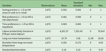
In Table 1, we present our main variables of interest with their respective descriptive values. Accordingly, we have a household’s saving status, which is a dummy variable with a value equal to 1 if a household practised savings either in cash or in-kindFootnote 4 in the year before the survey. The pooled data show that 59 per cent of rural households practise saving.
Variable descriptions and summary statistics

Table 1 Long description
Summary statistics are reported for seven household and climate variables, each based on 2,872 observations, including means, standard deviations, and minimum and maximum values. Three binary indicators show that 0.591 of households report saving in cash or in kind, 0.461 are classified as risk takers, and 0.685 are classified as impatient, making impatience the most prevalent of the three. Labor productivity, measured as income in Ethiopian Birr per active labor, averages 4,201.37 with a large spread of 7,291.43 and ranges from 0 to 70,914, indicating substantial variation and likely outliers. Long run mean temperature averages 19.79 with a standard deviation of 3.56, spanning 11.98 to 28.42. Deviation from the long run mean temperature averages 0.281 with a standard deviation of 0.172 and ranges from 0 to 0.63. A final row labeled standardized deviations has a mean of 0.18, a standard deviation of 0.10, and ranges from 0 to 0.43; the label is ambiguous without additional context, so interpretation should be cautious.
HH, household; ETB, Ethiopian birr (the local currency).
Source: Authors’ own computation, 2025.
As far as our mediator variables are concerned, households were asked to make a hypothetical choice between a normal interest-bearing savings product (i.e., paying fixed interest as a reward for deposits) and deposits where the rewards are determined by means of a lottery (i.e., an individual receives positive returns on deposits only if he/she wins the lottery). We label those who prefer deposits with the higher variance lottery-based rewards as ‘risk-takers’, since they are willing to forgo the stability of the set interest rewards paid on normal saving products. Theoretically, this classification is based on the expected utility theory of Von Neumann and Morgenstern (Reference Von Neumann and Morgenstern1953). Moreover, in its general essence, our measurement has bases in Holt and Laury (Reference Holt and Laury2002), Falk et al. (Reference Falk, Becker, Dohmen, Enke, Huffman and Sunde2018), Carias et al. (Reference Carias, Johnston, Knott and Sweeney2021) and Almas et al. (Reference Almas, Auffhammer, Bold, Bolliger, Dembo, Hsiang, Kitamura, Miguel and Pickmans2025), in which households are supposed to choose between a certain pay-off/safer options and risky options/lotteries.
Using this criterion, 46 per cent of households were classified as risk-takers, whereas the remaining are non-risk-takers. In order to determine inter-temporal preferences, we anchor on the increase in deposit interest rates (i.e., paid annually) that households demand in order to increase their savings.Footnote 5 Households with a bias towards the present have higher discount rates (Falk et al., Reference Falk, Becker, Dohmen, Enke, Huffman and Sunde2018; Carias et al., Reference Carias, Johnston, Knott and Sweeney2021), and require a larger increase in current deposit rates to defer their consumption from present to future. However, for more patient households, a more modest increase in the deposit rate results in higher savings. This question is framed in such a way that those households that decide to boost savings at lower rates are not offered options at higher rates. On this basis, 68.5 per cent of households are deemed as impatient, demanding a minimum 10 per cent increase in the deposit rate in order to increase their savings from the existing amount (Table 1).
Although the measurement of the mediator variables, namely risk and time preferences, follows established empirical approaches based on hypothetical choice scenarios, such measures may not fully capture the complexity and context-specific nature of underlying economic preferences. In particular, responses may be affected by framing effects, less precise domains or the hypothetical nature of the elicitation tasks. Consequently, the possibility of measurement error cannot be ruled out, and the interpretation of risk and time preferences as mediating mechanisms should therefore be viewed as suggestive rather than definitive.
We combine the panel household surveys with historical time-series temperature data to evaluate how temperature changes affect the saving habits of rural households. More precisely, geo-references – that is, longitude and latitude coordinates recorded during field surveys – help to locate households and extract monthly temperature records from the Terra Climate dataset using the climate engine website (ClimateEngine.org). More specifically, we extract temperature data for each enumeration area (EA), under the assumption that temperature does not vary significantly among households within the same EA. For consistency, monthly minimum and maximum temperatures were obtained over a 30-year period, corresponding to the intervals between survey waves (1985–2014 for the 2014 survey and 1989–2018 for the 2018 survey). A 30-year reference period was selected as it is sufficiently long to minimize sensitivity to short-term anomalies, while not so long as to misrepresent recent local climate shocks (Salazar-Espinoza et al., Reference Salazar-Espinoza, Jones and Tarp2015). This approach facilitates the high-precision identification of spatially and temporally comparable shocks (Tambet and Stopnitzky, Reference Tambet and Stopnitzky2021). Monthly temperature data from Terra Climate are available in the form of maximum and minimum records. Using this data, we follow Auffhammer et al. (Reference Auffhammer, Hsiang, Schlenker and Sobel2013), who assert that the mean temperature for a given month can be calculated by averaging the minimum and maximum monthly temperatures.
As reported in Table 1, the long-run mean temperature is 19.8°C. As noted above, we have surveys in the years 2014 and 2018 that contain information on the saving behaviour of households for the entire year. So as to capture the impact of temperature shocks on households’ saving behaviour in the survey years, standardized anomalies – which are calculated by dividing the difference between the actual temperature of a given EA in year t (i.e., 2014 or 2018) and the corresponding 30-year long-term average by the standard deviation (Dell et al., Reference Dell, Jones and Olken2014) – are used to quantify temperature shocks. Unlike absolute level deviations, standardized anomalies express climate variables in relation to their long-term variability, putting different climatic regimes on a common metric, which makes it easier to compare temperature impacts across space. In Ethiopia, where historical climate variability and agroecological conditions vary significantly across space, this is especially crucial. Furthermore, Letta et al. (Reference Letta, Montalbano and Tol2018) emphasize that this weather functional form is the most appropriate to use when dealing with short-run panels and limited climatic variation.
4. Empirical model: specification and identification issues
So as to assess the effect of temperature shocks on households’ saving behaviour, we estimate the following empirical model:
 \begin{equation}{S_{it}} = {\text{ }}{\beta _1}{T_{it}} + {\text{ }}{\beta _2}{X_{it}} + {\pi _j} + {\text{ }}{t_t} + {\text{ }}{C_i} + {\text{ }}{e_{it}}\end{equation}
where  ${S_{it}}$ is the saving status of household $i$ at time $t$. Our variable of interest is ${T_{it}}$ which measures temperature shocks. It is calculated as the actual temperature in years 2014 and 2018 (survey years) minus the respective long-run mean temperature value (i.e., the 30-year average) for each EA normalized by standard deviations. The key identifying assumption of this specification is that temperature variation within EAs is exogenous. That is, we assume that individuals within the same EAs face different temperatures only because of differences in the survey dates. ${X_{it}}{\text{ }}$controls for household-level covariates that potentially correlate with the saving behaviour of households, and their selection is mainly guided by literature on the topic, such as reviews by Heckman and Hanna (Reference Heckman and Hanna2015) and Lugilde et al. (Reference Lugilde, Bande and Riveiro2019). Accordingly, we include a set of economic variables such as household income (proxy by rainfall),Footnote 6 ownership of off-farm income sources and receipt of remittances. Socio-demographic determinants of savings – specifically, age, religion, marital status, experience of other shocks and financial literacy of the household head – are incorporated as additional control variables. Furthermore, financial environment characteristics, such as the distance to the nearest FFI, are included to account for access-related constraints on households’ savings. ${\pi _j}$ captures regional-fixed effects (FE), and ${t_t}$ stands for time-FE that control for nationwide policies and economic shocks that could vary by year, but affect all households equally across all regions. Finally, ${C_i}$ captures unobserved heterogeneity, and ${e_{it}}$ is an error term.
Since our dependent variable is a dummy variable, as explained in Section 3, we estimate the correlated random effects (CREs)Footnote 7 version of Equation (1), because this allows for dependence (though limited) between  ${C_i}$ and the explanatory variables, which helps to control for unobserved heterogeneity (Wooldridge, Reference Wooldridge2010). Other econometric specifications considered include FE logit and linear probability models (LPMs). These methods remove any unobserved household-specific factors that are constant over time (e.g., intrinsic saving preferences, financial literacy and households’ culture). Nevertheless, rather than using either of these models as our preferred specification, we mainly use them as robustness checks for the CREs estimates. This is due to FE logit models’ limitations in short panels, where the usage of within-household variation significantly lowers the effective sample size and may result in incidental parameters bias. Similarly, when the dependent variable is binary, the FE-LPM does guarantee to constrain predicted probabilities to lie inside the unit interval, even if it permits simple estimate with FE (Wooldridge, Reference Wooldridge2010).
Dell et al. (Reference Dell, Jones and Olken2014) extend Equation (1) to account for both adaptation to and intensification of climate shocks. Specifically, they introduce an interaction between contemporaneous temperature shocks and long-run mean temperature to capture adaptation effects. A statistically significant coefficient on this interaction term indicates that individuals adjust their responses to climate shocks over time. To assess intensification, they further interact current temperature shocks with their own lagged values. The joint statistical significance of these lagged interaction terms provides evidence that the effects of climate shocks accumulate over time, consistent with a process of intensification. Detailed specifications of the adaptation and intensification models are provided in the online appendix, Section B.
5. Results and discussion
5.1. Main results
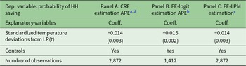
Table 2, panel A, presents a CRE estimate of households’ probability of saving on standardized temperature anomalies and other controls, including mean values of continuous explanatory variables. Accordingly, on average, an increase in temperature shock by 1 standard deviation causes the probability of saving to decrease by 1.4 per cent, and this result is statistically significant at the 1 per cent level. This reflects the short-run response of households’ saving to unexpected temperature shocks. In panels B and C, we estimate the effects of temperature anomalies on households’ probability of saving using FE logit and FE-LPM models, respectively. The results from these specifications are broadly consistent with the baseline estimates reported in panel A.
Impact of temperature shocks on households’ saving behaviour

Table 2 Long description
The table reports how deviations in temperature from the long-run average relate to the probability that a household saves, estimated with three approaches: correlated random effects, fixed-effects logit, and fixed-effects linear probability. In every panel, the temperature deviation coefficient is negative and very similar in size, around minus 0.014 to minus 0.015, indicating a small reduction in saving likelihood as temperature deviates from the long-run mean. Standard errors are small, about 0.002 to 0.003, suggesting the estimates are precise. All three models include control variables. Sample size differs by method: 2,872 observations in the correlated random effects and fixed-effects linear probability panels, and 1,412 in the fixed-effects logit panel. Because the models and samples differ, the coefficients are best compared as average partial effects rather than as raw model parameters.
a In panel A, control variables include standardized rainfall deviations from long-run(t) (LR (t)), experience of other shocks within a year, basic financial knowledge, distance to the nearest FFIs, receipt of remittance, ownership of off-farm income activity, marital status, religion of household (HH) head, age and age squared of HH head, dependency ratio, year dummy, regional dummies and the mean value of all continuous variables (i.e., standardized temperature and rainfall anomalies, age of HH head, distance to FFIs and dependency ratio).
b In panel B, all the above controls – except regional dummies, marital status, religion of the HH head and mean values of the continuous variables – are included.
c In panel C, all those controls mentioned under panel A – except regional dummies, religion of the HH head and mean values of the continuous variables – are included. Values in parentheses are standard errors and are clustered at 161 EAs. The full set of results, including all control variables, is reported in the online appendix Table A1.
d Mainly for two reasons, we base our discussion of results on average partial effects (APEs) derived from the CRE estimations rather than raw CRE coefficients. First, compared to raw CRE coefficients, which are structural parameters without a direct probability interpretation, APEs average individual-specific marginal effects or provide a population-level effect in terms of probability that are simpler to communicate (Abrevaya and Hsu, Reference Abrevaya and Hsu2021). In light of this, second, APEs coefficients enable, in some way, a better and more meaningful comparison between the within-unit effects found by FE-LPM estimations (which are marginal effects/probabilities on their own).
Consequently, all three panels in Table 2 are consistent in suggesting that, in rural Ethiopia, temperature shocks will be accompanied by reductions in the probability of households’ saving. Consistent with our finding, Churchill et al. (Reference Churchill, Trinh and Danquah2023) find that in Vietnam, households exposed to higher temperature shocks are also less likely to save.
We further extend our analysis to assess whether or not the impact of temperature shocks on saving behaviour, as presented in Table 2, panel A, depicts the long-term relationship between the two variables. To this end, we re-estimate our basic model by incorporating adaptation and intensification as specified in Equations (A10) and (A11), respectively (online appendix, Section B). Coefficient estimates from panel A of Table A2 (online appendix) do not signal clear evidence of adaptation to temperature shocks as far as their impact on households’ saving behaviour. Moreover, in panel B, all of the coefficient estimates that have been included to capture intensification are jointly statistically insignificant. Our findings may be explained by the fact that, as noted by Carleton and Hsiang (Reference Carleton and Hsiang2016), the impacts of high temperatures are immediate and severe, but quickly decay. However, inferences from our results for adaptation and intensification should be taken with caution, as we work only with two rounds of panel data, which limits the ability to capture long-term relationships.
5.2. Mediation analysis
In this section, we examine whether or not the main result, as presented in Table 2, panel A, is mediated by risk and time preferences. Our analysis also looks at the relative importance of these channels, compared to other economic mediators of the impact of temperature on households’ saving, such as labour productivity.Footnote 8 To this end, we follow the approach of Alesina and Zhuravskaya (Reference Alesina and Zhuravskaya2011) as applied by Churchill et al. (Reference Churchill, Smyth, Trinh and Yew2022) to estimate whether time and risk preferences mediate the relationship between saving decisions and temperature. Accordingly, to qualify as a mediator, risk preferences and time preferences must first exhibit a statistically significant response to temperature shocks. In addition, each candidate must be systematically correlated with households’ saving behaviour to satisfy the mediation criterion. Mediation is assessed by examining changes in the estimated effect of temperature shocks on savings following the inclusion of risk and time preferences as additional covariates. A reduction in the magnitude of the temperature shock coefficient indicates partial mediation, whereas full mediation is established if the coefficient becomes statistically insignificant once these preference measures are controlled for. In the online appendix Table A3, we present the estimates of time and risk preferences on temperature shocks and find statistically significant correlations.
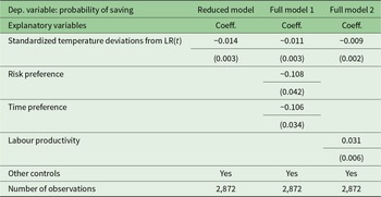
After we ascertain that there is a significant correlation between temperature shocks and both time and risk preferences among Ethiopian rural households, we estimate an FE-LPMFootnote 9 version of Equation (9) by incorporating time and risk preferences to determine whether or not these variables are responsible for channelling the impact of temperature shocks on households’ saving behaviour. As illustrated in Table 3 (i.e., full model 1), both risk-taking and impatience correlate with household’s likelihood of saving. More specifically, the probability that risk-taking households will save falls by 10.8 per cent compared to non-risk-taking households. For impatient households, the saving probability is 10.6 per cent lower than that of non-impatient households. Individuals with high discount rates are less committed to saving for the future. This supports the findings of Falk et al. (Reference Falk, Becker, Dohmen, Enke, Huffman and Sunde2018), who questioned 80,000 respondents in 76 countries and found that a higher level of patience was linked to a higher likelihood of saving.
Mediation results: FE-LPM estimation

Table 3 Long description
The table reports fixed effects linear probability estimates for the dependent variable, probability of saving, comparing a reduced model with two fuller specifications. Standardized temperature deviations are negative and statistically precise in all three models, with coefficients of minus 0.014 in the reduced model, minus 0.011 when preferences are added, and minus 0.009 when labor productivity is added. In the first full model, risk preference and time preference are both negatively associated with saving, at minus 0.108 and minus 0.106, respectively. In the second full model, labor productivity is positively associated with saving, with a coefficient of 0.031. Other controls are included in every model, and each model uses 2,872 observations. Standard errors are reported in parentheses and are clustered, so uncertainty reflects within cluster correlation; coefficients should be interpreted as associations rather than causal effects.
LR, long-run.
Notes: Controls include all those mentioned for panel A of Table 2. Values in parentheses are standard errors, which are also clustered at 161 EAs.
We can also infer from Table 3 that both risk and time preference combined channel approximately 21 per centFootnote 10 of the impact of temperature shocks on savings. Full model 2 in Table 3 shows how labour productivity correlates with households’ saving behaviour. As mentioned in Section 1, we include this in our regression in order to illustrate the importance of behavioural channels relative to a well-established economic channel (i.e., labour productivity). The result signals that labour productivity correlates positively with households’ saving behaviour. It channels nearly 35 per cent of the impact of temperature anomalies on households’ savings, which exceeds the amount channelled by risk and time preferences combined. However, we should not discount the significance of behavioural factors, as these variables play a role as partial mediators.
5.3. Heterogeneity effects
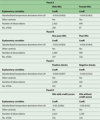
In this section, we assess whether or not the impact of temperature shocks, as presented in Table 2, shows heterogeneity in savings for some socio-economic characteristics and different types of temperature anomalies. Accordingly, first we examine whether the results vary between male- and female-headed households. As shown in Table 4, panel A, the results for male and female heads do not vary, as both groups’ savings respond similarly for temperature anomalies.
Heterogeneous impacts of temperature shocks: dependent variable is household’s probability of saving-CRE estimation with APE coefficients

Table 4 Long description
The table reports average partial effect coefficients from a CRE model for how standardized temperature deviations from a long-run level relate to a household’s probability of saving, split into four subgroup panels. In Panel A, the temperature effect is negative and the same size for male-headed and female-headed households, both about minus 0.014 with a standard error of 0.003. In Panel B, the effect is more negative for poor households, about minus 0.016 with a standard error of 0.004, than for non-poor households, about minus 0.012 with a standard error of 0.003. In Panel C, both positive and negative temperature shocks are associated with larger declines in saving probability, about minus 0.029 with a standard error of 0.007 for positive shocks and about minus 0.033 with a standard error of 0.021 for negative shocks. In Panel D, households without credit access show a much larger negative association, about minus 0.03 with a standard error of 0.01, compared with households with credit access, about minus 0.01 with a standard error of 0.002. All panels include other controls, and sample sizes and clustered enumeration areas vary by subgroup, including a notably small cluster count for negative shocks.
LR, long-run; HH, household.
Note: Controls include all those mentioned for panel A of Table 2.
Second, we expand our analysis to include a more crucial factor: the effect of temperature shocks on the saving habits of poor and non-poor households. We find that temperature shocks reduce the likelihood of saving to a greater extent among poor households than among non-poor households (panel B). More specifically, a change in temperature anomalies by 1 standard deviation reduces the poor households’ likelihood of saving by 1.6 per cent, whereas the same shock reduces non-poor households’ probability of saving by 1.2 per cent. We notice that poor households are more impatient compared to their counterparts, which may partly explain the disparity in the results.
Third, we explore heterogeneity in the effects of climate shocks by distinguishing between the types of temperature anomalies following Dell et al. (Reference Dell, Jones and Olken2014), who indicate that impacts of temperature shocks on households’ saving behaviour may differ depending on whether households experience positive or negative deviations from historical norms. To examine this possibility, we estimate separate regressions for households exposed to positive and negative temperature shocks. The results, reported in Table 4, panel C, indicate that both types of shocks are associated with a lower likelihood of saving. However, only the effect of positive temperature shocks is statistically significant. This finding also suggests that the aggregate effect reported in Table 2, panel A, is primarily driven by positive temperature anomalies (i.e., actual records surpass long-run mean temperature records).
Finally, we expand our heterogeneity analysis of temperature anomalies’ impact on those households with and without credit access. This aspect helps to delve into the analysis of savings’ response in the presence of another shock-coping mechanism – access to credit. As shown in Table 4, panel D, the magnitude of reduction in probability of saving for those households without credit access is nearly twofold higher compared to those with credit access.
5.4. Robustness checks
In this section, we evaluate the robustness of our main result in Table 2, panel A, to alternative measures of temperature shock and data source, outcome variable and estimation approaches. First, in the online appendix Table A4, we present various measurements of temperature shocks in addition to standardized deviations and Climate Engine data source. Accordingly, panel A demonstrates the impact of temperature shocks, measured by degree-days (hot and cold), on households’ saving behaviour. Degree-days have the advantage of capturing both intensity and duration of temperature shocks compared to deviations (Schlenker and Roberts, Reference Schlenker and Roberts2009). To this end, we extract daily temperature from the European Centre for Medium-Range Weather Forecasts ERA5 since Climate Engine/Terra Climate has no such data set. The ERA5 dataset is produced on a global grid with a spatial resolution of 0.25° × 0.25°, which is approximately equal to 31 km × 31 km at the equator (Michler et al., Reference Michler, Josephson, Kilic and Murray2022). Owing to its high temporal resolution and physical consistency, ERA is widely used for climate analyses that anchor on daily information (Hersbach et al., Reference Hersbach, Bell, Berrisford, Hirahara, Horányi, Muñoz-Sabater, Nicolas, Peubey, Radu, Schepers and Simmons2020). We extract daily temperature for the years 2014 and 2018 (i.e., the survey years) and from this, we calculate hot and cold degree-days.Footnote 11 Seppanen et al. (Reference Seppanen, Fisk and Lei2006) have assessed previous studies and observed that actual temperature records above 25°C are significantly and negatively correlated with various indicators of workers’ performance. Hence, we rely on this to define hot and cold degree-days. Estimated coefficients in Table A4, panel A, show that hot degree-days reduce the households’ probability of saving significantly. Even though we observe that cold degree-days reduce households’ probability of saving, the coefficient estimate is not statistically significant.
In panel B, we extend our robustness analysis of the response of households’ saving to temperature anomalies, measured by level deviations (i.e., actual temperature at time  $t$ minus the long-run mean temperature). Despite the fact that this measure of temperature shock limits comparability across different EAs, which exhibit high heterogeneity due to varied topography and agroecology, it offers a key advantage of interpretability for policymakers, as the coefficient estimates correspond directly to observable changes in degrees Celsius (Auffhammer et al., Reference Auffhammer, Hsiang, Schlenker and Sobel2013). Using this measure, we find that, on average, an increase in temperature anomalies by 1°C reduces the likelihood of rural households’ saving by approximately 1.2 per cent, showing that our main result is robust to this alternative measure of temperature shock.
We further extend our robustness analysis by conducting the falsification (placebo) test. Specifically, we regress current household’s saving on future realization of weather shocks, in which the result should be insignificant because households’ saving behaviour should not respond to future weather shocks that have not yet occurred. As expected, the estimates in panel C show that this coefficient estimate is statistically insignificant.
When climate variables constitute the primary explanatory variables of interest, Michler et al. (Reference Michler, Josephson, Kilic and Murray2022) and Josephson et al. (Reference Josephson, Michler, Kilic and Murray2025) suggest that it is important to assess the robustness of empirical findings to alternative climate data sources. Guided by this insight, we re-estimate our main specification using an alternative temperature dataset derived from the MERRA-2 (Modern-Era Retrospective Analysis for Research and Applications, Version 2) produced by NASA. The MERRA-2 dataset provides monthly temperature data at a spatial resolution of 0.5° latitude by 0.625° longitude, corresponding to approximately 55 km × 69 km at the equator (Michler et al., Reference Michler, Josephson, Kilic and Murray2022). Using this dataset, we reconstruct our temperature variable following the same procedure outlined in Section 3 to ensure comparability with our baseline specification, which relies on Climate Engine/Terra Climate data at a much finer spatial resolution (approximately 4 km × 4 km at the equator).
The result, reported in panel E of Table A4 (online appendix), indicates that our main coefficient of interest remains qualitatively consistent when using MERRA-2 data. Although the estimated magnitude is somewhat attenuated and statistical significance decreases to the 5 per cent level, the overall pattern of results aligns closely with our baseline findings. The observed attenuation in coefficient magnitude and precision is likely attributable to differences in spatial resolution. In particular, the relatively coarser spatial resolution of MERRA-2 implies that each grid cell aggregates weather conditions over a broader geographic area, which may smooth out localized temperature variations (Auffhammer et al., Reference Auffhammer, Hsiang, Schlenker and Sobel2013). This aggregation can, in turn, attenuate the estimated magnitude of the coefficients.
Second, we assess the robustness of our results using alternative measures of our outcome variable – the self-reported status of saving practice by households. In the first place, we generate a dummy variable with a value equal to 1 if a household’s income is greater than consumption expenditure (i.e., positive saving) and 0 otherwise, following prior approaches in the literature by Heckman and Hanna (Reference Heckman and Hanna2015), which is less susceptible to subjective reporting biases and hence provides an objective proxy for households’ saving behaviour. As per this indicator, nearly 29 per cent of households practise savings, which is a lower rate as compared to self-reported status of households’ saving behaviour. Using this alternative measure, the estimated result in Table A5, panel A (online appendix) shows that using temperature anomalies measured by standardized deviation reduces the likelihood of households’ saving, a result consistent with our main finding.
Next, we take the amount of savings as our dependent variable instead of a dummy variable for the saving behaviour indicator. This approach has the advantage of capturing the intensity of savings. To this end, we anchor on both the self-reported savings amount and residual savings (income left from food consumption expenditure). To address the skewness commonly observed in savings distributions, we use the logarithmic transformations of these measures. As illustrated in Table A5, panels B and C, an additional increase in temperature anomalies by 1 standard deviation reduces the amount of residual and self-reported household’s savings by 0.2 and 0.8 per cent, respectively.
Third, we assess the robustness of our main results to alternative estimation strategies, specifically by addressing potential sample attrition and accounting for spatial correlation in the error terms following Conley (Reference Conley1999). Attrition between survey rounds may introduce bias if it is systematic rather than random, thereby affecting the consistency of coefficient estimates (Wooldridge, Reference Wooldridge2010). In our case, attrition, which mainly arises in the second survey round (2018), necessitates dropping the corresponding households from the baseline sample (2014) to maintain a balanced panel. To examine whether attrition is non-random, we follow the approach used by Makate et al. (Reference Makate, Angelsen, Holden and Westengen2024). Specifically, we estimate a probit model of attrition, where the dependent variable equals 1 if a household observed in the baseline survey is not reinterviewed in the follow-up round, and 0 otherwise (we have 64 attriting vs 1.436 non-attriting households). As highlighted in Behr (Reference Behr2006), we conceptualize attrition by conditioning wave  $t$ outcomes on response behaviour in wave $t + 1$. The model uses baseline household characteristics as predictors, and the variables included in the probit model comprise socio-demographic characteristics – such as the sex, age (and its square), family size, religion and years of schooling of the household head – as well as economic indicators, including landholding size, livestock ownership (measured in tropical livestock units), household labour endowment, engagement in off-farm income-generating activities and receipt of remittances. Given that income data are missing for a significant number of attriting households, we rely on these observable proxies for productive capacity and income-generating potential. The estimation results (see online appendix Table A6) indicate that age, years of schooling and participation in off-farm activities are significant predictors of attrition, suggesting that attrition is not entirely random.
In the second step, we use the estimated probit model to predict each household’s probability of remaining in the sample and construct inverse probability weights (IPWs) as the inverse of these predicted probabilities. In this context, observations with a lower predicted probability of remaining in the sample are assigned higher weights. As noted by Behr (Reference Behr2006) and Wooldridge (Reference Wooldridge2010), this reweighting procedure helps restore the representativeness of the sample by giving greater influence to observations that resemble those more likely to attrit.
Finally, we incorporate the constructed IPW (which is a time-invariant variable since IPW for a household is the same in both waves) into our main regression model to test and control for potential attrition bias. We report results using stabilized inverse probability weights (SIPWs), as recommended in Cole and Hernan (Reference Cole and Hernan2008), alongside estimates based on the inverse Mills ratio (IMR), derived using a similar selection-correction framework. As shown in Table A7 (online appendix), neither the SIPW nor IMR terms are statistically significant, suggesting that attrition does not pose a major threat to the validity of our estimates. As far as testing for differential attrition with respect to baseline temperature exposure (our main variable of interest) is concerned, we conduct t-test for equality of mean standardized temperature deviation between attriting and non-attriting households. The result suggests that we have to accept the equality of the two means (t-value = 0.2563), which implies no meaningful differences between attriting and non-attriting households based on baseline temperature shocks.
Next, beyond clustering standard errors at the EA level, we further strengthen our inference by implementing spatially robust standard errors following Conley (Reference Conley1999). This approach explicitly accounts for spatial (and, where relevant, temporal) dependence in the error structure, which is particularly important in our setting. Climate variables such as temperature shocks tend to exhibit strong spatial correlation, implying that observations located in close geographic proximity are likely to experience similar shocks and, consequently, correlated standard errors (Dell et al., Reference Dell, Jones and Olken2014). While clustering at the EA level partially addresses within-cluster correlation, it may be insufficient when correlation extends beyond administrative boundaries, as is typical with climate shocks. Failure to account for such spatial dependence can lead to downward-biased standard errors and over-rejection of null hypotheses, thereby overstating statistical significance (Conley, Reference Conley1999).
To address this concern, we re-estimate our main specification using Conley (Reference Conley1999) standard errors with alternative spatial cut-off distances. Specifically, Table A8 (online appendix) reports coefficient estimates using a baseline cut-off of 100 km (panel A), as commonly adopted in the literature, and a more conservative cut-off of 200 km (panel B), allowing for broader spatial dependence. Across both specifications, we observe a slight increase in standard errors relative to the EA-clustered estimates. However, these adjustments are not sufficiently large to alter the statistical significance of our main coefficient of interest, which remains significant at the 1 per cent level; this provides additional confidence that our main results are not driven by unaddressed spatial correlation in the error terms.
6. Summary and conclusions
Ethiopia has been facing climate shocks and extremes, including frequent droughts. When attempting to confront the challenges of climate change, policymakers must take into consideration its multifaceted impacts. In this study, we assess the impacts of climate shocks on households’ saving behaviour in rural Ethiopia. Savings are key to consumption smoothing, central to financing productive investments in modern agricultural inputs, facilitating income diversification of rural households. Moreover, savings are fundamental to households’ long-term welfare by enabling sustained investment in both physical and human capital.
We conduct our assessment by combining satellite temperature data from Climate Engine/Terra Climate with two rounds of panel survey data. Our results demonstrate that current temperature anomalies from the long-run mean measured by standardized deviations cause the probability of rural households’ saving to decline. Our result is robust with respect to alternative measures of saving behaviour, temperature shocks and estimation techniques. Hence, it is crucial to account for the impact on financial outcomes, such as savings, when measuring the damage costs caused by climate shocks to the economy.
Mediation analysis of time and risk preferences shows that both variables channel the impact of temperature shocks on households’ saving. We also observe that temperature shocks correlate positively with risk-taking and impatience, and in turn these behaviours negatively correlate with households’ saving. This suggests that households exhibiting high time discounting or high propensity for risk are less inclined to allocate resources towards the future. Consequently, preserving long-term welfare requires the promotion of commitment-based saving instruments, including saving mechanisms with automatic deductions at harvest time.
Finally, compared to their counterparts, poor households’ saving behaviour and those without credit access are more affected by temperature shocks. Therefore, policy measures that try to lessen or mitigate the detrimental consequences of climate change on household financial status should concentrate more on these groups.
Supplementary material
The supplementary material for this article can be found at https://doi.org/10.1017/S1355770X26100618.
Acknowledgements
The authors are grateful to the Association of Ethiopian Microfinance Institutions (AEMFI) and the then Federal Democratic Republic of Ethiopia (FDRE) Policy Studies and Research Institute (PSRC), now the Policy Studies Institute (PSI), for granting access to and allowing use of their datasets for this research. We also thank the associate editor and two anonymous reviewers for their suggestions and comments, which have led to improvement of the current version of the manuscript. Moreover, we used ChatGPT to rewrite a few of our sentences to improve readability.
Competing interests
The authors declare none.






 Open access

