





1. Introduction
The placement of viscoplastic fluids within a target region of a medium has numerous applications across various industries, such as coating (Smit et al. Reference Smit, Kusina, Colin and Joanny2021), packaging (Rasschaert et al. Reference Rasschaert, Talansier, Blésès, Magnin and Lambert2018), additive manufacturing (Geffrault et al. Reference Geffrault, Bessaies-Bey, Roussel and Coussot2023; Arab et al. Reference Arab, Louna, Mahfoud, de Souza Mendes, Garcia-Blanco and Franco2024, Reference Arab, Louna, Mahfoud, de Souza Mendes, Garcia-Blanco and Franco2025) and oil and gas well cementing (Faramarzi et al. Reference Faramarzi, Akbari and Taghavi2024; Akbari et al. Reference Akbari, Frigaard and Taghavi2024). These fluids exhibit yield-stress and shear-thinning behaviours (Frigaard Reference Frigaard2019). Depending on the application, they may be placed in flow geometries filled completely or partially with another fluid, usually with density and viscosity contrasts between the fluids involved. The variation in physical and rheological properties leads to buoyancy forces and variations in viscous and inertial stresses, which can result in complex placement flow dynamics. The topic of the current work is the flow of a miscible dense viscoplastic fluid after placement on top of a less dense Newtonian fluid in vertical and inclined (closed) pipes. Our aim is to study post-placement dynamics in terms of general flow behaviours, interface evolution, concentration and velocity profiles, mixing behaviour, interface front velocities and dynamics.
The placement of a dense fluid on top of another (less dense) fluid is a density-unstable situation, in which an exchange flow between the fluids happens (Debacq et al. Reference Debacq, Fanguet, Hulin, Salin and Perrin2001; Picchi et al. Reference Picchi, Suckale and Battiato2020; Ungarish Reference Ungarish2024). Buoyant exchange flows experience mixing in most inclination angles, leading to an inefficient exchange/removal regime (Debacq et al. Reference Debacq, Hulin, Salin, Perrin and Hinch2003). Birman et al. (Reference Birman, Battandier, Meiburg and Linden2007) have numerically studied the effects of the inclination on the density-unstable exchange flow in a two-dimensional (2-D) channel verified by experimental observations of lock-exchange flows in a tube of circular cross-section. The simulations showed that the inertially controlled flow goes through an initial quasi-steady phase that is characterised by a constant front velocity, which has a maximum for inclination angle of $\approx 40^{\circ }$
. After persisting over a finite initial development distance, the flow subsequently undergoes a transition to a second phase with a larger, unsteady, front velocity. They have also observed a situation where the fluid layers behind the front move faster than the front itself. Initially, the resulting addition of fluid to the front from behind affects only the size of the front, while its velocity remains unchanged. Eventually, the fluid front is unable to absorb more fluid from behind and its velocity has to increase, thereby triggering the transition to the second, unsteady, phase. The transition time is determined as a function of the inclination angle and density ratio of the two fluids. Buoyant exchange flows of viscous fluids within a horizontal channel were studied theoretically and experimentally by Matson & Hogg (Reference Matson and Hogg2012), exploring how the viscosity ratio of the two fluids affects the evolution of the shape of the interface between them. In addition to the above-mentioned studies, there exist also a range of useful studies on the effects of buoyancy and viscosity ratio on the exchange flow dynamics (Séon et al. Reference Séon, Hulin, Salin, Perrin and Hinch2004, Reference Séon, Znaien, Perrin, Hinch, Salin and Hulin2007; Kerswell Reference Kerswell2011; Beckett et al. Reference Beckett, Mader, Phillips, Rust and Witham2011; He et al. Reference He, Zhu, Zhao, Chen, Lin and Yuan2021).
$\approx 40^{\circ }$
. After persisting over a finite initial development distance, the flow subsequently undergoes a transition to a second phase with a larger, unsteady, front velocity. They have also observed a situation where the fluid layers behind the front move faster than the front itself. Initially, the resulting addition of fluid to the front from behind affects only the size of the front, while its velocity remains unchanged. Eventually, the fluid front is unable to absorb more fluid from behind and its velocity has to increase, thereby triggering the transition to the second, unsteady, phase. The transition time is determined as a function of the inclination angle and density ratio of the two fluids. Buoyant exchange flows of viscous fluids within a horizontal channel were studied theoretically and experimentally by Matson & Hogg (Reference Matson and Hogg2012), exploring how the viscosity ratio of the two fluids affects the evolution of the shape of the interface between them. In addition to the above-mentioned studies, there exist also a range of useful studies on the effects of buoyancy and viscosity ratio on the exchange flow dynamics (Séon et al. Reference Séon, Hulin, Salin, Perrin and Hinch2004, Reference Séon, Znaien, Perrin, Hinch, Salin and Hulin2007; Kerswell Reference Kerswell2011; Beckett et al. Reference Beckett, Mader, Phillips, Rust and Witham2011; He et al. Reference He, Zhu, Zhao, Chen, Lin and Yuan2021).
The presence of a yield-stress fluid in a buoyant exchange or displacement flow can affect the flow patterns observed. For instance, Varges et al. (Reference Varges, Fonseca, Costa, Naccache, de Souza Mendes and Pinho2018) have observed three different flow regimes, namely unstable, quasi-stable and stable (no flow) in experimental analysis of the immiscible exchange flow between a more dense elasto-viscoplastic fluid above a less dense Newtonian oil in a vertical pipe. They have found that for the quasi-stable regime, a slow plug flow starts after a time delay, which is a result of thixotropic and elastic effects of the more dense fluid. For the unstable regime, a wavy core–annular flow with the denser fluid in the core region was observed. Akbari & Taghavi (Reference Akbari and Taghavi2022a , Reference Akbari and Taghavib ) have observed breakup, coiling and bulging flow regimes when a viscoplastic fluid is injected into a closed-end pipe filled with a Newtonian fluid. Malekmohammadi et al. (Reference Malekmohammadi, Naccache, Frigaard and Martinez2010) have studied the buoyancy-driven exchange flow of two non-Newtonian fluids in a horizontal closed pipe using experiments and numerical simulations. The more dense fluid has only shear-thinning behaviour while the less dense fluid has also yield stress. They have investigated the effects of buoyancy, inclination close to horizontal and yield stress on the interface shape and length of slumping the more dense fluid. It was found that decreasing the yield stress of the less dense fluid leads to extending the slump length.
The specific industrial applications of our study originate from the cementing processes in the decommissioning of oil and gas wells: so-called plug and abandonment (P&A). The P&A operation is run to avoid oil and gas leakages to the surrounding environment, water aquifers and atmosphere (Trudel et al. Reference Trudel, Bizhani, Zare and Frigaard2019; Khalifeh & Saasen Reference Khalifeh and Saasen2020; Cahill & Samano Reference Cahill and Samano2022). Many oil and gas wells are not properly plugged for several reasons, such as cement slurry contamination, unfavourable mixing and poor in situ fluid displacement (Miranda et al. Reference Miranda2007). This can lead to potential pathways for leakage that require costly re-plugging operations. Therefore, it is necessary to improve P&A cementing operations. In many operations, the cement slurry is placed on top of a mechanical support, but in others the cement is pumped straight into the well, displacing the fluid that is present, called off-bottom placement (Nelson & Guillot Reference Nelson and Guillot2006; Khalifeh & Saasen Reference Khalifeh and Saasen2020). Off-bottom placement is more interesting from a fluid mechanics perspective, as the more dense yield-stress fluid (cement slurry) is placed on top of a less dense Newtonian fluid (typically water), which is evidently mechanically unstable. Vertical and inclined wells are treated.
In the context of fluid mechanics studies of the off-bottom method, Charabin & Frigaard (Reference Charabin and Frigaard2024) have experimentally studied the buoyancy-driven exchange flows in a vertical pipe, where the upper and lower fluids are a more dense viscoplastic fluid and a less dense Newtonian fluid, respectively. They have observed no sustained fluid flows for an adequately large yield number ( $Y$
), which denotes the ratio of yield stress to buoyancy stress. For smaller values of
$Y$
), which denotes the ratio of yield stress to buoyancy stress. For smaller values of $Y$
, a transition to an exchange flow regime occurs, where the less dense Newtonian fluid penetrates upwards into the viscoplastic fluid as a central finger with appearance of three regimes, namely helical finger, disconnected finger and slug flow. The transition between regimes was analysed based on inertial, viscous and buoyancy stresses.
$Y$
, a transition to an exchange flow regime occurs, where the less dense Newtonian fluid penetrates upwards into the viscoplastic fluid as a central finger with appearance of three regimes, namely helical finger, disconnected finger and slug flow. The transition between regimes was analysed based on inertial, viscous and buoyancy stresses.
Ghazal & Karimfazli (Reference Ghazal and Karimfazli2021, Reference Ghazal and Karimfazli2022) have utilised numerical simulations to develop a mechanistic understanding of fluid injection and displacement via a 2-D model. They examined the injection of a viscoplastic fluid through a centralised injector into a channel filled with a less dense Newtonian fluid. Their findings show that the injected fluid initially displaces the Newtonian fluid, forming a finger-like interface beneath the injector. The parallel shear flow that develops in this region is unstable, leading to interfacial instabilities that disrupt the downstream flow. As a result, a mixed layer forms below the injector as the viscoplastic finger breaks up.
As explained above, despite a large number of existing studies in the literature on buoyant exchange and displacement flows, the analysis of buoyant miscible exchange flows at high viscosity ratios is still lacking, which sets the motivation of our contribution. Our study, examines experimentally and numerically the flow dynamics of buoyant exchange flow of a more dense viscoplastic fluid after placement on top of a less dense Newtonian fluid in an inclined pipe. Flow visualisation experiments and complementary numerical simulations are performed in order to identify the flow features, such as the concentration of both fluids, which provides a complete spatiotemporal concentration map of the flow domain, velocity field the penetration front velocities, and the flow regimes for some parameter ranges. Detailed analysis of observed flow regimes, effects of tilted pipe on the exchange flow dynamics as well as further analysis of the viscoplastic fluid once it flows down the pipe are the new areas of this study in comparison with previous work (Charabin & Frigaard Reference Charabin and Frigaard2024). In addition to providing a fundamental understanding, the results of this study can ultimately contribute to improving the off-bottom P&A method, e.g. by enhancing the cement plug placement, improving the cement plug stability, ensuring quality performance during cementing operations and promoting safer operations.
The rest of this paper is structured as follows. In § 2, we present the description of the experimental set-up, non-intrusive measurement technique, fluid preparations and rheological characterisations, and complementary numerical simulations. In § 2.3, we describe the scope of our study, in terms of the governing dimensionless numbers. In § 3, we first demonstrate some general flow behaviours, and then focus on the details of the observed flow regimes and highlight the effects of the buoyancy number ( $\chi$
), yield number (
$\chi$
), yield number ( $Y$
) and inclination angle (
$Y$
) and inclination angle ( $\beta$
) on the flow dynamics. We also elaborate on the front velocity of both Newtonian and viscoplastic fluids. Finally, in § 4, we conclude the study with a brief summary.
$\beta$
) on the flow dynamics. We also elaborate on the front velocity of both Newtonian and viscoplastic fluids. Finally, in § 4, we conclude the study with a brief summary.
Schematic view of the experimental set-up. The shape of the fluid interface is illustrative only.

2. Methodology and scope of the study
2.1. Experimental set-up
Our experimental apparatus consists of a long transparent closed-end pipe with a diameter of 1.95 (cm) and a length of 315 (cm), as depicted in figure 1. The set-up is fixed on a structure that can be tilted at different inclination angles from vertical to horizontal. The two fluids are initially separated by a gate valve (with a blade thickness of 1 mm) positioned in the middle of the pipe and oriented perpendicular to the pipe axis. To minimise mechanically induced mixing and precisely define the onset of the experiment, the valve is pneumatically operated using air pressure, which allows the gate to be retracted completely in approximately 0.1 s, a time scale significantly shorter than the characteristic time scale of the buoyancy-driven flow, thereby ensuring the initial perturbation is primarily driven by the physical fluid mechanics rather than mechanical drag. Two pumps are connected to the pipe to transfer the fluids into it. Light-emitting diodes are positioned behind the pipe to create a uniform lighting across the pipe, with diffusive panels placed in between. Light absorption calibrations are performed, for which before each experiment, an image of the pipe filled with the transparent, more dense fluid and an image of the pipe containing the darker, less dense fluid are recorded. These are used as references of light intensities for the Beer–Lambert law, in order to eventually find normalised concentration fields (Akbari & Taghavi Reference Akbari and Taghavi2021, Reference Akbari and Taghavi2023).
Dimensional parameters and ranges used in our experiments; the $\boldsymbol{\hat{\cdot}}$
accent denotes a dimensional variable.
$\boldsymbol{\hat{\cdot}}$
accent denotes a dimensional variable.

Table 1. Long description
The table has three columns: Parameter, Name, and Range (unit). It contains 11 rows, each representing a different parameter used in the experiments. The parameters include the inner radius of the pipe, pipe length, fluid densities, fluid viscosity, yield stress, fluid consistency, gravitational acceleration, molecular diffusivity, and power-law index. Each row lists the parameter name, its corresponding range, and the unit of measurement. The table provides specific values and ranges for each parameter, which are essential for understanding the experimental setup.
The experimental procedure involves filling the lower half of the pipe with Newtonian fluid (pure water as a less viscous, less dense fluid), and feeding the upper half via a viscoplastic fluid (as a more viscous, more dense fluid). For visualisation purposes, the Newtonian fluid is dyed with 525 (mg l−1) of ink (Fountain Pen India black ink). Before starting the experiment, the inclination angle is adjusted. Upon opening the gate valve, depending on the fluid properties and the pipe inclination angle, either an exchange flow occurs or no flow. Two cameras (Nikon Z5), each capturing half of the pipe, record the flow at a resolution of 5472 $\times$
3084 pixels and a moderate frame rate (
$\times$
3084 pixels and a moderate frame rate ( $\approx 25$
frames per second). This provides direct visualisation of the fluid–fluid interface and mixing between the fluids. A computer acquisition system is used throughout the experiments for recording the flow images. The collected images are processed using an in-house MATLAB image processing code, to analyse the flow details.
$\approx 25$
frames per second). This provides direct visualisation of the fluid–fluid interface and mixing between the fluids. A computer acquisition system is used throughout the experiments for recording the flow images. The collected images are processed using an in-house MATLAB image processing code, to analyse the flow details.
The camera images are interpreted using a light-attenuation technique driven by uniform back-lighting panels. The cameras capture the light transmitted directly through the fluid column. To ensure an accurate measurement, the ink concentration in the dyed fluid is calibrated to be translucent; it is optically dense enough to provide high contrast, but thin enough to avoid total light blockage across the full pipe diameter, thereby maintaining a predictable correlation between light intensity and fluid concentration. Furthermore, because the pipe has a circular cross-section, the path length of the transmitted light varies across the transverse axis. To correct for this varying optical depth, the raw experimental images are normalised pixel-by-pixel against two reference calibration images: one acquired with the test section completely filled with the transparent fluid ( $C=0$
) and the other with the test section completely filled with the dyed fluid (
$C=0$
) and the other with the test section completely filled with the dyed fluid ( $C=1$
). This normalisation process inherently accounts for the circular geometry, allowing the 2-D pixel intensities to be accurately converted into the depth-integrated concentration field.
$C=1$
). This normalisation process inherently accounts for the circular geometry, allowing the 2-D pixel intensities to be accurately converted into the depth-integrated concentration field.
In total, around 70 placement flow experiments are performed, for a range of different experimental parameters: different inclinations, fluid rheological properties and density differences. The dimensions of the experimental set-up and the range of flow parameters are given in table 1.
2.2. Fluid preparations and rheological characterisations
A transparent viscoplastic fluid is prepared by dissolving a small amount of Carbopol in water. To adjust the rheology of the more dense fluid, different Carbopol solution concentrations, with weight percent (wt%) of 0.015–0.1, are used. A systematic preparation protocol is followed. First, sugar is added to 20 litres of water to increase the density of the solution and give a desired density difference between the fluid pairs. The fluid density is measured using a high-precision density meter (Anton Paar DMA 35) at an ambient temperature of about 24–25 ( $^\circ$
C). Then, Carbopol 940 powder is dissolved into the dense solution while being mixed at 300 (rpm) for 2 hours using a EUROSTAR 60 mixer equipped with a three-bladed stainless steel blade to prevent clumping during the mixing process (Eslami et al. Reference Eslami, Akbari and Taghavi2022). After the Carbopol powder is completely dissolved, the low-viscosity acidic solution is kept at rest for 12 hours. Because the fluid has not yet developed a yield stress at this stage, this resting period allows any trapped air bubbles to freely escape. Then, the solution is neutralised to reach pH
$^\circ$
C). Then, Carbopol 940 powder is dissolved into the dense solution while being mixed at 300 (rpm) for 2 hours using a EUROSTAR 60 mixer equipped with a three-bladed stainless steel blade to prevent clumping during the mixing process (Eslami et al. Reference Eslami, Akbari and Taghavi2022). After the Carbopol powder is completely dissolved, the low-viscosity acidic solution is kept at rest for 12 hours. Because the fluid has not yet developed a yield stress at this stage, this resting period allows any trapped air bubbles to freely escape. Then, the solution is neutralised to reach pH $\approx$
7 by adding an appropriate amount of sodium hydroxide as a base agent, i.e. 0.29 g of NaOH (Fisher BioReagents) per 1 g of Carbopol powder. During this neutralisation stage, the solution is stirred carefully for one hour to avoid any new air entrainment. The Carbopol polymer chains can be negatively charged due to the addition of NaOH; consequently, the charged chains repel one another and, as the polymer structures swell and jam, the solution finally changes into a gelled material (i.e. with yield stress) (Jørgensen et al. Reference Jørgensen, Le Merrer, Delanoë-Ayari and Barentin2015).
$\approx$
7 by adding an appropriate amount of sodium hydroxide as a base agent, i.e. 0.29 g of NaOH (Fisher BioReagents) per 1 g of Carbopol powder. During this neutralisation stage, the solution is stirred carefully for one hour to avoid any new air entrainment. The Carbopol polymer chains can be negatively charged due to the addition of NaOH; consequently, the charged chains repel one another and, as the polymer structures swell and jam, the solution finally changes into a gelled material (i.e. with yield stress) (Jørgensen et al. Reference Jørgensen, Le Merrer, Delanoë-Ayari and Barentin2015).
Rheological measurements of the Carbopol solutions are performed using a Malvern Kinexus rheometer. A parallel-plate geometry with a 40 (mm) plate diameter at a gap of 1 (mm) is employed for flow curve measurements. The rheology is measured at the same temperature as reported during actual flow experiments, in the range of $\approx$
25 (
$\approx$
25 ( $^\circ$
C) with
$^\circ$
C) with $\pm$
0.1 (
$\pm$
0.1 ( $^\circ$
C) uncertainty. To reduce the influence of wall slip during the rheometry measurements at low shear rates, rough sandpapers are attached to the rheometer plates (Mitishita et al. Reference Mitishita, Alishahi and Frigaard2023). Before each test, the sample of Carbopol gel is pre-sheared at 100 (s
$^\circ$
C) uncertainty. To reduce the influence of wall slip during the rheometry measurements at low shear rates, rough sandpapers are attached to the rheometer plates (Mitishita et al. Reference Mitishita, Alishahi and Frigaard2023). Before each test, the sample of Carbopol gel is pre-sheared at 100 (s $^{-1}$
) for 30 (s), followed by a rest period of 30 (s) at 0 (Pa). Pre-shear followed by a rest before each rheometry test erases the sample’s previous shear history (Wang et al. Reference Wang, Sutyak, Oladeji, Rogers and Krogstad2025), ensuring reproducible initial conditions while creating a homogeneous, uniform gel and reducing concentration gradients. This procedure also allows trapped air bubbles, formed during Carbopol gel preparation or sample loading on the rheometer plates, to escape. The subsequent rest allows the material structure to rebuild, so measurements reflect the true equilibrium viscoplastic behaviour.
$^{-1}$
) for 30 (s), followed by a rest period of 30 (s) at 0 (Pa). Pre-shear followed by a rest before each rheometry test erases the sample’s previous shear history (Wang et al. Reference Wang, Sutyak, Oladeji, Rogers and Krogstad2025), ensuring reproducible initial conditions while creating a homogeneous, uniform gel and reducing concentration gradients. This procedure also allows trapped air bubbles, formed during Carbopol gel preparation or sample loading on the rheometer plates, to escape. The subsequent rest allows the material structure to rebuild, so measurements reflect the true equilibrium viscoplastic behaviour.
The rheological parameters and density of the Carbopol solutions, obtained by fitting the stress–shear-rate curves to the HB model (equation (2.1)).

Table 2. Long description
A table with ten rows and five columns. The columns are labeled Sample, τy (Pa), k̂ (Pa sn), n, and ρ̂H (kg m-3). The table presents the rheological parameters and density of Carbopol solutions. Row 1: Sample I, τy 9.80, k̂ 9.71, n 0.46, ρ̂H 1050. Row 2: Sample II, τy 3.25, k̂ 1.83, n 0.56, ρ̂H 1050. Row 3: Sample III, τy 1.63, k̂ 1.01, n 0.62, ρ̂H 1050. Row 4: Sample IV, τy 1.56, k̂ 0.77, n 0.63, ρ̂H 1075. Row 5: Sample V, τy 0.40, k̂ 0.23, n 0.79, ρ̂H 1050. Row 6: Sample VI, τy 0.29, k̂ 0.27, n 0.74, ρ̂H 1125. Row 7: Sample VII, τy 0.20, k̂ 0.15, n 0.82, ρ̂H 1100. Row 8: Sample VIII, τy 0.12, k̂ 0.067, n 0.87, ρ̂H 1029. Row 9: Sample IX, τy 0.11, k̂ 0.047, n 0.83, ρ̂H 1052. Row 10: Sample X, τy 0.03, k̂ 0.149, n 0.73, ρ̂H 1050.
(a) Ramp-up (open symbols) and ramp-down (filled symbols) curves for samples II (
 ), IV (
 ), V (
 ), VI (
 ) and X (
 ). Solid lines show HB models fitted to ramp-down data. (b) Deformation ( $\gamma$
) versus time for sample V at different stress values (numbers in front of curves indicate stress values in Pa). The intensity of the line colours represents the intensity of the stress (i.e. a darker line shows a higher applied stress). The liquid regime shows slope
$\gamma$
) versus time for sample V at different stress values (numbers in front of curves indicate stress values in Pa). The intensity of the line colours represents the intensity of the stress (i.e. a darker line shows a higher applied stress). The liquid regime shows slope $\approx$
1, indicated by dotted lines. (c) Oscillation amplitude sweep showing storage modulus (
$\approx$
1, indicated by dotted lines. (c) Oscillation amplitude sweep showing storage modulus ( $G'$
) marked by filled symbols and loss modulus (
$G'$
) marked by filled symbols and loss modulus ( $G''$
) by open symbols as functions of shear stress (
$G''$
) by open symbols as functions of shear stress ( $\hat \tau$
) for sample V. Solid line marks the cross-over point.
$\hat \tau$
) for sample V. Solid line marks the cross-over point.

Steady-state flow curves (stress, $\hat \tau$
, versus shear rate,
$\hat \tau$
, versus shear rate, $\hat {\dot {\gamma }}$
) for five samples are shown in figure 2(a). Open and filled symbols denote ramp-up and ramp-down data, respectively. The solid lines represent Herschel–Bulkley (HB) model fits (equation (2.1)), from which the yield stress
$\hat {\dot {\gamma }}$
) for five samples are shown in figure 2(a). Open and filled symbols denote ramp-up and ramp-down data, respectively. The solid lines represent Herschel–Bulkley (HB) model fits (equation (2.1)), from which the yield stress $\hat {\tau }_y$
, consistency
$\hat {\tau }_y$
, consistency $\hat {\kappa }$
and power-law index
$\hat {\kappa }$
and power-law index $n$
are obtained, reported in table 2:
$n$
are obtained, reported in table 2:
 \begin{equation} \hat \tau = \hat \tau _y + \hat \kappa \hat { \dot {\gamma }}^n. \end{equation}
The small hysteresis between the ramp-up and ramp-down flow curves in figure 2(a) occurs only during yielding at low shear rates, implying that thixotropic effects are minimal at the shear rates relevant to a displacement flow (Mitishita et al. Reference Mitishita, Alishahi and Frigaard2023).
A creep test (Varges et al. Reference Varges, Fonseca, Costa, Naccache, de Souza Mendes and Pinho2018, Reference Varges, Fonseca, de Souza Mendes, Naccache and de Miranda2020; Espinoza et al. Reference Espinoza, Varges, Rodrigues, Naccache and de Souza Mendes2021) is also conducted to verify the presence of a yield stress in our viscoplastic fluids. Figure 2(b) depicts the results of creep tests for sample V, where the time-resolved creep response is plotted as shear strain $\gamma (t)$
on logarithmic axes for a series of applied stresses. At the shortest times, all measurements approximately follow the same instantaneous (predominantly elastic) response with slight discrepancy due to inertial effects of the equipment coupled with the viscoelastic behaviour of the sample in its solid regime at very short times (Coussot et al. Reference Coussot, Tabuteau, Chateau, Tocquer and Ovarlez2006). After this initial jump, the curves separate according to the applied stress. For an applied stress below the yield stress (
$\gamma (t)$
on logarithmic axes for a series of applied stresses. At the shortest times, all measurements approximately follow the same instantaneous (predominantly elastic) response with slight discrepancy due to inertial effects of the equipment coupled with the viscoelastic behaviour of the sample in its solid regime at very short times (Coussot et al. Reference Coussot, Tabuteau, Chateau, Tocquer and Ovarlez2006). After this initial jump, the curves separate according to the applied stress. For an applied stress below the yield stress ( $\hat \tau _y$
= 0.4 Pa), i.e. at
$\hat \tau _y$
= 0.4 Pa), i.e. at $\hat \tau$
= 0.05, 0.01 and 0.1 (Pa), the Carbopol solution exhibits a solid-like response in which the deformation increases briefly and then rapidly relaxes towards a plateau (no sustained flow), consistent with Coussot (Reference Coussot2014) and Faramarzi et al. (Reference Faramarzi, Akbari and Taghavi2025). Above the yield stress, the sample displays sustained growth of
$\hat \tau$
= 0.05, 0.01 and 0.1 (Pa), the Carbopol solution exhibits a solid-like response in which the deformation increases briefly and then rapidly relaxes towards a plateau (no sustained flow), consistent with Coussot (Reference Coussot2014) and Faramarzi et al. (Reference Faramarzi, Akbari and Taghavi2025). Above the yield stress, the sample displays sustained growth of $\gamma (t)$
, i.e. curves tending towards a slope of
$\gamma (t)$
, i.e. curves tending towards a slope of $\approx$
1 indicated by dotted lines, approaching a regime characteristic of continuous flow, the shear rate stabilises, consistent with the HB model and earlier rheological findings (see figure 2
a and table 2). Remarkably, for applied stress slightly below the fluid’s yield stress a very slow increase in apparent deformation is observed (curve with slope
$\approx$
1 indicated by dotted lines, approaching a regime characteristic of continuous flow, the shear rate stabilises, consistent with the HB model and earlier rheological findings (see figure 2
a and table 2). Remarkably, for applied stress slightly below the fluid’s yield stress a very slow increase in apparent deformation is observed (curve with slope ${\lt } 1$
) when stress is maintained for long times (Lidon et al. Reference Lidon, Villa and Manneville2017). This long-time behaviour is accompanied by a continuously decreasing apparent shear rate (slope
${\lt } 1$
) when stress is maintained for long times (Lidon et al. Reference Lidon, Villa and Manneville2017). This long-time behaviour is accompanied by a continuously decreasing apparent shear rate (slope ${\lt } 1$
on the log–log plot) and very small total deformation; i.e. we have the following at a given time
${\lt } 1$
on the log–log plot) and very small total deformation; i.e. we have the following at a given time $t$
:
$t$
:
 \begin{align} \ln (\gamma ) = {\alpha } \ln (t), \quad \text{with } \quad {\alpha } \lt 1, \end{align}
which implies
 \begin{align} \dot {\gamma } = {\alpha } t^{\,{\alpha }-1}, \quad \text{and thus } \dot {\gamma } \to 0 \text{ as } t \to \infty . \end{align}
It is therefore more plausibly attributed to minor structural rearrangements or localisation of deformation rather than to steady viscous flow. This subtle effect occurs only for some materials and does not produce significant deformation over typical experimental observation times (Coussot Reference Coussot2018).
Figure 2(c) illustrates results of an oscillatory rheometry test at frequency 1 Hz, with stress ranging from $\approx$
10
$\approx$
10 $^{-2}$
to 10 (Pa), for sample V. This analysis assesses properties in the linear viscoelastic regime, measuring the storage modulus (
$^{-2}$
to 10 (Pa), for sample V. This analysis assesses properties in the linear viscoelastic regime, measuring the storage modulus ( $G'$
) and loss modulus (
$G'$
) and loss modulus ( $G''$
) for elastic and viscous behaviours, respectively. As can be seen, at low stress levels, solid-like behaviour is observed as
$G''$
) for elastic and viscous behaviours, respectively. As can be seen, at low stress levels, solid-like behaviour is observed as $G'$
exceeds
$G'$
exceeds $G''$
(van der Kolk et al. Reference van der Kolk, Tieman and Jalaal2023). As the stress rises, the material exhibits predominantly viscous behaviour, with
$G''$
(van der Kolk et al. Reference van der Kolk, Tieman and Jalaal2023). As the stress rises, the material exhibits predominantly viscous behaviour, with $G''$
exceeding
$G''$
exceeding $G'$
, signalling the onset of flow. The vertical line in figure 2(c) marks the critical cross-over stress point at
$G'$
, signalling the onset of flow. The vertical line in figure 2(c) marks the critical cross-over stress point at $\approx$
0.39 (Pa) for sample V, which is sometimes considered as representing the yield stress of the fluid (Donley et al. Reference Donley, Singh, Shetty and Rogers2020). This value slightly differs from the yield stress obtained in figure 2(a), on fitting the flow curve with the HB model. This discrepancy is consistent with literature findings (e.g. Jalaal et al. Reference Jalaal, Kemper and Lohse2019). We should mention that the value of the frequency (1 Hz) in the tested range does not significantly affect the behaviour of
$\approx$
0.39 (Pa) for sample V, which is sometimes considered as representing the yield stress of the fluid (Donley et al. Reference Donley, Singh, Shetty and Rogers2020). This value slightly differs from the yield stress obtained in figure 2(a), on fitting the flow curve with the HB model. This discrepancy is consistent with literature findings (e.g. Jalaal et al. Reference Jalaal, Kemper and Lohse2019). We should mention that the value of the frequency (1 Hz) in the tested range does not significantly affect the behaviour of $G'$
and
$G'$
and $G''$
as a function of the stress amplitude (Iceri et al. Reference Iceri, Biazussi, Van Der Geest, Thompson, Palermo and Castro2023).
$G''$
as a function of the stress amplitude (Iceri et al. Reference Iceri, Biazussi, Van Der Geest, Thompson, Palermo and Castro2023).
2.3. Scope of the study
The scope of our study is inspired by the industrial application of the current work, i.e. the fluid placement process in off-bottom cement plug placement. As given in table 1, at least nine dimensional parameters govern the fluid flow in this study. Since there is no imposed velocity in our flow system, we consider a characteristic velocity of our flow system obtained by a balance between buoyancy and inertial stresses as
 \begin{equation} \frac {1}{2} (\hat {\rho }_H + {{\hat \rho }_L}){\hat V_i^2} \approx (\hat {\rho }_H - {{\hat \rho }_L}) \hat g {\hat R} \Longrightarrow \hat {V}_i = \sqrt {2 At \hat {g} \hat {R}}, \end{equation}
where $At$
is the Atwood number (see below). An alternative is a viscosity–buoyancy balance, with the more dense fluid viscous stress, giving (Charabin & Frigaard Reference Charabin and Frigaard2024)
$At$
is the Atwood number (see below). An alternative is a viscosity–buoyancy balance, with the more dense fluid viscous stress, giving (Charabin & Frigaard Reference Charabin and Frigaard2024)
 \begin{equation} \hat {V}_{v,H} = \left [ \frac {\Delta \hat {\rho } \hat {g} \hat {R}}{\hat {\kappa }} \right ]^{1/n} \hat {R}. \end{equation}
Using $\hat {V}_{v,H}$
instead of
$\hat {V}_{v,H}$
instead of $\hat {V}_{i}$
leads to a different choice of dimensionless groups, and is less relevant here as later the flows studied are more inertial. Additionally,
$\hat {V}_{i}$
leads to a different choice of dimensionless groups, and is less relevant here as later the flows studied are more inertial. Additionally, $\hat {V}_{i}$
is of similar dimensional size for all our experiments, which helps building physical intuition. Therefore, using
$\hat {V}_{i}$
is of similar dimensional size for all our experiments, which helps building physical intuition. Therefore, using $\hat V_i$
, we can define a representative strain rate and consequently the more dense fluid’s effective viscosity scale (
$\hat V_i$
, we can define a representative strain rate and consequently the more dense fluid’s effective viscosity scale ( $\hat {\mu }_H$
) related to its yield stress, consistency and power-law index, via
$\hat {\mu }_H$
) related to its yield stress, consistency and power-law index, via
 \begin{equation} \hat {\mu }_H = \hat \tau _y \hat {\dot {\gamma }}^{-1} + \hat \kappa \hat { \dot {\gamma }}^{n-1} = \hat \tau _y\left(\frac {\hat V_i}{\hat R}\right)^{-1} + \hat \kappa \left(\frac {\hat V_i}{\hat R}\right)^{n-1}. \end{equation}
Considering the dimensional parameters in table 1 as well as the characteristic velocity, $\hat {V_i}$
, and based on the Buckingham’s Pi theorem, there are six dimensionless parameters, which in addition to the pipe inclination angle (
$\hat {V_i}$
, and based on the Buckingham’s Pi theorem, there are six dimensionless parameters, which in addition to the pipe inclination angle ( $\beta$
) and the power-law index (
$\beta$
) and the power-law index ( $n$
), result in eight dimensionless numbers governing the flow, as given in table 3.
$n$
), result in eight dimensionless numbers governing the flow, as given in table 3.
The key dimensionless parameters and their ranges in this study.

Table 3. Long description
A table with eight rows and seven columns. The columns are labeled Parameter, Name, Definition, Experimental range, and Industrial range. The rows list the following parameters: Aspect ratio, Atwood number, Buoyancy number, Yield number, Viscosity ratio, Péclet number, and Inclination angle. Each row provides the definition, experimental range, and industrial range for each parameter. For example, the Aspect ratio has a definition of R/L, an experimental range of 0.003014, and an industrial range of 10^-5 to 10^-3. The table provides a comprehensive overview of the dimensionless parameters governing the flow.
We now simplify the scope. The aspect ratio is small and fixed (long pipe), so is not explored. The density difference is relatively low, leading to a small range of Atwood number, i.e. $At=0.015{-}0.1$
. The main influence of
$At=0.015{-}0.1$
. The main influence of $At$
is in defining
$At$
is in defining $\hat {V}_i$
, but has a minor effect beyond that. The Péclet number is quite large (
$\hat {V}_i$
, but has a minor effect beyond that. The Péclet number is quite large ( $Pe\gg 1$
) and thus molecular diffusion does not cause significant mixing over the time scale of our experiments. The inclination angle varies from vertical (
$Pe\gg 1$
) and thus molecular diffusion does not cause significant mixing over the time scale of our experiments. The inclination angle varies from vertical ( $\beta =0^\circ$
) to strongly inclined (
$\beta =0^\circ$
) to strongly inclined ( $\beta =60^\circ$
). Lastly, seeing that
$\beta =60^\circ$
). Lastly, seeing that $n \approx 0.65 \pm 0.2$
, the effects of the power-law index are represented within the viscosity ratio, defined as
$n \approx 0.65 \pm 0.2$
, the effects of the power-law index are represented within the viscosity ratio, defined as
 \begin{equation} M = {\frac {{{{\hat \mu }_L}}}{{{{\hat \mu }_H}}}} = {\frac {{{{\hat \mu }_L}}}{{\hat \tau _y \left(\frac {\hat V_i}{\hat R}\right)^{-1}+ \hat \kappa {{\left ( {\frac {{{{\hat V}_i}}}{{\hat R}}} \right )}^{ ( {n - 1} )}}}}}. \end{equation}
As defined in (2.7), $M$
does not solely reflect the power-law index (
$M$
does not solely reflect the power-law index ( $n$
), but is inherently dependent on the consistency index (
$n$
), but is inherently dependent on the consistency index ( $\hat \kappa$
) of the fluid, along with the characteristic length and velocity scales of the flow. In our experiments, the viscosity ratio is kept small (
$\hat \kappa$
) of the fluid, along with the characteristic length and velocity scales of the flow. In our experiments, the viscosity ratio is kept small ( $M=0.0002{-}0.052$
).
$M=0.0002{-}0.052$
).
This leaves two main dimensionless groups: $Y$
and
$Y$
and $\chi$
. The competition between the yield and buoyancy stresses is quantified by the yield number (
$\chi$
. The competition between the yield and buoyancy stresses is quantified by the yield number ( $Y$
) denoted as
$Y$
) denoted as
 \begin{equation} Y = \frac {\hat \tau _y}{(\hat \rho _H - {\hat \rho }_L) \hat g \hat R}. \end{equation}
The buoyancy number ( $\chi$
) is defined as
$\chi$
) is defined as
 \begin{equation} \chi = \frac {{\left ( {\hat \rho _H - \hat \rho _L} \right )\hat g{{\hat R}^2}}}{{{\hat \mu _H}\hat V_i}}, \end{equation}
which takes into account the competition between buoyancy and viscous stresses, based on the more viscous fluid. In rewriting $\chi$
as
$\chi$
as
 \begin{equation} \chi = \frac {\frac {1}{2}(\hat {\rho }_H + \hat {\rho }_L) \hat {R} [ 2 At \hat g \hat R] }{{{\hat \mu _H}\hat V_i}} = \frac {\frac {1}{2}(\hat {\rho }_H + \hat {\rho }_L) \hat V_i \hat {R} }{ {\hat \mu }_H } , \end{equation}
we observe that $\chi$
effectively represents a Reynolds number for the more dense fluid. For exchange flows of iso-viscous Newtonian fluids (Séon et al. Reference Séon, Hulin, Salin, Perrin and Hinch2005), it was reported that the transition from viscous-dominated to inertia-dominated flows occurs at
$\chi$
effectively represents a Reynolds number for the more dense fluid. For exchange flows of iso-viscous Newtonian fluids (Séon et al. Reference Séon, Hulin, Salin, Perrin and Hinch2005), it was reported that the transition from viscous-dominated to inertia-dominated flows occurs at $\textit{Re} \gtrapprox 100$
. In our experiments,
$\textit{Re} \gtrapprox 100$
. In our experiments, $\chi$
ranges between 0.2 and 50, implying that the more dense fluid generally remains well within the viscous regime. On the other hand, because the less dense fluid has a significantly lower viscosity, its corresponding local Reynolds number is orders of magnitude higher than
$\chi$
ranges between 0.2 and 50, implying that the more dense fluid generally remains well within the viscous regime. On the other hand, because the less dense fluid has a significantly lower viscosity, its corresponding local Reynolds number is orders of magnitude higher than $\chi$
, suggesting inertial behaviour.
$\chi$
, suggesting inertial behaviour.
Note that our experimental set-up and dimensions are specifically scaled down to properly represent the off-bottom plug placement method. Conventional casing diameters at the target depth for P&A operations typically range from 10 to 25 cm (Liu Reference Liu2021); our experimental apparatus scales this dimension down by a factor of approximately 1/5. Despite this geometric reduction, the test section is sufficiently long to fully capture the spatial evolution and the influence of variable parameters on the flow dynamics. Furthermore, the experiments utilise small density differences, resulting in low Atwood numbers ( $At \ll 1$
). This approach is chosen partly for experimental convenience (enabling the use of transparent fluids for optical visualisation) and partly to reduce parametric complexity. This ensures the validity of the Boussinesq approximation, wherein density differences influence the flow primarily through the buoyancy number (
$At \ll 1$
). This approach is chosen partly for experimental convenience (enabling the use of transparent fluids for optical visualisation) and partly to reduce parametric complexity. This ensures the validity of the Boussinesq approximation, wherein density differences influence the flow primarily through the buoyancy number ( $\chi$
), while differential fluid accelerations remain strictly negligible. Table 3 includes the dimensionless parameter range for industrial applications (Gupta et al. Reference Gupta, Bogaerts and Arshad2014; Isgenderov et al. Reference Isgenderov, Taoutaou, Kurawle, Mesa and Khan2015). As shown, the experimental parameter range remains representative of practical field conditions.
$\chi$
), while differential fluid accelerations remain strictly negligible. Table 3 includes the dimensionless parameter range for industrial applications (Gupta et al. Reference Gupta, Bogaerts and Arshad2014; Isgenderov et al. Reference Isgenderov, Taoutaou, Kurawle, Mesa and Khan2015). As shown, the experimental parameter range remains representative of practical field conditions.
The above-mentioned simplifications limit the scope of our work to three dimensionless numbers, i.e. the buoyancy number ( $\chi$
), the yield number (
$\chi$
), the yield number ( $Y$
) and the inclination angle (
$Y$
) and the inclination angle ( $\beta$
). Although the variations in the other dimensionless numbers may have some minor effects on the flow, we take
$\beta$
). Although the variations in the other dimensionless numbers may have some minor effects on the flow, we take $\chi$
,
$\chi$
, $Y$
and
$Y$
and $\beta$
to be the main dimensionless numbers of our analysis and we study their effects on the flow dynamics.
$\beta$
to be the main dimensionless numbers of our analysis and we study their effects on the flow dynamics.
2.4. Numerical simulations
In order to gain more insight into the details of the flows, beyond what is observable experimentally, a limited number of complementary numerical simulations were performed. These used the open-source computational fluid dynamics software OpenFOAM, which has been previously used for simulating similar fluid flows (Sarmadi et al. Reference Sarmadi, Renteria and Frigaard2021; Ghazal & Karimfazli Reference Ghazal and Karimfazli2022; Faramarzi et al. Reference Faramarzi, Akbari and Taghavi2025). Our three-dimensional (3-D) numerical simulations were carried out with configurations, dimensions and flow/fluid parameters identical to those in the experiments. A buoyant miscible flow system is considered in a closed-end pipe at different inclinations. The fluids are assumed to have a fixed small density difference, and are considered to be incompressible and isothermal. The Navier–Stokes equations are solved computationally to resolve the laminar exchange flow. We model the two fluids with a volumetric concentration $C \in [0,1]$
of the more dense fluid. The governing equations are
$C \in [0,1]$
of the more dense fluid. The governing equations are
 \begin{gather} \hat {\rho }\left ( \frac {\partial \hat {\boldsymbol{u}}}{\partial \hat t} +\hat {\boldsymbol{u}}\boldsymbol{\cdot }\hat {\boldsymbol{\nabla }}\hat {\boldsymbol{u}} \right )=-\hat {\boldsymbol{\nabla }}\hat {p}+\hat {\boldsymbol{\boldsymbol{\nabla }}}\boldsymbol{\cdot }\hat {\boldsymbol{\tau }}+\hat {\rho }\hat {\boldsymbol{g}} , \end{gather}
 \begin{gather} \hat {\boldsymbol{\boldsymbol{\nabla }}}\boldsymbol{\cdot }\hat {\boldsymbol{u}}=0 , \end{gather}
 \begin{gather} \frac {\partial C}{\partial \hat t} +\hat {\boldsymbol{u}}\boldsymbol{\cdot }\hat {\boldsymbol{\nabla }}C=\hat {D}_m \hat {\boldsymbol{\nabla} }^2 C. \end{gather}
In these flows, the molecular diffusion is relatively small compared with advective transport, limiting molecular diffusion to a thin interfacial layer $\propto Pe^{-1/2}$
, where
$\propto Pe^{-1/2}$
, where $Pe \gg 1$
is the Péclet number. In our numerical simulations, we explicitly solve (2.13) incorporating a physical molecular diffusivity of
$Pe \gg 1$
is the Péclet number. In our numerical simulations, we explicitly solve (2.13) incorporating a physical molecular diffusivity of $\hat {D}_m = 10^{-9}$
m
$\hat {D}_m = 10^{-9}$
m $^2$
s−1. Because the resulting Péclet number is extremely large (
$^2$
s−1. Because the resulting Péclet number is extremely large ( $Pe \sim 10^6 {-} 10^8$
), physical mixing is negligible over our experimental time scales. Even in the absence of diffusion, smearing of the interface occurs numerically over a few cells. These intermediate values of
$Pe \sim 10^6 {-} 10^8$
), physical mixing is negligible over our experimental time scales. Even in the absence of diffusion, smearing of the interface occurs numerically over a few cells. These intermediate values of $C$
can be advected and dispersed by secondary flows. Since fluid properties must be defined for these partially filled cells, we define the density
$C$
can be advected and dispersed by secondary flows. Since fluid properties must be defined for these partially filled cells, we define the density $\hat \rho$
and stress tensors
$\hat \rho$
and stress tensors $\hat \tau$
using linear interpolation with respect to
$\hat \tau$
using linear interpolation with respect to $C$
. For smaller
$C$
. For smaller $Pe$
, one would need to fit the mixture properties more carefully. Because mixing is negligible over our experimental time scales,
$Pe$
, one would need to fit the mixture properties more carefully. Because mixing is negligible over our experimental time scales, $Pe$
is extremely large; consequently, the flow resembles immiscible fluids at an infinite capillary number (Redapangu et al. Reference Redapangu, Sahu and Vanka2012).
$Pe$
is extremely large; consequently, the flow resembles immiscible fluids at an infinite capillary number (Redapangu et al. Reference Redapangu, Sahu and Vanka2012).
We model the more dense viscoplastic fluid using the HB model to capture non-Newtonian behaviours. To avoid the singularity for $|\hat {\dot {\gamma }}|=0$
, we adopt regularisation techniques. These techniques replace the constitutive equation with a smooth, differentiable approximation by introducing a small strain rate parameter,
$|\hat {\dot {\gamma }}|=0$
, we adopt regularisation techniques. These techniques replace the constitutive equation with a smooth, differentiable approximation by introducing a small strain rate parameter, $\hat {\dot {\gamma }}_{r}$
. We follow the Papanastasiou model (Papanastasiou & Boudouvis Reference Papanastasiou and Boudouvis1997; Duan et al. Reference Duan, Yuan and Chen2024; Farina et al. Reference Farina, Fusi, Vergori and Zanetti2024) for this purpose:
$\hat {\dot {\gamma }}_{r}$
. We follow the Papanastasiou model (Papanastasiou & Boudouvis Reference Papanastasiou and Boudouvis1997; Duan et al. Reference Duan, Yuan and Chen2024; Farina et al. Reference Farina, Fusi, Vergori and Zanetti2024) for this purpose:
 \begin{equation} \hat {\boldsymbol{\tau }}=\left ( \hat {\kappa } |{\hat {\dot {\gamma }}}|^{n-1}+\frac {\hat {\tau }_Y}{|\hat {\dot {\gamma }}|} \left [ 1-{\rm e}^{- {|\hat {\dot {\gamma }}|}/{\hat {\dot {\gamma }}_{r}}} \right ] \right )\hat {\dot {\boldsymbol{\gamma }}}. \end{equation}
This changes the singular effective viscosity into a continuous and differentiable function (Mitsoulis & Tsamopoulos Reference Mitsoulis and Tsamopoulos2017), which can stabilise calculations, facilitate gradient-based methods and improve compatibility with numerical schemes. The regularisation parameter $\hat {\dot {\gamma }}_{r}$
must be chosen carefully: too small creates numerical challenges and too large can mean we lose the yield-stress effect. Here we select
$\hat {\dot {\gamma }}_{r}$
must be chosen carefully: too small creates numerical challenges and too large can mean we lose the yield-stress effect. Here we select $\hat {\dot {\gamma }}_{r} = r({\hat {V}_i}/{\hat {R}})$
, for
$\hat {\dot {\gamma }}_{r} = r({\hat {V}_i}/{\hat {R}})$
, for $r\ll 1$
, meaning that the computations should resolve yielding behaviour that occurs at strain rates small relative to the characteristic strain rate
$r\ll 1$
, meaning that the computations should resolve yielding behaviour that occurs at strain rates small relative to the characteristic strain rate $\hat {V}_i/\hat {R}$
.
$\hat {V}_i/\hat {R}$
.
To manage the viscoplastic yield surface, the unyielded regions are approximated as highly viscous domains. The sharpness of this transition is governed by the regularisation parameter $r$
, which is directly tied to
$r$
, which is directly tied to $\dot {\gamma }_r$
. Decreasing
$\dot {\gamma }_r$
. Decreasing $r$
sharpens the transition, closely approximating the true HB model (Dimakopoulos et al. Reference Dimakopoulos, Pavlidis and Tsamopoulos2013). Based on a sensitivity analysis testing
$r$
sharpens the transition, closely approximating the true HB model (Dimakopoulos et al. Reference Dimakopoulos, Pavlidis and Tsamopoulos2013). Based on a sensitivity analysis testing $r$
values from 10
$r$
values from 10 $^{-2}$
to 10
$^{-2}$
to 10 $^{-5}$
, convergence in the velocities and yield surface locations was achieved at
$^{-5}$
, convergence in the velocities and yield surface locations was achieved at $r = 10^{-3}$
. This value places the regularisation shear rates in the range
$r = 10^{-3}$
. This value places the regularisation shear rates in the range $\hat {\dot {\gamma }}_r \approx 10^{-4} {-} 10^{-2}$
s
$\hat {\dot {\gamma }}_r \approx 10^{-4} {-} 10^{-2}$
s $^{-1}$
.
$^{-1}$
.
(a) Mesh 2 used in the numerical simulations. (b) Grid-independence study for $\chi =7.98$
,
$\chi =7.98$
, $Y=0.04$
and
$Y=0.04$
and $\beta =0^{\circ }$
. The inset shows the fluid interface at
$\beta =0^{\circ }$
. The inset shows the fluid interface at $t=27$
for three meshes: mesh 1 (blue), mesh 2 (red) and mesh 3 (green), with symbols of matching colours denoting the corresponding mesh. The black and light colours represent the less dense and more dense fluid concentrations, respectively.
$t=27$
for three meshes: mesh 1 (blue), mesh 2 (red) and mesh 3 (green), with symbols of matching colours denoting the corresponding mesh. The black and light colours represent the less dense and more dense fluid concentrations, respectively.

Equations (2.11)–(2.13) are solved in a cylindrical domain with dimensions identical to those of the experiments (table 1). No slip is imposed on all walls (including the rigid top and bottom ends) for the velocity and no penetration for the concentration. OpenFOAM uses a finite-volume method to discretise the equations. The twoLiquidMixingFoam solver, along with the volume-of-fluid approach, was used to simulate the miscible flow. For time discretisation, we apply the Crank–Nicolson scheme with a 0.5 weighting factor to balance accuracy and stability. Spatial discretisation follows Gauss-based schemes, with linear interpolation for the gradients and divergence terms. To improve interface capturing, we use the van Leer limiter for the volume fraction convection term. The PIMPLE algorithm handles pressure–velocity coupling (Ferziger et al. Reference Ferziger, Perić and Street2002), with one outer corrector and two non-orthogonal correctors for better convergence. We solve the pressure equation with the GAMG solver and a DIC smoother, while velocity equations use a smooth solver with Gauss–Seidel or symmetric Gauss–Seidel smoothing. To keep the interface sharp, we apply sub-cycling with three iterations per time step. The simulations are executed in parallel on a cluster with 50 cores via Digital Research Alliance Canada.
Figure 3(a) shows the numerical domain. To study mesh convergence, we ran a simulation of typical exchange flow using one set of our experimental data, for three different mesh resolutions. The numbers of mesh cells are $657\,000$
(mesh 1),
$657\,000$
(mesh 1), $1\,792\,000$
(mesh 2) and
$1\,792\,000$
(mesh 2) and $3\,940\,000$
(mesh 3). The results of simulation for the average front velocity of the low-density fluid (
$3\,940\,000$
(mesh 3). The results of simulation for the average front velocity of the low-density fluid ( $V_{\!f,L}$
) with different mesh sizes are shown in figure 3(b). When the number of nodes increased from mesh 1 to mesh 2,
$V_{\!f,L}$
) with different mesh sizes are shown in figure 3(b). When the number of nodes increased from mesh 1 to mesh 2, $V_{\!f,L}$
changed by only about 6.67 %, while the computational time nearly doubled. Further refinement from mesh 2 to mesh 3 resulted in a much smaller change of approximately 1.79 % in
$V_{\!f,L}$
changed by only about 6.67 %, while the computational time nearly doubled. Further refinement from mesh 2 to mesh 3 resulted in a much smaller change of approximately 1.79 % in $V_{\!f,L}$
. This indicates that the solution is nearly mesh-independent beyond the second mesh; therefore, the mesh with
$V_{\!f,L}$
. This indicates that the solution is nearly mesh-independent beyond the second mesh; therefore, the mesh with $1\,792\,000$
nodes was selected for the remaining simulations to balance accuracy and computational cost. The inset of figure 3(b) shows the iso-value of the concentration
$1\,792\,000$
nodes was selected for the remaining simulations to balance accuracy and computational cost. The inset of figure 3(b) shows the iso-value of the concentration $C=0.5$
for three meshes, where blue, red and green lines represent
$C=0.5$
for three meshes, where blue, red and green lines represent $C=0.5$
for meshes 1, 2 and 3, respectively. The contour in the background belongs to the concentration of fluids with light and black colours representing the more dense and less dense fluids, respectively. Meshes 2 and 3 produced nearly identical predictions for the flow front and fluid interface. Given the lower computational cost, mesh 2 was chosen for all subsequent analyses.
$C=0.5$
for meshes 1, 2 and 3, respectively. The contour in the background belongs to the concentration of fluids with light and black colours representing the more dense and less dense fluids, respectively. Meshes 2 and 3 produced nearly identical predictions for the flow front and fluid interface. Given the lower computational cost, mesh 2 was chosen for all subsequent analyses.
The initial conditions require some discussion. The upper half was filled with more dense fluid ( $C=1$
for
$C=1$
for $\hat {z}\geqslant 0,\,\hat {t}=0$
), with the fluid interface initially assumed to be horizontal in a vertical pipe. This resulted in excessively long simulation times and the procedure was varied. To understand this, the horizontal interface generates no shear stresses and may be balanced by static pressure. In the case of a true yield-stress fluid this configuration is conditionally stable and no flow will result without a finite perturbation (Frigaard & Crawshaw Reference Frigaard and Crawshaw1999). The regularisation method, however, represents a very viscous fluid at zero shear, with viscosity approximately
$\hat {z}\geqslant 0,\,\hat {t}=0$
), with the fluid interface initially assumed to be horizontal in a vertical pipe. This resulted in excessively long simulation times and the procedure was varied. To understand this, the horizontal interface generates no shear stresses and may be balanced by static pressure. In the case of a true yield-stress fluid this configuration is conditionally stable and no flow will result without a finite perturbation (Frigaard & Crawshaw Reference Frigaard and Crawshaw1999). The regularisation method, however, represents a very viscous fluid at zero shear, with viscosity approximately $(\hat {\tau }_Y \hat {R}/\hat {V}_i)/r$
, for
$(\hat {\tau }_Y \hat {R}/\hat {V}_i)/r$
, for $r \ll 1$
. The flow will initiate due to imperfections in numerical computation generating asymmetries. However, the time scale to observe these is controlled by the regularisation viscosity. Thus, waiting for flow initiation is fruitless and this is a weakness of the regularisation approach.
$r \ll 1$
. The flow will initiate due to imperfections in numerical computation generating asymmetries. However, the time scale to observe these is controlled by the regularisation viscosity. Thus, waiting for flow initiation is fruitless and this is a weakness of the regularisation approach.
Note that in an inclined pipe, setting the initial interface transverse to the pipe axis does generate shear stresses and flow initiation occurs in line with expected behaviour. To accelerate the initial phase for vertical pipes and to make the simulation more realistic, we replaced the flat interface with an initial spherical perturbation (radius of 10 mm) protruding upward at the centreline, resembling a short upward-moving Newtonian finger. The actual interface is not initially observable in our experiments, due to the gate valve housing obscuring vision, but shearing of the interface always happens due to the gate valve opening, and when unstable we do observe the upward-moving finger. The choice of this initial interface disturbance led to good later agreement with experimental observation. Note that our objective of using numerical simulation is to better understand features of the unstable flows that are not accessible or observable in the experiments.
To clarify the physical implications of this initialisation, we acknowledge that bypassing a flat interface precludes a formal numerical linear stability analysis of the onset of motion. However, in the context of our experimental apparatus and by extension the off-bottom plug placement process in actual wellbores, a perfectly flat, unperturbed fluid interface is a mathematical idealisation. The mechanical action of the gate valve inherently shears the viscoplastic fluid, imposing a finite, macroscopic perturbation from the very beginning. Furthermore, the Papanastasiou regularisation represents a very viscous fluid at zero shear, meaning that relying solely on numerical noise to naturally break symmetry from a flat interface would unphysically delay flow initiation. Therefore, the introduced curved interface serves as a necessary physical surrogate for the valve-induced disturbance. Since the subsequent finger evolution and interface dynamics strongly agree with experiments (e.g. figure 4), we conclude that the resulting flow structures capture the natural physical instability of the system rather than an arbitrary numerical artefact of the initialisation.
It is also worth mentioning that while the transient development time of the flow depends on the amplitude of this initial perturbation, the late-time quasi-steady dynamics is completely independent of it. Numerical tests confirming different initial perturbation amplitudes reveal that the ultimate steady front velocity, the dimensions of the unyielded plug and the macroscopic finger shape inevitably converge to the same state, governed strictly by the global parameters ( $\chi$
,
$\chi$
, $Y$
and
$Y$
and $\beta$
). In this regard, the numerical perturbation simply acts as an analogue to the finite-amplitude symmetry breaking introduced in the laboratory experiments by the opening of the gate valve.
$\beta$
). In this regard, the numerical perturbation simply acts as an analogue to the finite-amplitude symmetry breaking introduced in the laboratory experiments by the opening of the gate valve.
As an example of the experimental–numerical comparisons, figures 4(a) and 4(b) show experimental snapshots at different inclination angles together with the corresponding simulation results. The comparison demonstrates good agreement in the concentration profile, interface and front development, with small deviations in interface shape that can likely be attributed to uncertainties in the experimental conditions and underlying instability. We have also quantitatively compared the numerical and experimental results in figure 4(c), showing time evolution of the interface/front position along the upper part of the pipe: experiments (lines) are compared with computational fluid dynamics (CFD) simulations (symbols) for two different inclination angles. The CFD results exhibit good agreement with the experimental data, confirming the ability of the simulations to reproduce key flow characteristics such as velocity distributions, concentration contours and the progression of the less-dense-fluid front. Note that in figure 4(c), the simulation results are presented starting from the onset of the Newtonian finger motion. The initial transient period corresponding to the start-up delay of the front, as discussed earlier, has been excluded to focus on the propagation behaviour and to enable a more reasonable comparison with the experimental data.
Visual comparison of fluid interface from experiments (left snapshot) and numerical simulation (right snapshot) for sample VII ( $\chi =7.98$
,
$\chi =7.98$
, $Y=0.04$
): (a)
$Y=0.04$
): (a) $\beta =0^{\circ }$
at
$\beta =0^{\circ }$
at $t=340$
and (b)
$t=340$
and (b) $\beta =15^{\circ }$
at
$\beta =15^{\circ }$
at $t=310$
; the cropped dimensionless field of view is
$t=310$
; the cropped dimensionless field of view is $2 \times 50$
, meaning the physical pipe extends beyond the top and bottom edges of the displayed frames. (c) Time-dependent interfacial front position from CFD simulations (symbols) versus experiments (lines) in the pipe’s centre plane (
$2 \times 50$
, meaning the physical pipe extends beyond the top and bottom edges of the displayed frames. (c) Time-dependent interfacial front position from CFD simulations (symbols) versus experiments (lines) in the pipe’s centre plane ( $z{-}y$
plane at
$z{-}y$
plane at $x =$
0) for (a) marked by blue line and circle symbols and for (b) identified by red line and diamond symbols. The arrow shows the change in
$x =$
0) for (a) marked by blue line and circle symbols and for (b) identified by red line and diamond symbols. The arrow shows the change in $\beta$
.
$\beta$
.

3. Results and discussion
Our main experimental and numerical findings are presented and discussed in this section. Experimentally, the intention is to move beyond the results of Charabin & Frigaard (Reference Charabin and Frigaard2024), to explore unstable exchange flows in more depth and to look at effects of pipe inclination. Our results are presented in dimensionless form, using $\hat R$
,
$\hat R$
, $\hat V_i$
and
$\hat V_i$
and $\hat R/\hat V_i$
, as the length, velocity and time scales, respectively.
$\hat R/\hat V_i$
, as the length, velocity and time scales, respectively.
Before delving into the specific flow regimes, it is important to clarify how the experimental and numerical results are utilised complementarily throughout this section. As established in § 2.4, the 3-D numerical simulations and the physical experiments can be treated as macroscopic equivalents; the simulations accurately reproduce the experimentally observed front velocities and spatiotemporal interface evolution for the same dimensionless parameter space. Consequently, both datasets are used interchangeably when discussing macroscopic stability and front kinematics. However, the nature of the extracted data differs significantly. The experimental flow visualisation inherently provides a 2-D, depth-averaged projection of the concentration field, which serves as the physical ground truth but masks the internal 3-D mechanics. Therefore, having been validated against these macroscopic experimental observables, the numerical simulations are systematically employed throughout this section to resolve the unobservable microscopic features, specifically the cross-sectional velocity distributions, the exact locations of the yield surfaces and the 3-D eccentricity of the propagating fingers.
3.1. Exchange flow and no-flow regimes
The stresses generated by buoyancy in the absence of initial motion are strongly dependent on interface configuration (Frigaard Reference Frigaard1998; Frigaard & Scherzer Reference Frigaard and Scherzer1998; Frigaard & Crawshaw Reference Frigaard and Crawshaw1999; Frigaard & Scherzer Reference Frigaard and Scherzer2000). Experimentally, we have not found a reliable way to implement such a (computationally ideal) initial condition. The stresses and initial motion induced by opening of the gate valve are not well quantified, but the opening is automated/controlled by constant air pressure and hence consistent between experiments. Due to this uncertainty, a pragmatic approach is needed to delineate no flow from unstable exchange flows.
In our experiments, the yield-stress fluid is attached to the outer wall, either wholly (vertical) or partially (inclined slumping). In this case, in order to mobilise the fluid at the walls the wall shear stress must exceed the yield stress. Similarly, flow should cease when $\hat \tau _y \gt \hat \tau _w$
. The source of the wall shear stress is buoyancy, which is partitioned between the two fluids. Since we are interested primarily in flows that propagate along the pipe, we consider only the axial component of buoyancy to be dominant. Thus, from a scaling perspective, we expect no flow to be found if
$\hat \tau _y \gt \hat \tau _w$
. The source of the wall shear stress is buoyancy, which is partitioned between the two fluids. Since we are interested primarily in flows that propagate along the pipe, we consider only the axial component of buoyancy to be dominant. Thus, from a scaling perspective, we expect no flow to be found if
 \begin{equation} \hat \tau _Y \gt \frac {1}{2} ({\hat \rho _H - \hat \rho _L} )\hat g{\hat R}\cos \beta . \end{equation}
Note that if all of the buoyancy gradient is applied to a single fluid, the right-hand side of (3.1) is the wall shear stress. A similar hypothesis and scaling law has been also used recently for the drainage of a viscoplastic fluid from an inner pipe into an outer closed-end pipe filled by a Newtonian fluid (Akbari et al. Reference Akbari, Frigaard and Taghavi2024).
Considering (3.1) as an approximate threshold between flow and no-flow conditions, the experiments can be categorised into two distinct flow regimes: flow and no flow. For the no-flow regime, the system was observed for at least 3 minutes after opening the gate valve to determine whether any exchange flow would occur. Figure 5 presents this classification in the plane of yield stress of the viscoplastic fluid versus the longitudinal buoyancy stress. In this figure, the circle and star data points represent experiment and simulation data, respectively, with white and yellow symbols, respectively, indicating flow and no-flow cases. The solid line corresponds to $\hat \tau _y = 0.5\Delta \hat \rho \hat g{\hat R} \cos \beta$
. As a guide, the dotted line,
$\hat \tau _y = 0.5\Delta \hat \rho \hat g{\hat R} \cos \beta$
. As a guide, the dotted line, $\hat {\tau }_y = \Delta \hat {\rho } \hat {g} \hat {R}\cos \beta$
, or
$\hat {\tau }_y = \Delta \hat {\rho } \hat {g} \hat {R}\cos \beta$
, or $Y = \cos \beta$
, is also plotted. The results demonstrate that this analysis effectively separates observed flow regimes into two distinct regions, highlighted by different colours. Experimental data points corresponding to the no-flow regime reported in Charabin & Frigaard (Reference Charabin and Frigaard2024) are added using blue symbols.
$Y = \cos \beta$
, is also plotted. The results demonstrate that this analysis effectively separates observed flow regimes into two distinct regions, highlighted by different colours. Experimental data points corresponding to the no-flow regime reported in Charabin & Frigaard (Reference Charabin and Frigaard2024) are added using blue symbols.
Classification of flow (white) and no-flow (yellow) regimes based on analysis made in (3.1). The circle and star symbols represent experimental and simulation data, respectively. The solid line divides the plane into flow (red) and no-flow (blue) regions at $\hat \tau _y = 0.5\Delta \hat \rho \hat g{\hat R} \cos \beta$
(
$\hat \tau _y = 0.5\Delta \hat \rho \hat g{\hat R} \cos \beta$
( $Y = 0.5 \cos \beta$
). The blue data points correspond to no-flow-regime experiments from Charabin & Frigaard (Reference Charabin and Frigaard2024). The dotted line marks
$Y = 0.5 \cos \beta$
). The blue data points correspond to no-flow-regime experiments from Charabin & Frigaard (Reference Charabin and Frigaard2024). The dotted line marks $Y= \cos \beta$
, i.e.
$Y= \cos \beta$
, i.e. $\hat \tau _y = \Delta \hat \rho \hat g{\hat R}\cos \beta$
.
$\hat \tau _y = \Delta \hat \rho \hat g{\hat R}\cos \beta$
.

As discussed in Charabin & Frigaard (Reference Charabin and Frigaard2024) and shown again here, classifications such as (3.1) provide a sufficient condition for no flow; consequently, falling below this yield-stress threshold establishes a necessary, but not sufficient, condition for flow initiation. Flow ultimately depends on the interface configuration, which generates the local stress. Previous studies have examined the instability of a more dense Bingham fluid positioned above a less dense Bingham fluid in an inclined pipe. The (axial) buoyancy–yield stress balance in (3.1) also arises, but the numerical prefactor depends on the assumed interface configuration. The factor $1/2$
in (3.1) is also that found for concentric interfaces (yield-stress fluid on the outer wall), as in Frigaard & Scherzer (Reference Frigaard and Scherzer1998), while a stratified interface has prefactor
$1/2$
in (3.1) is also that found for concentric interfaces (yield-stress fluid on the outer wall), as in Frigaard & Scherzer (Reference Frigaard and Scherzer1998), while a stratified interface has prefactor $0.6089$
, determined in Frigaard & Scherzer (Reference Frigaard and Scherzer2000). These theoretical predictions, however, tend to be conservative relative to experimental findings (Frigaard & Crawshaw Reference Frigaard and Crawshaw1999), as they must account for the least stable interface, which is not always found experimentally (or numerically).
$0.6089$
, determined in Frigaard & Scherzer (Reference Frigaard and Scherzer2000). These theoretical predictions, however, tend to be conservative relative to experimental findings (Frigaard & Crawshaw Reference Frigaard and Crawshaw1999), as they must account for the least stable interface, which is not always found experimentally (or numerically).
In the context of off-bottom cement plug placement in oil and gas wells, this leads to a dilemma, if trying to ensure static stability. We can take an expression such as (3.1) as an industrial design rule, but the required yield stresses may make the cement unpumpable! In Charabin & Frigaard (Reference Charabin and Frigaard2024), the estimate $Y\gt Y_{c,exp} = 0.2$
was used, reflecting the observed stability in the experiments. Here we see that many experiments in figure 5 are still static below
$Y\gt Y_{c,exp} = 0.2$
was used, reflecting the observed stability in the experiments. Here we see that many experiments in figure 5 are still static below $Y = \cos \beta$
; see the filled blue and yellow circles on the right-hand side of the figure. This is inevitable. There is no lower limit on
$Y = \cos \beta$
; see the filled blue and yellow circles on the right-hand side of the figure. This is inevitable. There is no lower limit on $Y$
that will exclude every possible interface: the horizontal interface in a vertical pipe generates no shear stress when static. Further, many slurries will mix when pumped into a well (Ghazal & Karimfazli Reference Ghazal and Karimfazli2021, Reference Ghazal and Karimfazli2022), meaning that the assumed sharp change
$Y$
that will exclude every possible interface: the horizontal interface in a vertical pipe generates no shear stress when static. Further, many slurries will mix when pumped into a well (Ghazal & Karimfazli Reference Ghazal and Karimfazli2021, Reference Ghazal and Karimfazli2022), meaning that the assumed sharp change $\Delta \hat {\rho }$
across the interface is likely conservative. The practical implication is not that the yield-stress criterion is useless, but rather that it must be applied as an operational risk envelope rather than a deterministic threshold. For example, taking
$\Delta \hat {\rho }$
across the interface is likely conservative. The practical implication is not that the yield-stress criterion is useless, but rather that it must be applied as an operational risk envelope rather than a deterministic threshold. For example, taking $Y \gt 0.05 \cos \beta$
or
$Y \gt 0.05 \cos \beta$
or $0.1 \cos \beta$
as a design rule might give a better practical prediction of the boundary of flow, but we can see that a number of failures (flows) would result, based on our experiments. Ultimately, this choice depends on the consequences of failed placement.
$0.1 \cos \beta$
as a design rule might give a better practical prediction of the boundary of flow, but we can see that a number of failures (flows) would result, based on our experiments. Ultimately, this choice depends on the consequences of failed placement.
In figure 5, the empirical transition between the flow and no-flow regimes appears nearly horizontal, particularly at higher longitudinal buoyancy stresses. This indicates that the transition is governed by a critical yield-stress threshold ( $\hat {\tau }_y$
) rather than the linear theoretical bounds. The theoretical lines therefore represent one-sided upper bounds for stability. At large density differences, the shear stress generated by the initial interface configuration, whether imposed by the gate valve in the experiments or by the initial curved front in the simulations, does not necessarily attain the theoretical maximum. Consequently, fluids with a yield stress exceeding the stress generated by the specific interface geometry remain static. This interpretation is supported by the numerical simulations (star symbols), which also exhibit static behaviour below the theoretical bounds at large buoyancy stresses.
$\hat {\tau }_y$
) rather than the linear theoretical bounds. The theoretical lines therefore represent one-sided upper bounds for stability. At large density differences, the shear stress generated by the initial interface configuration, whether imposed by the gate valve in the experiments or by the initial curved front in the simulations, does not necessarily attain the theoretical maximum. Consequently, fluids with a yield stress exceeding the stress generated by the specific interface geometry remain static. This interpretation is supported by the numerical simulations (star symbols), which also exhibit static behaviour below the theoretical bounds at large buoyancy stresses.
To assess the practical relevance of the three-minute observation window used to define the no-flow boundary, it is useful to compare the characteristic time scale of buoyancy-driven motion in the laboratory and field:
 \begin{align} \hat {t} \sim \frac {\hat {\mu }\hat {L}}{\Delta \hat {\rho } \hat {g} \hat {D}^{2}}. \end{align}
For a representative field-scale plug (e.g. $\hat {D}=24.4\ \mathrm{cm}$
and
$\hat {D}=24.4\ \mathrm{cm}$
and $\hat {L}=20\ \mathrm{m}$
), the strong dependence on
$\hat {L}=20\ \mathrm{m}$
), the strong dependence on $\hat {D}^{2}$
largely offsets the higher viscosity of field cements. As a result, the time scale for buoyancy-driven failure is expected to be of the same order as, or shorter than, that observed in our laboratory experiments. Therefore, if a macroscopic buoyant failure is to occur, it is expected to initiate within the first few minutes after placement. Conversely, if the fluid remains stable during this critical period, subsequent hydration, gel-strength development and thickening increase the effective yield stress and further suppress motion. The three-minute observation window therefore provides a practically relevant criterion for assessing long-term plug integrity.
$\hat {D}^{2}$
largely offsets the higher viscosity of field cements. As a result, the time scale for buoyancy-driven failure is expected to be of the same order as, or shorter than, that observed in our laboratory experiments. Therefore, if a macroscopic buoyant failure is to occur, it is expected to initiate within the first few minutes after placement. Conversely, if the fluid remains stable during this critical period, subsequent hydration, gel-strength development and thickening increase the effective yield stress and further suppress motion. The three-minute observation window therefore provides a practically relevant criterion for assessing long-term plug integrity.
Experimental snapshots of the exchange flow at the different regimes. (a) Fingering regime for sample V, $\chi =2.05$
,
$\chi =2.05$
, $Y=0.082$
and
$Y=0.082$
and $\beta =0^{\circ }$
; from left to right
$\beta =0^{\circ }$
; from left to right $t=[390, 940, 1364, 2070, 2834, 3366 ]$
. (b) Slumping regime for sample IX,
$t=[390, 940, 1364, 2070, 2834, 3366 ]$
. (b) Slumping regime for sample IX, $\chi =6.98$
,
$\chi =6.98$
, $Y=0.022$
and
$Y=0.022$
and $\beta =30^{\circ }$
; from left to right
$\beta =30^{\circ }$
; from left to right $t=[297, 416, 559, 702, 880, 1011]$
. In all panels, the dimensionless field of view is
$t=[297, 416, 559, 702, 880, 1011]$
. In all panels, the dimensionless field of view is $2 \times 150$
. The solid black bar(s) in each image represent(s) the pipe support, here and elsewhere.
$2 \times 150$
. The solid black bar(s) in each image represent(s) the pipe support, here and elsewhere.

3.2. General flow behaviours
Let us begin with describing the general behaviour observed. As the more dense fluid is released once the gate valve is opened, the interface evolves in the middle of the pipe, as observed in the upper half of the apparatus. In our experiments, we have observed two distinct flow regimes: fingering and slumping flows.
-
(i) Fingering regime: as shown in figure 6(a), in which only the top half of the pipe is illustrated (above the gate valve), the less dense Newtonian fluid penetrates into the viscoplastic fluid as a central finger, eventually reaching the top end of the pipe, while the more dense fluid descends along the wall into the lower half of the pipe. The dynamics of the viscoplastic flows in the lower half of the pipe is discussed later in § 3.6. This flow regime is observed when the pipe is oriented vertically.
-
(ii) Slumping regime: figure 6(b) shows a buoyant front that advances towards the upper side of the pipe upon opening the gate valve, with the denser viscoplastic fluid slumping downwards below the rising Newtonian front. The front shape appears to advance in a quasi-steady fashion, while instability and mixing are seen far from the front. As the exchange flow continues, the front reaches the top end of the pipe, while the counterflow of the viscoplastic fluid continues towards the lower end of the pipe. The slumping regime occurs when the pipe is deviated from vertical.
(a,b) Spatiotemporal diagram of the normalised depth-averaged concentration field, $\bar {\bar {c}}(z,t)$
, corresponding to figures 6(a) and 6(b). The colour bar represents the concentration value of the less dense fluid here and everywhere else. The arrow in (a) marks the path of the finger tip. The solid white line in each panel represents distorted pixels due to the presence of the pipe support, here and elsewhere.
$\bar {\bar {c}}(z,t)$
, corresponding to figures 6(a) and 6(b). The colour bar represents the concentration value of the less dense fluid here and everywhere else. The arrow in (a) marks the path of the finger tip. The solid white line in each panel represents distorted pixels due to the presence of the pipe support, here and elsewhere.

Figure 7 shows the average concentration field of the less dense Newtonian fluid in the experiments corresponding to figure 6. The concentration, $\overline {\overline {c}}(z,t)$
, represents the cross-sectionally averaged concentration of the less dense fluid as a function of axial position,
$\overline {\overline {c}}(z,t)$
, represents the cross-sectionally averaged concentration of the less dense fluid as a function of axial position, $z$
, and time,
$z$
, and time, $t$
. In our coordinate system,
$t$
. In our coordinate system, $z$
is the axial direction,
$z$
is the axial direction, $y$
is the depth axis aligned with the optical path of the camera and
$y$
is the depth axis aligned with the optical path of the camera and $x$
is the transverse axis across the visible width of the pipe (see figure 1). For a pipe of dimensionless radius
$x$
is the transverse axis across the visible width of the pipe (see figure 1). For a pipe of dimensionless radius $1$
, this true cross-sectional average of the 3-D concentration field
$1$
, this true cross-sectional average of the 3-D concentration field $c(x,y,z,t)$
is defined by the double integral over the circular domain:
$c(x,y,z,t)$
is defined by the double integral over the circular domain:
 \begin{equation} \overline {\overline {c}}(z,t) = \frac {1}{\pi } \int _{-1}^{1} \left ( \int _{-\sqrt {1-x^2}}^{\sqrt {1-x^2}} c(x,y,z,t)\,\text{d}y \right ) \text{d}x. \end{equation}
Experimentally, this double-averaging is achieved in two steps. The inner integral along the $y$
axis is inherently performed physically by the camera; the captured 2-D pixel intensities represent the depth-integrated light absorption. Subsequently, our image processing code performs the outer integral by averaging these depth-integrated 2-D intensities across the transverse
$y$
axis is inherently performed physically by the camera; the captured 2-D pixel intensities represent the depth-integrated light absorption. Subsequently, our image processing code performs the outer integral by averaging these depth-integrated 2-D intensities across the transverse $x$
axis.
$x$
axis.
This diagram can be used to visualise the flow development, the less dense fluid front evolution and the degree of macroscopic streamwise (axial) mixing between the fluids throughout the flow domain during the exchange flow, as lateral concentration variations are inherently averaged out in this representation.
In figure 7(a), the arrow indicates the less dense Newtonian finger, advancing at constant speed. In this regime, at later times behind the finger, the concentration of the less dense fluid increases in the flow domain ( $t\gt 2100$
), reflecting the progression of the exchange flow lower down. In contrast, figure 7(b) shows light-coloured streaks behind the finger tip, corresponding to segments of the viscoplastic fluid that descend along the pipe in wave-like fashion, initiating 30–40 radii behind the front. After
$t\gt 2100$
), reflecting the progression of the exchange flow lower down. In contrast, figure 7(b) shows light-coloured streaks behind the finger tip, corresponding to segments of the viscoplastic fluid that descend along the pipe in wave-like fashion, initiating 30–40 radii behind the front. After $t\gt 1200$
, the concentration field remains essentially unchanged, indicating that the exchange flow has reached completion.
$t\gt 1200$
, the concentration field remains essentially unchanged, indicating that the exchange flow has reached completion.
Numerical simulation results for $\chi =7.98$
,
$\chi =7.98$
, $Y=0.022$
and
$Y=0.022$
and $\beta = 0^{\circ }$
. Snapshots of concentration profile (a) and velocity contour in the z direction (b). Cross-sectional concentration (c) and velocity profiles in the z direction (d) at
$\beta = 0^{\circ }$
. Snapshots of concentration profile (a) and velocity contour in the z direction (b). Cross-sectional concentration (c) and velocity profiles in the z direction (d) at $z=8$
with increasing time (same as times in a) from left to right. The dimensionless field of view in (a,b) is
$z=8$
with increasing time (same as times in a) from left to right. The dimensionless field of view in (a,b) is $2 \times 120$
. The colour bar in (a,c) represents the concentration value and the black regions mark the numerically computed yield surfaces of the viscoplastic fluid. The colour bar in (b,d) denotes the magnitude of the velocity in the z direction. The dashed red rectangles mark the snapshot selected for magnification. The enlarged views clearly show the yielded and unyielded regions along the interface in (a) and the velocity vectors in (b).
$2 \times 120$
. The colour bar in (a,c) represents the concentration value and the black regions mark the numerically computed yield surfaces of the viscoplastic fluid. The colour bar in (b,d) denotes the magnitude of the velocity in the z direction. The dashed red rectangles mark the snapshot selected for magnification. The enlarged views clearly show the yielded and unyielded regions along the interface in (a) and the velocity vectors in (b).

Figure 8(a) provides simulation snapshots of the concentration profile for the fingering regime, showing the front development. We have also superimposed regions of unyielded viscoplastic fluid on the snapshots using black colour. For the regularised model these are defined as where the computed stress is below the yield stress, i.e. but the flow still has a small strain rate. As can be seen, far from the finger front, the whole viscoplastic fluid is unyielded. The yielded region of the viscoplastic fluid starts forming near the interface (regions coloured red), where shear stresses are highest. Interestingly, we have also identified a very thin layer of unyielded fluid between the yielded viscoplastic fluid attached to the pipe wall and the finger interface (see magnified snapshot), highlighting the interface deformation and, in particular, the yielded regions surrounding the interface, revealing the localised shear zones on the pipe wall. In the last snapshot, unyielded segments of the viscoplastic fluid are observed far behind the finger, falling down the pipe, as also observed experimentally.
The colourmap in figure 8(b) shows the axial component of velocity (z direction) in the central $x{-}z$
plane at
$x{-}z$
plane at $y = 0$
. The first notable observation is that the maximum velocity occurs in the finger core, away from the fluid–fluid interface and some distance behind the advancing finger front. This 2-D view also reveals that the viscoplastic fluid exhibits a lower velocity magnitude compared with the Newtonian fluid. Since the net flow is zero, the viscoplastic phase occupies a larger cross-sectional area. Focusing on the velocity vectors of the magnified snapshot in figure 8(b), most of the vectors remain aligned in the direction of the flow, i.e.
$y = 0$
. The first notable observation is that the maximum velocity occurs in the finger core, away from the fluid–fluid interface and some distance behind the advancing finger front. This 2-D view also reveals that the viscoplastic fluid exhibits a lower velocity magnitude compared with the Newtonian fluid. Since the net flow is zero, the viscoplastic phase occupies a larger cross-sectional area. Focusing on the velocity vectors of the magnified snapshot in figure 8(b), most of the vectors remain aligned in the direction of the flow, i.e. $\pm z$
, except near the finger front, where the velocity must decelerate within the finger and the fluid ahead must move around the sides of the advancing finger.
$\pm z$
, except near the finger front, where the velocity must decelerate within the finger and the fluid ahead must move around the sides of the advancing finger.
In figure 8(c), simulations display the colourmap of the more dense viscoplastic fluid concentration at the same times as in figure 8(a), all at $z=8$
radii above the gate valve. Unyielded regions are again shown in black. Initially, at
$z=8$
radii above the gate valve. Unyielded regions are again shown in black. Initially, at $t=210$
, as the finger width is growing, we can see a small unyielded portion of the viscoplastic fluid. However, in the second snapshot, at
$t=210$
, as the finger width is growing, we can see a small unyielded portion of the viscoplastic fluid. However, in the second snapshot, at $t=287$
, a circular finger is surrounded by unyielded viscoplastic fluid. Subsequently, the finger’s cross-section becomes distorted due to instabilities and mixing induced by the downward motion of the more dense fluid.
$t=287$
, a circular finger is surrounded by unyielded viscoplastic fluid. Subsequently, the finger’s cross-section becomes distorted due to instabilities and mixing induced by the downward motion of the more dense fluid.
Comparing figures 8(a) and 8(c), we see that the initial central finger that advances in an approximately steady and stable fashion is associated with an unyielded sheath of more dense fluid at the interface, over the part of the finger that is uniform. This feature is known to prevent the growth of linear interfacial instabilities (Frigaard Reference Frigaard2001; Moyers-Gonzalez et al. Reference Moyers-Gonzalez, Frigaard and Nouar2004), which would otherwise be expected in a countercurrent flow of two viscous fluids. The importance of an unyielded layer at the interface was also identified in Charabin & Frigaard (Reference Charabin and Frigaard2024) using a one-dimensional (1-D) axisymmetric model, relating the loss of the unyielded sheath to less stable (more inertial) exchange flows that we discuss further below. The simulations allow us to see that this sheath is effectively ruptured as we move behind the front. Since the 1-D flow may in theory extend forever, rupturing of the sheath should be attributed to emergence of stresses that are not significant in the 1-D flow. Figure 8(b) perhaps gives the answer. We see that the Newtonian fluid behind the finger front (entering at $t=287$
) is moving significantly faster (strong yellow colour) than that at the front. The retardation of the Newtonian stream directly behind the tip requires the conversion of kinetic energy into local gradients in dynamic pressure. Significant inertia is critical to this mechanism: in a strictly viscous regime, such kinematic deceleration would be accommodated by viscous dissipation without generating stresses large enough to break the yield surface. Because the Newtonian flow is inertial, these dynamic pressure gradients are substantial and must be balanced by streamwise variations in interfacial stress. These localised inertially driven stresses ultimately exceed the yield stress of the surrounding fluid, rupturing the protective sheath and leading to a form of helical buckling of the stream and slow growth of the interfacial instability, all at a distance behind the front (see
$t=287$
) is moving significantly faster (strong yellow colour) than that at the front. The retardation of the Newtonian stream directly behind the tip requires the conversion of kinetic energy into local gradients in dynamic pressure. Significant inertia is critical to this mechanism: in a strictly viscous regime, such kinematic deceleration would be accommodated by viscous dissipation without generating stresses large enough to break the yield surface. Because the Newtonian flow is inertial, these dynamic pressure gradients are substantial and must be balanced by streamwise variations in interfacial stress. These localised inertially driven stresses ultimately exceed the yield stress of the surrounding fluid, rupturing the protective sheath and leading to a form of helical buckling of the stream and slow growth of the interfacial instability, all at a distance behind the front (see $t=430$
).
$t=430$
).
To shed light on the dynamics of the flow in an inclined pipe, the concentration profiles of the fluids with superimposed unyielded viscoplastic fluid regions obtained by the numerical simulation are illustrated in figure 9(a), corresponding to a flow at $\beta =15^\circ$
. As seen, a very thin viscoplastic layer exists on the upper wall of the pipe (right-hand side of images). In other words, even though from the side view an experiment may appear to have a stratified interface, in actuality this may simply be the side view of an eccentrically advancing finger. Interestingly, a thin unyielded layer is found at the interface between the fluids on the lower side of the finger, where the viscoplastic layer is thicker and presumably a reduced shear stress results. Unlike the unyielded sheath in the vertical pipe, the unyielded layer does not surround the advancing Newtonian finger and appears only some distance behind the front.
$\beta =15^\circ$
. As seen, a very thin viscoplastic layer exists on the upper wall of the pipe (right-hand side of images). In other words, even though from the side view an experiment may appear to have a stratified interface, in actuality this may simply be the side view of an eccentrically advancing finger. Interestingly, a thin unyielded layer is found at the interface between the fluids on the lower side of the finger, where the viscoplastic layer is thicker and presumably a reduced shear stress results. Unlike the unyielded sheath in the vertical pipe, the unyielded layer does not surround the advancing Newtonian finger and appears only some distance behind the front.
Numerical simulation results for $\chi =7.98$
,
$\chi =7.98$
, $Y=0.022$
, and
$Y=0.022$
, and $\beta = 15^{\circ }$
. Snapshots of concentration profile (a) and velocity component and vectors in the z direction (b). Cross-sectional concentration (c) and velocity profiles in the z direction (d) at
$\beta = 15^{\circ }$
. Snapshots of concentration profile (a) and velocity component and vectors in the z direction (b). Cross-sectional concentration (c) and velocity profiles in the z direction (d) at $z=8$
with increasing time (same as times in a) from left to right. The dimensionless field of view in (a,b) is
$z=8$
with increasing time (same as times in a) from left to right. The dimensionless field of view in (a,b) is $2 \times 120$
. The colour bar in (a,c) represents the concentration value and the black regions mark the numerically computed yield surfaces of the viscoplastic fluid. The colour bar in (b,d) denotes the magnitude of the velocity in the z direction.
$2 \times 120$
. The colour bar in (a,c) represents the concentration value and the black regions mark the numerically computed yield surfaces of the viscoplastic fluid. The colour bar in (b,d) denotes the magnitude of the velocity in the z direction.

The axial velocity component colourmap and velocity vectors are depicted in figure 9(b), where we see that the fluids travel with approximately the same speed in opposite directions. One can also observe that the finger tip remains at a small distance from the upper pipe wall, maintaining the eccentric finger configuration, which is further discussed in § 3.4. The velocity vectors in the flow domain are fairly parallel and uniformly aligned in the direction of the downward and upward flows with small velocity fluctuations.
In figure 9(c), the concentration contour of the less dense fluid is illustrated on a 2-D cross-section of the pipe at $z=8$
, at the same times as figure 9(a). We see that the initial finger shape is approximately circular at the centre of the pipe at early times, while it becomes eccentric towards one side of the pipe at later times. The unyielded viscoplastic fluid is superimposed on the concentration field in black. The residual layer of viscoplastic fluid reduces with time. Noting that the less dense Newtonian fluid is pushed upwards by buoyancy, transverse to the flow direction, the wall film is likely squeezed slowly around into the low side of the pipe as the finger advances, i.e. viscous film drainage. A similar flow structure is found in fluid–fluid displacement flows with significant viscosity differences (Etrati et al. Reference Etrati, Alba and Frigaard2018).
$z=8$
, at the same times as figure 9(a). We see that the initial finger shape is approximately circular at the centre of the pipe at early times, while it becomes eccentric towards one side of the pipe at later times. The unyielded viscoplastic fluid is superimposed on the concentration field in black. The residual layer of viscoplastic fluid reduces with time. Noting that the less dense Newtonian fluid is pushed upwards by buoyancy, transverse to the flow direction, the wall film is likely squeezed slowly around into the low side of the pipe as the finger advances, i.e. viscous film drainage. A similar flow structure is found in fluid–fluid displacement flows with significant viscosity differences (Etrati et al. Reference Etrati, Alba and Frigaard2018).
In figure 9(d), the velocity contour of the fluids at the pipe cross-section is illustrated. The results indicate that the maximum velocity occurs at the centre of the less dense (Newtonian) fluid and decreases progressively away from the core. The surrounding viscoplastic fluid exhibits lower velocities but occupies a larger fraction of the cross-sectional area. This distribution highlights the confinement effect of the viscoplastic phase, which restricts lateral spreading of the Newtonian finger while simultaneously dominating the overall flow cross-section.
Experimental snapshots of exchange flow regimes. (a) Helical finger for sample III, $\chi =0.20$
and
$\chi =0.20$
and $Y=0.34$
at
$Y=0.34$
at $t=[135, 434, 710, 1064, 1450, 2010]$
. (b) Disconnected finger for sample V,
$t=[135, 434, 710, 1064, 1450, 2010]$
. (b) Disconnected finger for sample V, $\chi =1.2$
and
$\chi =1.2$
and $Y=0.082$
at
$Y=0.082$
at $t=[181, 283, 370, 507, 667, 1051]$
. (c) Slug flow for sample X,
$t=[181, 283, 370, 507, 667, 1051]$
. (c) Slug flow for sample X, $\chi =10.46$
and
$\chi =10.46$
and $Y=0.0063$
at
$Y=0.0063$
at $t=[51, 143, 180, 257, 337, 481]$
. In all panels,
$t=[51, 143, 180, 257, 337, 481]$
. In all panels, $\beta = 0^{\circ }$
and the passage of time is from left to right. The dimensionless field of view is
$\beta = 0^{\circ }$
and the passage of time is from left to right. The dimensionless field of view is $2 \times 150$
.
$2 \times 150$
.

3.3. Fingering regimes in vertical pipe
In this section, we delve into the detailed dynamics of the fingering phenomena observed during vertical exchange flows. While the macroscopic classification of these flows into three distinct subregimes, namely helical finger, disconnected finger and slug flow, was recently established by Charabin & Frigaard (Reference Charabin and Frigaard2024), the present study significantly extends that foundational work. Here, we move beyond 1-D phenomenological descriptions to provide a rigorous, quantitative analysis of the 3-D internal mechanics and stability thresholds of these regimes. Specifically, we utilise our 3-D numerical simulations to resolve the asymmetric rupturing of the unyielded viscoplastic sheath, and we introduce new empirical metrics to quantify the maximum stable penetration length of the fingers, their dynamic elongation post-detachment and the wavelength of the resulting 3-D corkscrew instabilities. The three subregimes, associated with decreasing $Y$
and increasing inertia as the system moves away from the no-flow boundary, are detailed below:
$Y$
and increasing inertia as the system moves away from the no-flow boundary, are detailed below:
-
(i) Helical finger: This subregime occurs at relatively high yield stress and low density differences ( $Y$
just below onset), as illustrated in figure 10(a). At short times, the finger grows approximately centrally. Some distance behind the front we first begin to see deformation of the interface in the form of a helical wave; see also our discussion of figure 8. Eventually, the disturbance grows and the finger separates from the rest of the Newtonian fluid. Behind the separated finger, a mixing region develops that expands along the pipe, often preserving a helical structure.
$Y$
just below onset), as illustrated in figure 10(a). At short times, the finger grows approximately centrally. Some distance behind the front we first begin to see deformation of the interface in the form of a helical wave; see also our discussion of figure 8. Eventually, the disturbance grows and the finger separates from the rest of the Newtonian fluid. Behind the separated finger, a mixing region develops that expands along the pipe, often preserving a helical structure. -
(ii) Disconnected finger: Illustrated in figure 10(b). This subregime occurs at moderate yield stress of the more dense fluid and moderate density difference, where the finger detaches from the Newtonian fluid much closer to the gate valve compared with the helical fingering subregime. Unlike the latter, the detachment appears complete: no mixed zone of helical structures is observed connecting to the finger and the detached finger rises more rapidly.
-
(iii) Slug flow: Illustrated in figure 10(c). This subregime occurs at small yield stresses and larger density differences (i.e. when the buoyancy force is relatively large), in which a small finger or ‘slug’ separates just above the gate valve and rises faster than in the other subregimes. Nearer to the gate valve a mixed region is formed. Sometimes further slugs may be formed. In this flow regime, the viscoplastic fluid remains on the pipe wall for a longer time. The presence of the mixed region substantially reduces the buoyancy-driven exchange flow between the fluids. However, it does not entirely halt the flow; exchange becomes intermittent and weaker rather than ceasing altogether.

(a–c) Spatiotemporal diagrams of the normalised depth-averaged concentration field, $\bar {\bar {c}}(z,t)$
, corresponding to figure 10(a–c), respectively. In (a), the slope of the solid line represents the front velocity (
$\bar {\bar {c}}(z,t)$
, corresponding to figure 10(a–c), respectively. In (a), the slope of the solid line represents the front velocity ( $V_{\!f}$
) of the finger and the region enclosed by the ellipse indicates where the finger separates and the concentration values approach zero. In (b),
$V_{\!f}$
) of the finger and the region enclosed by the ellipse indicates where the finger separates and the concentration values approach zero. In (b), $\hat l_{f,i}$
and
$\hat l_{f,i}$
and $\hat l_{f,e}$
are shown by two arrows. In (c), the arrow marks the upward flow of the mixed region behind the separated finger. The star symbols mark the exact pinch-off coordinate.
$\hat l_{f,e}$
are shown by two arrows. In (c), the arrow marks the upward flow of the mixed region behind the separated finger. The star symbols mark the exact pinch-off coordinate.

Spatiotemporal diagrams associated with figure 10 are presented in figure 11. In figure 11(a), a sharp boundary between different comparative concentrations of the two fluids represents a stable interface at the tip of the finger while moving towards the top end of the pipe. At later times, within the central portion of the upper half of the pipe ( $25\lt z\lt 75$
), a mixed region is observed, likely due to shear and velocity gradients in this region. The slope of the solid black line in this figure represents the front velocity of the less dense Newtonian fluid, which is quantified in § 3.5. The region enclosed by the ellipse indicates the location where the finger detaches, and the Newtonian fluid concentration approaches zero. Closer to the gate valve, we observe downwards streaks associated with destabilisation and detachment of the wall layer, discussed later.
$25\lt z\lt 75$
), a mixed region is observed, likely due to shear and velocity gradients in this region. The slope of the solid black line in this figure represents the front velocity of the less dense Newtonian fluid, which is quantified in § 3.5. The region enclosed by the ellipse indicates the location where the finger detaches, and the Newtonian fluid concentration approaches zero. Closer to the gate valve, we observe downwards streaks associated with destabilisation and detachment of the wall layer, discussed later.
In figure 11(b), the lengths of disconnected finger at the onset of separation, $\hat l_{f,i}$
, and when it reaches the end of the apparatus,
$\hat l_{f,i}$
, and when it reaches the end of the apparatus, $\hat l_{f,e}$
, are marked by the arrows. A white region is seen behind the finger at longer times, which represents the separation of the finger from the rest of the fluid mixture. Again downwards streaks are observed lower down. In the slug finger regime (figure 11
c) the separation is clear. The path of the small initial slug is observed as a streak line starting at
$\hat l_{f,e}$
, are marked by the arrows. A white region is seen behind the finger at longer times, which represents the separation of the finger from the rest of the fluid mixture. Again downwards streaks are observed lower down. In the slug finger regime (figure 11
c) the separation is clear. The path of the small initial slug is observed as a streak line starting at $t=0$
, within which the concentration of the less dense fluid remains below
$t=0$
, within which the concentration of the less dense fluid remains below $\approx$
30 % everywhere, i.e. effectively suggesting the slug occupies less than 55 % of the pipe radius. The mixed region in figure 11(c) moves upwards slowly as indicated by an arrow. Although slower than the slug, spreading of the mixed regime is fast compared with the other regimes. The nearly linear trajectory of the mixed-region front in figure 11(c) indicates an advective rise with approximately constant velocity, rather than a diffusive spreading.
$\approx$
30 % everywhere, i.e. effectively suggesting the slug occupies less than 55 % of the pipe radius. The mixed region in figure 11(c) moves upwards slowly as indicated by an arrow. Although slower than the slug, spreading of the mixed regime is fast compared with the other regimes. The nearly linear trajectory of the mixed-region front in figure 11(c) indicates an advective rise with approximately constant velocity, rather than a diffusive spreading.
Figure 12(a) illustrates the time of the finger detachment from the fluid, denoted as $t_{f,i}$
, as a function of the buoyancy number (
$t_{f,i}$
, as a function of the buoyancy number ( $\chi$
) for various flow regimes. This separation time is determined automatically from our image processing data by identifying the earliest time step at which the cross-sectionally averaged concentration,
$\chi$
) for various flow regimes. This separation time is determined automatically from our image processing data by identifying the earliest time step at which the cross-sectionally averaged concentration, $\overline {\overline {c}}(z,t)$
, drops below a near-zero threshold (
$\overline {\overline {c}}(z,t)$
, drops below a near-zero threshold ( $\approx \kern-1pt 0.05$
) at an axial location between the gate valve and the finger tip, signalling a complete pinch-off (marked by red star in figure 11). It is evident that the finger detachment occurs at longer times in the helical finger regime, whereas detachment is considerably quicker in the slug flow regime. The corresponding finger lengths at the onset of separation,
$\approx \kern-1pt 0.05$
) at an axial location between the gate valve and the finger tip, signalling a complete pinch-off (marked by red star in figure 11). It is evident that the finger detachment occurs at longer times in the helical finger regime, whereas detachment is considerably quicker in the slug flow regime. The corresponding finger lengths at the onset of separation, $l_{f,i}$
, were quantified for each regime and are shown in figure 12(b) as a function of
$l_{f,i}$
, were quantified for each regime and are shown in figure 12(b) as a function of $\chi$
. Consistent with the behaviour of
$\chi$
. Consistent with the behaviour of $t_{f,i}$
, the finger length in the helical finger regime is greater than in other flow regimes. Although we have classified the flows using the three subregimes, as also in Charabin & Frigaard (Reference Charabin and Frigaard2024), it is evident that the transition between regimes as
$t_{f,i}$
, the finger length in the helical finger regime is greater than in other flow regimes. Although we have classified the flows using the three subregimes, as also in Charabin & Frigaard (Reference Charabin and Frigaard2024), it is evident that the transition between regimes as $Y$
decreases and
$Y$
decreases and $\chi$
increases is broadly speaking defined by an increase in (buoyancy-driven) inertial stresses compared with viscous (including yield) stresses. Some of the classifications may also be experiment-dependent, such as whether the eventual disconnection of all helical fingers is plausible in a sufficiently long pipe.
$\chi$
increases is broadly speaking defined by an increase in (buoyancy-driven) inertial stresses compared with viscous (including yield) stresses. Some of the classifications may also be experiment-dependent, such as whether the eventual disconnection of all helical fingers is plausible in a sufficiently long pipe.
(a) Finger separation time versus $\chi$
. (b) Finger length at separation for different
$\chi$
. (b) Finger length at separation for different $\chi$
. The colour bar shows
$\chi$
. The colour bar shows $Y$
. Different symbols mark helical finger (
$Y$
. Different symbols mark helical finger ( $\blacklozenge$
), disconnected finger (
$\blacklozenge$
), disconnected finger ( $\blacktriangleright$
) and slug (
$\blacktriangleright$
) and slug ( $\bullet$
) flow regimes. Here and in subsequent figures, error bars denote the maximum relative experimental uncertainty.
$\bullet$
) flow regimes. Here and in subsequent figures, error bars denote the maximum relative experimental uncertainty.

Focusing on the finger regimes, when the less dense Newtonian fluid penetrates into the viscoplastic medium, the process unfolds through a distinct sequence of stages. As shown in figure 13(a), the less dense Newtonian fluid initially advances into the yield-stress medium as a finger of nearly constant width. For sufficiently short times, this interface remains coherent and the finger tip stable. Beyond a critical penetration length (equivalently, distance behind the tip), the interface destabilises, eventually leading to a mixed region with entrainment and irregular interfacial structures.
To quantify this transition, we define the maximum stable penetration length, $l_s$
, as the distance travelled by the finger before the onset of visible interfacial instabilities. This length was systematically measured across a range of density contrasts and viscoplastic properties, and the results were plotted against the dimensionless buoyancy number,
$l_s$
, as the distance travelled by the finger before the onset of visible interfacial instabilities. This length was systematically measured across a range of density contrasts and viscoplastic properties, and the results were plotted against the dimensionless buoyancy number, $\chi$
, as illustrated in figure 13(b). Each point represents a different experimental condition, with the colour indicating the yield number,
$\chi$
, as illustrated in figure 13(b). Each point represents a different experimental condition, with the colour indicating the yield number, $Y$
, according to the colour bar. The data reveal that
$Y$
, according to the colour bar. The data reveal that $l_s$
decreases with increasing
$l_s$
decreases with increasing $\chi$
, demonstrating that higher buoyancy forces reduce the distance over which the finger remains stable. The black dash-dotted line indicates a trend capturing the overall relationship between
$\chi$
, demonstrating that higher buoyancy forces reduce the distance over which the finger remains stable. The black dash-dotted line indicates a trend capturing the overall relationship between $l_s$
and
$l_s$
and $\chi$
as
$\chi$
as $l_s=(37 \pm 5) \chi ^{-0.5}$
.
$l_s=(37 \pm 5) \chi ^{-0.5}$
.
(a) Typical fingering regime experiment. (b) Stable finger length, $l_s$
, versus
$l_s$
, versus $\chi$
. The dash-dotted line marks
$\chi$
. The dash-dotted line marks $l_s=(37 \pm 5) \chi ^{-0.5}$
. (c) Time to onset of interface instability,
$l_s=(37 \pm 5) \chi ^{-0.5}$
. (c) Time to onset of interface instability, $t_s$
, versus
$t_s$
, versus $\chi$
. The dash-dotted line represents
$\chi$
. The dash-dotted line represents $t_s=(1951 \pm 320)\chi ^{-0.5}$
. In (b,c), the colour and size of the symbols represent
$t_s=(1951 \pm 320)\chi ^{-0.5}$
. In (b,c), the colour and size of the symbols represent $Y$
.
$Y$
.

Figure 13(c) presents the corresponding time at which the maximum stable length is reached, $t_s$
, also plotted against
$t_s$
, also plotted against $\chi$
and colour-coded by
$\chi$
and colour-coded by $Y$
. The results show a similar trend:
$Y$
. The results show a similar trend: $t_s$
decreases as
$t_s$
decreases as $\chi$
increases, indicating that destabilisation occurs faster under stronger buoyancy forces or weaker viscous (viscoplastic fluid) resistance. The dash-dotted line again represents a trend capturing the overall trend between
$\chi$
increases, indicating that destabilisation occurs faster under stronger buoyancy forces or weaker viscous (viscoplastic fluid) resistance. The dash-dotted line again represents a trend capturing the overall trend between $t_s$
and
$t_s$
and $\chi$
as
$\chi$
as $t_s=(1951 \pm 320)\chi ^{-0.5}$
. The analysis reveals a quantitative criterion for the onset of interfacial instability: both the maximum stable length and the corresponding time decrease systematically with increasing buoyancy number.
$t_s=(1951 \pm 320)\chi ^{-0.5}$
. The analysis reveals a quantitative criterion for the onset of interfacial instability: both the maximum stable length and the corresponding time decrease systematically with increasing buoyancy number.
While a formal stability derivation is highly complex for this 3-D yield-stress flow, this inverse square-root scaling for $l_s$
and
$l_s$
and $t_s$
, reminiscent of typical viscous shear-layer growth (Moyers-Gonzalez et al. Reference Moyers-Gonzalez, Frigaard and Nouar2004), effectively bounds the experimental data, providing a practical predictive estimate for the maximum stable length. The practical benefit of providing these specific scaling fits, along with their standard deviations to account for natural experimental scatter and measurement uncertainty (rather than any numerical error, as the simulations are strictly converged), is that they offer a quantifiable guideline for estimating the operational stability window, in both time and distance, before the onset of detrimental interfacial mixing.
$t_s$
, reminiscent of typical viscous shear-layer growth (Moyers-Gonzalez et al. Reference Moyers-Gonzalez, Frigaard and Nouar2004), effectively bounds the experimental data, providing a practical predictive estimate for the maximum stable length. The practical benefit of providing these specific scaling fits, along with their standard deviations to account for natural experimental scatter and measurement uncertainty (rather than any numerical error, as the simulations are strictly converged), is that they offer a quantifiable guideline for estimating the operational stability window, in both time and distance, before the onset of detrimental interfacial mixing.
To quantify the finger length during upward propagation, we have measured its length, extracted from the time-series images, when it is separated from the bulk of the fluid as well as when it reaches the top end of the pipe, as marked, respectively, by $\hat {l}_{f,i}$
and
$\hat {l}_{f,i}$
and $\hat {l}_{f,e}$
in figures 11(b) and 14(a). Figure 14(b) shows the variation of
$\hat {l}_{f,e}$
in figures 11(b) and 14(a). Figure 14(b) shows the variation of $\hat {l}_{f,i}$
and
$\hat {l}_{f,i}$
and $\hat {l}_{f,e}$
with
$\hat {l}_{f,e}$
with $Y$
, indicated by circle and diamond symbols, respectively.
$Y$
, indicated by circle and diamond symbols, respectively.
(a) Illustration of finger length at the separation point, $\hat l_{f,i}$
, and at the top end of the pipe,
$\hat l_{f,i}$
, and at the top end of the pipe, $\hat l_{f,e}$
. (b) Plots of
$\hat l_{f,e}$
. (b) Plots of $l_{f,i}$
and
$l_{f,i}$
and $l_{f,e}$
for different
$l_{f,e}$
for different $Y$
. Symbol colour and size denote
$Y$
. Symbol colour and size denote $\chi$
.
$\chi$
.

The first observation is that the finger length increases during ascent, i.e. $\hat {l}_{f,e} \gt \hat {l}_{f,i}$
for each constant
$\hat {l}_{f,e} \gt \hat {l}_{f,i}$
for each constant $Y$
. As the Newtonian finger passes through the viscoplastic fluid, we have seen that there is yielding only immediately in front. The viscoplastic fluid is displaced as the finger rises; it travels down along the sides of the finger, yielding at the pipe wall, often retaining an unyielded sheath of fluid around the finger. Thus, radial expansion is restricted. If the volume of the Newtonian finger is fixed after detachment, any reduction in cross-sectional area must result in elongation.
$Y$
. As the Newtonian finger passes through the viscoplastic fluid, we have seen that there is yielding only immediately in front. The viscoplastic fluid is displaced as the finger rises; it travels down along the sides of the finger, yielding at the pipe wall, often retaining an unyielded sheath of fluid around the finger. Thus, radial expansion is restricted. If the volume of the Newtonian finger is fixed after detachment, any reduction in cross-sectional area must result in elongation.
The second observation is that the length of the Newtonian finger (both $\hat {l}_{f,i}$
and
$\hat {l}_{f,i}$
and $\hat {l}_{f,e}$
) increases with increasing
$\hat {l}_{f,e}$
) increases with increasing $Y$
, i.e. increasing yield stress and decreasing buoyancy force, which can be explained by a simple scaling argument. Consider that the finger generates an axial pressure head across its own length, given by
$Y$
, i.e. increasing yield stress and decreasing buoyancy force, which can be explained by a simple scaling argument. Consider that the finger generates an axial pressure head across its own length, given by
 \begin{align} \Delta \hat p \sim \Delta \hat \rho \hat g \hat l_{\!f} , \end{align}
where $\Delta \hat \rho$
is the density difference between the finger and the surrounding viscoplastic fluid. This pressure head produces interfacial shear stresses in the surrounding fluid. At the onset of yielding, the yield stress of the viscoplastic fluid balances the stress generated by the buoyant head, i.e.
$\Delta \hat \rho$
is the density difference between the finger and the surrounding viscoplastic fluid. This pressure head produces interfacial shear stresses in the surrounding fluid. At the onset of yielding, the yield stress of the viscoplastic fluid balances the stress generated by the buoyant head, i.e. $\hat \tau _y \;\approx \; \Delta \hat \rho \, \hat g \, \hat l_{\!f}$
. Rearranging gives the characteristic length of the finger as
$\hat \tau _y \;\approx \; \Delta \hat \rho \, \hat g \, \hat l_{\!f}$
. Rearranging gives the characteristic length of the finger as
 \begin{align} \hat l_{\!f} \approx \frac {\hat \tau _y}{ \Delta \hat \rho \hat g}, \end{align}
or in dimensionless variables $l_{\!f} \propto Y$
. This scaling argument shows that increasing yield stress leads to a longer finger, while decreasing buoyancy also results in an increased finger length. However, as seen in figure 14(b), while the data confirm the qualitative trend that finger length increases with
$l_{\!f} \propto Y$
. This scaling argument shows that increasing yield stress leads to a longer finger, while decreasing buoyancy also results in an increased finger length. However, as seen in figure 14(b), while the data confirm the qualitative trend that finger length increases with $Y$
, the actual dependence is much weaker than linear. This discrepancy arises because the finger is highly dynamic; viscous stresses and interfacial mixing actively carry much of the buoyant load, rendering a purely static yield balance insufficient for quantitative prediction.
$Y$
, the actual dependence is much weaker than linear. This discrepancy arises because the finger is highly dynamic; viscous stresses and interfacial mixing actively carry much of the buoyant load, rendering a purely static yield balance insufficient for quantitative prediction.
(a) Corkscrew pattern behind the finger for two experiments: $\chi =3.26$
(left) and
$\chi =3.26$
(left) and $\chi =1.78$
(right). (b) Length of corkscrew,
$\chi =1.78$
(right). (b) Length of corkscrew, $l_c$
, versus
$l_c$
, versus $\chi$
. The dash-dotted line marks
$\chi$
. The dash-dotted line marks $l_c=5.72-0.27\chi$
. The colour and size of the symbols represent
$l_c=5.72-0.27\chi$
. The colour and size of the symbols represent $Y$
.
$Y$
.

Since the finger volume, $\hat {V}=\; \pi {\hat r_{\!f}}^2 \hat l_{\!f}$
, is conserved, we find that the cross-sectional radius (
$\hat {V}=\; \pi {\hat r_{\!f}}^2 \hat l_{\!f}$
, is conserved, we find that the cross-sectional radius ( $\hat r_{\!f}$
) decreases with increasing length:
$\hat r_{\!f}$
) decreases with increasing length:
 \begin{align} {\hat r_{\!f}}^2 = \frac {\hat {V}}{\pi \hat l_{\!f} } \propto \frac {\Delta \hat \rho \hat g}{\hat \tau _y}, \end{align}
i.e. $r_{\!f} \propto Y^{-1/2}$
dimensionlessly. Thus, higher yield stress or lower buoyancy causes the finger to become narrower in cross-section and longer in the axial direction, consistent with the experimental results.
$r_{\!f} \propto Y^{-1/2}$
dimensionlessly. Thus, higher yield stress or lower buoyancy causes the finger to become narrower in cross-section and longer in the axial direction, consistent with the experimental results.
Generally, we do observe that the finger is lighter at the exit than initially. As our measurement relies on scaled image pixel values, lighter image can either mean smaller finger radius or possibly a change in concentration within the finger. The former of these might e.g. result from yield stress confinement, and we do see a reduced radius in the images. The latter could arise from slow entrainment of viscoplastic fluid at the interface, into the finger. Consistent with the simulations in figure 8, which show dispersive mixing within the Newtonian finger, we cannot dismiss this possibility, the result of which is that the observed detached finger volume may not be strictly constant. This, of course, also leads to an increase in length.
We have also observed rotating periodically buckled structures, corkscrew patterns, formed behind the finger, as shown in figure 15(a). The emergence of corkscrew-shaped patterns during the upward penetration of the Newtonian finger into the viscoplastic fluid can be attributed to the asymmetric yielding of the surrounding viscoplastic fluid, as depicted in figure 8(c). As the focused low-viscosity Newtonian fluid finger rises, the local buoyancy force, driven by the density difference, generates strong interfacial shear stresses on the surrounding viscoplastic medium. Where these buoyant stresses locally exceed the yield stress, they create a thin, yielded layer that acts as a lubricating sheath around the finger tip. However, the yielding does not occur uniformly around the finger circumference. Small perturbations, arising from geometric imperfections, flow instabilities or other asymmetries, are likely exacerbated by the nonlinear yielding process of the viscoplastic fluid. As evidenced by the asymmetric unyielded zones in our numerical simulations (e.g. figure 8 c), a slight initial lateral perturbation concentrates the interfacial shear stress on one side of the finger. Because of the fluid’s yield-stress and shear-thinning nature, this side yields more readily and experiences a drastic drop in local effective viscosity, producing an imbalance in the viscous resistance and pressure field that generates a net lateral force and torque on the finger. This leads to a helical or corkscrew-like motion of the advancing interface. At early times, when the driving pressure gradient and local shear rates are high, this asymmetric yielding and associated rotational motion are more pronounced (see the velocity variation across the finger in figure 8 b). As the flow evolves, the yielded region around the finger thickens and becomes more symmetric, resulting in a more uniform velocity distribution across the finger and a gradual attenuation of the corkscrew pattern. The phenomenon thus reflects the dynamic coupling between interfacial shear, localised yielding and pressure redistribution in a confined viscoplastic–Newtonian exchange flow.
To characterise this pattern, we have systematically measured the corkscrew wavelength, $\hat l_c$
. As shown in figure 14, the Newtonian fluid undergoes continuous longitudinal elongation under the confining shear of the surrounding viscoplastic fluid as it rises. Consequently, the helical pattern inscribed on the interface is kinematically stretched, leading to a visibly larger apparent wavelength at axial locations further up the pipe (behind the finger tip). To isolate the fundamental instability at its onset, before it is distorted by this macroscopic elongation, we have applied a strict measurement protocol, in which
$\hat l_c$
. As shown in figure 14, the Newtonian fluid undergoes continuous longitudinal elongation under the confining shear of the surrounding viscoplastic fluid as it rises. Consequently, the helical pattern inscribed on the interface is kinematically stretched, leading to a visibly larger apparent wavelength at axial locations further up the pipe (behind the finger tip). To isolate the fundamental instability at its onset, before it is distorted by this macroscopic elongation, we have applied a strict measurement protocol, in which $\bar {l}_c$
is defined as the average length of the first two consecutive, fully formed wavelengths immediately above the gate valve. This metric was then averaged over several frames during steady propagation, and the resulting dimensionless values are plotted versus the buoyancy number (
$\bar {l}_c$
is defined as the average length of the first two consecutive, fully formed wavelengths immediately above the gate valve. This metric was then averaged over several frames during steady propagation, and the resulting dimensionless values are plotted versus the buoyancy number ( $\chi$
) in figure 15(b).
$\chi$
) in figure 15(b).
As illustrated in figure 15(b), with increasing $\chi$
, i.e. increasing the density difference or decreasing the viscous stress, the corkscrew wavelength decreases. Such a pattern has not been seen for
$\chi$
, i.e. increasing the density difference or decreasing the viscous stress, the corkscrew wavelength decreases. Such a pattern has not been seen for $\chi \gt$
4. Looking at the range of
$\chi \gt$
4. Looking at the range of $\chi$
in figure 12, we see that this pattern happens exclusively in the helical fingering regime, suggesting its evolution from the initial helical interfacial instabilities found as the descending viscoplastic layer destabilises. The amplitude is evidently limited by the pipe radius.
$\chi$
in figure 12, we see that this pattern happens exclusively in the helical fingering regime, suggesting its evolution from the initial helical interfacial instabilities found as the descending viscoplastic layer destabilises. The amplitude is evidently limited by the pipe radius.
Corkscrew patterns have been observed in previous multiphase flow studies (e.g. Bai et al. Reference Bai, Chen and Joseph1992), and helical modes arise naturally when destabilising axisymmetric flows. Alba et al. (Reference Alba, Taghavi, de Bruyn and Frigaard2013) found corkscrew patterns in displacement flows of Carbopol: a similar flow except with a non-zero net flow. From a practical viewpoint, the corkscrew pattern enhances local mixing and may also accelerate contamination of the cement slurry locally, underscoring the importance of controlling density contrasts and rheology to suppress such secondary instabilities. Viewed differently, if the exchange flow cannot be arrested, corkscrew and similar structures in mixed regions effectively reduce the width of channels through which the two fluids flow and exchange. Thus, as long as the mixed regions are confined (and predictable), the operational impact may be managed, i.e. pump more cement.
3.4. Slumping regime in inclined pipe
This section examines the slumping regime in inclined pipes. A buoyant exchange flow develops with the dense viscoplastic fluid slumping beneath the rising Newtonian fluid and moving down the lower wall of the pipe. Figure 16 shows flow snapshots at different inclination angles from vertical. As can be observed in figure 16(a), initially, a quasi-steady interface of nearly constant height with limited mixing is formed. At later times, behind the front, the Newtonian fluid’s height reduces at some points as wavelike instabilities grow. The combination of strong shear across the interface and the longitudinal gravitational component in the inclined pipe leads to the formation of these periodic wave-like structures. Morphologically, these resemble the long-wave instabilities and interfacial roll waves recently detailed in sloping Newtonian exchange flows (Zhu et al. Reference Zhu, Atoufi, Lefauve, Kerswell and Linden2024). However, unlike those fundamentally inertial wave phenomena, the growth and propagation of the structures in this viscoplastic system remain heavily damped and kinematically controlled by the high effective viscosity and yield stress of the heavy phase. This shear-driven interfacial evolution ultimately leads to localised mixing between the fluids. Eventually, the advancing front reaches the pipe end. Increasing deviation from vertical (figure 16 b) leads to the creation of a more stable Newtonian fluid layer in comparison with figure 16(a). Intuitively, this happens due to weakening longitudinal buoyancy forces and an increased stabilising transverse buoyancy at the interface, in a more inclined pipe.
Experimental snapshots of the slumping flow regime for sample IX, $\chi =9.73$
and
$\chi =9.73$
and $Y=0.022$
at different inclination angles: (a)
$Y=0.022$
at different inclination angles: (a) $\beta =15^{\circ }$
at
$\beta =15^{\circ }$
at $t=[58, 139, 216, 420, 604, 710]$
and (b)
$t=[58, 139, 216, 420, 604, 710]$
and (b) $\beta =30^{\circ }$
at
$\beta =30^{\circ }$
at $t=[34, 120, 205, 390, 505, 602]$
.
$t=[34, 120, 205, 390, 505, 602]$
.

(a,b) Spatiotemporal diagram of the normalised depth-averaged concentration field, $\bar {\bar {c}}(z,t)$
, corresponding to figures 16(a) and 16(b), respectively.
$\bar {\bar {c}}(z,t)$
, corresponding to figures 16(a) and 16(b), respectively.

Figure 17 presents the spatiotemporal diagrams corresponding to figure 16. The developed mixing region behind the front is more pronounced in figure 17(a) for $\beta = 15^{\circ }$
. In both subfigures, distinct streak lines can be observed, indicating the downward motion of the viscoplastic fluid. Increasing the inclination to
$\beta = 15^{\circ }$
. In both subfigures, distinct streak lines can be observed, indicating the downward motion of the viscoplastic fluid. Increasing the inclination to $\beta = 30^{\circ }$
results in greater accumulation of the less dense fluid in the upper section of the pipe (
$\beta = 30^{\circ }$
results in greater accumulation of the less dense fluid in the upper section of the pipe ( $z \gt 100$
). Furthermore, the figure demonstrates that reducing
$z \gt 100$
). Furthermore, the figure demonstrates that reducing $\beta$
, thereby enhancing axial buoyancy stresses, promotes stronger mixing between the fluids. Interestingly, the front speed is slightly larger at
$\beta$
, thereby enhancing axial buoyancy stresses, promotes stronger mixing between the fluids. Interestingly, the front speed is slightly larger at $\beta =30^\circ$
.
$\beta =30^\circ$
.
(a) Illustration of an eccentric finger and residual layer of viscoplastic fluid on the pipe wall marked by dashed green lines; the solid and dashed black lines represent the pipe centre and finger centre, respectively. (b) Eccentricity of the fingers, $e$
, versus inclination angle,
$e$
, versus inclination angle, $\beta$
. Symbol colour and size represent the dimensionless finger radius.
$\beta$
. Symbol colour and size represent the dimensionless finger radius.

Although at first glance in the experiments the slumping flows appear stratified, the advancing finger tip remains at a small distance from the upper pipe wall. There is a thin viscoplastic fluid layer on the wall, which can extend a significant distance behind the advancing tip. This feature is sometimes difficult to observe in the experiments due to the pipe curvature, but it is evident in the numerical results. See figure 18(a) for a comparison with numerical results and also our earlier example in figure 9. In the cross-sections plotted in figure 9, we see that the finger effectively advances initially with an eccentrically positioned circular shape. Later, as the finger advances, it becomes more stratified, adapting to the shape of the pipe and squeezing the wall layer to slowly drain. To further quantify the initial deviation of the finger from the pipe centreline, we introduce a finger eccentricity parameter defined as
 \begin{equation} e = \frac {\Delta \hat r}{\hat R}, \end{equation}
where $\Delta \hat r$
is the radial displacement of the finger tip from the pipe centre and
$\Delta \hat r$
is the radial displacement of the finger tip from the pipe centre and $\hat R$
is the pipe radius. Eccentricity was extracted from numerical simulations. To avoid sensitivity to small local fluctuations, we report
$\hat R$
is the pipe radius. Eccentricity was extracted from numerical simulations. To avoid sensitivity to small local fluctuations, we report $e$
measured at
$e$
measured at $z=0.2$
and averaged over a short time window around the instant shown in figure 18(a).
$z=0.2$
and averaged over a short time window around the instant shown in figure 18(a).
Figure 18(b) presents the variation of the eccentricity parameter, $e$
, with the pipe inclination angle,
$e$
, with the pipe inclination angle, $\beta$
. The colour bar represents the dimensionless finger radius. The results show that
$\beta$
. The colour bar represents the dimensionless finger radius. The results show that $e$
increases monotonically with
$e$
increases monotonically with $\beta$
, indicating that the finger tip deviates progressively farther from the pipe centreline as the pipe is inclined. At small inclinations (
$\beta$
, indicating that the finger tip deviates progressively farther from the pipe centreline as the pipe is inclined. At small inclinations ( $\beta \leqslant 15^\circ$
), the finger remains nearly axisymmetric (
$\beta \leqslant 15^\circ$
), the finger remains nearly axisymmetric ( $e \approx 0$
), and the dimensionless finger radius varies within a narrow range. For larger inclinations (
$e \approx 0$
), and the dimensionless finger radius varies within a narrow range. For larger inclinations ( $\beta \gt 15^\circ$
), the finger becomes increasingly eccentric (
$\beta \gt 15^\circ$
), the finger becomes increasingly eccentric ( $e \gt 0.1$
), while the radius decreases progressively, indicating narrower and more confined finger structures. This trend is consistent with buoyancy-driven segregation flows as inclination increases, gravity pulling the less dense Newtonian fluid preferentially towards the upper side of the pipe, reducing the distance of the finger tip from the pipe wall (reducing
$e \gt 0.1$
), while the radius decreases progressively, indicating narrower and more confined finger structures. This trend is consistent with buoyancy-driven segregation flows as inclination increases, gravity pulling the less dense Newtonian fluid preferentially towards the upper side of the pipe, reducing the distance of the finger tip from the pipe wall (reducing $e$
) and causing the finger to rise eccentrically with a more confined cross-section.
$e$
) and causing the finger to rise eccentrically with a more confined cross-section.
A limitation of the experimental flow visualisation is noted: the side-view cameras provide depth-averaged concentration fields that obscure the 3-D eccentricity of the interface. As a result, 2-D projections may overestimate apparent mixing or misrepresent the true finger width in the slumping regime. This limitation highlights the need for complementary 3-D simulations. As shown in figures 9 and 18, CFD reveals the internal flow structure and captures the strong eccentricity and transverse interface displacement not accessible experimentally.
Time-dependent variation in interface height ( $h$
) of less dense fluid slumping in an inclined pipe over
$h$
) of less dense fluid slumping in an inclined pipe over $t = [30, 48, 80, 105]$
(s) for sample IX,
$t = [30, 48, 80, 105]$
(s) for sample IX, $\beta =30^\circ$
,
$\beta =30^\circ$
, $\chi =9.75$
and
$\chi =9.75$
and $Y=0.022$
, versus
$Y=0.022$
, versus $z-V_{\!f} t$
.
$z-V_{\!f} t$
.

The interface height $h$
(
$h$
( $z,t$
) in figure 19 was obtained from experimental measurements. Because our optical set-up captures a 2-D projection of the flow,
$z,t$
) in figure 19 was obtained from experimental measurements. Because our optical set-up captures a 2-D projection of the flow, $h$
represents the apparent projected thickness of the light Newtonian fluid rather than a localised 3-D measurement. For each side-view image,
$h$
represents the apparent projected thickness of the light Newtonian fluid rather than a localised 3-D measurement. For each side-view image, $h$
was defined as the local thickness of the less dense Newtonian fluid, measured from the upper wall of the pipe to the interface position, which is identified by tracking the boundary where the path-integrated (depth-averaged) Newtonian-fluid concentration drops to 0.05 (5 %). The profiles shown therefore represent the spatial variation of
$h$
was defined as the local thickness of the less dense Newtonian fluid, measured from the upper wall of the pipe to the interface position, which is identified by tracking the boundary where the path-integrated (depth-averaged) Newtonian-fluid concentration drops to 0.05 (5 %). The profiles shown therefore represent the spatial variation of $h$
(
$h$
( $z,t$
) along the pipe axis, from the gate valve (
$z,t$
) along the pipe axis, from the gate valve ( $z=0$
) to the less-dense-fluid front at different times.
$z=0$
) to the less-dense-fluid front at different times.
Analysing interface height profiles ( $h$
) of the slumping flow also provides insights into interfacial front dynamics. Figure 19 illustrates the evolution of the Newtonian fluid height
$h$
) of the slumping flow also provides insights into interfacial front dynamics. Figure 19 illustrates the evolution of the Newtonian fluid height $h$
throughout a typical experiment, spanning from gate valve (
$h$
throughout a typical experiment, spanning from gate valve ( $z=0$
) to the less-dense-fluid front for different times. As can be seen, at all times, the interface height oscillates remarkably along the pipe far from the front. However, close to the front the oscillations are minimum. The observed behaviour, apart from the eccentric finger cross-section, is reminiscent of the destabilisation of the helical finger flows earlier.
$z=0$
) to the less-dense-fluid front for different times. As can be seen, at all times, the interface height oscillates remarkably along the pipe far from the front. However, close to the front the oscillations are minimum. The observed behaviour, apart from the eccentric finger cross-section, is reminiscent of the destabilisation of the helical finger flows earlier.
We now analyse whether the interface height profiles exhibit self-similarity, indicating the dominant physical flow mechanism and simplifying the interfacial flow into a universal model. To determine the dominant physical mechanism governing the interfacial flow, the interface height profiles were evaluated across several reference frames, including the stationary laboratory frame ( $z$
), an advective frame (
$z$
), an advective frame ( $z/t$
) and a diffusive frame (
$z/t$
) and a diffusive frame ( $z/\sqrt {t}$
). None of these frames collapsed the data, indicating that the interface is not governed by macroscopic diffusion or simple linear stretching. Instead, as shown in figure 19, only the reference frame moving with the advancing tip (
$z/\sqrt {t}$
). None of these frames collapsed the data, indicating that the interface is not governed by macroscopic diffusion or simple linear stretching. Instead, as shown in figure 19, only the reference frame moving with the advancing tip ( $z-V_{\!f} t$
) achieves convergence to self-similar curves at almost all times; this indicates a steady travelling Newtonian fluid front as we will also discuss for figure 20.
$z-V_{\!f} t$
) achieves convergence to self-similar curves at almost all times; this indicates a steady travelling Newtonian fluid front as we will also discuss for figure 20.
As shown in figure 19, the interface near the leading front evolves into a steady travelling-wave structure. Visually, this steady-profile transition bears a morphological resemblance to the finite-amplitude travelling waves observed in viscoelastic channel flows (Buza et al. Reference Buza, Beneitez, Page and Kerswell2022). However, unlike elasto-inertial phenomena, the evolution of the interfacial structures here is strictly kinematically controlled and damped by the large effective viscosity and yield stress of the viscoplastic phase. The balance between the buoyant driving force and the stabilising yield stress allows this sharp monoclinal-like front to propagate without continually steepening or dispersing.
Time-dependent position of the less-dense-fluid front along the pipe axis ( $z$
). (a) Effect of inclination angle for sample IX,
$z$
). (a) Effect of inclination angle for sample IX, $\chi =9.75$
and
$\chi =9.75$
and $Y=0.022$
; the arrow shows the increasing trend of
$Y=0.022$
; the arrow shows the increasing trend of $\beta =0^\circ,\ 15^\circ,\ 30^\circ$
. (b) Effect of buoyancy numbers (
$\beta =0^\circ,\ 15^\circ,\ 30^\circ$
. (b) Effect of buoyancy numbers ( $\chi$
) for
$\chi$
) for $\beta =0^\circ$
; the arrow shows the increasing trend of
$\beta =0^\circ$
; the arrow shows the increasing trend of $\chi =0.20, 3.56, 6.74$
corresponding to
$\chi =0.20, 3.56, 6.74$
corresponding to $Y=0.50, 0.013, 0.0003$
. In both panels, the darker line represents the higher value of the quantity under study.
$Y=0.50, 0.013, 0.0003$
. In both panels, the darker line represents the higher value of the quantity under study.

Also nicely evident from figure 19 is the growth in amplitude of the interfacial perturbations with distance behind the advancing finger front. This suggests a linear interfacial instability. Because the front advances at a steady velocity into undisturbed fluid, the axial distance behind the tip corresponds directly to the advective time over which the interface has experienced the underlying shear flow. At the leading front, the Newtonian finger continuously encounters undisturbed viscoplastic fluid, meaning the temporal evolution of the instability initiates from a stable state at the tip. Due to the exceptionally high effective viscosity of Carbopol, the temporal growth rate of the interfacial instability is extremely small. As a result, perturbations require a prolonged period of sustained shear, translating to a substantial advective distance, to amplify to an observable magnitude. In particular, figure 19 appears to show that this sustained instability becomes visible at an approximately constant distance of around 40 radii behind the front. While this physical mechanism explains the spatial delay in wave growth, the complexity of the eccentric 3-D interface geometry makes a formal stability analysis highly challenging.
3.5. Front dynamics
In this section, we elaborate on the dynamics of the Newtonian fluid front. First, we have quantified the time-dependent position of the front from the gate valve until it reaches the top of the pipe. Figure 20(a) plots the time-dependent position of the Newtonian fluid front along the pipe for three different values of $\beta$
. The first observation is that, with increasing
$\beta$
. The first observation is that, with increasing $\beta$
, the front reaches the pipe end more quickly. Interestingly, during the early stage of the flow (
$\beta$
, the front reaches the pipe end more quickly. Interestingly, during the early stage of the flow ( $z \lt 20$
), all curves follow a similar trend; beyond this point, the front advances faster at larger
$z \lt 20$
), all curves follow a similar trend; beyond this point, the front advances faster at larger $\beta$
. This may be attributed to enhanced transverse mixing at lower
$\beta$
. This may be attributed to enhanced transverse mixing at lower $\beta$
, which reduces the effective density contrast of the mixture and consequently diminishes the longitudinal buoyancy force. Also, in the inclined pipe, the fluids are more segregated, which leads to reduced mixing and consequently a faster exchange flow. In figure 20(a), the steeper slopes observed at lower
$\beta$
, which reduces the effective density contrast of the mixture and consequently diminishes the longitudinal buoyancy force. Also, in the inclined pipe, the fluids are more segregated, which leads to reduced mixing and consequently a faster exchange flow. In figure 20(a), the steeper slopes observed at lower $\beta$
correspond to slower front velocities compared with those at higher
$\beta$
correspond to slower front velocities compared with those at higher $\beta$
.
$\beta$
.
Figure 20(b) shows that increasing the buoyancy number enhances the front velocity. For the lowest $\chi$
, the front initially advances slowly
$\chi$
, the front initially advances slowly $z\lt 30$
, which is due to the development and adjustment of the front at lower buoyancy forces. It can be seen that the front position variation close to the gate valve is not similar at different conditions, which can be due to the dominance of the buoyancy and viscous stress at the beginning of the flow. In general, figure 20(b) shows that the front velocity exhibits stronger time dependence at lower
$z\lt 30$
, which is due to the development and adjustment of the front at lower buoyancy forces. It can be seen that the front position variation close to the gate valve is not similar at different conditions, which can be due to the dominance of the buoyancy and viscous stress at the beginning of the flow. In general, figure 20(b) shows that the front velocity exhibits stronger time dependence at lower $\chi$
, whereas in most other cases it appears nearly time-independent, likely due to the negligible influence of inertia.
$\chi$
, whereas in most other cases it appears nearly time-independent, likely due to the negligible influence of inertia.
(a) Dimensional average front velocity of the less dense fluid, $\hat {\bar {V}}_{\!f,L}$
, versus
$\hat {\bar {V}}_{\!f,L}$
, versus $\hat \mu _H$
. The colour of symbols shows
$\hat \mu _H$
. The colour of symbols shows $\Delta \hat \rho = \hat \rho _H - \hat \rho _L$
. (b) Dimensionless average front velocity,
$\Delta \hat \rho = \hat \rho _H - \hat \rho _L$
. (b) Dimensionless average front velocity, ${\bar {V}}_{\!f,L}$
, versus
${\bar {V}}_{\!f,L}$
, versus $\chi \cos \beta$
. The line marks
$\chi \cos \beta$
. The line marks $\bar V_{\!f}=0.01 (\chi \cos \beta )^{1.45}$
. The colour of the symbols represents the values of
$\bar V_{\!f}=0.01 (\chi \cos \beta )^{1.45}$
. The colour of the symbols represents the values of $Y$
. In both panels, different symbol shapes represent
$Y$
. In both panels, different symbol shapes represent $\beta =0^\circ$
(
$\beta =0^\circ$
( $\bullet$
),
$\bullet$
), $\beta =15^\circ$
(
$\beta =15^\circ$
( $\blacktriangle$
) and
$\blacktriangle$
) and $\beta =30^\circ$
(
$\beta =30^\circ$
( $\blacklozenge$
).
$\blacklozenge$
).

Figure 21(a) presents the average front velocity of the less dense fluid, $\hat {\bar {V}}_{\!f,L}$
, defined as the velocity averaged over the entire section of the pipe above the gate valve (i.e. the full spatial domain of
$\hat {\bar {V}}_{\!f,L}$
, defined as the velocity averaged over the entire section of the pipe above the gate valve (i.e. the full spatial domain of $z$
shown in figure 20), prior to the arrival of the less-dense-fluid front at the pipe’s upper end, as a critical parameter governing the exchange flow dynamics. The data are plotted against the viscosity of the surrounding viscoplastic fluid,
$z$
shown in figure 20), prior to the arrival of the less-dense-fluid front at the pipe’s upper end, as a critical parameter governing the exchange flow dynamics. The data are plotted against the viscosity of the surrounding viscoplastic fluid, $\hat {\mu }_H$
, measured in our experiments. In this figure, the symbol size and colour encode the values of
$\hat {\mu }_H$
, measured in our experiments. In this figure, the symbol size and colour encode the values of $\beta$
and the density difference,
$\beta$
and the density difference, $\Delta \hat {\rho } = \hat {\rho }_H - \hat {\rho }_L$
, respectively. The results indicate that
$\Delta \hat {\rho } = \hat {\rho }_H - \hat {\rho }_L$
, respectively. The results indicate that $\hat {\bar {V}}_{\!f,L}$
generally decreases with increasing
$\hat {\bar {V}}_{\!f,L}$
generally decreases with increasing $\hat {\mu }_H$
and
$\hat {\mu }_H$
and $\Delta \hat {\rho }$
, while higher front velocities are associated with lower
$\Delta \hat {\rho }$
, while higher front velocities are associated with lower $\hat {\mu }_H$
and larger
$\hat {\mu }_H$
and larger $\beta$
.
$\beta$
.
While our current observations show the front speed increasing with the deviation angle ( $\beta$
), this variation is ultimately non-monotonic. Extensive studies on miscible exchange flows (Séon et al. Reference Séon, Hulin, Salin, Perrin and Hinch2005; Alba et al. Reference Alba, Taghavi and Frigaard2012) demonstrate that front velocity reaches a global maximum at intermediate inclinations (typically
$\beta$
), this variation is ultimately non-monotonic. Extensive studies on miscible exchange flows (Séon et al. Reference Séon, Hulin, Salin, Perrin and Hinch2005; Alba et al. Reference Alba, Taghavi and Frigaard2012) demonstrate that front velocity reaches a global maximum at intermediate inclinations (typically $60^\circ \le \beta \le 80^\circ$
) before decreasing sharply as the pipe approaches horizontal (
$60^\circ \le \beta \le 80^\circ$
) before decreasing sharply as the pipe approaches horizontal ( $\beta \to \pi /2$
). In the present study, these extreme deviations were not investigated; our parameter space is intentionally restricted to smaller angles to reflect the primary industrial application of this work, off-bottom plug placement in well abandonment operations, which predominantly involves near-vertical wellbore configurations.
$\beta \to \pi /2$
). In the present study, these extreme deviations were not investigated; our parameter space is intentionally restricted to smaller angles to reflect the primary industrial application of this work, off-bottom plug placement in well abandonment operations, which predominantly involves near-vertical wellbore configurations.
To examine these trends more systematically, the variation of $\hat {\bar {V}}_{\!f,L}$
is recast in dimensionless form in figure 21(b), where the dimensionless front velocity,
$\hat {\bar {V}}_{\!f,L}$
is recast in dimensionless form in figure 21(b), where the dimensionless front velocity, $\bar {V}_{\!f,L}$
, is plotted as a function of
$\bar {V}_{\!f,L}$
, is plotted as a function of $\chi \cos \beta$
. In this representation, symbol size and colour correspond to
$\chi \cos \beta$
. In this representation, symbol size and colour correspond to $\beta$
and
$\beta$
and $Y$
, respectively. Overall,
$Y$
, respectively. Overall, $\bar {V}_{\!f,L}$
increases with
$\bar {V}_{\!f,L}$
increases with $\chi \cos \beta$
, with the highest velocities observed at larger values of
$\chi \cos \beta$
, with the highest velocities observed at larger values of $\chi$
and
$\chi$
and $\beta$
, and smaller values of
$\beta$
, and smaller values of $Y$
. The data are well described by the empirical correlation,
$Y$
. The data are well described by the empirical correlation, $\bar {V}_{\!f,L}=0.01 (\chi \cos \beta )^{1.45}$
, as depicted by the dotted line in the figure. While the exact constants are empirical, this scaling can be physically rationalised by comparison with the inertial limit. For purely Newtonian exchange flows, Séon et al. (Reference Séon, Hulin, Salin, Perrin and Hinch2005) found that the dimensionless front velocity plateaus at an
$\bar {V}_{\!f,L}=0.01 (\chi \cos \beta )^{1.45}$
, as depicted by the dotted line in the figure. While the exact constants are empirical, this scaling can be physically rationalised by comparison with the inertial limit. For purely Newtonian exchange flows, Séon et al. (Reference Séon, Hulin, Salin, Perrin and Hinch2005) found that the dimensionless front velocity plateaus at an $O(1)$
constant (
$O(1)$
constant ( $\approx 0.7$
). In our system, the exceptionally small prefactor (
$\approx 0.7$
). In our system, the exceptionally small prefactor ( $0.01$
) reflects the severe retardation of the flow caused by the viscoplastic fluid’s yield stress and high effective viscosity. However, as the buoyant driving force increases, the viscoplastic resistance breaks down nonlinearly due to fluid shear-thinning and the shrinking of unyielded plug regions. This simultaneous reduction in flow resistance allows the velocity to recover rapidly towards the inertial Newtonian limit, resulting in the super-linear exponent (
$0.01$
) reflects the severe retardation of the flow caused by the viscoplastic fluid’s yield stress and high effective viscosity. However, as the buoyant driving force increases, the viscoplastic resistance breaks down nonlinearly due to fluid shear-thinning and the shrinking of unyielded plug regions. This simultaneous reduction in flow resistance allows the velocity to recover rapidly towards the inertial Newtonian limit, resulting in the super-linear exponent ( $1.45$
).
$1.45$
).
A broad spectrum of correlations has been developed to predict the front velocity of miscible buoyant displacement flows across a variety of fluid systems, including Newtonian, shear-thinning and viscoplastic fluids (Sher & Woods Reference Sher and Woods2017; Akbari & Taghavi Reference Akbari and Taghavi2020; Eslami et al. Reference Eslami, Akbari and Taghavi2022; Akbari & Taghavi Reference Akbari and Taghavi2023; Kazemi et al. Reference Kazemi, Akbari, Vidal and Taghavi2024). These correlations consistently demonstrate that the characteristic velocity in gravity-driven flows scales with the buoyancy-inertial velocity,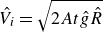 $\hat {V}_i = \sqrt {2 At \hat g \hat R}$
. This scaling provides a useful approximation of front propagation. Building on this framework, Séon et al. (Reference Séon, Hulin, Salin, Perrin and Hinch2005) showed that front velocities
$\hat {V}_i = \sqrt {2 At \hat g \hat R}$
. This scaling provides a useful approximation of front propagation. Building on this framework, Séon et al. (Reference Séon, Hulin, Salin, Perrin and Hinch2005) showed that front velocities $V_{\!f}$
, of Newtonian–Newtonian exchange flow in a pipe, increased with
$V_{\!f}$
, of Newtonian–Newtonian exchange flow in a pipe, increased with $\beta$
to a plateau:
$\beta$
to a plateau: $\hat V_{\!f}=0.7 \sqrt {2 At \hat g \hat R}$
, for
$\hat V_{\!f}=0.7 \sqrt {2 At \hat g \hat R}$
, for $65^{\circ }\lt \beta \lt 82^{\circ }$
.
$65^{\circ }\lt \beta \lt 82^{\circ }$
.
To understand the internal mechanics driving these front velocities, figure 22 presents the axial velocity profiles across the pipe diameter at $z=80$
, obtained purely from our numerical simulations under different flow conditions. In figure 22(a), the effect of pipe inclination is shown. For the vertical configuration (
$z=80$
, obtained purely from our numerical simulations under different flow conditions. In figure 22(a), the effect of pipe inclination is shown. For the vertical configuration ( $\beta =0^\circ$
, blue line), the upward-moving Newtonian finger remains centred, exhibiting a Poiseuille-like velocity distribution, while the downward-moving viscoplastic fluid (negative
$\beta =0^\circ$
, blue line), the upward-moving Newtonian finger remains centred, exhibiting a Poiseuille-like velocity distribution, while the downward-moving viscoplastic fluid (negative $U_z$
) displays a plug-like profile (flattened plug region identified by arrows) across the pipe cross-section except close to the walls and centre of the pipe where it is yielded due to the higher applied shear and interfacial stresses. When the inclination increases to
$U_z$
) displays a plug-like profile (flattened plug region identified by arrows) across the pipe cross-section except close to the walls and centre of the pipe where it is yielded due to the higher applied shear and interfacial stresses. When the inclination increases to $\beta =15^\circ$
(red line), the velocity distribution becomes asymmetric: the Newtonian phase accelerates preferentially along one side of the pipe while the viscoplastic phase is displaced non-uniformly on the opposite side. At higher inclination (
$\beta =15^\circ$
(red line), the velocity distribution becomes asymmetric: the Newtonian phase accelerates preferentially along one side of the pipe while the viscoplastic phase is displaced non-uniformly on the opposite side. At higher inclination ( $\beta =30^\circ$
, green line), this asymmetry intensifies, with the Newtonian upward flow confined near one pipe wall and the flattened plug region of the viscoplastic downward motion concentrated towards the centre of the pipe.
$\beta =30^\circ$
, green line), this asymmetry intensifies, with the Newtonian upward flow confined near one pipe wall and the flattened plug region of the viscoplastic downward motion concentrated towards the centre of the pipe.
Axial velocity profiles across the pipe diameter at $z=80$
for (a) different inclination angles
$z=80$
for (a) different inclination angles $\beta =0^\circ$
(blue),
$\beta =0^\circ$
(blue), $\beta =15^\circ$
(red) and
$\beta =15^\circ$
(red) and $\beta ={30}^\circ$
(green) for
$\beta ={30}^\circ$
(green) for $\chi =9.75$
and
$\chi =9.75$
and $Y=0.022$
, (b) different yield stresses quantified by
$Y=0.022$
, (b) different yield stresses quantified by $Y=[0.003, 0.02, 0.036]$
at
$Y=[0.003, 0.02, 0.036]$
at $\beta =15^\circ$
and (c) different density differences quantified by
$\beta =15^\circ$
and (c) different density differences quantified by $\chi =[9.72, 13.73, 18.47]$
at
$\chi =[9.72, 13.73, 18.47]$
at $\beta =15^\circ$
. The colour intensity of the lines in (b,c) represents the values of
$\beta =15^\circ$
. The colour intensity of the lines in (b,c) represents the values of $Y$
and
$Y$
and $\chi$
, respectively; i.e. a darker line represents a higher
$\chi$
, respectively; i.e. a darker line represents a higher $Y$
in (b) and a greater
$Y$
in (b) and a greater $\chi$
in (c). Arrows show the extent of plug regions.
$\chi$
in (c). Arrows show the extent of plug regions.

Figure 22(b) illustrates the influence of yield stress at $\beta =15^\circ$
. Lower yield-stress values (lighter lines) lead to a more fluid-like behaviour of the viscoplastic phase, resulting in stronger downward shear-driven velocities. As the yield stress increases (darker lines), the viscoplastic fluid resists deformation, and the velocity distribution flattens, characteristic of plug flow. Figure 22(c) highlights the effect of density differences at
$\beta =15^\circ$
. Lower yield-stress values (lighter lines) lead to a more fluid-like behaviour of the viscoplastic phase, resulting in stronger downward shear-driven velocities. As the yield stress increases (darker lines), the viscoplastic fluid resists deformation, and the velocity distribution flattens, characteristic of plug flow. Figure 22(c) highlights the effect of density differences at $\beta =15^\circ$
. A smaller density contrast (lighter lines) yields more balanced counterflow between phases, while larger density differences (darker lines) enhance buoyancy-driven segregation, leading to greater velocity asymmetry and intensified fingering. These findings are consistent with earlier observations on buoyancy-driven instabilities in multiphase displacement flows (Dai et al. Reference Dai, Eslami, Schneider, Liu and Schwering2024).
$\beta =15^\circ$
. A smaller density contrast (lighter lines) yields more balanced counterflow between phases, while larger density differences (darker lines) enhance buoyancy-driven segregation, leading to greater velocity asymmetry and intensified fingering. These findings are consistent with earlier observations on buoyancy-driven instabilities in multiphase displacement flows (Dai et al. Reference Dai, Eslami, Schneider, Liu and Schwering2024).
In figure 22, the location of the zero velocity ( $U_z=0$
) changes systematically with the flow parameters and therefore serves as an indication of the fluid–fluid interface. In figure 22(a), the profiles at
$U_z=0$
) changes systematically with the flow parameters and therefore serves as an indication of the fluid–fluid interface. In figure 22(a), the profiles at $\beta =0^\circ$
exhibit two
$\beta =0^\circ$
exhibit two $U_z=0$
points located near the lateral walls, whereas at
$U_z=0$
points located near the lateral walls, whereas at $\beta =15^\circ$
these points migrate towards one side, evidencing interface displacement and flow asymmetry induced by the pipe tilt. In figure 22(b), increasing
$\beta =15^\circ$
these points migrate towards one side, evidencing interface displacement and flow asymmetry induced by the pipe tilt. In figure 22(b), increasing $Y$
shifts the zero-velocity location(s) closer to the wall: for low
$Y$
shifts the zero-velocity location(s) closer to the wall: for low $Y$
a single crossing is observed at the middle of the pipe, while at the largest
$Y$
a single crossing is observed at the middle of the pipe, while at the largest $Y$
an additional zero-velocity point appears adjacent to the wall, consistent with a thicker plug region and a narrowed shear zone. In figure 22(c), increasing
$Y$
an additional zero-velocity point appears adjacent to the wall, consistent with a thicker plug region and a narrowed shear zone. In figure 22(c), increasing $\chi$
initially displaces the zero-velocity point towards the less dense fluid, reflecting buoyancy-driven stratification of the interface. The zero-velocity position then remains unchanged for further increases in
$\chi$
initially displaces the zero-velocity point towards the less dense fluid, reflecting buoyancy-driven stratification of the interface. The zero-velocity position then remains unchanged for further increases in $\chi$
. This is not coincidental, but rather indicates that the flow has reached an asymptotic strongly segregated regime. At high
$\chi$
. This is not coincidental, but rather indicates that the flow has reached an asymptotic strongly segregated regime. At high $\chi$
, the transverse location of the interface becomes geometrically locked by the global zero-net-volumetric-flux constraint of the closed pipe (
$\chi$
, the transverse location of the interface becomes geometrically locked by the global zero-net-volumetric-flux constraint of the closed pipe ( $Q_H + Q_L = 0$
). Consequently, while the velocity profile extrema (maximum and minimum values) continue to scale up with the buoyant driving force, the interface location is stabilised, and the shear distribution and flow intensity within each fluid layer are still affected by the density contrast.
$Q_H + Q_L = 0$
). Consequently, while the velocity profile extrema (maximum and minimum values) continue to scale up with the buoyant driving force, the interface location is stabilised, and the shear distribution and flow intensity within each fluid layer are still affected by the density contrast.
3.6. Dynamics of viscoplastic flow below the gate valve
Figure 23 presents the dynamics of the more dense viscoplastic fluid released upon opening the gate valve into the lower half of the pipe initially filled with dyed Newtonian fluid. Since the Newtonian phase is dyed for contrast, the invading viscoplastic fluid itself is not directly visible; instead, the flow evolution is visualised through colour-coded concentration snapshots, as shown in figure 23( $a_1$
,
$a_1$
, $a_2$
), where lighter colours denote regions of lower Newtonian-fluid concentration. In the vertical configuration (
$a_2$
), where lighter colours denote regions of lower Newtonian-fluid concentration. In the vertical configuration ( $\beta =0^\circ$
), the viscoplastic phase exhibits a dripping-like motion, where buoyancy forces act to detach small viscoplastic fluid chunks that fall intermittently along the pipe. This fragmented descent is characteristic of yield-stress fluids within confined geometries, in which the fluid resists deformation until local stresses exceed the yield threshold, at which point small packets of fluid break up and descend. The spatiotemporal map (figure 23
$\beta =0^\circ$
), the viscoplastic phase exhibits a dripping-like motion, where buoyancy forces act to detach small viscoplastic fluid chunks that fall intermittently along the pipe. This fragmented descent is characteristic of yield-stress fluids within confined geometries, in which the fluid resists deformation until local stresses exceed the yield threshold, at which point small packets of fluid break up and descend. The spatiotemporal map (figure 23 $b_1$
) highlights this process, with discontinuous and step-like fronts (light-coloured downward streaks) associated with successive detachments.
$b_1$
) highlights this process, with discontinuous and step-like fronts (light-coloured downward streaks) associated with successive detachments.
(a $_1$
,a
$_1$
,a $_2$
) Sequence of experimental snapshots of the flow below the gate valve for sample IX,
$_2$
) Sequence of experimental snapshots of the flow below the gate valve for sample IX, $\chi =9.75$
and
$\chi =9.75$
and $Y=0.022$
; the dimensionless field of view is
$Y=0.022$
; the dimensionless field of view is $2 \times 150$
. (a
$2 \times 150$
. (a $_1$
)
$_1$
) $\beta =0^\circ$
; from left to right,
$\beta =0^\circ$
; from left to right, $t=$
[20:125:1700]. (a
$t=$
[20:125:1700]. (a $_2$
)
$_2$
) $\beta =30^\circ$
; from left to right,
$\beta =30^\circ$
; from left to right, $t=$
[10:90:1300]. (b
$t=$
[10:90:1300]. (b $_1$
,b
$_1$
,b $_2$
) The spatiotemporal diagram of the normalised depth-averaged concentration field,
$_2$
) The spatiotemporal diagram of the normalised depth-averaged concentration field, $\bar {\bar {c}}({z},t)$
, corresponding to (a
$\bar {\bar {c}}({z},t)$
, corresponding to (a $_1$
,a
$_1$
,a $_2$
), respectively.
$_2$
), respectively.

When the pipe is inclined at $\beta =30^\circ$
, the flow mechanism changes substantially due to the combined effects of gravity and wall interaction. In this case, the viscoplastic fluid preferentially adheres to and descends along the lower wall, forming larger coherent masses rather than small dripping droplets. The yield stress promotes cohesive motion, while the inclined geometry enhances gravitational spreading along the boundary, resulting in a more continuous displacement. It can also be seen that the falling viscoplastic chunks become larger with the passage of time. The spatiotemporal diagram (figure 23
$\beta =30^\circ$
, the flow mechanism changes substantially due to the combined effects of gravity and wall interaction. In this case, the viscoplastic fluid preferentially adheres to and descends along the lower wall, forming larger coherent masses rather than small dripping droplets. The yield stress promotes cohesive motion, while the inclined geometry enhances gravitational spreading along the boundary, resulting in a more continuous displacement. It can also be seen that the falling viscoplastic chunks become larger with the passage of time. The spatiotemporal diagram (figure 23 $b_2$
) supports this interpretation, with smoother, slanted concentration bands that indicate the sustained descent of large fluid portions. At longer times (
$b_2$
) supports this interpretation, with smoother, slanted concentration bands that indicate the sustained descent of large fluid portions. At longer times ( $t\gt 900$
), the bottom of the pipe is full of viscoplastic fluid, indicated by the white region in figure 23
$t\gt 900$
), the bottom of the pipe is full of viscoplastic fluid, indicated by the white region in figure 23 $(b_2)$
. This contrast between vertical and inclined configurations underscores the strong sensitivity of viscoplastic displacement to system orientation: while vertical flows are governed by localised yielding and droplet detachment, inclined flows promote wall-guided cohesive transport, leading to more effective replacement of the less dense phase.
$(b_2)$
. This contrast between vertical and inclined configurations underscores the strong sensitivity of viscoplastic displacement to system orientation: while vertical flows are governed by localised yielding and droplet detachment, inclined flows promote wall-guided cohesive transport, leading to more effective replacement of the less dense phase.
Figure 24 quantifies the settling dynamics of the viscoplastic fluid fragments released below the gate valve. The settling velocity is extracted from the spatiotemporal diagram (e.g. figure 23 $b_1$
,
$b_1$
, $b_2$
) by fitting straight lines to the distinct descending streaks and averaging the slopes (
$b_2$
) by fitting straight lines to the distinct descending streaks and averaging the slopes ( $\Delta z / \Delta t$
) across multiple representative fluid fragments. This figure presents the dimensionless settling velocity,
$\Delta z / \Delta t$
) across multiple representative fluid fragments. This figure presents the dimensionless settling velocity, $V_s$
, plotted against the buoyancy number,
$V_s$
, plotted against the buoyancy number, $\chi$
. Despite variations in inclination and yield stress, the majority of the data cluster around a nearly constant value of
$\chi$
. Despite variations in inclination and yield stress, the majority of the data cluster around a nearly constant value of $V_s \approx 0.65$
, as marked by the dotted line. This collapse of the data implies that, once normalised by the buoyancy-driven scaling, the settling velocity becomes largely independent of the system parameters. Such a result highlights the influence of buoyancy in controlling descent, with wall inclination and yield effects primarily modulating the fragmentation process rather than the normalised settling rate itself. Overall, these findings demonstrate that while the absolute settling velocity depends strongly on buoyancy, the dimensionless dynamics exhibits a universal character.
$V_s \approx 0.65$
, as marked by the dotted line. This collapse of the data implies that, once normalised by the buoyancy-driven scaling, the settling velocity becomes largely independent of the system parameters. Such a result highlights the influence of buoyancy in controlling descent, with wall inclination and yield effects primarily modulating the fragmentation process rather than the normalised settling rate itself. Overall, these findings demonstrate that while the absolute settling velocity depends strongly on buoyancy, the dimensionless dynamics exhibits a universal character.
Dimensionless settling velocity versus longitudinal buoyancy $\chi \cos \beta$
. The size and colour of symbols represent
$\chi \cos \beta$
. The size and colour of symbols represent $\beta$
and
$\beta$
and $Y$
, respectively. The dotted line marks
$Y$
, respectively. The dotted line marks $V_s\approx 0.65$
.
$V_s\approx 0.65$
.

4. Summary
Motivated by the P&A process in oil and gas wells, we have investigated the placement of a more dense viscoplastic fluid on top of a less dense Newtonian fluid in an inclined pipe, via experiments and numerical simulations. The fluids are miscible with a relatively small density difference. Our experimental approach includes a non-intrusive experimental technique, i.e. camera imaging. Our dimensional analysis has revealed that the main dimensionless numbers are the buoyancy number ( $\chi$
), the yield number (
$\chi$
), the yield number ( $Y$
) and the inclination angle (
$Y$
) and the inclination angle ( $\beta$
). We have studied the effects of these dimensionless numbers on the concentration and velocity fields, the front velocities and yielded and unyielded zones. Complementary simulations were run in the limit of high Péclet number using OpenFOAM to elucidate the effects of the parameters on the flow dynamics, i.e. a feature that cannot be easily captured in our experiments.
$\beta$
). We have studied the effects of these dimensionless numbers on the concentration and velocity fields, the front velocities and yielded and unyielded zones. Complementary simulations were run in the limit of high Péclet number using OpenFOAM to elucidate the effects of the parameters on the flow dynamics, i.e. a feature that cannot be easily captured in our experiments.
Our analysis of the top half of the pipe showed two distinct regimes, i.e. fingering and slumping. In the fingering regime, we have categorised flows as helical finger, disconnected finger and slug flows. We have analysed this regime in terms of the length and time scale of finger separation, maximum stable length of the finger, finger length variation from its separation point to the pipe end and wavelength of the helical flow patterns behind the finger. Regarding the slumping regime, we have numerically considered the deviation of the finger tip from axisymmetry versus the inclination angle. Quantitative analysis shows that finger eccentricity ( $e$
) grows markedly with inclination, from negligible values at
$e$
) grows markedly with inclination, from negligible values at $\beta \le 10^\circ$
to
$\beta \le 10^\circ$
to $e \approx 0.11$
at
$e \approx 0.11$
at $\beta = 15^\circ$
, peaking at
$\beta = 15^\circ$
, peaking at $e \approx 0.23$
at
$e \approx 0.23$
at $\beta = 45^\circ$
. This nonlinear progression suggests a threshold behaviour, where small inclinations have a limited effect, but moderate-to-high inclinations strongly bias the finger towards the lower side of the pipe.
$\beta = 45^\circ$
. This nonlinear progression suggests a threshold behaviour, where small inclinations have a limited effect, but moderate-to-high inclinations strongly bias the finger towards the lower side of the pipe.
Analysis of interface height profiles in an inclined configuration showed minimal oscillations near the fluid front, with stronger disturbances developing farther downstream. Testing various moving reference frames reveals that only the frame moving with the front, $z - V_{\!f} t$
, yields self-similar interface profiles, indicating a steady travelling Newtonian finger front as the dominant interfacial structure. Instabilities become observable only a significant distance behind the advancing front, which could result from slow growth of a convective interfacial instability controlled by the large viscosity of the viscoplastic layer. Numerical solutions show that the flow within the Newtonian finger far behind the front can be significantly faster than the front speed, producing an influx that the front can only absorb up to a point. Consequently, this deceleration of the Newtonian fluid stream may be the cause of interfacial perturbations. The numerical results also show the presence of an unyielded sheath of fluid around the interface for the stable part of advancing fingers.
$z - V_{\!f} t$
, yields self-similar interface profiles, indicating a steady travelling Newtonian finger front as the dominant interfacial structure. Instabilities become observable only a significant distance behind the advancing front, which could result from slow growth of a convective interfacial instability controlled by the large viscosity of the viscoplastic layer. Numerical solutions show that the flow within the Newtonian finger far behind the front can be significantly faster than the front speed, producing an influx that the front can only absorb up to a point. Consequently, this deceleration of the Newtonian fluid stream may be the cause of interfacial perturbations. The numerical results also show the presence of an unyielded sheath of fluid around the interface for the stable part of advancing fingers.
Analysis of the lower half of the pipe showed that the viscoplastic fluid descends as separated segments, whose size increases with pipe inclination. The dynamics of the less dense fluid front in the upper half and the settling velocity of the viscoplastic segments in the lower half indicate that the former is primarily governed by the buoyancy number, while the latter follows a buoyancy–inertia scaling, with an empirical correlation accurately capturing the downward velocities.
From an industrial perspective, these results provide insight into the challenges of off-bottom plug placement in well casings. Unlike primary cementing operations, where complete displacement of the in situ fluid (spacer or mud) is desired, in plug placement, the ideal is to suppress flow altogether, such that the Newtonian fluid does not migrate significantly once the cement slurry is placed. Our results show that well inclination, slurry yield stress and density contrast exert a strong influence on the persistence of motion. In inclined wellbores (commonly referred to in industry as deviated wells), inclination-driven asymmetry increases the risk of Newtonian fluid channelling and macroscopic buoyancy-driven fluid exchange (recirculation), which compromises the stability of the plug. Similarly, tuning of the slurry yield stress may permit undesirable fingering if too low. Excessive density contrast can also enhance buoyancy-driven segregation, leading to upward migration of the Newtonian phase as a finger in vertical configuration, in which shorter fingers and longer detachment times are preferred: shorter fingers minimise the amount of water entering the cement slurry above, while longer rise times allow the cement to thicken sufficiently before finger development, thereby preserving the structural integrity of the cement. Aside from estimating water volumes in the detached finger/slug, it is of interest to understand evolution of the mixed-zone structure and to what an extent this limits the later exchange flow. Therefore, for reliable off-bottom plug placement, it is essential to engineer cement slurries with tailored rheological properties and carefully controlled density contrasts to minimise post-placement flow. Our results and discussion in § 3.1 address the difficulty of making design predictions.
Our results also suggest that, below the placed cement plug, detachment and settling of cement slurry fragments may occur. This might eventually compromise plug stability above, although the long lengths of typical cement plugs would make this less likely. The upper plug itself (our observations of behaviour in the upper section) and exchange flow with the water are most relevant for controlling fragment motion. Understanding how settling velocity scales with buoyancy and yield stress provides a basis for designing cement formulations and operational conditions that limit undesired fragment movement in critical regions. The results of this study allow engineers and researchers to better comprehend the complex fluid placement flows that occur, particularly in P&A cementing operations of oil and gas wells.
Finally, it is important to acknowledge that the regime diagrams and empirical correlations presented in this study exhibit a degree of natural scatter. This variability stems from two primary sources. First, to systematically analyse the dominant flow physics, we projected a highly complex parameter space (comprising at least eight dimensionless groups, as outlined in table 3) onto the three most critical macroscopic variables: $Y$
,
$Y$
, $\chi$
and
$\chi$
and $\beta$
. Minor variations in the secondary parameters across the experimental matrix inevitably introduce spread when collapsed onto these primary axes. Second, yield-stress fluids are highly sensitive to initial conditions. The initial structural perturbation induced by the mechanical opening of the gate valve creates a complex transient interface that naturally varies slightly between runs, directly influencing the local stress concentrations and the precise onset of instability. Consequently, the empirical correlations and boundaries provided here should not be viewed as absolute deterministic limits, but rather as conservative operational envelopes. From an industrial perspective, this scatter reflects the physical realities and uncertainties of actual P&A operations. Future work, potentially leveraging fully resolved 3-D transient simulations of the placement process, will be required to further disentangle the effects of secondary dimensionless groups and initial perturbations.
$\beta$
. Minor variations in the secondary parameters across the experimental matrix inevitably introduce spread when collapsed onto these primary axes. Second, yield-stress fluids are highly sensitive to initial conditions. The initial structural perturbation induced by the mechanical opening of the gate valve creates a complex transient interface that naturally varies slightly between runs, directly influencing the local stress concentrations and the precise onset of instability. Consequently, the empirical correlations and boundaries provided here should not be viewed as absolute deterministic limits, but rather as conservative operational envelopes. From an industrial perspective, this scatter reflects the physical realities and uncertainties of actual P&A operations. Future work, potentially leveraging fully resolved 3-D transient simulations of the placement process, will be required to further disentangle the effects of secondary dimensionless groups and initial perturbations.
Acknowledgements
We gratefully acknowledge the financial support provided by NSERC and PTAC (project numbers ALLRP 577111-2022 and AUPRF2022-000124, respectively). We thank the Digital Research Alliance of Canada, supporting us in high-performance computing and parallel processing. Use of grammar/language tools for improving text readability is also acknowledged.
Declaration of interests
The authors report no conflict of interest.
Data availability statement
The data that support the findings of this study are available within the article.


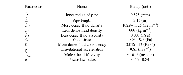
 ⋅^
⋅^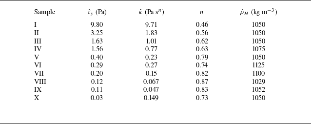

 γ
γ ≈
≈ G′
G′ G″
G″ τ^
τ^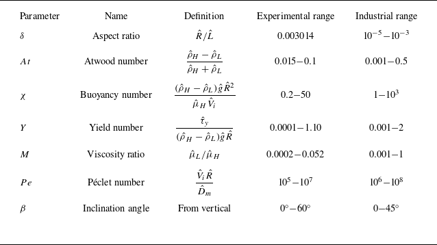

 χ=7.98
 Y=0.04
 β=0∘
β=0∘ t=27
t=27
 χ=7.98
 Y=0.04
 β=0∘
β=0∘ t=340
t=340 β=15∘
β=15∘ t=310
t=310 2×50
2×50 z−y
z−y x=
x= β
β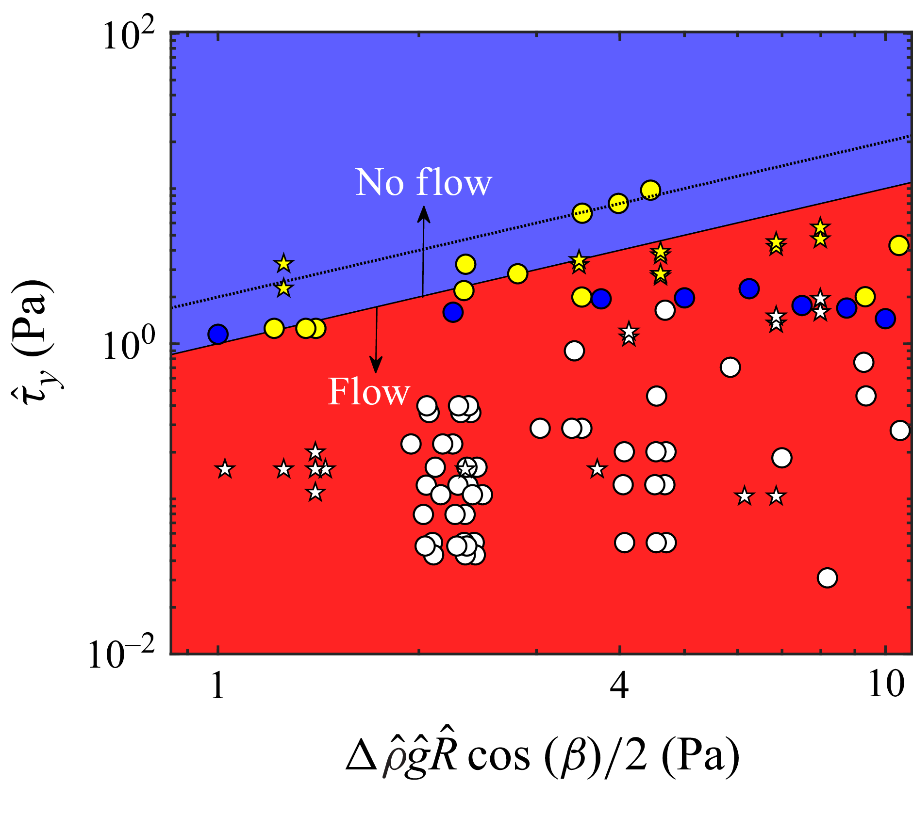
 τ^y=0.5Δρ^g^R^cosβ
 Y=0.5cosβ
 Y=cosβ
 τ^y=Δρ^g^R^cosβ
 χ=2.05
 Y=0.082
 β=0∘
β=0∘ t=[390,940,1364,2070,2834,3366]
 χ=6.98
 Y=0.022
 β=30∘
β=30∘ t=[297,416,559,702,880,1011]
 2×150
2×150
 c¯¯(z,t)
 χ=7.98
 Y=0.022
 β=0∘
β=0∘ z=8
z=8 2×120
2×120
 χ=7.98
 Y=0.022
 β=15∘
β=15∘ z=8
z=8 2×120
2×120
 χ=0.20
 Y=0.34
 t=[135,434,710,1064,1450,2010]
 χ=1.2
χ=1.2 Y=0.082
 t=[181,283,370,507,667,1051]
 χ=10.46
 Y=0.0063
 t=[51,143,180,257,337,481]
 β=0∘
β=0∘ 2×150
2×150
 c¯¯(z,t)
 Vf
Vf l^f,i
l^f,i l^f,e
l^f,e
 χ
χ χ
χ Y
Y ⧫
⧫ ▸
▸ ∙
∙
 ls
ls χ
χ ls=(37±5)χ−0.5
 ts
ts χ
χ ts=(1951±320)χ−0.5
 Y
Y
 l^f,i
l^f,i l^f,e
l^f,e lf,i
lf,i lf,e
lf,e Y
Y χ
χ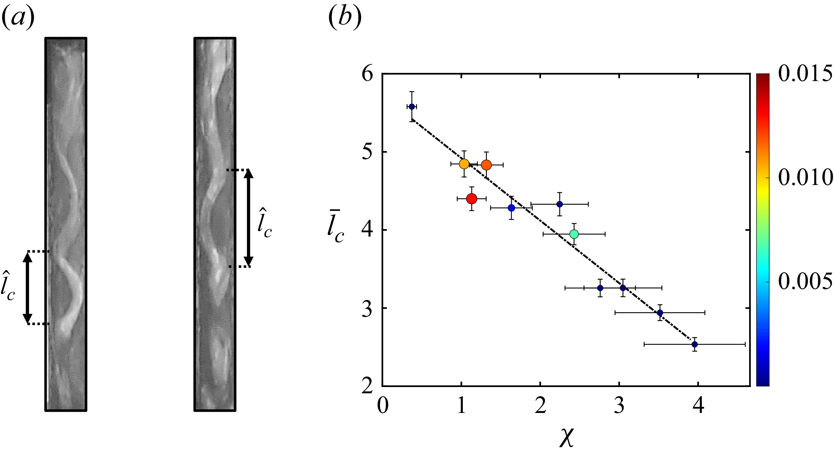
 χ=3.26
 χ=1.78
 lc
lc χ
χ lc=5.72−0.27χ
 Y
Y
 χ=9.73
 Y=0.022
 β=15∘
β=15∘ t=[58,139,216,420,604,710]
 β=30∘
β=30∘ t=[34,120,205,390,505,602]
 c¯¯(z,t)
 e
e β
β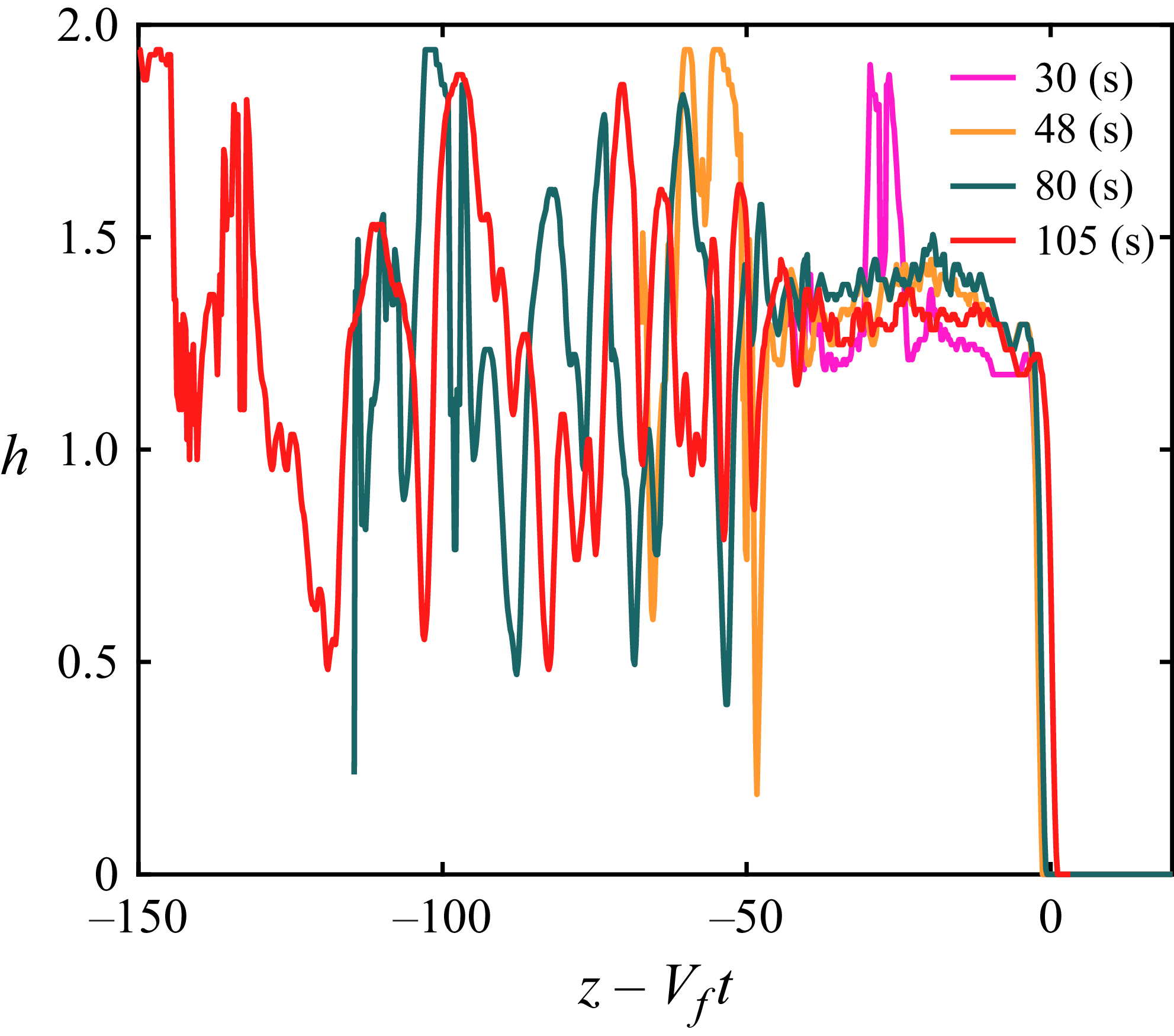
 h
h t=[30,48,80,105]
 β=30∘
β=30∘ χ=9.75
 Y=0.022
 z−Vft
z−Vft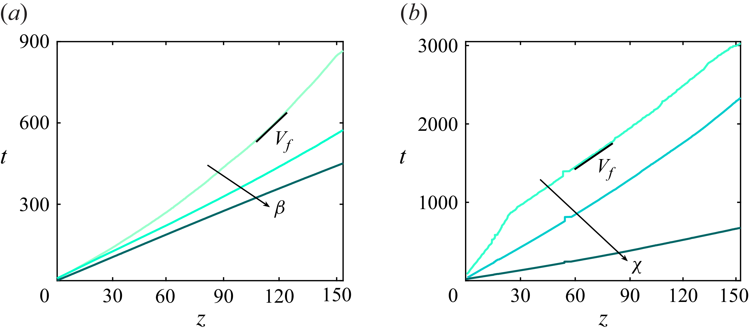
 z
z χ=9.75
 Y=0.022
 β=0∘, 15∘, 30∘
 χ
χ β=0∘
β=0∘ χ=0.20,3.56,6.74
 Y=0.50,0.013,0.0003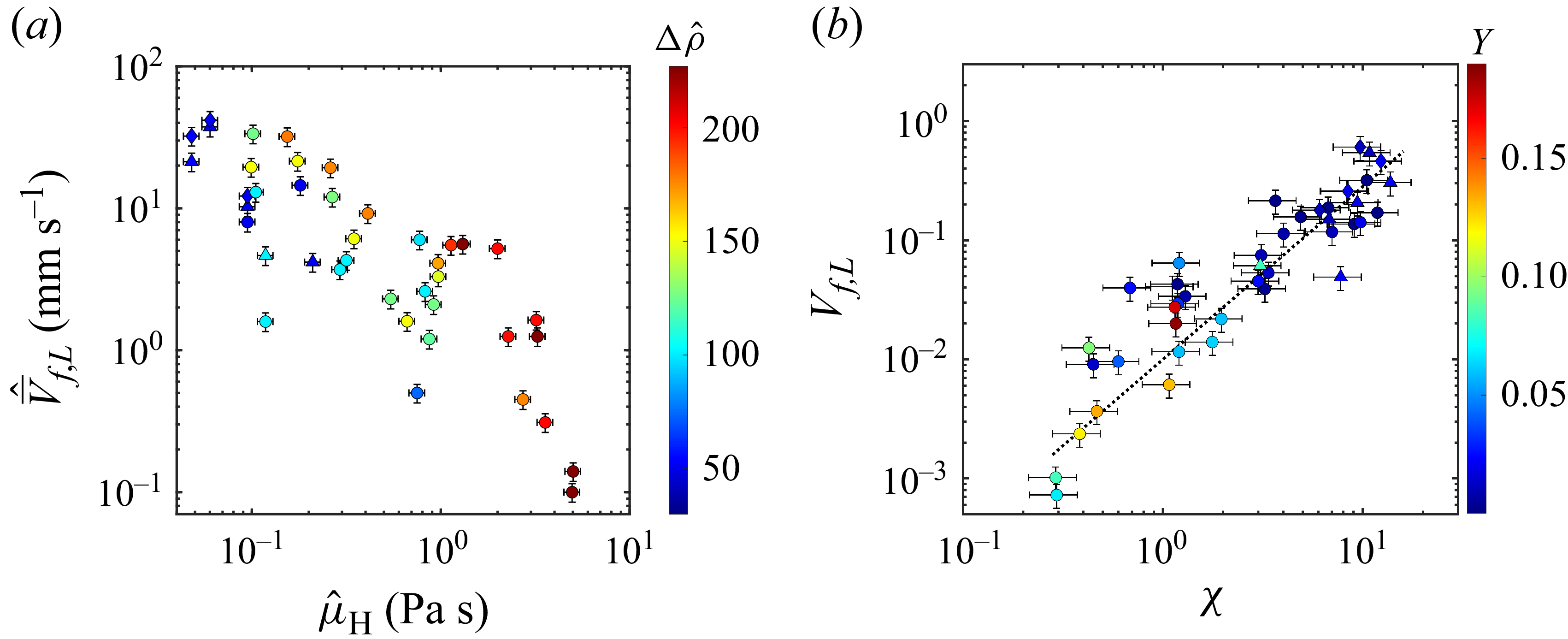
 V¯^f,L
 μ^H
μ^H Δρ^=ρ^H−ρ^L
 V¯f,L
V¯f,L χcosβ
χcosβ V¯f=0.01(χcosβ)1.45
 Y
Y β=0∘
β=0∘ ∙
∙ β=15∘
β=15∘ ▴
▴ β=30∘
β=30∘ ⧫
⧫
 z=80
z=80 β=0∘
β=0∘ β=15∘
β=15∘ β=30∘
β=30∘ χ=9.75
 Y=0.022
 Y=[0.003,0.02,0.036]
 β=15∘
β=15∘ χ=[9.72,13.73,18.47]
 β=15∘
β=15∘ Y
Y χ
χ Y
Y χ
χ
 1
1 2
2 χ=9.75
 Y=0.022
 2×150
2×150 1
1 β=0∘
β=0∘ t=
t= 2
2 β=30∘
β=30∘ t=
t= 1
1 2
2 c¯¯(z,t)
 1
1 2
2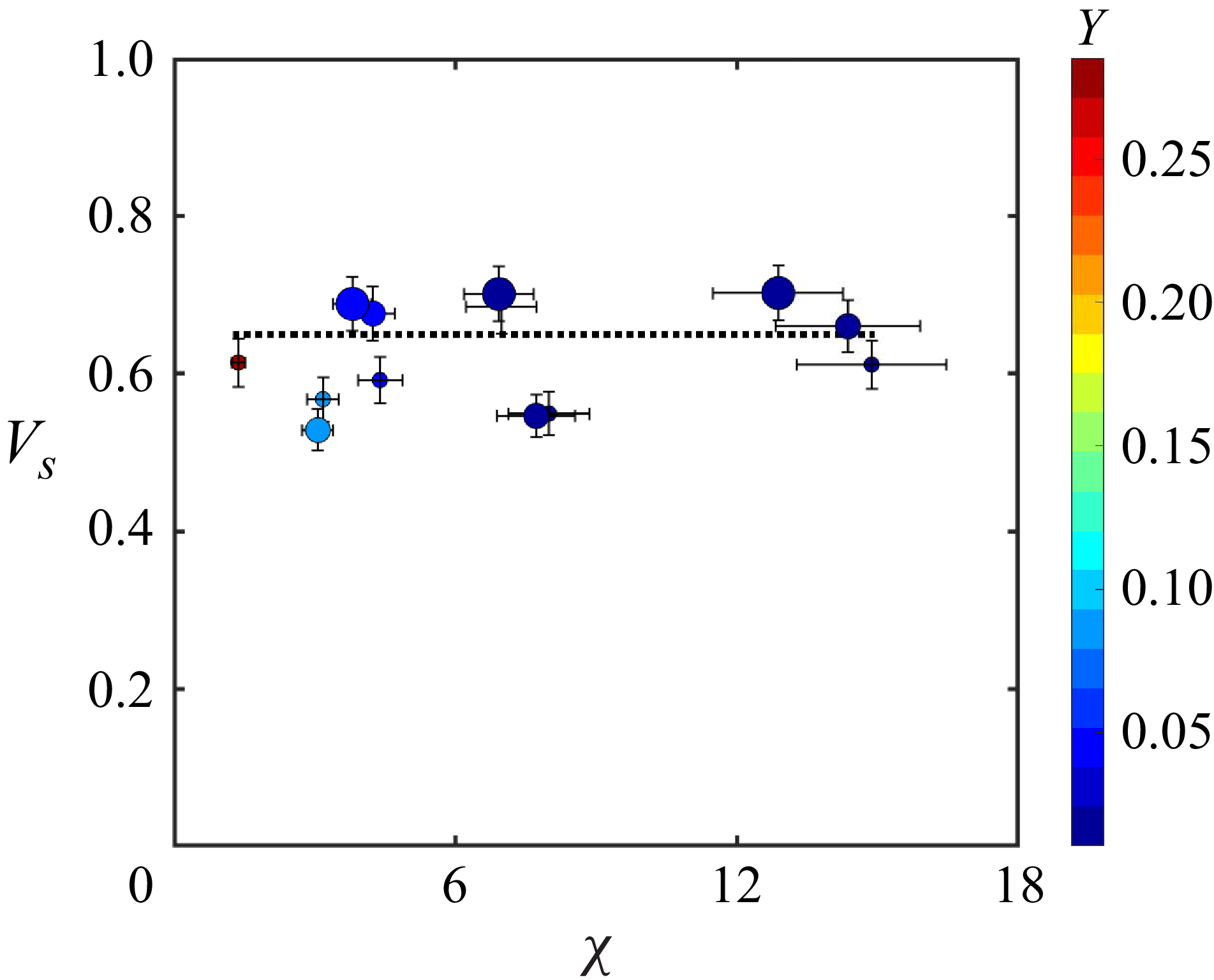
 χcosβ
χcosβ β
β Y
Y Vs≈0.65
 Open access

