


1. Introduction
Bubbles are ubiquitous in diverse fluid mediums, including water, oils, bodily fluids, beverages and chemical reagents, such as large-scale oceanic bubbles (De Graaf, Brandner & Penesis Reference De Graaf, Brandner and Penesis2014; Li et al. Reference Li, van der Meer, Zhang, Prosperetti and Lohse2020) and drag-reducing bubbles (Verschoof et al. Reference Verschoof, Van Der, R., Sun and Lohse2016), biological phenomena (Lohse, Schmitz & Versluis Reference Lohse, Schmitz and Versluis2001), explosion bubbles (Best Reference Best1991), vapour bubbles in boiling oil (Mitrovic Reference Mitrovic1998; Lioumbas & Karapantsios Reference Lioumbas and Karapantsios2015), micro-vacuoles in tissues (Fry et al. Reference Fry, Sanghvi, Foster, Bihrle and Hennige1995; Klibanov Reference Klibanov2007), pressurised bubbles in carbonated drinks (Vega-Martínez et al. Reference Vega-Martínez, Enríquez and Rodríguez-Rodríguez2017; Zenit & Rodríguez-Rodríguez Reference Zenit and Rodríguez-Rodríguez2018), and bubbles from chemical reactions (Merouani & Hamdaoui Reference Merouani and Hamdaoui2016; Sabdenov Reference Sabdenov2020). Across these applications, fluid compressibility and viscosity critically influence bubble dynamics by dissipating energy within the bubble system (Wang Reference Wang2016; Fang et al. Reference Fang, Wang, Meng, Ming and Zhang2025a , Reference Fang, Wang, Meng, Ming and Zhangb ). To elucidate these mechanisms and explore how fluid properties affect bubble behaviour, extensive research has employed a number of theoretical analysis, which has been instrumental in formalising the underlying mechanical principles mathematically.
Theoretical investigations of bubble dynamics have evolved significantly over decades. Assuming incompressible fluids, early foundational work established classical models primarily through modifications of the Rayleigh–Plesset equation (Rayleigh Reference Rayleigh1917; Plesset Reference Plesset1949), focusing heavily on viscosity effects for bubble oscillation (Plesset Reference Plesset1964; Yang & Yeh Reference Yang and Yeh1966; Fogler Reference Fogler1969; Apfel Reference Apfel1981). Subsequently, models were progressively extended to encompass compressible fluids (Gilmore Reference Gilmore1952; Keller & Miksis Reference Keller and Miksis1980; Ma, Hsiao & Chahine Reference Ma, Hsiao and Chahine2018). More recently, Zhang et al. (Reference Zhang, Li, Xu, Pei, Li and Liu2024) proposed bubble oscillation and migration equations (the Zhang equation) from a potential flow perspective, establishing a multi-factor theoretical model for spherical bubbles. While the Zhang equation incorporates viscosity considerations for bubble migration, its viscous effect is represented through an added drag coefficient ( ${C_d}$
). This approach highlights a persistent challenge: many hydrodynamic models based on potential flow theory (Hicks Reference Hicks1970; Plesset & Prosperetti Reference Plesset and Prosperetti1977; Prosperetti & Lezzi Reference Prosperetti and Lezzi1986; Brujan, Pearson & Blake Reference Brujan, Pearson and Blake2005; Peñas-López et al. Reference Peñas-López, Parrales, Rodríguez-Rodríguez and van der Meer2016) inherently struggle to objectively characterise fluid viscosity, necessitating empirical adjustments via drag coefficients. This reliance on phenomenological parametrisation introduces empirical uncertainties, potentially hindering rigorous theoretical exploration of the coupling between bubble oscillation and migration dynamics.
${C_d}$
). This approach highlights a persistent challenge: many hydrodynamic models based on potential flow theory (Hicks Reference Hicks1970; Plesset & Prosperetti Reference Plesset and Prosperetti1977; Prosperetti & Lezzi Reference Prosperetti and Lezzi1986; Brujan, Pearson & Blake Reference Brujan, Pearson and Blake2005; Peñas-López et al. Reference Peñas-López, Parrales, Rodríguez-Rodríguez and van der Meer2016) inherently struggle to objectively characterise fluid viscosity, necessitating empirical adjustments via drag coefficients. This reliance on phenomenological parametrisation introduces empirical uncertainties, potentially hindering rigorous theoretical exploration of the coupling between bubble oscillation and migration dynamics.
The characterisation of drag coefficients, crucial in migration models, has its own theoretical trajectory. For flow past spherical structures, Aybers & Tapucu (Reference Aybers and Tapucu1969) noted that Stokes originally elucidated low-Reynolds-number drag, where a bubble’s surface tangential velocity equals half that of a rigid sphere, yielding a viscous drag coefficient of unity under Stokes’ assumptions. Later boundary layer analyses for higher Reynolds numbers by Levich (Reference Levich1962) and Moore (Reference Moore1963) aligned with this, deriving ${C}_{{d}}=48/\textit{Re}$
. However, fundamental limitations arise from the Stokes hypothesis neglecting convective terms, intrinsic constraints of boundary layer theory, and omission of higher-order terms. These simplifications lead to significant discrepancies in applicability and accuracy for drag coefficient implementations, preventing a novel theoretical framework. Furthermore, the migration equation formulations in these studies omitted critical fluid compressibility effects and employed time-independent drag coefficients lacking analytical expressions. Consequently, while partially elucidating parametric dependencies under constrained conditions, these models cannot universally describe diverse bubble behaviours. Numerous other studies have analysed drag in bubbles under various conditions (Roghair et al. Reference Roghair, Lau, Deen, Slagter, Baltussen, Annaland and Kuipers2011; Mattson & Mahesh Reference Mattson and Mahesh2011; Ravelet, Colin & Risso Reference Ravelet, Colin and Risso2011; Roig et al. Reference Roig, Roudet, Risso and Billet2012; Brujan et al. Reference Brujan, Zhang, Liu, Ogasawara and Takahira2022), offering more intuitive and accurate depictions. However, these investigations rely heavily on numerical computation and experimental observation, limiting their direct utility for theoretical development and subsequent research. Moreover, numerical results depend critically on computational precision, and exploring underlying principles demands substantial investment.
${C}_{{d}}=48/\textit{Re}$
. However, fundamental limitations arise from the Stokes hypothesis neglecting convective terms, intrinsic constraints of boundary layer theory, and omission of higher-order terms. These simplifications lead to significant discrepancies in applicability and accuracy for drag coefficient implementations, preventing a novel theoretical framework. Furthermore, the migration equation formulations in these studies omitted critical fluid compressibility effects and employed time-independent drag coefficients lacking analytical expressions. Consequently, while partially elucidating parametric dependencies under constrained conditions, these models cannot universally describe diverse bubble behaviours. Numerous other studies have analysed drag in bubbles under various conditions (Roghair et al. Reference Roghair, Lau, Deen, Slagter, Baltussen, Annaland and Kuipers2011; Mattson & Mahesh Reference Mattson and Mahesh2011; Ravelet, Colin & Risso Reference Ravelet, Colin and Risso2011; Roig et al. Reference Roig, Roudet, Risso and Billet2012; Brujan et al. Reference Brujan, Zhang, Liu, Ogasawara and Takahira2022), offering more intuitive and accurate depictions. However, these investigations rely heavily on numerical computation and experimental observation, limiting their direct utility for theoretical development and subsequent research. Moreover, numerical results depend critically on computational precision, and exploring underlying principles demands substantial investment.
This study addresses these limitations by developing a comprehensive theoretical framework for bubble dynamics through the previous framework of Zhang et al. (Reference Zhang, Li, Xu, Pei, Li and Liu2024), with specific focus on viscous effects under dynamic Reynolds numbers. While the previous framework inherently accommodates fluid compressibility, substantial analytical complexities arise from simultaneous considerations of compressible effects and unsteady flow characteristics during viscous interaction analysis. To circumvent these theoretical impediments, we have simplified the contribution of these factors to viscous effects within the theoretical model. A generalised formulation for the drag coefficient ${C_d}$
is established for dynamic Reynolds numbers, incorporating the influence of convection terms. By leveraging the continuity of the evolutionary process for extrapolation and subjecting it to rigorous validation across a wide range of bubble experiments, a drag coefficient formula with broad applicability was developed, thereby enhancing the objective characterisation of viscous phenomena within the theoretical framework of the Zhang equation.
${C_d}$
is established for dynamic Reynolds numbers, incorporating the influence of convection terms. By leveraging the continuity of the evolutionary process for extrapolation and subjecting it to rigorous validation across a wide range of bubble experiments, a drag coefficient formula with broad applicability was developed, thereby enhancing the objective characterisation of viscous phenomena within the theoretical framework of the Zhang equation.
The structure of the paper is as follows. For the theoretical model in § 2, § 2.1 derives the velocity and pressure fields for viscous flow around bubble. Building upon this foundation, § 2.2 computes the drag force and drag coefficient acting upon the bubble by introducing a boundary layer to accommodate high-Reynolds-number scenarios. Section 2.3 proceeds to implement corrections for substantial deformations. Then the results based on the model are analysed in § 3. Finally, the conclusions are summarised in § 4.
2. Theoretical model
2.1. The velocity and pressure field for viscous flow
While in the viscous fluid, if the body force is neglected, then the velocity and pressure fields are fundamentally governed by the Navier–Stokes equation
 \begin{equation} \frac {\partial \boldsymbol{u}}{\partial t}+\boldsymbol{u}\boldsymbol{\cdot }\boldsymbol{\nabla }\boldsymbol{u}=-\frac {1}{\rho }\boldsymbol{\nabla }\!{p}+\frac {\mu }{\rho }{\nabla} ^2\boldsymbol{u}, \end{equation}
where $\rho$
and
$\rho$
and $\mu$
are the density and dynamic viscosity coefficient of the fluid, and
$\mu$
are the density and dynamic viscosity coefficient of the fluid, and $\boldsymbol u$
and
$\boldsymbol u$
and $p$
represent the velocity and pressure of the fluid field, respectively. In accordance with the Helmholtz velocity decomposition theorem, the fluid field can be decomposed into the superposition of an irrotational potential field and a rotational viscous field (Moore Reference Moore1963; Ai & Ni Reference Ai and Ni2017). Consequently, (2.1) can be further expressed as
$p$
represent the velocity and pressure of the fluid field, respectively. In accordance with the Helmholtz velocity decomposition theorem, the fluid field can be decomposed into the superposition of an irrotational potential field and a rotational viscous field (Moore Reference Moore1963; Ai & Ni Reference Ai and Ni2017). Consequently, (2.1) can be further expressed as
 \begin{equation} \frac {\partial }{\partial t}\left (\boldsymbol{u}_{s}+\boldsymbol{u}_{v}\right )+\left (\boldsymbol{u}_{s}+\boldsymbol{u}_{v}\right )\boldsymbol{\cdot }\boldsymbol{\nabla }\!\left (\boldsymbol{u}_{s}+\boldsymbol{u}_{v}\right )=-\frac {1}{\rho }\boldsymbol{\nabla }\!\left (p_s+p_v\right )+\frac {\mu }{\rho }{\nabla} ^2\! \left (\boldsymbol{u}_{s}+\boldsymbol{u}_{v}\right )\!, \end{equation}
where $\boldsymbol{u}_{s}$
and
$\boldsymbol{u}_{s}$
and $\boldsymbol{u}_{v}$
are the velocities of the potential and viscous fields, respectively, and
$\boldsymbol{u}_{v}$
are the velocities of the potential and viscous fields, respectively, and $p_s$
and
$p_s$
and $p_v$
are the fluid pressures for the potential and viscous fields correspondingly. This decomposition separates the flow into a part that can be described by a potential for irrotational effects and a part accounting for viscous rotational effects. Within the realm of potential fields, the intricate relationship between velocity and pressure is governed by the Euler equation
$p_v$
are the fluid pressures for the potential and viscous fields correspondingly. This decomposition separates the flow into a part that can be described by a potential for irrotational effects and a part accounting for viscous rotational effects. Within the realm of potential fields, the intricate relationship between velocity and pressure is governed by the Euler equation
 \begin{equation} \frac {\partial \boldsymbol{u}_{s}}{\partial t}+\boldsymbol{u}_{s}\boldsymbol{\cdot }\boldsymbol{\nabla }\boldsymbol{u}_{s}=-\frac {1}{\rho }\boldsymbol{\nabla }\!{p_s}, \end{equation}
which governs the motion of an ideal (inviscid) fluid, where the pressure gradient provides the sole force for fluid acceleration. By simultaneously considering (2.2) with (2.3), we obtain
 \begin{equation} \frac {\partial \boldsymbol{u}_{v}}{\partial t}+\boldsymbol{u}_{v}\boldsymbol{\cdot }\boldsymbol{\nabla }\boldsymbol{u}_{s}+\left (\boldsymbol{u}_{s}+\boldsymbol{u}_{v}\right )\boldsymbol{\cdot }\boldsymbol{\nabla }\boldsymbol{u}_{v}=-\frac {1}{\rho }\boldsymbol{\nabla }\!{p_v}+\frac {\mu }{\rho }{\nabla} ^2\! \left (\boldsymbol{u}_{s}+\boldsymbol{u}_{v}\right )\!, \end{equation}
which constitutes the momentum equation derived through rigorous mathematical derivation from the Navier–Stokes and Euler equations. The equation specifically describes the evolution of the viscous component of the velocity field $\boldsymbol{u}_v$
, showing how it is influenced by interactions with the potential flow, its own inertia, and viscous diffusion.
$\boldsymbol{u}_v$
, showing how it is influenced by interactions with the potential flow, its own inertia, and viscous diffusion.
Given the computational complexity arising from multifactorial dependencies in viscous field spatiotemporal resolution, while the Strouhal number for bubble migration satisfies $St\leq 0.3$
generally (Levi Reference Levi1983; Hanafizadeh et al. Reference Hanafizadeh, Karbalaee, Sharbaf and S.2013), coupled with prior incorporation of bubble temporal evolution by Zhang et al. (Reference Zhang, Li, Xu, Pei, Li and Liu2024), we implement a trapezoidal integration scheme for temporal discretisation. This approach employs a quasi-steady approximation that neglects transient flow effects within discrete temporal increments while preserving spatial gradient influences on viscous fluid dynamics. Under this condition, taking the curl of (2.4) yields
$St\leq 0.3$
generally (Levi Reference Levi1983; Hanafizadeh et al. Reference Hanafizadeh, Karbalaee, Sharbaf and S.2013), coupled with prior incorporation of bubble temporal evolution by Zhang et al. (Reference Zhang, Li, Xu, Pei, Li and Liu2024), we implement a trapezoidal integration scheme for temporal discretisation. This approach employs a quasi-steady approximation that neglects transient flow effects within discrete temporal increments while preserving spatial gradient influences on viscous fluid dynamics. Under this condition, taking the curl of (2.4) yields
 \begin{equation} \boldsymbol{\nabla }\times \left [\boldsymbol{u}_{v}\boldsymbol{\cdot }\boldsymbol{\nabla }\boldsymbol{u}_{s}+\left (\boldsymbol{u}_{s}+\boldsymbol{u}_{v}\right )\boldsymbol{\cdot }\boldsymbol{\nabla }\boldsymbol{u}_{v}\right ]=\frac {\mu }{\rho }{\nabla} ^2\!\left (\boldsymbol{\nabla }\times \boldsymbol{u}_{v}\right )\!. \end{equation}
Taking the curl eliminates the pressure gradient term, focusing the equation on the evolution of vorticity ( $\boldsymbol{\nabla }\times \boldsymbol{u}_v$
), which is generated and diffused by velocity gradients and viscous effects. By incorporating the principles of tensorial transformation laws, (2.5) may give the subsequent relations with heightened rigour:
$\boldsymbol{\nabla }\times \boldsymbol{u}_v$
), which is generated and diffused by velocity gradients and viscous effects. By incorporating the principles of tensorial transformation laws, (2.5) may give the subsequent relations with heightened rigour:
 \begin{equation} \begin{aligned} \boldsymbol{\nabla }&\left (\boldsymbol{u}_{v}\boldsymbol{\cdot }\boldsymbol{u}_{s}+\frac {1}{2}{u_v^2}\right )-\boldsymbol{u}_{v}\left (\boldsymbol{\nabla }\boldsymbol{\cdot }\boldsymbol{u}_{s}\right )-\left (\boldsymbol{u}_{s}+\boldsymbol{u}_{v}\right )\left (\boldsymbol{\nabla }\boldsymbol{\cdot }\boldsymbol{u}_{v}\right )\\ &{}+\left (\boldsymbol{u}_{s}+\boldsymbol{u}_{v}\right )\boldsymbol{\cdot }\boldsymbol{\nabla }\!\left (\boldsymbol{\nabla }\times \boldsymbol{u}_{v}\right )=\frac {\mu }{\rho }{\nabla} ^2\!\left (\boldsymbol{\nabla }\times \boldsymbol{u}_{v}\right )\!, \end{aligned} \end{equation}
where $u_v^2$
means the squared magnitude of
$u_v^2$
means the squared magnitude of $\boldsymbol u_v$
, i.e.
$\boldsymbol u_v$
, i.e. $u_v^2=\boldsymbol{u}_{v}\boldsymbol{\cdot }\boldsymbol{u}_{v}$
. Simultaneously, given our heightened focus on viscous effects within the fluid field, and acknowledging the intricate interplay between fluid compressibility and viscous forces, coupled with the observation that bubble Mach numbers remain below 0.3 under most operational conditions (Han, Yan & Li Reference Han, Yan and Li2024), we proceed under the premise of incompressible fluid dynamics
$u_v^2=\boldsymbol{u}_{v}\boldsymbol{\cdot }\boldsymbol{u}_{v}$
. Simultaneously, given our heightened focus on viscous effects within the fluid field, and acknowledging the intricate interplay between fluid compressibility and viscous forces, coupled with the observation that bubble Mach numbers remain below 0.3 under most operational conditions (Han, Yan & Li Reference Han, Yan and Li2024), we proceed under the premise of incompressible fluid dynamics
 \begin{equation} \boldsymbol{\nabla }\boldsymbol{\cdot }\left (\boldsymbol{u}_{s}+\boldsymbol{u}_{v}\right )=\boldsymbol{\nabla }\boldsymbol{\cdot }\boldsymbol{u}_{s}=\boldsymbol{\nabla }\boldsymbol{\cdot }\boldsymbol{u}_{v}=0, \end{equation}
which simplifies the analysis by enforcing mass conservation and eliminating dilatational effects. Then substituting (2.7) into (2.6) yields
 \begin{equation} \boldsymbol{\nabla }\!\left (\boldsymbol{u}_{v}\boldsymbol{\cdot }\boldsymbol{u}_{s}+\frac {1}{2}u_v^2\right )+\left (\boldsymbol{u}_{s}+\boldsymbol{u}_{v}\right )\boldsymbol{\cdot }\boldsymbol{\nabla }\!\left (\boldsymbol{\nabla }\times \boldsymbol{u}_{v}\right )=\frac {\mu }{\rho }{\nabla} ^2\!\left (\boldsymbol{\nabla }\times \boldsymbol{u}_{v}\right )\!, \end{equation}
which highlights the balance between the gradient of a kinetic-energy-like term (combining potential and viscous field energies), the convection of vorticity, and the viscous diffusion of vorticity. To nullify the effects of the curl term, we apply the divergence operator to (2.8), thereby obtaining
 \begin{equation} \boldsymbol{\nabla }\boldsymbol{\cdot }\left [\boldsymbol{\nabla }\!\left (\boldsymbol{u}_{v}\boldsymbol{\cdot }\boldsymbol{u}_{s}+\frac {1}{2}u_v^2\right )+\left (\boldsymbol{u}_{s}+\boldsymbol{u}_{v}\right )\boldsymbol{\cdot }\boldsymbol{\nabla }\!\left (\boldsymbol{\nabla }\times \boldsymbol{u}_{v}\right )\right ]=0, \end{equation}
which yields a scalar equation whose solution can help constrain the velocity field. By applying the tensor transformation relations for the three-dimensional axisymmetric model, it becomes evident that the divergence of $\boldsymbol{u}_{v}\boldsymbol{\cdot }\boldsymbol{\nabla }(\boldsymbol{\nabla }\times \boldsymbol{u}_{v} )$
vanishes identically, thereby yielding
$\boldsymbol{u}_{v}\boldsymbol{\cdot }\boldsymbol{\nabla }(\boldsymbol{\nabla }\times \boldsymbol{u}_{v} )$
vanishes identically, thereby yielding
 \begin{equation} \boldsymbol{\nabla }\boldsymbol{\cdot }\left [\boldsymbol{\nabla }\!\left (\boldsymbol{u}_{v}\boldsymbol{\cdot }\boldsymbol{u}_{s}+\frac {1}{2}u_v^2\right )+\boldsymbol{u}_{s}\boldsymbol{\cdot }\boldsymbol{\nabla }\!\left (\boldsymbol{\nabla }\times \boldsymbol{u}_{v}\right )\right ]=0, \end{equation}
which is the fundamental governing differential equation for the velocity field. This scalar equation governs the spatial distribution of the combined kinetic energy terms under the influence of the potential flow advecting the vorticity.
In the dynamic modelling of a single bubble within fluid fields, Zhang et al. (Reference Zhang, Li, Cui, Li and Liu2023, Reference Zhang, Li, Xu, Pei, Li and Liu2024) have invariably employed axisymmetric postulations. Consequently, when analysed through the spherical coordinate system $O-r\theta \phi$
, the velocity field manifests dependencies solely upon spatial variables
$O-r\theta \phi$
, the velocity field manifests dependencies solely upon spatial variables $r$
and
$r$
and $\theta$
, while exhibiting no azimuthal (
$\theta$
, while exhibiting no azimuthal ( $\phi$
-direction) velocity component, as shown in figure 1. The velocity profiles within potential fields have been rigorously elucidated and mathematically prescribed:
$\phi$
-direction) velocity component, as shown in figure 1. The velocity profiles within potential fields have been rigorously elucidated and mathematically prescribed:
 \begin{equation} u_{\textit{sr}}=\frac {R^2\dot {R}}{r^2}+\frac {R^3v}{r^3}\cos {\theta }, \end{equation}
 \begin{equation} u_{s\theta }=\frac {R^3v}{2r^3}\sin {\theta }, \end{equation}
where $R$
and
$R$
and $v$
are the bubble radius and migration velocity, respectively, and
$v$
are the bubble radius and migration velocity, respectively, and $u_{\textit{sr}}$
and
$u_{\textit{sr}}$
and $u_{s\theta }$
represent the
$u_{s\theta }$
represent the $r$
- and
$r$
- and $\theta$
-direction components of fluid velocity
$\theta$
-direction components of fluid velocity $\boldsymbol u_s$
of the potential field, respectively. Equations (2.11a
) and (2.11b
) describe the radial flow due to bubble oscillation and the dipole-like flow field induced by the translating bubble within an inviscid fluid. Upon expanding the left-hand side of (2.10) within the spherical coordinate framework, its scalar formulation through systematic resolution of the coordinate-specific differential operators and requisite tensor transformations is derived as
$\boldsymbol u_s$
of the potential field, respectively. Equations (2.11a
) and (2.11b
) describe the radial flow due to bubble oscillation and the dipole-like flow field induced by the translating bubble within an inviscid fluid. Upon expanding the left-hand side of (2.10) within the spherical coordinate framework, its scalar formulation through systematic resolution of the coordinate-specific differential operators and requisite tensor transformations is derived as
 \begin{align} \begin{aligned} &\boldsymbol{\nabla }\boldsymbol{\cdot }\left [\boldsymbol{\nabla }\!\left (\boldsymbol{u}_{v}\boldsymbol{\cdot }\boldsymbol{u}_{s}+\frac {1}{2}u_v^2\right )+\boldsymbol{u}_{s}\boldsymbol{\cdot }\boldsymbol{\nabla }\!\left (\boldsymbol{\nabla }\times \boldsymbol{u}_{v}\right )\right ]\\ &\quad ={\nabla} ^2\!\left (u_{\textit{sr}}u_{vr}+u_{s\theta }u_{v\theta }+\frac {1}{2}u_{vr}^2+\frac {1}{2}u_{v\theta }^2\right )+\boldsymbol{\nabla }\!\left (\boldsymbol{\nabla }\times \boldsymbol{u}_{v}\right ):\boldsymbol{\nabla }\boldsymbol{u}_{s}+\boldsymbol{u}_{s}\boldsymbol{\cdot }{\nabla} ^2\!\left (\boldsymbol{\nabla }\times \boldsymbol{u}_{v}\right )\!, \end{aligned} \end{align}
while for axisymmetric configurations, we find that $\boldsymbol{\nabla }(\boldsymbol{\nabla }\times \boldsymbol{u}_{v} ):\boldsymbol{\nabla }\boldsymbol{u}_{s}=\boldsymbol{u}_{s}\boldsymbol{\cdot }{\nabla} ^2 (\boldsymbol{\nabla }\times \boldsymbol{u}_{v} )=0$
, which yields
$\boldsymbol{\nabla }(\boldsymbol{\nabla }\times \boldsymbol{u}_{v} ):\boldsymbol{\nabla }\boldsymbol{u}_{s}=\boldsymbol{u}_{s}\boldsymbol{\cdot }{\nabla} ^2 (\boldsymbol{\nabla }\times \boldsymbol{u}_{v} )=0$
, which yields
 \begin{equation} {\nabla} ^2\!\left (u_{\textit{sr}}u_{vr}+u_{s\theta }u_{v\theta }+\frac {1}{2}u_{vr}^2+\frac {1}{2}u_{v\theta }^2\right )=0, \end{equation}
where $u_{vr}$
and
$u_{vr}$
and $u_{v\theta }$
represent the
$u_{v\theta }$
represent the $r$
- and
$r$
- and $\theta$
-direction components of fluid velocity
$\theta$
-direction components of fluid velocity $\boldsymbol u_v$
of the viscous field in (2.12) and (2.13), respectively. Equation (2.13) is the Laplace equation governing a scalar quantity related to the energy of interaction between the potential and viscous flow fields. Its harmonic nature simplifies its solution.
$\boldsymbol u_v$
of the viscous field in (2.12) and (2.13), respectively. Equation (2.13) is the Laplace equation governing a scalar quantity related to the energy of interaction between the potential and viscous flow fields. Its harmonic nature simplifies its solution.
The definition of the axisymmetric model and coordinate system for bubble migration.

Under the axisymmetric condition, the spherical coordinate manifestation of (2.13) unfolds with geometric grace:
 \begin{equation} \begin{aligned} \frac {1}{r^2}&\frac {\partial }{\partial r}\left [r^2\frac {\partial }{\partial r}\left (u_{\textit{sr}}u_{vr}+u_{s\theta }u_{v\theta }+\frac {1}{2}u_{vr}^2+\frac {1}{2}u_{v\theta }^2\right )\right ]\\ &{}+\frac {1}{r^2\sin {\theta }}\frac {\partial }{\partial \theta }\left [\sin {\theta }\,\frac {\partial }{\partial \theta }\left (u_{\textit{sr}}u_{vr}+u_{s\theta }u_{v\theta }+\frac {1}{2}u_{vr}^2+\frac {1}{2}u_{v\theta }^2\right )\right ]=0. \end{aligned} \end{equation}
Similarly, the fluid incompressibility condition expressed by (2.7) can be rigorously formulated in spherical coordinates as
 \begin{equation} \frac {1}{r^2}\frac {\partial }{\partial r}\big (r^2u_{vr}\big )+\frac {1}{r^2\sin {\theta }}\frac {\partial }{\partial \theta }\left (\sin {\theta }\,u_{v\theta }\right )=0. \end{equation}
This is the standard form of the continuity equation in spherical coordinates, ensuring no net mass flux through any infinitesimal volume. By simultaneously solving the coupled system (2.14)–(2.15), the desired solution can be elegantly derived as
 \begin{equation} u_{vr}=U_r-2u_{\textit{sr}}, \end{equation}
 \begin{equation} u_{v\theta }=U_{\theta }-2u_{s\theta }, \end{equation}
where $U_r$
and
$U_r$
and $U_{\theta }$
satisfy
$U_{\theta }$
satisfy
 \begin{equation} {\nabla} ^2 \big (U_r^2-2U_ru_{\textit{sr}}+U_{\theta }^2-2U_{\theta }u_{s\theta }\big )=0. \end{equation}
Indeed, the solution for the two unknowns, i.e. radial and tangential velocities, necessitates the simultaneous resolution of (2.17) and the incompressibility condition, followed by the application of boundary conditions to determine the unique solution to the differential equation. This essentially entails solving a system of binary quadratic second-order differential equations, a process that proves considerably arduous and intricate in theoretical computation. Given that the current theoretical model is established under viscous fluid conditions, the influence of bubble flow separation is physically negligible. Consequently, to facilitate tractable solutions, the model presupposes an absence of flow separation, which means that the circumfluent flow contributes negligibly to radial velocity. During equation resolution, strict adherence to (2.17) is rigorously enforced, though this deliberately compromises the rigorous fulfilment of the incompressibility condition at the fluid-element level. Considering the inherent orthogonality between $U_r$
and
$U_r$
and $U_{\theta }$
, (2.17) may be reformulated in a more comprehensive manner as
$U_{\theta }$
, (2.17) may be reformulated in a more comprehensive manner as
 \begin{equation} \left (U_r-u_{\textit{sr}}\right )^2=u_{\textit{sr}}^2+B_r, \end{equation}
 \begin{equation} \left (U_{\theta }-u_{s\theta }\right )=u_{s\theta }^2+B_{\theta }, \end{equation}
where both $B_r$
and
$B_r$
and $B_{\theta }$
are harmonic functions satisfying
$B_{\theta }$
are harmonic functions satisfying ${\nabla} ^2B_r={\nabla} ^2B_{\theta }=0$
. Equations (2.18a
) and (2.18b
) suggest that the deviation of the auxiliary variables
${\nabla} ^2B_r={\nabla} ^2B_{\theta }=0$
. Equations (2.18a
) and (2.18b
) suggest that the deviation of the auxiliary variables $U_r$
,
$U_r$
, $U_\theta$
from the potential field components is related to the potential flow energy itself plus a harmonic correction term. As viscous forces play a significant and dominant role, the viscous domain can be regarded as infinite. Based on the Navier slip condition and the continuity of shear stress, the bubble surface can be considered impermeable in the normal direction, and slip-free in the tangential direction, in theoretical treatments. This corresponds to the Stokes hypothesis, where the bubble size and migration velocity are negligible, typically applicable to microbubbles, i.e. cavitation bubbles during their expansion phase. If
$U_\theta$
from the potential field components is related to the potential flow energy itself plus a harmonic correction term. As viscous forces play a significant and dominant role, the viscous domain can be regarded as infinite. Based on the Navier slip condition and the continuity of shear stress, the bubble surface can be considered impermeable in the normal direction, and slip-free in the tangential direction, in theoretical treatments. This corresponds to the Stokes hypothesis, where the bubble size and migration velocity are negligible, typically applicable to microbubbles, i.e. cavitation bubbles during their expansion phase. If $u_r$
and
$u_r$
and $u_{\theta }$
are regarded as the
$u_{\theta }$
are regarded as the $r$
- and
$r$
- and $\theta$
-direction components of fluid velocity, respectively, then we have
$\theta$
-direction components of fluid velocity, respectively, then we have $ u_{\textit{sr}}=\dot {R}+v\cos \theta$
and
$ u_{\textit{sr}}=\dot {R}+v\cos \theta$
and $u_{s\theta }=v\sin {\theta }/2$
at the bubble surface, while
$u_{s\theta }=v\sin {\theta }/2$
at the bubble surface, while $ u_r=u_{\textit{sr}}+u_{vr}=U_r-u_{\textit{sr}}=\dot {R}+v\cos \theta$
and
$ u_r=u_{\textit{sr}}+u_{vr}=U_r-u_{\textit{sr}}=\dot {R}+v\cos \theta$
and $u_\theta =u_{s\theta }+u_{v\theta }=U_{\theta }-u_{s\theta }=v\sin \theta$
, yielding
$u_\theta =u_{s\theta }+u_{v\theta }=U_{\theta }-u_{s\theta }=v\sin \theta$
, yielding $B_r = 0$
and
$B_r = 0$
and $B_\theta =3v^2\sin ^2{\theta }/4$
. Meanwhile, we have
$B_\theta =3v^2\sin ^2{\theta }/4$
. Meanwhile, we have $u_r=U_r-u_{\textit{sr}}=u_{\textit{sr}}=0$
and
$u_r=U_r-u_{\textit{sr}}=u_{\textit{sr}}=0$
and $ u_\theta =U_{\theta }-u_{s\theta }=u_{s\theta }=0$
at infinity, resulting in
$ u_\theta =U_{\theta }-u_{s\theta }=u_{s\theta }=0$
at infinity, resulting in $B_r=0$
and
$B_r=0$
and $B_{\theta }=0$
. Leveraging these boundary conditions for
$B_{\theta }=0$
. Leveraging these boundary conditions for $B_r$
and
$B_r$
and $B_{\theta }$
, along with axisymmetry and periodicity constraints, we proceed to solve the governing equation
$B_{\theta }$
, along with axisymmetry and periodicity constraints, we proceed to solve the governing equation ${\nabla} ^2B_r={\nabla} ^2B_{\theta }=0$
, to obtain
${\nabla} ^2B_r={\nabla} ^2B_{\theta }=0$
, to obtain
 \begin{equation} B_r=0, \end{equation}
 \begin{equation} B_{\theta }=\left [\frac {R}{2r}\left (1-\frac {R^2}{r^2}\right )+\frac {3R^3}{4r^3}\sin ^2{\theta }\right ]v^2. \end{equation}
The harmonic function $B_\theta$
decays with distance from the bubble and varies with polar angle, representing the adjustment to the viscous field required to meet the boundary conditions. Substituting (2.19a
) and (2.19b
) into (2.18a
) and (2.18b
), respectively, the resultant solution is derived as
$B_\theta$
decays with distance from the bubble and varies with polar angle, representing the adjustment to the viscous field required to meet the boundary conditions. Substituting (2.19a
) and (2.19b
) into (2.18a
) and (2.18b
), respectively, the resultant solution is derived as
 \begin{equation} U_r=2u_{\textit{sr}}, \end{equation}
 \begin{equation} U_{\theta }=u_{s\theta }+\sqrt {u_{s\theta }^2+\left [\frac {R}{2r}\left (1-\frac {R^2}{r^2}\right )+\frac {3R^3}{4r^3}\sin ^2{\theta }\right ]v^2}. \end{equation}
Evidently, viscous effect remains inconsequential to the fluid velocity along the radial ( $r$
) dimension, whereas in the polar angular direction (
$r$
) dimension, whereas in the polar angular direction ( $\theta$
) it manifests discernible influence:
$\theta$
) it manifests discernible influence:
 \begin{equation} u_{v\theta }=U_{\theta }-2u_{s\theta }=v\left [\sqrt {\frac {R}{2r}\left (1-\frac {R^2}{r^2}\right )+\left (\frac {3}{4}+\frac {R^3}{4r^3}\right )\frac {R^3}{r^3}\sin ^2{\theta }}-\frac {R^3\sin {\theta }}{2r^3}\right ]\!, \end{equation}
which corresponds to the velocity field $\boldsymbol{u}_{v}=u_{v\theta }\boldsymbol{e_{\theta }}$
of a bubble under the description of polar coordinates. The final expression for the viscous tangential velocity component shows its dependence on radial distance, polar angle, bubble size and migration speed. It represents the deviation from the potential field solution due to viscous stresses.
$\boldsymbol{u}_{v}=u_{v\theta }\boldsymbol{e_{\theta }}$
of a bubble under the description of polar coordinates. The final expression for the viscous tangential velocity component shows its dependence on radial distance, polar angle, bubble size and migration speed. It represents the deviation from the potential field solution due to viscous stresses.
Further, we solve the pressure of the viscous field. According to (2.4) without the unsteady term, the pressure distribution within the viscous field satisfies
 \begin{equation} \boldsymbol{\nabla }p_v=\mu {\nabla} ^2\!\left (\boldsymbol{u}_{s}+\boldsymbol{u}_{v}\right )-\rho \left (\boldsymbol{u}_{v}\boldsymbol{\cdot }\boldsymbol{\nabla }\boldsymbol{u}_{s}+\boldsymbol{u}_{s}\boldsymbol{\cdot }\boldsymbol{\nabla }\boldsymbol{u}_{v}+\boldsymbol{u}_{v}\boldsymbol{\cdot }\boldsymbol{\nabla }\boldsymbol{u}_{v}\right ), \end{equation}
which indicates that the viscous pressure gradient is required to balance the viscous stress term and the nonlinear inertial terms associated with the viscous velocity field. Given that $\boldsymbol{u}_{s}=\boldsymbol{\nabla }\varphi$
, where
$\boldsymbol{u}_{s}=\boldsymbol{\nabla }\varphi$
, where $\varphi$
is the velocity potential of the irrotational fluid, and under the incompressibility condition wherein the velocity potential satisfies the Laplace equation
$\varphi$
is the velocity potential of the irrotational fluid, and under the incompressibility condition wherein the velocity potential satisfies the Laplace equation ${\nabla} ^2\varphi =0$
, we derive (2.22) through the application of tensor calculus:
${\nabla} ^2\varphi =0$
, we derive (2.22) through the application of tensor calculus:
 \begin{equation} \begin{aligned} \boldsymbol{\nabla }p_v&=\mu {\nabla} ^2\boldsymbol{u}_{v}-\rho \left [\left (\boldsymbol{u}_{v}\boldsymbol{\cdot }\boldsymbol{\nabla }\right )\boldsymbol{\nabla }\varphi +\boldsymbol{\nabla }\varphi \boldsymbol{\cdot }\boldsymbol{\nabla }\boldsymbol{u}_{v}+\boldsymbol{u}_{v}\boldsymbol{\cdot }\boldsymbol{\nabla }\boldsymbol{u}_{v}\right ]\\ &=\mu \boldsymbol{\nabla }\times \left (\boldsymbol{\nabla }\times \boldsymbol{u}_{v}\right )-\rho \left [\left (\boldsymbol{u}_{v}\boldsymbol{\cdot }\boldsymbol{\nabla }\right )\boldsymbol{\nabla }\varphi +\boldsymbol{\nabla }\varphi \boldsymbol{\cdot }\boldsymbol{\nabla }\boldsymbol{u}_{v}+\boldsymbol{u}_{v}\boldsymbol{\cdot }\boldsymbol{\nabla }\boldsymbol{u}_{v}\right ]\!, \end{aligned} \end{equation}
where $\boldsymbol u_v$
refers to (2.21). The reformulation uses a vector identity for the Laplacian, and expresses the pressure gradient in terms of the vorticity of the viscous field and the convective acceleration terms. Expressing (2.23) in polar coordinates, the scalar form in the radial (
$\boldsymbol u_v$
refers to (2.21). The reformulation uses a vector identity for the Laplacian, and expresses the pressure gradient in terms of the vorticity of the viscous field and the convective acceleration terms. Expressing (2.23) in polar coordinates, the scalar form in the radial ( $r$
) and angular (
$r$
) and angular ( $\theta$
) directions is derived as, respectively,
$\theta$
) directions is derived as, respectively,
 \begin{equation} \frac {\partial p_v}{\partial r}=\frac {\mu v}{r\sin {\theta }}\frac {\partial ^2\left (Qr\sin {\theta }\right )}{r\,\partial r\,\partial \theta }-\frac {\rho v^2}{2}\left [\frac {\partial Q^2}{\partial r}+\frac {\partial }{\partial r}\left (\frac {QR^3\sin {\theta }}{r^3}\right )\right ]\!, \end{equation}
 \begin{equation} \frac {\partial p_v}{r\,\partial \theta }=-\frac {\mu v}{r\sin {\theta }}\frac {\partial ^2\left (Qr\sin {\theta }\right )}{\partial r^2}-\frac {\rho v^2}{2}\left [\frac {\partial Q^2}{r\,\partial \theta }+\frac {\partial }{r\,\partial \theta }\left (\frac {QR^3\sin {\theta }}{r^3}\right )\right ]\!, \end{equation}
where $Q$
is
$Q$
is
 \begin{equation} Q=\sqrt {\frac {R}{2r}\left (1-\frac {R^2}{r^2}\right )+\left (\frac {3}{4}+\frac {R^3}{4r^3}\right )\frac {R^3}{r^3}\sin ^2{\theta }}-\frac {R^3\sin {\theta }}{2r^3}, \end{equation}
which represents the non-dimensionalised viscous tangential velocity component $u_{v\theta }/v$
, simplifying the notation in the pressure equations. Let the pressure component corresponding to the
$u_{v\theta }/v$
, simplifying the notation in the pressure equations. Let the pressure component corresponding to the $\mu$
term be denoted as
$\mu$
term be denoted as $p_{v\mu }$
, such that
$p_{v\mu }$
, such that
 \begin{equation} \frac {\partial p_{v\mu }}{\partial r}=\frac {\mu v}{r\sin {\theta }}\frac {\partial ^2\left (Qr\sin {\theta }\right )}{r\,\partial r\,\partial \theta }, \end{equation}
 \begin{equation} \frac {\partial p_{v\mu }}{r\,\partial \theta }=-\frac {\mu v}{r\sin {\theta }}\frac {\partial ^2\left (Qr\sin {\theta }\right )}{\partial r^2}, \end{equation}
which define the part of the viscous pressure field $p_{v\mu }$
that arises solely from viscous stresses. By integrating (2.24a
) and (2.24b
), the pressure within the viscous field can be expressed in the form
$p_{v\mu }$
that arises solely from viscous stresses. By integrating (2.24a
) and (2.24b
), the pressure within the viscous field can be expressed in the form
 \begin{equation} p_v=p_{v\mu }-\frac {\rho v^2}{2}\left (Q^2+\frac {QR^3\sin {\theta }}{r^3}\right )+p_a, \end{equation}
where $p_a$
is the ambient pressure of the viscous field, which incorporates contributions from both the ambient hydrostatic pressure and the pressure of the potential field. Equation (2.27) is the pressure field of bubble in a viscous fluid under the description of polar coordinates. The total viscous pressure consists of a viscous stress contribution, a dynamic pressure term related to the kinetic energy of the viscous flow, and the ambient pressure.
$p_a$
is the ambient pressure of the viscous field, which incorporates contributions from both the ambient hydrostatic pressure and the pressure of the potential field. Equation (2.27) is the pressure field of bubble in a viscous fluid under the description of polar coordinates. The total viscous pressure consists of a viscous stress contribution, a dynamic pressure term related to the kinetic energy of the viscous flow, and the ambient pressure.
2.2. The drag force and coefficient for a spherical bubble
Based on the Zhang equation (Zhang et al. Reference Zhang, Li, Xu, Pei, Li and Liu2024), if the fluid is static without boundaries, then the bubble oscillation and migration are characterised as
 \begin{equation} \left (\frac {C-\dot {R}}{R}+\frac {\mathrm d}{{\mathrm d}t}\right )\left \{\frac {R^2}{C}\left [\frac {1}{2}\left (\dot {R}-\frac {\dot {m}}{\rho }\right )^2+\frac {1}{4}v^2+H\right ]\right \}+\frac {\mathrm d}{{\mathrm d}t}\left (R^2\frac {\dot {m}}{\rho }\right )=R^2\ddot {R}+2R\dot {R}^2, \end{equation}
 \begin{equation} \begin{aligned}& \left [1-\frac {R\ddot {R}}{\left (C-\dot {R}\right )\dot {R}}+\frac {R}{C-\dot {R}}\frac {\textrm {d}}{{\textrm {d}}t}\right ]\left (\frac {1}{2}R^3\dot {v}+\frac {3}{2}R^2\dot {R}v\right )\\ &\quad =\left [1-\frac {R\ddot {R}}{\left (C-\dot {R}\right )\dot {R}}+\frac {R}{C}\frac {\textrm {d}}{{\textrm {d}}t}\right ]\left [\frac {\rho _g}{\rho }R^3\left (g-\dot {v}\right )-3R^2\frac {\dot {m}}{\rho }v+gR^3-\frac {3}{8}{C}_{{d}}R^2v^2\right ]\!, \end{aligned} \end{equation}
where $C$
is the sound speed,
$C$
is the sound speed, $g$
is the gravity acceleration,
$g$
is the gravity acceleration, $\rho _g$
is the density of the bubble,
$\rho _g$
is the density of the bubble, ${C}_{{d}}$
is the drag coefficient,
${C}_{{d}}$
is the drag coefficient, $H$
is the enthalpy difference between bubble and infinity,
$H$
is the enthalpy difference between bubble and infinity, $\dot {m}$
is the mass transfer rate of per unit area,
$\dot {m}$
is the mass transfer rate of per unit area, $\dot {v}$
is the bubble migration acceleration, and
$\dot {v}$
is the bubble migration acceleration, and $\dot {R}$
and
$\dot {R}$
and $\ddot {R}$
are the bubble oscillation velocity and acceleration, respectively. It is obvious that the
$\ddot {R}$
are the bubble oscillation velocity and acceleration, respectively. It is obvious that the ${C}_{{d}}$
term controls the viscous force on the bubble; to compute the shape-induced drag force experienced by bubble migration, the pressure within the viscous field is integrated over the bubble surface along the direction of migration:
${C}_{{d}}$
term controls the viscous force on the bubble; to compute the shape-induced drag force experienced by bubble migration, the pressure within the viscous field is integrated over the bubble surface along the direction of migration:
 \begin{align} \oint _{S_b}{p_v\boldsymbol{n}\boldsymbol{\cdot }\boldsymbol{e_z}\,{\textrm {d}}S}=\oint _{S_b}{p_{v\mu }\boldsymbol{n}\boldsymbol{\cdot }\boldsymbol{e_z}{\textrm {d}}S}-\oint _{S_b}{\frac {3}{8}\rho v^2\sin ^2\theta \cos \theta\, {\textrm {d}}S}=\oint _{S_b}{p_{v\mu }\boldsymbol{n}\boldsymbol{\cdot }\boldsymbol{e_z}\,{\textrm {d}}S}, \end{align}
where $\boldsymbol n$
denotes the unit normal vector to the bubble surface
$\boldsymbol n$
denotes the unit normal vector to the bubble surface $S_b$
, and
$S_b$
, and $\boldsymbol e_z$
represents the basis vector aligned with the direction of migration. The total viscous pressure consists of a viscous stress contribution, a dynamic pressure term related to the kinetic energy of the viscous fluid, and the ambient pressure. For the unbounded field, one may employ the inverse application of the divergence theorem to further refine (2.30) as
$\boldsymbol e_z$
represents the basis vector aligned with the direction of migration. The total viscous pressure consists of a viscous stress contribution, a dynamic pressure term related to the kinetic energy of the viscous fluid, and the ambient pressure. For the unbounded field, one may employ the inverse application of the divergence theorem to further refine (2.30) as
 \begin{align} &\oint _{S_b}{p_{v\mu }\boldsymbol{n}\boldsymbol{\cdot }\boldsymbol{e_z}\,{\textrm {d}}S} =\int _{V}{\boldsymbol{\nabla }p_{v\mu }\boldsymbol{\cdot }\boldsymbol{e_z}{\textrm {d}}V}=\int _{V}{\left (\frac {\partial p_{v\mu }}{\partial r}\cos \theta -\frac {\partial p_{v\mu }}{r\,\partial \theta }\sin \theta \right ){\textrm {d}}V} \notag \\ &\quad=2\pi \mu \textit{Rv}\int _0^{\pi }\int _r^R\left [\cos \theta \frac {\partial ^2\left (Qr\sin \theta \right )}{\partial r\,\partial \theta }+r\sin \theta \frac {\partial ^2\left (Qr\sin \theta \right )}{\partial r^2}\right ]{\textrm {d}}r\,{\textrm {d}}\theta \notag \\ &\quad=2\pi \mu \textit{Rv}\int _0^{\pi }\int _r^R\frac {\partial }{\partial r}\left [r\cos \theta \frac {\partial ^2\left (Qr\sin \theta \right )}{\partial r\,\partial \theta }\right ]{\textrm {d}}r\,{\textrm {d}}\theta \notag \\ &\quad -2\pi \mu \textit{Rv}\int _0^{\pi }\int _r^R\frac {\partial }{r\,\partial \theta }\left [r\cos \theta \frac {\partial ^2\left (Qr\sin \theta \right )}{\partial r^2}\right ]\,{\textrm {d}}r{\textrm {d}}\theta \notag \\ &\quad=2\pi \mu \textit{Rv}\left \{\int _0^{\pi }\left [r\sin ^2\theta \left (r\frac {\partial Q}{\partial r}+Q\right )\right ]_r^R\,{\textrm {d}}\theta -\int _r^R\left [\left (r\frac {\partial Q}{\partial r}+Q\right )\sin \theta \cos \theta \right ]_0^{\pi }{\textrm {d}}r\right \} \notag \\ &\quad=\frac {37}{3}\pi \mu \textit{Rv}-\frac {8\pi \mu R^3v}{3r^2} \notag \\ &\quad {}-\frac {4\pi \mu rv}{\displaystyle \sqrt {\frac {R}{2r}\left (1-\frac {R^2}{r^2}\right )+\left (\frac {3}{4}+\frac {R^3}{4r^3}\right )\frac {R^3}{r^3}}}\left [\frac {R}{4r}\left (1+\frac {R^2}{r^2}\right )+\frac {\displaystyle \left (\frac {15R}{8r}+\frac {R^4}{r^4}\right )\left (2+\frac {R^2}{r^2}+\frac {R^5}{r^5}\right )}{\displaystyle 3+\frac {R^3}{r^3}}\right ]E(n) \notag \\ &\quad {}+\frac {4\pi \mu rv}{\displaystyle \sqrt {\frac {R}{2r}\left (1-\frac {R^2}{r^2}\right )+\left (\frac {3}{4}+\frac {R^3}{4r^3}\right )\frac {R^3}{r^3}}}\left [\frac {R}{4r}\left (1+\frac {R^2}{r^2}\right )+\frac {\displaystyle \left (\frac {15R}{4r}+\frac {2R^4}{r^4}\right )\left (1-\frac {R^2}{r^2}\right )}{\displaystyle 3+\frac {R^3}{r^3}}\right ]K(n), \end{align}
where $V$
denotes the fluid volume of the integral field from
$V$
denotes the fluid volume of the integral field from $r$
to
$r$
to $R$
, with
$R$
, with $r$
decided by the practical theoretical model whether finite or not, which is related to the Reynolds number. Here,
$r$
decided by the practical theoretical model whether finite or not, which is related to the Reynolds number. Here, $K(n)$
and
$K(n)$
and $E(n)$
denote the complete elliptic integrals of the first and second kind, respectively, where
$E(n)$
denote the complete elliptic integrals of the first and second kind, respectively, where $n$
represents the modulus of the elliptic integral that satisfies
$n$
represents the modulus of the elliptic integral that satisfies
 \begin{equation} n=\sqrt {\frac {\left (\frac{3}{4}+ \frac{R^3}{4r^3}\right ) \frac{R^3}{r^3}}{\frac{R}{2r}\left (1-\frac{R^2}{r^2}\right )+\left (\frac{3}{4}+ \frac{R^3}{4r^3}\right ) \frac{R^3}{r^3}}}, \end{equation}
which yields the force on the bubble due to the viscous pressure $p_{v\mu }$
, expressed in elliptic integrals that arise from the specific form of the velocity field
$p_{v\mu }$
, expressed in elliptic integrals that arise from the specific form of the velocity field $Q$
. If we set
$Q$
. If we set $r=kR\ (1\lt k\leq \infty )$
, meaning that the outer surface of the integral field is
$r=kR\ (1\lt k\leq \infty )$
, meaning that the outer surface of the integral field is $k$
times the bubble radius
$k$
times the bubble radius $R$
, then rewrite (2.31) and (2.32) as
$R$
, then rewrite (2.31) and (2.32) as
 \begin{equation} \begin{aligned} &\oint _{S_b}{p_{v\mu }\boldsymbol{n}\boldsymbol{\cdot }\boldsymbol{e_z}\,{\textrm {d}}S} =\left (\frac {37}{3}-\frac {8}{3k^2}\right )\pi \mu \textit{Rv}+\frac {2k\left (1+k^2\right )}{\sqrt {1+k^3+2k^5}}\left [K(n)-E(n)\right ]\pi \mu \textit{Rv}\\ &\quad {}+\frac {8+15k^3}{k^2\left (1+3k^3\right )\sqrt {1+k^3+2k^5}}\big [2k^3\big (k^2-1\big )K(n)-\big (1+k^3+2k^5\big )E(n)\big ]\pi \mu \textit{Rv}, \end{aligned} \end{equation}
where
 \begin{equation} n=\sqrt {\frac {1+3k^3}{1+k^3+2k^5}}, \end{equation}
then (2.33) and (2.34) express the pressure drag force in terms of the dimensionless parameter $k$
, which defines the outer limit of the integration domain relative to the bubble radius. Building upon this foundation, it is imperative to incorporate the frictional resistance, thereby enabling the derivation of viscous drag resistance acting on the bubble:
$k$
, which defines the outer limit of the integration domain relative to the bubble radius. Building upon this foundation, it is imperative to incorporate the frictional resistance, thereby enabling the derivation of viscous drag resistance acting on the bubble:
 \begin{align} \begin{aligned} D&=\oint _{S_b}\left (p_v\boldsymbol{n}\boldsymbol{\cdot }\boldsymbol{e_z}-\sigma _{rr}\boldsymbol{n}\boldsymbol{\cdot }\boldsymbol{e_z}+\sigma _{r\theta }\boldsymbol{\tau }\boldsymbol{\cdot }\boldsymbol{e_z}\right )\,{\textrm {d}}S\\ &=\oint _{S_b}\left [p_{v\mu }\boldsymbol{n}\boldsymbol{\cdot }\boldsymbol{e_z}-2\mu \frac {\partial u_r}{\partial r}+\mu \left (\frac {\partial u_r}{r\,\partial \theta }+\frac {\partial u_{\theta }}{\partial r}-\frac {u_{\theta }}{r}\right )\right ]{\textrm {d}}S\\ &=\left (12-\frac {8}{3k^2}\right )\pi \mu \textit{Rv}+\frac {2k\left (1+k^2\right )}{\sqrt {1+k^3+2k^5}}\left [K(n)-E(n)\right ]\pi \mu \textit{Rv}\\ &\quad{}+\frac {8+15k^3}{k^2\left (1+3k^3\right )\sqrt {1+k^3+2k^5}}\big [2k^3\big (k^2-1\big )K(n)-\big (1+k^3+2k^5\big )E(n)\big ]\pi \mu \textit{Rv}, \end{aligned} \end{align}
where $\boldsymbol \tau$
denotes the unit tangential vector to the bubble surface, and
$\boldsymbol \tau$
denotes the unit tangential vector to the bubble surface, and $\sigma _{rr}$
and
$\sigma _{rr}$
and $\sigma _{r\theta }$
denote the magnitudes of the normal and tangential frictional stresses acting on the bubble surface, respectively. The total drag force
$\sigma _{r\theta }$
denote the magnitudes of the normal and tangential frictional stresses acting on the bubble surface, respectively. The total drag force $D$
includes contributions from the viscous pressure (
$D$
includes contributions from the viscous pressure ( $p_{v\mu } \boldsymbol{n} \boldsymbol{\cdot }\boldsymbol{e}_z$
), the normal viscous stress (
$p_{v\mu } \boldsymbol{n} \boldsymbol{\cdot }\boldsymbol{e}_z$
), the normal viscous stress ( $- \sigma _{rr} \boldsymbol{n} \boldsymbol{\cdot }\boldsymbol{e}_z$
), and the tangential viscous stress (
$- \sigma _{rr} \boldsymbol{n} \boldsymbol{\cdot }\boldsymbol{e}_z$
), and the tangential viscous stress ( $\sigma _{r\theta } \boldsymbol{\tau } \boldsymbol{\cdot }\boldsymbol{e}_z$
). By introducing the Reynolds number for bubble migration as
$\sigma _{r\theta } \boldsymbol{\tau } \boldsymbol{\cdot }\boldsymbol{e}_z$
). By introducing the Reynolds number for bubble migration as $\textit{Re}=2\rho \textit{Rv}/\mu$
and defining the drag coefficient
$\textit{Re}=2\rho \textit{Rv}/\mu$
and defining the drag coefficient ${C}_{{d}}=D/ (\rho \pi R^2v^2/2 )$
, the functional dependence between the Reynolds number and the drag coefficient can be systematically established:
${C}_{{d}}=D/ (\rho \pi R^2v^2/2 )$
, the functional dependence between the Reynolds number and the drag coefficient can be systematically established:
 \begin{equation} \begin{aligned} {C}_{{d}}=\frac {48}{\textit{Re}}&\Bigg \{1-\frac {2}{9k^2}+\frac {k\left (1+k^2\right )\left [K(n)-E(n)\right ]}{6\sqrt {1+k^3+2k^5}}\biggr .\\ \biggl .&{}+\frac {\left (8+15k^3\right )\left [2k^3\left (k^2-1\right )K(n)-\left (1+k^3+2k^5\right )E(n)\right ]}{12k^2\left (1+3k^3\right )\sqrt {1+k^3+2k^5}}\Bigg \}. \end{aligned} \end{equation}
This is the central result for the drag coefficient, showing its dependence on Reynolds number $\textit{Re}$
and the integration domain parameter
$\textit{Re}$
and the integration domain parameter $k$
. The term
$k$
. The term $48/\textit{Re}$
is the classic low-
$48/\textit{Re}$
is the classic low- $\textit{Re}$
result, and the terms in the bracket represent corrections due to the finite domain size
$\textit{Re}$
result, and the terms in the bracket represent corrections due to the finite domain size $k$
and the specific velocity profile. When a bubble resides within an infinite viscous field, corresponding to the asymptotic limit
$k$
and the specific velocity profile. When a bubble resides within an infinite viscous field, corresponding to the asymptotic limit $r\rightarrow \infty$
(and equivalently
$r\rightarrow \infty$
(and equivalently $k\rightarrow \infty$
), the drag coefficient
$k\rightarrow \infty$
), the drag coefficient ${C}_{{d}}$
reduces to
${C}_{{d}}$
reduces to
 \begin{equation} {C}_{{d}}=\frac {48}{\textit{Re}}. \end{equation}
This represents the scaling law associated with low-Reynolds-number hydrodynamics ( $\textit{Re}\leq 1$
), where (2.37) exhibits structural congruence with both the analytical derivations from Levich (Reference Levich1962) and Moore (Reference Moore1963), and the classical Stokes solution (the tangential velocity surrounding bubble should be replaced by
$\textit{Re}\leq 1$
), where (2.37) exhibits structural congruence with both the analytical derivations from Levich (Reference Levich1962) and Moore (Reference Moore1963), and the classical Stokes solution (the tangential velocity surrounding bubble should be replaced by $v\sin {\theta }/2$
, as displayed in Appendix A). In the limit of an infinite domain (
$v\sin {\theta }/2$
, as displayed in Appendix A). In the limit of an infinite domain ( $k \to \infty$
), the complex corrections vanish, recovering the well-known theoretical result for drag on a spherical bubble.
$k \to \infty$
), the complex corrections vanish, recovering the well-known theoretical result for drag on a spherical bubble.
However, when bubbles enter the collapse phase accompanied by rapid migration, the corresponding transient Reynolds number significantly exceeds 1. Under such conditions, the bubble surface transitions from a no-slip boundary condition to an idealised free-slip condition, where tangential stress vanishes entirely. Assuming negligible fluid impurities and chemical interactions, this state aligns fundamentally with the premises of potential flow theory. Notably, while frictional resistance disappears, this does not imply drag-free motion. High-speed flow around the bubble induces pronounced flow separation, generating substantial form drag that severely restricts bubble migration. This constitutes the most critical distinction from potential flow predictions. Regrettably, the velocity and pressure fields post-flow-separation prove prohibitively complex for analytical derivation, as no quantitative framework currently exists to characterise these parameters. However, we note a potentially significant observation: analysis by Moore (Reference Moore1963), though predicated on $\textit{Re}\geq 1$
, also yielded
$\textit{Re}\geq 1$
, also yielded ${C}_{{d}}=48/\textit{Re}$
. This counterintuitively suggests that form drag induced by flow separation at high Reynolds numbers may exhibit comparable magnitude to the form drag under no-slip, no-separation conditions. Building upon this hypothesis, we may potentially establish a novel theoretical framework capable of continuously bridging diverse Reynolds number regimes.
${C}_{{d}}=48/\textit{Re}$
. This counterintuitively suggests that form drag induced by flow separation at high Reynolds numbers may exhibit comparable magnitude to the form drag under no-slip, no-separation conditions. Building upon this hypothesis, we may potentially establish a novel theoretical framework capable of continuously bridging diverse Reynolds number regimes.
It is evident that as the Reynolds number ( $\textit{Re}$
) increases, inertial forces progressively supplant viscous forces as the dominant factor, thereby prompting the transition of the integration domain from an infinite expanse to a finite boundary layer. Within this context, the Reynolds number governs the corresponding boundary layer thickness, necessitating a more in-depth analysis of the interdependence between boundary layer thickness
$\textit{Re}$
) increases, inertial forces progressively supplant viscous forces as the dominant factor, thereby prompting the transition of the integration domain from an infinite expanse to a finite boundary layer. Within this context, the Reynolds number governs the corresponding boundary layer thickness, necessitating a more in-depth analysis of the interdependence between boundary layer thickness $\delta =r-R= (k-1 )R$
and
$\delta =r-R= (k-1 )R$
and $\textit{Re}$
. The parameter
$\textit{Re}$
. The parameter $k$
(and thus the integration limit
$k$
(and thus the integration limit $r$
) is not arbitrary but is physically determined by the thickness of the region where viscous effects are significant, i.e. the boundary layer. Derived from the boundary conditions of the velocity field
$r$
) is not arbitrary but is physically determined by the thickness of the region where viscous effects are significant, i.e. the boundary layer. Derived from the boundary conditions of the velocity field $u_{v\theta } (r=R )=3v\sin \theta /2$
and
$u_{v\theta } (r=R )=3v\sin \theta /2$
and $u_{v\theta } (r=\delta +R )=0$
, given that the asymptotic vanishing condition of (2.21) at infinity cannot be rigorously enforced via coordinate substitution at
$u_{v\theta } (r=\delta +R )=0$
, given that the asymptotic vanishing condition of (2.21) at infinity cannot be rigorously enforced via coordinate substitution at $r=\delta +R$
, a polynomial fitting methodology is employed herein to reconstruct the viscous velocity field within the boundary layer interior. If the viscous velocity distribution within the boundary layer is represented in the spherical coordinate system as
$r=\delta +R$
, a polynomial fitting methodology is employed herein to reconstruct the viscous velocity field within the boundary layer interior. If the viscous velocity distribution within the boundary layer is represented in the spherical coordinate system as $\boldsymbol{u}_v= (0,\,u_{v\delta },\,0 )$
, where the radial and azimuthal components vanish while the polar angular component
$\boldsymbol{u}_v= (0,\,u_{v\delta },\,0 )$
, where the radial and azimuthal components vanish while the polar angular component $u_{v\delta }$
characterises the tangential motion, then
$u_{v\delta }$
characterises the tangential motion, then
 \begin{equation} u_{v\delta }=\frac {3}{2}v\sin {\theta }\big (a_0+a_1\eta +a_2\eta ^2\big ), \end{equation}
where $\eta = (\delta +R-r )/\delta$
; as the boundary layer thickness constitutes a negligible quantity relative to the bubble scale, (2.38) retains approximation fidelity solely through quadratic terms in its polynomial expansion. The velocity profile must exhibit smoothness at the bubble surface, requiring
$\eta = (\delta +R-r )/\delta$
; as the boundary layer thickness constitutes a negligible quantity relative to the bubble scale, (2.38) retains approximation fidelity solely through quadratic terms in its polynomial expansion. The velocity profile must exhibit smoothness at the bubble surface, requiring ${\textrm {d}}u_{v\delta }/{\textrm {d}}\eta =0$
at
${\textrm {d}}u_{v\delta }/{\textrm {d}}\eta =0$
at $r=R$
. Integrating this condition with velocity boundary conditions, one derives
$r=R$
. Integrating this condition with velocity boundary conditions, one derives $a_0=0$
,
$a_0=0$
, $a_1=2$
,
$a_1=2$
, $a_2=-1$
. Then (2.38) can be rewritten as
$a_2=-1$
. Then (2.38) can be rewritten as
 \begin{equation} u_{v\delta }=\frac {3}{2}v\sin {\theta }\big (2\eta -\eta ^2\big ). \end{equation}
Consequently, the momentum deficit thickness of the boundary layer is formulated as
 \begin{equation} \vartheta =\int _R^{\delta +R}{\frac {u_{v\delta }}{u_{v\theta }\left (r=R\right )}\left [1-\frac {u_{v\delta }}{u_{v\theta }\left (r=R\right )}\right ]}{\textrm {d}}r=\frac {2\delta }{15}, \end{equation}
along with the displacement thickness of the boundary layer
 \begin{equation} \delta ^*=\int _R^{\delta +R}{\left [1-\frac {u_{v\delta }}{u_{v\theta }\left (r=R\right )}\right ]}{\textrm {d}}r=\frac {\delta }{3}. \end{equation}
Based on the von Kármán momentum integral equation with $u_{v\delta }(r=R)=3v\sin \theta /2$
as
$u_{v\delta }(r=R)=3v\sin \theta /2$
as
 \begin{equation} \frac {1}{R}\frac {\textrm {d}}{{\textrm {d}}\theta }\left (\frac {9\vartheta }{4}v^2\sin ^2\theta \right )+\frac {9\delta ^*}{4R}v^2\sin \theta \cos \theta =\frac {\sigma _{r\theta }}{\rho }, \end{equation}
substituting (2.40) and (2.41) into (2.42) yields
 \begin{equation} 2\sin \theta\, \delta \frac {{\textrm {d}}\delta }{{\textrm {d}}\theta }+9\cos \theta\, \delta ^2=\frac {20\mu R}{\rho v}. \end{equation}
Then solving (2.43) yields the boundary layer thickness as
 \begin{equation} \frac {\delta }{R}=\sqrt {\frac {40}{\textit{Re}\sin ^9{\theta }}\left (\frac {35\theta }{128}-\frac {7}{32}\sin {2\theta }+\frac {7}{128}\sin {4\theta }-\frac {\sin {6\theta }}{96}+\frac {\sin {8\theta }}{1024}\right )}, \end{equation}
and $k$
satisfies
$k$
satisfies
 \begin{equation} k=1+\sqrt {\frac {40}{\textit{Re}\sin ^9{\theta }}\left (\frac {35\theta }{128}-\frac {7}{32}\sin {2\theta }+\frac {7}{128}\sin {4\theta }-\frac {\sin {6\theta }}{96}+\frac {\sin {8\theta }}{1024}\right )}. \end{equation}
Noting that $k$
exhibits angular dependence on
$k$
exhibits angular dependence on $\theta$
, we adopt the value corresponding to the upstream-facing equatorial cross-section of the spherical bubble as the representative parameter value for computational expediency, where
$\theta$
, we adopt the value corresponding to the upstream-facing equatorial cross-section of the spherical bubble as the representative parameter value for computational expediency, where $k=k (\pi /2 )=1+4.14/\sqrt {\textit{Re}}$
.
$k=k (\pi /2 )=1+4.14/\sqrt {\textit{Re}}$
.
2.3. The modification for bubble collapse deformation
Notably, with respect to the drag coefficient governing bubble migration, Li et al. (Reference Li, Sun and Zhang2014) elucidated that elevated bubble migration velocities induce compressive deformation of the upstream-facing dimension, prompting a morphological transition from spherical to ellipsoidal configurations. This geometric alteration consequently precipitates a marked elevation (Loth Reference Loth2008) in the drag coefficient. Nevertheless, while the theoretical framework developed herein fundamentally assumes spherical bubble morphology, pragmatic adaptations have been implemented through the introduction of an ellipsoidal deformation factor to modify select governing equations. Though this methodology compromises mathematical rigour in addressing ellipsoidal bubble dynamics, it yields solutions characterised by enhanced operational tractability, analytical conciseness, and deviations constrained within acceptable tolerance thresholds.
By postulating an ellipsoidal bubble configuration with semi-major axis $a$
and semi-minor axis
$a$
and semi-minor axis $b$
, while maintaining invariant total bubble volume, a functional correspondence may be established between the spherical equivalent radius
$b$
, while maintaining invariant total bubble volume, a functional correspondence may be established between the spherical equivalent radius $R$
and the principal axes dimensions (
$R$
and the principal axes dimensions ( $a,b$
) through volumetric conservation principles as
$a,b$
) through volumetric conservation principles as $R^3=a^2b$
. By defining the geometric coefficient as the aspect ratio of the ellipsoid
$R^3=a^2b$
. By defining the geometric coefficient as the aspect ratio of the ellipsoid $a/b=\epsilon \geq 1$
, the spherical equivalent radius is derived as
$a/b=\epsilon \geq 1$
, the spherical equivalent radius is derived as $R=a/\sqrt [3]{\epsilon }$
. Consequently, the Reynolds number for the ellisopidal configuration necessitates scaling the spherical
$R=a/\sqrt [3]{\epsilon }$
. Consequently, the Reynolds number for the ellisopidal configuration necessitates scaling the spherical $\textit{Re}$
by a factor
$\textit{Re}$
by a factor $1/\sqrt [3]{\epsilon }$
to account for geometric anisotropy. To account for variations in frontal projected area, viscous drag is thereby modified through the introduction of a geometric correction function. The function
$1/\sqrt [3]{\epsilon }$
to account for geometric anisotropy. To account for variations in frontal projected area, viscous drag is thereby modified through the introduction of a geometric correction function. The function $\varGamma (\epsilon )$
is based on the surface area of an axisymmetric oblate spheroid relative to that of a sphere of equivalent volume; it provides a scaling factor for the drag increase due to the enlarged wetted surface area of the deformed bubble:
$\varGamma (\epsilon )$
is based on the surface area of an axisymmetric oblate spheroid relative to that of a sphere of equivalent volume; it provides a scaling factor for the drag increase due to the enlarged wetted surface area of the deformed bubble:
 \begin{equation} \varGamma \left (\epsilon \right )=\frac {\epsilon ^{2/3}}{2}\left [1+\frac {\ln \left (\epsilon +\sqrt {\epsilon ^2-1}\right )-\ln \left (\epsilon -\sqrt {\epsilon ^2-1}\right )}{2\epsilon \sqrt {\epsilon ^2-1}}\right ]\!. \end{equation}
Consequently, the drag coefficient for the deformed bubble configuration can be expressed based on (2.36) as
 \begin{equation} \begin{aligned} {C}_{{d}}&=\frac {48}{\textit{Re}}\varGamma \left (\epsilon \right )\sqrt [3]{\epsilon }\,\Bigg \{1-\frac {2}{9k^2}+\frac {k\left (1+k^2\right )\left [K(n)-E(n)\right ]}{6\sqrt {1+k^3+2k^5}}\biggr .\\ \biggl .&\quad{}+\frac {\left (8+15k^3\right )\left [2k^3\left (k^2-1\right )K(n)-\left (1+k^3+2k^5\right )E(n)\right ]}{12k^2\left (1+3k^3\right )\sqrt {1+k^3+2k^5}}\Bigg \}. \end{aligned} \end{equation}
Experimental determination of $\epsilon$
provides empirical validation for this framework. Furthermore, while the closed-form analytical expressions derived herein maintain precision under prescribed conditions, the bubble collapse process inherently involves jet formation that drastically compresses the minor axis (Lee et al. Reference Lee, Weon, Park, Je, Fezzaa and Lee2011; Zhang et al. Reference Zhang, Yeo, Khoo and Wang2001; Wang et al. Reference Wang, Wu, Zheng, Du and Zhang2022). Progressive adjustment of
$\epsilon$
provides empirical validation for this framework. Furthermore, while the closed-form analytical expressions derived herein maintain precision under prescribed conditions, the bubble collapse process inherently involves jet formation that drastically compresses the minor axis (Lee et al. Reference Lee, Weon, Park, Je, Fezzaa and Lee2011; Zhang et al. Reference Zhang, Yeo, Khoo and Wang2001; Wang et al. Reference Wang, Wu, Zheng, Du and Zhang2022). Progressive adjustment of $\epsilon$
from 1 becomes warranted once
$\epsilon$
from 1 becomes warranted once $\textit{Re}$
exceeds 500–600, with the geometric coefficient reaching a critical threshold of the order of
$\textit{Re}$
exceeds 500–600, with the geometric coefficient reaching a critical threshold of the order of $O(10^4)$
during the jet penetration event.
$O(10^4)$
during the jet penetration event.
In summary, the viscous drag coefficient ${C}_{{d}}$
governing bubble migration can be determined via (2.47), where the modulus
${C}_{{d}}$
governing bubble migration can be determined via (2.47), where the modulus $n$
of the elliptic integral is derived from (2.34), and the integration domain coefficient
$n$
of the elliptic integral is derived from (2.34), and the integration domain coefficient $k$
adopts the typical value prescribed by (2.45) based on the instantaneous bubble migration Reynolds number. Since the Reynolds number evolves dynamically throughout the migration process, the drag coefficient
$k$
adopts the typical value prescribed by (2.45) based on the instantaneous bubble migration Reynolds number. Since the Reynolds number evolves dynamically throughout the migration process, the drag coefficient ${C}_{{d}}$
correspondingly exhibits temporal variation (Yan et al. Reference Yan, Jia, Wang and Cao2017). This time-dependent
${C}_{{d}}$
correspondingly exhibits temporal variation (Yan et al. Reference Yan, Jia, Wang and Cao2017). This time-dependent ${C}_{{d}}$
is iteratively incorporated into the transient bubble migration equation (2.29), thereby enabling real-time updates to both migration velocity and positional coordinates through numerical resolution.
${C}_{{d}}$
is iteratively incorporated into the transient bubble migration equation (2.29), thereby enabling real-time updates to both migration velocity and positional coordinates through numerical resolution.
3. Results analysis
3.1. Comparison and description of results
In characterising the dynamic behaviour of spherical bubbles within viscous fluids, we have benchmarked our theoretical framework against the experimental data. The experiment is conducted within an $8 \times 8\times 8 \ \textrm {m}^3$
water tank, employing methodologies for both experimentation and filming that are derived from previous work (Liu et al. Reference Liu, Zhang, Cui, Wang and Li2021; Zhang et al. Reference Zhang, Li, Cui, Li and Liu2023). The pertinent experimental parameters are enumerated as follows: a bubble generated by a 4 g Hexogen explosive at water depth 4 m, with surrounding fluid density 1000
$8 \times 8\times 8 \ \textrm {m}^3$
water tank, employing methodologies for both experimentation and filming that are derived from previous work (Liu et al. Reference Liu, Zhang, Cui, Wang and Li2021; Zhang et al. Reference Zhang, Li, Cui, Li and Liu2023). The pertinent experimental parameters are enumerated as follows: a bubble generated by a 4 g Hexogen explosive at water depth 4 m, with surrounding fluid density 1000 $\textrm {kg m}^{-3}$
, surface tension coefficient 0.075
$\textrm {kg m}^{-3}$
, surface tension coefficient 0.075 $\textrm {N m}^{-1}$
, and dynamic viscosity coefficient
$\textrm {N m}^{-1}$
, and dynamic viscosity coefficient $1\times 10^{-3}\ \textrm {Pa}\ \textrm {s}$
. The high-speed images of the bubble are shown in figure 2(a). Numerical predictions from our proposed model undergo rigorous validation through comparative analysis with experimental data, with inviscid fluid assumption cases incorporated for benchmarking. The temporal evolutions of bubble oscillation radius and migration displacement across these scenarios are graphically illustrated in figures 2(b) and 2(c), respectively.
$1\times 10^{-3}\ \textrm {Pa}\ \textrm {s}$
. The high-speed images of the bubble are shown in figure 2(a). Numerical predictions from our proposed model undergo rigorous validation through comparative analysis with experimental data, with inviscid fluid assumption cases incorporated for benchmarking. The temporal evolutions of bubble oscillation radius and migration displacement across these scenarios are graphically illustrated in figures 2(b) and 2(c), respectively.
Underwater explosive bubble experiment and comparisons between theoretical and experimental results in a gravity field. (a) Selected sequential high-speed images of the underwater explosive bubble. (b) Comparison of the bubble oscillation radius. (c) Comparison of the bubble migration displacement. Green dots indicate experimental data, the red solid line is given by this model (see § 2), and the blue dashed line is given by the Zhang equation without viscosity ( ${C}_{{d}}=0$
).
${C}_{{d}}=0$
).

As illustrated in figure 2(b), the oscillation characteristics of bubbles remain fundamentally unaltered irrespective of whether fluid viscosity is considered during the first period. This conclusion is unequivocally validated by the striking congruence between these distinct computational implementations of the Zhang equation, where observed minute discrepancies in localised regions stem solely from iterative precision limitations in numerical calculations. Such findings provide additional empirical confirmation of the seminal proposition regarding the negligible hydrodynamic role of fluid viscosity in bubble oscillation by Yang & Yeh (Reference Yang and Yeh1966). Meanwhile, the theoretical model proposed in this study exhibits a superior degree of congruence with experimental results, demonstrating that the Zhang equation achieves enhanced precision not only in predicting bubble oscillation characteristics, but also in describing bubble migration patterns. The Reynolds number for bubble migration is predominantly below $O(10^4)$
during most of the oscillation period. To provide a more intuitive representation of the temporal variations in bubble radius, migration velocity and drag coefficient under the aforementioned conditions, these interdependent parameters are comprehensively visualised through their concurrent presentation in figure 3.
$O(10^4)$
during most of the oscillation period. To provide a more intuitive representation of the temporal variations in bubble radius, migration velocity and drag coefficient under the aforementioned conditions, these interdependent parameters are comprehensively visualised through their concurrent presentation in figure 3.
Bubble oscillation radius $R$
, migration velocity
$R$
, migration velocity $v$
and drag coefficient
$v$
and drag coefficient ${C}_{{d}}$
by the theoretical model under experimental conditions (a 4 g Hexogen explosive bubble, water depth 4 m, fluid density 1000
${C}_{{d}}$
by the theoretical model under experimental conditions (a 4 g Hexogen explosive bubble, water depth 4 m, fluid density 1000 $\textrm {kg m}^{-3}$
, surface tension coefficient 0.075
$\textrm {kg m}^{-3}$
, surface tension coefficient 0.075 $\textrm{N m}^{-1}$
and dynamic viscosity coefficient
$\textrm{N m}^{-1}$
and dynamic viscosity coefficient $1\times 10^{-3}\ \textrm{Pa}\ \textrm{s}$
).
$1\times 10^{-3}\ \textrm{Pa}\ \textrm{s}$
).

As shown in figure 3, both the bubble radius and migration velocity vary over time. Consequently, the drag coefficient ${C}_{{d}}$
also changes dynamically. Initially, when the bubble is in its excited state, its radius and velocity are very small. At this stage, the Reynolds number is also low, resulting in a significantly large drag coefficient, with a peak value approaching 1900. However, this large
${C}_{{d}}$
also changes dynamically. Initially, when the bubble is in its excited state, its radius and velocity are very small. At this stage, the Reynolds number is also low, resulting in a significantly large drag coefficient, with a peak value approaching 1900. However, this large ${C}_{{d}}$
value does not necessarily imply a correspondingly large drag force at that time. As the bubble expands, although its migration velocity shows no significant change, the rapid increase in bubble radius leads to a rise in the Reynolds number. This, in turn, causes the drag coefficient
${C}_{{d}}$
value does not necessarily imply a correspondingly large drag force at that time. As the bubble expands, although its migration velocity shows no significant change, the rapid increase in bubble radius leads to a rise in the Reynolds number. This, in turn, causes the drag coefficient ${C}_{{d}}$
to decrease rapidly. Importantly, the moment of maximum bubble volume does not correspond to an extremum in
${C}_{{d}}$
to decrease rapidly. Importantly, the moment of maximum bubble volume does not correspond to an extremum in ${C}_{{d}}$
. This is because the decrease in parameter
${C}_{{d}}$
. This is because the decrease in parameter $k$
in (2.47) causes
$k$
in (2.47) causes ${C}_{{d}}$
to maintain its downward trend. In contrast, the extremum of
${C}_{{d}}$
to maintain its downward trend. In contrast, the extremum of ${C}_{{d}}$
within a cycle actually appears during the bubble’s expansion phase. As the bubble enters the collapse phase, the parameter
${C}_{{d}}$
within a cycle actually appears during the bubble’s expansion phase. As the bubble enters the collapse phase, the parameter $k$
increases with the decrease in the Reynolds number. This causes the exponent
$k$
increases with the decrease in the Reynolds number. This causes the exponent $n$
to gradually shift from 1 towards 0. Considering the mathematical properties of the elliptic integrals
$n$
to gradually shift from 1 towards 0. Considering the mathematical properties of the elliptic integrals $K(n)$
and
$K(n)$
and $E(n)$
, their contribution diminishes. However, because the oscillation rate during collapse transitions from gradual to rapid change, the reduction in the contribution from the elliptic integral term becomes the dominant effect. During the collapse to the minimum bubble size, significant migration occurs, with velocities reaching hundreds of metres per second. In subsequent cycles, the peak migration velocity progressively attenuates due to energy dissipation caused by fluid viscosity and compressibility (Wang Reference Wang2016). At this minimum size point, the Reynolds number
$E(n)$
, their contribution diminishes. However, because the oscillation rate during collapse transitions from gradual to rapid change, the reduction in the contribution from the elliptic integral term becomes the dominant effect. During the collapse to the minimum bubble size, significant migration occurs, with velocities reaching hundreds of metres per second. In subsequent cycles, the peak migration velocity progressively attenuates due to energy dissipation caused by fluid viscosity and compressibility (Wang Reference Wang2016). At this minimum size point, the Reynolds number $\textit{Re}$
increases rapidly. Concurrently, the actual jet induces significant bubble deformation. Although
$\textit{Re}$
increases rapidly. Concurrently, the actual jet induces significant bubble deformation. Although ${C}_{{d}}$
decreases to a very low value, the oblate spheroid correction function in (2.46) suppresses the tendency of
${C}_{{d}}$
decreases to a very low value, the oblate spheroid correction function in (2.46) suppresses the tendency of ${C}_{{d}}$
to approach zero, thereby ensuring the continued effect of viscous forces.
${C}_{{d}}$
to approach zero, thereby ensuring the continued effect of viscous forces.
Furthermore, another comparative analysis was performed using the experimental data from Zhang et al. (Reference Zhang, Cui, Cui and Wang2015), specifically selecting cases with buoyancy parameter 0.211 for the bubble in a free field where the ambient pressure is 9.75 kPa, the maximum bubble radius can reach 32.4 mm, and the saturated vapour pressure is 2338 Pa. The migration displacement of the bubble is depicted in figure 4. A comparison of the results in figure 4 reveals that during the initial stage of bubble migration, the theoretical model exhibits good agreement with experimental data, where the lower Reynolds numbers above $O(10^3)$
also dominate most of the oscillation period. However, as the bubble enters rapid migration and transitions to subsequent cycles, its non-spherical deformation considerably complicates the fluid environment. While the model incorporates approximate modifications for large deformations in § 2.3, it is difficult to dynamically characterise the migration behaviour in later experimental cycles due to constraints imposed by inherent model assumptions and the precision of these modifications. While existing models cannot precisely characterise non-spherical migration beyond the initial cycles, the spherical model enables highly accurate prediction of migration amplitude during the first few bubble cycles. Similarly, we present the bubble radius, migration velocity and drag force curves derived from the theoretical model results in figure 4, as illustrated in figure 5. As indicated by the definition of drag force
$O(10^3)$
also dominate most of the oscillation period. However, as the bubble enters rapid migration and transitions to subsequent cycles, its non-spherical deformation considerably complicates the fluid environment. While the model incorporates approximate modifications for large deformations in § 2.3, it is difficult to dynamically characterise the migration behaviour in later experimental cycles due to constraints imposed by inherent model assumptions and the precision of these modifications. While existing models cannot precisely characterise non-spherical migration beyond the initial cycles, the spherical model enables highly accurate prediction of migration amplitude during the first few bubble cycles. Similarly, we present the bubble radius, migration velocity and drag force curves derived from the theoretical model results in figure 4, as illustrated in figure 5. As indicated by the definition of drag force $D = \pi \rho {C}_{{d}}R^2v^2/2$
, the drag coefficient
$D = \pi \rho {C}_{{d}}R^2v^2/2$
, the drag coefficient ${C}_{{d}}$
increases sharply during the rapid migration of bubbles in the collapse phase. Despite the diminished bubble radius at this stage, the combined effect of the squared velocity and amplified drag coefficient results in an instantaneous surge of drag force that reaches its peak value.
${C}_{{d}}$
increases sharply during the rapid migration of bubbles in the collapse phase. Despite the diminished bubble radius at this stage, the combined effect of the squared velocity and amplified drag coefficient results in an instantaneous surge of drag force that reaches its peak value.
The bubble migration displacement. Yellow dots indicate experimental data from Zhang et al. (Reference Zhang, Cui, Cui and Wang2015), the red solid line is given by this model (see § 2), and the blue dashed line is given by the Zhang equation without viscosity ( ${C}_{{d}}=0$
).
${C}_{{d}}=0$
).

Bubble oscillation radius $R$
, migration velocity
$R$
, migration velocity $v$
and drag force
$v$
and drag force $D$
by the theoretical model under Zhang et al. (Reference Zhang, Cui, Cui and Wang2015) experimental conditions (ambient pressure 9.75 kPa, maximum bubble radius can reach 32.4 mm, and saturated vapour pressure 2338 kPa).
$D$
by the theoretical model under Zhang et al. (Reference Zhang, Cui, Cui and Wang2015) experimental conditions (ambient pressure 9.75 kPa, maximum bubble radius can reach 32.4 mm, and saturated vapour pressure 2338 kPa).

We also referenced the experimental results of Hung & Hwangfu (Reference Hung and Hwangfu2010) and Kong et al. (Reference Kong, Mirsandi, Buist, Peters, Baltussen and Kuipers2019) on bubbles ascending in viscous fluids to validate the accuracy and efficiency of the analytical theoretical model. In Kong’s study, the DNS methodology for numerical simulations was employed and compared to the results with experimental data (rising bubble for 60 wt glycerol at 1.1 ml min−1 gas flow rate). Under the conditions of density $1.153\times 10^3\ \textrm {kg m}^{-3}$
, viscosity coefficient
$1.153\times 10^3\ \textrm {kg m}^{-3}$
, viscosity coefficient $1.08\times 10^{-2}\ \textrm{Pa}\ \textrm{s}$
, and surface tension coefficient
$1.08\times 10^{-2}\ \textrm{Pa}\ \textrm{s}$
, and surface tension coefficient $6.77\times 10^{-2}\ \textrm{N m}^{-1}$
, the bubble was released from the bottom of the tank. Experimental observations recorded maximum bubble diameter
$6.77\times 10^{-2}\ \textrm{N m}^{-1}$
, the bubble was released from the bottom of the tank. Experimental observations recorded maximum bubble diameter $3.11\times 10^{-3}\ \textrm {m}$
. Since the experimental bubble was generated at the bottom of the tank, it can be considered as isobaric and subject to the influence of the bottom boundary. Based on the theoretical model, we compared the bubble migration velocity against the experimentally observed curves both with and without accounting for viscous drag, as illustrated in figure 6. It is noteworthy that during the initial migration phase, the bubbles are significantly affected by the bottom boundary, which encompasses both non-spherical deformation and the effects of boundary conditions. As the bubble ascends, the attractive influence of the boundary conditions gradually diminishes. However, the relatively mild oscillation of the isobaric bubble does not substantially alter the aspect ratio
$3.11\times 10^{-3}\ \textrm {m}$
. Since the experimental bubble was generated at the bottom of the tank, it can be considered as isobaric and subject to the influence of the bottom boundary. Based on the theoretical model, we compared the bubble migration velocity against the experimentally observed curves both with and without accounting for viscous drag, as illustrated in figure 6. It is noteworthy that during the initial migration phase, the bubbles are significantly affected by the bottom boundary, which encompasses both non-spherical deformation and the effects of boundary conditions. As the bubble ascends, the attractive influence of the boundary conditions gradually diminishes. However, the relatively mild oscillation of the isobaric bubble does not substantially alter the aspect ratio $\epsilon$
of the non-spherical bubble. Nevertheless, due to the inherent limitations of the theoretical model’s assumptions, which fail to incorporate the attractive effects of the boundary conditions, a discernible discrepancy arises in the early migration stage due to boundary influences. As the boundary effects weaken subsequently, and based on morphological observations from the reference, we set
$\epsilon$
of the non-spherical bubble. Nevertheless, due to the inherent limitations of the theoretical model’s assumptions, which fail to incorporate the attractive effects of the boundary conditions, a discernible discrepancy arises in the early migration stage due to boundary influences. As the boundary effects weaken subsequently, and based on morphological observations from the reference, we set $\epsilon =1.5$
, resulting in excellent agreement between the theoretical predictions and experimental data. Apart from the initial boundary-induced discrepancies, the computational efficiency of the theoretical model is markedly superior to that of DNS or other numerical methods.
$\epsilon =1.5$
, resulting in excellent agreement between the theoretical predictions and experimental data. Apart from the initial boundary-induced discrepancies, the computational efficiency of the theoretical model is markedly superior to that of DNS or other numerical methods.
The bubble migration velocity. The yellow dashed line indicates the experimental data cited from Kong et al. (Reference Kong, Mirsandi, Buist, Peters, Baltussen and Kuipers2019), the red solid line is given by this model (see § 2), and the blue solid line is given by the Zhang equation without viscosity ( ${C}_{{d}}=0$
).
${C}_{{d}}=0$
).

In Hung’s study, the experimental conditions involved fluid density $1\times 10^3\ \textrm {kg m}^{-3}$
, viscosity coefficient
$1\times 10^3\ \textrm {kg m}^{-3}$
, viscosity coefficient $1\times 10^{-3}\ \textrm{Pa}\ \textrm{s}$
, and surface tension coefficient
$1\times 10^{-3}\ \textrm{Pa}\ \textrm{s}$
, and surface tension coefficient $0.072\ \textrm{N m}^{-1}$
. The bubble was set by an explosion of
$0.072\ \textrm{N m}^{-1}$
. The bubble was set by an explosion of $1.12\ \textrm {g}$
TNT with non-dimensional stand-off as 0.96–35 mm
$1.12\ \textrm {g}$
TNT with non-dimensional stand-off as 0.96–35 mm $St$
plate boundary. The bubble was released at depth
$St$
plate boundary. The bubble was released at depth $2.55\, \textrm {m}$
, and the migration displacement was measured as it ascended. Similar to Kong’s experiment, we compared the bubble migration displacement against the experimentally observed curves both with and without accounting for viscous drag, as illustrated in figure 7. The theoretical model exhibits excellent agreement with the experimental data throughout the entire migration process. This further validates the accuracy and efficiency of the theoretical model proposed in this study for characterising bubble migration in viscous fluids.
$2.55\, \textrm {m}$
, and the migration displacement was measured as it ascended. Similar to Kong’s experiment, we compared the bubble migration displacement against the experimentally observed curves both with and without accounting for viscous drag, as illustrated in figure 7. The theoretical model exhibits excellent agreement with the experimental data throughout the entire migration process. This further validates the accuracy and efficiency of the theoretical model proposed in this study for characterising bubble migration in viscous fluids.
The bubble migration displacement. Yellow dots indicate the experimental data cited from Hung & Hwangfu (Reference Hung and Hwangfu2010), the red solid line is given by this model (see § 2), and the blue dashed line is given by the Zhang equation without viscosity ( ${C}_{{d}}=0$
).
${C}_{{d}}=0$
).

3.2. The variation pattern of the drag coefficient
Regarding the drag coefficient ${C}_{{d}}$
, which primarily depends on the instantaneous Reynolds number of the fluid, a systematic comparison between the
${C}_{{d}}$
, which primarily depends on the instantaneous Reynolds number of the fluid, a systematic comparison between the ${C}_{{d}}$
–
${C}_{{d}}$
– $\textit{Re}$
relationship derived from our theoretical model and those proposed by Levich (Reference Levich1962) and Moore (Reference Moore1963) is presented in figure 8.
$\textit{Re}$
relationship derived from our theoretical model and those proposed by Levich (Reference Levich1962) and Moore (Reference Moore1963) is presented in figure 8.
The relationship between ${C}_{{d}}$
and
${C}_{{d}}$
and $\textit{Re}$
.
$\textit{Re}$
.

Figure 8 graphically illustrates the variation trends of drag coefficients across different models and conditions, along with their comparative disparities. Neither the formulations from Levich (Reference Levich1962) and Moore (Reference Moore1963) nor the analytical solution derived from the spherical assumption in (2.36) can manifest the trend of drag enhancement induced by bubble deformation at elevated Reynolds numbers. At low Reynolds numbers, (2.36) and (2.47) exhibit remarkable congruence with the formulations of Levich and Moore, whereas Moore’s equation (2.42) demonstrates a marked departure even under minimal Reynolds number conditions. This limitation is explicitly acknowledged in Moore (Reference Moore1963), wherein (2.42) is specified to be applicable exclusively to higher Reynolds number regimes. To elucidate the discrepancies between (2.36), (2.47) and ${C}_{{d}}=48/\textit{Re}$
more intuitively, this analysis employs an alternative vantage point. Using
${C}_{{d}}=48/\textit{Re}$
more intuitively, this analysis employs an alternative vantage point. Using ${C}_{{d}}=48/\textit{Re}$
as the benchmark, the discrepancy magnitude
${C}_{{d}}=48/\textit{Re}$
as the benchmark, the discrepancy magnitude $\Delta {C}_{{d}}/{C}_{{d}}=({C^{*}_{d}}-{C}_{{d}})/{C}_{{d}}$
is computed, where
$\Delta {C}_{{d}}/{C}_{{d}}=({C^{*}_{d}}-{C}_{{d}})/{C}_{{d}}$
is computed, where ${C^{*}_{d}}$
is the drag coefficient besides benchmark. This approach distinctly reveals the individual and coupled influences of the parametric modifications concerning
${C^{*}_{d}}$
is the drag coefficient besides benchmark. This approach distinctly reveals the individual and coupled influences of the parametric modifications concerning $k$
and
$k$
and $\epsilon$
, as graphically delineated in figure 9.
$\epsilon$
, as graphically delineated in figure 9.
The individual and coupled influences on ${C}_{{d}}$
of the parametric modifications concerning
${C}_{{d}}$
of the parametric modifications concerning $k$
and
$k$
and $\epsilon$
.
$\epsilon$
.

Figure 9 reveals that as $\textit{Re}\rightarrow 0$
, the influences of both
$\textit{Re}\rightarrow 0$
, the influences of both $k$
and
$k$
and $\epsilon$
become negligible. Under low-Reynolds-number conditions, the effect of
$\epsilon$
become negligible. Under low-Reynolds-number conditions, the effect of $k$
manifests first, further diminishing the drag coefficient. At elevated Reynolds numbers, where bubbles undergo substantial deformation,
$k$
manifests first, further diminishing the drag coefficient. At elevated Reynolds numbers, where bubbles undergo substantial deformation, $\epsilon$
predominantly governs the behaviour. Greater deviations from spherical deformation correlate with accelerated increases in drag coefficient. When considering the combined influence of
$\epsilon$
predominantly governs the behaviour. Greater deviations from spherical deformation correlate with accelerated increases in drag coefficient. When considering the combined influence of $k$
and
$k$
and $\epsilon$
, their counteracting effects result in composite behaviour: at lower Reynolds numbers, the collective influence aligns with that of
$\epsilon$
, their counteracting effects result in composite behaviour: at lower Reynolds numbers, the collective influence aligns with that of $k$
, while at higher Reynolds numbers, it converges to an intermediate state that nevertheless manifests in the same manner as
$k$
, while at higher Reynolds numbers, it converges to an intermediate state that nevertheless manifests in the same manner as $\epsilon$
.
$\epsilon$
.
3.3. The velocity field around the bubble
During the initial development of the theoretical model for bubble dynamics, we concurrently derived a simplified particular solution for the velocity field of the Navier–Stokes equation governing fluid around the bubble under axisymmetric conditions. It is worth noting that the solution is unsuitable for describing the velocity fluid around bubble for large Reynolds numbers where the bubble moves rapidly relative to the fluid. It is obvious that the fluid on the bubble surface will become free-slip due to the viscosity for the gas being much less than that for the fluid, while the solution represents the no-slip condition as $u_{\theta }=v\sin \theta$
at
$u_{\theta }=v\sin \theta$
at $r=R$
. This solution extends (2.21) by incorporating the potential fluid velocity. It is noteworthy that within the axisymmetric model spanning 0 to
$r=R$
. This solution extends (2.21) by incorporating the potential fluid velocity. It is noteworthy that within the axisymmetric model spanning 0 to $\pi$
and
$\pi$
and $\pi$
to
$\pi$
to $2\pi$
, the arithmetic square root fails to capture the antisymmetric nature of tangential velocity. Therefore, the tangential velocity field should be accurately formulated as
$2\pi$
, the arithmetic square root fails to capture the antisymmetric nature of tangential velocity. Therefore, the tangential velocity field should be accurately formulated as
 \begin{equation} u_{\theta }=v\sqrt {\frac {R}{2r}\left (1-\frac {R^2}{r^2}\right )+\left (\frac {3}{4}+\frac {R^3}{4r^3}\right )\frac {R^3}{r^3}\sin ^2{\theta }}\quad \left (0\lt \theta \lt \pi \right )\!, \end{equation}
 \begin{equation} u_{\theta }=-v\sqrt {\frac {R}{2r}\left (1-\frac {R^2}{r^2}\right )+\left (\frac {3}{4}+\frac {R^3}{4r^3}\right )\frac {R^3}{r^3}\sin ^2{\theta }}\quad \left (\pi \lt \theta \lt 2\pi \right )\!, \end{equation}
while for $\theta =0\ (\theta =2\pi )$
and
$\theta =0\ (\theta =2\pi )$
and $\theta =\pi$
, by superposing the limits of (3.1a
) and (3.1b
), we obtain
$\theta =\pi$
, by superposing the limits of (3.1a
) and (3.1b
), we obtain $u_{\theta }(0)=u_{\theta }(\pi )=u_{\theta }(2\pi )=0$
. Notwithstanding this mathematical discrepancy, when employing (2.21) in our preceding analysis, the associated integrals conform to the boundary conditions of 0 to
$u_{\theta }(0)=u_{\theta }(\pi )=u_{\theta }(2\pi )=0$
. Notwithstanding this mathematical discrepancy, when employing (2.21) in our preceding analysis, the associated integrals conform to the boundary conditions of 0 to $\pi$
as lower and upper limits. Through axisymmetric rotation, the corresponding full integrals are derived without compromising the accuracy of pressure, drag force or other computational outcomes. We believe that (3.1a
) and (3.1b
), when combined with known laminar special solutions (such as Couette flow or Poiseuille flow), can collectively enrich the analytical solutions of the Navier–Stokes equation. This advancement holds promise for offering valuable reference and renewed impetus in the quest for the general solution of the Navier–Stokes equation, which is one of the seven ‘Millennium Prize Problems’ in mathematical physics.
$\pi$
as lower and upper limits. Through axisymmetric rotation, the corresponding full integrals are derived without compromising the accuracy of pressure, drag force or other computational outcomes. We believe that (3.1a
) and (3.1b
), when combined with known laminar special solutions (such as Couette flow or Poiseuille flow), can collectively enrich the analytical solutions of the Navier–Stokes equation. This advancement holds promise for offering valuable reference and renewed impetus in the quest for the general solution of the Navier–Stokes equation, which is one of the seven ‘Millennium Prize Problems’ in mathematical physics.
Concurrently, we reiterate that the solution presented in (3.1a
) and (3.1b
) satisfies the Navier–Stokes equation, yet it does not rigorously fulfil the continuity equation ( $\rm {div}\,\boldsymbol{u}_{v}=0$
). This discrepancy arises because our model neglects flow separation (Hain, Kähler & Radespiel Reference Hain, Kähler and Radespiel2009), which means that viscous flow exerts no displacement effect, thereby contributing zero to radial velocity. Consequently, the result from (3.1a
) and (3.1b
) manifests exclusively as viscous resistance along the direction of flow circumvention. In contrast to Stokes’ solution, our formulation incorporates the influence of the convection term, which is a nonlinear component, albeit with minor significance under low-Reynolds-number conditions. Precisely by accounting for this convection term, the velocity field exhibits a spatial square root relationship. This critical inclusion thereby eliminates the Stokes solution’s limitation of being applicable solely under extremely-low-Reynolds-number conditions (
$\rm {div}\,\boldsymbol{u}_{v}=0$
). This discrepancy arises because our model neglects flow separation (Hain, Kähler & Radespiel Reference Hain, Kähler and Radespiel2009), which means that viscous flow exerts no displacement effect, thereby contributing zero to radial velocity. Consequently, the result from (3.1a
) and (3.1b
) manifests exclusively as viscous resistance along the direction of flow circumvention. In contrast to Stokes’ solution, our formulation incorporates the influence of the convection term, which is a nonlinear component, albeit with minor significance under low-Reynolds-number conditions. Precisely by accounting for this convection term, the velocity field exhibits a spatial square root relationship. This critical inclusion thereby eliminates the Stokes solution’s limitation of being applicable solely under extremely-low-Reynolds-number conditions ( $\textit{Re}\ll 1$
).
$\textit{Re}\ll 1$
).
4. Conclusion
Based on the framework of the Zhang equation, the study establishes a theoretical model for the bubble dynamics under dynamic Reynolds numbers. A generalised, time-dependent expression for the drag coefficient ${C}_{{d}}$
is derived to characterise viscous effects. By introducing the relationship between the boundary layer and the bubble size, expressed as
${C}_{{d}}$
is derived to characterise viscous effects. By introducing the relationship between the boundary layer and the bubble size, expressed as $k=1+\delta /R$
, the model achieves a continuous description under dynamic Reynolds number conditions incorporating boundary layer effects. This formulation elucidates the evolution of
$k=1+\delta /R$
, the model achieves a continuous description under dynamic Reynolds number conditions incorporating boundary layer effects. This formulation elucidates the evolution of ${C}_{{d}}$
with respect to both time and Reynolds number.
${C}_{{d}}$
with respect to both time and Reynolds number.
Through Helmholtz decomposition, the model analytically resolves the viscous velocity field and the pressure gradient around the bubble under dynamic Reynolds numbers. Crucially, this approach eliminates the empirical constants required in previous potential flow models, offering a more direct description of viscous influences. To enhance accuracy during the high-Reynolds-number phase, the model incorporates a geometric coefficient $\epsilon$
to account for non-spherical bubble deformation. This advancement deepens the understanding of the physical mechanisms governing bubble migration under viscous effects, particularly the role of viscous stresses in bubble migration.
$\epsilon$
to account for non-spherical bubble deformation. This advancement deepens the understanding of the physical mechanisms governing bubble migration under viscous effects, particularly the role of viscous stresses in bubble migration.
The fluid viscosity significantly influences bubble migration while having a minimal effect on bubble oscillation. The derived ${C}_{{d}}$
shows good agreement with the relation
${C}_{{d}}$
shows good agreement with the relation ${C}_{{d}}=48/\textit{Re}$
proposed by Levich and Moore. With higher bubble migration velocities, a non-spherical correction is introduced via a dimensionless parameter related to bubble deformation, clarifying the impact of frontal area on viscous drag. Comparisons with experimental data demonstrate that the theoretical model predicts the bubble migration trajectories more effectively.
${C}_{{d}}=48/\textit{Re}$
proposed by Levich and Moore. With higher bubble migration velocities, a non-spherical correction is introduced via a dimensionless parameter related to bubble deformation, clarifying the impact of frontal area on viscous drag. Comparisons with experimental data demonstrate that the theoretical model predicts the bubble migration trajectories more effectively.
Acknowledgements
The authors are deeply indebted to Professor Y.-L. Liu and Professor S. Li from Harbin Engineering University for giving valuable comments on this work.
Funding
This work is funded by the National Natural Science Foundation of China (52525102, 52088102).
Declaration of interests
The authors report no conflict of interest.
Appendix A. The derivation of the drag coefficient for Stokes’ solution
In low-Reynolds-number flows, the convective terms in the Navier–Stokes equations become negligible in comparison to the dissipative terms, hence these terms may be neglected. Under steady flow conditions, the Navier–Stokes equations thus reduce to
 \begin{equation} \mu {\nabla} ^2\boldsymbol{u}-\boldsymbol{\nabla }p=0. \end{equation}
Taking the curl of (A1) yields
 \begin{equation} {\nabla} ^2\!\left (\boldsymbol{\nabla }\times \boldsymbol{u}\right )=\boldsymbol{0}. \end{equation}
If the solid sphere moves at velocity $v$
relative to the fluid, then the velocity field of this situation can be solved by (A2) as
$v$
relative to the fluid, then the velocity field of this situation can be solved by (A2) as
 \begin{equation} u_r=v\cos \theta \left (\frac {3R}{2r}-\frac {R^3}{2r^3}\right )\!, \end{equation}
 \begin{equation} u_\theta =v\sin \theta \left (\frac {3R}{4r}+\frac {R^3}{4r^3}\right )\!. \end{equation}
For the spherical bubble, the potential velocity reaches the maximum value at the bubble surface as $v/2$
, thus the relative velocity for the viscous field is equal to
$v/2$
, thus the relative velocity for the viscous field is equal to $v/2$
. Then we need to modify (A3a
) and (A3b
) as
$v/2$
. Then we need to modify (A3a
) and (A3b
) as
 \begin{equation} u_r=\frac {v}{2}\cos \theta \left (\frac {3R}{2r}-\frac {R^3}{2r^3}\right )\!, \end{equation}
 \begin{equation} u_\theta =\frac {v}{2}\sin \theta \left (\frac {3R}{4r}+\frac {R^3}{4r^3}\right )\!. \end{equation}
Based on (A1), the pressure field can be computed as
 \begin{equation} p=p_a-\frac {3\mu \textit{Rv}\cos \theta }{4r^2}, \end{equation}
where $p_a$
is the ambient pressure. Coupled with frictional resistance, by integrating (A5) through the bubble surface, the drag force is derived as
$p_a$
is the ambient pressure. Coupled with frictional resistance, by integrating (A5) through the bubble surface, the drag force is derived as
 \begin{equation} D=\oint _{S_b}\left (p\cos \theta -\sigma _{rr}\cos \theta +\sigma _{r\theta }\sin \theta \right ) {\textrm {d}}S=3\pi \mu \textit{Rv}. \end{equation}
Similarly, if we define $\textit{Re}=2\rho \textit{Rv}/\mu$
and
$\textit{Re}=2\rho \textit{Rv}/\mu$
and ${C}_{{d}}=D/ [\pi \rho R^2 (v/2 )^2/2 ]$
, then
${C}_{{d}}=D/ [\pi \rho R^2 (v/2 )^2/2 ]$
, then
 \begin{equation} {C}_{{d}}=\frac {48}{\textit{Re}}, \end{equation}
which is the drag coefficient suitable for spherical bubble migration in an incompressible, quasi-steady and low-Reynolds-number fluid. The result of (A7) is equivalent to the theoretical results derived by Levich (Reference Levich1962) and Moore (Reference Moore1963), which neglected the convection term.


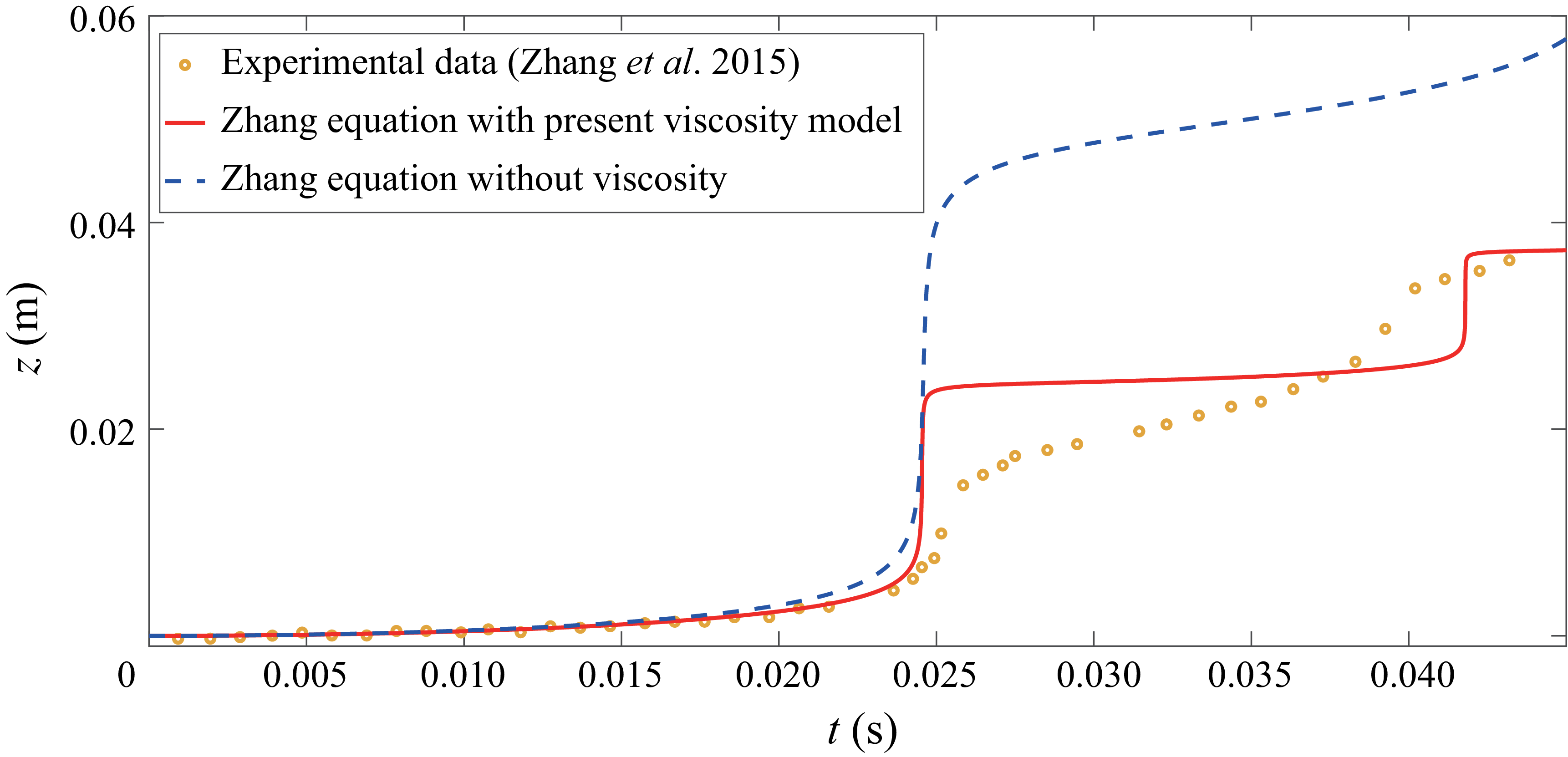

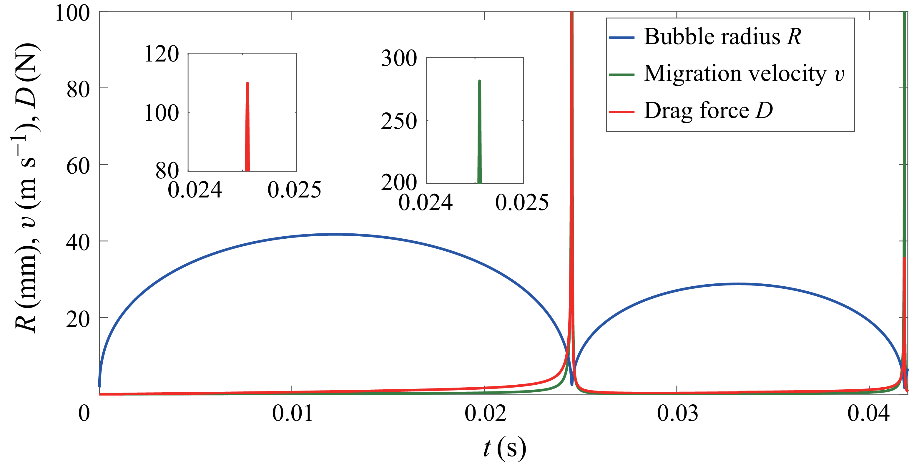


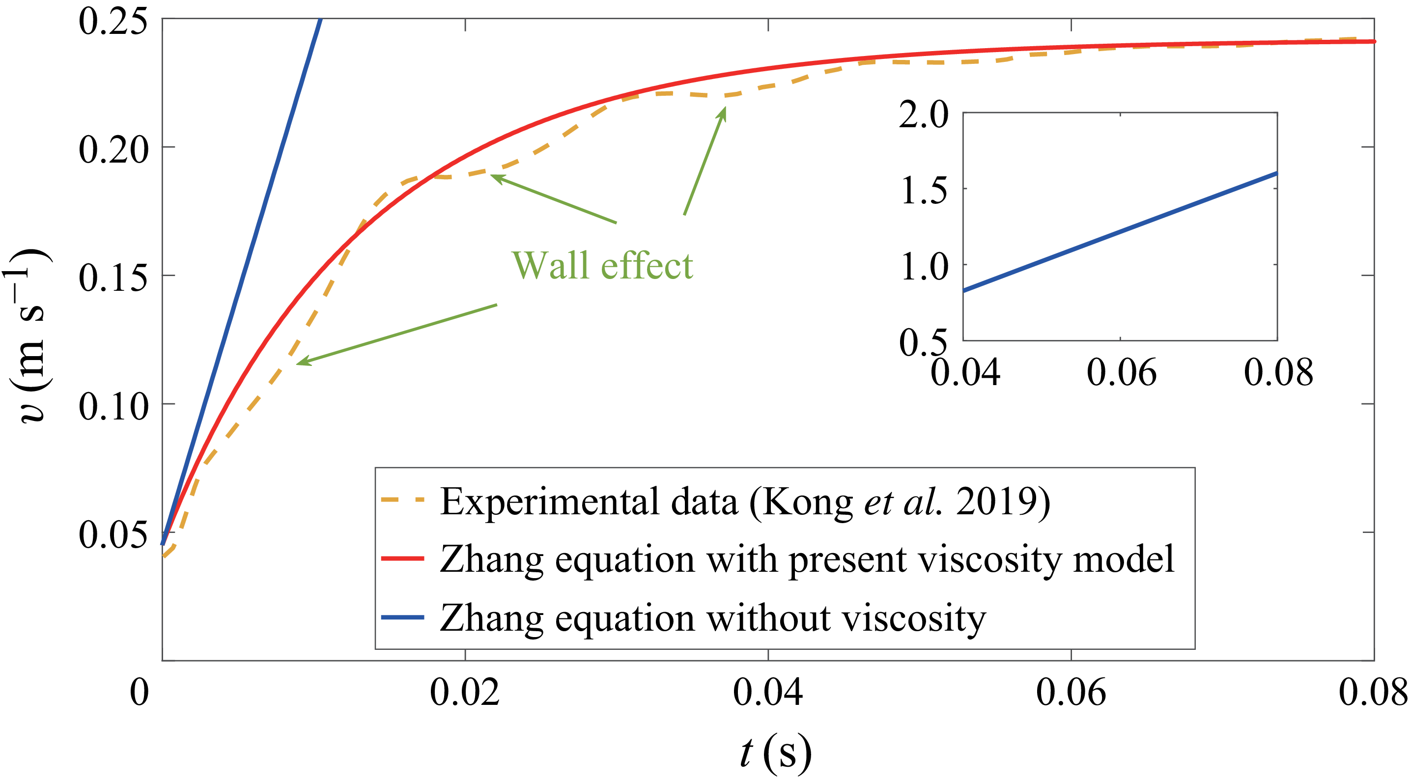

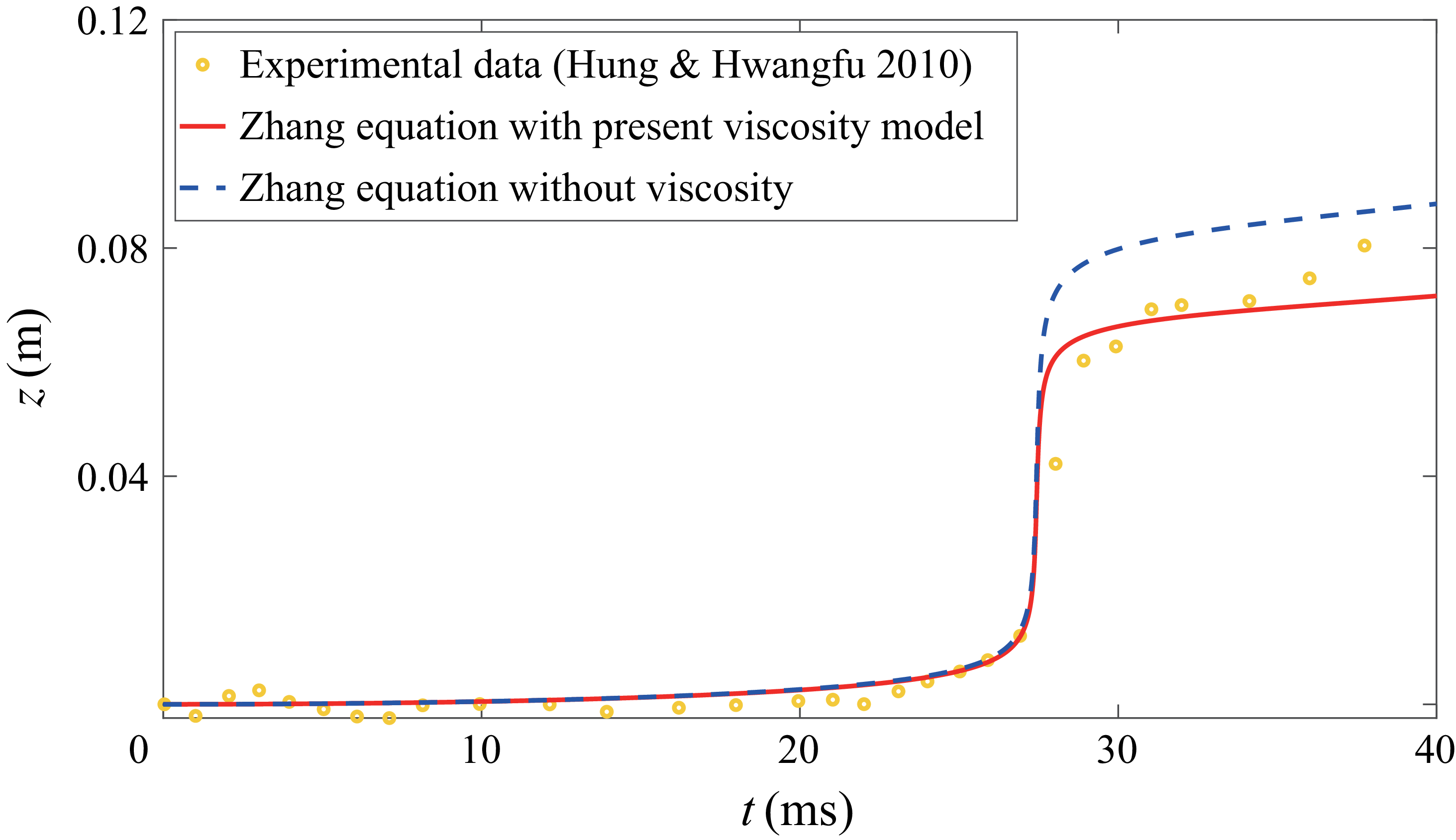

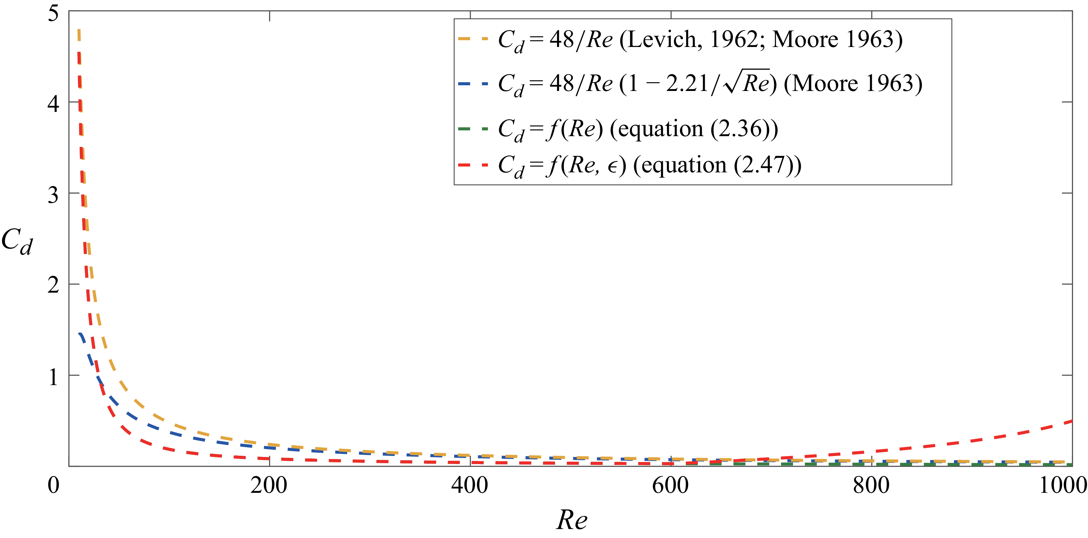


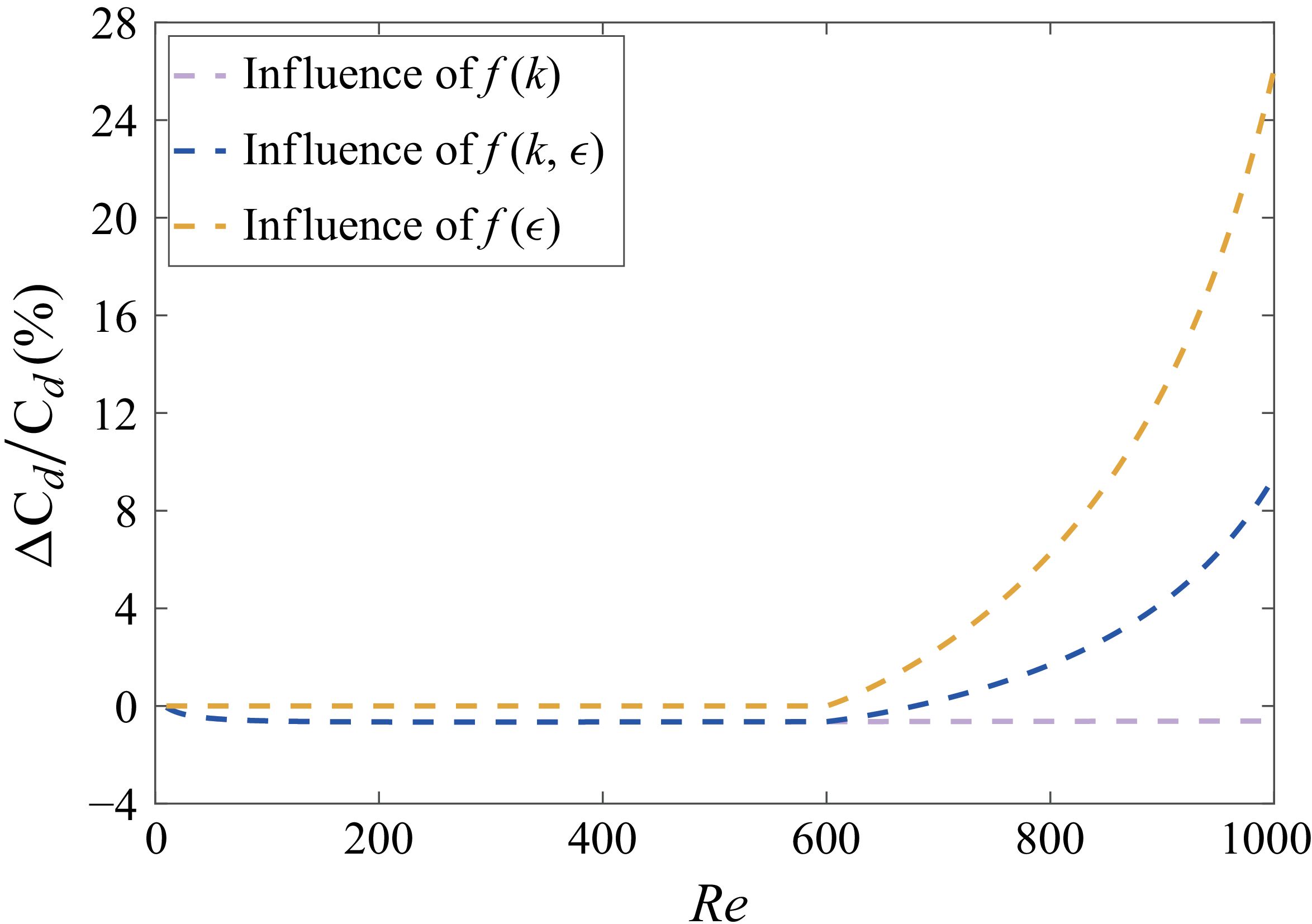


 Open access