


1. Introduction
Stratified exchange flows occur whenever two regions containing fluids with different densities are connected by a narrow duct. These flows have many applications in engineering (e.g. building ventilation, ducts and tunnels), as well as geophysics (e.g. between ocean basins through deep-sea conduits, estuaries and straits). For instance, in estuarine environments the intrusion of salty seawater directly affects coastal habitats. The measurement of turbulence and vertical mixing is challenging due to the high turbulent fluxes (Geyer, Scully & Ralston Reference Geyer, Scully and Ralston2008) and spatiotemporal variability of the inflows and outflows (Burchard et al. Reference Burchard, Lange, Klingbeil and MacCready2019). Such variability in the exchange flow is partially controlled by the channel morphology, which ties turbulent mixing to internal hydraulics. For instance, Chant & Wilson (Reference Chant and Wilson2000) showed that velocity and density have significant along-channel variability in the Hudson River estuary. Similarly, mixing in straits, for example, in the Straits of Gibraltar and Bab el Mandab, is often controlled by internal hydraulic processes (Farmer & Armi Reference Farmer and Armi1988; Pratt et al. Reference Pratt, Johns, Murray and Katsumata1999).
The internal hydraulics of exchange flows have mostly been studied using two-layer models (Armi Reference Armi1986; Lawrence Reference Lawrence1990; Dalziel Reference Dalziel1991). However, when there is significant mixing between the layers, a third, middle layer of intermediate density is formed. Such a three-layer flow was studied in the Strait of Gibraltar by Bray, Ochoa & Kinder (Reference Bray, Ochoa and Kinder1995), who showed with hydrographic observations that the interface was not a sharp boundary but a thick, stratified interfacial layer carrying a substantial portion of the total momentum. The study highlighted the significance of this middle layer due to its shear and demonstrated that two-layer hydraulic models are inadequate for predicting momentum fluxes. Similar three-layer configurations have also been observed in the Strait of Bab al Mandab (Smeed Reference Smeed2000) and the Dardanelles Strait connecting the Aegean Sea to the Sea of Marmara (Jarosz et al. Reference Jarosz, Teague, Book and Beşiktepe2012). In these situations, two-layer hydraulic models do not accurately predict hydraulic controls (i.e. state of maximal exchange flow rate), and more complex multi-layer models are needed (Sannino, Carillo & Artale Reference Sannino, Carillo and Artale2007). The hydraulic control of multi-layer flows was first discussed by Benton (Reference Benton1954) from an energy perspective. Baines (Reference Baines1988) discussed the effects of upstream changes in the hydraulic properties of stratified multi-layer flow over an obstacle and showed that depending on the obstacle height, a hydraulic jump or time-dependent rarefaction might occur. Lane-Serff, Smeed & Postlethwaite (Reference Lane-Serff, Smeed and Postlethwaite2000) used the ‘hydraulic functional’ (Gill Reference Gill1977; Dalziel Reference Dalziel1991) to study multi-layer exchange flows and showed good agreement between a three-layer model and a lock-exchange experiment.
Despite these studies, significant questions remain unresolved in three-layer flows. For example, Pratt et al. (Reference Pratt, Johns, Murray and Katsumata1999) assessed three-layer properties of flow in Bab el Mandab based on acoustic Doppler current profiler velocity measurements. They identified subcritical or supercritical hydraulic flow regimes based on interfacial wave pairs propagating in the same or opposite directions with respect to a given mode. However, the mechanism behind the propagation of these interfacial waves and the local mixing rate is not yet adequately understood.
(a) Schematics of the SID flow configuration. The duct connecting two reservoirs (with different densities) has aspect ratios length-to-height
 $A=L_x^d/L_z^d=30$
and width-to-height
$A=L_x^d/L_z^d=30$
and width-to-height
 $B=L_y^d/L_z^d=1$
. (b) Schematics of the three-layer model. (c–e) Instantaneous snapshots of density fluctuation
$B=L_y^d/L_z^d=1$
. (b) Schematics of the three-layer model. (c–e) Instantaneous snapshots of density fluctuation
 $\rho$
around the reference value: (c) stationary wave (SW), (d) travelling wave (TW) and (e) intermittent turbulence (I).
$\rho$
around the reference value: (c) stationary wave (SW), (d) travelling wave (TW) and (e) intermittent turbulence (I).
The fundamental difference between two- and three-layer internal hydraulics of stratified exchange flows is the possibility of strong interactions between interfacial waves in the presence of the two interfaces separating the three layers. In idealised stratified shear flow and infinitely long domains, the resonant interactions of short-wave instabilities have been studied extensively and understood (Smyth & Carpenter Reference Smyth and Carpenter2019). However, none of the previous studies have explored the possibility of long-wave resonant interactions between interfaces and their potential impact on the evolution of the flow and the triggering of instabilities. Moreover, in realistic conditions, the domain length prescribes finite wavelengths for the longest waves. The resonant interaction between long and short waves has been much less discussed in the literature. Eckart (Reference Eckart1961) and Ma (Reference Ma1981) discussed these long–short-wave interactions theoretically for idealised two-dimensional stratified flows and postulated them to occur when the group velocity of the short waves matches the phase speed of the long waves. However, evidence of such an interaction among long (and short) waves in a realistic situation requires prior knowledge of the variation of the flow on the scales comparable to the wavelength of the long waves, which is typically unavailable in these idealised cases.
The stratified inclined duct (SID) experiment (Meyer & Linden Reference Meyer and Linden2014) has been designed and employed to study stratified exchange flows in laboratory settings that resemble those in nature. In the SID experiment a long duct, which can be tilted at a small angle to the horizontal, connects two reservoirs filled with liquids with different densities (see figure 1). Flows in SID have been studied primarily in laboratory experiments (Lefauve & Linden Reference Lefauve and Linden2020) and more recently by direct numerical simulations (DNS) (Zhu et al. Reference Zhu, Atoufi, Lefauve, Taylor, Kerswell, Dalziel, Lawrence and Linden2023), where excellent agreement has been found.
The DNS of Zhu et al. (Reference Zhu, Atoufi, Lefauve, Taylor, Kerswell, Dalziel, Lawrence and Linden2023) were also analysed using two-layer hydraulics in Atoufi et al. (Reference Atoufi, Zhu, Lefauve, Taylor, Kerswell, Dalziel, Lawrence and Linden2023). The two-layer model is applicable when there is little mixing between the layers, and explains the onset of instability and turbulence. At high turbulence levels, however, the two-layer theory is unable to explain the features observed. Our first main objective in this paper is to analyse the three-layer internal hydraulics of exchange flows including both mixing and viscous effects. Our second main objective is to establish a link between the internal hydraulics and interfacial wave instabilities in three-layer flows by elucidating long–long and long–short-wave resonant interactions.
To achieve these aims, we start by describing our methodology in § 2, extending the SID flow DNS-data-driven approach of Atoufi et al. (Reference Atoufi, Zhu, Lefauve, Taylor, Kerswell, Dalziel, Lawrence and Linden2023) by diagnosing internal hydraulics in three-layer flows with improvements that include both mixing and viscous effects. The three-layer equations and hydraulic regimes are then discussed in § 3, including hydraulic controls as well as control mechanisms. Using this approach, we provide theoretical grounds to link three-layer hydraulics and instabilities in § 4. This allows us to quantify resonant interactions among long waves and between long and short waves, establishing a link with turbulence generation. Finally, we conclude in § 5.
2. Methodology: three-layer reduction of DNS data
2.1. DNS equations and data sets
The schematic of the SID flow is shown in figure 1(a). The configuration consists of a duct with internal height
 $L_z^d$
, width
$L_z^d$
, width
 $L_y^d$
and length
$L_y^d$
and length
 $L_x^d$
connecting two reservoirs filled with fluids at densities
$L_x^d$
connecting two reservoirs filled with fluids at densities
 $\rho _0\pm \Delta \rho /2$
. The entire configuration is inclined at an angle
$\rho _0\pm \Delta \rho /2$
. The entire configuration is inclined at an angle
 $\theta$
to the horizontal. The duct has a square cross-section and is
$\theta$
to the horizontal. The duct has a square cross-section and is
 $30$
times longer than its height, with aspect ratios
$30$
times longer than its height, with aspect ratios
 $A=L_x^d/L_z^d=30$
and
$A=L_x^d/L_z^d=30$
and
 $B=L_y^d/L_z^d=1$
for all cases in this study. Following Lefauve & Linden (Reference Lefauve and Linden2020), Zhu et al. (Reference Zhu, Atoufi, Lefauve, Taylor, Kerswell, Dalziel, Lawrence and Linden2023), we use duct half-height
$B=L_y^d/L_z^d=1$
for all cases in this study. Following Lefauve & Linden (Reference Lefauve and Linden2020), Zhu et al. (Reference Zhu, Atoufi, Lefauve, Taylor, Kerswell, Dalziel, Lawrence and Linden2023), we use duct half-height
 $L_z^d/2$
, half-density difference
$L_z^d/2$
, half-density difference
 $\Delta \rho /2$
for the non-dimensionalisation of lengths and density variations. The velocity is non-dimensionalised based on the averaged velocity difference of two oppositely propagating gravity currents
$\Delta \rho /2$
for the non-dimensionalisation of lengths and density variations. The velocity is non-dimensionalised based on the averaged velocity difference of two oppositely propagating gravity currents
 $\Delta U/2 \equiv \sqrt {g' L_z^d}$
, where
$\Delta U/2 \equiv \sqrt {g' L_z^d}$
, where
 $g'=g\Delta \rho /\rho _0$
is the reduced gravity. We note that this velocity difference across the density interface corresponds to the critical two-layer exchange flow with stability Froude number of unity
$g'=g\Delta \rho /\rho _0$
is the reduced gravity. We note that this velocity difference across the density interface corresponds to the critical two-layer exchange flow with stability Froude number of unity
 $F_\varDelta ^2=(\Delta U/2)^2/ (g' L_z^d )=1$
(Armi Reference Armi1986; Dalziel Reference Dalziel1991; Lawrence Reference Lawrence1993; Atoufi et al. Reference Atoufi, Zhu, Lefauve, Taylor, Kerswell, Dalziel, Lawrence and Linden2023). The non-dimensional parameters then become the tilt angle
$F_\varDelta ^2=(\Delta U/2)^2/ (g' L_z^d )=1$
(Armi Reference Armi1986; Dalziel Reference Dalziel1991; Lawrence Reference Lawrence1993; Atoufi et al. Reference Atoufi, Zhu, Lefauve, Taylor, Kerswell, Dalziel, Lawrence and Linden2023). The non-dimensional parameters then become the tilt angle
 $\theta$
, Reynolds number (
$\theta$
, Reynolds number (
 $\textit{Re} = L_z^d \Delta U /4\nu$
) and Prandtl number (
$\textit{Re} = L_z^d \Delta U /4\nu$
) and Prandtl number (
 $Pr =\nu /\kappa$
), where
$Pr =\nu /\kappa$
), where
 $\nu$
and
$\nu$
and
 $\kappa$
are momentum and mass diffusivity, respectively. The bulk Richardson number is, by definition,
$\kappa$
are momentum and mass diffusivity, respectively. The bulk Richardson number is, by definition,
 \begin{eqnarray} {Ri}=\dfrac {g \frac {\Delta \rho }{2} \frac {L_z^d}{2}}{\rho _0 \left (\frac {\Delta U}{2} \right )^2}=\frac {1}{4}, \end{eqnarray}
a constant in all cases in this study. The governing equations for the velocity field
 $\boldsymbol{u}$
and density fluctuations
$\boldsymbol{u}$
and density fluctuations
 $\rho$
around the reference value are the forced Navier–Stokes equations under the Boussinesq approximation that takes the dimensionless form
$\rho$
around the reference value are the forced Navier–Stokes equations under the Boussinesq approximation that takes the dimensionless form
 \begin{align} \boldsymbol{\nabla } \cdot \boldsymbol{u} &= 0, \end{align}
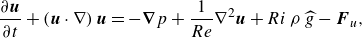 \begin{align} \frac {\partial \boldsymbol{u}}{\partial t} + \left (\boldsymbol{u} \cdot \nabla \right ) \boldsymbol{u} &= - \boldsymbol{\nabla }p + \frac {1}{{Re}} \nabla ^{2}\boldsymbol{u} + {Ri}\, \rho \, \widehat { g } - \boldsymbol{F}_u, \end{align}
 \begin{align} \frac {\partial \rho }{\partial t} + \left (\boldsymbol{u} \cdot \nabla \right ) \rho &= \frac {1}{{Re\;Pr}} \nabla ^{2}\rho - F_\rho, \end{align}
where
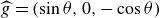 $\widehat {g}=(\sin {\theta },0,-\cos {\theta })$
is the direction of gravity in the duct coordinate system (figure 1). The flow is driven in the streamwise
$\widehat {g}=(\sin {\theta },0,-\cos {\theta })$
is the direction of gravity in the duct coordinate system (figure 1). The flow is driven in the streamwise
 $\widehat {x}$
direction and confined by solid walls in the spanwise direction
$\widehat {x}$
direction and confined by solid walls in the spanwise direction
 $\widehat {y}$
. The
$\widehat {y}$
. The
 $\boldsymbol{F}_u$
and
$\boldsymbol{F}_u$
and
 $F_\rho$
are forcing terms used to maintain the quasi-steady exchange flow, as described in Zhu et al. (Reference Zhu, Atoufi, Lefauve, Taylor, Kerswell, Dalziel, Lawrence and Linden2023). They are ONLY applied in a narrow region inside the reservoirs to sustain the flow without using excessively large reservoirs.
$F_\rho$
are forcing terms used to maintain the quasi-steady exchange flow, as described in Zhu et al. (Reference Zhu, Atoufi, Lefauve, Taylor, Kerswell, Dalziel, Lawrence and Linden2023). They are ONLY applied in a narrow region inside the reservoirs to sustain the flow without using excessively large reservoirs.
The governing equations are solved numerically using a compact sixth-order finite difference scheme for spatial derivatives and a third-order Adam-Bashforth scheme for time integration using the open-source solver Xcompact3D (Bartholomew et al. Reference Bartholomew, Deskos, Frantz, Schuch, Lamballais and Laizet2020) modified to include
 $F_\rho$
and
$F_\rho$
and
 $\boldsymbol{F}_u$
. For the full details of the numerical approach and comparison with experiments, the reader is referred to Zhu et al. (Reference Zhu, Atoufi, Lefauve, Taylor, Kerswell, Dalziel, Lawrence and Linden2023).
$\boldsymbol{F}_u$
. For the full details of the numerical approach and comparison with experiments, the reader is referred to Zhu et al. (Reference Zhu, Atoufi, Lefauve, Taylor, Kerswell, Dalziel, Lawrence and Linden2023).
In this study we consider the laminar (L), stationary wave (SW), travelling wave (TW) and intermittent (I) datasets that correspond to
 $\theta =2^\circ , 5^\circ , 6^\circ\,\text{and} \, 7^\circ$
, respectively. All these cases are at the moderate Reynolds number
$\theta =2^\circ , 5^\circ , 6^\circ\,\text{and} \, 7^\circ$
, respectively. All these cases are at the moderate Reynolds number
 ${Re}=650$
and Prandtl number
${Re}=650$
and Prandtl number
 ${Pr}=7$
, representing thermal stratification in water. For detailed flow visualisations of the velocity and density fields corresponding to these regimes, readers are referred to Zhu et al. (Reference Zhu, Atoufi, Lefauve, Taylor, Kerswell, Dalziel, Lawrence and Linden2023), specifically their figure 5 and the supplementary materials, which include simulation movies.
${Pr}=7$
, representing thermal stratification in water. For detailed flow visualisations of the velocity and density fields corresponding to these regimes, readers are referred to Zhu et al. (Reference Zhu, Atoufi, Lefauve, Taylor, Kerswell, Dalziel, Lawrence and Linden2023), specifically their figure 5 and the supplementary materials, which include simulation movies.
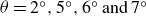
Layer splitting based on nearest turning points, illustrated by (a) mean density profiles, (b) gradient Richardson number
 ${Ri}_g$
as defined in (2.8) and (c) the second derivative of the mean density profile,
${Ri}_g$
as defined in (2.8) and (c) the second derivative of the mean density profile,
 $\partial ^2 \langle \rho \rangle / \partial z^2$
. Markers indicate the nearest turning points to the mid-isopycnals where
$\partial ^2 \langle \rho \rangle / \partial z^2$
. Markers indicate the nearest turning points to the mid-isopycnals where
 $\langle \rho \rangle = 0$
in each case.
$\langle \rho \rangle = 0$
in each case.
2.2. Three-layer averaging
We reduce the dimensionality of the DNS data and cluster it into three distinct layers as sketched in figure 1(b). These distinct layers consist of a middle mixed layer between two other layers one above and another below as can be seen from the density snapshots in figure 1(c,d) for the TW and I cases. The three-layer structure of the density field for non-laminar cases is clear from the mean density profiles shown in figure 2(a). The slopes of the density profiles change in
 $-0.3 \leqslant z \leqslant 0.3$
for the SW, TW and I cases and, as a result of mixing, become closer to vertical than the L case in which the density profile can be reasonably considered as a two-layer profile.
$-0.3 \leqslant z \leqslant 0.3$
for the SW, TW and I cases and, as a result of mixing, become closer to vertical than the L case in which the density profile can be reasonably considered as a two-layer profile.
We first average the velocity and density from simulation data over the
 $y$
direction (denoted by
$y$
direction (denoted by
 $\langle \bullet \rangle _y = (1/2)\int _{-1}^{1} \bullet \,{\rm d}y$
). We then locate the lower and upper interfaces from
$\langle \bullet \rangle _y = (1/2)\int _{-1}^{1} \bullet \,{\rm d}y$
). We then locate the lower and upper interfaces from
 $\langle \rho \rangle _y$
that are denoted by
$\langle \rho \rangle _y$
that are denoted by
 $\eta _2(x,t)$
and
$\eta _2(x,t)$
and
 $\eta _1(x,t)$
, respectively (figure 1
b).
$\eta _1(x,t)$
, respectively (figure 1
b).
To identify the bottom and top interfaces, we first locate the mid-isopycnal where
 $\langle \rho \rangle _y =0$
, as the dimensionless spanwise average density is
$\langle \rho \rangle _y =0$
, as the dimensionless spanwise average density is
 $-1 \leqslant \langle \rho \rangle _y \leqslant 1$
. The elevation of the mid-isopycnal is denoted by
$-1 \leqslant \langle \rho \rangle _y \leqslant 1$
. The elevation of the mid-isopycnal is denoted by
 $\eta _0(x,t)$
. The location of the bottom and top interfaces are marked using the inner turning points of
$\eta _0(x,t)$
. The location of the bottom and top interfaces are marked using the inner turning points of
 $\langle \rho \rangle _y$
, i.e. the points nearest to the mid-isopycnal where
$\langle \rho \rangle _y$
, i.e. the points nearest to the mid-isopycnal where
 $\partial ^2 \langle \rho \rangle _y/ \partial z^2 = 0$
(figure 2). Those turning points with height
$\partial ^2 \langle \rho \rangle _y/ \partial z^2 = 0$
(figure 2). Those turning points with height
 $z=\eta _2(x,t) \lt \eta _0$
mark the location of the lower interface and those with height
$z=\eta _2(x,t) \lt \eta _0$
mark the location of the lower interface and those with height
 $z=\eta _1(x,t) \gt \eta _0$
mark the location of the upper interface.
$z=\eta _1(x,t) \gt \eta _0$
mark the location of the upper interface.
We compute the layer-averaged velocities
 $u_i$
, heights
$u_i$
, heights
 $h_i$
and densities
$h_i$
and densities
 $\rho _i$
(where
$\rho _i$
(where
 $i=0,1,2$
correspond to the middle, upper and lower layer, respectively) as height averages
$i=0,1,2$
correspond to the middle, upper and lower layer, respectively) as height averages
 \begin{align} h_1(x,t)=1-\eta _1(x,t), \quad u_1(x,t)=\langle \langle u\rangle _y\rangle _{z_1}, \quad \rho _1(x,t)=\langle \langle \rho \rangle _y\rangle _{z_1},\end{align}
 \begin{align} h_0(x,t)=\eta _1(x,t)-\eta _2(x,t), \quad u_0(x,t)=\langle \langle u\rangle _y\rangle _{z_0}, \quad \rho _0(x,t)=\langle \langle \rho \rangle _y\rangle _{z_0},\end{align}
 \begin{align} h_2(x,t)=1+\eta _2(x,t), \quad u_2(x,t)=\langle \langle u\rangle _y\rangle _{z_2}, \quad \rho _2(x,t)=\langle \langle \rho \rangle _y\rangle _{z_2},\end{align}
where the top layer average is
 $\langle \bullet \rangle _{z_1} =(1/h_1)\int _{\eta _1}^{1}\bullet \ {\rm d}z$
, the middle layer average is given by
$\langle \bullet \rangle _{z_1} =(1/h_1)\int _{\eta _1}^{1}\bullet \ {\rm d}z$
, the middle layer average is given by
 $ \langle \bullet \rangle _{z_0} = (1/h_0)\int _{\eta _2}^{\eta _1}\bullet \ {\rm d}z$
and the bottom layer average is
$ \langle \bullet \rangle _{z_0} = (1/h_0)\int _{\eta _2}^{\eta _1}\bullet \ {\rm d}z$
and the bottom layer average is
 $ \langle \bullet \rangle _{z_2} = (1/h_2)\int _{-1}^{\eta _2}\bullet \ {\rm d}z$
. We note that
$ \langle \bullet \rangle _{z_2} = (1/h_2)\int _{-1}^{\eta _2}\bullet \ {\rm d}z$
. We note that
 $z=1$
and
$z=1$
and
 $z=-1$
are the non-dimensional height of the top and bottom walls, respectively.
$z=-1$
are the non-dimensional height of the top and bottom walls, respectively.
As shown in figure 2(b), the gradient Richardson number defined based on velocity and density fields averaged over the duct length, cross-sections and time, i.e.
 \begin{equation} {Ri}_g\equiv -{Ri}\,\frac {{\partial _z \langle \rho \rangle }_{x,y,t}}{{(\partial _z \langle u \rangle _{x,y,t}})^2}, \end{equation}
is reasonably constant in the middle layer
 $\eta _1 \lt z \lt \eta _2$
and approximately equal to
$\eta _1 \lt z \lt \eta _2$
and approximately equal to
 $0.5$
for the laminar case and
$0.5$
for the laminar case and
 $0.15$
for other cases. These values are consistent with the critical values for the local Richardson number observed in previous experimental studies (Lefauve & Linden Reference Lefauve and Linden2020; Jiang et al. Reference Jiang, Lefauve, Dalziel and Linden2022, Reference Jiang, Atoufi, Zhu, Lefauve, Taylor, Dalziel and Linden2023).
$0.15$
for other cases. These values are consistent with the critical values for the local Richardson number observed in previous experimental studies (Lefauve & Linden Reference Lefauve and Linden2020; Jiang et al. Reference Jiang, Lefauve, Dalziel and Linden2022, Reference Jiang, Atoufi, Zhu, Lefauve, Taylor, Dalziel and Linden2023).
2.3. Evolution of layer-averaged quantities
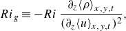
The velocity and heights of the three layers for the TW case are shown in figure 3 in
 $x{-}t$
(space–time) plots. We observe sudden changes in the layer thicknesses in the central region of the duct, indicated by the sharp transitions in contour colours, which we consider to be the locations of internal hydraulic jumps. The trajectories of these jumps are marked with two curves (dashed and dashed-dotted, corresponding to the upper and lower interfaces, respectively). We observe the region between these lines progressively extends towards both ends of the duct at later times. Consistent with the variations in layer heights, the layer velocities (
$x{-}t$
(space–time) plots. We observe sudden changes in the layer thicknesses in the central region of the duct, indicated by the sharp transitions in contour colours, which we consider to be the locations of internal hydraulic jumps. The trajectories of these jumps are marked with two curves (dashed and dashed-dotted, corresponding to the upper and lower interfaces, respectively). We observe the region between these lines progressively extends towards both ends of the duct at later times. Consistent with the variations in layer heights, the layer velocities (
 $u_0, u_1, u_2$
) also change abruptly at the same locations (see figure 3
e–f). Note that the middle layer
$u_0, u_1, u_2$
) also change abruptly at the same locations (see figure 3
e–f). Note that the middle layer
 $h_0$
, which is initially located near the duct centre (
$h_0$
, which is initially located near the duct centre (
 $x \approx 0$
) at
$x \approx 0$
) at
 $t = 80$
due to internal hydraulic jumps on the upper and lower interfaces, grows as the jumps propagate and eventually spread to occupy almost the entire duct by
$t = 80$
due to internal hydraulic jumps on the upper and lower interfaces, grows as the jumps propagate and eventually spread to occupy almost the entire duct by
 $t \approx 200$
.
$t \approx 200$
.
Space–time (
 $x$
–
$x$
–
 $t$
) plots of layer heights and velocities obtained from DNS for the TW case, assuming a three-layer model: (a,b,c) represent the heights and (d,e,f) the velocities of the upper, middle and lower layers, respectively. Dashed and dash-dotted lines indicate abrupt changes in the heights of the upper and lower edges of the middle layer, respectively, corresponding to identical changes in velocities across all panels.
$t$
) plots of layer heights and velocities obtained from DNS for the TW case, assuming a three-layer model: (a,b,c) represent the heights and (d,e,f) the velocities of the upper, middle and lower layers, respectively. Dashed and dash-dotted lines indicate abrupt changes in the heights of the upper and lower edges of the middle layer, respectively, corresponding to identical changes in velocities across all panels.
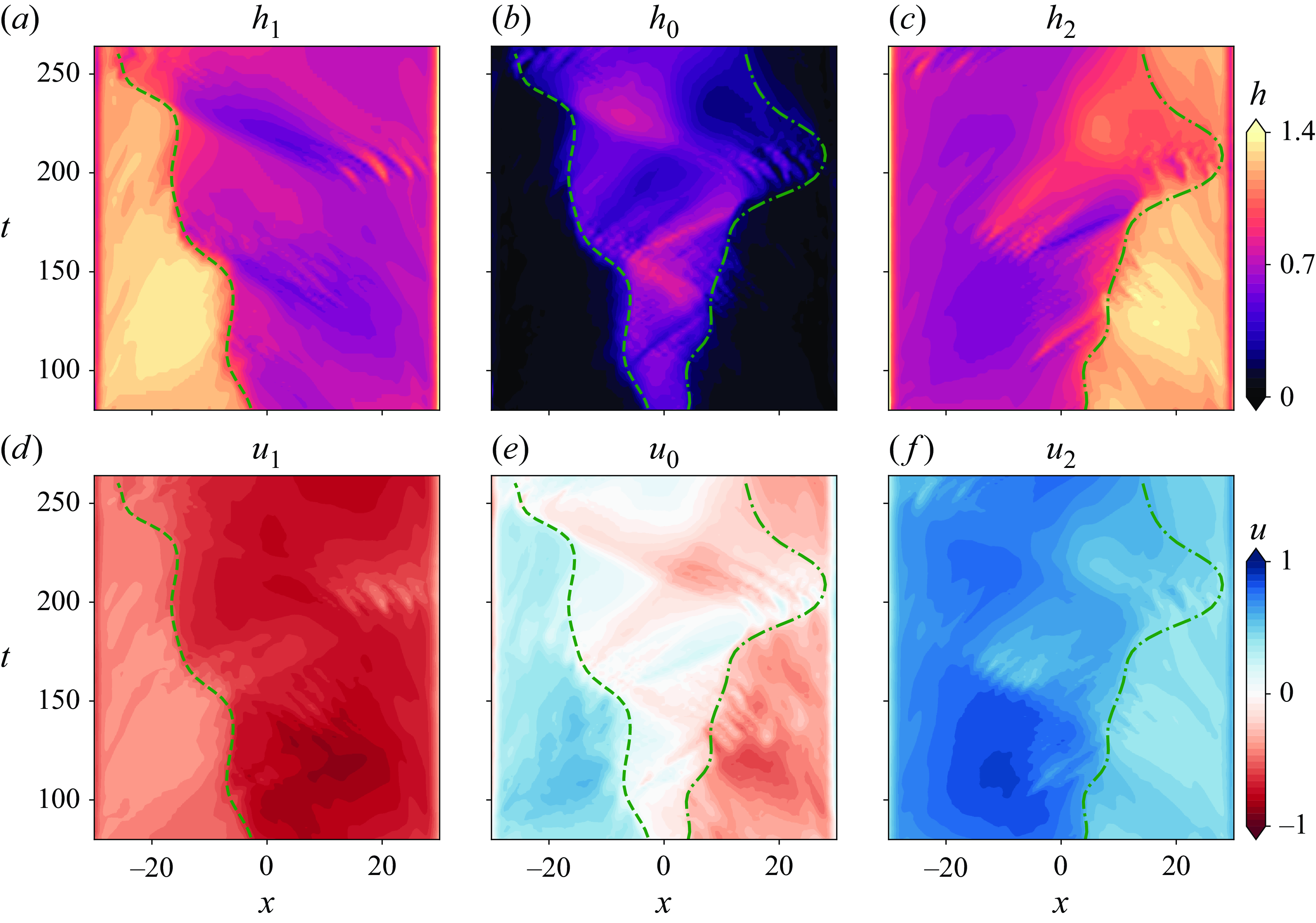
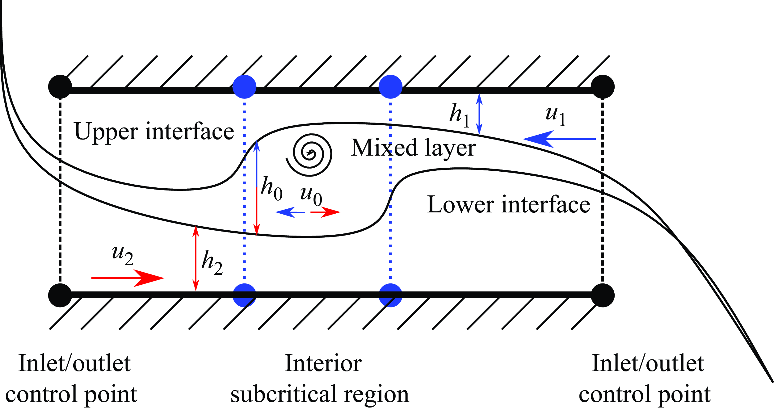
Figure 4 shows a schematic of the three-layer hydraulic jumps observed in the TW case. Near the left of the dashed line in figure 3(a,b),
 $h_0$
increases with a corresponding decrease in the upper layer thickness
$h_0$
increases with a corresponding decrease in the upper layer thickness
 $h_1$
. The middle layer velocity
$h_1$
. The middle layer velocity
 $u_0$
is generally positive on the left side of the dashed line (associated with the location of the upper interface) but reduces to almost zero on the right side of the dashed line. Near the hydraulic jump, the velocities of the upper and middle layers have opposite signs (figure 3
d,e) associated with a large difference in their respective heights (figure 3
a,b). Such strong shear and asymmetry trigger instabilities and the upper interface becomes unstable. The bottom and middle layers have the same flow direction on the left side of the dashed line (figure 3
d,f) and, therefore, have smaller shear; thus the lower interface is more stable here. A similar explanation can be provided for the instability of the lower interface by comparing the velocity and height differences between the middle and lower layers at the neighbourhood of the right hydraulic jump (dashed-dotted lines) as illustrated in figure 4. These jumps in the layer heights and velocities and the associated turbulence generation are further linked to three-layer internal hydraulics in the next section.
$u_0$
is generally positive on the left side of the dashed line (associated with the location of the upper interface) but reduces to almost zero on the right side of the dashed line. Near the hydraulic jump, the velocities of the upper and middle layers have opposite signs (figure 3
d,e) associated with a large difference in their respective heights (figure 3
a,b). Such strong shear and asymmetry trigger instabilities and the upper interface becomes unstable. The bottom and middle layers have the same flow direction on the left side of the dashed line (figure 3
d,f) and, therefore, have smaller shear; thus the lower interface is more stable here. A similar explanation can be provided for the instability of the lower interface by comparing the velocity and height differences between the middle and lower layers at the neighbourhood of the right hydraulic jump (dashed-dotted lines) as illustrated in figure 4. These jumps in the layer heights and velocities and the associated turbulence generation are further linked to three-layer internal hydraulics in the next section.
A schematic of the internal hydraulic jumps in SID flows.
3. Three-layer hydraulics: characteristics, regimes and control mechanisms
In the previous section we discussed temporal and along-duct variations of layer heights and velocities (mainly for the SW and TW cases) and postulated a possible link between such variation in layer properties and instability and the transition to turbulence. In this section we introduce viscous, non-hydrostatic three-layer equations that describe the internal hydraulics of stratified turbulent exchange flows in § 3.1. These equations also govern the dynamics of DNS data using the three-layer averaging procedure described in § 2.2. Building upon the characteristics of the three-layer equations, we demonstrate information propagation in § 3.2 and identify three-layer hydraulic control and hydraulic transitions in § 3.3. We then show their strong correlation to turbulence generation in § 3.3.3. In § 3.4 we discuss the regularisation of the three-layer exchange flow near the hydraulic control points (i.e. hydraulic control mechanisms).
3.1. Three-layer evolution equations
To identify mechanisms governing the evolution of three-layer exchange flow, we perform a layer-wise integration of (2.2)–(2.4) as described in § 2.2, noting that
 $\boldsymbol{F}_u=\boldsymbol{0}, F_\rho=0$
inside the duct where DNS data were collected. This procedure leads to the viscous three-layer equations and can be written in the general vector form as
$\boldsymbol{F}_u=\boldsymbol{0}, F_\rho=0$
inside the duct where DNS data were collected. This procedure leads to the viscous three-layer equations and can be written in the general vector form as
 \begin{equation} \unicode{x1D63E}\frac {\partial \boldsymbol{q}}{\partial t}+\unicode{x1D63C}\frac {\partial \boldsymbol{q}}{\partial x}=\unicode{x1D63D}\frac {\partial \boldsymbol{s}}{\partial x}+{\boldsymbol{\tau }} \boldsymbol{q}+\boldsymbol{\mathcal{F}}, \end{equation}
where the state vector is defined as
 $\boldsymbol{q}=[u_1,u_0,u_2,h_1,h_0,h_2]^T$
, recalling that the subscripts identify the velocities and heights of the upper (1), middle (0) and lower (2) layer, respectively, as sketched in figure 1(b). The coefficient matrices on the left-hand side of (3.1) are
$\boldsymbol{q}=[u_1,u_0,u_2,h_1,h_0,h_2]^T$
, recalling that the subscripts identify the velocities and heights of the upper (1), middle (0) and lower (2) layer, respectively, as sketched in figure 1(b). The coefficient matrices on the left-hand side of (3.1) are
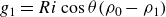
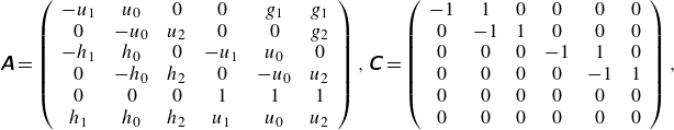 \begin{eqnarray} \unicode{x1D63C}= \left (\begin{array}{cccccc} -u_1 & u_0 & 0 & 0 & g_1 & g_1\\ 0 & -u_0 & u_2 & 0 & 0 & g_2 \\ -h_1 & h_0 & 0 & -u_1 & u_0 & 0\\ 0 & -h_0 & h_2 & 0 & -u_0 & u_2 \\ 0 & 0 & 0 & 1 & 1 & 1\\ h_1 & h_0 & h_2 & u_1 & u_0 & u_2 \end{array}\right ) , \unicode{x1D63E}= \left (\begin{array}{cccccc} -1 & 1 & 0 & 0 & 0 & 0\\ 0 & -1 & 1 & 0 & 0 & 0 \\ 0 & 0 & 0 & -1 & 1 & 0\\ 0 & 0 & 0 & 0 & -1 & 1 \\ 0 & 0 & 0 & 0 & 0 & 0\\ 0 & 0 & 0 & 0 & 0 & 0 \end{array}\right ),\nonumber \\ && \end{eqnarray}
where
 $g_1={Ri} \cos {\theta } (\rho _0-\rho _1 )$
and
$g_1={Ri} \cos {\theta } (\rho _0-\rho _1 )$
and
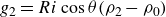 $g_2={Ri} \cos {\theta } (\rho _2-\rho _0 )$
are the dimensionless reduced gravity at the upper and lower interfaces, respectively. The forcing terms,
$g_2={Ri} \cos {\theta } (\rho _2-\rho _0 )$
are the dimensionless reduced gravity at the upper and lower interfaces, respectively. The forcing terms,
 $\unicode{x1D63D}\,\partial \boldsymbol{s}/\partial x$
and
$\unicode{x1D63D}\,\partial \boldsymbol{s}/\partial x$
and
 ${\tau } \boldsymbol{q}$
, are due to buoyancy and viscous stresses and are discussed in detail in § 3.4. The gravity tensor reads as
${\tau } \boldsymbol{q}$
, are due to buoyancy and viscous stresses and are discussed in detail in § 3.4. The gravity tensor reads as
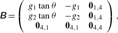 \begin{eqnarray} \unicode{x1D63D}= \left (\begin{array}{cccccc} g_1 \tan {\theta } & -g_1 & \boldsymbol{0}_{1,4}\\ g_2 \tan {\theta } & -g_2 & \boldsymbol{0}_{1,4} \\ \boldsymbol{0}_{4,1} & \boldsymbol{0}_{4,1} & \boldsymbol{0}_{4,4} \end{array}\right ), \end{eqnarray}
where
 $\boldsymbol{0}_{m,n}$
denotes the block null matrix of the size
$\boldsymbol{0}_{m,n}$
denotes the block null matrix of the size
 $m \times n$
and
$m \times n$
and
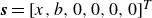 $\boldsymbol{s}=[x,b,0,0,0,0]^T$
is the vector associated with geometry change. Here
$\boldsymbol{s}=[x,b,0,0,0,0]^T$
is the vector associated with geometry change. Here
 $b(x)$
denotes the elevation of the bottom wall where
$b(x)$
denotes the elevation of the bottom wall where
 $b(x)=-1$
throughout the duct but abruptly changes to
$b(x)=-1$
throughout the duct but abruptly changes to
 $b(x)=-2$
at the inlet/outlet. The model for the viscous stress tensor for three-layer hydraulics is a sparse
$b(x)=-2$
at the inlet/outlet. The model for the viscous stress tensor for three-layer hydraulics is a sparse
 $6 \times 6$
matrix,
$6 \times 6$
matrix,
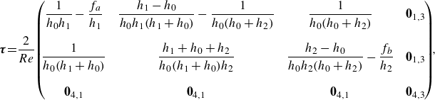 \begin{eqnarray} {\boldsymbol{\tau }}\!=\!\frac {2}{{Re}} \!\left (\!\!\!\!\begin{array}{cccccc} \dfrac {1}{h_0 h_1} -\dfrac {f_a}{h_1} & \dfrac {h_1-h_0}{h_0 h_1 (h_1+h_0)}-\dfrac {1 }{h_0 (h_0+h_2)} & \dfrac {1}{h_0 (h_0+h_2)} & \boldsymbol{0}_{1,3} \\ \\ \dfrac {1}{h_0 (h_1+h_0)} & \dfrac {h_1+h_0+h_2}{h_0 (h_1+h_0)h_2} & \dfrac {h_2-h_0}{h_0 h_2 (h_0+h_2)}-\dfrac {f_b }{ h_2} & \boldsymbol{0}_{1,3} \\ \\ \boldsymbol{0}_{4,1} & \boldsymbol{0}_{4,1} & \boldsymbol{0}_{4,1} & \boldsymbol{0}_{4,3} \end{array}\!\!\!\right )\!\!,\nonumber\\&& \end{eqnarray}
where
 $f_a$
and
$f_a$
and
 $f_b$
are the slip-with-friction coefficients at the upper and lower boundaries. These coefficients are computed based on
$f_b$
are the slip-with-friction coefficients at the upper and lower boundaries. These coefficients are computed based on
 $f \langle u \rangle _y = \partial \langle u \rangle _y/\partial z$
at the bottom and top boundaries from DNS data. For a free-slip condition
$f \langle u \rangle _y = \partial \langle u \rangle _y/\partial z$
at the bottom and top boundaries from DNS data. For a free-slip condition
 $f=0$
and for the no-slip condition,
$f=0$
and for the no-slip condition,
 $f$
is proportional to
$f$
is proportional to
 ${Re}$
. The forcing term
${Re}$
. The forcing term
 $\mathcal{F}=[\mathcal{F}_1, \mathcal{F}_0, \mathcal{F}_2, 0, 0, 0]^T$
is due to the non-hydrostatic pressure gradient and is determined from DNS data (note that this contribution is weaker than the hydrostatic pressure gradient in all cases considered here; see Atoufi et al. Reference Atoufi, Zhu, Lefauve, Taylor, Kerswell, Dalziel, Lawrence and Linden2023). If
$\mathcal{F}=[\mathcal{F}_1, \mathcal{F}_0, \mathcal{F}_2, 0, 0, 0]^T$
is due to the non-hydrostatic pressure gradient and is determined from DNS data (note that this contribution is weaker than the hydrostatic pressure gradient in all cases considered here; see Atoufi et al. Reference Atoufi, Zhu, Lefauve, Taylor, Kerswell, Dalziel, Lawrence and Linden2023). If
 $\boldsymbol{\mathcal{F}}=0$
, (3.1) reduce to the viscous shallow water equations.
$\boldsymbol{\mathcal{F}}=0$
, (3.1) reduce to the viscous shallow water equations.
3.2. Information propagation
We now investigate, using (3.1), the directions in which information is carried by long interfacial waves in a three-layer configuration, dictating the hydraulic regime. Consider a left eigenvector
 $\boldsymbol{v}$
and eigenvalue
$\boldsymbol{v}$
and eigenvalue
 $\lambda$
associated with the coefficient matrix pair
$\lambda$
associated with the coefficient matrix pair
 $(\unicode{x1D63C}$
,
$(\unicode{x1D63C}$
,
 $\unicode{x1D63E}{\kern2pt})$
such that
$\unicode{x1D63E}{\kern2pt})$
such that
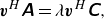 \begin{eqnarray} \boldsymbol{v}^H \unicode{x1D63C} = \lambda \boldsymbol{v}^H \unicode{x1D63E} ,\end{eqnarray}
where the superscript
 $H$
denotes the Hermitian transpose. Multiplying (3.1) by
$H$
denotes the Hermitian transpose. Multiplying (3.1) by
 $\boldsymbol{v}^H$
and rewriting
$\boldsymbol{v}^H$
and rewriting
 ${\boldsymbol{\tau }}= \unicode{x1D63E} \unicode{x1D63F}$
yields
${\boldsymbol{\tau }}= \unicode{x1D63E} \unicode{x1D63F}$
yields
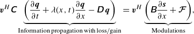 \begin{eqnarray} \boldsymbol{v}^H \unicode{x1D63E} \underbrace {\left (\frac {\partial \boldsymbol{q}}{\partial t}+\lambda (x,t) \frac {\partial \boldsymbol{q}}{\partial x} - \unicode{x1D63F}\kern2pt \boldsymbol{q}\right )}_{\rm{Information\,propagation\,with\,loss/gain}} = \boldsymbol{v}^H \underbrace {\left (\unicode{x1D63D}\frac {\partial \boldsymbol{s}}{\partial x}+\boldsymbol{\mathcal{F}} \right )}_{\rm{Modulations}}, \end{eqnarray}
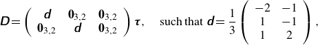
where
 \begin{eqnarray} \unicode{x1D63F}= \left (\begin{array}{cccccc} \unicode{x1D63F} & \boldsymbol{0}_{3,2} & \boldsymbol{0}_{3,2} \\ \boldsymbol{0}_{3,2} & \unicode{x1D63F} & \boldsymbol{0}_{3,2} \end{array}\right ) {\boldsymbol{\tau }}, \quad {\rm such\, that} \ \unicode{x1D63F}=\frac {1}{3} \left (\begin{array}{cccccc} -2 & -1 \\ 1 & -1 \\ 1 & 2 \end{array}\right ) ,\end{eqnarray}
is the diffusion matrix obtained by a singular value decomposition of
 $\unicode{x1D63E}=\unicode{x1D650} \unicode{x1D64C} \unicode{x1D651}^H$
, where
$\unicode{x1D63E}=\unicode{x1D650} \unicode{x1D64C} \unicode{x1D651}^H$
, where
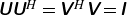 $\unicode{x1D650} \unicode{x1D650}^H=\unicode{x1D651}^H\unicode{x1D651}=\unicode{x1D644}$
and
$\unicode{x1D650} \unicode{x1D650}^H=\unicode{x1D651}^H\unicode{x1D651}=\unicode{x1D644}$
and
 $\unicode{x1D64C}$
is a diagonal matrix leading to
$\unicode{x1D64C}$
is a diagonal matrix leading to
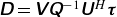 $\unicode{x1D63F}=\unicode{x1D651} \unicode{x1D64C}^{-1} \unicode{x1D650}^H {\boldsymbol{\tau }}$
.
$\unicode{x1D63F}=\unicode{x1D651} \unicode{x1D64C}^{-1} \unicode{x1D650}^H {\boldsymbol{\tau }}$
.
Recall that
 $\unicode{x1D63F}\kern2pt \boldsymbol{q}$
is solely due to viscous effects and when absorbed in the left-hand side of (3.6) it can be viewed as a mechanism affecting the propagation of information contained in
$\unicode{x1D63F}\kern2pt \boldsymbol{q}$
is solely due to viscous effects and when absorbed in the left-hand side of (3.6) it can be viewed as a mechanism affecting the propagation of information contained in
 $\boldsymbol{q}$
.
$\boldsymbol{q}$
.
Equation (3.6) is particularly useful in explaining various mechanisms affecting the propagation of information in stratified turbulent exchange flows. In the limit where viscous stresses are neglected (
 $\unicode{x1D63F}=\boldsymbol{0}$
), non-hydrostatic pressure gradients are ignored (
$\unicode{x1D63F}=\boldsymbol{0}$
), non-hydrostatic pressure gradients are ignored (
 $\boldsymbol{\mathcal{F}}=\boldsymbol{0}$
), in the interior region when the configuration is horizontal (
$\boldsymbol{\mathcal{F}}=\boldsymbol{0}$
), in the interior region when the configuration is horizontal (
 $\unicode{x1D63D}\kern1.5pt{\partial \boldsymbol{s}}/{\partial x}=\boldsymbol{0}$
) then (3.6) will be homogeneous.
$\unicode{x1D63D}\kern1.5pt{\partial \boldsymbol{s}}/{\partial x}=\boldsymbol{0}$
) then (3.6) will be homogeneous.
In the homogeneous limit, the coordinate transformation
 $2 \xi =t+x/\lambda$
(
$2 \xi =t+x/\lambda$
(
 $\lambda \ne 0$
) yields
$\lambda \ne 0$
) yields
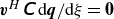
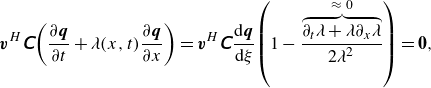 \begin{equation} \boldsymbol{v}^H \unicode{x1D63E} {\left (\frac {\partial \boldsymbol{q}}{\partial t}+\lambda (x,t) \frac {\partial \boldsymbol{q}}{\partial x} \right )}=\boldsymbol{v}^H \unicode{x1D63E} \frac {\text{d}\boldsymbol{q}}{\text{d}\xi } {\left (1-\frac {\overbrace {\partial _t\lambda +\lambda \partial _x \lambda }^{\approx \ 0} }{2\lambda ^2}\right)}={\boldsymbol{0}}, \end{equation}
and a combination of flow variables
 $\boldsymbol{v}^H\unicode{x1D63E} \, \text{d}\boldsymbol{q}/\text{d}\xi = \boldsymbol{0}$
that is conserved to leading order. Note that here the space–time variation of
$\boldsymbol{v}^H\unicode{x1D63E} \, \text{d}\boldsymbol{q}/\text{d}\xi = \boldsymbol{0}$
that is conserved to leading order. Note that here the space–time variation of
 $\lambda$
is assumed to be small compared with that of
$\lambda$
is assumed to be small compared with that of
 $\boldsymbol{q}$
. Therefore, interfacial waves travel ‘freely’ along the characteristic curves defined by
$\boldsymbol{q}$
. Therefore, interfacial waves travel ‘freely’ along the characteristic curves defined by
 $\xi$
with characteristic velocities
$\xi$
with characteristic velocities
 $\lambda$
(simply referred to as `characteristics’).
$\lambda$
(simply referred to as `characteristics’).
In the inhomogeneous case, (3.6) suggests that information is also carried by similar characteristics
 $\lambda$
but with two modifications. Once the viscous stresses are considered the information propagation along the characteristic curves is accompanied by the loss due to a viscous damping effect (momentum loss) or gain due to mixing (thickening of the middle layer) both originating from the
$\lambda$
but with two modifications. Once the viscous stresses are considered the information propagation along the characteristic curves is accompanied by the loss due to a viscous damping effect (momentum loss) or gain due to mixing (thickening of the middle layer) both originating from the
 $\unicode{x1D63F}\kern2pt \boldsymbol{q}$
term. The gravitational forcing due to tilting and geometrical variation in
$\unicode{x1D63F}\kern2pt \boldsymbol{q}$
term. The gravitational forcing due to tilting and geometrical variation in
 $\unicode{x1D63D}\,{\partial \boldsymbol{s}}/{\partial x}$
as well as the non-hydrostatic pressure forcing in
$\unicode{x1D63D}\,{\partial \boldsymbol{s}}/{\partial x}$
as well as the non-hydrostatic pressure forcing in
 $\boldsymbol{\mathcal{F}}$
do not affect the direction of propagation (i.e. modulations) as they do not involve the information content
$\boldsymbol{\mathcal{F}}$
do not affect the direction of propagation (i.e. modulations) as they do not involve the information content
 $\boldsymbol{q}$
. Note that in the inhomogeneous viscous case, there is no conservation of any combination of flow variables along the characteristic curves
$\boldsymbol{q}$
. Note that in the inhomogeneous viscous case, there is no conservation of any combination of flow variables along the characteristic curves
 $\xi$
. Nevertheless, we employ the term `characteristic’, drawing its interpretation from the homogeneous inviscid case.
$\xi$
. Nevertheless, we employ the term `characteristic’, drawing its interpretation from the homogeneous inviscid case.
The preceding analysis assumed a real characteristic velocity
 $\lambda$
. More generally,
$\lambda$
. More generally,
 $\lambda$
may be complex, in which case the interpretation of characteristics must be revisited. As shown in Appendix D, the real part
$\lambda$
may be complex, in which case the interpretation of characteristics must be revisited. As shown in Appendix D, the real part
 $\lambda ^R$
continues to determine the direction of information propagation to leading order, extending the interpretation of real-valued characteristics.
$\lambda ^R$
continues to determine the direction of information propagation to leading order, extending the interpretation of real-valued characteristics.
3.2.1. Analytical solution for the characteristics
The characteristics
 $\lambda$
of the three-layer model are obtained by solving for the eigenvalues in (3.5) that requires
$\lambda$
of the three-layer model are obtained by solving for the eigenvalues in (3.5) that requires
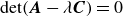 ${\det}(\boldsymbol{A}-\lambda \boldsymbol{C})=0$
for a non-trivial solution leading to the characteristic polynomial
${\det}(\boldsymbol{A}-\lambda \boldsymbol{C})=0$
for a non-trivial solution leading to the characteristic polynomial
 \begin{equation} \sum _{n=0}^{4} a_n \lambda ^n = 0, \end{equation}
with the coefficients
 \begin{align} a_4&=(h_0+\widehat {h}),\nonumber\\ a_3&=-2 \left [\widehat {h} \, u_0 + (u_1 + u_2) h_0+ \widehat {h}\, \widehat {u} \right ],\nonumber \\ a_2 &= \widehat {h} \, {u_0^2 } +4 \widehat {h}\, \widehat {u}\, u_0 + g_1 h_1 (h_0+h_2) \big(F_1^2-1\big) + g_2 h_2 (h_0+h_1) \big(F_2^2-1\big)\nonumber \\ & \quad +4\,h_0 \,u_1 \,u_2, \\ a_1&=-2 \widehat {h}\, \widehat {u} \,{u_0^2 } -2 g_1 h_1 h_2 \big(F_1^2-1\big)\,u_0-2 g_2 h_1 h_2 \big(F_2^2-1\big)\,u_0 -2\,h_0 \,{u_1 } \,u_2 (u_1+u_2)\nonumber \\ & \quad +2 \,h_0 \widehat {h}\, \widehat {u} \, \widehat {g}, \nonumber \\ a_0&={{\det}\; \unicode{x1D63C}}. \nonumber \end{align}
In these coefficients we introduced the height
 $\widehat {h}=h_1+h_2$
, velocity
$\widehat {h}=h_1+h_2$
, velocity
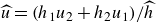 $\widehat {u}=(h_1 u_2 +h_2 u_1)/\widehat {h}$
and reduced gravity
$\widehat {u}=(h_1 u_2 +h_2 u_1)/\widehat {h}$
and reduced gravity
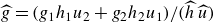 $\widehat {g}=(g_1 h_1 u_2 + g_2 h_2 u_1)/(\widehat {h} \,\widehat {u})$
. We also used the Froude numbers of the bottom, middle and top layers, respectively,
$\widehat {g}=(g_1 h_1 u_2 + g_2 h_2 u_1)/(\widehat {h} \,\widehat {u})$
. We also used the Froude numbers of the bottom, middle and top layers, respectively,
 \begin{eqnarray} F_2=\frac {u_2}{\sqrt { g_2 h_2}}, \quad F_0=\frac {u_0}{\sqrt {\frac {g_1 g_2}{g_1+g_2} h_0}}, \quad F_1=\frac {u_1}{\sqrt {g_1 h_1}}. \end{eqnarray}
The characteristics have the form
 \begin{equation} \begin{aligned} & \lambda _{1}=\,\bar {\!\lambda }-\delta _1\lambda - \delta _2 \lambda ,& \lambda _{2}= \,\bar {\!\lambda }-\delta _1\lambda + \delta _2 \lambda , \nonumber\\[-2pt] & \nonumber \lambda _{3}=\,\bar {\!\lambda }+\delta _1\lambda - \delta _3 \lambda ,& \lambda _{4}=\,\bar {\!\lambda }+\delta _1\lambda + \delta _3 \lambda ,\end{aligned} \end{equation}
where
 $\,\bar {\!\lambda }=-{a_3}/{4a_4}$
is the convective velocity and
$\,\bar {\!\lambda }=-{a_3}/{4a_4}$
is the convective velocity and
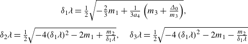 \begin{align} \begin{array}{c} \delta _1\lambda = \frac {1}{2}\sqrt {-\frac {2}{3} m_1 + \frac {1}{3 a_4} \left ( m_3 + \frac {\varDelta _0}{m_3} \right )}, \\ \\[-5pt] \delta _2 \lambda = \frac {1}{2} \sqrt {-4(\delta _1 \lambda )^2-2m_1+\frac {m_2}{\delta _1 \lambda }}, \quad \delta _3 \lambda = \frac {1}{2} \sqrt {-4\left (\delta _1 \lambda \right )^2-2m_1-\frac {m_2}{\delta _1 \lambda }} \end{array} \end{align}
are the phase speeds, where
 \begin{eqnarray} m_1&\!\!=\dfrac {8 a_4 a_2 - 3 a_3^2}{8 a_4^2},\quad m_2=\dfrac {a_3^2-4 a_4 a_3 a_2 + 8 a_4^2 a_1}{8 a_4^3},\quad m_3=\left ( \dfrac {\varDelta _1^2+\sqrt {\varDelta _1^2-4\varDelta _0^3}}{2} \right )^{\tfrac {1}{3}}\!, \quad \nonumber\\[-1.5pt] &&\\[-2.5pt]\nonumber \varDelta _0 &\!\!= a_2^2 - 3 a_3 a_1 + 12 a_4 a_0, \quad \varDelta _1 = 2 a_2^3 - 9 a_3 a_2 a_1 + 27 a_3^2 a_0 + 27 a_4 a_1^2 -72 a_4 a_2 a_0. \end{eqnarray}
Since
 $(\delta _1 \lambda ^R,\delta _2 \lambda ^R,\delta _3 \lambda ^R) \geqslant 0$
, we realise that
$(\delta _1 \lambda ^R,\delta _2 \lambda ^R,\delta _3 \lambda ^R) \geqslant 0$
, we realise that
 $\lambda _1^R \leqslant \lambda _2^R$
,
$\lambda _1^R \leqslant \lambda _2^R$
,
 $\lambda _3^R \leqslant \lambda _4^R$
and
$\lambda _3^R \leqslant \lambda _4^R$
and
 $\lambda _1^R \leqslant \lambda _4^R$
, where the superscript
$\lambda _1^R \leqslant \lambda _4^R$
, where the superscript
 $R$
denotes the real component. Consequently, in a reference frame moving at
$R$
denotes the real component. Consequently, in a reference frame moving at
 $\,\bar {\!\lambda }$
, an observer would see two oppositely propagating interfacial waves, which are associated with the eigenvalues
$\,\bar {\!\lambda }$
, an observer would see two oppositely propagating interfacial waves, which are associated with the eigenvalues
 $\lambda _{1,2}$
and
$\lambda _{1,2}$
and
 $\lambda _{3,4}$
.
$\lambda _{3,4}$
.
To justify this association, we note that the terms
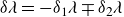 $\delta \lambda = -\delta _1\lambda \mp \delta _2 \lambda$
and
$\delta \lambda = -\delta _1\lambda \mp \delta _2 \lambda$
and
 $\delta \lambda = \delta _1\lambda \mp \delta _3 \lambda$
represent the effective phase speeds of interfacial waves in a three-layer flow. The structure of these expressions suggests that
$\delta \lambda = \delta _1\lambda \mp \delta _3 \lambda$
represent the effective phase speeds of interfacial waves in a three-layer flow. The structure of these expressions suggests that
 $\lambda _{1,2}$
and
$\lambda _{1,2}$
and
 $\lambda _{3,4}$
correspond to long waves propagating along the upper and lower interfaces, respectively. Moreover, since the coefficients in (3.10) are real, if any characteristics become imaginary, they must appear in complex conjugate pairs. Complex conjugate eigenvalues correspond to physically linked interfacial waves, reinforcing the idea that each pair
$\lambda _{3,4}$
correspond to long waves propagating along the upper and lower interfaces, respectively. Moreover, since the coefficients in (3.10) are real, if any characteristics become imaginary, they must appear in complex conjugate pairs. Complex conjugate eigenvalues correspond to physically linked interfacial waves, reinforcing the idea that each pair
 $(\lambda _1, \lambda _2)$
and
$(\lambda _1, \lambda _2)$
and
 $(\lambda _3, \lambda _4)$
can be naturally associated with a single interface. Thus, a key observation from (3.12) is that the eigenvalues
$(\lambda _3, \lambda _4)$
can be naturally associated with a single interface. Thus, a key observation from (3.12) is that the eigenvalues
 $\lambda _{1,2}$
and
$\lambda _{1,2}$
and
 $\lambda _{3,4}$
can be identified with long waves at the upper and lower interfaces, respectively. We note this labelling does not imply that the interfaces are completely decoupled, as their characteristics inherently depend on the velocities and heights of all three layers.
$\lambda _{3,4}$
can be identified with long waves at the upper and lower interfaces, respectively. We note this labelling does not imply that the interfaces are completely decoupled, as their characteristics inherently depend on the velocities and heights of all three layers.
3.2.2. A special case: pure exchange flow with stagnant middle layer
Of particular interest is identifying the conditions under which interfacial waves become unstable. To make progress on this question, we examine a special asymmetric case where
 $u_2 = -u_1$
,
$u_2 = -u_1$
,
 $h_1 = h_2$
and
$h_1 = h_2$
and
 $g_1 = g_2$
. The zero (barotropic) net flow condition implies that
$g_1 = g_2$
. The zero (barotropic) net flow condition implies that
 $u_0=-(u_1 h_1 + u_2 h_2)/h_0=0$
and the coefficient
$u_0=-(u_1 h_1 + u_2 h_2)/h_0=0$
and the coefficient
 $a_3$
vanishes, leading to zero convective velocity (
$a_3$
vanishes, leading to zero convective velocity (
 $\,\bar {\!\lambda }=0$
). This corresponds to the simplest three-layer exchange flow, where the upper and lower layers are symmetric in thickness and stratification, while the middle layer remains stationary. This case is also highly relevant to the SID flow, particularly near the centre of the duct. Under these conditions, the expressions for characteristics in (3.12) simplify significantly (since
$\,\bar {\!\lambda }=0$
). This corresponds to the simplest three-layer exchange flow, where the upper and lower layers are symmetric in thickness and stratification, while the middle layer remains stationary. This case is also highly relevant to the SID flow, particularly near the centre of the duct. Under these conditions, the expressions for characteristics in (3.12) simplify significantly (since
 $F_1 = F_2)$
, yielding
$F_1 = F_2)$
, yielding
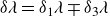
 \begin{equation} \begin{aligned} \lambda _{1,2} &= \mp \frac {\sqrt {g_1 h_1 }}{\sqrt {h_0 +2\,h_1 }}\,\sqrt {h_0\big(1+{F_1^2 }\big)+h_1\big(1-{F_1^2 }\big) - \sigma}, \\ \lambda _{3,4} &= \mp \frac {\sqrt {g_1 h_1 }}{\sqrt {h_0 +2\,h_1 }}\sqrt {h_0\big(1+{F_1^2 }\big)+h_1\big(1-{F_1^2 }\big) +\sigma },\end{aligned} \end{equation}
where
 $\sigma =\sqrt {4 h_0 h_1 {F_1^2 }(1 - {F_1^2 } ) + 4 {h_0^2 } {F_1^2 } +{h_1^2 } (1-{F_1^2 } )^2}$
. Clearly, in this case, if we further restrict the system to
$\sigma =\sqrt {4 h_0 h_1 {F_1^2 }(1 - {F_1^2 } ) + 4 {h_0^2 } {F_1^2 } +{h_1^2 } (1-{F_1^2 } )^2}$
. Clearly, in this case, if we further restrict the system to
 $F_1^2=1$
then
$F_1^2=1$
then
 $\lambda _{1,2}=0$
and
$\lambda _{1,2}=0$
and
 $\lambda _{3,4}=\mp {2 \sqrt {g_1 h_0 h_1}}/{\sqrt {h_0 +2\,h_1}}$
. Since waves in the upper and lower layers become decoupled in this limit, this result supports our approach of associating each eigenvalue pair
$\lambda _{3,4}=\mp {2 \sqrt {g_1 h_0 h_1}}/{\sqrt {h_0 +2\,h_1}}$
. Since waves in the upper and lower layers become decoupled in this limit, this result supports our approach of associating each eigenvalue pair
 $\lambda _{1,2}$
and
$\lambda _{1,2}$
and
 $\lambda _{3,4}$
with a specific interface. However, we note that interfacial waves are coupled where
$\lambda _{3,4}$
with a specific interface. However, we note that interfacial waves are coupled where
 $\,\bar {\!\lambda } \ne 0$
in general.
$\,\bar {\!\lambda } \ne 0$
in general.
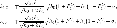
The onset of long-wave instability in the pure exchange flow case visible where (a)
 $\lambda _1^I\gt 0$
and (b)
$\lambda _1^I\gt 0$
and (b)
 $\lambda _4^I\gt 0$
. Here,
$\lambda _4^I\gt 0$
. Here,
 $F$
denotes the Froude number of the upper layer and
$F$
denotes the Froude number of the upper layer and
 $r$
represents the ratio of middle-to-upper/lower layer heights.
$r$
represents the ratio of middle-to-upper/lower layer heights.
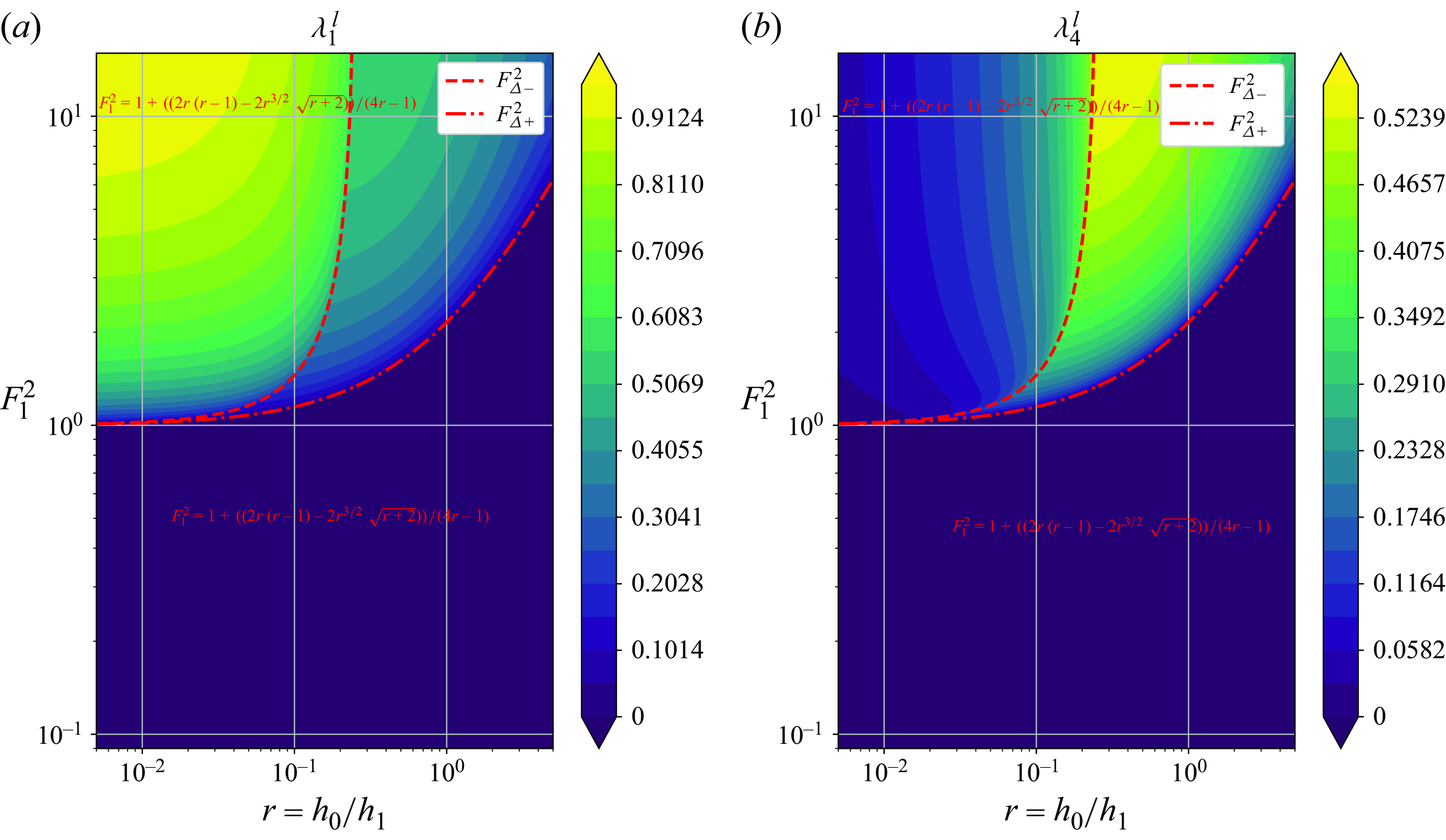
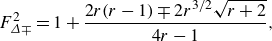
Equation (3.15) reveals that the onset of complex characteristics, indicative of long-wave instability, can be anticipated by identifying the condition under which
 $\sigma$
vanishes. Setting
$\sigma$
vanishes. Setting
 $\sigma = 0$
yields the critical Froude number thresholds
$\sigma = 0$
yields the critical Froude number thresholds
 \begin{equation} F_{\varDelta \mp }^2 = 1 + \frac {2r(r - 1) \mp 2r^{3/2} \sqrt {r + 2}}{4r - 1}, \end{equation}
where
 $r = h_0/h_1$
denotes the ratio of the middle layer depth to the upper (or lower) layer depth. Figure 5 shows
$r = h_0/h_1$
denotes the ratio of the middle layer depth to the upper (or lower) layer depth. Figure 5 shows
 $\lambda _1^I$
and
$\lambda _1^I$
and
 $\lambda _4^I$
as functions of
$\lambda _4^I$
as functions of
 $F_1^2$
for the pure exchange flow. The critical Froude numbers predicted by (3.16) are shown as red dashed lines. We observe that, for
$F_1^2$
for the pure exchange flow. The critical Froude numbers predicted by (3.16) are shown as red dashed lines. We observe that, for
 $F_1^2 \geqslant F_{\varDelta +}^2$
, the characteristics become complex, and the largest values of
$F_1^2 \geqslant F_{\varDelta +}^2$
, the characteristics become complex, and the largest values of
 $\lambda _4^I$
occur within the range
$\lambda _4^I$
occur within the range
 $F_{\varDelta +}^2 \leqslant F_1^2 \leqslant F_{\varDelta -}^2$
. Moreover, the magnitudes of
$F_{\varDelta +}^2 \leqslant F_1^2 \leqslant F_{\varDelta -}^2$
. Moreover, the magnitudes of
 $\lambda _1^I$
and
$\lambda _1^I$
and
 $\lambda _4^I$
change abruptly across the
$\lambda _4^I$
change abruptly across the
 $F_{\varDelta -}^2$
curve. We identify
$F_{\varDelta -}^2$
curve. We identify
 $F_{\varDelta -}^2$
as the bifurcation Froude number and
$F_{\varDelta -}^2$
as the bifurcation Froude number and
 $F_{\varDelta +}^2$
as the marginal-stability Froude number for the pure exchange flow case.
$F_{\varDelta +}^2$
as the marginal-stability Froude number for the pure exchange flow case.
The velocity difference between the upper and middle layers is given by
 $u_1^2 = F_1^2 g_1 h_1$
, since
$u_1^2 = F_1^2 g_1 h_1$
, since
 $u_0 = 0$
in the pure exchange flow. Hence, for
$u_0 = 0$
in the pure exchange flow. Hence, for
 $F_1^2 \geqslant F_{\varDelta +}^2$
, the velocity shear between the upper and middle layers, and between the middle and lower layers, becomes sufficiently strong to trigger long-wave instability on each interface separately. As
$F_1^2 \geqslant F_{\varDelta +}^2$
, the velocity shear between the upper and middle layers, and between the middle and lower layers, becomes sufficiently strong to trigger long-wave instability on each interface separately. As
 $r$
increases, the middle layer thickens relative to the upper layer, causing the upper layer to thin and accelerate. This leads to larger velocity differences across the interfaces, particularly between the faster upper layer and the stagnant middle layer, leading to instability once
$r$
increases, the middle layer thickens relative to the upper layer, causing the upper layer to thin and accelerate. This leads to larger velocity differences across the interfaces, particularly between the faster upper layer and the stagnant middle layer, leading to instability once
 $F_1^2 = F_{\varDelta +}^2$
. This behaviour is analogous to that observed in two-layer flows, where sufficiently strong interfacial shear also leads to long-wave instability.
$F_1^2 = F_{\varDelta +}^2$
. This behaviour is analogous to that observed in two-layer flows, where sufficiently strong interfacial shear also leads to long-wave instability.
The condition
 $\sigma = 0$
corresponds to
$\sigma = 0$
corresponds to
 $\lambda _1 = \lambda _3$
and
$\lambda _1 = \lambda _3$
and
 $\lambda _2 = \lambda _4$
, which implies that the interfacial waves on the lower and upper interfaces have equal phase speeds and can resonate. Instability may therefore arise from this resonance. In the more general case with non-zero convective velocity, however, the identification of instability is less straightforward, a point revisited below and addressed in detail in § 4.
$\lambda _2 = \lambda _4$
, which implies that the interfacial waves on the lower and upper interfaces have equal phase speeds and can resonate. Instability may therefore arise from this resonance. In the more general case with non-zero convective velocity, however, the identification of instability is less straightforward, a point revisited below and addressed in detail in § 4.
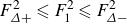
3.2.3. Criticality of interfaces
In a two-layer configuration, the sign of the real component of the characteristics sets the direction of information propagation and the hydraulic regime of the flow, i.e. subcritical, critical or supercritical regime (Long Reference Long1956; Dalziel Reference Dalziel1991; Atoufi et al. Reference Atoufi, Zhu, Lefauve, Taylor, Kerswell, Dalziel, Lawrence and Linden2023). The flow is subcritical when
 $\,\bar {\!\lambda }\lt \delta \lambda ^R$
and information propagates in both leftward (towards decreasing
$\,\bar {\!\lambda }\lt \delta \lambda ^R$
and information propagates in both leftward (towards decreasing
 $x$
) and rightward (towards increasing
$x$
) and rightward (towards increasing
 $x$
) directions, supercritical when
$x$
) directions, supercritical when
 $\,\bar {\!\lambda }\gt \delta \lambda ^R$
and information propagates only either rightward or leftward and critical when
$\,\bar {\!\lambda }\gt \delta \lambda ^R$
and information propagates only either rightward or leftward and critical when
 $\,\bar {\!\lambda }=\delta \lambda ^R$
.
$\,\bar {\!\lambda }=\delta \lambda ^R$
.
In a three-layer configuration, complications arise as the upper and lower layers can individually exhibit different hydraulic regimes. As we found above,
 $\lambda _{1,2}$
and
$\lambda _{1,2}$
and
 $\lambda _{3,4}$
are respectively associated with the upper and lower interface. Therefore, the necessary condition for the upper (respectively lower) layer to be supercritical is
$\lambda _{3,4}$
are respectively associated with the upper and lower interface. Therefore, the necessary condition for the upper (respectively lower) layer to be supercritical is
 $\lambda _1^R \lambda _2^R \gt 0$
(respectively
$\lambda _1^R \lambda _2^R \gt 0$
(respectively
 $\lambda _3^R \lambda _4^R \gt 0$
). Information on each interface thus propagates in a particular direction, depending on the signs of the characteristics (Sannino et al. Reference Sannino, Carillo and Artale2007, Reference Sannino, Pratt and Carillo2009).
$\lambda _3^R \lambda _4^R \gt 0$
). Information on each interface thus propagates in a particular direction, depending on the signs of the characteristics (Sannino et al. Reference Sannino, Carillo and Artale2007, Reference Sannino, Pratt and Carillo2009).
The characteristic pairs
 $\lambda _1^R \lambda _2^R$
and
$\lambda _1^R \lambda _2^R$
and
 $\lambda _3^R \lambda _4^R$
determine criticality with respect to the individual layers, not the full three-layer system. For example, the flow may be supercritical in both layers if
$\lambda _3^R \lambda _4^R$
determine criticality with respect to the individual layers, not the full three-layer system. For example, the flow may be supercritical in both layers if
 $\lambda _1^R \lambda _2^R \gt 0$
and
$\lambda _1^R \lambda _2^R \gt 0$
and
 $\lambda _3^R \lambda _4^R \gt 0$
, yet remain subcritical overall, e.g. if
$\lambda _3^R \lambda _4^R \gt 0$
, yet remain subcritical overall, e.g. if
 $\lambda _1^R, \lambda _2^R \lt 0$
and
$\lambda _1^R, \lambda _2^R \lt 0$
and
 $\lambda _3^R, \lambda _4^R \gt 0$
. The three-layer flow is fully supercritical only when all layers are hydraulically supercritical and the corresponding characteristics have the same sign, so that information propagates in a single direction. It is fully subcritical when all layers are subcritical, or when the layers are supercritical but the characteristic signs differ, indicating opposing directions of information propagation. A critical condition arises when at least one characteristic pair satisfies
$\lambda _3^R, \lambda _4^R \gt 0$
. The three-layer flow is fully supercritical only when all layers are hydraulically supercritical and the corresponding characteristics have the same sign, so that information propagates in a single direction. It is fully subcritical when all layers are subcritical, or when the layers are supercritical but the characteristic signs differ, indicating opposing directions of information propagation. A critical condition arises when at least one characteristic pair satisfies
 $\lambda _i^R \lambda _j^R = 0$
, at which point information propagation is blocked and internal hydraulic control is established.
$\lambda _i^R \lambda _j^R = 0$
, at which point information propagation is blocked and internal hydraulic control is established.
3.2.4. Critical middle layer thickness
The emergence of imaginary components, as conjugate pairs, in the characteristics implies the onset of instability of long waves as established in Appendix A. Consequently, we can predict critical values of the layer velocities and heights that cause interfaces to be unstable to disturbances of the given wavenumber
 $k$
by examining the coefficients
$k$
by examining the coefficients
 $b_i$
of the quartic stability equation (A10) given below,
$b_i$
of the quartic stability equation (A10) given below,
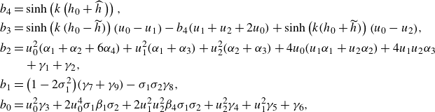 \begin{align} b_4 &= \sinh \left (k\,{\left (h_0 +\widehat {h} {\kern2pt}\right )}\right ), \nonumber\\ b_3&=\sinh \left (k\,(h_0-\widetilde {h})\right ){\left (u_0 -u_1 \right )}- b_4 (u_1+u_2+2 u_0) + \sinh \left (k (h_0+\widetilde {h})\right ){\left (u_0 -u_2 \right )}, \nonumber\\ b_2 &= u_0^2 (\alpha _1 + \alpha _2 + 6 \alpha _4) + u_1^2 (\alpha _1 + \alpha _3) + u_2^2 (\alpha _2 + \alpha _3) + 4 u_0 (u_1 \alpha _1 + u_2 \alpha _2) + 4 u_1 u_2 \alpha _3 \nonumber \\ & \quad + \gamma _1 + \gamma _2, \\ b_1 &= \big(1 - 2 \sigma _1^2\big)(\gamma _{7} + \gamma _9) - \sigma _1 \sigma _2 \gamma _{8}, \nonumber\\ b_0 &= u_0^2 \gamma _3 + 2 u_0^4 \sigma _1 \beta _1 \sigma _2 + 2 u_1^2 u_2^2 \beta _4 \sigma _1 \sigma _2 + u_2^2 \gamma _4 + u_1^2 \gamma _5 + \gamma _6,\nonumber \end{align}
and to long waves by examining
 $a_i$
in (3.10) where
$a_i$
in (3.10) where
 $\widetilde {h}={h_1-h_2}$
and
$\widetilde {h}={h_1-h_2}$
and
 $\alpha _i, \sigma _i$
and
$\alpha _i, \sigma _i$
and
 $\gamma _i$
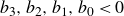
are defined in Appendix A.1. For example, the necessary condition guaranteeing only real roots is that
$\gamma _i$
are defined in Appendix A.1. For example, the necessary condition guaranteeing only real roots is that
 $b_i$
should be all positive or all negative (based on the Routh–Hurwitz stability criterion (Shinners Reference Shinners1998). As wavenumbers
$b_i$
should be all positive or all negative (based on the Routh–Hurwitz stability criterion (Shinners Reference Shinners1998). As wavenumbers
 $k \geqslant 0$
, then
$k \geqslant 0$
, then
 $b_4 \geqslant 0$
and this condition leads to one of the
$b_4 \geqslant 0$
and this condition leads to one of the
 $b_3, b_2, b_1, b_0 \lt 0$
for all
$b_3, b_2, b_1, b_0 \lt 0$
for all
 $k$
for instability to happen.
$k$
for instability to happen.
In fact, the number of sign changes in
 $b_i$
yields the number of complex roots and potential instability. As
$b_i$
yields the number of complex roots and potential instability. As
 $\lambda$
(i.e. the long-wave limit of the phase speed
$\lambda$
(i.e. the long-wave limit of the phase speed
 $c$
of disturbance waves) appears in the form of complex conjugates, there are four complex roots and
$c$
of disturbance waves) appears in the form of complex conjugates, there are four complex roots and
 $a_{3,2,1,0}$
change sign (note
$a_{3,2,1,0}$
change sign (note
 $a_4$
is constant inside the duct). In the limit of long waves, using the
$a_4$
is constant inside the duct). In the limit of long waves, using the
 $b_3=a_3 \lt 0$
condition and incorporating the zero net flow condition
$b_3=a_3 \lt 0$
condition and incorporating the zero net flow condition
 $Q=u_0 h_0 + u_1 h_1 + u_2 h_2 = 0$
to eliminate
$Q=u_0 h_0 + u_1 h_1 + u_2 h_2 = 0$
to eliminate
 $u_0$
in
$u_0$
in
 $a_3$
yields a restriction for the height of the middle layer that
$a_3$
yields a restriction for the height of the middle layer that
 $ -{2{(h_0 +\widehat {h})}{ (h_0 (u_1 + u_2) -h_1 u_1 -h_2 u_2 )}}/{h_0 } \lt 0$
for instability to occur.
$ -{2{(h_0 +\widehat {h})}{ (h_0 (u_1 + u_2) -h_1 u_1 -h_2 u_2 )}}/{h_0 } \lt 0$
for instability to occur.
This leads to
 \begin{equation} h_0^{cr}=\frac {u_1 h_1 + u_2 h_2}{u_1 + u_2} \end{equation}
as the critical height for the middle layer. Therefore, when
 $u_2 \lt {\lvert {u_1} \rvert }$
(i.e. an interface with a positive slope) and
$u_2 \lt {\lvert {u_1} \rvert }$
(i.e. an interface with a positive slope) and
 $h_0 \gt h_0^{cr}$
, the three-layer exchange flow is become unstable to long waves and may be supercritical. In the limit of short waves, where
$h_0 \gt h_0^{cr}$
, the three-layer exchange flow is become unstable to long waves and may be supercritical. In the limit of short waves, where
 $k \gg 1$
, the sign of
$k \gg 1$
, the sign of
 $b_3$
depends on the coefficients of the largest
$b_3$
depends on the coefficients of the largest
 $k$
(positive) when expanding
$k$
(positive) when expanding
 $b_3$
with respect to
$b_3$
with respect to
 $k$
. Specifically, when
$k$
. Specifically, when
 $u_2 h_0 + u_1 h_1 + u_2 h_2 \gt 0$
, we have
$u_2 h_0 + u_1 h_1 + u_2 h_2 \gt 0$
, we have
 $b_3 \lt 0$
, satisfying the necessary condition. This leads to the condition
$b_3 \lt 0$
, satisfying the necessary condition. This leads to the condition
 $h_0 \gt {(|u_1| h_1 - u_2 h_2)}/{u_2}$
, which provides a smaller lower bound for
$h_0 \gt {(|u_1| h_1 - u_2 h_2)}/{u_2}$
, which provides a smaller lower bound for
 $h_0$
and a smaller critical middle layer thickness than in (3.18). Therefore, it is expected that short waves will become unstable first. Nonetheless, it is the long waves (hydraulic effects) that set the interface slopes, and thus, the upper and lower layer flow rates
$h_0$
and a smaller critical middle layer thickness than in (3.18). Therefore, it is expected that short waves will become unstable first. Nonetheless, it is the long waves (hydraulic effects) that set the interface slopes, and thus, the upper and lower layer flow rates
 $u_1 h_1$
and
$u_1 h_1$
and
 $u_2 h_2$
, which then determine the value of
$u_2 h_2$
, which then determine the value of
 $h_0$
that results in
$h_0$
that results in
 $b_3 \lt 0$
and the onset of the short-wave instabilities.
$b_3 \lt 0$
and the onset of the short-wave instabilities.
3.2.5. Application to the data
The three-layer model, yielding layer characteristics, is applied to the layer-averaged DNS data in figure 6. The space–time evolution of
 $\lambda _1$
and
$\lambda _1$
and
 $\lambda _3$
in the TW case are shown with
$\lambda _3$
in the TW case are shown with
 $x{-}t$
plots. The dashed lines are reproduced from the layer-averaged quantities in figure 3, indicating the drastic changes in the layer statistics. Noticeably, the left and right lines are, respectively, in alignment with
$x{-}t$
plots. The dashed lines are reproduced from the layer-averaged quantities in figure 3, indicating the drastic changes in the layer statistics. Noticeably, the left and right lines are, respectively, in alignment with
 $\lambda _1^R$
and
$\lambda _1^R$
and
 $\lambda _3^R\approx 0$
, which indicates the emergence of critical points in the upper and lower layer interfaces. The flow becomes critical on these lines, which is also evidenced by the appearance of hydraulic jumps as illustrated by the sudden changes of the corresponding layer heights in figure 3. In addition, the three-layer model predicts one control point near the inlet/outlet of the duct due to geometry changes, which agrees with the two-layer model in Atoufi et al. (Reference Atoufi, Zhu, Lefauve, Taylor, Kerswell, Dalziel, Lawrence and Linden2023).
$\lambda _3^R\approx 0$
, which indicates the emergence of critical points in the upper and lower layer interfaces. The flow becomes critical on these lines, which is also evidenced by the appearance of hydraulic jumps as illustrated by the sudden changes of the corresponding layer heights in figure 3. In addition, the three-layer model predicts one control point near the inlet/outlet of the duct due to geometry changes, which agrees with the two-layer model in Atoufi et al. (Reference Atoufi, Zhu, Lefauve, Taylor, Kerswell, Dalziel, Lawrence and Linden2023).
Selected eigenvalues of the three-layer model for the TW case (
 $\textit{Re} = 650, \theta = 6^\circ$
): (a,d) real and imaginary components of the characteristic
$\textit{Re} = 650, \theta = 6^\circ$
): (a,d) real and imaginary components of the characteristic
 $\lambda _1$
for the upper interface, (b,e)
$\lambda _1$
for the upper interface, (b,e)
 $\lambda _3$
for the lower interface and (c,f) product of the real and imaginary components of
$\lambda _3$
for the lower interface and (c,f) product of the real and imaginary components of
 $\lambda _1$
and
$\lambda _1$
and
 $\lambda _3$
. The dashed and dash-dotted lines correspond to those in figure 3.
$\lambda _3$
. The dashed and dash-dotted lines correspond to those in figure 3.

In figure 6(c), outside of the critical lines, the real components of the characteristics have the same sign and are positive/negative on the left/right side of the duct, respectively. Therefore, the information of the three-layer system can only propagate from the critical point near the inlet/outlet toward the duct centre. In between the critical lines,
 $\lambda _1^R\lambda _3^R\lt 0$
and the flow is subcritical. Waves in this region can propagate in either direction. This region is where the thickening of the middle layer occurs (see figure 3).
$\lambda _1^R\lambda _3^R\lt 0$
and the flow is subcritical. Waves in this region can propagate in either direction. This region is where the thickening of the middle layer occurs (see figure 3).
The imaginary components of characteristics correspond to the growth rate of the long interfacial waves (as discussed in Appendix A). As indicated by figure 6(d,e), the long waves at the upper interface become unstable (
 $\lambda _1^I\gt 0$
) in the left and middle regions of the duct, whereas the long waves at the lower interface are unstable in the middle and right regions (
$\lambda _1^I\gt 0$
) in the left and middle regions of the duct, whereas the long waves at the lower interface are unstable in the middle and right regions (
 $\lambda _3^I \gt 0$
) where the superscript I refers to the imaginary component of
$\lambda _3^I \gt 0$
) where the superscript I refers to the imaginary component of
 $\lambda$
. While the stability of individual interfaces can be deduced from the associated characteristics, the stability of the three-layer flow system is less straightforward and requires consideration of resonance between interfaces, which will be discussed in § 4.
$\lambda$
. While the stability of individual interfaces can be deduced from the associated characteristics, the stability of the three-layer flow system is less straightforward and requires consideration of resonance between interfaces, which will be discussed in § 4.
Instantaneous characteristics of the interfacial waves on the upper and lower interfaces in DNS, diagnosed using the three-layer hydraulic analysis. The real components of the characteristics, representing the phase speed of the upper and lower interfacial waves (
 $\lambda _1^R$
and
$\lambda _1^R$
and
 $\lambda _3^R$
), are shown in (a,c). The imaginary components, representing the growth rate of the upper and lower interfacial waves (
$\lambda _3^R$
), are shown in (a,c). The imaginary components, representing the growth rate of the upper and lower interfacial waves (
 $\lambda _1^I$
and
$\lambda _1^I$
and
 $\lambda _3^I$
), are shown in (b,d).
$\lambda _3^I$
), are shown in (b,d).
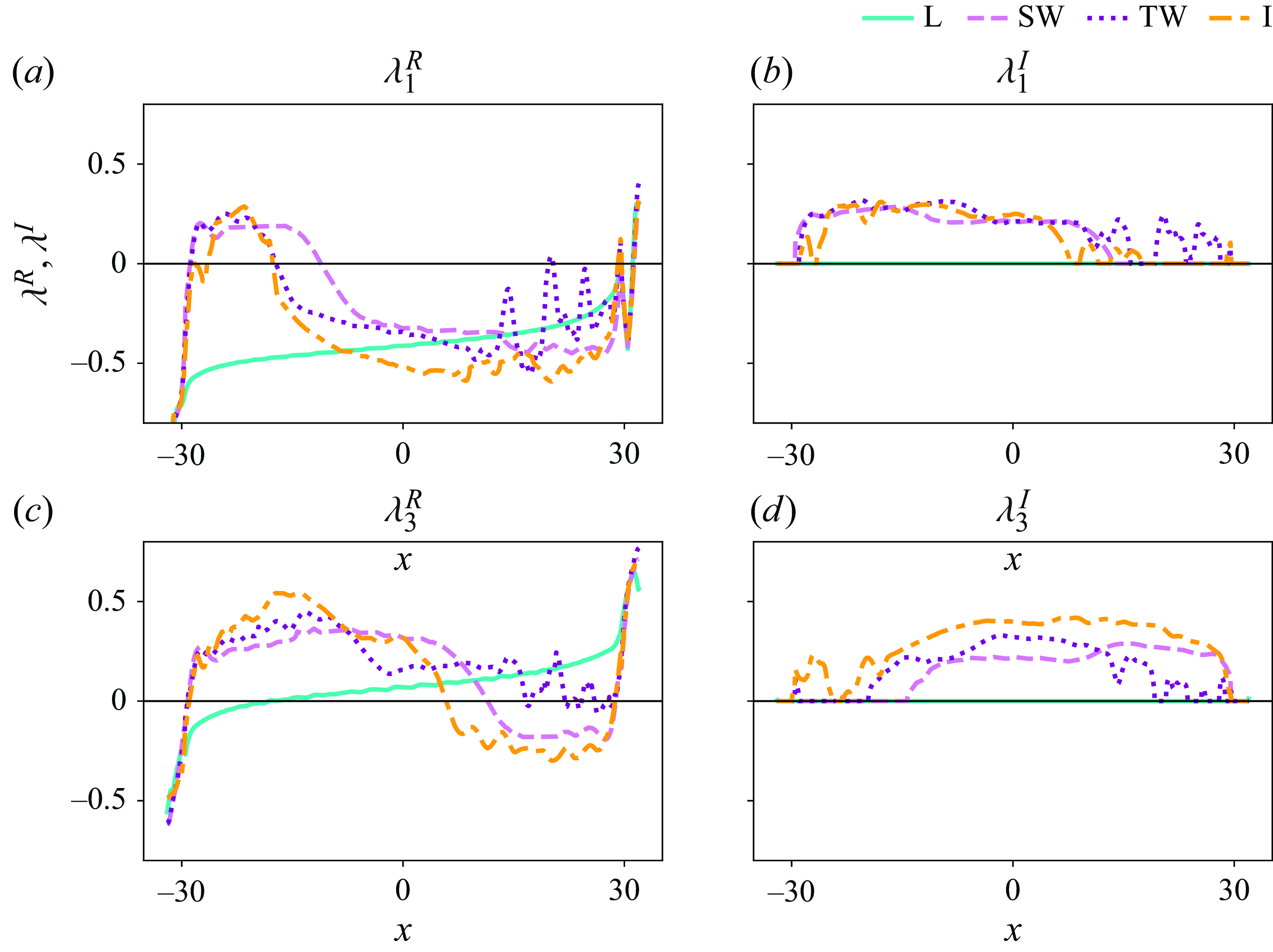
The real and imaginary components of the instantaneous characteristics are shown in figure 7 at
 $t = 120$
for the L, SW, TW and I cases, to complement the space–time distribution of the characteristics, which was previously given only for the TW case. The instantaneous
$t = 120$
for the L, SW, TW and I cases, to complement the space–time distribution of the characteristics, which was previously given only for the TW case. The instantaneous
 $\lambda ^R$
and
$\lambda ^R$
and
 $\lambda ^I$
of all non-laminar cases follow a similar trend. The imaginary component in figure 7(b,d) shows that in the L case,
$\lambda ^I$
of all non-laminar cases follow a similar trend. The imaginary component in figure 7(b,d) shows that in the L case,
 $\lambda ^I \approx 0$
for both the upper and lower interfaces, whereas in the SW, TW and I cases,
$\lambda ^I \approx 0$
for both the upper and lower interfaces, whereas in the SW, TW and I cases,
 $\lambda _1^I, \lambda _3^I \gt 0$
in most places inside the duct.
$\lambda _1^I, \lambda _3^I \gt 0$
in most places inside the duct.
The application of the three-layer theory to the DNS data suggests that three-layer characteristics are not only useful in quantifying information propagation but also in informing us about regions where turbulence and mixing occur. We detail this connection between characteristics and turbulence next.
3.3. Hydraulic regime transitions and turbulence
Here we identify an equivalent Froude number of a three-layer flow that predicts hydraulic regime transition and control in a three-layer exchange flow in § 3.3.2. Then, we use this three-layer Froude number to show how hydraulic control leads to turbulence generation in § 3.3.3.
3.3.1. Critical exchange flow regime
To define hydraulic control, we use the steady-state solution of (3.1). For
 $\boldsymbol{\mathcal{F}}=0$
, the steady solution of (3.1) can be found by multiplying the inverse matrix
$\boldsymbol{\mathcal{F}}=0$
, the steady solution of (3.1) can be found by multiplying the inverse matrix
 $\unicode{x1D63C}^{-1}={\rm adj} (\unicode{x1D63C})/{\det}\; \unicode{x1D63C}$
on both sides leading to
$\unicode{x1D63C}^{-1}={\rm adj} (\unicode{x1D63C})/{\det}\; \unicode{x1D63C}$
on both sides leading to
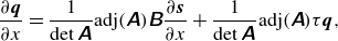 \begin{equation} \frac {\partial \boldsymbol{q}}{\partial x}=\frac {1}{{\det}\; \unicode{x1D63C}} {\rm adj} (\unicode{x1D63C}) \unicode{x1D63D}\frac {\partial \boldsymbol{s}}{\partial x}+\frac {1}{{\det}\; \unicode{x1D63C}} {\rm adj} (\unicode{x1D63C}) {\tau } \boldsymbol{q}, \end{equation}
where
 ${\rm adj} (\unicode{x1D63C})$
represent the transpose of the co-factor matrix of
${\rm adj} (\unicode{x1D63C})$
represent the transpose of the co-factor matrix of
 $\unicode{x1D63C}$
. A non-trivial steady solution
$\unicode{x1D63C}$
. A non-trivial steady solution
 $\boldsymbol{q}(x)$
of (3.1) requires
$\boldsymbol{q}(x)$
of (3.1) requires
 \begin{equation} {\det}\; \unicode{x1D63C}= g_1 g_2 h_1 h_0 h_2 ({G}-1) \ne 0, \end{equation}
where
 $G$
is the composite Froude number defined based on the individual layers
$G$
is the composite Froude number defined based on the individual layers
 \begin{equation} {G}=1+{\big (\epsilon _1 {F_1^2 } + \epsilon _2 {F_2^2 } -1\big )}\,{F_0^2 } +{\big ({F_1^2 } -1\big )}\,{\big ({F_2^2 } -1\big )}, \end{equation}
where
 $\epsilon _1=g_1/(g_1+g_2)$
,
$\epsilon _1=g_1/(g_1+g_2)$
,
 $\epsilon _2=g_2/(g_1+g_2)$
are the ratio of cross-interface to total density differences.
$\epsilon _2=g_2/(g_1+g_2)$
are the ratio of cross-interface to total density differences.
The three-layer flow is hydraulically controlled when
 $h_0=0$
or
$h_0=0$
or
 ${G}=1$
(i.e.
${G}=1$
(i.e.
 ${\det}\; \unicode{x1D63C}=0$
). The condition
${\det}\; \unicode{x1D63C}=0$
). The condition
 $h_0=0$
is trivial as it removes the third layer. Generally, the hydraulic control condition incorporating (3.21) defines a critical state in the three-layer exchange flow, where
$h_0=0$
is trivial as it removes the third layer. Generally, the hydraulic control condition incorporating (3.21) defines a critical state in the three-layer exchange flow, where
 \begin{equation} F_0^2=\frac {\left(F_1^2-1\right)\left(F_2^2-1\right)}{\left(1- \epsilon _1 F_1^2 - \epsilon _2 F_2^2\right)}, \end{equation}
yielding
 $G=1$
. This equation imposes a fundamental constraint on the middle layer, determining its velocity and thickness based on the Froude numbers of the upper and lower layers, thereby fully characterising its dynamics under hydraulic control. Determining whether a three-layer exchange flow beyond the critical state is subcritical or supercritical requires linking (3.21) to the characteristics of long interfacial waves, as discussed in the next section. Nonetheless, (3.22) allows the exploration of the possible combinations of supercritical and subcritical flows in each layer even though the overall three-layer system remains in a critical state. Figure 8(a) shows the middle layer Froude number
$G=1$
. This equation imposes a fundamental constraint on the middle layer, determining its velocity and thickness based on the Froude numbers of the upper and lower layers, thereby fully characterising its dynamics under hydraulic control. Determining whether a three-layer exchange flow beyond the critical state is subcritical or supercritical requires linking (3.21) to the characteristics of long interfacial waves, as discussed in the next section. Nonetheless, (3.22) allows the exploration of the possible combinations of supercritical and subcritical flows in each layer even though the overall three-layer system remains in a critical state. Figure 8(a) shows the middle layer Froude number
 $F_0^2$
at the critical state, computed from (3.21) for
$F_0^2$
at the critical state, computed from (3.21) for
 $\epsilon _1 = \epsilon _2 = 0.5$
, as a function of
$\epsilon _1 = \epsilon _2 = 0.5$
, as a function of
 $F_1^2$
and
$F_1^2$
and
 $F_2^2$
. The structure is similar to figure 3 in Sannino, Pratt & Carillo (Reference Sannino, Pratt and Carillo2009), based on a three-layer model for the Strait of Gibraltar. Figure 8(b) shows the corresponding contour plot in the
$F_2^2$
. The structure is similar to figure 3 in Sannino, Pratt & Carillo (Reference Sannino, Pratt and Carillo2009), based on a three-layer model for the Strait of Gibraltar. Figure 8(b) shows the corresponding contour plot in the
 $F_1^2$
–
$F_1^2$
–
 $F_2^2$
plane. Following Sannino et al. (Reference Sannino, Pratt and Carillo2009), Sánchez-Garrido et al. (Reference Sánchez-Garrido, Sannino, Liberti, García Lafuente and Pratt2011), four distinct regimes are identified and labelled using the notation
$F_2^2$
plane. Following Sannino et al. (Reference Sannino, Pratt and Carillo2009), Sánchez-Garrido et al. (Reference Sánchez-Garrido, Sannino, Liberti, García Lafuente and Pratt2011), four distinct regimes are identified and labelled using the notation
 $(F_1^2, F_2^2, F_0^2)$
, where each symbol (
$(F_1^2, F_2^2, F_0^2)$
, where each symbol (
 $\gt$
or
$\gt$
or
 $\lt$
) denotes whether the corresponding layer is hydraulically supercritical or subcritical relative to the others. These labels illustrate how individual layers may exhibit distinct hydraulic states, even though the overall flow remains critical. For instance,
$\lt$
) denotes whether the corresponding layer is hydraulically supercritical or subcritical relative to the others. These labels illustrate how individual layers may exhibit distinct hydraulic states, even though the overall flow remains critical. For instance,
 $(\gt ,\lt ,\gt )$
represents a critical regime where the upper and middle layers are supercritical, while the lower layer is subcritical. Sannino et al. (Reference Sannino, Pratt and Carillo2009) referred to the region marked
$(\gt ,\lt ,\gt )$
represents a critical regime where the upper and middle layers are supercritical, while the lower layer is subcritical. Sannino et al. (Reference Sannino, Pratt and Carillo2009) referred to the region marked
 $(\lt ,\lt ,\lt )$
as a provisionally subcritical regime, in which all layers are subcritical and wave motions in the upper and lower layers are coupled. They referred to the region
$(\lt ,\lt ,\lt )$
as a provisionally subcritical regime, in which all layers are subcritical and wave motions in the upper and lower layers are coupled. They referred to the region
 $(\gt ,\gt ,\lt )$
as a provisionally supercritical regime, where the upper and lower layers are supercritical while the middle layer remains subcritical.
$(\gt ,\gt ,\lt )$
as a provisionally supercritical regime, where the upper and lower layers are supercritical while the middle layer remains subcritical.
Critical state of the exchange flow. (a) Surface plot of the middle layer Froude number
 $F_0^2$
as a function of the upper layer (
$F_0^2$
as a function of the upper layer (
 $F_1^2$
) and lower layer (
$F_1^2$
) and lower layer (
 $F_2^2$
) Froude numbers, satisfying the critical condition given in (3.22). (b) Contour plot of the same critical surface, showing level curves of
$F_2^2$
) Froude numbers, satisfying the critical condition given in (3.22). (b) Contour plot of the same critical surface, showing level curves of
 $F_0^2$
in the
$F_0^2$
in the
 $F_1^2$
–
$F_1^2$
–
 $F_2^2$
plane. Regions are labelled using triple inequality notation (e.g.
$F_2^2$
plane. Regions are labelled using triple inequality notation (e.g.
 $\gt ,\lt ,\lt$
), indicating whether each layer is supercritical or subcritical relative to the others. These combinations illustrate how individual layers may depart from criticality, while the overall three-layer flow remains in a critical state.
$\gt ,\lt ,\lt$
), indicating whether each layer is supercritical or subcritical relative to the others. These combinations illustrate how individual layers may depart from criticality, while the overall three-layer flow remains in a critical state.
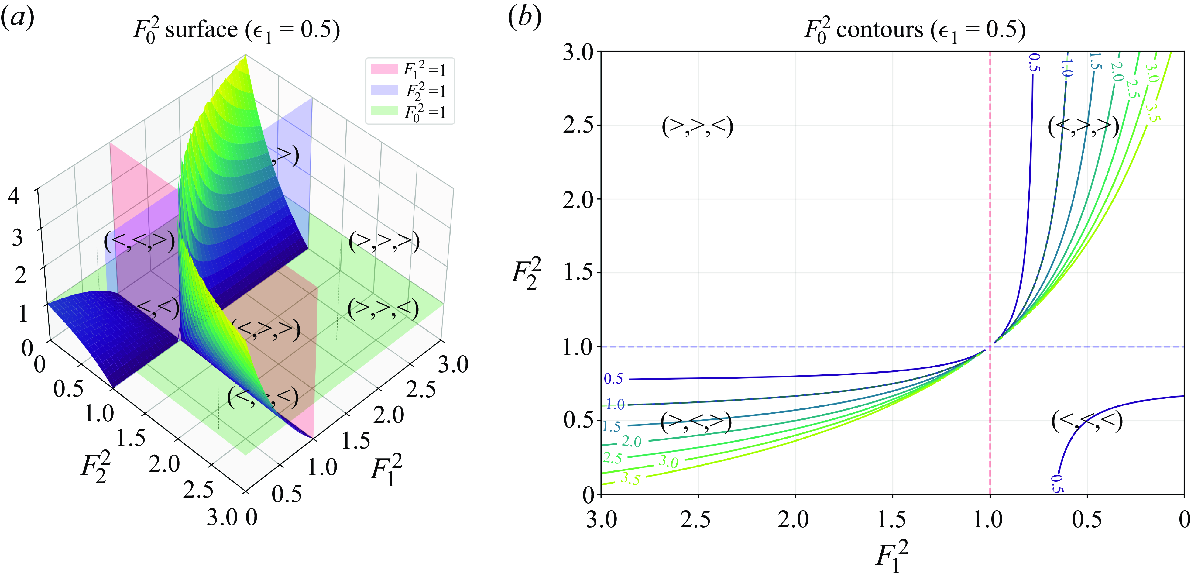
In the special case where the middle layer is stagnant (
 $u_0 = 0$
, so that
$u_0 = 0$
, so that
 $F_0 = 0$
) and either the upper layer or lower layer Froude number reaches unity, i.e.
$F_0 = 0$
) and either the upper layer or lower layer Froude number reaches unity, i.e.
 ${\lvert {F_1} \rvert } = 1$
or
${\lvert {F_1} \rvert } = 1$
or
 ${\lvert {F_2} \rvert } = 1$
, a hydraulically controlled region emerges – bounded by
${\lvert {F_2} \rvert } = 1$
, a hydraulically controlled region emerges – bounded by
 ${\lvert {F_1} \rvert } = 1$
or
${\lvert {F_1} \rvert } = 1$
or
 ${\lvert {F_2}\rvert } = 1$
– in contrast to the localised control points typically found in two-layer flows (Atoufi et al. Reference Atoufi, Zhu, Lefauve, Taylor, Kerswell, Dalziel, Lawrence and Linden2023).
${\lvert {F_2}\rvert } = 1$
– in contrast to the localised control points typically found in two-layer flows (Atoufi et al. Reference Atoufi, Zhu, Lefauve, Taylor, Kerswell, Dalziel, Lawrence and Linden2023).
To extend this classification beyond the critical state, the characteristics must be related to a composite Froude number
 $G$
, as introduced in the following section, that reflects the direction of information propagation.
$G$
, as introduced in the following section, that reflects the direction of information propagation.
3.3.2. Three-layer hydraulic regimes identifier
The link between characteristics and
 $G$
can be highlighted by noting
$G$
can be highlighted by noting
 $\Pi _{i=1}^4 \lambda _i = {a_0}/{a_4}$
combined with (3.20), yielding the identity
$\Pi _{i=1}^4 \lambda _i = {a_0}/{a_4}$
combined with (3.20), yielding the identity
 \begin{eqnarray} {G} = 1 + \dfrac {(h_1 + h_0 + h_2)}{g_1 g_2 h_1 h_0 h_2} \Pi _{i=1}^4 \lambda _i. \end{eqnarray}
Although the condition
 $G=1$
in a three-layer flow can be used to identify control points, neither (3.21) nor (3.23) can provide insights into whether the three-layer flow is subcritical or supercritical. The reason is that when characteristic speeds of long interfacial waves at both interfaces have imaginary components, the multiplication of all complex characteristic speeds mixes up information propagation associated with each interface and typically gives
$G=1$
in a three-layer flow can be used to identify control points, neither (3.21) nor (3.23) can provide insights into whether the three-layer flow is subcritical or supercritical. The reason is that when characteristic speeds of long interfacial waves at both interfaces have imaginary components, the multiplication of all complex characteristic speeds mixes up information propagation associated with each interface and typically gives
 $G \geqslant 1$
. As only the real components of the characteristics determine the hydraulic regimes (imaginary components quantify the long-wave growth rate, as shown in Appendix A), based on the definition of
$G \geqslant 1$
. As only the real components of the characteristics determine the hydraulic regimes (imaginary components quantify the long-wave growth rate, as shown in Appendix A), based on the definition of
 $G$
, we define a modified composite Froude number
$G$
, we define a modified composite Froude number
 \begin{eqnarray} \widetilde {G}=1+ \dfrac {(h_1+h_0+h_2)}{g_1 g_2 h_1 h_0 h_2} \textrm{sign}{\big(\lambda ^R_1 \lambda ^R_4\big )} \Pi _{i=1}^4 \lambda ^R_i \end{eqnarray}
that is capable of identifying hydraulic regimes in three-layer flows with complex characteristics. Note that
 $\widetilde {G}$
can be negative, and
$\widetilde {G}$
can be negative, and
 $\widetilde {G}=1$
at control points, but generally
$\widetilde {G}=1$
at control points, but generally
 $G \geqslant \widetilde {G}$
. When the real components of the four characteristics have the same sign, then
$G \geqslant \widetilde {G}$
. When the real components of the four characteristics have the same sign, then
 $\widetilde {G}\gt 1$
, indicating a supercritical regime. Conversely, when
$\widetilde {G}\gt 1$
, indicating a supercritical regime. Conversely, when
 $\widetilde {G}\lt 1$
, the real components have opposite signs, indicating a subcritical regime. The condition
$\widetilde {G}\lt 1$
, the real components have opposite signs, indicating a subcritical regime. The condition
 $\widetilde {G}=1$
indicates critical flow since the real component of the characteristic associated with one of the interfaces vanishes.
$\widetilde {G}=1$
indicates critical flow since the real component of the characteristic associated with one of the interfaces vanishes.
(a–c) Normalised TKE
 $k^\prime _m/\langle k^\prime _m\rangle _{\mathcal{V},t}$
averaged over the duct cross-section (
$k^\prime _m/\langle k^\prime _m\rangle _{\mathcal{V},t}$
averaged over the duct cross-section (
 $\langle \cdot \rangle _{\mathcal{V},t}$
denotes the spatial and temporal average). (d–f) Modified composite Froude number for the three-layer model,
$\langle \cdot \rangle _{\mathcal{V},t}$
denotes the spatial and temporal average). (d–f) Modified composite Froude number for the three-layer model,
 $\widetilde {G}$
, as defined in (3.24). (g–i) Modified composite Froude number for the two-layer model,
$\widetilde {G}$
, as defined in (3.24). (g–i) Modified composite Froude number for the two-layer model,
 $\widetilde {G}^{2L}$
, as defined in (3.28). The first row represents the SW case, the second row represents the TW case and the third row represents the I case. The dashed and dashed-dotted green curves are identical to those in figure 3.
$\widetilde {G}^{2L}$
, as defined in (3.28). The first row represents the SW case, the second row represents the TW case and the third row represents the I case. The dashed and dashed-dotted green curves are identical to those in figure 3.
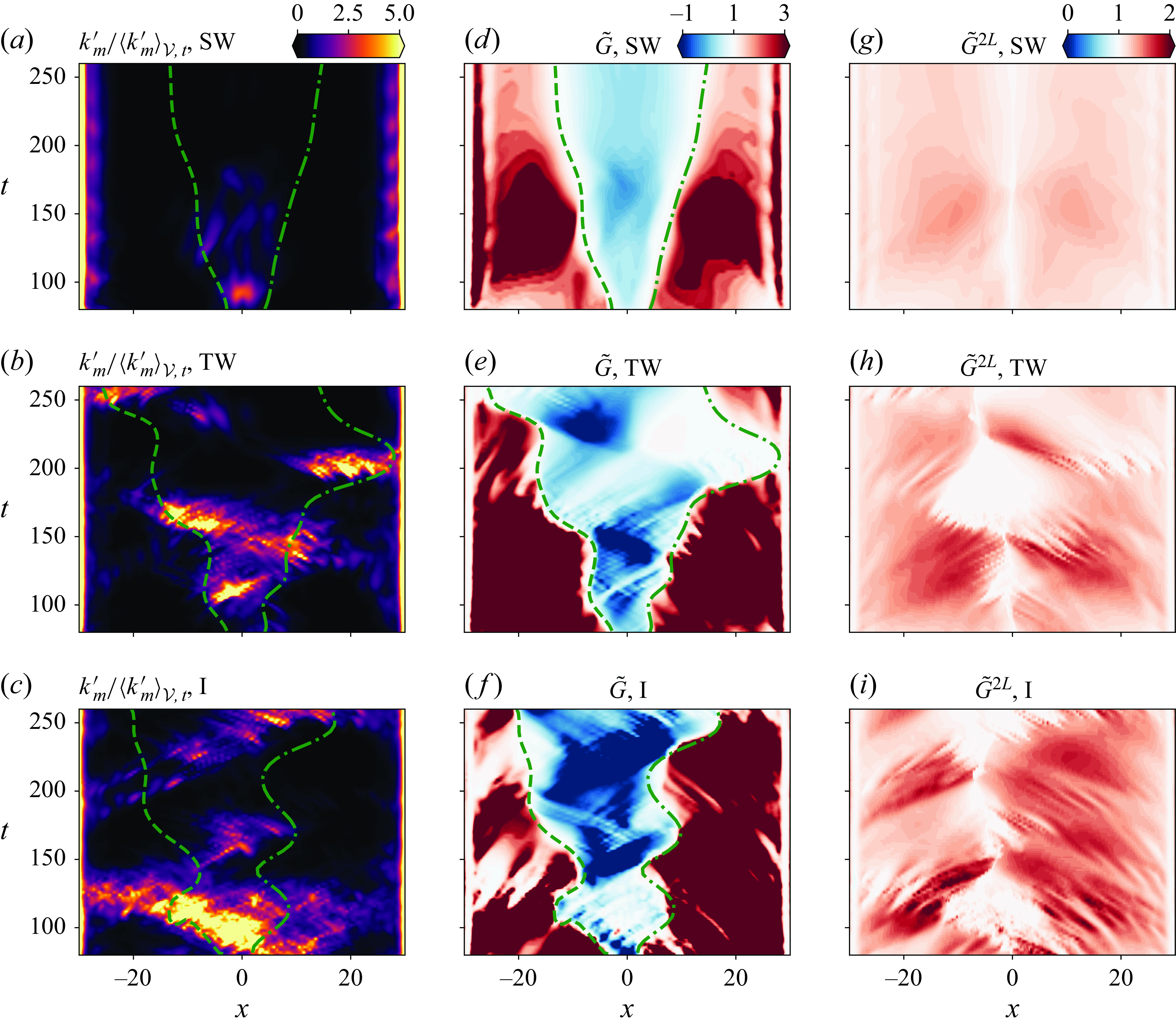
Thus,
 $\widetilde {G}$
provides a diagnostic based on the direction of information propagation by long interfacial waves, rather than a strict indicator of a hydraulic regime under instability. The modified composite Froude number
$\widetilde {G}$
provides a diagnostic based on the direction of information propagation by long interfacial waves, rather than a strict indicator of a hydraulic regime under instability. The modified composite Froude number
 $\widetilde {G}$
is specifically defined to involve only the real parts of the characteristic speeds, avoiding the complications introduced by long-wave instability. As discussed in Appendix D, the real part
$\widetilde {G}$
is specifically defined to involve only the real parts of the characteristic speeds, avoiding the complications introduced by long-wave instability. As discussed in Appendix D, the real part
 $\lambda _i^R$
continues to predict the direction of information propagation by long interfacial waves to leading order, provided the spatiotemporal variation in
$\lambda _i^R$
continues to predict the direction of information propagation by long interfacial waves to leading order, provided the spatiotemporal variation in
 $\lambda$
is weak. Therefore, while
$\lambda$
is weak. Therefore, while
 $\widetilde {G}$
should not be interpreted as a strict indicator of a hydraulic regime in the classical sense under instability, it remains a useful diagnostic for identifying regions where long interfacial wave propagation becomes predominantly unidirectional (i.e. supercritical regime), bidirectional (i.e. subcritical regime) or blocked (i.e. critical regime), even when the three-layer flow contains unstable long-wave modes.
$\widetilde {G}$
should not be interpreted as a strict indicator of a hydraulic regime in the classical sense under instability, it remains a useful diagnostic for identifying regions where long interfacial wave propagation becomes predominantly unidirectional (i.e. supercritical regime), bidirectional (i.e. subcritical regime) or blocked (i.e. critical regime), even when the three-layer flow contains unstable long-wave modes.
3.3.3. Link to turbulence generation
Having established
 $\widetilde {G}$
as an indicator of the hydraulic regime, we now aim to show the link between transition in hydraulic regimes and the turbulence generation and compare predictions from the three-layer model to those of the two-layer model of Atoufi et al. (Reference Atoufi, Zhu, Lefauve, Taylor, Kerswell, Dalziel, Lawrence and Linden2023). Following Zhu et al. (Reference Zhu, Atoufi, Lefauve, Taylor, Kerswell, Dalziel, Lawrence and Linden2023), we diagnose the local turbulent kinetic energy (TKE)
$\widetilde {G}$
as an indicator of the hydraulic regime, we now aim to show the link between transition in hydraulic regimes and the turbulence generation and compare predictions from the three-layer model to those of the two-layer model of Atoufi et al. (Reference Atoufi, Zhu, Lefauve, Taylor, Kerswell, Dalziel, Lawrence and Linden2023). Following Zhu et al. (Reference Zhu, Atoufi, Lefauve, Taylor, Kerswell, Dalziel, Lawrence and Linden2023), we diagnose the local turbulent kinetic energy (TKE)
 \begin{eqnarray} k^\prime _{m}\equiv \frac {1}{2}\boldsymbol{u}^\prime _m \cdot \boldsymbol{u}^\prime _m, \end{eqnarray}
computed from the perturbations around a low-pass filtered velocity field
 \begin{align} \boldsymbol{\bar {u}}_m\!\left (x,y,z,t\right )&\equiv \frac {1}{\Delta L}\int _{-\Delta L/2}^{\Delta L/2}{\boldsymbol{u}\!\left (x-s,y,z,t\right ){\rm d}s},\end{align}
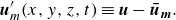 \begin{align} \boldsymbol{u}^\prime _m(x,y,z,t)&\equiv \boldsymbol{u}-\boldsymbol{\bar {u}_m}.\end{align}
We choose the same constant filter width
 $\Delta L=10$
to maximise the time- and duct-volume-averaged kinetic energy. Figure 9(a,b,c) shows the normalised TKE averaged over the duct cross-section and figure 9(d,e,f) shows
$\Delta L=10$
to maximise the time- and duct-volume-averaged kinetic energy. Figure 9(a,b,c) shows the normalised TKE averaged over the duct cross-section and figure 9(d,e,f) shows
 $\widetilde {G}$
. For comparison, we also show the modified composite Froude number for the two-layer hydraulic model,
$\widetilde {G}$
. For comparison, we also show the modified composite Froude number for the two-layer hydraulic model,
 \begin{equation} \widetilde {G}^{2L}=1+\frac {h_1^{2L}+h_2^{2L}}{\big({\rho }_2^{2L}-{\rho }_1^{2L}\big) {Ri} \cos {\theta } \ h_1^{2L} h_2^{2L}} \ \lambda _1^{R^{2L}} \ \lambda _2^{R^{2L}} \end{equation}
in figure 9(g,h,i), where the superscripts ‘2L’ denote variables based on the two-layer averaging of Atoufi et al. (Reference Atoufi, Zhu, Lefauve, Taylor, Kerswell, Dalziel, Lawrence and Linden2023) where the expressions for
 $\lambda _1$
and
$\lambda _1$
and
 $\lambda _2$
are also given in their (4.10).
$\lambda _2$
are also given in their (4.10).
As expected,
 $\widetilde {G}$
in figure 9(e) is consistent with figure 6(a,b) for the TW in the sense that it indicates control points as well as the hydraulic regime. In all three cases, the flow experiences a transition from supercritical to subcritical in the central region of the duct where
$\widetilde {G}$
in figure 9(e) is consistent with figure 6(a,b) for the TW in the sense that it indicates control points as well as the hydraulic regime. In all three cases, the flow experiences a transition from supercritical to subcritical in the central region of the duct where
 $\widetilde {G}$
changes sign. The same auxiliary dashed guidelines (i.e. space–time variation of middle layer height) presented in figures 3 and 6 agree well with
$\widetilde {G}$
changes sign. The same auxiliary dashed guidelines (i.e. space–time variation of middle layer height) presented in figures 3 and 6 agree well with
 $\widetilde {G} \approx 1$
. We observe a similar agreement between
$\widetilde {G} \approx 1$
. We observe a similar agreement between
 $\widetilde {G}$
and the characteristics in the SW and I cases, although their
$\widetilde {G}$
and the characteristics in the SW and I cases, although their
 $x{-}t$
plots are not shown for brevity. Therefore,
$x{-}t$
plots are not shown for brevity. Therefore,
 $\widetilde {G}$
identifies hydraulic regimes and control (i.e. flow regularisation when
$\widetilde {G}$
identifies hydraulic regimes and control (i.e. flow regularisation when
 $G=\tilde {G}=1$
discussed in § 3.4) even in the presence of mixing and beyond the limit where (3.1) is no longer hyperbolic. Although not shown here, the contours of
$G=\tilde {G}=1$
discussed in § 3.4) even in the presence of mixing and beyond the limit where (3.1) is no longer hyperbolic. Although not shown here, the contours of
 $G$
have qualitatively similar patterns to
$G$
have qualitatively similar patterns to
 $\widetilde {G}$
except that
$\widetilde {G}$
except that
 $G \geqslant 1$
in the entire
$G \geqslant 1$
in the entire
 $x{-}t$
plots for the SW, TW and I cases due to
$x{-}t$
plots for the SW, TW and I cases due to
 $\lambda ^I \ne 0$
. Reduced values of
$\lambda ^I \ne 0$
. Reduced values of
 $G$
are also observed at the same locations and times where
$G$
are also observed at the same locations and times where
 $\widetilde {G} \lt 0$
in figure 9(d,e,f).
$\widetilde {G} \lt 0$
in figure 9(d,e,f).
In the centre of the duct between the auxiliary curved lines (corresponding to the upper and lower interface locations) in figure 9, the averaged TKE tends to be elevated in the TW and I cases (figure 9
b,c), suggesting a correlation between enhanced turbulence and hydraulic regime transitions identified by
 $\widetilde {G} = 1$
(figure 9
e,f). In these cases, large values of
$\widetilde {G} = 1$
(figure 9
e,f). In these cases, large values of
 $\langle k_m^{\prime } \rangle _{y,z}$
coincide with regions where
$\langle k_m^{\prime } \rangle _{y,z}$
coincide with regions where
 $\widetilde {G}$
transitions from
$\widetilde {G}$
transitions from
 $\widetilde {G} \gt 1$
(supercritical) to
$\widetilde {G} \gt 1$
(supercritical) to
 $\widetilde {G} \lt 1$
(subcritical), particularly near the duct exits and within central interior regions. In the SW case (figure 9
a) this trend is less apparent where the TKE appears visually weak across most of the space–time domain. This reflects a lower level of turbulence rather than a lack of correlation. Nevertheless, localised turbulence is still present, especially near the duct ends and at the central region, which align with changes in
$\widetilde {G} \lt 1$
(subcritical), particularly near the duct exits and within central interior regions. In the SW case (figure 9
a) this trend is less apparent where the TKE appears visually weak across most of the space–time domain. This reflects a lower level of turbulence rather than a lack of correlation. Nevertheless, localised turbulence is still present, especially near the duct ends and at the central region, which align with changes in
 $\widetilde {G}$
(figure 9
d). These observations indicate that, although the spatiotemporal correspondence between TKE and hydraulic regime transitions is strongest in the TW case and more distributed in the I case, it remains qualitatively evident across all three cases. In the I case, small-scale shear instabilities – such as Kelvin–Helmholtz roll-up and breakdown – embedded within the non-hydrostatic pressure gradient force
$\widetilde {G}$
(figure 9
d). These observations indicate that, although the spatiotemporal correspondence between TKE and hydraulic regime transitions is strongest in the TW case and more distributed in the I case, it remains qualitatively evident across all three cases. In the I case, small-scale shear instabilities – such as Kelvin–Helmholtz roll-up and breakdown – embedded within the non-hydrostatic pressure gradient force
 $\boldsymbol{\mathcal{F}}$
also contribute to turbulence generation, in addition to hydraulic effects that are primarily governed by the hydrostatic pressure distribution. As shown in Atoufi et al. (Reference Atoufi, Zhu, Lefauve, Taylor, Kerswell, Dalziel, Lawrence and Linden2023), the influence of non-hydrostatic pressure is more pronounced in the I case than in the SW and TW cases.
$\boldsymbol{\mathcal{F}}$
also contribute to turbulence generation, in addition to hydraulic effects that are primarily governed by the hydrostatic pressure distribution. As shown in Atoufi et al. (Reference Atoufi, Zhu, Lefauve, Taylor, Kerswell, Dalziel, Lawrence and Linden2023), the influence of non-hydrostatic pressure is more pronounced in the I case than in the SW and TW cases.
Near both ends, we typically observe short waves forming and breaking leading to turbulence (Zhu et al. Reference Zhu, Atoufi, Lefauve, Taylor, Kerswell, Dalziel, Lawrence and Linden2023), suggesting that the flow is unstable to both long- and short-wave instabilities there. As we approach the centre of the duct, the contribution of long waves to the destabilisation of the flow becomes increasingly significant.
For the two-layer model,
 $\widetilde {G}^{2L} = 1$
is more weakly correlated with
$\widetilde {G}^{2L} = 1$
is more weakly correlated with
 $\langle k^\prime _m\rangle _{y,z}$
. A key result of this paper is that the three-layer
$\langle k^\prime _m\rangle _{y,z}$
. A key result of this paper is that the three-layer
 $\widetilde {G}$
outperforms the two-layer
$\widetilde {G}$
outperforms the two-layer
 $\widetilde {G}^{2L}$
in predicting regions (not only points) where the flow is most unstable and turbulent. Therefore, regime transitions identified by changes in sign of
$\widetilde {G}^{2L}$
in predicting regions (not only points) where the flow is most unstable and turbulent. Therefore, regime transitions identified by changes in sign of
 $\widetilde {G}$
(i.e. changes in the direction of information propagation) provide excellent predictions of where and when turbulence is generated and strong mixing is expected in stratified exchange flows. The mechanism underlying this agreement is explained in § 4.
$\widetilde {G}$
(i.e. changes in the direction of information propagation) provide excellent predictions of where and when turbulence is generated and strong mixing is expected in stratified exchange flows. The mechanism underlying this agreement is explained in § 4.
3.4. Hydraulic control mechanisms
The characteristics specify the directions of information propagation whereas the control mechanisms specify how information propagates along the characteristics (see § 3.2). Hydraulic control mechanisms are set by some regularity conditions where hydraulic regime transitions occur. To see this link, one can deduce from (3.19) that a solution exists either when
 ${\det}\; \unicode{x1D63C}\ne 0$
or when
${\det}\; \unicode{x1D63C}\ne 0$
or when
 ${\det}\; \unicode{x1D63C}=0$
with some regularity conditions allowing acceptable solutions. Mathematically, at the control points where
${\det}\; \unicode{x1D63C}=0$
with some regularity conditions allowing acceptable solutions. Mathematically, at the control points where
 ${\det}\; \unicode{x1D63C}=0$
the flow should be regularised by the condition
${\det}\; \unicode{x1D63C}=0$
the flow should be regularised by the condition
 \begin{equation} {\bigg\lVert {{\rm adj} (\unicode{x1D63C}) \unicode{x1D63D}\frac {\partial \boldsymbol{s}}{\partial x}} \bigg\rVert }{_F}=0 \ \ {(\textrm{inviscid})}\quad {\text{and}} \quad {\lVert {{\rm adj} (\unicode{x1D63C}) {\tau } \boldsymbol{q}} \rVert }{_F}=\boldsymbol{0} \ \ {(\textrm{viscous})}, \end{equation}
where
 ${\lVert {\cdot } \rVert }_F$
refers to the Frobenius norm.
${\lVert {\cdot } \rVert }_F$
refers to the Frobenius norm.
3.4.1. Inviscid control mechanism
The inviscid regularity condition in (3.29) implies that
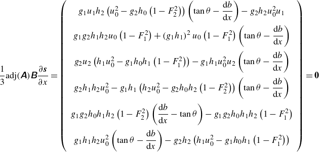 \begin{align} \frac {1}{3} {\rm adj} (\unicode{x1D63C}) \unicode{x1D63D}\frac {\partial \boldsymbol{s}}{\partial x}= \left (\begin{array}{c} g_1 u_1 h_2 \left ( {u_0^2 } - g_2 h_0 \left (1-F_2^2 \right )\right ) \left (\tan {\theta }-\dfrac {\text{d} b}{\text{d} x} \right ) -g_2 h_2 {u_0^2 } u_1 \\[10pt] g_1 g_2 h_1 h_2 u_0 \left (1-F_1^2\right ) +\left (g_1 h_1\right )^2 u_0 \left (1-F_1^2\right ) \left (\tan {\theta } -\dfrac {\text{d} b}{\text{d} x} \right )\\[12pt] g_2 u_2 \left (h_1 {u_0^2 } - g_1 h_0 h_1 \left (1-F_1^2\right )\right ) -g_1 h_1 {u_0^2 } u_2 \left (\tan {\theta }-\dfrac {\text{d} b}{\text{d} x}\right ) \\[12pt] g_2 h_1 h_2 {u_0^2 } -g_1 h_1 \left (h_2 {u_0^2 } - g_2 h_0 h_2 \left (1-F_2^2 \right )\right ) \left (\tan {\theta } -\dfrac {\text{d} b}{\text{d} x} \right ) \\[12pt] g_1 g_2 h_0 h_1 h_2 \left (1-F_2^2 \right ) \left (\dfrac {\text{d} b}{\text{d} x}-\tan {\theta } \right ) -g_1 g_2 h_0 h_1 h_2 \left (1-F_1^2\right ) \\[12pt] g_1 h_1 h_2 {u_0^2 } \left (\tan {\theta }-\dfrac {\text{d} b}{\text{d} x} \right )-g_2 h_2 \left (h_1 {u_0^2 } - g_1 h_0 h_1 \left (1-F_1^2\right )\right ) \end{array}\right )=\boldsymbol{0} \end{align}
at the control points. We recall that two conditions lead to
 ${\det}\; \unicode{x1D63C}=0$
and hydraulic control: either (i)
${\det}\; \unicode{x1D63C}=0$
and hydraulic control: either (i)
 $h_0=0$
or (ii)
$h_0=0$
or (ii)
 $h_0 \neq 0$
but
$h_0 \neq 0$
but
 $G=1$
, which further requires
$G=1$
, which further requires
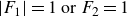 ${\lvert {F_1 } \rvert }=1 \ \text{or} \ {F_2 }=1$
and
${\lvert {F_1 } \rvert }=1 \ \text{or} \ {F_2 }=1$
and
 $F_0=0$
(i.e.
$F_0=0$
(i.e.
 $u_0=0$
).
$u_0=0$
).
For condition (i), (3.30) enforces
 $u_0=0$
. Therefore, both the criticality and inviscid control mechanisms imply that the middle layer velocity vanishes near the jumps. This is consistent with the sudden reduction of
$u_0=0$
. Therefore, both the criticality and inviscid control mechanisms imply that the middle layer velocity vanishes near the jumps. This is consistent with the sudden reduction of
 $\lvert {u_0} \rvert$
near the duct ends and close to the control point in figure 4(d). Note that near the duct ends where
$\lvert {u_0} \rvert$
near the duct ends and close to the control point in figure 4(d). Note that near the duct ends where
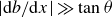 ${\lvert {{\text{d} b}/{\text{d} x}} \rvert } \gg \tan {\theta }$
the flow is also hydraulically controlled as
${\lvert {{\text{d} b}/{\text{d} x}} \rvert } \gg \tan {\theta }$
the flow is also hydraulically controlled as
 $h_0 \approx 0$
(condition (i)) and
$h_0 \approx 0$
(condition (i)) and
 $\lvert {u_0} \rvert$
drops sharply in figure 4(a) to satisfy (3.30). Inside the duct
$\lvert {u_0} \rvert$
drops sharply in figure 4(a) to satisfy (3.30). Inside the duct
 ${\text{d} b}/{\text{d} x}=0$
and
${\text{d} b}/{\text{d} x}=0$
and
 $\lvert {u_0} \rvert$
drops more smoothly.
$\lvert {u_0} \rvert$
drops more smoothly.
As stated above, one possibility for
 $G=1$
is
$G=1$
is
 $F_0=0$
and either
$F_0=0$
and either
 ${\lvert {F_1} \rvert }=1$
or
${\lvert {F_1} \rvert }=1$
or
 ${\lvert {F_2} \rvert }=1$
at control points. For condition (ii), (3.30) enforces that
${\lvert {F_2} \rvert }=1$
at control points. For condition (ii), (3.30) enforces that
 ${\lvert {F_1} \rvert }=1$
(critical upper layer) yields
${\lvert {F_1} \rvert }=1$
(critical upper layer) yields
 ${\lvert {F_2} \rvert }=1$
(critical lower layer), assuming the middle layer has non-zero velocity. However, this implication does not hold in general. For example, when
${\lvert {F_2} \rvert }=1$
(critical lower layer), assuming the middle layer has non-zero velocity. However, this implication does not hold in general. For example, when
 $u_0 = 0$
,
$u_0 = 0$
,
 $F_1 = 0$
and
$F_1 = 0$
and
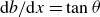 ${\text{d} b}/{\text{d} x} = \tan \theta$
, all terms in (3.30) vanish, the condition is trivially satisfied and does not constrain
${\text{d} b}/{\text{d} x} = \tan \theta$
, all terms in (3.30) vanish, the condition is trivially satisfied and does not constrain
 $F_2$
, meaning that both interfaces need not be simultaneously critical. This reflects the fact that when the middle layer is stationary near the control point, the system may exhibit decoupled dynamics at the upper and lower interfaces. Criticality may occur in one interface without enforcing it in the other as also discussed for the special case of pure exchange flow in § 3.2.2. This type of decoupling, particularly relevant for
$F_2$
, meaning that both interfaces need not be simultaneously critical. This reflects the fact that when the middle layer is stationary near the control point, the system may exhibit decoupled dynamics at the upper and lower interfaces. Criticality may occur in one interface without enforcing it in the other as also discussed for the special case of pure exchange flow in § 3.2.2. This type of decoupling, particularly relevant for
 $ N$
-layer (
$ N$
-layer (
 $N\gt 2$
) flows with stagnant interior layers, was analysed by Engqvist (Reference Engqvist1996), who showed that under such conditions, the upper and lower groups of non-stagnant layers can be governed by independent control criteria.
$N\gt 2$
) flows with stagnant interior layers, was analysed by Engqvist (Reference Engqvist1996), who showed that under such conditions, the upper and lower groups of non-stagnant layers can be governed by independent control criteria.
In summary, in addition to flow regularisation, condition (i) implies a thin middle layer and a two-layer exchange flow at both ends. Under condition (ii), when the middle layer is dynamically active, the two oppositely propagating flows at critical velocity (
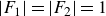 ${\lvert {F_1} \rvert } = {\lvert {F_2} \rvert } = 1$
) cause vigorous mixing (
${\lvert {F_1} \rvert } = {\lvert {F_2} \rvert } = 1$
) cause vigorous mixing (
 $h_0 \ne 0$
) in the middle of the duct (due to symmetry). However, when the middle layer is stationary near the control, the upper and lower interfaces may become decoupled, and criticality may occur independently at one or both interfaces without requiring symmetry.
$h_0 \ne 0$
) in the middle of the duct (due to symmetry). However, when the middle layer is stationary near the control, the upper and lower interfaces may become decoupled, and criticality may occur independently at one or both interfaces without requiring symmetry.
3.4.2. Viscous control mechanism
The effects of viscosity are of particular importance as they allow for enhanced dissipation in hydraulic jumps, and are connected to turbulent mixing when the hydraulic regime transitions from supercritical to subcritical.
In figure 10 we computed the viscous control term
 ${\tau } \boldsymbol{q}$
(non-zero elements) to verify that it indeed dominates the right-hand side of (3.1) in the central region of the duct where
${\tau } \boldsymbol{q}$
(non-zero elements) to verify that it indeed dominates the right-hand side of (3.1) in the central region of the duct where
 $\widetilde {G} = 1$
(at a representative time
$\widetilde {G} = 1$
(at a representative time
 $t=110$
). Panels (a,b) present the viscous terms and the sum of all the terms on the right of (3.1), respectively, and show that the viscous term dominates, particularly in the central region of the duct. For the wave cases, the viscous control mechanism, represented by
$t=110$
). Panels (a,b) present the viscous terms and the sum of all the terms on the right of (3.1), respectively, and show that the viscous term dominates, particularly in the central region of the duct. For the wave cases, the viscous control mechanism, represented by
 $\boldsymbol{\tau q}$
, becomes
$\boldsymbol{\tau q}$
, becomes
 $\lesssim 0.01$
in the centre of the duct to regulate the flow (§ 3.4) at the internal control points. The summation of these terms also reaches a local minimum near the control points. Note that the viscous term and sum also become approximately zero at the duct ends, where geometric control is established. The regularity condition is therefore satisfied for all control mechanisms at the duct ends.
$\lesssim 0.01$
in the centre of the duct to regulate the flow (§ 3.4) at the internal control points. The summation of these terms also reaches a local minimum near the control points. Note that the viscous term and sum also become approximately zero at the duct ends, where geometric control is established. The regularity condition is therefore satisfied for all control mechanisms at the duct ends.
The large contribution of viscous terms
 ${\tau } \boldsymbol{q}$
suggests that information propagation along the interfaces is predominantly modulated by viscous effects (see § 3.2). By comparing figures 7 and 10, we observe that along the upper interface, viscous damping occurs on the left side of the duct, where
${\tau } \boldsymbol{q}$
suggests that information propagation along the interfaces is predominantly modulated by viscous effects (see § 3.2). By comparing figures 7 and 10, we observe that along the upper interface, viscous damping occurs on the left side of the duct, where
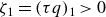 $\zeta _1 = (\tau q)_1 \gt 0$
(with the subscript 1 indicating the term from the velocity difference equation between the middle and upper layers, i.e. the first row of (3.1)) and
$\zeta _1 = (\tau q)_1 \gt 0$
(with the subscript 1 indicating the term from the velocity difference equation between the middle and upper layers, i.e. the first row of (3.1)) and
 $\lambda _1^R \gt 0$
, indicating viscous dissipation. On the right side of the duct, where
$\lambda _1^R \gt 0$
, indicating viscous dissipation. On the right side of the duct, where
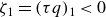 $\zeta _1 = (\tau q)_1 \lt 0$
and
$\zeta _1 = (\tau q)_1 \lt 0$
and
 $\lambda _1^R \lt 0$
, the viscous forcing reinforces the direction of wave propagation. This results in a local amplification of interfacial waves due to enhanced mixing with the lower layer. Similarly, along the lower interface, viscous damping is observed on the right side, where
$\lambda _1^R \lt 0$
, the viscous forcing reinforces the direction of wave propagation. This results in a local amplification of interfacial waves due to enhanced mixing with the lower layer. Similarly, along the lower interface, viscous damping is observed on the right side, where
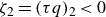 $\zeta _2 = (\tau q)_2 \lt 0$
and
$\zeta _2 = (\tau q)_2 \lt 0$
and
 $\lambda _3^R \gt 0$
, again indicating dissipation. Here, the subscript 2 refers to the velocity difference equation between the lower and middle layers (the second row of (3.1)). On the left side, where
$\lambda _3^R \gt 0$
, again indicating dissipation. Here, the subscript 2 refers to the velocity difference equation between the lower and middle layers (the second row of (3.1)). On the left side, where
 $(\tau q)_2 \gt 0$
and
$(\tau q)_2 \gt 0$
and
 $\lambda _3^R \lt 0$
, viscous forcing contributes constructively to wave propagation, leading to amplification through mixing with the upper layer.
$\lambda _3^R \lt 0$
, viscous forcing contributes constructively to wave propagation, leading to amplification through mixing with the upper layer.
Control mechanisms that dictate how information propagates along the characteristics in the three-layer model at
 $t = 110$
for all cases: (a) viscous control and (b) the sum of all terms on the right-hand side of (3.1). Solid lines (
$t = 110$
for all cases: (a) viscous control and (b) the sum of all terms on the right-hand side of (3.1). Solid lines (
 $\zeta _1$
) and dashed lines (
$\zeta _1$
) and dashed lines (
 $\zeta _2$
) represent the first and second momentum equations (first and second rows, respectively) in (3.1). The lines are shown for the SW, TW and I cases in light purple, dark purple and yellow, respectively.
$\zeta _2$
) represent the first and second momentum equations (first and second rows, respectively) in (3.1). The lines are shown for the SW, TW and I cases in light purple, dark purple and yellow, respectively.
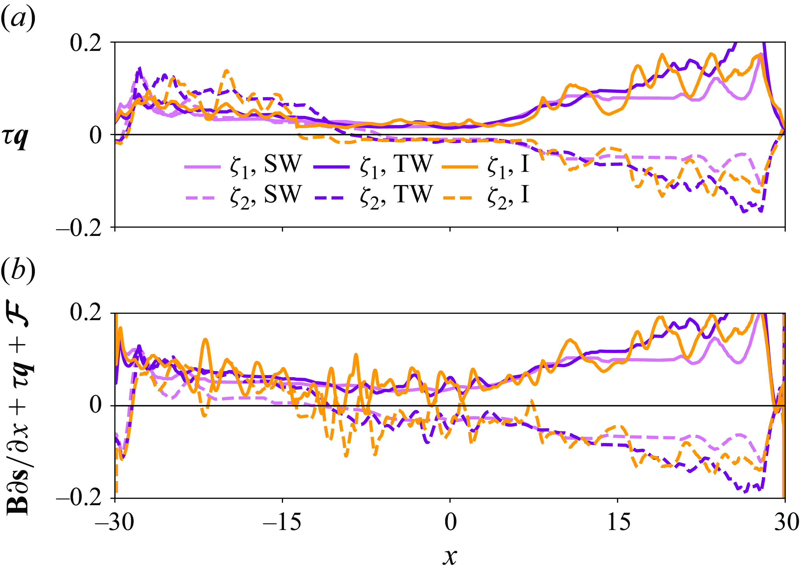
Thus far our focus has been primarily on the physical significance of characteristics in hydraulic control and regime transition embedded in
 $\lambda ^R$
. Although we showed a strong correlation between turbulence generation and
$\lambda ^R$
. Although we showed a strong correlation between turbulence generation and
 $\lambda ^R$
, to reveal their true connections, we need to consider instabilities through the imaginary part
$\lambda ^R$
, to reveal their true connections, we need to consider instabilities through the imaginary part
 $\lambda ^I$
, as we do next.
$\lambda ^I$
, as we do next.
Space–time plots of the long-wave growth rate simultaneity,
 $\lambda _2^I \lambda _4^I$
, for (a) SW, (b) TW and (c) I cases.
$\lambda _2^I \lambda _4^I$
, for (a) SW, (b) TW and (c) I cases.
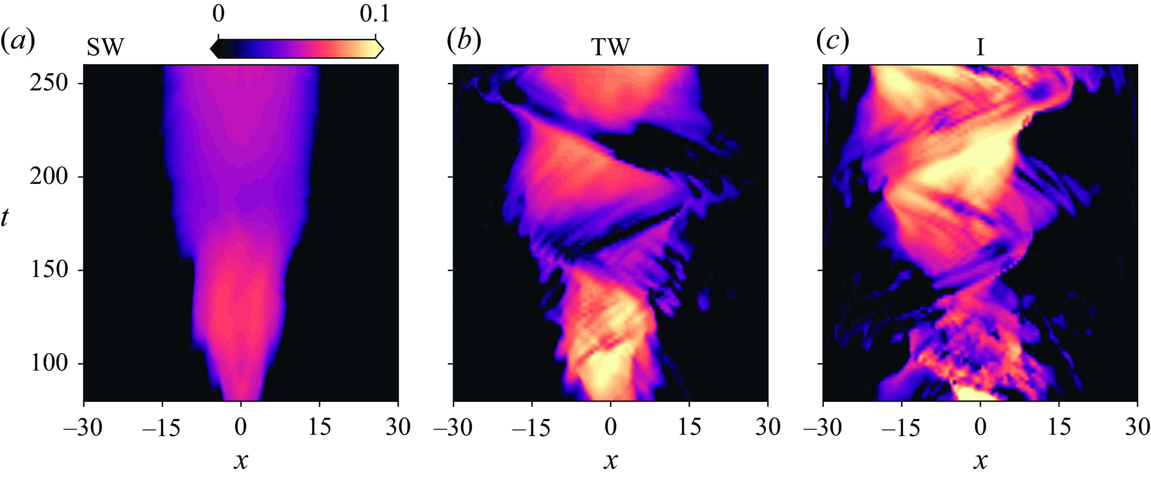
4. Three-layer instabilities and resonances
4.1. Simultaneous amplification in the growth rate of the long waves
In Appendix A we show that the characteristics
 $\lambda$
obtained from (3.9) are identical to the phase speed of linear long waves (with wavenumber
$\lambda$
obtained from (3.9) are identical to the phase speed of linear long waves (with wavenumber
 $k\ll 1$
) propagating in a background three-layer flow. In § 3 we discussed the essential roles of the
$k\ll 1$
) propagating in a background three-layer flow. In § 3 we discussed the essential roles of the
 $\lambda ^R$
to predict the control points and hydraulic regimes, which are closely associated with the laminar–turbulence transition in SID flows. Nonetheless, a consequence of the equality of the
$\lambda ^R$
to predict the control points and hydraulic regimes, which are closely associated with the laminar–turbulence transition in SID flows. Nonetheless, a consequence of the equality of the
 $\lambda$
and phase velocity of the linear long wave is that
$\lambda$
and phase velocity of the linear long wave is that
 $\lambda ^I\gt 0$
represents their growth rate. Therefore, it is reasonable to anticipate that the space–time distribution of the imaginary components presented in figure 6(c,d) may be a proxy to the TKE shown in figure 9(a,b,c). However, upon comparing their distributions, it is evident that this is not the case. In figure 6(c) the imaginary components of characteristics of the upper interface
$\lambda ^I\gt 0$
represents their growth rate. Therefore, it is reasonable to anticipate that the space–time distribution of the imaginary components presented in figure 6(c,d) may be a proxy to the TKE shown in figure 9(a,b,c). However, upon comparing their distributions, it is evident that this is not the case. In figure 6(c) the imaginary components of characteristics of the upper interface
 $\lambda _1^I$
exhibit a positive growth rate in the right and middle regions of the duct (separated by the auxiliary lines in figure 6
c), while
$\lambda _1^I$
exhibit a positive growth rate in the right and middle regions of the duct (separated by the auxiliary lines in figure 6
c), while
 $\lambda _3^I$
associated with the lower interface displays a positive imaginary component in the middle and right regions of the duct. They do not match with the TKE distribution in figure 9(b), which shows the largest TKE in the middle of the duct. However, when multiplying
$\lambda _3^I$
associated with the lower interface displays a positive imaginary component in the middle and right regions of the duct. They do not match with the TKE distribution in figure 9(b), which shows the largest TKE in the middle of the duct. However, when multiplying
 $\lambda _2^I(x,t)$
and
$\lambda _2^I(x,t)$
and
 $\lambda _4^I(x,t)$
to diagnose whether both interfaces simultaneously grow or not, we expect
$\lambda _4^I(x,t)$
to diagnose whether both interfaces simultaneously grow or not, we expect
 $\lambda _2^I\lambda _4^I(x,t)$
to agree with the TKE distribution, which will be discussed next.
$\lambda _2^I\lambda _4^I(x,t)$
to agree with the TKE distribution, which will be discussed next.
We show in figure 11 the spatiotemporal distribution of the simultaneous amplification
 $\lambda _2^I \lambda _4^I(x,t)$
, reflecting the growth of long waves at the upper and lower interfaces in the SW (a), TW (b) and I (c) regimes. In all cases, the central region of the duct exhibits the largest
$\lambda _2^I \lambda _4^I(x,t)$
, reflecting the growth of long waves at the upper and lower interfaces in the SW (a), TW (b) and I (c) regimes. In all cases, the central region of the duct exhibits the largest
 $\lambda _2^I \lambda _4^I$
and the amplitude growth of the long waves (indicated by light colours) occurs at the same rate, even though
$\lambda _2^I \lambda _4^I$
and the amplitude growth of the long waves (indicated by light colours) occurs at the same rate, even though
 $\lambda _2^I$
and
$\lambda _2^I$
and
 $\lambda _4^I$
attain their highest values in regions corresponding to dark contours. A qualitative correspondence can be observed between regions of elevated
$\lambda _4^I$
attain their highest values in regions corresponding to dark contours. A qualitative correspondence can be observed between regions of elevated
 $\lambda _2^I \lambda _4^I$
in figure 11 and enhanced TKE in figure 9(a–c), particularly in the TW and I cases. In these cases, simultaneous growth in the amplitude of long interfacial waves is followed (with some time delay) by the emergence of turbulence, supporting a linkage between long-wave amplification and the eventual onset of smaller-scale generation through nonlinear energy transfer and wave breaking. In the SW case, however, this correspondence is less clear due to weaker turbulence levels. Differences across the cases may also arise from the emergence of short-wave instabilities, which are addressed in the following section.
$\lambda _2^I \lambda _4^I$
in figure 11 and enhanced TKE in figure 9(a–c), particularly in the TW and I cases. In these cases, simultaneous growth in the amplitude of long interfacial waves is followed (with some time delay) by the emergence of turbulence, supporting a linkage between long-wave amplification and the eventual onset of smaller-scale generation through nonlinear energy transfer and wave breaking. In the SW case, however, this correspondence is less clear due to weaker turbulence levels. Differences across the cases may also arise from the emergence of short-wave instabilities, which are addressed in the following section.
Further understanding of the simultaneous growth in a three-layer exchange flow can be gained by building-block decomposition of the inviscid homogeneous limit of (3.1), which will be discussed next.
4.2. Instability arising from long waves: isolated-layer perturbation
Although
 $\lambda ^I$
represents the growth rate of the linear long waves (see Appendix A), the origin of this imaginary component in the characteristics remains unclear. In two-layer flows the presence of
$\lambda ^I$
represents the growth rate of the linear long waves (see Appendix A), the origin of this imaginary component in the characteristics remains unclear. In two-layer flows the presence of
 $\lambda ^I$
is linked to the cross-interface shear exceeding a certain threshold, which induces the appearance of the imaginary component (Long Reference Long1956; Dalziel Reference Dalziel1991; Lawrence Reference Lawrence1993; Atoufi et al. Reference Atoufi, Zhu, Lefauve, Taylor, Kerswell, Dalziel, Lawrence and Linden2023). However, for three-layer flows, identifying a single threshold is not feasible due to the increased complexity and number of variables involved. The resulting analytical expression for the characteristics, as given in (3.12), is too lengthy and intricate to define a simple criterion. Therefore, we seek an alternative approach that relates
$\lambda ^I$
is linked to the cross-interface shear exceeding a certain threshold, which induces the appearance of the imaginary component (Long Reference Long1956; Dalziel Reference Dalziel1991; Lawrence Reference Lawrence1993; Atoufi et al. Reference Atoufi, Zhu, Lefauve, Taylor, Kerswell, Dalziel, Lawrence and Linden2023). However, for three-layer flows, identifying a single threshold is not feasible due to the increased complexity and number of variables involved. The resulting analytical expression for the characteristics, as given in (3.12), is too lengthy and intricate to define a simple criterion. Therefore, we seek an alternative approach that relates
 $\lambda ^I$
to interactions between the layers.
$\lambda ^I$
to interactions between the layers.
We focus on the free propagation of the long waves described by the inviscid homogeneous limit of (3.1) where
 $\unicode{x1D63E}({\partial \boldsymbol{q}}/{\partial t})+\unicode{x1D63C}({\partial \boldsymbol{q}}/{\partial x})=\boldsymbol{0}$
and we decompose the coefficient matrices as
$\unicode{x1D63E}({\partial \boldsymbol{q}}/{\partial t})+\unicode{x1D63C}({\partial \boldsymbol{q}}/{\partial x})=\boldsymbol{0}$
and we decompose the coefficient matrices as
 \begin{equation} \begin{aligned} \unicode{x1D63C}=\bigg(\unicode{x1D63C}_1+\frac {\unicode{x1D63C}_0}{2}\bigg)+\bigg(\unicode{x1D63C}_2+\frac {\unicode{x1D63C}_0}{2}\bigg), \\ \nonumber \unicode{x1D63E}=\bigg(\unicode{x1D63E}_1+\frac {\unicode{x1D63E}_0}{2}\bigg)+\bigg(\unicode{x1D63E}_2+\frac {\unicode{x1D63E}_0}{2}\bigg),\end{aligned} \end{equation}
such that
 \begin{align} \unicode{x1D63C}_i &= \left (\begin{array}{cccccc} -u_1 \delta _{i1} & u_0 \delta _{i0} & 0 & 0 & g_1 & g_1\\ 0 & -u_0 \delta _{i0} & u_2 \delta _{i2} & 0 & 0 & g_2 \\ -h_1 & h_0 & 0 & -u_1 \delta _{i1} & u_0 \delta _{i0} & 0\\ 0 & -h_0 & h_2 & 0 & -u_0 \delta _{i0} & u_2 \delta _{i2} \\ 0 & 0 & 0 & 1 & 1 & 1\\ h_1 & h_0 & h_2 & u_1 \delta _{i1} & u_0 \delta _{i0} & u_2 \delta _{i2} \end{array}\right ), \end{align}
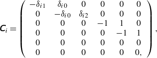 \begin{eqnarray} \unicode{x1D63E}_i & = & \left (\begin{array}{cccccc} -\delta _{i1} & \delta _{i0} & 0 & 0 & 0 & 0\\ 0 & -\delta _{i0} & \delta _{i2} & 0 & 0 & 0 \\ 0 & 0 & 0 & -1 & 1 & 0\\ 0 & 0 & 0 & 0 & -1 & 1 \\ 0 & 0 & 0 & 0 & 0 & 0\\ 0 & 0 & 0 & 0 & 0 & 0, \end{array}\right ), \end{eqnarray}
where
 $i=0,1,2$
and
$i=0,1,2$
and
 $\delta _{ij}$
denotes the Kronecker delta function. To facilitate theory, we introduce the coefficient matrix pairs
$\delta _{ij}$
denotes the Kronecker delta function. To facilitate theory, we introduce the coefficient matrix pairs
 \begin{eqnarray} \unicode{x1D652}=(\unicode{x1D63C}_1,\unicode{x1D63E}_1), \quad \unicode{x1D654}=(\unicode{x1D63C}_2,\unicode{x1D63E}_2), \quad \unicode{x1D655}=({\unicode{x1D63C}_0},{\unicode{x1D63E}_0}{\kern2pt}). \end{eqnarray}
The first matrix pair,
 $\unicode{x1D652}$
, represents an isolated upper layer moving over stationary middle and lower layers, as if these two layers act as a hypothetical topography that restricts the frictionless motion of the upper layer. Notably,
$\unicode{x1D652}$
, represents an isolated upper layer moving over stationary middle and lower layers, as if these two layers act as a hypothetical topography that restricts the frictionless motion of the upper layer. Notably,
 $u_0$
and
$u_0$
and
 $u_2$
from
$u_2$
from
 $\unicode{x1D63C}$
and the corresponding columns in
$\unicode{x1D63C}$
and the corresponding columns in
 $\unicode{x1D63E}$
do not appear in
$\unicode{x1D63E}$
do not appear in
 $\unicode{x1D652}$
, reflecting the isolation of the upper layer. Similarly, the second matrix pair,
$\unicode{x1D652}$
, reflecting the isolation of the upper layer. Similarly, the second matrix pair,
 $\unicode{x1D654}$
, denotes the isolated lower layer moving without friction beneath the stationary middle and upper layers, which act as a topography restricting its motion. Here,
$\unicode{x1D654}$
, denotes the isolated lower layer moving without friction beneath the stationary middle and upper layers, which act as a topography restricting its motion. Here,
 $u_0$
and
$u_0$
and
 $u_1$
from
$u_1$
from
 $\unicode{x1D63C}$
and their corresponding columns in
$\unicode{x1D63C}$
and their corresponding columns in
 $\unicode{x1D63E}$
are absent from
$\unicode{x1D63E}$
are absent from
 $\unicode{x1D654}$
. Finally, the third matrix pair,
$\unicode{x1D654}$
. Finally, the third matrix pair,
 $\unicode{x1D655}$
, represents an isolated middle layer moving without friction between the ‘topography’ provided by the stationary upper and lower layers.
$\unicode{x1D655}$
, represents an isolated middle layer moving without friction between the ‘topography’ provided by the stationary upper and lower layers.
The generalised eigenvalue problem associated with each matrix pair has only real solutions of the form:
 \begin{align} \lambda (\unicode{x1D652}{\kern2pt}) & = u_1 \pm \sqrt {g_1 h_1},\end{align}
 \begin{align} \lambda (\unicode{x1D655}{\kern2.5pt})& = \left (u_0 - \sqrt {\frac {g_1 g_2}{g_1+g_2} h_0}\right )\left (u_0 + \sqrt {\frac {g_1 g_2}{g_1+g_2} h_0}\right ),\end{align}
 \begin{align} \lambda (\unicode{x1D654}{\kern2.5pt})& = u_2 \pm \sqrt {g_2 h_2}.\end{align}
Now consider that the isolated upper layer matrix pair
 $\unicode{x1D652}$
is perturbed by
$\unicode{x1D652}$
is perturbed by
 $\unicode{x1D655}/2$
through the interaction between the upper and middle layers. Similarly, we allow
$\unicode{x1D655}/2$
through the interaction between the upper and middle layers. Similarly, we allow
 $\unicode{x1D655}/2$
to perturb the isolated lower layer, accounting for the interaction between the lower and middle layers. We denote these perturbed layers with the following matrix pairs:
$\unicode{x1D655}/2$
to perturb the isolated lower layer, accounting for the interaction between the lower and middle layers. We denote these perturbed layers with the following matrix pairs:
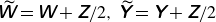 $\,\widetilde {\!{\kern-1pt}\unicode{x1D652}} = \unicode{x1D652} + \unicode{x1D655}/2, \ \,\widetilde {\!{\kern-1pt}\unicode{x1D654}} = \unicode{x1D654} + \unicode{x1D655}/2$
, and we note that
$\,\widetilde {\!{\kern-1pt}\unicode{x1D652}} = \unicode{x1D652} + \unicode{x1D655}/2, \ \,\widetilde {\!{\kern-1pt}\unicode{x1D654}} = \unicode{x1D654} + \unicode{x1D655}/2$
, and we note that
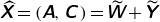 $\,\widehat {\!{\kern-1pt}\unicode{x1D653}} = (\unicode{x1D63C}, \unicode{x1D63E}{\kern2pt}) = \,\widetilde {\!{\kern-1pt}\unicode{x1D652}} + \,\widetilde {\!{\kern-1pt}\unicode{x1D654}}$
. We refer to
$\,\widehat {\!{\kern-1pt}\unicode{x1D653}} = (\unicode{x1D63C}, \unicode{x1D63E}{\kern2pt}) = \,\widetilde {\!{\kern-1pt}\unicode{x1D652}} + \,\widetilde {\!{\kern-1pt}\unicode{x1D654}}$
. We refer to
 $\,\widetilde {\!{\kern-1pt}\unicode{x1D652}}$
as the perturbed upper layer matrix pair and
$\,\widetilde {\!{\kern-1pt}\unicode{x1D652}}$
as the perturbed upper layer matrix pair and
 $\,\widetilde {\!{\kern-1pt}\unicode{x1D654}}$
as the perturbed lower layer matrix pair, noting that
$\,\widetilde {\!{\kern-1pt}\unicode{x1D654}}$
as the perturbed lower layer matrix pair, noting that
 $\,\widehat {\!{\kern-1pt}\unicode{x1D653}}$
yields the original three-layer exchange flow in the inviscid homogeneous limit.
$\,\widehat {\!{\kern-1pt}\unicode{x1D653}}$
yields the original three-layer exchange flow in the inviscid homogeneous limit.
Since the flow is stably stratified, with
 $g_1, g_2 \gt 0$
, all eigenvalues in (4.5) are real. However, the perturbed matrix pairs introduce imaginary components in their characteristics, such that
$g_1, g_2 \gt 0$
, all eigenvalues in (4.5) are real. However, the perturbed matrix pairs introduce imaginary components in their characteristics, such that
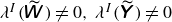 $ \lambda ^I(\,\widetilde {\!{\kern-1pt}\unicode{x1D652}}{\kern2pt}) \neq 0, \ \lambda ^I(\,\widetilde {\!{\kern-1pt}\unicode{x1D654}}{\kern2pt}) \neq 0$
in general. Therefore, attributing the criterion
$ \lambda ^I(\,\widetilde {\!{\kern-1pt}\unicode{x1D652}}{\kern2pt}) \neq 0, \ \lambda ^I(\,\widetilde {\!{\kern-1pt}\unicode{x1D654}}{\kern2pt}) \neq 0$
in general. Therefore, attributing the criterion
 $\lambda ^I(\,\widehat {\!{\kern-1pt}\unicode{x1D653}}{\kern2pt}) \gt 0$
to the onset of long-wave instabilities (see Appendix A) reveals that the instability arises exclusively from
$\lambda ^I(\,\widehat {\!{\kern-1pt}\unicode{x1D653}}{\kern2pt}) \gt 0$
to the onset of long-wave instabilities (see Appendix A) reveals that the instability arises exclusively from
 $\,\widetilde {\!{\kern-1pt}\unicode{x1D652}}$
and
$\,\widetilde {\!{\kern-1pt}\unicode{x1D652}}$
and
 $\,\widetilde {\!{\kern-1pt}\unicode{x1D654}}$
, the perturbed upper and lower isolated layers influenced by the middle layer. We note that
$\,\widetilde {\!{\kern-1pt}\unicode{x1D654}}$
, the perturbed upper and lower isolated layers influenced by the middle layer. We note that
 $\lambda (\unicode{x1D652}+\unicode{x1D654}{\kern2pt}) \in \mathbb{R}$
meaning that perturbing
$\lambda (\unicode{x1D652}+\unicode{x1D654}{\kern2pt}) \in \mathbb{R}$
meaning that perturbing
 $\unicode{x1D652}$
by
$\unicode{x1D652}$
by
 $\unicode{x1D654}$
alone (and vice versa) does not introduce imaginary components in the characteristics. This implies that the origin of the imaginary components results specifically from the interaction of the isolated upper and lower layers with the middle layer.
$\unicode{x1D654}$
alone (and vice versa) does not introduce imaginary components in the characteristics. This implies that the origin of the imaginary components results specifically from the interaction of the isolated upper and lower layers with the middle layer.
The matrix pairs
 $\,\widetilde {\!{\kern-1pt}\unicode{x1D652}}$
and
$\,\widetilde {\!{\kern-1pt}\unicode{x1D652}}$
and
 $\,\widetilde {\!{\kern-1pt}\unicode{x1D654}}$
represent a building-block decomposition, illustrating that the full system
$\,\widetilde {\!{\kern-1pt}\unicode{x1D654}}$
represent a building-block decomposition, illustrating that the full system
 $\,\widehat {\!{\kern-1pt}\unicode{x1D653}}$
comprises two interacting subsystems: the perturbed upper layer (
$\,\widehat {\!{\kern-1pt}\unicode{x1D653}}$
comprises two interacting subsystems: the perturbed upper layer (
 $\,\widetilde {\!{\kern-1pt}\unicode{x1D652}}{\kern2pt}$
) and the perturbed lower layer (
$\,\widetilde {\!{\kern-1pt}\unicode{x1D652}}{\kern2pt}$
) and the perturbed lower layer (
 $\,\widetilde {\!{\kern-1pt}\unicode{x1D654}}{\kern2pt}$
).
$\,\widetilde {\!{\kern-1pt}\unicode{x1D654}}{\kern2pt}$
).
In a three-layer system, three types of resonance are possible: (i) resonance between interfacial waves at the upper interface alone, (ii) resonance at the lower interface alone and (iii) resonance due to interactions between waves propagating on both interfaces. The decomposition into
 $\,\widetilde {\!{\kern-1pt}\unicode{x1D652}}$
and
$\,\widetilde {\!{\kern-1pt}\unicode{x1D652}}$
and
 $\,\widetilde {\!{\kern-1pt}\unicode{x1D654}}$
also offers a framework for diagnosing all three cases by isolating contributions from each layer and their coupling.
$\,\widetilde {\!{\kern-1pt}\unicode{x1D654}}$
also offers a framework for diagnosing all three cases by isolating contributions from each layer and their coupling.
To illustrate this, we consider the special case of pure exchange flow discussed in § 3.2.2. In this case,
 ${\lVert {\,\widetilde {\!{\kern-1pt}\unicode{x1D652}}}\rVert }_F = {\lVert {\,\widetilde {\!{\kern-1pt}\unicode{x1D654}}} \rVert }_F$
, leading to
${\lVert {\,\widetilde {\!{\kern-1pt}\unicode{x1D652}}}\rVert }_F = {\lVert {\,\widetilde {\!{\kern-1pt}\unicode{x1D654}}} \rVert }_F$
, leading to
 $\lambda _{1,2} = \lambda (\,\widetilde {\!{\kern-1pt}\unicode{x1D654}}{\kern2pt})$
and
$\lambda _{1,2} = \lambda (\,\widetilde {\!{\kern-1pt}\unicode{x1D654}}{\kern2pt})$
and
 $\lambda _{3,4} = \lambda (\,\widetilde {\!{\kern-1pt}\unicode{x1D652}}{\kern2pt})$
. Recall that when
$\lambda _{3,4} = \lambda (\,\widetilde {\!{\kern-1pt}\unicode{x1D652}}{\kern2pt})$
. Recall that when
 $F_1^2 \gt F_{\varDelta +}^2$
, the phase speed of long waves associated with a single interface acquire imaginary components due to increased shear. This can be understood as the result of interaction between the isolated upper and middle layers, which generates sufficient shear, reflected in
$F_1^2 \gt F_{\varDelta +}^2$
, the phase speed of long waves associated with a single interface acquire imaginary components due to increased shear. This can be understood as the result of interaction between the isolated upper and middle layers, which generates sufficient shear, reflected in
 $\lambda ^I(\,\widetilde {\!{\kern-1pt}\unicode{x1D652}}{\kern2pt})$
, to destabilise the upper interfacial waves. Similarly, interaction between the isolated lower and middle layers can produce shear strong enough to drive instability, captured by
$\lambda ^I(\,\widetilde {\!{\kern-1pt}\unicode{x1D652}}{\kern2pt})$
, to destabilise the upper interfacial waves. Similarly, interaction between the isolated lower and middle layers can produce shear strong enough to drive instability, captured by
 $\lambda ^I(\,\widetilde {\!{\kern-1pt}\unicode{x1D654}}{\kern2pt})$
. Thus, in the absence of coupling between interfacial waves, the imaginary parts
$\lambda ^I(\,\widetilde {\!{\kern-1pt}\unicode{x1D654}}{\kern2pt})$
. Thus, in the absence of coupling between interfacial waves, the imaginary parts
 $\lambda ^I(\,\widetilde {\!{\kern-1pt}\unicode{x1D652}}{\kern2pt})$
and
$\lambda ^I(\,\widetilde {\!{\kern-1pt}\unicode{x1D652}}{\kern2pt})$
and
 $\lambda ^I(\,\widetilde {\!{\kern-1pt}\unicode{x1D654}}{\kern2pt})$
individually capture instabilities arising at the upper and lower interfaces, respectively.
$\lambda ^I(\,\widetilde {\!{\kern-1pt}\unicode{x1D654}}{\kern2pt})$
individually capture instabilities arising at the upper and lower interfaces, respectively.
In more general cases where the middle layer is non-stagnant and the upper and lower layers are not symmetric, so that
 $\lambda _{1,2} \ne \lambda (\,\widetilde {\!{\kern-1pt}\unicode{x1D654}}{\kern2pt})$
and
$\lambda _{1,2} \ne \lambda (\,\widetilde {\!{\kern-1pt}\unicode{x1D654}}{\kern2pt})$
and
 $\lambda _{3,4} \ne \lambda (\,\widetilde {\!{\kern-1pt}\unicode{x1D652}}{\kern2pt})$
, the characteristics of the individual building blocks still provide a useful diagnostic. By comparing
$\lambda _{3,4} \ne \lambda (\,\widetilde {\!{\kern-1pt}\unicode{x1D652}}{\kern2pt})$
, the characteristics of the individual building blocks still provide a useful diagnostic. By comparing
 $\lambda ^I(\,\widetilde {\!{\kern-1pt}\unicode{x1D652}}{\kern2pt})$
and
$\lambda ^I(\,\widetilde {\!{\kern-1pt}\unicode{x1D652}}{\kern2pt})$
and
 $\lambda ^I(\,\widetilde {\!{\kern-1pt}\unicode{x1D654}}{\kern2pt})$
with the full system
$\lambda ^I(\,\widetilde {\!{\kern-1pt}\unicode{x1D654}}{\kern2pt})$
with the full system
 $\lambda ^I(\,\widehat {\!{\kern-1pt}\unicode{x1D653}}{\kern2pt})$
, one can assess whether the dominant instability arises at the upper interface (i), the lower interface (ii) or from cross-interface coupling (iii).
$\lambda ^I(\,\widehat {\!{\kern-1pt}\unicode{x1D653}}{\kern2pt})$
, one can assess whether the dominant instability arises at the upper interface (i), the lower interface (ii) or from cross-interface coupling (iii).
In this study we primarily focus on the third type of resonance – interfacial interactions across the layers. In the next section we examine the instability mechanisms that emerge from resonance between long interfacial waves propagating on different interfaces.
4.3. Spectral gap and long-wave resonance indicator
In the preceding section we demonstrated that a pathway for the long-wave amplitude growth
 $\lambda ^I(\,\widehat {\!{\kern-1pt}\unicode{x1D653}}{\kern2pt})$
originates from the growing waves in perturbed upper and lower layers denoted by
$\lambda ^I(\,\widehat {\!{\kern-1pt}\unicode{x1D653}}{\kern2pt})$
originates from the growing waves in perturbed upper and lower layers denoted by
 $\lambda ^I(\,\widetilde {\!{\kern-1pt}\unicode{x1D654}}{\kern2pt})$
and
$\lambda ^I(\,\widetilde {\!{\kern-1pt}\unicode{x1D654}}{\kern2pt})$
and
 $\lambda ^I(\,\widetilde {\!{\kern-1pt}\unicode{x1D652}}{\kern2pt})$
, respectively. In a three-layer flow, the long waves associated with these perturbed lower and upper layers can resonate, to amplify the imaginary component of the characteristics of the full three-layer system
$\lambda ^I(\,\widetilde {\!{\kern-1pt}\unicode{x1D652}}{\kern2pt})$
, respectively. In a three-layer flow, the long waves associated with these perturbed lower and upper layers can resonate, to amplify the imaginary component of the characteristics of the full three-layer system
 $\lambda (\,\widehat {\!{\kern-1pt}\unicode{x1D653}}{\kern2pt})$
.
$\lambda (\,\widehat {\!{\kern-1pt}\unicode{x1D653}}{\kern2pt})$
.
4.3.1. Diagnosing long-wave resonance across interfaces from DNS
In matrix perturbation theory (Stewart & Sun Reference Stewart and Sun1990), the term spectral gap is often used to describe the difference between the spectra of two matrix pairs. Given a matrix pair
 $(\unicode{x1D63C}, \unicode{x1D63E}{\kern2pt})$
, where we consider the generalised eigenvalue problem
$(\unicode{x1D63C}, \unicode{x1D63E}{\kern2pt})$
, where we consider the generalised eigenvalue problem
 $\unicode{x1D63C} \boldsymbol{v} = \lambda \unicode{x1D63E} \boldsymbol{v}$
, a perturbation of the matrix pair results in a perturbed generalised eigenvalue problem
$\unicode{x1D63C} \boldsymbol{v} = \lambda \unicode{x1D63E} \boldsymbol{v}$
, a perturbation of the matrix pair results in a perturbed generalised eigenvalue problem
 $(\unicode{x1D63C} + \Delta \unicode{x1D63C}, \unicode{x1D63E} + \Delta \unicode{x1D63E}{\kern2pt})$
. The spectral gap in this context quantifies the variation in eigenvalues caused by the perturbation of both matrices in the pair. This measure quantifies the effects of small changes to both matrices on the generalised eigenvalues and, consequently, the stability and dynamics of the system. In the context of perturbed upper and lower layers (represented by matrix pairs
$(\unicode{x1D63C} + \Delta \unicode{x1D63C}, \unicode{x1D63E} + \Delta \unicode{x1D63E}{\kern2pt})$
. The spectral gap in this context quantifies the variation in eigenvalues caused by the perturbation of both matrices in the pair. This measure quantifies the effects of small changes to both matrices on the generalised eigenvalues and, consequently, the stability and dynamics of the system. In the context of perturbed upper and lower layers (represented by matrix pairs
 $\,\widetilde {\!{\kern-1pt}\unicode{x1D652}}$
and
$\,\widetilde {\!{\kern-1pt}\unicode{x1D652}}$
and
 $\,\widetilde {\!{\kern-1pt}\unicode{x1D654}}$
, respectively), the spectral gap measures how the spectra of these perturbed layers deviate from each other and from the isolated middle layer represented by
$\,\widetilde {\!{\kern-1pt}\unicode{x1D654}}$
, respectively), the spectral gap measures how the spectra of these perturbed layers deviate from each other and from the isolated middle layer represented by
 $\unicode{x1D655}$
. By examining the spectral gap, we gain insight into how resonant interactions between perturbed layers influence the characteristics of the full three-layer system. Further explanations and mathematical descriptions for the spectral gap in the context of perturbed layers are provided in Appendix B.
$\unicode{x1D655}$
. By examining the spectral gap, we gain insight into how resonant interactions between perturbed layers influence the characteristics of the full three-layer system. Further explanations and mathematical descriptions for the spectral gap in the context of perturbed layers are provided in Appendix B.
To quantify such resonant interactions in DNS data, we measure the relative spectral gap between (characteristics of) perturbed upper and lower layers with respect to the (characteristics of) isolated middle layer as
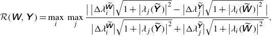 \begin{eqnarray} \mathcal{R}(\unicode{x1D652},\unicode{x1D654}{\kern2pt}) = \max _{i}\, \max _{j} \dfrac {{\big\lvert {\, {\big\lvert {\Delta {\lambda ^{\,\widetilde {\!{\kern-1pt}\unicode{x1D652}}}_i}}\big\rvert }\sqrt {1+{\big\lvert {\lambda _j({\,\widetilde {\!{\kern-1pt}\unicode{x1D654}}}{\kern2pt})}\big\rvert }^2}-{\big\lvert {\Delta {\lambda ^{\,\widetilde {\!{\kern-1pt}\unicode{x1D654}}}_j}}\big\rvert }\sqrt {1+{\big\lvert {\lambda _i({\,\widetilde {\!{\kern-1pt}\unicode{x1D652}}}{\kern2pt})}\big\rvert }^2} \ } \big\rvert }}{{\big\lvert {\Delta {\lambda ^{\,\widetilde {\!{\kern-1pt}\unicode{x1D652}}}_i}} \big\rvert }\sqrt {1+{\big\lvert {\lambda _j({\,\widetilde {\!{\kern-1pt}\unicode{x1D654}}}{\kern2pt})} \big\rvert }^2}+{\big\lvert {\Delta {\lambda ^{\,\widetilde {\!{\kern-1pt}\unicode{x1D654}}}_j}} \big\rvert }\sqrt {1+{\big\lvert {\lambda _i({\,\widetilde {\!{\kern-1pt}\unicode{x1D652}}}{\kern2pt})} \big\rvert }^2}}, \end{eqnarray}
where
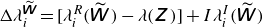 $\Delta {\lambda ^{\,\widetilde {\!{\kern-1pt}\unicode{x1D652}}}_i}= [\lambda ^R_i(\,\widetilde {\!{\kern-1pt}\unicode{x1D652}}{\kern2pt}) -\lambda (\unicode{x1D655}{\kern2pt}) ]+ I \lambda ^I_i(\,\widetilde {\!{\kern-1pt}\unicode{x1D652}}{\kern2pt})$
and
$\Delta {\lambda ^{\,\widetilde {\!{\kern-1pt}\unicode{x1D652}}}_i}= [\lambda ^R_i(\,\widetilde {\!{\kern-1pt}\unicode{x1D652}}{\kern2pt}) -\lambda (\unicode{x1D655}{\kern2pt}) ]+ I \lambda ^I_i(\,\widetilde {\!{\kern-1pt}\unicode{x1D652}}{\kern2pt})$
and
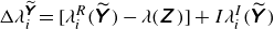 $\Delta {\lambda ^{\,\widetilde {\!{\kern-1pt}\unicode{x1D654}}}_i}= [\lambda ^R_i(\,\widetilde {\!{\kern-1pt}\unicode{x1D654}}{\kern2pt}) -\lambda (\unicode{x1D655}{\kern2pt}) ]+ I \lambda ^I_i(\,\widetilde {\!{\kern-1pt}\unicode{x1D654}}{\kern2pt})$
. The superscripts
$\Delta {\lambda ^{\,\widetilde {\!{\kern-1pt}\unicode{x1D654}}}_i}= [\lambda ^R_i(\,\widetilde {\!{\kern-1pt}\unicode{x1D654}}{\kern2pt}) -\lambda (\unicode{x1D655}{\kern2pt}) ]+ I \lambda ^I_i(\,\widetilde {\!{\kern-1pt}\unicode{x1D654}}{\kern2pt})$
. The superscripts
 $R$
and
$R$
and
 $I$
refer to real and imaginary components of the corresponding characteristics and
$I$
refer to real and imaginary components of the corresponding characteristics and
 $i,j=1,\ldots, 4$
are indices counting individual characteristics. Note that
$i,j=1,\ldots, 4$
are indices counting individual characteristics. Note that
 $\mathcal{R}(\unicode{x1D652},\unicode{x1D654}{\kern2pt})=\mathcal{R}(\unicode{x1D654},\unicode{x1D652}{\kern2pt})$
. The reader is referred to Appendix B.2 to see a further description and mathematical derivation of (4.8).
$\mathcal{R}(\unicode{x1D652},\unicode{x1D654}{\kern2pt})=\mathcal{R}(\unicode{x1D654},\unicode{x1D652}{\kern2pt})$
. The reader is referred to Appendix B.2 to see a further description and mathematical derivation of (4.8).
Equation (4.8) yields that under the condition where
 $\lambda ^R(\,\widetilde {\!{\kern-1pt}\unicode{x1D652}}{\kern2pt}) =\lambda ^R(\,\widetilde {\!{\kern-1pt}\unicode{x1D654}}{\kern2pt}) =\lambda (\unicode{x1D655}{\kern2pt})$
and
$\lambda ^R(\,\widetilde {\!{\kern-1pt}\unicode{x1D652}}{\kern2pt}) =\lambda ^R(\,\widetilde {\!{\kern-1pt}\unicode{x1D654}}{\kern2pt}) =\lambda (\unicode{x1D655}{\kern2pt})$
and
 $\lambda ^I(\,\widetilde {\!{\kern-1pt}\unicode{x1D654}}{\kern2pt})=\lambda ^I(\,\widetilde {\!{\kern-1pt}\unicode{x1D652}}{\kern2pt}) \gt 0$
, then
$\lambda ^I(\,\widetilde {\!{\kern-1pt}\unicode{x1D654}}{\kern2pt})=\lambda ^I(\,\widetilde {\!{\kern-1pt}\unicode{x1D652}}{\kern2pt}) \gt 0$
, then
 $\mathcal{R}(\unicode{x1D652},\unicode{x1D654}{\kern2pt})=0$
, which implies that long waves can resonantly interact since they are phase locked and have an equal growth rate. Therefore,
$\mathcal{R}(\unicode{x1D652},\unicode{x1D654}{\kern2pt})=0$
, which implies that long waves can resonantly interact since they are phase locked and have an equal growth rate. Therefore,
 $\mathcal{R} \rightarrow 0$
(note that
$\mathcal{R} \rightarrow 0$
(note that
 $0 \leqslant \mathcal{R} \leqslant 1$
) is a condition for near resonance, whereas when
$0 \leqslant \mathcal{R} \leqslant 1$
) is a condition for near resonance, whereas when
 $\mathcal{R} \rightarrow 1$
, long waves are not phase locked and do not resonate. Note that for the special case of pure exchange flow discussed in § 3.2.2, the
$\mathcal{R} \rightarrow 1$
, long waves are not phase locked and do not resonate. Note that for the special case of pure exchange flow discussed in § 3.2.2, the
 $F_1^2=F_{\varDelta +}^2$
condition that defines the neutral stability curve for long waves also leads to
$F_1^2=F_{\varDelta +}^2$
condition that defines the neutral stability curve for long waves also leads to
 $\lambda (\,\widetilde {\!{\kern-1pt}\unicode{x1D654}}{\kern2pt})=\lambda (\,\widetilde {\!{\kern-1pt}\unicode{x1D652}}{\kern2pt})$
, which corresponds to the resonance condition
$\lambda (\,\widetilde {\!{\kern-1pt}\unicode{x1D654}}{\kern2pt})=\lambda (\,\widetilde {\!{\kern-1pt}\unicode{x1D652}}{\kern2pt})$
, which corresponds to the resonance condition
 $\mathcal{R} = 0$
(since
$\mathcal{R} = 0$
(since
 $\lambda_1=\lambda_3$
and
$\lambda_1=\lambda_3$
and
 $\lambda_2=\lambda_4$
). Equivalently,
$\lambda_2=\lambda_4$
). Equivalently,
 $\mathcal{R} = 0$
marks the neutral stability of the long waves.
$\mathcal{R} = 0$
marks the neutral stability of the long waves.
This equivalence highlights a connection between the resonance mechanism and the onset of long-wave instability in pure exchange flows. For more general three-layer exchange flows, where the neutral stability curve cannot be expressed analytically, we expect the resonance measure
 $\mathcal{R}$
to continue to serve as a useful diagnostic for identifying resonant interactions between interfacial waves. To confirm this, we apply the
$\mathcal{R}$
to continue to serve as a useful diagnostic for identifying resonant interactions between interfacial waves. To confirm this, we apply the
 $\mathcal{R}$
measure to DNS data in the following section.
$\mathcal{R}$
measure to DNS data in the following section.
Contours of the long-wave resonance indicator
 $\mathcal{R}$
plotted in space–time
$\mathcal{R}$
plotted in space–time
 $(x, t)$
for the SW (a), TW (b) and I (c) cases. The dark regions indicate the minimum spectral gap, as defined in (4.8), between the perturbed upper and lower layers, derived from the building-block matrix decomposition of the three-layer system into perturbed upper and lower layer subsystems in (4.1).
$(x, t)$
for the SW (a), TW (b) and I (c) cases. The dark regions indicate the minimum spectral gap, as defined in (4.8), between the perturbed upper and lower layers, derived from the building-block matrix decomposition of the three-layer system into perturbed upper and lower layer subsystems in (4.1).
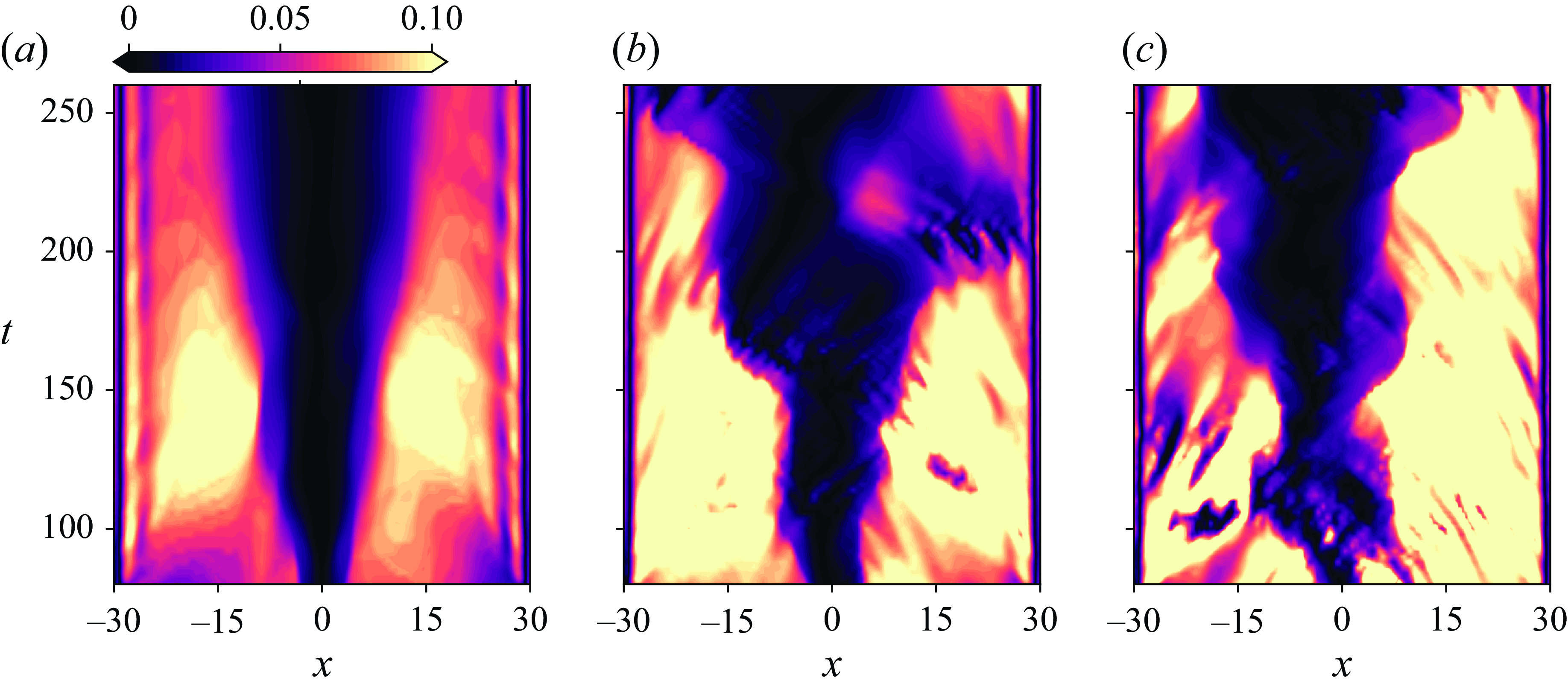
4.3.2. Application to the data
The contours of the long-wave resonance indicator
 $\mathcal{R}$
are shown in figure 12 for the SW, TW and I cases. All cases qualitatively correspond to the
$\mathcal{R}$
are shown in figure 12 for the SW, TW and I cases. All cases qualitatively correspond to the
 $\widetilde {G}$
contours in figure 9(d–f), particularly in the sense that the regime transitions from a supercritical hydraulic regime (
$\widetilde {G}$
contours in figure 9(d–f), particularly in the sense that the regime transitions from a supercritical hydraulic regime (
 $\widetilde {G} \gt 1$
) to a subcritical regime (
$\widetilde {G} \gt 1$
) to a subcritical regime (
 $\widetilde {G} \lt 1$
) when
$\widetilde {G} \lt 1$
) when
 $\mathcal{R} \approx 0$
. This similarity is noteworthy and not self-evident as the characteristics of the perturbed upper layer and those of the upper interface in the original three-layer flow are different by definition, i.e.
$\mathcal{R} \approx 0$
. This similarity is noteworthy and not self-evident as the characteristics of the perturbed upper layer and those of the upper interface in the original three-layer flow are different by definition, i.e.
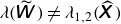 $\lambda (\,\widetilde {\!{\kern-1pt}\unicode{x1D652}}{\kern2pt}) \neq \lambda _{1,2}(\,\widehat {\!{\kern-1pt}\unicode{x1D653}}{\kern2pt})$
, and, similarly,
$\lambda (\,\widetilde {\!{\kern-1pt}\unicode{x1D652}}{\kern2pt}) \neq \lambda _{1,2}(\,\widehat {\!{\kern-1pt}\unicode{x1D653}}{\kern2pt})$
, and, similarly,
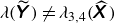 $\lambda (\,\widetilde {\!{\kern-1pt}\unicode{x1D654}}{\kern2pt}) \neq \lambda _{3,4}(\,\widehat {\!{\kern-1pt}\unicode{x1D653}}{\kern2pt})$
in general. Therefore, one would expect that
$\lambda (\,\widetilde {\!{\kern-1pt}\unicode{x1D654}}{\kern2pt}) \neq \lambda _{3,4}(\,\widehat {\!{\kern-1pt}\unicode{x1D653}}{\kern2pt})$
in general. Therefore, one would expect that
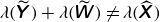 $\lambda (\,\widetilde {\!{\kern-1pt}\unicode{x1D654}}{\kern2pt}) + \lambda (\,\widetilde {\!{\kern-1pt}\unicode{x1D652}}{\kern2pt}) \neq \lambda (\,\widehat {\!{\kern-1pt}\unicode{x1D653}}{\kern2pt})$
. The striking resemblance between the spatiotemporal distributions of
$\lambda (\,\widetilde {\!{\kern-1pt}\unicode{x1D654}}{\kern2pt}) + \lambda (\,\widetilde {\!{\kern-1pt}\unicode{x1D652}}{\kern2pt}) \neq \lambda (\,\widehat {\!{\kern-1pt}\unicode{x1D653}}{\kern2pt})$
. The striking resemblance between the spatiotemporal distributions of
 $\mathcal{R}$
and
$\mathcal{R}$
and
 $\widetilde {G}$
suggests that the building-block decomposition introduced in § 4.2 provides valuable insight not only into the pathway for growth of interfacial waves but also their interactions and three-layer hydraulics. Moreover, it suggests that the hydraulic regime transition, driven by changes in the direction of information propagation along the interfaces, is also accompanied by long-wave resonance.
$\widetilde {G}$
suggests that the building-block decomposition introduced in § 4.2 provides valuable insight not only into the pathway for growth of interfacial waves but also their interactions and three-layer hydraulics. Moreover, it suggests that the hydraulic regime transition, driven by changes in the direction of information propagation along the interfaces, is also accompanied by long-wave resonance.
This long–long-wave resonance will modify the base state (mean flow) by the long waves themselves (figure 2). Such changes in the base state may lead to the onset of short-wave instabilities and result in the TKE generation at later times, as also found in Zhu et al. (Reference Zhu, Atoufi, Lefauve, Kerswell and Linden2024). For all cases, the contours of
 $\mathcal{R}$
are consistent with the TKE contours presented in figure 9 in the sense that strong TKE events are linked with interfacial wave resonances (i.e. the strong TKE occurs generally in places with the smallest
$\mathcal{R}$
are consistent with the TKE contours presented in figure 9 in the sense that strong TKE events are linked with interfacial wave resonances (i.e. the strong TKE occurs generally in places with the smallest
 $\mathcal{R}$
). A more detailed comparison between instantaneous profiles of TKE and
$\mathcal{R}$
). A more detailed comparison between instantaneous profiles of TKE and
 $\mathcal{R}$
is presented in Appendix C.
$\mathcal{R}$
is presented in Appendix C.
To properly establish the link between long-wave resonance and TKE generation, we also identify the resonance between long-wave and short-wave packets, eventually leading to the generation of small scales, which will be discussed next.
4.4. Indication of resonance between long and short waves
In this section we investigate the resonant interaction between long and short waves and provide evidence for the link between these interactions and the TKE. We begin by examining the connection between long- and short-wave instability in hydraulically controlled flow (§ 4.4.1). We then identify the conditions under which resonance between these waves can occur (§ 4.4.2). In § 4.4.3 we explore how such resonance contributes to turbulence generation, extending the analysis beyond linear wave stability. Finally, we apply the resulting diagnostics and criteria to DNS data in § 4.4.4.
4.4.1. Linking long-wave and short-wave instability: hydraulically controlled instability
In the previous section we examined the link between internal hydraulics and the instability of long waves. We now show that the stability of the entire wave spectrum – including short and intermediate waves – is likewise governed by the internal hydraulic state, characterised by the layer Froude numbers. This mechanism, which we refer to as hydraulically controlled instability, highlights that although the system is a stratified shear flow both the shear and stratification are prescribed by hydraulic conditions, which in turn control stability across all wavenumbers.
To illustrate this, we again consider the pure exchange flow case discussed in § 3.2.2, which simplifies the analysis. The imaginary components of the phase speeds of all waves in the spectrum, derived from the linear theory developed in Appendix A, are shown in figure 13. The top row corresponds to the bifurcation Froude number
 $F_{\varDelta -}^2$
and the bottom row to the marginal-stability Froude number
$F_{\varDelta -}^2$
and the bottom row to the marginal-stability Froude number
 $F_{\varDelta +}^2$
. As the Froude number increases from
$F_{\varDelta +}^2$
. As the Froude number increases from
 $F_{\varDelta -}^2$
to
$F_{\varDelta -}^2$
to
 $F_{\varDelta +}^2$
, the wave instability structure changes qualitatively across all wavenumbers – not just in the long-wave limit.
$F_{\varDelta +}^2$
, the wave instability structure changes qualitatively across all wavenumbers – not just in the long-wave limit.
Figure 13(a,b) shows that when
 $F_1^2 = F_{\varDelta -}^2$
, unstable modes span a broad wavenumber range – from long to short waves – up to
$F_1^2 = F_{\varDelta -}^2$
, unstable modes span a broad wavenumber range – from long to short waves – up to
 $k \lesssim 10$
, particularly in three-layer flows with a thick middle layer (
$k \lesssim 10$
, particularly in three-layer flows with a thick middle layer (
 $r \geqslant 1$
), where
$r \geqslant 1$
), where
 $r$
denotes the ratio of middle to upper layer thickness. Moreover, the phase speeds
$r$
denotes the ratio of middle to upper layer thickness. Moreover, the phase speeds
 $c_1$
and
$c_1$
and
 $c_4$
exhibit similar imaginary components across wavenumbers, indicating that interfacial waves at both interfaces grow at nearly the same rate. In contrast, when
$c_4$
exhibit similar imaginary components across wavenumbers, indicating that interfacial waves at both interfaces grow at nearly the same rate. In contrast, when
 $F_1^2 = F_{\varDelta +}^2$
, corresponding to marginal long-wave stability, instability is confined to short waves, which persist across a wide range of
$F_1^2 = F_{\varDelta +}^2$
, corresponding to marginal long-wave stability, instability is confined to short waves, which persist across a wide range of
 $r$
, as shown in figure 13(c,d). In this case, the
$r$
, as shown in figure 13(c,d). In this case, the
 $c_1^I$
and
$c_1^I$
and
 $c_4^I$
differ significantly, both in the values of
$c_4^I$
differ significantly, both in the values of
 $r$
that support instability and in the wavenumber ranges associated with peak
$r$
that support instability and in the wavenumber ranges associated with peak
 $c_1^I$
and
$c_1^I$
and
 $c_4^I$
, reflecting a decoupling of instability mechanisms across the layers.
$c_4^I$
, reflecting a decoupling of instability mechanisms across the layers.
These results suggest that the layer Froude numbers dictate both the onset and extent of instability across the wave spectrum. The observed similarity in the
 $c_1^I$
and
$c_1^I$
and
 $c_4^I$
in the
$c_4^I$
in the
 $F_1^2=F_{\varDelta -}^2$
case between long- and short-wave behaviour raises the question of whether these waves can interact resonantly – a possibility we now explore.
$F_1^2=F_{\varDelta -}^2$
case between long- and short-wave behaviour raises the question of whether these waves can interact resonantly – a possibility we now explore.
Instability map from contours of the imaginary component of the phase speed,
 $c^I$
, for linear disturbance waves in a three-layer pure exchange flow with a stagnant middle layer introduced in § 3.2.2. Both the bifurcation Froude number case
$c^I$
, for linear disturbance waves in a three-layer pure exchange flow with a stagnant middle layer introduced in § 3.2.2. Both the bifurcation Froude number case
 $F_1^2 = F_{\varDelta -}^2$
and the marginal-stability Froude number case
$F_1^2 = F_{\varDelta -}^2$
and the marginal-stability Froude number case
 $F_1^2 = F_{\varDelta +}^2$
defined in (3.16) are shown, isolating the dependence of wave amplification on the layer depth ratio
$F_1^2 = F_{\varDelta +}^2$
defined in (3.16) are shown, isolating the dependence of wave amplification on the layer depth ratio
 $r$
and wavenumber
$r$
and wavenumber
 $k$
. For
$k$
. For
 $F_{\varDelta -}^2$
, the interfacial modes
$F_{\varDelta -}^2$
, the interfacial modes
 $c_1$
and
$c_1$
and
 $c_4$
exhibit similar values of
$c_4$
exhibit similar values of
 $c^I$
, indicating comparable growth rates at both interfaces. In contrast, for
$c^I$
, indicating comparable growth rates at both interfaces. In contrast, for
 $F_{\varDelta +}^2$
, the growth characteristics differ between interfaces, with distinct ranges of
$F_{\varDelta +}^2$
, the growth characteristics differ between interfaces, with distinct ranges of
 $r$
and
$r$
and
 $k$
contributing to instability.
$k$
contributing to instability.
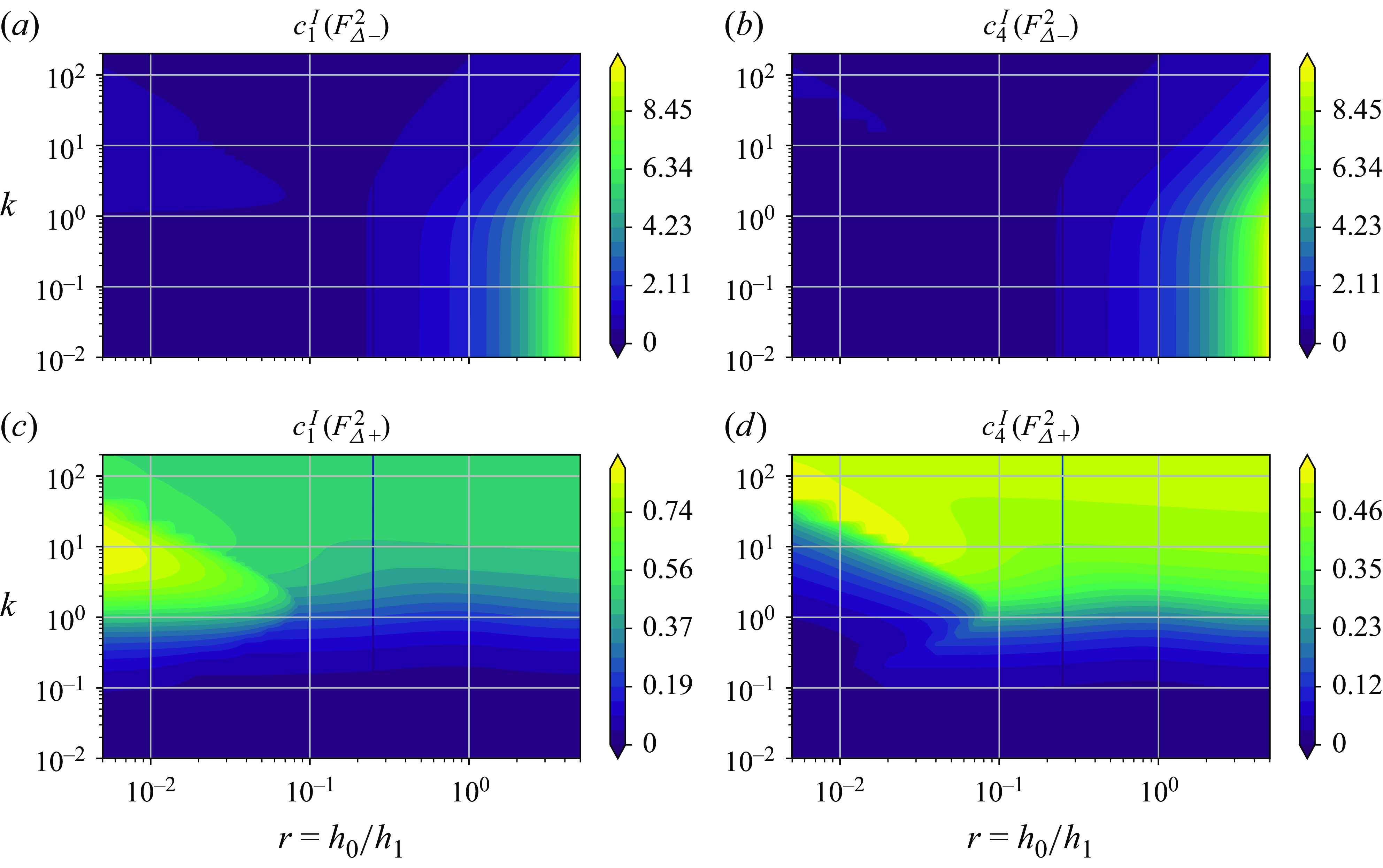
Imaginary component of the phase speed of the lower interfacial wave,
 $c_4^I$
, for pure exchange flow with a stagnant middle layer introduced in § 3.2.2 at selected wavenumbers
$c_4^I$
, for pure exchange flow with a stagnant middle layer introduced in § 3.2.2 at selected wavenumbers
 $k = 0.001$
(a),
$k = 0.001$
(a),
 $1$
(b) and
$1$
(b) and
 $10$
(c), plotted as a function of layer thickness ratio
$10$
(c), plotted as a function of layer thickness ratio
 $r$
and Froude number
$r$
and Froude number
 $F_1^2$
.
$F_1^2$
.
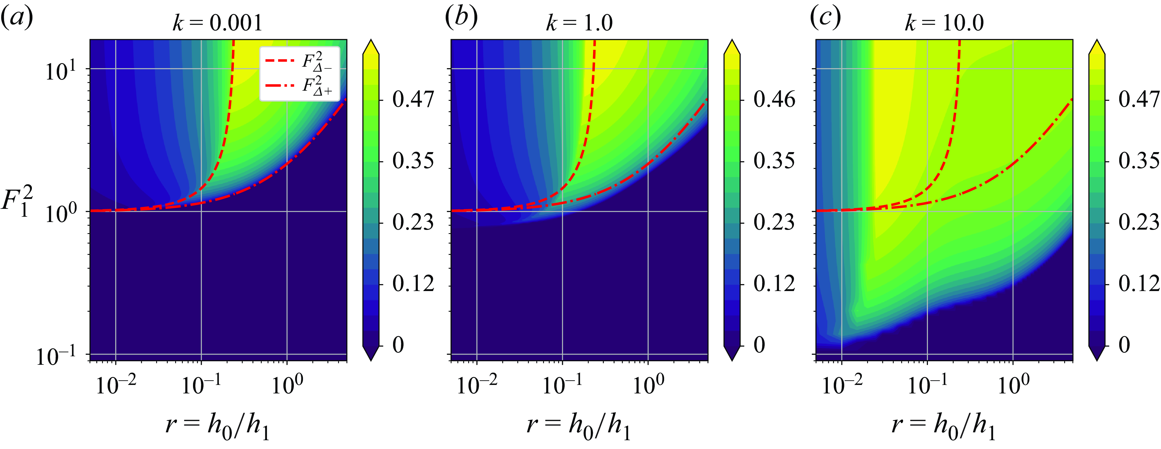
4.4.2. Resonance between long and short waves
To assess the potential for resonance between long and short waves, figure 14 shows
 $c_4^I$
for the pure exchange flow at selected wavenumbers (
$c_4^I$
for the pure exchange flow at selected wavenumbers (
 $k = 0.001$
,
$k = 0.001$
,
 $1$
and
$1$
and
 $10$
), across a range of layer thickness ratios
$10$
), across a range of layer thickness ratios
 $r$
and Froude numbers. At
$r$
and Froude numbers. At
 $k = 0.001$
shown in figure 14(a),
$k = 0.001$
shown in figure 14(a),
 $c_4^I$
closely matches its value in the long-wave limit (
$c_4^I$
closely matches its value in the long-wave limit (
 $k \to 0$
) shown previously in figure 13(b), confirming that the solution represents a long-wave mode. As can be seen from figure 14(a–c), for
$k \to 0$
) shown previously in figure 13(b), confirming that the solution represents a long-wave mode. As can be seen from figure 14(a–c), for
 $k \lt 1$
, the variation in phase speed as the wavenumber changes is relatively weak, while for
$k \lt 1$
, the variation in phase speed as the wavenumber changes is relatively weak, while for
 $k \gt 1$
, the phase speed continues to change significantly. This suggests that dispersion is strongest around
$k \gt 1$
, the phase speed continues to change significantly. This suggests that dispersion is strongest around
 $k = 1$
, where small differences in wavenumber lead to substantial differences in propagation speed. This behaviour implies that wave packets centred near
$k = 1$
, where small differences in wavenumber lead to substantial differences in propagation speed. This behaviour implies that wave packets centred near
 $k = 1$
are highly dispersive – that is, their constituent wavenumbers propagate at different phase speeds and, consequently, different group velocities. The implications of this for resonance and energy exchange will be explored in the following section. Additionally, increasing
$k = 1$
are highly dispersive – that is, their constituent wavenumbers propagate at different phase speeds and, consequently, different group velocities. The implications of this for resonance and energy exchange will be explored in the following section. Additionally, increasing
 $k$
broadens the region of instability as shown in figure 14(a–c), extending to lower Froude numbers (
$k$
broadens the region of instability as shown in figure 14(a–c), extending to lower Froude numbers (
 $F_1^2\lt F_{\varDelta +}^2$
) and a wider range of
$F_1^2\lt F_{\varDelta +}^2$
) and a wider range of
 $r$
, indicating that short-wave instability becomes more prominent where
$r$
, indicating that short-wave instability becomes more prominent where
 $F_1^2\lt F_{\varDelta +}^2$
.
$F_1^2\lt F_{\varDelta +}^2$
.
For systematic identification of resonance between long and short waves, let us recall that a packet of linear waves with phase velocity
 $c$
propagates at the group velocity,
$c$
propagates at the group velocity,
 \begin{equation} c_g= \frac {\partial (ck)}{\partial k}=c + k \frac {\partial c}{\partial k}=c+k d_g, \end{equation}
where
 $d_g = \partial c/\partial k$
measures the wave dispersivity. The kinetic energy is carried by the group velocity
$d_g = \partial c/\partial k$
measures the wave dispersivity. The kinetic energy is carried by the group velocity
 $c_g$
as the wave packet propagates, and
$c_g$
as the wave packet propagates, and
 $c$
is the phase velocity, whose mathematical expression is defined in Appendix A (from (A10)). Of particular interest is a packet of short waves with a group velocity close to the phase speed of the long waves (i.e.
$c$
is the phase velocity, whose mathematical expression is defined in Appendix A (from (A10)). Of particular interest is a packet of short waves with a group velocity close to the phase speed of the long waves (i.e.
 $c_g = \lambda$
), since long and short waves can then resonate (Ma Reference Ma1981).
$c_g = \lambda$
), since long and short waves can then resonate (Ma Reference Ma1981).
In general,
 $c \in \mathbb{C}$
, so
$c \in \mathbb{C}$
, so
 $c_g$
also contains real and imaginary parts. The real part
$c_g$
also contains real and imaginary parts. The real part
 $c_g^R$
represents the propagation speed of the wave envelope, while the imaginary part
$c_g^R$
represents the propagation speed of the wave envelope, while the imaginary part
 $c_g^I$
corresponds to its temporal growth. Resonance between wave packets and long interfacial waves is most likely when both
$c_g^I$
corresponds to its temporal growth. Resonance between wave packets and long interfacial waves is most likely when both
 $c_g^R \approx \lambda ^R$
and
$c_g^R \approx \lambda ^R$
and
 $c_g^I \approx \lambda ^I$
.
$c_g^I \approx \lambda ^I$
.
We utilise the general form of the spectral gap, as defined in (B13), to assess the relative group velocity of short wave packets compared with the phase speed of long waves at both the lower and upper interfaces. For a given wavenumber
 $k_0$
, we interpret the group velocity
$k_0$
, we interpret the group velocity
 $c_g|_{(k=k_0)} \in \mathbb{C}$
as the generalised eigenvalue of a perturbed matrix pair involving the three-layer matrix pair
$c_g|_{(k=k_0)} \in \mathbb{C}$
as the generalised eigenvalue of a perturbed matrix pair involving the three-layer matrix pair
 $\,\widehat {\!{\kern-1pt}\unicode{x1D653}} = (\unicode{x1D63C}, \unicode{x1D63E}{\kern2pt})$
, expressed as
$\,\widehat {\!{\kern-1pt}\unicode{x1D653}} = (\unicode{x1D63C}, \unicode{x1D63E}{\kern2pt})$
, expressed as
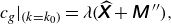 \begin{equation} {c_g|_{(k=k_0)} = \lambda (\,\widehat {\!{\kern-1pt}\unicode{x1D653}} + {\unicode{x1D648}{\kern2pt}''}),} \end{equation}
where
 $\unicode{x1D648}{\kern2pt}''$
is a perturbation matrix pair that accounts for the finite-wavenumber modulation of the wave packet. We recall that
$\unicode{x1D648}{\kern2pt}''$
is a perturbation matrix pair that accounts for the finite-wavenumber modulation of the wave packet. We recall that
 $\lambda (\,\widehat {\!{\kern-1pt}\unicode{x1D653}}{\kern2pt})$
yields the phase speed and growth rate of long interfacial waves in the three-layer flow, while
$\lambda (\,\widehat {\!{\kern-1pt}\unicode{x1D653}}{\kern2pt})$
yields the phase speed and growth rate of long interfacial waves in the three-layer flow, while
 $\lambda (\,\widehat {\!{\kern-1pt}\unicode{x1D653}} + {\unicode{x1D648}{\kern2pt}''})$
provides the corresponding quantities for the amplitude envelope of a wave packet centred around
$\lambda (\,\widehat {\!{\kern-1pt}\unicode{x1D653}} + {\unicode{x1D648}{\kern2pt}''})$
provides the corresponding quantities for the amplitude envelope of a wave packet centred around
 $k_0$
. Using this interpretation, we apply the spectral gap definition from (B13) to compute
$k_0$
. Using this interpretation, we apply the spectral gap definition from (B13) to compute
 \begin{equation} \mathcal{S} \equiv S_{\,\widehat {\!{\kern-1pt}\unicode{x1D653}}}({\unicode{x1D648}{\kern2pt}''}), \end{equation}
i.e. the spectral gap between long waves and short wave packets, by substituting
 $\unicode{x1D648} = \,\widehat {\!{\kern-1pt}\unicode{x1D653}}$
and
$\unicode{x1D648} = \,\widehat {\!{\kern-1pt}\unicode{x1D653}}$
and
 ${\unicode{x1D648}{\kern2pt}'} = {\unicode{x1D648}{\kern2pt}''}$
in (B13).
${\unicode{x1D648}{\kern2pt}'} = {\unicode{x1D648}{\kern2pt}''}$
in (B13).
The spectral gap
 $\mathcal{S}$
thus provides a diagnostic criterion for identifying near-resonant interactions between short-wave packets and long interfacial waves. Unlike the dispersion relation, which describes the behaviour of individual modes,
$\mathcal{S}$
thus provides a diagnostic criterion for identifying near-resonant interactions between short-wave packets and long interfacial waves. Unlike the dispersion relation, which describes the behaviour of individual modes,
 $\mathcal{S}$
quantifies the extent to which a short-wave packet can propagate at the same speed as a long wave. When this condition is met, efficient energy transfer from the long-wave to the short-wave packet becomes possible. In the next section we examine how this resonance mechanism contributes to turbulence generation, particularly through the amplification of short-wave disturbances in regions where
$\mathcal{S}$
quantifies the extent to which a short-wave packet can propagate at the same speed as a long wave. When this condition is met, efficient energy transfer from the long-wave to the short-wave packet becomes possible. In the next section we examine how this resonance mechanism contributes to turbulence generation, particularly through the amplification of short-wave disturbances in regions where
 $\mathcal{S}$
is small.
$\mathcal{S}$
is small.
4.4.3. The role of resonance in turbulence generation
The product
 $c_2^I c_4^I$
, shown in figure 17(c) for the TW and I cases, highlights regions in
$c_2^I c_4^I$
, shown in figure 17(c) for the TW and I cases, highlights regions in
 $(x, k)$
space where both interfacial modes are simultaneously unstable. These regions of modal amplification are especially pronounced for
$(x, k)$
space where both interfacial modes are simultaneously unstable. These regions of modal amplification are especially pronounced for
 $k \lesssim 1$
and spatially coincide with zones of elevated TKE in figure 9. Although the peak values of
$k \lesssim 1$
and spatially coincide with zones of elevated TKE in figure 9. Although the peak values of
 $c_2^I$
and
$c_2^I$
and
 $c_4^I$
do not occur at the same
$c_4^I$
do not occur at the same
 $x$
for all wavenumbers, their product effectively identifies regions of overlap where both modes contribute to instability. This spatial alignment suggests that energy amplification is not solely attributable to isolated modal growth, but may be enhanced by interactions between wave modes on both interfaces. In particular, simultaneous instability at the upper and lower interfaces permits resonant coupling between long interfacial waves and dispersive short-wave packets, enabling efficient energy transfer across scales.
$x$
for all wavenumbers, their product effectively identifies regions of overlap where both modes contribute to instability. This spatial alignment suggests that energy amplification is not solely attributable to isolated modal growth, but may be enhanced by interactions between wave modes on both interfaces. In particular, simultaneous instability at the upper and lower interfaces permits resonant coupling between long interfacial waves and dispersive short-wave packets, enabling efficient energy transfer across scales.
To understand the conditions that allow this energy transfer, we consider the limitations of the dispersion relation alone. While the dispersion relation derived in Appendix A plays a central role in identifying both long- and short-wave instabilities, it does not capture the interactions between modes at different scales. For instance, figure 17 shows that unstable modes exist on both interfaces over a broad wavenumber range. However, the dispersion relation does not indicate whether these modes are phase locked, whether their group velocities coincide or whether energy can be transferred between them.
This motivates the introduction of the spectral gap
 $\mathcal{S}$
, which quantifies the proximity between the group velocity of a short-wave packet and the phase speed of a long wave. When
$\mathcal{S}$
, which quantifies the proximity between the group velocity of a short-wave packet and the phase speed of a long wave. When
 $\mathcal{S} \rightarrow 0$
, a near-resonant condition is established: the short-wave packet is not only unstable but can also efficiently extract energy from long energetic waves. This leads to resonance-driven amplification of short-wave disturbances, even in parameter regimes where their modal instability alone may not explain the observed turbulence.
$\mathcal{S} \rightarrow 0$
, a near-resonant condition is established: the short-wave packet is not only unstable but can also efficiently extract energy from long energetic waves. This leads to resonance-driven amplification of short-wave disturbances, even in parameter regimes where their modal instability alone may not explain the observed turbulence.
4.4.4. Application to the data
To apply the theoretical framework developed above, we must select a representative wavenumber
 $k_0$
around which to evaluate the spectral gap
$k_0$
around which to evaluate the spectral gap
 $\mathcal{S}$
. This choice is guided by both dispersivity analysis and prior evidence of potential resonance. In particular, from the discussion in § 4.4.2, we have already seen that short-wave packets centred at
$\mathcal{S}$
. This choice is guided by both dispersivity analysis and prior evidence of potential resonance. In particular, from the discussion in § 4.4.2, we have already seen that short-wave packets centred at
 $k_0 = 1$
exhibit phase speeds comparable to those of long interfacial waves, suggesting conditions favourable for resonance.
$k_0 = 1$
exhibit phase speeds comparable to those of long interfacial waves, suggesting conditions favourable for resonance.
This is further supported by the dispersivity analysis shown in figure 18, which reveals that the wave dispersivity
 $|d_g|$
peaks at
$|d_g|$
peaks at
 $k_0 = 1$
, indicating the strongest dispersion and the wavenumber, therefore, is effective for coherent wave packet formation that carries energy through the flow. It is noteworthy that the dispersivity of small-amplitude long waves tends to zero as
$k_0 = 1$
, indicating the strongest dispersion and the wavenumber, therefore, is effective for coherent wave packet formation that carries energy through the flow. It is noteworthy that the dispersivity of small-amplitude long waves tends to zero as
 $k \rightarrow 0$
, since these waves are non-dispersive. In contrast, for short-wave packets, the dispersivity peaks at a wavenumber
$k \rightarrow 0$
, since these waves are non-dispersive. In contrast, for short-wave packets, the dispersivity peaks at a wavenumber
 $k_0$
, where
$k_0$
, where
 $|d_g|$
is maximal. Importantly, at
$|d_g|$
is maximal. Importantly, at
 $k_0 = 1$
, the phase speed
$k_0 = 1$
, the phase speed
 $c(k_0)$
remains
$c(k_0)$
remains
 $\mathcal{O}(1)$
, which is comparable to the long-wave phase speed
$\mathcal{O}(1)$
, which is comparable to the long-wave phase speed
 $\lambda$
. Furthermore, since
$\lambda$
. Furthermore, since
 $k_0 |d_g| \ll |c|$
, the group velocity
$k_0 |d_g| \ll |c|$
, the group velocity
 $c_g$
is close to
$c_g$
is close to
 $c$
, and hence, also comparable to
$c$
, and hence, also comparable to
 $\lambda$
. Therefore, wave packets centred at
$\lambda$
. Therefore, wave packets centred at
 $k_0=1$
travel at approximately the same speed as long waves, facilitating resonant coupling.
$k_0=1$
travel at approximately the same speed as long waves, facilitating resonant coupling.
Figure 15 shows space–time contours of
 $\mathcal{S}$
and demonstrates it qualitatively corresponds to
$\mathcal{S}$
and demonstrates it qualitatively corresponds to
 $\mathcal{R}$
and TKE for all cases despite their fundamentally different mathematical definitions. For example, figure 15(a,b) suggests that in the SW and TW cases,
$\mathcal{R}$
and TKE for all cases despite their fundamentally different mathematical definitions. For example, figure 15(a,b) suggests that in the SW and TW cases,
 $\mathcal{S}$
is smallest in the central regions of the duct and, therefore, the relative velocity between packets of short waves and long waves is small in this region. Consequently, in SID, in the central region where long interfacial waves are in near resonance, they also resonate with energy-carrying short-wave packets, amplifying the growth of the unstable short waves, resulting in breaking and generating small-scale turbulence and TKE. A more detailed comparison of the spatial distributions of TKE,
$\mathcal{S}$
is smallest in the central regions of the duct and, therefore, the relative velocity between packets of short waves and long waves is small in this region. Consequently, in SID, in the central region where long interfacial waves are in near resonance, they also resonate with energy-carrying short-wave packets, amplifying the growth of the unstable short waves, resulting in breaking and generating small-scale turbulence and TKE. A more detailed comparison of the spatial distributions of TKE,
 $\mathcal{R}$
and
$\mathcal{R}$
and
 $\mathcal{S}$
for the SW, TW and I cases at various times is presented in Appendix C.
$\mathcal{S}$
for the SW, TW and I cases at various times is presented in Appendix C.
Therefore,
 $\mathcal{S}$
and
$\mathcal{S}$
and
 $\mathcal{R}$
serve as complementary diagnostics to unravel the route to turbulence and small-scale generation in a stratified exchange flow such as SID. The next section summarises these mechanisms.
$\mathcal{R}$
serve as complementary diagnostics to unravel the route to turbulence and small-scale generation in a stratified exchange flow such as SID. The next section summarises these mechanisms.
4.5. Summary: resonance indicators and turbulence generation in space-time
In § 4.3 we introduced the indicator
 $\mathcal{R}$
to quantify the long–long wave resonance, which we associate with large-scale energy transfer and the onset of instability in hydraulically controlled three-layer flows. This process is distinct from subcritical-to-supercritical hydraulic transitions, which do not require instability and are well known from single-layer theory. In § 4.4 we introduced
$\mathcal{R}$
to quantify the long–long wave resonance, which we associate with large-scale energy transfer and the onset of instability in hydraulically controlled three-layer flows. This process is distinct from subcritical-to-supercritical hydraulic transitions, which do not require instability and are well known from single-layer theory. In § 4.4 we introduced
 $\mathcal{S}$
to indicate small-scale generation through short-wave instability (long–short wave resonance). As shown in figures 12 and 15, both
$\mathcal{S}$
to indicate small-scale generation through short-wave instability (long–short wave resonance). As shown in figures 12 and 15, both
 $\mathcal{R}$
and
$\mathcal{R}$
and
 $\mathcal{S}$
have similar spatiotemporal distributions and both are consistent with the TKE distribution (see also Appendix C). Therefore, both long–long wave and long–short wave (packet) resonance contribute to the TKE and, consequently, influence the onset of turbulence in SID. The close similarity between the
$\mathcal{S}$
have similar spatiotemporal distributions and both are consistent with the TKE distribution (see also Appendix C). Therefore, both long–long wave and long–short wave (packet) resonance contribute to the TKE and, consequently, influence the onset of turbulence in SID. The close similarity between the
 $x$
–
$x$
–
 $t$
distributions of
$t$
distributions of
 $\mathcal{R}$
and
$\mathcal{R}$
and
 $\mathcal{S}$
suggests an intrinsic connection between them, despite their fundamentally different mathematical definitions.
$\mathcal{S}$
suggests an intrinsic connection between them, despite their fundamentally different mathematical definitions.
The resonance between long waves and short-wave packets measured by
 $\mathcal{S}$
from (4.11): the spectral gap between most dispersive short-wave packets (i.e. wavenumbers centring around
$\mathcal{S}$
from (4.11): the spectral gap between most dispersive short-wave packets (i.e. wavenumbers centring around
 $k \approx 1$
) and long waves in (a) SW, (b) TW and (c) I cases.
$k \approx 1$
) and long waves in (a) SW, (b) TW and (c) I cases.
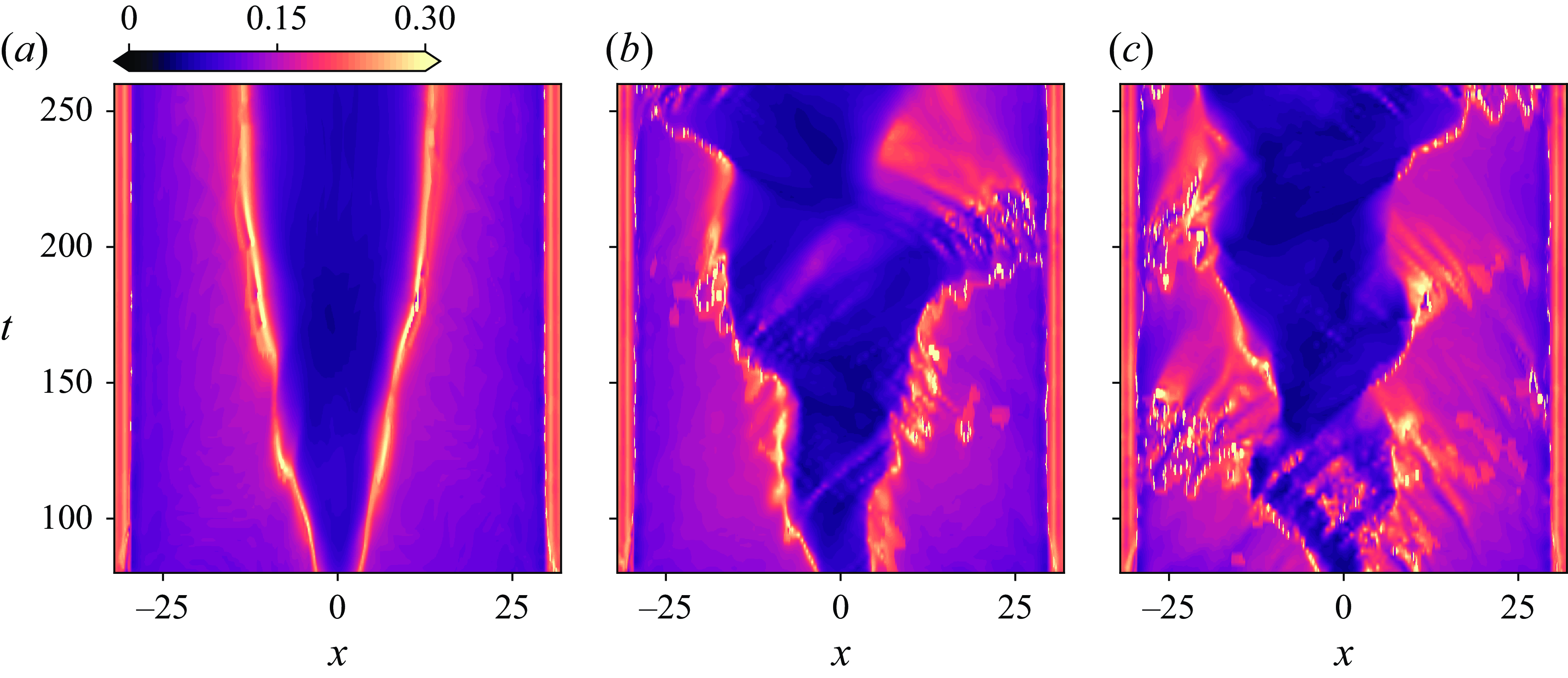
Conceptual profiles illustrating the instantaneous resonance indicators for long–long wave (
 $\mathcal{R}$
) and long–short wave packet (
$\mathcal{R}$
) and long–short wave packet (
 $\mathcal{S}$
) interactions, shown alongside TKE for comparison. The parameter
$\mathcal{S}$
) interactions, shown alongside TKE for comparison. The parameter
 $A$
represents the length-to-height aspect ratio of the stratified exchange flow considered here.
$A$
represents the length-to-height aspect ratio of the stratified exchange flow considered here.
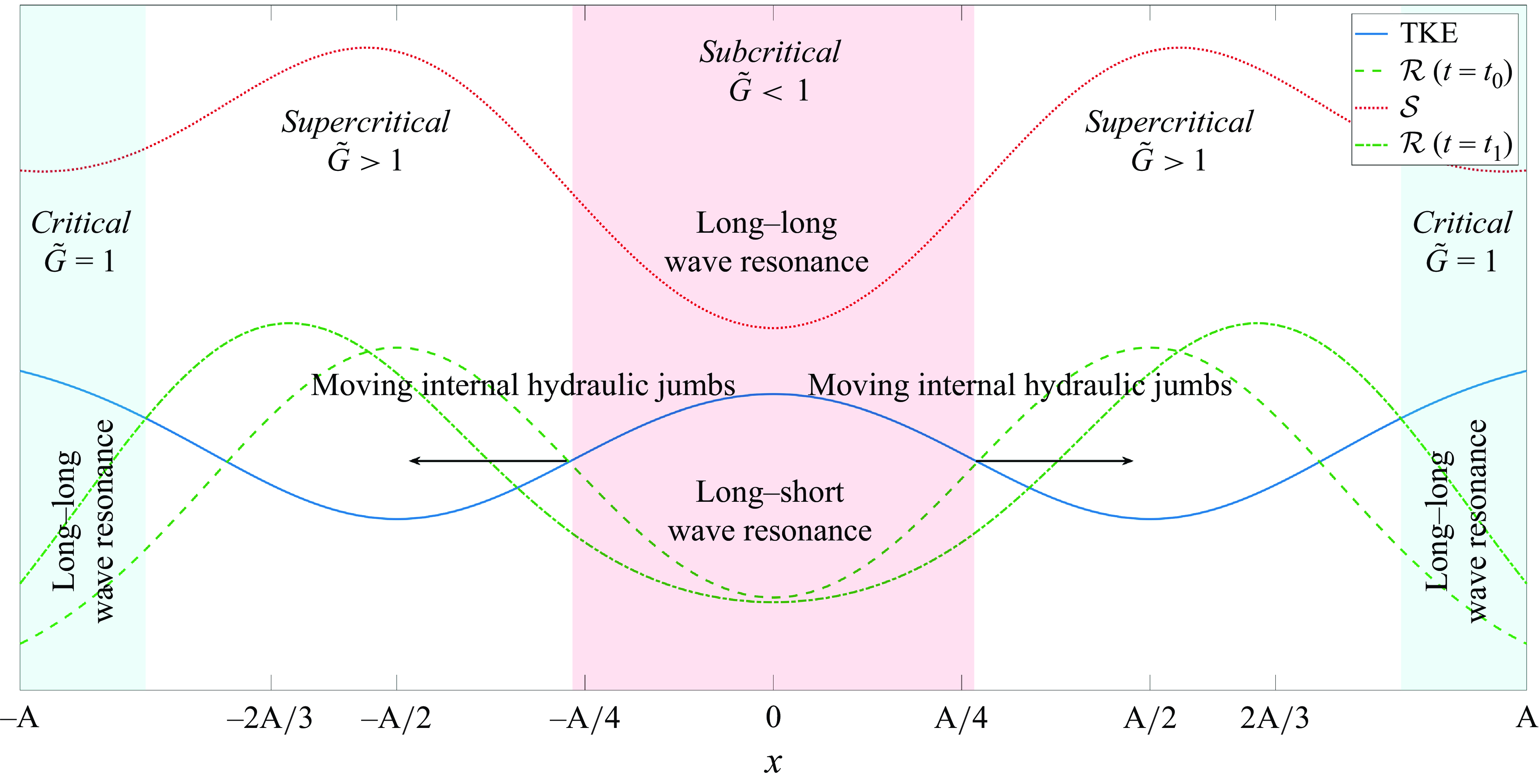
This process is also interpreted through the vertical structure of the wave modes. Long waves refer to disturbances with a small horizontal wavenumber
 $k$
, corresponding to large-scale structures in the streamwise (
$k$
, corresponding to large-scale structures in the streamwise (
 $x$
) direction. Because they vary slowly in
$x$
) direction. Because they vary slowly in
 $x$
, the associated pressure and velocity perturbations extend over the full vertical depth of the duct, leading to broad vertical mode structures that align well with the background shear
$x$
, the associated pressure and velocity perturbations extend over the full vertical depth of the duct, leading to broad vertical mode structures that align well with the background shear
 $U(z)$
. This vertical coherence allows long waves to efficiently extract energy from the mean flow. However, their smooth structure induces weak vertical gradients, making them ineffective at generating localised shear or mixing across density interfaces.
$U(z)$
. This vertical coherence allows long waves to efficiently extract energy from the mean flow. However, their smooth structure induces weak vertical gradients, making them ineffective at generating localised shear or mixing across density interfaces.
Short waves, in contrast, are associated with a large horizontal wavenumber
 $k$
and are confined near the density interfaces, with vertical structures that decay rapidly away from these regions. Although their projection onto the background shear is weaker, limiting their ability to extract energy directly from the mean flow, they can generate sharp interfacial gradients that enhance local shear and promote mixing. Thus, they are more effective at driving the small-scale turbulent structures responsible for mixing across layers.
$k$
and are confined near the density interfaces, with vertical structures that decay rapidly away from these regions. Although their projection onto the background shear is weaker, limiting their ability to extract energy directly from the mean flow, they can generate sharp interfacial gradients that enhance local shear and promote mixing. Thus, they are more effective at driving the small-scale turbulent structures responsible for mixing across layers.
A key point revealed by our analysis is that long–short wave resonance enables a (nonlinear) energy transfer from long waves to short waves. In regions where both
 $\mathcal{R}$
and
$\mathcal{R}$
and
 $\mathcal{S}$
are minimised, long waves that have extracted energy from the mean flow can resonantly transfer energy to short waves, thereby amplifying them and facilitating intense mixing. This interaction contributes to the observed generation of TKE and mixing in the middle layer.
$\mathcal{S}$
are minimised, long waves that have extracted energy from the mean flow can resonantly transfer energy to short waves, thereby amplifying them and facilitating intense mixing. This interaction contributes to the observed generation of TKE and mixing in the middle layer.
This interpretation is supported by the qualitative similarity of low
 $\mathcal{R}$
and
$\mathcal{R}$
and
 $\mathcal{S}$
values with regions of enhanced TKE, as well as by previous theoretical work on long-wave-induced instability in exchange flows (Zhu et al. Reference Zhu, Atoufi, Lefauve, Kerswell and Linden2024). Together, these observations demonstrate the complementary roles of long and short waves in driving the transition to turbulence in stratified exchange flows such as SID.
$\mathcal{S}$
values with regions of enhanced TKE, as well as by previous theoretical work on long-wave-induced instability in exchange flows (Zhu et al. Reference Zhu, Atoufi, Lefauve, Kerswell and Linden2024). Together, these observations demonstrate the complementary roles of long and short waves in driving the transition to turbulence in stratified exchange flows such as SID.
The schematic profile in figure 16 illustrates the spatial distribution of long–long and long–short wave resonances within the SID flow, integrating the space–time interactions shown in figures 12 and 15 and comparing them with the TKE distribution presented in figure 9(a–c). This schematic also incorporates the spatial profiles in figure 20 and the analysis in Appendix C, providing insights into the identification of wave resonances and the hydraulic transition to turbulence. In the wave cases, as well as during the quiet phase of the I case, critical regions near the duct ends (where
 $\widetilde {G} \approx 1$
) are observed, where the lowest values of
$\widetilde {G} \approx 1$
) are observed, where the lowest values of
 $\mathcal{R}$
coincide with the strongest TKE, while
$\mathcal{R}$
coincide with the strongest TKE, while
 $\mathcal{S}$
remains minimised. This pattern suggests that hydraulic transition and TKE generation are primarily driven by long–long wave resonance, in conjunction with short-wave instabilities at the upper and lower interfaces without substantial resonant interactions. In the duct centre (subcritical region where
$\mathcal{S}$
remains minimised. This pattern suggests that hydraulic transition and TKE generation are primarily driven by long–long wave resonance, in conjunction with short-wave instabilities at the upper and lower interfaces without substantial resonant interactions. In the duct centre (subcritical region where
 $\widetilde {G} \lt 1$
), both long–long and long–short wave resonances coexist, facilitating the hydraulic transition to turbulence. As the central hydraulic jumps progress toward the duct ends and the subcritical region expands, these regions of resonant interaction grow, occupying an increasingly extensive portion of the duct.
$\widetilde {G} \lt 1$
), both long–long and long–short wave resonances coexist, facilitating the hydraulic transition to turbulence. As the central hydraulic jumps progress toward the duct ends and the subcritical region expands, these regions of resonant interaction grow, occupying an increasingly extensive portion of the duct.
4.6. Application to oceanic flows
The theoretical framework developed in this study, based on three-layer hydraulic analysis and the diagnosing resonant interactions between long and short waves, can be applied to stratified exchange flows in the ocean. These include confined regions like straits, estuaries, fjords, canyons and semi-enclosed basins, where salinity and/or temperature stratification often create three-layer flows governed by hydraulic controls. A notable example is the Bosphorus Strait, linking the Black Sea and the Mediterranean, where bathymetric constriction and density differences support layered, hydraulically controlled stratified exchange. Below, we outline several potential applications.
4.6.1. Implementations for adaptive resolution in ocean models
Recent advances in high-resolution numerical ocean modelling, particularly the lat-lon-cap (LLC) simulations such as LLC4320 (Gallmeier et al. Reference Gallmeier, Su, Rocha, Menemenlis and Klein2023), have enabled global ocean simulations at approximately
 $1/48^{\circ }$
horizontal resolution (
$1/48^{\circ }$
horizontal resolution (
 $\sim\! 2$
km at the equator) using the Massachusetts Institute of Technology general circulation model (MITgcm). Despite this relatively high spatial resolution, turbulence is far from being resolved, and mixing remains parameterised through local gradient-based closures.
$\sim\! 2$
km at the equator) using the Massachusetts Institute of Technology general circulation model (MITgcm). Despite this relatively high spatial resolution, turbulence is far from being resolved, and mixing remains parameterised through local gradient-based closures.
The diagnostic measures
 $\mathcal{R}$
and
$\mathcal{R}$
and
 $\mathcal{S}$
developed in this study quantify the conditions under which long waves resonate with dispersive short-wave packets. Since these diagnostics rely only on layer-averaged quantities – velocities, densities and interface displacements – they are directly applicable to model outputs.
$\mathcal{S}$
developed in this study quantify the conditions under which long waves resonate with dispersive short-wave packets. Since these diagnostics rely only on layer-averaged quantities – velocities, densities and interface displacements – they are directly applicable to model outputs.
In coastal and marginal seas, particularly in estuarine and strait-like geometries where the Rossby number is large and rotational effects are weak, the three-layer approximation proposed in this study is especially appropriate. Our results imply that even without directly resolving turbulence, ocean models can leverage these diagnostics to identify zones of intensified TKE generation. This insight may be valuable for implementing adaptive mesh refinement in regional models, where local grid refinement could be concentrated in dynamically active zones suggested by long–short wave resonance conditions. Because all diagnostic expressions derived here are analytical, this integration poses no additional computational burden and presents a promising route toward physics-informed resolution enhancement in estuarine and strait flows.
4.6.2. Implications for mixing parametrisation
While in this study we applied the theoretical framework to DNS datasets of SID flows, the methodology can be extended to ocean circulation models, which typically solve shallow water or layer-averaged primitive equations. These models do not resolve turbulence explicitly and usually assume hydrostatic balance, thus neglecting non-hydrostatic pressure gradients that play a key role in wave-driven turbulence and mixing.
The model output can be decomposed into three effective layers by discretising the vertical structure into bulk velocity, density and thickness in each layer via appropriate integration. These layer-averaged quantities serve as input to the theory developed here, enabling the computation of resonance diagnostics
 $\mathcal{R}$
and
$\mathcal{R}$
and
 $\mathcal{S}$
, the linear wave speed
$\mathcal{S}$
, the linear wave speed
 $c$
, the imaginary part
$c$
, the imaginary part
 $c_i$
as a proxy for instability and the dispersivity
$c_i$
as a proxy for instability and the dispersivity
 $|d_g|$
, defined as the magnitude of the group velocity derivative with respect to wavenumber. In regions where
$|d_g|$
, defined as the magnitude of the group velocity derivative with respect to wavenumber. In regions where
 $\mathcal{S}$
is locally minimum or
$\mathcal{S}$
is locally minimum or
 $|d_g|$
is large, we suggest that turbulent viscosity in mixing parametrisations could adopt a velocity scale based on the group velocity of the most dispersive wave packet,
$|d_g|$
is large, we suggest that turbulent viscosity in mixing parametrisations could adopt a velocity scale based on the group velocity of the most dispersive wave packet,
 $c_g(k_0)$
, where
$c_g(k_0)$
, where
 $k_0$
corresponds to the wavenumber at which
$k_0$
corresponds to the wavenumber at which
 $|d_g|$
peaks.
$|d_g|$
peaks.
This provides a leading-order correction to existing mixing schemes that rely solely on local shear or stratification. It leverages the resolved mean state of an ocean model to estimate non-hydrostatic, wave-induced pathways to turbulence, which are otherwise absent in hydrostatic model formulations. Consequently, it offers a route to enhance parametrisation schemes with minimal computational overhead while capturing key non-local mixing mechanisms.
4.7. Outlook
The good agreement between DNS and temperature-stratified shadowgraph experiments in Zhu et al. (Reference Zhu, Atoufi, Lefauve, Taylor, Kerswell, Dalziel, Lawrence and Linden2023) suggests that hydraulic effects, including both long–long and long–short wave interactions, play an important role in these experiments. Furthermore, recent augmented experimental data (Zhu et al. Reference Zhu, Atoufi, Lefauve, Kerswell and Linden2024) from salt-stratified experiments using physics-informed neural networks and the reconstructed pressure field indicates that the offset of the density interface, and thus, the asymmetry in short (Holmboe) waves are also caused by hydraulic effects. However, the question of how the Prandtl number influences these interactions remains open.
A promising direction for future work is the inclusion of a steady or oscillatory barotropic background flow. In many geophysical contexts, particularly in estuaries and straits, the exchange flow is influenced by persistent barotropic currents or low-frequency tidal forcing. A key assumption in the present formulation is that the net volume flux vanishes, i.e.
 $u_1 h_1 + u_2 h_2 + u_0 h_0 = 0$
. In the presence of barotropic forcing, this condition generalises to
$u_1 h_1 + u_2 h_2 + u_0 h_0 = 0$
. In the presence of barotropic forcing, this condition generalises to
 $u_1 h_1 + u_2 h_2 + u_0 h_0 = Q(x,t)$
, where
$u_1 h_1 + u_2 h_2 + u_0 h_0 = Q(x,t)$
, where
 $Q$
is a prescribed barotropic volume flux. This introduces spatiotemporal variability into the base state and alters the characteristics of the three-layer flow. Consequently, resonance conditions and growth rates become time dependent on the scale relevant to the forcing time scale, potentially modifying the nature and location of mixing.
$Q$
is a prescribed barotropic volume flux. This introduces spatiotemporal variability into the base state and alters the characteristics of the three-layer flow. Consequently, resonance conditions and growth rates become time dependent on the scale relevant to the forcing time scale, potentially modifying the nature and location of mixing.
Another natural extension is to incorporate rotation. While the present study assumes non-rotating flows – a valid assumption in narrow, laterally confined geometries – large-scale oceanic flows are influenced by Coriolis effects, including continental shelf regions, curved straits and deep ocean canyons. Including rotation would introduce geostrophic balance into the mean flow and modify the structure of internal wave characteristics. This could suppress or enhance wave interactions depending on the local Rossby number and geometry.
These extensions, accounting for barotropic variability and rotational effects, represent important steps toward adapting the resonance-based framework developed here into a more general predictive tool for mixing in real oceanic flows.
5. Conclusions
This paper has discussed the three-layer hydraulics of stratified exchange flows in inclined ducts and significantly improved upon the two-layer hydraulics of Atoufi et al. (Reference Atoufi, Zhu, Lefauve, Taylor, Kerswell, Dalziel, Lawrence and Linden2023). The improvement lies in the inclusion of viscous effects, non-hydrostatic pressure gradients and a third mixed layer in the quantitative analysis of the internal hydraulics and wave instabilities, which is generalisable to any three-layer exchange flows with mixing.
We first introduced the viscous three-layer-averaged equations with non-hydrostatic pressure gradients and mixing. We then provided expressions for the eigenvalues of the homogeneous system of equations (i.e. characteristics) and the propagation of information, and defined a composite Froude number based on the characteristics of the three-layer flows. While related formulations have appeared in prior work, this approach based on characteristics has not, to our knowledge, been previously reported. Unlike two-layer hydraulics, three-layer hydraulics predict a subcritical/critical region, separated by two hydraulic control points, within which flow transitions from supercritical to subcritical, and is accompanied by TKE generation. We have shown theoretically that the imaginary component of characteristics represents the growth rate of the linear long waves propagating on a background three-layer flow.
The system was then decomposed into three isolated layers through matrix decomposition, where the characteristics are strictly real. We demonstrated that long-wave growth occurs when interactions between these isolated layers are allowed. From this decomposition, perturbed upper and lower layers were defined resulting from the interaction between the isolated upper and lower layers, and influenced by the isolated middle layer. The spatiotemporal TKE was linked to long-wave resonance by quantifying the spectral gaps between the characteristics of the perturbed upper and lower layers. Additionally, we connected TKE to the resonance of dispersive short-wave packets carrying energy, characterised by a wavelength three times the duct height, whose group velocity drives kinetic energy transfer.
The first turbulent transition mechanism arises when long waves have identical speeds and growth rates, facilitating resonance between them. In this case, the spectral gap between the perturbed upper and lower layers vanishes. Such a resonant interaction also changes the base state around which the perturbation evolves and triggers instabilities. The next mechanism arises when long waves directly interact with a packet of dispersive short waves, where the phase speed and growth rate of their amplitude envelope are equal to those of long interfacial waves. In this case, direct interactions between long and short waves trigger instability and the generation of smaller scales.
This paper has focused on the three regimes identified in Zhu et al. (Reference Zhu, Atoufi, Lefauve, Taylor, Kerswell, Dalziel, Lawrence and Linden2023): stationary and travelling wave regimes (SW and TW case) together with the intermittently turbulent regime (I case). We provided the first evidence from three-dimensional DNS datasets that strong TKE correlates with long–long waves and long–short wave packet resonance. We deduce that the transition to turbulence in stratified exchange flow exhibits a high degree of non-locality owing to resonant interactions between long and short waves. The parametrisation of mixing in applications, including in the ocean, is often based on local gradients of the flow. This paper underscores the need to revisit modelling strategies to account for non-local pathways to turbulence, especially in situations where the flow is hydraulically controlled or influenced, and susceptible to long-wave instability (e.g. in estuaries and straits).
Funding
We acknowledge support from the European Research Council (ERC) under the European Union’s Horizon 2020 research and innovation Grant No 742480 ‘Stratified Turbulence And Mixing Processes’ (STAMP). Parts of the simulations were carried out with resources from Compute/Calcul Canada. A.L. is funded by a NERC Independent Research Fellowship (NE/W008971/1). For the purpose of open access, the authors have applied a Creative Commons Attribution (CC BY) licence to any Author Accepted Manuscript version arising from this submission.
Declaration of interests
The authors report no conflict of interest.
Appendix A. Linear instabilities and the link to three-layer hydraulics
We assume three-layer piecewise constant base velocity and density profiles of the form
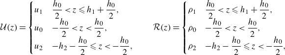 \begin{eqnarray} \mathcal{U}(z)= \begin{cases} u_1 & \dfrac {h_0}{2} \lt z \leqslant h_1+\dfrac {h_0}{2},\\ u_0 & -\dfrac {h_0}{2} \lt z \lt \dfrac {h_0}{2}, \\ u_2 & -h_2-\dfrac {h_0}{2} \leqslant z \lt -\dfrac {h_0}{2}, \end{cases} \qquad \mathcal{R}(z)= \begin{cases} \rho _1 & \dfrac {h_0}{2} \lt z \leqslant h_1+\dfrac {h_0}{2},\\ \rho _0 & -\dfrac {h_0}{2} \lt z \lt \dfrac {h_0}{2}, \\ \rho _2 & -h_2-\dfrac {h_0}{2} \leqslant z \lt -\dfrac {h_0}{2}, \end{cases} \end{eqnarray}
where we use layer-average quantities from DNS data to compute
 $\mathcal{U}(z)$
and
$\mathcal{U}(z)$
and
 $\mathcal{R}(z)$
. We add a perturbation streamfunction of the form
$\mathcal{R}(z)$
. We add a perturbation streamfunction of the form
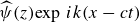 $\widehat {\psi }(z) \textrm{exp}\, \, ik(x-ct)$
to represent linear disturbance waves propagating in a background flow with prescribed
$\widehat {\psi }(z) \textrm{exp}\, \, ik(x-ct)$
to represent linear disturbance waves propagating in a background flow with prescribed
 $\mathcal{U}(z)$
and
$\mathcal{U}(z)$
and
 $\mathcal{R}(z)$
. We implicitly assume that the above parallel base flow is a good model for exchange flows varying slowly along
$\mathcal{R}(z)$
. We implicitly assume that the above parallel base flow is a good model for exchange flows varying slowly along
 $x$
compared with the wavelength of the perturbation. The evolution of the perturbation inside the duct (away from the inlet/outlet) is given by the forced Taylor–Goldstein equation (TGE) (Atoufi et al. Reference Atoufi, Zhu, Lefauve, Taylor, Kerswell, Dalziel, Lawrence and Linden2023):
$x$
compared with the wavelength of the perturbation. The evolution of the perturbation inside the duct (away from the inlet/outlet) is given by the forced Taylor–Goldstein equation (TGE) (Atoufi et al. Reference Atoufi, Zhu, Lefauve, Taylor, Kerswell, Dalziel, Lawrence and Linden2023):
 \begin{eqnarray}\!\!\!\! \left [\left (\mathcal{U}-c\right )\widehat {\psi }'-\mathcal{U}'\widehat {\psi } \right ]'-\left (\mathcal{U}-c\right ) k^2 \widehat {\psi } - \frac {{Ri} \cos {\theta } \ \mathcal{R}'}{\mathcal{U}-c} \widehat {\psi } = - \frac {i}{k} {Ri} \sin {\theta } \ \left [ \frac {\mathcal{R'} \widehat {\psi }}{\mathcal{U}-c} \right ]^{\prime}, \end{eqnarray}
where primes denote
 $d/{\rm d}z$
. For the three-layer base flow (A1),
$d/{\rm d}z$
. For the three-layer base flow (A1),
 $\mathcal{U''}=\mathcal{R'}=0$
everywhere except at the interface, the TGE (A2) reduces to
$\mathcal{U''}=\mathcal{R'}=0$
everywhere except at the interface, the TGE (A2) reduces to
 \begin{eqnarray} \widehat {\psi }''-k^2 \widehat {\psi }=0 \end{eqnarray}
everywhere except at the lower and upper interfaces and we therefore seek the solution of the form
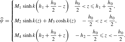 \begin{eqnarray} \widehat {\psi }= \begin{cases} M_1 \sinh {k \bigg(h_1+\dfrac {h_0}{2}-z\bigg)}\quad \dfrac {h_0}{2} \lt z \leqslant h_1+\dfrac {h_0}{2}, \\[10pt] M_2 \sinh {k (z)} + M_3 \cosh {k (z)}\quad -\dfrac {h_0}{2} \lt z \lt \dfrac {h_0}{2}, \\[10pt] M_4 \sinh {k \bigg(h_2+\dfrac {h_0}{2}+z\bigg)}\quad -h_2-\dfrac {h_0}{2} \leqslant z \lt -\dfrac {h_0}{2}. \end{cases} \end{eqnarray}
We note this solution satisfies the impermeability condition at
 $z=-h_2-({h_0}/{2})$
and
$z=-h_2-({h_0}/{2})$
and
 $z=h_1+({h_0}/{2})$
where
$z=h_1+({h_0}/{2})$
where
 $\widehat {w} =i k\widehat {\psi }=0$
since the vertical velocity of the disturbance waves vanishes at the upper and lower boundaries. We also note that
$\widehat {w} =i k\widehat {\psi }=0$
since the vertical velocity of the disturbance waves vanishes at the upper and lower boundaries. We also note that
 \begin{equation} \begin{aligned} \mathcal{U}'&=(u_1-u_0) \ \delta \left(z-\dfrac {h_0}{2}\right)+(u_0-u_2) \ \delta \left(z+\dfrac {h_0}{2}\right), \\ \mathcal{R}'&= (\rho _1-\rho _0) \ \delta \left(z-\dfrac {h_0}{2}\right)+(\rho _0-\rho _2) \ \delta \left(z+\dfrac {h_0}{2}\right), \end{aligned}\end{equation}
where
 $\delta$
is the Dirac delta function and
$\delta$
is the Dirac delta function and
 $\mathcal{U}''=\mathcal{R}'=0$
everywhere except at the lower and upper interfaces. The matching conditions are derived by integrating (A2) over the neighbourhood of the lower and upper interfaces (
$\mathcal{U}''=\mathcal{R}'=0$
everywhere except at the lower and upper interfaces. The matching conditions are derived by integrating (A2) over the neighbourhood of the lower and upper interfaces (
 $z=\pm {h_0}/{2}$
) leading to
$z=\pm {h_0}/{2}$
) leading to
 \begin{equation}\begin{aligned} \left[\left[ \frac {\widehat {\psi }}{\mathcal{U}-c} \right]\right]_{\eta _i}&=0, \\ \left[\left[ (\mathcal{U}-c)\widehat {\psi }' \right]\right]_{\eta _i} + g_i \left ( \frac {\widehat {\psi }}{\mathcal{U}-c} \right )_{z=\eta _i}&=0,\end{aligned} \end{equation}
where
 $\eta _i$
(
$\eta _i$
(
 $i=1,2$
) refers to lower and upper interface locations as determined in § 2.2. In deriving the matching conditions (A6) we also considered the small angle limit where
$i=1,2$
) refers to lower and upper interface locations as determined in § 2.2. In deriving the matching conditions (A6) we also considered the small angle limit where
 $\sin (\theta ) \ll \cos {\theta }$
and neglected the right-hand side of (A2). The first and second conditions guarantee the continuity of normal velocity and pressure fluctuations, respectively, across the interfaces. Equation (A6) provides a
$\sin (\theta ) \ll \cos {\theta }$
and neglected the right-hand side of (A2). The first and second conditions guarantee the continuity of normal velocity and pressure fluctuations, respectively, across the interfaces. Equation (A6) provides a
 $4\times 4$
system of algebraic equations that we solve to find
$4\times 4$
system of algebraic equations that we solve to find
 $M_1,M_2, M_3,$
and
$M_1,M_2, M_3,$
and
 $M_4$
. The condition for the non-trivial solution of (A6) leads to the phase velocity of the linear disturbance waves to satisfy the general quartic equation
$M_4$
. The condition for the non-trivial solution of (A6) leads to the phase velocity of the linear disturbance waves to satisfy the general quartic equation
 $\sum _{n=0}^{4} b_n(\boldsymbol{q},k) c^n = 0$
, where the coefficients are introduced in the next section.
$\sum _{n=0}^{4} b_n(\boldsymbol{q},k) c^n = 0$
, where the coefficients are introduced in the next section.
A.1. Coefficients in quartic equation derived from three-layer TGE
To manage the complexity of the coefficients
 $b_n$
in the quartic dispersion relation, we introduce hierarchical auxiliary variables grouped in three decks, facilitating compact representation and analytical traceability.
$b_n$
in the quartic dispersion relation, we introduce hierarchical auxiliary variables grouped in three decks, facilitating compact representation and analytical traceability.
The upper deck contains the main coefficients
 $b_n$
appearing directly in the dispersion relation
$b_n$
appearing directly in the dispersion relation
 \begin{align} b_4 &= \sigma _3, \nonumber \\ b_3 &= \sinh \!\left (k(h_0 - h_1 + h_2)\right )(u_0 - u_1) + \sinh \!\left (k(h_0 + h_1 - h_2)\right )(u_0 - u_2)\nonumber\\ & \quad - \sigma _3 (2u_0 + u_1 + u_2), \nonumber \\ b_2 &= u_0^2 (\alpha _1 + \alpha _2 + 6 \alpha _4) + u_1^2 (\alpha _1 + \alpha _3) + u_2^2 (\alpha _2 + \alpha _3) + 4 u_0 (u_1 \alpha _1 + u_2 \alpha _2)\nonumber \\ & \quad + 4 u_1 u_2 \alpha _3 + \gamma _1 + \gamma _2, \\ b_1 &= \big(1 - 2 \sigma _1^2\big)(\gamma _{7} + \gamma _9) - \sigma _1 \sigma _2 \gamma _{8}, \nonumber \\ b_0 &= u_0^2 \gamma _3 + 2 u_0^4 \sigma _1 \beta _1 \sigma _2 + 2 u_1^2 u_2^2 \beta _4 \sigma _1 \sigma _2 + u_2^2 \gamma _4 + u_1^2 \gamma _5 + \gamma _6.\nonumber \end{align}
The middle deck collects all hyperbolic expressions that depend on the layer depths and wavenumber. These consist of combinations of
 $\sinh$
and
$\sinh$
and
 $\cosh$
terms and provide the building blocks of the system
$\cosh$
terms and provide the building blocks of the system
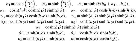 \begin{equation} \begin{array}{c} \sigma _1 = \cosh \left ( \frac {h_0 k}{2} \right ), \quad \sigma _2 = \sinh \left ( \frac {h_0 k}{2} \right ), \quad \sigma _3 = \sinh \left ( k(h_0 + h_1 + h_2) \right ), \\[2pt] \alpha _1 = \cosh (h_0 k) \cosh (h_1 k) \sinh (h_2 k), \quad \alpha _2 = \cosh (h_0 k) \cosh (h_2 k) \sinh (h_1 k), \\[2pt] \alpha _3 = \cosh (h_1 k) \cosh (h_2 k) \sinh (h_0 k), \quad \alpha _4 = \sinh (h_0 k) \sinh (h_1 k) \sinh (h_2 k), \\[2pt] \alpha _5 = \cosh (h_0 k) \sinh (h_1 k) \sinh (h_2 k), \quad \alpha _6 = \cosh (h_2 k) \sinh (h_0 k) \sinh (h_1 k), \\[2pt] \alpha _7 = \cosh (h_1 k) \sinh (h_0 k) \sinh (h_2 k),\\[2pt] \beta _1 = \sinh (h_1 k) \, \sinh (h_2 k), \quad \beta _2 = \cosh (h_1 k) \, \sinh (h_2 k), \\[2pt] \beta _3 = \cosh (h_2 k) \, \sinh (h_1 k), \quad \beta _4 = \cosh (h_1 k) \, \cosh (h_2 k). \end{array} \end{equation}
The lower deck expresses all composite terms that couple the middle-deck hyperbolic functions with velocities and gravitational accelerations. This layer systematically simplifies and organises the structure of
 $b_n$
$b_n$
 \begin{align} &\gamma _1 = -\frac {g_1(\alpha _5 + \alpha _6)}{k}, \quad \gamma _2 = -\frac {g_2(\alpha _5 + \alpha _7)}{k}, \quad \gamma _3 = \frac {\big(1 - 2 \sigma _1^2\big)\beta _1(g_1 + g_2)}{k}, \nonumber \\ & \nonumber \gamma _4 = -\frac {2 g_1 \beta _3 \sigma _1 \sigma _2}{k}, \quad \gamma _5 = -\frac {2 g_2 \beta _2 \sigma _1 \sigma _2}{k}, \quad \gamma _6 = \frac {2 g_1 g_2 \sigma _1 \beta _1 \sigma _2}{k^2}, \\ & \gamma _7 = 2\big(u_0 u_1^2 + u_0^2 u_1\big)\beta _2 + 2\big(u_0 u_2^2 + u_0^2 u_2\big)\beta _3 + \frac {2 u_0 \beta _1(g_1 + g_2)}{k}, \\ & \nonumber \gamma _8 = 8 u_0^3 \beta _1 + 4 u_1 u_2(u_1 + u_2) \beta _4 - u_2 \frac {4 g_1 \beta _3}{k} - u_1 \frac {4 g_2 \beta _2}{k}, \\ & \nonumber\gamma _9 = \big(1 - 2 \sigma _1^2\big)\big(u_1^2 \beta _2 - u_2^2 \beta _3\big). \end{align}
A.2. Dispersion relation
The dispersion relation for the small tilt angle such that
 $\sin {\theta } \ll \cos {\theta }$
can be expressed in the form
$\sin {\theta } \ll \cos {\theta }$
can be expressed in the form
 \begin{equation} \sum _{n=0}^{4} b_n(\boldsymbol{q},k) c^n = 0, \end{equation}
where the wavenumber-dependent coefficients
 $b_n$
are given in Appendix A.1 and the analytical solution to (A10) is obtained by replacing
$b_n$
are given in Appendix A.1 and the analytical solution to (A10) is obtained by replacing
 $a_n$
with
$a_n$
with
 $b_n$
in (3.9) whose solution is given in (3.12). Note that the two solutions
$b_n$
in (3.9) whose solution is given in (3.12). Note that the two solutions
 $c_{1,2}$
(the first and second root of (A10)) are the speed of linear waves on the upper interface while the two solutions
$c_{1,2}$
(the first and second root of (A10)) are the speed of linear waves on the upper interface while the two solutions
 $c_{3,4}$
(the third and fourth root of (A10)) are those on the lower interface. In the long-wave limit where
$c_{3,4}$
(the third and fourth root of (A10)) are those on the lower interface. In the long-wave limit where
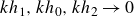 $kh_1, kh_0, kh_2 \rightarrow 0$
, we find that
$kh_1, kh_0, kh_2 \rightarrow 0$
, we find that
 $b_i \rightarrow k a_i \ (i=0, \ldots ,3)$
and that
$b_i \rightarrow k a_i \ (i=0, \ldots ,3)$
and that
 \begin{equation} c_i(k) \longrightarrow \lambda _i \quad \forall i \in \{1,2,3,4\} \quad \text{when} \ k\ll 1. \end{equation}
Therefore,
 $c_1, c_2, c_3$
and
$c_1, c_2, c_3$
and
 $c_4$
individually converge to
$c_4$
individually converge to
 $\lambda _1, \lambda _2, \lambda _3$
and
$\lambda _1, \lambda _2, \lambda _3$
and
 $\lambda _4$
in the long-wave limit. The characteristics are thus the phase speed of the linear long waves of small amplitude disturbing individual interfaces. Consequently, the imaginary part of the characteristics
$\lambda _4$
in the long-wave limit. The characteristics are thus the phase speed of the linear long waves of small amplitude disturbing individual interfaces. Consequently, the imaginary part of the characteristics
 $\lambda ^I$
of the three-layer flow also describes the potential growth (
$\lambda ^I$
of the three-layer flow also describes the potential growth (
 $\lambda ^I \gt 0$
), decay (
$\lambda ^I \gt 0$
), decay (
 $\lambda ^I \lt 0$
) or neutral state (
$\lambda ^I \lt 0$
) or neutral state (
 $\lambda ^I = 0$
) of these linear long waves on each interface.
$\lambda ^I = 0$
) of these linear long waves on each interface.
Although we neglected horizontal buoyancy forcing in the three-layer dispersion relation, it is noteworthy to comment that in the proximity of the critical layer this forcing dominates and shapes the structure of the unstable modes. This influence is attributed to the vertical derivative present on the right-hand side of (A2), leading to the appearance of
 $(\mathcal{U}-c)^{-2}$
terms, particularly evident in the long-wave limits (owing to the
$(\mathcal{U}-c)^{-2}$
terms, particularly evident in the long-wave limits (owing to the
 $1/k$
prefactor). In future work we will further investigate the properties of the solution to (A2) for various wavenumbers near the critical layers.
$1/k$
prefactor). In future work we will further investigate the properties of the solution to (A2) for various wavenumbers near the critical layers.
A.3. Pure exchange flow with stagnant middle layer
In the limit
 $u_0 = 0$
,
$u_0 = 0$
,
 $u_2 = -u_1$
,
$u_2 = -u_1$
,
 $h_2 = h_1$
and
$h_2 = h_1$
and
 $g_2 = g_1$
, corresponding to a symmetric exchange flow with a stagnant middle layer, the dispersion relation coefficients simplify to
$g_2 = g_1$
, corresponding to a symmetric exchange flow with a stagnant middle layer, the dispersion relation coefficients simplify to
 \begin{align} b_4 &= \sinh \!\left (k(h_0 + 2 h_1)\right ), \quad b_3 = 0, \quad b_1 = 0, \nonumber \\ b_2 &= \frac {2}{k} \big[ g_1 \sinh (h_1 k) \sinh (k(h_0 + h_1)) - k u_1^2 \sinh (k(h_0 - h_1)) \cosh (h_1 k) \big ], \\ b_0 &= \frac {2}{k} \big[ g_1 u_1^2 \sinh (2 h_1 k) + k \big ( g_1^2 \sinh ^2(h_1 k) + u_1^4 \cosh ^2(h_1 k) \big ) \big] \cosh \left ( \frac {h_0 k}{2} \right ) \sinh \left ( \frac {h_0 k}{2} \right ). \nonumber\end{align}
For long waves (
 $k \ll 1$
), the phase speed converges to the analytical expression given in (3.15), becoming effectively independent of
$k \ll 1$
), the phase speed converges to the analytical expression given in (3.15), becoming effectively independent of
 $k$
and, hence, non-dispersive. In this regime, the numerically computed branches
$k$
and, hence, non-dispersive. In this regime, the numerically computed branches
 $\lambda _{1}^I$
and
$\lambda _{1}^I$
and
 $\lambda _{4}^I$
, as illustrated in figure 5, are indistinguishable from long-wave speeds
$\lambda _{4}^I$
, as illustrated in figure 5, are indistinguishable from long-wave speeds
 $c_{1}^I$
and
$c_{1}^I$
and
 $c_{4}^I$
, where
$c_{4}^I$
, where
 $k = 0.001$
is chosen to represent the long-wave limit.
$k = 0.001$
is chosen to represent the long-wave limit.
A.4. Application to the data
The growth rate of the linear waves on the upper interface
 $c_2^I$
and the growth rate of the linear waves on the lower interface
$c_2^I$
and the growth rate of the linear waves on the lower interface
 $c_4^I$
are shown in figure 17(a,b) for the TW case (left column) and the I case (right column) at a representative time of
$c_4^I$
are shown in figure 17(a,b) for the TW case (left column) and the I case (right column) at a representative time of
 $t=180$
. The fastest growth in the upper (lower) interfacial wave in the TW case occurs in the region where
$t=180$
. The fastest growth in the upper (lower) interfacial wave in the TW case occurs in the region where
 $x \leqslant -15$
(
$x \leqslant -15$
(
 $x \geqslant 15$
). In the I case, although both upper and lower interfacial waves are unstable almost everywhere inside the duct, the
$x \geqslant 15$
). In the I case, although both upper and lower interfacial waves are unstable almost everywhere inside the duct, the
 $x \geqslant 15$
and
$x \geqslant 15$
and
 $x \leqslant -15$
regions exhibit the fastest growth rates. In both cases, both long waves (
$x \leqslant -15$
regions exhibit the fastest growth rates. In both cases, both long waves (
 $k \ll 1$
) and short waves (
$k \ll 1$
) and short waves (
 $k \gg 1$
) are unstable. The range of wavenumbers with the fastest growth rate is
$k \gg 1$
) are unstable. The range of wavenumbers with the fastest growth rate is
 $0.1 \leqslant k \leqslant 2$
, with the peak around
$0.1 \leqslant k \leqslant 2$
, with the peak around
 $k \approx 1$
. Consistently, many previous linear studies showed saturation in the growth rate of short waves for
$k \approx 1$
. Consistently, many previous linear studies showed saturation in the growth rate of short waves for
 $k=1.5$
, leading to Kelvin–Helmholtz and Holmboe instabilities, depending on the thickness of the density interface (Smyth & Peltier Reference Smyth and Peltier1991; Lefauve et al. Reference Lefauve, Partridge, Zhou, Dalziel, Caulfield and Linden2018; Ducimetière et al. Reference Ducimetière, Gallaire, Lefauve and Caulfield2021).
$k=1.5$
, leading to Kelvin–Helmholtz and Holmboe instabilities, depending on the thickness of the density interface (Smyth & Peltier Reference Smyth and Peltier1991; Lefauve et al. Reference Lefauve, Partridge, Zhou, Dalziel, Caulfield and Linden2018; Ducimetière et al. Reference Ducimetière, Gallaire, Lefauve and Caulfield2021).
In figure 17(c) the product
 $c_2^I c_4^I$
is shown to highlight the regions in the flow with simultaneous amplification of the growth rates of the interfacial waves. The product
$c_2^I c_4^I$
is shown to highlight the regions in the flow with simultaneous amplification of the growth rates of the interfacial waves. The product
 $c_2^I c_4^I$
is largest for medium and long waves (
$c_2^I c_4^I$
is largest for medium and long waves (
 $k \lt 1$
) in all cases. In the I case, this simultaneous amplification occurs over a more extended region inside the duct compared with the TW case, where it is more localised near the centre at
$k \lt 1$
) in all cases. In the I case, this simultaneous amplification occurs over a more extended region inside the duct compared with the TW case, where it is more localised near the centre at
 $x=0$
, consistent with the large values of TKE in figure 9 at the duct centre.
$x=0$
, consistent with the large values of TKE in figure 9 at the duct centre.
Dispersion relation of the linear interfacial waves for the TW case (left column) and the I case (right column) at
 $t=180$
. Based on the analytical solution given in (A10) and (A9), we show (a) the lower interface growth rate
$t=180$
. Based on the analytical solution given in (A10) and (A9), we show (a) the lower interface growth rate
 $c_2^I$
, (b) the upper interface growth rate
$c_2^I$
, (b) the upper interface growth rate
 $c_4^I$
and (c) the amplification of the growth rate
$c_4^I$
and (c) the amplification of the growth rate
 $c_2^I c_4^I$
.
$c_2^I c_4^I$
.
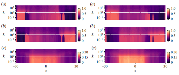
The dispersivity
 $d_g$
of the I case at various
$d_g$
of the I case at various
 $x$
locations are shown in figure 18(a,b) (active stage) and figure 18(c,d) (quiet stage). The
$x$
locations are shown in figure 18(a,b) (active stage) and figure 18(c,d) (quiet stage). The
 $d_g$
plot for the SW and TW cases is overall similar to the quiet stage of the I case and is not shown here for brevity. We observe that
$d_g$
plot for the SW and TW cases is overall similar to the quiet stage of the I case and is not shown here for brevity. We observe that
 $d_g \rightarrow 0$
in the long-wave limit (
$d_g \rightarrow 0$
in the long-wave limit (
 $k \rightarrow 0$
) as expected. The most dispersive waves are short, with
$k \rightarrow 0$
) as expected. The most dispersive waves are short, with
 $1 \leqslant k \leqslant 2$
for all
$1 \leqslant k \leqslant 2$
for all
 $x$
and
$x$
and
 $t$
. This range of wavenumbers also corresponds to the fastest growth in the amplitude of the linear waves, as shown in the right columns of figure 17(a,b) for these short waves. In the quiet stage, the dispersivity of the waves is almost independent of
$t$
. This range of wavenumbers also corresponds to the fastest growth in the amplitude of the linear waves, as shown in the right columns of figure 17(a,b) for these short waves. In the quiet stage, the dispersivity of the waves is almost independent of
 $x$
away from the inlet and outlet (figure 18
c,d). In the active stage, however, the spatial variation in
$x$
away from the inlet and outlet (figure 18
c,d). In the active stage, however, the spatial variation in
 $d_g$
is more pronounced.
$d_g$
is more pronounced.
Dispersivity values
 $\lvert {d_g} \rvert$
of disturbance waves in case I at various
$\lvert {d_g} \rvert$
of disturbance waves in case I at various
 $x$
locations at
$x$
locations at
 $t=110$
during the active stage (a,b) and at
$t=110$
during the active stage (a,b) and at
 $t=180$
in the quiet stage (c,d). In panels (a,c) the
$t=180$
in the quiet stage (c,d). In panels (a,c) the
 $\lvert {d_g} \rvert$
of the upper interfacial waves is presented, while panels (c,d) show the dispersivity of the lower interfacial waves.
$\lvert {d_g} \rvert$
of the upper interfacial waves is presented, while panels (c,d) show the dispersivity of the lower interfacial waves.
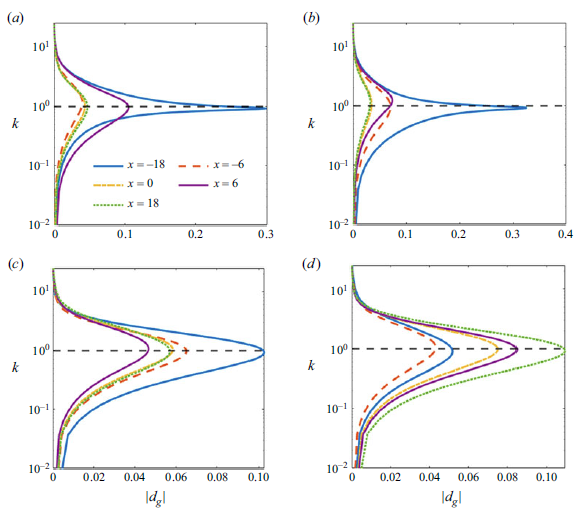
Appendix B. Spectral gap and long–long-wave resonance
The concept of the spectral gap is well established in matrix perturbation theory (see, for example, Stewart Reference Stewart1975; Elsner & Sun Reference Elsner and Sun1982). In this section we review this concept for completeness and apply it within the context of a three-layer system and the resonance between long waves in the subsystems defined in the building-block (matrix) decomposition of (4.1).
B.1. Three-layer system decomposition and the spectral gap
We consider a real matrix pair, denoted
 $\unicode{x1D648}$
, with dimensions
$\unicode{x1D648}$
, with dimensions
 $6 \times 12$
, associated with a three-layer system. Using figure 19, we represent its characteristics,
$6 \times 12$
, associated with a three-layer system. Using figure 19, we represent its characteristics,
 $\lambda (\unicode{x1D648}{\kern2pt}) \in \mathbb{C}$
, which consist of real and imaginary components, as
$\lambda (\unicode{x1D648}{\kern2pt}) \in \mathbb{C}$
, which consist of real and imaginary components, as
 \begin{eqnarray} \lambda (\unicode{x1D648}{\kern2pt}) = \lambda ^R(\unicode{x1D648}{\kern2pt}) + i \lambda ^I(\unicode{x1D648}{\kern2pt}) = (\lambda ^R(\unicode{x1D648}{\kern2pt}), \lambda ^I(\unicode{x1D648}{\kern2pt}), 0)=\boldsymbol{P_c}. \end{eqnarray}
Next, we apply stereographic projection to map these characteristics onto the unit sphere. Stereographic projection is a standard technique for mapping points from a plane – in this case, the complex plane of eigenvalues – onto a (Riemann) sphere. This projection enables a geometrically meaningful analysis of the matrix’s spectral properties, as each point on the sphere corresponds to a pair of real and imaginary components from the complex plane, revealing insights into the eigenvalue structure. This approach is also geometrically instructive for examining
 $\lambda (\unicode{x1D648}{\kern2pt})$
against a second matrix pair with strictly real characteristics, which vary within the range
$\lambda (\unicode{x1D648}{\kern2pt})$
against a second matrix pair with strictly real characteristics, which vary within the range
 $[-1,1]$
, as is the case, for example, for
$[-1,1]$
, as is the case, for example, for
 $\lambda (\unicode{x1D655}{\kern2pt})$
.
$\lambda (\unicode{x1D655}{\kern2pt})$
.
We define a point on the sphere as
 $\boldsymbol{P} = (\lambda ^R_1, \lambda ^I_1, \lambda ({\unicode{x1D655}_1}{\kern2pt}))$
that is the stereographic projection of
$\boldsymbol{P} = (\lambda ^R_1, \lambda ^I_1, \lambda ({\unicode{x1D655}_1}{\kern2pt}))$
that is the stereographic projection of
 $\boldsymbol{P_c}$
, where the unit sphere is constructed such that
$\boldsymbol{P_c}$
, where the unit sphere is constructed such that
 \begin{equation} \big (\lambda ^R_1\big)^2 + \big(\lambda ^I_1\big)^2 + \lambda ({\unicode{x1D655}_1}{\kern2pt})^2 = 1. \end{equation}
The north pole of the sphere is denoted by
 $\boldsymbol{N} = (0, 0, 1)$
, and the line connecting
$\boldsymbol{N} = (0, 0, 1)$
, and the line connecting
 $\boldsymbol{N}$
to the point
$\boldsymbol{N}$
to the point
 $\lambda (\unicode{x1D648}{\kern2pt})$
on the complex plane is given by the parametric equation
$\lambda (\unicode{x1D648}{\kern2pt})$
on the complex plane is given by the parametric equation
 \begin{align} \big(\lambda ^R_1, \lambda ^I_1, \lambda ({\unicode{x1D655}_1}{\kern2pt})\big) &= (1-s)\lambda (\unicode{x1D648}{\kern2pt}) + s\boldsymbol{N} \nonumber \\ &= ((1-s)\lambda ^R(\unicode{x1D648}{\kern2pt}), (1-s)\lambda ^I(\unicode{x1D648}{\kern2pt}), s), \quad \forall s \in \mathbb{R} - \{1\}. \end{align}
Here,
 $s$
is a parameter that controls the position along the line between the point
$s$
is a parameter that controls the position along the line between the point
 $\lambda (\unicode{x1D648}{\kern2pt})$
and the north pole
$\lambda (\unicode{x1D648}{\kern2pt})$
and the north pole
 $\boldsymbol{N}$
. When
$\boldsymbol{N}$
. When
 $s = 0$
, the point is at
$s = 0$
, the point is at
 $\lambda (\unicode{x1D648}{\kern2pt})$
, and when
$\lambda (\unicode{x1D648}{\kern2pt})$
, and when
 $s$
approaches unity the point reaches the north pole
$s$
approaches unity the point reaches the north pole
 $\boldsymbol{N}$
. If one takes the magnitude of both sides of (B3) and substitutes the condition of the unit sphere, given by (B2), we relate the square of the distance between the projection point and the origin (i.e. the squared magnitude of
$\boldsymbol{N}$
. If one takes the magnitude of both sides of (B3) and substitutes the condition of the unit sphere, given by (B2), we relate the square of the distance between the projection point and the origin (i.e. the squared magnitude of
 $\lambda (\unicode{x1D648}{\kern2pt})$
in the complex plane) to the parameter
$\lambda (\unicode{x1D648}{\kern2pt})$
in the complex plane) to the parameter
 $s$
:
$s$
:
 \begin{eqnarray} {\lvert {\lambda (\unicode{x1D648}{\kern2pt})} \rvert }^2 = \big(\lambda ^R(\unicode{x1D648}{\kern2pt})\big )^2 + \big(\lambda ^I(\unicode{x1D648}{\kern2pt})\big)^2 = \frac {1+s}{1-s}. \end{eqnarray}
This result shows that the stereographic projection maps points from the complex plane onto the sphere in such a way that the distance from the origin in the complex plane,
 $\lvert {\lambda (\unicode{x1D648}{\kern2pt})} \rvert$
, is related to the projection parameter
$\lvert {\lambda (\unicode{x1D648}{\kern2pt})} \rvert$
, is related to the projection parameter
 $s$
by the formula
$s$
by the formula
 $({1+s})/({1-s})$
. This relationship provides a geometric interpretation of how the spectral characteristics of the matrix are represented on the sphere. To do so, we solve for
$({1+s})/({1-s})$
. This relationship provides a geometric interpretation of how the spectral characteristics of the matrix are represented on the sphere. To do so, we solve for
 $s$
to obtain
$s$
to obtain
 \begin{eqnarray} s = \frac {{\lvert {\lambda (\unicode{x1D648}{\kern2pt})}\rvert }^2 - 1}{{\lvert {\lambda (\unicode{x1D648}{\kern2pt})} \rvert }^2 + 1}. \end{eqnarray}
We now substitute (B5) into (B3) to express the real and imaginary components of the projection on the sphere:
 \begin{eqnarray} && \lambda ^R_1 = \frac {2 \lambda ^R(\unicode{x1D648}{\kern2pt})}{1 + {\lvert {\lambda (\unicode{x1D648}{\kern2pt})} \rvert }^2}, \quad \lambda ^I_1 = \frac {2 \lambda ^I(\unicode{x1D648}{\kern2pt})}{1 + {\lvert {\lambda (\unicode{x1D648}{\kern2pt})} \rvert }^2}, \quad \lambda ({\unicode{x1D655}_1}) = \frac {{\lvert {\lambda (\unicode{x1D648}{\kern2pt})} \rvert }^2 - 1}{{\lvert {\lambda (\unicode{x1D648}{\kern2pt})} \rvert }^2 + 1}. \qquad \end{eqnarray}
The stereographic projection allows us to map all points
 $(\lambda ^R_1, \lambda ^I_1, \lambda (\unicode{x1D655}{\kern2pt}))$
on the sphere to corresponding points in the complex plane
$(\lambda ^R_1, \lambda ^I_1, \lambda (\unicode{x1D655}{\kern2pt}))$
on the sphere to corresponding points in the complex plane
 $\mathbb{C}$
, constructed from the eigenvalues of
$\mathbb{C}$
, constructed from the eigenvalues of
 $\unicode{x1D648}$
.
$\unicode{x1D648}$
.
Next, consider another point
 $\boldsymbol{Q} = (\lambda ^R_2, \lambda ^I_2, \lambda ({\unicode{x1D655}_2}))$
on the sphere, where
$\boldsymbol{Q} = (\lambda ^R_2, \lambda ^I_2, \lambda ({\unicode{x1D655}_2}))$
on the sphere, where
 \begin{equation} \big(\lambda ^R_2\big)^2 + \big(\lambda ^I_2\big)^2 + \lambda ({\unicode{x1D655}_2})^2 = 1, \end{equation}
which connects
 $\boldsymbol{N}$
to
$\boldsymbol{N}$
to
 $\lambda (\unicode{x1D648} + {\unicode{x1D648}{\kern2pt}'}{\kern2pt})$
. We can write a similar expression to relate the components of
$\lambda (\unicode{x1D648} + {\unicode{x1D648}{\kern2pt}'}{\kern2pt})$
. We can write a similar expression to relate the components of
 $\boldsymbol{Q}$
to
$\boldsymbol{Q}$
to
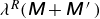 $\lambda ^R(\unicode{x1D648} + {\unicode{x1D648}{\kern2pt}'}{\kern2pt})$
and
$\lambda ^R(\unicode{x1D648} + {\unicode{x1D648}{\kern2pt}'}{\kern2pt})$
and
 $\lambda ^I(\unicode{x1D648} + {\unicode{x1D648}{\kern2pt}'}{\kern2pt})$
as
$\lambda ^I(\unicode{x1D648} + {\unicode{x1D648}{\kern2pt}'}{\kern2pt})$
as
 \begin{align} \lambda ^R_2 = \frac {2 \lambda ^R(\unicode{x1D648} + {\unicode{x1D648}{\kern2pt}'}{\kern2pt})}{1 + {\lvert {\lambda (\unicode{x1D648} + {\unicode{x1D648}{\kern2pt}'}{\kern2pt})} \rvert }^2}, \quad \lambda ^I_2 = \frac {2 \lambda ^I(\unicode{x1D648} + {\unicode{x1D648}{\kern2pt}'}{\kern2pt})}{1 + {\lvert {\lambda (\unicode{x1D648} + {\unicode{x1D648}{\kern2pt}'}{\kern2pt})} \rvert }^2}, \quad \lambda ({\unicode{x1D655}_2}) = \frac {{\lvert {\lambda (\unicode{x1D648} + {\unicode{x1D648}{\kern2pt}'}{\kern2pt})} \rvert }^2 - 1}{{\lvert {\lambda (\unicode{x1D648} + {\unicode{x1D648}{\kern2pt}'}{\kern2pt})} \rvert }^2 + 1}. \qquad \end{align}
The Euclidean distance
 $\lvert {\boldsymbol{PQ}} \rvert$
between
$\lvert {\boldsymbol{PQ}} \rvert$
between
 $\boldsymbol{P}$
and
$\boldsymbol{P}$
and
 $\boldsymbol{Q}$
is
$\boldsymbol{Q}$
is
 \begin{eqnarray} {\lvert {\boldsymbol{PQ}} \rvert } &=& \sqrt {\left (\lambda ^R_1 - \lambda ^R_2\right )^2 + \left (\lambda ^I_1 - \lambda ^I_2\right )^2 + \left (\lambda ({\unicode{x1D655}_1}) - \lambda ({\unicode{x1D655}_2})\right )^2} \nonumber \\ &=& \sqrt {2 - 2\left (\lambda ^R_1\lambda ^R_2 + \lambda ^I_1\lambda ^I_2 + \lambda ({\unicode{x1D655}_1})\lambda ({\unicode{x1D655}_2}) \right )} \end{eqnarray}
due to the constraints (B2) and (B7), noting that the term inside the bracket yields
 $\boldsymbol{P} \cdot \boldsymbol{Q}$
that is equal to the cosine of the angle between the two vectors connecting
$\boldsymbol{P} \cdot \boldsymbol{Q}$
that is equal to the cosine of the angle between the two vectors connecting
 $\boldsymbol{P}$
and
$\boldsymbol{P}$
and
 $\boldsymbol{Q}$
to the origin. Using the expressions from (B6) and (B8), we conclude that
$\boldsymbol{Q}$
to the origin. Using the expressions from (B6) and (B8), we conclude that
 \begin{equation} \lambda ^R_1\lambda ^R_2 + \lambda ^I_1\lambda ^I_2 + \lambda ({\unicode{x1D655}_1})\lambda ({\unicode{x1D655}_2}) = 1 - \frac {2 {\lvert {\lambda (\unicode{x1D648} + {\unicode{x1D648}{\kern2pt}'}{\kern2pt}) - \lambda (\unicode{x1D648}{\kern2pt})} \rvert }^2}{\big( {\lvert {\lambda (\unicode{x1D648} + {\unicode{x1D648}{\kern2pt}'}{\kern2pt})} \rvert }^2 + 1 \big) \big( {\lvert {\lambda (\unicode{x1D648}{\kern2pt})} \rvert }^2 + 1 \big)}, \end{equation}
which leads to the final form of the Euclidean distance:
 \begin{equation} {\lvert {\boldsymbol{PQ}} \rvert } = \frac { {\lvert {\lambda (\unicode{x1D648} + {\unicode{x1D648}{\kern2pt}'}{\kern2pt}) - \lambda (\unicode{x1D648}{\kern2pt})} \rvert }}{\sqrt {{\lvert {\lambda (\unicode{x1D648} + {\unicode{x1D648}{\kern2pt}'}{\kern2pt})} \rvert }^2 + 1} \sqrt {{\lvert {\lambda (\unicode{x1D648}{\kern2pt})} \rvert }^2 + 1}}. \end{equation}
This expression represents the distance between two arbitrary points on the Riemann sphere based on the spectra of two arbitrary matrices. The matrices
 $\unicode{x1D648}$
and
$\unicode{x1D648}$
and
 $\unicode{x1D648} + {\unicode{x1D648}{\kern2pt}'}$
are square matrix pairs of size
$\unicode{x1D648} + {\unicode{x1D648}{\kern2pt}'}$
are square matrix pairs of size
 $6 \times 12$
, each having six eigenvalues. Based on (B11), we can construct the spectral variation matrix as
$6 \times 12$
, each having six eigenvalues. Based on (B11), we can construct the spectral variation matrix as
 \begin{eqnarray} d_{jk}(\unicode{x1D648} + {\unicode{x1D648}{\kern2pt}'}, \unicode{x1D648}{\kern2pt}) = \frac {\lambda _j(\unicode{x1D648} + {\unicode{x1D648}{\kern2pt}'}{\kern2pt}) - \lambda _k(\unicode{x1D648}{\kern2pt})}{\sqrt {{\lvert {\lambda _j(\unicode{x1D648} + {\unicode{x1D648}{\kern2pt}'}{\kern2pt})} \rvert }^2 + 1} \sqrt {{\lvert {\lambda _k(\unicode{x1D648}{\kern2pt})}\rvert }^2 + 1}}, \quad 1 \leqslant j, k \leqslant 4, \end{eqnarray}
which measures variation among all characteristics of
 $\unicode{x1D648}$
and
$\unicode{x1D648}$
and
 $\unicode{x1D648} + {\unicode{x1D648}{\kern2pt}'}$
. The spectral variation between
$\unicode{x1D648} + {\unicode{x1D648}{\kern2pt}'}$
. The spectral variation between
 $\unicode{x1D648}$
and
$\unicode{x1D648}$
and
 $\unicode{x1D648} + {\unicode{x1D648}{\kern2pt}'}$
is also illustrated in figure 19 by the magnitude of the the vector
$\unicode{x1D648} + {\unicode{x1D648}{\kern2pt}'}$
is also illustrated in figure 19 by the magnitude of the the vector
 $\boldsymbol{Q}\boldsymbol{P}$
as the back projection of
$\boldsymbol{Q}\boldsymbol{P}$
as the back projection of
 $\boldsymbol{Q_c}\boldsymbol{P_c}$
onto the unit sphere, encompassing
$\boldsymbol{Q_c}\boldsymbol{P_c}$
onto the unit sphere, encompassing
 $-1 \leqslant \lambda (\boldsymbol{\zeta }) \leqslant 1$
. For each row in
$-1 \leqslant \lambda (\boldsymbol{\zeta }) \leqslant 1$
. For each row in
 $d_{jk}$
, we search for the
$d_{jk}$
, we search for the
 $k$
that results in the minimum column-wise values for
$k$
that results in the minimum column-wise values for
 $\mathcal{D}_j = {\min}\, \{{\lvert {d_{j1}}\rvert }, {\lvert {d_{j2}}\rvert }, {\lvert {d_{j3}} \rvert }, {\lvert {d_{j4}} \rvert }\}$
to construct a vector from the columns of
$\mathcal{D}_j = {\min}\, \{{\lvert {d_{j1}}\rvert }, {\lvert {d_{j2}}\rvert }, {\lvert {d_{j3}} \rvert }, {\lvert {d_{j4}} \rvert }\}$
to construct a vector from the columns of
 $d_{jk}$
that yields the least spectral variation in the
$d_{jk}$
that yields the least spectral variation in the
 $j$
th row. The spectral gap is then the infinity norm
$j$
th row. The spectral gap is then the infinity norm
 ${\lVert {\mathcal{D}}\rVert }_\infty$
. Collectively, the spectral gap is computed as
${\lVert {\mathcal{D}}\rVert }_\infty$
. Collectively, the spectral gap is computed as
 \begin{eqnarray} S_{\unicode{x1D648}}({\unicode{x1D648}{\kern2pt}'}{\kern2pt}) \equiv \max _j\, \, \min _k \ {\lvert {d_{jk} (\unicode{x1D648} + {\unicode{x1D648}{\kern2pt}'}, \unicode{x1D648}{\kern2pt})} \rvert }, \quad 1 \leqslant j, k \leqslant 4, \end{eqnarray}
which is consistent with the definition of Stewart (Reference Stewart1975) and Elsner & Sun (Reference Elsner and Sun1982).
B.2. Long-wave resonance indicator
Let us now substitute the pairs
 $\unicode{x1D648}$
and
$\unicode{x1D648}$
and
 $\unicode{x1D648} + {\unicode{x1D648}{\kern2pt}'}$
with
$\unicode{x1D648} + {\unicode{x1D648}{\kern2pt}'}$
with
 $\unicode{x1D652}$
and
$\unicode{x1D652}$
and
 $\unicode{x1D655}$
, representing the isolated upper and middle layer system defined in (4.5). Using (B13), the quantity
$\unicode{x1D655}$
, representing the isolated upper and middle layer system defined in (4.5). Using (B13), the quantity
 $S_{\unicode{x1D655}}(\unicode{x1D652}{\kern2pt})$
measures the spectral gap between
$S_{\unicode{x1D655}}(\unicode{x1D652}{\kern2pt})$
measures the spectral gap between
 $\unicode{x1D652}$
and
$\unicode{x1D652}$
and
 $\unicode{x1D655}$
. Similarly,
$\unicode{x1D655}$
. Similarly,
 $S_{\unicode{x1D655}}(\unicode{x1D654}{\kern2pt})$
measures the spectral gap between
$S_{\unicode{x1D655}}(\unicode{x1D654}{\kern2pt})$
measures the spectral gap between
 $\unicode{x1D654}$
the isolated lower layer and
$\unicode{x1D654}$
the isolated lower layer and
 $\unicode{x1D655}$
the isolated middle layer.
$\unicode{x1D655}$
the isolated middle layer.
Spectral variation between two matrix pairs,
 $\unicode{x1D648}$
and
$\unicode{x1D648}$
and
 $\unicode{x1D648} + {\unicode{x1D648}{\kern2pt}'}$
, measured by
$\unicode{x1D648} + {\unicode{x1D648}{\kern2pt}'}$
, measured by
 $\boldsymbol{Q}\boldsymbol{P}$
, the back projection of
$\boldsymbol{Q}\boldsymbol{P}$
, the back projection of
 $\boldsymbol{Q_c}\boldsymbol{P_c}$
onto the unit sphere that encompasses the spectrum of a third matrix pair,
$\boldsymbol{Q_c}\boldsymbol{P_c}$
onto the unit sphere that encompasses the spectrum of a third matrix pair,
 $\boldsymbol{\zeta }$
, whose eigenvalues satisfy
$\boldsymbol{\zeta }$
, whose eigenvalues satisfy
 $\lambda (\boldsymbol{\zeta }) \in [-1,1]$
. The north pole on the unit sphere is denoted by
$\lambda (\boldsymbol{\zeta }) \in [-1,1]$
. The north pole on the unit sphere is denoted by
 $\boldsymbol{N} = (0,0,1)$
, and
$\boldsymbol{N} = (0,0,1)$
, and
 $\boldsymbol{Q_c}\boldsymbol{P_c}$
represents the stereographic projection of
$\boldsymbol{Q_c}\boldsymbol{P_c}$
represents the stereographic projection of
 $\boldsymbol{Q}\boldsymbol{P}$
. The spectral gap,
$\boldsymbol{Q}\boldsymbol{P}$
. The spectral gap,
 $S_{\unicode{x1D648}}({\unicode{x1D648}{\kern2pt}'}) = {\lvert {\boldsymbol{Q}\boldsymbol{P}}\rvert }/2$
, quantifies the magnitude of spectral variation between
$S_{\unicode{x1D648}}({\unicode{x1D648}{\kern2pt}'}) = {\lvert {\boldsymbol{Q}\boldsymbol{P}}\rvert }/2$
, quantifies the magnitude of spectral variation between
 $\unicode{x1D648}$
and
$\unicode{x1D648}$
and
 $\unicode{x1D648} + {\unicode{x1D648}{\kern2pt}'}$
. The resonance condition requires
$\unicode{x1D648} + {\unicode{x1D648}{\kern2pt}'}$
. The resonance condition requires
 $P^* = Q^*$
.
$P^* = Q^*$
.
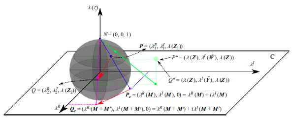
To quantify resonant interactions in DNS data, we measure the relative spectral gap between perturbed upper and lower layers with respect to the isolated middle layer as
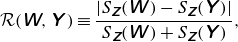 \begin{eqnarray} \mathcal{R}(\unicode{x1D652},\unicode{x1D654}{\kern2pt})\equiv \frac {{\lvert {S_{\unicode{x1D655}}(\unicode{x1D652}{\kern2pt})-S_{{\unicode{x1D655}}}(\unicode{x1D654}{\kern2pt})}\rvert }}{S_{\unicode{x1D655}}(\unicode{x1D652}{\kern2pt})+S_{\unicode{x1D655}}(\unicode{x1D654}{\kern2pt})}, \end{eqnarray}
which yields
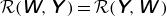 $\mathcal{R}(\unicode{x1D652},\unicode{x1D654}{\kern2pt})=\mathcal{R}(\unicode{x1D654},\unicode{x1D652}{\kern2pt})$
, whereas
$\mathcal{R}(\unicode{x1D652},\unicode{x1D654}{\kern2pt})=\mathcal{R}(\unicode{x1D654},\unicode{x1D652}{\kern2pt})$
, whereas
 $S_{\unicode{x1D655}}(\unicode{x1D652}{\kern2pt}) \neq S_{\unicode{x1D652}}(\unicode{x1D655}{\kern2pt}) \neq S_{{\unicode{x1D655}}}(\unicode{x1D654}{\kern2pt})$
in general. From the definition of
$S_{\unicode{x1D655}}(\unicode{x1D652}{\kern2pt}) \neq S_{\unicode{x1D652}}(\unicode{x1D655}{\kern2pt}) \neq S_{{\unicode{x1D655}}}(\unicode{x1D654}{\kern2pt})$
in general. From the definition of
 $\mathcal{R}(\unicode{x1D652},\unicode{x1D654}{\kern2pt})$
in (B14), and employing (B13) to compute
$\mathcal{R}(\unicode{x1D652},\unicode{x1D654}{\kern2pt})$
in (B14), and employing (B13) to compute
 $S_{\unicode{x1D655}}(\unicode{x1D652}{\kern2pt})$
and
$S_{\unicode{x1D655}}(\unicode{x1D652}{\kern2pt})$
and
 $S_{\unicode{x1D655}}(\unicode{x1D654}{\kern2pt})$
while utilising the fact that
$S_{\unicode{x1D655}}(\unicode{x1D654}{\kern2pt})$
while utilising the fact that
 $\lambda (\unicode{x1D655}{\kern2pt})$
has only one real value, we deduce (4.8).
$\lambda (\unicode{x1D655}{\kern2pt})$
has only one real value, we deduce (4.8).
Appendix C. Instantaneous profiles of TKE,
 $\mathcal{R}$
and
$\mathcal{S}$
$\mathcal{R}$
and
$\mathcal{S}$


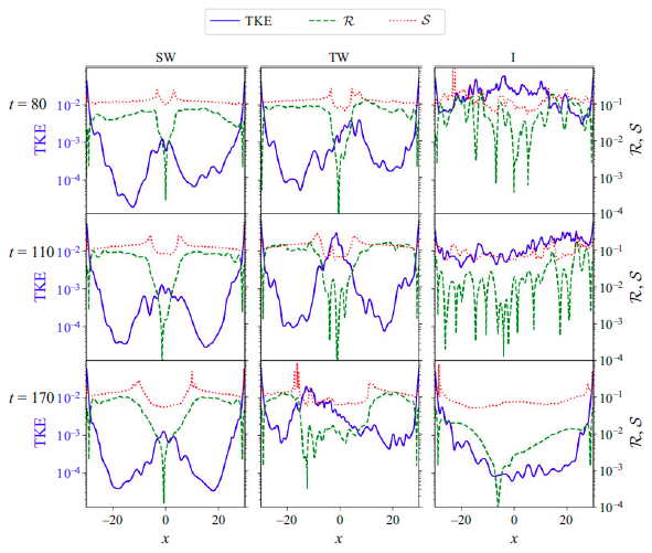
Figure 20 presents the instantaneous profiles of the TKE, averaged over the duct cross-section, alongside the long–long wave resonance indicator
 $\mathcal{R}$
and long–short wave resonance indicator
$\mathcal{R}$
and long–short wave resonance indicator
 $\mathcal{S}$
at
$\mathcal{S}$
at
 $t=0$
,
$t=0$
,
 $t=110$
and
$t=110$
and
 $t=170$
for the SW, TW and I cases. Although the space–time distributions of these quantities are already shown in figures 9, 12 and 15, these profiles provide a more detailed visualisation of their distribution at specific times.
$t=170$
for the SW, TW and I cases. Although the space–time distributions of these quantities are already shown in figures 9, 12 and 15, these profiles provide a more detailed visualisation of their distribution at specific times.
For all cases,
 $\mathcal{R}$
reaches local minima near the ends of the duct, where the TKE is most pronounced. In contrast,
$\mathcal{R}$
reaches local minima near the ends of the duct, where the TKE is most pronounced. In contrast,
 $\mathcal{S}$
is not minimised at the duct ends, suggesting that long–short wave resonance does not occur there; instead, the route to turbulence stems from both long–long wave resonance and short-wave instability without significant interaction with long waves.
$\mathcal{S}$
is not minimised at the duct ends, suggesting that long–short wave resonance does not occur there; instead, the route to turbulence stems from both long–long wave resonance and short-wave instability without significant interaction with long waves.
In the wave cases, as we move towards the centre of the duct, long–short wave resonance becomes more prominent, with
 $\mathcal{S}$
reaching minimum values where small local minima of
$\mathcal{S}$
reaching minimum values where small local minima of
 $\mathcal{R}$
and strong TKE are observed. For the I case, the entire duct exhibits strong fluctuations at
$\mathcal{R}$
and strong TKE are observed. For the I case, the entire duct exhibits strong fluctuations at
 $t=80$
and
$t=80$
and
 $t=110$
due to intense turbulence, indicating that the transition has likely occurred, making further discussion of hydraulic transition less relevant. However, at
$t=110$
due to intense turbulence, indicating that the transition has likely occurred, making further discussion of hydraulic transition less relevant. However, at
 $t=170$
, fluctuations are significantly reduced due to the intermittent nature of this case. Here,
$t=170$
, fluctuations are significantly reduced due to the intermittent nature of this case. Here,
 $\mathcal{R}$
shows minimum values near the duct centre, and
$\mathcal{R}$
shows minimum values near the duct centre, and
 $\mathcal{S}$
is reduced in a pattern similar to that observed in the wave case. This suggests that both long–long and long–short wave resonances may also occur during the quiet phase of the intermittent case, potentially leading to stronger turbulence at later times.
$\mathcal{S}$
is reduced in a pattern similar to that observed in the wave case. This suggests that both long–long and long–short wave resonances may also occur during the quiet phase of the intermittent case, potentially leading to stronger turbulence at later times.
Appendix D. Information propagation in the presence of complex characteristics
When
 $ \lambda$
is real, the coordinate transformation
$ \lambda$
is real, the coordinate transformation
 $ \xi _{\pm } = t \pm x/\lambda$
identifies characteristic curves along which combinations of flow variables are conserved in the homogeneous inviscid limit. We now explore the implications of this transformation when
$ \xi _{\pm } = t \pm x/\lambda$
identifies characteristic curves along which combinations of flow variables are conserved in the homogeneous inviscid limit. We now explore the implications of this transformation when
 $ \lambda \in \mathbb{C}$
, and the system is extended into the complex plane using the transformation
$ \lambda \in \mathbb{C}$
, and the system is extended into the complex plane using the transformation
 \begin{eqnarray} \widetilde {x} = x(1 + \epsilon i), \quad \widetilde {t} = t(1 + \epsilon i), \end{eqnarray}
where
 $\epsilon \ll 1$
is a small parameter and
$\epsilon \ll 1$
is a small parameter and
 $i$
is the imaginary unit. Using the chain rule we relate spatiotemporal variation of the state vector
$i$
is the imaginary unit. Using the chain rule we relate spatiotemporal variation of the state vector
 $\boldsymbol{q}(x,t)$
and the transformed state vector
$\boldsymbol{q}(x,t)$
and the transformed state vector
 $\boldsymbol{q}(\widetilde {x}, \widetilde {t})$
directly, i.e.
$\boldsymbol{q}(\widetilde {x}, \widetilde {t})$
directly, i.e.
 \begin{eqnarray} \frac {\partial \boldsymbol{q}(x, t)}{\partial x} = \mathrm{Re}\! \left ((1 + \epsilon i) \frac {\partial \boldsymbol{q}(\widetilde {x}, \widetilde {t})}{\partial \widetilde {x}}\right ), \qquad \frac {\partial \boldsymbol{q}(x, t)}{\partial t} = \mathrm{Re}\! \left ((1 + \epsilon i) \frac {\partial \boldsymbol{q}(\widetilde {x}, \widetilde {t})}{\partial \widetilde {t}}\right ), \end{eqnarray}
to leading order. We also expand
 $ \lambda (x,t)$
in terms of
$ \lambda (x,t)$
in terms of
 $(\widetilde {x}, \widetilde {t})$
using a Taylor series expansion
$(\widetilde {x}, \widetilde {t})$
using a Taylor series expansion
 \begin{eqnarray} \lambda (x,t) = \lambda (\widetilde {x}, \widetilde {t}) - \epsilon i \left ( \widetilde {x} \frac {\partial \lambda (\widetilde {x}, \widetilde {t})}{\partial \widetilde {x}} + \widetilde {t} \frac {\partial \lambda (\widetilde {x}, \widetilde {t})}{\partial \widetilde {t}} \right ) + \mathcal{O}(\epsilon ^2). \end{eqnarray}
Substituting (D2) and (D3) into
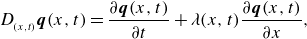 \begin{align} D_{_{(x,t)}}\boldsymbol{q}(x,t) = \frac {\partial \boldsymbol{q}(x,t)}{\partial t} + \lambda (x,t) \frac {\partial \boldsymbol{q}(x,t)}{\partial x}, \end{align}
and using (3.8), we obtain the modified equation in terms of
 $ (\widetilde {x}, \widetilde {t})$
, i.e.
$ (\widetilde {x}, \widetilde {t})$
, i.e.
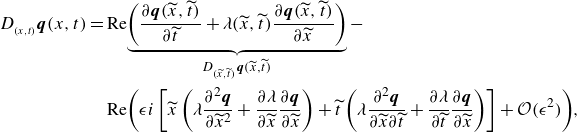 \begin{eqnarray} D_{_{(x,t)}}\boldsymbol{q}(x,t) & = & \mathrm{Re} {\underbrace {\left (\frac {\partial \boldsymbol{q}(\widetilde {x}, \widetilde {t})}{\partial \widetilde {t}} + \lambda (\widetilde {x}, \widetilde {t}) \frac {\partial \boldsymbol{q}(\widetilde {x}, \widetilde {t})}{\partial \widetilde {x}}\right )}_{D_{_{(\widetilde {x}, \widetilde {t})}}\boldsymbol{q}(\widetilde {x}, \widetilde {t})}} - \nonumber \\ &&\mathrm{Re} {\left (\epsilon i \left [ \widetilde {x} \left ( \lambda \frac {\partial ^2 \boldsymbol{q}}{\partial \widetilde {x}^2} + \frac {\partial \lambda }{\partial \widetilde {x}} \frac {\partial \boldsymbol{q}}{\partial \widetilde {x}} \right ) + \widetilde {t} \left ( \lambda \frac {\partial ^2 \boldsymbol{q}}{\partial \widetilde {x} \partial \widetilde {t}} + \frac {\partial \lambda }{\partial \widetilde {t}} \frac {\partial \boldsymbol{q}}{\partial \widetilde {x}} \right ) \right ] + \mathcal{O}(\epsilon ^2)\right )},\qquad \end{eqnarray}
assuming that
 $\boldsymbol{q}(\widetilde {x}, \widetilde {t})$
and
$\boldsymbol{q}(\widetilde {x}, \widetilde {t})$
and
 $\lambda (\widetilde {x}, \widetilde {t})$
are both analytic.
$\lambda (\widetilde {x}, \widetilde {t})$
are both analytic.
D.1. Transformation to characteristic variables
We now introduce characteristic coordinates
 \begin{eqnarray} \xi _+ = \widetilde {t} + \frac {\widetilde {x}}{\lambda (\widetilde {x}, \widetilde {t})}, \quad \xi _- = \widetilde {t} - \frac {\widetilde {x}}{\lambda (\widetilde {x}, \widetilde {t})}. \end{eqnarray}
These define complex-valued curves in space–time. The real parts of these coordinates correspond to directions of propagation in physical space, with inverse
 \begin{eqnarray} \widetilde {t} = \frac {1}{2}(\xi _+ + \xi _-), \quad \widetilde {x} = \frac {\lambda }{2}(\xi _+ - \xi _-), \end{eqnarray}
and, therefore, become complex if characteristics are complex, which justifies our change of coordinate from
 $x$
and
$x$
and
 $t$
to
$t$
to
 $\widetilde {x}$
and
$\widetilde {x}$
and
 $\widetilde {t}$
. Using the chain rule
$\widetilde {t}$
. Using the chain rule
 \begin{eqnarray} \frac {\partial }{\partial \widetilde {x}} &=& \frac {\partial \xi _\pm }{\partial \widetilde {x}} \frac {d}{{\rm d}\xi _\pm }, \quad \frac {\partial }{\partial \widetilde {t}} = \frac {\partial \xi _\pm }{\partial \widetilde {t}} \frac {d}{{\rm d}\xi _\pm }, \end{eqnarray}
with
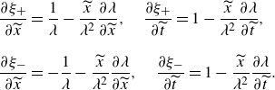 \begin{equation} \begin{aligned} \frac {\partial \xi _+}{\partial \widetilde {x}} &= \frac {1}{\lambda } - \frac {\widetilde {x}}{\lambda ^2} \frac {\partial \lambda }{\partial \widetilde {x}}, \quad \frac {\partial \xi _+}{\partial \widetilde {t}} = 1 - \frac {\widetilde {x}}{\lambda ^2} \frac {\partial \lambda }{\partial \widetilde {t}},\nonumber \\[10pt] \frac {\partial \xi _-}{\partial \widetilde {x}} &= -\frac {1}{\lambda } - \frac {\widetilde {x}}{\lambda ^2} \frac {\partial \lambda }{\partial \widetilde {x}}, \quad \frac {\partial \xi _-}{\partial \widetilde {t}} = 1 - \frac {\widetilde {x}}{\lambda ^2} \frac {\partial \lambda }{\partial \widetilde {t}}. \end{aligned} \end{equation}
Substituting (D9) into (D5), and applying the chain rule for all first- and second-order derivatives, we obtain
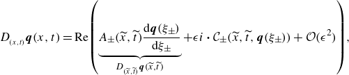 \begin{eqnarray} D_{_{(x,t)}}\boldsymbol{q}(x,t) = \mathrm{Re} {\left (\underbrace {A_\pm (\widetilde {x}, \widetilde {t}) \frac {{\rm d} \boldsymbol{q}(\xi _\pm )}{{\rm d}\xi _\pm }}_{D_{_{(\widetilde {x}, \widetilde {t})}}\boldsymbol{q}(\widetilde {x}, \widetilde {t})} + \epsilon i \,{\boldsymbol\cdot}\, \mathcal{C}_\pm (\widetilde {x}, \widetilde {t}, \boldsymbol{q}(\xi _\pm )) + \mathcal{O}(\epsilon ^2)\right )}, \end{eqnarray}
where the coefficient functions are
 \begin{eqnarray} A_+(\widetilde {x}, \widetilde {t}) = \frac {2 \lambda ^2 - \widetilde {x}(\lambda _{\widetilde {x}} + \lambda _{\widetilde {t}})}{\lambda ^2}, \qquad A_-(\widetilde {x}, \widetilde {t}) = -\frac {\widetilde {x}(\lambda _{\widetilde {x}} \lambda + \lambda _{\widetilde {t}})}{\lambda ^2}, \end{eqnarray}
where we denote
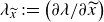 $ \lambda _{\widetilde {x}} := \big({\partial \lambda }/{\partial \widetilde {x}}\big)$
and
$ \lambda _{\widetilde {x}} := \big({\partial \lambda }/{\partial \widetilde {x}}\big)$
and
 $ \lambda _{\widetilde {t}} := \big({\partial \lambda }/{\partial \widetilde {t}}\big)$
. The terms
$ \lambda _{\widetilde {t}} := \big({\partial \lambda }/{\partial \widetilde {t}}\big)$
. The terms
 $ \mathcal{C}_\pm (\widetilde {x}, \widetilde {t}, \boldsymbol{q})$
denote first-order correction terms that arise from the chain rule and Taylor series expansions, and include all contributions involving second derivatives of
$ \mathcal{C}_\pm (\widetilde {x}, \widetilde {t}, \boldsymbol{q})$
denote first-order correction terms that arise from the chain rule and Taylor series expansions, and include all contributions involving second derivatives of
 $ \boldsymbol{q}$
, as well as spatial and temporal derivatives of
$ \boldsymbol{q}$
, as well as spatial and temporal derivatives of
 $ \lambda$
, evaluated at
$ \lambda$
, evaluated at
 $ (\widetilde {x}, \widetilde {t})$
. Therefore, to leading order, we can reconstruct (3.8) in the transformed
$ (\widetilde {x}, \widetilde {t})$
. Therefore, to leading order, we can reconstruct (3.8) in the transformed
 $(\widetilde {x},\widetilde {t})$
coordinate as
$(\widetilde {x},\widetilde {t})$
coordinate as
 \begin{eqnarray} \boldsymbol{v}^H \unicode{x1D63E} \left (D_{_{(x,t)}}\boldsymbol{q}(x,t)\right ) = \boldsymbol{v}^H \unicode{x1D63E} \ \mathrm{Re} {\left (D_{_{(\widetilde {x}, \widetilde {t})}}\boldsymbol{q}(\widetilde {x}, \widetilde {t})\right )}=\boldsymbol{0}. \end{eqnarray}
In the limit of weak spatiotemporal variation of
 $ \lambda$
, i.e.
$ \lambda$
, i.e.
 $ \lambda _{\widetilde {x}}, \lambda _{\widetilde {t}} \approx 0$
, we find that
$ \lambda _{\widetilde {x}}, \lambda _{\widetilde {t}} \approx 0$
, we find that
 $A_{\pm }$
become constant, yielding
$A_{\pm }$
become constant, yielding
 \begin{eqnarray} \boldsymbol{v}^H \unicode{x1D63E} \frac {{\rm d} \boldsymbol{q}(\xi ^R_{\pm })}{{\rm d}\xi ^R_{\pm }} = \boldsymbol{0}. \end{eqnarray}
Thus, a combination of flow variables in the transformed coordinate is conserved to leading order along the real component of the complex characteristics. Hence, to leading order, information propagates along the complex characteristic curve
 $\xi _{\pm }$
, with the direction governed approximately by the real part
$\xi _{\pm }$
, with the direction governed approximately by the real part
 $ \lambda ^R$
. Therefore, even in the complex setting, the effective characteristic curve in real space–time is given by
$ \lambda ^R$
. Therefore, even in the complex setting, the effective characteristic curve in real space–time is given by
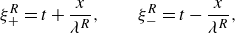 \begin{eqnarray} \xi _+^R = t + \frac {x}{\lambda ^R}, \qquad \xi _-^R = t - \frac {x}{\lambda ^R}, \end{eqnarray}
which reflects the fact that information propagation along complex characteristics on the leading order is tied to
 $\lambda ^R$
.
$\lambda ^R$
.


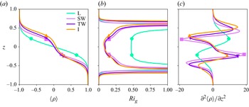


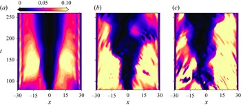


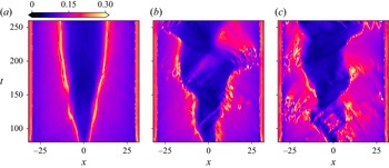


 Open access