Hypothesis from modeling

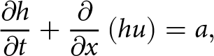
We use a 1D depth-integrated flowline model of a marine-terminating glacier with an unconfined ice shelf to understand how changes in basal friction near the grounding line are manifested in the ice-sheet surface geometry observable by satellites. In this study, we only consider the steady-state solutions of the discretized momentum (shallow shelf approximation; SSA) and mass conservation equations in the direction of ice flow ( $x$). Mass conservation in the glacier is governed by

(1)\begin{equation} \begin{aligned} \frac{\partial{h}} {\partial{t}} + \frac{\partial}{\partial{x}} \left(hu \right) = a , \end{aligned} \end{equation}

where $h$ is the ice thickness, $u$ is the ice velocity and $a$ is the surface mass balance of the glacier, which for the purposes of this study we assume is constant in space and time. We only consider the steady-state case where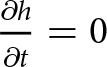 $\frac{\partial{h}} {\partial{t}}=0$. Conservation of momentum in the glacier is governed by

(2)\begin{equation} \begin{aligned} \frac{\partial} {\partial{x}} \bigg{[}2\bar{A}^{\nicefrac{-1}{n}} h\bigg{|}\frac{\partial{u}} {\partial{x}}\bigg{|}^{\nicefrac{1}{n}-1} \frac{\partial{u}} {\partial{x}}\bigg{]} -\theta C|u|^{m-1}u - \rho_igh\frac{\partial} {\partial{x}} (h-b) = 0 , \end{aligned} \end{equation}

where $\bar{A}$ is the depth-averaged rate factor in Glen’s flow law, $n$ is the Glen’s flow law exponent, $C$ is the sliding law coefficient, $m$ is the sliding law exponent, $\rho_i$ is the density of ice, $g$ is the acceleration due to gravity and $b$ is the depth of the ice-sheet below sea level. Unless otherwise noted, simulations in this study are conducted with a linearly down-sloping (prograde) bed everywhere ( $b(x) = b_0 - b_x x$). The first term on the left-hand side of Eqn (2) is the longitudinal stress, which plays an important role in the grounding zone under certain circumstances. The second term is basal friction, which is modified from Schoof (Reference Schoof2007) by introducing a nondimensional scaling factor $\theta$ (defined below). The third term is the driving stress.

The first boundary condition describes the floatation condition at the grounding line and is given by

(3)\begin{equation} \rho_i h(x=x_g) = \rho_w b(x=x_g), \end{equation}

where $x_g$ is the grounding line position. This equation acts as an additional constraint on the model and is included with the mass and momentum conservation equations to ensure that the grounding line is always located at a model grid point. All model parameter values are listed in Table 1, unless otherwise specified in the text.

Table 1.

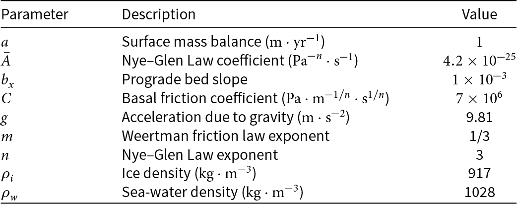
Parameter values for steady-state flowline simulations (unless otherwise specified).

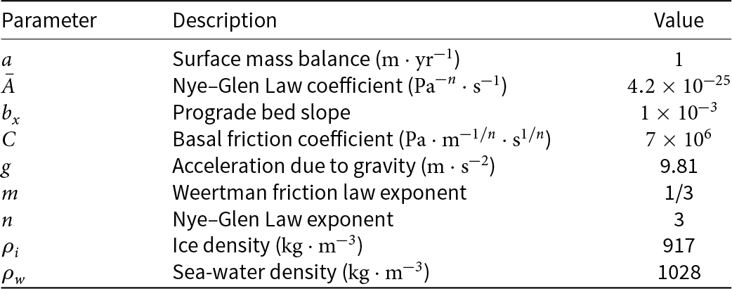
Table 1 Long description

The table lists parameter names, brief meanings, and numeric values used as inputs for steady-state flowline simulations. Surface mass balance is 1 meter per year, and the prograde bed slope is 0.001. Gravity is 9.81 meters per second squared. The Glen flow-law exponent is 3, with a corresponding flow-law coefficient of 4.2 times 10 to the minus 25 in pascal to the minus n per second. Basal friction uses a Weertman exponent of one third and a basal friction coefficient of 7 times 10 to the 6 in pascal times meter to the minus one over n times second to the one over n. Ice density is 917 kilograms per cubic meter, while seawater density is higher at 1028 kilograms per cubic meter. Values are presented as fixed constants for the simulations and do not indicate variability or uncertainty.

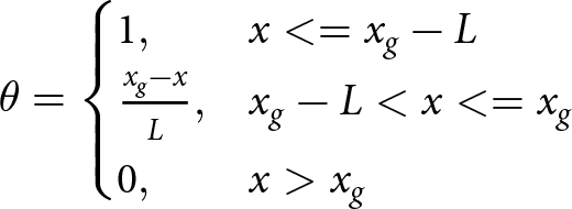
We model decreased basal friction in the grounding zone by prescribing idealized basal friction ‘ramps’ as illustrated in Fig. 1. We use a scaling variable $\theta$ to adjust the basal friction term of Eqn (2) such that it linearly decreases from one to zero over some distance $L$ upstream of the grounding line until it is exactly zero at the grounding line to be consistent with the boundary condition in Eqn (1). We define $\theta$ in Eqn (2) to vary with $x$ such that

(4)\begin{equation} \theta= \begin{cases} 1, & x \lt = x_g - L \\ \frac{x_g-x}{L},& x_g - L \lt x \lt = x_g\\ 0, & x \gt x_g \\ \end{cases} \end{equation}

This basal friction ramp produces an effective basal friction profile that is similar to the basal friction parameterizations described by Budd and others (Reference Budd, Keage and Blundy1979) and Tsai and others (Reference Tsai, Stewart and Thompson2015), but is easier to control. Physically, it can be thought of as resulting from either a transition to Coulomb sliding near the grounding line or the result of basal lubrication by sea water. It differs from the Tsai friction law in that basal friction is still velocity-dependent even in the ramp region, and from both Budd and Tsai laws in that it has no explicit dependence on effective pressure.

We use an iterative numerical root-finding method to solve Eqns (1)–(3) simultaneously with a basal friction ramp of some specified length. These cases are compared to a control case without a basal friction ramp ( $L$ = 0 km). We use a numerical approach adapted from Schoof (Reference Schoof2007), where the model grid is stretched to maintain fine horizontal grid resolution ( $\Delta x \sim$ 100–200 m, though exact grid resolution stretches with the grounding line position) just upstream of the grounding line. This numerical approach ensures that the extent of each $L$ is well resolved and contained entirely within the refined grid. The flowline model is available as a public repository (Robel, Reference Robel2021) and has been used and benchmarked in several previous studies (e.g., Robel and others, Reference Robel, Roe and Haseloff2018; Christian and others, Reference Christian, Robel and Catania2022; Kodama and others, Reference Kodama2025).

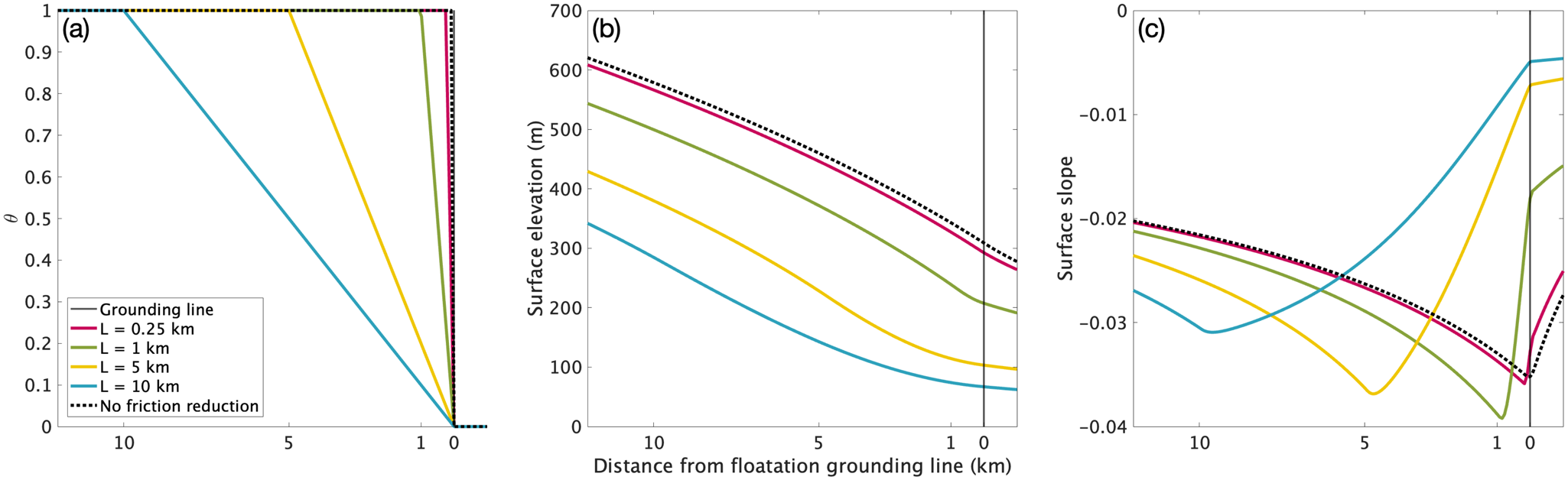
In Fig. 1b, we plot the surface slope profiles for each tested friction ramp length. We find that there is a distinct surface slope profile for friction ramps of 1 km and longer as compared to a control case with no friction ramp. In the control profile, the surface slope break from a steep to a shallow slope occurs at the grounding line, which by the mathematical definition of this model (Eqn (2)) is the point at which ice is thin enough to float in sea water and the last contact between ice and the bed. In cases with a friction ramp, the characteristic slope break where surface slope begins to become less steep instead occurs just downstream from the point where basal friction begins to decrease. This slope break is associated with a change in the concavity of the ice surface (i.e., the second derivative of surface slope is zero) and is distinct from the transition to near constant slope that still occurs at the grounding line. The steepest surface slope is 200–300 m downstream of the friction ramp offset in our simulations. We find that even in simulations with double and quadruple grid resolution in the grounded region (not plotted), the offset distance does not change with resolution. Thus, we conclude that this offset is capturing the longitudinal length scale associated with surface expression of basal friction.

Figure 1.

(a) Basal friction ramps of varying lengths $L$ upstream of the floatation grounding line and the control friction scenario. (b) Surface elevation profiles over basal friction ramps of varying lengths $L$ upstream of the floatation grounding line compared to the control friction scenario. (c) Same as (b), but for surface slope profiles.

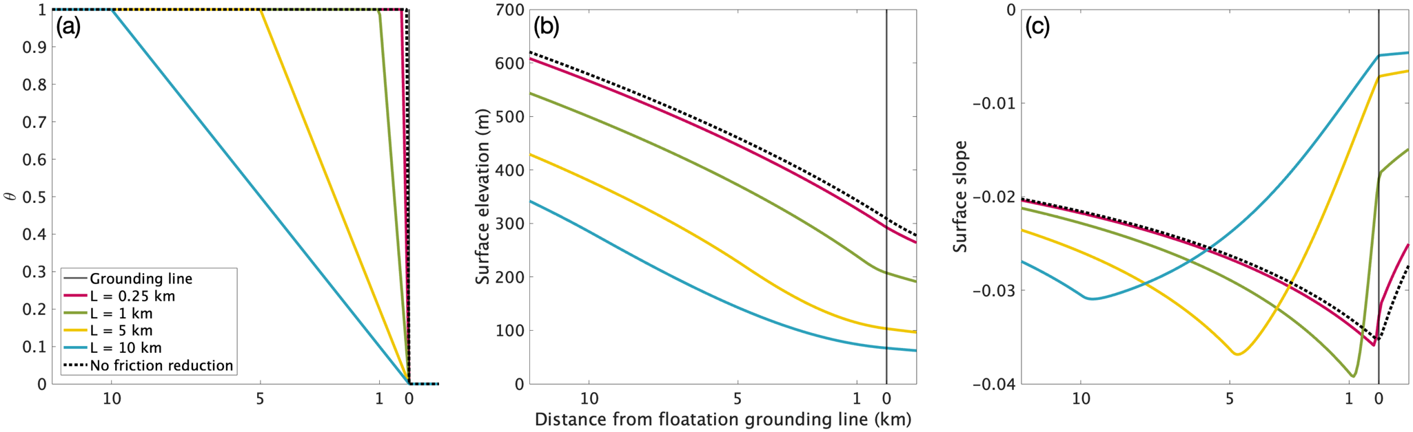
Figure 1 Long description

The image A showing a line graph labeled (a). The horizontal axis label is “Distance from floatation grounding line (km)”. The horizontal axis shows 10, 5, 0. The vertical axis label is “Basal friction”. The vertical axis shows 0.0 to 1.0. A legend lists: “Control”, “L = 1 km”, “L = 5 km”, “L = 10 km”, “L = 50 km”. The plotted lines decrease toward 0 km. The “Control” line stays near 1.0 across most of the distance range and drops close to 0 near 0 km. The “L = 1 km” line stays near 1.0 until close to 0 km, then drops close to 0. The “L = 5 km” line decreases from near 1.0 at 10 km to 0 at 0 km. The “L = 10 km” line decreases from near 1.0 at 10 km to 0 at 0 km, with a steeper drop closer to 0 km than the “L = 5 km” line. The “L = 50 km” line stays near 1.0 and drops close to 0 very near 0 km. The image B showing a line graph labeled (b). The horizontal axis label is “Distance from floatation grounding line (km)”. The horizontal axis shows 10, 5, 0. The vertical axis label is “Surface elevation (m)”. The vertical axis shows 0 to 700. Multiple lines are plotted, corresponding to the same set of scenarios as in (a). All lines slope downward from 10 km toward 0 km. At about 10 km, the highest line is near 600 m and the lowest line is near 300 m. Near 0 km, the lines converge around roughly 100 m to 200 m. The separation between lines is larger around 10 km and smaller near 0 km. The image C showing a line graph labeled (c). The horizontal axis label is “Distance from floatation grounding line (km)”. The horizontal axis shows 10, 5, 0. The vertical axis label is “Surface slope”. The vertical axis shows negative 0.04 to negative 0.01. Multiple lines are plotted, corresponding to the same set of scenarios as in (a). Several lines start near about negative 0.02 to negative 0.03 around 10 km and become more negative toward a minimum near about negative 0.04 before rising toward less negative values near 0 km. One line rises toward about negative 0.01 near 0 km. A crossing between two lines occurs around the mid-range of the horizontal axis. All three graphs use the same horizontal axis label, “Distance from floatation grounding line (km)”, to compare how basal friction, surface elevation and surface slope vary across the same distance range for the listed scenarios.

We thus conclude from these simulations that a regime of decreasing basal friction upstream of the grounding line is accompanied by a surface slope break that is not co-located with the grounding line as defined by the floatation thickness or point of last contact with the bed. The slope breaks associated with the onset of the basal friction ramp are both larger and oriented in a different direction (steep to shallow) from the second slope breaks associated with each simulation’s contact grounding line. From these results, we hypothesize that the onset of reduced basal friction upstream of the floatation/contact grounding line will be accompanied by a surface slope break, which could be observable by satellite measurements of surface elevation.

Modeling additional potential causes of surface slope breaks

Our hypothesis from modeling connects a decreased basal friction regime to surface slope breaks displaced upstream from the floatation grounding line, but other bed properties may also have surface expression near the grounding line. We simulate the surface expressions of basal melt and changes in bed slope for comparison to our decreased basal friction scenario.

Impact of basal melt

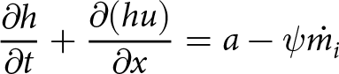
To investigate the surface expression changes with basal melt upstream of the grounding line (i.e., similar to the melt from sea-water intrusion modeled in Robel and others, Reference Robel, Wilson and Seroussi2022b), we experimented with the introduction of a basal melt parameter to the mass continuity equation for grounded ice (Eqn (1)) such that

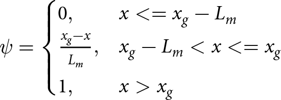
(5)\begin{equation} \frac{\partial{h}} {\partial{t}} + \frac{\partial{(hu)}} {\partial{x}} = a - \psi \dot{m_i} \end{equation}

where $\dot{m_i}$ is the rate of basal melt (melt being positive $\dot{m_i}$), and $\psi$ is a nondimensional scaling factor. We apply an initial basal melt rate $\dot{m_i}$ at the grounding line, then linearly decrease the basal melt rate from the floatation grounding line to zero across some distance $L_m$ upstream of the grounding line, much like the friction ramp defined in Eqn (4). We define $\psi$ in Eqn (5) to vary with $x$ such that

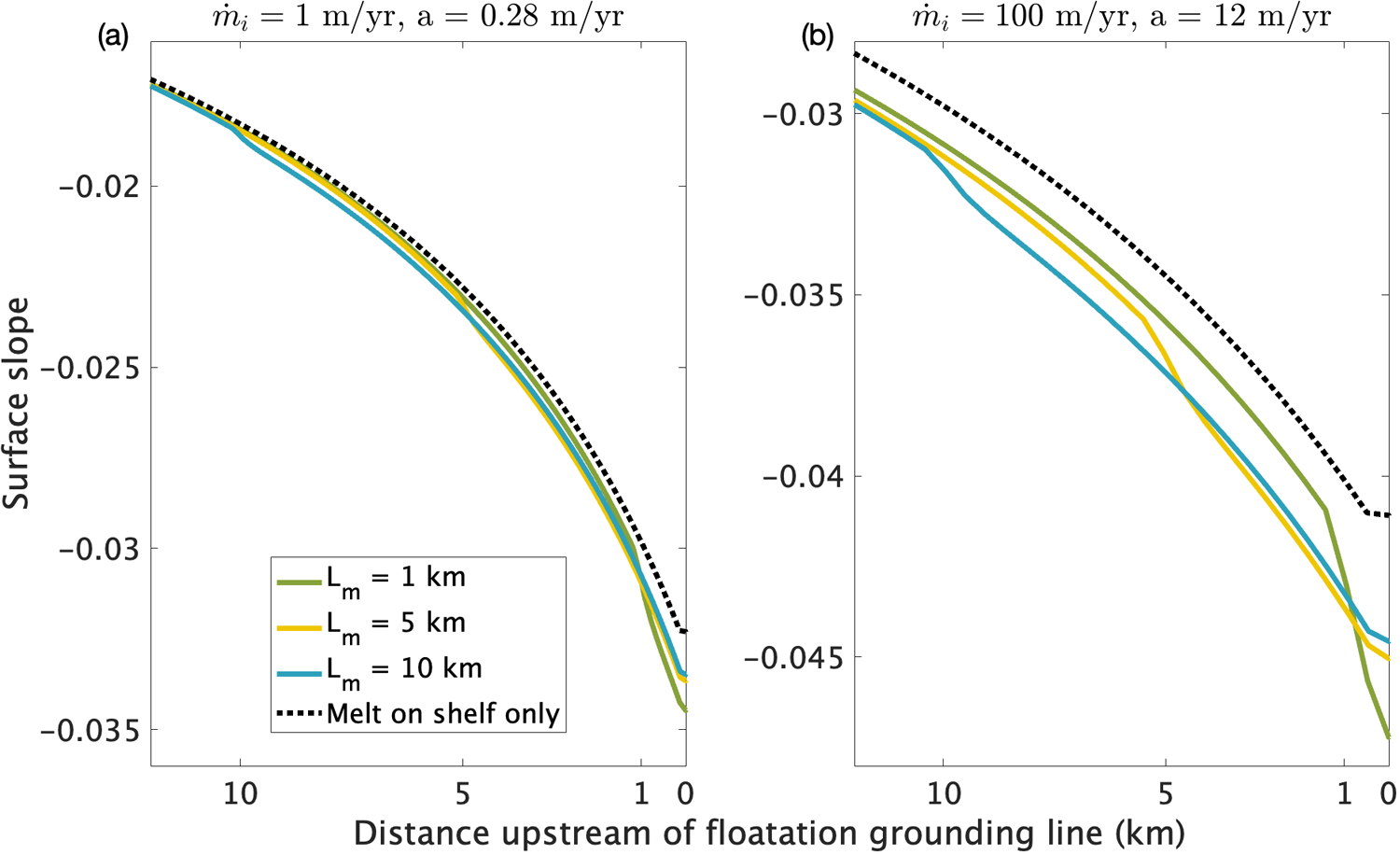
(6)\begin{equation} \psi = \begin{cases} 0, & x \lt = x_g - L_m \\ \frac{x_g-x}{L_m},& x_g - L_m \lt x \lt = x_g\\ 1, & x \gt x_g \\ \end{cases} \end{equation}

We simultaneously solve Eqns (2) and (5) and with $\theta=1$, thereby removing the basal friction ramp and isolating the effect of basal melt. We tested the impact of the magnitude of basal melt by considering two cases: a case with a low basal melt rate and SMB (Fig. 2a), and a case with high basal melt rate and high SMB (Fig. 2b). In the high basal melt rate case, increased SMB is necessary to be able to achieve a steady state. In both cases, we consider a baseline with only basal melting on the ice shelf (black dashed lines) and then basal melt ramps where basal melt decreases to zero upstream of the grounding line over distances ( $L_m$) of 1, 5 and 10 km (green, yellow and blue lines, respectively), as in Robel and others (Reference Robel, Wilson and Seroussi2022b). In all cases, there is a surface slope steepening at the onset of basal melting, as shown in Fig. 2. The magnitude of the surface steepening is controlled by the magnitude of basal melting.

Figure 2.

Surface slope profiles over basal melt ramps of varying lengths $L_m$ upstream of the floatation grounding line. (a) Low melt rate and SMB (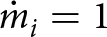 $\dot{m}_i = 1$ m/yr, $a = 0.28$ m/yr). (b) High melt rate and SMB (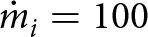 $\dot{m}_i = 100$ m/yr,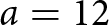 $a = 12$ m/yr).

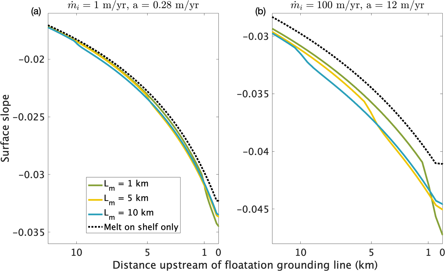
Figure 2 Long description

Panel (a) shows surface slope profiles with a low melt rate (m dot subscript i equals 1 meter per year, a equals 0.28 meter per year). The x-axis represents distance upstream of the floatation grounding line in kilometers, ranging from 10 to 0. The y-axis represents surface slope, ranging from negative 0.035 to negative 0.02. Four lines are shown: L subscript m equals 1 kilometer, L subscript m equals 5 kilometer, L subscript m equals 10 kilometer and melt on shelf only (dashed line). The dashed line is consistently above the solid lines, indicating less negative slope closer to the grounding line. At 10 kilometers, the slope is approximately negative 0.035 for all lines, while at 1 kilometer, the dashed line shows a slope of about negative 0.02, diverging from the solid lines. Panel (b) displays surface slope profiles with a high melt rate (m dot subscript i equals 100 meter per year, a equals 12 meter per year). The axes are similar to panel (a). The dashed line remains above the solid lines, showing less negative slope. At 10 kilometers, the slope is approximately negative 0.045 for all lines and at 1 kilometer, the dashed line shows a slope of about negative 0.03. The graph demonstrates the sensitivity of surface slope to melt-length scale L subscript m and melt-rate scenario between panels. The dashed line indicates the effect of melt on shelf only, showing how basal melt impacts surface slope steepening.

Basal melting upstream of the grounding line produces a subtle surface slope break, but one that is in the direction of steepening downstream. This slope break has the opposite sign of the surface slope break generated by the onset of reduced basal friction, which is still by far the largest slope break, even in these cases with a basal melt ramp upstream of the grounding line. In steady state, the ice surface profile is set by a balance between the ice flux divergence and surface/basal mass balances, which remain relatively constant over most of the glacier. In the grounding zone (within a few kilometers upstream of the grounding line), the flux divergence is large compared to the addition of the basal melt ramp. Consequently, the mass balance is largely unchanged by such a basal melt ramp and leads to a relatively weak surface slope expression. Basal melt under grounded ice can still lubricate the bed and contribute to a decreased basal friction regime as described in our hypothesis, so the role of basal melt in the development of low-friction basal regimes should not be ignored.

Impact of a ridge in bed topography

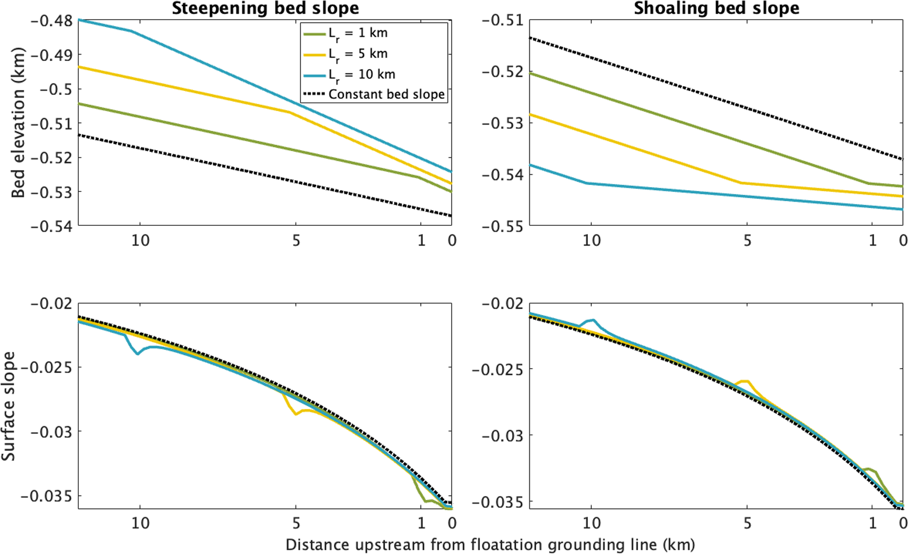
We also model the surface expression of changes to the bed slope near the grounding line to compare with the surface expression of a friction ramp and determine whether one could be confused for another. Till deposition has been observed to occur at the grounding line of ice streams (Anandakrishnan and others, Reference Anandakrishnan, Catania, Alley and Horgan2007), though it is not yet settled whether deposition occurs upstream or downstream of the flexural grounding line (Christian and others, Reference Christian, Robel, Catania, Stearns, Miller and Garcia2026). We test two bed topography regimes: first, a regime where the bed slope steepens by a factor of 2, and second, where the bed slope shoals by a factor of 4. For each bed topography considered, we model the change in surface slope occurring at lengths $L_r$ = 1, 5 and 10 km upstream of the grounding line. In each simulation with a ridge, we slightly raise or lower the entire topography to produce a grounding line position at approximately the same location as in the constant bed slope case. Figure 3 visualizes the results.

Figure 3.

Bed elevation (a, c) and surface slope (b, d) for regime of steepening (a, b) and shoaling (c, d) bed slopes at varying lengths $L_r$ upstream of the floatation grounding line.

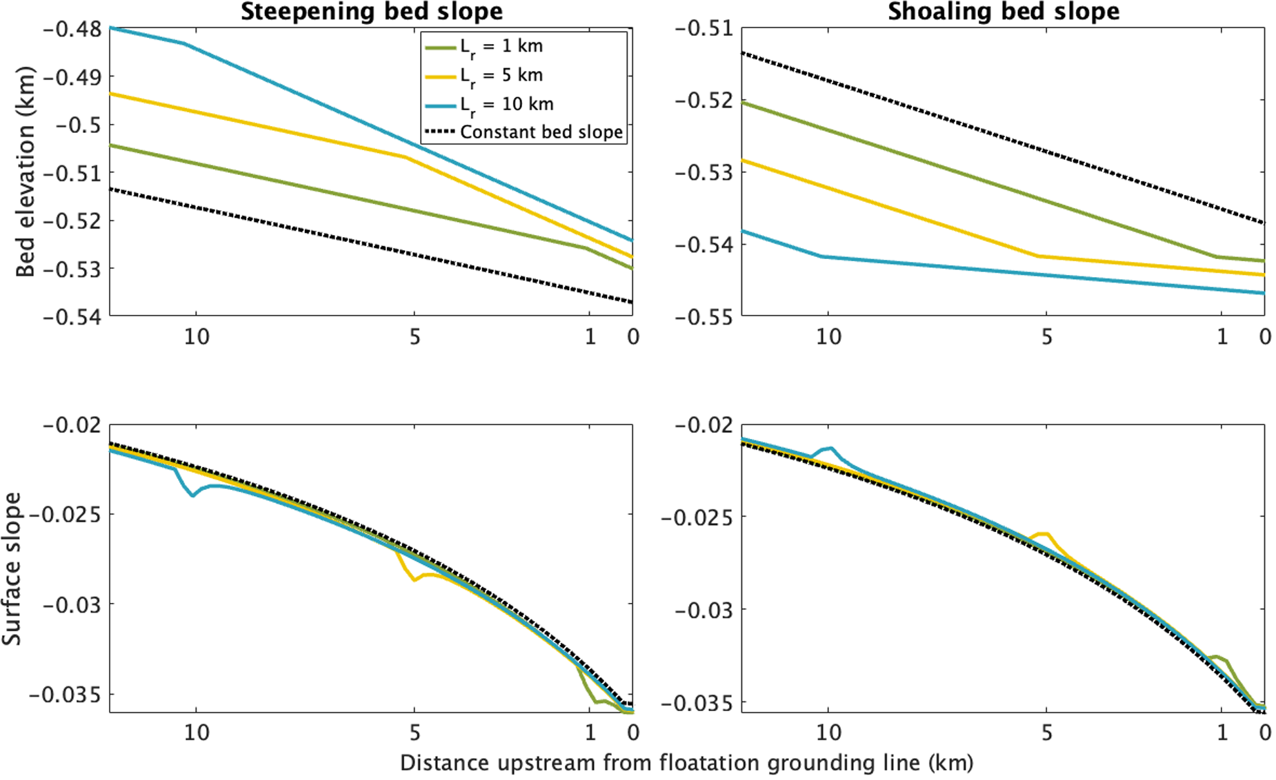
Figure 3 Long description

The image A showing a line graph titled “Steepening bed slope”. The x-axis label is “Distance upstream from floatation grounding line (km)”. The x-axis shows 10, 5, 1, 0. The y-axis label is “Bed elevation (km)”. The y-axis shows negative 0.48, negative 0.49, negative 0.5, negative 0.51, negative 0.52, negative 0.53, negative 0.54. A legend lists “L subscript r equals 1 km”, “L subscript r equals 5 km”, “L subscript r equals 10 km” and “Constant bed slope”. Four lines descend from x equals 10 toward x equals 0. The “Constant bed slope” line is a dashed line that stays below the other lines across the plotted distance. The “L subscript r equals 1 km” line starts near negative 0.48 at x equals 10 and ends near negative 0.52 at x equals 0. The “L subscript r equals 5 km” line starts near negative 0.49 at x equals 10 and ends near negative 0.525 at x equals 0. The “L subscript r equals 10 km” line starts near negative 0.505 at x equals 10 and ends near negative 0.53 at x equals 0. The lines are closer together near x equals 0 than near x equals 10. The image B showing a line graph titled “Shoaling bed slope”. The x-axis label is “Distance upstream from floatation grounding line (km)”. The x-axis shows 10, 5, 1, 0. The y-axis label is “Bed elevation (km)”. The y-axis shows negative 0.51, negative 0.52, negative 0.53, negative 0.54, negative 0.55. Four lines descend from x equals 10 toward x equals 0. One dashed line runs above the other lines across the plotted distance. The other three lines are separated near x equals 10 and become closer near x equals 0, with endpoints clustered near negative 0.545 to negative 0.55 at x equals 0. The image C showing a line graph. The x-axis label is “Distance upstream from floatation grounding line (km)”. The x-axis shows 10, 5, 1, 0. The y-axis label is “Surface slope”. The y-axis shows negative 0.02, negative 0.025, negative 0.03, negative 0.035. Multiple lines follow a similar downward curve from near negative 0.02 at x equals 10 toward near negative 0.035 at x equals 0. Small deviations between lines appear around x values near 10 and near 5 and the lines converge near x equals 0. The image D showing a line graph. The x-axis label is “Distance upstream from floatation grounding line (km)”. The x-axis shows 10, 5, 1, 0. The y-axis label is “Surface slope”. The y-axis shows negative 0.02, negative 0.025, negative 0.03, negative 0.035. Multiple lines follow a similar downward curve from near negative 0.02 at x equals 10 toward near negative 0.035 at x equals 0. A small local rise is visible near x values close to 10 on one line and the lines converge near x equals 0.

When the onset of the steeper or shallowing bed slope occurs 5 or 10 km upstream of the grounding line, the surface slope briefly changes (over $ \lt 1$ km distance) at the location of the bed slope break and then quickly recovers to the background surface slope. When the onset of the steeper bed slope occurs at just 1 km upstream of the grounding line, the depression in the surface slope is sufficiently localized that it would be difficult to discern from the surface slope break at the grounding line. The local extreme in surface slope occurs upstream of the floatation grounding line, so a steepening bed slope near the grounding line can manifest in a surface slope break displaced upstream from the floatation grounding line. However, the change in surface slope is considerably less than modeled for a change in basal friction.

We conclude that the surface expression of a break in bed slope near the grounding line will not be mistaken for the low basal friction regime described by the hypothesis described previously due to its small magnitude and localization. Initial simulations with isolated bed bumps similar to those plotted in Robel and others (Reference Robel, Pegler, Catania, Felikson and Simkins2022a, and not plotted here) produce small isolated surface expressions with little resemblance to the surface expression of the friction ramp.

Analysis of ICESat-2 data

The simulations above suggest a potential method for detecting regions of decreased basal friction just upstream of grounding lines using ice surface features observable from satellites. Many prior studies have used observations to constrain the grounding line position with different methods. Prior to the recent era of accurate, repeat-track altimetry with substantial coverage over Antarctica, surface slope break (denoted Point $I_b$ hereafter) and floatation thickness were the most commonly used indicators of grounding line position (Herzfeld and others, Reference Herzfeld, Lingle and Lee1994; Brunt and others, Reference Brunt, Fricker, Padman, Scambos and O’Neel2010). More recently, the advent of repeat-track altimetry and InSAR satellites has enabled the identification of regions of ice shelf flexure in response to tides. The inland limit of tidal flexure (denoted Point F hereafter) is a reliable indicator of the location where ice is last in contact with the bed, even if friction is low here (since tides induce detectable vertical motion of the ice surface where the ice base does not rest on the bed). Early methods for locating the grounding line (Horgan and Anandakrishnan, Reference Horgan and Anandakrishnan2006; Scambos and others, Reference Scambos, Haran, Fahnestock, Painter and Bohlander2007) assumed that a surface slope break (Point $I_b$) is co-located with the last point of ice contact with the bed (Point F). Here we instead hypothesize that the surface slope break, as detected by altimetry, is the location of the onset of reduced basal friction at the bed, which may not always coincide with the last point of ice contact with the bed. We measure the extent of this ‘displacement’ of a detectable surface slope break from the inland limit of tidal flexure using an existing dataset of these points derived from satellite altimetry.

Algorithm to calculate the along-flow displacement of surface slope break

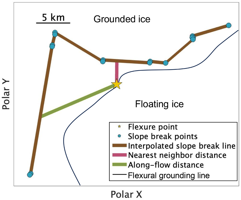
The objective of our analysis is to evaluate whether $I_b$ points, as identified by Li and others (Reference Li, Dawson, Chuter and Bamber2022), reside upstream or downstream of Point F, and then to evaluate the distance between these points. The general idea of the algorithm is that for each Point F, we construct a local curve of the $I_b$ points within 10 km of Point F (referred to here as Curve $I_b$). Then, we calculate the distance between Point F and its Curve $I_b$ along both the nearest neighbor direction and the local flow direction. Figure 4 illustrates one example of how this algorithm works.

Figure 4.

Exemplar illustration of the inputs and outputs of the along-flow distance algorithm, including the flexure point (Point F) and slope break points (Point $I_b$) from Li and others (Reference Li, Dawson, Chuter and Bamber2022), the interpolated line of slope break points (Curve $I_b$), the nearest neighbor distance line and the along-flow distance line.

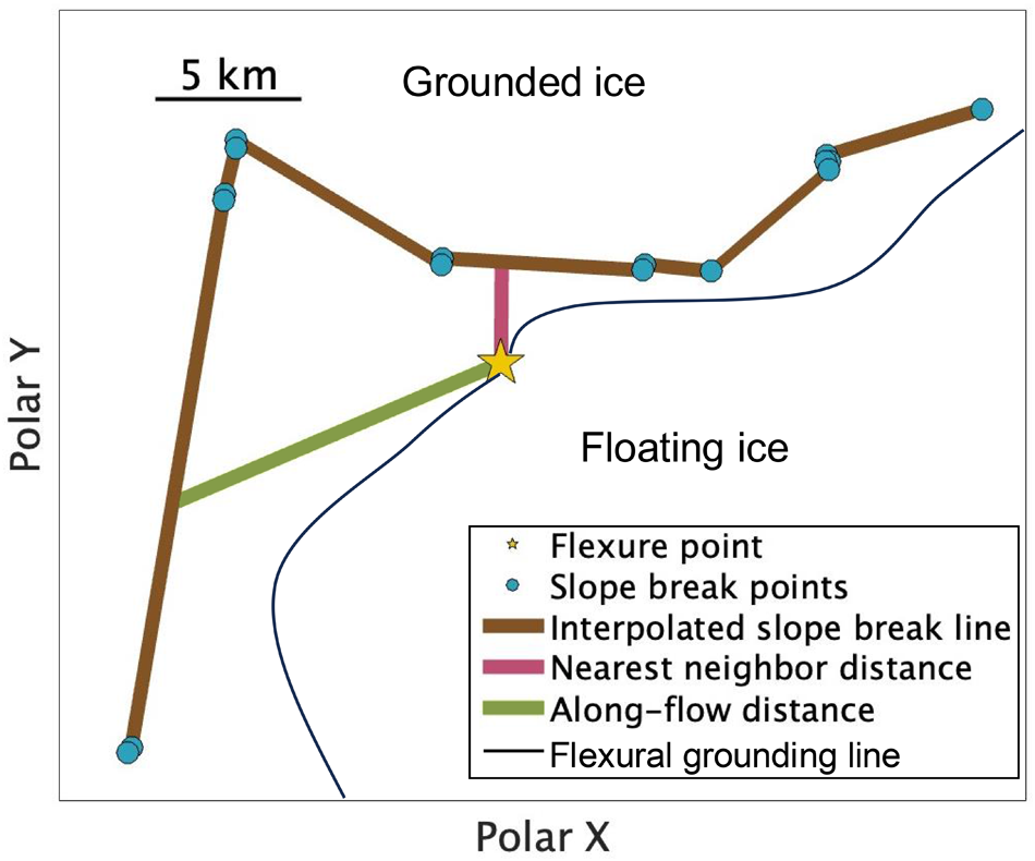
Figure 4 Long description

The diagram illustrates the along-flow distance algorithm in polar coordinates, showing the relationship between grounded and floating ice. The x-axis is labeled 'Polar X' and the y-axis is labeled 'Polar Y'. A polyline path with markers represents slope break points, connecting grounded ice to floating ice. A flexure point is marked on this polyline near the boundary curve separating grounded ice from floating ice. Lines radiate from the flexure point, labeled 'Nearest neighbor distance' and 'Along-flow distance', measuring connections to slope break points and the grounding line. The legend includes 'Flexure point', 'Slope break points', 'Interpolated slope break line', 'Nearest neighbor distance line', 'Along-flow distance line' and 'Flexural grounding line'. The scale indicator '5 km' applies to the map scale. The diagram demonstrates how the flexure point serves as the origin for measuring distances and connections within the ice flow context.

First, we eliminate all Point $I_b$ and Point F data lying within ice rises, as identified in the Antarctic Mapping Tool mask (Rignot and others, Reference Rignot, Jacobs, Mouginot and Scheuchl2013; Greene and others, Reference Greene, Gwyther and Blankenship2017; Mouginot and Rignot, Reference Mouginot and Rignot2017), to ensure small ice rises with unreliable grounding line estimates do not bias our analysis. Second, for each Point F, we find the set of $I_b$ points within 10 km of Point F. To create Curve $I_b$, we linearly interpolate the points with a spacing of 10 m according to the ICESat-2 ordering as in the data provided in Li and others (Reference Li, Dawson, Chuter and Bamber2022), which is approximately radial with respect to the South Pole. In this dataset, $I_b$ points are ordered by ICESat-2 track. While in some locations of strongly sinuous grounding line, this may lead to local interpolation error, such locations are likely to be filtered out by our quality control algorithm described further below. Third, we calculate the nearest neighbor distance between Point F and its Curve $I_b$ for comparison to its along-flow distance. Because the data are projected onto an Antarctic polar stereographic grid, we calculate the local Euclidean distance between Point F and all points of the Curve $I_b$. Fourth, we calculate the along-flow distance between Point F and its Curve $I_b$. To determine the local flow direction from each Point F, we use the gradient of ice surface elevation determined from the MEaSUREs BedMachine product, Version 3 (Morlighem, Reference Morlighem2022).

We assume that the surface gradient points in the flow direction (downstream). The algorithm sequentially checks whether the down-gradient direction at Point F intersects with the Curve $I_b$, and if not, then it checks whether the up-gradient direction at Point F intersects with the Curve $I_b$. Based on these checks, Curve $I_b$ is classified as either being downstream or upstream of Point F. If neither flow direction is found to intersect with the interpolated Curve $I_b$ within 50 km, then no along-flow distance is reported. Finally, for those F points that have an along-flow Curve $I_b$, we quality control our analysis by calculating the surface gradient vector of Point $I_b$ to determine if flowlines are strongly variable in this region. If the angle between the surface gradient vectors at Point F and the along-flow Point $I_b$ is greater than 90 degrees, we flag this Point F–Point $I_b$ pair as being abnormal.

Results

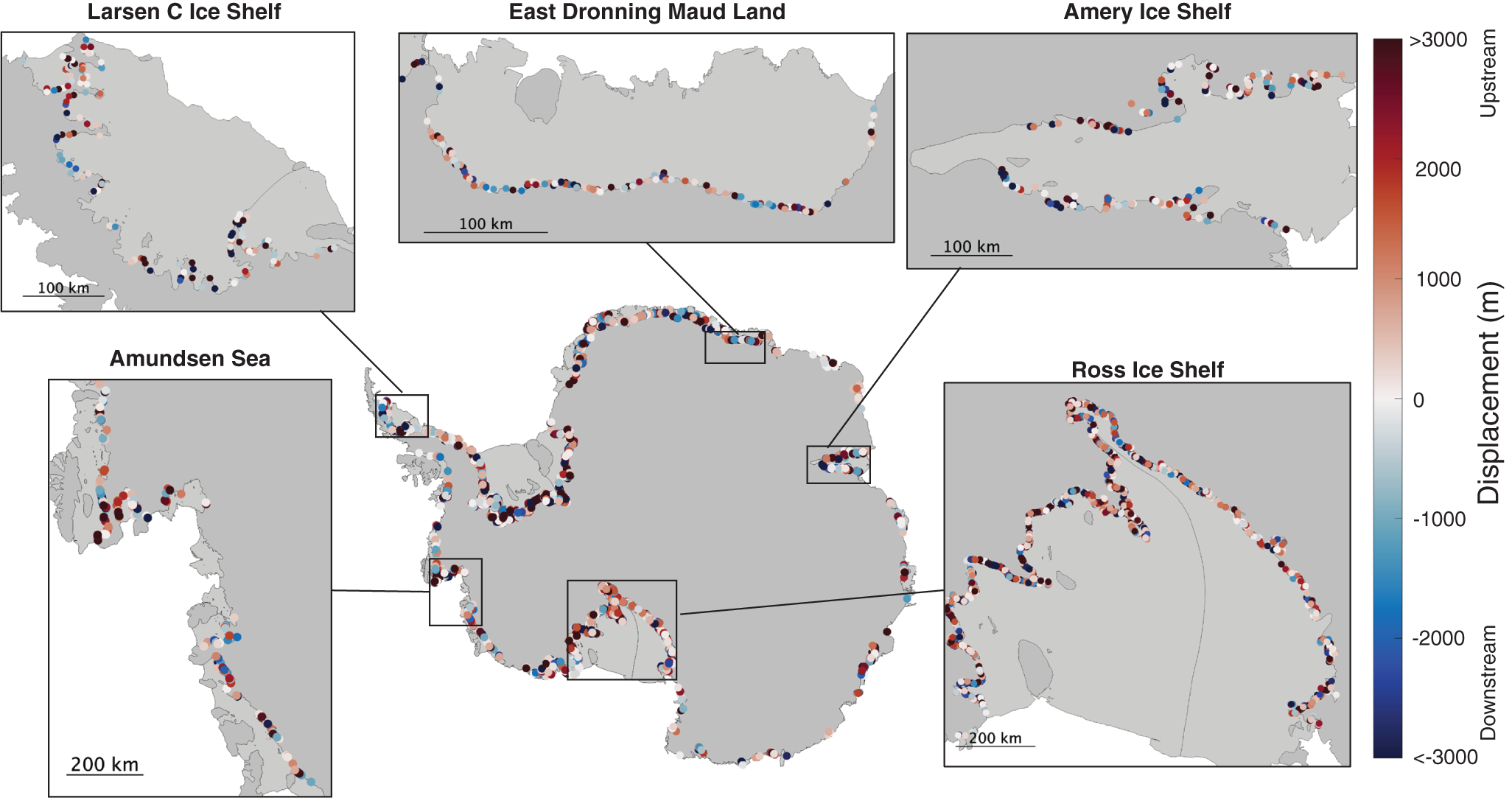
Of the 21 346 F points in the Li and others (Reference Li, Dawson, Chuter and Bamber2022) dataset, the algorithm found 12 807 (50.9%) with upstream displaced $I_b$ points and 6049 (28.3%) with downstream displaced $I_b$ points. The algorithm was unable to identify an along-flow Point $I_b$ for 2430 (11.4%) F points. The remaining F points are associated with ice rises. For the upstream displaced points, the median distance across the Antarctic ice sheet is 1260 m, and the mean distance is 2019 m. For the downstream displaced points, the median distance is 1752 m, and the mean distance is 2394 m. When we filter the results to only include points where the difference in the surface gradient between Point F and Point $I_b$ is less than 90 degrees (i.e., the slope break occurs along a flowline line reaching the InSAR-derived grounding line), the median and the mean distance for the upstream points is 1085 and 1855 m, respectively (from 10 084 data points, or 84.8% of the total upstream displaced points). For filtered downstream points, the mean and the median distance are 2220 and 1540 m, respectively (from 4634 data points, or 76.6% of the total downstream points). Figure 5 is a map plotting all $I_b$ not flagged as ‘abnormal’ with points upstream from F points colored in red, and points downstream from F points colored in blue (and denoted as a negative value).

Figure 5 includes more detailed maps of locations where ICESat-2 data indicate surface slope breaks displaced from flexural grounding lines. In particular, we note particularly far upstream displacements (i.e., multiple kilometers) along the active ice streams along the Siple Coast of the Ross Ice Shelf and the Queen Elizabeth Land portion of the Filchner–Ronne Ice Shelf. Though there are some portions of the Amundsen Sea and Larsen C grounding lines with substantial upstream displacements, ICESat-2 tracks along the main trunks of Thwaites and Pine Island glaciers were eliminated by the quality control algorithm, due to the strongly sinuous nature of the grounding line in this region. Downstream displacements are scattered around the Antarctic grounding line, but there are some notable clusters at the stagnant Kamb Ice Stream and the glaciers flowing into Cabinet Inlet in Larsen C Ice Shelf.

Figure 5.

F points from Li and others (Reference Li, Dawson, Chuter and Bamber2022) with upstream or downstream interpolated Point $I_b$ as identified by the along-flow distance algorithm, where the surface gradient differences between Point F and interpolated Point $I_b$ are less than 90 degrees. F points are colored by their distance from their corresponding interpolated Point $I_b$. Five insets highlight the findings for different regions.

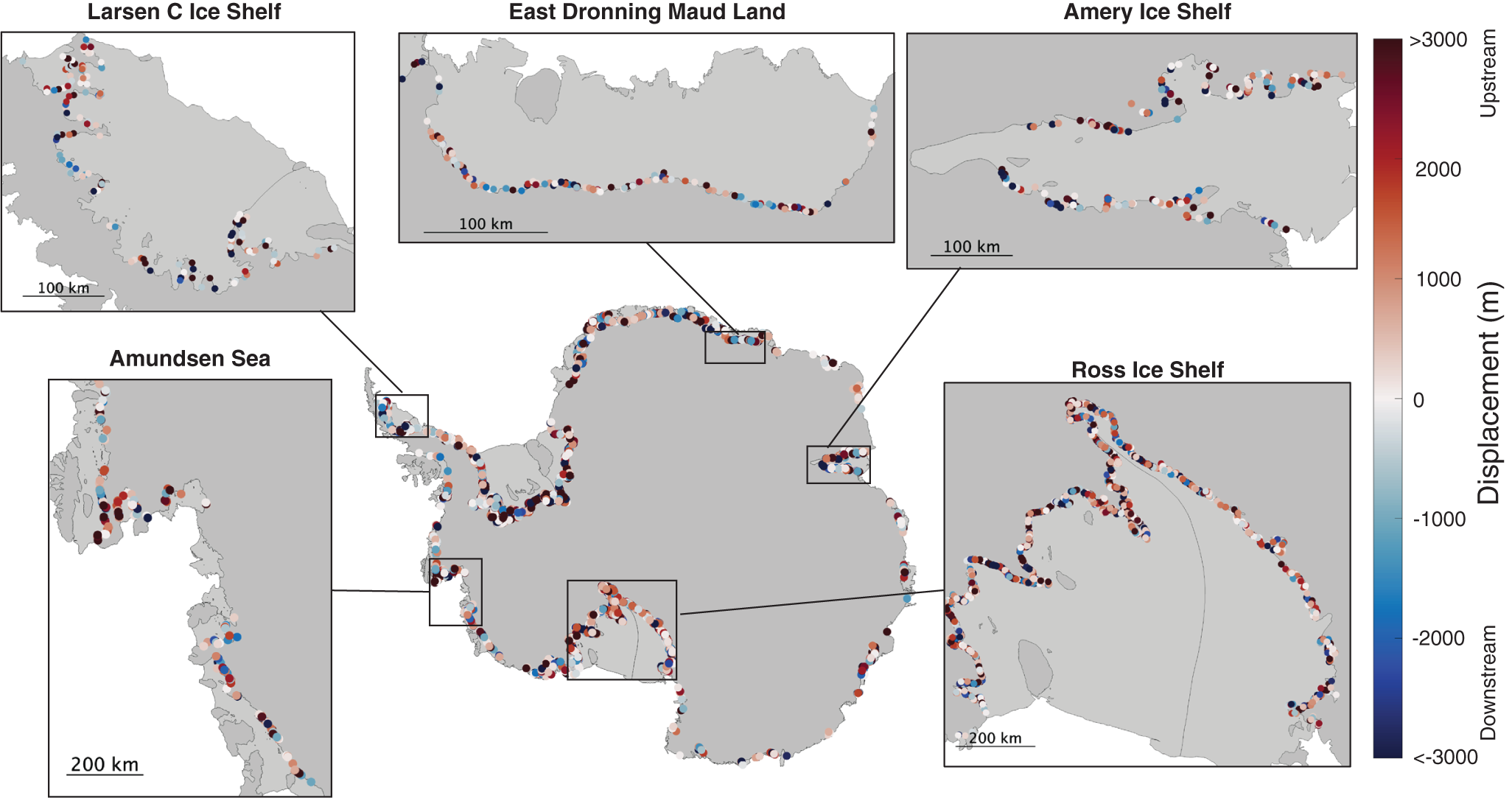
Figure 5 Long description

The map of Antarctica displays the displacement of F points across various ice shelves and seas, with five insets focusing on specific regions. The displacement is measured in meters, ranging from upstream (>3000 m) to downstream (<-3000 m), as indicated by the color gradient on the right. A) Larsen C Ice Shelf: Points are distributed along the shelf, with a mix of upstream and downstream displacements. B) East Dronning Maud Land: Points are scattered along the coast, showing varied displacement patterns. C) Amery Ice Shelf: Points are spread across the shelf, indicating both upstream and downstream movements. D) Amundsen Sea: Points are concentrated along the coast, with significant upstream displacement visible. E) Ross Ice Shelf: Points are densely packed along the shelf, showing a range of displacements. The map provides a comprehensive view of displacement patterns across these regions, highlighting areas of significant movement.

This analysis connects our hypothesis from modeling with real-world observations of displacement between surface slope breaks and ‘true’ flexural grounding lines. The prevalence of regions with such upstream displacement around Antarctica could, with further investigation, potentially be explained by low-friction basal regimes. The implications and caveats of this work are discussed in the following section.

Data availability statement

All code used to run models, analyze data and generate figures in this study is publicly available at the following GitHub repository: https://github.com/aarobel/Surface-Expression-Of-Low-Basal-Friction. This repository also includes a pre-processed dataset (ICESat2_Li2022_frictionramplength.csv) listing the locations of grounding line points with upstream displaced surface slope breaks.