


1. Introduction
At present, ion and Hall-effect thrusters are mature technologies employed in many space missions (Goebel & Katz Reference Goebel and Katz2008). At the same time, recent advances in plasma-based propulsion systems have led to the development of electromagnetic radio-frequency (RF) plasma generation and acceleration systems, termed magnetically enhanced plasma thrusters (MEPTs) (Manente et al. Reference Manente, Trezzolani, Magarotto, Fantino, Selmo, Bellomo, Toson and Pavarin2019). The absence of neutralizers, and electrodes in contact with the plasma makes the MEPT a simple and potentially long-life technology.
Magnetically enhanced plasma thrusters have been studied and developed in many international projects by both research centres and industry. Several studies concern helicon plasma thrusters (HPTs), namely systems that can be included in the broader category of MEPTs. The first works on HPTs date back to the early 2000s and led to the development of a thruster operating in the 0.25–0.7 kW range at the Australian National University (Boswell & Charles Reference Boswell and Charles2003; Pottinger et al. Reference Pottinger, Lappas, Charles and Boswell2011; Takahashi et al. Reference Takahashi, Charles, Boswell and Ando2014). At the University of Padua, a 50 W HPT was designed, developed and tested during the HPH.COM project (Pavarin et al. Reference Pavarin, Ferri, Manente, and Rondini, and Curreli, Guclu, Melazzi, Suman, Bianchini and Packan2010). The Massachusetts Institute of Technology and Madrid University have developed HPTs operating in the 0.5–1 kW range (Batishchev Reference Batishchev2009; Merino et al. Reference Merino, Navarro, Casado, Ahedo, Gómez, Ruiz, Bosch and del Amo2015). Seminal research on the dynamics of HPTs has been conducted at Tohoku University (Takahashi Reference Takahashi2019). Particularly remarkable is the development of a HPT working in the 5 kW power range that provides the highest thruster efficiency ever measured with these devices, namely 20 % (Takahashi Reference Takahashi2021). Also, HPTs specifically designed for CubeSats and operating in the 10–50 W range have been developed at the University of Michigan (Sheehan et al. Reference Sheehan, Collard, Ebersohn and Longmier2015). Helicon plasma thrusters are also promising candidates for application to atmosphere-breathing electric propulsion, under investigation at the University of Stuttgart (Romano et al. Reference Romano, Chan, Herdrich, Traub, Fasoulas, Roberts, Smith, Edmondson, Haigh and Crisp2020). Finally, other research centres that have studied thoroughly the dynamics of HPTs are Tokyo University (Shinohara et al. Reference Shinohara, Nishida, Tanikawa, Hada, Funaki and Shamrai2014) and Washington University (Ziemba et al. Reference Ziemba, Carscadden, Slough, Prager and Winglee2005).
A MEPT can be considered as an electrical propulsion system where the plasma is generated in a magnetically enhanced plasma source. The main components of a MEPT are shown in figure 1. In the production stage, the plasma source consists of a dielectric tube surrounded by coils or permanent magnets that generate a magneto-static field (intensity up to 0.15 T Magarotto, Melazzi & Pavarin Reference Magarotto, Melazzi and Pavarin2019) and a RF antenna working in the frequency range 1–50 MHz. Dense plasma ($\geq 10^{19}\, \textrm {m}^{-3}$ ) production is governed by the propagation of wave modes that deposit power efficiently (Boswell & Chen Reference Boswell and Chen1997; Chen & Boswell Reference Chen and Boswell1997; Cardinali et al. Reference Cardinali, Melazzi, Manente and Pavarin2014; Chen Reference Chen2015; Magarotto et al. Reference Magarotto, Melazzi and Pavarin2019; Magarotto, Melazzi & Pavarin Reference Magarotto, Melazzi and Pavarin2020b). Downstream of the source outlet, namely in the acceleration stage, the thrust is produced via the expansion of the propellant. The divergent geometry of the magnetic field lines allows the conversion of the thermal energy of the plasma into axial momentum as a result of the magnetic nozzle effect (Fruchtman et al. Reference Fruchtman, Takahashi, Charles and Boswell2012; Lafleur Reference Lafleur2014). More specifically, an axial momentum is imparted to the plasma since azimuthal currents (due to electron diamagnetic drift) arise in a region where the radial component of the magnetic field is non-null (Takahashi Reference Takahashi2019). This dynamics has been verified in several experiments (Takahashi et al. Reference Takahashi, Lafleur, Charles, Alexander and Boswell2011; Takahashi, Charles & Boswell Reference Takahashi, Charles and Boswell2013; Takahashi, Komuro & Ando Reference Takahashi, Komuro and Ando2015). The acceleration stage is characterized by the formation of a plume where the plasma is more rarefied (density in the range $10^{16}\text {--}10^{18}\,\textrm {m}^{-3}$
 ) than in the production stage (Boyd & Ketsdever Reference Boyd and Ketsdever2001; Ahedo Reference Ahedo2011; Gallina et al. Reference Gallina, Magarotto, Manente and Pavarin2019).
Schematic of a MEPT that highlights the separation between production stage and acceleration stage (Magarotto et al. Reference Magarotto, Manente, Trezzolani and Pavarin2020a). Note that only the acceleration stage is simulated in this study.

The propulsive figures of merit (e.g. thrust and specific impulse) of a MEPT are related to plasma generation (e.g. power coupling between the antenna and the plasma) along with the acceleration and detachment processes in the magnetic nozzle (Magarotto & Pavarin Reference Magarotto and Pavarin2020; Magarotto et al. Reference Magarotto, Manente, Trezzolani and Pavarin2020a). In particular, understanding the plasma expansion in the magnetic nozzle is critical for optimizing the performance of such thrusters, as well as for assessing potential detrimental interactions with spacecraft surfaces. The plume dynamics can be modelled following various approaches, ranging from multi-fluid models to fully kinetic ones (Kim et al. Reference Kim, Iza, Yang, Radmilović-Radjenović and Lee2005; Cichocki et al. Reference Cichocki, Domínguez-Vázquez, Merino and Ahedo2017). Generally, fluid approaches are based on the assumption that the velocity distribution function is known (very often assumed Maxwellian; Van Dijk, Kroesen & Bogaerts Reference Van Dijk, Kroesen and Bogaerts2009). In the case of a MEPT, plasma can be so rarefied (electron density lower than $10^{14}\,\textrm {m}^{-3}$ ) that, due to the weak plasma collisionality and therefore the lack of thermodynamic equilibrium, the velocity distribution can significantly depart from Maxwellian (Martinez-Sanchez, Navarro-Cavallé & Ahedo Reference Martinez-Sanchez, Navarro-Cavallé and Ahedo2015). As a result, fluid approaches are usually employed for the preliminary estimation of propulsive performance (Ahedo & Merino Reference Ahedo and Merino2010). In kinetic models (Martinez-Sanchez et al. Reference Martinez-Sanchez, Navarro-Cavallé and Ahedo2015), the velocity distribution function is obtained by solving the Boltzmann equation in a six-dimensional phase space (position and velocity). Except for simplified configurations (e.g. one-dimensional models; Zhou, Sánchez-Arriaga & Ahedo Reference Zhou, Sánchez-Arriaga and Ahedo2021), the computational costs of these models can be high (Van Dijk et al. Reference Van Dijk, Kroesen and Bogaerts2009).
A numerical strategy with a low level of assumptions is the fully kinetic particle-in-cell (PIC) approach (Wang, Han & Hu Reference Wang, Han and Hu2015; Hu & Wang Reference Hu and Wang2017). In the PIC approach, electron and ion populations are modelled as sets of macroparticles subject to the action of electric and magnetic fields and collisions. The main drawback of the PIC approach is the computational cost. Therefore, various techniques have been developed to speed up PIC simulations, namely implicit movers, heavy species time-step subcycling, heavy species mass scaling, different macroparticle weights for electrons and ions, non-uniform initial density profiles, different weights for low- and high-energy particles and code parallelization (Kim et al. Reference Kim, Iza, Yang, Radmilović-Radjenović and Lee2005).
This study is focused on the numerical simulation of the plasma dynamics in the acceleration stage of a MEPT with a PIC approach. A three-dimensional fully kinetic PIC strategy has been adopted. The study has been performed with the open-source code Spacecraft Plasma Interaction Software (SPIS) (Thiebault et al. Reference Thiebault, Jeanty-Ruard, Souquet, Forest, Mateo-Velez, Sarrailh, Rodgers, Hilger, Cipriani and Payan2015). The software has been copiously modified to simulate properly the dynamics of a MEPT. The main improvements are: (i) the modification of the particle pusher algorithm to reduce numerical errors; (ii) the definition of a Java class which simulates the ejection of particles from the outlet of the thruster; (iii) the addition of a control loop to maintain the quasi-neutrality and the current-free conditions; (iv) the definition of an electron energy boundary condition specifically conceived for magnetic nozzles; and (v) the possibility of imposing a generic external magnetic field.
To speed up the simulation the free space vacuum permittivity $\varepsilon _{0}$ has been increased by a factor $\gamma ^2$
 :
:

Because of (1.1), sheaths are thicker and plasma dynamics are slower, allowing the use of a coarser grid and a longer time step (Szabo Reference Szabo2001). The correct implementation of the updates in SPIS has been verified by means of a cross-validation against Starfish, another open-source fully kinetic PIC software (Brieda & Keidar Reference Brieda and Keidar2012).
The methodology adopted for the simulation of the plasma expansion in the magnetic nozzle is described in § 2. In § 3, a comparison between results obtained with the SPIS code and Starfish is presented. The results in § 4 show the plasma expansion and the effect of the magnetic nozzle on the plume's dynamics. Finally, conclusions are drawn in § 5.
2. Methodology
The numerical simulation of the plasma dynamics in the acceleration stage of a MEPT has been performed with SPIS, a three-dimensional electrostatic fully kinetic PIC software. The PIC method adopted is discussed in § 2.1. The boundary conditions are presented in § 2.2 and the particle source is described in § 2.3. The control loop that permits one to maintain the quasi-neutrality and the current-free condition is outlined in § 2.4. In § 2.5 the algorithm to check for the steady-state condition is presented. Finally, § 2.6 is dedicated to performance indicators; in particular, formulas to compute the thrust and the specific impulse are presented.
2.1. Particle-in-cell method
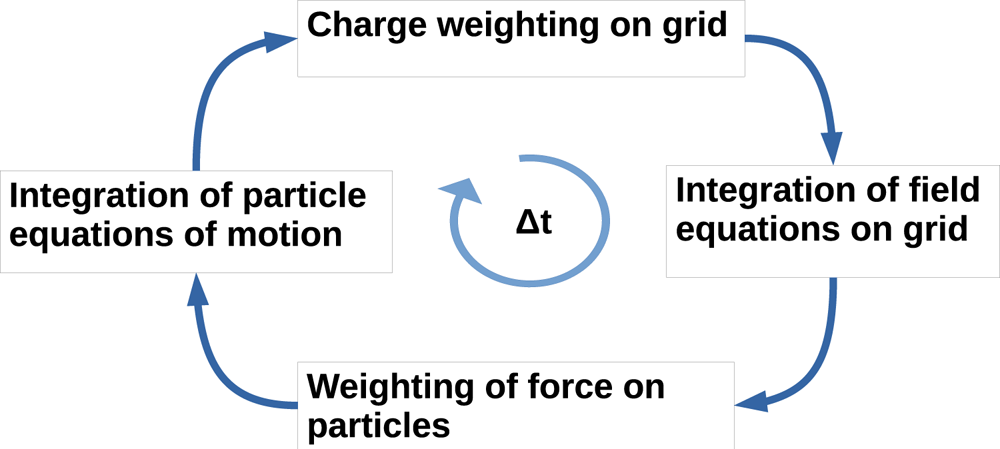
In the PIC method, the plasma is treated as an ensemble of computational particles (Dawson Reference Dawson1983; Birdsall & Langdon Reference Birdsall and Langdon2018; Hockney & Eastwood Reference Hockney and Eastwood2021). The computational particles move on the simulation domain, where, at every time iteration, the charge of each particle is distributed to a dedicated mesh. The charge is distributed according to particle positions by a linear interpolation scheme. Once the charge density $\rho$ is computed on the nodes of the mesh, the electric field $\boldsymbol {E}$
 can be integrated from the Poisson's equation. The full set of Maxwell equations has not been solved since the amount of RF power deposited outside the plasma source is a small fraction (usually less than 1 %) of the total power coupled to the plasma (Magarotto & Pavarin Reference Magarotto and Pavarin2020). This means that the propagation of RF waves in the plume is expected to have a minor influence on its dynamics. At the same time, currents (mainly azimuthal; Takahashi Reference Takahashi2019) induced by the presence of the magnetic nozzle are sufficiently low that the self-induced magnetic field produced can be neglected (errors less than 1 % are expected; Takahashi Reference Takahashi2019). Therefore the wave propagation in the plasma plume has been neglected and the magnetic field $\boldsymbol {B}$
 is static and equal to that imposed by the presence of the magnetic nozzle (Magarotto et al. Reference Magarotto, Melazzi and Pavarin2020b). Consequently, the Maxwell equations reduce to the Poisson equation:

with $\phi$ the electrostatic potential and $\boldsymbol {E} = -\boldsymbol {\nabla } \phi$
 . The Poisson equation is solved via a finite element method with a preconditioned conjugate algorithm to obtain $\phi$
 and consequently the field $\boldsymbol {E}$
 (Rogier & Volpert Reference Rogier and Volpert2021).
The force $\boldsymbol {F_p}$ acting on every particle is given by Lorenz force:

where $\boldsymbol {v_p}$ is the speed of the particle and $q_p$
 its charge. Force $\boldsymbol {F_p}$
 is computed interpolating fields on the position of each particle, and the associated trajectory is then integrated via a Runge–Kutta Cash–Karp method (Sarrailh et al. Reference Sarrailh, Mateo-Velez, Hess, Roussel, Thiebault, Forest, Jeanty-Ruard, Hilgers, Rodgers and Cipriani2015). This sequence of operations is repeated at each time iteration (see figure 2), self-consistently evolving the particles and the electric field states. The simulations are performed until steady state is reached.
Time loop in PIC code.
It is worth noting that the Runge–Kutta Cash–Karp method shows a considerable propagation of numerical error integrating the trajectory of a charged particle (Qin et al. Reference Qin, Zhang, Xiao, Liu, Sun and Tang2013). A correction factor in the pusher algorithm has been added to reduce the energy numerical drift.
Finally, the effect of collisions has been neglected. This approach is proven to provide a valuable preliminary insight on the dynamics of the plume for typical operation conditions of MEPTs (Martinez-Sanchez et al. Reference Martinez-Sanchez, Navarro-Cavallé and Ahedo2015). Nonetheless collisions will be implemented in future works to estimate quantitatively the influence that phenomena such as the doubly trapped electrons have on the plume. The latter in fact are produced by collisional effects (Zhou et al. Reference Zhou, Sánchez-Arriaga and Ahedo2021).
2.2. Boundary conditions
The simulation domain and the boundary surfaces are represented in figure 3. The boundary conditions that have been imposed for the closure of (2.1) are the following.
(i) Dirichlet condition on the surfaces of the spacecraft, i.e.
(2.3)\begin{equation} \phi = \begin{cases} \phi_o, & \text{ on the thruster outlet surface (particle source)},\\ 0, & \text{ on other surfaces}. \end{cases} \end{equation}
(ii) Robin condition on the external boundary (Thiebault et al. Reference Thiebault, Jeanty-Ruard, Souquet, Forest, Mateo-Velez, Sarrailh, Rodgers, Hilger, Cipriani and Payan2015):
(2.4)\begin{equation} \frac{\textrm{d}\phi}{\textrm{d}\boldsymbol{k}} +\frac{\boldsymbol{r} \cdot\boldsymbol{k}}{r^2}\phi = 0, \end{equation}with $\boldsymbol{k}$ the external normal to the surface and $\boldsymbol{r}$ the vector going from the geometric centre of the particle source to the external boundary surface. Equation (2.4) derives from the assumption that at infinity $\phi =0$ and that $\phi \propto 1/r$ (Thiebault et al. Reference Thiebault, Jeanty-Ruard, Souquet, Forest, Mateo-Velez, Sarrailh, Rodgers, Hilger, Cipriani and Payan2015).


Simulation domain: the boundary surfaces are coloured in brown, the particle source in green. The simulation domain corresponds to the grey zone.

As far as particle motion is concerned, the definition of an electron energy boundary condition is required to simulate properly the dynamics of the plasma plume (Li et al. Reference Li, Merino, Ahedo and Tang2019). Indeed, to maintain the current-free condition (Takahashi Reference Takahashi2019), a positive potential drop occurs between the thruster outlet and ‘infinity’. The simulation should take into account the electrons that do not have enough kinetic energy to escape this potential drop and therefore return to the plasma source or become trapped in the plume. This is fundamental also from a computational standpoint to avoid the so-called ‘numerical pump instability’ (Brieda Reference Brieda2005). Despite the finite computational domain dimensions, these trapped electrons can be taken into account by adding an energy-based boundary condition. Energy $E_{\textrm {tot}}$ denotes the total energy of the electrons at the external boundary:

with $m_p$ the mass of the particle and $\phi _b$
 the external boundary potential. Electrons that reach the external boundary surfaces with a negative $E_{\textrm {tot}}$
 are reflected specularly; in contrast, electrons with a positive $E_{\textrm {tot}}$
 are absorbed. In fact the former do not have enough energy to achieve infinity with $|v_p|\geq 0$
 . Ions that reach the external boundary are absorbed. Ions and electrons that reach the surfaces of the spacecraft, including the thruster outlet surface, are absorbed too.
2.3. Particle sources
The computational particles are ejected from the surface of the thruster named ‘thruster outlet’ in figure 3. Hereafter, an $xyz$ Cartesian coordinate system with the $z$
 axis normal to the thruster outlet is considered; $z$
 is also the axis of symmetry for the computational domain. As detailed in §§ 2.3.1 and 2.3.2, a Maxwellian distribution function is assumed for all the species at the thruster outlet. This hypothesis is justified by the value of the plasma density which is orders of magnitude higher in the production stage than in the plume, so a thermodynamic equilibrium is more likely (Cichocki et al. Reference Cichocki, Domínguez-Vázquez, Merino and Ahedo2017; Li et al. Reference Li, Merino, Ahedo and Tang2019; Magarotto & Pavarin Reference Magarotto and Pavarin2020; Magarotto et al. Reference Magarotto, Manente, Trezzolani and Pavarin2020a). Moreover, the assumption of a Maxwellian distribution function at the thruster outlet is supported by experiments performed on helicon sources (Chen & Blackwell Reference Chen and Blackwell1999). Hereafter, random variables are written in upper case, and particular realizations of such variables are written in the corresponding lower case.
2.3.1. Electron source
The speed $V_x$ along the $x$
 axis and the speed $V_y$
 along the $y$
 axis of the ejected electrons are random variables that follow a normal distribution of mean $\mu = 0$
 and standard deviation $\sigma$
 given by

with $T_e$ the electron temperature expressed in kelvin, $k_B$
 the Boltzmann constant and $m$
 the electron mass. The speed along the $z$
 axis $V_z$
 of the ejected electrons has the following probability density function (Li et al. Reference Li, Merino, Ahedo and Tang2019):

Equation (2.7) represents a flux of electrons ejected from the thruster outlet with a Maxwellian distribution function. Instead the flux of electrons returning at the same surface ($v_z<0$ ) is an output of the simulation that cannot be imposed a priori. It is easy to show that the norm of the speed of the ejected electrons, denoted as $V$
 , reads (Bartsch Reference Bartsch2014)

In particular, from the definition of electron current (Chen et al. Reference Chen1984), it is possible to compute the electron density $n_e$ at the thruster outlet as

with $e$ the electron charge, $S$
 the surface area of the thruster outlet, $I_e$
 the electron net current at the thruster outlet and $|E[\widetilde {V_z}]|$
 the expected value of the electron speed $\widetilde {V_z}$
 at the thruster outlet. The electron speed $\widetilde {V_z}$
 at the thruster outlet corresponds to electrons both ejected and absorbed at this surface.
2.3.2. Ion source
Ions are ejected from the thruster outlet with the following velocities:

where $V_n$ is a random variable that follows a normal distribution of mean $\mu = 0$
 and standard deviation $\sigma$
 given by

with $T_i$ the ion temperature, $M$
 the ion mass and $u_B$
 the Bohm speed:

Here $\varTheta$ is a random variable that follows a continuous uniform distribution in the interval $[0, \theta _t ]$
 . Angle $\theta _t$
 corresponds to the nozzle divergence angle (see figure 3). It is associated with the presence of a conical source (Charles, Boswell & Takahashi Reference Charles, Boswell and Takahashi2013) or an expansion nozzle (Manente et al. Reference Manente, Trezzolani, Magarotto, Fantino, Selmo, Bellomo, Toson and Pavarin2019). Considering typical MEPTs, in this study the assumption $\theta _t < 45^{\circ }$
 has been made (Bellomo et al. Reference Bellomo, Di Fede, Magarotto, Manente, Pavarin, Trezzolani, Selmo, De Carlo, Toson and Minute2021). Parameter $\varLambda$
 is a random variable that follows a continuous uniform distribution in the interval $[0, 2{\rm \pi} ]$
 . The expected value $E[V_z]$
 and the variance $\textrm {Var}[V_z]$
 of $V_z$
 are
are


In typical MEPT configurations the plasma is mesothermal (i.e. $T_e \gg T_i$ ) (Balkey et al. Reference Balkey, Boivin, Kline and Scime2001); therefore $u_B$
 is higher than $\sigma$
 and it is reasonable to assume that

where $P(V_z < 0)$ is the probability that ions are ejected with a negative $v_z$
 . The ion density $n_i$
 at the thruster outlet can be computed as

with $q_i$ the ion charge, $I_i$
 the ion net current at the thruster outlet and $E[\widetilde {V_z}|$
 the expected value of ion speed $\widetilde {V_z}$
 at the thruster outlet. The ion speed $\widetilde {V_z}$
 at the thruster outlet is the speed corresponding to ions both ejected and absorbed by the thruster outlet. The outlet potential $\phi _o$
 is larger than the boundary potential $\phi _b$
 ; therefore a negligible amount of ions return to the thruster outlet and it is reasonable to assume that $\widetilde {V_z} \approx V_z$
 .
.
2.4. Control loop
For the sake of simplicity hereafter, it has been considered that the ion population is composed of only one species. Considering typical operating conditions of MEPTs, this assumption is reasonable where the thruster is operated with noble gases (Chabert et al. Reference Chabert, Arancibia Monreal, Bredin, Popelier and Aanesland2012; Lafleur Reference Lafleur2014). Regardless, the following control strategy can be easily generalized if several ion species are considered. With the focus of this work on MEPTs, the current-free condition has been imposed at the thruster outlet (Manente et al. Reference Manente, Trezzolani, Magarotto, Fantino, Selmo, Bellomo, Toson and Pavarin2019). It is worth noting that this condition is truly respected only ‘on average’ since RF wave propagation can induce instantaneous non-null currents. However, this effect is expected to influence mildly the plume dynamics and, in particular, the computation of macroscopic quantities for the propulsive performance. In fact, the RF power deposited outside the source is expected to be only 1 % of the total (Magarotto & Pavarin Reference Magarotto and Pavarin2020). The current-free condition at the thruster outlet can be expressed as

If quasi-neutrality holds true, from (2.9) and (2.16):


Assuming $\widetilde {V_z} \approx V_z$ , from (2.13) and (2.19):

The term $|E[\widetilde {V_{z,e}}]|$ being highly nonlinear dependent on the boundary conditions at the thruster outlet (Martinez-Sanchez et al. Reference Martinez-Sanchez, Navarro-Cavallé and Ahedo2015), any noise or deviation from analytical behaviour could lead to a condition that strongly departs from current-free and quasi-neutrality. Consequently, a control loop is needed to reach the steady state while ensuring these conditions (Li et al. Reference Li, Merino, Ahedo and Tang2019).
The loop controls the parameters that mainly drive the simulation, namely the potential at the thruster outlet $\phi _o$ , along with the electron and ion currents injected into the domain ($I_e^+$
 and $I_i^+$
 respectively). From (2.15), $I_i^+$
 is assumed constant during the simulation and is given by

with $\dot {m}$ the propellant mass flow rate. To achieve the current-free condition at the steady state, for every time step $t$
 the potential at the thruster outlet ($\phi _o^t$
 ) is updated according to the explicit relation

with $I_e^{t-1}$ and $I_i^{t-1}$
 respectively the electron and ion net currents at the thruster outlet at the previous time step and $k_1$
 a positive control coefficient. To achieve quasi-neutrality at the steady state, for every time step the emitted electron current (${I_e^+}^t$
 ) is updated according to the explicit relation

where ion and electron densities are computed at the thruster outlet and $k_2$ is a positive control coefficient. It is worth noting that, according to (2.9), $n_e$
 depends on both $I_e^+$
 and $I_e^-$
 , the latter being the absorbed electron current that cannot be imposed directly as an input of the simulation since it is driven by $\phi _o$
 . Namely (2.22) and (2.23) impose a self-consistent relation between $\phi _o$
 , $I_e^+$
 and $I_i^+$
 to enforce current-free and quasi-neutrality conditions.
At the first time step, the quantities $\phi _o$ and $I_e^+$
 are imposed according to the analytical values derived in Appendix A for a non-magnetized case, and then updated according to (2.22) and (2.23) up to the achievement of the steady-state condition (see § 2.5). As a result, the simulation provides as an output also the self-consistent value of the total potential drop across the plume (i.e. $\phi _o$
 ) which depends on the geometry of the system and the imposed flow of propellant.
2.5. Time loop termination
A simulation is assumed to be at the steady state if the number of particles leaving through the external boundaries matches the number of new particles introduced into the system by the source. This condition is met for a sufficiently high number of time steps ($\alpha$ ) in order to avoid a ‘false positive’ induced by PIC noise. Specifically, the steady-state condition is implemented by requiring that (Gallina et al. Reference Gallina, Magarotto, Manente and Pavarin2019)

where $\nu$ is a user-defined number that represents a steady-state condition (usually $\nu \sim 10^{-4}$
 ), $N^t_{\textrm {sp}}$
 is the number of super-particles in the system at time step $t$
 and $h$
 is the current time step. As a rule of thumb, $\alpha \sim 50$
 has been assumed.
2.6. Performance indicators
The thrust $F$ produced by the thruster is obtained by summing, for each species $p$
 , the contribution due to the momentum exchange and to the pressure. Specifically it is computed with (Zhou et al. Reference Zhou, Pérez-Grande, Fajardo and Ahedo2019)

with $S_b$ the external boundary surface, $\boldsymbol {k}$
 the external normal to the surface and $\boldsymbol {\hat {z}}$
 the unity vector parallel to the $z$
 axis. The specific impulse is obtained by

with $g_0$ the standard gravity.
3. Code verification
A cross-validation of the methodology has been done with Starfish, a two-dimensional open-source PIC software; for this specific validation, all the electrons that reach the external boundary are absorbed. The other hypotheses are consistent with the methodology described in § 2. The computational domain chosen for the cross-validation (see figure 4) consists of a cylinder of radius 8 cm and height 16 cm; the spacecraft is represented by a cylinder of radius 5 cm and height 1 cm. The thruster outlet is a circle of radius 2 cm and centre placed on the axis of symmetry at coordinate $z$ = 2 cm. The two codes have been compared in the absence of a magnetic field. This is consistent with the scope of the verification since boundary conditions, particle sources and the control loop do not depend directly on the magnetic field (see § 2). Moreover, in this condition the comparison between a three-dimensional and a two-dimensional code is more straightforward since azimuthal dynamics (e.g. currents induced by the diamagnetic drift; Takahashi Reference Takahashi2019) is expected to be negligible. Xenon propellant has been simulated, with operating conditions consistent with a MEPT operated at 10 W input power and the pressure in the discharge chamber is assumed of the order of 0.1 Pa (Bellomo et al. Reference Bellomo, Di Fede, Magarotto, Manente, Pavarin, Trezzolani, Selmo, De Carlo, Toson and Minute2021).

Figure 5 shows the ion density ($n_i$ ), the plasma potential ($\phi$
 ) and the ion speed ($V_i$
 ) along the $z$
 axis of the computational domain. The difference between the results provided by SPIS and Starfish is denoted $n_i^{\textrm {bias}}$
 , $\phi ^{\textrm {bias}}$
 and $V_i^{\textrm {bias}}$
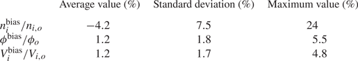
 for ion density, plasma potential and ion speed respectively. Table 1 shows the corresponding average value, standard deviation and maximum value adimensionalized with respect to $n_{i, o}$
 , $\phi _o$
 and $V_{i, o}$
 , namely the same quantities evaluated at the thruster outlet. The results of SPIS and Starfish show a very good agreement regarding the plasma potential and the ion speed (differences $\lesssim$
 5 %). Regarding the ion density there is a larger bias, in any case comparable with the PIC noise. The coarser mesh used for the three-dimensional simulation (with respect to the two-dimensional one used for Starfish) is a possible explanation of this bias.
Comparison between the results of SPIS (solid line) and Starfish (dashed line). Ion density $n_i$ (a), plasma potential $\phi$
 (b) and ion speed $|V_i|$
 (c) are depicted along the $z$
 axis.
axis.

Difference between the results provided by SPIS and Starfish for ion density, plasma potential and ion speed. Average value, standard deviation and maximum value are reported adimensionalized by the corresponding value at the thruster outlet position.
4. Results
The SPIS code has been applied to simulate the plume of a MEPT adopting the methodology presented in § 2, and using the computational domain depicted in figure 4. Xenon propellant has been considered and the input values are consistent with the operating conditions of a MEPT operated at 50 W input power (Bellomo et al. Reference Bellomo, Di Fede, Magarotto, Manente, Pavarin, Trezzolani, Selmo, De Carlo, Toson and Minute2021), namely ion mass flow rate $\dot {m}=0.05\, \textrm {mg}\,\textrm {s}^{-1}$ and electron temperature $T_e = 3\, \textrm {eV}$
 . Only singly charged ions (Xe$^+$
 ) have been simulated since the doubly charged population (Xe$^{2+}$
 ) is negligible for a discharge with $T_e < 10$
 eV (Chabert et al. Reference Chabert, Arancibia Monreal, Bredin, Popelier and Aanesland2012; Souhair et al. Reference Souhair, Magarotto, Majorana, Ponti and Pavarin2021). Hereafter $\tilde {B}$
 denotes the average value of the magnetic field at the thruster outlet. Two configurations have been compared: (i) $\tilde {B} = 0\, \textrm {G}$
 (absence of magnetic field) and (ii) $\tilde {B} = 300\, \textrm {G}$
 ; the magnetic field assumed in case (ii) is depicted in figure 6.
Scheme of the magnetic field adopted in the $\tilde {B} = 300$ G configuration.

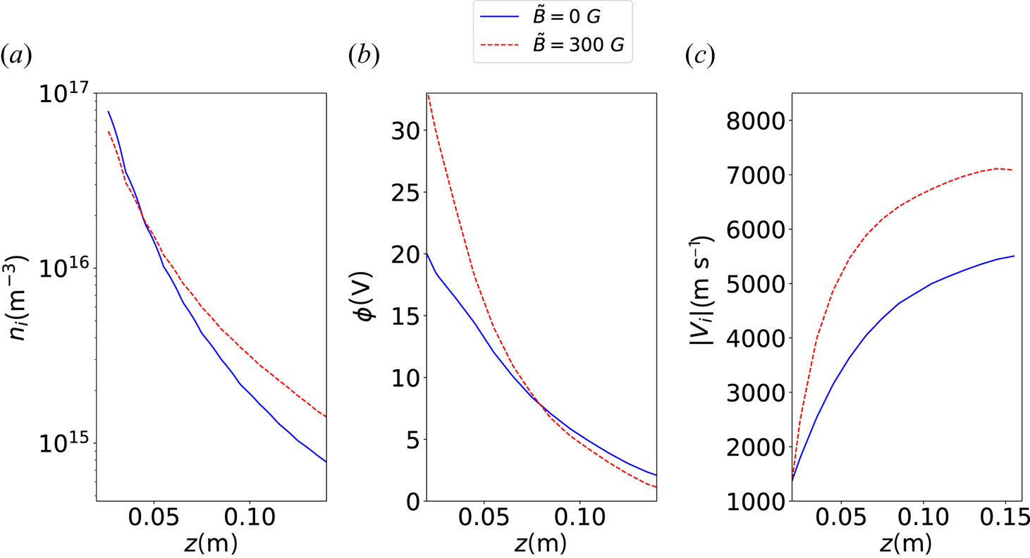
Figure 7 shows the plasma potential, the ion density and the ion speed along the $z$ axis of the computational domain. Figures 8 and 9 show the ion density and the ion speed on the $x$
 –$z$
–$z$ plane. Results on the $y$
 –$z$
–$z$ plane are not presented due to the axisymmetry of the domain. As depicted in figure 7(b), the potential at the thruster outlet $\phi _o$
 is equal to 20 V for $\tilde {B} = 0$
 G and 33 V for $\tilde {B} = 300$
 G. The increase in the potential drop in the presence of the magnetic nozzle was expected due to the increase of the ambipolar effect. The magnetized electrons are accelerated axially by the magnetic nozzle and therefore larger electric fields are necessary to maintain the quasi-neutrality and the current-free condition. This effect influences the overall dynamics of the plume.
(i) The presence of the magnetic field increases the ion speed by approximatively 40 % (see figures 7c and 9).
(ii) In the presence of the magnetic nozzle, ions are strongly accelerated near the thruster, reaching approximately their maximum speed at $z = 10$
cm (see figures 7c and 9).(iii) The magnetic field changes the plume's shape (see figures 7a and 8). In the $\tilde {B} = 0$
G configuration some ions have negative axial speed and reach the external boundary at $z = 0$ cm. The magnetic topology considered in the $\tilde {B} = 300$ G configuration facilitates avoidance of this negative ion flux and therefore reduces the plume divergence angle. It is worth noting that other magnetic nozzle configurations, for example fields with excessively steep gradients, might instead increase the divergence angle of the plume.


Comparison between the results with $\tilde {B} = 0$ G (solid line) and $\tilde {B} = 300$
 G (dashed line). Ion density $n_i$
 (a), plasma potential $\phi$
 (b) and ion speed $|V_i|$
 (c) are depicted along the $z$
 axis.
axis.
Ion density $n_i$ on the $x$
 –$z$
–$z$ plane; comparison between the results with $\tilde {B} = 0$
 G (a) and $\tilde {B} = 300$
 G (b).

Ion speed $|V_i|$ on the $x$
 –$z$
–$z$ plane; comparison between the results with $\tilde {B} = 0$
 G (a) and $\tilde {B} = 300$
 G (b).

The presence of the magnetic field improves the propulsive performance of the thruster; $I_{\textrm {sp}}$ increases from 260 s up to 610 s if $\tilde {B} = 300$
 G. Moreover, in table 2 the specific impulse obtained from the numerical simulation and that measured in a test campaign are compared (Bellomo et al. Reference Bellomo, Di Fede, Magarotto, Manente, Pavarin, Trezzolani, Selmo, De Carlo, Toson and Minute2021). In spite of the remarkably good quantitative agreement it is worth highlighting that this is not intended to be a proper experimental validation but only a preliminary check of the numerical results.
Specific impulse obtained from numerical simulation and that obtained from test campaign.

The consistency of the numerical results has been checked analysing the steady-state values of $\phi _o$ and $I_e^+$
 computed for $\tilde {B} = 0$
 G. In fact, the initial values assumed according to (A9) and (A6) are expected to be almost equal to the values at the steady state since calculations performed in Appendix A refer to a non-magnetized plume. Initial values are $\phi _o^0 = 19.4$
 V and $|{I_e^+}^0| = 211 I_i^+$
 ; at the steady state $\phi _o = 20.0$
 V and $|I_e^+| = 310 I_i^+$
 . A good agreement is found as far as the potential drop is concerned; in contrast, $|I_e^+|$
 is higher than the value predicted in theory. The latter difference can be considered acceptable bearing in mind the highly nonlinear terms of (A6). This bias in $|I_e^+|$
 is associated with the lower potential drop predicted by (A9) and with the numerical noise. The robustness of the methodology proposed in § 2 is therefore evidenced by the accordance between values obtained via the control loop and the theoretical model presented in Appendix A.
Figure 10 shows the trajectories of the electrons and their kinetic energy for $\tilde {B} = 0\,\textrm {G}$ and $\tilde {B} = 300\,\textrm {G}$
 . In the absence of a magnetic field, the motion of the electrons is chaotic, consistent with the assumption of a Maxwellian velocity distribution function at the thruster outlet. Instead, in the magnetized case, electrons describe a gyrating motion in proximity of the thruster outlet. Closer to the outer boundary, where the intensity of the magnetic field is lower, electrons are no longer frozen to field lines and this results in a disordered motion.
Trajectory of electrons on the computational domain and their kinetic energy; comparison between the results with $\tilde {B} = 0\,\textrm {G}$ (a) and $\tilde {B} = 300\,\textrm {G}$
 (b).
(b).

5. Conclusion
A three-dimensional fully kinetic PIC strategy has been implemented to simulate the plume of a magnetically enhanced plasma thruster. The approach proposed is promising: results are coherent with experimental data (Bellomo et al. Reference Bellomo, Di Fede, Magarotto, Manente, Pavarin, Trezzolani, Selmo, De Carlo, Toson and Minute2021) and show the reduction of the plume divergence angle, the increase of ion speed and the increase of the specific impulse for the magnetic nozzle configuration examined in the study. The control loop implemented permits the enforcement of the quasi-neutrality and the current-free conditions. In addition, the robustness of the methodology proposed in § 2 is also sustained by the good accordance of the values obtained by the control loop with the theoretical values presented in Appendix A.
Nonetheless, the model needs further improvements: a correction factor in the pusher algorithm has been added to reduce the energy numerical drift, but the Boris algorithm (Zenitani & Umeda Reference Zenitani and Umeda2018) remains the preferable integration method for advancing a charged particle and it will be adopted for future simulations. Additionally, the domain of the simulation should be extended inside the thruster, in the region corresponding to the physical nozzle where, due to the high plasma density, collisions cannot be neglected. This improvement will permit the quantitative estimation and characterization of phenomena, such as doubly trapped electrons, which require including collisions into the model. Finally, a complete experimental campaign (Trezzolani et al. Reference Trezzolani, Magarotto, Manente and Pavarin2018) will be done to validate the numerical results.
Acknowledgements
Editor Cary Forest thanks the referees for their advice in evaluating this article.
Funding
The authors are grateful for the contributions of ‘University of Padova Strategic Research Infrastructure Grant 2017: CAPRI: Calcolo ad Alte Prestazioni per la Ricerca e l'Innovazione’ to this study.
Declaration of interests
The authors report no conflict of interest.
Author contributions
S.D.F., M.M. and S.A. derived the theory. S.D.F. and M.M. wrote the paper. S.D.F. and S.A. developed the code and performed the simulations respectively with SPIS and Starfish. D.P. supervised the research.
Appendix A
This appendix describes the hypothesis considered to compute $\phi _o^0$ and ${I_e^+}^0$
 , i.e. the initial parameters of (2.22) and (2.23). The appendix gives also the analytical solution of $\phi _o$
 and ${I_e^+}$
 in the case of a steady-state collisionless unmagnetized expansion.
The hypotheses for the computation of ${I_e^+}^0$ are current-free condition, steady-state condition, $E_{\textrm {tot}}$
 conservation and the absence of a magnetic field. In steady-state condition:

with $I_{e, b}$ the electron current absorbed at the external boundary and $I_{e, o}$
 the total electron current at the thruster outlet. In the absence of a magnetic field, electrons come back to the thruster outlet only if their total energy is negative. Therefore, due to $E_{\textrm {tot}}$
 conservation, from (A1):

with $P(E_{\textrm {tot}}>0)$ the probability that electrons have a positive total energy. If current-free condition holds and if ions do not come back to the thruster outlet, (A2) becomes

If the potential $\phi _o$ is constant along the surfaces of the thruster outlet:

If the speed of the ejected electrons follows a Maxwellian distribution, (A4) becomes

Equation (A5) shows the probability that electrons have a positive total energy in the case of a Maxwellian source distribution, particle energy conservation and the absence of a magnetic field. It is clear that the relation between the outlet potential and the probability that electrons come back to the particle source is highly nonlinear; consequently also $|E[\widetilde {V_{z,e}}]|$ depends highly nonlinearly on $\phi _o$
 . From (A3) and (A5):

Here $\phi _o^0$ is computed with the additional hypothesis that close to the thruster outlet the electron distribution remains Maxwellian after the ejection. Due to the high plasma density near the thruster outlet, this hypothesis is reasonable in the absence of a magnetic field. Therefore it can be assumed that

Combining (A7), (2.9) and (A2) :

Combining (A8), (A5) and (2.20) :

Potential $\phi _o^0$ is obtained solving numerically (A9); ${I_e^+}^0$
 is therefore obtained with (A6). As discussed in § 4, $\phi _o$
 obtained by the control loop in the absence of a magnetic field is very close (0.6 V lower, difference $\approx$
 3 %) to the value obtained by (A9). The value of ${I_e^+}^0$
 obtained by (A6) is 33 % lower than that obtained by the control loop. This difference can be considered acceptable bearing in mind the highly nonlinear terms of (A6). The bias is due to a lower potential drop predicted by (A9) and numerical noise. Therefore the good agreement between theoretical values and values obtained by the control loop supports the validity of the hypotheses presented in this appendix.


 Open access