


1. Background
The collective behaviour of schooling fish is not only visually striking, it also presents a complex interplay of hydrodynamics, ethology and environmental adaptation. Schooling and collective swimming provide several advantages, including improved foraging efficiency (Pitcher, Magurran & Winfield Reference Pitcher, Magurran and Winfield1982; Pavlov & Kasumyan Reference Pavlov and Kasumyan2000), predator avoidance (Shaw Reference Shaw1962; Pavlov & Kasumyan Reference Pavlov and Kasumyan2000; Larsson Reference Larsson2012), stealth (Zhou, Seo & Mittal Reference Zhou, Seo and Mittal2024) and, notably, hydrodynamic efficiency (Weihs Reference Weihs1973; Partridge & Pitcher Reference Partridge and Pitcher1979; Pavlov & Kasumyan Reference Pavlov and Kasumyan2000; Zhou, Seo & Mittal Reference Zhou, Seo and Mittal2023). The improvement in swimming efficiency has garnered significant attention for its implications for energy conservation during locomotion (Weihs Reference Weihs1973; Pavlov & Kasumyan Reference Pavlov and Kasumyan2000; Liao Reference Liao2007; Timm, Pandhare & Masoud Reference Timm, Pandhare and Masoud2024). Recent studies have also explored simplified modelling approaches to systematically quantify and map energetic benefits across different swimmer configurations, providing practical insights into wake interactions and collective swimming energetics (Heydari, Hang & Kanso Reference Heydari, Hang and Kanso2024). Specifically, fish within a school can harness the vortices generated by other fish, thereby reducing their energy expenditure (Taguchi & Liao Reference Taguchi and Liao2011; Verma, Novati & Koumoutsakos Reference Verma, Novati and Koumoutsakos2018; Li et al. Reference Li, Nagy, Graving, Bak-Coleman, Xie and Couzin2020; Seo & Mittal Reference Seo and Mittal2022; Guo et al. Reference Guo, Han, Zhang, Wang, Lauder, Di Santo and Dong2023; Ormonde et al. Reference Ormonde, Kurt, Mivehchi and Moored2024). This phenomenon has driven extensive research into the spatial configurations, tailbeat synchronisation and flow dynamics that govern schooling behaviour (Partridge et al. Reference Partridge, Pitcher, Cullen and Wilson1980; Maertens, Gao & Triantafyllou Reference Maertens, Gao and Triantafyllou2017; Verma et al. Reference Verma, Novati and Koumoutsakos2018; Seo & Mittal Reference Seo and Mittal2022; Pan & Lauder Reference Pan and Lauder2024).
The study of fish schooling has advanced significantly in recent decades, moving from foundational qualitative observations (Weihs Reference Weihs1973; Partridge & Pitcher Reference Partridge and Pitcher1979; Partridge et al. Reference Partridge, Pitcher, Cullen and Wilson1980) to sophisticated experimental (Shaw Reference Shaw1962; Abrahams & Colgan Reference Abrahams and Colgan1985; Becker et al. Reference Becker, Masoud, Newbolt, Shelley and Ristroph2015; Marras et al. Reference Marras, Killen, Lindström, McKenzie, Steffensen and Domenici2015; Ashraf et al. Reference Ashraf, Godoy-Diana, Halloy, Collignon and Thiria2016; Newbolt, Zhang & Ristroph Reference Newbolt, Zhang and Ristroph2019; McKee et al. Reference McKee, Soto, Chen and McHenry2020; Wei et al. Reference Wei, Hu, Zhang and Zeng2022; Zhang et al. Reference Zhang, Ko, Calicchia, Ni, Lauder and Hedenström2024) and computational (Maertens et al. Reference Maertens, Gao and Triantafyllou2017; Verma et al. Reference Verma, Novati and Koumoutsakos2018; Hang et al. Reference Hang, Heydari, Costello and Kanso2022; Seo & Mittal Reference Seo and Mittal2022; Zhou, Seo & Mittal Reference Zhou, Seo and Mittal2022; Gungor, Khalid & Hemmati Reference Gungor, Khalid and Hemmati2024; Pan et al. Reference Pan, Zhang, Kelly and Dong2024; Zhou et al. Reference Zhou, Seo and Mittal2024; Zhou, Seo & Mittal Reference Zhou, Seo and Mittal2025) investigations. Early studies focused primarily on observable patterns and school formations, offering limited insights into the intricate fluid mechanics at play. However, advances in experimental techniques and computational fluid dynamics (CFD) have enabled researchers to quantify these hydrodynamic effects, revealing the intricate interactions between individual fish and the surrounding flow. These developments have been crucial in identifying the potential for energy savings and performance enhancement through schooling interactions, especially in carangiform swimmers (Pavlov & Kasumyan Reference Pavlov and Kasumyan2000; Liao Reference Liao2007; Li et al. Reference Li, Kolomenskiy, Liu, Thiria, Godoy-Diana and Gurka2019; Seo & Mittal Reference Seo and Mittal2022; Timm et al. Reference Timm, Pandhare and Masoud2024).
1.1. Knowledge gap and current contribution
Despite these advances, obtaining precise measurements of the flow fields generated by individual fish within a school remains challenging. Fish within schools move unpredictably, making it difficult to control their positions or gather detailed fluid dynamic data at the individual swimmer level. Consequently, many experimental studies (Herskin & Steffensen Reference Herskin and Steffensen1998; Cooke, Thorstad & Hinch Reference Cooke, Thorstad and Hinch2004; Taguchi & Liao Reference Taguchi and Liao2011; Zhang et al. Reference Zhang, Ko, Calicchia, Ni, Lauder and Hedenström2024) focus on quantifying the metabolic costs of groups of fish, successfully capturing the phenomenon of energy savings but falling short of uncovering the precise mechanisms that drive it, thus limiting translational applications. Computational flow modelling studies (Verma et al. Reference Verma, Novati and Koumoutsakos2018; Seo & Mittal Reference Seo and Mittal2022; Pan et al. Reference Pan, Zhang, Kelly and Dong2024) have achieved three-dimensional, high-fidelity reconstructions of fish schooling flow fields, yet these models are constrained by the substantial computational costs associated with simulating large, complex fish schools over time. High-fidelity simulations require extensive computational resources, often relying on supercomputers. Additionally, in CFD simulations, fish position is typically prescribed and as the number of swimmers increases, the possible configurations for fish in a school expand rapidly. As a result, CFD studies are often limited to small groups or simplified models, which cannot fully capture the complex dynamics of real-world schooling behaviour. In particular, while CFD models have examined simple, highly regular configurations, such configurations are hardly ever observed in real fish schools. While this could be due to factors in schooling other than hydrodynamic performance, this could also be a reflection of the fact that the ‘landscape’ of improved thrust performance in schools is vastly more complicated than indicated by CFD studies that have only explored a limited range of possible school topologies.
To address these experimental and computational challenges, in this study, we propose a leading-edge vortex-based model (LEVBM) that leverages insights from solitary fish studies and flapping foil models to predict the hydrodynamic performance of trailing fish in a school. Our prior studies (Seo & Mittal Reference Seo and Mittal2022; Zhou et al. Reference Zhou, Seo and Mittal2024) have demonstrated the critical role of leading-edge vortices (LEVs) in the thrust generation of individual fish, particularly in the context of caudal fin dynamics (details in the next section). In parallel studies, we have validated the LEVBM for thrust generation from flapping foils (Raut, Seo & Mittal Reference Raut, Seo and Mittal2024) and shown that the LEVBM can be used to guide the relative placement of foils in multifoil propulsors so as to maximise the gains in thrust generated from the hydrodynamic interactions between the foils (Raut, Seo & Mittal Reference Raut, Seo and Mittal2025).
In the current study, we extend this idea to ‘carangiform’ body-caudal fin (BCF) swimmers, fish or fish-like swimmers that use an undulatory motion of their body and caudal fin. The LEVBM uses pre-simulated wake flow fields from a leading fish and the tailbeat kinematics of the trailing fish to evaluate the potential thrust generation of the trailing fish placed in the wake of the leading fish, without employing additional high-fidelity simulations. This enables us explore a wide parameter space, including relative position, tailbeat phase, amplitude, Reynolds number and number of fish, and gain new insights into the hydrodynamic implications for coordinated swimming in these BCF swimmers.
2. Methods
2.1. Leading-edge vortex-based model for thrust generation
In our previous study (Raut et al. Reference Raut, Seo and Mittal2024), we have proposed a model to predict thrust generation by a pitching and heaving foil based on its kinematics. Given that the caudal fin of BCF swimmers functions similarly to a pitching and heaving foil, this model can also be applied to predict the thrust generation by the caudal fin.
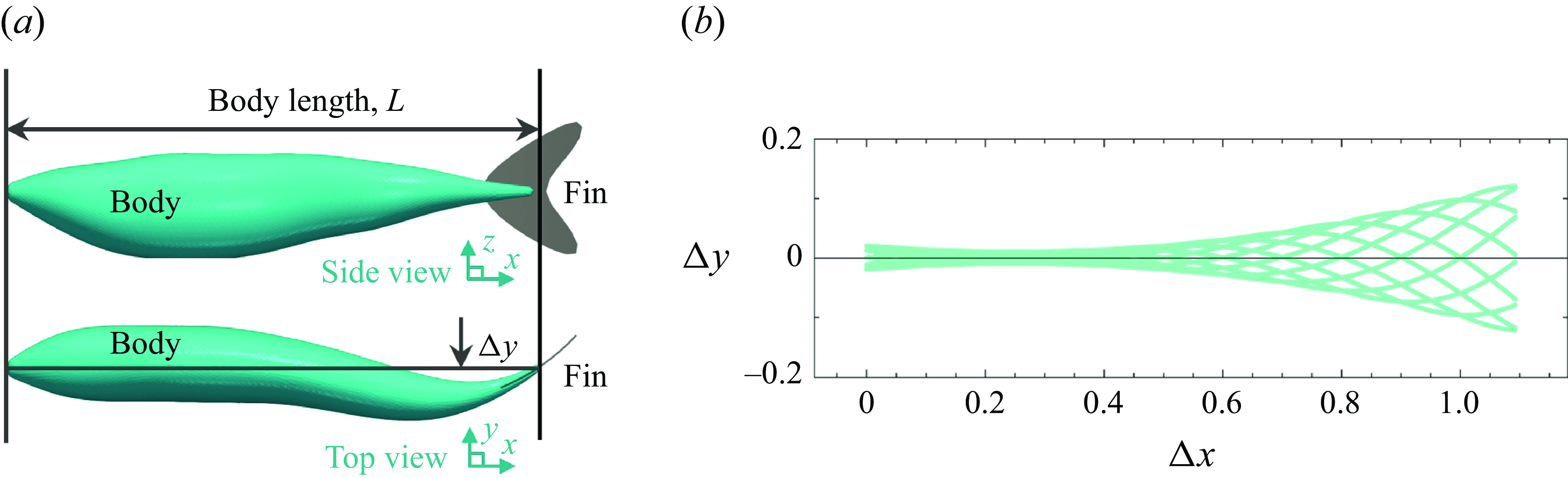
The swimming kinematics of the current BCF swimmer, shown in figure 1, are given by the following equation:
 \begin{equation} \Delta y (x) = A(x ) \sin (kx - 2 \pi ft ); \quad A(x)/L = a_0 +a_1(x/L)+a_2(x/L)^2, \end{equation}
Three-dimensional model and centreline kinematics of a solitary fish. (a) Side and top views of the simulated fish, showing the body and caudal fin. (b) Lateral displacement of the fish centreline over one tailbeat cycle, $\Delta t = T/10$
, where T is the tailbeat time period, illustrating the kinematic motion along the axial length,
$\Delta t = T/10$
, where T is the tailbeat time period, illustrating the kinematic motion along the axial length, $\Delta x$
.
$\Delta x$
.
where $\Delta y(x)$
is the lateral displacement,
$\Delta y(x)$
is the lateral displacement, $L$
is the body length,
$L$
is the body length, $x$
is the axial distance from the nose,
$x$
is the axial distance from the nose, $f$
is the tailbeat frequency and
$f$
is the tailbeat frequency and $A(x)$
is the amplitude modulation function. Based on the literature (Videler & Hess Reference Videler and Hess1984) and our previous studies (Seo & Mittal Reference Seo and Mittal2022; Zhou et al. Reference Zhou, Seo and Mittal2024), the parameters are set as
$A(x)$
is the amplitude modulation function. Based on the literature (Videler & Hess Reference Videler and Hess1984) and our previous studies (Seo & Mittal Reference Seo and Mittal2022; Zhou et al. Reference Zhou, Seo and Mittal2024), the parameters are set as $k=2\pi /L$
,
$k=2\pi /L$
, $a_0=0.02$
,
$a_0=0.02$
, $a_1=-0.08$
and
$a_1=-0.08$
and $a_2=0.16$
. Based on these kinematics, the heaving (
$a_2=0.16$
. Based on these kinematics, the heaving ( $h(t)$
) and pitching motion (
$h(t)$
) and pitching motion ( $\theta (t)$
) of the caudal fin (which is located at
$\theta (t)$
) of the caudal fin (which is located at $x_F/L=1$
) is given by
$x_F/L=1$
) is given by
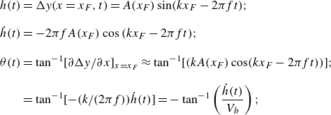 \begin{equation} \begin{aligned} h(t) &= \Delta y (x=x_F,t) = A(x_F) \sin (kx_F - 2 \pi ft ); \\[8pt] \dot {h}(t) &= -2\pi f A(x_F)\cos {(kx_F-2\pi ft )}; \\[8pt] \theta (t) &= \tan ^{-1} [ {\partial \Delta y/ \partial x} ]_{x=x_F} \approx \tan ^{-1} [ (kA(x_F)\cos (kx_F-2\pi ft))]; \\[8pt] &= \tan ^{-1} [ -(k/({2 \pi f})) \dot {h}(t) ] = -\tan ^{-1} \left ( \frac {\dot {h}(t)}{V_b} \right ); \end{aligned} \end{equation}
where $V_b= 2 \pi f/k$
is the wave velocity of the body undulation. The above expression for
$V_b= 2 \pi f/k$
is the wave velocity of the body undulation. The above expression for $\theta$
assumes that
$\theta$
assumes that $dA/dx$
is small. In the LEV-based model, the Kutta–Joukowski theorem is applied to express the force normal to the caudal fin as
$dA/dx$
is small. In the LEV-based model, the Kutta–Joukowski theorem is applied to express the force normal to the caudal fin as
 \begin{equation} F_N = \rho V \Gamma , \end{equation}
where $\Gamma$
represents the net circulation generated by the caudal fin, and
$\Gamma$
represents the net circulation generated by the caudal fin, and $V$
is the net relative velocity of the fin to the flow, defined as
$V$
is the net relative velocity of the fin to the flow, defined as $V = \sqrt {U^2 + \dot {h}^2}$
, where
$V = \sqrt {U^2 + \dot {h}^2}$
, where $U$
is the swimming speed in the surge direction. According to our findings from the force partitioning method analysis (Seo & Mittal Reference Seo and Mittal2022; Raut et al. Reference Raut, Seo and Mittal2024), the circulation
$U$
is the swimming speed in the surge direction. According to our findings from the force partitioning method analysis (Seo & Mittal Reference Seo and Mittal2022; Raut et al. Reference Raut, Seo and Mittal2024), the circulation $\Gamma$
for these flapping foils/fins is primarily due to the LEV, whose strength is proportional to the velocity component of
$\Gamma$
for these flapping foils/fins is primarily due to the LEV, whose strength is proportional to the velocity component of $V$
perpendicular to the chord of the fin. The magnitude of this velocity component is related to the instantaneous effective angle of attack (
$V$
perpendicular to the chord of the fin. The magnitude of this velocity component is related to the instantaneous effective angle of attack ( $\alpha _{\textit{eff}}$
) on the caudal fin. Thus, we assume a proportional relationship between
$\alpha _{\textit{eff}}$
) on the caudal fin. Thus, we assume a proportional relationship between $\Gamma$
and
$\Gamma$
and $\alpha _{\textit{eff}}$
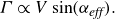 \begin{equation} \Gamma \propto V \sin (\alpha _{\textit{eff}}). \end{equation}
The instantaneous effective angle of attack, $\alpha _{\textit{eff}}$
, is calculated as
$\alpha _{\textit{eff}}$
, is calculated as
 \begin{equation} \alpha _{\textit{eff}}(t) = -\tan ^{-1}\left (\frac {\dot {h}(t)}{U}\right ) - \theta (t)= -\tan ^{-1}\left (\frac {\dot {h}(t)}{U}\right ) + \tan ^{-1} \left ( \frac {\dot {h}(t)}{V_b} \right ). \end{equation}
Given that the LEV-induced force is primarily determined by the relative flow velocity at the leading edge, $V$
, we can express the force coefficient in the normal direction,
$V$
, we can express the force coefficient in the normal direction, $C_N$
, as
$C_N$
, as
 \begin{equation} C_N = \frac {F_N}{\frac {1}{2} \rho V_{\textit{max}}^2 c}, \end{equation}
where $c$
is the length of the caudal fin and
$c$
is the length of the caudal fin and $V_{\textit{max}}$
is the maximum value of
$V_{\textit{max}}$
is the maximum value of $V$
during the tail-beat cycle. Using (2.4), we find that
$V$
during the tail-beat cycle. Using (2.4), we find that $C_N \propto \sin (\alpha _{\textit{eff}})$
. Consequently, the thrust coefficient,
$C_N \propto \sin (\alpha _{\textit{eff}})$
. Consequently, the thrust coefficient, $C_T$
, can be expressed as
$C_T$
, can be expressed as
 \begin{equation} C_T \propto \sin (\alpha _{\textit{eff}}) \sin (\theta ). \end{equation}
We define the LEV thrust factor, $\Lambda _T$
as the mean value of the right-hand side of the above expression as follows:
$\Lambda _T$
as the mean value of the right-hand side of the above expression as follows:
 \begin{equation} \Lambda _T = \langle \sin (\alpha _{\textit{eff}}) \sin (\theta ) \rangle , \end{equation}
where $\langle \cdot \rangle$
represents the mean, and based on the above expression, the mean thrust coefficient
$\langle \cdot \rangle$
represents the mean, and based on the above expression, the mean thrust coefficient $C_T$
is expected to be linearly proportional to
$C_T$
is expected to be linearly proportional to $\Lambda _T$
. Thus, using this model, the thrust can be related to the kinematics of the foil/fin via
$\Lambda _T$
. Thus, using this model, the thrust can be related to the kinematics of the foil/fin via $\Lambda _T$
. This linear relationship has been extensively verified for a pitching and heaving foil in a previous study (Raut et al. Reference Raut, Seo and Mittal2024) where we conducted 462 distinct simulations of flapping foils with different Strouhal numbers, pitch amplitudes and locations of the pitch axis. The linear correlation over this entire range was found to match with an
$\Lambda _T$
. This linear relationship has been extensively verified for a pitching and heaving foil in a previous study (Raut et al. Reference Raut, Seo and Mittal2024) where we conducted 462 distinct simulations of flapping foils with different Strouhal numbers, pitch amplitudes and locations of the pitch axis. The linear correlation over this entire range was found to match with an $R^2$
value of 0.91, which affirmed the predictive power of the model. We employ this same model in the current study but provide additional validation of the model for the caudal fins of the BCF carangiform swimmers in a later section.
$R^2$
value of 0.91, which affirmed the predictive power of the model. We employ this same model in the current study but provide additional validation of the model for the caudal fins of the BCF carangiform swimmers in a later section.
2.2. Modelling thrust enhancement due to hydrodynamic interactions in a fish school
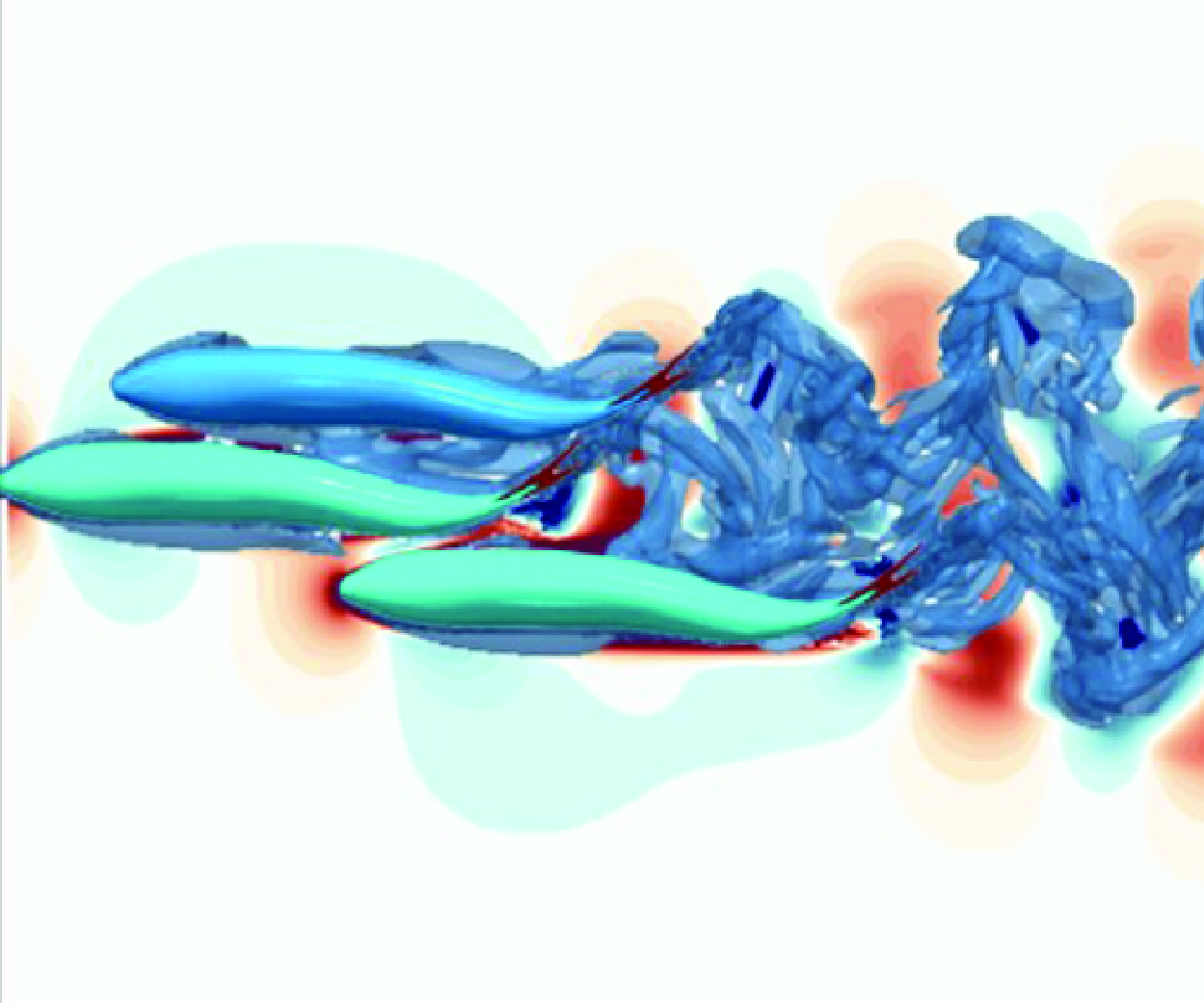
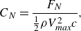
The primary hydrodynamic distinction between swimming alone and within a school for a fish is the ability to exploit the wake produced by other swimmers to improve its swimming performance. One significant characteristic of this wake field is the perturbation in velocity, with the lateral component being particularly dominant (Seo & Mittal Reference Seo and Mittal2022). This lateral velocity perturbation alters the relative velocity normal to the caudal fin of a trailing fish, as depicted in figure 2. When the local velocity perturbation $(u'v')$
are included, the effective angle of attack between the incident flow and the caudal fin changes from
$(u'v')$
are included, the effective angle of attack between the incident flow and the caudal fin changes from $\alpha _{\textit{eff}}$
to
$\alpha _{\textit{eff}}$
to $\alpha ^\prime _{\textit{eff}}$
 \begin{equation} \alpha _{\textit{eff}}^{\prime }(t) = \tan ^{-1}\left (\frac {-\dot {h}(t)+v^{\prime }(t)}{U+u^{\prime }(t)}\right ) - \theta (t); \quad \Lambda ^{\prime }_T = \langle \sin (\alpha ^{\prime }_{\textit{eff}}) \sin (\theta ) \rangle . \end{equation}
Illustration of the LEV-based model used in this study. (a) Vortex structure of a minimal school of two fish swimming in tandem, with the trailing fish positioned to interact with the wake produced by the leading fish. (b) Schematic representation showing the relative positioning of the leading and trailing fish, highlighting the motion of the caudal fin ( $\dot {h}$
) and flow perturbations
$\dot {h}$
) and flow perturbations $(u', v')$
. (c) Diagram of the caudal fin of the trailing fish, illustrating the effective angle of attack,
$(u', v')$
. (c) Diagram of the caudal fin of the trailing fish, illustrating the effective angle of attack, $\alpha _{\textit{eff}}$
, and the modified angle,
$\alpha _{\textit{eff}}$
, and the modified angle, $\alpha '_{\textit{eff}}$
, due to flow perturbations. The diagram highlights the influence of relative velocity components
$\alpha '_{\textit{eff}}$
, due to flow perturbations. The diagram highlights the influence of relative velocity components $(U + u')$
and
$(U + u')$
and $(-\dot {h} + v')$
on thrust generation.
$(-\dot {h} + v')$
on thrust generation.
This change affects the strength of the LEV generated on the caudal fin of the trailing fish, and if the movement of the caudal fin is timed appropriately with respect to this velocity perturbation, it can augment the thrust force for the trailing fish. Per this LEVBM, any improvement in thrust is proportional to
 \begin{equation} \varDelta \Lambda _T = \Lambda ^{\prime }_T - \Lambda _T, \end{equation}
and we use this parameter (specifically, the relative increase relative to the baseline value, i.e. $(\varDelta \Lambda _T/\Lambda _T) \times 100 \, \%$
) for quantifying the effect of hydrodynamic interactions on the thrust of trailing fish. Note that, based on this expression, the change in thrust for a trailing fish whose caudal fin is located at
$(\varDelta \Lambda _T/\Lambda _T) \times 100 \, \%$
) for quantifying the effect of hydrodynamic interactions on the thrust of trailing fish. Note that, based on this expression, the change in thrust for a trailing fish whose caudal fin is located at $ ( X_T,Y_T )$
relative to the caudal fin of the leading fish, is a function of the wake perturbation to the velocity at that location due to the leading fish, i.e.
$ ( X_T,Y_T )$
relative to the caudal fin of the leading fish, is a function of the wake perturbation to the velocity at that location due to the leading fish, i.e. $(u^\prime , v^\prime ) = ( u_L(X_T,t)-U, v_L(X_T,t) )$
, where
$(u^\prime , v^\prime ) = ( u_L(X_T,t)-U, v_L(X_T,t) )$
, where $ ( u_L(X_T,t), v_L(X_T,t) )$
represents the velocity field in the wake of leading fish. The fin kinematics of the trailing fish can be expressed via
$ ( u_L(X_T,t), v_L(X_T,t) )$
represents the velocity field in the wake of leading fish. The fin kinematics of the trailing fish can be expressed via $ ( h_T(t), \theta _T(t), \phi _T )$
. Thus, the thrust change for a trailing fish at any location for a given wake of a leading fish can be expressed in a functional form as
$ ( h_T(t), \theta _T(t), \phi _T )$
. Thus, the thrust change for a trailing fish at any location for a given wake of a leading fish can be expressed in a functional form as
 \begin{equation} \varDelta \Lambda _T= \varDelta \Lambda _T \left [ u_L(X_T,t), v_L(X_T,t), h_T(t), \theta _T(t), \phi _T \right ]. \end{equation}
It should be noted that since the velocity perturbation in the wake of the leading fish is a function of the kinematic parameters of the leading fish, the above functional relationship can also be expressed as
 \begin{equation} \varDelta \Lambda _T= \varDelta \Lambda _T \left [ h_L(t), \theta _L(t), \phi _L; X_T, Y_T, h_T(t), \theta _T(t), \phi _T \right ], \end{equation}
where the first three parameters depend on the leading fish and the last five parameters on the trailing fish. ‘Thrust enhancement maps’ of this quantity $\varDelta \Lambda _T$
will be used to interpret the results of this study.
$\varDelta \Lambda _T$
will be used to interpret the results of this study.
There are several assumptions regarding the hydrodynamics in the above model for thrust prediction of the trailing fish. Among these is the assumption that the body of the trailing fish does not affect the velocity perturbation experienced by the caudal fin. The relatively large body combined with its upstream placement relative to the caudal fin makes this an important assumption. Other notable assumptions are that the movement of the caudal fin of the trailing fish does not affect the $ ( u^\prime , v^\prime )$
experienced by the fin – i.e. we neglect ‘self-induction’ effects of the trailing fish’s caudal fin on flow immediately upstream of itself. Finally, the LEVBM also does not account for the specific three-dimensional shape of the caudal fin. We will examine these assumptions later in the paper.
$ ( u^\prime , v^\prime )$
experienced by the fin – i.e. we neglect ‘self-induction’ effects of the trailing fish’s caudal fin on flow immediately upstream of itself. Finally, the LEVBM also does not account for the specific three-dimensional shape of the caudal fin. We will examine these assumptions later in the paper.
3. Results
3.1. Direct numerical simulation of a BCF carangiform swimmer
To resolve the flow field around the swimming fish, we use a sharp-interface, immersed boundary solver, ViCar3D (Mittal et al. Reference Mittal, Dong, Bozkurttas, Najjar, Vargas and von Loebbecke2008), to solve the incompressible Navier–Stokes equations with second-order finite difference in time and space. This solver has been validated extensively in previous studies of bio-locomotion flows (Seo & Mittal Reference Seo and Mittal2022; Zhou et al. Reference Zhou, Seo and Mittal2023; Zhou et al. Reference Zhou, Seo and Mittal2024; Kumar, Seo & Mittal Reference Kumar, Seo and Mittal2025; Mittal et al. Reference Mittal, Seo, Turner, Kumar, Prakhar and Zhou2025).
The solitary fish is tethered to a fixed location in an incoming flow in these simulations. Through trial and error, the incoming flow velocity is set to a value of $0.48fL$
for which, the total mean surge force on the fish is nearly zero. This models the condition where the fish is swimming at its terminal velocity. The same inflow velocity is then imposed on all the fish when the various fish school configurations are simulated. The final swimming condition corresponds to a length-based Reynolds number of
$0.48fL$
for which, the total mean surge force on the fish is nearly zero. This models the condition where the fish is swimming at its terminal velocity. The same inflow velocity is then imposed on all the fish when the various fish school configurations are simulated. The final swimming condition corresponds to a length-based Reynolds number of $\boldsymbol{\boldsymbol{Re}}=UL/\nu =5000$
. The Strouhal number based on the swimming velocity and the peak-to-peak amplitude of the caudal fin trailing edge is
$\boldsymbol{\boldsymbol{Re}}=UL/\nu =5000$
. The Strouhal number based on the swimming velocity and the peak-to-peak amplitude of the caudal fin trailing edge is $2A(x_F)f/U=0.42$
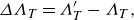
. Figure 3(b) shows the instantaneous vortex structure of the solitary swimming fish. The tailbeat motion generates two sets of vortex loops, propagating downstream at an oblique angle to the wake centreline. The streamwise forces on the fish body are decomposed into pressure and viscous stress forces on the body and the caudal fin and plotted in figure 3(c). The viscous shear drag on the body of the fish is the main source of drag, while the pressure force from the caudal fin dominates the generation of thrust, contributing to about
$2A(x_F)f/U=0.42$
. Figure 3(b) shows the instantaneous vortex structure of the solitary swimming fish. The tailbeat motion generates two sets of vortex loops, propagating downstream at an oblique angle to the wake centreline. The streamwise forces on the fish body are decomposed into pressure and viscous stress forces on the body and the caudal fin and plotted in figure 3(c). The viscous shear drag on the body of the fish is the main source of drag, while the pressure force from the caudal fin dominates the generation of thrust, contributing to about $96\, \%$
of the total thrust force.
$96\, \%$
of the total thrust force.
Simulation of a solitary BCF swimmer. (a) Computational domain for solitary fish swimming, with spatial dimensions shown in terms of normalised body length, $L$
. The flow direction is from
$L$
. The flow direction is from $-x$
to
$-x$
to $+x$
. (b) Instantaneous three-dimensional vortex structure of the fish, visualised by the iso-surface of
$+x$
. (b) Instantaneous three-dimensional vortex structure of the fish, visualised by the iso-surface of $Q/f^2 = 1$
, coloured by the lateral velocity,
$Q/f^2 = 1$
, coloured by the lateral velocity, $v/U$
. (c) Pressure and viscous shear forces on the fish body and caudal fin in the streamwise direction. Forces are normalised as
$v/U$
. (c) Pressure and viscous shear forces on the fish body and caudal fin in the streamwise direction. Forces are normalised as $F^*=F/(\rho L^4f^2)$
, and
$F^*=F/(\rho L^4f^2)$
, and $T=1/f$
is the period of tailbeat.
$T=1/f$
is the period of tailbeat.
3.2. Thrust enhancement map for a two-fish configuration
3.2.1. Generation of thrust enhancement maps
We start by examining the thrust enhancement map for a two-fish configuration where both fish have exactly the same swimming kinematics in terms of frequency, amplitude and phase. We summarise the process used to predict these hydrodynamic interactions in fish (see figure 4). Once the wake velocity field (i.e. $ (u_L (x,y,t), v_L (x,y,t) )$
) for the leading fish is obtained via a direct numerical simulation, a trailing fish is virtually placed in this wake field at a location with its caudal fin located at
$ (u_L (x,y,t), v_L (x,y,t) )$
) for the leading fish is obtained via a direct numerical simulation, a trailing fish is virtually placed in this wake field at a location with its caudal fin located at $ ( X_T,Y_T )$
relative to the caudal fin of the leading fish on the centre plane of the leading fish. The wake velocity at
$ ( X_T,Y_T )$
relative to the caudal fin of the leading fish on the centre plane of the leading fish. The wake velocity at $ ( X_T,Y_T )$
is then combined with the kinematics of the caudal fin of the virtual trailing fish to estimate the interaction effect on the thrust enhancement factor
$ ( X_T,Y_T )$
is then combined with the kinematics of the caudal fin of the virtual trailing fish to estimate the interaction effect on the thrust enhancement factor $\varDelta \Lambda _T$
via the expression in (2.7)
$\varDelta \Lambda _T$
via the expression in (2.7) $-$
(2.12). Based on the linear relationship between
$-$
(2.12). Based on the linear relationship between $\Lambda _T$
and
$\Lambda _T$
and $C_T$
(see (2.7)), the
$C_T$
(see (2.7)), the $\varDelta \Lambda _T$
is used as a surrogate for the change in thrust of the trailing fish. A thrust enhancement map is then generated by placing the virtual trailing fish at various locations within the domain with minimal computational expense.
$\varDelta \Lambda _T$
is used as a surrogate for the change in thrust of the trailing fish. A thrust enhancement map is then generated by placing the virtual trailing fish at various locations within the domain with minimal computational expense.
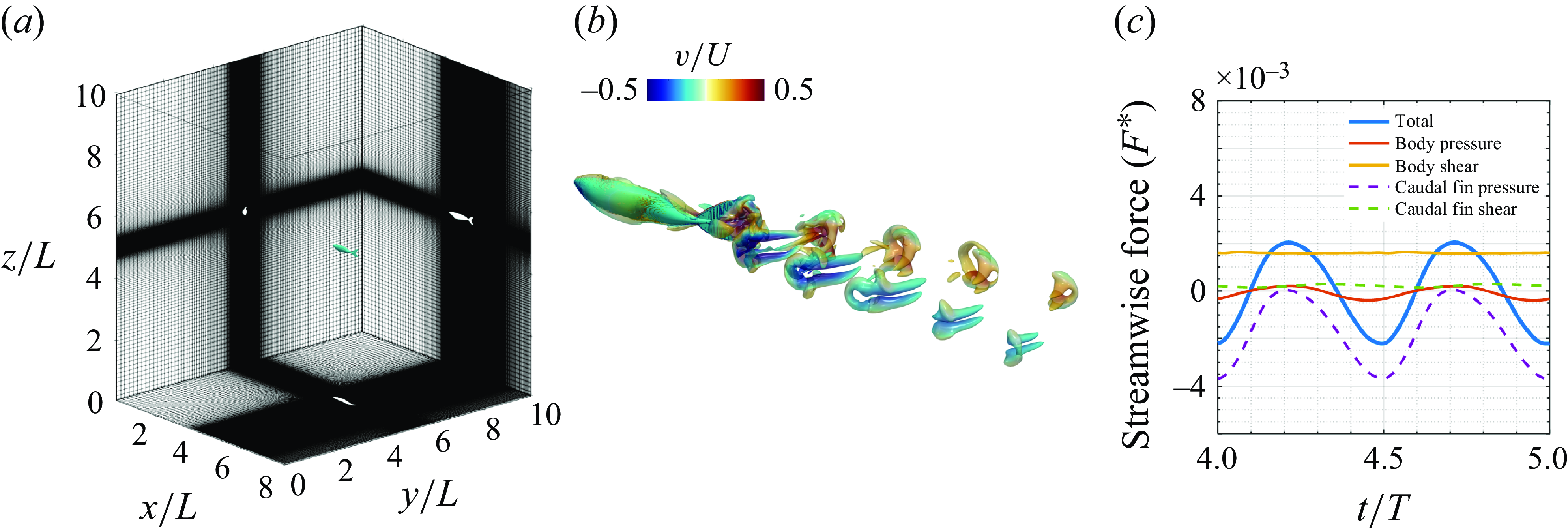
The LEVBM-based thrust enhancement map for a two-fish configuration. Instantaneous (a) streamwise $(u'/U)$
and (b) lateral
$(u'/U)$
and (b) lateral $(v'/U)$
velocity components of a solitary swimmer. Velocity components are extracted from the centre plane during one tailbeat cycle. (c) The
$(v'/U)$
velocity components of a solitary swimmer. Velocity components are extracted from the centre plane during one tailbeat cycle. (c) The $\varDelta \Lambda _T$
map (
$\varDelta \Lambda _T$
map ( $\varDelta \phi = 0$
,
$\varDelta \phi = 0$
, $A = 1$
and
$A = 1$
and $f = 1$
) with invalid regions masked, illustrating the prediction of the thrust generation of the trailing fish. (d) Zoomed-in
$f = 1$
) with invalid regions masked, illustrating the prediction of the thrust generation of the trailing fish. (d) Zoomed-in $\varDelta \Lambda _T$
map of (c), showing beneficial (red) and detrimental (blue) regions for a trailing fish. The region at the left of the green line is invalid if the trailing fish is the same size as the leading fish.
$\varDelta \Lambda _T$
map of (c), showing beneficial (red) and detrimental (blue) regions for a trailing fish. The region at the left of the green line is invalid if the trailing fish is the same size as the leading fish.
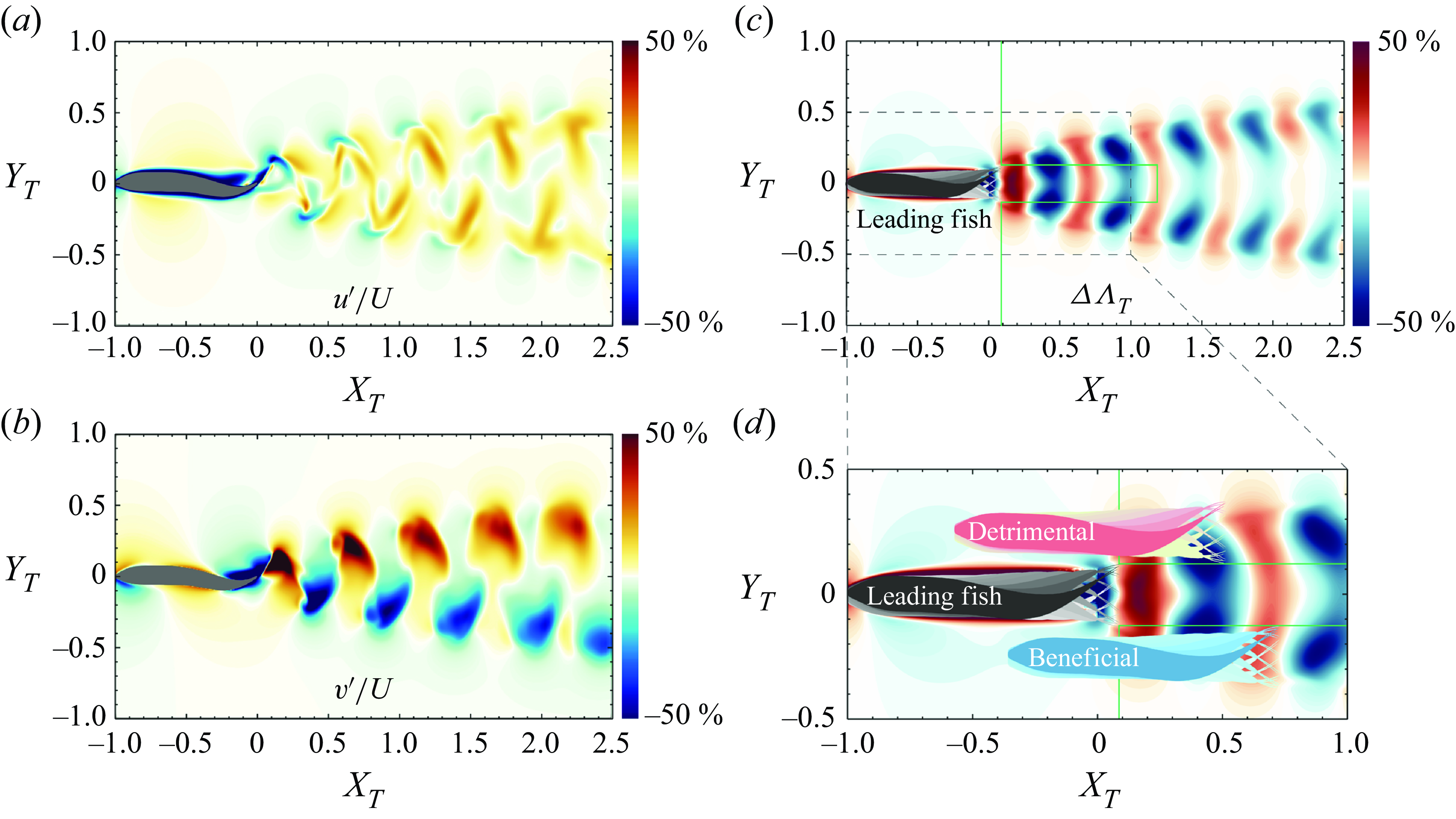
Figure 4(c) shows the thrust enhancement map generated based on the above procedure. We highlight a small rectangular region behind the leading fish where the trailing fish cannot be placed since this would lead to collisions between two fish. We also exclude positions of the trailing fish that would place it ahead of the leading fish. Figure 4(d) shows two notional positions of a trailing fish on the thrust enhancement map that would correspond to either a beneficial or a detrimental interaction. In figure 4(d), the blue trailing fish is positioned with its caudal fin within the positive $\varDelta \Lambda _T$
region and would benefit from a constructive interaction with the leading fish’s wake, generating more thrust than a solitary swimmer. In contrast, the pink trailing fish, with its caudal fin located in a negative
$\varDelta \Lambda _T$
region and would benefit from a constructive interaction with the leading fish’s wake, generating more thrust than a solitary swimmer. In contrast, the pink trailing fish, with its caudal fin located in a negative $\varDelta \Lambda _T$
region, would experience a reduction in thrust.
$\varDelta \Lambda _T$
region, would experience a reduction in thrust.
3.2.2. Verification of thrust enhancement maps
As pointed out earlier, several assumptions are inherent in the prediction of thrust for the trailing fish based on the LEVBM, and we have carried out comprehensive verifications of the model predictions to assess these assumptions.
As noted above, a known limitation of the LEVBM is that it does not account for the effect of the body of the trailing fish on the wake perturbations encountered by the caudal fin of the trailing fish. Other key assumptions are neglecting the effect of the trailing fish’s caudal fin on the encountered wake perturbation and the inability to account for the effect of the three-dimensional shape of the caudal fin of the trailing fish on thrust enhancement. The LEVBM also neglects intrinsically unsteady effects of the leading fish wake on the thrust of the trailing fish – these include for instance the added-mass effects associated with heaving as well as effects associated with angular acceleration of leading edge. However, the effect of the presence of the body of the trailing fish is expected to be the most important. Thus, in the first set of direct numerical simulations (DNS), we exclude the body of the trailing fish (see figure 5(a) for the configuration) to test the effect of the latter two assumptions on the LEVBM predictions.
Direct numerical simulations of two-fish schools. Top and isometric views of the instantaneous three-dimensional vortex structures of two-fish schools. Trailing fish with ((a) fin only, and with (b) body + fin). Vortex structures are visualised using iso-surfaces of $Q = 1f^2$
and coloured by the normalised lateral velocity
$Q = 1f^2$
and coloured by the normalised lateral velocity $(v/U)$
, where
$(v/U)$
, where $U$
is the steady swimming speed of the fish.
$U$
is the steady swimming speed of the fish.
For 14 selected locations of the trailing fish, which cover a range of placements with beneficial and detrimental interactions (as noted in figure 6
a), we compare the thrust enhancement predictions from the LEVBM directly with the thrust enhancement of the pressure component on the fin calculated from the DNS. Figure 6(c) shows the correlation between the predicted $\varDelta \Lambda _T$
values and the thrust change (
$\varDelta \Lambda _T$
values and the thrust change ( $\Delta T$
) obtained from the DNS results corresponding to the case where the body of the trailing fish is excluded. A best-fit line between the two data sets suggests a linear relationship with a high degree of correlation (
$\Delta T$
) obtained from the DNS results corresponding to the case where the body of the trailing fish is excluded. A best-fit line between the two data sets suggests a linear relationship with a high degree of correlation ( $R^2 = 0.9$
). The equation of the best-fit line has a slope of 0.91 with zero intercept corresponding to 0.06 %, which signifies an excellent one-to-one relationship between the LEVBM prediction and the DNS. All in all, the above comparison suggests that the latter two assumptions discussed in the previous paragraph do not significantly deteriorate the predictions of the LEVBM, and it performs quite well despite the complex shape and effect of the caudal fin.
$R^2 = 0.9$
). The equation of the best-fit line has a slope of 0.91 with zero intercept corresponding to 0.06 %, which signifies an excellent one-to-one relationship between the LEVBM prediction and the DNS. All in all, the above comparison suggests that the latter two assumptions discussed in the previous paragraph do not significantly deteriorate the predictions of the LEVBM, and it performs quite well despite the complex shape and effect of the caudal fin.
Verification of the $\varDelta \Lambda _T$
map using direct numerical simulations. (a) Zoomed-in view of a subdomain of the
$\varDelta \Lambda _T$
map using direct numerical simulations. (a) Zoomed-in view of a subdomain of the $\varDelta \Lambda _T$
contour map for two-fish schooling, indicating beneficial and detrimental interaction regions. Highlighted dots show the locations of the tail of the trailing fish from positions
$\varDelta \Lambda _T$
contour map for two-fish schooling, indicating beneficial and detrimental interaction regions. Highlighted dots show the locations of the tail of the trailing fish from positions $a$
to
$a$
to $n$
$n$ $(N = 14)$
. The region at the left of the green line is invalid if the trailing fish is the same size as the leading fish. (b) Instantaneous three-dimensional vortex structures of two-fish schools corresponding to
$(N = 14)$
. The region at the left of the green line is invalid if the trailing fish is the same size as the leading fish. (b) Instantaneous three-dimensional vortex structures of two-fish schools corresponding to $a$
,
$a$
, $d$
and
$d$
and $m$
in (a). (c,d) Linear correlation between
$m$
in (a). (c,d) Linear correlation between $\varDelta \Lambda _T$
(%) from the LEVBM and
$\varDelta \Lambda _T$
(%) from the LEVBM and $\Delta T$
(%) (i.e. thrust change) from DNS, with (c) for fin only with an
$\Delta T$
(%) (i.e. thrust change) from DNS, with (c) for fin only with an $R^2$
value of 0.9 and a corresponding best-fit line of
$R^2$
value of 0.9 and a corresponding best-fit line of $\Delta T\, \%=0.91\varDelta \Lambda _T\, \%+0.060\, \%$
) (d) for body+fin with an
$\Delta T\, \%=0.91\varDelta \Lambda _T\, \%+0.060\, \%$
) (d) for body+fin with an $R^2$
value of 0.7 and a corresponding best-fit line corresponding to
$R^2$
value of 0.7 and a corresponding best-fit line corresponding to $\Delta T\, \%=0.29\varDelta \Lambda _T\, \%+3.7\, \%$
).
$\Delta T\, \%=0.29\varDelta \Lambda _T\, \%+3.7\, \%$
).
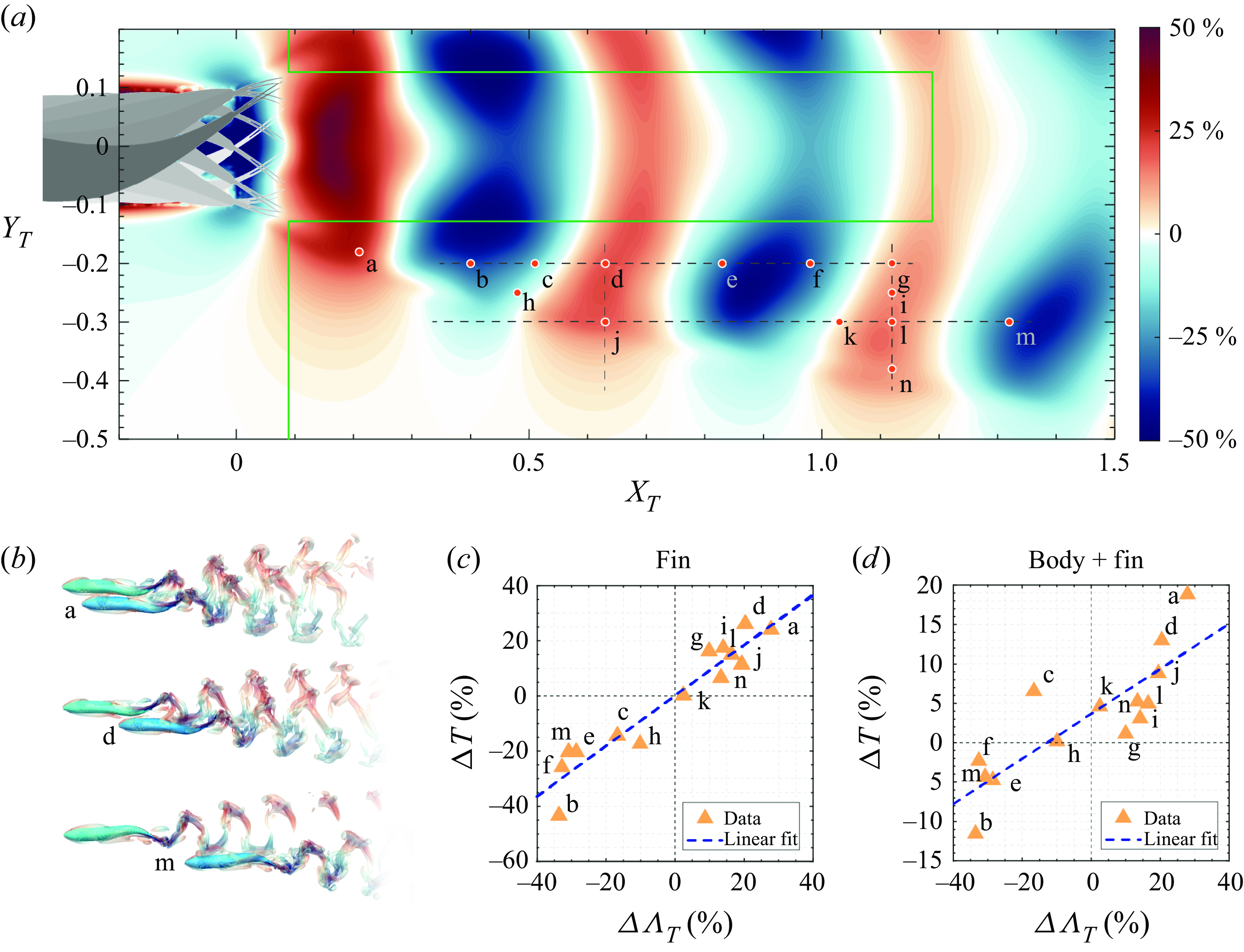
In the second and final stage of verification, we reintroduce the body of the trailing fish into the DNS to examine the effect of the body on the LEVBM thrust enhancement map predictions, and figure 6(d) shows the correlation between the DNS estimation of the pressure thrust on the fin and the LEVBM predictions. With the body of the trailing fish included, the linear correlation reduces to a $R^2$
of 0.7, which suggests that, while the presence of the fish body does diminish the predictive power of the LEVBM, the linear correlation remains acceptable, and the model is still useful for predicting the thrust changes for fish schools. This verification also confirms that other assumptions such as the exclusion of intrinsically unsteady effects also do have a significant deleterious effect on model predictions.
$R^2$
of 0.7, which suggests that, while the presence of the fish body does diminish the predictive power of the LEVBM, the linear correlation remains acceptable, and the model is still useful for predicting the thrust changes for fish schools. This verification also confirms that other assumptions such as the exclusion of intrinsically unsteady effects also do have a significant deleterious effect on model predictions.
We also note that the slope and intercept of the best-fit line are 0.29 % and 3.7 %, respectively. This significant reduction in slope from the expected value of unity indicates that for the fish model in the current study, the body acts to diminish the effect of the hydrodynamic interactions on the thrust of the caudal fin. This is likely due to the fact that the most significant effect on the effective angle of attack of the trailing caudal fin is via the perturbation in the lateral velocity, and the body acts as a ‘wall’ and diminishes these lateral perturbations of vortex structure that convects past it to the fin. However, this body effect might depend on the precise shape of the body, the fin and the kinematics of the body. For fins such as those of sharks that are highly extended in the dorso-ventral directions, much of the fin is located significantly far from the influence of the body and may be less affected by the body effect. In contrast, a fish such as tuna has a very thick body with a fin that is more influenced by the flow effects generated by the body. The length of the fish might also matter since this will change the time taken for the flow to travel from the nose of the fish to the fin, thereby changing the phasing of the body induced flow and the fin motion. Finally, we have not incorporated the effect of other fins (midline and paired fins) in this study. All of these effects open up a vast parameter space but would be interesting issues to explore in a future study.
3.2.3. Observations regarding the topology of the thrust enhancement maps
The periodic distribution of positive and negative regions of the $\varDelta \Lambda _T$
in the streamwise direction is a result of the alternating shedding of vortices from the leading fish’s tail, which convects downstream with the flow and drives the velocity perturbation pattern in the wake. As shown by Seo & Mittal (Reference Seo and Mittal2022), the thrust enhancement is associated with the effective phase difference between the tail beats of the leading and trailing fish
$\varDelta \Lambda _T$
in the streamwise direction is a result of the alternating shedding of vortices from the leading fish’s tail, which convects downstream with the flow and drives the velocity perturbation pattern in the wake. As shown by Seo & Mittal (Reference Seo and Mittal2022), the thrust enhancement is associated with the effective phase difference between the tail beats of the leading and trailing fish $\varDelta \phi _{\textit{eff}}$
, which is estimated by the following expression:
$\varDelta \phi _{\textit{eff}}$
, which is estimated by the following expression:
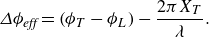 \begin{equation} \varDelta \phi _{\textit{eff}} = \left ( \phi _T- \phi _L \right ) - \frac {2\pi X_T}{\lambda }. \end{equation}
Here, $\phi _T$
and
$\phi _T$
and $\phi _L$
are the tailbeat phases of the trailing and leading fish, respectively, and
$\phi _L$
are the tailbeat phases of the trailing and leading fish, respectively, and $\lambda$
represents the wavelength of the velocity perturbation in the wake, which may be estimated as
$\lambda$
represents the wavelength of the velocity perturbation in the wake, which may be estimated as $\lambda \approx U/f_L$
, where
$\lambda \approx U/f_L$
, where $U$
is the swimming speed and
$U$
is the swimming speed and $f_L$
is the tailbeat frequency of the leading fish. The effective phase difference is directly related to the phase difference between
$f_L$
is the tailbeat frequency of the leading fish. The effective phase difference is directly related to the phase difference between $-\dot {h}_T(t)$
and
$-\dot {h}_T(t)$
and $v_L^{\prime }(X_T,t)$
in (2.9), and it determines the changes in
$v_L^{\prime }(X_T,t)$
in (2.9), and it determines the changes in $\alpha _{\textit{eff}}$
. This suggests that the phase difference between the tail beats of the two fish, as well as the trailing fish location
$\alpha _{\textit{eff}}$
. This suggests that the phase difference between the tail beats of the two fish, as well as the trailing fish location $X_T$
and the tail-beat frequency
$X_T$
and the tail-beat frequency $f_L$
of the leading fish are all factors that affect the thrust enhancement map.
$f_L$
of the leading fish are all factors that affect the thrust enhancement map.
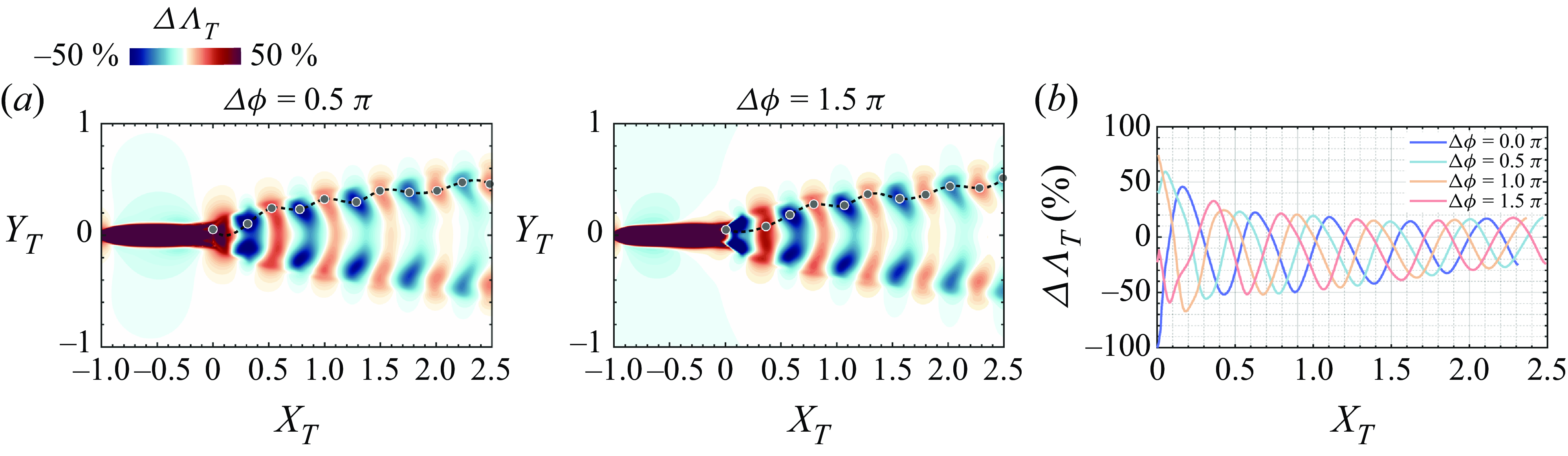
The above expression also suggests that the effects of differences in tail-beat phase $\varDelta \phi = ( \phi _T- \phi _L )$
and separation
$\varDelta \phi = ( \phi _T- \phi _L )$
and separation $X_T$
between the two fish are essentially interchangeable in the near wake. In figure 7(a), thrust enhancement maps for two additional
$X_T$
between the two fish are essentially interchangeable in the near wake. In figure 7(a), thrust enhancement maps for two additional $\varDelta \phi$
are shown alongside the
$\varDelta \phi$
are shown alongside the $\varDelta \Lambda _T$
plots along the locus of the extreme values of these quantities for four different choices of
$\varDelta \Lambda _T$
plots along the locus of the extreme values of these quantities for four different choices of $\varDelta \phi$
. We note that the topology of the thrust enhancement maps for the different phases is very similar except for a shift in the streamwise direction. This is confirmed by the peak locus plot in figure 7(b), which shows that all the different cases of
$\varDelta \phi$
. We note that the topology of the thrust enhancement maps for the different phases is very similar except for a shift in the streamwise direction. This is confirmed by the peak locus plot in figure 7(b), which shows that all the different cases of $\varDelta \phi$
are essentially the same except for this shift. This suggests that a trailing swimmer can improve thrust at any given streamwise location by suitably adjusting its flapping phase. Similarly, for a given phase difference, the trailing swimmer can gain thrust benefit by moving to an appropriate location in the wake.
$\varDelta \phi$
are essentially the same except for this shift. This suggests that a trailing swimmer can improve thrust at any given streamwise location by suitably adjusting its flapping phase. Similarly, for a given phase difference, the trailing swimmer can gain thrust benefit by moving to an appropriate location in the wake.
The $\varDelta \Lambda _T$
maps for two-fish schooling at different tailbeat phases. (a) The
$\varDelta \Lambda _T$
maps for two-fish schooling at different tailbeat phases. (a) The $\varDelta \Lambda _T$
maps for two different phase differences
$\varDelta \Lambda _T$
maps for two different phase differences $(\varDelta \phi )$
between the leading and trailing fish. (b) Presents
$(\varDelta \phi )$
between the leading and trailing fish. (b) Presents $\varDelta \Lambda _T$
values along curves connecting peaks and valleys on contours of corresponding
$\varDelta \Lambda _T$
values along curves connecting peaks and valleys on contours of corresponding $\varDelta \Lambda _T$
maps, demonstrated as grey dots and dashed lines in (a). These profiles highlight variations in
$\varDelta \Lambda _T$
maps, demonstrated as grey dots and dashed lines in (a). These profiles highlight variations in $\varDelta \Lambda _T$
along the streamwise direction
$\varDelta \Lambda _T$
along the streamwise direction $(X_T)$
, illustrating how phase influences the thrust enhancement of the trailing fish.
$(X_T)$
, illustrating how phase influences the thrust enhancement of the trailing fish.
Several other features of the thrust enhancement map are worth noting for their implication for schooling. First, there are multiple regions where the thrust is enhanced in the wake, but these regions are interspersed with regions where the thrust is reduced due to the hydrodynamic interactions. The extreme values of thrust change are located along two oblique angles from the centre of the wake that correspond well to the double-vortex loop wake that is generated behind the flapping fin. The region near the wake centre has relatively low values of $\varDelta \Lambda _T$
.
$\varDelta \Lambda _T$
.
Figure 7(b) shows the value of $\varDelta \Lambda _T$
along the local peaks in this parameter and this pattern also decays relatively slowly in the wake. Indeed, while the peak in
$\varDelta \Lambda _T$
along the local peaks in this parameter and this pattern also decays relatively slowly in the wake. Indeed, while the peak in $\varDelta \Lambda _T$
around
$\varDelta \Lambda _T$
around $X_T \sim 0.5$
corresponds to a 25 % increase in
$X_T \sim 0.5$
corresponds to a 25 % increase in $\varDelta \Lambda _T$
, the peak at a distance of 2.5 body lengths is still 20 %. Thus, even in a minimal two-fish school, the trailing fish could achieve comparable propulsion benefits in many different locations within the wake of a leading fish. Second, even small changes in the movement of the leading fish would perturb the entire wake pattern and require the trailing fish to make larger adjustments in its location and/or flapping kinematics to recover to a beneficial state.
$\varDelta \Lambda _T$
, the peak at a distance of 2.5 body lengths is still 20 %. Thus, even in a minimal two-fish school, the trailing fish could achieve comparable propulsion benefits in many different locations within the wake of a leading fish. Second, even small changes in the movement of the leading fish would perturb the entire wake pattern and require the trailing fish to make larger adjustments in its location and/or flapping kinematics to recover to a beneficial state.
3.2.4. Detrimental wake interactions – analysis and implications
As noted earlier, for each region in the wake where the thrust is enhanced due to the hydrodynamic interactions, there is an adjoining region where the thrust is reduced due to these interactions. The presence of regions in the wake where the interactions are detrimental to the trailing fish is not surprising and was shown in our earlier work as well Seo & Mittal (Reference Seo and Mittal2022). However, the LEVBM thrust enhancement map shows that the detrimental effects exceed the beneficial effects, and they also extend over larger regions of the wake than the beneficial regions. This feature is unexpected and we therefore examine this in more detail. Figure 6(c), which shows the correlation between the LEVBM and the DNS for the cases where the body of the trailing fish is excluded, confirms this bias towards detrimental interactions since the negative peaks in relative thrust reach −43.3 % whereas the positive peaks are limited to + 26.1 %. Thus, the negative bias is not an erroneous prediction from the LEVBM but is confirmed by the DNS. We now examine the flow physics that results in this negative bias.
For a fish swimming in the wake of another fish, the flow perturbations due to the wake vortices, experienced by the caudal fin of the trailing fish will modify $\sin ({\alpha _{\textit{eff}}(t)})$
and through it, the thrust force. To understand this effect, we consider the velocity field in the wake of the leading fish in terms of a mean (denoted by ‘bar’) and a fluctuation (denoted by a double-prime) as follows:
$\sin ({\alpha _{\textit{eff}}(t)})$
and through it, the thrust force. To understand this effect, we consider the velocity field in the wake of the leading fish in terms of a mean (denoted by ‘bar’) and a fluctuation (denoted by a double-prime) as follows:
 \begin{equation} \left [ u_L(x,y,t) , v_L(x,y,t) \right ] = \left [ \bar {u}_L(x,y) , \bar {v}_L(x,y) \right ] + \left [ u_L^{\prime \prime } (x,y,t) , v_L^{\prime \prime }(x,y,t) \right ] . \end{equation}
We can now define an effective angle of attack due to the effect of the mean flow ( $\bar {\alpha }_{\textit{eff}}(t)$
) as follows:
$\bar {\alpha }_{\textit{eff}}(t)$
) as follows:
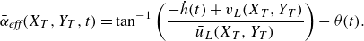 \begin{equation} \bar {\alpha }_{\textit{eff}}(X_T,Y_T,t) = \tan ^{-1}\left (\frac {-\dot {h}(t)+\bar {v}_L(X_T,Y_T)}{\bar {u}_L(X_T,Y_T)}\right ) - \theta (t). \quad \end{equation}
Similarly, the change in the thrust factor can be decomposed into
 \begin{equation} \varDelta \Lambda _T = \varDelta \bar {\Lambda }_T + \varDelta \Lambda _T^{\prime \prime } ,\end{equation}
where $\varDelta \bar {\Lambda }_T = \langle \sin {(\bar {\alpha }_{\textit{eff}})} \sin (\theta ) \rangle$
is the change in thrust factor due to the mean wake and
$\varDelta \bar {\Lambda }_T = \langle \sin {(\bar {\alpha }_{\textit{eff}})} \sin (\theta ) \rangle$
is the change in thrust factor due to the mean wake and $\varDelta \Lambda _T^{\prime \prime } = \varDelta \Lambda _T - \varDelta \bar {\Lambda }_T$
is the remaining component that is primarily associated with the velocity fluctuation in the wake. This simple decomposition now allows us to dissect the effect of the wake on the performance of the trailing fish.
$\varDelta \Lambda _T^{\prime \prime } = \varDelta \Lambda _T - \varDelta \bar {\Lambda }_T$
is the remaining component that is primarily associated with the velocity fluctuation in the wake. This simple decomposition now allows us to dissect the effect of the wake on the performance of the trailing fish.
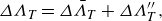
Figure 8(a) shows contour plots of $\bar {u}_L(X_T,Y_T)$
and
$\bar {u}_L(X_T,Y_T)$
and $\bar {v}_L(X_T,Y_T)$
and we note that the mean streamwise velocity in the wake symmetric about the centreline and the values are within
$\bar {v}_L(X_T,Y_T)$
and we note that the mean streamwise velocity in the wake symmetric about the centreline and the values are within $\pm 10 \, \%$
of the swimming speed. In contrast, the mean lateral velocity is anti-symmetric about the wake centreline with values up to
$\pm 10 \, \%$
of the swimming speed. In contrast, the mean lateral velocity is anti-symmetric about the wake centreline with values up to $\pm 25.6 \, \%$
of the swimming speed. The lower part of the wake has a mean lateral component that has a negative (downwards) induced velocity, and vice versa for the upper part of the wake.
$\pm 25.6 \, \%$
of the swimming speed. The lower part of the wake has a mean lateral component that has a negative (downwards) induced velocity, and vice versa for the upper part of the wake.
Contours of the time-averaged velocity components in the wake of the solitary fish swimming. (a) Contour plot of the streamwise velocity component $\bar {u}_L/U.$
(b) Contour plot of the lateral velocity component
$\bar {u}_L/U.$
(b) Contour plot of the lateral velocity component $\bar {v}_L/U.$
the red dot at
$\bar {v}_L/U.$
the red dot at $(X_T, Y_T) = (0.63,-0.2)$
represents the position d in figure 6.
$(X_T, Y_T) = (0.63,-0.2)$
represents the position d in figure 6.
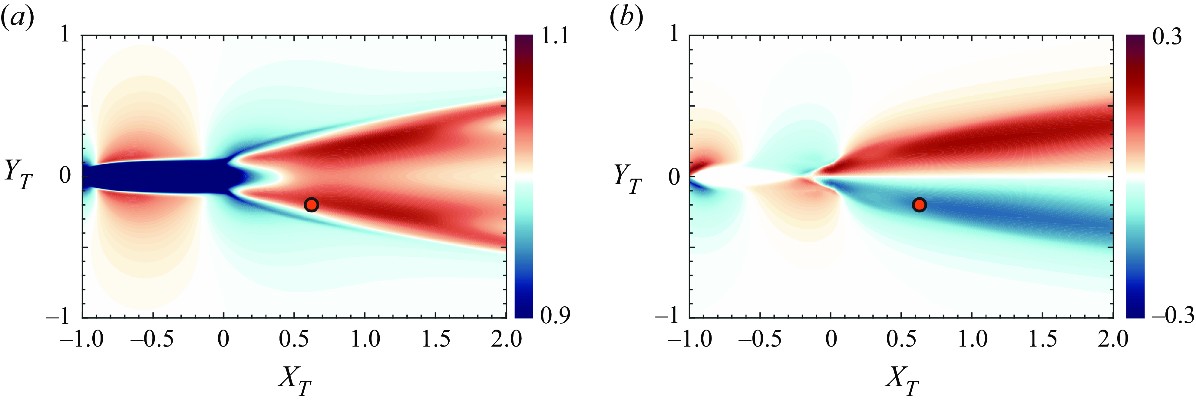
Figure 9(a) shows contours of $\varDelta \bar {\Lambda }_T$
for the case with
$\varDelta \bar {\Lambda }_T$
for the case with $\varDelta \phi =0$
and this figure shows that the mean wake has a predominantly detrimental effect on the thrust factor and would therefore result in a reduction in the thrust of the trailing fish. In fact, the reduction in the thrust factor due to the mean flow reaches magnitudes of 10.7 %. Figure 9(b) shows the corresponding contour plot for
$\varDelta \phi =0$
and this figure shows that the mean wake has a predominantly detrimental effect on the thrust factor and would therefore result in a reduction in the thrust of the trailing fish. In fact, the reduction in the thrust factor due to the mean flow reaches magnitudes of 10.7 %. Figure 9(b) shows the corresponding contour plot for $\varDelta \Lambda _T^{\prime \prime }$
and it shows that, with the effect of the mean flow removed, the fluctuations generate nearly similar magnitudes of beneficial and detrimental interactions. Thus, the negative bias in the thrust factor for the trailing fish is clearly due to the effect of the mean wake, which has a strong negative bias on thrust generation.
$\varDelta \Lambda _T^{\prime \prime }$
and it shows that, with the effect of the mean flow removed, the fluctuations generate nearly similar magnitudes of beneficial and detrimental interactions. Thus, the negative bias in the thrust factor for the trailing fish is clearly due to the effect of the mean wake, which has a strong negative bias on thrust generation.
(a) The $\bar {\varDelta \Lambda _T}$
map computed using
$\bar {\varDelta \Lambda _T}$
map computed using $\bar {u}_L$
and
$\bar {u}_L$
and $\bar {v}_L$
. (b) The
$\bar {v}_L$
. (b) The $\varDelta \Lambda _T^{\prime \prime }$
map computed as
$\varDelta \Lambda _T^{\prime \prime }$
map computed as $\varDelta \Lambda _T^{\prime \prime } = \varDelta \Lambda _T - \varDelta \bar {\Lambda }_T$
. The red dot at
$\varDelta \Lambda _T^{\prime \prime } = \varDelta \Lambda _T - \varDelta \bar {\Lambda }_T$
. The red dot at $(X_T, Y_T) = (0.63,-0.2)$
represents the position d in figure 6.
$(X_T, Y_T) = (0.63,-0.2)$
represents the position d in figure 6.
What remains now is to explain why the mean wake leads to a negative bias in the thrust factor. We begin by noting that $\Lambda _T$
is an inner product of
$\Lambda _T$
is an inner product of $\sin ({\theta (t))}$
with
$\sin ({\theta (t))}$
with $\sin {(\alpha _{\textit{eff}}(t))}$
(see (2.8)) and large positive values of
$\sin {(\alpha _{\textit{eff}}(t))}$
(see (2.8)) and large positive values of $\Lambda _T$
are generated when these two periodic functions are similar to each other in shape and phase. We plot
$\Lambda _T$
are generated when these two periodic functions are similar to each other in shape and phase. We plot $\alpha _{\textit{eff}}(t)$
for a solitary fish (SF) and the
$\alpha _{\textit{eff}}(t)$
for a solitary fish (SF) and the $\bar {\alpha }_{\textit{eff}}(t)$
for a trailing fish (TF) in two-fish configurations at location
$\bar {\alpha }_{\textit{eff}}(t)$
for a trailing fish (TF) in two-fish configurations at location $(X_T=0.63,Y_T=-0.2)$
, which is location d in figure 6(a) and which corresponds to a location close to the peak of thrust enhancement for the TF. Also plotted is the pitch angle
$(X_T=0.63,Y_T=-0.2)$
, which is location d in figure 6(a) and which corresponds to a location close to the peak of thrust enhancement for the TF. Also plotted is the pitch angle $\theta (t)$
, which is the same for the two fish. As figure 10(a) shows, for the SF, we find that
$\theta (t)$
, which is the same for the two fish. As figure 10(a) shows, for the SF, we find that $\alpha _{\textit{eff}}(t)$
and
$\alpha _{\textit{eff}}(t)$
and $\theta (t)$
are very much in phase, as evidenced by the fact that they cross the abscissa at the exact locations. This is not a coincidence since both functions result from the same BCF motion of the fish. In fact, as evident from (2.2) and (2.5), for BCF motion,
$\theta (t)$
are very much in phase, as evidenced by the fact that they cross the abscissa at the exact locations. This is not a coincidence since both functions result from the same BCF motion of the fish. In fact, as evident from (2.2) and (2.5), for BCF motion, $\alpha _{\textit{eff}}(t)$
and
$\alpha _{\textit{eff}}(t)$
and $\theta (t)$
are both related to the arctangent of
$\theta (t)$
are both related to the arctangent of $\dot {h}$
and are therefore expected to be in phase. Thus, the simple sinusoidal flapping motion of the caudal fin generates temporal profiles of
$\dot {h}$
and are therefore expected to be in phase. Thus, the simple sinusoidal flapping motion of the caudal fin generates temporal profiles of $\sin ({\theta (t)})$
and
$\sin ({\theta (t)})$
and $\sin ({\alpha _{\textit{eff}}(t)})$
that are intrinsically well suited for thrust generation. We note that carangiform swimmers in nature have arrived at this swimming motion through hundreds of millions of years of evolution, and it would, in fact, be puzzling if this swimming motion was not well suited for thrust generation. Indeed, the thrust factor parameter that emerges from the LEVBM provides a strong theoretical underpinning and understanding of why such a swimming mode is widespread in nature.
$\sin ({\alpha _{\textit{eff}}(t)})$
that are intrinsically well suited for thrust generation. We note that carangiform swimmers in nature have arrived at this swimming motion through hundreds of millions of years of evolution, and it would, in fact, be puzzling if this swimming motion was not well suited for thrust generation. Indeed, the thrust factor parameter that emerges from the LEVBM provides a strong theoretical underpinning and understanding of why such a swimming mode is widespread in nature.
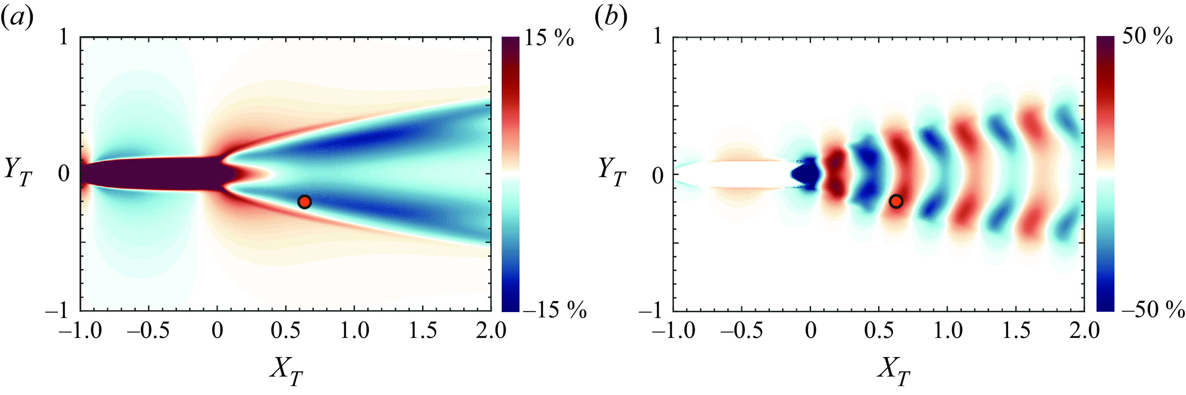
Time variation of $\bar {\alpha }_{\textit{eff}},\,\theta (t), \,\bar {\Lambda }_T$
, and
$\bar {\alpha }_{\textit{eff}},\,\theta (t), \,\bar {\Lambda }_T$
, and $\varDelta \bar {\Lambda }_T$
at the location d indicted in figure 6. Here, ‘TF’ and ‘SF’ represent ‘trailing fish’ and ‘solitary fish’, respectively. Downstroke and upstroke periods are marked on each plot.
$\varDelta \bar {\Lambda }_T$
at the location d indicted in figure 6. Here, ‘TF’ and ‘SF’ represent ‘trailing fish’ and ‘solitary fish’, respectively. Downstroke and upstroke periods are marked on each plot.
The plot of $\bar {\alpha }_{\textit{eff}}(t)$
for a TF shows some interesting differences from that of a SF. The entire curve for this quantity is essentially shifted downwards by values ranging from
$\bar {\alpha }_{\textit{eff}}(t)$
for a TF shows some interesting differences from that of a SF. The entire curve for this quantity is essentially shifted downwards by values ranging from $2^\circ$
to
$2^\circ$
to $10^\circ$
. We note that at this location
$10^\circ$
. We note that at this location $(\bar {u}_L,\bar {v}_L)=(1.045U, -0.168U)$
and this induces a flow angle of
$(\bar {u}_L,\bar {v}_L)=(1.045U, -0.168U)$
and this induces a flow angle of $-9^\circ$
, which is consistent with the shift in
$-9^\circ$
, which is consistent with the shift in $\bar {\alpha }_{\textit{eff}}(t)$
. This downwards lateral velocity at this location increases the effective angle of attack during the upstroke, but reduces the effective angle of attack during the downstroke, which is akin to the fin flapping with a biased pitch angle.
$\bar {\alpha }_{\textit{eff}}(t)$
. This downwards lateral velocity at this location increases the effective angle of attack during the upstroke, but reduces the effective angle of attack during the downstroke, which is akin to the fin flapping with a biased pitch angle.
Figure 10(b) shows the variation of $\sin ({\theta (t)}) \cdot \sin {(\alpha _{\textit{eff}}(t))}$
for these two cases and we note that, compared with the SF, the TF sees a significant reduction in this quantity during the downstroke and a smaller increase during the upstroke. This asymmetry is due to the fact that the downward shift of
$\sin ({\theta (t)}) \cdot \sin {(\alpha _{\textit{eff}}(t))}$
for these two cases and we note that, compared with the SF, the TF sees a significant reduction in this quantity during the downstroke and a smaller increase during the upstroke. This asymmetry is due to the fact that the downward shift of $\bar {\alpha }_{\textit{eff}}(t)$
results in a phase mismatch with
$\bar {\alpha }_{\textit{eff}}(t)$
results in a phase mismatch with $\theta (t)$
, thereby diminishing the product of these two functions. Thus, the net result of the mean wake is to reduce the thrust of the TF. The fluctuation in the flow velocity has nearly equal potential to either increase or decrease the thrust depending on the location. However, the negative bias effect due to the mean flow results in detrimental interactions being more significant.
$\theta (t)$
, thereby diminishing the product of these two functions. Thus, the net result of the mean wake is to reduce the thrust of the TF. The fluctuation in the flow velocity has nearly equal potential to either increase or decrease the thrust depending on the location. However, the negative bias effect due to the mean flow results in detrimental interactions being more significant.
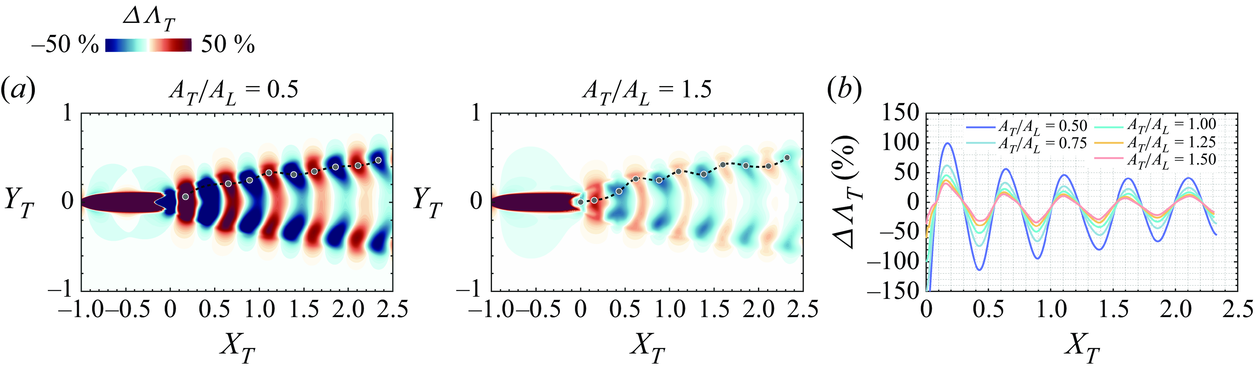
3.2.5. Influence of trailing fish tailbeat amplitude on thrust enhancement
In the previous section, we examined the case where the leading and TF swim with identical kinematics (i.e. the same amplitude and frequency). For these cases, the hydrodynamic interaction effects are determined almost exclusively by $\varDelta \phi _{\textit{eff}}$
, which depends on a combination of the difference in tail-beat phases and the distance between the two fish. However, depending on its position in the wake, a swimmer in the wake of a leading swimmer will experience changes in thrust (and therefore the total surge force), which would lead to acceleration or deceleration of the swimmer. One way to maintain the position at a beneficial location or to move from a detrimental position to a beneficial position is via modification in tailbeat amplitude. Indeed, a swimmer in a beneficial location could reduce their power expenditure while maintaining position by reducing their tailbeat amplitude. It is, therefore, of interest to examine the thrust enhancement map for a fish that is swimming in the wake of another fish using a tailbeat amplitude that is different from the leading fish. The current LEVBM provides the opportunity to easily examine this question since the kinematics of the TF can be modified without requiring any additional high-fidelity simulations.
$\varDelta \phi _{\textit{eff}}$
, which depends on a combination of the difference in tail-beat phases and the distance between the two fish. However, depending on its position in the wake, a swimmer in the wake of a leading swimmer will experience changes in thrust (and therefore the total surge force), which would lead to acceleration or deceleration of the swimmer. One way to maintain the position at a beneficial location or to move from a detrimental position to a beneficial position is via modification in tailbeat amplitude. Indeed, a swimmer in a beneficial location could reduce their power expenditure while maintaining position by reducing their tailbeat amplitude. It is, therefore, of interest to examine the thrust enhancement map for a fish that is swimming in the wake of another fish using a tailbeat amplitude that is different from the leading fish. The current LEVBM provides the opportunity to easily examine this question since the kinematics of the TF can be modified without requiring any additional high-fidelity simulations.
Figure 11 shows the effect of the tail-beat amplitude of the TF on thrust enhancement for the TF. The $\varDelta \Lambda _T$
maps for
$\varDelta \Lambda _T$
maps for $A_T/A_L = 0.5$
and
$A_T/A_L = 0.5$
and $A_T/A_L = 1.5$
reveal that the topology of the thrust enhancement map is similar to that for the same amplitude but a smaller flapping amplitude in the TF (
$A_T/A_L = 1.5$
reveal that the topology of the thrust enhancement map is similar to that for the same amplitude but a smaller flapping amplitude in the TF ( $A_T/A_L=0.5$
) leads to larger relative percentage increase in the
$A_T/A_L=0.5$
) leads to larger relative percentage increase in the $\varDelta \Lambda _T$
values. This is expected since for a TF with a reduced tail-beat amplitude, the wake perturbations
$\varDelta \Lambda _T$
values. This is expected since for a TF with a reduced tail-beat amplitude, the wake perturbations $(u^\prime _L,v^\prime _L)$
from the leading fish’s wake are more significant relative to the TF’s fin velocity, which is itself proportional to
$(u^\prime _L,v^\prime _L)$
from the leading fish’s wake are more significant relative to the TF’s fin velocity, which is itself proportional to $\dot {h}_T$
. Consequently, the effective angle of attack is modified more significantly by the wake interaction, leading to greater changes in
$\dot {h}_T$
. Consequently, the effective angle of attack is modified more significantly by the wake interaction, leading to greater changes in $\varDelta \Lambda _T$
. Conversely, with higher tail-beat amplitudes, the TF’s fin motion dominates, thereby reducing the influence of the perturbation from the wake vortices. Thus, the current analysis shows that a difference in amplitude between the two fish does not fundamentally change the flow physics of thrust enhancement, and this can serve as a viable strategy for maintaining or reaching a beneficial location in the wake.
$\varDelta \Lambda _T$
. Conversely, with higher tail-beat amplitudes, the TF’s fin motion dominates, thereby reducing the influence of the perturbation from the wake vortices. Thus, the current analysis shows that a difference in amplitude between the two fish does not fundamentally change the flow physics of thrust enhancement, and this can serve as a viable strategy for maintaining or reaching a beneficial location in the wake.
The $\varDelta \Lambda _T$
maps for two-fish schooling with different tailbeat amplitudes. (a) The
$\varDelta \Lambda _T$
maps for two-fish schooling with different tailbeat amplitudes. (a) The $\varDelta \Lambda _T$
maps for two different tailbeat amplitude,
$\varDelta \Lambda _T$
maps for two different tailbeat amplitude, $A,$
of the TF. (b) Presents
$A,$
of the TF. (b) Presents $\varDelta \Lambda _T$
values along curves connecting peaks and valleys on contours of corresponding
$\varDelta \Lambda _T$
values along curves connecting peaks and valleys on contours of corresponding $\varDelta \Lambda _T$
maps, demonstrated as grey dots and dashed lines in (a). These profiles highlight variations in
$\varDelta \Lambda _T$
maps, demonstrated as grey dots and dashed lines in (a). These profiles highlight variations in $\varDelta \Lambda _T$
along the streamwise direction
$\varDelta \Lambda _T$
along the streamwise direction $(X_T)$
, illustrating how amplitude influences the thrust generation.
$(X_T)$
, illustrating how amplitude influences the thrust generation.
3.2.6. Effect of Reynolds number
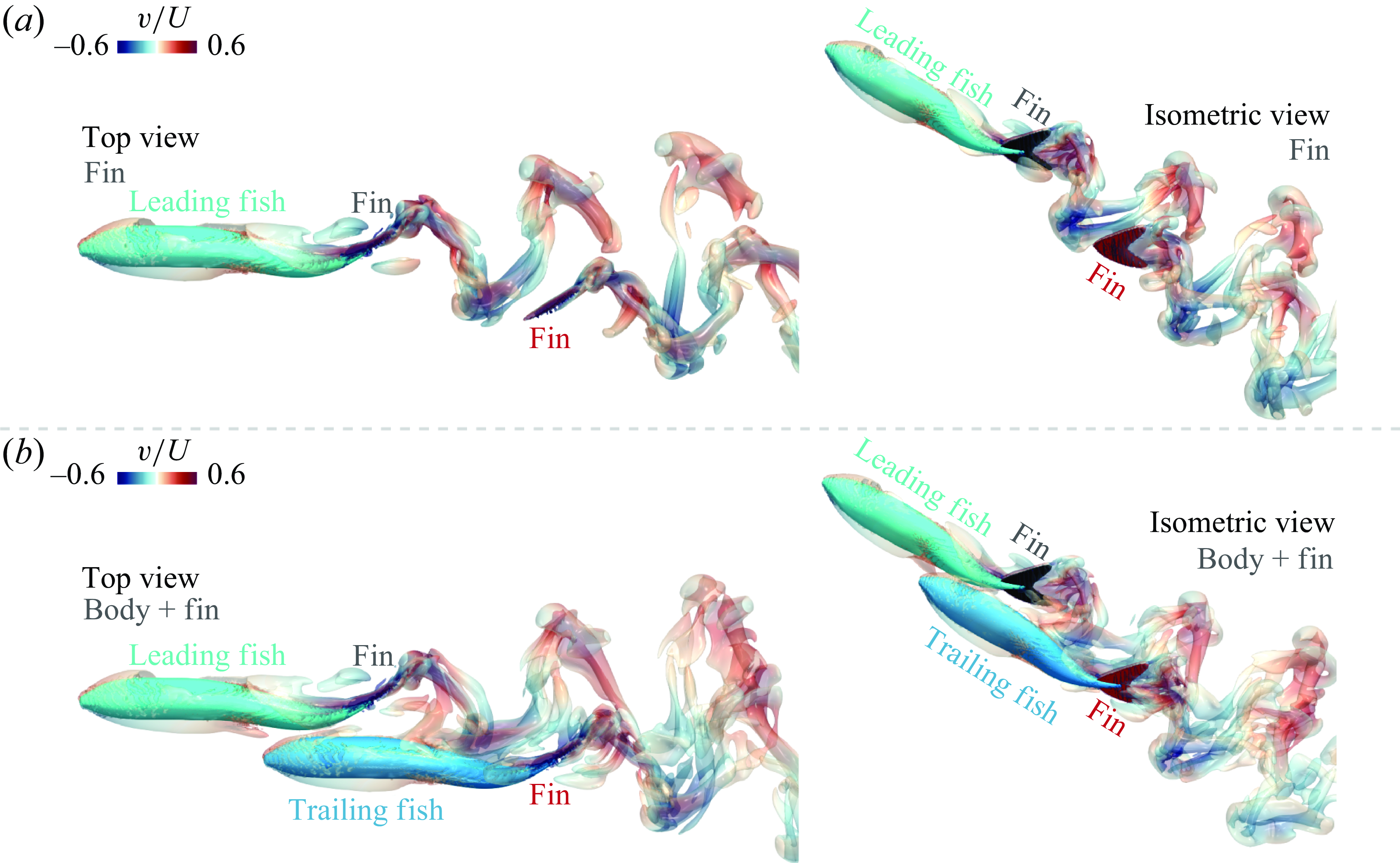
A Reynolds number of 5000 corresponds to a 2–5 cm caudal fin swimmer (such as a giant danio) swimming at O(1) BL s−1 (body length per second), and as we have seen that the wake at these low Reynolds number is well organised and highly periodic. It is of interest to see if the thrust enhancement maps are affected by an increase in Reynolds numbers, which would result in a complex, non-periodic wake with transitional/turbulent flow characteristics. To examine this, we employ our solver to compute the flow past the swimmer at a Reynolds number of 50 000. These simulations are carried out on a dense 233 million point grid, which was chosen after a grid convergence study (Mittal et al. Reference Mittal, Seo, Turner, Kumar, Prakhar and Zhou2025). To simulate a condition corresponding to steady swimming at a terminal speed, we have conducted a series of simulations at different free-stream velocities and selected a velocity for which the mean thrust and drag are nearly balanced out, and the net mean hydrodynamic force on the swimmer is almost zero. This condition for Re = 50 000 corresponds to a Strouhal number of 0.28, and it nominally represents a 15–20 cm carangiform swimmer such as a medium-sized trout. Note that the shear drag on the body of the fish reduces with increasing Reynolds number, thereby increasing the terminal speed (and reducing the Strouhal number) of the fish for a given tail-beat amplitude.
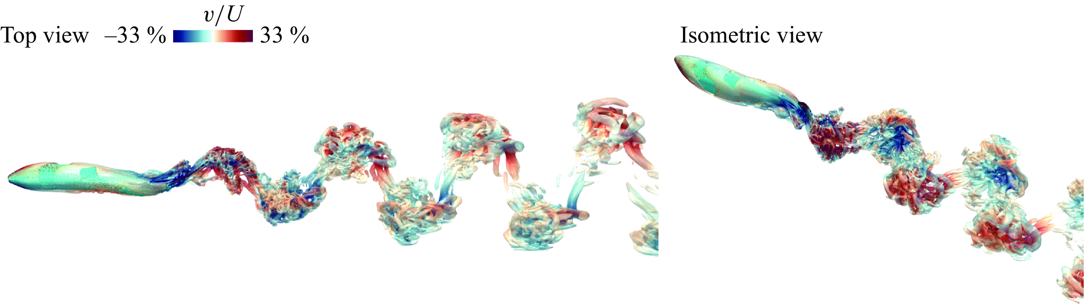
Figure 12 shows two views of the vortex structures in the wake, and we note that while the wake still exhibits the characteristic oblique dual-vortex street structure, the flow is significantly more complicated with a wide range of smaller vortex structures that are a result of various instabilities in the wake.
Instantaneous three-dimensional vortex structure of SF swimming at Re = 50 000. Structures are visualised by the iso-surface of $Q/f^2 = 1$
, coloured by the lateral velocity,
$Q/f^2 = 1$
, coloured by the lateral velocity, $v/U$
.
$v/U$
.
This lack of strict periodicity in the wake could impact the ability of a trailing swimmer to harness the induced velocities from the wake to enhance its LEV and thrust. To examine this issue, the wake velocity field from this simulation is extracted and used to generate a thrust enhancement map of a swimmer in the wake. Figure 13(a) shows the thrust enhancement map for a swimmer that is swimming with kinematics and phases that are identical to the leading swimmer. Remarkably, we find that despite the one order of magnitude increase in the Reynolds number and the significantly increased complexity of the wake, the thrust enhancement map looks very similar in form to that at the lower Reynolds number.
The $\varDelta \Lambda _T$
map and time variations of
$\varDelta \Lambda _T$
map and time variations of $\alpha _{\textit{eff}}$
along with
$\alpha _{\textit{eff}}$
along with $\theta (t)$
of SF swimming at re = 50 000. (a) The
$\theta (t)$
of SF swimming at re = 50 000. (a) The $\varDelta \Lambda _T$
map. The red dot at
$\varDelta \Lambda _T$
map. The red dot at $(X_T,Y_T)=(0.95,-0.17)$
represents one location of peak values on this
$(X_T,Y_T)=(0.95,-0.17)$
represents one location of peak values on this $\varDelta \Lambda _T$
map. The region at the left of the green line is invalid if the trailing fish is the same size as the leading fish. (a) Time variations of
$\varDelta \Lambda _T$
map. The region at the left of the green line is invalid if the trailing fish is the same size as the leading fish. (a) Time variations of $\alpha _{\textit{eff}}$
and
$\alpha _{\textit{eff}}$
and $\theta (t)$
at the location marked in (a). ‘TF’ and ‘SF’ represent ‘trailing fish’ and ‘solitary fish’, respectively. Downstroke and upstroke periods are marked on the plot.
$\theta (t)$
at the location marked in (a). ‘TF’ and ‘SF’ represent ‘trailing fish’ and ‘solitary fish’, respectively. Downstroke and upstroke periods are marked on the plot.
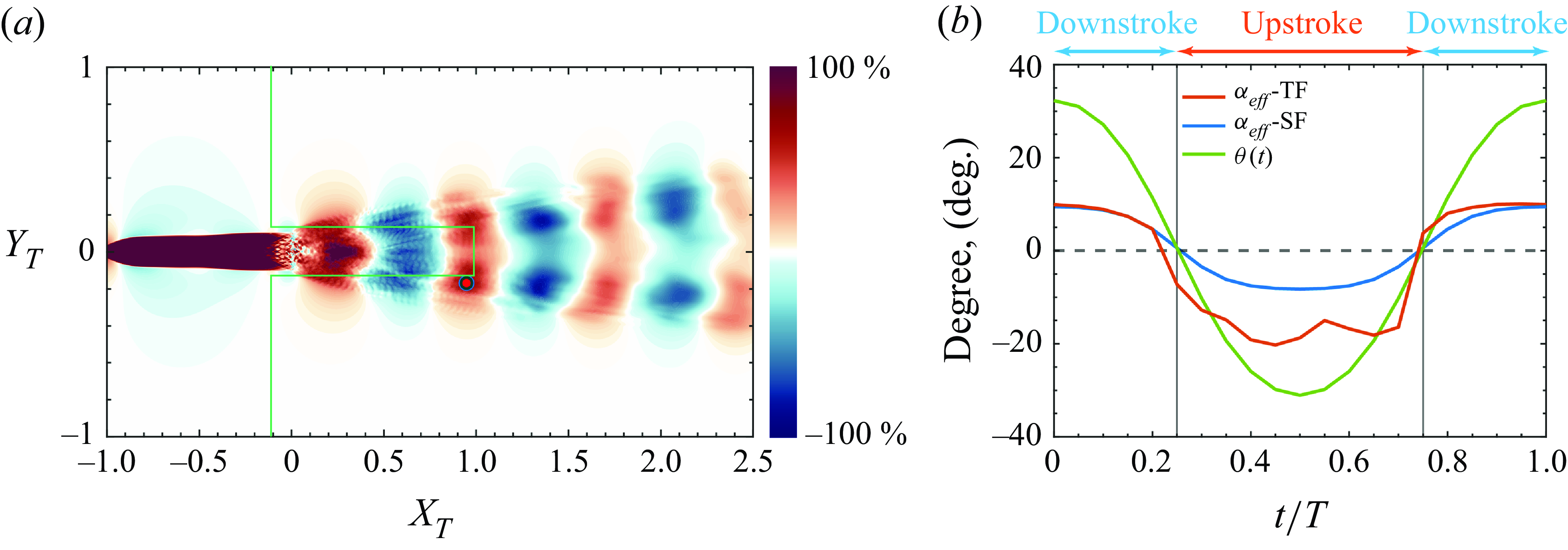
Figure 13(b) shows $\alpha _{\textit{eff}}$
for a TF at a beneficial location (marked in figure 13
a) along with the
$\alpha _{\textit{eff}}$
for a TF at a beneficial location (marked in figure 13
a) along with the $\alpha _{\textit{eff}}$
for a SF and
$\alpha _{\textit{eff}}$
for a SF and $\theta (t)$
. We observe from this figure that, while
$\theta (t)$
. We observe from this figure that, while $\alpha _{\textit{eff}}$
for the TF reflects the oscillatory and stochastic nature of the wake flow at this higher Reynolds number, there is an increase in the amplitude of this quantity, which ultimately results in a larger value of
$\alpha _{\textit{eff}}$
for the TF reflects the oscillatory and stochastic nature of the wake flow at this higher Reynolds number, there is an increase in the amplitude of this quantity, which ultimately results in a larger value of $\varDelta \Lambda _T$
at this location.
$\varDelta \Lambda _T$
at this location.
The two qualitative differences worth noting for the thrust maps at this higher Reynolds number are that first, the oblique angle of the thrust map pattern is slightly smaller than that at the lower Reynolds number shown in figure 7. The oblique angle of the vortex structures in the wake is related to the ratio of the lateral velocity imparted to the flow by the fin to the swimming speed, and this is directly proportional to the Strouhal number. The Strouhal number for the Re = 50 000 case is 0.28 compared with 0.42 for the Re = 5000 case, thereby explaining the difference in the oblique angles. Second, the streamwise wavelength of the thrust maps pattern is larger for the Re = 50 000 case, as compared with the Re = 5000 case (see figure 7). This wavelength is associated with the streamwise distance between the vortex structures generated in the wake by each fin flap and this wavelength is proportional to $(2A(x_F)/L)/$
St. Thus, the lower Strouhal number for the Re = 50 000 case explains the larger wavelength of the pattern for this case. At even lower Strouhal numbers which are seen for larger and/or faster swimming animals, these qualitative trends would be accentuated. All in all, this analysis indicates that the flow physics associated with wake-induced enhancement of the LEV is quite robust and effective for caudal fin swimmers over a large range of scales, and thus, the LEVBM based thrust maps will be applicable over this range of scales as well.
$(2A(x_F)/L)/$
St. Thus, the lower Strouhal number for the Re = 50 000 case explains the larger wavelength of the pattern for this case. At even lower Strouhal numbers which are seen for larger and/or faster swimming animals, these qualitative trends would be accentuated. All in all, this analysis indicates that the flow physics associated with wake-induced enhancement of the LEV is quite robust and effective for caudal fin swimmers over a large range of scales, and thus, the LEVBM based thrust maps will be applicable over this range of scales as well.
3.3. Extension to larger schools
3.3.1. Schools with three fish
Based on the successful demonstration of the use of $\varDelta \Lambda _T$
map for two-fish schools, we have applied the same methodology to predict beneficial configurations for three-fish schools, where the three are swimming with identical swimming strokes. For this, we first performed direct numerical simulations of two different optimal two-fish configurations, specifically
$\varDelta \Lambda _T$
map for two-fish schools, we have applied the same methodology to predict beneficial configurations for three-fish schools, where the three are swimming with identical swimming strokes. For this, we first performed direct numerical simulations of two different optimal two-fish configurations, specifically $a$
and
$a$
and $d$
in figure 6(b) and obtained their wake velocity fields. Using these velocity fields, beneficial locations for the third fish are explored by computing the respective
$d$
in figure 6(b) and obtained their wake velocity fields. Using these velocity fields, beneficial locations for the third fish are explored by computing the respective $\varDelta \Lambda _T$
maps (figure 14
a) for these cases. We note that there are many other two-fish configurations that could be examined, but we cannot explore all of them using DNS. The two configurations chosen here are, however, distinct enough that analysis of these two should provide general insights into the application of the LEVBM to larger fish schools.
$\varDelta \Lambda _T$
maps (figure 14
a) for these cases. We note that there are many other two-fish configurations that could be examined, but we cannot explore all of them using DNS. The two configurations chosen here are, however, distinct enough that analysis of these two should provide general insights into the application of the LEVBM to larger fish schools.
Predicted $\varDelta \Lambda _T$
map for the third fish in a three-fish school. (a) The
$\varDelta \Lambda _T$
map for the third fish in a three-fish school. (a) The $\varDelta \Lambda _T$
map indicating the optimal positions
$\varDelta \Lambda _T$
map indicating the optimal positions $(a, b, c, d, e)$
for a third fish in the wake of two leading fish with beneficial zones marked. The region to the left of the green line is invalid if the TF is the same size as the leading fish. (c) Direct numerical simulations of three-fish schools. Instantaneous three-dimensional vortex structures of three-fish schools corresponding to the optimal positions,
$(a, b, c, d, e)$
for a third fish in the wake of two leading fish with beneficial zones marked. The region to the left of the green line is invalid if the TF is the same size as the leading fish. (c) Direct numerical simulations of three-fish schools. Instantaneous three-dimensional vortex structures of three-fish schools corresponding to the optimal positions, $a{-}e$
, in (a). (c) Comparative plots of interactive effects (drag, thrust, power and efficiency) for each fish in configurations
$a{-}e$
, in (a). (c) Comparative plots of interactive effects (drag, thrust, power and efficiency) for each fish in configurations $(a, b, c, d, e)$
. Optimal positions, such as
$(a, b, c, d, e)$
. Optimal positions, such as $a$
and
$a$
and $b$
, enhance thrust and swimming efficiency for the third fish.
$b$
, enhance thrust and swimming efficiency for the third fish.
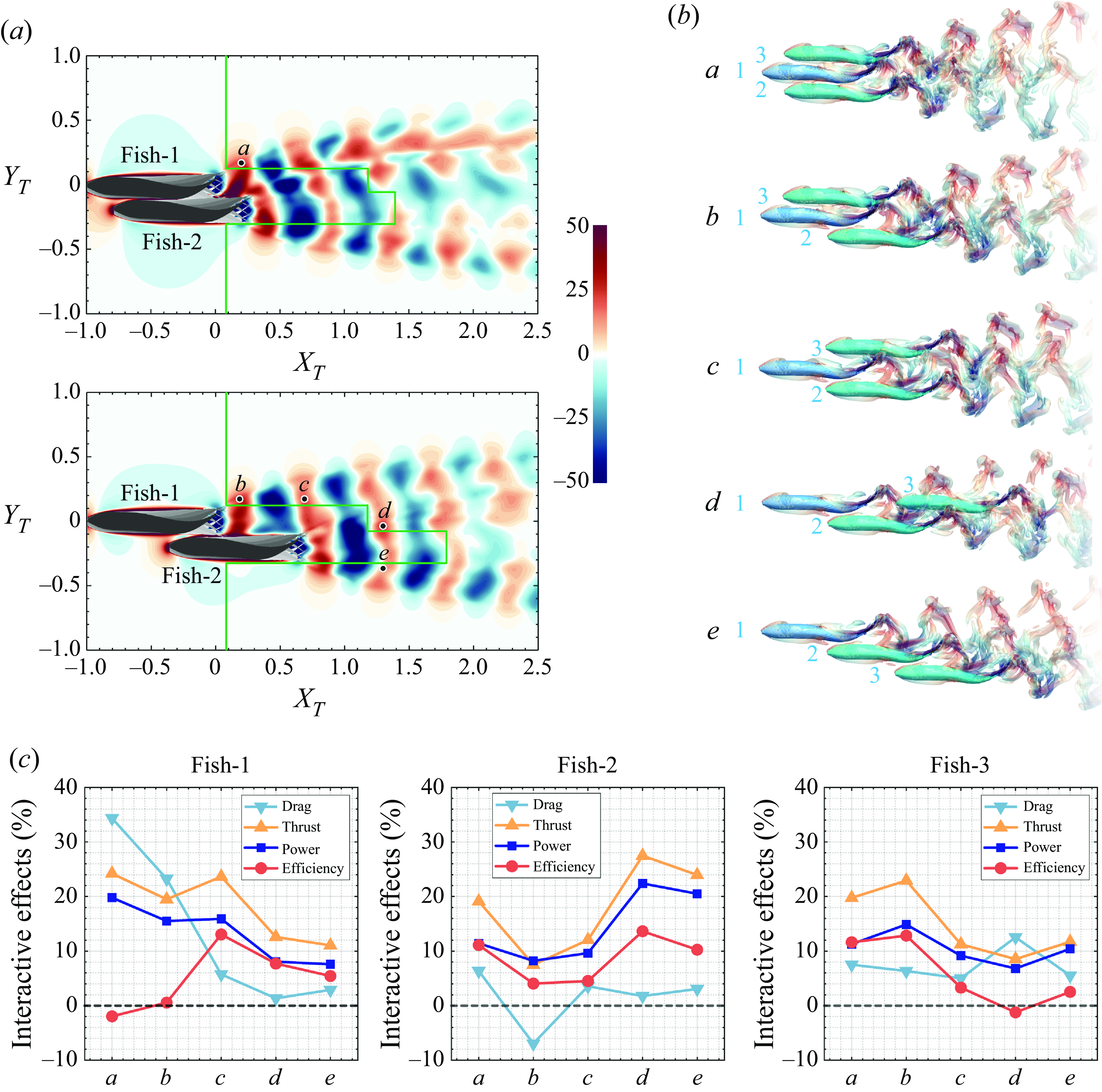
Figure 14(a) shows the thrust enhancement maps for the two two-fish configurations, and we note that, while the overall pattern of benefit and detriment is observed, the thrust enhancement maps have a significantly more complex topology. As shown in figure 14(a), the third fish can be positioned in many beneficial locations. We select five locations: 3-fish-a to 3-fish-e for a detailed analysis. Figure 14(b) illustrates the schematic of each configuration. Placing the third fish in position $a{-}c$
results in the well-documented diamond formation, which has been the subject of many previous studies (Pavlov & Kasumyan Reference Pavlov and Kasumyan2000; Liao Reference Liao2007; Timm et al. Reference Timm, Pandhare and Masoud2024). Alternatively, positioning the third fish at
$a{-}c$
results in the well-documented diamond formation, which has been the subject of many previous studies (Pavlov & Kasumyan Reference Pavlov and Kasumyan2000; Liao Reference Liao2007; Timm et al. Reference Timm, Pandhare and Masoud2024). Alternatively, positioning the third fish at $e$
leads to a diagonal configuration, theoretically allowing for further extension into larger schooling formations.
$e$
leads to a diagonal configuration, theoretically allowing for further extension into larger schooling formations.
To verify the configurations suggested by the $\varDelta \Lambda _T$
maps for the third fish, we have conducted DNS of those configurations illustrated in figure 14(b), and the metric related to the hydrodynamic performance of each swimmer is shown in figure 14(c). The availability of the DNS for these configurations allows us to perform a more comprehensive assessment of the swimming performance of the fish, including a quantification of the effect of schooling on drag, power and efficiency for all the fish in these configurations. We note that these additional quantities are unavailable from the LEVBM-based thrust enhancement maps.
$\varDelta \Lambda _T$
maps for the third fish, we have conducted DNS of those configurations illustrated in figure 14(b), and the metric related to the hydrodynamic performance of each swimmer is shown in figure 14(c). The availability of the DNS for these configurations allows us to perform a more comprehensive assessment of the swimming performance of the fish, including a quantification of the effect of schooling on drag, power and efficiency for all the fish in these configurations. We note that these additional quantities are unavailable from the LEVBM-based thrust enhancement maps.
The plots show that the thrust for every fish in all cases is enhanced, with the highest enhancement reaching 28 % ( $d$
, fish-2, in figure 14
c). Noticeably, as we selected specific beneficial configurations from optimal two-fish schools, fish-2, and even the leading fish, fish-1, still attain a distinct thrust enhancement in configurations
$d$
, fish-2, in figure 14
c). Noticeably, as we selected specific beneficial configurations from optimal two-fish schools, fish-2, and even the leading fish, fish-1, still attain a distinct thrust enhancement in configurations $a{-}e$
in figure 14(c). The interactive effects on drag reveal distinct trends depending on the swimmer’s position within the school. For the leading fish, fish-1, the drag increases significantly in compact configurations, such as
$a{-}e$
in figure 14(c). The interactive effects on drag reveal distinct trends depending on the swimmer’s position within the school. For the leading fish, fish-1, the drag increases significantly in compact configurations, such as $a$
. As the school becomes less compact (
$a$
. As the school becomes less compact ( $d$
and
$d$
and $e$
, for instance), the drag on fish-1 returns close to the baseline, highlighting the influence of the TF on the upstream flow dynamics. This observation underscores the fact that the TF can induce measurable hydrodynamic effects on the leading swimmer for compact configurations. In contrast, the drag changes for fish-2 and fish-3 are less pronounced, with variations remaining around 10 % across the various configurations. This suggests that the intermediate and trailing positions experience more stable drag conditions regardless of the compactness of the school.
$e$
, for instance), the drag on fish-1 returns close to the baseline, highlighting the influence of the TF on the upstream flow dynamics. This observation underscores the fact that the TF can induce measurable hydrodynamic effects on the leading swimmer for compact configurations. In contrast, the drag changes for fish-2 and fish-3 are less pronounced, with variations remaining around 10 % across the various configurations. This suggests that the intermediate and trailing positions experience more stable drag conditions regardless of the compactness of the school.
Fitting the LEVBM predictions to the corresponding thrust changes from DNS across cases ‘a’, ‘b’, ‘c’ and ‘e’, shows a linear relationship $\Delta T(\%) = 0.66\varDelta \Lambda _T(\%) + 0.02$
with a
$\Delta T(\%) = 0.66\varDelta \Lambda _T(\%) + 0.02$
with a $R^2$
value of 0.99. However, case ‘d’ deviates from this in that the DNS thrust increase is estimated to be 7.44%, whereas the LEVBM predicts a 30 % increase. This discordance arises because case ‘d’ is positioned within the wake of both leading fish, significantly increasing flow interactions with the body and introducing strong effects not accounted for in the LEVBM.
$R^2$
value of 0.99. However, case ‘d’ deviates from this in that the DNS thrust increase is estimated to be 7.44%, whereas the LEVBM predicts a 30 % increase. This discordance arises because case ‘d’ is positioned within the wake of both leading fish, significantly increasing flow interactions with the body and introducing strong effects not accounted for in the LEVBM.
The trend for power expenditure follows thrust, with increases observed for all fish in every configuration. The consistent alignment between thrust and power, combined with relatively stable drag changes, results in efficiency trends that follow similar patterns, except for fish-1. For fish-1, the significantly increased drag in configurations $a$
and
$a$
and $b$
negates the thrust gains, leading to an efficiency that is not much different from that of a SF. A similar effect is also observed for fish-3 in configuration
$b$
negates the thrust gains, leading to an efficiency that is not much different from that of a SF. A similar effect is also observed for fish-3 in configuration $d$
. Beyond these isolated effects, every configuration offers benefits in terms of improved thrust and efficiency for at least two of the three swimmers. Some configurations are particularly beneficial for one of the fish (for instance,
$d$
. Beyond these isolated effects, every configuration offers benefits in terms of improved thrust and efficiency for at least two of the three swimmers. Some configurations are particularly beneficial for one of the fish (for instance, $c$
for fish-1,
$c$
for fish-1, $d$
for fish-2 and
$d$
for fish-2 and $b$
for fish-3.
$b$
for fish-3.
In summary, these results demonstrate that the $\varDelta \Lambda _T$
map not only reliably predicts thrust improvements across different configurations but also shows that these thrust improvements, which are associated with the enhancement of LEV on the caudal fin, are also often accompanied by concurrent improvements in efficiency.
$\varDelta \Lambda _T$
map not only reliably predicts thrust improvements across different configurations but also shows that these thrust improvements, which are associated with the enhancement of LEV on the caudal fin, are also often accompanied by concurrent improvements in efficiency.
3.3.2. Application to larger schools
In the previous sections, we have shown how LEVBM-based thrust enhancement maps provide an understanding of the effect of relative location and phase for fish in small schools comprising up to 3 swimmers. We have also shown that these maps apply over a wide range of scales. The final question that we address is: Can these thrust enhancement maps apply to larger schools, or is the flow in larger schools so complicated that it would not lend itself to the relatively simple phenomenology that forms the basis of the LEVBM thrust enhancement maps?
To address this question, we consider two nine-fish schools that have been the subject of our previous study (Zhou et al. Reference Zhou, Seo and Mittal2023, Reference Zhou, Seo and Mittal2024). Each individual fish in these schools corresponds exactly to the configuration examined in § 3.1. In both schools, the fish are arranged exactly in the same tight diamond configuration, but in the first school, all nine fish are swimming with the same phase, and in the second school, fish in each row are swimming with a $0.5 \pi$
phase difference from the fish in the previous row. Thus, these two schools provide two significantly distinct configurations for the application of the LEVBM. Indeed, the plots of the vortex structures for these two schools (figure 15
a and b) confirm the fact that the wake flows for these two schools are not only very complex but also quite distinct.
$0.5 \pi$
phase difference from the fish in the previous row. Thus, these two schools provide two significantly distinct configurations for the application of the LEVBM. Indeed, the plots of the vortex structures for these two schools (figure 15
a and b) confirm the fact that the wake flows for these two schools are not only very complex but also quite distinct.
Direct numerical simulations of nine-fish school and the corresponding $\varDelta \Lambda _T$
maps for a fish trailing this school. Panels (a) and (b)Instantaneous three-dimensional vortex structure of the nine-fish schools with synchronised and de-synchronised phases, respectively. Structures are visualised by the iso-surface of
$\varDelta \Lambda _T$
maps for a fish trailing this school. Panels (a) and (b)Instantaneous three-dimensional vortex structure of the nine-fish schools with synchronised and de-synchronised phases, respectively. Structures are visualised by the iso-surface of $Q/f^2 = 1$
, coloured by the lateral velocity,
$Q/f^2 = 1$
, coloured by the lateral velocity, $v/U$
. Panels (c) and (d) show the
$v/U$
. Panels (c) and (d) show the $\varDelta \Lambda _T$
maps for nine-fish schools with synchronised and de-synchronised phases, respectively. Here,
$\varDelta \Lambda _T$
maps for nine-fish schools with synchronised and de-synchronised phases, respectively. Here, $\varDelta \phi =\phi _{10}-\phi _i$
, where
$\varDelta \phi =\phi _{10}-\phi _i$
, where $\phi _{10}$
is the phase of the tenth fish.
$\phi _{10}$
is the phase of the tenth fish.
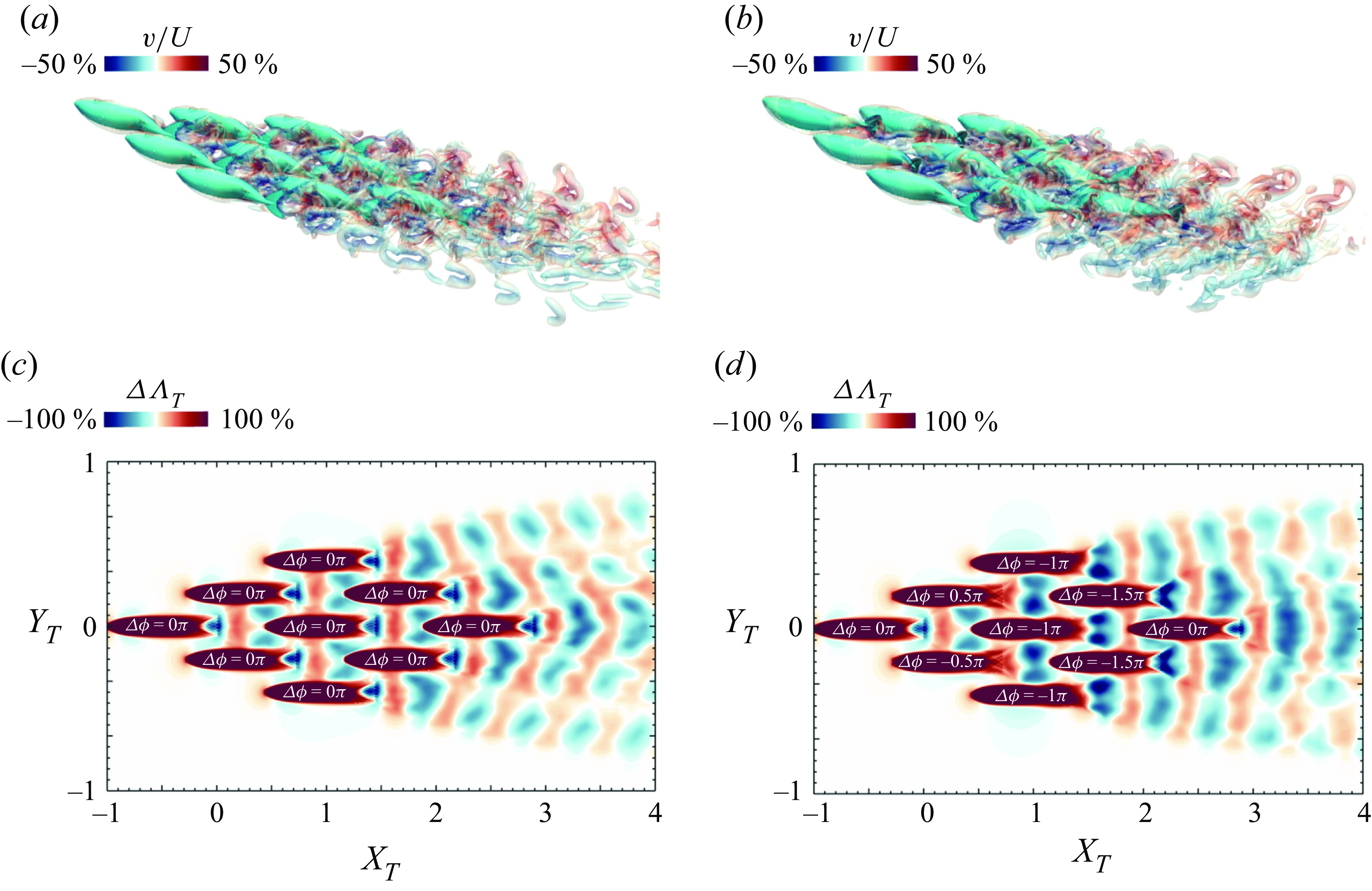
Thrust enhancement maps are computed for both these schools, and these are done for a TF swimming with identical kinematics and a fin flapping phase that matches that of the leading fish in the schools. Figure 15(c,d) shows the thrust enhancement maps for these two schools, and we observe that while the two maps are not identical, they exhibit a surprising similarity to each other and with the thrust enhancement maps for a single leading fish. In particular, both maps are dominated by laterally oriented alternating bands of thrust enhancement and decrement. Thus, despite the tremendous complexity of the vortex wake of the nine-fish schools, the effect on the thrust of a TF is quite similar to that for a single fish. The emergence of this simplicity from complexity is quite remarkable and connected with two facts: first, vortices from the various fish in the school tend to self-organise in banded structures due to mutual induction. This effect is visible in the vortex structure plots for the two schools. Second, the vorticity tends to highlight small-scale structures. However, the thrust enhancement is associated primarily with transverse velocity, which is still primarily driven by the sinusoidal movement of the caudal fin. This suggests that the model could be applied successfully to even larger schools but this is out of scope of the current study. The challenge with applying this to larger schools is that, in order to place a (N + 1)th fish in the wake of a ‘N’ fish school, one needs to conduct DNS of the N-fish school and obtain the wake for estimating the thrust map, and this is computationally expensive. Simpler methods for predicting the wake profiles of schools are needed to scale this methods to large schools.
4. Summary
The LEVBM-based thrust enhancement maps are shown to serve as a useful tool for investigating the hydrodynamics of fish schooling without incurring the high computational costs typically associated with direct numerical simulation. Unlike models based on idealised flow physics, the LEVBM-based thrust enhancement maps incorporate the essential effect of LEV formation (Seo & Mittal Reference Seo and Mittal2022) and a detailed validation of thrust enhancement maps against direct numerical simulations provide confidence that, despite its simplicity, the model provides a reasonable representation of the complex flow physics of thrust generation and enhancement associated with the LEV on the caudal fin. Leveraging the predictive capability of the model, we examined a large parameter space of locations, phase and undulation amplitudes and frequencies of the TF on its thrust enhancement. This kind of parameter sweep would not be possible using fully resolving simulations, and this capability enabled new insights into the hydrodynamics of fish schooling.
The following are the key findings of the study:
-
(i) For a trailing BCF swimmer swimming with kinematics identical to a leading BCF swimmer, there is a repeating pattern of locations in the near wake where it can derive propulsion benefits through hydrodynamic interactions with the wake of the leading fish. A change in the relative phase between the undulations of the two fish only generates a small streamwise shift in the pattern. Thus, spatial positioning and phase synchronisation in fish schools are interchangeable parameters for TF attempting to benefit from hydrodynamic interactions.
-
(ii) The thrust enhancement maps generated from the LEVBM cannot account for the effects of the body of the TF, but despite this, for slender-bodied swimmers such as those in the current study, the thrust enhancement maps still provide valuable predictions of the regions of thrust enhancement.
-
(iii) The thrust enhancement maps do not directly provide information regarding hydrodynamic efficiency, but the DNS show that improved thrust for the TF is almost always accompanied by concurrent improvements in hydrodynamic efficiency. This is consistent with the fact that, for the TF, improvements in thrust are a result of LEV enhancement due to hydrodynamic interactions, and this leveraging of kinetic energy from the wake of the leading fish to amplify the growth of the LEV is power efficient since it does not require any additional movement from the caudal fin.
-
(iv) An intriguing finding of the current study, corroborated by DNS, is that detrimental interactions (i.e. hydrodynamic interactions that reduce the thrust of the TF) are not only significant, but they, in fact, exceed the magnitude of beneficial interactions. Notably, there is an alternating pattern of thrust enhancement and decrement in the wake and the dominance of the detrimental interactions is traced to the effect of the large transverse component of induced velocity in the mean wake of the leading fish.
-
(v) Avoidance of regions of detrimental interactions could be as crucial in the formation of schools as seeking regions of thrust enhancement. Indeed, the presence of multiple locations in the parameter space of effective phase difference where the thrust is either increased or decreased would serve to drive dynamic changes in the relative position and swimming kinematics of the TF. Taken together, all of the features of the thrust enhancement map topology described in the previous two sections provide a possible explanation for why actual fish schools, including even small-scale schools in laboratory settings, exhibit highly complex and dynamic topologies, with the fish seldom staying in, what seem to be well-organised configurations (Tunström et al. Reference Tunström, Katz, Ioannou, Huepe, Lutz and Couzin2013; Peterson, Swanson & McHenry Reference Peterson, Swanson and McHenry2024; Zhang & Lauder Reference Zhang and Lauder2024). We note that the thrust maps also suggest a way for fish and bioinspired autonomous underwater vehicles (AUVs) to avoid these detrimental interactions – this could be done by the TF either changing its phase or location relative to the leading fish, or through a combination of the two.
-
(vi) A corollary to the analysis of the detrimental interaction predicted by the LEVBM-based thrust enhancement maps is that undulatory carangiform swimming naturally generates a flapping motion of the caudal fin where the time-varying pitch angle and effective angle of attack are in phase. As per the LEVBM, this condition is very well suited (one could even consider this ‘optimised’) for thrust generation. Past studies on engineered flapping foils allocated considerable effort to manually synthesise effective angle-of-attack profiles to achieve optimal propulsion (Read, Hover & Triantafyllou Reference Read, Hover and Triantafyllou2003; Hover, Haugsdal & Triantafyllou Reference Hover, Haugsdal and Triantafyllou2004). However, carangiform swimming of fish accomplishes this automatically, in what could be considered an elegant example of embodied intelligence resulting from millions of years of evolution.
-
(vii) We find that TF can swim with different undulatory amplitude than the leading fish and still reap the benefits of beneficial interactions in a manner similar to the case when the amplitudes are identical. Unsurprisingly, the relative increase in thrust decreases (increases) with increasing (decreasing) tail amplitude.
-
(viii) The thrust enhancement maps are mostly unchanged despite an order-of-magnitude increase in Reynolds number, suggesting a robustness in the LEV enhancement mechanism associated with thrust increase.
-
(ix) Although the detailed analysis in this study focused on small schools of two and three fish, the computation of thrust enhancement maps for two distinct nine-fish schools reveals a somewhat counterintuitive simplicity emerging from the complex individual wakes of the fish. This simplicity manifests as a repeating banded structure of thrust enhancement and reduction within the school’s wake, which is similar to that for a single fish. These findings have intriguing implications for fish schooling, suggesting that extracting hydrodynamic benefits from the wakes of leading fish does not necessarily become more challenging as the school size increases. Similarly, this has significant implications for bio-inspired AUVs, indicating that large ’schools’ of such AUVs could exploit wake interactions to lower energy consumption and extend operational endurance, without requiring complex sensing and control strategies. The results from this study offer a foundation for designing and testing such systems, with the LEVBM serving as a guideline for optimising the spacing and synchronisation of AUV formations.
4.1. Limitations and future work
Several limitations of the study should be acknowledged. First, the simulations were conducted under idealised conditions, where the flow was assumed to be laminar, and the tethered fish maintained constant swimming speeds. In real-world scenarios, fish often swim in turbulent environments with fluctuating flow conditions. Incorporating turbulence into future models would provide a more realistic assessment of the hydrodynamic interactions in fish schools. Additionally, the present study focused on BCF swimmers, with most of the thrust coming from the caudal fin. Future work should consider multiple fins and a flexible body dynamics to better capture the full spectrum of hydrodynamic interactions, especially for other swimming modes.
Finally, the biological implications of these hydrodynamic findings remain to be fully explored. While the $\varDelta \Lambda _T$
map provides trustworthy predictions for thrust generation, fish schools will likely optimise for multiple objectives simultaneously, including predator avoidance, stability and information exchange. Investigating how these factors interact with the hydrodynamics could enrich our understanding of fish schooling behaviour. The current study has a focus on sinusoidal swimming motion whereas fish, especially those swimming in schools, might employ unsteady and intermittent swimming. The current model can, in principle, be extended for these situations but this will require additional work to cover a vastly larger parameter space and to verify the model predictions.
$\varDelta \Lambda _T$
map provides trustworthy predictions for thrust generation, fish schools will likely optimise for multiple objectives simultaneously, including predator avoidance, stability and information exchange. Investigating how these factors interact with the hydrodynamics could enrich our understanding of fish schooling behaviour. The current study has a focus on sinusoidal swimming motion whereas fish, especially those swimming in schools, might employ unsteady and intermittent swimming. The current model can, in principle, be extended for these situations but this will require additional work to cover a vastly larger parameter space and to verify the model predictions.
Funding
This work is supported by ONR Grants N00014-22-1-2655 and N00014-22-1-2770 monitored by Dr. Robert Brizzolara. This work used the computational resources at the Advanced Research Computing at Hopkins (ARCH) core facility (rockfish.jhu.edu), which is supported by the AFOSR DURIP Grant FA9550-21-1-0303, and the Extreme Science and Engineering Discovery Environment (XSEDE), which is supported by National Science Foundation Grant No. ACI-1 548 562, through allocation number TG-CTS100002.
Declaration of interests
The authors report no conflict of interest.
Appendix A. Hydrodynamic Metrics
The force and mechanical power are computed as follows through surface integrals
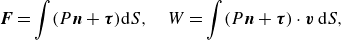 \begin{equation} {\boldsymbol{F}} = \int (P {\boldsymbol{n}} + {\boldsymbol{\tau }})\text{d}S, \quad W = \int (P {\boldsymbol{n}} + {\boldsymbol{\tau }}) \cdot {\boldsymbol{v}} \, \text{d}S, \end{equation}
where ${\boldsymbol{n}}$
is the normal unit vector pointing inside the body surface,
${\boldsymbol{n}}$
is the normal unit vector pointing inside the body surface, ${\boldsymbol{\tau }}$
and
${\boldsymbol{\tau }}$
and ${\boldsymbol{v}}$
are the viscous stress and body velocity on the surface, respectively. Changes in force and power are defined as
${\boldsymbol{v}}$
are the viscous stress and body velocity on the surface, respectively. Changes in force and power are defined as
 \begin{equation} \Delta F_{{D}} = F_{{D}} - F_{{D, solitary}}, \quad \Delta F_{{T}} = F_{{T}} - F_{{T,solitary}}, \quad \Delta W = W - W_{{solitary}}, \end{equation}
where $F_{{D}}$
and
$F_{{D}}$
and $F_{{T}}$
are the mean drag and thrust, calculated using the surface integral (A1) on the body and the fin in the streamwise direction, respectively. We use the Froude efficiency (Liu et al. Reference Liu, Ren, Dong, Akanyeti, Liao and Lauder2017; Zhou & Mittal Reference Zhou and Mittal2018) (
$F_{{T}}$
are the mean drag and thrust, calculated using the surface integral (A1) on the body and the fin in the streamwise direction, respectively. We use the Froude efficiency (Liu et al. Reference Liu, Ren, Dong, Akanyeti, Liao and Lauder2017; Zhou & Mittal Reference Zhou and Mittal2018) ( $\eta$
) to quantify the hydrodynamic efficiency and the difference referring to SF swimming
$\eta$
) to quantify the hydrodynamic efficiency and the difference referring to SF swimming
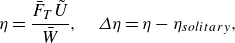 \begin{equation} \eta = \frac {\bar {F}_{{T}} \tilde {U}}{\bar {W}}, \quad \varDelta \eta = \eta - \eta _{{solitary}}, \end{equation}
where $\bar {F}_{{T}}$
and
$\bar {F}_{{T}}$
and $\bar {W}$
represent averaged thrust and power. The parameter
$\bar {W}$
represent averaged thrust and power. The parameter $\tilde {U}$
is the adjusted swimming velocity defined as
$\tilde {U}$
is the adjusted swimming velocity defined as
 \begin{equation} \tilde {U} = U + (\text{d}U/\text{d}F) \Delta F_{{net}}, \quad \Delta F_{{net}} = \Delta F_{{T}} - \Delta F_{{D}}. \end{equation}
To correctly quantify the interactive effects, we use $\tilde {U}$
to adjust the change in drag due to the hydrodynamic interaction. The
$\tilde {U}$
to adjust the change in drag due to the hydrodynamic interaction. The $(\text{d}U/\text{d}F)$
is obtained from the SF simulations, whose Froude efficiency is 34 %, matching previous studies (Borazjani & Daghooghi Reference Borazjani and Daghooghi2013; Daghooghi & Borazjani Reference Daghooghi and Borazjani2015).
$(\text{d}U/\text{d}F)$
is obtained from the SF simulations, whose Froude efficiency is 34 %, matching previous studies (Borazjani & Daghooghi Reference Borazjani and Daghooghi2013; Daghooghi & Borazjani Reference Daghooghi and Borazjani2015).


 Open access