1 Introduction
1.1 About these notes
These lecture notes expand (significantly) on a two hour tutorial given at the 2017 Les Houches school ‘From laboratories to astrophysics: the expanding universe of plasma physics’. Many excellent books and reviews have already been written on the subjects of dynamo theory, planetary and astrophysical magnetism. Most of them, however, are either quite specialised, or simply too advanced for non-specialists seeking a general entry point into the field. The multidisciplinary context of this school, taking place almost a century after Larmor’s original idea of self-exciting fluid dynamos, provided an ideal opportunity to craft a self-contained, wide ranging, yet relatively accessible introduction to the subject.
One of my central preoccupations in the writing process has been to attempt to distil in clear and relatively concise terms the essence of each of the problems covered, and to highlight to the best of my abilities the successes, limitations and connections of different lines of research in logical order. Although I may not have entirely succeeded, my sincere hope is that this review will nevertheless turn out to be generally useful to observers, experimentalists, theoreticians, PhD students, newcomers and established researchers in the field alike, and will foster new original research on dynamos of all kinds. It is quite inevitable, though, that such an ideal can only be sought at the expense of total exhaustivity and mathematical rigour, and necessitates making difficult editorial choices. To borrow Keith Moffatt’s wise words in the introduction of his 1973 Les Houches lecture notes on fluid dynamics and dynamos, ‘it will be evident that in the time available I have had to skate over certain difficult topics with indecent haste. I hope however that I have succeeded in conveying something of the excitement of current research in dynamo theory and something of the general flavour of the subject. Those already acquainted with the subject will know that my account is woefully one-sided’. Suggestions for further reading on the many different branches of dynamo research discussed in the text are provided throughout the document and in appendix A to mitigate these limitations.
Finally, while the main focus of the notes is on the physical and practical mathematical aspects of dynamo theory in general, contextual information is provided throughout to connect the material presented to astrophysical, geophysical and experimental dynamo problems. In particular, a selection of astrophysical and planetary dynamo research topics, including the geo-, solar and accretion-disc dynamos, is highlighted in the most advanced parts of the review to give a flavour of the diversity of research and challenges in the field.
1.2 Observational roots of dynamo theory
Dynamo theory finds its roots in the human observation of the Universe, and in the quest to understand the origin of magnetic fields observed or inferred in a variety of astrophysical systems. This includes planetary magnetism (the Earth, other planets and their satellites), solar and stellar magnetism and cosmic magnetism (galaxies, clusters and the Universe as a whole). We will therefore start with a brief overview of the main features of astrophysical and planetary magnetism.
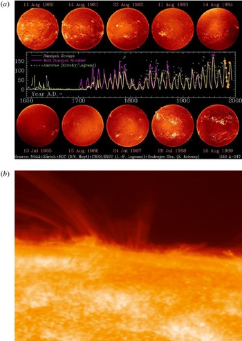
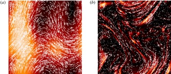
(a) Large-scale solar magnetism. The eleven year magnetic solar cycle (#21–22) observed in the chromosphere through the H $\unicode[STIX]{x1D6FC}$
spectral line (full solar discs), and historical sunspot-number record (Credits: NOAA/Zürich/RDC/CNRS/INSU/Ondresjov Observatory/HAO). (b) Local and global solar magnetic dynamics. The rapidly evolving small-scale magnetic carpet, spicules and sunspot arches imaged near the limb in the lower chromosphere through the CaH spectral line (Credits: SOT/Hinode/JAXA/NASA).
$\unicode[STIX]{x1D6FC}$
spectral line (full solar discs), and historical sunspot-number record (Credits: NOAA/Zürich/RDC/CNRS/INSU/Ondresjov Observatory/HAO). (b) Local and global solar magnetic dynamics. The rapidly evolving small-scale magnetic carpet, spicules and sunspot arches imaged near the limb in the lower chromosphere through the CaH spectral line (Credits: SOT/Hinode/JAXA/NASA).

Consider first solar magnetism, whose evolution on human time scales and day-to-day monitoring make it a more intuitive dynamical phenomenon to apprehend than other forms of astrophysical magnetism. For the purpose of the discussion, we can single out two ‘easily’ observable dynamical magnetic time scales on the Sun. The first one is the eleven year magnetic cycle time scale over which the large-scale solar magnetic field reverses. The solar cycle shows up in many different observational records, the most well known of which is probably the number of sunspots as a function of time, see figure 1(a) (note that the eleven year cycle is also chaotically modulated on longer time scales). Large-scale solar magnetism is characterised by an average (mean) field of only a few tens of Gauss (see e.g. the review by Charbonneau Reference Charbonneau2014), however the field itself can exceed kiloGauss strengths in large-scale features like sunspots.Footnote 1 There is also a lot of dynamical, small-scale, disordered magnetism in the solar surface photosphere and chromosphere, evolving on short time and spatial scales comparable to those of thermal convective motions at the surface (from a minute to an hour, and from a few kilometres to a few thousands of kilometres). This so-called ‘network’ and ‘internetwork’ small-scale magnetism, depicted in figure 1(b), was discovered much more recently (Livingston & Harvey Reference Livingston, Harvey and Howard1971). Its typical strength ranges from a few to a few hundred Gauss, and does not appear to be significantly modulated over the course of the global solar cycle (see e.g. Solanki, Inhester & Schüssler Reference Solanki, Inhester and Schüssler2006; Stenflo Reference Stenflo2013, for reviews). Large-scale stellar magnetic fields, including time-dependent ones, have been detected on many other stars (e.g. Donati & Landstreet Reference Donati and Landstreet2009), but only for the Sun do we have accurate, temporally and spatially resolved direct measurements of small-scale stellar magnetism.
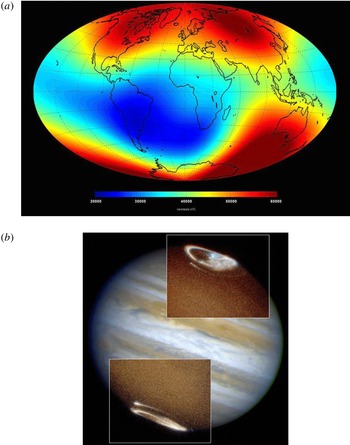
(a) Direct satellite measurements of the Earth’s magnetic-field strength (in nano Teslas) in 2014 at an altitude of 450 km (Credits: Swarm/CNES/ESA). (b) Ultra-violet emission of a 1998 Jupiter aurora (Credits: J. Clarke/STIS/WFPC2/HST/NASA/ESA).

The second major natural, human-felt phenomenon that inspired the development of dynamo theory is of course the Earth’s magnetic field, whose strength at the surface of the Earth is of the order of 0.1 Gauss ( $10^{-5}$
T, Finlay et al.
Reference Finlay, Maus, Beggan, Bondar, Chambodut, Chernova, Chulliat, Golovkov, Hamilton and Hamoudi2010). The dynamical evolution and structure of the field, including its many irregular reversals over a hundred-thousand to million year time scale, is established through paleomagnetic and archeomagnetic records, marine navigation books and is now monitored with satellites, as shown in figure 2(a). While the terrestrial field is probably highly multiscale and multipolar in the liquid iron part of the core where it is generated, it is primarily considered as a form of large-scale dynamical magnetism involving a north and south magnetic pole. Several other planets of the solar system also exhibit large-scale, low-multipole surface magnetic fields and magnetospheres. Figure 2(b) shows auroral emissions on Jupiter, whose magnetic field has a typical surface strength of a few Gauss (a few
$10^{-5}$
T, Finlay et al.
Reference Finlay, Maus, Beggan, Bondar, Chambodut, Chernova, Chulliat, Golovkov, Hamilton and Hamoudi2010). The dynamical evolution and structure of the field, including its many irregular reversals over a hundred-thousand to million year time scale, is established through paleomagnetic and archeomagnetic records, marine navigation books and is now monitored with satellites, as shown in figure 2(a). While the terrestrial field is probably highly multiscale and multipolar in the liquid iron part of the core where it is generated, it is primarily considered as a form of large-scale dynamical magnetism involving a north and south magnetic pole. Several other planets of the solar system also exhibit large-scale, low-multipole surface magnetic fields and magnetospheres. Figure 2(b) shows auroral emissions on Jupiter, whose magnetic field has a typical surface strength of a few Gauss (a few $10^{-4}$
T, Khurana et al.
Reference Khurana, Kivelson, Vasyliunas, Krupp, Woch, Lagg, Mauk, Kurth, Bagenal, Dowling and McKinnon2004). Just as in the Earth’s case, the large-scale external field of the other magnetic planets is almost certainly not representative of the structure of the field in the interior.
$10^{-4}$
T, Khurana et al.
Reference Khurana, Kivelson, Vasyliunas, Krupp, Woch, Lagg, Mauk, Kurth, Bagenal, Dowling and McKinnon2004). Just as in the Earth’s case, the large-scale external field of the other magnetic planets is almost certainly not representative of the structure of the field in the interior.
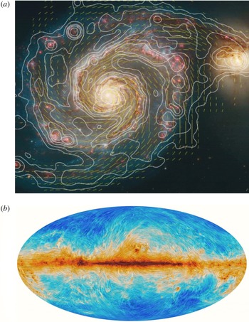
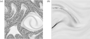
(a) Large-scale spiral magnetic structure (line segments) of the M51 galaxy established from radio observations of polarised synchrotron emission by cosmic rays (Credits: MPIfR Bonn and Hubble Heritage Team. Graphics: Sterne and Weltraum). (b) Map of the microwave galactic dust emission convolved with galactic magnetic-field lines reconstructed from polarisation maps of the dust emission (Credits: M. A. Miville-Deschênes/CNRS/ESA/Planck collaboration).

Moving further away from the Earth, we also learned in the second part of the twentieth century that galaxies, including our own Milky Way, host magnetic fields with a typical strength of the order of a few $10^{-5}$
Gauss (Beck & Wielebinski Reference Beck, Wielebinski, Oswalt and Gilmore2013). For a long time, observations would only reveal the ordered large-scale, global magnetic structure whose projection in the galactic plane would often take the form of spirals, see figure 3(a). But recent high-resolution observations of polarised dust emission in our galaxy, displayed in figure 3(b), have now also established that the galactic magnetic field has a very intricate multiscale structure, of which a large-scale ordered field is just one component.
$10^{-5}$
Gauss (Beck & Wielebinski Reference Beck, Wielebinski, Oswalt and Gilmore2013). For a long time, observations would only reveal the ordered large-scale, global magnetic structure whose projection in the galactic plane would often take the form of spirals, see figure 3(a). But recent high-resolution observations of polarised dust emission in our galaxy, displayed in figure 3(b), have now also established that the galactic magnetic field has a very intricate multiscale structure, of which a large-scale ordered field is just one component.
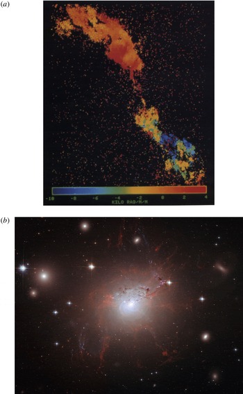
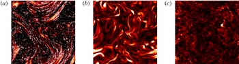
(a) Faraday rotation measure map (a proxy for the line-of-sight component of the magnetic field) in the synchrotron-illuminated radio lobes of the Hydra A cluster (Credits: Taylor & Perley/VLA/NRAO). (b) Visible-light observations of magnetised filaments in the core of the Perseus cluster (Credits: Fabian et al./HST/ESA/NASA).

Magnetic fields of the order of a few $10^{-6}$
Gauss are also measured in the hot intracluster medium (ICM) of galaxy clusters (e.g. Carilli & Taylor Reference Carilli and Taylor2002; Bonafede et al.
Reference Bonafede, Feretti, Murgia, Govoni, Giovannini, Dallacasa, Dolag and Taylor2010). The large-scale global structure and orientation of cluster fields, if any, is not well determined (it should be noted in this respect that global differential rotation is not thought to be very important in clusters, unlike in individual galaxies, stars and planets). On the other hand, synchrotron polarimetry measurements in the radio lobes of active galactic nuclei (AGN), such as that shown in figure 4(a), suggest that there is a significant ‘small-scale’, turbulent ICM field component on scales comparable to or even smaller than a kiloparsec (Vogt & Ensslin Reference Vogt and Ensslin2005). Visible-light observations of the ICM, including in the H
$10^{-6}$
Gauss are also measured in the hot intracluster medium (ICM) of galaxy clusters (e.g. Carilli & Taylor Reference Carilli and Taylor2002; Bonafede et al.
Reference Bonafede, Feretti, Murgia, Govoni, Giovannini, Dallacasa, Dolag and Taylor2010). The large-scale global structure and orientation of cluster fields, if any, is not well determined (it should be noted in this respect that global differential rotation is not thought to be very important in clusters, unlike in individual galaxies, stars and planets). On the other hand, synchrotron polarimetry measurements in the radio lobes of active galactic nuclei (AGN), such as that shown in figure 4(a), suggest that there is a significant ‘small-scale’, turbulent ICM field component on scales comparable to or even smaller than a kiloparsec (Vogt & Ensslin Reference Vogt and Ensslin2005). Visible-light observations of the ICM, including in the H $\unicode[STIX]{x1D6FC}$
spectral line, also reveal the presence of colder gas structured into magnetised filaments, see figure 4(b).
$\unicode[STIX]{x1D6FC}$
spectral line, also reveal the presence of colder gas structured into magnetised filaments, see figure 4(b).
There has been as yet no direct detection of magnetic fields on even larger, cosmological scales. Magnetic fields in the filaments of the cosmic web and intergalactic medium are thought to be of the order of, but no larger than, a few $10^{-9}$
Gauss at Megaparsec scale. This upper bound can be derived from a variety of observational constraints, including on the cosmic microwave background (Planck Collaboration et al.
Reference Ade, Aghanim, Arnaud, Arroja, Ashdown, Aumont, Baccigalupi, Ballardini and Banday2016). Note however that a lower bound on the typical intergalactic magnetic-field strength, of the order of a few
$10^{-9}$
Gauss at Megaparsec scale. This upper bound can be derived from a variety of observational constraints, including on the cosmic microwave background (Planck Collaboration et al.
Reference Ade, Aghanim, Arnaud, Arroja, Ashdown, Aumont, Baccigalupi, Ballardini and Banday2016). Note however that a lower bound on the typical intergalactic magnetic-field strength, of the order of a few $10^{-16}$
Gauss, has been derived from high-energy
$10^{-16}$
Gauss, has been derived from high-energy $\unicode[STIX]{x1D6FE}$
-ray observations (Neronov & Vovk Reference Neronov and Vovk2010). A detailed discussion of the current observational bounds on the scales and amplitudes of magnetic fields in the early Universe can be found in the review by Durrer & Neronov (Reference Durrer and Neronov2013).
$\unicode[STIX]{x1D6FE}$
-ray observations (Neronov & Vovk Reference Neronov and Vovk2010). A detailed discussion of the current observational bounds on the scales and amplitudes of magnetic fields in the early Universe can be found in the review by Durrer & Neronov (Reference Durrer and Neronov2013).
1.3 What is dynamo theory about?
The dynamical nature, spatial structure and measured amplitudes of astrophysical and planetary magnetic fields strongly suggest that they must in most instances have been amplified to, and are further sustained at significant levels by internal dynamical mechanisms. In the absence of any such mechanism, calculations of magnetic diffusion notably show that ‘fossil’ fields present in the early formation stages of different objects should decay over cosmologically short time scales, see e.g. Weiss (Reference Weiss2002) and Roberts & King (Reference Roberts and King2013) for geomagnetic estimates. Besides, even in relatively high-conductivity environments such as stellar interiors, the fossil-field hypothesis cannot easily explain the dynamical evolution and reversals of large-scale magnetic fields over a time scale of the order of a few years either. So, what are these field-amplifying and field-sustaining mechanisms? Most astrophysical objects (or at least some subregions within them) are fluids/plasmas in a dynamical, turbulent state. Even more importantly for the problem at hand, these fluids/plasmas are electrically conducting. This raises the possibility that internal flows create an electromotive force leading to the inductive self-excitation of magnetic fields and electrical currents. This idea of self-exciting fluid dynamos was first put forward a century ago by Larmor (Reference Larmor1919) in the context of solar (sunspot) magnetism.
From a fundamental physics perspective, dynamo theory therefore generally aims at describing the amplification and sustainment of magnetic fields by flows of electrically conducting fluids and plasmas – most importantly turbulent ones. Important questions include whether such an excitation and sustainment is possible at all, at which rate the growth of initially very weak seed fields can proceed, at what magnetic energy such processes saturate and what the time dependence and spatial structure of dynamo-generated fields is in different regimes. At the heart of these questions lies a variety of difficult classical linear and nonlinear physics and applied mathematics problems, many of which have a strong connection with more general (open) problems in turbulence theory, including closure problems.
While fundamental theory is a perfectly legitimate object of study on its own, there is also a strong demand for ‘useful’ or applicable mathematical models of dynamos. Obviously, researchers from different backgrounds have very different conceptions of what a useful model is, and even of what theory is. Astronomers for instance are keen on phenomenological, low-dimensional models of large-scale astrophysical magnetism with a few free parameters, as these provide an intuitive framework for the interpretation of observations. Solar and space physicists are interested in more quantitative and fine-tuned versions of such models to predict solar activity in the near future. Experimentalists need models that can help them minimise the mechanical power required to excite dynamos in highly customised washing machines filled with liquid sodium or plasma. Another major challenge of dynamo theory, then, is to build meaningful bridges between these different communities by constructing conceptual and mathematical dynamo models that are physically grounded and rigorous, yet tractable and predictive. The overall task of dynamo theoreticians therefore appears to be quite complex and multifaceted.
1.4 Historical overview of dynamo research
Let us now give a very brief overview of the history of the subject as a matter of context for the main theoretical developments of the next sections. More detailed historical accounts are available in different reviews and books, including the very informative Encyclopedia of Geomagnetism and Paleomagnetism (Gubbins & Herrero-Bervera Reference Gubbins and Herrero-Bervera2007), and the book by Molokov, Moreau & Moffatt (Reference Molokov, Moreau and Moffatt2007) on historical trends in magnetohydrodynamics.
Dynamo theory did not immediately take off after the publication of Larmor’s original ideas on solar magnetism. Viewed from today’s perspective, it is clear that the intrinsic geometric and dynamical complexity of the problem was a major obstacle to its development. This complexity was first hinted by the demonstration by Cowling (Reference Cowling1933) that axisymmetric dynamo action is not possible (§ 2.3.2). Cowling’s conclusions were not particularly encouragingFootnote 2 and apparently even led Einstein to voice a pessimistic outlook on the subject (Krause Reference Krause, Krause, Rädler and Rüdiger1992). The first significant positive developments only occurred after the second world war, when Elsasser (Reference Elsasser1946, Reference Elsasser1947), followed by Bullard & Gellman (Reference Bullard and Gellman1954), set about formulating a spherical theory of magnetic field amplification by non-axisymmetric convective motions in the liquid core of the Earth. In the same period, Batchelor (Reference Batchelor1950) and Schlüter & Biermann (Reference Schlüter and Biermann1950) started investigating the problem of magnetic field amplification by generic three-dimensional turbulence from a more classical statistical hydrodynamic perspective. In the wake of Elsasser’s and Bullard’s work, Parker (Reference Parker1955a ) published a seminal semi-phenomenological article describing how differential rotation and small-scale cyclonic motions could combine to excite large-scale magnetic fields (§ 4.2.2). Parker also notably showed how such a mechanism could excite oscillatory dynamo modes (now called Parker waves) reminiscent of the solar cycle. The spell of Cowling’s theorem was definitely broken a few years later when Herzenberg (Reference Herzenberg1958) and Backus (Reference Backus1958) found the first mathematical working examples of fluid dynamos.
The 1960s saw the advent of statistical dynamo theories. Braginskii (Reference Braginskii1964a ,Reference Braginskii b ) first showed how an ensemble of non-axisymmetric spiral wavelike motions could lead to the statistical excitation of a large-scale magnetic field. Shortly after that, Steenbeck, Krause & Rädler (Reference Steenbeck, Krause and Rädler1966) published their mean-field theory of large-scale magnetic-field generation in flows lacking parity/reflectional/mirror invariance (§ 4.3). These and a few other pioneering studies (e.g. Moffatt Reference Moffatt1970a ; Vainshtein Reference Vainshtein1970) put Parker’s mechanism on a much stronger mathematical footing. In the same period, Kazantsev (Reference Kazantsev1967) developed a quintessential statistical model describing the dynamo excitation of small-scale magnetic fields in non-helical (parity-invariant) random flows (§ 3.4). Interestingly, Kazantsev’s work predates the observational detection of ‘small-scale’ solar magnetic fields. This golden age of dynamo research extended into the 1970s with further developments of the statistical theory, and the introduction of the concept of fast dynamos by Vainshtein & Zel’dovich (Reference Vainshtein and Zel’dovich1972), which offered a new phenomenological insight into the dynamics of turbulent dynamo processes (§ 2.3.3). ‘Simple’ helical dynamo flows that would later prove instrumental in the development of experiments were also found in that period (Roberts Reference Roberts1970, Reference Roberts1972; Ponomarenko Reference Ponomarenko1973).
It took another few years for the different theories to be vindicated in essence by numerical simulations, as the essentially three-dimensional nature of dynamos made the life of numerical people quite hard at the time. In a very brief but results-packed article, Meneguzzi, Frisch & Pouquet (Reference Meneguzzi, Frisch and Pouquet1981) numerically demonstrated both the excitation of a large-scale magnetic field in small-scale homogeneous helical fluid turbulence, and that of small-scale magnetic fields in non-helical turbulence. These results marked the beginnings of a massive numerical business that is more than ever flourishing today. Experimental evidence for dynamos, on the other hand, was much harder to establish. Magnetohydrodynamic (MHD) fluids are not easily available on tap in the laboratory and the properties of liquid metals such as liquid sodium create all kinds of power supply, dissipation and safety problems. Experimental evidence for helical dynamos was only obtained at the dawn the twenty-first century in the Riga (Gailitis et al. Reference Gailitis, Lielausis, Dement’ev, Platacis, Cifersons, Gerbeth, Gundrum, Stefani, Christen and Hänel2000) and Karlsruhe experiments (Stieglitz & Müller Reference Stieglitz and Müller2001) relying upon very constrained flow geometries designed after the work of Ponomarenko (Reference Ponomarenko1973) and Roberts (Reference Roberts1970, Reference Roberts1972). Readers are referred to an extensive review paper by Gailitis et al. (Reference Gailitis, Lielausis, Platacis, Gerbeth and Stefani2002) for further details. Further experimental evidence of fluid dynamo action in a freer, more homogeneous turbulent setting has since been sought by several groups, but has so far only been reported in the von Kármán sodium experiment (VKS, Monchaux et al. Reference Monchaux, Berhanu, Bourgoin, Moulin, Odier, Pinton, Volk, Fauve, Mordant and Pétrélis2007). The decisive role of soft-iron solid impellers in the excitation of a dynamo in this experiment remains widely debated (see short discussion and references in § 2.1.4). Overall, the VKS experiment provides a good flavour of the current status, successes and difficulties of the liquid metal experimental approach to exciting a turbulent dynamo. For broader reviews and perspectives on experimental dynamo efforts, readers are referred to Stefani, Gailitis & Gerbeth (Reference Stefani, Gailitis and Gerbeth2008), Verhille et al. (Reference Verhille, Plihon, Bourgoin, Odier and Pinton2010) and Lathrop & Forest (Reference Lathrop and Forest2011).
1.5 An imperfect dichotomy
The historical development of dynamo theory has roughly proceeded along the lines of the seeming observational dichotomy between large and small-scale magnetism, albeit not in a strictly causal way. We usually refer to the processes by which flows at a given scale statistically produce magnetic fields at much larger scales as large-scale dynamo mechanisms. Global rotation and/or large-scale shear usually (though not always) plays an important role in this context. As we shall discover, large-scale dynamos also naturally produce a significant amount of small-scale magnetic field, however magnetic fields at scales comparable to or smaller than that of the flow can also be excited by independent small-scale dynamo mechanisms if the fluid/plasma is sufficiently ionised. Importantly, the latter are usually much faster and can be excited even in the absence of system rotation or shear.
The dichotomy between small- and large-scale dynamos has the merits of clarity and simplicity, and will therefore be used in this tutorial as a rough guide to organise the presentation. However it is not as clear cut and perfect as it looks at first glance, for a variety of reasons. Most importantly, large-scale and small-scale magnetic-field generation processes can take place simultaneously in a given system, and the outcome of these processes is entirely up to one of the most dreaded words in physics: nonlinearity. In fact, most astrophysical and planetary magnetic fields are in a saturated, dynamical nonlinear state: they can have temporal variations such as reversals or rapid fluctuations, but their typical strength does not change by many orders of magnitudes over long periods of time; their energy content is also generally not small comparable to that of fluid motions, which suggests that they exert dynamical feedback on these motions. Therefore, dynamos in nature involve strong couplings between multiple scales, fields and dynamical processes, including distinct dynamo processes. Nonlinearity significantly blurs the lines between large- and small-scale dynamos (and in some cases also other MHD instabilities), and adds a whole new layer of dynamical complexity to an already difficult subject. The small-scale/large-scale ‘unification’ problem is currently one of the most important in dynamo research, and will accordingly be a recurring theme in this review.
1.6 Outline
The rest of the text is organised as follows. Section 2 introduces classic MHD material and dimensionless quantities and scales relevant to the dynamo problem, as well as some important definitions, fundamental results and ideas such as anti-dynamo theorems and the concept of fast dynamos. The core of the presentation starts in § 3 with an introduction to the phenomenological and mathematical models of small-scale MHD dynamos. The fundamentals of linear and nonlinear large-scale MHD dynamo theory are then reviewed in § 4. These two sections are complemented in § 5 by essentially phenomenological discussions of a selection of advanced research topics including large-scale stellar and planetary dynamos driven by rotating convection, large-scale dynamos driven by sheared turbulence with vanishing net helicity and dynamos mediated by MHD instabilities such as the magnetorotational instability. Section 6 provides an introduction to the relatively new but increasingly popular realm of dynamos in weakly collisional plasmas. The notes end with a concise discussion of perspectives and challenges for the field in § 7. A selection of good reads on the subject can be found in appendix A. Subsections marked with asterisks contain some fairly advanced, technical or specialised material, and may be skipped on first reading.
2 Setting the stage for MHD dynamos
2.1 Magnetohydrodynamics
Most of these notes, except § 6, are about fluid dynamo theories in the non-relativistic, collisional, isotropic, single fluid MHD regime in which the mean free path of liquid, gas or plasma particles is significantly smaller than any dynamical scale of interest, and that the smallest of the particle gyroradii. We will also assume that the dynamics takes place at scales larger than the ion inertial length, so that the Hall effect can be discarded. The isotropic MHD regime is applicable to liquid metals, stellar interiors and galaxies to some extent, but not quite to the ICM for instance, as we will discuss later. Accretion discs can be in a variety of plasma states ranging from hot and weakly collisional to cold and multifluid.
2.1.1 Compressible MHD equations
Let us start from the equations of compressible, viscous, resistive magnetohydrodynamics. First, we have the continuity (mass conservation) equation
 $$\begin{eqnarray}\frac{\unicode[STIX]{x2202}\unicode[STIX]{x1D70C}}{\unicode[STIX]{x2202}t}+\unicode[STIX]{x1D735}\boldsymbol{\cdot }(\unicode[STIX]{x1D70C}\boldsymbol{U})=0,\end{eqnarray}$$
where $\unicode[STIX]{x1D70C}$
is the gas density and
$\unicode[STIX]{x1D70C}$
is the gas density and $\boldsymbol{U}$
is the fluid velocity field, and the momentum equation
$\boldsymbol{U}$
is the fluid velocity field, and the momentum equation
 $$\begin{eqnarray}\unicode[STIX]{x1D70C}\left(\frac{\unicode[STIX]{x2202}\boldsymbol{U}}{\unicode[STIX]{x2202}t}+\boldsymbol{U}\boldsymbol{\cdot }\unicode[STIX]{x1D735}\boldsymbol{U}\right)=-\unicode[STIX]{x1D735}P+\frac{\boldsymbol{J}\times \boldsymbol{B}}{c}+\unicode[STIX]{x1D735}\boldsymbol{\cdot }\unicode[STIX]{x1D749}+\boldsymbol{F}(\boldsymbol{x},t),\end{eqnarray}$$
where $P$
is the gas pressure,
$P$
is the gas pressure, $\unicode[STIX]{x1D70F}_{ij}=\unicode[STIX]{x1D707}(\unicode[STIX]{x1D735}_{i}U_{j}+\unicode[STIX]{x1D735}_{j}U_{i}-(2/3)\unicode[STIX]{x1D6FF}_{ij}\unicode[STIX]{x1D735}\boldsymbol{\cdot }\boldsymbol{U})$
is the viscous stress tensor (
$\unicode[STIX]{x1D70F}_{ij}=\unicode[STIX]{x1D707}(\unicode[STIX]{x1D735}_{i}U_{j}+\unicode[STIX]{x1D735}_{j}U_{i}-(2/3)\unicode[STIX]{x1D6FF}_{ij}\unicode[STIX]{x1D735}\boldsymbol{\cdot }\boldsymbol{U})$
is the viscous stress tensor ( $\unicode[STIX]{x1D707}$
is the dynamical viscosity and
$\unicode[STIX]{x1D707}$
is the dynamical viscosity and $\unicode[STIX]{x1D708}=\unicode[STIX]{x1D707}/\unicode[STIX]{x1D70C}$
is the kinematic viscosity),
$\unicode[STIX]{x1D708}=\unicode[STIX]{x1D707}/\unicode[STIX]{x1D70C}$
is the kinematic viscosity), $\boldsymbol{F}$
is a force per unit volume representing any kind of external stirring mechanism (impellers, gravity, spoon, supernovae, meteors etc.),
$\boldsymbol{F}$
is a force per unit volume representing any kind of external stirring mechanism (impellers, gravity, spoon, supernovae, meteors etc.), $\boldsymbol{B}$
is the magnetic field,
$\boldsymbol{B}$
is the magnetic field, $\boldsymbol{J}=(c/4\unicode[STIX]{x03C0})\unicode[STIX]{x1D735}\times \boldsymbol{B}$
is the current density and
$\boldsymbol{J}=(c/4\unicode[STIX]{x03C0})\unicode[STIX]{x1D735}\times \boldsymbol{B}$
is the current density and $\boldsymbol{J}\times \boldsymbol{B}/c$
, the Lorentz force, describes the dynamical feedback exerted by the magnetic field on fluid motions. The evolution of
$\boldsymbol{J}\times \boldsymbol{B}/c$
, the Lorentz force, describes the dynamical feedback exerted by the magnetic field on fluid motions. The evolution of $\boldsymbol{B}$
is governed by the induction equation
$\boldsymbol{B}$
is governed by the induction equation
 $$\begin{eqnarray}\frac{\unicode[STIX]{x2202}\boldsymbol{B}}{\unicode[STIX]{x2202}t}=\unicode[STIX]{x1D735}\times (\boldsymbol{U}\times \boldsymbol{B})-\unicode[STIX]{x1D735}\times (\unicode[STIX]{x1D702}\unicode[STIX]{x1D735}\times \boldsymbol{B}),\end{eqnarray}$$
supplemented with the solenoidality condition
 $$\begin{eqnarray}\unicode[STIX]{x1D735}\boldsymbol{\cdot }\boldsymbol{B}=0.\end{eqnarray}$$
Equation (2.3) is derived from the Maxwell–Faraday equation and a simple, isotropic Ohm’s law for collisional electrons,
 $$\begin{eqnarray}\boldsymbol{J}=\unicode[STIX]{x1D70E}\left(\boldsymbol{E}+\frac{\boldsymbol{U}\times \boldsymbol{B}}{c}\right),\end{eqnarray}$$
where $\unicode[STIX]{x1D70E}$
is the electrical conductivity of the fluid. The first term
$\unicode[STIX]{x1D70E}$
is the electrical conductivity of the fluid. The first term $\boldsymbol{{\mathcal{E}}}=\boldsymbol{U}\times \boldsymbol{B}$
on the right-hand side of (2.3) is called the electromotive force (EMF) and describes the induction of magnetic field by the flow of conducting fluid from an Eulerian perspective. The second term describes the diffusion of magnetic field in a non-ideal fluid of magnetic diffusivity
$\boldsymbol{{\mathcal{E}}}=\boldsymbol{U}\times \boldsymbol{B}$
on the right-hand side of (2.3) is called the electromotive force (EMF) and describes the induction of magnetic field by the flow of conducting fluid from an Eulerian perspective. The second term describes the diffusion of magnetic field in a non-ideal fluid of magnetic diffusivity $\unicode[STIX]{x1D702}=c^{2}/(4\unicode[STIX]{x03C0}\unicode[STIX]{x1D70E})$
. Both the Lorentz force and EMF terms in (2.2)–(2.3) play a very important role in the dynamo problem, but so do viscous and resistive dissipation. Finally, we have the internal energy, or entropy equation
$\unicode[STIX]{x1D702}=c^{2}/(4\unicode[STIX]{x03C0}\unicode[STIX]{x1D70E})$
. Both the Lorentz force and EMF terms in (2.2)–(2.3) play a very important role in the dynamo problem, but so do viscous and resistive dissipation. Finally, we have the internal energy, or entropy equation
 $$\begin{eqnarray}\unicode[STIX]{x1D70C}T\left(\frac{\unicode[STIX]{x2202}S}{\unicode[STIX]{x2202}t}+\boldsymbol{U}\boldsymbol{\cdot }\unicode[STIX]{x1D735}S\right)=D_{\unicode[STIX]{x1D707}}+D_{\unicode[STIX]{x1D702}}+\unicode[STIX]{x1D735}\boldsymbol{\cdot }(K\unicode[STIX]{x1D735}T),\end{eqnarray}$$
where $T$
is the gas temperature,
$T$
is the gas temperature, $S\propto P/\unicode[STIX]{x1D70C}^{\unicode[STIX]{x1D6FE}}$
is the entropy (
$S\propto P/\unicode[STIX]{x1D70C}^{\unicode[STIX]{x1D6FE}}$
is the entropy ( $\unicode[STIX]{x1D6FE}$
is the adiabatic index),
$\unicode[STIX]{x1D6FE}$
is the adiabatic index), $D_{\unicode[STIX]{x1D707}}$
and
$D_{\unicode[STIX]{x1D707}}$
and $D_{\unicode[STIX]{x1D702}}$
stand for the viscous and resistive dissipation,
$D_{\unicode[STIX]{x1D702}}$
stand for the viscous and resistive dissipation, $K$
is the thermal conductivity and the last term on the right-hand side stands for thermal diffusion (we could also have added an inhomogeneous heat source, or explicit radiative transfer). An equation of state for the thermodynamic variables, like the ideal gas law
$K$
is the thermal conductivity and the last term on the right-hand side stands for thermal diffusion (we could also have added an inhomogeneous heat source, or explicit radiative transfer). An equation of state for the thermodynamic variables, like the ideal gas law $P=\unicode[STIX]{x1D70C}{\mathcal{R}}T$
, is also required in order to close this system (
$P=\unicode[STIX]{x1D70C}{\mathcal{R}}T$
, is also required in order to close this system ( ${\mathcal{R}}$
here denotes the gas constant).
${\mathcal{R}}$
here denotes the gas constant).
The compressible MHD equations describe the dynamics of waves, instabilities, turbulence and shocks in all kinds of astrophysical fluid systems, including stratified and/or (differentially) rotating fluids, and accommodate a large range of dynamical magnetic phenomena including dynamos and (fluid) reconnection. The ideal MHD limit corresponds to $\unicode[STIX]{x1D708}=\unicode[STIX]{x1D702}=K=0$
. The reader is referred to the astrophysical fluid dynamics lecture notes of Ogilvie (Reference Ogilvie2016), published in this journal, for a very tidy derivation and presentation of ideal MHD.
$\unicode[STIX]{x1D708}=\unicode[STIX]{x1D702}=K=0$
. The reader is referred to the astrophysical fluid dynamics lecture notes of Ogilvie (Reference Ogilvie2016), published in this journal, for a very tidy derivation and presentation of ideal MHD.
2.1.2 Important conservation laws in ideal MHD
There are two particularly important conservation laws in the ideal MHD limit that involve the magnetic field and are of primary importance in the context of the dynamo problem. To obtain the first one we combine the continuity and ideal induction equations into
 $$\begin{eqnarray}\frac{\text{D}}{\text{D}t}\left(\frac{\boldsymbol{B}}{\unicode[STIX]{x1D70C}}\right)=\frac{\boldsymbol{B}}{\unicode[STIX]{x1D70C}}\boldsymbol{\cdot }\unicode[STIX]{x1D735}\boldsymbol{U},\end{eqnarray}$$
where $\text{D}/\text{D}t=\unicode[STIX]{x2202}/\unicode[STIX]{x2202}t+\boldsymbol{U}\boldsymbol{\cdot }\unicode[STIX]{x1D735}$
is the Lagrangian derivative. Equation (2.7) for
$\text{D}/\text{D}t=\unicode[STIX]{x2202}/\unicode[STIX]{x2202}t+\boldsymbol{U}\boldsymbol{\cdot }\unicode[STIX]{x1D735}$
is the Lagrangian derivative. Equation (2.7) for $\boldsymbol{B}/\unicode[STIX]{x1D70C}$
has the same form as the equation describing the evolution of the Lagrangian separation vector
$\boldsymbol{B}/\unicode[STIX]{x1D70C}$
has the same form as the equation describing the evolution of the Lagrangian separation vector $\unicode[STIX]{x1D6FF}\boldsymbol{r}$
between two fluid particles,
$\unicode[STIX]{x1D6FF}\boldsymbol{r}$
between two fluid particles,
 $$\begin{eqnarray}\frac{\text{D}\unicode[STIX]{x1D6FF}\boldsymbol{r}}{\text{D}t}=\unicode[STIX]{x1D6FF}\boldsymbol{r}\boldsymbol{\cdot }\unicode[STIX]{x1D735}\boldsymbol{U}.\end{eqnarray}$$
Hence, magnetic-field lines in ideal MHD can be thought of as being ‘frozen into’ the fluid just as material lines joining fluid particles. This is called Alfvén’s theorem. Using this equation and (2.4), it is also possible to show that the magnetic flux through material surfaces $\unicode[STIX]{x1D6FF}\boldsymbol{S}$
(deformable surfaces moving with the fluid) is conserved in ideal MHD,
$\unicode[STIX]{x1D6FF}\boldsymbol{S}$
(deformable surfaces moving with the fluid) is conserved in ideal MHD,
 $$\begin{eqnarray}\frac{\text{D}}{\text{D}t}(\boldsymbol{B}\boldsymbol{\cdot }\unicode[STIX]{x1D6FF}\boldsymbol{S})=0.\end{eqnarray}$$
If a material surface $\unicode[STIX]{x1D6FF}\boldsymbol{S}$
is deformed under the effect of either shearing or compressive/expanding motions, the magnetic field threading it must change accordingly so that
$\unicode[STIX]{x1D6FF}\boldsymbol{S}$
is deformed under the effect of either shearing or compressive/expanding motions, the magnetic field threading it must change accordingly so that $\boldsymbol{B}\boldsymbol{\cdot }\unicode[STIX]{x1D6FF}\boldsymbol{S}$
remains the same. Alfvén’s theorem enables us to appreciate the kinematics of the magnetic field in a flow in a more intuitive geometrical way than by just staring at equations, as it is relatively easy to visualise magnetic-field lines advected and stretched by the flow. This will prove very helpful to develop an intuition of how small- and large-scale dynamo processes work.
$\boldsymbol{B}\boldsymbol{\cdot }\unicode[STIX]{x1D6FF}\boldsymbol{S}$
remains the same. Alfvén’s theorem enables us to appreciate the kinematics of the magnetic field in a flow in a more intuitive geometrical way than by just staring at equations, as it is relatively easy to visualise magnetic-field lines advected and stretched by the flow. This will prove very helpful to develop an intuition of how small- and large-scale dynamo processes work.
A second important conservation law in ideal MHD in the context of dynamo theory is the conservation of magnetic helicity ${\mathcal{H}}_{m}=\int \boldsymbol{A}\boldsymbol{\cdot }\boldsymbol{B}\,\text{d}^{3}\boldsymbol{r}$
, where
${\mathcal{H}}_{m}=\int \boldsymbol{A}\boldsymbol{\cdot }\boldsymbol{B}\,\text{d}^{3}\boldsymbol{r}$
, where $\boldsymbol{A}$
is the magnetic vector potential. To derive it, we first write the Maxwell–Faraday equation for
$\boldsymbol{A}$
is the magnetic vector potential. To derive it, we first write the Maxwell–Faraday equation for $\boldsymbol{A}$
,
$\boldsymbol{A}$
,
 $$\begin{eqnarray}\frac{1}{c}\frac{\unicode[STIX]{x2202}\boldsymbol{A}}{\unicode[STIX]{x2202}t}=-\boldsymbol{E}-\unicode[STIX]{x1D735}\unicode[STIX]{x1D711},\end{eqnarray}$$
where $\unicode[STIX]{x1D711}$
is the electrostatic potential. Combining (2.10) with (2.3) gives
$\unicode[STIX]{x1D711}$
is the electrostatic potential. Combining (2.10) with (2.3) gives
 $$\begin{eqnarray}\frac{\unicode[STIX]{x2202}}{\unicode[STIX]{x2202}t}(\boldsymbol{A}\boldsymbol{\cdot }\boldsymbol{B})+\unicode[STIX]{x1D735}\boldsymbol{\cdot }\boldsymbol{F}_{{\mathcal{H}}_{m}}=-2\unicode[STIX]{x1D702}(\unicode[STIX]{x1D735}\times \boldsymbol{B})\boldsymbol{\cdot }\boldsymbol{B},\end{eqnarray}$$
where
 $$\begin{eqnarray}\boldsymbol{F}_{{\mathcal{H}}_{m}}=c(\unicode[STIX]{x1D711}\boldsymbol{B}+\boldsymbol{E}\times \boldsymbol{A})\end{eqnarray}$$
is the total magnetic-helicity flux. In the ideal case, we see that (2.11) reduces to an explicitly conservative local evolution equation for $\boldsymbol{A}\boldsymbol{\cdot }\boldsymbol{B}$
,
$\boldsymbol{A}\boldsymbol{\cdot }\boldsymbol{B}$
,
 $$\begin{eqnarray}\frac{\unicode[STIX]{x2202}}{\unicode[STIX]{x2202}t}(\boldsymbol{A}\boldsymbol{\cdot }\boldsymbol{B})+\unicode[STIX]{x1D735}\boldsymbol{\cdot }[c\unicode[STIX]{x1D711}\boldsymbol{B}+\boldsymbol{A}\times (\boldsymbol{U}\times \boldsymbol{B})]=0,\end{eqnarray}$$
where (2.5) with $\unicode[STIX]{x1D702}=0$
has been used to express the magnetic-helicity flux. Note that both
$\unicode[STIX]{x1D702}=0$
has been used to express the magnetic-helicity flux. Note that both ${\mathcal{H}}_{m}$
and
${\mathcal{H}}_{m}$
and $\boldsymbol{F}_{{\mathcal{H}}_{m}}$
depend on the choice of electromagnetic gauge and are therefore not uniquely defined. Qualitatively, magnetic helicity provides a measure of the linkage/knottedness of the magnetic field within the domain considered and the conservation of magnetic helicity in ideal MHD is therefore generally understood as a conservation of magnetic linkages in the absence of magnetic diffusion or reconnection (see e.g. Hubbard & Brandenburg (Reference Hubbard and Brandenburg2011), Miesch (Reference Miesch2012), Blackman (Reference Blackman2015) or Bodo et al. (Reference Bodo, Cattaneo, Mignone and Rossi2017) for discussions of magnetic-helicity dynamics in different astrophysical dynamo contexts).
$\boldsymbol{F}_{{\mathcal{H}}_{m}}$
depend on the choice of electromagnetic gauge and are therefore not uniquely defined. Qualitatively, magnetic helicity provides a measure of the linkage/knottedness of the magnetic field within the domain considered and the conservation of magnetic helicity in ideal MHD is therefore generally understood as a conservation of magnetic linkages in the absence of magnetic diffusion or reconnection (see e.g. Hubbard & Brandenburg (Reference Hubbard and Brandenburg2011), Miesch (Reference Miesch2012), Blackman (Reference Blackman2015) or Bodo et al. (Reference Bodo, Cattaneo, Mignone and Rossi2017) for discussions of magnetic-helicity dynamics in different astrophysical dynamo contexts).
2.1.3 Magnetic-field energetics
What about the driving and energetics of the magnetic field? An enlightening equation in that respect is that describing the local Lagrangian evolution of the magnetic-field strength $B$
associated with a fluid particle in ideal MHD (
$B$
associated with a fluid particle in ideal MHD ( $\unicode[STIX]{x1D702}=\unicode[STIX]{x1D708}=0$
),
$\unicode[STIX]{x1D702}=\unicode[STIX]{x1D708}=0$
),
 $$\begin{eqnarray}\frac{1}{B}\frac{\text{D}B}{\text{D}t}=\hat{\boldsymbol{B}}\hat{\boldsymbol{B}}:\unicode[STIX]{x1D735}\boldsymbol{U}-\unicode[STIX]{x1D735}\boldsymbol{\cdot }\boldsymbol{U},\end{eqnarray}$$
where $\hat{\boldsymbol{B}}=\boldsymbol{B}/B$
is the unit vector defining the orientation of the magnetic field attached to the fluid particle, and we have used the double dot-product notation
$\hat{\boldsymbol{B}}=\boldsymbol{B}/B$
is the unit vector defining the orientation of the magnetic field attached to the fluid particle, and we have used the double dot-product notation $\hat{\boldsymbol{B}}\hat{\boldsymbol{B}}:\unicode[STIX]{x1D735}\boldsymbol{U}=\hat{B}_{i}\hat{B}_{j}\unicode[STIX]{x1D6FB}_{i}U_{j}$
. Equation (2.14) follows directly from (2.1) to (2.7), and shows that any increase of
$\hat{\boldsymbol{B}}\hat{\boldsymbol{B}}:\unicode[STIX]{x1D735}\boldsymbol{U}=\hat{B}_{i}\hat{B}_{j}\unicode[STIX]{x1D6FB}_{i}U_{j}$
. Equation (2.14) follows directly from (2.1) to (2.7), and shows that any increase of $B$
results from either a stretching of the magnetic field along itself by a flow, or from a compression, and that the rate at which
$B$
results from either a stretching of the magnetic field along itself by a flow, or from a compression, and that the rate at which $\ln B$
changes is proportional to the local shearing or compression rate of the flow. Note that incompressible motions with no component parallel to the local original/initial background field do not affect the field strength at linear order, and only generate magnetic curvature perturbations (these are shear Alfvén waves). Going back to full resistive MHD, the global evolution equation for the total magnetic energy within a fixed volume, derived for instance in the classic textbook of Roberts (Reference Roberts1967), is
$\ln B$
changes is proportional to the local shearing or compression rate of the flow. Note that incompressible motions with no component parallel to the local original/initial background field do not affect the field strength at linear order, and only generate magnetic curvature perturbations (these are shear Alfvén waves). Going back to full resistive MHD, the global evolution equation for the total magnetic energy within a fixed volume, derived for instance in the classic textbook of Roberts (Reference Roberts1967), is
 $$\begin{eqnarray}\frac{\text{d}}{\text{d}t}\int \frac{|\boldsymbol{B}|^{2}}{8\unicode[STIX]{x03C0}}\,\text{d}V=-\int \boldsymbol{U}\boldsymbol{\cdot }\frac{(\boldsymbol{J}\times \boldsymbol{B})}{c}\,\text{d}V-\frac{c}{4\unicode[STIX]{x03C0}}\int (\boldsymbol{E}\times \boldsymbol{B})\boldsymbol{\cdot }\text{d}\boldsymbol{S}-\int \frac{|\boldsymbol{J}|^{2}}{\unicode[STIX]{x1D70E}}\,\text{d}V,\end{eqnarray}$$
where the surface integral is taken over the boundary of the volume, oriented by an outward normal vector. The first term on the right-hand side is a volumetric term equal to the opposite of the work done by the Lorentz force on the flow, the second surface term is the Poynting flux of electromagnetic energy through the boundaries of the domain under consideration, and the last term quadratic in $\boldsymbol{J}$
corresponds to ohmic dissipation of electrical currents into heat. In the absence of a Poynting term (for instance in a periodic domain), we see that magnetic energy can only be generated at the expense of kinetic (mechanical) energy. In other words, we must put in mechanical energy in order to drive a dynamo.
$\boldsymbol{J}$
corresponds to ohmic dissipation of electrical currents into heat. In the absence of a Poynting term (for instance in a periodic domain), we see that magnetic energy can only be generated at the expense of kinetic (mechanical) energy. In other words, we must put in mechanical energy in order to drive a dynamo.
2.1.4 Incompressible MHD equations for dynamo theory
Starting from compressible MHD enabled us to show that compressive motions, which are relevant to a variety of astrophysical situations, can formally contribute to the dynamics and amplification of magnetic fields. However, much of the essence of the dynamo problem can be captured in the much simpler framework of incompressible, viscous, resistive MHD, which we will therefore mostly use henceforth (further assuming constant kinematic viscosity and magnetic diffusivity). In the incompressible limit, $\unicode[STIX]{x1D70C}$
is uniform and constant, and the distinction between thermal and magnetic pressure disappears. The magnetic tension part of the Lorentz force provides the only relevant dynamical magnetic feedback on the flow in that case.Footnote
3
Rescaling
$\unicode[STIX]{x1D70C}$
is uniform and constant, and the distinction between thermal and magnetic pressure disappears. The magnetic tension part of the Lorentz force provides the only relevant dynamical magnetic feedback on the flow in that case.Footnote
3
Rescaling $\boldsymbol{F}$
and
$\boldsymbol{F}$
and $P$
by
$P$
by $\unicode[STIX]{x1D70C}$
and
$\unicode[STIX]{x1D70C}$
and $\boldsymbol{B}$
by
$\boldsymbol{B}$
by $(4\unicode[STIX]{x03C0}\unicode[STIX]{x1D70C})^{1/2}$
, so that
$(4\unicode[STIX]{x03C0}\unicode[STIX]{x1D70C})^{1/2}$
, so that $\boldsymbol{B}$
now stands for the Alfvén velocity
$\boldsymbol{B}$
now stands for the Alfvén velocity
 $$\begin{eqnarray}\boldsymbol{U}_{A}=\frac{\boldsymbol{B}}{\sqrt{4\unicode[STIX]{x03C0}\unicode[STIX]{x1D70C}}},\end{eqnarray}$$
and introducing the total pressure $\unicode[STIX]{x1D6F1}=P+B^{2}/2$
, we can write the incompressible momentum equation as
$\unicode[STIX]{x1D6F1}=P+B^{2}/2$
, we can write the incompressible momentum equation as
 $$\begin{eqnarray}\frac{\unicode[STIX]{x2202}\boldsymbol{U}}{\unicode[STIX]{x2202}t}+\boldsymbol{U}\boldsymbol{\cdot }\unicode[STIX]{x1D735}\boldsymbol{U}=-\unicode[STIX]{x1D735}\unicode[STIX]{x1D6F1}+\boldsymbol{B}\boldsymbol{\cdot }\unicode[STIX]{x1D735}\boldsymbol{B}+\unicode[STIX]{x1D708}\unicode[STIX]{x0394}\boldsymbol{U}+\boldsymbol{F}(\boldsymbol{x},t).\end{eqnarray}$$
The induction equation is rewritten as
 $$\begin{eqnarray}\frac{\unicode[STIX]{x2202}\boldsymbol{B}}{\unicode[STIX]{x2202}t}+\boldsymbol{U}\boldsymbol{\cdot }\unicode[STIX]{x1D735}\boldsymbol{B}=\boldsymbol{B}\boldsymbol{\cdot }\unicode[STIX]{x1D735}\boldsymbol{U}+\unicode[STIX]{x1D702}\unicode[STIX]{x0394}\boldsymbol{B}.\end{eqnarray}$$
This form separates the physical effects of the electromotive force into two parts: advection/mixing represented by $\boldsymbol{U}\boldsymbol{\cdot }\unicode[STIX]{x1D735}\boldsymbol{B}$
on the left, and induction/stretching represented by
$\boldsymbol{U}\boldsymbol{\cdot }\unicode[STIX]{x1D735}\boldsymbol{B}$
on the left, and induction/stretching represented by $\boldsymbol{B}\boldsymbol{\cdot }\unicode[STIX]{x1D735}\boldsymbol{U}$
on the right. Magnetic stretching by shearing motions is the only way to amplify magnetic fields in an incompressible flow of conducting fluid. In order to formulate the problem completely, equations (2.17)–(2.18) must be supplemented with
$\boldsymbol{B}\boldsymbol{\cdot }\unicode[STIX]{x1D735}\boldsymbol{U}$
on the right. Magnetic stretching by shearing motions is the only way to amplify magnetic fields in an incompressible flow of conducting fluid. In order to formulate the problem completely, equations (2.17)–(2.18) must be supplemented with
 $$\begin{eqnarray}\unicode[STIX]{x1D735}\boldsymbol{\cdot }\boldsymbol{U}=0,\quad \unicode[STIX]{x1D735}\boldsymbol{\cdot }\boldsymbol{B}=0,\end{eqnarray}$$
and paired with an appropriate set of initial conditions, and boundary conditions in space. The latter can be a particularly tricky business in the dynamo context. Periodic boundary conditions, for instance, are a popular choice among theoreticians but may be problematic in the context of the saturation of large-scale dynamos (§ 4.6). Certain types of magnetic boundary conditions are also problematic for the definition of magnetic helicity. The choice of boundary conditions and global configuration of dynamo problems is not just a problem for theoreticians either: as mentioned earlier, the choice of soft-iron versus steel propellers has a drastic effect on the excitation of a dynamo effect in the VKS experiment (Monchaux et al. Reference Monchaux, Berhanu, Bourgoin, Moulin, Odier, Pinton, Volk, Fauve, Mordant and Pétrélis2007), raising the question of whether this dynamo is a pure fluid effect or a fluid–structure interaction effect (see e.g. Gissinger et al. Reference Gissinger, Iskakov, Fauve and Dormy2008b ; Giesecke et al. Reference Giesecke, Nore, Stefani, Gerbeth, Léorat, Herreman, Luddens and Guermond2012; Kreuzahler et al. Reference Kreuzahler, Ponty, Plihon, Homann and Grauer2017; Nore et al. Reference Nore, Castanon Quiroz, Cappanera and Guermond2018).
2.1.5 Shearing sheet model of differential rotation
Differential rotation is present in many systems that sustain dynamos, but can take many different forms depending on the geometry and internal dynamics of the system at hand. As we will discover in § 5.1, working in global cylindrical or spherical geometry is particularly valuable if we seek to understand how large-scale dynamos like the solar or geo-dynamo operate at a global level, because these systems happen to have fairly complex differential rotation laws and internal shear layers. On the other hand, we do not in general need all this geometric complexity to understand how rotation and shear affect dynamo processes at a fundamental physical level. In fact, any possible simplification is most welcome in this context, as many of the basic statistical dynamical processes that we are interested in are usually difficult enough to understand at a basic level. In what follows, we will therefore make intensive use of a local Cartesian representation of differential rotation, known as the shearing sheet model (Goldreich & Lynden-Bell Reference Goldreich and Lynden-Bell1965), that will make it possible to study some essential effects of shear and rotation on dynamos in a very simple and systematic way.
Consider a simple cylindrical differential rotation law $\unicode[STIX]{x1D734}=\unicode[STIX]{x1D6FA}(R)\boldsymbol{e}_{z}$
in polar coordinates
$\unicode[STIX]{x1D734}=\unicode[STIX]{x1D6FA}(R)\boldsymbol{e}_{z}$
in polar coordinates $(R,\unicode[STIX]{x1D711},z)$
(think of an accretion disc or a galaxy). To study the dynamics around a particular cylindrical radius
$(R,\unicode[STIX]{x1D711},z)$
(think of an accretion disc or a galaxy). To study the dynamics around a particular cylindrical radius $R_{0}$
, we can move to a frame of reference rotating at the local angular velocity,
$R_{0}$
, we can move to a frame of reference rotating at the local angular velocity, $\unicode[STIX]{x1D6FA}\equiv \unicode[STIX]{x1D6FA}(R_{0})$
, and solve the equations of rotating MHD locally (including Coriolis and centrifugal accelerations) in a Cartesian coordinate system (
$\unicode[STIX]{x1D6FA}\equiv \unicode[STIX]{x1D6FA}(R_{0})$
, and solve the equations of rotating MHD locally (including Coriolis and centrifugal accelerations) in a Cartesian coordinate system ( $x,y,z$
) centred on
$x,y,z$
) centred on $R_{0}$
, neglecting curvature effects (all of this can be derived rigorously). Here,
$R_{0}$
, neglecting curvature effects (all of this can be derived rigorously). Here, $x$
corresponds to the direction of the local angular velocity gradient (the radial direction in an accretion disc), and
$x$
corresponds to the direction of the local angular velocity gradient (the radial direction in an accretion disc), and $y$
corresponds to the azimuthal direction. In the rotating frame, the differential rotation around
$y$
corresponds to the azimuthal direction. In the rotating frame, the differential rotation around $R_{0}$
reduces to a simple a linear shear flow
$R_{0}$
reduces to a simple a linear shear flow $\boldsymbol{U}_{S}=-Sx\boldsymbol{e}_{y}$
, where
$\boldsymbol{U}_{S}=-Sx\boldsymbol{e}_{y}$
, where $S\equiv -R_{0}\,\text{d}\unicode[STIX]{x1D6FA}/\text{d}R|_{R_{0}}$
is the local shearing rate (figure 5).
$S\equiv -R_{0}\,\text{d}\unicode[STIX]{x1D6FA}/\text{d}R|_{R_{0}}$
is the local shearing rate (figure 5).
The Cartesian shearing sheet model of differentially rotating flows.

This model enables us to probe a variety of differential rotation regimes by studying the individual or combined effects of a pure rotation, parametrised by $\unicode[STIX]{x1D6FA}$
, and of a pure shear, parametrised by
$\unicode[STIX]{x1D6FA}$
, and of a pure shear, parametrised by $S$
, on dynamos. For instance, we can study dynamos in non-rotating shear flows by setting
$S$
, on dynamos. For instance, we can study dynamos in non-rotating shear flows by setting $\unicode[STIX]{x1D6FA}=0$
and varying the shearing rate
$\unicode[STIX]{x1D6FA}=0$
and varying the shearing rate $S$
with respect to the other time scales of the problem, or we can study the effects of rigid rotation on a dynamo-driving flow (and the ensuing dynamo) by varying
$S$
with respect to the other time scales of the problem, or we can study the effects of rigid rotation on a dynamo-driving flow (and the ensuing dynamo) by varying $\unicode[STIX]{x1D6FA}$
while setting
$\unicode[STIX]{x1D6FA}$
while setting $S=0$
. Cyclonic rotation regimes, for which the vorticity of the shear flow is aligned with the rotation vector, have negative
$S=0$
. Cyclonic rotation regimes, for which the vorticity of the shear flow is aligned with the rotation vector, have negative $\unicode[STIX]{x1D6FA}/S$
in the shearing sheet with our convention, while anticyclonic rotation regimes correspond to positive
$\unicode[STIX]{x1D6FA}/S$
in the shearing sheet with our convention, while anticyclonic rotation regimes correspond to positive $\unicode[STIX]{x1D6FA}/S$
. In particular, anticyclonic Keplerian rotation typical of accretion discs orbiting around a central mass
$\unicode[STIX]{x1D6FA}/S$
. In particular, anticyclonic Keplerian rotation typical of accretion discs orbiting around a central mass $M_{\ast }$
,
$M_{\ast }$
, $\unicode[STIX]{x1D6FA}(R)=\sqrt{{\mathcal{G}}M_{\ast }}/R^{3/2}$
, is characterised by
$\unicode[STIX]{x1D6FA}(R)=\sqrt{{\mathcal{G}}M_{\ast }}/R^{3/2}$
, is characterised by $\unicode[STIX]{x1D6FA}=(2/3)S$
in this model.
$\unicode[STIX]{x1D6FA}=(2/3)S$
in this model.
The numerical implementation of the local shearing sheet approximation in finite domains is usually referred to as the ‘shearing box’, as it amounts to solving the equations in a Cartesian box of dimensions $(L_{x},L_{y},L_{z})$
much smaller than the typical radius of curvature of the system. In order to accommodate the linear shear in this numerical problem, the
$(L_{x},L_{y},L_{z})$
much smaller than the typical radius of curvature of the system. In order to accommodate the linear shear in this numerical problem, the $x$
coordinate is usually taken as shear periodic,Footnote
4
the
$x$
coordinate is usually taken as shear periodic,Footnote
4
the $y$
coordinate is taken as periodic and the choice of the boundary conditions in
$y$
coordinate is taken as periodic and the choice of the boundary conditions in $z$
depends on whether some stratification is incorporated in the modelling (if not, periodicity in
$z$
depends on whether some stratification is incorporated in the modelling (if not, periodicity in $z$
is usually assumed).
$z$
is usually assumed).
2.2 Important scales and dimensionless numbers
2.2.1 Reynolds numbers
Let us now consider some important scales and dimensionless numbers in the dynamo problem based on (2.17)–(2.18). First, we define the scale of the system under consideration as $L$
, and the integral scale of the turbulence, or the scale at which energy is injected into the flow, as
$L$
, and the integral scale of the turbulence, or the scale at which energy is injected into the flow, as $\ell _{0}$
. Depending on the problem under consideration, we will have either
$\ell _{0}$
. Depending on the problem under consideration, we will have either $L\sim \ell _{0}$
, or
$L\sim \ell _{0}$
, or $L\gg \ell _{0}$
. Turbulent velocity field fluctuations at scale
$L\gg \ell _{0}$
. Turbulent velocity field fluctuations at scale $\ell _{0}$
are denoted by
$\ell _{0}$
are denoted by $u_{0}$
. The kinematic Reynolds number
$u_{0}$
. The kinematic Reynolds number
 $$\begin{eqnarray}Re=\frac{u_{0}\ell _{0}}{\unicode[STIX]{x1D708}}\end{eqnarray}$$
measures the relative magnitude of inertial effects compared to viscous effects on the flow. The Kolmogorov scale $\ell _{\unicode[STIX]{x1D708}}\sim Re^{-3/4}\ell _{0}$
is the scale at which kinetic energy is dissipated in Kolmogorov turbulence, with
$\ell _{\unicode[STIX]{x1D708}}\sim Re^{-3/4}\ell _{0}$
is the scale at which kinetic energy is dissipated in Kolmogorov turbulence, with $u_{\unicode[STIX]{x1D708}}\sim Re^{-1/4}u_{0}$
the corresponding typical velocity at that scale. The magnetic Reynolds number
$u_{\unicode[STIX]{x1D708}}\sim Re^{-1/4}u_{0}$
the corresponding typical velocity at that scale. The magnetic Reynolds number
 $$\begin{eqnarray}Rm=\frac{u_{0}\ell _{0}}{\unicode[STIX]{x1D702}}\end{eqnarray}$$
measures the relative magnitude of inductive (and mixing) effects compared to resistive effects in (2.18), and is therefore a key number in dynamo theory.
2.2.2 The magnetic Prandtl number landscape
The ratio of the kinematic viscosity to the magnetic diffusivity, the magnetic Prandtl number
 $$\begin{eqnarray}Pm=\frac{\unicode[STIX]{x1D708}}{\unicode[STIX]{x1D702}}=\frac{Rm}{Re},\end{eqnarray}$$
is also a key quantity in dynamo theory. Unlike $Re$
and
$Re$
and $Rm$
,
$Rm$
, $Pm$
in a collisional fluid is an intrinsic property of the fluid itself, not of the flow. Figure 6 shows that conducting fluids and plasmas found in nature and in the laboratory have a wide range of
$Pm$
in a collisional fluid is an intrinsic property of the fluid itself, not of the flow. Figure 6 shows that conducting fluids and plasmas found in nature and in the laboratory have a wide range of $Pm$
. One reason for this wide distribution is that
$Pm$
. One reason for this wide distribution is that $Pm$
is very strongly dependent on both temperature and density. For instance, in a pure, collisional hydrogen plasma with equal ion and electron temperature,
$Pm$
is very strongly dependent on both temperature and density. For instance, in a pure, collisional hydrogen plasma with equal ion and electron temperature,
 $$\begin{eqnarray}Pm\simeq 2.5\times 10^{3}\frac{T^{4}}{n(\ln \unicode[STIX]{x1D6EC})^{2}},\end{eqnarray}$$
where $T$
is in Kelvin,
$T$
is in Kelvin, $\ln \unicode[STIX]{x1D6EC}$
is the Coulomb logarithm and
$\ln \unicode[STIX]{x1D6EC}$
is the Coulomb logarithm and $n$
is the particle number density in
$n$
is the particle number density in $\text{m}^{-3}$
. This collisional formula gives
$\text{m}^{-3}$
. This collisional formula gives $Pm\sim 10^{25}$
or larger for the very hot ICM of galaxy clusters (although it is probably not very accurate in this context given the weakly collisional nature of the ICM). The much denser and cooler plasmas in stellar interiors have much lower
$Pm\sim 10^{25}$
or larger for the very hot ICM of galaxy clusters (although it is probably not very accurate in this context given the weakly collisional nature of the ICM). The much denser and cooler plasmas in stellar interiors have much lower $Pm$
, for instance
$Pm$
, for instance $Pm$
ranges approximately from
$Pm$
ranges approximately from $10^{-2}$
at the base of the solar convection zone to
$10^{-2}$
at the base of the solar convection zone to $10^{-6}$
below the photosphere. Accretion-disc plasmas can have all kinds of
$10^{-6}$
below the photosphere. Accretion-disc plasmas can have all kinds of $Pm$
, depending on the nature of the accreting system, closeness to the central accreting object and location with respect to the disc midplane.
$Pm$
, depending on the nature of the accreting system, closeness to the central accreting object and location with respect to the disc midplane.
A qualitative representation of the magnetic Prandtl number landscape. The grey area depicts the range of $Re$
and
$Re$
and $Rm$
(based on root-mean-square velocities) thought to be accessible in the foreseeable future through either numerical simulations or plasma experiments.
$Rm$
(based on root-mean-square velocities) thought to be accessible in the foreseeable future through either numerical simulations or plasma experiments.

Liquid metals like liquid iron in the Earth’s core or liquid sodium in dynamo experiments have very low $Pm$
, typically
$Pm$
, typically $Pm\sim 10^{-5}$
or smaller. This has proven a major inconvenience for dynamo experiments, as achieving even moderate
$Pm\sim 10^{-5}$
or smaller. This has proven a major inconvenience for dynamo experiments, as achieving even moderate $Rm$
in a very low
$Rm$
in a very low $Pm$
fluid requires a very large
$Pm$
fluid requires a very large $Re$
and therefore necessitates a lot of mechanical input power, which in turns implies a lot of heating. To add to the inconvenience, the turbulence generated at large
$Re$
and therefore necessitates a lot of mechanical input power, which in turns implies a lot of heating. To add to the inconvenience, the turbulence generated at large $Re$
enhances the effective diffusion of the magnetic field, which makes it even harder to excite interesting magnetic dynamics. As a result, the experimental community has started to shift attention to plasma experiments in which
$Re$
enhances the effective diffusion of the magnetic field, which makes it even harder to excite interesting magnetic dynamics. As a result, the experimental community has started to shift attention to plasma experiments in which $Pm$
can in principle be controlled and varied in the range
$Pm$
can in principle be controlled and varied in the range $0.1<Pm<100$
by changing either the temperature or density of the plasma, as illustrated by (2.23). Finally, due to computing power limitations implying finite numerical resolutions, most virtual MHD fluids of computer simulations have
$0.1<Pm<100$
by changing either the temperature or density of the plasma, as illustrated by (2.23). Finally, due to computing power limitations implying finite numerical resolutions, most virtual MHD fluids of computer simulations have $0.1<Pm<10$
(with a few exceptions at large
$0.1<Pm<10$
(with a few exceptions at large $Pm$
). Hence, it is and will remain impossible in a foreseeable future to simulate magnetic-field amplification in any kind of regime found in nature. The best we can hope for is that simulations of largish or smallish
$Pm$
). Hence, it is and will remain impossible in a foreseeable future to simulate magnetic-field amplification in any kind of regime found in nature. The best we can hope for is that simulations of largish or smallish $Pm$
regimes can provide glimpses of the asymptotic dynamics.
$Pm$
regimes can provide glimpses of the asymptotic dynamics.
The large and small $Pm$
MHD regimes are seemingly very different. To see this, consider first the ordering of the resistive scale
$Pm$
MHD regimes are seemingly very different. To see this, consider first the ordering of the resistive scale $\ell _{\unicode[STIX]{x1D702}}$
, i.e. the typical scale at which the magnetic field gets dissipated in MHD, with respect to the viscous scale
$\ell _{\unicode[STIX]{x1D702}}$
, i.e. the typical scale at which the magnetic field gets dissipated in MHD, with respect to the viscous scale $\ell _{\unicode[STIX]{x1D708}}$
.
$\ell _{\unicode[STIX]{x1D708}}$
.
Large magnetic Prandtl numbers. For $Pm>1$
, the resistive cutoff scale
$Pm>1$
, the resistive cutoff scale $\ell _{\unicode[STIX]{x1D702}}$
is smaller than the viscous scale. This suggests that a lot of the magnetic energy resides at scales well below any turbulent scale in the flow. The situation is best illustrated in figure 7 by taking a spectral point of view of the dynamics in wavenumber
$\ell _{\unicode[STIX]{x1D702}}$
is smaller than the viscous scale. This suggests that a lot of the magnetic energy resides at scales well below any turbulent scale in the flow. The situation is best illustrated in figure 7 by taking a spectral point of view of the dynamics in wavenumber $k\sim 1/\ell$
space, introducing the kinetic and magnetic-energy spectra associated with the Fourier transforms in space of the velocity and magnetic field, and the viscous and resistive wavenumbers
$k\sim 1/\ell$
space, introducing the kinetic and magnetic-energy spectra associated with the Fourier transforms in space of the velocity and magnetic field, and the viscous and resistive wavenumbers $k_{\unicode[STIX]{x1D708}}\sim 1/\ell _{\unicode[STIX]{x1D708}}$
and
$k_{\unicode[STIX]{x1D708}}\sim 1/\ell _{\unicode[STIX]{x1D708}}$
and $k_{\unicode[STIX]{x1D702}}\sim 1/\ell _{\unicode[STIX]{x1D702}}$
(this kind of representation will be frequently encountered in the rest of the review). To estimate
$k_{\unicode[STIX]{x1D702}}\sim 1/\ell _{\unicode[STIX]{x1D702}}$
(this kind of representation will be frequently encountered in the rest of the review). To estimate $\ell _{\unicode[STIX]{x1D702}}$
more precisely in this regime, let us consider the case of Kolmogorov turbulence for which the rate of strain of eddies of size
$\ell _{\unicode[STIX]{x1D702}}$
more precisely in this regime, let us consider the case of Kolmogorov turbulence for which the rate of strain of eddies of size $\ell$
goes as
$\ell$
goes as $u_{\ell }/\ell \sim \ell ^{-2/3}$
. For this kind of turbulence, the smallest viscous eddies are therefore also the fastest at stretching the magnetic field. To estimate the resistive scale
$u_{\ell }/\ell \sim \ell ^{-2/3}$
. For this kind of turbulence, the smallest viscous eddies are therefore also the fastest at stretching the magnetic field. To estimate the resistive scale $\ell _{\unicode[STIX]{x1D702}}$
, we balance the stretching rate of these eddies
$\ell _{\unicode[STIX]{x1D702}}$
, we balance the stretching rate of these eddies $u_{\unicode[STIX]{x1D708}}/\ell _{\unicode[STIX]{x1D708}}\sim Re^{1/2}u_{0}/\ell _{0}$
with the ohmic diffusion rate at the resistive scale
$u_{\unicode[STIX]{x1D708}}/\ell _{\unicode[STIX]{x1D708}}\sim Re^{1/2}u_{0}/\ell _{0}$
with the ohmic diffusion rate at the resistive scale $\unicode[STIX]{x1D702}/\ell _{\unicode[STIX]{x1D702}}^{2}$
. This gives
$\unicode[STIX]{x1D702}/\ell _{\unicode[STIX]{x1D702}}^{2}$
. This gives
 $$\begin{eqnarray}\ell _{\unicode[STIX]{x1D702}}\sim Pm^{-1/2}\ell _{\unicode[STIX]{x1D708}},\quad Pm\gg 1.\end{eqnarray}$$
Ordering of scales and qualitative representation of the kinetic and magnetic-energy spectra in $k$
(wavenumber) space at large
$k$
(wavenumber) space at large $Pm$
.
$Pm$
.

Low magnetic Prandtl numbers. For $Pm<1$
, we instead expect the resistive scale
$Pm<1$
, we instead expect the resistive scale $\ell _{\unicode[STIX]{x1D702}}$
to fall in the inertial range of the turbulence. This is illustrated in spectral space in figure 8. To estimate
$\ell _{\unicode[STIX]{x1D702}}$
to fall in the inertial range of the turbulence. This is illustrated in spectral space in figure 8. To estimate $\ell _{\unicode[STIX]{x1D702}}$
in this regime, we simply balance the turnover/stretching rate
$\ell _{\unicode[STIX]{x1D702}}$
in this regime, we simply balance the turnover/stretching rate $u_{\unicode[STIX]{x1D702}}/\ell _{\unicode[STIX]{x1D702}}$
of the eddies at scale
$u_{\unicode[STIX]{x1D702}}/\ell _{\unicode[STIX]{x1D702}}$
of the eddies at scale $\ell _{\unicode[STIX]{x1D702}}$
with the magnetic-diffusion rate
$\ell _{\unicode[STIX]{x1D702}}$
with the magnetic-diffusion rate $\unicode[STIX]{x1D702}/\ell _{\unicode[STIX]{x1D702}}^{2}$
. Equivalently, this can be formulated as
$\unicode[STIX]{x1D702}/\ell _{\unicode[STIX]{x1D702}}^{2}$
. Equivalently, this can be formulated as $Rm(\ell _{\unicode[STIX]{x1D702}})=u_{\ell _{\unicode[STIX]{x1D702}}}\ell _{\unicode[STIX]{x1D702}}/\unicode[STIX]{x1D702}\sim 1$
. The result is
$Rm(\ell _{\unicode[STIX]{x1D702}})=u_{\ell _{\unicode[STIX]{x1D702}}}\ell _{\unicode[STIX]{x1D702}}/\unicode[STIX]{x1D702}\sim 1$
. The result is
 $$\begin{eqnarray}\ell _{\unicode[STIX]{x1D702}}\sim Pm^{-3/4}\ell _{\unicode[STIX]{x1D708}},\quad Pm\ll 1.\end{eqnarray}$$
Ordering of scales and qualitative representation of kinetic and magnetic-energy spectra at low $Pm$
.
$Pm$
.

Intuitively, the large- $Pm$
regime seems much more favourable to dynamos. In particular, the fact that the magnetic field ‘sees’ a lot of turbulent activity at low
$Pm$
regime seems much more favourable to dynamos. In particular, the fact that the magnetic field ‘sees’ a lot of turbulent activity at low $Pm$
could create many complications. However, and contrary to what was for instance argued in the early days of dynamo theory by Batchelor (Reference Batchelor1950), we will see in the next sections that dynamo action is possible at low
$Pm$
could create many complications. However, and contrary to what was for instance argued in the early days of dynamo theory by Batchelor (Reference Batchelor1950), we will see in the next sections that dynamo action is possible at low $Pm$
. Besides, the large-
$Pm$
. Besides, the large- $Pm$
regime has a lot of non-trivial dynamics on display despite its seemingly simpler ordering of scales.
$Pm$
regime has a lot of non-trivial dynamics on display despite its seemingly simpler ordering of scales.
2.2.3 Strouhal number
Another important dimensionless quantity arising in dynamo theory is the Strouhal number
 $$\begin{eqnarray}St=\frac{\unicode[STIX]{x1D70F}_{c}}{\unicode[STIX]{x1D70F}_{\text{NL}}}.\end{eqnarray}$$
This number measures the ratio between the correlation time $\unicode[STIX]{x1D70F}_{c}$
and the nonlinear turnover time
$\unicode[STIX]{x1D70F}_{c}$
and the nonlinear turnover time $\unicode[STIX]{x1D70F}_{\text{NL}}\sim \ell _{u}/u$
of an eddy with a typical velocity
$\unicode[STIX]{x1D70F}_{\text{NL}}\sim \ell _{u}/u$
of an eddy with a typical velocity $u$
at scale
$u$
at scale $\ell _{u}$
. A similar number appears in all dynamical fluid and plasma problems involving closures and, despite being of order one in many physical systems worthy of interest (including fluid turbulence), is usually used as a small parameter to derive perturbative closures such as those described in the next two sections. Krommes (Reference Krommes2002) offers an illuminating discussion of the potential problems of perturbation theory applied to non-perturbative systems, many of which are directly relevant to dynamo theory.
$\ell _{u}$
. A similar number appears in all dynamical fluid and plasma problems involving closures and, despite being of order one in many physical systems worthy of interest (including fluid turbulence), is usually used as a small parameter to derive perturbative closures such as those described in the next two sections. Krommes (Reference Krommes2002) offers an illuminating discussion of the potential problems of perturbation theory applied to non-perturbative systems, many of which are directly relevant to dynamo theory.
2.3 Dynamo fundamentals
Most of the material presented so far is relevant to a much broader MHD context than just dynamo theory. We are now going to introduce a few important definitions, and outline several general results and concepts that are specific to this problem: anti-dynamo theorems and fast/slow dynamos. A more in depth and rigorous (yet accessible) presentation of these topics can notably be found in Michael Proctor’s contribution to the collective book on ‘Mathematical aspects of Natural dynamos’ edited by Dormy & Soward (Reference Dormy and Soward2007).
2.3.1 Kinematic versus dynamical regimes
The question of the amplification and further sustainment of magnetic fields in MHD is fundamentally an instability problem with both linear and nonlinear aspects. The first thing that we usually need to assess is whether the stretching of the magnetic field by fluid motions can overcome its diffusion. The magnetic Reynolds number $Rm$
provides a direct measure of how these two processes compare, and is therefore the key parameter of the problem. Most, albeit not all, dynamo flows have a well-defined, analytically calculable or at least computable
$Rm$
provides a direct measure of how these two processes compare, and is therefore the key parameter of the problem. Most, albeit not all, dynamo flows have a well-defined, analytically calculable or at least computable $Rm_{c}$
above which magnetic-field generation becomes possible.
$Rm_{c}$
above which magnetic-field generation becomes possible.
In the presence of an externally prescribed velocity field (independent of $\boldsymbol{B}$
), the induction equation (2.18) is linear in
$\boldsymbol{B}$
), the induction equation (2.18) is linear in $\boldsymbol{B}$
. The kinematic dynamo problem therefore consists in establishing what flows, or classes of flows, can lead to exponential growth of magnetic energy starting from an initially infinitesimal seed magnetic field, and in computing
$\boldsymbol{B}$
. The kinematic dynamo problem therefore consists in establishing what flows, or classes of flows, can lead to exponential growth of magnetic energy starting from an initially infinitesimal seed magnetic field, and in computing $Rm_{c}$
of the bifurcation and growing eigenmodes of (2.18). The velocity field in the kinematic dynamo problem can be computed numerically from the forced Navier–Stokes equation with negligible Lorentz force,Footnote
5
or using simplified numerical flow models, or prescribed analytically. This linear problem is relevant to the early stages of magnetic-field amplification during which the magnetic energy is small compared to the kinetic energy of the flow.
$Rm_{c}$
of the bifurcation and growing eigenmodes of (2.18). The velocity field in the kinematic dynamo problem can be computed numerically from the forced Navier–Stokes equation with negligible Lorentz force,Footnote
5
or using simplified numerical flow models, or prescribed analytically. This linear problem is relevant to the early stages of magnetic-field amplification during which the magnetic energy is small compared to the kinetic energy of the flow.
The dynamical, or nonlinear dynamo problem, on the other hand, consists in solving the full nonlinear MHD system consisting of (2.1)–(2.6) (or the simpler equations (2.17)–(2.18) in the incompressible case), including the magnetic back reaction of the Lorentz force on the flow. This problem is obviously directly relevant to the saturation of dynamos, but it is more general than that. For instance, some systems with linear dynamo bifurcations exhibit subcritical bistability, i.e. they have pairs of nonlinear dynamo modes involving a magnetically distorted version of the flow at $Rm$
smaller than the kinematic
$Rm$
smaller than the kinematic $Rm_{c}$
. There is also an important class of dynamical magnetic-field-sustaining MHD processes, referred to as instability-driven dynamos, which do not originate in a linear bifurcation at all, and have no well-defined
$Rm_{c}$
. There is also an important class of dynamical magnetic-field-sustaining MHD processes, referred to as instability-driven dynamos, which do not originate in a linear bifurcation at all, and have no well-defined $Rm_{c}$
. These different mechanisms will be discussed in § 5.3.
$Rm_{c}$
. These different mechanisms will be discussed in § 5.3.
2.3.2 Anti-dynamo theorems
Are all flows of conducting fluids dynamos? Despite the seemingly simple nature of induction illustrated by (2.14), there are actually many generic cases in which magnetic fields cannot be sustained by fluid motions in the limit of infinite times, even at large $Rm$
. Two of them are particularly important (and annoying) for the development of theoretical models and experiments: axisymmetric magnetic fields cannot be sustained by dynamo action (Cowling’s (Reference Cowling1933) theorem), and planar, two-dimensional motions cannot excite a dynamo (Zel’dovich’s (Reference Zel’dovich1956) theorem).
$Rm$
. Two of them are particularly important (and annoying) for the development of theoretical models and experiments: axisymmetric magnetic fields cannot be sustained by dynamo action (Cowling’s (Reference Cowling1933) theorem), and planar, two-dimensional motions cannot excite a dynamo (Zel’dovich’s (Reference Zel’dovich1956) theorem).
In order to give a general feel of the constraints that dynamos face, let us sketch qualitatively how Cowling’s theorem originates in an axisymmetric system in polar (cylindrical) geometry $(R,\unicode[STIX]{x1D711},z)$
. Assume that
$(R,\unicode[STIX]{x1D711},z)$
. Assume that $\boldsymbol{B}$
is an axisymmetric vector field
$\boldsymbol{B}$
is an axisymmetric vector field
 $$\begin{eqnarray}\boldsymbol{B}=\unicode[STIX]{x1D735}\times (\unicode[STIX]{x1D712}\boldsymbol{e}_{\unicode[STIX]{x1D711}}/R)+R\unicode[STIX]{x1D713}\boldsymbol{e}_{\unicode[STIX]{x1D711}},\end{eqnarray}$$
where $\unicode[STIX]{x1D712}(R,z,t)$
is a poloidal flux function and
$\unicode[STIX]{x1D712}(R,z,t)$
is a poloidal flux function and $R\unicode[STIX]{x1D713}$
is the toroidal magnetic field. Similarly, assume that
$R\unicode[STIX]{x1D713}$
is the toroidal magnetic field. Similarly, assume that $\boldsymbol{U}$
is axisymmetric with respect to the same axis of symmetry as
$\boldsymbol{U}$
is axisymmetric with respect to the same axis of symmetry as $\boldsymbol{B}$
, i.e.
$\boldsymbol{B}$
, i.e.
 $$\begin{eqnarray}\boldsymbol{U}=\boldsymbol{U}_{\text{pol}}+R\unicode[STIX]{x1D6FA}\boldsymbol{e}_{\unicode[STIX]{x1D711}},\end{eqnarray}$$
where $\boldsymbol{U}_{\text{pol}}(R,z,t),$
is an axisymmetric poloidal velocity field in the
$\boldsymbol{U}_{\text{pol}}(R,z,t),$
is an axisymmetric poloidal velocity field in the $(R,z)$
plane and
$(R,z)$
plane and $\unicode[STIX]{x1D6FA}(R,z,t)\boldsymbol{e}_{\unicode[STIX]{x1D711}}$
is an axisymmetric toroidal differential rotation. The poloidal and toroidal components of (2.18) respectively read
$\unicode[STIX]{x1D6FA}(R,z,t)\boldsymbol{e}_{\unicode[STIX]{x1D711}}$
is an axisymmetric toroidal differential rotation. The poloidal and toroidal components of (2.18) respectively read
 $$\begin{eqnarray}\frac{\unicode[STIX]{x2202}\unicode[STIX]{x1D712}}{\unicode[STIX]{x2202}t}+\boldsymbol{U}_{\text{pol}}\boldsymbol{\cdot }\unicode[STIX]{x1D735}\unicode[STIX]{x1D712}=\unicode[STIX]{x1D702}\left(\unicode[STIX]{x1D6E5}-\frac{2}{R}\frac{\unicode[STIX]{x2202}}{\unicode[STIX]{x2202}R}\right)\unicode[STIX]{x1D712}\end{eqnarray}$$
and
 $$\begin{eqnarray}\frac{\unicode[STIX]{x2202}\unicode[STIX]{x1D713}}{\unicode[STIX]{x2202}t}+\boldsymbol{U}_{\text{pol}}\boldsymbol{\cdot }\unicode[STIX]{x1D735}\unicode[STIX]{x1D713}=\boldsymbol{B}_{\text{pol}}\boldsymbol{\cdot }\unicode[STIX]{x1D735}\unicode[STIX]{x1D6FA}+\unicode[STIX]{x1D702}\left(\unicode[STIX]{x1D6E5}+\frac{2}{R}\frac{\unicode[STIX]{x2202}}{\unicode[STIX]{x2202}R}\right)\unicode[STIX]{x1D713}.\end{eqnarray}$$
Equation (2.30) has a source term, $\boldsymbol{B}_{\text{pol}}\boldsymbol{\cdot }\unicode[STIX]{x1D735}\unicode[STIX]{x1D6FA}$
, which describes the stretching of poloidal field into toroidal field by the differential rotation, and is commonly referred to as the
$\boldsymbol{B}_{\text{pol}}\boldsymbol{\cdot }\unicode[STIX]{x1D735}\unicode[STIX]{x1D6FA}$
, which describes the stretching of poloidal field into toroidal field by the differential rotation, and is commonly referred to as the $\unicode[STIX]{x1D6FA}$
effect in the astrophysical dynamo community (more on this in § 4.2.1). However, there is no similar back coupling between
$\unicode[STIX]{x1D6FA}$
effect in the astrophysical dynamo community (more on this in § 4.2.1). However, there is no similar back coupling between $\unicode[STIX]{x1D713}$
and
$\unicode[STIX]{x1D713}$
and $\unicode[STIX]{x1D712}$
in (2.29), and therefore there is no converse way to generate poloidal field out of toroidal field in such a system. The problem is that there is no perennial source of poloidal flux
$\unicode[STIX]{x1D712}$
in (2.29), and therefore there is no converse way to generate poloidal field out of toroidal field in such a system. The problem is that there is no perennial source of poloidal flux $\unicode[STIX]{x1D712}$
in (2.29). The advection term on the left-hand side describes the redistribution/mixing of the flux by the axisymmetric poloidal flow in the
$\unicode[STIX]{x1D712}$
in (2.29). The advection term on the left-hand side describes the redistribution/mixing of the flux by the axisymmetric poloidal flow in the $(R,z)$
plane and can only amplify the field locally and transiently. The presence of resistivity on the right-hand side then implies that
$(R,z)$
plane and can only amplify the field locally and transiently. The presence of resistivity on the right-hand side then implies that $\unicode[STIX]{x1D712}$
must ultimately decay, and therefore so must the
$\unicode[STIX]{x1D712}$
must ultimately decay, and therefore so must the $\boldsymbol{B}_{\text{pol}}\boldsymbol{\cdot }\unicode[STIX]{x1D735}\unicode[STIX]{x1D6FA}$
source term in (2.30), and
$\boldsymbol{B}_{\text{pol}}\boldsymbol{\cdot }\unicode[STIX]{x1D735}\unicode[STIX]{x1D6FA}$
source term in (2.30), and $\unicode[STIX]{x1D713}$
. Overall, the constrained geometry of this system therefore makes it impossible for the magnetic field to be sustained.Footnote
6
$\unicode[STIX]{x1D713}$
. Overall, the constrained geometry of this system therefore makes it impossible for the magnetic field to be sustained.Footnote
6
Cowling’s theorem is one of the main reasons why the solar and geo- dynamo problems are so complicated, as it notably shows that a magnetic dipole strictly aligned with the rotation axis cannot be sustained by a simple combination of axisymmetric differential rotation and meridional circulation. Note however that axisymmetric flows like the Dudley & James (Reference Dudley and James1989) flow or von Kármán flows (Marié et al.
Reference Marié, Burguete, Daviaud and Léorat2003), on which the designs of several dynamo experiments are based, can excite non-axisymmetric dynamo fields with dominant equatorial dipole geometry ( $m=1$
modes with respect to the axis of symmetry of the flow). There are also mechanisms by which nearly axisymmetric magnetic fields can be generated in fluid flows with a strong axisymmetric mean component (Gissinger, Dormy & Fauve Reference Gissinger, Dormy and Fauve2008a
). We will find out in § 4 how the relaxation of the assumption of flow axisymmetry gives us the freedom to generate large-scale dynamos, albeit generally at the cost of a much-enhanced dynamical complexity.
$m=1$
modes with respect to the axis of symmetry of the flow). There are also mechanisms by which nearly axisymmetric magnetic fields can be generated in fluid flows with a strong axisymmetric mean component (Gissinger, Dormy & Fauve Reference Gissinger, Dormy and Fauve2008a
). We will find out in § 4 how the relaxation of the assumption of flow axisymmetry gives us the freedom to generate large-scale dynamos, albeit generally at the cost of a much-enhanced dynamical complexity.
Many other anti-dynamo theorems have been proven using similar reasonings. As mentioned above, the most significant one, apart from Cowling’s theorem, is Zel’dovich’s theorem that a two-dimensional planar flow (i.e. with only two components), $\boldsymbol{U}_{\text{2D}}(x,y,t)$
, cannot excite a dynamo. A purely toroidal flow cannot excite a dynamo either, and a magnetic field of the form
$\boldsymbol{U}_{\text{2D}}(x,y,t)$
, cannot excite a dynamo. A purely toroidal flow cannot excite a dynamo either, and a magnetic field of the form $\boldsymbol{B}(x,y,t)$
alone cannot be a dynamo field. All these theorems are a consequence of the particular structure of the vector induction equation, and imply that a minimal geometric complexity is required for dynamos to work. But what does ‘minimal’ mean? As computer simulations were still in their infancy, a large number of applied mathematician brain hours were devoted to tailoring flows with enough dynamical and geometrical complexity to be dynamos, yet simple-enough mathematically to remain tractable analytically or with a limited computing capacity. Flows of two and a half dimensions (or two-dimensional with three components, 2D-3C) of the form
$\boldsymbol{B}(x,y,t)$
alone cannot be a dynamo field. All these theorems are a consequence of the particular structure of the vector induction equation, and imply that a minimal geometric complexity is required for dynamos to work. But what does ‘minimal’ mean? As computer simulations were still in their infancy, a large number of applied mathematician brain hours were devoted to tailoring flows with enough dynamical and geometrical complexity to be dynamos, yet simple-enough mathematically to remain tractable analytically or with a limited computing capacity. Flows of two and a half dimensions (or two-dimensional with three components, 2D-3C) of the form $\boldsymbol{U}(x,y,t)$
with three non-vanishing components (i.e. including a
$\boldsymbol{U}(x,y,t)$
with three non-vanishing components (i.e. including a $z$
component) are popular configurations of this kind, that make it possible to overcome anti-dynamo theorems at a minimal cost. Some well-known examples are 2D-3C versions of the Roberts flow (Roberts Reference Roberts1972), and the Galloway–Proctor flow (GP, Galloway & Proctor Reference Galloway and Proctor1992). The original version of the latter is periodic in time and therefore has relatively simple kinematic dynamo eigenmodes of the form
$z$
component) are popular configurations of this kind, that make it possible to overcome anti-dynamo theorems at a minimal cost. Some well-known examples are 2D-3C versions of the Roberts flow (Roberts Reference Roberts1972), and the Galloway–Proctor flow (GP, Galloway & Proctor Reference Galloway and Proctor1992). The original version of the latter is periodic in time and therefore has relatively simple kinematic dynamo eigenmodes of the form $\boldsymbol{B}(x,y,z,t)={\mathcal{R}}\{\boldsymbol{B}_{\text{2D}-\text{3C}}(x,y,t)\exp (st+\text{i}k_{z}z)\}$
, where
$\boldsymbol{B}(x,y,z,t)={\mathcal{R}}\{\boldsymbol{B}_{\text{2D}-\text{3C}}(x,y,t)\exp (st+\text{i}k_{z}z)\}$
, where $k_{z}$
, the wavenumber of the magnetic perturbation along the
$k_{z}$
, the wavenumber of the magnetic perturbation along the $z$
direction, is a parameter of the problem,
$z$
direction, is a parameter of the problem, $\boldsymbol{B}_{\text{2D}-\text{3C}}(x,y,t)$
has the same time periodicity as the flow and
$\boldsymbol{B}_{\text{2D}-\text{3C}}(x,y,t)$
has the same time periodicity as the flow and $s$
is the (a priori complex) growth rate of the dynamo for a given
$s$
is the (a priori complex) growth rate of the dynamo for a given $k_{z}$
. While such flows are very peculiar in many respects, they have been instrumental in the development of theoretical and experimental dynamo research and have taught us a lot on the dynamo problem in general. They retain some popularity nowadays because they can be used to probe kinematic dynamos in higher-
$k_{z}$
. While such flows are very peculiar in many respects, they have been instrumental in the development of theoretical and experimental dynamo research and have taught us a lot on the dynamo problem in general. They retain some popularity nowadays because they can be used to probe kinematic dynamos in higher- $Rm$
regimes than in the fully three-dimensional (3-D) problem by concentrating all the numerical resolution and computing power into just two spatial dimensions. A contemporary example of this kind of approach will be given in § 5.4.
$Rm$
regimes than in the fully three-dimensional (3-D) problem by concentrating all the numerical resolution and computing power into just two spatial dimensions. A contemporary example of this kind of approach will be given in § 5.4.
The famous stretch-twist-fold dynamo cartoon, adapted from Vainshtein & Zel’dovich (Reference Vainshtein and Zel’dovich1972) and many others.

2.3.3 Slow versus fast dynamos
Dynamos can be either slow or fast. Slow dynamos are dynamos whose existence hinges on the spatial diffusion of the magnetic field to couple different field components. These dynamos therefore typically evolve on a large, system-scale ohmic diffusion time scale $\unicode[STIX]{x1D70F}_{\unicode[STIX]{x1D702},0}=\ell _{0}^{2}/\unicode[STIX]{x1D702}$
and their growth rate tends to zero as
$\unicode[STIX]{x1D70F}_{\unicode[STIX]{x1D702},0}=\ell _{0}^{2}/\unicode[STIX]{x1D702}$
and their growth rate tends to zero as $Rm\rightarrow \infty$
, for instance (but not necessarily) as some inverse power of
$Rm\rightarrow \infty$
, for instance (but not necessarily) as some inverse power of $Rm$
. For this reason, they are probably not relevant to astrophysical systems with very large
$Rm$
. For this reason, they are probably not relevant to astrophysical systems with very large $Rm$
and dynamical magnetic time scales much shorter than
$Rm$
and dynamical magnetic time scales much shorter than $\unicode[STIX]{x1D70F}_{\unicode[STIX]{x1D702},0}$
. A classic example is the Roberts (Reference Roberts1970, Reference Roberts1972) dynamo, which notably served as an inspiration for one of the first experimental demonstrations of the dynamo effect in Karlsruhe (Stieglitz & Müller Reference Stieglitz and Müller2001; Gailitis et al.
Reference Gailitis, Lielausis, Platacis, Gerbeth and Stefani2002). Fast dynamos, on the other hand, are dynamos whose growth rate remains finite and becomes independent of
$\unicode[STIX]{x1D70F}_{\unicode[STIX]{x1D702},0}$
. A classic example is the Roberts (Reference Roberts1970, Reference Roberts1972) dynamo, which notably served as an inspiration for one of the first experimental demonstrations of the dynamo effect in Karlsruhe (Stieglitz & Müller Reference Stieglitz and Müller2001; Gailitis et al.
Reference Gailitis, Lielausis, Platacis, Gerbeth and Stefani2002). Fast dynamos, on the other hand, are dynamos whose growth rate remains finite and becomes independent of $Rm$
as
$Rm$
as $Rm\rightarrow \infty$
. Although it is usually very hard to formally prove that a dynamo is fast, most dynamo processes discussed in the next sections are thought to be fast, and so is for instance the previously mentioned Galloway & Proctor (Reference Galloway and Proctor1992) dynamo. The difficult analysis of the Ponomarenko dynamo case illustrates the general trickiness of this question (Gilbert Reference Gilbert1988). A more detailed comparative discussion of the characteristic properties of classic examples of slow and fast dynamo flows is given by Proctor at p. 186 of the Encyclopedia of Geomagnetism and Paleomagnetism edited by Gubbins & Herrero-Bervera (Reference Gubbins and Herrero-Bervera2007).
$Rm\rightarrow \infty$
. Although it is usually very hard to formally prove that a dynamo is fast, most dynamo processes discussed in the next sections are thought to be fast, and so is for instance the previously mentioned Galloway & Proctor (Reference Galloway and Proctor1992) dynamo. The difficult analysis of the Ponomarenko dynamo case illustrates the general trickiness of this question (Gilbert Reference Gilbert1988). A more detailed comparative discussion of the characteristic properties of classic examples of slow and fast dynamo flows is given by Proctor at p. 186 of the Encyclopedia of Geomagnetism and Paleomagnetism edited by Gubbins & Herrero-Bervera (Reference Gubbins and Herrero-Bervera2007).
The standard physical paradigm of fast dynamos, originally due to Vainshtein & Zel’dovich (Reference Vainshtein and Zel’dovich1972), is the stretch, twist, fold mechanism pictured in numerous texts, including here in figure 9. In this picture, a loop of magnetic field is stretched by shearing fluid motions so that the field strength increases by a typical factor two over a turnover time through magnetic flux conservation. If the field is (subsequently or simultaneously) further twisted and folded by out-of-plane motions, we obtain a fundamentally 3-D ‘double tube’ similar to that shown at the bottom of figure 9. In that configuration, the magnetic field in each flux tube has the same orientation as in the neighbouring tube. The initial geometric configuration can then be recovered by diffusive merging of two loops, but with almost double magnetic field compared to the original situation. If we think of this cycle as being a single iteration of a repetitive discrete process (a discrete map), with each iteration corresponding to a typical fluid eddy turnover, then we have all the ingredients of a self-exciting process, whose growth rate in the ideal limit of infinite $Rm$
is
$Rm$
is $\unicode[STIX]{x1D6FE}_{\infty }=\ln 2$
(inverse turnover times). Only a tiny magnetic diffusivity is required for the merging, as the latter can take place at arbitrary small scale. The overall process is therefore not diffusion limited.
$\unicode[STIX]{x1D6FE}_{\infty }=\ln 2$
(inverse turnover times). Only a tiny magnetic diffusivity is required for the merging, as the latter can take place at arbitrary small scale. The overall process is therefore not diffusion limited.
One of the fundamental ingredients here is the stretching of the magnetic field by the flow. More generally, it can be shown that an essential requirement for fast dynamo action is that the flow exhibits Lagrangian chaos (Finn & Ott Reference Finn and Ott1988), i.e. trajectories of initially close fluid particles must diverge exponentially, at least in some flow regions. This key aspect of the problem, and its implications for the structure of dynamo magnetic fields, will become more explicit in the discussion of the small-scale dynamo phenomenology in the next section. Many fundamental mathematical aspects of fast kinematic dynamos have been studied in detail using the original induction equation or simpler idealised discrete maps that capture the essence of this dynamics. We will not dive into this subject any further here, as it quickly becomes very technical, and has already extensively been covered in dedicated reviews and books, including the monograph of Childress & Gilbert (Reference Childress and Gilbert1995) and a chapter by Andrew Soward in a collective book of lectures on dynamos edited by Proctor & Gilbert (Reference Proctor and Gilbert1994).
3 Small-scale dynamo theory
Dynamos processes exciting magnetic fields at scales smaller than the typical integral or forcing scale $\ell _{0}$
of a flow are generically referred to as small-scale dynamos, but can be very diverse in practice. In this section, we will primarily be concerned with the statistical theory of small-scale dynamos excited by turbulent, non-helical velocity fluctuations
$\ell _{0}$
of a flow are generically referred to as small-scale dynamos, but can be very diverse in practice. In this section, we will primarily be concerned with the statistical theory of small-scale dynamos excited by turbulent, non-helical velocity fluctuations $\boldsymbol{u}$
driven randomly by an external artificial body force, or through natural hydrodynamic instabilities (e.g. Rayleigh–Bénard convection). We will indistinctly refer to such dynamos as fluctuation or small-scale dynamos. The first question that we would like to address, of course, is whether small-scale fluctuation dynamos are possible at all. We know that ‘small-scale’ fields and turbulence are present in astrophysical objects, but is there actually a proper mechanism to generate such fields from this turbulence? In particular, can vanilla non-helical homogeneous, isotropic incompressible fluid turbulence drive a fluctuation dynamo in a conducting fluid, a question first asked by Batchelor (Reference Batchelor1950)?
$\boldsymbol{u}$
driven randomly by an external artificial body force, or through natural hydrodynamic instabilities (e.g. Rayleigh–Bénard convection). We will indistinctly refer to such dynamos as fluctuation or small-scale dynamos. The first question that we would like to address, of course, is whether small-scale fluctuation dynamos are possible at all. We know that ‘small-scale’ fields and turbulence are present in astrophysical objects, but is there actually a proper mechanism to generate such fields from this turbulence? In particular, can vanilla non-helical homogeneous, isotropic incompressible fluid turbulence drive a fluctuation dynamo in a conducting fluid, a question first asked by Batchelor (Reference Batchelor1950)?
3.1 Evidence for small-scale dynamos
Direct experimental observations of small-scale fluctuation dynamos have only recently been reported in laser experiments (Meinecke et al.
Reference Meinecke, Tzeferacos, Bell, Bingham, Clarke, Churazov, Crowston, Doyle, Drake and Heathcote2015; Tzeferacos et al.
Reference Tzeferacos, Rigby, Bott, Bell, Bingham, Casner, Cattaneo, Churazov, Emig and Fiuza2018), although the reported magnetic-field amplification factor of ${\sim}25$
is relatively small by experimental standards. The most detailed evidence (and interactions with theory) so far has been through numerical simulations. In order to see what the basic evidence for small-scale dynamos in a turbulent flow looks like, we will therefore simply have a look at the original numerical study of Meneguzzi et al. (Reference Meneguzzi, Frisch and Pouquet1981), which served as a template for many subsequent simulations.Footnote
7
${\sim}25$
is relatively small by experimental standards. The most detailed evidence (and interactions with theory) so far has been through numerical simulations. In order to see what the basic evidence for small-scale dynamos in a turbulent flow looks like, we will therefore simply have a look at the original numerical study of Meneguzzi et al. (Reference Meneguzzi, Frisch and Pouquet1981), which served as a template for many subsequent simulations.Footnote
7
The Meneguzzi et al. experiment starts with a three-dimensional numerical simulation of incompressible, homogeneous, isotropic, non-helical Navier–Stokes hydrodynamic turbulence forced randomly at the scale of a (periodic) numerical domain. This is done by direct numerical integration of (2.17) at $Re=100$
with a pseudo-spectral method. After a few turnover times ensuring that the turbulent velocity field has reached a statistically steady state, a small magnetic-field seed is introduced in the domain and both (2.17)–(2.18) are integrated from there on (
$Re=100$
with a pseudo-spectral method. After a few turnover times ensuring that the turbulent velocity field has reached a statistically steady state, a small magnetic-field seed is introduced in the domain and both (2.17)–(2.18) are integrated from there on ( $Pm=1$
in the simulation). The time evolution of the total kinetic and magnetic energies during the simulation is shown in figure 10(a). After the introduction of the seed field, magnetic energy first grows, and then saturates after a few turnover times by settling into a statistically steady state. Figure 10(b) shows the kinetic and magnetic energy spectra in the saturated regime. The magnetic spectrum has a significant overlap with the velocity spectrum, but peaks at a scale significantly smaller than the forcing scale of the turbulence. Also, its shape is very different from that of the velocity spectrum. We will discuss this later in detail when we look at the theory.
$Pm=1$
in the simulation). The time evolution of the total kinetic and magnetic energies during the simulation is shown in figure 10(a). After the introduction of the seed field, magnetic energy first grows, and then saturates after a few turnover times by settling into a statistically steady state. Figure 10(b) shows the kinetic and magnetic energy spectra in the saturated regime. The magnetic spectrum has a significant overlap with the velocity spectrum, but peaks at a scale significantly smaller than the forcing scale of the turbulence. Also, its shape is very different from that of the velocity spectrum. We will discuss this later in detail when we look at the theory.
To summarise, this simulation captures both the kinematic and the dynamical regime of a small-scale dynamo effect at $Rm=100$
,
$Rm=100$
, $Pm=1$
(although the dynamical impact of the magnetic field on the flow in the saturated regime is not obvious in this particular simulation), and it provides a glimpse of the statistical properties of the magnetic dynamo mode through the shape of the magnetic spectrum. Interestingly, it does not take much resolution to obtain this result, as
$Pm=1$
(although the dynamical impact of the magnetic field on the flow in the saturated regime is not obvious in this particular simulation), and it provides a glimpse of the statistical properties of the magnetic dynamo mode through the shape of the magnetic spectrum. Interestingly, it does not take much resolution to obtain this result, as $64$
Fourier modes in each spatial direction are enough to resolve the dynamo mode in this regime. Keep in mind, though, that performing such a 3-D MHD simulation was quite a technical accomplishment in 1981, and required a massive allocation of CPU time on a CRAY supercomputer!
$64$
Fourier modes in each spatial direction are enough to resolve the dynamo mode in this regime. Keep in mind, though, that performing such a 3-D MHD simulation was quite a technical accomplishment in 1981, and required a massive allocation of CPU time on a CRAY supercomputer!
The first simulations of small-scale dynamo action, conducted with a pseudo-spectral MHD code and $64^{3}$
numerical resolution with dealiasing,
$64^{3}$
numerical resolution with dealiasing, $Rm=100$
and
$Rm=100$
and $Pm=1$
(time is measured in multiples of the turnover time
$Pm=1$
(time is measured in multiples of the turnover time $\ell _{0}/u_{0}$
at the turbulent forcing scale). (a) Time evolution of the kinetic
$\ell _{0}/u_{0}$
at the turbulent forcing scale). (a) Time evolution of the kinetic $(E^{V})$
and magnetic
$(E^{V})$
and magnetic $(E^{M})$
energies. (b) Corresponding kinetic and magnetic-energy spectra in the saturated stage (adapted from Meneguzzi et al.
Reference Meneguzzi, Frisch and Pouquet1981).
$(E^{M})$
energies. (b) Corresponding kinetic and magnetic-energy spectra in the saturated stage (adapted from Meneguzzi et al.
Reference Meneguzzi, Frisch and Pouquet1981).

3.2 Zel’dovich–Moffatt–Saffman phenomenology
Having gained some confidence that a small-scale dynamo instability is possible, the next step is to understand how it works. While the general stretch, twist, fold phenomenology provides a qualitative flavour of how such a dynamo may proceed, it would be nice to be able to make sense of it through a more quantitative, yet physically transparent analysis. Such an analysis was conducted by Zel’dovich et al. (Reference Zel’dovich, Ruzmaikin, Molchanov and Sokolov1984) for an idealised time-dependent flow model consisting of a linear shear flow ‘renovated’ (refreshed) randomly at regular time intervals, and by Moffatt & Saffman (Reference Moffatt and Saffman1964) for the simpler case of time-independent linear shear, based on earlier hydrodynamic work by Pearson (Reference Pearson1959).
Let us consider the incompressible, kinematic dynamo problem (2.18) paired with a simple non-uniform but spatially ‘smooth’ incompressible random flow model $\boldsymbol{u}(\boldsymbol{r})=\unicode[STIX]{x1D63E}\,\boldsymbol{r}$
, where
$\boldsymbol{u}(\boldsymbol{r})=\unicode[STIX]{x1D63E}\,\boldsymbol{r}$
, where $\unicode[STIX]{x1D63E}$
is a random matrix with
$\unicode[STIX]{x1D63E}$
is a random matrix with $\text{Tr}\,\unicode[STIX]{x1D63E}=0$
, and assume that the magnetic field at
$\text{Tr}\,\unicode[STIX]{x1D63E}=0$
, and assume that the magnetic field at $t=0$
,
$t=0$
, $\boldsymbol{B}(\boldsymbol{r},0)=\boldsymbol{B}_{0}(\boldsymbol{r})$
, has finite total energy, no singularity and
$\boldsymbol{B}(\boldsymbol{r},0)=\boldsymbol{B}_{0}(\boldsymbol{r})$
, has finite total energy, no singularity and $\lim _{r\rightarrow \infty }\boldsymbol{B}_{0}(\boldsymbol{r})=0$
. The evolution of the separation vector
$\lim _{r\rightarrow \infty }\boldsymbol{B}_{0}(\boldsymbol{r})=0$
. The evolution of the separation vector $\unicode[STIX]{x1D6FF}\boldsymbol{r}$
connecting two fluid particles is given by
$\unicode[STIX]{x1D6FF}\boldsymbol{r}$
connecting two fluid particles is given by
 $$\begin{eqnarray}\frac{\text{d}\unicode[STIX]{x1D6FF}r_{i}}{\text{d}t}=\unicode[STIX]{x1D63E}_{ik}\unicode[STIX]{x1D6FF}r_{k}.\end{eqnarray}$$
Possible deformations of a fluid particle (or magnetic field lines) under an incompressible strain.

We first analyse the situation considered by Moffatt & Saffman (Reference Moffatt and Saffman1964) where $\unicode[STIX]{x1D63E}$
is constant. In an appropriate basis
$\unicode[STIX]{x1D63E}$
is constant. In an appropriate basis $(\boldsymbol{e}_{1},\boldsymbol{e}_{2},\boldsymbol{e}_{3})$
,
$(\boldsymbol{e}_{1},\boldsymbol{e}_{2},\boldsymbol{e}_{3})$
, $\unicode[STIX]{x1D63E}=\text{diag}(c_{1},c_{2},c_{3})$
with
$\unicode[STIX]{x1D63E}=\text{diag}(c_{1},c_{2},c_{3})$
with $c_{1}+c_{2}+c_{3}=0$
. There are two possible ways to stretch and squeeze the magnetic field, namely we can form magnetic ropes if
$c_{1}+c_{2}+c_{3}=0$
. There are two possible ways to stretch and squeeze the magnetic field, namely we can form magnetic ropes if $c_{1}>0>c_{2}>c_{3}$
, or magnetic pancakes if
$c_{1}>0>c_{2}>c_{3}$
, or magnetic pancakes if $c_{1}>c_{2}>0>c_{3}$
. Both cases are depicted in figure 11. We will only analyse the rope case in detail here, but will also give the results for the pancake case. In both cases, we expect the stretching of the magnetic field along
$c_{1}>c_{2}>0>c_{3}$
. Both cases are depicted in figure 11. We will only analyse the rope case in detail here, but will also give the results for the pancake case. In both cases, we expect the stretching of the magnetic field along $\boldsymbol{e}_{1}$
to lead to magnetic amplification as
$\boldsymbol{e}_{1}$
to lead to magnetic amplification as $B^{2}\sim \exp (2c_{1}t)$
in ideal MHD. However, the perpendicular squeezing implies that even a tiny magnetic diffusion matters. Is growth still possible in that case? To answer this question, we decompose
$B^{2}\sim \exp (2c_{1}t)$
in ideal MHD. However, the perpendicular squeezing implies that even a tiny magnetic diffusion matters. Is growth still possible in that case? To answer this question, we decompose $\boldsymbol{B}$
into shearing Fourier modes
$\boldsymbol{B}$
into shearing Fourier modes
 $$\begin{eqnarray}\boldsymbol{B}(\boldsymbol{r},t)=\int \hat{\boldsymbol{B}}_{\boldsymbol{k}_{0}}(t)\exp (\text{i}\boldsymbol{k}(t)\boldsymbol{\cdot }\boldsymbol{r})\,\text{d}^{3}\boldsymbol{k}_{0},\end{eqnarray}$$
where $\boldsymbol{k}_{0}$
, the initial Lagrangian wavenumbers, can be thought of as labelling each evolving mode, and the different
$\boldsymbol{k}_{0}$
, the initial Lagrangian wavenumbers, can be thought of as labelling each evolving mode, and the different $\boldsymbol{k}(t)\equiv \boldsymbol{k}(\boldsymbol{k}_{0},t)$
are time-evolving wavenumbers with
$\boldsymbol{k}(t)\equiv \boldsymbol{k}(\boldsymbol{k}_{0},t)$
are time-evolving wavenumbers with $\boldsymbol{k}(t=0)=\boldsymbol{k}_{0}$
(
$\boldsymbol{k}(t=0)=\boldsymbol{k}_{0}$
( $\hat{\boldsymbol{B}}_{\boldsymbol{k}_{0}}(t)$
in this context should not be confused with the unit vector, introduced in § 2.1.3, defining the orientation of
$\hat{\boldsymbol{B}}_{\boldsymbol{k}_{0}}(t)$
in this context should not be confused with the unit vector, introduced in § 2.1.3, defining the orientation of $\boldsymbol{B}$
). Replacing
$\boldsymbol{B}$
). Replacing $\boldsymbol{B}$
by this expression in the induction equation, we have
$\boldsymbol{B}$
by this expression in the induction equation, we have
 $$\begin{eqnarray}\frac{\text{d}\hat{\boldsymbol{B}}_{\boldsymbol{k}_{0}}}{\text{d}t}=\unicode[STIX]{x1D63E}\,\hat{\boldsymbol{B}}_{\boldsymbol{k}_{0}}-\unicode[STIX]{x1D702}k^{2}\hat{\boldsymbol{B}}_{\boldsymbol{ k}_{0}}\end{eqnarray}$$
for each $\boldsymbol{k}_{0}$
, and
$\boldsymbol{k}_{0}$
, and
 $$\begin{eqnarray}\frac{\text{d}\boldsymbol{k}}{\text{d}t}=-\unicode[STIX]{x1D63E}^{\text{T}}\boldsymbol{k},\end{eqnarray}$$
with $\boldsymbol{k}(t)\boldsymbol{\cdot }\hat{\boldsymbol{B}}_{\boldsymbol{k}_{0}}(t)=0$
at all times. The diffusive part of the evolution goes as
$\boldsymbol{k}(t)\boldsymbol{\cdot }\hat{\boldsymbol{B}}_{\boldsymbol{k}_{0}}(t)=0$
at all times. The diffusive part of the evolution goes as
 $$\begin{eqnarray}\exp \left(-\unicode[STIX]{x1D702}\int _{0}^{t}k^{2}(s)\,\text{d}s\right)\end{eqnarray}$$
and leads to the super-exponential decay of most Fourier modes because $k_{3}\,\sim \,k_{03}\exp (|c_{3}|t)$
. At any given time
$k_{3}\,\sim \,k_{03}\exp (|c_{3}|t)$
. At any given time $t$
, the ‘surviving’ wavenumbers live in an exponentially narrower cone of Fourier space such that
$t$
, the ‘surviving’ wavenumbers live in an exponentially narrower cone of Fourier space such that
 $$\begin{eqnarray}\unicode[STIX]{x1D702}\int _{0}^{t}k^{2}(s)\,\text{d}s=O(1).\end{eqnarray}$$
In the rope case, the initial wavenumber of the modes still surviving at time $t$
is given by
$t$
is given by
 $$\begin{eqnarray}k_{02}\sim \exp (-|c_{2}|t),\quad k_{03}\sim \exp (-|c_{3}|t).\end{eqnarray}$$
Accordingly, the initial magnetic field of these surviving modes is
 $$\begin{eqnarray}[\boldsymbol{B}_{\boldsymbol{k}_{0}}(0)\boldsymbol{\cdot }\boldsymbol{e}_{1}]\sim k_{02}/k_{01}[\boldsymbol{B}_{\boldsymbol{k}_{0}}(0)\boldsymbol{\cdot }\boldsymbol{e}_{2}]\sim \exp (-|c_{2}|t)\end{eqnarray}$$
(from the solenoidality condition for $\boldsymbol{B}$
). As the field is stretched along
$\boldsymbol{B}$
). As the field is stretched along $\boldsymbol{e}_{1}$
, we then find that the amplitude of the surviving rope modes at time
$\boldsymbol{e}_{1}$
, we then find that the amplitude of the surviving rope modes at time $t$
goes as
$t$
goes as
 $$\begin{eqnarray}\hat{\boldsymbol{B}}_{\boldsymbol{k}_{0}}(t)\sim \exp (c_{1}t)\exp (-|c_{2}|t).\end{eqnarray}$$
We can now estimate from (3.2) the total magnetic field in physical space. The first term in the integral goes as $\exp [(c_{1}-|c_{2}|)t]$
from (3.9), and the wavevector space element as
$\exp [(c_{1}-|c_{2}|)t]$
from (3.9), and the wavevector space element as $\exp [-(|c_{2}|+|c_{3}|)t]$
from (3.7), so that overall
$\exp [-(|c_{2}|+|c_{3}|)t]$
from (3.7), so that overall
 $$\begin{eqnarray}\boldsymbol{B}(\boldsymbol{r},t)\sim \exp (-|c_{2}|t).\end{eqnarray}$$
Hence the magnetic field is stretched and squeezed into a rope that decays pointwise asymptotically. But what about the total magnetic energy
 $$\begin{eqnarray}E_{\text{m}}=\int \boldsymbol{B}^{2}(t,\boldsymbol{r})\,\text{d}^{3}\boldsymbol{r}\end{eqnarray}$$
in the volume of fluid? $|\boldsymbol{B}|^{2}\sim \exp (-2|c_{2}|t)$
, but the volume occupied by the field goes as
$|\boldsymbol{B}|^{2}\sim \exp (-2|c_{2}|t)$
, but the volume occupied by the field goes as $\exp (c_{1}t)$
. Importantly, there is no shrinking of the volume element along the second and third axis because magnetic diffusion sets a minimum scale in these directions. Regrouping everything, we obtain
$\exp (c_{1}t)$
. Importantly, there is no shrinking of the volume element along the second and third axis because magnetic diffusion sets a minimum scale in these directions. Regrouping everything, we obtain
 $$\begin{eqnarray}E_{\text{m}}\sim \exp [(c_{1}-2|c_{2}|)t]\sim \exp [(|c_{3}|-|c_{2}|)t].\end{eqnarray}$$
The second twiddle equality only applies in three dimensions. Similar conclusions hold for the pancake case, except that $E_{\text{m}}\sim \exp [(c_{1}-c_{2})t]$
. Overall, we see that the total magnetic energy of magnetic ropes decays in two dimensions, because
$E_{\text{m}}\sim \exp [(c_{1}-c_{2})t]$
. Overall, we see that the total magnetic energy of magnetic ropes decays in two dimensions, because $|c_{2}|=c_{1}$
in that case. This is of course expected from Zel’dovich’s anti-dynamo theorem. On the other hand, the magnetic energy grows in three dimensions because
$|c_{2}|=c_{1}$
in that case. This is of course expected from Zel’dovich’s anti-dynamo theorem. On the other hand, the magnetic energy grows in three dimensions because $|c_{3}|>|c_{2}|$
and the volume occupied by the magnetic field grows faster than the pointwise decay rate of the field itself (Moffatt & Saffman Reference Moffatt and Saffman1964).
$|c_{3}|>|c_{2}|$
and the volume occupied by the magnetic field grows faster than the pointwise decay rate of the field itself (Moffatt & Saffman Reference Moffatt and Saffman1964).
A sequence of random linear shearing events (to be thought of in three dimensions).

Zel’dovich et al. (Reference Zel’dovich, Ruzmaikin, Molchanov and Sokolov1984) generalised these results to random, time-dependent shears. They considered a shear flow ‘renovating’ every time interval $\unicode[STIX]{x1D70F}$
, such as shown in figure 12. This generates a succession of random area-preserving stretches and squeezes, which can be described in multiplicative matrix form. More precisely, the matrix
$\unicode[STIX]{x1D70F}$
, such as shown in figure 12. This generates a succession of random area-preserving stretches and squeezes, which can be described in multiplicative matrix form. More precisely, the matrix $\unicode[STIX]{x1D64F}_{t}\equiv \unicode[STIX]{x1D64F}(t_{0},t)$
such that
$\unicode[STIX]{x1D64F}_{t}\equiv \unicode[STIX]{x1D64F}(t_{0},t)$
such that $\boldsymbol{k}(\boldsymbol{k}_{0},t)=\unicode[STIX]{x1D64F}_{t}\boldsymbol{k}_{0}$
is put in Volterra multiplicative integral form
$\boldsymbol{k}(\boldsymbol{k}_{0},t)=\unicode[STIX]{x1D64F}_{t}\boldsymbol{k}_{0}$
is put in Volterra multiplicative integral form
 $$\begin{eqnarray}\unicode[STIX]{x1D64F}_{t}=\mathop{\prod }_{s=0}^{t}[\unicode[STIX]{x1D644}-\unicode[STIX]{x1D63E}^{\unicode[STIX]{x1D64F}}(s)\,\text{d}s],\end{eqnarray}$$
where $\unicode[STIX]{x1D644}$
is the unit tensor. From there, the formal solution of the linear induction equation is
$\unicode[STIX]{x1D644}$
is the unit tensor. From there, the formal solution of the linear induction equation is
 $$\begin{eqnarray}\boldsymbol{B}(\boldsymbol{r},t)=\int \exp \left[\text{i}\unicode[STIX]{x1D64F}_{t}(\boldsymbol{k}_{0}\boldsymbol{\cdot }\boldsymbol{r})-\unicode[STIX]{x1D702}\int _{0}^{t}(\unicode[STIX]{x1D64F}_{s}\boldsymbol{k}_{0})^{2}\,\text{d}s\right](\unicode[STIX]{x1D64F}_{t}^{\unicode[STIX]{x1D64F}})^{-1}\boldsymbol{B}_{\boldsymbol{ k}_{0}}(0)\,\text{d}^{3}\boldsymbol{k}_{0}.\end{eqnarray}$$
The hard technical work lies in the calculation of the properties of the multiplicative integral. Zel’dovich et al. managed to show that the cumulative effects of any random sequence of shear can be reduced to diagonal form. In particular, they proved the surprising result that for any such infinite sequence there is always a net positive Lyapunov exponent $\unicode[STIX]{x1D6FE}_{1}$
corresponding to a stretching direction
$\unicode[STIX]{x1D6FE}_{1}$
corresponding to a stretching direction
 $$\begin{eqnarray}\lim _{n\rightarrow \infty }\frac{1}{n\unicode[STIX]{x1D70F}}\ln k(\boldsymbol{k}_{0},n\unicode[STIX]{x1D70F})\equiv \unicode[STIX]{x1D6FE}_{1}>0.\end{eqnarray}$$
The underlying Lyapunov basis is a function of the full random sequence, but it is independent of time. This is a form of spontaneous symmetry breaking: while the system has no privileged direction overall, any particular infinite sequence of random shears will generate a particular eigenbasis. Moreover, as a particular sequence of random shears unfolds, this Lyapunov basis crystallises exponentially fast in time, while the exponents converge as $1/t$
(Goldhirsch, Sulem & Orszag Reference Goldhirsch, Sulem and Orszag1987).
$1/t$
(Goldhirsch, Sulem & Orszag Reference Goldhirsch, Sulem and Orszag1987).
The random problem therefore reduces to that of the constant strain matrix described earlier. This establishes that magnetic-energy growth is possible in a smooth, 3-D chaotic velocity field even in the presence of magnetic diffusion, and shows that the exponential separation of initially nearby fluid trajectories is critical to the dynamo process. The linear shear assumption can be relaxed to accommodate the case where the flow has large but finite size. The main difference in that case is that magnetic field can also be constantly reseeded in wavenumbers outside of the cone described by (3.7) through wavenumber couplings/scattering associated with the $\boldsymbol{u}\times \boldsymbol{B}$
induction term, and this effect facilitates the dynamo.
$\boldsymbol{u}\times \boldsymbol{B}$
induction term, and this effect facilitates the dynamo.
Overall, what makes this dynamo possible in three dimensions but not in two dimensions is the existence of an (almost) ‘neutral’ direction $\boldsymbol{e}_{2}$
in three dimensions. In two dimensions,
$\boldsymbol{e}_{2}$
in three dimensions. In two dimensions, $c_{1}+c_{2}=0$
and the field must be squeezed as much along
$c_{1}+c_{2}=0$
and the field must be squeezed as much along $\boldsymbol{e}_{2}$
as it is stretched along
$\boldsymbol{e}_{2}$
as it is stretched along $\boldsymbol{e}_{1}$
. In that case, decay ensues according to the first twiddle inequality in (3.12). In three dimensions, on the other hand, this exact constraint disappears and some particular field configurations can survive the competition between stretching and diffusion. More precisely, the surviving fields are organised into folds in
$\boldsymbol{e}_{1}$
. In that case, decay ensues according to the first twiddle inequality in (3.12). In three dimensions, on the other hand, this exact constraint disappears and some particular field configurations can survive the competition between stretching and diffusion. More precisely, the surviving fields are organised into folds in $(\boldsymbol{e}_{1},\boldsymbol{e}_{2})$
planes perpendicular to the most compressive direction
$(\boldsymbol{e}_{1},\boldsymbol{e}_{2})$
planes perpendicular to the most compressive direction $\boldsymbol{e}_{3}$
, with reversals occurring along
$\boldsymbol{e}_{3}$
, with reversals occurring along $\boldsymbol{e}_{2}$
at the resistive scale
$\boldsymbol{e}_{2}$
at the resistive scale $\ell _{\unicode[STIX]{x1D702}}$
. This is illustrated in figure 13.
$\ell _{\unicode[STIX]{x1D702}}$
. This is illustrated in figure 13.
Organisation of the magnetic field in folds perpendicular to the local compressive direction $\boldsymbol{e}_{3}$
of a shearing velocity field (
$\boldsymbol{e}_{3}$
of a shearing velocity field ( $c_{2}<0$
case). The typical flow scale over which the folds develop is denoted by
$c_{2}<0$
case). The typical flow scale over which the folds develop is denoted by $\ell$
here.
$\ell$
here.

3.3 Magnetic Prandtl number dependence of small-scale dynamos
3.3.1 Small-scale dynamo fields at $Pm>1$

A linear shear flow has a spatially uniform gradient and is therefore the ultimate example of a large-scale shear flow. The magnetic mode that results from this kind of dynamo, on the other hand, has typical reversals at the resistive scale $\ell _{\unicode[STIX]{x1D702}}$
, which of course becomes very small at large
$\ell _{\unicode[STIX]{x1D702}}$
, which of course becomes very small at large $Rm$
. The problem described above is therefore implicitly typical of the large-
$Rm$
. The problem described above is therefore implicitly typical of the large- $Pm$
MHD regime introduced in § 2.2.2. The fastest shearing eddies at large
$Pm$
MHD regime introduced in § 2.2.2. The fastest shearing eddies at large $Pm$
in Kolmogorov turbulence are spatially smooth, yet chaotic viscous eddies, and take on the role of the random linear shear flow in the Zel’dovich model. Interestingly, because this dynamo only requires a smooth, chaotic flow to work, there should be no problem with exciting it down to
$Pm$
in Kolmogorov turbulence are spatially smooth, yet chaotic viscous eddies, and take on the role of the random linear shear flow in the Zel’dovich model. Interestingly, because this dynamo only requires a smooth, chaotic flow to work, there should be no problem with exciting it down to $Re=O(1)$
(random Stokes flow). On the other hand,
$Re=O(1)$
(random Stokes flow). On the other hand, $Rm$
must be large enough for stretching to win over diffusion. There is therefore always a minimal requirement to resolve resistive-scale reversals in numerical simulations (typically the 64 Fourier modes per spatial dimension of the Meneguzzi et al. simulation).
$Rm$
must be large enough for stretching to win over diffusion. There is therefore always a minimal requirement to resolve resistive-scale reversals in numerical simulations (typically the 64 Fourier modes per spatial dimension of the Meneguzzi et al. simulation).
Many three-dimensional direct numerical simulations (DNS) of the kind conducted by Meneguzzi et al. have now been performed, that essentially confirm the Zel’dovich phenomenology and folded field structure of the small-scale dynamo in the $Pm>1$
regime. Snapshots of the smooth velocity field and particularly clean folded magnetic field structures in the relatively asymptotic large-
$Pm>1$
regime. Snapshots of the smooth velocity field and particularly clean folded magnetic field structures in the relatively asymptotic large- $Pm$
regime
$Pm$
regime $Re=1$
,
$Re=1$
, $Pm=1250$
, are shown in figure 14. The Fourier spectra of these two images (not shown) are obviously very different, which is of course reminiscent of the Meneguzzi et al. results. In fact, all simulations down to
$Pm=1250$
, are shown in figure 14. The Fourier spectra of these two images (not shown) are obviously very different, which is of course reminiscent of the Meneguzzi et al. results. In fact, all simulations down to $Pm=O(1)$
, including the Meneguzzi et al. experiment, essentially produce a dynamo of the kind described above. Figure 15 provides a map in the
$Pm=O(1)$
, including the Meneguzzi et al. experiment, essentially produce a dynamo of the kind described above. Figure 15 provides a map in the $(Re,Rm)$
plane of the dynamo growth rate
$(Re,Rm)$
plane of the dynamo growth rate $\unicode[STIX]{x1D6FE}$
of the small-scale dynamo, and a plot of the critical magnetic Reynolds number
$\unicode[STIX]{x1D6FE}$
of the small-scale dynamo, and a plot of the critical magnetic Reynolds number $Rm_{c,\text{ssd}}$
above which the dynamo is excited (
$Rm_{c,\text{ssd}}$
above which the dynamo is excited ( $Rm$
here and in figures 14 and 16 is defined as
$Rm$
here and in figures 14 and 16 is defined as $Rm=u_{\text{rms}}\ell _{0}/(2\unicode[STIX]{x03C0}\unicode[STIX]{x1D702})$
, where
$Rm=u_{\text{rms}}\ell _{0}/(2\unicode[STIX]{x03C0}\unicode[STIX]{x1D702})$
, where $u_{\text{rms}}$
is the root mean square (r.m.s.) velocity).
$u_{\text{rms}}$
is the root mean square (r.m.s.) velocity). $Rm_{c,\text{ssd}}$
is found to be almost independent of
$Rm_{c,\text{ssd}}$
is found to be almost independent of $Pm$
and approximately equal to 60 for
$Pm$
and approximately equal to 60 for $Pm>1$
. As
$Pm>1$
. As $Pm$
decreases from large values to unity, the folded field structure gradually becomes more intricate, but for instance we can always spot very fast field reversals perpendicular to the field itself. This gradual change can be seen on the two left-most 2-D snapshots of figure 16 representing
$Pm$
decreases from large values to unity, the folded field structure gradually becomes more intricate, but for instance we can always spot very fast field reversals perpendicular to the field itself. This gradual change can be seen on the two left-most 2-D snapshots of figure 16 representing $|\boldsymbol{B}|$
in simulations at
$|\boldsymbol{B}|$
in simulations at $Pm=1250$
and
$Pm=1250$
and $Pm=1$
.
$Pm=1$
.
(a) Two-dimensional snapshot of $|\boldsymbol{u}|$
in a 3-D simulation of non-helical, homogeneous, isotropic smooth random flow forced at the box scale
$|\boldsymbol{u}|$
in a 3-D simulation of non-helical, homogeneous, isotropic smooth random flow forced at the box scale $\ell _{0}$
for
$\ell _{0}$
for $Re=1$
(
$Re=1$
( $\ell _{\unicode[STIX]{x1D708}}=\ell _{0}$
). (b) Snapshot of the strength
$\ell _{\unicode[STIX]{x1D708}}=\ell _{0}$
). (b) Snapshot of the strength $|\boldsymbol{B}|$
of the kinematic dynamo magnetic field generated by this flow for
$|\boldsymbol{B}|$
of the kinematic dynamo magnetic field generated by this flow for $Rm=Pm=1250$
, and corresponding magnetic field directions (arrows). The field in this large-
$Rm=Pm=1250$
, and corresponding magnetic field directions (arrows). The field in this large- $Pm$
regime has a strongly folded geometric structure: it is almost uniform along itself, but reverses on the very fine scale
$Pm$
regime has a strongly folded geometric structure: it is almost uniform along itself, but reverses on the very fine scale $\ell _{\unicode[STIX]{x1D702}}/\ell _{0}\sim Pm^{-1/2}$
,
$\ell _{\unicode[STIX]{x1D702}}/\ell _{0}\sim Pm^{-1/2}$
, ${\sim}0.03$
in that example. The brighter regions correspond to large field strengths (adapted from Schekochihin et al.
Reference Schekochihin, Cowley, Taylor, Maron and McWilliams2004c
).
${\sim}0.03$
in that example. The brighter regions correspond to large field strengths (adapted from Schekochihin et al.
Reference Schekochihin, Cowley, Taylor, Maron and McWilliams2004c
).

Critical magnetic Reynolds number $Rm_{c,\text{ssd}}$
(black solid line with full circles) and growth rates (colour squares) of the kinematic small-scale dynamo excited by non-helical, homogeneous, isotropic turbulence forced at the box scale, as a function of
$Rm_{c,\text{ssd}}$
(black solid line with full circles) and growth rates (colour squares) of the kinematic small-scale dynamo excited by non-helical, homogeneous, isotropic turbulence forced at the box scale, as a function of $Re$
. The parameter range of the plot corresponds approximately to the grey box in figure 6.
$Re$
. The parameter range of the plot corresponds approximately to the grey box in figure 6. $Rm_{c,\text{ssd}}$
increases by a factor almost four for
$Rm_{c,\text{ssd}}$
increases by a factor almost four for $Pm<1$
(adapted from Schekochihin et al.
Reference Schekochihin, Iskakov, Cowley, McWilliams, Proctor and Yousef2007).
$Pm<1$
(adapted from Schekochihin et al.
Reference Schekochihin, Iskakov, Cowley, McWilliams, Proctor and Yousef2007).

Two-dimensional snapshots of the strength $|\boldsymbol{B}|$
of the kinematic dynamo magnetic field for 3-D simulations of non-helical, homogeneous, isotropic turbulence forced at the box scale. (a)
$|\boldsymbol{B}|$
of the kinematic dynamo magnetic field for 3-D simulations of non-helical, homogeneous, isotropic turbulence forced at the box scale. (a) $Pm=Rm=1250$
,
$Pm=Rm=1250$
, $Re=1$
. (b)
$Re=1$
. (b) $Pm=1$
,
$Pm=1$
, $Re=Rm=440$
. (c)
$Re=Rm=440$
. (c) $Pm=0.07$
,
$Pm=0.07$
, $Rm=430$
,
$Rm=430$
, $Re=6200$
(because this particular simulation uses hyperviscous dissipation only, the kinetic Reynolds number in this case is defined using an effective viscosity determined statistically from the simulation data). Note the very different magnetic-field structures between the
$Re=6200$
(because this particular simulation uses hyperviscous dissipation only, the kinetic Reynolds number in this case is defined using an effective viscosity determined statistically from the simulation data). Note the very different magnetic-field structures between the $Pm=1$
and
$Pm=1$
and $Pm=0.07$
cases, despite
$Pm=0.07$
cases, despite $Rm$
being essentially the same in both simulations (adapted from Schekochihin et al.
Reference Schekochihin, Iskakov, Cowley, McWilliams, Proctor and Yousef2007).
$Rm$
being essentially the same in both simulations (adapted from Schekochihin et al.
Reference Schekochihin, Iskakov, Cowley, McWilliams, Proctor and Yousef2007).

3.3.2 Small-scale dynamo fields at
$Pm<1$

What about the $Pm<1$
case? Batchelor (Reference Batchelor1950) argued based on an analogy between the induction equation and the vorticity equation, that there could be no dynamo at all for
$Pm<1$
case? Batchelor (Reference Batchelor1950) argued based on an analogy between the induction equation and the vorticity equation, that there could be no dynamo at all for $Pm<1$
(a concise account of Batchelor’s arguments on the small-scale dynamo can be found in Davidson (Reference Davidson2013), § 18.3). As explained in § 2.2.2, the magnetic field sees a very different, and much more irregular velocity field in the low-
$Pm<1$
(a concise account of Batchelor’s arguments on the small-scale dynamo can be found in Davidson (Reference Davidson2013), § 18.3). As explained in § 2.2.2, the magnetic field sees a very different, and much more irregular velocity field in the low- $Pm$
regime, and we would naturally expect this to have a negative impact on the dynamo. Whether the dynamo survives in this regime remained an open and somewhat controversial theoretical and numerical question for many years (Vainshtein Reference Vainshtein1982; Novikov, Ruzmaikin & Sokolov Reference Novikov, Ruzmaikin and Sokolov1983; Vainshtein & Kichatinov Reference Vainshtein and Kichatinov1986; Rogachevskii & Kleeorin Reference Rogachevskii and Kleeorin1997; Vincenzi Reference Vincenzi2002; Haugen, Brandenburg & Dobler Reference Haugen, Brandenburg and Dobler2004; Schekochihin et al.
Reference Schekochihin, Cowley, Maron and McWilliams2004a
; Boldyrev & Cattaneo Reference Boldyrev and Cattaneo2004; Schekochihin et al.
Reference Schekochihin, Haugen, Brandenburg, Cowley, Maron and McWilliams2005b
).
$Pm$
regime, and we would naturally expect this to have a negative impact on the dynamo. Whether the dynamo survives in this regime remained an open and somewhat controversial theoretical and numerical question for many years (Vainshtein Reference Vainshtein1982; Novikov, Ruzmaikin & Sokolov Reference Novikov, Ruzmaikin and Sokolov1983; Vainshtein & Kichatinov Reference Vainshtein and Kichatinov1986; Rogachevskii & Kleeorin Reference Rogachevskii and Kleeorin1997; Vincenzi Reference Vincenzi2002; Haugen, Brandenburg & Dobler Reference Haugen, Brandenburg and Dobler2004; Schekochihin et al.
Reference Schekochihin, Cowley, Maron and McWilliams2004a
; Boldyrev & Cattaneo Reference Boldyrev and Cattaneo2004; Schekochihin et al.
Reference Schekochihin, Haugen, Brandenburg, Cowley, Maron and McWilliams2005b
).
The first conclusive numerical demonstrations of kinematic dynamos at low $Pm$
in non-helical isotropic homogeneous turbulence were only performed a few years ago by Iskakov et al. (Reference Iskakov, Schekochihin, Cowley, McWilliams and Proctor2007). While the question of the optimal numerical configuration to reach the low-
$Pm$
in non-helical isotropic homogeneous turbulence were only performed a few years ago by Iskakov et al. (Reference Iskakov, Schekochihin, Cowley, McWilliams and Proctor2007). While the question of the optimal numerical configuration to reach the low- $Pm$
dynamo regime is not entirely settled, the main results of these Meneguzzi-like simulations of homogeneous, isotropic turbulence are that the critical
$Pm$
dynamo regime is not entirely settled, the main results of these Meneguzzi-like simulations of homogeneous, isotropic turbulence are that the critical $Rm$
of the dynamo increases significantly as
$Rm$
of the dynamo increases significantly as $Pm$
becomes smaller than one (see figure 15), and that the nature of the low-
$Pm$
becomes smaller than one (see figure 15), and that the nature of the low- $Pm$
dynamo is quite different from its large-
$Pm$
dynamo is quite different from its large- $Pm$
counterpart. The right-most snapshot of figure 16 shows for instance that the structure of the magnetic field at
$Pm$
counterpart. The right-most snapshot of figure 16 shows for instance that the structure of the magnetic field at $Pm<1$
is radically altered in comparison to even the
$Pm<1$
is radically altered in comparison to even the $Pm=1$
case. The disappearance of the folded field structure is perhaps not that surprising, given that we are completely outside of the domain of applicability of Zel’dovich’s smooth flow phenomenology for
$Pm=1$
case. The disappearance of the folded field structure is perhaps not that surprising, given that we are completely outside of the domain of applicability of Zel’dovich’s smooth flow phenomenology for $Pm<1$
. Unfortunately, a clear physical understanding of the low-
$Pm<1$
. Unfortunately, a clear physical understanding of the low- $Pm$
small-scale kinematic dynamo process comparable to that of the large
$Pm$
small-scale kinematic dynamo process comparable to that of the large $Pm$
case is still lacking. As we will see in the next paragraph, though, the increase in
$Pm$
case is still lacking. As we will see in the next paragraph, though, the increase in $Rm_{c,\text{ssd}}$
at low
$Rm_{c,\text{ssd}}$
at low $Pm$
can be directly tied to the roughness of the velocity field at the resistive scale, within the framework of the mathematical Kazantsev model.
$Pm$
can be directly tied to the roughness of the velocity field at the resistive scale, within the framework of the mathematical Kazantsev model.
Numerically, the problem with the low- $Pm$
regime is that one must simultaneously ensure that
$Pm$
regime is that one must simultaneously ensure that $Rm$
is large enough to trigger the dynamo (
$Rm$
is large enough to trigger the dynamo ( $Rm_{c,\text{ssd}}$
at low
$Rm_{c,\text{ssd}}$
at low $Pm$
appears to be at least a factor two larger than at large
$Pm$
appears to be at least a factor two larger than at large $Pm$
depending on how the problem is set up), and that
$Pm$
depending on how the problem is set up), and that $Re$
is significantly larger than
$Re$
is significantly larger than $Rm$
! In practical terms, a resolution of
$Rm$
! In practical terms, a resolution of $512^{3}$
is required to simulate such high
$512^{3}$
is required to simulate such high $Re$
turbulence in pseudo-spectral numerical simulations with explicit Laplacian dissipation. Only now is this kind of MHD simulation becoming routine in computational fluid dynamics. Note finally that the excitation of small-scale dynamos at both
$Re$
turbulence in pseudo-spectral numerical simulations with explicit Laplacian dissipation. Only now is this kind of MHD simulation becoming routine in computational fluid dynamics. Note finally that the excitation of small-scale dynamos at both $Pm>1$
and
$Pm>1$
and $Pm<1$
appears to be quite independent of the hydrodynamic turbulent forcing mechanism, and even of the details of the turbulent flow. For instance, results similar to figure 15 have been obtained using hyperviscosity in DNS, MHD shell models (Stepanov & Plunian Reference Stepanov and Plunian2006; Buchlin Reference Buchlin2011) and DNS and large-eddy simulations of the (turbulent) Taylor–Green flow (Ponty et al.
Reference Ponty, Mininni, Montgomery, Pinton, Politano and Pouquet2005). Of importance to astrophysics, small-scale fluctuation dynamo action is also known to be effective in
$Pm<1$
appears to be quite independent of the hydrodynamic turbulent forcing mechanism, and even of the details of the turbulent flow. For instance, results similar to figure 15 have been obtained using hyperviscosity in DNS, MHD shell models (Stepanov & Plunian Reference Stepanov and Plunian2006; Buchlin Reference Buchlin2011) and DNS and large-eddy simulations of the (turbulent) Taylor–Green flow (Ponty et al.
Reference Ponty, Mininni, Montgomery, Pinton, Politano and Pouquet2005). Of importance to astrophysics, small-scale fluctuation dynamo action is also known to be effective in $Pm>1$
simulations of turbulent thermal convection, Boussinesq and stratified alike (Nordlund et al.
Reference Nordlund, Brandenburg, Jennings, Rieutord, Ruokolainen, Stein and Tuominen1992; Cattaneo Reference Cattaneo1999; Vögler & Schüssler Reference Vögler and Schüssler2007; Pietarila Graham, Cameron & Schüssler Reference Pietarila Graham, Cameron and Schüssler2010; Moll et al.
Reference Moll, Pietarila Graham, Pratt, Cameron, Müller and Schüssler2011; Bushby & Favier Reference Bushby and Favier2014). Low-
$Pm>1$
simulations of turbulent thermal convection, Boussinesq and stratified alike (Nordlund et al.
Reference Nordlund, Brandenburg, Jennings, Rieutord, Ruokolainen, Stein and Tuominen1992; Cattaneo Reference Cattaneo1999; Vögler & Schüssler Reference Vögler and Schüssler2007; Pietarila Graham, Cameron & Schüssler Reference Pietarila Graham, Cameron and Schüssler2010; Moll et al.
Reference Moll, Pietarila Graham, Pratt, Cameron, Müller and Schüssler2011; Bushby & Favier Reference Bushby and Favier2014). Low- $Pm$
turbulent convection is also widely thought to be the main driver of small-scale solar-surface magnetic fields, although clean, conclusive DNS simulations of a fluctuation dynamo driven by turbulent convection at
$Pm$
turbulent convection is also widely thought to be the main driver of small-scale solar-surface magnetic fields, although clean, conclusive DNS simulations of a fluctuation dynamo driven by turbulent convection at $Pm$
significantly smaller than one have still not been conducted.
$Pm$
significantly smaller than one have still not been conducted.
3.4 Kinematic theory: the Kazantsev model
Would it not be nice if we could calculate analytically the growth rate, energy spectrum or probability density function of small-scale dynamo fields for different kinds of velocity fields? Despite all the numerical evidence and data available on the kinematic small-scale dynamo problem, there is still no general quantitative statistical theory of the problem, for reasons that will soon become clear. Kazantsev (Reference Kazantsev1967), however, derived a solution to the problem under the assumption that the velocity field is a random $\unicode[STIX]{x1D6FF}$
-correlated-in-time (white-noise) Gaussian variable. This particular statistical ensemble of velocity fields is commonly referred to as the Kraichnan ensemble, after Kraichnan (Reference Kraichnan1968) independently introduced it in his study of the structure of passive scalars advected by turbulence.
$\unicode[STIX]{x1D6FF}$
-correlated-in-time (white-noise) Gaussian variable. This particular statistical ensemble of velocity fields is commonly referred to as the Kraichnan ensemble, after Kraichnan (Reference Kraichnan1968) independently introduced it in his study of the structure of passive scalars advected by turbulence.
At first glance, the Kazantsev–Kraichnan assumptions do not seem very fitting to solve transport problems involving Navier–Stokes turbulence, as the latter is intrinsically non-Gaussian and has a scale-dependent correlation time of the order of the eddy turnover time. The Kazantsev model has however proven extremely useful to calculate and even predict the kinematic properties of small-scale dynamos, and many of its results appear to be in very good quantitative agreement with Navier–Stokes simulations. The same can be said of the Kraichnan model for the passive scalar problem. It is also a very elegant piece of applied mathematics that provides a nice playground to acquaint oneself with turbulent closure problems, and offers a different perspective on the physics of small-scale dynamos. We will therefore go through the key points of the derivation of the Kazantsev model for the simplest three-dimensional, incompressible, non-helical case, and discuss some particularly important results that can be derived from the model. More detailed derivations of the model, including different variations in different MHD regimes, including compressible ones, can notably be found in the work of Kulsrud & Anderson (Reference Kulsrud and Anderson1992), Vincenzi (Reference Vincenzi2002), Schekochihin, Boldyrev & Kulsrud (Reference Schekochihin, Boldyrev and Kulsrud2002a ), Boldyrev & Cattaneo (Reference Boldyrev and Cattaneo2004) and Tobias, Cattaneo & Boldyrev (Reference Tobias, Cattaneo, Boldyrev, Davidson, Kaneda and Sreenivasan2011a ), all of which have largely inspired the following presentation.
3.4.1 Kazantsev–Kraichnan assumptions on the velocity field
We consider a three-dimensional, statistically steady and homogeneous fluctuating incompressible velocity field with two-point, two-time correlation function
 $$\begin{eqnarray}\langle u^{i}(\boldsymbol{x},t)u^{j}(\boldsymbol{x}^{\prime },t^{\prime })\rangle =R^{ij}(\boldsymbol{x}^{\prime }-\boldsymbol{x},t^{\prime }-t).\end{eqnarray}$$
We assume that $\boldsymbol{u}$
has Gaussian statistics,
$\boldsymbol{u}$
has Gaussian statistics,
 $$\begin{eqnarray}P[\boldsymbol{u}]=C\exp \left[-\frac{1}{2}\int \text{d}t\int \text{d}t^{\prime }\int \text{d}^{3}\boldsymbol{x}\int \text{d}^{3}\boldsymbol{x}^{\prime }\unicode[STIX]{x1D60B}_{ij}(t^{\prime }-t,\boldsymbol{x}^{\prime }-\boldsymbol{x})u^{i}(\boldsymbol{x},t)u^{j}(\boldsymbol{x}^{\prime },t^{\prime })\right],\end{eqnarray}$$
where $C$
is a normalisation factor and the covariance matrix
$C$
is a normalisation factor and the covariance matrix $\unicode[STIX]{x1D60B}_{ij}$
is related to
$\unicode[STIX]{x1D60B}_{ij}$
is related to $R^{ij}$
by
$R^{ij}$
by
 $$\begin{eqnarray}\int \text{d}\unicode[STIX]{x1D70F}\int \text{d}^{3}\boldsymbol{y}\unicode[STIX]{x1D60B}_{ik}(t^{\prime }-\unicode[STIX]{x1D70F},\boldsymbol{x}^{\prime }-\boldsymbol{y})R^{kj}(\unicode[STIX]{x1D70F}-t,\boldsymbol{y}-\boldsymbol{x})=\unicode[STIX]{x1D6FF}_{i}^{j}\unicode[STIX]{x1D6FF}(t^{\prime }-t)\unicode[STIX]{x1D6FF}(\boldsymbol{x}^{\prime }-\boldsymbol{x}).\end{eqnarray}$$
We further assume that $\boldsymbol{u}$
is
$\boldsymbol{u}$
is $\unicode[STIX]{x1D6FF}$
-correlated in time,
$\unicode[STIX]{x1D6FF}$
-correlated in time,
 $$\begin{eqnarray}\langle u^{i}(\boldsymbol{x},t)u^{j}(\boldsymbol{x}^{\prime },t^{\prime })\rangle =R^{ij}(\boldsymbol{x}^{\prime }-\boldsymbol{x},t^{\prime }-t)=\unicode[STIX]{x1D705}^{ij}(\boldsymbol{r})\unicode[STIX]{x1D6FF}(t^{\prime }-t),\end{eqnarray}$$
where $\boldsymbol{r}=\boldsymbol{x}^{\prime }-\boldsymbol{x}$
is the spatial correlation vector. We restrict the calculation to the isotropic, non-helical case for the time being (the helical case is also interesting in the context of large-scale dynamo theory and will be discussed in § 4.5.2). In the absence of a particular axis of symmetry in the system and of helicity, we are only allowed to use
$\boldsymbol{r}=\boldsymbol{x}^{\prime }-\boldsymbol{x}$
is the spatial correlation vector. We restrict the calculation to the isotropic, non-helical case for the time being (the helical case is also interesting in the context of large-scale dynamo theory and will be discussed in § 4.5.2). In the absence of a particular axis of symmetry in the system and of helicity, we are only allowed to use $\unicode[STIX]{x1D6FF}^{ij}$
and
$\unicode[STIX]{x1D6FF}^{ij}$
and $\boldsymbol{r}$
to construct
$\boldsymbol{r}$
to construct $\unicode[STIX]{x1D705}^{ij}(\boldsymbol{r})$
,Footnote
8
and the most general expression that we can form is
$\unicode[STIX]{x1D705}^{ij}(\boldsymbol{r})$
,Footnote
8
and the most general expression that we can form is
 $$\begin{eqnarray}\unicode[STIX]{x1D705}^{ij}(\boldsymbol{r})=\unicode[STIX]{x1D705}_{N}(r)\left(\unicode[STIX]{x1D6FF}^{ij}-\frac{r^{i}r^{j}}{r^{2}}\right)+\unicode[STIX]{x1D705}_{L}(r)\frac{r^{i}r^{j}}{r^{2}},\end{eqnarray}$$
where $r=|\boldsymbol{r}|$
and
$r=|\boldsymbol{r}|$
and $\unicode[STIX]{x1D705}_{N}$
and
$\unicode[STIX]{x1D705}_{N}$
and $\unicode[STIX]{x1D705}_{L}$
are the tangential and longitudinal velocity correlation functions. For an incompressible/solenoidal vector field, we have
$\unicode[STIX]{x1D705}_{L}$
are the tangential and longitudinal velocity correlation functions. For an incompressible/solenoidal vector field, we have
 $$\begin{eqnarray}\unicode[STIX]{x1D705}_{N}=\unicode[STIX]{x1D705}_{L}+(r\unicode[STIX]{x1D705}_{L}^{\prime })/2.\end{eqnarray}$$
3.4.2 Equation for the magnetic-field correlator
Our goal is to derive a closed equation for the two-point, single-time magnetic correlation function (or, equivalently, for the magnetic-energy spectrum, as the two are related by a Fourier transform)
 $$\begin{eqnarray}\langle B^{i}(\boldsymbol{x},t)B^{j}(\boldsymbol{x}^{\prime },t)\rangle =H^{ij}(\boldsymbol{r},t).\end{eqnarray}$$
For the same reasons as above, we can write
 $$\begin{eqnarray}\displaystyle & \displaystyle H^{ij}(\boldsymbol{r},t)=H_{N}(r,t)\left(\unicode[STIX]{x1D6FF}^{ij}-\frac{r^{i}r^{j}}{r^{2}}\right)+H_{L}(r,t)\frac{r^{i}r^{j}}{r^{2}}, & \displaystyle\end{eqnarray}$$
 $$\begin{eqnarray}\displaystyle & \displaystyle H_{N}=H_{L}+(rH_{L}^{\prime })/2. & \displaystyle\end{eqnarray}$$
Taking the $i$
th component of the induction equation at point
$i$
th component of the induction equation at point $(\boldsymbol{x},t)$
and multiplying it by
$(\boldsymbol{x},t)$
and multiplying it by $\boldsymbol{B}^{j}(\boldsymbol{x}^{\prime },t)$
, then taking the
$\boldsymbol{B}^{j}(\boldsymbol{x}^{\prime },t)$
, then taking the $j$
th component at point
$j$
th component at point $(\boldsymbol{x}^{\prime },t)$
and multiplying it by
$(\boldsymbol{x}^{\prime },t)$
and multiplying it by $\boldsymbol{B}^{i}(\boldsymbol{x},t)$
we find, after adding the two results, the evolution equation for
$\boldsymbol{B}^{i}(\boldsymbol{x},t)$
we find, after adding the two results, the evolution equation for $H^{ij}$
,
$H^{ij}$
,
 $$\begin{eqnarray}\displaystyle \frac{\unicode[STIX]{x2202}H^{ij}}{\unicode[STIX]{x2202}t} & = & \displaystyle \frac{\unicode[STIX]{x2202}}{\unicode[STIX]{x2202}{x^{\prime }}^{k}}(\langle B^{i}(\boldsymbol{x},t)B^{k}(\boldsymbol{x}^{\prime },t)u^{j}(\boldsymbol{x}^{\prime },t)\rangle -\langle B^{i}(\boldsymbol{x},t)B^{j}(\boldsymbol{x}^{\prime },t)u^{k}(\boldsymbol{x}^{\prime },t)\rangle )\nonumber\\ \displaystyle & & \displaystyle +\,\frac{\unicode[STIX]{x2202}}{\unicode[STIX]{x2202}x^{k}}(\langle B^{k}(\boldsymbol{x},t)B^{j}(\boldsymbol{x}^{\prime },t)u^{i}(\boldsymbol{x},t)\rangle -\langle B^{i}(\boldsymbol{x},t)B^{j}(\boldsymbol{x}^{\prime },t)u^{k}(\boldsymbol{x},t)\rangle )\nonumber\\ \displaystyle & & \displaystyle +\,\unicode[STIX]{x1D702}\left(\frac{\unicode[STIX]{x2202}^{2}}{{\unicode[STIX]{x2202}x^{k}}^{2}}+\frac{\unicode[STIX]{x2202}^{2}}{{\unicode[STIX]{x2202}{x^{\prime }}^{k}}^{2}}\right)H^{ij},\end{eqnarray}$$
where $\unicode[STIX]{x2202}/\unicode[STIX]{x2202}{x^{\prime }}^{k}\langle \cdot \rangle =-\unicode[STIX]{x2202}/\unicode[STIX]{x2202}x^{k}\langle \cdot \rangle =\unicode[STIX]{x2202}/\unicode[STIX]{x2202}r^{k}\langle \cdot \rangle$
because of statistical homogeneity. Equation (3.25) is exact, but we are now faced with an important difficulty: the time derivative of the second-order magnetic correlation function depends on mixed third-order correlation functions, and we do not have explicit expressions for these correlators. We could write down evolution equations for them too, but their right-hand side would then involve fourth-order correlation functions, and so on. This is a familiar closure problem.
$\unicode[STIX]{x2202}/\unicode[STIX]{x2202}{x^{\prime }}^{k}\langle \cdot \rangle =-\unicode[STIX]{x2202}/\unicode[STIX]{x2202}x^{k}\langle \cdot \rangle =\unicode[STIX]{x2202}/\unicode[STIX]{x2202}r^{k}\langle \cdot \rangle$
because of statistical homogeneity. Equation (3.25) is exact, but we are now faced with an important difficulty: the time derivative of the second-order magnetic correlation function depends on mixed third-order correlation functions, and we do not have explicit expressions for these correlators. We could write down evolution equations for them too, but their right-hand side would then involve fourth-order correlation functions, and so on. This is a familiar closure problem.
3.4.3 Closure procedure in a nutshell*
In order to make further progress, we have to find a (hopefully physically) way to truncate the system of equations by replacing the higher-order correlation functions with lower-order ones. This is where the Kazantsev–Kraichnan assumptions of a random, $\unicode[STIX]{x1D6FF}$
-correlated-in-time Gaussian velocity field come into play. The assumption of Gaussian statistics implies that
$\unicode[STIX]{x1D6FF}$
-correlated-in-time Gaussian velocity field come into play. The assumption of Gaussian statistics implies that $n$
th-order mixed correlation functions involving
$n$
th-order mixed correlation functions involving $\boldsymbol{u}$
can be expressed in terms of
$\boldsymbol{u}$
can be expressed in terms of $(n-1)$
th-order correlation functions using the Furutsu–Novikov (Gaussian integration) formula,
$(n-1)$
th-order correlation functions using the Furutsu–Novikov (Gaussian integration) formula,
 $$\begin{eqnarray}\langle u^{i}(\boldsymbol{x},t)F[\boldsymbol{u}]\rangle =\int \text{d}t^{\prime \prime }\int \text{d}^{3}\boldsymbol{x}^{\prime \prime }\langle u^{i}(\boldsymbol{x},t)u^{l}(\boldsymbol{x}^{\prime \prime },t^{\prime \prime })\rangle \left\langle \frac{\unicode[STIX]{x1D6FF}F[\boldsymbol{u}]}{\unicode[STIX]{x1D6FF}u^{l}(\boldsymbol{x}^{\prime \prime },t^{\prime \prime })}\right\rangle ,\end{eqnarray}$$
where $F[\boldsymbol{u}]$
stands for any functional of
$F[\boldsymbol{u}]$
stands for any functional of $\boldsymbol{u}$
, and the
$\boldsymbol{u}$
, and the $\unicode[STIX]{x1D6FF}F/\unicode[STIX]{x1D6FF}u^{i}$
are functional derivatives. We can use this formula in (3.25) to replace all the third-order moments appearing in the right-hand side by integrals of products of second-order moments. To illustrate how the closure procedure proceeds, let us isolate just one of these terms,
$\unicode[STIX]{x1D6FF}F/\unicode[STIX]{x1D6FF}u^{i}$
are functional derivatives. We can use this formula in (3.25) to replace all the third-order moments appearing in the right-hand side by integrals of products of second-order moments. To illustrate how the closure procedure proceeds, let us isolate just one of these terms,
 $$\begin{eqnarray}\displaystyle \langle u^{i}(\boldsymbol{x},t)B^{k}(\boldsymbol{x},t)B^{j}(\boldsymbol{x}^{\prime },t)\rangle =\int _{0}^{t}\text{d}t^{\prime \prime }\int \text{d}^{3}\boldsymbol{x}^{\prime \prime }\langle u^{i}(\boldsymbol{x},t)u^{l}(\boldsymbol{x}^{\prime \prime },t^{\prime \prime })\rangle \left\langle \frac{\unicode[STIX]{x1D6FF}[B^{k}(\boldsymbol{x},t)B^{j}(\boldsymbol{x}^{\prime },t)]}{\unicode[STIX]{x1D6FF}u^{l}(\boldsymbol{x}^{\prime \prime },t^{\prime \prime })}\right\rangle . & & \displaystyle \nonumber\\ \displaystyle & & \displaystyle\end{eqnarray}$$
Applying the Gaussian integration formula is a critical first step, but more work is needed. In particular, equation (3.27) involves a time integral encapsulating the effects of flow memory. For a generic turbulent flow for which the correlation time is not small compared the relevant dynamical time scales of the problem, the problem is non-perturbative and there is no known method to calculate such an integral exactly. However, as a first step we could still assume that it is small, and perform the integral perturbatively (the expansion parameter will be the Strouhal number). The Kazantsev–Kraichnan assumption of zero correlation time corresponds to the lowest-order calculation. Using (3.19) in (3.27) removes the time integral and leaves us with the task of calculating the equal-time functional derivative $\langle \unicode[STIX]{x1D6FF}[B^{k}(\boldsymbol{x},t)B^{j}(\boldsymbol{x}^{\prime },t)]/\unicode[STIX]{x1D6FF}u^{l}(\boldsymbol{x}^{\prime \prime },t)\rangle$
. This expression can be explicitly calculated using the expression of the formal solution of the induction equation,
$\langle \unicode[STIX]{x1D6FF}[B^{k}(\boldsymbol{x},t)B^{j}(\boldsymbol{x}^{\prime },t)]/\unicode[STIX]{x1D6FF}u^{l}(\boldsymbol{x}^{\prime \prime },t)\rangle$
. This expression can be explicitly calculated using the expression of the formal solution of the induction equation,
 $$\begin{eqnarray}B^{k}(\boldsymbol{x},t)=\int ^{t}\text{d}t^{\prime }\left[B^{m}(\boldsymbol{x},t^{\prime })\frac{\unicode[STIX]{x2202}u^{k}(\boldsymbol{x},t^{\prime })}{\unicode[STIX]{x2202}x^{m}}-u^{m}(\boldsymbol{x},t^{\prime })\frac{\unicode[STIX]{x2202}B^{k}(\boldsymbol{x},t^{\prime })}{\unicode[STIX]{x2202}x^{m}}+\unicode[STIX]{x1D702}\unicode[STIX]{x0394}B^{k}(\boldsymbol{x},t^{\prime })\right].\end{eqnarray}$$
Functionally differentiating this equation (and that for $B^{j}(\boldsymbol{x}^{\prime },t)$
) with respect to
$B^{j}(\boldsymbol{x}^{\prime },t)$
) with respect to $\unicode[STIX]{x1D6FF}u^{l}(\boldsymbol{x}^{\prime \prime },t)$
introduces
$\unicode[STIX]{x1D6FF}u^{l}(\boldsymbol{x}^{\prime \prime },t)$
introduces $\unicode[STIX]{x1D6FF}(\boldsymbol{x}^{\prime }-\boldsymbol{x}^{\prime \prime })$
and
$\unicode[STIX]{x1D6FF}(\boldsymbol{x}^{\prime }-\boldsymbol{x}^{\prime \prime })$
and $\unicode[STIX]{x1D6FF}(\boldsymbol{x}-\boldsymbol{x}^{\prime \prime })$
, which makes the space integral in (3.27) trivial and completes the closure procedure.
$\unicode[STIX]{x1D6FF}(\boldsymbol{x}-\boldsymbol{x}^{\prime \prime })$
, which makes the space integral in (3.27) trivial and completes the closure procedure.
The end result of the full calculation outlined above are expressions of all the mixed third-order correlation functions in terms of a combination of products of the two-point second-order correlation function of the magnetic field with the (prescribed) second-order correlation function of the velocity field (and their spatial derivatives).
3.4.4 Closed equation for the magnetic correlator
From there, it can be shown easily using appropriate projection operators and isotropy that the original, complicated unclosed equation (3.25) reduces to the much simpler closed scalar equation for $H_{L}(r,t)$
,
$H_{L}(r,t)$
,
 $$\begin{eqnarray}\frac{\unicode[STIX]{x2202}H_{L}}{\unicode[STIX]{x2202}t}=\unicode[STIX]{x1D705}H_{L}^{\prime \prime }+\left(\frac{4}{r}\unicode[STIX]{x1D705}+\unicode[STIX]{x1D705}^{\prime }\right)H_{L}^{\prime }+\left(\unicode[STIX]{x1D705}^{\prime \prime }+\frac{4}{r}\unicode[STIX]{x1D705}^{\prime }\right)H_{L},\end{eqnarray}$$
where
 $$\begin{eqnarray}\unicode[STIX]{x1D705}(r)=2\unicode[STIX]{x1D702}+\unicode[STIX]{x1D705}_{L}(0)-\unicode[STIX]{x1D705}_{L}(r)\end{eqnarray}$$
can be interpreted as (twice) the ‘turbulent diffusivity’. If we now perform the change of variables
 $$\begin{eqnarray}H_{L}(r,t)=\frac{\unicode[STIX]{x1D713}(r,t)}{r^{2}\unicode[STIX]{x1D705}(r)^{1/2}},\end{eqnarray}$$
we find that (3.29) reduces to a Schrödinger equation with imaginary time
 $$\begin{eqnarray}\frac{\unicode[STIX]{x2202}\unicode[STIX]{x1D713}}{\unicode[STIX]{x2202}t}=\unicode[STIX]{x1D705}(r)\unicode[STIX]{x1D713}^{\prime \prime }-V(r)\unicode[STIX]{x1D713},\end{eqnarray}$$
which describes the evolution of the wave function of a quantum particle of variable mass
 $$\begin{eqnarray}m(r)=\frac{1}{2\unicode[STIX]{x1D705}(r)}\end{eqnarray}$$
in the potential
 $$\begin{eqnarray}V(r)=\frac{2}{r^{2}}\unicode[STIX]{x1D705}(r)-\frac{1}{2}\unicode[STIX]{x1D705}^{\prime \prime }(r)-\frac{2}{r}\unicode[STIX]{x1D705}^{\prime }(r)-\frac{\unicode[STIX]{x1D705}^{\prime }(r)^{2}}{4\unicode[STIX]{x1D705}(r)}.\end{eqnarray}$$
3.4.5 Solutions
We can then look for solutions of (3.32) of the form
 $$\begin{eqnarray}\unicode[STIX]{x1D713}=\unicode[STIX]{x1D713}_{E}(r)\text{e}^{-Et}.\end{eqnarray}$$
Keeping in mind that $\unicode[STIX]{x1D713}$
stands for the magnetic correlation function, we see that exponentially growing dynamo modes correspond to discrete
$\unicode[STIX]{x1D713}$
stands for the magnetic correlation function, we see that exponentially growing dynamo modes correspond to discrete $E<0$
bound states. The existence of such modes depends on the shape of the Kazantsev potential, which is entirely determined by the statistical properties of the velocity field encapsulated in the function
$E<0$
bound states. The existence of such modes depends on the shape of the Kazantsev potential, which is entirely determined by the statistical properties of the velocity field encapsulated in the function $\unicode[STIX]{x1D705}(r)$
. The variational result for
$\unicode[STIX]{x1D705}(r)$
. The variational result for $E$
is
$E$
is
 $$\begin{eqnarray}E=\frac{\displaystyle \int 2mV{\unicode[STIX]{x1D713}_{E}}^{2}\,\text{d}r+\int {\unicode[STIX]{x1D713}_{E}^{\prime }}^{2}\,\text{d}r}{\displaystyle \int 2m{\unicode[STIX]{x1D713}_{E}}^{2}\,\text{d}r}.\end{eqnarray}$$
If we are just interested in the question of whether a dynamo is possible, we can equivalently solve the equation
 $$\begin{eqnarray}\unicode[STIX]{x1D713}_{E}^{\prime \prime }+[E-V_{\text{eff}}(r)]\unicode[STIX]{x1D713}_{E}=0,\end{eqnarray}$$
where
 $$\begin{eqnarray}V_{\text{eff}}(r)=\frac{V(r)}{\unicode[STIX]{x1D705}(r)}.\end{eqnarray}$$
The ground state describes the fastest growing mode, and therefore the long-time asymptotics in the kinematic regime of the dynamo.
3.4.6 Different regimes
After all this hard work, we are now almost in a position to answer much more specific questions. For instance, we would like to predict whether dynamo action is possible in a smooth flow (something we already know from § 3.2), and in a turbulent flow with Kolmogorov scalings (something the Zel’dovich et al. model does not tell us). Let us assume that the velocity field has power-law scaling,
 $$\begin{eqnarray}\unicode[STIX]{x1D705}_{L}(0)-\unicode[STIX]{x1D705}_{L}(r)\sim r^{\unicode[STIX]{x1D709}},\end{eqnarray}$$
where $\unicode[STIX]{x1D709}$
is called the roughness exponent. Introducing the resistive scale
$\unicode[STIX]{x1D709}$
is called the roughness exponent. Introducing the resistive scale $\ell _{\unicode[STIX]{x1D702}}=(2\unicode[STIX]{x1D702})^{1/\unicode[STIX]{x1D709}}$
, the effective Kazantsev potential as a function of
$\ell _{\unicode[STIX]{x1D702}}=(2\unicode[STIX]{x1D702})^{1/\unicode[STIX]{x1D709}}$
, the effective Kazantsev potential as a function of $\unicode[STIX]{x1D709}$
is
$\unicode[STIX]{x1D709}$
is
 $$\begin{eqnarray}\displaystyle V_{\text{eff}}(r) & = & \displaystyle \frac{2}{r^{2}}\quad \text{for }r\ll \ell _{\unicode[STIX]{x1D702}},\end{eqnarray}$$
 $$\begin{eqnarray}\displaystyle & = & \displaystyle \frac{2-3\unicode[STIX]{x1D709}/2-3\unicode[STIX]{x1D709}^{2}/4}{r^{2}}\quad \text{for }r\gg \ell _{\unicode[STIX]{x1D702}}.\end{eqnarray}$$
The overall shape of the potential is illustrated in figure 17 for different values of $\unicode[STIX]{x1D709}$
. The potential becomes attractive at
$\unicode[STIX]{x1D709}$
. The potential becomes attractive at $\unicode[STIX]{x1D709}=\unicode[STIX]{x1D709}_{c}=\sqrt{11/3}-1$
, but growing bound modes only exist for
$\unicode[STIX]{x1D709}=\unicode[STIX]{x1D709}_{c}=\sqrt{11/3}-1$
, but growing bound modes only exist for $\unicode[STIX]{x1D709}>1$
.
$\unicode[STIX]{x1D709}>1$
.
Kazantsev potential as a function of $r$
for different roughness exponents
$r$
for different roughness exponents $\unicode[STIX]{x1D709}$
. An attractive potential forms at
$\unicode[STIX]{x1D709}$
. An attractive potential forms at $\unicode[STIX]{x1D709}_{c}$
. Bound (growing) dynamo modes require
$\unicode[STIX]{x1D709}_{c}$
. Bound (growing) dynamo modes require $\unicode[STIX]{x1D709}>1$
.
$\unicode[STIX]{x1D709}>1$
.

In order to find out which kind of flows are dynamos according to the Kazantsev model, we have to make a small handwaving argument in order to relate the scaling properties of flows with finite correlation times to those of Kazantsev–Kraichnan velocity fields. Recalling that $\langle u^{i}(\boldsymbol{x},t)u^{j}(\boldsymbol{x}^{\prime },t^{\prime })\rangle =\unicode[STIX]{x1D705}^{ij}(\boldsymbol{r})\unicode[STIX]{x1D6FF}(t^{\prime }-t)$
, and that a
$\langle u^{i}(\boldsymbol{x},t)u^{j}(\boldsymbol{x}^{\prime },t^{\prime })\rangle =\unicode[STIX]{x1D705}^{ij}(\boldsymbol{r})\unicode[STIX]{x1D6FF}(t^{\prime }-t)$
, and that a $\unicode[STIX]{x1D6FF}$
function is dimensionally the inverse of a time, we write
$\unicode[STIX]{x1D6FF}$
function is dimensionally the inverse of a time, we write
 $$\begin{eqnarray}\unicode[STIX]{x1D705}(r)\sim \unicode[STIX]{x1D6FF}u(r)^{2}\unicode[STIX]{x1D70F}(r)\sim r\unicode[STIX]{x1D6FF}u(r),\end{eqnarray}$$
where $\unicode[STIX]{x1D6FF}u(r)$
is the typical velocity difference between two points separated by
$\unicode[STIX]{x1D6FF}u(r)$
is the typical velocity difference between two points separated by $r$
, and we have assumed that the relevant time scale in the dimensional analysis is the scale-dependent eddy turnover time
$r$
, and we have assumed that the relevant time scale in the dimensional analysis is the scale-dependent eddy turnover time $\unicode[STIX]{x1D70F}(r)\sim r/\unicode[STIX]{x1D6FF}u(r)$
(this twiddle-algebra analysis also clarifies the association of
$\unicode[STIX]{x1D70F}(r)\sim r/\unicode[STIX]{x1D6FF}u(r)$
(this twiddle-algebra analysis also clarifies the association of $\unicode[STIX]{x1D705}$
with a turbulent diffusivity). Using (3.42), we find that
$\unicode[STIX]{x1D705}$
with a turbulent diffusivity). Using (3.42), we find that $\unicode[STIX]{x1D709}=2$
for a smooth flow whose velocity increments scale as
$\unicode[STIX]{x1D709}=2$
for a smooth flow whose velocity increments scale as $\unicode[STIX]{x1D6FF}u\sim r$
(the linear shears of the Zel’dovich phenomenology). Qualitatively, it is tempting to associate this
$\unicode[STIX]{x1D6FF}u\sim r$
(the linear shears of the Zel’dovich phenomenology). Qualitatively, it is tempting to associate this $\unicode[STIX]{x1D709}=2$
case with a large-
$\unicode[STIX]{x1D709}=2$
case with a large- $Pm$
regime because all the magnetic field sees at large
$Pm$
regime because all the magnetic field sees at large $Pm$
is a large-scale, smooth viscous flow. On the other hand, for a flow with Kolmogorov scaling,
$Pm$
is a large-scale, smooth viscous flow. On the other hand, for a flow with Kolmogorov scaling, $\unicode[STIX]{x1D6FF}u\sim r^{1/3}$
and
$\unicode[STIX]{x1D6FF}u\sim r^{1/3}$
and $\unicode[STIX]{x1D709}=1+1/3=4/3$
. This case would instead correspond to a low-
$\unicode[STIX]{x1D709}=1+1/3=4/3$
. This case would instead correspond to a low- $Pm$
regime in which the magnetic field sits in the middle of the inertial range.
$Pm$
regime in which the magnetic field sits in the middle of the inertial range.
According to the Kazantsev model, a necessary condition for small-scale dynamo action to be possible is that $\unicode[STIX]{x1D709}>1$
. This condition is satisfied in both smooth flows (
$\unicode[STIX]{x1D709}>1$
. This condition is satisfied in both smooth flows ( $\unicode[STIX]{x1D709}=2$
,
$\unicode[STIX]{x1D709}=2$
, $Pm\gg 1$
regime) and rough flows, including Kolmogorov-like turbulence (
$Pm\gg 1$
regime) and rough flows, including Kolmogorov-like turbulence ( $\unicode[STIX]{x1D709}=4/3$
,
$\unicode[STIX]{x1D709}=4/3$
, $Pm\ll 1$
regime). The study of the low-
$Pm\ll 1$
regime). The study of the low- $Pm$
-like case was not part of the original Kazantsev (Reference Kazantsev1967) article, and only appeared in later work by various authors (Vainshtein (Reference Vainshtein1982), Vainshtein & Kichatinov (Reference Vainshtein and Kichatinov1986), Vincenzi (Reference Vincenzi2002) and Boldyrev & Cattaneo (Reference Boldyrev and Cattaneo2004), see also Eyink (Reference Eyink2010), Eyink & Neto (Reference Eyink and Neto2010) for a Lagrangian perspective on the problem). In this respect, we should also mention the work of Kraichnan & Nagarajan (Reference Kraichnan and Nagarajan1967) contemporary to that of Kazantsev. Kraichnan & Nagarajan arrived at a closed equation for the evolution of the magnetic-energy spectrum similar to that derived by Kazantsev using a different closure procedure, and found exponential growth of magnetic energy by solving this equation numerically as an initial value problem for a prescribed Kolmogorov velocity spectrum.
$Pm$
-like case was not part of the original Kazantsev (Reference Kazantsev1967) article, and only appeared in later work by various authors (Vainshtein (Reference Vainshtein1982), Vainshtein & Kichatinov (Reference Vainshtein and Kichatinov1986), Vincenzi (Reference Vincenzi2002) and Boldyrev & Cattaneo (Reference Boldyrev and Cattaneo2004), see also Eyink (Reference Eyink2010), Eyink & Neto (Reference Eyink and Neto2010) for a Lagrangian perspective on the problem). In this respect, we should also mention the work of Kraichnan & Nagarajan (Reference Kraichnan and Nagarajan1967) contemporary to that of Kazantsev. Kraichnan & Nagarajan arrived at a closed equation for the evolution of the magnetic-energy spectrum similar to that derived by Kazantsev using a different closure procedure, and found exponential growth of magnetic energy by solving this equation numerically as an initial value problem for a prescribed Kolmogorov velocity spectrum.
3.4.7 Critical
$Rm$

Another interesting result that can be derived from the Kazantsev model is the existence of a critical $Rm$
(Ruzmaikin & Sokolov Reference Ruzmaikin and Sokolov1981). A finite scale separation
$Rm$
(Ruzmaikin & Sokolov Reference Ruzmaikin and Sokolov1981). A finite scale separation $\ell _{0}/\ell _{\unicode[STIX]{x1D702}}$
is introduced in the problem by assuming the existence of an integral scale
$\ell _{0}/\ell _{\unicode[STIX]{x1D702}}$
is introduced in the problem by assuming the existence of an integral scale $\ell _{0}$
beyond which the velocity field decorrelates. The shape of the Kazantsev potential in that case is shown in figure 18, and the asymptotic form is
$\ell _{0}$
beyond which the velocity field decorrelates. The shape of the Kazantsev potential in that case is shown in figure 18, and the asymptotic form is
 $$\begin{eqnarray}\displaystyle V_{\text{eff}}(r) & = & \displaystyle \frac{2}{r^{2}}\quad \text{for }r\ll \ell _{\unicode[STIX]{x1D702}},\end{eqnarray}$$
 $$\begin{eqnarray}\displaystyle & = & \displaystyle \frac{2-3\unicode[STIX]{x1D709}/2-3\unicode[STIX]{x1D709}^{2}/4}{r^{2}}\quad \text{for }\ell _{\unicode[STIX]{x1D702}}\ll r\ll \ell _{0},\end{eqnarray}$$
 $$\begin{eqnarray}\displaystyle & = & \displaystyle \frac{2}{r^{2}}\quad \text{for }\ell _{0}\ll r.\end{eqnarray}$$
The potential is now repulsive at both small and large scales. As a result, the existence of an attractive range of scales and bound modes now depends on the existence of a large-enough scale separation $\ell _{0}/\ell _{\unicode[STIX]{x1D702}}$
, or large enough
$\ell _{0}/\ell _{\unicode[STIX]{x1D702}}$
, or large enough $Rm$
. If the scale separation is too low, magnetic diffusion, whose stabilising effects translate as a repulsive potential at small scales, always wins over stretching, and no dynamo action is possible. This argument is independent of
$Rm$
. If the scale separation is too low, magnetic diffusion, whose stabilising effects translate as a repulsive potential at small scales, always wins over stretching, and no dynamo action is possible. This argument is independent of $\unicode[STIX]{x1D709}$
, and therefore predicts the existence of a critical
$\unicode[STIX]{x1D709}$
, and therefore predicts the existence of a critical $Rm$
in both large- and low-
$Rm$
in both large- and low- $Pm$
regimes.
$Pm$
regimes.
Critical $Rm$
effect in the Kazantsev model. The existence of an attractive potential (growing dynamo modes) requires a large-enough scale separation between the integral scale
$Rm$
effect in the Kazantsev model. The existence of an attractive potential (growing dynamo modes) requires a large-enough scale separation between the integral scale $\ell _{0}$
and the resistive scale
$\ell _{0}$
and the resistive scale $\ell _{\unicode[STIX]{x1D702}}$
.
$\ell _{\unicode[STIX]{x1D702}}$
.

3.4.8 Selected results in the large-
$Pm$
regime*

The Kazantsev model can be used to derive a variety of quantitative results when the magnetic field is excited at scales much smaller than the spatial correlation scale of the flow. One particularly interesting such case is the large- $Pm$
regime encountered earlier, for which the dynamo is driven by a smooth viscous-scale flow. This is called the Batchelor regime, in reference to Batchelor, Howells & Townsend’s (Reference Batchelor, Howells and Townsend1959) work on the transport of passive scalars. Note that this problem is not of mere applied mathematics interest, and has notably been at the core of important developments on the theory of astrophysical galactic dynamos (Kulsrud & Anderson Reference Kulsrud and Anderson1992).
$Pm$
regime encountered earlier, for which the dynamo is driven by a smooth viscous-scale flow. This is called the Batchelor regime, in reference to Batchelor, Howells & Townsend’s (Reference Batchelor, Howells and Townsend1959) work on the transport of passive scalars. Note that this problem is not of mere applied mathematics interest, and has notably been at the core of important developments on the theory of astrophysical galactic dynamos (Kulsrud & Anderson Reference Kulsrud and Anderson1992).
In the Batchelor regime, the velocity field correlator (3.20)–(3.21) can be expanded in Taylor series by writing $\unicode[STIX]{x1D705}_{L}=\unicode[STIX]{x1D705}_{0}-\unicode[STIX]{x1D705}_{2}r^{2}/4+\cdots \,$
,
$\unicode[STIX]{x1D705}_{L}=\unicode[STIX]{x1D705}_{0}-\unicode[STIX]{x1D705}_{2}r^{2}/4+\cdots \,$
, $\unicode[STIX]{x1D705}_{N}=\unicode[STIX]{x1D705}_{0}-\unicode[STIX]{x1D705}_{2}r^{2}/2+\cdots \,$
, resulting in
$\unicode[STIX]{x1D705}_{N}=\unicode[STIX]{x1D705}_{0}-\unicode[STIX]{x1D705}_{2}r^{2}/2+\cdots \,$
, resulting in
 $$\begin{eqnarray}\unicode[STIX]{x1D705}^{ij}(r)=\unicode[STIX]{x1D705}_{0}\unicode[STIX]{x1D6FF}^{ij}-\unicode[STIX]{x1D705}_{2}\frac{r^{2}}{2}\left(\unicode[STIX]{x1D6FF}^{ij}-\frac{1}{2}\frac{r^{i}r^{j}}{r^{2}}\right)+\cdots \,.\end{eqnarray}$$
A technical digression is in order: while it is possible to make quantitative calculations in physical space starting from (3.46), the easiest and most popular route to calculate magnetic eigenfunctions and the magnetic-energy spectrum goes through Fourier space. This was in fact the primary method used by Kazantsev (Reference Kazantsev1967). We will take that route in the next paragraphs, and find that the results can be expressed in terms of the coefficients of the Taylor expansion (3.46). The correspondence between the two descriptions can be found in Schekochihin et al. (Reference Schekochihin, Boldyrev and Kulsrud2002a ), appendix A.
Fokker–Planck equation. At scales much smaller than the viscous scale (small-scale approximation), the spectral equivalent of the Schrödinger equation (3.32) for the magnetic correlation function is a Fokker–Planck equation for the one-dimensional magnetic energy spectrum
 $$\begin{eqnarray}M(k,t)={\textstyle \frac{1}{2}}\int k^{2}|\hat{\boldsymbol{B}}_{\boldsymbol{ k}}(t)|^{2}\,\text{d}\unicode[STIX]{x1D6FA}_{\boldsymbol{ k}},\end{eqnarray}$$
where $\hat{\boldsymbol{B}}_{\boldsymbol{k}}(t)$
denotes the Fourier transform in space of
$\hat{\boldsymbol{B}}_{\boldsymbol{k}}(t)$
denotes the Fourier transform in space of $\boldsymbol{B}$
(once again not to be confused in this context with the unit vector in the direction of
$\boldsymbol{B}$
(once again not to be confused in this context with the unit vector in the direction of $\boldsymbol{B}$
). Namely,
$\boldsymbol{B}$
). Namely,
 $$\begin{eqnarray}\frac{\unicode[STIX]{x2202}M}{\unicode[STIX]{x2202}t}=\frac{\unicode[STIX]{x1D6FE}}{5}\left(k^{2}\frac{\unicode[STIX]{x2202}^{2}M}{\unicode[STIX]{x2202}k^{2}}-2k\frac{\unicode[STIX]{x2202}M}{\unicode[STIX]{x2202}k}+6M\right)-2\unicode[STIX]{x1D702}k^{2}M,\end{eqnarray}$$
with
 $$\begin{eqnarray}\unicode[STIX]{x1D6FE}={\textstyle \frac{5}{4}}\unicode[STIX]{x1D705}_{2}={\textstyle \frac{5}{2}}|\unicode[STIX]{x1D705}_{L}^{\prime \prime }(0)|\sim \unicode[STIX]{x1D6FF}u_{\unicode[STIX]{x1D708}}/\ell _{\unicode[STIX]{x1D708}},\end{eqnarray}$$
the typical growth rate of the magnetic energy, of the order of the viscous shearing rate represented by the $\unicode[STIX]{x1D705}_{2}$
parameter in the smooth flow expansion (3.46). These results are only quantitatively valid in the incompressible 3-D case.
$\unicode[STIX]{x1D705}_{2}$
parameter in the smooth flow expansion (3.46). These results are only quantitatively valid in the incompressible 3-D case.
Kazantsev spectrum and growth rate. Equation (3.48) has a diffusion term in wavenumber space. If we start with magnetic perturbations at scales much larger than the resistive scale, the magnetic spectrum will both grow in time and spread in wavenumber space until it hits the resistive scale. This early evolution during which all $k\ll k_{\unicode[STIX]{x1D702}}$
is called the diffusion-free regime and is illustrated in figure 19. Assuming that we initially excite a spectrum of magnetic modes
$k\ll k_{\unicode[STIX]{x1D702}}$
is called the diffusion-free regime and is illustrated in figure 19. Assuming that we initially excite a spectrum of magnetic modes $M_{0}(k)$
, the evolution of the spectrum can be computed exactly using Green’s function of (3.48) with negligible magnetic diffusion,
$M_{0}(k)$
, the evolution of the spectrum can be computed exactly using Green’s function of (3.48) with negligible magnetic diffusion,
 $$\begin{eqnarray}M(k,t)=\text{e}^{3/4\unicode[STIX]{x1D6FE}t}\int _{0}^{\infty }\frac{\text{d}k^{\prime }}{k^{\prime }}M_{0}(k^{\prime })\left(\frac{k}{k^{\prime }}\right)^{3/2}\sqrt{\frac{5}{4\unicode[STIX]{x03C0}\unicode[STIX]{x1D6FE}t}}\exp \left[-\frac{5\,\ln ^{2}\left(k/k^{\prime }\right)}{4\unicode[STIX]{x1D6FE}t}\right].\end{eqnarray}$$
On the large-scale side, the magnetic-energy spectrum grows as $k^{3/2}$
. This result was first derived in Kazantsev’s (Reference Kazantsev1967) paper and is therefore called the Kazantsev spectrum. Interestingly, the energy in each wavenumber grows at the rate
$k^{3/2}$
. This result was first derived in Kazantsev’s (Reference Kazantsev1967) paper and is therefore called the Kazantsev spectrum. Interestingly, the energy in each wavenumber grows at the rate $3\unicode[STIX]{x1D6FE}/4$
, but the total energy integrated over wavenumber space grows at the rate
$3\unicode[STIX]{x1D6FE}/4$
, but the total energy integrated over wavenumber space grows at the rate $2\unicode[STIX]{x1D6FE}$
because the number of excited Fourier modes also grows in time.
$2\unicode[STIX]{x1D6FE}$
because the number of excited Fourier modes also grows in time.
Evolution of the magnetic-energy spectrum in the kinematic, diffusion-free large- $Pm$
regime, starting from an initial magnetic spectrum
$Pm$
regime, starting from an initial magnetic spectrum $M_{0}(k)$
. The magnetic energy in each wavenumber increases, and so does the peak wavenumber as the spectrum spreads.
$M_{0}(k)$
. The magnetic energy in each wavenumber increases, and so does the peak wavenumber as the spectrum spreads.

Evolution of the magnetic-energy spectrum in the kinematic, diffusive large- $Pm$
regime. The shape of the magnetic spectrum is now fixed in time and peaks at the resistive scale
$Pm$
regime. The shape of the magnetic spectrum is now fixed in time and peaks at the resistive scale $\ell _{\unicode[STIX]{x1D702}}$
, but the magnetic energy continues to grow exponentially.
$\ell _{\unicode[STIX]{x1D702}}$
, but the magnetic energy continues to grow exponentially.

At the end of the diffusion-free regime, the spectrum hits $k\sim k_{\unicode[STIX]{x1D702}}$
and we enter the diffusive regime, for which the long-time asymptotic form is
$k\sim k_{\unicode[STIX]{x1D702}}$
and we enter the diffusive regime, for which the long-time asymptotic form is
 $$\begin{eqnarray}M(k,t)\propto \left(\frac{k}{k_{\unicode[STIX]{x1D702}}}\right)^{3/2}K_{0}\left(\frac{k}{k_{\unicode[STIX]{x1D702}}}\right)\text{e}^{\unicode[STIX]{x1D706}\unicode[STIX]{x1D6FE}t},\end{eqnarray}$$
where $K_{0}$
is a Macdonald function,
$K_{0}$
is a Macdonald function, $k_{\unicode[STIX]{x1D702}}=\sqrt{\unicode[STIX]{x1D6FE}/(10\unicode[STIX]{x1D702})}\sim Pm^{1/2}k_{\unicode[STIX]{x1D708}}$
, and
$k_{\unicode[STIX]{x1D702}}=\sqrt{\unicode[STIX]{x1D6FE}/(10\unicode[STIX]{x1D702})}\sim Pm^{1/2}k_{\unicode[STIX]{x1D708}}$
, and $\unicode[STIX]{x1D706}$
here is a non-dimensional growth-rate prefactor. The spectrum at large scales is still
$\unicode[STIX]{x1D706}$
here is a non-dimensional growth-rate prefactor. The spectrum at large scales is still $k^{3/2}$
, but now peaks at the resistive scale and falls off exponentially at even smaller scales. While the exact value of
$k^{3/2}$
, but now peaks at the resistive scale and falls off exponentially at even smaller scales. While the exact value of $\unicode[STIX]{x1D706}$
depends weakly on
$\unicode[STIX]{x1D706}$
depends weakly on $Pm$
and on the boundary condition imposed on the viscous side at low
$Pm$
and on the boundary condition imposed on the viscous side at low $k$
, the asymptotic total energy growth rate is now essentially
$k$
, the asymptotic total energy growth rate is now essentially $3\unicode[STIX]{x1D6FE}/4$
, as the number of excited modes remains constant. The evolution of the spectrum in this regime is illustrated in figure 20.
$3\unicode[STIX]{x1D6FE}/4$
, as the number of excited modes remains constant. The evolution of the spectrum in this regime is illustrated in figure 20.
Interestingly, this general spectral shape is reminiscent of the numerical results shown in figure 10. In fact, and despite all the assumptions behind the Kazantsev derivation, all small-scale dynamo simulations at $Pm>1$
exhibit a spectrum with a positive slope at wavenumbers larger than but close to
$Pm>1$
exhibit a spectrum with a positive slope at wavenumbers larger than but close to $k_{\unicode[STIX]{x1D708}}$
. Observing a clean
$k_{\unicode[STIX]{x1D708}}$
. Observing a clean $k^{3/2}$
scaling, though, requires to go to fairly large
$k^{3/2}$
scaling, though, requires to go to fairly large $Pm$
to reach a proper scale separation between
$Pm$
to reach a proper scale separation between $k_{\unicode[STIX]{x1D708}}$
and
$k_{\unicode[STIX]{x1D708}}$
and $k_{\unicode[STIX]{x1D702}}$
.
$k_{\unicode[STIX]{x1D702}}$
.
Magnetic probability density function and moments. Probability density functions (p.d.f.) and statistical moments of different orders can diagnose subtle dynamical features in both experiments and numerical simulations and as such provide important statistical tools to tackle many turbulence problems. To complete our overview of the Kazantsev theory, we will therefore finally outline a mathematical procedure to calculate the magnetic p.d.f. and moments in the Kazantsev description in the diffusion-free regime. The spatial dependence of the field is ignored for simplicity in this particular derivation: this removes turbulent mixing effects from the model, but not inductive ones. The key point of the derivation (see, e.g. Schekochihin & Kulsrud Reference Schekochihin and Kulsrud2001; Boldyrev Reference Boldyrev2001) is to introduce the characteristic function,
 $$\begin{eqnarray}Z(\unicode[STIX]{x1D741},t)=\langle \exp [\text{i}\unicode[STIX]{x1D707}_{i}B^{i}(t)]\rangle =\langle \tilde{Z}\rangle ,\end{eqnarray}$$
where $\tilde{Z}=\exp [\text{i}\unicode[STIX]{x1D707}_{i}B^{i}(t)]$
and the bracket average is over all the realisations of the velocity field. This function is interesting because it is the Fourier transform in
$\tilde{Z}=\exp [\text{i}\unicode[STIX]{x1D707}_{i}B^{i}(t)]$
and the bracket average is over all the realisations of the velocity field. This function is interesting because it is the Fourier transform in $\boldsymbol{B}$
of the p.d.f. of
$\boldsymbol{B}$
of the p.d.f. of $\boldsymbol{B}$
,
$\boldsymbol{B}$
,
 $$\begin{eqnarray}Z(\unicode[STIX]{x1D741},t)=\int P[\boldsymbol{B}]\exp [\text{i}\unicode[STIX]{x1D707}_{i}B^{i}(t)]\,\text{d}^{3}\boldsymbol{B}.\end{eqnarray}$$
Using the simplified induction equation
 $$\begin{eqnarray}\frac{\unicode[STIX]{x2202}B^{i}}{\unicode[STIX]{x2202}t}=\unicode[STIX]{x1D70E}_{k}^{i}B^{k},\end{eqnarray}$$
where $\unicode[STIX]{x1D70E}_{k}^{i}=\unicode[STIX]{x2202}u^{i}/\unicode[STIX]{x2202}x^{k}$
is the velocity strain tensor, we obtain an evolution equation for
$\unicode[STIX]{x1D70E}_{k}^{i}=\unicode[STIX]{x2202}u^{i}/\unicode[STIX]{x2202}x^{k}$
is the velocity strain tensor, we obtain an evolution equation for $Z$
,
$Z$
,
 $$\begin{eqnarray}\frac{\unicode[STIX]{x2202}Z}{\unicode[STIX]{x2202}t}=\unicode[STIX]{x1D707}_{i}\frac{\unicode[STIX]{x2202}}{\unicode[STIX]{x2202}\unicode[STIX]{x1D707}_{k}}\langle \unicode[STIX]{x1D70E}_{k}^{i}\tilde{Z}\rangle .\end{eqnarray}$$
This equation can be closed in the Kazantsev model using the same Gaussian integration trick as in § 3.4.3. The result is
 $$\begin{eqnarray}\frac{\unicode[STIX]{x2202}Z}{\unicode[STIX]{x2202}t}=\frac{\unicode[STIX]{x1D705}_{2}}{2}T_{kl}^{ij}\unicode[STIX]{x1D707}_{i}\frac{\unicode[STIX]{x2202}}{\unicode[STIX]{x2202}\unicode[STIX]{x1D707}_{k}}\unicode[STIX]{x1D707}_{j}\frac{\unicode[STIX]{x2202}}{\unicode[STIX]{x2202}\unicode[STIX]{x1D707}_{l}}Z,\end{eqnarray}$$
where
 $$\begin{eqnarray}T_{kl}^{ij}=-\frac{1}{\unicode[STIX]{x1D705}_{2}}\frac{\unicode[STIX]{x2202}^{2}\unicode[STIX]{x1D705}^{ij}}{\unicode[STIX]{x2202}r^{k}\unicode[STIX]{x2202}r^{l}}=\unicode[STIX]{x1D6FF}^{ij}\unicode[STIX]{x1D6FF}_{kl}-\frac{1}{4}(\unicode[STIX]{x1D6FF}_{k}^{i}\unicode[STIX]{x1D6FF}_{l}^{j}+\unicode[STIX]{x1D6FF}_{l}^{i}\unicode[STIX]{x1D6FF}_{k}^{j})\end{eqnarray}$$
is the strain correlator for a 3-D, incompressible, isotropic velocity field. Performing an inverse Fourier transform from $\unicode[STIX]{x1D707}$
to
$\unicode[STIX]{x1D707}$
to $\boldsymbol{B}$
variables and using the transformation
$\boldsymbol{B}$
variables and using the transformation
 $$\begin{eqnarray}\unicode[STIX]{x1D707}_{i}\frac{\unicode[STIX]{x2202}}{\unicode[STIX]{x2202}\unicode[STIX]{x1D707}_{k}}()\rightarrow \frac{\unicode[STIX]{x2202}}{\unicode[STIX]{x2202}B^{i}}[B^{k}()],\end{eqnarray}$$
we obtain a Fokker–Planck equation for the p.d.f.
 $$\begin{eqnarray}\frac{\unicode[STIX]{x2202}}{\unicode[STIX]{x2202}t}P[\boldsymbol{B}]=\frac{\unicode[STIX]{x1D705}_{2}}{2}T_{kl}^{ij}B^{k}\frac{\unicode[STIX]{x2202}}{\unicode[STIX]{x2202}B^{i}}B^{l}\frac{\unicode[STIX]{x2202}}{\unicode[STIX]{x2202}B^{j}}P[\boldsymbol{B}].\end{eqnarray}$$
Thanks to the isotropy assumption, this equation simplifies further as a 1-D diffusion equation with a drift for the p.d.f. $P_{B}[B](t)$
of the field strength
$P_{B}[B](t)$
of the field strength $B$
,
$B$
,
 $$\begin{eqnarray}\frac{\unicode[STIX]{x2202}}{\unicode[STIX]{x2202}t}P_{B}[B]=\frac{\unicode[STIX]{x1D705}_{2}}{4}\frac{1}{B^{2}}\frac{\unicode[STIX]{x2202}}{\unicode[STIX]{x2202}B}B^{4}\frac{\unicode[STIX]{x2202}}{\unicode[STIX]{x2202}B}P_{B}[B],\end{eqnarray}$$
which has the log-normal solution
 $$\begin{eqnarray}P_{B}[B](t)=\frac{1}{\sqrt{\unicode[STIX]{x03C0}\unicode[STIX]{x1D705}_{2}t}}\int _{0}^{\infty }\frac{\text{d}B^{\prime }}{B^{\prime }}P_{B}[B^{\prime }](t=0)\exp \left(-\frac{[\ln (B/B^{\prime })+(3/4)\unicode[STIX]{x1D705}_{2}t]^{2}}{\unicode[STIX]{x1D705}_{2}t}\right),\end{eqnarray}$$
i.e. the statistics of the logarithm of the field strength are Gaussian. Therefore, the magnetic-field structure is strongly intermittent, despite the fact that the velocity field itself is Gaussian. This is actually expected from the central limit theorem on a general basis, not just in the Kazantsev formalism, as the induction equation is linear in $\boldsymbol{B}$
and involves the multiplicative random variable
$\boldsymbol{B}$
and involves the multiplicative random variable $\unicode[STIX]{x1D735}\boldsymbol{u}$
on the right-hand side. The magnetic moments of different order
$\unicode[STIX]{x1D735}\boldsymbol{u}$
on the right-hand side. The magnetic moments of different order $n$
, defined here as
$n$
, defined here as
 $$\begin{eqnarray}\langle B^{n}(t)\rangle =4\unicode[STIX]{x03C0}\int _{0}^{\infty }\text{d}BB^{2+n}P_{B}[B],\end{eqnarray}$$
grow as
 $$\begin{eqnarray}\langle B^{n}(t)\rangle \propto \exp [{\textstyle \frac{1}{4}}n(n+3)\unicode[STIX]{x1D705}_{2}t].\end{eqnarray}$$
There is currently no similar general result for the magnetic-field p.d.f. in the diffusive regime, although expressions for the $n>2$
moments of the field have been derived in this regime by Chertkov et al. (Reference Chertkov, Falkovich, Kolokolov and Vergassola1999) using a different mathematical technique. Their results show that the structure of the field remains strongly intermittent after the folds’ reversal scale hits the magnetic-diffusion scale.
$n>2$
moments of the field have been derived in this regime by Chertkov et al. (Reference Chertkov, Falkovich, Kolokolov and Vergassola1999) using a different mathematical technique. Their results show that the structure of the field remains strongly intermittent after the folds’ reversal scale hits the magnetic-diffusion scale.
3.4.9 Miscellaneous observations
Instability threshold subtleties. Equation (3.63) indicates that magnetic moments of different order have different ideal growth rates. Accordingly, we would find that each moment becomes unstable at a different $Rm$
in the resistive case. This behaviour can be attributed to the multiplicative stochastic nature of the inductive term in the linear induction equation. Which moment, then, provides the correct prediction for the overall dynamo threshold? It has been argued that a proper instability threshold in this context is only well defined after taking into account nonlinear saturation terms that tend to suppress the large-deviation events responsible for the field intermittency. The dynamo onset of the full nonlinear problem then appears to be given by the linear threshold derived from the statistical average of the logarithm of the magnetic field, not of the magnetic energy (second-order moment) as calculated in the Kazantsev model (Seshasayanan & Pétrélis Reference Seshasayanan and Pétrélis2018).
$Rm$
in the resistive case. This behaviour can be attributed to the multiplicative stochastic nature of the inductive term in the linear induction equation. Which moment, then, provides the correct prediction for the overall dynamo threshold? It has been argued that a proper instability threshold in this context is only well defined after taking into account nonlinear saturation terms that tend to suppress the large-deviation events responsible for the field intermittency. The dynamo onset of the full nonlinear problem then appears to be given by the linear threshold derived from the statistical average of the logarithm of the magnetic field, not of the magnetic energy (second-order moment) as calculated in the Kazantsev model (Seshasayanan & Pétrélis Reference Seshasayanan and Pétrélis2018).
Connection with finite-correlation-time turbulence. Statistics of the magnetic field in the kinematic, large- $Pm$
regime have been extensively studied in numerical simulations of the MHD equations. While the log-normal shape of the magnetic p.d.f. appears to be a robust feature of the simulations, intermittency corrections imprinted in magnetic moments, such as predicted by (3.63), cannot be easily diagnosed due to subtle finite-size effects. An in-depth discussion of this thorny aspect of the problem can be found in Schekochihin et al. (Reference Schekochihin, Cowley, Taylor, Maron and McWilliams2004c
). More generally, and despite its crude closure assumptions, the predictions of the Kazantsev model (dynamo growth rate and statistics) are in good overall agreement with the results of DNS at
$Pm$
regime have been extensively studied in numerical simulations of the MHD equations. While the log-normal shape of the magnetic p.d.f. appears to be a robust feature of the simulations, intermittency corrections imprinted in magnetic moments, such as predicted by (3.63), cannot be easily diagnosed due to subtle finite-size effects. An in-depth discussion of this thorny aspect of the problem can be found in Schekochihin et al. (Reference Schekochihin, Cowley, Taylor, Maron and McWilliams2004c
). More generally, and despite its crude closure assumptions, the predictions of the Kazantsev model (dynamo growth rate and statistics) are in good overall agreement with the results of DNS at $Pm>1$
. Non-zero correlation-time effects appear to be of relatively minor qualitative importance (see e.g. Vainshtein (Reference Vainshtein1980), Chandran (Reference Chandran1997), Bhat & Subramanian (Reference Bhat and Subramanian2015) for theoretical arguments, and Mason et al. (Reference Mason, Malyshkin, Boldyrev and Cattaneo2011) for a detailed numerical comparison with turbulence DNS), and intermittent statistics of the fluctuation dynamo fields are predicted by the model despite the Gaussianity of the velocity field. This suggests that the kinematic small-scale fluctuation dynamo process is relatively insensitive to the details of the flow driving the dynamo, as long as the former is chaotic.
$Pm>1$
. Non-zero correlation-time effects appear to be of relatively minor qualitative importance (see e.g. Vainshtein (Reference Vainshtein1980), Chandran (Reference Chandran1997), Bhat & Subramanian (Reference Bhat and Subramanian2015) for theoretical arguments, and Mason et al. (Reference Mason, Malyshkin, Boldyrev and Cattaneo2011) for a detailed numerical comparison with turbulence DNS), and intermittent statistics of the fluctuation dynamo fields are predicted by the model despite the Gaussianity of the velocity field. This suggests that the kinematic small-scale fluctuation dynamo process is relatively insensitive to the details of the flow driving the dynamo, as long as the former is chaotic.
3.5 Dynamical theory
We have found that a small-scale magnetic-field seed can grow exponentially on fast eddy turnover time scales in a generic chaotic/turbulent flow in the kinematic dynamo regime. The dynamo field, however small initially, will therefore inevitably become ‘sufficiently large’ (soon to be discussed) after a few turbulent turnover times for the back reaction of Lorentz force on the flow to become dynamically significant. Understanding the evolution of small-scale dynamo fields in this nonlinear dynamical regime is at least as important as understanding the kinematic regime, not least because all observed magnetic fields in the Universe are thought to be in a nonlinear dynamical state involving a strong small-scale component. Definitive quantitative theoretical results remain scarce though, in spite of the guidance now provided by high-resolution numerical simulations. We will therefore mostly discuss this problem from a qualitative, phenomenological perspective.
3.5.1 General phenomenology
The first and most natural question to ask about saturation is arguably that of the dynamo efficiency: how much magnetic energy should we expect relative to kinetic energy in the statistically steady saturated state of the dynamo? Two answers were historically given to this question, one by Batchelor (Reference Batchelor1950) and the other by Schlüter & Biermann (Reference Schlüter and Biermann1950). Batchelor observed that the induction equation for the magnetic field has the same form as the evolution equation for hydrodynamic vorticity. As the vorticity peaks at the viscous scale in hydrodynamic turbulence, he then argued that the dynamo should saturate when $\langle |\boldsymbol{B}|^{2}\rangle \sim u_{\unicode[STIX]{x1D708}}^{2}$
. This argument predicts that very weak fields well below equipartition are sufficient to saturate the dynamo in Kolmogorov turbulence (
$\langle |\boldsymbol{B}|^{2}\rangle \sim u_{\unicode[STIX]{x1D708}}^{2}$
. This argument predicts that very weak fields well below equipartition are sufficient to saturate the dynamo in Kolmogorov turbulence ( $u_{\unicode[STIX]{x1D708}}\sim Re^{-1/4}u_{0}$
) with
$u_{\unicode[STIX]{x1D708}}\sim Re^{-1/4}u_{0}$
) with $Re\gg 1$
,
$Re\gg 1$
,
 $$\begin{eqnarray}\langle |\boldsymbol{B}|^{2}\rangle \sim Re^{-1/2}\langle |\boldsymbol{u}|^{2}\rangle ,\end{eqnarray}$$
admittedly not a very interesting astrophysical prospect! Schlüter & Biermann, on the other hand, argued that the outcome of saturation should be global equipartition between kinetic and magnetic energy,
 $$\begin{eqnarray}\langle |\boldsymbol{B}|^{2}\rangle \sim \langle |\boldsymbol{u}|^{2}\rangle ,\end{eqnarray}$$
as a result of a gradual build-up of scale-by-scale equipartition from the smallest, least energetic scales. Which one (if either) is correct? Batchelor’s analogy between vorticity and magnetic field was shown to be flawed a long time ago, and numerical simulations exhibit much higher saturation levels than predicted by his model. However, scale-by-scale equipartition does not appear to hold either, as can be seen for instance by inspecting the saturated spectra in figure 10.
In order to get a better handle on the issue, we must have a detailed look at how magnetic growth is quenched physically. Geometry, not just energetics, is very important in this problem, particularly in the large- $Pm$
case. First, not all velocity fields are created equal for the magnetic field, as (2.14) clearly illustrates. Only certain types of motions relative to the magnetic field can make the field change, and it is only by quenching such motions that the magnetic field can saturate. Second, the magnetic tension force
$Pm$
case. First, not all velocity fields are created equal for the magnetic field, as (2.14) clearly illustrates. Only certain types of motions relative to the magnetic field can make the field change, and it is only by quenching such motions that the magnetic field can saturate. Second, the magnetic tension force $\boldsymbol{B}\boldsymbol{\cdot }\unicode[STIX]{x1D735}\boldsymbol{B}$
mediating the dynamical feedback (in incompressible flows) is proportional to the variation of the magnetic field along itself, i.e. to magnetic curvature. A quick look at the folded fields structure in figure 14 reveals the geometric complexity of the problem. Magnetic curvature is very small along the regions of straight magnetic field, and very large in regions where the magnetic field bends to reverse, and therefore so is the Lorentz force back reaction.
$\boldsymbol{B}\boldsymbol{\cdot }\unicode[STIX]{x1D735}\boldsymbol{B}$
mediating the dynamical feedback (in incompressible flows) is proportional to the variation of the magnetic field along itself, i.e. to magnetic curvature. A quick look at the folded fields structure in figure 14 reveals the geometric complexity of the problem. Magnetic curvature is very small along the regions of straight magnetic field, and very large in regions where the magnetic field bends to reverse, and therefore so is the Lorentz force back reaction.
These two observations are not independent though because the energy gained by the field through the anisotropic induction term must always be equal and opposite to that lost by the velocity field through the effects of the Lorentz force (§ 2.1.3). In practice, the Lorentz force effectively reduces Lagrangian chaos in the flow in comparison to the kinematic regime, thereby quenching the inductive stretching of the magnetic field. This effect is illustrated in figure 21 by two maps of the stretching Lyapunov exponent of the GP flow in the kinematic and saturated regimes for $Pm=4$
. The Lyapunov exponent reduction is strongly correlated spatially with the structure of the particular realisation of the dynamo magnetic field being saturated. The velocity field saturated by a given small-scale dynamo field realisation therefore remains a kinematic dynamo flow for other independent field realisations/dummy magnetic fields governed by an induction equation (Tilgner & Brandenburg Reference Tilgner and Brandenburg2008; Cattaneo & Tobias Reference Cattaneo and Tobias2009, see also Brandenburg (Reference Brandenburg2018) for a more detailed discussion). A numerical illustration of this effect is provided in figure 22.
$Pm=4$
. The Lyapunov exponent reduction is strongly correlated spatially with the structure of the particular realisation of the dynamo magnetic field being saturated. The velocity field saturated by a given small-scale dynamo field realisation therefore remains a kinematic dynamo flow for other independent field realisations/dummy magnetic fields governed by an induction equation (Tilgner & Brandenburg Reference Tilgner and Brandenburg2008; Cattaneo & Tobias Reference Cattaneo and Tobias2009, see also Brandenburg (Reference Brandenburg2018) for a more detailed discussion). A numerical illustration of this effect is provided in figure 22.
Spatial distribution of the finite-time Lyapunov stretching exponent in a dynamo simulation of the GP flow. Light shades correspond to integrable regions with little or no exponential stretching, dark shades to chaotic regions with strong stretching. (a) Kinematic regime map exhibiting fractal regions of chaotic dynamics and stability islands. (b) Dynamical regime. Strongly chaotic regions have almost disappeared (adapted from Cattaneo, Hughes & Kim Reference Cattaneo, Hughes and Kim1996).

Magnetic energy in a simulation of small-scale dynamo action driven by turbulent thermal convection. Dashed line: energy of the saturated magnetic field in the dynamical regime. Dash-dotted line: energy of an independent dummy magnetic field seeded in the course of the saturated phase. The dummy magnetic field grows exponentially, even though the true magnetic field has already saturated the velocity field (adapted from Cattaneo & Tobias Reference Cattaneo and Tobias2009).

3.5.2 Nonlinear growth
Now that we have a better appreciation of the effects of the Lorentz force on the flow, let us come back to the dynamical history of saturation. Various numerical simulations (e.g. Schekochihin et al.
Reference Schekochihin, Cowley, Taylor, Maron and McWilliams2004c
; Ryu et al.
Reference Ryu, Kang, Cho and Das2008; Beresnyak Reference Beresnyak2012), suggest that the kinematic stage is followed by a nonlinear growth phase during which magnetic energy grows linearly in time instead of exponentially. A possible scenario for such nonlinear growth at large $Pm$
is as follows (Schekochihin et al.
Reference Schekochihin, Cowley, Hammett, Maron and McWilliams2002b
). In this parameter regime, the end of the kinematic phase occurs when the stretching by the most dynamo-efficient viscous scales gets suppressed,
$Pm$
is as follows (Schekochihin et al.
Reference Schekochihin, Cowley, Hammett, Maron and McWilliams2002b
). In this parameter regime, the end of the kinematic phase occurs when the stretching by the most dynamo-efficient viscous scales gets suppressed,
 $$\begin{eqnarray}\displaystyle \boldsymbol{B}\boldsymbol{\cdot }\unicode[STIX]{x1D735}\boldsymbol{B} & {\sim} & \displaystyle \boldsymbol{u}\boldsymbol{\cdot }\unicode[STIX]{x1D735}\boldsymbol{u}\sim u_{\unicode[STIX]{x1D708}}^{2}/\ell _{\unicode[STIX]{x1D708}},\end{eqnarray}$$
 $$\begin{eqnarray}\displaystyle & {\sim} & \displaystyle B^{2}/\ell _{\unicode[STIX]{x1D708}}\quad \text{(magnetic folds at viscous scale)}.\end{eqnarray}$$
This corresponds to the magnetic ‘Batchelor level’ $\langle \boldsymbol{B}|^{2}\rangle \sim Re^{-1/2}\langle |\boldsymbol{u}|^{2}\rangle$
. However, this need not be the final saturation level. Once the fastest viscous motions are quenched, the baton of magnetic amplification can be passed to increasingly slower but more energetic field-stretching motions at increasingly larger scales. To see how this process can lead to nonlinear growth, let us denote the scale of the smallest, weakest, but fastest as yet unsaturated motions at time
$\langle \boldsymbol{B}|^{2}\rangle \sim Re^{-1/2}\langle |\boldsymbol{u}|^{2}\rangle$
. However, this need not be the final saturation level. Once the fastest viscous motions are quenched, the baton of magnetic amplification can be passed to increasingly slower but more energetic field-stretching motions at increasingly larger scales. To see how this process can lead to nonlinear growth, let us denote the scale of the smallest, weakest, but fastest as yet unsaturated motions at time $t$
by
$t$
by $\ell ^{\ast }(t)$
, and their stretching rate by
$\ell ^{\ast }(t)$
, and their stretching rate by $\unicode[STIX]{x1D6FE}^{\ast }(t)=u_{\ell ^{\ast }}/\ell ^{\ast }$
. These motions are the most efficient at amplifying the field at this particular time, but by definition their kinetic energy is also such that
$\unicode[STIX]{x1D6FE}^{\ast }(t)=u_{\ell ^{\ast }}/\ell ^{\ast }$
. These motions are the most efficient at amplifying the field at this particular time, but by definition their kinetic energy is also such that $\langle |\boldsymbol{B}|^{2}\rangle (t)\sim u_{\ell ^{\ast }}^{2}$
. From the induction equation, we can then estimate that
$\langle |\boldsymbol{B}|^{2}\rangle (t)\sim u_{\ell ^{\ast }}^{2}$
. From the induction equation, we can then estimate that
 $$\begin{eqnarray}\displaystyle \frac{\text{d}\langle |\boldsymbol{B}|^{2}\rangle }{\text{d}t} & {\sim} & \displaystyle \unicode[STIX]{x1D6FE}^{\ast }(t)\langle |\boldsymbol{B}|^{2}\rangle ,\end{eqnarray}$$
 $$\begin{eqnarray}\displaystyle & {\sim} & \displaystyle u_{\ell ^{\ast }}^{3}/\ell ^{\ast }.\end{eqnarray}$$
Now, $u_{\ell ^{\ast }}^{3}/\ell ^{\ast }$
is proportional to the rate of turbulent transfer of kinetic energy
$u_{\ell ^{\ast }}^{3}/\ell ^{\ast }$
is proportional to the rate of turbulent transfer of kinetic energy $\unicode[STIX]{x1D700}$
at scale
$\unicode[STIX]{x1D700}$
at scale $\ell ^{\ast }$
, but note that this quantity is actually time and scale independent in Kolmogorov turbulence. Equation (3.69) therefore shows that for this kind of turbulence, magnetic energy should grow linearly in time at a rate corresponding to a fraction
$\ell ^{\ast }$
, but note that this quantity is actually time and scale independent in Kolmogorov turbulence. Equation (3.69) therefore shows that for this kind of turbulence, magnetic energy should grow linearly in time at a rate corresponding to a fraction $\unicode[STIX]{x1D701}$
of
$\unicode[STIX]{x1D701}$
of $\unicode[STIX]{x1D700}$
,
$\unicode[STIX]{x1D700}$
,
 $$\begin{eqnarray}\langle |\boldsymbol{B}|^{2}\rangle \propto \unicode[STIX]{x1D701}\unicode[STIX]{x1D700}t.\end{eqnarray}$$
In this regime, the magnetic field quenches stretching motions at increasingly large $\ell ^{\ast }(t)$
until its energy becomes comparable to the kinetic energy of the largest, most energetic shearing motions
$\ell ^{\ast }(t)$
until its energy becomes comparable to the kinetic energy of the largest, most energetic shearing motions $u_{0}$
at the integral scale of the flow
$u_{0}$
at the integral scale of the flow $\ell _{0}$
, i.e. the dynamo saturates in a state of global equipartition
$\ell _{0}$
, i.e. the dynamo saturates in a state of global equipartition
 $$\begin{eqnarray}\langle |\boldsymbol{B}|^{2}\rangle \sim \langle |\boldsymbol{u}|^{2}\rangle .\end{eqnarray}$$
As the scale $\ell ^{\ast }(t)$
of the motions driving the dynamo slowly increases, there should be a corresponding slow increase in the length of magnetic folds. Also, note that the gradual decrease of the maximum instantaneous stretching rate
$\ell ^{\ast }(t)$
of the motions driving the dynamo slowly increases, there should be a corresponding slow increase in the length of magnetic folds. Also, note that the gradual decrease of the maximum instantaneous stretching rate $\unicode[STIX]{x1D6FE}^{\ast }(t)$
leaves the diffusion of the magnetic field unbalanced at increasingly larger scales in the course of the process. This secular increase of magnetic energy should therefore be accompanied by a corresponding slow increase of the resistive scale as
$\unicode[STIX]{x1D6FE}^{\ast }(t)$
leaves the diffusion of the magnetic field unbalanced at increasingly larger scales in the course of the process. This secular increase of magnetic energy should therefore be accompanied by a corresponding slow increase of the resistive scale as $\ell _{\unicode[STIX]{x1D702}}\sim (\unicode[STIX]{x1D702}/\unicode[STIX]{x1D6FE}^{\ast }(t))^{1/2}\sim (\unicode[STIX]{x1D702}t)^{1/2}$
for Kolmogorov turbulence. Perpendicular magnetic reversals associated with the spectral peak at
$\ell _{\unicode[STIX]{x1D702}}\sim (\unicode[STIX]{x1D702}/\unicode[STIX]{x1D6FE}^{\ast }(t))^{1/2}\sim (\unicode[STIX]{x1D702}t)^{1/2}$
for Kolmogorov turbulence. Perpendicular magnetic reversals associated with the spectral peak at $\ell _{\unicode[STIX]{x1D702}}$
do not play an obvious active role in the problem though, as they do not contribute to the Lorentz force. Overall, we therefore expect that the folded structure of the field and general shape of the large-
$\ell _{\unicode[STIX]{x1D702}}$
do not play an obvious active role in the problem though, as they do not contribute to the Lorentz force. Overall, we therefore expect that the folded structure of the field and general shape of the large- $Pm$
magnetic spectrum should be preserved in this scenario. The particular form of the Lorentz force implies that saturation is possible without the need for scale-by-scale equipartition. Spectra derived from numerical simulations of the saturated regime appear to support the latter conclusion qualitatively (Schekochihin et al.
Reference Schekochihin, Cowley, Taylor, Maron and McWilliams2004c
).
$Pm$
magnetic spectrum should be preserved in this scenario. The particular form of the Lorentz force implies that saturation is possible without the need for scale-by-scale equipartition. Spectra derived from numerical simulations of the saturated regime appear to support the latter conclusion qualitatively (Schekochihin et al.
Reference Schekochihin, Cowley, Taylor, Maron and McWilliams2004c
).
The previous argument is non-local in the sense that the magnetic field, which has reversals at the resistive scale, appears to strongly interact with the velocity field at scales much larger than that (that saturated isotropic MHD turbulence has a non-local character remains controversial though, see e.g. Aluie & Eyink Reference Aluie and Eyink2010). A different nonlinear dynamo-growth scenario can be constructed if one instead assumes that nonlinear interactions between the velocity and magnetic field are predominantly local (Beresnyak Reference Beresnyak2012), as could for instance (but not necessarily exclusively) be the case for $Pm$
of order one or smaller. Imagine a situation in which the magnetic spectrum at time
$Pm$
of order one or smaller. Imagine a situation in which the magnetic spectrum at time $t$
now peaks at a scale (also denoted by
$t$
now peaks at a scale (also denoted by $\ell ^{\ast }(t)$
for simplicity) where there is a local equipartition between kinetic and magnetic energy. The dynamics at scales larger than
$\ell ^{\ast }(t)$
for simplicity) where there is a local equipartition between kinetic and magnetic energy. The dynamics at scales larger than $\ell ^{\ast }(t)$
is hydrodynamic and the turbulent rate of energy transfer from these scales to
$\ell ^{\ast }(t)$
is hydrodynamic and the turbulent rate of energy transfer from these scales to $\ell ^{\ast }(t)$
is therefore the standard hydrodynamic transfer rate
$\ell ^{\ast }(t)$
is therefore the standard hydrodynamic transfer rate $\unicode[STIX]{x1D700}$
. At scales below
$\unicode[STIX]{x1D700}$
. At scales below $\ell ^{\ast }(t)$
, the magnetic field becomes dynamically significant and the turbulent cascade turns into a joint MHD cascade of magnetic and kinetic energy characterised by a different constant turbulent transfer rate
$\ell ^{\ast }(t)$
, the magnetic field becomes dynamically significant and the turbulent cascade turns into a joint MHD cascade of magnetic and kinetic energy characterised by a different constant turbulent transfer rate $\unicode[STIX]{x1D700}_{\text{MHD}}$
. Locality of interactions and energy conservation in scale space then lead to the prediction that the magnetic energy should grow as
$\unicode[STIX]{x1D700}_{\text{MHD}}$
. Locality of interactions and energy conservation in scale space then lead to the prediction that the magnetic energy should grow as $(\unicode[STIX]{x1D700}-\unicode[STIX]{x1D700}_{\text{MHD}})t$
. For Kolmogorov turbulence,
$(\unicode[STIX]{x1D700}-\unicode[STIX]{x1D700}_{\text{MHD}})t$
. For Kolmogorov turbulence, $u_{\ell }\sim \ell ^{1/3}$
, and therefore a linear in time increase of the magnetic energy is associated with an increase of the equipartition scale as
$u_{\ell }\sim \ell ^{1/3}$
, and therefore a linear in time increase of the magnetic energy is associated with an increase of the equipartition scale as $\ell ^{\ast }(t)\sim t^{3/2}$
. Numerical results obtained by Beresnyak (Reference Beresnyak2012) for
$\ell ^{\ast }(t)\sim t^{3/2}$
. Numerical results obtained by Beresnyak (Reference Beresnyak2012) for $Pm=1$
suggest that nonlinear magnetic-energy growth in this scenario may be relatively inefficient,
$Pm=1$
suggest that nonlinear magnetic-energy growth in this scenario may be relatively inefficient, $(\unicode[STIX]{x1D700}-\unicode[STIX]{x1D700}_{\text{MHD}})/\unicode[STIX]{x1D700}\sim 0.05$
. It has been argued recently that this nonlinear growth regime may be relevant to galaxy clusters accreting through cosmic time (Miniati & Beresnyak Reference Miniati and Beresnyak2015). As the turbulence injection scale
$(\unicode[STIX]{x1D700}-\unicode[STIX]{x1D700}_{\text{MHD}})/\unicode[STIX]{x1D700}\sim 0.05$
. It has been argued recently that this nonlinear growth regime may be relevant to galaxy clusters accreting through cosmic time (Miniati & Beresnyak Reference Miniati and Beresnyak2015). As the turbulence injection scale $\ell _{0}$
also grows in such systems, the relative inefficiency of the dynamo in this nonlinear regime would suggest that the ratio between
$\ell _{0}$
also grows in such systems, the relative inefficiency of the dynamo in this nonlinear regime would suggest that the ratio between $\ell ^{\ast }$
and
$\ell ^{\ast }$
and $\ell _{0}$
remains small as both scales grow, so that a statistically steady saturated state is never achieved.
$\ell _{0}$
remains small as both scales grow, so that a statistically steady saturated state is never achieved.
3.5.3 Saturation at large and low
$Pm$

It remains unclear which of the previous scenarios, if any, applies to the large- $Pm$
limit and, more generally, whether a unique, universal nonlinear growth scenario applies to different
$Pm$
limit and, more generally, whether a unique, universal nonlinear growth scenario applies to different $Pm$
regimes. Numerical simulations of the
$Pm$
regimes. Numerical simulations of the $Pm>1$
regime (e.g. Haugen et al.
Reference Haugen, Brandenburg and Dobler2004; Schekochihin et al.
Reference Schekochihin, Cowley, Taylor, Maron and McWilliams2004c
; Beresnyak Reference Beresnyak2012; Bhat & Subramanian Reference Bhat and Subramanian2013) do not as yet provide a definitive answer to these questions. As far as the
$Pm>1$
regime (e.g. Haugen et al.
Reference Haugen, Brandenburg and Dobler2004; Schekochihin et al.
Reference Schekochihin, Cowley, Taylor, Maron and McWilliams2004c
; Beresnyak Reference Beresnyak2012; Bhat & Subramanian Reference Bhat and Subramanian2013) do not as yet provide a definitive answer to these questions. As far as the $Pm\gg 1$
regime is concerned, it has so far proven impossible to explore numerically the astrophysically relevant asymptotic limit
$Pm\gg 1$
regime is concerned, it has so far proven impossible to explore numerically the astrophysically relevant asymptotic limit $Rm\gg Re\gg 1$
in which the viscous and integral scales of the dynamo flow are properly separated.
$Rm\gg Re\gg 1$
in which the viscous and integral scales of the dynamo flow are properly separated.
The physics of saturation at low $Pm$
also very much remains terra incognita at the time of writing of these notes. The only nonlinear results available in this regime are due to Sahoo, Perlekar & Pandit (Reference Sahoo, Perlekar and Pandit2011) and Brandenburg (Reference Brandenburg2011). One of the positive conclusions of the latter study is that dynamical simulations at low
$Pm$
also very much remains terra incognita at the time of writing of these notes. The only nonlinear results available in this regime are due to Sahoo, Perlekar & Pandit (Reference Sahoo, Perlekar and Pandit2011) and Brandenburg (Reference Brandenburg2011). One of the positive conclusions of the latter study is that dynamical simulations at low $Pm$
appear to be slightly less demanding in terms of numerical resolution than their kinematic counterpart because the saturated magnetic field diverts a significant fraction of the cascaded turbulent energy before it reaches the viscous scale. Brandenburg’s simulations at largest
$Pm$
appear to be slightly less demanding in terms of numerical resolution than their kinematic counterpart because the saturated magnetic field diverts a significant fraction of the cascaded turbulent energy before it reaches the viscous scale. Brandenburg’s simulations at largest $Rm$
also suggest that the efficiency of the dynamo should be quite large even at low
$Rm$
also suggest that the efficiency of the dynamo should be quite large even at low $Pm$
, with magnetic energy of the order of at least
$Pm$
, with magnetic energy of the order of at least $30\,\%$
of the kinetic energy.
$30\,\%$
of the kinetic energy.
3.5.4 Reconnecting dynamo fields
Another potentially very important problem in the nonlinear regime is that of the stability of small-scale dynamo fields (in particular magnetic folds at large $Pm$
) to fast MHD reconnection for Lundquist numbers
$Pm$
) to fast MHD reconnection for Lundquist numbers $Lu=U_{A}L/\unicode[STIX]{x1D702}$
of the order of a few thousand (or equivalently
$Lu=U_{A}L/\unicode[STIX]{x1D702}$
of the order of a few thousand (or equivalently $Rm$
of a few thousand in an equipartitioned nonlinear dynamo regime characterised by a typical Alfvén velocity
$Rm$
of a few thousand in an equipartitioned nonlinear dynamo regime characterised by a typical Alfvén velocity $U_{A}$
of the order of the r.m.s. flow velocity). This regime has only become accessible to numerical simulations in the last few years, but plasmoid chains typical of this process (Loureiro, Schekochihin & Cowley Reference Loureiro, Schekochihin and Cowley2007; Loureiro et al.
Reference Loureiro, Samtaney, Schekochihin and Uzdensky2012) have now been observed in different high-resolution simulations of small-scale dynamos by Andrey Beresnyak and by Alexei Iskakov and Alexander Schekochihin (figure 23), as well as in simulations of MHD turbulence driven by the magnetorotational instability (Kadowaki, De Gouveia Dal Pino & Stone Reference Kadowaki, De Gouveia Dal Pino and Stone2018). The relevance and implications of fast, stochastic reconnection processes for the saturation of dynamos in general, and the small-scale dynamo in particular, are currently not well understood, although there is some nascent theoretical activity on the problem (Eyink Reference Eyink2011; Eyink, Lazarian & Vishniac Reference Eyink, Lazarian and Vishniac2011). A tentative phenomenological model of the reconnecting small-scale dynamo, inspired by similar results on MHD turbulence in a guide field, is due in an upcoming review by Schekochihin (Reference Schekochihin2019).
$U_{A}$
of the order of the r.m.s. flow velocity). This regime has only become accessible to numerical simulations in the last few years, but plasmoid chains typical of this process (Loureiro, Schekochihin & Cowley Reference Loureiro, Schekochihin and Cowley2007; Loureiro et al.
Reference Loureiro, Samtaney, Schekochihin and Uzdensky2012) have now been observed in different high-resolution simulations of small-scale dynamos by Andrey Beresnyak and by Alexei Iskakov and Alexander Schekochihin (figure 23), as well as in simulations of MHD turbulence driven by the magnetorotational instability (Kadowaki, De Gouveia Dal Pino & Stone Reference Kadowaki, De Gouveia Dal Pino and Stone2018). The relevance and implications of fast, stochastic reconnection processes for the saturation of dynamos in general, and the small-scale dynamo in particular, are currently not well understood, although there is some nascent theoretical activity on the problem (Eyink Reference Eyink2011; Eyink, Lazarian & Vishniac Reference Eyink, Lazarian and Vishniac2011). A tentative phenomenological model of the reconnecting small-scale dynamo, inspired by similar results on MHD turbulence in a guide field, is due in an upcoming review by Schekochihin (Reference Schekochihin2019).
Two-dimensional snapshots of $|\boldsymbol{u}|$
(a) and
$|\boldsymbol{u}|$
(a) and $|\boldsymbol{B}|$
(b) in a nonlinear simulation of small-scale dynamo driven by turbulence forced at the box scale at
$|\boldsymbol{B}|$
(b) in a nonlinear simulation of small-scale dynamo driven by turbulence forced at the box scale at $Re=290$
,
$Re=290$
, $Rm=2900$
,
$Rm=2900$
, $Pm=10$
(the magnetic-energy spectra for this
$Pm=10$
(the magnetic-energy spectra for this $512^{3}$
spectral simulation suggest that it is reasonably well resolved). At such large
$512^{3}$
spectral simulation suggest that it is reasonably well resolved). At such large $Rm$
, the dynamo field becomes weakly supercritical to a secondary fast-reconnection instability in regions of reversing field polarities associated with strong electrical currents. The instability generates magnetic plasmoids and outflows, leaving a small-scale dynamical imprint on the velocity field (unpublished figure courtesy of Iskakov and Schekochihin).
$Rm$
, the dynamo field becomes weakly supercritical to a secondary fast-reconnection instability in regions of reversing field polarities associated with strong electrical currents. The instability generates magnetic plasmoids and outflows, leaving a small-scale dynamical imprint on the velocity field (unpublished figure courtesy of Iskakov and Schekochihin).

3.5.5 Nonlinear extensions of the Kazantsev model*
Let us finally quickly review a few nonlinear extensions of the Kazantsev model that readers begging for more quantitative mathematical derivations may enjoy exploring further. The general idea of these models is to solve (3.25) for the magnetic correlator for a dynamical velocity field consisting of the original stochastic kinematic Kazantsev–Kraichnan field, plus a nonlinear magnetic-field-dependent dynamical correction $\boldsymbol{u}_{\text{NL}}$
accounting for the effect of the Lorentz force on the flow. By massaging the new unclosed mixed correlators associated with
$\boldsymbol{u}_{\text{NL}}$
accounting for the effect of the Lorentz force on the flow. By massaging the new unclosed mixed correlators associated with $\boldsymbol{u}_{\text{NL}}$
in (3.25), one picks up new quasilinear or nonlinear terms in Kazantsev’s equation (3.29). Stationary solutions of this modified equation for the saturated magnetic correlator are then sought. Of course, in the absence of a good analytical procedure to solve the Navier–Stokes equation with a magnetic back reaction, the exact form of
$\boldsymbol{u}_{\text{NL}}$
in (3.25), one picks up new quasilinear or nonlinear terms in Kazantsev’s equation (3.29). Stationary solutions of this modified equation for the saturated magnetic correlator are then sought. Of course, in the absence of a good analytical procedure to solve the Navier–Stokes equation with a magnetic back reaction, the exact form of $\boldsymbol{u}_{\text{NL}}$
must be postulated on phenomenological grounds. Subramanian (Reference Subramanian1998), for instance, introduced an ambipolar drift proportional to the Lorentz force,
$\boldsymbol{u}_{\text{NL}}$
must be postulated on phenomenological grounds. Subramanian (Reference Subramanian1998), for instance, introduced an ambipolar drift proportional to the Lorentz force, $\boldsymbol{u}_{\text{NL}}=a\,\boldsymbol{J}\times \boldsymbol{B}$
, where
$\boldsymbol{u}_{\text{NL}}=a\,\boldsymbol{J}\times \boldsymbol{B}$
, where $a$
is a dimensional constant. The closure procedure leads to a simple dynamical renormalisation of the magnetic diffusivity
$a$
is a dimensional constant. The closure procedure leads to a simple dynamical renormalisation of the magnetic diffusivity $\unicode[STIX]{x1D702}\rightarrow \unicode[STIX]{x1D702}_{\text{NL}}=\unicode[STIX]{x1D702}+2aH_{L}(0,t)$
, and therefore to a renormalisation of the magnetic Reynolds number, i.e.
$\unicode[STIX]{x1D702}\rightarrow \unicode[STIX]{x1D702}_{\text{NL}}=\unicode[STIX]{x1D702}+2aH_{L}(0,t)$
, and therefore to a renormalisation of the magnetic Reynolds number, i.e. $Rm_{\text{NL}}=u_{0}\ell _{0}/\unicode[STIX]{x1D702}_{\text{NL}}$
(
$Rm_{\text{NL}}=u_{0}\ell _{0}/\unicode[STIX]{x1D702}_{\text{NL}}$
( $H_{L}$
is the longitudinal magnetic correlator introduced in (3.23)). The saturated state of the model is the neutral eigenmode of the marginally stable linear problem, scaled by an amplitude fixed by the condition
$H_{L}$
is the longitudinal magnetic correlator introduced in (3.23)). The saturated state of the model is the neutral eigenmode of the marginally stable linear problem, scaled by an amplitude fixed by the condition $Rm_{\text{NL}}=Rm_{c}$
. This model predicts a total saturated magnetic energy much smaller than the kinetic energy (by a factor
$Rm_{\text{NL}}=Rm_{c}$
. This model predicts a total saturated magnetic energy much smaller than the kinetic energy (by a factor $Rm_{c}$
) with locally strong equipartition fields organised into non-space-filling narrow rope structures.
$Rm_{c}$
) with locally strong equipartition fields organised into non-space-filling narrow rope structures.
Another model, put forward by Boldyrev (Reference Boldyrev2001), postulates a velocity strain tensor of the form
 $$\begin{eqnarray}\frac{\unicode[STIX]{x2202}u_{\text{NL}}^{i}}{\unicode[STIX]{x2202}x^{k}}=-\frac{1}{\unicode[STIX]{x1D708}}\left(B^{i}B^{k}-\frac{1}{3}\unicode[STIX]{x1D6FF}^{ik}B^{2}\right),\end{eqnarray}$$
motivated by the dynamical feedback of the Lorentz force on viscous eddies expected in the early phases of saturation in the large $Pm$
regime. This prescription neatly leads to a modified version of the Fokker–Planck equation (3.59) for the p.d.f. of magnetic-field strength, whose stationary solution is a Gaussian. Simulations suggest that the magnetic p.d.f. in the saturated regime of the dynamo is exponential, but the determination of the exact shape of the p.d.f. appears to bear some subtle dependence on rare but intense stretching events. Phenomenological considerations can be used to fine tune a very similar model to generate exponential p.d.f.s (Schekochihin et al.
Reference Schekochihin, Maron, Cowley and McWilliams2002c
). Yet another possibility, explored by Schekochihin et al. (Reference Schekochihin, Cowley, Taylor, Hammett, Maron and McWilliams2004b
), is to postulate a local magnetic-field-orientation-dependent anisotropic correction
$Pm$
regime. This prescription neatly leads to a modified version of the Fokker–Planck equation (3.59) for the p.d.f. of magnetic-field strength, whose stationary solution is a Gaussian. Simulations suggest that the magnetic p.d.f. in the saturated regime of the dynamo is exponential, but the determination of the exact shape of the p.d.f. appears to bear some subtle dependence on rare but intense stretching events. Phenomenological considerations can be used to fine tune a very similar model to generate exponential p.d.f.s (Schekochihin et al.
Reference Schekochihin, Maron, Cowley and McWilliams2002c
). Yet another possibility, explored by Schekochihin et al. (Reference Schekochihin, Cowley, Taylor, Hammett, Maron and McWilliams2004b
), is to postulate a local magnetic-field-orientation-dependent anisotropic correction $\unicode[STIX]{x1D705}^{a}$
to the correlation tensor
$\unicode[STIX]{x1D705}^{a}$
to the correlation tensor $\unicode[STIX]{x1D705}^{ij}$
of the Kazantsev velocity field to model the effects of magnetic tension on the flow. The generalised correlator can be expressed in spectral space as
$\unicode[STIX]{x1D705}^{ij}$
of the Kazantsev velocity field to model the effects of magnetic tension on the flow. The generalised correlator can be expressed in spectral space as
 $$\begin{eqnarray}\displaystyle \unicode[STIX]{x1D705}^{ij}(\boldsymbol{k}) & = & \displaystyle \unicode[STIX]{x1D705}^{(\text{i})}(k,|\unicode[STIX]{x1D707}|)(\unicode[STIX]{x1D6FF}^{ij}-\hat{k}_{i}\hat{k}_{j})\nonumber\\ \displaystyle & & \displaystyle +\,\unicode[STIX]{x1D705}^{a}(k,|\unicode[STIX]{x1D707}|)(\hat{B}^{i}\hat{B}^{j}+\unicode[STIX]{x1D707}^{2}\hat{k}_{i}\hat{k}_{j}-\unicode[STIX]{x1D707}\hat{B}^{i}\hat{k}_{j}-\unicode[STIX]{x1D707}\hat{k}_{i}\hat{B}^{j}),\end{eqnarray}$$
where $\unicode[STIX]{x1D707}=\hat{\boldsymbol{k}}\boldsymbol{\cdot }\hat{\boldsymbol{B}}$
and
$\unicode[STIX]{x1D707}=\hat{\boldsymbol{k}}\boldsymbol{\cdot }\hat{\boldsymbol{B}}$
and $\hat{\boldsymbol{k}}=\boldsymbol{k}/k$
. The Kazantsev equation derived from this model is more complicated and must be solved numerically. The results appear to reproduce the evolution of the magnetic spectra of simulations of the saturated large-
$\hat{\boldsymbol{k}}=\boldsymbol{k}/k$
. The Kazantsev equation derived from this model is more complicated and must be solved numerically. The results appear to reproduce the evolution of the magnetic spectra of simulations of the saturated large- $Pm$
regime of the small-scale dynamo reasonably well.
$Pm$
regime of the small-scale dynamo reasonably well.
Overall, we see that multiple nonlinear extensions of the Kazantsev formalism are possible. The potential of this kind of semi-phenomenological approach to saturation has probably not yet been fully explored.
4 Fundamentals of large-scale dynamo theory
In the previous section, we studied the problem of small-scale dynamo action at scales comparable to, or smaller than the integral scale of the flow $\ell _{0}$
. We are now going to consider large-scale dynamo mechanisms by which the magnetic field is amplified at system scales
$\ell _{0}$
. We are now going to consider large-scale dynamo mechanisms by which the magnetic field is amplified at system scales $L$
much larger than
$L$
much larger than $\ell _{0}$
. At first glance, large-scale dynamos appear to be quite different from small-scale ones: while the latter rely on dynamical mechanisms that do not particularly care whether the system is globally isotropic or not, the former appear to generically require an element of large-scale symmetry breaking such as rotation or shear. In particular, we will see that flow helicity is a major facilitator of large-scale dynamos. In the absence of any such ingredient, it would seem extremely difficult (although not necessarily impossible) to maintain the spatial and temporal coherence of a large-scale magnetic-field component over many turbulent ‘eddies’ and turnover times. We should therefore not be surprised to discover in this section that the classical theory of large-scale dynamos looks very different from what we have encountered so far. However, we will also find that the spectre of small-scale dynamos looms over large-scale dynamos, and that both are in fact seemingly inextricable in large-
$\ell _{0}$
. At first glance, large-scale dynamos appear to be quite different from small-scale ones: while the latter rely on dynamical mechanisms that do not particularly care whether the system is globally isotropic or not, the former appear to generically require an element of large-scale symmetry breaking such as rotation or shear. In particular, we will see that flow helicity is a major facilitator of large-scale dynamos. In the absence of any such ingredient, it would seem extremely difficult (although not necessarily impossible) to maintain the spatial and temporal coherence of a large-scale magnetic-field component over many turbulent ‘eddies’ and turnover times. We should therefore not be surprised to discover in this section that the classical theory of large-scale dynamos looks very different from what we have encountered so far. However, we will also find that the spectre of small-scale dynamos looms over large-scale dynamos, and that both are in fact seemingly inextricable in large- $Rm$
regimes of astrophysical interest. But, before we dive into such theoretical considerations, let us once again comfortably acquaint ourselves with the problem at hand by reviewing some straightforward numerical results and a bit of phenomenology.
$Rm$
regimes of astrophysical interest. But, before we dive into such theoretical considerations, let us once again comfortably acquaint ourselves with the problem at hand by reviewing some straightforward numerical results and a bit of phenomenology.
4.1 Evidence for large-scale dynamos
As explained in § 1.2, observational measurements of dynamical large-scale solar, stellar and planetary magnetic fields provide the best empirical evidence for large-scale MHD dynamo mechanisms. Reverse-engineering observations to understand the detailed underlying physics, however, is a very challenging task. Basic experimental evidence for the kind of physical mechanisms underlying large-scale dynamos that we will study in this section has also been incredibly long and difficult to obtain (Stieglitz & Müller Reference Stieglitz and Müller2001), and has so far unfortunately only provided relatively limited insights into the problem in generic turbulent flows, especially at high $Rm$
. Therefore, despite their own flaws and limitations, numerical simulations have long been, and will for the foreseeable future, remain the most powerful tool available to theoreticians to make progress on this particular problem.
$Rm$
. Therefore, despite their own flaws and limitations, numerical simulations have long been, and will for the foreseeable future, remain the most powerful tool available to theoreticians to make progress on this particular problem.
The first published numerical evidence for a growing large-scale dynamo is again due to Meneguzzi et al. (Reference Meneguzzi, Frisch and Pouquet1981), and it was presented in the same paper as the first simulation of the small-scale dynamo. In the second simulation of their study, turbulent velocity fluctuations $\boldsymbol{u}$
with a net volume-averaged kinetic helicity
$\boldsymbol{u}$
with a net volume-averaged kinetic helicity $\langle \boldsymbol{u}\boldsymbol{\cdot }\unicode[STIX]{x1D735}\times \boldsymbol{u}\rangle _{V}$
are driven at an intermediate scale
$\langle \boldsymbol{u}\boldsymbol{\cdot }\unicode[STIX]{x1D735}\times \boldsymbol{u}\rangle _{V}$
are driven at an intermediate scale $\ell _{0}<L$
of the (spatially periodic) numerical domain: magnetic energy grows exponentially and ends up being predominantly concentrated at the box scale
$\ell _{0}<L$
of the (spatially periodic) numerical domain: magnetic energy grows exponentially and ends up being predominantly concentrated at the box scale $L$
(figure 24). Comparing figure 24 to figure 10, we see that large-scale helical dynamo growth takes place at a much slower pace than the small-scale, non-helical dynamo. While
$L$
(figure 24). Comparing figure 24 to figure 10, we see that large-scale helical dynamo growth takes place at a much slower pace than the small-scale, non-helical dynamo. While $Rm$
in these particular simulations is close to 40, the critical
$Rm$
in these particular simulations is close to 40, the critical $Rm$
for a large-scale, maximally helical dynamo in this configuration is actually
$Rm$
for a large-scale, maximally helical dynamo in this configuration is actually $O(1)$
(see e.g. Brandenburg Reference Brandenburg2001). This is significantly lower than
$O(1)$
(see e.g. Brandenburg Reference Brandenburg2001). This is significantly lower than $Rm_{c,\text{ssd}}$
for the small-scale dynamo, and explains why proof-of-principle simulations of this problem could be done at relatively low resolution (
$Rm_{c,\text{ssd}}$
for the small-scale dynamo, and explains why proof-of-principle simulations of this problem could be done at relatively low resolution ( $32^{3}$
in a spectral representation). What does the magnetic field of this dynamo look like? Figure 25, reproduced from the work of Brandenburg (Reference Brandenburg2001), illustrates the multiscale nature of the problem and the build-up of a large-scale magnetic-field component at scale
$32^{3}$
in a spectral representation). What does the magnetic field of this dynamo look like? Figure 25, reproduced from the work of Brandenburg (Reference Brandenburg2001), illustrates the multiscale nature of the problem and the build-up of a large-scale magnetic-field component at scale $L$
, on top of magnetic-field fluctuations at scales comparable to or smaller than
$L$
, on top of magnetic-field fluctuations at scales comparable to or smaller than $\ell _{0}$
. The simple conclusion of these selected controlled numerical experiments (and many others) is that there appears to be such a thing as large-scale statistical dynamo action. Now, how does this kind of dynamo work? And why does flow helicity appear to be important in this context?
$\ell _{0}$
. The simple conclusion of these selected controlled numerical experiments (and many others) is that there appears to be such a thing as large-scale statistical dynamo action. Now, how does this kind of dynamo work? And why does flow helicity appear to be important in this context?
Numerical evidence for a kinematic large-scale dynamo driven by ‘small-scale’ 3-D homogeneous, pseudo-isotropic, helical turbulence forced at $\ell _{0}$
corresponding to one fifth of the box size (
$\ell _{0}$
corresponding to one fifth of the box size ( $Rm\simeq 40$
,
$Rm\simeq 40$
, $Pm=4$
). Time evolution of the kinetic energy
$Pm=4$
). Time evolution of the kinetic energy $(E^{V})$
, magnetic energy
$(E^{V})$
, magnetic energy $(E^{M})$
and magnetic helicity
$(E^{M})$
and magnetic helicity $(H^{M})$
. Time is measured in multiples of an
$(H^{M})$
. Time is measured in multiples of an $O(1)$
fraction of the turnover time
$O(1)$
fraction of the turnover time $\ell _{0}/u_{0}$
at the injection scale (Meneguzzi et al.
Reference Meneguzzi, Frisch and Pouquet1981).
$\ell _{0}/u_{0}$
at the injection scale (Meneguzzi et al.
Reference Meneguzzi, Frisch and Pouquet1981).

Time evolution of the $x$
-component of the magnetic field in a plane in a 3-D simulation of large-scale dynamo action driven by homogeneous, pseudo-isotropic helical turbulence forced at one fifth of the box size (
$x$
-component of the magnetic field in a plane in a 3-D simulation of large-scale dynamo action driven by homogeneous, pseudo-isotropic helical turbulence forced at one fifth of the box size ( $Rm=180$
,
$Rm=180$
, $Pm=1$
). Time is measured in multiples of an
$Pm=1$
). Time is measured in multiples of an $O(1)$
fraction of the eddy turnover time (adapted from Brandenburg Reference Brandenburg2001).
$O(1)$
fraction of the eddy turnover time (adapted from Brandenburg Reference Brandenburg2001).

4.2 Some phenomenology
In order to answer these questions and to introduce the phenomenology of the problem in an intuitive way, let us travel back in time to the historical roots of dynamo theory.
4.2.1 Coherent large-scale shearing: the
$\unicode[STIX]{x1D6FA}$
effect

The winding up of a weak magnetic-field component parallel to the direction of the velocity gradient into a stronger magnetic-field component parallel to the direction of the velocity field itself, the $\unicode[STIX]{x1D6FA}$
effect is undoubtedly a very important inductive process in any shearing or differentially rotating system (Cowling Reference Cowling and Kuiper1953). This effect is illustrated in figure 26 in spherical geometry. As discussed in § 2.3.2, however, this effect is only good at producing toroidal field out of poloidal field, and cannot by itself sustain a dynamo.Footnote
9
$\unicode[STIX]{x1D6FA}$
effect is undoubtedly a very important inductive process in any shearing or differentially rotating system (Cowling Reference Cowling and Kuiper1953). This effect is illustrated in figure 26 in spherical geometry. As discussed in § 2.3.2, however, this effect is only good at producing toroidal field out of poloidal field, and cannot by itself sustain a dynamo.Footnote
9
A poor perspective drawing of the $\unicode[STIX]{x1D6FA}$
effect in a spherical fluid system with latitudinal differential rotation
$\unicode[STIX]{x1D6FA}$
effect in a spherical fluid system with latitudinal differential rotation $\unicode[STIX]{x1D6FA}(\unicode[STIX]{x1D703})\boldsymbol{e}_{z}$
(maximum at the equator in this example): the latitudinal shear winds up an initial axisymmetric poloidal field into a stronger axisymmetric toroidal field in the regions of fastest rotation. In the absence of resistivity and any other dynamical effect, the growth of the toroidal field is linear, not exponential, in time. In the resistive case, and in the absence of further three-dimensional dynamical effects, the field as a whole is ultimately bound to decay (Cowling’s theorem).
$\unicode[STIX]{x1D6FA}(\unicode[STIX]{x1D703})\boldsymbol{e}_{z}$
(maximum at the equator in this example): the latitudinal shear winds up an initial axisymmetric poloidal field into a stronger axisymmetric toroidal field in the regions of fastest rotation. In the absence of resistivity and any other dynamical effect, the growth of the toroidal field is linear, not exponential, in time. In the resistive case, and in the absence of further three-dimensional dynamical effects, the field as a whole is ultimately bound to decay (Cowling’s theorem).

4.2.2 Helical turbulence: Parker’s mechanism and the
$\unicode[STIX]{x1D6FC}$
effect

After Cowling’s (Reference Cowling1933) anti-dynamo work, it became clear that more complex, three-dimensional, non-axisymmetric physical mechanisms were required to sustain the poloidal field against resistive decay. One such mechanism was first identified in a landmark publication by Parker (Reference Parker1955a
), and is commonly referred to as the $\unicode[STIX]{x1D6FC}$
effect after the theoretical work of Steenbeck et al. (Reference Steenbeck, Krause and Rädler1966), Steenbeck & Krause (Reference Steenbeck and Krause1966) that we will introduce in § 4.3. In his work, Parker considered the effects of helical fluid motions, typical of rotating convection in the Earth’s core or in the solar convection zone, on an initially straight magnetic field perpendicular to the axis of rotation (figure 27
a). Field lines rising with the hot convecting fluid also get twisted in the process, and thereby acquire a component perpendicular to the original field. A statistical version of this mechanism involving an ensemble of localised small-scale swirls, all with the same sign of helicity, would effectively couple the large-scale toroidal and poloidal field components, which could then lead to effective large-scale dynamo action. Parker’s mechanism can equally turn toroidal field into poloidal field, and poloidal field into toroidal field (the initial horizontal orientation of the magnetic field drawn in figure 27
a is arbitrary). It should therefore be sufficient to excite a dynamo even in the absence of large-scale shearing.
$\unicode[STIX]{x1D6FC}$
effect after the theoretical work of Steenbeck et al. (Reference Steenbeck, Krause and Rädler1966), Steenbeck & Krause (Reference Steenbeck and Krause1966) that we will introduce in § 4.3. In his work, Parker considered the effects of helical fluid motions, typical of rotating convection in the Earth’s core or in the solar convection zone, on an initially straight magnetic field perpendicular to the axis of rotation (figure 27
a). Field lines rising with the hot convecting fluid also get twisted in the process, and thereby acquire a component perpendicular to the original field. A statistical version of this mechanism involving an ensemble of localised small-scale swirls, all with the same sign of helicity, would effectively couple the large-scale toroidal and poloidal field components, which could then lead to effective large-scale dynamo action. Parker’s mechanism can equally turn toroidal field into poloidal field, and poloidal field into toroidal field (the initial horizontal orientation of the magnetic field drawn in figure 27
a is arbitrary). It should therefore be sufficient to excite a dynamo even in the absence of large-scale shearing.
(a) Sketch of the dynamics of a magnetic flux tube in Parker’s mechanism for a right-handed helical velocity fluctuation $\boldsymbol{u}$
, showing a left-handed large-scale magnetic writhe associated with a large-scale current
$\boldsymbol{u}$
, showing a left-handed large-scale magnetic writhe associated with a large-scale current $\overline{\boldsymbol{J}}$
, and a right-handed internal twist associated with a small-scale current
$\overline{\boldsymbol{J}}$
, and a right-handed internal twist associated with a small-scale current $\boldsymbol{j}$
. This particular configuration is generally thought to be representative of the dynamics in the southern hemisphere of rotating stars with a strongly stratified convection zone, where motions have a net cyclonic bias (§ 4.4.1). (b,c) Computation of the Cauchy solution of an initially straight magnetic flux tube in a cyclonic velocity field (b), and corresponding magnetic-helicity spectrum (c) (adapted from Yousef & Brandenburg Reference Yousef and Brandenburg2003).
$\boldsymbol{j}$
. This particular configuration is generally thought to be representative of the dynamics in the southern hemisphere of rotating stars with a strongly stratified convection zone, where motions have a net cyclonic bias (§ 4.4.1). (b,c) Computation of the Cauchy solution of an initially straight magnetic flux tube in a cyclonic velocity field (b), and corresponding magnetic-helicity spectrum (c) (adapted from Yousef & Brandenburg Reference Yousef and Brandenburg2003).

In practice, there are several issues with this simple picture, the most important of which will be discussed in § 4.3.6 and in § 4.6. Besides, as we will discover later in this section and in § 5, the $\unicode[STIX]{x1D6FC}$
effect is not the only statistical effect capable of exciting a large-scale dynamo. Parker’s idea, however, was seminal in the development of large-scale dynamo theory and remains one of its central pillars, not least because it is directly connected to rotating dynamics, and rotation and large-scale magnetism in the Universe always seem to go hand in hand.
$\unicode[STIX]{x1D6FC}$
effect is not the only statistical effect capable of exciting a large-scale dynamo. Parker’s idea, however, was seminal in the development of large-scale dynamo theory and remains one of its central pillars, not least because it is directly connected to rotating dynamics, and rotation and large-scale magnetism in the Universe always seem to go hand in hand.
4.2.3 Writhe, twist and magnetic helicity
An important aspect of the kinematic evolution of a magnetic field in a helical velocity field is the associated dynamics of magnetic helicity ${\mathcal{H}}_{m}$
subject to the constraint of total magnetic-helicity conservation introduced in § 2.1.2. To illustrate this, consider again the simple three-dimensional evolution of an initially straight magnetic flux tube in a steady right-handed helical swirl depicted in figure 27(a). As the swirl acts upon the flux tube and makes it rise, a ‘Parker loop’, or large-scale writhe, is created. The current associated with this loop is anti-parallel to the large-scale field direction (and so is the vector potential in the Coulomb gauge), i.e. the process generates negative magnetic helicity on scales larger than that of the loop. But the same motion simultaneously twists the magnetic-field lines around the flux tube, thereby generating a local current within the tube with a positive projection along the local field, i.e. positive local magnetic helicity. If we ignore resistive effects and assume that there are no helicity losses out of the domain under consideration, equation (2.13) shows that the total magnetic helicity of the system is conserved, so that the negative helicity/left-handed writhe generated on large scales must be exactly balanced by the positive helicity/right-hand twist generated on small scales if
${\mathcal{H}}_{m}$
subject to the constraint of total magnetic-helicity conservation introduced in § 2.1.2. To illustrate this, consider again the simple three-dimensional evolution of an initially straight magnetic flux tube in a steady right-handed helical swirl depicted in figure 27(a). As the swirl acts upon the flux tube and makes it rise, a ‘Parker loop’, or large-scale writhe, is created. The current associated with this loop is anti-parallel to the large-scale field direction (and so is the vector potential in the Coulomb gauge), i.e. the process generates negative magnetic helicity on scales larger than that of the loop. But the same motion simultaneously twists the magnetic-field lines around the flux tube, thereby generating a local current within the tube with a positive projection along the local field, i.e. positive local magnetic helicity. If we ignore resistive effects and assume that there are no helicity losses out of the domain under consideration, equation (2.13) shows that the total magnetic helicity of the system is conserved, so that the negative helicity/left-handed writhe generated on large scales must be exactly balanced by the positive helicity/right-hand twist generated on small scales if ${\mathcal{H}}_{m}=0$
initially (for a left-handed helical swirl, the sign of large-scale and small-scale magnetic helicity is opposite). Overall, Parker’s kinematic mechanism therefore tends to generate a partition of large- and small-scale magnetic helicities of opposite signs.
${\mathcal{H}}_{m}=0$
initially (for a left-handed helical swirl, the sign of large-scale and small-scale magnetic helicity is opposite). Overall, Parker’s kinematic mechanism therefore tends to generate a partition of large- and small-scale magnetic helicities of opposite signs.
This effect can be illustrated in a more quantitative way by computing for instance the magnetic-helicity spectrum of a twisted magnetic flux tube (figure 27 b,c). Similar computations for fully turbulent helically driven systems lead to the same results and conclusions (e.g. Mininni Reference Mininni2011). In the period preceding the very first simulations of helical MHD turbulence, it was suggested that such dynamics may be a consequence of the existence of an inverse ‘cascade’ of magnetic helicity associated with the magnetic helicity conservation constraint (Frisch et al. Reference Frisch, Pouquet, Leorat and Mazure1975). This interpretation can be broadly justified in the framework of a three-scale interaction model, however numerical simulations suggest that the magnetic helicity transfer process in helical MHD turbulence is very different in nature from hydrodynamic cascades, as it does not proceed on turbulent dynamical time scales and is non-local in spectral space (Brandenburg, Dobler & Subramanian Reference Brandenburg, Dobler and Subramanian2002; Brandenburg & Subramanian Reference Brandenburg and Subramanian2005a ).
Finally, let us point out that the magnetic tension associated with the small-scale curvature of twisted magnetic-field lines should be an important source of back reaction of the field on the flow in the dynamical stages of the dynamo. Accordingly, we will discover in § 4.6 that the dynamics of magnetic helicity is a key ingredient of nonlinear theories of large-scale helical dynamos driven by an $\unicode[STIX]{x1D6FC}$
effect.
$\unicode[STIX]{x1D6FC}$
effect.
4.3 Kinematic theory: mean-field electrodynamics
How can we turn this kind of phenomenology into a mathematical theory of large-scale dynamos? The classical approach to this problem is called mean-field dynamo theory, or mean-field electrodynamics (Steenbeck et al. Reference Steenbeck, Krause and Rädler1966; Moffatt Reference Moffatt1970a ; Vainshtein Reference Vainshtein1970). Its mathematical machinery, and applications, have now been covered by a countless number of authors. We will therefore only provide a superficial and rather casual presentation of it in this tutorial, with the main objective being to emphasise the main underlying ideas and to frame the theory into a broader discussion. Readers are referred to the classic textbooks by Moffatt (Reference Moffatt1978) and Krause & Rädler (Reference Krause and Rädler1980), and to recent dedicated reviews by Hughes (Reference Hughes2018) and Brandenburg (Reference Brandenburg2018) for more exhaustive presentations.
4.3.1 Two-scale approach
The general idea behind mean-field theory is to split the magnetic field, velocity field and the corresponding MHD equations into mean and fluctuating parts in order to isolate the net r.m.s. effect of the fluctuations on the mean (‘large-scale’) fields. Depending on the problem, the mean can be defined as an average over a statistical ensemble of realisations of the flow, as an average over one dimension (e.g. the toroidal direction for problems in spherical or cylindrical geometry), over two dimensions, or, if there is a proper spatial and temporal dynamical scale separation in the problem, as an average over the small-scale dynamics. In what follows, we will assume that any such averaging procedure satisfies the so-called Reynolds rules (for a more detailed discussion of averaging in the large-scale dynamo problem, see Brandenburg & Subramanian (Reference Brandenburg and Subramanian2005a
), chap. 6.2, and Moffatt (Reference Moffatt1978), chap. 7.1), and will essentially consider a formulation based on a two-scale decomposition of the dynamics. Namely, the magnetic and velocity fields are split into large-scale, mean-field parts ( $\ell \gg \ell _{0}$
, denoted by an overline) and small-scale, fluctuating parts (
$\ell \gg \ell _{0}$
, denoted by an overline) and small-scale, fluctuating parts ( $\ell \leqslant \ell _{0}$
, denoted by
$\ell \leqslant \ell _{0}$
, denoted by $\boldsymbol{b}$
and
$\boldsymbol{b}$
and $\boldsymbol{u}$
),
$\boldsymbol{u}$
),
 $$\begin{eqnarray}\displaystyle & \displaystyle \boldsymbol{U}=\overline{\boldsymbol{U}}+\boldsymbol{u}, & \displaystyle\end{eqnarray}$$
 $$\begin{eqnarray}\displaystyle & \displaystyle \boldsymbol{B}=\overline{\boldsymbol{B}}+\boldsymbol{b}. & \displaystyle\end{eqnarray}$$
We will also occasionally interpret (4.1) as a decomposition into axisymmetric and non-axisymmetric field components in systems with a rotation axis.Footnote 10 In order to minimise the physical complexity, we also restrict the analysis to the incompressible formulation of the kinematic dynamo problem with a uniform magnetic diffusivity, equation (2.18).
Let us start with the induction equation averaged over scales larger than $\ell _{0}$
,
$\ell _{0}$
,
 $$\begin{eqnarray}\displaystyle \frac{\unicode[STIX]{x2202}\overline{\boldsymbol{B}}}{\unicode[STIX]{x2202}t}+\overline{\boldsymbol{U}}\boldsymbol{\cdot }\unicode[STIX]{x1D735}\overline{\boldsymbol{B}}=\overline{\boldsymbol{B}}\boldsymbol{\cdot }\unicode[STIX]{x1D735}\overline{\boldsymbol{U}}+\unicode[STIX]{x1D735}\times (\overline{\boldsymbol{u}\times \boldsymbol{b}})+\unicode[STIX]{x1D702}\unicode[STIX]{x0394}\overline{\boldsymbol{B}}. & & \displaystyle\end{eqnarray}$$
To predict the evolution of $\overline{\boldsymbol{B}}$
, we must determine the mean electromotive force (EMF)
$\overline{\boldsymbol{B}}$
, we must determine the mean electromotive force (EMF) $\overline{\boldsymbol{{\mathcal{E}}}}=\overline{\boldsymbol{u}\times \boldsymbol{b}}$
driving the dynamo. This term involves the statistical cross-correlations between small-scale magnetic and velocity fluctuations of the kind that we encountered in Parker’s phenomenology. The big question, of course, is how do we calculate it? Ideally, we would like to find an expression for
$\overline{\boldsymbol{{\mathcal{E}}}}=\overline{\boldsymbol{u}\times \boldsymbol{b}}$
driving the dynamo. This term involves the statistical cross-correlations between small-scale magnetic and velocity fluctuations of the kind that we encountered in Parker’s phenomenology. The big question, of course, is how do we calculate it? Ideally, we would like to find an expression for $\overline{\boldsymbol{{\mathcal{E}}}}$
in terms of just
$\overline{\boldsymbol{{\mathcal{E}}}}$
in terms of just $\overline{\boldsymbol{B}}$
and the statistical properties of the fluctuating velocity field
$\overline{\boldsymbol{B}}$
and the statistical properties of the fluctuating velocity field $\boldsymbol{u}$
. The logical next step is therefore to attempt to solve the induction equation for
$\boldsymbol{u}$
. The logical next step is therefore to attempt to solve the induction equation for $\boldsymbol{b}$
in terms of
$\boldsymbol{b}$
in terms of $\boldsymbol{u}$
and
$\boldsymbol{u}$
and $\overline{\boldsymbol{B}}$
, and to substitute the solution into the above expression for
$\overline{\boldsymbol{B}}$
, and to substitute the solution into the above expression for $\overline{\boldsymbol{{\mathcal{E}}}}$
. This equation is obtained by subtracting (4.3) from the full induction equation (2.18),
$\overline{\boldsymbol{{\mathcal{E}}}}$
. This equation is obtained by subtracting (4.3) from the full induction equation (2.18),
 $$\begin{eqnarray}\frac{\unicode[STIX]{x2202}\boldsymbol{b}}{\unicode[STIX]{x2202}t}=\unicode[STIX]{x1D735}\times [(\boldsymbol{u}\times \overline{\boldsymbol{B}})+(\overline{\boldsymbol{U}}\times \boldsymbol{b})+(\boldsymbol{u}\times \boldsymbol{b}-\overline{\boldsymbol{u}\times \boldsymbol{b}})]+\unicode[STIX]{x1D702}\unicode[STIX]{x0394}\boldsymbol{b}.\end{eqnarray}$$
The term in the first pair of parentheses on the right-hand side describes the induction of small-scale magnetic fluctuations, and mixing of the field, due to the tangling and shearing of the mean field by small-scale velocity fluctuations. This is the term that we are most interested in order to compute a mean-field dynamo effect. The term in the second pair of parentheses describes the effect of a large-scale velocity field on small-scale magnetic fluctuations. Such a velocity field usually has a much slower turnover time and amplitude compared to the fluctuations, and we will therefore consider that it has a subdominant role in the inductive dynamics of small-scale fluctuations for the purpose of this discussion. Finally, we have a combination of two terms in the third pair of parentheses, which will be henceforth referred to as the ‘tricky term’ (also often referred to as the ‘pain in the neck’ term). This term is quadratic in fluctuations, and there is no obvious way to simplify it without making further assumptions: so we meet again, old closure foe! We will come back to this problem in § 4.3.6.
4.3.2 Mean-field ansatz
Equation (4.4) is a linear relationship between $\boldsymbol{b}$
and
$\boldsymbol{b}$
and $\overline{\boldsymbol{B}}$
if
$\overline{\boldsymbol{B}}$
if $\boldsymbol{U}$
is independent of
$\boldsymbol{U}$
is independent of $\boldsymbol{B}$
(as is the case in the kinematic regime), i.e.
$\boldsymbol{B}$
(as is the case in the kinematic regime), i.e.
 $$\begin{eqnarray}{\mathcal{L}}_{\boldsymbol{U}}(\boldsymbol{b})=\unicode[STIX]{x1D735}\times (\boldsymbol{u}\times \overline{\boldsymbol{B}}),\end{eqnarray}$$
where ${\mathcal{L}}_{\boldsymbol{U}}$
is a linear operator functionally dependent on
${\mathcal{L}}_{\boldsymbol{U}}$
is a linear operator functionally dependent on $\boldsymbol{U}$
(Hughes Reference Hughes, Pogorelov, Audit and Zank2010). Despite its seemingly innocuous nature, there is actually quite a lot of complexity hiding in this equation due to the presence of the tricky term on the left-hand side, but for the time being we are going to ignore the presence of this term and simply postulate that (4.5) is indicative of a straightforward linear relationship between the fluctuations
$\boldsymbol{U}$
(Hughes Reference Hughes, Pogorelov, Audit and Zank2010). Despite its seemingly innocuous nature, there is actually quite a lot of complexity hiding in this equation due to the presence of the tricky term on the left-hand side, but for the time being we are going to ignore the presence of this term and simply postulate that (4.5) is indicative of a straightforward linear relationship between the fluctuations $\boldsymbol{b}$
and the mean field
$\boldsymbol{b}$
and the mean field $\overline{\boldsymbol{B}}$
. If this holds, then we may expand the mean EMF as
$\overline{\boldsymbol{B}}$
. If this holds, then we may expand the mean EMF as
 $$\begin{eqnarray}(\overline{\boldsymbol{u}\times \boldsymbol{b}})_{i}=a_{ij}\overline{B}_{j}+b_{ijk}\unicode[STIX]{x1D6FB}_{k}\overline{B}_{j}+\cdots \,,\end{eqnarray}$$
where the spatial derivative is with respect to the slow spatial variables over which $\overline{\boldsymbol{B}}$
is non-uniform. This is called the mean-field expansion. Terms involving higher-order derivatives are discarded because the spatial derivative is slow. In the general case of inhomogeneous, stratified, anisotropic, differentially rotating flows, this expansion is usually recast in terms of a broader combination of Greek-letter tensors and vectors that neatly isolate different symmetries (Krause & Rädler Reference Krause and Rädler1980; Rädler & Stepanov Reference Rädler and Stepanov2006),
$\overline{\boldsymbol{B}}$
is non-uniform. This is called the mean-field expansion. Terms involving higher-order derivatives are discarded because the spatial derivative is slow. In the general case of inhomogeneous, stratified, anisotropic, differentially rotating flows, this expansion is usually recast in terms of a broader combination of Greek-letter tensors and vectors that neatly isolate different symmetries (Krause & Rädler Reference Krause and Rädler1980; Rädler & Stepanov Reference Rädler and Stepanov2006),
 $$\begin{eqnarray}\overline{{\mathcal{E}}}_{i}=\unicode[STIX]{x1D6FC}_{ij}\overline{B}_{j}+(\unicode[STIX]{x1D738}\times \overline{\boldsymbol{B}})_{i}-\unicode[STIX]{x1D6FD}_{ij}(\unicode[STIX]{x1D735}\times \overline{\boldsymbol{B}})_{j}-[\unicode[STIX]{x1D739}\times (\unicode[STIX]{x1D735}\times \overline{\boldsymbol{B}})]_{i}-\frac{\unicode[STIX]{x1D705}_{ijk}}{2}(\unicode[STIX]{x1D6FB}_{j}\overline{B}_{k}+\unicode[STIX]{x1D6FB}_{k}\overline{B}_{j}).\end{eqnarray}$$
Here, $\unicode[STIX]{x1D736}$
and
$\unicode[STIX]{x1D736}$
and $\unicode[STIX]{x1D737}$
are symmetric second-order tensors,
$\unicode[STIX]{x1D737}$
are symmetric second-order tensors, $\unicode[STIX]{x1D738}$
and
$\unicode[STIX]{x1D738}$
and $\unicode[STIX]{x1D739}$
are vectors and
$\unicode[STIX]{x1D739}$
are vectors and $\unicode[STIX]{x1D73F}$
is a third-order tensor, namely
$\unicode[STIX]{x1D73F}$
is a third-order tensor, namely
 $$\begin{eqnarray}\unicode[STIX]{x1D6FC}_{ij}={\textstyle \frac{1}{2}}(a_{ij}+a_{ji}),\quad \unicode[STIX]{x1D6FD}_{ij}={\textstyle \frac{1}{4}}(\unicode[STIX]{x1D700}_{ikl}b_{jkl}+\unicode[STIX]{x1D700}_{jkl}b_{ikl}),\end{eqnarray}$$
 $$\begin{eqnarray}\unicode[STIX]{x1D6FE}_{i}=-{\textstyle \frac{1}{2}}\unicode[STIX]{x1D700}_{ijk}a_{jk},\quad \unicode[STIX]{x1D6FF}_{i}={\textstyle \frac{1}{4}}(b_{jji}-b_{jij}),\end{eqnarray}$$
 $$\begin{eqnarray}\unicode[STIX]{x1D705}_{ijk}=-{\textstyle \frac{1}{2}}(b_{ijk}+b_{ikj}).\end{eqnarray}$$
All these quantities formally depend on $Rm$
,
$Rm$
, $Pm$
and the statistics of the velocity field (and magnetic field, in the dynamical regime). The two most emblematic mean-field effects are those deriving from
$Pm$
and the statistics of the velocity field (and magnetic field, in the dynamical regime). The two most emblematic mean-field effects are those deriving from $\unicode[STIX]{x1D736}$
and
$\unicode[STIX]{x1D736}$
and $\unicode[STIX]{x1D737}$
. The former is related to Parker’s mechanism and can drive a large-scale dynamo, while the latter is easily interpreted as a turbulent magnetic diffusion (albeit not necessarily a simple one).
$\unicode[STIX]{x1D737}$
. The former is related to Parker’s mechanism and can drive a large-scale dynamo, while the latter is easily interpreted as a turbulent magnetic diffusion (albeit not necessarily a simple one).
4.3.3 Symmetry considerations
Symmetry considerations can be used to determine which of the previous mean-field quantities are in principle non-vanishing for a given problem. In order to illustrate at a basic level how this is generally done, and what kind of mean-field effects we might expect, we will essentially discuss three particular symmetries in the rest of this section: isotropy, parity and homogeneity.
As mentioned in § 3.4, there is no preferred direction or axis of symmetry in an isotropic three-dimensional system. Tensorial dynamical quantities can only be constructed from $\unicode[STIX]{x1D6FF}_{ij}$
and the antisymmetric Levi-Civita tensor
$\unicode[STIX]{x1D6FF}_{ij}$
and the antisymmetric Levi-Civita tensor $\unicode[STIX]{x1D700}_{ijk}$
in this case. On the other hand, if a fluid system has one or several particular directions, as is the case in the presence of rotation, stratification, a non-uniform large-scale flow
$\unicode[STIX]{x1D700}_{ijk}$
in this case. On the other hand, if a fluid system has one or several particular directions, as is the case in the presence of rotation, stratification, a non-uniform large-scale flow $\overline{\boldsymbol{U}}$
or a strong, dynamical large-scale magnetic field, then we are in principle also allowed to use a combination of quantities such as the rotation vector
$\overline{\boldsymbol{U}}$
or a strong, dynamical large-scale magnetic field, then we are in principle also allowed to use a combination of quantities such as the rotation vector $\unicode[STIX]{x1D734}$
, the direction of gravity (or inhomogeneity)
$\unicode[STIX]{x1D734}$
, the direction of gravity (or inhomogeneity) $\boldsymbol{g}$
, the mean-flow deformation tensor
$\boldsymbol{g}$
, the mean-flow deformation tensor $\overline{\unicode[STIX]{x1D63F}}=[\unicode[STIX]{x1D735}\overline{\boldsymbol{U}}+(\unicode[STIX]{x1D735}\overline{\boldsymbol{U}})^{\text{T}}]/2$
, the mean-flow vorticity
$\overline{\unicode[STIX]{x1D63F}}=[\unicode[STIX]{x1D735}\overline{\boldsymbol{U}}+(\unicode[STIX]{x1D735}\overline{\boldsymbol{U}})^{\text{T}}]/2$
, the mean-flow vorticity $\overline{\boldsymbol{W}}=\unicode[STIX]{x1D735}\times \overline{\boldsymbol{U}}$
or even
$\overline{\boldsymbol{W}}=\unicode[STIX]{x1D735}\times \overline{\boldsymbol{U}}$
or even $\overline{\boldsymbol{B}}$
in the dynamical case to construct mean-field tensors.
$\overline{\boldsymbol{B}}$
in the dynamical case to construct mean-field tensors.
A second important class of symmetry is parity invariance. In three dimensions, a parity transformation, or point reflection, is a combination of a reflection through a plane (an improper rotation) and a proper rotation of $\unicode[STIX]{x03C0}$
around an axis perpendicular to that plane. Parity symmetry is therefore connected to mirror symmetry, although the two must be distinguished in principle in three dimensions (see discussion in Moffatt Reference Moffatt, Balian and Peube1977, chap. 7, footnote 4). We essentially ignore this distinction in what follows and will talk indiscriminately of mirror/parity/reflection symmetry breaking. Under a point reflection, the position vector transforms as
$\unicode[STIX]{x03C0}$
around an axis perpendicular to that plane. Parity symmetry is therefore connected to mirror symmetry, although the two must be distinguished in principle in three dimensions (see discussion in Moffatt Reference Moffatt, Balian and Peube1977, chap. 7, footnote 4). We essentially ignore this distinction in what follows and will talk indiscriminately of mirror/parity/reflection symmetry breaking. Under a point reflection, the position vector transforms as $\boldsymbol{r}\rightarrow -\boldsymbol{r}$
, and the velocity field transforms as
$\boldsymbol{r}\rightarrow -\boldsymbol{r}$
, and the velocity field transforms as $\boldsymbol{U}\rightarrow -\boldsymbol{U}$
. Now, if we look at some local, homogeneous, isotropic hydrodynamic solution of the Navier–Stokes equation driven by a non-helical force and with no rotation, it is clear that the image of the velocity field under a parity transformation is itself a solution of the equations. In the MHD and/or rotating case, on the other hand, the image of a solution is only a physical solution itself if we keep
$\boldsymbol{U}\rightarrow -\boldsymbol{U}$
. Now, if we look at some local, homogeneous, isotropic hydrodynamic solution of the Navier–Stokes equation driven by a non-helical force and with no rotation, it is clear that the image of the velocity field under a parity transformation is itself a solution of the equations. In the MHD and/or rotating case, on the other hand, the image of a solution is only a physical solution itself if we keep $\boldsymbol{B}$
and/or
$\boldsymbol{B}$
and/or $\unicode[STIX]{x1D734}$
the same, i.e.
$\unicode[STIX]{x1D734}$
the same, i.e. $\boldsymbol{B}\rightarrow \boldsymbol{B}$
, and
$\boldsymbol{B}\rightarrow \boldsymbol{B}$
, and $\unicode[STIX]{x1D734}\rightarrow \unicode[STIX]{x1D734}$
. Accordingly, we say that the velocity field is a true vector, while the magnetic field and rotation vectors are pseudo-vectors.Footnote
11
Scalars and higher-order tensors can also be divided into pseudo and true quantities, depending on how they transform under reflections. Pseudo-scalars simply change sign under reflection. Let us finally introduce a few simple rules for the manipulation of vectors: vector products of pairs of true vectors or pairs of pseudo-vectors produce a pseudo-vector, while mixed vector products involving a true and a pseudo-vector produce a true vector. Curl operators turn a true vector into a pseudo-vector, and vice-versa (as illustrated by Ampere’s law, or the Biot–Savart law of magnetostatics between the electric current, a true vector field constructed from the velocities of charged particles and the magnetic field). Let us now come back to (4.7). The mean EMF on the left-hand side, being the vector product of a true vector and a pseudo-vector, is a true vector, while the mean magnetic field on the right-hand side is a pseudo-vector. Thanks to the particular decomposition used in the equation, it is then straightforward to see that
$\unicode[STIX]{x1D734}\rightarrow \unicode[STIX]{x1D734}$
. Accordingly, we say that the velocity field is a true vector, while the magnetic field and rotation vectors are pseudo-vectors.Footnote
11
Scalars and higher-order tensors can also be divided into pseudo and true quantities, depending on how they transform under reflections. Pseudo-scalars simply change sign under reflection. Let us finally introduce a few simple rules for the manipulation of vectors: vector products of pairs of true vectors or pairs of pseudo-vectors produce a pseudo-vector, while mixed vector products involving a true and a pseudo-vector produce a true vector. Curl operators turn a true vector into a pseudo-vector, and vice-versa (as illustrated by Ampere’s law, or the Biot–Savart law of magnetostatics between the electric current, a true vector field constructed from the velocities of charged particles and the magnetic field). Let us now come back to (4.7). The mean EMF on the left-hand side, being the vector product of a true vector and a pseudo-vector, is a true vector, while the mean magnetic field on the right-hand side is a pseudo-vector. Thanks to the particular decomposition used in the equation, it is then straightforward to see that $\unicode[STIX]{x1D736}$
and
$\unicode[STIX]{x1D736}$
and $\unicode[STIX]{x1D73F}$
must be pseudo-tensors, while
$\unicode[STIX]{x1D73F}$
must be pseudo-tensors, while $\unicode[STIX]{x1D737}$
is a true tensor. Similarly,
$\unicode[STIX]{x1D737}$
is a true tensor. Similarly, $\unicode[STIX]{x1D739}$
must be a pseudo-vector, and
$\unicode[STIX]{x1D739}$
must be a pseudo-vector, and $\unicode[STIX]{x1D738}$
is a true vector.
$\unicode[STIX]{x1D738}$
is a true vector.
Why is this important? If a flow is parity invariant, as is for instance the case of standard homogeneous, isotropic non-helical turbulence, then its image under a parity transformation has the exact same statistical properties, and should produce the exact same physical statistical effects (with the same sign). However, we have identified several pseudo-quantities, most importantly $\unicode[STIX]{x1D736}$
, which by construction must change sign under a parity transformation. These quantities must therefore vanish for a parity-invariant flow. In order for them to be non-zero, parity invariance must be broken one way or the other, and a particular way to achieve this is by making the flow helical. Parker’s big idea was to suggest that this kind of effect can in turn lead to large-scale dynamo action. We will find in the next paragraphs that this can indeed be proven rigorously in some particular regimes. Of course, it is also this argument that motivated the set-up of the dynamo simulations of Meneguzzi et al. (Reference Meneguzzi, Frisch and Pouquet1981) discussed in the introduction of this section.
$\unicode[STIX]{x1D736}$
, which by construction must change sign under a parity transformation. These quantities must therefore vanish for a parity-invariant flow. In order for them to be non-zero, parity invariance must be broken one way or the other, and a particular way to achieve this is by making the flow helical. Parker’s big idea was to suggest that this kind of effect can in turn lead to large-scale dynamo action. We will find in the next paragraphs that this can indeed be proven rigorously in some particular regimes. Of course, it is also this argument that motivated the set-up of the dynamo simulations of Meneguzzi et al. (Reference Meneguzzi, Frisch and Pouquet1981) discussed in the introduction of this section.
More generally, the previous discussion highlights that the different large-scale statistical effects encapsulated by the Greek-letter tensors introduced in (4.7) are only non-zero when some particular symmetries are broken. For pedagogical purposes, we will essentially concentrate on kinematic and dynamical problems involving simple isotropic, homogeneous $\unicode[STIX]{x1D6FC}$
and
$\unicode[STIX]{x1D6FC}$
and $\unicode[STIX]{x1D6FD}$
effects in this section. Important variants of these effects, as well as additional effects arising in stratified, rotating and shearing flows will however also be touched upon in § 4.4.
$\unicode[STIX]{x1D6FD}$
effects in this section. Important variants of these effects, as well as additional effects arising in stratified, rotating and shearing flows will however also be touched upon in § 4.4.
4.3.4 Mean-field equation for pseudo-isotropic homogeneous flows
In what follows, we will more specifically be concerned with the Cartesian version of the problem of large-scale dynamo action driven by isotropic, homogeneous, statistically steady, but non-parity-invariant flows (also referred to as pseudo-isotropic flows), the archetype of which is our now familiar helically forced isotropic turbulence. Although the helical nature of many flows in nature is a consequence of rotation, we will not explicitly try to capture this effect here, and instead assume that helical motions are forced externally (a discussion of the $\unicode[STIX]{x1D6FC}$
effect in rotating, stratified flow will be provided in § 4.4.1). On the other hand, we retain a large-scale shear flow typical of differentially rotating systems to accommodate the possibility of an
$\unicode[STIX]{x1D6FC}$
effect in rotating, stratified flow will be provided in § 4.4.1). On the other hand, we retain a large-scale shear flow typical of differentially rotating systems to accommodate the possibility of an $\unicode[STIX]{x1D6FA}$
effect, but neglect possible anisotropic statistical effects associated with this shear for simplicity (the latter will be discussed in § 4.4.3). Under all these assumptions,
$\unicode[STIX]{x1D6FA}$
effect, but neglect possible anisotropic statistical effects associated with this shear for simplicity (the latter will be discussed in § 4.4.3). Under all these assumptions, $\unicode[STIX]{x1D6FC}_{ij}=\unicode[STIX]{x1D6FC}\,\unicode[STIX]{x1D6FF}_{ij}$
and
$\unicode[STIX]{x1D6FC}_{ij}=\unicode[STIX]{x1D6FC}\,\unicode[STIX]{x1D6FF}_{ij}$
and $\unicode[STIX]{x1D6FD}_{ij}=\unicode[STIX]{x1D6FD}\,\unicode[STIX]{x1D6FF}_{ij}$
(or
$\unicode[STIX]{x1D6FD}_{ij}=\unicode[STIX]{x1D6FD}\,\unicode[STIX]{x1D6FF}_{ij}$
(or $b_{ijk}=\unicode[STIX]{x1D6FD}\,\unicode[STIX]{x1D716}_{ijk}$
) are both finite and independent of space and time, and all the other mean-field effects in (4.7) vanish. Substituting (4.6) into (4.3), we obtain a closed evolution equation for the mean field,
$b_{ijk}=\unicode[STIX]{x1D6FD}\,\unicode[STIX]{x1D716}_{ijk}$
) are both finite and independent of space and time, and all the other mean-field effects in (4.7) vanish. Substituting (4.6) into (4.3), we obtain a closed evolution equation for the mean field,
 $$\begin{eqnarray}\frac{\unicode[STIX]{x2202}\overline{\boldsymbol{B}}}{\unicode[STIX]{x2202}t}+\overline{\boldsymbol{U}}\boldsymbol{\cdot }\unicode[STIX]{x1D735}\overline{\boldsymbol{B}}=\overline{\boldsymbol{B}}\boldsymbol{\cdot }\unicode[STIX]{x1D735}\overline{\boldsymbol{U}}+\unicode[STIX]{x1D6FC}\unicode[STIX]{x1D735}\times \overline{\boldsymbol{B}}+(\unicode[STIX]{x1D702}+\unicode[STIX]{x1D6FD})\unicode[STIX]{x0394}\overline{\boldsymbol{B}}.\end{eqnarray}$$
The term on the right-hand side proportional to the curl of $\overline{\boldsymbol{B}}$
, the
$\overline{\boldsymbol{B}}$
, the $\unicode[STIX]{x1D6FC}$
effect, is the only one, apart from the shear, that can couple the different components of the mean field for the simple system under consideration. The last term on the right-hand side, the
$\unicode[STIX]{x1D6FC}$
effect, is the only one, apart from the shear, that can couple the different components of the mean field for the simple system under consideration. The last term on the right-hand side, the $\unicode[STIX]{x1D6FD}$
effect, acts as an effective turbulent magnetic diffusivity operating on the mean field.
$\unicode[STIX]{x1D6FD}$
effect, acts as an effective turbulent magnetic diffusivity operating on the mean field.
The presence of the $\unicode[STIX]{x1D6FC}$
and
$\unicode[STIX]{x1D6FC}$
and $\unicode[STIX]{x1D6FD}$
terms in the linear equation (4.11) implies that we can now in principle obtain exponentially growing mean-field dynamo solutions if the statistical properties of the flow allow it.Footnote
12
This conclusion may seem puzzling at first in view of Cowling’s theorem. If we interpret large-scale averages as azimuthal averages, how is it possible that (4.11), which only involves axisymmetric quantities, has growing solutions? The key here is to realise that we have massaged the original problem quite a bit to arrive at this result. Equation (4.11) is not the pristine axisymmetric induction equation but a simpler model equation. The exact evolution equation for
$\unicode[STIX]{x1D6FD}$
terms in the linear equation (4.11) implies that we can now in principle obtain exponentially growing mean-field dynamo solutions if the statistical properties of the flow allow it.Footnote
12
This conclusion may seem puzzling at first in view of Cowling’s theorem. If we interpret large-scale averages as azimuthal averages, how is it possible that (4.11), which only involves axisymmetric quantities, has growing solutions? The key here is to realise that we have massaged the original problem quite a bit to arrive at this result. Equation (4.11) is not the pristine axisymmetric induction equation but a simpler model equation. The exact evolution equation for $\overline{\boldsymbol{B}}$
, equation (4.3), has a dynamo-driving term
$\overline{\boldsymbol{B}}$
, equation (4.3), has a dynamo-driving term $\overline{\boldsymbol{{\mathcal{E}}}}$
, which is quadratic in non-axisymmetric (or small-scale) fluctuations. In order to arrive at (4.11), we have simply expressed this term using a simple closure equation (4.6) motivated by the linear nature of (4.4). In other words, the three-dimensional nature of the dynamo is now hidden in the mean-field coefficients
$\overline{\boldsymbol{{\mathcal{E}}}}$
, which is quadratic in non-axisymmetric (or small-scale) fluctuations. In order to arrive at (4.11), we have simply expressed this term using a simple closure equation (4.6) motivated by the linear nature of (4.4). In other words, the three-dimensional nature of the dynamo is now hidden in the mean-field coefficients $\unicode[STIX]{x1D6FC}$
and
$\unicode[STIX]{x1D6FC}$
and $\unicode[STIX]{x1D6FD}$
. We will demonstrate in § 4.3.6 that these coefficients are indeed functions of the statistics of small-scale fluctuations.
$\unicode[STIX]{x1D6FD}$
. We will demonstrate in § 4.3.6 that these coefficients are indeed functions of the statistics of small-scale fluctuations.
4.3.5 The
$\unicode[STIX]{x1D6FC}^{2}$
,
$\unicode[STIX]{x1D6FC}\unicode[STIX]{x1D6FA}$
and
$\unicode[STIX]{x1D6FC}^{2}\unicode[STIX]{x1D6FA}$
dynamo solutions


In a Cartesian domain with periodic boundary conditions, we may seek simple solutions of (4.11) in the form
 $$\begin{eqnarray}\overline{\boldsymbol{B}}=\overline{\boldsymbol{B}}_{\boldsymbol{k}}\exp [st+\text{i}\boldsymbol{k}\boldsymbol{\cdot }\boldsymbol{x}]+\text{c.c.},\end{eqnarray}$$
subject to $\boldsymbol{k}\boldsymbol{\cdot }\overline{\boldsymbol{B}}_{\boldsymbol{k}}=0$
. We first consider the case with no mean flow or shear. Substituting (4.12) into (4.11) with
$\boldsymbol{k}\boldsymbol{\cdot }\overline{\boldsymbol{B}}_{\boldsymbol{k}}=0$
. We first consider the case with no mean flow or shear. Substituting (4.12) into (4.11) with $\overline{\boldsymbol{U}}=\mathbf{0}$
, and solving the corresponding eigenvalue problem, we find a branch of growing dynamo modes with a purely real eigenvalue corresponding to a dynamo growth rate
$\overline{\boldsymbol{U}}=\mathbf{0}$
, and solving the corresponding eigenvalue problem, we find a branch of growing dynamo modes with a purely real eigenvalue corresponding to a dynamo growth rate
 $$\begin{eqnarray}\unicode[STIX]{x1D6FE}=|\unicode[STIX]{x1D6FC}|k-(\unicode[STIX]{x1D702}+\unicode[STIX]{x1D6FD})k^{2}.\end{eqnarray}$$
For $\unicode[STIX]{x1D6FD}>0$
, the maximum growth rate and optimal wavenumber are
$\unicode[STIX]{x1D6FD}>0$
, the maximum growth rate and optimal wavenumber are
 $$\begin{eqnarray}\unicode[STIX]{x1D6FE}_{\text{max}}=\frac{\unicode[STIX]{x1D6FC}^{2}}{4(\unicode[STIX]{x1D702}+\unicode[STIX]{x1D6FD})},\quad k_{\text{max}}=\frac{|\unicode[STIX]{x1D6FC}|}{2(\unicode[STIX]{x1D702}+\unicode[STIX]{x1D6FD})}\end{eqnarray}$$
(for consistency, we should have $k_{\text{max}}\ell _{0}<1$
, but to check this we first need to learn how to calculate
$k_{\text{max}}\ell _{0}<1$
, but to check this we first need to learn how to calculate $\unicode[STIX]{x1D6FC}$
and
$\unicode[STIX]{x1D6FC}$
and $\unicode[STIX]{x1D6FD}$
). The dynamo is possible here because the
$\unicode[STIX]{x1D6FD}$
). The dynamo is possible here because the $\unicode[STIX]{x1D6FC}$
effect couples the two independent components of
$\unicode[STIX]{x1D6FC}$
effect couples the two independent components of $\overline{\boldsymbol{B}}$
in both ways through the curl operator (in particular, it also couples the toroidal field component to the poloidal field component in cylindrical or spherical geometry). For this reason, this mean-field dynamo model is usually called the
$\overline{\boldsymbol{B}}$
in both ways through the curl operator (in particular, it also couples the toroidal field component to the poloidal field component in cylindrical or spherical geometry). For this reason, this mean-field dynamo model is usually called the $\unicode[STIX]{x1D6FC}^{2}$
dynamo. It is this kind of coupling, illustrated in figure 28(a), that drives the helical large-scale kinematic dynamo effect in the simulations shown in figures 24 and 25. A discussion of magnetic helicity and linkage dynamics in the
$\unicode[STIX]{x1D6FC}^{2}$
dynamo. It is this kind of coupling, illustrated in figure 28(a), that drives the helical large-scale kinematic dynamo effect in the simulations shown in figures 24 and 25. A discussion of magnetic helicity and linkage dynamics in the $\unicode[STIX]{x1D6FC}^{2}$
dynamo, complementary to the Parker mechanism picture shown earlier in figure 27, can be found in Blackman & Hubbard (Reference Blackman and Hubbard2014).
$\unicode[STIX]{x1D6FC}^{2}$
dynamo, complementary to the Parker mechanism picture shown earlier in figure 27, can be found in Blackman & Hubbard (Reference Blackman and Hubbard2014).
The $\unicode[STIX]{x1D6FC}^{2}$
(a),
$\unicode[STIX]{x1D6FC}^{2}$
(a), $\unicode[STIX]{x1D6FC}\unicode[STIX]{x1D6FA}$
and
$\unicode[STIX]{x1D6FC}\unicode[STIX]{x1D6FA}$
and $\unicode[STIX]{x1D6FC}^{2}\unicode[STIX]{x1D6FA}$
(b) mean-field dynamo loops.
$\unicode[STIX]{x1D6FC}^{2}\unicode[STIX]{x1D6FA}$
(b) mean-field dynamo loops.

What about the astrophysically relevant situation involving a mean shear flow or differential rotation, on top of some smaller-scale turbulence? While this case is of course most directly connected to problems in global spherical and cylindrical geometries, it is most easily analysed in the Cartesian shearing sheet model introduced in § 2.1.5. In the presence of linear shear, $\overline{\boldsymbol{U}}=\boldsymbol{U}_{S}=-Sx\boldsymbol{e}_{y}$
, the mean-field equation (4.11) reads
$\overline{\boldsymbol{U}}=\boldsymbol{U}_{S}=-Sx\boldsymbol{e}_{y}$
, the mean-field equation (4.11) reads
 $$\begin{eqnarray}\frac{\unicode[STIX]{x2202}\overline{\boldsymbol{B}}}{\unicode[STIX]{x2202}t}=-SB_{x}\boldsymbol{e}_{y}+\unicode[STIX]{x1D6FC}\unicode[STIX]{x1D735}\times \overline{\boldsymbol{B}}+(\unicode[STIX]{x1D702}+\unicode[STIX]{x1D6FD})\unicode[STIX]{x0394}\overline{\boldsymbol{B}}.\end{eqnarray}$$
The $\overline{\boldsymbol{U}}\boldsymbol{\cdot }\unicode[STIX]{x1D735}\overline{\boldsymbol{B}}$
term on the left-hand side of (4.11) vanishes for a purely azimuthal mean flow because
$\overline{\boldsymbol{U}}\boldsymbol{\cdot }\unicode[STIX]{x1D735}\overline{\boldsymbol{B}}$
term on the left-hand side of (4.11) vanishes for a purely azimuthal mean flow because $\overline{\boldsymbol{B}}$
is axisymmetricFootnote
13
(independent of
$\overline{\boldsymbol{B}}$
is axisymmetricFootnote
13
(independent of $y$
in our notation). The couplings in (4.15) allow different forms of large-scale dynamo action illustrated in figure 28(b). In the most standard case, commonly referred to as the
$y$
in our notation). The couplings in (4.15) allow different forms of large-scale dynamo action illustrated in figure 28(b). In the most standard case, commonly referred to as the $\unicode[STIX]{x1D6FC}\unicode[STIX]{x1D6FA}$
dynamo, toroidal/azimuthal (
$\unicode[STIX]{x1D6FC}\unicode[STIX]{x1D6FA}$
dynamo, toroidal/azimuthal ( $y$
) field is predominantly generated out of the poloidal field (of which
$y$
) field is predominantly generated out of the poloidal field (of which $B_{x}$
is one component) via the
$B_{x}$
is one component) via the $\unicode[STIX]{x1D6FA}$
effect (the first term on the right-hand side), while the
$\unicode[STIX]{x1D6FA}$
effect (the first term on the right-hand side), while the $\unicode[STIX]{x1D6FC}$
effect associated with the small-scale helical turbulence turns the toroidal field back into poloidal field. In
$\unicode[STIX]{x1D6FC}$
effect associated with the small-scale helical turbulence turns the toroidal field back into poloidal field. In $\unicode[STIX]{x1D6FC}^{2}\unicode[STIX]{x1D6FA}$
dynamos, the
$\unicode[STIX]{x1D6FC}^{2}\unicode[STIX]{x1D6FA}$
dynamos, the $\unicode[STIX]{x1D6FC}$
effect also significantly contributes to the conversion of poloidal field into toroidal field.
$\unicode[STIX]{x1D6FC}$
effect also significantly contributes to the conversion of poloidal field into toroidal field.
Let us briefly look at axisymmetric mean-field solutionsFootnote
14 $\overline{\boldsymbol{B}}(x,z,t)$
of (4.15) in the
$\overline{\boldsymbol{B}}(x,z,t)$
of (4.15) in the $\unicode[STIX]{x1D6FC}\unicode[STIX]{x1D6FA}$
case. We again seek plane-wave solutions in the form of (4.12), with a wavenumber
$\unicode[STIX]{x1D6FC}\unicode[STIX]{x1D6FA}$
case. We again seek plane-wave solutions in the form of (4.12), with a wavenumber $\boldsymbol{k}=(k_{x},0,k_{z})$
. In the
$\boldsymbol{k}=(k_{x},0,k_{z})$
. In the $\unicode[STIX]{x1D6FC}\unicode[STIX]{x1D6FA}$
limit
$\unicode[STIX]{x1D6FC}\unicode[STIX]{x1D6FA}$
limit $S\gg \unicode[STIX]{x1D6FC}k_{z}$
, the solution of the linear dispersion relation leads to a branch of growing dynamo solutions if the so-called dynamo number
$S\gg \unicode[STIX]{x1D6FC}k_{z}$
, the solution of the linear dispersion relation leads to a branch of growing dynamo solutions if the so-called dynamo number $D\equiv \unicode[STIX]{x1D6FC}Sk_{z}/[2(\unicode[STIX]{x1D702}+\unicode[STIX]{x1D6FD})^{2}k^{4}]$
is larger than unity (Brandenburg & Subramanian Reference Brandenburg and Subramanian2005a
). The unstable eigenvalue in this case has an imaginary part,
$D\equiv \unicode[STIX]{x1D6FC}Sk_{z}/[2(\unicode[STIX]{x1D702}+\unicode[STIX]{x1D6FD})^{2}k^{4}]$
is larger than unity (Brandenburg & Subramanian Reference Brandenburg and Subramanian2005a
). The unstable eigenvalue in this case has an imaginary part,
 $$\begin{eqnarray}\displaystyle & \displaystyle {\mathcal{R}}(s)\equiv \unicode[STIX]{x1D6FE}={\textstyle \frac{1}{2}}|S\unicode[STIX]{x1D6FC}k_{z}|^{1/2}-(\unicode[STIX]{x1D702}+\unicode[STIX]{x1D6FD})k^{2}, & \displaystyle\end{eqnarray}$$
 $$\begin{eqnarray}\displaystyle & \displaystyle {\mathcal{I}}(s)\equiv \unicode[STIX]{x1D714}={\textstyle \frac{1}{2}}|S\unicode[STIX]{x1D6FC}k_{z}|^{1/2}, & \displaystyle\end{eqnarray}$$
i.e. the solutions take the form of growing oscillations. The interplay between the $\unicode[STIX]{x1D6FC}$
effect and the
$\unicode[STIX]{x1D6FC}$
effect and the $\unicode[STIX]{x1D6FA}$
effect can therefore produce dynamo waves involving periodic field reversals. This conclusion, first obtained by Parker (Reference Parker1955a
), was key to the realisation that differentially rotating turbulent MHD systems can host large-scale oscillatory dynamos, and sparked an enormous amount of research on planetary, solar, stellar and galactic dynamo modelling.
$\unicode[STIX]{x1D6FA}$
effect can therefore produce dynamo waves involving periodic field reversals. This conclusion, first obtained by Parker (Reference Parker1955a
), was key to the realisation that differentially rotating turbulent MHD systems can host large-scale oscillatory dynamos, and sparked an enormous amount of research on planetary, solar, stellar and galactic dynamo modelling.
4.3.6 Calculation of mean-field coefficients: first-order smoothing
The mean-field formalism appears to be a very convenient and intuitive framework to model large-scale turbulent dynamos and to simplify their underlying nonlinear MHD complexity. However, we have so far ignored several difficult key questions: under which conditions is the mean-field ansatz justified? And are there systematic ways to derive mean-field coefficients such as $\unicode[STIX]{x1D6FC}$
and
$\unicode[STIX]{x1D6FC}$
and $\unicode[STIX]{x1D6FD}$
from first principles, given a velocity field with prescribed statistical properties?
$\unicode[STIX]{x1D6FD}$
from first principles, given a velocity field with prescribed statistical properties?
The former question largely conditions the answer to the latter. To illustrate the nature of the problem, recall that we have carefully avoided to discuss how to handle the tricky term in (4.4) in our earlier discussion of the mean-field ansatz. However, if we want to calculate $\unicode[STIX]{x1D6FC}$
, we need to do something about it! The radical closure option is to simply neglect this term. This approximation is often called the first-order smoothing approximation (FOSA), second-order correlation approximation (SOCA), Born approximation or quasilinear approximation. It has the merit of simplicity, but can only be rigorously justified in two limiting cases:
$\unicode[STIX]{x1D6FC}$
, we need to do something about it! The radical closure option is to simply neglect this term. This approximation is often called the first-order smoothing approximation (FOSA), second-order correlation approximation (SOCA), Born approximation or quasilinear approximation. It has the merit of simplicity, but can only be rigorously justified in two limiting cases:
(i) small velocity correlation times (either small Strouhal numbers
$St=\unicode[STIX]{x1D70F}_{c}/\unicode[STIX]{x1D70F}_{\text{NL}}\ll 1$
, or random wave fields);(ii) low magnetic Reynolds numbers
$Rm=\unicode[STIX]{x1D70F}_{\unicode[STIX]{x1D702}}/\unicode[STIX]{x1D70F}_{\text{NL}}\ll 1$
,

where $\unicode[STIX]{x1D70F}_{\text{NL}}=\ell _{0}/u_{\text{rms}}$
and
$\unicode[STIX]{x1D70F}_{\text{NL}}=\ell _{0}/u_{\text{rms}}$
and $\unicode[STIX]{x1D70F}_{\unicode[STIX]{x1D702}}=\ell _{0}^{2}/\unicode[STIX]{x1D702}$
in the two-scale model (assuming
$\unicode[STIX]{x1D70F}_{\unicode[STIX]{x1D702}}=\ell _{0}^{2}/\unicode[STIX]{x1D702}$
in the two-scale model (assuming $Pm=O(1)$
). To see this, we borrow directly from Moffatt (Reference Moffatt1978) and consider the ordering of (4.4),
$Pm=O(1)$
). To see this, we borrow directly from Moffatt (Reference Moffatt1978) and consider the ordering of (4.4),
 $$\begin{eqnarray}\underbrace{\frac{\unicode[STIX]{x2202}\boldsymbol{b}}{\unicode[STIX]{x2202}t}}_{O(b_{\text{rms}}/\unicode[STIX]{x1D70F}_{c})}=\underbrace{\unicode[STIX]{x1D735}\times [(\boldsymbol{u}\times \overline{\boldsymbol{B}})]}_{O(\overline{B}/\unicode[STIX]{x1D70F}_{\text{NL}})}+\underbrace{\unicode[STIX]{x1D735}\times [(\boldsymbol{u}\times \boldsymbol{b})-(\overline{\boldsymbol{u}\times \boldsymbol{b}})]}_{\text{Tricky}\;\text{term}:\;O(b_{\text{rms}}/\unicode[STIX]{x1D70F}_{\text{NL}})}+\underbrace{\unicode[STIX]{x1D702}\unicode[STIX]{x0394}\boldsymbol{b}}_{O(b_{\text{rms}}/\unicode[STIX]{x1D70F}_{\unicode[STIX]{x1D702}})},\end{eqnarray}$$
where $\overline{\boldsymbol{U}}=\mathbf{0}$
has been assumed for simplicity. The first important thing to notice here is that the typical rate of change of
$\overline{\boldsymbol{U}}=\mathbf{0}$
has been assumed for simplicity. The first important thing to notice here is that the typical rate of change of $\boldsymbol{b}$
on the left-hand side is ordered as the inverse correlation time of the velocity field, because significant field amplification requires coherent flow stretching episodes whose typical duration is
$\boldsymbol{b}$
on the left-hand side is ordered as the inverse correlation time of the velocity field, because significant field amplification requires coherent flow stretching episodes whose typical duration is $O(\unicode[STIX]{x1D70F}_{c})$
. Another handwaving way to look at this is to formally integrate (4.18) up to a time
$O(\unicode[STIX]{x1D70F}_{c})$
. Another handwaving way to look at this is to formally integrate (4.18) up to a time $t$
, and to approximate the integral of the tricky term by
$t$
, and to approximate the integral of the tricky term by $\unicode[STIX]{x1D70F}_{c}$
(the times during which
$\unicode[STIX]{x1D70F}_{c}$
(the times during which $\boldsymbol{u}$
remains self-correlated) times the integrand. Either way, we see that the tricky term is negligible compared to the left-hand side in the limit
$\boldsymbol{u}$
remains self-correlated) times the integrand. Either way, we see that the tricky term is negligible compared to the left-hand side in the limit $St\ll 1$
. The problem, of course, is that
$St\ll 1$
. The problem, of course, is that $St$
is usually
$St$
is usually $O(1)$
for standard fluid turbulence such as Kolmogorov turbulence. In this case, the only limit in which the tricky term is formally negligible is the diffusion-dominated regime
$O(1)$
for standard fluid turbulence such as Kolmogorov turbulence. In this case, the only limit in which the tricky term is formally negligible is the diffusion-dominated regime $Rm\ll 1$
in which the resistive term dominates. Unfortunately, this regime is not very interesting from an astrophysical perspective either.
$Rm\ll 1$
in which the resistive term dominates. Unfortunately, this regime is not very interesting from an astrophysical perspective either.
4.3.7 FOSA derivations of
$\unicode[STIX]{x1D6FC}$
and
$\unicode[STIX]{x1D6FD}$
for homogeneous helical turbulence


The calculation of mean-field electrodynamics coefficients under FOSA can be done with a variety of mathematical methods, most if not all of which have already been skilfully laid out in textbooks and reviews by the inventors and main practitioners of the theory (e.g. Moffatt Reference Moffatt1978; Krause & Rädler Reference Krause and Rädler1980; Brandenburg & Subramanian Reference Brandenburg and Subramanian2005a
; Rädler & Rheinhardt Reference Rädler and Rheinhardt2007). Many of these presentations are very detailed though, and can feel a bit intimidating or overwhelming to newcomers in the field. The aim of this paragraph is therefore to provide concise, low-algebra versions of the calculations of the $\unicode[STIX]{x1D6FC}$
and
$\unicode[STIX]{x1D6FC}$
and $\unicode[STIX]{x1D6FD}$
effects distilling the essence of these methods.
$\unicode[STIX]{x1D6FD}$
effects distilling the essence of these methods.
In order to illustrate in the most simple possible way how this kind of derivation works, we start with a physically intuitive calculation in the $St\ll 1$
,
$St\ll 1$
, $Rm\gg 1$
regime. In this limit, both the tricky term and the resistive term can be neglected in (4.18), but we cannot formally neglect the first term on the right-hand side of the equation, because there is no particular reason to assume that
$Rm\gg 1$
regime. In this limit, both the tricky term and the resistive term can be neglected in (4.18), but we cannot formally neglect the first term on the right-hand side of the equation, because there is no particular reason to assume that $\boldsymbol{b}$
and
$\boldsymbol{b}$
and $\overline{\boldsymbol{B}}$
should be of the same order. In fact, they are not and, as mentioned in § 4.3.2, it is precisely this term that makes a large-scale dynamo possible in the first place. In order to calculate
$\overline{\boldsymbol{B}}$
should be of the same order. In fact, they are not and, as mentioned in § 4.3.2, it is precisely this term that makes a large-scale dynamo possible in the first place. In order to calculate $\unicode[STIX]{x1D6FC}$
and
$\unicode[STIX]{x1D6FC}$
and $\unicode[STIX]{x1D6FD}$
, we simply substitute the formal integral solution
$\unicode[STIX]{x1D6FD}$
, we simply substitute the formal integral solution $\boldsymbol{b}(\boldsymbol{x},t)$
of (4.18) into the expression of the mean EMF,
$\boldsymbol{b}(\boldsymbol{x},t)$
of (4.18) into the expression of the mean EMF,
 $$\begin{eqnarray}\overline{\boldsymbol{{\mathcal{E}}}}(\boldsymbol{x},t)\equiv \overline{\boldsymbol{u}(\boldsymbol{x},t)\times \boldsymbol{b}(\boldsymbol{x},t)}=\overline{\boldsymbol{u}(t)\times \int _{t_{0}}^{t}\unicode[STIX]{x1D735}\times [\boldsymbol{u}(\boldsymbol{x},t^{\prime })\times \overline{\boldsymbol{B}}(\boldsymbol{x},t^{\prime })]\,\text{d}t^{\prime }}.\end{eqnarray}$$
In writing this expression, we have implicitly assumed that $t-t_{0}$
is much larger than the typical flow correlation and resistive time scales, so that the correlation
$t-t_{0}$
is much larger than the typical flow correlation and resistive time scales, so that the correlation $\overline{\boldsymbol{u}(t)\times \boldsymbol{b}(t_{0})}$
can be neglected, and the integral is understood to be independent of the lower bound
$\overline{\boldsymbol{u}(t)\times \boldsymbol{b}(t_{0})}$
can be neglected, and the integral is understood to be independent of the lower bound $t_{0}$
. The spatial dependence of
$t_{0}$
. The spatial dependence of $\overline{\boldsymbol{{\mathcal{E}}}}$
is to be understood as a large-scale dependence on the scale of the mean field itself. The right-hand side of (4.19) only contains correlations that are quadratic in fluctuations, as a result of the neglect of the tricky term in (4.18), hence the name second-order correlation approximation (or first-order smoothing approximation, if we take the equivalent view that it is the quadratic term in (4.18) which has been neglected). Now, a bit of tensor algebra shows that (4.19) in the isotropic case reduces to
$\overline{\boldsymbol{{\mathcal{E}}}}$
is to be understood as a large-scale dependence on the scale of the mean field itself. The right-hand side of (4.19) only contains correlations that are quadratic in fluctuations, as a result of the neglect of the tricky term in (4.18), hence the name second-order correlation approximation (or first-order smoothing approximation, if we take the equivalent view that it is the quadratic term in (4.18) which has been neglected). Now, a bit of tensor algebra shows that (4.19) in the isotropic case reduces to
 $$\begin{eqnarray}\overline{\boldsymbol{{\mathcal{E}}}}(\boldsymbol{x},t)=\int _{0}^{t}[\hat{\unicode[STIX]{x1D6FC}}(t-t^{\prime })\overline{\boldsymbol{B}}(\boldsymbol{x},t^{\prime })-\hat{\unicode[STIX]{x1D6FD}}(t-t^{\prime })\unicode[STIX]{x1D735}\times \overline{\boldsymbol{B}}(\boldsymbol{x},t^{\prime })]\,\text{d}t^{\prime },\end{eqnarray}$$
where
 $$\begin{eqnarray}\hat{\unicode[STIX]{x1D6FC}}=-{\textstyle \frac{1}{3}}\overline{\boldsymbol{u}(t)\boldsymbol{\cdot }\unicode[STIX]{x1D74E}(t^{\prime })},\quad \hat{\unicode[STIX]{x1D6FD}}={\textstyle \frac{1}{3}}\overline{\boldsymbol{u}(t)\boldsymbol{\cdot }\boldsymbol{u}(t^{\prime })},\end{eqnarray}$$
and $\unicode[STIX]{x1D74E}=\unicode[STIX]{x1D735}\times \boldsymbol{u}$
. The coefficients
$\unicode[STIX]{x1D74E}=\unicode[STIX]{x1D735}\times \boldsymbol{u}$
. The coefficients $\unicode[STIX]{x1D6FC}$
and
$\unicode[STIX]{x1D6FC}$
and $\unicode[STIX]{x1D6FD}$
are uniform in this derivation as a result of the assumption of statistical homogeneity. Now, since the correlation time of the flow is assumed small compared to its typical turnover time, we can approximate the integrals in (4.20) by
$\unicode[STIX]{x1D6FD}$
are uniform in this derivation as a result of the assumption of statistical homogeneity. Now, since the correlation time of the flow is assumed small compared to its typical turnover time, we can approximate the integrals in (4.20) by $\unicode[STIX]{x1D70F}_{c}$
times the integrand at
$\unicode[STIX]{x1D70F}_{c}$
times the integrand at $t^{\prime }=t$
, i.e.
$t^{\prime }=t$
, i.e.
 $$\begin{eqnarray}\overline{\boldsymbol{{\mathcal{E}}}}=\unicode[STIX]{x1D6FC}\overline{\boldsymbol{B}}-\unicode[STIX]{x1D6FD}\unicode[STIX]{x1D735}\times \overline{\boldsymbol{B}},\end{eqnarray}$$
with
 $$\begin{eqnarray}\unicode[STIX]{x1D6FC}=-{\textstyle \frac{1}{3}}\unicode[STIX]{x1D70F}_{c}\overline{(\boldsymbol{u}\boldsymbol{\cdot }\unicode[STIX]{x1D74E})},\quad \unicode[STIX]{x1D6FD}={\textstyle \frac{1}{3}}\unicode[STIX]{x1D70F}_{c}\overline{|\boldsymbol{u}|^{2}}.\end{eqnarray}$$
As expected by virtue of the FOSA, equation (4.22) has the form of the isotropic version of the mean-field expansion (4.6) postulated in § 4.3.2, but we have now also found explicit expressions for $\unicode[STIX]{x1D6FC}$
and
$\unicode[STIX]{x1D6FC}$
and $\unicode[STIX]{x1D6FD}$
.
$\unicode[STIX]{x1D6FD}$
.
The previous calculation relies on a description of the statistical properties of the flow in configuration (correlation) space, and is representative of the general method used by Krause, Steenbeck and Rädler in the 1960s to develop a much broader theory of mean-field electrodynamical effects in differentially rotating stratified flows (their most important papers, originally published in German, have been translated in English by Roberts & Stix (Reference Roberts and Stix1971), and form the core of the textbook by Krause & Rädler Reference Krause and Rädler1980). However, mean-field coefficients can also be derived by means of a spectral representation of the turbulent dynamics. This formalism is perhaps slightly less intuitive physically than the procedure outlined above, but it makes the calculations a bit more compact and straightforward in the general case, and is also frequently encountered in the literature (the reference textbook here is Moffatt Reference Moffatt1978). In order to introduce this alternative in a nutshell, we concentrate uniquely on the problem of an $\unicode[STIX]{x1D6FC}$
effect generated by helical homogeneous incompressible turbulence acting upon a uniform mean magnetic field. However, we do not a priori restrict the calculation to one of the two possible FOSA limits in this case and, in anticipation of a further discussion of rotational effects in § 4.4.3, we do not assume isotropy from the start either (a more detailed version of this derivation, also including a determination of the
$\unicode[STIX]{x1D6FC}$
effect generated by helical homogeneous incompressible turbulence acting upon a uniform mean magnetic field. However, we do not a priori restrict the calculation to one of the two possible FOSA limits in this case and, in anticipation of a further discussion of rotational effects in § 4.4.3, we do not assume isotropy from the start either (a more detailed version of this derivation, also including a determination of the $\unicode[STIX]{x1D737}$
tensor for a non-uniform field, can be found in Moffatt & Proctor Reference Moffatt and Proctor1982). Denoting the space–time Fourier transforms of
$\unicode[STIX]{x1D737}$
tensor for a non-uniform field, can be found in Moffatt & Proctor Reference Moffatt and Proctor1982). Denoting the space–time Fourier transforms of $\boldsymbol{u}$
and
$\boldsymbol{u}$
and $\boldsymbol{b}$
over the small-scale, fast variables by
$\boldsymbol{b}$
over the small-scale, fast variables by $\hat{\boldsymbol{u}}(\boldsymbol{k},\unicode[STIX]{x1D714})$
and
$\hat{\boldsymbol{u}}(\boldsymbol{k},\unicode[STIX]{x1D714})$
and $\hat{\boldsymbol{b}}(\boldsymbol{k},\unicode[STIX]{x1D714})$
, we first solve (4.18) in spectral space subject to FOSA as
$\hat{\boldsymbol{b}}(\boldsymbol{k},\unicode[STIX]{x1D714})$
, we first solve (4.18) in spectral space subject to FOSA as
 $$\begin{eqnarray}\hat{\boldsymbol{b}}(\boldsymbol{k},\unicode[STIX]{x1D714})=\frac{\text{i}(\overline{\boldsymbol{B}}\boldsymbol{\cdot }\boldsymbol{k})}{(-\text{i}\unicode[STIX]{x1D714}+\unicode[STIX]{x1D702}k^{2})}\hat{\boldsymbol{u}}(\boldsymbol{k},\unicode[STIX]{x1D714}).\end{eqnarray}$$
Substituting this expression into the general expression for the mean EMF,
 $$\begin{eqnarray}\overline{{\mathcal{E}}}_{i}=\iiiint \unicode[STIX]{x1D700}_{ilm}\overline{\hat{u}_{l}^{\ast }(\boldsymbol{k}^{\prime },\unicode[STIX]{x1D714}^{\prime })\hat{b}_{m}(\boldsymbol{k},\unicode[STIX]{x1D714})}\text{e}^{\text{i}[(\boldsymbol{k}-\boldsymbol{k}^{\prime })\boldsymbol{\cdot }\boldsymbol{x}-(\unicode[STIX]{x1D714}-\unicode[STIX]{x1D714}^{\prime })t]}\,\text{d}\boldsymbol{k}\,\text{d}\unicode[STIX]{x1D714}\,\text{d}\boldsymbol{k}^{\prime }\,\text{d}\unicode[STIX]{x1D714}^{\prime },\end{eqnarray}$$
and introducing the spectrum tensor of the turbulence $\unicode[STIX]{x1D731}_{lm}(\boldsymbol{k},\unicode[STIX]{x1D714})$
, defined by
$\unicode[STIX]{x1D731}_{lm}(\boldsymbol{k},\unicode[STIX]{x1D714})$
, defined by
 $$\begin{eqnarray}\overline{\hat{u}_{l}^{\ast }(\boldsymbol{k},\unicode[STIX]{x1D714})\hat{u}_{m}(\boldsymbol{k}^{\prime },\unicode[STIX]{x1D714}^{\prime })}=\unicode[STIX]{x1D731}_{lm}(\boldsymbol{k},\unicode[STIX]{x1D714})\unicode[STIX]{x1D6FF}(\boldsymbol{k}-\boldsymbol{k}^{\prime })\unicode[STIX]{x1D6FF}(\unicode[STIX]{x1D714}-\unicode[STIX]{x1D714}^{\prime }),\end{eqnarray}$$
we find after integration over $\boldsymbol{k}^{\prime }$
and
$\boldsymbol{k}^{\prime }$
and $\unicode[STIX]{x1D714}^{\prime }$
that
$\unicode[STIX]{x1D714}^{\prime }$
that
 $$\begin{eqnarray}\overline{{\mathcal{E}}}_{i}=\left(\iint \frac{\text{i}\unicode[STIX]{x1D700}_{ilm}k_{j}}{(-\text{i}\unicode[STIX]{x1D714}+\unicode[STIX]{x1D702}k^{2})}\unicode[STIX]{x1D731}_{lm}(\boldsymbol{k},\unicode[STIX]{x1D714})\,\text{d}\boldsymbol{k}\,\text{d}\unicode[STIX]{x1D714}\right)\overline{B}_{j}.\end{eqnarray}$$
Recalling the mean-field ansatz for a uniform mean field, $\overline{{\mathcal{E}}}_{i}=\unicode[STIX]{x1D6FC}_{ij}\overline{B}_{j}$
, the term in parenthesis is easily identified with
$\overline{{\mathcal{E}}}_{i}=\unicode[STIX]{x1D6FC}_{ij}\overline{B}_{j}$
, the term in parenthesis is easily identified with $\unicode[STIX]{x1D6FC}_{ij}$
. In order to simplify this expression further, we introduce the helicity spectrum function
$\unicode[STIX]{x1D6FC}_{ij}$
. In order to simplify this expression further, we introduce the helicity spectrum function
 $$\begin{eqnarray}H(\boldsymbol{k},\unicode[STIX]{x1D714})=-\text{i}k_{n}\unicode[STIX]{x1D700}_{nlm}\unicode[STIX]{x1D731}_{lm}(\boldsymbol{k},\unicode[STIX]{x1D714}),\end{eqnarray}$$
and remark that
 $$\begin{eqnarray}\unicode[STIX]{x1D700}_{ilm}\unicode[STIX]{x1D731}_{lm}(\boldsymbol{k},\unicode[STIX]{x1D714})=\frac{k_{i}}{k^{2}}H(\boldsymbol{k},\unicode[STIX]{x1D714})\end{eqnarray}$$
for an incompressible flow (i.e. the left-hand side, being a cross-product of two vectors $\hat{\boldsymbol{u}}(\boldsymbol{k},\unicode[STIX]{x1D714})$
and
$\hat{\boldsymbol{u}}(\boldsymbol{k},\unicode[STIX]{x1D714})$
and $\hat{\boldsymbol{u}}^{\ast }(\boldsymbol{k},\unicode[STIX]{x1D714})$
both perpendicular to
$\hat{\boldsymbol{u}}^{\ast }(\boldsymbol{k},\unicode[STIX]{x1D714})$
both perpendicular to $\boldsymbol{k}$
, is oriented along
$\boldsymbol{k}$
, is oriented along $\boldsymbol{k}$
). Substituting (4.29) into (4.27) and using the condition
$\boldsymbol{k}$
). Substituting (4.29) into (4.27) and using the condition $H(-\boldsymbol{k},-\unicode[STIX]{x1D714})=H(\boldsymbol{k},\unicode[STIX]{x1D714})$
deriving from the reality of
$H(-\boldsymbol{k},-\unicode[STIX]{x1D714})=H(\boldsymbol{k},\unicode[STIX]{x1D714})$
deriving from the reality of $\boldsymbol{u}$
to eliminate the imaginary part of the integral, we arrive at the result
$\boldsymbol{u}$
to eliminate the imaginary part of the integral, we arrive at the result
 $$\begin{eqnarray}\unicode[STIX]{x1D6FC}_{ij}=-\unicode[STIX]{x1D702}\iint \frac{k_{i}k_{j}}{\unicode[STIX]{x1D714}^{2}+\unicode[STIX]{x1D702}^{2}k^{4}}H(\boldsymbol{k},\unicode[STIX]{x1D714})\,\text{d}\boldsymbol{k}\,\text{d}\unicode[STIX]{x1D714}\end{eqnarray}$$
showing that the $\unicode[STIX]{x1D736}$
tensor is a weighted integral of the helicity spectrum of the flow under generic anisotropic conditions. In the isotropic case,
$\unicode[STIX]{x1D736}$
tensor is a weighted integral of the helicity spectrum of the flow under generic anisotropic conditions. In the isotropic case, $H(\boldsymbol{k},\unicode[STIX]{x1D714})=H(k,\unicode[STIX]{x1D714})$
, and
$H(\boldsymbol{k},\unicode[STIX]{x1D714})=H(k,\unicode[STIX]{x1D714})$
, and $\unicode[STIX]{x1D6FC}_{ij}=\unicode[STIX]{x1D6FC}\unicode[STIX]{x1D6FF}_{ij}$
with
$\unicode[STIX]{x1D6FC}_{ij}=\unicode[STIX]{x1D6FC}\unicode[STIX]{x1D6FF}_{ij}$
with
 $$\begin{eqnarray}\unicode[STIX]{x1D6FC}=\frac{\unicode[STIX]{x1D6FC}_{ii}}{3}=-\frac{\unicode[STIX]{x1D702}}{3}\iint \frac{k^{2}}{(\unicode[STIX]{x1D714}^{2}+\unicode[STIX]{x1D702}^{2}k^{4})}H(k,\unicode[STIX]{x1D714})\,\text{d}\boldsymbol{k}\,\text{d}\unicode[STIX]{x1D714}.\end{eqnarray}$$
One of the main advantages of the spectral formalism, clearly, is that it makes it easy in principle to investigate either analytically or numerically the dynamo properties of flows with different prescribed spectral distributions, from simple ‘monochromatic’ helical wave fields to more complex random flows characterised by a broad range of frequencies and wavenumbers. As stressed by Moffatt (Reference Moffatt1978) though, one must be wary of the application of the formalism at large $Rm$
if the flow under consideration has some significant helicity and energy at frequencies
$Rm$
if the flow under consideration has some significant helicity and energy at frequencies $\unicode[STIX]{x1D714}<u_{0}/\ell _{0}$
, in which case the FOSA approximation cannot be justified. On the other hand, we can safely use (4.31) to derive
$\unicode[STIX]{x1D714}<u_{0}/\ell _{0}$
, in which case the FOSA approximation cannot be justified. On the other hand, we can safely use (4.31) to derive $\unicode[STIX]{x1D6FC}$
analytically in the
$\unicode[STIX]{x1D6FC}$
analytically in the $St=O(1)$
,
$St=O(1)$
, $Rm\ll 1$
limit. In this case,
$Rm\ll 1$
limit. In this case, $\unicode[STIX]{x1D714}\ll \unicode[STIX]{x1D702}k^{2}$
and the weight function in the integral in (4.31) can be approximated by
$\unicode[STIX]{x1D714}\ll \unicode[STIX]{x1D702}k^{2}$
and the weight function in the integral in (4.31) can be approximated by $1/(\unicode[STIX]{x1D702}^{2}k^{2})$
. Using the property
$1/(\unicode[STIX]{x1D702}^{2}k^{2})$
. Using the property
 $$\begin{eqnarray}\overline{(\boldsymbol{u}\boldsymbol{\cdot }\unicode[STIX]{x1D74E})}=\iint H(\boldsymbol{k},\unicode[STIX]{x1D714})\,\text{d}\boldsymbol{k}\,\text{d}\unicode[STIX]{x1D714},\end{eqnarray}$$
we obtain the low- $Rm$
result (Moffatt Reference Moffatt1970a
)
$Rm$
result (Moffatt Reference Moffatt1970a
)
 $$\begin{eqnarray}\unicode[STIX]{x1D6FC}=-{\textstyle \frac{1}{3}}\unicode[STIX]{x1D70F}_{\unicode[STIX]{x1D702}}^{(H)}\overline{(\boldsymbol{u}\boldsymbol{\cdot }\unicode[STIX]{x1D74E})},\end{eqnarray}$$
with
 $$\begin{eqnarray}\unicode[STIX]{x1D70F}_{\unicode[STIX]{x1D702}}^{(H)}=\frac{1}{\unicode[STIX]{x1D702}}\frac{\displaystyle \iint k^{-2}H(\boldsymbol{k},\unicode[STIX]{x1D714})\,\text{d}\boldsymbol{k}\,\text{d}\unicode[STIX]{x1D714}}{\displaystyle \iint H(\boldsymbol{k},\unicode[STIX]{x1D714})\,\text{d}\boldsymbol{k}\,\text{d}\unicode[STIX]{x1D714}}.\end{eqnarray}$$
An extension of the calculation to a non-uniform mean field similarly leads to
 $$\begin{eqnarray}\unicode[STIX]{x1D6FD}={\textstyle \frac{1}{3}}\unicode[STIX]{x1D70F}_{\unicode[STIX]{x1D702}}^{(E)}\overline{|\boldsymbol{u}|^{2}},\end{eqnarray}$$
with $\unicode[STIX]{x1D70F}_{\unicode[STIX]{x1D702}}^{(E)}$
similarly defined as a weighted integral of the kinetic energy spectrum
$\unicode[STIX]{x1D70F}_{\unicode[STIX]{x1D702}}^{(E)}$
similarly defined as a weighted integral of the kinetic energy spectrum $E(k,\unicode[STIX]{x1D714})$
.
$E(k,\unicode[STIX]{x1D714})$
.
The previous results all lead to the comforting conclusion that the $\unicode[STIX]{x1D6FC}$
effect is directly proportional to the net kinetic helicity of the flow, in line with Parker’s original intuition of large-scale dynamo action driven by cyclonic convection. The only difference between (4.23) and (4.33) derived in the low-
$\unicode[STIX]{x1D6FC}$
effect is directly proportional to the net kinetic helicity of the flow, in line with Parker’s original intuition of large-scale dynamo action driven by cyclonic convection. The only difference between (4.23) and (4.33) derived in the low- $St$
and low-
$St$
and low- $Rm$
FOSA limits respectively is the characteristic time involved. In both cases, the results translate that the twisting of magnetic-field lines into Parker loops occurs on a short time compared to the dynamical turnover time. The amount of coherent twisting by each individual swirl is limited by magnetic diffusion in the
$Rm$
FOSA limits respectively is the characteristic time involved. In both cases, the results translate that the twisting of magnetic-field lines into Parker loops occurs on a short time compared to the dynamical turnover time. The amount of coherent twisting by each individual swirl is limited by magnetic diffusion in the $Rm\ll 1$
case, and by the fast decorrelation of the flow in the
$Rm\ll 1$
case, and by the fast decorrelation of the flow in the $St\ll 1$
case. The small but systematic effects of these ‘impulsive’ twists simply add up statistically.
$St\ll 1$
case. The small but systematic effects of these ‘impulsive’ twists simply add up statistically.
The problem, however, gets significantly more complicated if we consider the more realistic and astrophysically relevant regime $St=O(1)$
,
$St=O(1)$
, $Rm\gg 1$
for which the field is essentially frozen-in. For instance, when
$Rm\gg 1$
for which the field is essentially frozen-in. For instance, when $\unicode[STIX]{x1D70F}_{c}=O(\ell _{0}/u_{0})$
, a Parker loop can do a full
$\unicode[STIX]{x1D70F}_{c}=O(\ell _{0}/u_{0})$
, a Parker loop can do a full $360^{\circ }$
turn before the swirl decorrelates, leaving us with zero net magnetic field in the direction perpendicular to the original field orientation. While this scenario is extreme, the point is that the net effect of a statistical ensemble of generic turbulent swirls with
$360^{\circ }$
turn before the swirl decorrelates, leaving us with zero net magnetic field in the direction perpendicular to the original field orientation. While this scenario is extreme, the point is that the net effect of a statistical ensemble of generic turbulent swirls with $St=O(1)$
at large
$St=O(1)$
at large $Rm$
is much harder to assess than in the calculations above due to cancellation effects. This kind of complication notably creates some significant difficulties with the determination of the kinematic value of
$Rm$
is much harder to assess than in the calculations above due to cancellation effects. This kind of complication notably creates some significant difficulties with the determination of the kinematic value of $\unicode[STIX]{x1D6FC}$
at large
$\unicode[STIX]{x1D6FC}$
at large $Rm$
for some families of chaotic flows with long correlation times (Courvoisier, Hughes & Tobias Reference Courvoisier, Hughes and Tobias2006), although not necessarily for generic isotropically forced helical turbulence with
$Rm$
for some families of chaotic flows with long correlation times (Courvoisier, Hughes & Tobias Reference Courvoisier, Hughes and Tobias2006), although not necessarily for generic isotropically forced helical turbulence with $St=O(1)$
(Sur, Brandenburg & Subramanian Reference Sur, Brandenburg and Subramanian2008). On top of all that, we will also discover later in § 4.5 that the neglect of the tricky term is actually generically problematic at large
$St=O(1)$
(Sur, Brandenburg & Subramanian Reference Sur, Brandenburg and Subramanian2008). On top of all that, we will also discover later in § 4.5 that the neglect of the tricky term is actually generically problematic at large $Rm$
, even when
$Rm$
, even when $St\ll 1$
, as a result of the excitation of small-scale dynamo fields.
$St\ll 1$
, as a result of the excitation of small-scale dynamo fields.
Note finally that the FOSA result (4.33), combined with $\unicode[STIX]{x1D6FD}\ll \unicode[STIX]{x1D702}$
, ensures that the theory is consistent with the two-scale assumption in the regime of low
$\unicode[STIX]{x1D6FD}\ll \unicode[STIX]{x1D702}$
, ensures that the theory is consistent with the two-scale assumption in the regime of low $Rm$
. In the
$Rm$
. In the $\unicode[STIX]{x1D6FC}^{2}$
dynamo problem, for instance, the wavenumbers
$\unicode[STIX]{x1D6FC}^{2}$
dynamo problem, for instance, the wavenumbers $k$
at which growth occurs at low
$k$
at which growth occurs at low $Rm$
are of the order
$Rm$
are of the order $k\ell _{0}\sim \unicode[STIX]{x1D6FC}\ell _{0}/\unicode[STIX]{x1D702}\sim Rm^{2}\ll 1$
(assuming
$k\ell _{0}\sim \unicode[STIX]{x1D6FC}\ell _{0}/\unicode[STIX]{x1D702}\sim Rm^{2}\ll 1$
(assuming $|\unicode[STIX]{x1D74E}|_{\text{rms}}\sim u_{\text{rms}}/\ell _{0}$
). In the
$|\unicode[STIX]{x1D74E}|_{\text{rms}}\sim u_{\text{rms}}/\ell _{0}$
). In the $St\ll 1$
,
$St\ll 1$
, $Rm\gg 1$
regime, on the other hand, equation (4.23) applies,
$Rm\gg 1$
regime, on the other hand, equation (4.23) applies, $\unicode[STIX]{x1D6FD}\gg \unicode[STIX]{x1D702}$
, and
$\unicode[STIX]{x1D6FD}\gg \unicode[STIX]{x1D702}$
, and $k\ell _{0}\sim \unicode[STIX]{x1D6FC}\ell _{0}/\unicode[STIX]{x1D6FD}\sim \overline{(\boldsymbol{u}\boldsymbol{\cdot }\unicode[STIX]{x1D74E})}\ell _{0}/\overline{\boldsymbol{u}^{2}}$
. The theory is therefore formally only self-consistent in this regime if the flow has small fractional helicity, i.e.
$k\ell _{0}\sim \unicode[STIX]{x1D6FC}\ell _{0}/\unicode[STIX]{x1D6FD}\sim \overline{(\boldsymbol{u}\boldsymbol{\cdot }\unicode[STIX]{x1D74E})}\ell _{0}/\overline{\boldsymbol{u}^{2}}$
. The theory is therefore formally only self-consistent in this regime if the flow has small fractional helicity, i.e. $|\unicode[STIX]{x1D74E}|_{\text{rms}}\ll u_{\text{rms}}/\ell _{0}$
.
$|\unicode[STIX]{x1D74E}|_{\text{rms}}\ll u_{\text{rms}}/\ell _{0}$
.
4.3.8 Third-order moment closures: eddy-damped quasi-normal Markovian and
$\unicode[STIX]{x1D70F}$
-approach*

While the FOSA closure has been central to the historical development of mean-field electrodynamics, it’s very limited formal domain of validity implies that its predictive power and practical applicability is also formally very limited. Other closure schemes, such as the eddy-damped quasi-normal Markovian (EDQNM) (Orszag Reference Orszag1970; Pouquet, Frisch & Leorat Reference Pouquet, Frisch and Leorat1976) or minimal $\unicode[STIX]{x1D70F}$
approximation (MTA) closures (Vainshtein & Kichatinov Reference Vainshtein and Kichatinov1983; Kleeorin, Rogachevskii & Ruzmaikin Reference Kleeorin, Rogachevskii and Ruzmaikin1990; Blackman & Field Reference Blackman and Field2002) operating at the next order in the hierarchy of moments, have been implemented in the context of large-scale dynamo theory in order to attempt to remedy this problem. To illustrate the idea behind these closures, consider the time derivative of the mean EMF,
$\unicode[STIX]{x1D70F}$
approximation (MTA) closures (Vainshtein & Kichatinov Reference Vainshtein and Kichatinov1983; Kleeorin, Rogachevskii & Ruzmaikin Reference Kleeorin, Rogachevskii and Ruzmaikin1990; Blackman & Field Reference Blackman and Field2002) operating at the next order in the hierarchy of moments, have been implemented in the context of large-scale dynamo theory in order to attempt to remedy this problem. To illustrate the idea behind these closures, consider the time derivative of the mean EMF,
 $$\begin{eqnarray}\frac{\unicode[STIX]{x2202}\overline{\boldsymbol{{\mathcal{E}}}}}{\unicode[STIX]{x2202}t}\equiv \overline{\boldsymbol{u}\times \frac{\unicode[STIX]{x2202}\boldsymbol{b}}{\unicode[STIX]{x2202}t}}+\overline{\frac{\unicode[STIX]{x2202}\boldsymbol{u}}{\unicode[STIX]{x2202}t}\times \boldsymbol{b}},\end{eqnarray}$$
and substitute $\unicode[STIX]{x2202}\boldsymbol{b}/\unicode[STIX]{x2202}t$
by its expression in (4.18), and
$\unicode[STIX]{x2202}\boldsymbol{b}/\unicode[STIX]{x2202}t$
by its expression in (4.18), and $\unicode[STIX]{x2202}\boldsymbol{u}/\unicode[STIX]{x2202}t$
by its expression given by the Navier–Stokes equation for
$\unicode[STIX]{x2202}\boldsymbol{u}/\unicode[STIX]{x2202}t$
by its expression given by the Navier–Stokes equation for $\boldsymbol{u}$
, assuming that the contribution of the Lorentz force is of the form
$\boldsymbol{u}$
, assuming that the contribution of the Lorentz force is of the form $\overline{\boldsymbol{B}}\boldsymbol{\cdot }\unicode[STIX]{x1D735}\boldsymbol{b}$
(this is formally only valid for small
$\overline{\boldsymbol{B}}\boldsymbol{\cdot }\unicode[STIX]{x1D735}\boldsymbol{b}$
(this is formally only valid for small $|\overline{\boldsymbol{B}}|\ll b_{rms}$
, see e.g. discussion in Proctor Reference Proctor, Thompson and Christensen-Dalsgaard2003). From this equation, it is easy to see that the tricky term in (4.18) and the inertial term in the Navier–Stokes equation introduce third-order correlations in the resulting evolution equation for the second-order moment
$|\overline{\boldsymbol{B}}|\ll b_{rms}$
, see e.g. discussion in Proctor Reference Proctor, Thompson and Christensen-Dalsgaard2003). From this equation, it is easy to see that the tricky term in (4.18) and the inertial term in the Navier–Stokes equation introduce third-order correlations in the resulting evolution equation for the second-order moment $\overline{\boldsymbol{{\mathcal{E}}}}$
. In order to close this equation, one possibility is to model the effects of these triple correlations (fluxes) in terms of a simple relaxation of the EMF,
$\overline{\boldsymbol{{\mathcal{E}}}}$
. In order to close this equation, one possibility is to model the effects of these triple correlations (fluxes) in terms of a simple relaxation of the EMF, $-\overline{\boldsymbol{{\mathcal{E}}}}/\unicode[STIX]{x1D70F}$
(
$-\overline{\boldsymbol{{\mathcal{E}}}}/\unicode[STIX]{x1D70F}$
( $\unicode[STIX]{x1D70F}$
, the relaxation time, is sometimes assumed to be scale dependent). This qualitatively amounts to modelling the effects of the turbulent fluxes as a diffusion-like/damping effect. The result of the simplest version of this kind of calculation after applying this new closure ansatz is (e.g. Blackman & Field Reference Blackman and Field2002; Brandenburg & Subramanian Reference Brandenburg and Subramanian2005a
),
$\unicode[STIX]{x1D70F}$
, the relaxation time, is sometimes assumed to be scale dependent). This qualitatively amounts to modelling the effects of the turbulent fluxes as a diffusion-like/damping effect. The result of the simplest version of this kind of calculation after applying this new closure ansatz is (e.g. Blackman & Field Reference Blackman and Field2002; Brandenburg & Subramanian Reference Brandenburg and Subramanian2005a
),
 $$\begin{eqnarray}\frac{\unicode[STIX]{x2202}\overline{\boldsymbol{{\mathcal{E}}}}}{\unicode[STIX]{x2202}t}=\unicode[STIX]{x1D6FC}^{\prime }\overline{\boldsymbol{B}}-\unicode[STIX]{x1D6FD}^{\prime }\,\unicode[STIX]{x1D735}\times \overline{\boldsymbol{B}}-\frac{\overline{\boldsymbol{{\mathcal{E}}}}}{\unicode[STIX]{x1D70F}},\end{eqnarray}$$
where now
 $$\begin{eqnarray}\unicode[STIX]{x1D6FC}^{\prime }=-{\textstyle \frac{1}{3}}[\overline{\boldsymbol{u}\boldsymbol{\cdot }\unicode[STIX]{x1D74E}}-\overline{(\unicode[STIX]{x1D735}\times \boldsymbol{b})\boldsymbol{\cdot }\boldsymbol{b}}],\quad \unicode[STIX]{x1D6FD}^{\prime }={\textstyle \frac{1}{3}}\overline{|\boldsymbol{u}|^{2}}.\end{eqnarray}$$
One seeming advantage of this scheme, compared to FOSA, is that $\unicode[STIX]{x1D70F}$
is not formally required to be small in comparison to the typical eddy turnover time. However, it is not a panacea either, because there is no guarantee that the net effect of triple correlations is to relax the mean EMF in the form prescribed by an MTA-like closure. In fact, it is all but certain that this is not strictly true for most turbulence problems, and that even the qualitative validity of this kind of prescription is problem and regime dependent. In the mean-field dynamo context, it has for instance notably been found that analytical predictions that come out of the MTA are not always in agreement with the FOSA predictions in the (admittedly rather peculiar) regimes in which the latter is formally valid (e.g. Rädler & Rheinhardt Reference Rädler and Rheinhardt2007, see § 4.4.3 below for a discussion of a specific example). On the other hand, analyses of numerical simulations of turbulent-transport and large-scale dynamo problems suggest that an MTA closure with
$\unicode[STIX]{x1D70F}$
is not formally required to be small in comparison to the typical eddy turnover time. However, it is not a panacea either, because there is no guarantee that the net effect of triple correlations is to relax the mean EMF in the form prescribed by an MTA-like closure. In fact, it is all but certain that this is not strictly true for most turbulence problems, and that even the qualitative validity of this kind of prescription is problem and regime dependent. In the mean-field dynamo context, it has for instance notably been found that analytical predictions that come out of the MTA are not always in agreement with the FOSA predictions in the (admittedly rather peculiar) regimes in which the latter is formally valid (e.g. Rädler & Rheinhardt Reference Rädler and Rheinhardt2007, see § 4.4.3 below for a discussion of a specific example). On the other hand, analyses of numerical simulations of turbulent-transport and large-scale dynamo problems suggest that an MTA closure with $\unicode[STIX]{x1D70F}/\unicode[STIX]{x1D70F}_{\text{NL}}=O(1)$
is not entirely unfounded either in some common fluid turbulence regimes (Brandenburg, Käpylä & Mohammed Reference Brandenburg, Käpylä and Mohammed2004; Brandenburg & Subramanian Reference Brandenburg and Subramanian2005b
) (of course, that
$\unicode[STIX]{x1D70F}/\unicode[STIX]{x1D70F}_{\text{NL}}=O(1)$
is not entirely unfounded either in some common fluid turbulence regimes (Brandenburg, Käpylä & Mohammed Reference Brandenburg, Käpylä and Mohammed2004; Brandenburg & Subramanian Reference Brandenburg and Subramanian2005b
) (of course, that $\unicode[STIX]{x1D70F}$
in this model should be of the order of
$\unicode[STIX]{x1D70F}$
in this model should be of the order of $\unicode[STIX]{x1D70F}_{\text{NL}}$
is expected from a simple order of magnitude analysis of the different correlation functions involved in the closure). Overall, it seems like we have no choice at the moment but to accept the theoretical uncertainties and confusion that come with this kind of problem. Closures are notoriously difficult in all areas of turbulence research (Krommes Reference Krommes2002), and dynamo theory is no exception to this.
$\unicode[STIX]{x1D70F}_{\text{NL}}$
is expected from a simple order of magnitude analysis of the different correlation functions involved in the closure). Overall, it seems like we have no choice at the moment but to accept the theoretical uncertainties and confusion that come with this kind of problem. Closures are notoriously difficult in all areas of turbulence research (Krommes Reference Krommes2002), and dynamo theory is no exception to this.
Keeping these caveats in mind, it is nevertheless interesting to note that the MTA closure applied to the helical dynamo problem gives rise in (4.38) to a magnetic contribution to the $\unicode[STIX]{x1D6FC}$
effect associated with small-scale helical magnetic fluctuations interacting with the turbulent velocity field. The questions of the exact meaning, validity and applicability of this result are beyond the realm of pure kinematic theory, and will be critically discussed in § 4.6 in the context of saturation of large-scale dynamos.
$\unicode[STIX]{x1D6FC}$
effect associated with small-scale helical magnetic fluctuations interacting with the turbulent velocity field. The questions of the exact meaning, validity and applicability of this result are beyond the realm of pure kinematic theory, and will be critically discussed in § 4.6 in the context of saturation of large-scale dynamos.
4.4 Mean-field effects in stratified, rotating and shearing flows
While it is eminently instructive and captures the essence of the $\unicode[STIX]{x1D6FC}$
effect, the problem of large-scale dynamo in a homogeneous, isotropic helical flow discussed so far in this section is quite idealised, and does not capture the full physical complexity of large-scale dynamos in astrophysical, planetary and even experimental MHD flows involving a combination of rotation, shear, stratification and thermal physics. Intuitively, we may for instance expect that statistical magnetic-field generation effects and turbulent magnetic diffusion become anisotropic in the presence of a large-scale stratification, inhomogeneity or rotation, or in the presence of a large-scale magnetic field in the dynamical regime of the dynamo. This, in itself, gives rise to significant technical complications. The problem, however, is not just one of generalising some already familiar effects to less symmetric cases. Inhomogeneity, stratification, rotation, and shear all break some symmetry and can therefore be expected to give rise to a zoo of additional large-scale statistical effects already at the kinematic level.
$\unicode[STIX]{x1D6FC}$
effect, the problem of large-scale dynamo in a homogeneous, isotropic helical flow discussed so far in this section is quite idealised, and does not capture the full physical complexity of large-scale dynamos in astrophysical, planetary and even experimental MHD flows involving a combination of rotation, shear, stratification and thermal physics. Intuitively, we may for instance expect that statistical magnetic-field generation effects and turbulent magnetic diffusion become anisotropic in the presence of a large-scale stratification, inhomogeneity or rotation, or in the presence of a large-scale magnetic field in the dynamical regime of the dynamo. This, in itself, gives rise to significant technical complications. The problem, however, is not just one of generalising some already familiar effects to less symmetric cases. Inhomogeneity, stratification, rotation, and shear all break some symmetry and can therefore be expected to give rise to a zoo of additional large-scale statistical effects already at the kinematic level.
Before supercomputing became everyday routine, mean-field electrodynamics provided the only available, albeit not necessarily always very physically transparent, means to explore this seemingly outstanding statistical complexity in a somewhat systematic way. Despite all their limitations, theoretical calculations of this kind have therefore played an essential role in the development of large-scale astrophysical dynamo theory and have had a profound, long-lasting impact on how the community speaks and thinks of large-scale statistical effects. The classic reference on this subject is the book of Krause & Rädler (Reference Krause and Rädler1980). The aim of the next few paragraphs is to single out several such effects that appear to be most generically relevant to large-scale astrophysical, planetary or experimental dynamos, and to explain how they arise within the framework of mean-field electrodynamics.
4.4.1 The
$\unicode[STIX]{x1D6FC}$
effect in a stratified, rotating flow

As we discovered in § 4.3.3, an $\unicode[STIX]{x1D6FC}$
effect is only possible in flows that are not parity invariant, a particular example of which is helically forced, pseudo-isotropic homogeneous turbulence. The kinematic derivations presented in § 4.3.7 showed that
$\unicode[STIX]{x1D6FC}$
effect is only possible in flows that are not parity invariant, a particular example of which is helically forced, pseudo-isotropic homogeneous turbulence. The kinematic derivations presented in § 4.3.7 showed that $\unicode[STIX]{x1D6FC}$
in this problem is directly proportional (in the FOSA regimes) to the net average kinetic helicity of the flow. Here, we will see that the
$\unicode[STIX]{x1D6FC}$
in this problem is directly proportional (in the FOSA regimes) to the net average kinetic helicity of the flow. Here, we will see that the $\unicode[STIX]{x1D6FC}$
effect is also non-zero in a rotating, stratified flow involving a gradient of density and/or kinetic energy, such as stratified rotating thermal convection typical of many stellar interiors (see e.g. Brandenburg & Subramanian (Reference Brandenburg and Subramanian2005a
) for a similar discussion). Beyond its obvious astrophysical relevance, this particular problem provides a good illustration of how one can use symmetry arguments to simplify matters. Zooming in on a patch of stratified, rotating turbulence, we can locally identify two preferred directions in the system, that of gravity denoted by the unit vector
$\unicode[STIX]{x1D6FC}$
effect is also non-zero in a rotating, stratified flow involving a gradient of density and/or kinetic energy, such as stratified rotating thermal convection typical of many stellar interiors (see e.g. Brandenburg & Subramanian (Reference Brandenburg and Subramanian2005a
) for a similar discussion). Beyond its obvious astrophysical relevance, this particular problem provides a good illustration of how one can use symmetry arguments to simplify matters. Zooming in on a patch of stratified, rotating turbulence, we can locally identify two preferred directions in the system, that of gravity denoted by the unit vector $\hat{\boldsymbol{g}}=\boldsymbol{g}/g$
, and that of rotation, denoted by the unit vector
$\hat{\boldsymbol{g}}=\boldsymbol{g}/g$
, and that of rotation, denoted by the unit vector $\hat{\unicode[STIX]{x1D734}}=\unicode[STIX]{x1D734}/\unicode[STIX]{x1D6FA}$
. The pseudo-tensor
$\hat{\unicode[STIX]{x1D734}}=\unicode[STIX]{x1D734}/\unicode[STIX]{x1D6FA}$
. The pseudo-tensor $\unicode[STIX]{x1D736}$
can only be constructed from these two vectors in the following way (to lowest order in
$\unicode[STIX]{x1D736}$
can only be constructed from these two vectors in the following way (to lowest order in $g$
and
$g$
and $\unicode[STIX]{x1D6FA}$
):
$\unicode[STIX]{x1D6FA}$
):
 $$\begin{eqnarray}\unicode[STIX]{x1D6FC}_{ij}=\unicode[STIX]{x1D6FC}_{0}\hat{\boldsymbol{g}}\boldsymbol{\cdot }\hat{\unicode[STIX]{x1D734}}\,\unicode[STIX]{x1D6FF}_{ij}+\unicode[STIX]{x1D6FC}_{1}{\hat{g}}_{j}\hat{\unicode[STIX]{x1D6FA}}_{i}+\unicode[STIX]{x1D6FC}_{2}{\hat{g}}_{i}\hat{\unicode[STIX]{x1D6FA}}_{j}.\end{eqnarray}$$
Of course, we still have to calculate the three mean-field coefficients. This is difficult to achieve in the general case, but explicit expressions can be obtained for a few analytically prescribed flows. One of the most well-known results in this context is the expression
 $$\begin{eqnarray}\unicode[STIX]{x1D6FC}_{0}\,\hat{\boldsymbol{g}}\boldsymbol{\cdot }\hat{\unicode[STIX]{x1D734}}=-\frac{16}{15}\unicode[STIX]{x1D70F}_{c}^{2}\overline{|\boldsymbol{u}|^{2}}\unicode[STIX]{x1D734}\boldsymbol{\cdot }\unicode[STIX]{x1D735}\ln \left(\unicode[STIX]{x1D70C}\sqrt{\overline{|\boldsymbol{u}|^{2}}}\right),\quad \unicode[STIX]{x1D6FC}_{1}=\unicode[STIX]{x1D6FC}_{2}=-\frac{\unicode[STIX]{x1D6FC}_{0}}{4}\end{eqnarray}$$
derived in the $St\ll 1$
FOSA regime for an anelastic flow model (characterised by
$St\ll 1$
FOSA regime for an anelastic flow model (characterised by $\unicode[STIX]{x1D735}\boldsymbol{\cdot }(\unicode[STIX]{x1D70C}\boldsymbol{u})=0$
) encapsulating the effects of stratification through a simple exponential vertical-dependence parametrisation of the background density and turbulence intensity (Krause Reference Krause1967; Steenbeck & Krause Reference Steenbeck and Krause1969). Equation (4.40) obviously provides a more explicit mathematical validation of Parker’s idea that rotating convection can generate an
$\unicode[STIX]{x1D735}\boldsymbol{\cdot }(\unicode[STIX]{x1D70C}\boldsymbol{u})=0$
) encapsulating the effects of stratification through a simple exponential vertical-dependence parametrisation of the background density and turbulence intensity (Krause Reference Krause1967; Steenbeck & Krause Reference Steenbeck and Krause1969). Equation (4.40) obviously provides a more explicit mathematical validation of Parker’s idea that rotating convection can generate an $\unicode[STIX]{x1D6FC}$
effect than equation (4.23), however it also suggests that some stratification along the rotation axis, not just rotation, is actually required in a rotating flow to obtain a non-zero
$\unicode[STIX]{x1D6FC}$
effect than equation (4.23), however it also suggests that some stratification along the rotation axis, not just rotation, is actually required in a rotating flow to obtain a non-zero $\unicode[STIX]{x1D736}$
tensor. The physical reason underlying this result was identified by Steenbeck et al. (Reference Steenbeck, Krause and Rädler1966). In a stratified environment, rising fluid expands horizontally, while sinking fluid is compressed. Thereby, and upon the action of the Coriolis force, upflows in the northern hemisphere are made to rotate clockwise, while downflows are made to rotate counter-clockwise. In both cases, the flow acquires negative helicity. The effect is opposite in the southern hemisphere. The net result, expressed by (4.40), is an antisymmetric distribution of
$\unicode[STIX]{x1D736}$
tensor. The physical reason underlying this result was identified by Steenbeck et al. (Reference Steenbeck, Krause and Rädler1966). In a stratified environment, rising fluid expands horizontally, while sinking fluid is compressed. Thereby, and upon the action of the Coriolis force, upflows in the northern hemisphere are made to rotate clockwise, while downflows are made to rotate counter-clockwise. In both cases, the flow acquires negative helicity. The effect is opposite in the southern hemisphere. The net result, expressed by (4.40), is an antisymmetric distribution of $\unicode[STIX]{x1D6FC}$
with respect to the equator. This argument and (4.40) also predict that
$\unicode[STIX]{x1D6FC}$
with respect to the equator. This argument and (4.40) also predict that $\unicode[STIX]{x1D6FC}_{\unicode[STIX]{x1D711}\unicode[STIX]{x1D711}}$
(or
$\unicode[STIX]{x1D6FC}_{\unicode[STIX]{x1D711}\unicode[STIX]{x1D711}}$
(or $\unicode[STIX]{x1D6FC}_{yy}$
in the Cartesian model with a vertical rotation axis), the key coefficient that couples back the toroidal field to the poloidal field in an
$\unicode[STIX]{x1D6FC}_{yy}$
in the Cartesian model with a vertical rotation axis), the key coefficient that couples back the toroidal field to the poloidal field in an $\unicode[STIX]{x1D6FC}\unicode[STIX]{x1D6FA}$
dynamo, is positive in the northern hemisphere. We will discover later in § 5.1 that this result is actually problematic in the solar dynamo context.
$\unicode[STIX]{x1D6FC}\unicode[STIX]{x1D6FA}$
dynamo, is positive in the northern hemisphere. We will discover later in § 5.1 that this result is actually problematic in the solar dynamo context.
The stratification effect described above formally vanishes in the incompressible Boussinesq regime of convection rotating about a vertical axis, because in this limit all motions are assumed to take place at a vertical scale much smaller than the typical density scale height. Note however that the presence of vertical boundaries in the system also generates converging and diverging motions that get acted upon by the Coriolis force. It is actually this type of horizontal motions, not expansions or compressions in a stratified atmosphere, that Parker apparently had in mind when he introduced the idea of an $\unicode[STIX]{x1D6FC}$
effect generated by cyclonic convection (he used the words ‘influxes’ and ‘effluxes’). In his work, Parker focused on helical motions of a given sign, but in Boussinesq convection the dynamics of overturning rotating convective motions actually leads to the generation of flow helicity of opposite signs at the top and bottom. In plane-parallel Boussinesq convection between two plates and rotating about the vertical axis (the rotating Rayleigh–Bénard problem) in particular, the existence of an ‘up-down’ dynamical mirror symmetry with respect to the mid-plane of the convection layer (Chandrasekhar Reference Chandrasekhar1961) implies that the profile of (horizontally averaged) flow helicity induced by the Coriolis force is antisymmetric in
$\unicode[STIX]{x1D6FC}$
effect generated by cyclonic convection (he used the words ‘influxes’ and ‘effluxes’). In his work, Parker focused on helical motions of a given sign, but in Boussinesq convection the dynamics of overturning rotating convective motions actually leads to the generation of flow helicity of opposite signs at the top and bottom. In plane-parallel Boussinesq convection between two plates and rotating about the vertical axis (the rotating Rayleigh–Bénard problem) in particular, the existence of an ‘up-down’ dynamical mirror symmetry with respect to the mid-plane of the convection layer (Chandrasekhar Reference Chandrasekhar1961) implies that the profile of (horizontally averaged) flow helicity induced by the Coriolis force is antisymmetric in $z$
. Accordingly, the volume-averaged flow helicity of the system is zero in this case.Footnote
15
In the density-stratified case, this up-down symmetry is broken (e.g. Graham Reference Graham1975; Gough et al.
Reference Gough, Moore, Spiegel and Weiss1976; Graham & Moore Reference Graham and Moore1978; Massaguer & Zahn Reference Massaguer and Zahn1980) and the vertical profile of horizontally averaged helicity has no particular symmetry (Käpylä, Korpi & Brandenburg Reference Käpylä, Korpi and Brandenburg2009). The volume-averaged helicity does not therefore in general vanish in this case, illustrating further that it is stratification effects that generate a helicity imbalance in this problem.
$z$
. Accordingly, the volume-averaged flow helicity of the system is zero in this case.Footnote
15
In the density-stratified case, this up-down symmetry is broken (e.g. Graham Reference Graham1975; Gough et al.
Reference Gough, Moore, Spiegel and Weiss1976; Graham & Moore Reference Graham and Moore1978; Massaguer & Zahn Reference Massaguer and Zahn1980) and the vertical profile of horizontally averaged helicity has no particular symmetry (Käpylä, Korpi & Brandenburg Reference Käpylä, Korpi and Brandenburg2009). The volume-averaged helicity does not therefore in general vanish in this case, illustrating further that it is stratification effects that generate a helicity imbalance in this problem.
4.4.2 Turbulent pumping*
In an inhomogeneous fluid flow, the statistics of the velocity field depend on the coordinate along the inhomogeneous direction $\hat{\boldsymbol{g}}$
. If we thread such a flow with a large-scale magnetic field, then the latter will be expelled from the regions of higher turbulence intensity to the regions of lower turbulent intensity. In a stratified turbulent fluid layer in particular,
$\hat{\boldsymbol{g}}$
. If we thread such a flow with a large-scale magnetic field, then the latter will be expelled from the regions of higher turbulence intensity to the regions of lower turbulent intensity. In a stratified turbulent fluid layer in particular, $u_{\text{rms}}$
usually decreases along
$u_{\text{rms}}$
usually decreases along $\boldsymbol{g}$
as density increases, and we therefore expect the field to be brought downwards. This is usually referred to as diamagnetic pumping (Zel’dovich Reference Zel’dovich1956; Rädler Reference Rädler1968; Moffatt Reference Moffatt1983). While this effect is not inducing magnetic field on its own, it can contribute to the large-scale transport of the field, and may notably lead to its accumulation deep into stellar interiors.
$\boldsymbol{g}$
as density increases, and we therefore expect the field to be brought downwards. This is usually referred to as diamagnetic pumping (Zel’dovich Reference Zel’dovich1956; Rädler Reference Rädler1968; Moffatt Reference Moffatt1983). While this effect is not inducing magnetic field on its own, it can contribute to the large-scale transport of the field, and may notably lead to its accumulation deep into stellar interiors.
From a mean-field theory perspective, inhomogeneity implies the presence of a non-vanishing $\unicode[STIX]{x1D738}\times \overline{\boldsymbol{B}}$
term in (4.7), as we now have a preferred direction to construct a true vector
$\unicode[STIX]{x1D738}\times \overline{\boldsymbol{B}}$
term in (4.7), as we now have a preferred direction to construct a true vector $\unicode[STIX]{x1D738}=\unicode[STIX]{x1D6FE}\,\boldsymbol{g}$
. Remark that
$\unicode[STIX]{x1D738}=\unicode[STIX]{x1D6FE}\,\boldsymbol{g}$
. Remark that $\unicode[STIX]{x1D738}\times \overline{\boldsymbol{B}}$
has the same form as
$\unicode[STIX]{x1D738}\times \overline{\boldsymbol{B}}$
has the same form as $\overline{\boldsymbol{U}}\times \overline{\boldsymbol{B}}$
, so that
$\overline{\boldsymbol{U}}\times \overline{\boldsymbol{B}}$
, so that $\unicode[STIX]{x1D738}$
is easily interpreted as an effective large-scale velocity advecting the field. A detailed FOSA derivation in the
$\unicode[STIX]{x1D738}$
is easily interpreted as an effective large-scale velocity advecting the field. A detailed FOSA derivation in the $St\ll 1$
limit, for a simple flow model encapsulating the effects of inhomogeneity through an exponential dependence of the turbulence intensity, gives (Krause Reference Krause1967)
$St\ll 1$
limit, for a simple flow model encapsulating the effects of inhomogeneity through an exponential dependence of the turbulence intensity, gives (Krause Reference Krause1967)
 $$\begin{eqnarray}\unicode[STIX]{x1D738}=-{\textstyle \frac{1}{6}}\unicode[STIX]{x1D70F}_{c}\unicode[STIX]{x1D735}\overline{|\boldsymbol{u}|^{2}},\end{eqnarray}$$
confirming the diamagnetic character of the effect. Note finally that the further presence of rotation or large-scale flows in the problem raises additional contributions to $\unicode[STIX]{x1D738}$
, not all of which are oriented along
$\unicode[STIX]{x1D738}$
, not all of which are oriented along $\boldsymbol{g}$
(see e.g. Rädler & Stepanov Reference Rädler and Stepanov2006). In spherical geometry, this notably makes for the possibility of large-scale pumping along the azimuthal direction.
$\boldsymbol{g}$
(see e.g. Rädler & Stepanov Reference Rädler and Stepanov2006). In spherical geometry, this notably makes for the possibility of large-scale pumping along the azimuthal direction.
4.4.3 Rädler and shear-current effects*
Additional statistical effects distinct from the standard $\unicode[STIX]{x1D6FC}$
effect formally arise if the turbulence is rendered anisotropic by the presence of large-scale rotation or shear, even in the absence of stratification. These effects are not necessarily very intuitive physically but their mathematical form can be captured easily within the framework of mean-field electrodynamics using some of the symmetry arguments introduced in § 4.3.3. Namely, in the presence of rotation, we can now form a non-vanishing
$\unicode[STIX]{x1D6FC}$
effect formally arise if the turbulence is rendered anisotropic by the presence of large-scale rotation or shear, even in the absence of stratification. These effects are not necessarily very intuitive physically but their mathematical form can be captured easily within the framework of mean-field electrodynamics using some of the symmetry arguments introduced in § 4.3.3. Namely, in the presence of rotation, we can now form a non-vanishing $\unicode[STIX]{x1D739}\times (\unicode[STIX]{x1D735}\times \overline{\boldsymbol{B}})$
term in the expression (4.7) for the mean EMF by making
$\unicode[STIX]{x1D739}\times (\unicode[STIX]{x1D735}\times \overline{\boldsymbol{B}})$
term in the expression (4.7) for the mean EMF by making $\unicode[STIX]{x1D739}$
proportional to the rotation vector,
$\unicode[STIX]{x1D739}$
proportional to the rotation vector, $\unicode[STIX]{x1D739}\equiv \unicode[STIX]{x1D6FF}_{\unicode[STIX]{x1D6FA}}\unicode[STIX]{x1D734}$
. The associated statistical effect is generally referred to as the Rädler effect after its original derivation by Rädler (Reference Rädler1969a
,Reference Rädler
b
) or, more explicitly, as the ‘
$\unicode[STIX]{x1D739}\equiv \unicode[STIX]{x1D6FF}_{\unicode[STIX]{x1D6FA}}\unicode[STIX]{x1D734}$
. The associated statistical effect is generally referred to as the Rädler effect after its original derivation by Rädler (Reference Rädler1969a
,Reference Rädler
b
) or, more explicitly, as the ‘ $\unicode[STIX]{x1D734}\times \overline{\boldsymbol{J}}$
’ effect. Similarly, we may expect that
$\unicode[STIX]{x1D734}\times \overline{\boldsymbol{J}}$
’ effect. Similarly, we may expect that $\unicode[STIX]{x1D739}$
is formally non-vanishing if the turbulence is sheared by a large-scale flow
$\unicode[STIX]{x1D739}$
is formally non-vanishing if the turbulence is sheared by a large-scale flow $\overline{\boldsymbol{U}}$
with associated vorticity
$\overline{\boldsymbol{U}}$
with associated vorticity $\overline{\boldsymbol{W}}=\unicode[STIX]{x1D735}\times \overline{\boldsymbol{U}}$
, in which case
$\overline{\boldsymbol{W}}=\unicode[STIX]{x1D735}\times \overline{\boldsymbol{U}}$
, in which case $\unicode[STIX]{x1D739}\equiv \unicode[STIX]{x1D6FF}_{W}\overline{\boldsymbol{W}}$
. This effect is generally referred to as the shear-current effect, or ‘
$\unicode[STIX]{x1D739}\equiv \unicode[STIX]{x1D6FF}_{W}\overline{\boldsymbol{W}}$
. This effect is generally referred to as the shear-current effect, or ‘ $\overline{\boldsymbol{W}}\times \overline{\boldsymbol{J}}$
’ effect (Rogachevskii & Kleeorin Reference Rogachevskii and Kleeorin2003).
$\overline{\boldsymbol{W}}\times \overline{\boldsymbol{J}}$
’ effect (Rogachevskii & Kleeorin Reference Rogachevskii and Kleeorin2003).
The Rädler effect has a subtle connection to parity invariance and flow helicity. To see this, let us consider a flow whose statistics are rendered anisotropic (more precisely axisymmetric) by the presence of rotation. In particular, the energy and helicity spectra are such that $E(\boldsymbol{k},\unicode[STIX]{x1D714})=E(k,\unicode[STIX]{x1D707},\unicode[STIX]{x1D714})$
and
$E(\boldsymbol{k},\unicode[STIX]{x1D714})=E(k,\unicode[STIX]{x1D707},\unicode[STIX]{x1D714})$
and $H(\boldsymbol{k},\unicode[STIX]{x1D714})=H(k,\unicode[STIX]{x1D707},\unicode[STIX]{x1D714})$
, where
$H(\boldsymbol{k},\unicode[STIX]{x1D714})=H(k,\unicode[STIX]{x1D707},\unicode[STIX]{x1D714})$
, where $\unicode[STIX]{x1D707}=\hat{\boldsymbol{k}}\boldsymbol{\cdot }\hat{\unicode[STIX]{x1D734}}$
. A spectral FOSA derivation similar to that outlined in § 4.3.7 shows that (Moffatt & Proctor Reference Moffatt and Proctor1982)
$\unicode[STIX]{x1D707}=\hat{\boldsymbol{k}}\boldsymbol{\cdot }\hat{\unicode[STIX]{x1D734}}$
. A spectral FOSA derivation similar to that outlined in § 4.3.7 shows that (Moffatt & Proctor Reference Moffatt and Proctor1982)
 $$\begin{eqnarray}\unicode[STIX]{x1D6FF}_{\unicode[STIX]{x1D6FA}}\unicode[STIX]{x1D6FA}=\frac{2\unicode[STIX]{x1D702}^{2}}{5}\iint \frac{k^{3}\unicode[STIX]{x1D707}\unicode[STIX]{x1D714}H(k,\unicode[STIX]{x1D707},\unicode[STIX]{x1D714})}{(\unicode[STIX]{x1D714}^{2}+\unicode[STIX]{x1D702}^{2}k^{4})^{2}}\,\text{d}\boldsymbol{k}\,\text{d}\unicode[STIX]{x1D714},\end{eqnarray}$$
and
 $$\begin{eqnarray}\unicode[STIX]{x1D6FC}_{ij}=\unicode[STIX]{x1D6FC}\,\unicode[STIX]{x1D6FF}_{ij}+\unicode[STIX]{x1D6FC}_{1}(\unicode[STIX]{x1D6FF}_{ij}-3\hat{\unicode[STIX]{x1D6FA}}_{i}\hat{\unicode[STIX]{x1D6FA}}_{j}),\end{eqnarray}$$
with
 $$\begin{eqnarray}\unicode[STIX]{x1D6FC}=-\frac{\unicode[STIX]{x1D702}}{3}\iint \frac{k^{2}}{(\unicode[STIX]{x1D714}^{2}+\unicode[STIX]{x1D702}^{2}k^{4})}H(k,\unicode[STIX]{x1D707},\unicode[STIX]{x1D714})\,\text{d}\boldsymbol{k}\,\text{d}\unicode[STIX]{x1D714}\end{eqnarray}$$
and
 $$\begin{eqnarray}\unicode[STIX]{x1D6FC}_{1}=\frac{\unicode[STIX]{x1D702}}{6}\iint \frac{k^{2}(3\unicode[STIX]{x1D707}^{2}-1)}{(\unicode[STIX]{x1D714}^{2}+\unicode[STIX]{x1D702}^{2}k^{4})}H(k,\unicode[STIX]{x1D707},\unicode[STIX]{x1D714})\,\text{d}\boldsymbol{k}\,\text{d}\unicode[STIX]{x1D714}.\end{eqnarray}$$
These expressions show that both $\unicode[STIX]{x1D6FF}_{\unicode[STIX]{x1D6FA}}$
and
$\unicode[STIX]{x1D6FF}_{\unicode[STIX]{x1D6FA}}$
and $\unicode[STIX]{x1D6FC}_{ij}$
are weighted integrals of the helicity spectrum of the flow, and therefore vanish if the flow has no helicity at all. However, notice that the weight function in the
$\unicode[STIX]{x1D6FC}_{ij}$
are weighted integrals of the helicity spectrum of the flow, and therefore vanish if the flow has no helicity at all. However, notice that the weight function in the $\unicode[STIX]{x1D6FF}_{\unicode[STIX]{x1D6FA}}$
integral is odd in
$\unicode[STIX]{x1D6FF}_{\unicode[STIX]{x1D6FA}}$
integral is odd in $\unicode[STIX]{x1D707}$
, and even in the
$\unicode[STIX]{x1D707}$
, and even in the $\unicode[STIX]{x1D6FC}_{ij}$
integrals. This implies that
$\unicode[STIX]{x1D6FC}_{ij}$
integrals. This implies that $\unicode[STIX]{x1D6FF}_{\unicode[STIX]{x1D6FA}}$
, unlike the
$\unicode[STIX]{x1D6FF}_{\unicode[STIX]{x1D6FA}}$
, unlike the $\unicode[STIX]{x1D6FC}$
effect, can be non-zero even if there is an equal statistical amount of right- and left-handed velocity fluctuations, and the flow as a whole has zero net helicity. In particular,
$\unicode[STIX]{x1D6FC}$
effect, can be non-zero even if there is an equal statistical amount of right- and left-handed velocity fluctuations, and the flow as a whole has zero net helicity. In particular, $\unicode[STIX]{x1D6FF}_{\unicode[STIX]{x1D6FA}}\neq 0$
and
$\unicode[STIX]{x1D6FF}_{\unicode[STIX]{x1D6FA}}\neq 0$
and $\unicode[STIX]{x1D736}=\mathbf{0}$
if
$\unicode[STIX]{x1D736}=\mathbf{0}$
if $H(k,-\unicode[STIX]{x1D707},\unicode[STIX]{x1D714})=-H(k,\unicode[STIX]{x1D707},\unicode[STIX]{x1D714})$
. This situation corresponds to a flow with an up–down symmetry with respect to planes perpendicular to the rotation axis, such as the incompressible Rayleigh–Bénard convection rotating about the vertical axis discussed in § 4.4.1. A corollary of this result is that the Rädler effect is formally present in unstratified rotating flows. The derivation of Moffatt & Proctor (Reference Moffatt and Proctor1982) also makes it clear that the effect survives even if the forcing of the flow is itself non-helical, and all the flow helicity is induced by the effects of the Coriolis force. In other words, we expect the Rädler effect to be present even in incompressible, homogeneous turbulence forced isotropically and non-helically, as long as the system rotates. In a generic stratified, rotating, turbulent system, both
$H(k,-\unicode[STIX]{x1D707},\unicode[STIX]{x1D714})=-H(k,\unicode[STIX]{x1D707},\unicode[STIX]{x1D714})$
. This situation corresponds to a flow with an up–down symmetry with respect to planes perpendicular to the rotation axis, such as the incompressible Rayleigh–Bénard convection rotating about the vertical axis discussed in § 4.4.1. A corollary of this result is that the Rädler effect is formally present in unstratified rotating flows. The derivation of Moffatt & Proctor (Reference Moffatt and Proctor1982) also makes it clear that the effect survives even if the forcing of the flow is itself non-helical, and all the flow helicity is induced by the effects of the Coriolis force. In other words, we expect the Rädler effect to be present even in incompressible, homogeneous turbulence forced isotropically and non-helically, as long as the system rotates. In a generic stratified, rotating, turbulent system, both $\unicode[STIX]{x1D6FC}$
and Rädler effects are expected to coexist, although it is sometimes argued that the latter should be smaller due to the presence of an extra slow spatial derivative (
$\unicode[STIX]{x1D6FC}$
and Rädler effects are expected to coexist, although it is sometimes argued that the latter should be smaller due to the presence of an extra slow spatial derivative ( $\unicode[STIX]{x1D735}\times \overline{\boldsymbol{B}}$
) in the expression of its EMF. Analyses of simulations of stratified rotating convection in which both effects are present suggest that the Rädler effect is smaller than the
$\unicode[STIX]{x1D735}\times \overline{\boldsymbol{B}}$
) in the expression of its EMF. Analyses of simulations of stratified rotating convection in which both effects are present suggest that the Rädler effect is smaller than the $\unicode[STIX]{x1D6FC}$
effect, but not altogether negligible, with
$\unicode[STIX]{x1D6FC}$
effect, but not altogether negligible, with $\unicode[STIX]{x1D6FF}_{\unicode[STIX]{x1D6FA}}$
being comparable in magnitude to the isotropic turbulent diffusivity coefficient
$\unicode[STIX]{x1D6FF}_{\unicode[STIX]{x1D6FA}}$
being comparable in magnitude to the isotropic turbulent diffusivity coefficient $\unicode[STIX]{x1D6FD}$
(Käpylä et al.
Reference Käpylä, Korpi and Brandenburg2009).
$\unicode[STIX]{x1D6FD}$
(Käpylä et al.
Reference Käpylä, Korpi and Brandenburg2009).
To understand how the Rädler and shear-current effects may affect large-scale dynamos in rotating shear flows, let us have a look at the mean-field dynamo problem for small-scale homogeneous turbulence forced isotropically and non-helically in the simplest possible unstratified, rotating shearing sheet configuration, $\unicode[STIX]{x1D734}=\unicode[STIX]{x1D6FA}\boldsymbol{e}_{z}$
,
$\unicode[STIX]{x1D734}=\unicode[STIX]{x1D6FA}\boldsymbol{e}_{z}$
, $\boldsymbol{U}_{S}=-Sx\boldsymbol{e}_{y}$
, for which
$\boldsymbol{U}_{S}=-Sx\boldsymbol{e}_{y}$
, for which $\overline{\boldsymbol{W}}=-S\boldsymbol{e}_{z}$
and the only non-zero components of the deformation tensor are
$\overline{\boldsymbol{W}}=-S\boldsymbol{e}_{z}$
and the only non-zero components of the deformation tensor are $\overline{\unicode[STIX]{x1D60B}}_{xy}=\overline{\unicode[STIX]{x1D60B}}_{yx}=-S/2$
. Under these assumptions, there are no mean
$\overline{\unicode[STIX]{x1D60B}}_{xy}=\overline{\unicode[STIX]{x1D60B}}_{yx}=-S/2$
. Under these assumptions, there are no mean $\unicode[STIX]{x1D736}$
and
$\unicode[STIX]{x1D736}$
and $\unicode[STIX]{x1D738}$
effects and the kinematic evolution equations for the
$\unicode[STIX]{x1D738}$
effects and the kinematic evolution equations for the $x$
and
$x$
and $y$
components of a
$y$
components of a $z$
-dependent mean magnetic field (defined as the average over
$z$
-dependent mean magnetic field (defined as the average over $x$
and
$x$
and $y$
of the total magnetic field) can be cast in the simple form
$y$
of the total magnetic field) can be cast in the simple form
 $$\begin{eqnarray}\displaystyle & \displaystyle \frac{\unicode[STIX]{x2202}\overline{B}_{x}}{\unicode[STIX]{x2202}t}=-\unicode[STIX]{x1D702}_{yx}\frac{\unicode[STIX]{x2202}^{2}\overline{B}_{y}}{\unicode[STIX]{x2202}z^{2}}+(\unicode[STIX]{x1D702}+\unicode[STIX]{x1D702}_{yy})\frac{\unicode[STIX]{x2202}^{2}\overline{B}_{x}}{\unicode[STIX]{x2202}z^{2}}, & \displaystyle\end{eqnarray}$$
 $$\begin{eqnarray}\displaystyle & \displaystyle \frac{\unicode[STIX]{x2202}\overline{B}_{y}}{\unicode[STIX]{x2202}t}=-SB_{x}-\unicode[STIX]{x1D702}_{xy}\frac{\unicode[STIX]{x2202}^{2}\overline{B}_{x}}{\unicode[STIX]{x2202}z^{2}}+(\unicode[STIX]{x1D702}+\unicode[STIX]{x1D702}_{xx})\frac{\unicode[STIX]{x2202}^{2}\overline{B}_{y}}{\unicode[STIX]{x2202}z^{2}}, & \displaystyle\end{eqnarray}$$
where we have introduced a contracted generalised anisotropic turbulent diffusion tensor $\unicode[STIX]{x1D702}_{ij}$
appropriate to the configuration of the problem, namely
$\unicode[STIX]{x1D702}_{ij}$
appropriate to the configuration of the problem, namely
 $$\begin{eqnarray}b_{ijz}=\unicode[STIX]{x1D702}_{il}\unicode[STIX]{x1D700}_{jzl}.\end{eqnarray}$$
Using (4.8)–(4.10), it can be shown that
 $$\begin{eqnarray}\displaystyle & \displaystyle \unicode[STIX]{x1D702}_{xx}=\unicode[STIX]{x1D702}_{yy}=\unicode[STIX]{x1D6FD}, & \displaystyle\end{eqnarray}$$
 $$\begin{eqnarray}\displaystyle & \displaystyle \unicode[STIX]{x1D702}_{yx}=\unicode[STIX]{x1D6FA}\left(\unicode[STIX]{x1D6FF}_{\unicode[STIX]{x1D6FA}}-\frac{\unicode[STIX]{x1D705}_{\unicode[STIX]{x1D6FA}}}{2}\right)-S\left[\unicode[STIX]{x1D6FF}_{W}-\frac{1}{2}(\unicode[STIX]{x1D705}_{W}-\unicode[STIX]{x1D6FD}_{D}+\unicode[STIX]{x1D705}_{D})\right], & \displaystyle\end{eqnarray}$$
 $$\begin{eqnarray}\displaystyle & \displaystyle \unicode[STIX]{x1D702}_{xy}=-\unicode[STIX]{x1D6FA}\left(\unicode[STIX]{x1D6FF}_{\unicode[STIX]{x1D6FA}}-\frac{\unicode[STIX]{x1D705}_{\unicode[STIX]{x1D6FA}}}{2}\right)+S\left[\unicode[STIX]{x1D6FF}_{W}-\frac{1}{2}(\unicode[STIX]{x1D705}_{W}+\unicode[STIX]{x1D6FD}_{D}-\unicode[STIX]{x1D705}_{D})\right], & \displaystyle\end{eqnarray}$$
where $\unicode[STIX]{x1D6FD}$
is the usual isotropic turbulent diffusion coefficient,
$\unicode[STIX]{x1D6FD}$
is the usual isotropic turbulent diffusion coefficient, $\unicode[STIX]{x1D6FD}_{D}$
is an anisotropic contribution to the
$\unicode[STIX]{x1D6FD}_{D}$
is an anisotropic contribution to the $\unicode[STIX]{x1D737}$
tensor arising from the presence of the large-scale strain
$\unicode[STIX]{x1D737}$
tensor arising from the presence of the large-scale strain $\overline{\unicode[STIX]{x1D63F}}$
associated with the shear flow, and
$\overline{\unicode[STIX]{x1D63F}}$
associated with the shear flow, and $\unicode[STIX]{x1D705}_{\unicode[STIX]{x1D6FA}}$
,
$\unicode[STIX]{x1D705}_{\unicode[STIX]{x1D6FA}}$
, $\unicode[STIX]{x1D705}_{W}$
and
$\unicode[STIX]{x1D705}_{W}$
and $\unicode[STIX]{x1D705}_{D}$
are contributions to the mean-field
$\unicode[STIX]{x1D705}_{D}$
are contributions to the mean-field $\unicode[STIX]{x1D73F}$
tensor arising (similarly to
$\unicode[STIX]{x1D73F}$
tensor arising (similarly to $\unicode[STIX]{x1D6FF}_{\unicode[STIX]{x1D6FA}}$
and
$\unicode[STIX]{x1D6FF}_{\unicode[STIX]{x1D6FA}}$
and $\unicode[STIX]{x1D6FF}_{W}$
) from the presence of rotation, large-scale vorticity, and strain associated with the shear flow (for a detailed derivation, see Rädler & Stepanov Reference Rädler and Stepanov2006; Squire & Bhattacharjee Reference Squire and Bhattacharjee2015a
).
$\unicode[STIX]{x1D6FF}_{W}$
) from the presence of rotation, large-scale vorticity, and strain associated with the shear flow (for a detailed derivation, see Rädler & Stepanov Reference Rädler and Stepanov2006; Squire & Bhattacharjee Reference Squire and Bhattacharjee2015a
).
We see that all these effects amount to a special kind of off-diagonal diffusion that couples the components of the magnetic field perpendicular to the new special direction introduced in the problem. Can these couplings, most importantly that associated with the $\unicode[STIX]{x1D702}_{yx}$
coefficient that couples back the toroidal field to the poloidal field, drive a dynamo of their own? To discover this, we can derive from (4.46) to (4.47) the complex growth rate of a horizontal mean-field mode with a simple
$\unicode[STIX]{x1D702}_{yx}$
coefficient that couples back the toroidal field to the poloidal field, drive a dynamo of their own? To discover this, we can derive from (4.46) to (4.47) the complex growth rate of a horizontal mean-field mode with a simple $\exp (st+\text{i}k_{z}z)$
dependence,
$\exp (st+\text{i}k_{z}z)$
dependence,
 $$\begin{eqnarray}s=k_{z}\sqrt{\unicode[STIX]{x1D702}_{yx}(-S+\unicode[STIX]{x1D702}_{xy}k_{z}^{2})}-(\unicode[STIX]{x1D702}+\unicode[STIX]{x1D6FD})k_{z}^{2}.\end{eqnarray}$$
Further assuming $|S|\gg \unicode[STIX]{x1D702}_{xy}k_{z}^{2}$
, similarly to what we did when we derived the
$|S|\gg \unicode[STIX]{x1D702}_{xy}k_{z}^{2}$
, similarly to what we did when we derived the $\unicode[STIX]{x1D6FC}\unicode[STIX]{x1D6FA}$
dispersion relation in § 4.3.5, we find that a necessary condition for dynamo growth is
$\unicode[STIX]{x1D6FC}\unicode[STIX]{x1D6FA}$
dispersion relation in § 4.3.5, we find that a necessary condition for dynamo growth is
 $$\begin{eqnarray}S\unicode[STIX]{x1D702}_{yx}<0,\end{eqnarray}$$
i.e. $S$
and
$S$
and $\unicode[STIX]{x1D702}_{yx}$
must have opposite sign. If the dynamo is realisable, the maximum growth rate and optimal wavenumber are
$\unicode[STIX]{x1D702}_{yx}$
must have opposite sign. If the dynamo is realisable, the maximum growth rate and optimal wavenumber are
 $$\begin{eqnarray}\unicode[STIX]{x1D6FE}_{\text{max}}=\frac{|S\unicode[STIX]{x1D702}_{yx}|}{4(\unicode[STIX]{x1D702}+\unicode[STIX]{x1D6FD})},\quad k_{z,\text{max}}=\frac{(S\unicode[STIX]{x1D702}_{yx})^{1/2}}{2(\unicode[STIX]{x1D702}+\unicode[STIX]{x1D6FD})}.\end{eqnarray}$$
But under which circumstance(s), if any, is the condition (4.53) satisfied? To answer this question, we need to calculate $\unicode[STIX]{x1D702}_{yx}$
using a closure assumption such as the FOSA or MTA. At this point, things become tricky. Indeed, FOSA calculations (Krause & Rädler Reference Krause and Rädler1980; Moffatt & Proctor Reference Moffatt and Proctor1982) show that the Rädler effect alone can promote a dynamo (
$\unicode[STIX]{x1D702}_{yx}$
using a closure assumption such as the FOSA or MTA. At this point, things become tricky. Indeed, FOSA calculations (Krause & Rädler Reference Krause and Rädler1980; Moffatt & Proctor Reference Moffatt and Proctor1982) show that the Rädler effect alone can promote a dynamo ( $\unicode[STIX]{x1D702}_{yx}S<0$
) when the rotation is anticyclonic (corresponding to positive
$\unicode[STIX]{x1D702}_{yx}S<0$
) when the rotation is anticyclonic (corresponding to positive $S/\unicode[STIX]{x1D6FA}>0$
with our convention), but not the shear-current effect (
$S/\unicode[STIX]{x1D6FA}>0$
with our convention), but not the shear-current effect ( $S\unicode[STIX]{x1D702}_{yx}\geqslant 0$
, Rädler & Stepanov Reference Rädler and Stepanov2006; Rüdiger & Kitchatinov Reference Rüdiger and Kitchatinov2006; Sridhar & Subramanian Reference Sridhar and Subramanian2009; Sridhar & Singh Reference Sridhar and Singh2010; Squire & Bhattacharjee Reference Squire and Bhattacharjee2015a
). Calculations based on the MTA closure agree with FOSA calculations as far as the Rädler effect is concerned, but find dynamo growth (
$S\unicode[STIX]{x1D702}_{yx}\geqslant 0$
, Rädler & Stepanov Reference Rädler and Stepanov2006; Rüdiger & Kitchatinov Reference Rüdiger and Kitchatinov2006; Sridhar & Subramanian Reference Sridhar and Subramanian2009; Sridhar & Singh Reference Sridhar and Singh2010; Squire & Bhattacharjee Reference Squire and Bhattacharjee2015a
). Calculations based on the MTA closure agree with FOSA calculations as far as the Rädler effect is concerned, but find dynamo growth ( $S\unicode[STIX]{x1D702}_{yx}<0$
) for the shear-current effect (Rogachevskii & Kleeorin Reference Rogachevskii and Kleeorin2003, Reference Rogachevskii and Kleeorin2004)! Which one, if any, is right in practice? We know that the results derived with FOSA at least hold rigorously if
$S\unicode[STIX]{x1D702}_{yx}<0$
) for the shear-current effect (Rogachevskii & Kleeorin Reference Rogachevskii and Kleeorin2003, Reference Rogachevskii and Kleeorin2004)! Which one, if any, is right in practice? We know that the results derived with FOSA at least hold rigorously if $Rm\ll 1$
or
$Rm\ll 1$
or $St\ll 1$
, which establishes the absence of a shear-current-driven dynamo and the existence of a Rädler-effect-driven dynamo in these limits (at least for the kind of sheared or rotating random flows considered in the FOSA derivations). However, there is no guarantee that these conclusions extend to standard MHD turbulence regimes. As discussed in § 4.3.8, the MTA is an empirical closure model that seems to be in reasonable agreement with numerical results for a few simple turbulent-transport problems with
$St\ll 1$
, which establishes the absence of a shear-current-driven dynamo and the existence of a Rädler-effect-driven dynamo in these limits (at least for the kind of sheared or rotating random flows considered in the FOSA derivations). However, there is no guarantee that these conclusions extend to standard MHD turbulence regimes. As discussed in § 4.3.8, the MTA is an empirical closure model that seems to be in reasonable agreement with numerical results for a few simple turbulent-transport problems with $St=O(1)$
, but it cannot be rigorously shown to be valid in any particular regime either, leaving us in the dark for the time being.
$St=O(1)$
, but it cannot be rigorously shown to be valid in any particular regime either, leaving us in the dark for the time being.
Looking at the bigger picture, we see that the previous discussion of a shear-current-effect dynamo (or lack thereof) raises the more general, very intriguing question of the possibility of large-scale dynamo excitation in non-rotating sheared turbulence with zero mean helicity. This problem, including the sign of $S\unicode[STIX]{x1D702}_{yx}$
in non-rotating sheared turbulence, will be discussed much more extensively in § 5.2 in the light of several recent numerical developments.
$S\unicode[STIX]{x1D702}_{yx}$
in non-rotating sheared turbulence, will be discussed much more extensively in § 5.2 in the light of several recent numerical developments.
4.5 Difficulties with mean-field theory at large
$Rm$

4.5.1 The overwhelming growth of small-scale dynamo fields
In the previous paragraphs, we discussed the very limited formal asymptotic mathematical range of parameters under which kinematic mean-field electrodynamics can be rigorously derived, but there is actually an even bigger potential physical problem looming over the theory at large $Rm$
. Indeed, we have learned in § 3 that homogeneous, isotropic turbulence independently generates small-scale magnetic fluctuations
$Rm$
. Indeed, we have learned in § 3 that homogeneous, isotropic turbulence independently generates small-scale magnetic fluctuations $\boldsymbol{b}$
through a small-scale dynamo effect, provided that
$\boldsymbol{b}$
through a small-scale dynamo effect, provided that $Rm$
exceeds a value
$Rm$
exceeds a value $Rm_{c,\text{ssd}}$
of a few tens to a few hundreds, depending on
$Rm_{c,\text{ssd}}$
of a few tens to a few hundreds, depending on $Pm$
(figure 15). This dynamo produces equipartition field strengths over a dynamical (turbulent) turnover time scale, which is usually much smaller than the rotation or shearing time scales over which kinematic mean-field dynamo modes grow. This strongly suggests that the derivation of a meaningful solution of the generic problem of large-scale magnetic-field growth at large
$Pm$
(figure 15). This dynamo produces equipartition field strengths over a dynamical (turbulent) turnover time scale, which is usually much smaller than the rotation or shearing time scales over which kinematic mean-field dynamo modes grow. This strongly suggests that the derivation of a meaningful solution of the generic problem of large-scale magnetic-field growth at large $Rm$
should start from a state of saturated small-scale MHD turbulence characterised by
$Rm$
should start from a state of saturated small-scale MHD turbulence characterised by $\overline{|\boldsymbol{b}|^{2}}\gg |\overline{\boldsymbol{B}}|^{2}$
and
$\overline{|\boldsymbol{b}|^{2}}\gg |\overline{\boldsymbol{B}}|^{2}$
and $\overline{\unicode[STIX]{x1D70C}|\boldsymbol{u}|^{2}}\sim \overline{|\boldsymbol{b}|^{2}}$
, rather than from a state of hydrodynamic turbulence. This was recognised as a major issue for large-scale astrophysical dynamo theory after the work of Kulsrud & Anderson (Reference Kulsrud and Anderson1992) described in § 3.4.8 (see also the review by Kulsrud et al.
Reference Kulsrud, Cowley, Gruzinov and Sudan1997), although obviously the tricky questions of the interactions of small-scale MHD turbulence and large-scale dynamos already pervaded several earlier calculations, including the Pouquet et al. (Reference Pouquet, Frisch and Leorat1976) paper mentioned earlier (see also Ponty & Plunian (Reference Ponty and Plunian2011) for a specific numerical example of a classic large-scale helical dynamo being overwhelmed by a small-scale dynamo as
$\overline{\unicode[STIX]{x1D70C}|\boldsymbol{u}|^{2}}\sim \overline{|\boldsymbol{b}|^{2}}$
, rather than from a state of hydrodynamic turbulence. This was recognised as a major issue for large-scale astrophysical dynamo theory after the work of Kulsrud & Anderson (Reference Kulsrud and Anderson1992) described in § 3.4.8 (see also the review by Kulsrud et al.
Reference Kulsrud, Cowley, Gruzinov and Sudan1997), although obviously the tricky questions of the interactions of small-scale MHD turbulence and large-scale dynamos already pervaded several earlier calculations, including the Pouquet et al. (Reference Pouquet, Frisch and Leorat1976) paper mentioned earlier (see also Ponty & Plunian (Reference Ponty and Plunian2011) for a specific numerical example of a classic large-scale helical dynamo being overwhelmed by a small-scale dynamo as $Rm$
increases).
$Rm$
increases).
We are unfortunately not in a very good place to address this problem at this stage of exposition of the theory. A key observation is that small-scale dynamo modes were purely and simply discarded in the FOSA treatment as a result of the neglect of the tricky term in (4.4). Mathematically, we can think of these modes as fast-growing homogeneous solutions of (4.5), which have nothing to do with $\overline{\boldsymbol{B}}$
. In other words, our earlier assumption that magnetic fluctuations
$\overline{\boldsymbol{B}}$
. In other words, our earlier assumption that magnetic fluctuations $\boldsymbol{b}$
are small and uniquely the product of the stretching and tangling of the mean field
$\boldsymbol{b}$
are small and uniquely the product of the stretching and tangling of the mean field $\overline{\boldsymbol{B}}$
is incorrect at large
$\overline{\boldsymbol{B}}$
is incorrect at large $Rm$
. This in turn begs the question of the interpretation and practical applicability of the linear mean-field ansatz (4.6) in this regime (Cattaneo & Hughes Reference Cattaneo and Hughes2009; Hughes Reference Hughes, Pogorelov, Audit and Zank2010; Cameron & Alexakis Reference Cameron and Alexakis2016). In order to make progress on a unified theory of large- and small-scale dynamos, our first priority should therefore be to derive a linear theory that at the very minimum accommodates both types of dynamos. Such a theory is available in the form of a helical extension of the Kazantsev model discussed in § 3.4.
$Rm$
. This in turn begs the question of the interpretation and practical applicability of the linear mean-field ansatz (4.6) in this regime (Cattaneo & Hughes Reference Cattaneo and Hughes2009; Hughes Reference Hughes, Pogorelov, Audit and Zank2010; Cameron & Alexakis Reference Cameron and Alexakis2016). In order to make progress on a unified theory of large- and small-scale dynamos, our first priority should therefore be to derive a linear theory that at the very minimum accommodates both types of dynamos. Such a theory is available in the form of a helical extension of the Kazantsev model discussed in § 3.4.
4.5.2 Kazantsev model for helical turbulence*
A generalisation of the Kazantsev model to helical flows was first derived by Vainshtein (Reference Vainshtein1970) shortly after the introduction of mean-field electrodynamics. Vainshtein used a Fourier-space representation (see also Kulsrud & Anderson Reference Kulsrud and Anderson1992; Berger & Rosner Reference Berger and Rosner1995), but in the following we will stay in the correlation-vector space as a matter of continuity with § 3.4. Helicity can be accommodated in the model by adding a new term to the correlation tensor of the flow,
 $$\begin{eqnarray}\unicode[STIX]{x1D705}^{ij}(\boldsymbol{r})=\unicode[STIX]{x1D705}_{N}(r)\left(\unicode[STIX]{x1D6FF}^{ij}-\frac{r^{i}r^{j}}{r^{2}}\right)+\unicode[STIX]{x1D705}_{L}(r)\frac{r^{i}r^{j}}{r^{2}}+g(r)\unicode[STIX]{x1D700}^{ijk}r^{k},\end{eqnarray}$$
where $g$
is a scalar function that vanishes for parity-invariant flows. A corresponding helical term is added to the magnetic correlation tensor,
$g$
is a scalar function that vanishes for parity-invariant flows. A corresponding helical term is added to the magnetic correlation tensor,
 $$\begin{eqnarray}H^{ij}(\boldsymbol{r},t)=H_{N}(r,t)\left(\unicode[STIX]{x1D6FF}^{ij}-\frac{r^{i}r^{j}}{r^{2}}\right)+H_{L}(r,t)\frac{r^{i}r^{j}}{r^{2}}+K(r)\unicode[STIX]{x1D700}^{ijk}r^{k}.\end{eqnarray}$$
Proceeding as in § 3.4 to close the problem, we obtain a system of two coupled equations for $H_{L}(r)$
and
$H_{L}(r)$
and $K(r)$
(Vainshtein & Kichatinov Reference Vainshtein and Kichatinov1986; Subramanian Reference Subramanian1999; Boldyrev, Cattaneo & Rosner Reference Boldyrev, Cattaneo and Rosner2005),
$K(r)$
(Vainshtein & Kichatinov Reference Vainshtein and Kichatinov1986; Subramanian Reference Subramanian1999; Boldyrev, Cattaneo & Rosner Reference Boldyrev, Cattaneo and Rosner2005),
 $$\begin{eqnarray}\displaystyle & \displaystyle \frac{\unicode[STIX]{x2202}H_{L}}{\unicode[STIX]{x2202}t}=\frac{1}{r^{4}}\frac{\unicode[STIX]{x2202}}{\unicode[STIX]{x2202}r}\left(r^{4}\unicode[STIX]{x1D705}\frac{\unicode[STIX]{x2202}H_{L}}{\unicode[STIX]{x2202}r}\right)+GH_{L}-4hK, & \displaystyle\end{eqnarray}$$
 $$\begin{eqnarray}\displaystyle & \displaystyle \frac{\unicode[STIX]{x2202}K}{\unicode[STIX]{x2202}t}=\frac{1}{r^{4}}\frac{\unicode[STIX]{x2202}}{\unicode[STIX]{x2202}r}\left[r^{4}\frac{\unicode[STIX]{x2202}}{\unicode[STIX]{x2202}r}(\unicode[STIX]{x1D705}K+hH_{L})\right], & \displaystyle\end{eqnarray}$$
where $\unicode[STIX]{x1D705}(r)$
is given by (3.30),
$\unicode[STIX]{x1D705}(r)$
is given by (3.30), $h(r)=g(0)-g(r)$
, and
$h(r)=g(0)-g(r)$
, and $G(r)=\unicode[STIX]{x1D705}^{\prime \prime }+4\unicode[STIX]{x1D705}^{\prime }/r$
. When
$G(r)=\unicode[STIX]{x1D705}^{\prime \prime }+4\unicode[STIX]{x1D705}^{\prime }/r$
. When $g=0$
(no helicity in the flow),
$g=0$
(no helicity in the flow), $H_{L}$
decouples from
$H_{L}$
decouples from $K$
, equation (4.57) reduces to (3.29) and (4.58) for the evolution of the magnetic-helicity correlator
$K$
, equation (4.57) reduces to (3.29) and (4.58) for the evolution of the magnetic-helicity correlator $K$
reduces to a diffusion equation with no source term. From there, it can be shown (Vainshtein Reference Vainshtein1970; Subramanian Reference Subramanian1999; Boldyrev Reference Boldyrev2001; Boldyrev et al.
Reference Boldyrev, Cattaneo and Rosner2005) that taking the
$K$
reduces to a diffusion equation with no source term. From there, it can be shown (Vainshtein Reference Vainshtein1970; Subramanian Reference Subramanian1999; Boldyrev Reference Boldyrev2001; Boldyrev et al.
Reference Boldyrev, Cattaneo and Rosner2005) that taking the $r\rightarrow \infty$
limit of this problem leads to a mean-field
$r\rightarrow \infty$
limit of this problem leads to a mean-field $\unicode[STIX]{x1D6FC}^{2}$
equation reminiscent of (4.11),
$\unicode[STIX]{x1D6FC}^{2}$
equation reminiscent of (4.11),
 $$\begin{eqnarray}\frac{\unicode[STIX]{x2202}\langle \boldsymbol{B}\rangle }{\unicode[STIX]{x2202}t}=\unicode[STIX]{x1D6FC}\unicode[STIX]{x1D735}\times \langle \boldsymbol{B}\rangle +(\unicode[STIX]{x1D702}+\unicode[STIX]{x1D6FD})\unicode[STIX]{x1D6E5}\langle \boldsymbol{B}\rangle ,\end{eqnarray}$$
where $\unicode[STIX]{x1D6FC}\equiv g(0)$
,
$\unicode[STIX]{x1D6FC}\equiv g(0)$
, $\unicode[STIX]{x1D6FD}\equiv \unicode[STIX]{x1D705}_{L}(0)/2$
and the mean field here is to be interpreted as an average of the full magnetic field over the Kraichnan velocity-field ensemble. Because the velocity is correlated on scales
$\unicode[STIX]{x1D6FD}\equiv \unicode[STIX]{x1D705}_{L}(0)/2$
and the mean field here is to be interpreted as an average of the full magnetic field over the Kraichnan velocity-field ensemble. Because the velocity is correlated on scales $\ell _{0}$
, this averaging procedure is equivalent to a spatial average over scales much larger than
$\ell _{0}$
, this averaging procedure is equivalent to a spatial average over scales much larger than $\ell _{0}$
.
$\ell _{0}$
.
This seems promising, but let us now look at the full solutions of (4.57)–(4.58) to gain a better understanding of the situation. Using the transformation
 $$\begin{eqnarray}H_{L}=\frac{\sqrt{2}}{r^{2}}W_{h},\quad K=-\frac{\sqrt{2}}{r^{4}}\frac{\unicode[STIX]{x2202}}{\unicode[STIX]{x2202}r}(r^{2}W_{k}),\quad \boldsymbol{W}=\left(\begin{array}{@{}c@{}}W_{h}\\ W_{k}\end{array}\right),\end{eqnarray}$$
Boldyrev et al. (Reference Boldyrev, Cattaneo and Rosner2005) showed that (4.57)–(4.58) can be cast into a self-adjoint spinorial form,
 $$\begin{eqnarray}\frac{\unicode[STIX]{x2202}\boldsymbol{W}}{\unicode[STIX]{x2202}t}=-\tilde{\unicode[STIX]{x1D619}}^{\text{T}}\,\tilde{\unicode[STIX]{x1D611}}\,\tilde{\unicode[STIX]{x1D619}}\boldsymbol{W},\end{eqnarray}$$
where
 $$\begin{eqnarray}\displaystyle & \displaystyle \tilde{\unicode[STIX]{x1D619}}=\left(\begin{array}{@{}cc@{}}\sqrt{2}/r & 0\\ 0 & \displaystyle -\frac{1}{r^{2}}\frac{\unicode[STIX]{x2202}}{\unicode[STIX]{x2202}r}r^{2}\end{array}\right), & \displaystyle\end{eqnarray}$$
 $$\begin{eqnarray}\displaystyle & \displaystyle \tilde{\unicode[STIX]{x1D611}}=\left(\begin{array}{@{}cc@{}}\hat{E} & C\\ C & B\end{array}\right), & \displaystyle\end{eqnarray}$$
 $$\begin{eqnarray}\displaystyle & \displaystyle \hat{E}=-\frac{1}{2}r\frac{\unicode[STIX]{x2202}}{\unicode[STIX]{x2202}r}B\frac{\unicode[STIX]{x2202}}{\unicode[STIX]{x2202}r}r+\frac{1}{\sqrt{2}}(A-rA^{\prime }), & \displaystyle\end{eqnarray}$$
and
 $$\begin{eqnarray}\displaystyle & \displaystyle A(r)=\sqrt{2}[2\unicode[STIX]{x1D702}+\unicode[STIX]{x1D705}_{N}(0)-\unicode[STIX]{x1D705}_{N}(r)], & \displaystyle\end{eqnarray}$$
 $$\begin{eqnarray}\displaystyle & \displaystyle B(r)=\sqrt{2}[2\unicode[STIX]{x1D702}+\unicode[STIX]{x1D705}_{L}(0)-\unicode[STIX]{x1D705}_{L}(r)], & \displaystyle\end{eqnarray}$$
 $$\begin{eqnarray}\displaystyle & \displaystyle C(r)=\sqrt{2}[g(0)-g(r)]r. & \displaystyle\end{eqnarray}$$
Therefore, the generalised helical case too can be diagonalised and has orthogonal eigenfunctions. It turns out that there are now two kinds of growing eigenmodes, discrete bound modes (‘trapped particles’ in the quantum-like description) with growth rates $\unicode[STIX]{x1D6FE}_{n}$
, and a continuous spectrum of free modes (‘travelling particles’) with growth rates
$\unicode[STIX]{x1D6FE}_{n}$
, and a continuous spectrum of free modes (‘travelling particles’) with growth rates $\unicode[STIX]{x1D6FE}_{\text{free}}$
. The growth rates are such that
$\unicode[STIX]{x1D6FE}_{\text{free}}$
. The growth rates are such that $\unicode[STIX]{x1D6FE}_{n}>\unicode[STIX]{x1D6FE}_{0}>\unicode[STIX]{x1D6FE}_{\text{free}}>0$
, where
$\unicode[STIX]{x1D6FE}_{n}>\unicode[STIX]{x1D6FE}_{0}>\unicode[STIX]{x1D6FE}_{\text{free}}>0$
, where
 $$\begin{eqnarray}\unicode[STIX]{x1D6FE}_{0}=\frac{g^{2}(0)}{2\unicode[STIX]{x1D702}+\unicode[STIX]{x1D705}_{L}(0)}=\frac{2\unicode[STIX]{x1D6FC}^{2}}{4(\unicode[STIX]{x1D702}+\unicode[STIX]{x1D6FD})},\end{eqnarray}$$
is twice the maximum standard mean-field $\unicode[STIX]{x1D6FC}^{2}$
dynamo growth rate for the magnetic field (see e.g. Malyshkin & Boldyrev Reference Malyshkin and Boldyrev2007, remember that we are looking at the growth rates of the quadratic magnetic correlator here). In other words, not only do we have trapped growing modes reminiscent of the small-scale dynamo modes derived in § 3.4, there are now also free ‘large-scale’ modes asymptotic to helical mean-field dynamo modes in the limit
$\unicode[STIX]{x1D6FC}^{2}$
dynamo growth rate for the magnetic field (see e.g. Malyshkin & Boldyrev Reference Malyshkin and Boldyrev2007, remember that we are looking at the growth rates of the quadratic magnetic correlator here). In other words, not only do we have trapped growing modes reminiscent of the small-scale dynamo modes derived in § 3.4, there are now also free ‘large-scale’ modes asymptotic to helical mean-field dynamo modes in the limit $r\rightarrow \infty$
. Of course, this convergence is not totally surprising considering that the
$r\rightarrow \infty$
. Of course, this convergence is not totally surprising considering that the $\unicode[STIX]{x1D6FC}^{2}$
mean-field theory can be derived rigorously in the asymptotic two-scale approach in the limit of short correlation times. The family of free large-scale growing modes can be envisioned in the quantum-like description as caused by a helicity-induced modification of the potential at large scales. When
$\unicode[STIX]{x1D6FC}^{2}$
mean-field theory can be derived rigorously in the asymptotic two-scale approach in the limit of short correlation times. The family of free large-scale growing modes can be envisioned in the quantum-like description as caused by a helicity-induced modification of the potential at large scales. When $r/\ell _{0}\gg 1$
, the effective helical potential is
$r/\ell _{0}\gg 1$
, the effective helical potential is
 $$\begin{eqnarray}V_{\text{eff}}(r)\simeq \frac{2}{r^{2}}-\frac{\unicode[STIX]{x1D6FC}^{2}}{(\unicode[STIX]{x1D702}+\unicode[STIX]{x1D6FD})^{2}}\end{eqnarray}$$
and therefore tends to a strictly negative constant value as $r\rightarrow \infty$
, allowing large-scale eigenfunctions with negative energy (positive growth rates). The shape of the full potential is shown in figure 29, to be compared with figure 17 for the non-helical case.
$r\rightarrow \infty$
, allowing large-scale eigenfunctions with negative energy (positive growth rates). The shape of the full potential is shown in figure 29, to be compared with figure 17 for the non-helical case.
Helical Kazantsev potential as a function of correlation length $r$
.
$r$
.

We see that the smaller the helicity of the flow (as represented by $\unicode[STIX]{x1D6FC}$
), the smaller the growth rate of the free large-scale modes must be, due to the constraint
$\unicode[STIX]{x1D6FC}$
), the smaller the growth rate of the free large-scale modes must be, due to the constraint $\unicode[STIX]{x1D6FE}_{0}>\unicode[STIX]{x1D6FE}_{\text{free}}$
. The growth rate of the bound modes, on the other hand, is not bounded from above by the amount of helicity in the flow. In all cases, the model predicts that the bound modes grow faster than the free modes, and are therefore expected to dynamically saturate the turbulence before the free modes saturate.
$\unicode[STIX]{x1D6FE}_{0}>\unicode[STIX]{x1D6FE}_{\text{free}}$
. The growth rate of the bound modes, on the other hand, is not bounded from above by the amount of helicity in the flow. In all cases, the model predicts that the bound modes grow faster than the free modes, and are therefore expected to dynamically saturate the turbulence before the free modes saturate.
Another major conclusion of this analysis, however, is that the kinematic helical dynamo problem at large $Rm$
is not reducible to a simple dichotomy between fast, small-scale dynamo modes and slow, large-scale dynamo ones. Solving (4.57)–(4.58) numerically for a helical velocity field with a Kolmogorov spectrum, Malyshkin & Boldyrev (Reference Malyshkin and Boldyrev2007, Reference Malyshkin and Boldyrev2009) found that the faster-growing bound modes that reduce to ‘small-scale dynamo’ modes when
$Rm$
is not reducible to a simple dichotomy between fast, small-scale dynamo modes and slow, large-scale dynamo ones. Solving (4.57)–(4.58) numerically for a helical velocity field with a Kolmogorov spectrum, Malyshkin & Boldyrev (Reference Malyshkin and Boldyrev2007, Reference Malyshkin and Boldyrev2009) found that the faster-growing bound modes that reduce to ‘small-scale dynamo’ modes when $h=0$
in (4.58) themselves develop correlations on scales
$h=0$
in (4.58) themselves develop correlations on scales $r>\ell _{0}$
in the presence of helicity, and are therefore expected to contribute to the growth of the large-scale magnetic field. A comparison between some of the bound eigenfunctions and the fastest-growing unbound eigenfunction is shown in figure 30 for two different regimes. The results show that the fastest kinematic modes in helical turbulence at large
$r>\ell _{0}$
in the presence of helicity, and are therefore expected to contribute to the growth of the large-scale magnetic field. A comparison between some of the bound eigenfunctions and the fastest-growing unbound eigenfunction is shown in figure 30 for two different regimes. The results show that the fastest kinematic modes in helical turbulence at large $Rm$
are not pure mean-field or small-scale dynamo modes, but hybrid modes energetically dominated by small-scale fields, with a significant large-scale magnetic tail.
$Rm$
are not pure mean-field or small-scale dynamo modes, but hybrid modes energetically dominated by small-scale fields, with a significant large-scale magnetic tail.
4.5.3 The
$Pm$
-dependence of kinematic helical dynamos

It is finally worth pointing out in relation to our discussion in § 3.3.2 of small-scale dynamos at low $Pm$
that the helical Kazantsev model predicts that the presence of flow helicity at the resistive scale
$Pm$
that the helical Kazantsev model predicts that the presence of flow helicity at the resistive scale $\ell _{\unicode[STIX]{x1D702}}\sim Rm^{-3/4}$
has the effect of decreasing
$\ell _{\unicode[STIX]{x1D702}}\sim Rm^{-3/4}$
has the effect of decreasing $Rm_{c}$
for bound modes at low
$Rm_{c}$
for bound modes at low $Pm$
in comparison to the non-helical case, down to a value comparable to or even smaller than in the large-
$Pm$
in comparison to the non-helical case, down to a value comparable to or even smaller than in the large- $Pm$
case (Malyshkin & Boldyrev Reference Malyshkin and Boldyrev2010). In other words, helicity/rotation facilitates the low-
$Pm$
case (Malyshkin & Boldyrev Reference Malyshkin and Boldyrev2010). In other words, helicity/rotation facilitates the low- $Pm$
growth of modes identified as small-scale dynamo modes in the non-helical case. While this problem deserves further numerical scrutiny, a rotationally induced decrease of
$Pm$
growth of modes identified as small-scale dynamo modes in the non-helical case. While this problem deserves further numerical scrutiny, a rotationally induced decrease of $Rm_{c}$
has for instance been reported in simulations of dynamos driven by turbulent convection at
$Rm_{c}$
has for instance been reported in simulations of dynamos driven by turbulent convection at $Pm=1$
(Favier & Bushby Reference Favier and Bushby2012), and in simulations of kinematic dynamos driven by rotating 2.5-D flows, but forced non-helically (Seshasayanan, Dallas & Alexakis Reference Seshasayanan, Dallas and Alexakis2017). More generally, numerical simulations suggest that large-scale dynamos in rotating/helical turbulent flows are much less dependent on
$Pm=1$
(Favier & Bushby Reference Favier and Bushby2012), and in simulations of kinematic dynamos driven by rotating 2.5-D flows, but forced non-helically (Seshasayanan, Dallas & Alexakis Reference Seshasayanan, Dallas and Alexakis2017). More generally, numerical simulations suggest that large-scale dynamos in rotating/helical turbulent flows are much less dependent on $Pm$
than small-scale ones (see e.g. Mininni Reference Mininni2007; Brandenburg Reference Brandenburg2009b
). A handwaving physical explanation for this is that the large-scale field always feels the whole sea of small-scale turbulent velocity and magnetic fluctuations. Pure ‘non-helical’ small-scale dynamo fields, on the other hand, appear to be much more dependent on the details of the flow and dissipation.
$Pm$
than small-scale ones (see e.g. Mininni Reference Mininni2007; Brandenburg Reference Brandenburg2009b
). A handwaving physical explanation for this is that the large-scale field always feels the whole sea of small-scale turbulent velocity and magnetic fluctuations. Pure ‘non-helical’ small-scale dynamo fields, on the other hand, appear to be much more dependent on the details of the flow and dissipation.
Fourier spectra of selected dynamo eigenfunctions in the helical Kazantsev model (black thin lines: bound modes, red spiky solid line: most unstable unbound mode). (a) $Pm=150$
case. (b)
$Pm=150$
case. (b) $Pm=6.7\times 10^{-4}$
case. The kinetic helicity of the flow is maximal in both cases (adapted from Malyshkin & Boldyrev Reference Malyshkin and Boldyrev2009).
$Pm=6.7\times 10^{-4}$
case. The kinetic helicity of the flow is maximal in both cases (adapted from Malyshkin & Boldyrev Reference Malyshkin and Boldyrev2009).

4.6 Dynamical theory
Having completed our tour of linear theory, we are now in a slightly better position to discuss the dynamical evolution and saturation of large-scale dynamos, in particular helical dynamos driven by an $\unicode[STIX]{x1D6FC}$
effect. As with small-scale dynamos, we would like to understand by which dynamical mechanisms saturation occurs, at which strength the magnetic field saturates (especially its large-scale component), and on which time scale this happens. Due notably to the problems described in § 4.5, formulating a consistent mathematical theory of nonlinear large-scale dynamos at large
$\unicode[STIX]{x1D6FC}$
effect. As with small-scale dynamos, we would like to understand by which dynamical mechanisms saturation occurs, at which strength the magnetic field saturates (especially its large-scale component), and on which time scale this happens. Due notably to the problems described in § 4.5, formulating a consistent mathematical theory of nonlinear large-scale dynamos at large $Rm$
has kept a lot of theoreticians busy for many years, and still remains one of the most formidable problems in the field today.
$Rm$
has kept a lot of theoreticians busy for many years, and still remains one of the most formidable problems in the field today.
4.6.1 Phenomenological considerations
The simplest possible outcome of large-scale dynamo saturation, which is also arguably the most desirable one to explain the characteristics of magnetic fields in astrophysical systems such as our Sun or galaxy, is that the large-scale magnetic field reaches equipartition with the underlying turbulence,
 $$\begin{eqnarray}|\overline{\boldsymbol{B}}|^{2}\sim \overline{\unicode[STIX]{x1D70C}|\boldsymbol{u}|^{2}}\equiv B_{\text{eq}}^{2}.\end{eqnarray}$$
Whether and how such a state can be achieved, however, is quite an enigma. Note in particular that the two dynamical fields involved in (4.70), $\overline{\boldsymbol{B}}$
and
$\overline{\boldsymbol{B}}$
and $\boldsymbol{u}$
, are at very different scales. How can we get these two fields to communicate and equilibrate in the dynamical regime, considering that the part of the Lorentz force
$\boldsymbol{u}$
, are at very different scales. How can we get these two fields to communicate and equilibrate in the dynamical regime, considering that the part of the Lorentz force $\overline{\boldsymbol{J}}\times \overline{\boldsymbol{B}}$
due solely to
$\overline{\boldsymbol{J}}\times \overline{\boldsymbol{B}}$
due solely to $\overline{\boldsymbol{B}}$
acts on a much larger scale than that of the dynamo-driving flow? Independently of whether (4.70) holds, it seems clear that the saturation process must involve dynamical interactions between velocity fluctuations
$\overline{\boldsymbol{B}}$
acts on a much larger scale than that of the dynamo-driving flow? Independently of whether (4.70) holds, it seems clear that the saturation process must involve dynamical interactions between velocity fluctuations $\boldsymbol{u}$
and magnetic-field fluctuations
$\boldsymbol{u}$
and magnetic-field fluctuations $\boldsymbol{b}$
at scales similar to or below
$\boldsymbol{b}$
at scales similar to or below $\ell _{0}$
, the forcing scale of the turbulence. Besides, for the helical large-scale dynamo problem, we have actually found in § 4.5.2 that small-scale magnetic fluctuations are in all likelihood already much more energetic than the large-scale field in the kinematic stage of the dynamo, and should therefore reach equipartition with the flow well before the large-scale field does. Once the Lorentz force associated with the small-scale fluctuations starts to affect the flow, it is not obvious that
$\ell _{0}$
, the forcing scale of the turbulence. Besides, for the helical large-scale dynamo problem, we have actually found in § 4.5.2 that small-scale magnetic fluctuations are in all likelihood already much more energetic than the large-scale field in the kinematic stage of the dynamo, and should therefore reach equipartition with the flow well before the large-scale field does. Once the Lorentz force associated with the small-scale fluctuations starts to affect the flow, it is not obvious that $\overline{\boldsymbol{B}}$
itself can keep growing up to equipartition on dynamically relevant time scales. This problem should arise even in the absence of fast-growing small-scale dynamo modes. Indeed, according to figure 30, even unbound mean-field modes are characterised by
$\overline{\boldsymbol{B}}$
itself can keep growing up to equipartition on dynamically relevant time scales. This problem should arise even in the absence of fast-growing small-scale dynamo modes. Indeed, according to figure 30, even unbound mean-field modes are characterised by $\overline{|\boldsymbol{b}|^{2}}\gg |\overline{\boldsymbol{B}}|^{2}$
.
$\overline{|\boldsymbol{b}|^{2}}\gg |\overline{\boldsymbol{B}}|^{2}$
.
A classic argument illustrating the nature of the problem in a rather dramatic way is as follows. Consider a hydrodynamic velocity fluctuation $u_{0}$
at scale
$u_{0}$
at scale $\ell _{0}$
, with a typical shearing rate
$\ell _{0}$
, with a typical shearing rate $\unicode[STIX]{x1D714}_{0}=\unicode[STIX]{x1D70F}_{\text{NL}}^{-1}\sim u_{0}/\ell _{0}$
, threaded by a weak large-scale field
$\unicode[STIX]{x1D714}_{0}=\unicode[STIX]{x1D70F}_{\text{NL}}^{-1}\sim u_{0}/\ell _{0}$
, threaded by a weak large-scale field $\overline{\boldsymbol{B}}$
well below equipartition. In the initial stages of the evolution, the stretching of field lines will induce magnetic fluctuations
$\overline{\boldsymbol{B}}$
well below equipartition. In the initial stages of the evolution, the stretching of field lines will induce magnetic fluctuations $|\boldsymbol{b}|(t)\sim |\overline{\boldsymbol{B}}|\,\unicode[STIX]{x1D714}_{0}t$
with increasingly smaller-scale gradients characterised by a typical wavenumber
$|\boldsymbol{b}|(t)\sim |\overline{\boldsymbol{B}}|\,\unicode[STIX]{x1D714}_{0}t$
with increasingly smaller-scale gradients characterised by a typical wavenumber $k(t)\sim k_{0}\,\unicode[STIX]{x1D714}_{0}t$
. These increasingly thinner magnetic structures will hit the resistive scale at a time
$k(t)\sim k_{0}\,\unicode[STIX]{x1D714}_{0}t$
. These increasingly thinner magnetic structures will hit the resistive scale at a time $t_{\text{res}}$
defined by
$t_{\text{res}}$
defined by $\unicode[STIX]{x1D702}k^{2}(t_{\text{res}})\sim \unicode[STIX]{x1D714}_{0}$
, at which point the typical energy of the fluctuations will be of the order
$\unicode[STIX]{x1D702}k^{2}(t_{\text{res}})\sim \unicode[STIX]{x1D714}_{0}$
, at which point the typical energy of the fluctuations will be of the order $\overline{|\boldsymbol{b}|^{2}}\sim Rm^{p}|\overline{\boldsymbol{B}}|^{2}$
, with
$\overline{|\boldsymbol{b}|^{2}}\sim Rm^{p}|\overline{\boldsymbol{B}}|^{2}$
, with $p=O(1)$
(the exact exponent of this relation, usually referred to as the Zel’dovich relation, formally depends on the number of dimensions and type of magnetic structures, see Zel’dovich (Reference Zel’dovich1956), Moffatt (Reference Moffatt1978), Zel’dovich, Ruzmaikin & Sokolov (Reference Zel’dovich, Ruzmaikin and Sokolov1983), but appears to be close to unity in practice). At large
$p=O(1)$
(the exact exponent of this relation, usually referred to as the Zel’dovich relation, formally depends on the number of dimensions and type of magnetic structures, see Zel’dovich (Reference Zel’dovich1956), Moffatt (Reference Moffatt1978), Zel’dovich, Ruzmaikin & Sokolov (Reference Zel’dovich, Ruzmaikin and Sokolov1983), but appears to be close to unity in practice). At large $Rm$
typical of astrophysical regimes, this formula predicts
$Rm$
typical of astrophysical regimes, this formula predicts $\overline{|\boldsymbol{b}|^{2}}\gg |\overline{\boldsymbol{B}}|^{2}$
, suggesting that dynamical effects become significant when
$\overline{|\boldsymbol{b}|^{2}}\gg |\overline{\boldsymbol{B}}|^{2}$
, suggesting that dynamical effects become significant when $\overline{|\boldsymbol{b}|^{2}}\sim B_{\text{eq}}^{2}$
and
$\overline{|\boldsymbol{b}|^{2}}\sim B_{\text{eq}}^{2}$
and $|\overline{\boldsymbol{B}}|^{2}\sim B_{\text{eq}}^{2}/Rm^{p}\ll B_{\text{eq}}^{2}$
(Cattaneo & Vainshtein Reference Cattaneo and Vainshtein1991; Vainshtein & Rosner Reference Vainshtein and Rosner1991; Vainshtein & Cattaneo Reference Vainshtein and Cattaneo1992). If this line of reasoning is correct, it would suggest that large-scale astrophysical dynamos first start to saturate through the dynamical feedback of small-scale fluctuations at dramatically (asymptotically) low level of large-scale fields, and may therefore have a very hard time powering the near-equipartition large-scale magnetic fields that we observe in the Universe on time scales shorter than the cosmological Hubble time. Such a strong potential dependence of large-scale helical dynamos on
$|\overline{\boldsymbol{B}}|^{2}\sim B_{\text{eq}}^{2}/Rm^{p}\ll B_{\text{eq}}^{2}$
(Cattaneo & Vainshtein Reference Cattaneo and Vainshtein1991; Vainshtein & Rosner Reference Vainshtein and Rosner1991; Vainshtein & Cattaneo Reference Vainshtein and Cattaneo1992). If this line of reasoning is correct, it would suggest that large-scale astrophysical dynamos first start to saturate through the dynamical feedback of small-scale fluctuations at dramatically (asymptotically) low level of large-scale fields, and may therefore have a very hard time powering the near-equipartition large-scale magnetic fields that we observe in the Universe on time scales shorter than the cosmological Hubble time. Such a strong potential dependence of large-scale helical dynamos on $Rm$
in the nonlinear regime is commonly referred to as catastrophic quenching.
$Rm$
in the nonlinear regime is commonly referred to as catastrophic quenching.
It is important to stress that this particular argument is not universally accepted and does not constitute a proof that catastrophic quenching occurs, notably because it is based on a description of a transient evolution of magnetic fluctuations, starting from a large-scale field, rather than on a statistically steady 3-D dynamo eigenfunction such as shown in figure 30 (see e.g. Blackman & Field (Reference Blackman and Field2005) for a critical discussion of the applicability of Zel’dovich relations in this context). Nevertheless, it provides a clear illustration of the broader problem that the generation of dynamically strong, predominantly small-scale fields can pose to large-scale magnetic field growth at large $Rm$
, and also suggests that the microphysics of dissipation at the resistive scale can play a subtle but important role in this problem.
$Rm$
, and also suggests that the microphysics of dissipation at the resistive scale can play a subtle but important role in this problem.
(a) Magnetic (full black lines) and kinetic energy (dotted blue lines) spectra in a simulation of large-scale helical dynamo action at $Pm=0.1$
and
$Pm=0.1$
and $Rm\equiv u_{\text{rms}}\ell _{0}/(2\unicode[STIX]{x03C0}\unicode[STIX]{x1D702})=330$
. Each spectrum corresponds to a time separation of a hundred turbulent turnover times. (b) Time evolution of
$Rm\equiv u_{\text{rms}}\ell _{0}/(2\unicode[STIX]{x03C0}\unicode[STIX]{x1D702})=330$
. Each spectrum corresponds to a time separation of a hundred turbulent turnover times. (b) Time evolution of $|\overline{\boldsymbol{B}}|/B_{\text{rms}}$
in three simulations with
$|\overline{\boldsymbol{B}}|/B_{\text{rms}}$
in three simulations with $Pm=0.1$
and different
$Pm=0.1$
and different $Rm$
(adapted from Bhat, Subramanian & Brandenburg Reference Bhat, Subramanian and Brandenburg2016b
).
$Rm$
(adapted from Bhat, Subramanian & Brandenburg Reference Bhat, Subramanian and Brandenburg2016b
).

4.6.2 Numerical results
Let us now discover what our trusty brute-force simulations of large-scale helical dynamos driven by pseudo-isotropic turbulence in a periodic box have to say about this problem. First, numerical results confirm that the kinematic dynamo stage is dominated by small-scale magnetic fluctuations, and that saturation at small scales does indeed occur well before the large-scale component reaches equipartition with the flow. This appears to be true at $Rm$
both smaller (e.g. Brandenburg Reference Brandenburg2001) and larger (e.g. Mininni, Gómez & Mahajan Reference Mininni, Gómez and Mahajan2005; Subramanian & Brandenburg Reference Subramanian and Brandenburg2014; Bhat et al.
Reference Bhat, Subramanian and Brandenburg2016b
) than the critical
$Rm$
both smaller (e.g. Brandenburg Reference Brandenburg2001) and larger (e.g. Mininni, Gómez & Mahajan Reference Mininni, Gómez and Mahajan2005; Subramanian & Brandenburg Reference Subramanian and Brandenburg2014; Bhat et al.
Reference Bhat, Subramanian and Brandenburg2016b
) than the critical $Rm$
for small-scale dynamo action (Bhat, Subramanian & Brandenburg (Reference Bhat, Subramanian and Brandenburg2019) have recently been argued that a secondary, transient, ‘quasi-linear’ growth phase of the large-scale mean field may occur once the small-scale dynamo saturates). Second, all simulations of this kind to date are ultimately plagued by catastrophic quenching, albeit not quite of the form discussed above. In the absence of shear (
$Rm$
for small-scale dynamo action (Bhat, Subramanian & Brandenburg (Reference Bhat, Subramanian and Brandenburg2019) have recently been argued that a secondary, transient, ‘quasi-linear’ growth phase of the large-scale mean field may occur once the small-scale dynamo saturates). Second, all simulations of this kind to date are ultimately plagued by catastrophic quenching, albeit not quite of the form discussed above. In the absence of shear ( $\unicode[STIX]{x1D6FC}^{2}$
case), the large-scale field does ultimately saturate at significant dynamical levels actually exceeding equipartition (as noted earlier, the dynamo in this configuration generates a large-scale force-free field, i.e. the mean-field itself has no back reaction on the flow), but it only does so on a time scale of the order of the prohibitively large resistive time at the scale of the mean field, not on a dynamical time scale (see e.g. figure 8.6 of Brandenburg & Subramanian (Reference Brandenburg and Subramanian2005a
) derived from the Brandenburg (Reference Brandenburg2001) simulation set). A ‘catastrophic’ time scale of saturation of the dynamo is also manifest in simulations of helical dynamos in the presence of large-scale shear (
$\unicode[STIX]{x1D6FC}^{2}$
case), the large-scale field does ultimately saturate at significant dynamical levels actually exceeding equipartition (as noted earlier, the dynamo in this configuration generates a large-scale force-free field, i.e. the mean-field itself has no back reaction on the flow), but it only does so on a time scale of the order of the prohibitively large resistive time at the scale of the mean field, not on a dynamical time scale (see e.g. figure 8.6 of Brandenburg & Subramanian (Reference Brandenburg and Subramanian2005a
) derived from the Brandenburg (Reference Brandenburg2001) simulation set). A ‘catastrophic’ time scale of saturation of the dynamo is also manifest in simulations of helical dynamos in the presence of large-scale shear ( $\unicode[STIX]{x1D6FC}\unicode[STIX]{x1D6FA}$
case) at
$\unicode[STIX]{x1D6FC}\unicode[STIX]{x1D6FA}$
case) at $Rm=O(100)$
(Brandenburg, Bigazzi & Subramanian Reference Brandenburg, Bigazzi and Subramanian2001).
$Rm=O(100)$
(Brandenburg, Bigazzi & Subramanian Reference Brandenburg, Bigazzi and Subramanian2001).
To illustrate these results, we show in figure 31 the time evolution of the magnetic-energy spectrum in one of the highest-resolution helical dynamo simulations to date with $Pm=0.1$
and
$Pm=0.1$
and $Rm=330$
(Bhat et al.
Reference Bhat, Subramanian and Brandenburg2016b
), and the evolution of the ratio
$Rm=330$
(Bhat et al.
Reference Bhat, Subramanian and Brandenburg2016b
), and the evolution of the ratio $|\overline{\boldsymbol{B}}|/B_{\text{rms}}$
in three simulations with the same
$|\overline{\boldsymbol{B}}|/B_{\text{rms}}$
in three simulations with the same $Pm$
but different
$Pm$
but different $Rm$
, taken from the same study (the turbulence is forced at
$Rm$
, taken from the same study (the turbulence is forced at $k_{0}=4k_{L}$
in these simulations). The spectrum of the kinematic eigenfunction clearly peaks at small scales
$k_{0}=4k_{L}$
in these simulations). The spectrum of the kinematic eigenfunction clearly peaks at small scales $k/k_{L}\sim 30$
comparable to the resistive scale, and at first the whole eigenfunction grows exponentially as expected in a linear regime, until saturation occurs around
$k/k_{L}\sim 30$
comparable to the resistive scale, and at first the whole eigenfunction grows exponentially as expected in a linear regime, until saturation occurs around $t\sim 400\,(k_{0}u_{\text{rms}})^{-1}$
. The larger-scale components of the field continue to grow nonlinearly after that, with the peak of the spectrum progressively shifting to larger scales. The energy of the ‘mean field’ (defined as the energy in the
$t\sim 400\,(k_{0}u_{\text{rms}})^{-1}$
. The larger-scale components of the field continue to grow nonlinearly after that, with the peak of the spectrum progressively shifting to larger scales. The energy of the ‘mean field’ (defined as the energy in the $k/k_{L}=1-2$
modes in the simulation) grows very slowly in the nonlinear regime, and only becomes comparable to that of the total saturated r.m.s. magnetic energy after
$k/k_{L}=1-2$
modes in the simulation) grows very slowly in the nonlinear regime, and only becomes comparable to that of the total saturated r.m.s. magnetic energy after $10^{3}$
turnover times (
$10^{3}$
turnover times ( $B_{\text{rms}}$
is itself only of the order
$B_{\text{rms}}$
is itself only of the order $10\,\%$
of
$10\,\%$
of $B_{\text{eq}}$
in this particular low-
$B_{\text{eq}}$
in this particular low- $Pm$
simulation). Note also that the mean field never reaches saturation in these already very long simulations, and that its typical time of nonlinear evolution seemingly increases with
$Pm$
simulation). Note also that the mean field never reaches saturation in these already very long simulations, and that its typical time of nonlinear evolution seemingly increases with $Rm$
. These results are therefore strongly suggestive of a catastrophic resistive scaling of the time scale of evolution of the dynamo in the nonlinear regime.
$Rm$
. These results are therefore strongly suggestive of a catastrophic resistive scaling of the time scale of evolution of the dynamo in the nonlinear regime.
4.6.3 Magnetic-helicity perspective on helical dynamo quenching
Is it possible to make sense of these results? Let us start from the basics and ask what kind of dynamical effects may be important in the problem. Leaving aside the hard question of the interplay between small and large-scale dynamos for a moment, we have actually already identified a possible channel of back reaction of the magnetic field on helical motions in our discussion in § 4.2.3 of magnetic helicity dynamics in Parker’s mechanism, and that is through the magnetic tension associated with the small-scale curvature of the twisted field. This somewhat intuitive idea was first translated into a mathematical model in a paper by Pouquet et al. (Reference Pouquet, Frisch and Leorat1976), who used an EDQNM closure to derive the expression
 $$\begin{eqnarray}\unicode[STIX]{x1D6FC}=-{\textstyle \frac{1}{3}}\unicode[STIX]{x1D70F}[\overline{\boldsymbol{u}\boldsymbol{\cdot }\unicode[STIX]{x1D74E}}-\overline{(\unicode[STIX]{x1D735}\times \boldsymbol{b})\boldsymbol{\cdot }\boldsymbol{b}}].\end{eqnarray}$$
This result can also be derived from the MTA closure equations (4.37)–(4.38) presented in § 4.3.8, assuming a steady state for the EMF. The second term on the right-hand side of this equation can be traced back to the effect of the tension force term $\overline{\boldsymbol{B}}\boldsymbol{\cdot }\unicode[STIX]{x1D735}\boldsymbol{b}$
on
$\overline{\boldsymbol{B}}\boldsymbol{\cdot }\unicode[STIX]{x1D735}\boldsymbol{b}$
on $\boldsymbol{u}$
, and does therefore capture a back reaction of a helical, twisted magnetic field on the flow. An easy way to see this is by noticing that
$\boldsymbol{u}$
, and does therefore capture a back reaction of a helical, twisted magnetic field on the flow. An easy way to see this is by noticing that $\unicode[STIX]{x1D6FC}$
in (4.71) vanishes for torsional Alfvén waves. As will be discussed shortly, there are many subtleties and caveats attached to the interpretation of (4.71), but let us also temporarily ignore them and simply acknowledge for the time being that this result gives us an incentive to look at the problem of saturation from a magnetic-helicity dynamics perspective.
$\unicode[STIX]{x1D6FC}$
in (4.71) vanishes for torsional Alfvén waves. As will be discussed shortly, there are many subtleties and caveats attached to the interpretation of (4.71), but let us also temporarily ignore them and simply acknowledge for the time being that this result gives us an incentive to look at the problem of saturation from a magnetic-helicity dynamics perspective.
Magnetic-helicity conservation in the two-scale approach. Arguably, the conservation equation (2.11) for the total magnetic helicity is a particularly attractive feature in this context and seemingly represents a good starting point to develop some multiscale theory, as it provides a direct coupling between the small- and large-scale components of the field. In order to illustrate this, we will again use the simple two-scale decomposition. Manipulating either the small and large-scale components of the induction equation or equation (2.11) directly, and using $\boldsymbol{{\mathcal{E}}}\boldsymbol{\cdot }\boldsymbol{B}=0$
(by definition of
$\boldsymbol{{\mathcal{E}}}\boldsymbol{\cdot }\boldsymbol{B}=0$
(by definition of $\boldsymbol{{\mathcal{E}}}$
), it is straightforward to show that
$\boldsymbol{{\mathcal{E}}}$
), it is straightforward to show that
 $$\begin{eqnarray}\displaystyle & \displaystyle \frac{\unicode[STIX]{x2202}}{\unicode[STIX]{x2202}t}(\overline{\boldsymbol{A}}\boldsymbol{\cdot }\overline{\boldsymbol{B}})+\unicode[STIX]{x1D735}\boldsymbol{\cdot }\overline{\boldsymbol{F}}_{{\mathcal{H}}_{m,\text{mean}}}=2\overline{\boldsymbol{{\mathcal{E}}}}\boldsymbol{\cdot }\overline{\boldsymbol{B}}-2\unicode[STIX]{x1D702}(\unicode[STIX]{x1D735}\times \overline{\boldsymbol{B}})\boldsymbol{\cdot }\overline{\boldsymbol{B}}, & \displaystyle\end{eqnarray}$$
 $$\begin{eqnarray}\displaystyle & \displaystyle \frac{\unicode[STIX]{x2202}}{\unicode[STIX]{x2202}t}(\overline{\boldsymbol{a}\boldsymbol{\cdot }\boldsymbol{b}})+\unicode[STIX]{x1D735}\boldsymbol{\cdot }\overline{\boldsymbol{F}}_{{\mathcal{H}}_{m,\text{fluct}}}=-2\overline{\boldsymbol{{\mathcal{E}}}}\boldsymbol{\cdot }\overline{\boldsymbol{B}}-2\unicode[STIX]{x1D702}\overline{(\unicode[STIX]{x1D735}\times \boldsymbol{b})\boldsymbol{\cdot }\boldsymbol{b}}, & \displaystyle\end{eqnarray}$$
where we have introduced the mean and fluctuating helicity fluxes
 $$\begin{eqnarray}\displaystyle & \displaystyle \overline{\boldsymbol{F}}_{{\mathcal{H}}_{m,\text{mean}}}=c(\overline{\unicode[STIX]{x1D711}}\overline{\boldsymbol{B}}+\overline{\boldsymbol{E}}\times \overline{\boldsymbol{A}}), & \displaystyle\end{eqnarray}$$
 $$\begin{eqnarray}\displaystyle & \displaystyle \overline{\boldsymbol{F}}_{{\mathcal{H}}_{m,\text{fluct}}}=c(\overline{\unicode[STIX]{x1D711}\boldsymbol{b}}+\overline{\boldsymbol{e}\times \boldsymbol{a}})=\overline{\boldsymbol{F}}_{{\mathcal{H}}_{m}}-\overline{\boldsymbol{F}}_{{\mathcal{H}}_{m,\text{mean}}}, & \displaystyle\end{eqnarray}$$
the total magnetic-helicity flux $\boldsymbol{F}_{{\mathcal{H}}_{m}}$
is given by (2.12),
$\boldsymbol{F}_{{\mathcal{H}}_{m}}$
is given by (2.12), $\boldsymbol{a}$
is the fluctuating small-scale magnetic vector potential, and
$\boldsymbol{a}$
is the fluctuating small-scale magnetic vector potential, and $\boldsymbol{e}$
in the context of this equation is the small-scale fluctuating electric field (not a unit vector). Averaging over a periodic domain, or over a domain bounded by perfectly conducting boundaries, the surface integrals associated with the flux terms vanish, leading to
$\boldsymbol{e}$
in the context of this equation is the small-scale fluctuating electric field (not a unit vector). Averaging over a periodic domain, or over a domain bounded by perfectly conducting boundaries, the surface integrals associated with the flux terms vanish, leading to
 $$\begin{eqnarray}\displaystyle & \displaystyle \frac{\text{d}}{\text{d}t}\langle \overline{\boldsymbol{A}}\boldsymbol{\cdot }\overline{\boldsymbol{B}}\rangle _{V}=2\langle \overline{\boldsymbol{{\mathcal{E}}}}\boldsymbol{\cdot }\overline{\boldsymbol{B}}\rangle _{V}-2\unicode[STIX]{x1D702}\langle (\unicode[STIX]{x1D735}\times \overline{\boldsymbol{B}})\boldsymbol{\cdot }\overline{\boldsymbol{B}}\rangle _{V}, & \displaystyle\end{eqnarray}$$
 $$\begin{eqnarray}\displaystyle & \displaystyle \frac{\text{d}}{\text{d}t}\langle \overline{\boldsymbol{a}\boldsymbol{\cdot }\boldsymbol{b}}\rangle _{V}=-2\langle \overline{\boldsymbol{{\mathcal{E}}}}\boldsymbol{\cdot }\overline{\boldsymbol{B}}\rangle _{V}-2\unicode[STIX]{x1D702}\langle \overline{(\unicode[STIX]{x1D735}\times \boldsymbol{b})\boldsymbol{\cdot }\boldsymbol{b}}\rangle _{V}, & \displaystyle\end{eqnarray}$$
where $\langle \cdot \rangle _{V}$
denotes a volume average. Let us stress at this stage that the equations above are independent of any dynamical closure for
$\langle \cdot \rangle _{V}$
denotes a volume average. Let us stress at this stage that the equations above are independent of any dynamical closure for $\overline{\boldsymbol{{\mathcal{E}}}}$
, such as (4.71). Besides, all these equations can be derived from the induction equation alone and therefore provide no information of their own regarding the dynamical effects of the Lorentz force. Finally, note that the production terms of large and small-scale helicities,
$\overline{\boldsymbol{{\mathcal{E}}}}$
, such as (4.71). Besides, all these equations can be derived from the induction equation alone and therefore provide no information of their own regarding the dynamical effects of the Lorentz force. Finally, note that the production terms of large and small-scale helicities, $\pm 2\overline{\boldsymbol{{\mathcal{E}}}}\boldsymbol{\cdot }\overline{\boldsymbol{B}}$
, are equal in magnitude but opposite in sign. This is the mathematical translation of the conservation of the total magnetic helicity, and of our earlier observation in § 4.2.3 that large-scale helical dynamos generate magnetic helicity of one sign at large scales, and the same amount of helicity of opposite sign at small scales.
$\pm 2\overline{\boldsymbol{{\mathcal{E}}}}\boldsymbol{\cdot }\overline{\boldsymbol{B}}$
, are equal in magnitude but opposite in sign. This is the mathematical translation of the conservation of the total magnetic helicity, and of our earlier observation in § 4.2.3 that large-scale helical dynamos generate magnetic helicity of one sign at large scales, and the same amount of helicity of opposite sign at small scales.
It is clear at this stage that we need a closure prescription for $\overline{\boldsymbol{{\mathcal{E}}}}$
of the kind provided by (4.71) in order to solve for the full dynamical evolution of the system in a way that consistently factors in the effects of the Lorentz force. Before we go down this path, however, let us see whether we can learn something about the long-time evolution of the system from (4.76) to (4.77) alone. To this end, imagine a situation in which
$\overline{\boldsymbol{{\mathcal{E}}}}$
of the kind provided by (4.71) in order to solve for the full dynamical evolution of the system in a way that consistently factors in the effects of the Lorentz force. Before we go down this path, however, let us see whether we can learn something about the long-time evolution of the system from (4.76) to (4.77) alone. To this end, imagine a situation in which $\overline{|\boldsymbol{b}|^{2}}>|\overline{\boldsymbol{B}}|^{2}$
in the kinematic regime, so that the small-scale fluctuating field component attains dynamical levels first. We then assume that the small-scale field reaches a statistical steady state with
$\overline{|\boldsymbol{b}|^{2}}>|\overline{\boldsymbol{B}}|^{2}$
in the kinematic regime, so that the small-scale fluctuating field component attains dynamical levels first. We then assume that the small-scale field reaches a statistical steady state with $\overline{|\boldsymbol{b}|^{2}}$
of the order of
$\overline{|\boldsymbol{b}|^{2}}$
of the order of $B_{\text{eq}}^{2}$
at a time
$B_{\text{eq}}^{2}$
at a time $t_{\text{sat},\text{fluct}}$
, and that this also corresponds to a steady state for the small-scale magnetic helicity. How does the large-scale field evolve for
$t_{\text{sat},\text{fluct}}$
, and that this also corresponds to a steady state for the small-scale magnetic helicity. How does the large-scale field evolve for $t>t_{\text{sat},\text{fluct}}$
? In this regime, the time-derivative in (4.77) becomes negligible, leaving us with
$t>t_{\text{sat},\text{fluct}}$
? In this regime, the time-derivative in (4.77) becomes negligible, leaving us with
 $$\begin{eqnarray}\langle \overline{\boldsymbol{{\mathcal{E}}}}\boldsymbol{\cdot }\overline{\boldsymbol{B}}\rangle _{V}=-\unicode[STIX]{x1D702}\langle \overline{(\unicode[STIX]{x1D735}\times \boldsymbol{b})\boldsymbol{\cdot }\boldsymbol{b}}\rangle _{V}.\end{eqnarray}$$
This simply tells us that $\boldsymbol{u}$
and
$\boldsymbol{u}$
and $\boldsymbol{b}$
(and therefore
$\boldsymbol{b}$
(and therefore $\overline{\boldsymbol{{\mathcal{E}}}}$
) have dynamically co-evolved in such a way that a balance between the production and dissipation of small-scale magnetic helicity is established. But we also know that the small-scale helicity production term is equal in magnitude to that of large-scale magnetic helicity as a result of total helicity conservation. Equation (4.78) therefore suggests that the growth of the large-scale field in this ‘partially saturated’ regime is tied to the microscopic ohmic dissipation of the (steady) small-scale magnetic helicity (Gruzinov & Diamond Reference Gruzinov and Diamond1994).
$\overline{\boldsymbol{{\mathcal{E}}}}$
) have dynamically co-evolved in such a way that a balance between the production and dissipation of small-scale magnetic helicity is established. But we also know that the small-scale helicity production term is equal in magnitude to that of large-scale magnetic helicity as a result of total helicity conservation. Equation (4.78) therefore suggests that the growth of the large-scale field in this ‘partially saturated’ regime is tied to the microscopic ohmic dissipation of the (steady) small-scale magnetic helicity (Gruzinov & Diamond Reference Gruzinov and Diamond1994).
In the simplest $\unicode[STIX]{x1D6FC}^{2}$
dynamo case, the kinematic mean-field mode is an eigenvector of the curl operator, so that
$\unicode[STIX]{x1D6FC}^{2}$
dynamo case, the kinematic mean-field mode is an eigenvector of the curl operator, so that
 $$\begin{eqnarray}(\unicode[STIX]{x1D735}\times \overline{\boldsymbol{B}})\boldsymbol{\cdot }\overline{\boldsymbol{B}}=k_{L}^{2}\overline{\boldsymbol{A}}\boldsymbol{\cdot }\overline{\boldsymbol{B}}=\mp k_{L}|\overline{\boldsymbol{B}}|^{2}\end{eqnarray}$$
in the Coulomb gauge, $\unicode[STIX]{x1D735}\boldsymbol{\cdot }\boldsymbol{A}=0$
(here we have assumed for simplicity that the large-scale field has a scale comparable to the system size
$\unicode[STIX]{x1D735}\boldsymbol{\cdot }\boldsymbol{A}=0$
(here we have assumed for simplicity that the large-scale field has a scale comparable to the system size $L\equiv 1/k_{L}$
). Similarly,
$L\equiv 1/k_{L}$
). Similarly,
 $$\begin{eqnarray}(\unicode[STIX]{x1D735}\times \boldsymbol{b})\boldsymbol{\cdot }\boldsymbol{b}=k_{0}^{2}\boldsymbol{a}\boldsymbol{\cdot }\boldsymbol{b}=\pm k_{0}|\boldsymbol{b}|^{2}.\end{eqnarray}$$
Using these results and substituting (4.78) in (4.76), we then find that
 $$\begin{eqnarray}\frac{\text{d}}{\text{d}t}\langle |\overline{\boldsymbol{B}}|^{2}\rangle _{V}\simeq 2\unicode[STIX]{x1D702}k_{0}k_{L}B_{\text{eq}}^{2}-2\unicode[STIX]{x1D702}k_{L}^{2}\langle |\overline{\boldsymbol{B}}|^{2}\rangle _{V}.\end{eqnarray}$$
The solution of this equation is
 $$\begin{eqnarray}\langle |\overline{\boldsymbol{B}}|^{2}\rangle _{V}\simeq \frac{k_{0}}{k_{L}}B_{\text{eq}}^{2}[1-\text{e}^{-2\unicode[STIX]{x1D702}k_{L}^{2}(t-t_{\text{sat},\text{fluct}})}],\end{eqnarray}$$
i.e. the mean field saturates at a super-equipartition value, but only on the catastrophically slow mean-field resistive time scale $t_{\text{sat},\text{mean}}=t_{\unicode[STIX]{x1D702},\text{mean}}=(\unicode[STIX]{x1D702}k_{L}^{2})^{-1}$
. In the transient phase
$t_{\text{sat},\text{mean}}=t_{\unicode[STIX]{x1D702},\text{mean}}=(\unicode[STIX]{x1D702}k_{L}^{2})^{-1}$
. In the transient phase $(t-t_{\text{sat},\text{fluct}})/t_{\unicode[STIX]{x1D702},\text{mean}}\ll 1$
, the mean field in this model grows linearly with time,
$(t-t_{\text{sat},\text{fluct}})/t_{\unicode[STIX]{x1D702},\text{mean}}\ll 1$
, the mean field in this model grows linearly with time,
 $$\begin{eqnarray}\langle |\overline{\boldsymbol{B}}|^{2}\rangle _{V}\simeq \langle |\overline{\boldsymbol{B}}|^{2}\rangle _{V}(t=t_{\text{sat},\text{fluct}})+B_{\text{eq}}^{2}\unicode[STIX]{x1D6FE}_{\text{sat}}(t-t_{\text{sat},\text{fluct}}),\end{eqnarray}$$
where $\unicode[STIX]{x1D6FE}_{\text{sat}}\equiv 2\unicode[STIX]{x1D702}k_{0}k_{L}$
, so that the time scale to reach equipartition can actually be much shorter than
$\unicode[STIX]{x1D6FE}_{\text{sat}}\equiv 2\unicode[STIX]{x1D702}k_{0}k_{L}$
, so that the time scale to reach equipartition can actually be much shorter than $t_{\unicode[STIX]{x1D702},\text{mean}}$
for significant scale separations. Interestingly, this model, originally derived by Brandenburg (Reference Brandenburg2001) (see Brandenburg et al. (Reference Brandenburg, Bigazzi and Subramanian2001) for a similar analysis of the
$t_{\unicode[STIX]{x1D702},\text{mean}}$
for significant scale separations. Interestingly, this model, originally derived by Brandenburg (Reference Brandenburg2001) (see Brandenburg et al. (Reference Brandenburg, Bigazzi and Subramanian2001) for a similar analysis of the $\unicode[STIX]{x1D6FC}\unicode[STIX]{x1D6FA}$
dynamo), matches quite well simulation results of the nonlinear evolution of helical dynamos in periodic boxes for
$\unicode[STIX]{x1D6FC}\unicode[STIX]{x1D6FA}$
dynamo), matches quite well simulation results of the nonlinear evolution of helical dynamos in periodic boxes for $Rm$
below or comparable to
$Rm$
below or comparable to $Rm_{c,\text{ssd}}$
. The result does not appear to be explicitly dependent on a closure as we usually envision them, but note that it is nevertheless heavily dependent on the assumption of a preliminary saturation of the small-scale field. This assumption is not unreasonable at all, but it is clearly additional information on the dynamics (as opposed to the kinematics) of the field that we inject by hand in the induction equation to understand the evolution of the system in the nonlinear regime. Overall though, it seems that we can already learn something on saturation without having to bother too much about the tricky details of small-scale dynamical closures such as that suggested by (4.71).
$Rm_{c,\text{ssd}}$
. The result does not appear to be explicitly dependent on a closure as we usually envision them, but note that it is nevertheless heavily dependent on the assumption of a preliminary saturation of the small-scale field. This assumption is not unreasonable at all, but it is clearly additional information on the dynamics (as opposed to the kinematics) of the field that we inject by hand in the induction equation to understand the evolution of the system in the nonlinear regime. Overall though, it seems that we can already learn something on saturation without having to bother too much about the tricky details of small-scale dynamical closures such as that suggested by (4.71). $\unicode[STIX]{x1D6FC}$
-quenching models. As mentioned earlier, solving the full dynamical time evolution requires closing equations (4.76)–(4.77), and it is very tempting to make use of the mean-field ansatz with
$\unicode[STIX]{x1D6FC}$
-quenching models. As mentioned earlier, solving the full dynamical time evolution requires closing equations (4.76)–(4.77), and it is very tempting to make use of the mean-field ansatz with $\unicode[STIX]{x1D6FC}$
given by (4.71) to do this. This closure has some seemingly nice features: first, it suggests that saturation starts to take place when the small-scale field reaches equipartition, which is consistent with our earlier arguments and numerical results. Second, it seems to capture the effects of the magnetic tension associated with the small-scale helical twisting of field lines. Finally, it directly involves a small-scale magnetic current helicity, raising the prospect of a relatively straightforward mathematical closure of (4.76)–(4.77) when used in combination with (4.79)–(4.80). As emphasised by several authors though, one has to be very careful with the interpretation and definition of
$\unicode[STIX]{x1D6FC}$
given by (4.71) to do this. This closure has some seemingly nice features: first, it suggests that saturation starts to take place when the small-scale field reaches equipartition, which is consistent with our earlier arguments and numerical results. Second, it seems to capture the effects of the magnetic tension associated with the small-scale helical twisting of field lines. Finally, it directly involves a small-scale magnetic current helicity, raising the prospect of a relatively straightforward mathematical closure of (4.76)–(4.77) when used in combination with (4.79)–(4.80). As emphasised by several authors though, one has to be very careful with the interpretation and definition of $\boldsymbol{b}$
in (4.71) in the context of the dynamo problem (e.g. Blackman & Field Reference Blackman and Field1999, Reference Blackman and Field2000; Proctor Reference Proctor, Thompson and Christensen-Dalsgaard2003). The reason is that in the original study of Pouquet et al. (Reference Pouquet, Frisch and Leorat1976),
$\boldsymbol{b}$
in (4.71) in the context of the dynamo problem (e.g. Blackman & Field Reference Blackman and Field1999, Reference Blackman and Field2000; Proctor Reference Proctor, Thompson and Christensen-Dalsgaard2003). The reason is that in the original study of Pouquet et al. (Reference Pouquet, Frisch and Leorat1976), $\boldsymbol{b}$
is not tied to the large-scale field
$\boldsymbol{b}$
is not tied to the large-scale field $\overline{\boldsymbol{B}}$
through (4.5), but stands for the magnetic component of some underlying small-scale background turbulent helical magnetic field predating a large-scale dynamo. In § 4.3.8, the problem was also linearised around such a state to derive (4.38). In other words, the magnetic current helicity term in these derivations cannot be easily formally associated with a dynamical quenching of the
$\overline{\boldsymbol{B}}$
through (4.5), but stands for the magnetic component of some underlying small-scale background turbulent helical magnetic field predating a large-scale dynamo. In § 4.3.8, the problem was also linearised around such a state to derive (4.38). In other words, the magnetic current helicity term in these derivations cannot be easily formally associated with a dynamical quenching of the $\unicode[STIX]{x1D6FC}$
effect resulting from the exponential growth of the small-scale helical component of the dynamo field.
$\unicode[STIX]{x1D6FC}$
effect resulting from the exponential growth of the small-scale helical component of the dynamo field.
Overall, we should be mindful that (4.71) probably at best only qualitatively captures some, but not all the possibly relevant dynamical effects that affect the large-scale growth of helical dynamos. It is clear from the algebra that a magnetic current helicity term associated with small-scale magnetic fluctuations specifically generated by the helical tangling and stretching of a growing large-scale dynamo field $\overline{\boldsymbol{B}}$
should also contribute to
$\overline{\boldsymbol{B}}$
should also contribute to $\unicode[STIX]{x1D6FC}$
and reduce the kinematic helical dynamo effect when these fluctuations reach equipartition with the flow, but there is no guarantee that this effect is either dominant or essential to saturation. Remember for instance that we have so far swept all the small-scale dynamo fields present at large
$\unicode[STIX]{x1D6FC}$
and reduce the kinematic helical dynamo effect when these fluctuations reach equipartition with the flow, but there is no guarantee that this effect is either dominant or essential to saturation. Remember for instance that we have so far swept all the small-scale dynamo fields present at large $Rm$
under the carpet, and those are not obviously accounted for in the closure procedures leading to (4.71).
$Rm$
under the carpet, and those are not obviously accounted for in the closure procedures leading to (4.71).
Keeping all these caveats in mind, let us nevertheless quickly review some simple flavours of so-called $\unicode[STIX]{x1D6FC}$
-quenching models that result from using (4.71) as a closure. Roughly speaking, static quenching models (e.g. Gruzinov & Diamond Reference Gruzinov and Diamond1994; Bhattacharjee & Yuan Reference Bhattacharjee and Yuan1995; Vainshtein Reference Vainshtein1998; Field, Blackman & Chou Reference Field, Blackman and Chou1999) are relevant to the partially saturated regime in which the small-scale field has already saturated, and essentially provide closed expressions for
$\unicode[STIX]{x1D6FC}$
-quenching models that result from using (4.71) as a closure. Roughly speaking, static quenching models (e.g. Gruzinov & Diamond Reference Gruzinov and Diamond1994; Bhattacharjee & Yuan Reference Bhattacharjee and Yuan1995; Vainshtein Reference Vainshtein1998; Field, Blackman & Chou Reference Field, Blackman and Chou1999) are relevant to the partially saturated regime in which the small-scale field has already saturated, and essentially provide closed expressions for $\unicode[STIX]{x1D6FC}(Rm,|\overline{\boldsymbol{B}}|)$
that only depend on time through the time dependence of
$\unicode[STIX]{x1D6FC}(Rm,|\overline{\boldsymbol{B}}|)$
that only depend on time through the time dependence of $|\overline{\boldsymbol{B}}|$
itself. For instance, the expression
$|\overline{\boldsymbol{B}}|$
itself. For instance, the expression
 $$\begin{eqnarray}\unicode[STIX]{x1D6FC}(|\overline{\boldsymbol{B}}|)=\frac{\unicode[STIX]{x1D6FC}_{\text{kin}}}{1+(|\overline{\boldsymbol{B}}|/B_{\text{eq}})^{2}},\end{eqnarray}$$
describes a regular ‘quasi-linear’ quenching of the dynamo as the large-scale field grows towards equipartition (see e.g. Gilbert & Sulem (Reference Gilbert and Sulem1990), Fauve & Petrelis (Reference Fauve, Petrelis, Sepulchre and Beaumont2003) for derivations of expressions of this kind for a variety of flows, using weakly nonlinear asymptotic multiscale analyses close to the dynamo threshold). On the other hand, the formula
 $$\begin{eqnarray}\unicode[STIX]{x1D6FC}(|\overline{\boldsymbol{B}}|)=\frac{\unicode[STIX]{x1D6FC}_{\text{kin}}}{1+Rm(|\overline{\boldsymbol{B}}|/B_{\text{eq}})^{2}},\end{eqnarray}$$
describes a form of catastrophic quenching. Here $\unicode[STIX]{x1D6FC}_{\text{kin}}$
refers to the (unquenched) value of
$\unicode[STIX]{x1D6FC}_{\text{kin}}$
refers to the (unquenched) value of $\unicode[STIX]{x1D6FC}$
in the kinematic regime. The catastrophic quenching expression (4.85) actually follows directly from combining (4.71) and (4.78) (Gruzinov & Diamond Reference Gruzinov and Diamond1994). A catastrophic dependence of the
$\unicode[STIX]{x1D6FC}$
in the kinematic regime. The catastrophic quenching expression (4.85) actually follows directly from combining (4.71) and (4.78) (Gruzinov & Diamond Reference Gruzinov and Diamond1994). A catastrophic dependence of the $\unicode[STIX]{x1D6FC}$
effect on
$\unicode[STIX]{x1D6FC}$
effect on $Rm$
of this kind was notably observed in the first numerical study of
$Rm$
of this kind was notably observed in the first numerical study of $\unicode[STIX]{x1D6FC}$
-quenching (Cattaneo & Hughes Reference Cattaneo and Hughes1996). In this experiment, a uniform, externally imposed mean field was used to probe the EMF response to the introduction of a large-scale field of an underlying, fully developed turbulent helical MHD turbulence in a periodic domain. This set-up, while not a full-on helical dynamo experiment, has the advantage of keeping things as close as possible to the conditions of the derivation of (4.71). This, in hindsight, probably made the attainment of the result (4.85) quite inevitable in these simulations, considering that (4.78) is also necessarily satisfied if the measurements of the EMF are carried out in a steady state. The possible limitations and flaws of static quenching models and of the aforementioned numerical experiments exhibiting catastrophic quenching have been debated at length in the literature (e.g. Field et al.
Reference Field, Blackman and Chou1999; Field & Blackman Reference Field and Blackman2002; Proctor Reference Proctor, Thompson and Christensen-Dalsgaard2003; Brandenburg & Subramanian Reference Brandenburg and Subramanian2005a
; Hughes Reference Hughes2018). In the end, equation (4.85) appears to be no more than a simple translation in mean-field terms of the earlier finding that the EMF along the mean field (expressed as a difference between the small-scale kinetic and current helicity in the MTA closure framework) in the partially saturated regime must have dynamically decreased down to a level at which it matches the resistive dissipation of helicity.
$\unicode[STIX]{x1D6FC}$
-quenching (Cattaneo & Hughes Reference Cattaneo and Hughes1996). In this experiment, a uniform, externally imposed mean field was used to probe the EMF response to the introduction of a large-scale field of an underlying, fully developed turbulent helical MHD turbulence in a periodic domain. This set-up, while not a full-on helical dynamo experiment, has the advantage of keeping things as close as possible to the conditions of the derivation of (4.71). This, in hindsight, probably made the attainment of the result (4.85) quite inevitable in these simulations, considering that (4.78) is also necessarily satisfied if the measurements of the EMF are carried out in a steady state. The possible limitations and flaws of static quenching models and of the aforementioned numerical experiments exhibiting catastrophic quenching have been debated at length in the literature (e.g. Field et al.
Reference Field, Blackman and Chou1999; Field & Blackman Reference Field and Blackman2002; Proctor Reference Proctor, Thompson and Christensen-Dalsgaard2003; Brandenburg & Subramanian Reference Brandenburg and Subramanian2005a
; Hughes Reference Hughes2018). In the end, equation (4.85) appears to be no more than a simple translation in mean-field terms of the earlier finding that the EMF along the mean field (expressed as a difference between the small-scale kinetic and current helicity in the MTA closure framework) in the partially saturated regime must have dynamically decreased down to a level at which it matches the resistive dissipation of helicity.
Equation (4.85) should be regarded with utmost caution, as it is not generically valid and should not be blindly applied or trusted in all possible situations. First and foremost, remember that it is the result of using both the mean-field ansatz and a dynamical closure formula whose interpretation remains disturbingly fragile, and whose domain of applicability is clearly limited. Second, equation (4.85) was derived in a regime in which the small-scale field has already fully saturated. While the first limitations are very hard to overcome, the second can be easily circumvented. Using (4.71) in combination with (4.79)–(4.80), it is easy to see that (4.76)–(4.77) describing the time-dependent dynamics of magnetic helicity can be turned into a relatively simple nonlinear dynamical quenching model in which $\unicode[STIX]{x1D6FC}$
itself becomes time-dependent (e.g. Kleeorin & Ruzmaikin Reference Kleeorin and Ruzmaikin1982; Zel’dovich et al.
Reference Zel’dovich, Ruzmaikin and Sokolov1983; Field & Blackman Reference Field and Blackman2002). These models predict for instance that the catastrophic quenching of the
$\unicode[STIX]{x1D6FC}$
itself becomes time-dependent (e.g. Kleeorin & Ruzmaikin Reference Kleeorin and Ruzmaikin1982; Zel’dovich et al.
Reference Zel’dovich, Ruzmaikin and Sokolov1983; Field & Blackman Reference Field and Blackman2002). These models predict for instance that the catastrophic quenching of the $\unicode[STIX]{x1D6FC}^{2}$
dynamo is not engaged when
$\unicode[STIX]{x1D6FC}^{2}$
dynamo is not engaged when $|\overline{\boldsymbol{B}}|^{2}\sim B_{\text{eq}}^{2}/Rm$
, as (4.85) would suggest, but when
$|\overline{\boldsymbol{B}}|^{2}\sim B_{\text{eq}}^{2}/Rm$
, as (4.85) would suggest, but when $|\overline{\boldsymbol{B}}|^{2}\sim (k_{L}/k_{0})B_{\text{eq}}^{2}$
, which is admittedly a bit less catastrophic (Field & Blackman Reference Field and Blackman2002). Overall, however, the long-time asymptotics of two-scale dynamical quenching models of large-scale helical dynamos in homogeneous periodic domains reduce to the Brandenburg (Reference Brandenburg2001) model described earlier, and therefore also predict that such dynamos are ultimately resistively limited. The main difference with static models is that they provide a closed description of the dynamical transition into resistive saturation.
$|\overline{\boldsymbol{B}}|^{2}\sim (k_{L}/k_{0})B_{\text{eq}}^{2}$
, which is admittedly a bit less catastrophic (Field & Blackman Reference Field and Blackman2002). Overall, however, the long-time asymptotics of two-scale dynamical quenching models of large-scale helical dynamos in homogeneous periodic domains reduce to the Brandenburg (Reference Brandenburg2001) model described earlier, and therefore also predict that such dynamos are ultimately resistively limited. The main difference with static models is that they provide a closed description of the dynamical transition into resistive saturation.
Is there a way out of catastrophic quenching? Our discussion so far suggests that the catastrophic quenching of large-scale helical dynamo fields observed in numerical simulations in periodic domains is an inevitable outcome of the back reaction of small-scale fields on the flow. However, all these models and numerical simulations are limited in some way, either because they rely on over-simplifying assumptions, are too idealised, or are not asymptotic in $Rm$
. Their conclusions should therefore probably not be taken as the final word on catastrophic quenching, and we may ask what kind of physics overlooked until this point could potentially improve the efficiency of such dynamos.
$Rm$
. Their conclusions should therefore probably not be taken as the final word on catastrophic quenching, and we may ask what kind of physics overlooked until this point could potentially improve the efficiency of such dynamos.
One possibility would be for the dissipation of magnetic helicity to behave in unforeseen ways at very large $Rm$
. In the two-scale model of the saturated
$Rm$
. In the two-scale model of the saturated $\unicode[STIX]{x1D6FC}^{2}$
dynamo, the right-hand side of (4.78) is directly proportional to
$\unicode[STIX]{x1D6FC}^{2}$
dynamo, the right-hand side of (4.78) is directly proportional to $\unicode[STIX]{x1D702}$
(assuming
$\unicode[STIX]{x1D702}$
(assuming $k_{0}$
is independent of
$k_{0}$
is independent of $\unicode[STIX]{x1D702}$
and
$\unicode[STIX]{x1D702}$
and $\overline{|\boldsymbol{b}|^{2}}\sim B_{\text{eq}}^{2}$
) and therefore quickly goes to zero as
$\overline{|\boldsymbol{b}|^{2}}\sim B_{\text{eq}}^{2}$
) and therefore quickly goes to zero as $\unicode[STIX]{x1D702}\rightarrow 0$
(
$\unicode[STIX]{x1D702}\rightarrow 0$
( $Rm\rightarrow \infty$
). Accordingly, so must the large-scale saturated EMF, resulting in the resistively limited growth of the large-scale field. But a different outcome may be possible if the actual dissipation of magnetic helicity in the full MHD problem remains finite or asymptotes to zero as a relatively small power of
$Rm\rightarrow \infty$
). Accordingly, so must the large-scale saturated EMF, resulting in the resistively limited growth of the large-scale field. But a different outcome may be possible if the actual dissipation of magnetic helicity in the full MHD problem remains finite or asymptotes to zero as a relatively small power of $\unicode[STIX]{x1D702}$
as
$\unicode[STIX]{x1D702}$
as $\unicode[STIX]{x1D702}\rightarrow 0$
(definitely
$\unicode[STIX]{x1D702}\rightarrow 0$
(definitely ${<}1$
, for the whole dynamo process to become astrophysically relevant). It is often argued, though, that the dissipation of magnetic helicity is generically less efficient than that of magnetic energy for physically reasonable magnetic energy and helicity spectra, with the implication that the resistively limited growth of the dynamo is quite inevitable (e.g. Brandenburg et al.
Reference Brandenburg, Dobler and Subramanian2002; Brandenburg & Subramanian Reference Brandenburg and Subramanian2005a
; Blackman Reference Blackman2015). A common argument made in support of this claim is that if the volume-averaged small-scale magnetic-energy dissipation
${<}1$
, for the whole dynamo process to become astrophysically relevant). It is often argued, though, that the dissipation of magnetic helicity is generically less efficient than that of magnetic energy for physically reasonable magnetic energy and helicity spectra, with the implication that the resistively limited growth of the dynamo is quite inevitable (e.g. Brandenburg et al.
Reference Brandenburg, Dobler and Subramanian2002; Brandenburg & Subramanian Reference Brandenburg and Subramanian2005a
; Blackman Reference Blackman2015). A common argument made in support of this claim is that if the volume-averaged small-scale magnetic-energy dissipation $\langle D_{\unicode[STIX]{x1D702},\text{fluct}}\rangle _{V}=\unicode[STIX]{x1D702}\langle |\unicode[STIX]{x1D735}\boldsymbol{b}|^{2}\rangle _{V}$
in the saturated state is finite and independent of
$\langle D_{\unicode[STIX]{x1D702},\text{fluct}}\rangle _{V}=\unicode[STIX]{x1D702}\langle |\unicode[STIX]{x1D735}\boldsymbol{b}|^{2}\rangle _{V}$
in the saturated state is finite and independent of $\unicode[STIX]{x1D702}$
as
$\unicode[STIX]{x1D702}$
as $\unicode[STIX]{x1D702}\rightarrow 0$
, then
$\unicode[STIX]{x1D702}\rightarrow 0$
, then $\ell _{\unicode[STIX]{x1D702}}\sim \unicode[STIX]{x1D702}^{1/2}$
and
$\ell _{\unicode[STIX]{x1D702}}\sim \unicode[STIX]{x1D702}^{1/2}$
and $\unicode[STIX]{x1D702}\langle (\unicode[STIX]{x1D735}\times \boldsymbol{b})\times \boldsymbol{b}\rangle _{V}\sim \unicode[STIX]{x1D702}^{1/2}$
should still asymptote to zero as
$\unicode[STIX]{x1D702}\langle (\unicode[STIX]{x1D735}\times \boldsymbol{b})\times \boldsymbol{b}\rangle _{V}\sim \unicode[STIX]{x1D702}^{1/2}$
should still asymptote to zero as $\unicode[STIX]{x1D702}\rightarrow 0$
, just not quite as drastically as in the two-scale model (Brandenburg Reference Brandenburg2001; Brandenburg et al.
Reference Brandenburg, Dobler and Subramanian2002).
$\unicode[STIX]{x1D702}\rightarrow 0$
, just not quite as drastically as in the two-scale model (Brandenburg Reference Brandenburg2001; Brandenburg et al.
Reference Brandenburg, Dobler and Subramanian2002).
Another possible way out of catastrophic quenching put forward by Blackman & Field (Reference Blackman and Field2000) (see also Kleeorin et al. Reference Kleeorin, Moss, Rogachevskii and Sokolov2000; Brandenburg et al. Reference Brandenburg, Dobler and Subramanian2002; Ji & Prager Reference Ji and Prager2002) may be through the removal of small-scale magnetic helicity from the system via magnetic-helicity flux losses through its boundaries. To understand this proposition, let us again consider (4.73), but this time without assuming any spatial periodicity of perfectly conducting boundaries. The spatial average of the dynamical evolution equation for the small-scale magnetic helicity now reads
 $$\begin{eqnarray}\frac{\text{d}}{\text{d}t}\langle \overline{\boldsymbol{a}\boldsymbol{\cdot }\boldsymbol{b}}\rangle _{V}=-\frac{1}{V}\int _{\unicode[STIX]{x2202}V}\overline{\boldsymbol{F}}_{{\mathcal{H}}_{m,\text{fluct}}}\boldsymbol{\cdot }\,\text{d}\boldsymbol{S}-2\langle \overline{\boldsymbol{{\mathcal{E}}}}\boldsymbol{\cdot }\overline{\boldsymbol{B}}\rangle _{V}-2\unicode[STIX]{x1D702}\langle \overline{(\unicode[STIX]{x1D735}\times \boldsymbol{b})\boldsymbol{\cdot }\boldsymbol{b}}\rangle _{V}.\end{eqnarray}$$
The main idea is that a dynamically significant large-scale EMF may survive in the regime of small-scale saturation if a dominant balance
 $$\begin{eqnarray}\langle \overline{\boldsymbol{{\mathcal{E}}}}\boldsymbol{\cdot }\overline{\boldsymbol{B}}\rangle _{V}\sim -\frac{1}{2V}\int _{\unicode[STIX]{x2202}V}\overline{\boldsymbol{F}}_{{\mathcal{H}}_{m,\text{fluct}}}\boldsymbol{\cdot }\text{d}\boldsymbol{S}\end{eqnarray}$$
between the EMF term and a non-resistive boundary flux term is established, rather than (4.78) (the full time-dependent equation (4.86) can also be used as a basis for dynamical quenching models, see e.g. discussion in Brandenburg Reference Brandenburg2018). There have been a variety of phenomenological proposals as to how the removal of small-scale magnetic helicity may occur in astrophysical conditions, notably with the help of differential rotation and/or large-scale winds and magnetic coronae (e.g. Vishniac & Cho Reference Vishniac and Cho2001; Blackman & Brandenburg Reference Blackman and Brandenburg2003; Brandenburg & Subramanian Reference Brandenburg and Subramanian2005a
). Numerical efforts to make large-scale helical dynamos work in the presence of open boundaries remain work in progress and have so far only given mixed results. Non-zero helicity fluxes (Brandenburg & Dobler Reference Brandenburg and Dobler2001; Käpylä, Korpi & Brandenburg Reference Käpylä, Korpi and Brandenburg2010; Hubbard & Brandenburg Reference Hubbard and Brandenburg2011, Reference Hubbard and Brandenburg2012; Del Sordo, Guerrero & Brandenburg Reference Del Sordo, Guerrero and Brandenburg2013) have been measured in simulations, but they do not seem to reach the balance (4.87) in the range of $Rm$
investigated so far, and do not unambiguously produce fast large-scale dynamo fields on dynamical time scales. Some recent simulations even suggest that helicity flux losses preferentially occur at large scales (Brandenburg Reference Brandenburg2019). For a more detailed presentation of this line of research, we refer to the recent review of Brandenburg (Reference Brandenburg2018), in which it is notably conjectured that helicity fluxes should become dominant dynamically at asymptotically large
$Rm$
investigated so far, and do not unambiguously produce fast large-scale dynamo fields on dynamical time scales. Some recent simulations even suggest that helicity flux losses preferentially occur at large scales (Brandenburg Reference Brandenburg2019). For a more detailed presentation of this line of research, we refer to the recent review of Brandenburg (Reference Brandenburg2018), in which it is notably conjectured that helicity fluxes should become dominant dynamically at asymptotically large $Rm$
(see for instance Del Sordo et al. (Reference Del Sordo, Guerrero and Brandenburg2013) for numerical results up to
$Rm$
(see for instance Del Sordo et al. (Reference Del Sordo, Guerrero and Brandenburg2013) for numerical results up to $Rm=O(10^{3})$
suggestive of this trend).
$Rm=O(10^{3})$
suggestive of this trend).
Whether any of the previous arguments survives the test of numerical simulations at asymptotically large $Rm$
and
$Rm$
and $Re$
remains to be found. The discussion above, at the very least, suggests that significant further progress on the question may require a much deeper understanding of the dynamics of magnetic-helicity dissipation, reconnection and magnetic relaxation in high-
$Re$
remains to be found. The discussion above, at the very least, suggests that significant further progress on the question may require a much deeper understanding of the dynamics of magnetic-helicity dissipation, reconnection and magnetic relaxation in high- $Rm$
nonlinear MHD than we currently have, and this problem also appears to be very difficult to solve in a general way on its own (Moffatt (Reference Moffatt2015, Reference Moffatt2016), see also our earlier discussion in § 3.5.4). Let us finally point out that the whole magnetic-helicity dynamics approach to saturation is not universally accepted, notably because magnetic helicity conservation itself is a by-product of the ideal induction equation, and because non-helical small-scale dynamo fields may also play a role in saturation. Two very different takes on this problem can be found in the recent reviews of Brandenburg (Reference Brandenburg2018) and Hughes (Reference Hughes2018) published in this journal. A selection of analytical and numerical results offering different perspectives on saturation at large
$Rm$
nonlinear MHD than we currently have, and this problem also appears to be very difficult to solve in a general way on its own (Moffatt (Reference Moffatt2015, Reference Moffatt2016), see also our earlier discussion in § 3.5.4). Let us finally point out that the whole magnetic-helicity dynamics approach to saturation is not universally accepted, notably because magnetic helicity conservation itself is a by-product of the ideal induction equation, and because non-helical small-scale dynamo fields may also play a role in saturation. Two very different takes on this problem can be found in the recent reviews of Brandenburg (Reference Brandenburg2018) and Hughes (Reference Hughes2018) published in this journal. A selection of analytical and numerical results offering different perspectives on saturation at large $Rm$
is presented in the next paragraph, and in § 5.4.
$Rm$
is presented in the next paragraph, and in § 5.4.
4.6.4 Dynamical saturation in the helical Kazantsev model*
In the previous discussion of dynamical quenching, we did not really pay attention to the origin of the small-scale fields saturating the large-scale dynamo. Some of the nonlinear numerical simulations of the $\unicode[STIX]{x1D6FC}^{2}$
dynamo we mentioned had
$\unicode[STIX]{x1D6FC}^{2}$
dynamo we mentioned had $Rm$
smaller than
$Rm$
smaller than $Rm_{c,\text{ssd}}$
, while others had
$Rm_{c,\text{ssd}}$
, while others had $Rm$
larger than that. Catastrophic quenching appeared to be the norm for all larger-scale helical dynamo simulations in periodic domains, up to
$Rm$
larger than that. Catastrophic quenching appeared to be the norm for all larger-scale helical dynamo simulations in periodic domains, up to $Rm=O(10^{3})$
. Overall, it is therefore not clear at this stage whether small-scale dynamo fields have a specific dynamical impact on the evolution of large-scale fields at large
$Rm=O(10^{3})$
. Overall, it is therefore not clear at this stage whether small-scale dynamo fields have a specific dynamical impact on the evolution of large-scale fields at large $Rm$
.
$Rm$
.
Perhaps not entirely surprisingly considering its complexity, analytical results on this problem are scarce. An instructive calculation possibly linking the dynamical evolution of the large-scale field to the saturation of small-scale dynamos can be found in the work of Boldyrev (Reference Boldyrev2001), who considered the extension to the helical case of the derivation of the small-scale dynamo magnetic p.d.f. discussed in § 3.4.8. In the derivation of the non-helical small-scale dynamo problem, there was no helical contribution to the velocity correlation function, and we could also invoke the statistical isotropy of the magnetic field to simplify the problem into a 1-D Fokker–Planck evolution equation (3.60) for the p.d.f. of the magnetic-field strength, from which the log-normal statistics of the field strength were inferred. In the helical case, however, this isotropy is broken by the growth of the mean field $\langle \boldsymbol{B}\rangle (x,t)$
, and it becomes necessary to solve a more general Fokker–Planck equation for the full field p.d.f.
$\langle \boldsymbol{B}\rangle (x,t)$
, and it becomes necessary to solve a more general Fokker–Planck equation for the full field p.d.f.
 $$\begin{eqnarray}P[\boldsymbol{B}](t)=P_{B}[B](t)G[\hat{\boldsymbol{B}}](x,t),\end{eqnarray}$$
including the p.d.f. of magnetic-field orientations $G[\hat{\boldsymbol{B}}](x,t)$
. In the non-resistive, large-
$G[\hat{\boldsymbol{B}}](x,t)$
. In the non-resistive, large- $Pm$
limit in which the flow correlator can be expanded according to (3.46), it can be shown using the characteristic function technique introduced in § 3.4.8 that
$Pm$
limit in which the flow correlator can be expanded according to (3.46), it can be shown using the characteristic function technique introduced in § 3.4.8 that
 $$\begin{eqnarray}\frac{\unicode[STIX]{x2202}G}{\unicode[STIX]{x2202}t}=\frac{\unicode[STIX]{x1D705}_{0}}{2}\unicode[STIX]{x0394}G+\left[\frac{\unicode[STIX]{x1D705}_{2}}{2}(\unicode[STIX]{x1D6FF}^{ik}-\hat{B}^{i}\hat{B}^{k})\frac{\unicode[STIX]{x2202}^{2}}{\unicode[STIX]{x2202}\hat{B}^{i}\unicode[STIX]{x2202}\hat{B}^{k}}-\unicode[STIX]{x1D705}_{2}\hat{B}^{i}\frac{\unicode[STIX]{x2202}}{\unicode[STIX]{x2202}\hat{B}^{i}}+g\unicode[STIX]{x1D700}^{ikl}\hat{B}^{i}\frac{\unicode[STIX]{x2202}}{\unicode[STIX]{x2202}\hat{B}^{k}}\unicode[STIX]{x1D6FB}_{l}\right]G\end{eqnarray}$$
in three dimensions, in the presence of flow helicity.Footnote
16
We seek solutions of this equation in the form of a series in powers of $\hat{B}^{i}$
, with terms of increasing order describing the angle distribution of the magnetic field on an increasingly fine level. Equation (4.89) then suggests that we write
$\hat{B}^{i}$
, with terms of increasing order describing the angle distribution of the magnetic field on an increasingly fine level. Equation (4.89) then suggests that we write
 $$\begin{eqnarray}G[\hat{\boldsymbol{B}}](x,t)=1+\hat{B}^{i}\overline{B^{i}}(x,t)\text{e}^{-\unicode[STIX]{x1D705}_{2}t}+O(\hat{\boldsymbol{B}}\hat{\boldsymbol{B}})\;\text{terms},\end{eqnarray}$$
with the higher-order terms decaying faster than the first-order term. Keeping only the latter is sufficient to study the behaviour of $\overline{B^{i}}$
. Substituting (4.90) in (4.89), we then simply recover the evolution equation for the large-scale field in mean-field dynamo theory
$\overline{B^{i}}$
. Substituting (4.90) in (4.89), we then simply recover the evolution equation for the large-scale field in mean-field dynamo theory
 $$\begin{eqnarray}\frac{\unicode[STIX]{x2202}\overline{\boldsymbol{B}}}{\unicode[STIX]{x2202}t}=\frac{\unicode[STIX]{x1D705}_{0}}{2}\unicode[STIX]{x0394}\overline{\boldsymbol{B}}+g\unicode[STIX]{x1D735}\times \overline{\boldsymbol{B}}.\end{eqnarray}$$
This result is of course not very surprising, considering that the calculation is essentially another way to derive the helical Kazantsev model discussed in § 4.5.2. However, it brings the growth of the mean field under a slightly different light. Equation (4.90) shows that the anisotropic part of the magnetic-field distribution, to which the mean field is directly tied, decays over time due to the isotropisation of the field by the turbulence. Taken at face value, this would suggest that the mean field should decay. However, in the kinematic regime, the average field strength $\langle B\rangle$
still grows exponentially according to (3.63), at a rate
$\langle B\rangle$
still grows exponentially according to (3.63), at a rate $\unicode[STIX]{x1D705}_{2}$
that compensates exactly the decay rate of the anisotropic part of
$\unicode[STIX]{x1D705}_{2}$
that compensates exactly the decay rate of the anisotropic part of $G$
. Integrating the first moment of the full probability distribution function (4.88) over all possible magnetic-field strengths and orientations, we then find that the actual mean field
$G$
. Integrating the first moment of the full probability distribution function (4.88) over all possible magnetic-field strengths and orientations, we then find that the actual mean field $\langle \boldsymbol{B}\rangle$
(now understood as an average over the Kraichnan ensemble) is simply proportional to
$\langle \boldsymbol{B}\rangle$
(now understood as an average over the Kraichnan ensemble) is simply proportional to $\overline{\boldsymbol{B}}$
, whose evolution is governed by (4.91). And, of course, we know that this equation has unstable
$\overline{\boldsymbol{B}}$
, whose evolution is governed by (4.91). And, of course, we know that this equation has unstable $\unicode[STIX]{x1D6FC}^{2}$
solutions.
$\unicode[STIX]{x1D6FC}^{2}$
solutions.
The interesting aspect of this calculation in comparison to § 4.5.2 becomes clear if we consider a regime in which the small-scale field is saturated. We already briefly discussed in § 3.5.5 different ways in which the Kazantsev model may be ‘patched’ to describe such a regime, but for the purpose of this discussion it is enough to assume that the moments of the magnetic-field strength stop growing when the small-scale field saturates. In this situation, the relaxation of the p.d.f. of magnetic orientations is not balanced anymore by the growth of magnetic-field strength, and it cannot be balanced by the growth of $\overline{\boldsymbol{B}}$
through (4.91) either as a result of a flow helicity realisability condition
$\overline{\boldsymbol{B}}$
through (4.91) either as a result of a flow helicity realisability condition $g^{2}<(5/8)\unicode[STIX]{x1D705}_{0}\unicode[STIX]{x1D705}_{2}$
. The calculation therefore predicts a quenching of the growth of the large-scale field as a result of the saturation of the magnetic-field strength. Boldyrev (Reference Boldyrev2001) argues that this quenching should be independent of
$g^{2}<(5/8)\unicode[STIX]{x1D705}_{0}\unicode[STIX]{x1D705}_{2}$
. The calculation therefore predicts a quenching of the growth of the large-scale field as a result of the saturation of the magnetic-field strength. Boldyrev (Reference Boldyrev2001) argues that this quenching should be independent of $Rm$
(non-catastrophic) if the saturation of the field strength occurs while the small-scale field is still in the diffusion-free regime described in § 3.4.8. This conclusion only reinforces the feeling that the question of quenching is intimately related to the physics of magnetic dissipation.
$Rm$
(non-catastrophic) if the saturation of the field strength occurs while the small-scale field is still in the diffusion-free regime described in § 3.4.8. This conclusion only reinforces the feeling that the question of quenching is intimately related to the physics of magnetic dissipation.
This theory of saturation, unlike that presented in § 4.6.3, does not explicitly invoke helicity conservation. It is not a priori obvious whether and how the two approaches can be bridged, although of course one of the (kinematic) helical Kazantsev model equations is the evolution equation (4.58) for the magnetic-helicity correlator. Overall, this discussion and § 4.5.2 nevertheless make it clear that the helical Kazantsev model represents one of the most promising (and well-posed) analytical frameworks for future research on nonlinear large-scale helical dynamos at large $Rm$
.
$Rm$
.
4.6.5 Quenching of turbulent diffusion
In the previous subsections, we discussed the phenomenology of large-scale helical mean-field generation in a turbulent MHD fluid, and derived this effect mathematically rigorously within the limits of the FOSA in the form of an $\unicode[STIX]{x1D6FC}$
dynamo coupling. We then discovered the many uncertainties surrounding the question of how the
$\unicode[STIX]{x1D6FC}$
dynamo coupling. We then discovered the many uncertainties surrounding the question of how the $\unicode[STIX]{x1D6FC}$
effect changes as magnetic fields of dynamical strength develop. Furthermore, in the process of our simple kinematic mean-field derivation, we found another effect, the
$\unicode[STIX]{x1D6FC}$
effect changes as magnetic fields of dynamical strength develop. Furthermore, in the process of our simple kinematic mean-field derivation, we found another effect, the $\unicode[STIX]{x1D6FD}$
effect, which has a clear interpretation as a turbulent magnetic diffusion. The question therefore naturally also arises as to how this effect changes as dynamical saturation takes place. Considering that turbulent magnetic diffusion also significantly affects the growth of large-scale magnetic fields (just ask your favourite colleague doing liquid-metal dynamo experiments at very large
$\unicode[STIX]{x1D6FD}$
effect, which has a clear interpretation as a turbulent magnetic diffusion. The question therefore naturally also arises as to how this effect changes as dynamical saturation takes place. Considering that turbulent magnetic diffusion also significantly affects the growth of large-scale magnetic fields (just ask your favourite colleague doing liquid-metal dynamo experiments at very large $Re$
for confirmation!), it is important to at least mention this question here. Its resolution, however, unsurprisingly turns out to be just as difficult and technical as that of the saturation of the
$Re$
for confirmation!), it is important to at least mention this question here. Its resolution, however, unsurprisingly turns out to be just as difficult and technical as that of the saturation of the $\unicode[STIX]{x1D6FC}$
effect and, in order to keep the matters at a simple introductory level, we will therefore not dive much into it here. A thorough presentation of the fundamental theoretical aspects of the problem (and of some of the main arguments stirring the debate in the community) can be found in Diamond, Hughes & Kim (Reference Diamond, Hughes, Kim, Soward, Jones, Hughes and Weiss2005).
$\unicode[STIX]{x1D6FC}$
effect and, in order to keep the matters at a simple introductory level, we will therefore not dive much into it here. A thorough presentation of the fundamental theoretical aspects of the problem (and of some of the main arguments stirring the debate in the community) can be found in Diamond, Hughes & Kim (Reference Diamond, Hughes, Kim, Soward, Jones, Hughes and Weiss2005).
In a nutshell, turbulent diffusion is strongly quenched in two dimensions (with an in-plane magnetic field). This result can be simply traced back to the conservation of the out-of-plane mean-square magnetic vector potential (e.g. Cattaneo & Vainshtein Reference Cattaneo and Vainshtein1991; Vainshtein & Cattaneo Reference Vainshtein and Cattaneo1992) in two dimensions. The three-dimensional case, however, turns out to be significantly more complex due to the extra freedom of motion that tangled magnetic-field lines enjoy in three dimensions. Analytical calculations similar to that of Gruzinov & Diamond (Reference Gruzinov and Diamond1994) leading to the catastrophic $\unicode[STIX]{x1D6FC}$
-quenching equation (4.85) for instance suggest that there is no quenching of the kinematic turbulent diffusion at all in three dimensions (see also Avinash (Reference Avinash1991) for a derivation in the FOSA limit of the vanishing of a ‘magnetic’
$\unicode[STIX]{x1D6FC}$
-quenching equation (4.85) for instance suggest that there is no quenching of the kinematic turbulent diffusion at all in three dimensions (see also Avinash (Reference Avinash1991) for a derivation in the FOSA limit of the vanishing of a ‘magnetic’ $\unicode[STIX]{x1D6FD}$
effect associated with magnetically driven fluctuations), while other analytical studies predict a full range of possible outcomes, including regular (Kitchatinov, Pipin & Ruediger Reference Kitchatinov, Pipin and Ruediger1994; Rogachevskii & Kleeorin Reference Rogachevskii and Kleeorin2000) and catastrophic quenching (Vainshtein & Cattaneo Reference Vainshtein and Cattaneo1992). In practice, numerical experiments, in their typical way of not revealing anything particularly definitive or extreme, suggest that a significant, albeit not necessarily catastrophic quenching of turbulent magnetic diffusion occurs in dynamical regimes (Brandenburg Reference Brandenburg2001; Blackman & Brandenburg Reference Blackman and Brandenburg2002; Yousef, Brandenburg & Rüdiger Reference Yousef, Brandenburg and Rüdiger2003; Brandenburg et al.
Reference Brandenburg, Rädler, Rheinhardt and Subramanian2008b
; Käpylä et al.
Reference Käpylä, Korpi and Brandenburg2009; Gressel, Bendre & Elstner Reference Gressel, Bendre and Elstner2013; Karak et al.
Reference Karak, Rheinhardt, Brandenburg, Käpylä and Käpylä2014; Simard, Charbonneau & Dubé Reference Simard, Charbonneau and Dubé2016). As with
$\unicode[STIX]{x1D6FD}$
effect associated with magnetically driven fluctuations), while other analytical studies predict a full range of possible outcomes, including regular (Kitchatinov, Pipin & Ruediger Reference Kitchatinov, Pipin and Ruediger1994; Rogachevskii & Kleeorin Reference Rogachevskii and Kleeorin2000) and catastrophic quenching (Vainshtein & Cattaneo Reference Vainshtein and Cattaneo1992). In practice, numerical experiments, in their typical way of not revealing anything particularly definitive or extreme, suggest that a significant, albeit not necessarily catastrophic quenching of turbulent magnetic diffusion occurs in dynamical regimes (Brandenburg Reference Brandenburg2001; Blackman & Brandenburg Reference Blackman and Brandenburg2002; Yousef, Brandenburg & Rüdiger Reference Yousef, Brandenburg and Rüdiger2003; Brandenburg et al.
Reference Brandenburg, Rädler, Rheinhardt and Subramanian2008b
; Käpylä et al.
Reference Käpylä, Korpi and Brandenburg2009; Gressel, Bendre & Elstner Reference Gressel, Bendre and Elstner2013; Karak et al.
Reference Karak, Rheinhardt, Brandenburg, Käpylä and Käpylä2014; Simard, Charbonneau & Dubé Reference Simard, Charbonneau and Dubé2016). As with $\unicode[STIX]{x1D6FC}$
quenching though, it should be kept in mind that no such simulation is truly asymptotic in
$\unicode[STIX]{x1D6FC}$
quenching though, it should be kept in mind that no such simulation is truly asymptotic in $Rm$
and that the effects of a small-scale dynamo on the results are still not well understood. Also, some particular kinds of numerical experiments which at first glance appeared well suited to study investigate dynamical quenching in a simple, systematic way, have turned out to be far from ideal in this respect in practice. This is for instance the case of our good old simulations of the
$Rm$
and that the effects of a small-scale dynamo on the results are still not well understood. Also, some particular kinds of numerical experiments which at first glance appeared well suited to study investigate dynamical quenching in a simple, systematic way, have turned out to be far from ideal in this respect in practice. This is for instance the case of our good old simulations of the $\unicode[STIX]{x1D6FC}^{2}$
turbulent dynamo which, besides having the conservation of magnetic helicity hard wired into them, tend to generate large-scale force-free Beltrami fields, resulting in a degeneracy between the
$\unicode[STIX]{x1D6FC}^{2}$
turbulent dynamo which, besides having the conservation of magnetic helicity hard wired into them, tend to generate large-scale force-free Beltrami fields, resulting in a degeneracy between the $\unicode[STIX]{x1D6FC}$
and
$\unicode[STIX]{x1D6FC}$
and $\unicode[STIX]{x1D6FD}$
effects (see e.g. Blackman & Brandenburg Reference Blackman and Brandenburg2002; Brandenburg et al.
Reference Brandenburg, Rädler, Rheinhardt and Subramanian2008b
).
$\unicode[STIX]{x1D6FD}$
effects (see e.g. Blackman & Brandenburg Reference Blackman and Brandenburg2002; Brandenburg et al.
Reference Brandenburg, Rädler, Rheinhardt and Subramanian2008b
).
4.7 Overview of mean-field dynamo theory applications
Having discussed some of the most fundamental aspects of linear and nonlinear large-scale dynamos, we will now go through an overview of the most common applications of their popular mean-field theory. These are essentially of two kinds: as low-dimensional nonlinear mathematical models aiming at describing in relatively simple effective ways the complex nonlinear behaviour of large-scale astrophysical and planetary MHD dynamos, and as a numerical analysis tool to fit and extract effective dynamical information from multidimensional nonlinear MHD simulations.
4.7.1 Low-dimensional nonlinear mean-field models
Low-dimensional dynamical systems derived from simple dynamical and symmetry considerations are well suited to study bifurcations, weakly nonlinear solutions and chaotic behaviour in fluid dynamos that operate in the vicinity of their critical $Rm$
, and are for instance commonly used to shed some light on the dynamics and reversals of system-scale magnetic fields in experimental dynamos close to threshold (Ravelet et al.
Reference Ravelet, Berhanu, Monchaux, Aumaître, Chiffaudel, Daviaud, Dubrulle, Bourgoin, Odier and Plihon2008; Pétrélis & Fauve Reference Pétrélis and Fauve2008, Reference Pétrélis and Fauve2010; Berhanu et al.
Reference Berhanu, Gallet, Monchaux, Bourgoin, Odier, Pinton, Plihon, Volk, Fauve and Mordant2009). But what about hugely supercritical systems, such as those encountered in astrophysics? In this context, it has long been argued on the basis of generic dynamical and symmetry arguments that a low-dimensional, weakly nonlinear approach still makes sense, provided that we think of the various transport and coupling coefficients involved in the equations, such as the viscosity or magnetic diffusivity, as being dominated by turbulent processes rather than microscopic processes.
$Rm$
, and are for instance commonly used to shed some light on the dynamics and reversals of system-scale magnetic fields in experimental dynamos close to threshold (Ravelet et al.
Reference Ravelet, Berhanu, Monchaux, Aumaître, Chiffaudel, Daviaud, Dubrulle, Bourgoin, Odier and Plihon2008; Pétrélis & Fauve Reference Pétrélis and Fauve2008, Reference Pétrélis and Fauve2010; Berhanu et al.
Reference Berhanu, Gallet, Monchaux, Bourgoin, Odier, Pinton, Plihon, Volk, Fauve and Mordant2009). But what about hugely supercritical systems, such as those encountered in astrophysics? In this context, it has long been argued on the basis of generic dynamical and symmetry arguments that a low-dimensional, weakly nonlinear approach still makes sense, provided that we think of the various transport and coupling coefficients involved in the equations, such as the viscosity or magnetic diffusivity, as being dominated by turbulent processes rather than microscopic processes.
Mean-field electrodynamics (or rather, mean-field magnetohydrodynamics in the nonlinear regime) can be viewed as a particular application of these principles in the dynamo context, and has therefore long been used to devise low-dimensional dynamical representations of large-scale astrophysical and planetary magnetism at highly supercritical $Rm$
(and large
$Rm$
(and large $Re$
), see e.g. Meinel & Brandenburg (Reference Meinel and Brandenburg1990) and Stefani, Gerbeth & Gunther (Reference Stefani, Gerbeth and Gunther2006a
). At their core, astrophysical mean-field dynamo models are relatively simple systems of nonlinear partial differential equations governing the evolution of large-scale magnetic and velocity fields coupled through mean-field coefficients, such as in (4.3.5), and nonlinear terms. Different large-scale dynamical transport processes, such as the advection of the large-scale field by meridional circulations, or its rise under the effect of magnetic buoyancy, can be included with varying degrees of mathematical rigour on the basis of phenomenological considerations and observational incentives. Some nonlinear terms usually included in these models, such as the effect of the large-scale Lorentz force
$Re$
), see e.g. Meinel & Brandenburg (Reference Meinel and Brandenburg1990) and Stefani, Gerbeth & Gunther (Reference Stefani, Gerbeth and Gunther2006a
). At their core, astrophysical mean-field dynamo models are relatively simple systems of nonlinear partial differential equations governing the evolution of large-scale magnetic and velocity fields coupled through mean-field coefficients, such as in (4.3.5), and nonlinear terms. Different large-scale dynamical transport processes, such as the advection of the large-scale field by meridional circulations, or its rise under the effect of magnetic buoyancy, can be included with varying degrees of mathematical rigour on the basis of phenomenological considerations and observational incentives. Some nonlinear terms usually included in these models, such as the effect of the large-scale Lorentz force $\overline{\boldsymbol{J}}\times \overline{\boldsymbol{B}}$
on mean flows for instance, correspond to pristine dynamical nonlinearities that may also contribute to the equilibration of large-scale dynamos (e.g. Malkus & Proctor Reference Malkus and Proctor1975). Other nonlinearities stem from introducing more or less empirical magnetic-field dependences in the mean-field coefficients, such as the dynamical quenching effects discussed in § 4.6.
$\overline{\boldsymbol{J}}\times \overline{\boldsymbol{B}}$
on mean flows for instance, correspond to pristine dynamical nonlinearities that may also contribute to the equilibration of large-scale dynamos (e.g. Malkus & Proctor Reference Malkus and Proctor1975). Other nonlinearities stem from introducing more or less empirical magnetic-field dependences in the mean-field coefficients, such as the dynamical quenching effects discussed in § 4.6.
Many variations and phenomenological prescriptions are possible within this framework. To illustrate in the simplest possible way this popular modelling approach and how it makes use of the theory discussed so far, we will consider the following system of equations, which aims at describing axisymmetric mean-field dynamo action in the convection zone of a differentially rotating star such as the Sun through a minimal nonlinear extension of the local Cartesian $\unicode[STIX]{x1D6FC}\unicode[STIX]{x1D6FA}$
dynamo model introduced in § 4.3.5 (Jones (Reference Jones and Soward1983), Weiss, Cattaneo & Jones (Reference Weiss, Cattaneo and Jones1984), Jennings & Weiss (Reference Jennings and Weiss1991), see Fauve et al. (Reference Fauve, Hide, Hughes, Moroz, Petrelis, Dormy and Soward2007) for a similar discussion):
$\unicode[STIX]{x1D6FC}\unicode[STIX]{x1D6FA}$
dynamo model introduced in § 4.3.5 (Jones (Reference Jones and Soward1983), Weiss, Cattaneo & Jones (Reference Weiss, Cattaneo and Jones1984), Jennings & Weiss (Reference Jennings and Weiss1991), see Fauve et al. (Reference Fauve, Hide, Hughes, Moroz, Petrelis, Dormy and Soward2007) for a similar discussion):
 $$\begin{eqnarray}\displaystyle & \displaystyle \frac{\unicode[STIX]{x2202}\overline{A}}{\unicode[STIX]{x2202}t}=\frac{C_{\unicode[STIX]{x1D6FC}}\cos z}{1+\unicode[STIX]{x1D70F}\overline{B}^{2}}\overline{B}+\frac{\unicode[STIX]{x2202}^{2}\overline{A}}{\unicode[STIX]{x2202}z^{2}}, & \displaystyle\end{eqnarray}$$
 $$\begin{eqnarray}\displaystyle & \displaystyle \frac{\unicode[STIX]{x2202}\overline{B}}{\unicode[STIX]{x2202}t}=\frac{C_{S}\sin z}{1+\unicode[STIX]{x1D705}\overline{B}^{2}}\frac{\unicode[STIX]{x2202}\overline{A}}{\unicode[STIX]{x2202}z}+\frac{\unicode[STIX]{x2202}^{2}\overline{B}}{\unicode[STIX]{x2202}z^{2}}-\unicode[STIX]{x1D706}\overline{B}^{3}, & \displaystyle\end{eqnarray}$$
 $$\begin{eqnarray}\displaystyle & \displaystyle \overline{A}=\overline{B}=0\quad \text{at }z=0,\unicode[STIX]{x03C0}. & \displaystyle\end{eqnarray}$$
Distances and times in these equations are expressed in units of stellar radius $R$
and turbulent magnetic-diffusion time
$R$
and turbulent magnetic-diffusion time $R^{2}/\unicode[STIX]{x1D6FD}$
respectively (it is assumed that
$R^{2}/\unicode[STIX]{x1D6FD}$
respectively (it is assumed that $\unicode[STIX]{x1D6FD}\gg \unicode[STIX]{x1D702}$
),
$\unicode[STIX]{x1D6FD}\gg \unicode[STIX]{x1D702}$
), $x$
corresponds to the radial direction in spherical geometry,
$x$
corresponds to the radial direction in spherical geometry, $y$
to the azimuthal direction,
$y$
to the azimuthal direction, $z$
to the colatitude.Footnote
17
All quantities are assumed to depend on time and
$z$
to the colatitude.Footnote
17
All quantities are assumed to depend on time and $z$
only, and
$z$
only, and $\overline{\boldsymbol{B}}(z,t)\equiv (-\unicode[STIX]{x2202}\overline{A}/\unicode[STIX]{x2202}z,\overline{B},0)$
is expressed in equipartition units (
$\overline{\boldsymbol{B}}(z,t)\equiv (-\unicode[STIX]{x2202}\overline{A}/\unicode[STIX]{x2202}z,\overline{B},0)$
is expressed in equipartition units ( $\overline{A}$
is the poloidal flux function). This particular model also assumes that
$\overline{A}$
is the poloidal flux function). This particular model also assumes that $\unicode[STIX]{x1D6FC}\equiv \unicode[STIX]{x1D6FC}_{0}\cos z$
in the kinematic regime is antisymmetric with respect to the equator, as expected in the solar convection zone and consistent with (4.40), while the background shear flow
$\unicode[STIX]{x1D6FC}\equiv \unicode[STIX]{x1D6FC}_{0}\cos z$
in the kinematic regime is antisymmetric with respect to the equator, as expected in the solar convection zone and consistent with (4.40), while the background shear flow $\overline{\boldsymbol{U}}=-S(z)x\boldsymbol{e}_{y}$
associated with the differential rotation (
$\overline{\boldsymbol{U}}=-S(z)x\boldsymbol{e}_{y}$
associated with the differential rotation ( $S\equiv -r\,\text{d}\unicode[STIX]{x1D6FA}/\text{d}r$
) in that same regime vanishes at the poles,
$S\equiv -r\,\text{d}\unicode[STIX]{x1D6FA}/\text{d}r$
) in that same regime vanishes at the poles, $S\equiv S_{0}\sin z$
. The control parameter of the linear dynamo instability is again the dynamo number, defined here as
$S\equiv S_{0}\sin z$
. The control parameter of the linear dynamo instability is again the dynamo number, defined here as $D=C_{\unicode[STIX]{x1D6FC}}C_{S}=\unicode[STIX]{x1D6FC}_{0}S_{0}R^{3}/\unicode[STIX]{x1D6FD}^{2}$
, where
$D=C_{\unicode[STIX]{x1D6FC}}C_{S}=\unicode[STIX]{x1D6FC}_{0}S_{0}R^{3}/\unicode[STIX]{x1D6FD}^{2}$
, where $C_{\unicode[STIX]{x1D6FC}}=\unicode[STIX]{x1D6FC}_{0}R/\unicode[STIX]{x1D6FD}$
and
$C_{\unicode[STIX]{x1D6FC}}=\unicode[STIX]{x1D6FC}_{0}R/\unicode[STIX]{x1D6FD}$
and $C_{S}=S_{0}R/\unicode[STIX]{x1D6FD}$
. The model also includes non-catastrophic static dynamical quenching of both
$C_{S}=S_{0}R/\unicode[STIX]{x1D6FD}$
. The model also includes non-catastrophic static dynamical quenching of both $\unicode[STIX]{x1D6FC}$
and
$\unicode[STIX]{x1D6FC}$
and $\unicode[STIX]{x1D6FA}$
effects in the presence of a dominant azimuthal field
$\unicode[STIX]{x1D6FA}$
effects in the presence of a dominant azimuthal field $B$
(Stix Reference Stix1972; Kleeorin & Ruzmaikin Reference Kleeorin and Ruzmaikin1981), of the form given in (4.84), and an empirical cubic nonlinearity mimicking losses of magnetic flux through magnetic buoyancy. These effects are parametrised by three free parameters
$B$
(Stix Reference Stix1972; Kleeorin & Ruzmaikin Reference Kleeorin and Ruzmaikin1981), of the form given in (4.84), and an empirical cubic nonlinearity mimicking losses of magnetic flux through magnetic buoyancy. These effects are parametrised by three free parameters $\unicode[STIX]{x1D70F}$
,
$\unicode[STIX]{x1D70F}$
, $\unicode[STIX]{x1D705}$
and
$\unicode[STIX]{x1D705}$
and $\unicode[STIX]{x1D706}$
respectively.
$\unicode[STIX]{x1D706}$
respectively.
Example bifurcation diagram of the nonlinear $\unicode[STIX]{x1D6FC}\unicode[STIX]{x1D6FA}$
stellar mean-field dynamo equations (4.92)–(4.94) as a function of
$\unicode[STIX]{x1D6FC}\unicode[STIX]{x1D6FA}$
stellar mean-field dynamo equations (4.92)–(4.94) as a function of $-D$
, computed for
$-D$
, computed for $\unicode[STIX]{x1D705}=\unicode[STIX]{x1D706}$
and
$\unicode[STIX]{x1D705}=\unicode[STIX]{x1D706}$
and $\unicode[STIX]{x1D70F}=0$
(adapted from Jennings & Weiss Reference Jennings and Weiss1991).
$\unicode[STIX]{x1D70F}=0$
(adapted from Jennings & Weiss Reference Jennings and Weiss1991).

As simple as it looks, this model already exhibits some interesting dynamical phenomena, including some symmetry breaking from pure oscillatory dipole and quadrupole solutions. An example bifurcation diagram of this system as a function of $D$
is shown in figure 32. This diagram, which describes changes in the amplitude of nonlinear solutions and their branching into new solutions as the control parameter of the system is increased, is typical of the solutions of many astrophysical mean-field dynamo models. It is of course possible, and in fact very common in practical applications such as solar dynamo-cycle prediction, to devise similar models in two dimensions or even three dimensions (if non-axisymmetric solutions are sought), and in more astrophysically realistic cylindrical or spherical geometries (see e.g. Jouve et al.
Reference Jouve, Brun, Arlt, Brandenburg, Dikpati, Bonanno, Käpylä, Moss, Rempel and Gilman2008). Obviously, the results of any such model depends on the values of its free parameters, on the mean-field and nonlinear terms included, and on their particular mathematical form. Larger MHD dynamical systems including nonlinear evolution equations for the large-scale velocity field
$D$
is shown in figure 32. This diagram, which describes changes in the amplitude of nonlinear solutions and their branching into new solutions as the control parameter of the system is increased, is typical of the solutions of many astrophysical mean-field dynamo models. It is of course possible, and in fact very common in practical applications such as solar dynamo-cycle prediction, to devise similar models in two dimensions or even three dimensions (if non-axisymmetric solutions are sought), and in more astrophysically realistic cylindrical or spherical geometries (see e.g. Jouve et al.
Reference Jouve, Brun, Arlt, Brandenburg, Dikpati, Bonanno, Käpylä, Moss, Rempel and Gilman2008). Obviously, the results of any such model depends on the values of its free parameters, on the mean-field and nonlinear terms included, and on their particular mathematical form. Larger MHD dynamical systems including nonlinear evolution equations for the large-scale velocity field $\overline{\boldsymbol{U}}$
and more advanced parametrisations such as time delays, spatial non-localities or localised couplings usually exhibit an even larger dynamical complexity and chaotic behaviour including dynamo-cycle modulations (e.g. Ruzmaikin Reference Ruzmaikin1981; Weiss et al.
Reference Weiss, Cattaneo and Jones1984; Jones, Weiss & Cattaneo Reference Jones, Weiss and Cattaneo1985; Tobias Reference Tobias1996, see Weiss (Reference Weiss2005) for a detailed discussion and further references). Models of this kind notably include the popular interface ‘flux-transport’ models of the solar dynamo inspired by the early work of Babcock (Reference Babcock1961) and Leighton (Reference Leighton1969), see also Parker (Reference Parker1993) and reviews by Charbonneau (Reference Charbonneau2010, Reference Charbonneau2014).
$\overline{\boldsymbol{U}}$
and more advanced parametrisations such as time delays, spatial non-localities or localised couplings usually exhibit an even larger dynamical complexity and chaotic behaviour including dynamo-cycle modulations (e.g. Ruzmaikin Reference Ruzmaikin1981; Weiss et al.
Reference Weiss, Cattaneo and Jones1984; Jones, Weiss & Cattaneo Reference Jones, Weiss and Cattaneo1985; Tobias Reference Tobias1996, see Weiss (Reference Weiss2005) for a detailed discussion and further references). Models of this kind notably include the popular interface ‘flux-transport’ models of the solar dynamo inspired by the early work of Babcock (Reference Babcock1961) and Leighton (Reference Leighton1969), see also Parker (Reference Parker1993) and reviews by Charbonneau (Reference Charbonneau2010, Reference Charbonneau2014).
With time, applied astrophysical dynamo modelling of this kind has turned into an industry. The popularity of these models is of course related to their minimal formal mathematical complexity, to their dynamical phenomenological simplicity, and to the practical convenience and flexibility that low-dimensional dynamical systems with theoretically unconstrained parameters offer. Historically, this approach has been instrumental in providing fundamental qualitative insights into the nonlinear dynamical essence of large-scale astrophysical and planetary magnetism at a time when three-dimensional MHD simulations were not available (for a perspective on this school of thinking, see again Weiss Reference Weiss2005). On the other hand, the impossibility to derive any such model rigorously from the pristine MHD equations under realistic assumptions, their degeneracies and the arbitrary amounts of fine tuning and ad hoc refinement that they are amenable to are considered by many, this author included, as severe structural theoretical weaknesses. It notably requires a big leap of faith to believe that such models can lead to reliable quantitative predictions on the magnetism and dynamics of just about any known astrophysical system. To be fair to this approach, the intrinsically chaotic nature of most known dynamos implies that prediction using any kind of nonlinear model, not just mean-field ones, is a particularly tricky business. A critical discussion and illustration of these problems can notably be found in two papers by Tobias, Hughes & Weiss (Reference Tobias, Hughes and Weiss2006) and Bushby & Tobias (Reference Bushby and Tobias2007). Charbonneau (Reference Charbonneau2014) provides a good overview of the various possible applications of mean-field modelling in the solar dynamo context, ranging from cycle-prediction activities to the phenomenological interpretation of global simulations discussed in § 5.1.2 below.
4.7.2 Mean-field electrodynamics as a numerical analysis tool
Once an essentially theoretical and observational interpretation tool, mean-field electrodynamics has gradually morphed into a practical simulation analysis technique and computer-assisted astrophysical modelling tool in the supercomputing era. A systematic reduction of the challenging dynamical complexity of high-resolution 3-D simulations into lower-dimensional mean-field models is of course appealing, and is now indeed routinely performed using tools that measure in situ (in the simulation data) the local EMF responses of the flow to the introduction of large-scale neutral test fields (the so-called test-field method of Schrinner et al. (Reference Schrinner, Rädler, Schmitt, Rheinhardt and Christensen2005)), or the actual $\overline{\boldsymbol{{\mathcal{E}}}}(\overline{\boldsymbol{B}})$
relationship in the simulation (Brandenburg & Sokoloff Reference Brandenburg and Sokoloff2002; Racine et al.
Reference Racine, Charbonneau, Ghizaru, Bouchat and Smolarkiewicz2011; Tobias & Cattaneo Reference Tobias and Cattaneo2013a
; Charbonneau Reference Charbonneau2014; Squire & Bhattacharjee Reference Squire and Bhattacharjee2016), and project the results onto a tensorial mean-field relationship (or a generalised convoluted version of it that factors in time delays and spatial non-locality, Brandenburg Reference Brandenburg2018). The test-field method, notably, solves (4.4) for the fluctuations without any approximation, making it possible to measure the exact total EMF acting on the mean field even in the presence of small-scale magnetic fluctuations induced by a small-scale dynamo. These various approaches are considered by many as a pragmatic, convenient way of simplifying the overall dynamical picture and modelling of otherwise theoretically intractable turbulent dynamos problems (Brandenburg et al.
Reference Brandenburg, Chatterjee, Del Sordo, Hubbard, Käpylä and Rheinhardt2010), in that it provides the convenience and comfort of a data-driven interpretation of complex simulation results in relatively simple dynamical terms (e.g. ‘this simulated dynamo behaves as an
$\overline{\boldsymbol{{\mathcal{E}}}}(\overline{\boldsymbol{B}})$
relationship in the simulation (Brandenburg & Sokoloff Reference Brandenburg and Sokoloff2002; Racine et al.
Reference Racine, Charbonneau, Ghizaru, Bouchat and Smolarkiewicz2011; Tobias & Cattaneo Reference Tobias and Cattaneo2013a
; Charbonneau Reference Charbonneau2014; Squire & Bhattacharjee Reference Squire and Bhattacharjee2016), and project the results onto a tensorial mean-field relationship (or a generalised convoluted version of it that factors in time delays and spatial non-locality, Brandenburg Reference Brandenburg2018). The test-field method, notably, solves (4.4) for the fluctuations without any approximation, making it possible to measure the exact total EMF acting on the mean field even in the presence of small-scale magnetic fluctuations induced by a small-scale dynamo. These various approaches are considered by many as a pragmatic, convenient way of simplifying the overall dynamical picture and modelling of otherwise theoretically intractable turbulent dynamos problems (Brandenburg et al.
Reference Brandenburg, Chatterjee, Del Sordo, Hubbard, Käpylä and Rheinhardt2010), in that it provides the convenience and comfort of a data-driven interpretation of complex simulation results in relatively simple dynamical terms (e.g. ‘this simulated dynamo behaves as an $\unicode[STIX]{x1D6FC}\unicode[STIX]{x1D6FA}$
dynamo’). It is for instance widely exploited to distil effective low-dimensional nonlinear mean-field dynamo models from simulations of large-scale planetary and stellar dynamos driven by rotating convection (Schrinner et al.
Reference Schrinner, Rädler, Schmitt, Rheinhardt and Christensen2007; Charbonneau Reference Charbonneau2010; Schrinner Reference Schrinner2011; Schrinner, Petitdemange & Dormy Reference Schrinner, Petitdemange and Dormy2011, Reference Schrinner, Petitdemange and Dormy2012; Miesch Reference Miesch2012; Charbonneau Reference Charbonneau2014; Brun & Browning Reference Brun and Browning2017) and accretion-disc dynamos, (Brandenburg et al.
Reference Brandenburg, Nordlund, Stein and Torkelsson1995; Gressel Reference Gressel2010; Blackman Reference Blackman2012; Gressel & Pessah Reference Gressel and Pessah2015; Brandenburg Reference Brandenburg2018), all of which will be further discussed in § 5.
$\unicode[STIX]{x1D6FC}\unicode[STIX]{x1D6FA}$
dynamo’). It is for instance widely exploited to distil effective low-dimensional nonlinear mean-field dynamo models from simulations of large-scale planetary and stellar dynamos driven by rotating convection (Schrinner et al.
Reference Schrinner, Rädler, Schmitt, Rheinhardt and Christensen2007; Charbonneau Reference Charbonneau2010; Schrinner Reference Schrinner2011; Schrinner, Petitdemange & Dormy Reference Schrinner, Petitdemange and Dormy2011, Reference Schrinner, Petitdemange and Dormy2012; Miesch Reference Miesch2012; Charbonneau Reference Charbonneau2014; Brun & Browning Reference Brun and Browning2017) and accretion-disc dynamos, (Brandenburg et al.
Reference Brandenburg, Nordlund, Stein and Torkelsson1995; Gressel Reference Gressel2010; Blackman Reference Blackman2012; Gressel & Pessah Reference Gressel and Pessah2015; Brandenburg Reference Brandenburg2018), all of which will be further discussed in § 5.
While it is undoubtedly practical and may be sufficient to understand some important dynamical aspects of natural dynamos at the phenomenological level, it is important to stress that this reductionist approach does not in itself vindicate the existing mean-field theory, and should not distract us from seeking a better, self-consistent theory of large-scale turbulent dynamos. In particular, this kind of analysis cannot easily escape its main criticism, that mean-field electrodynamics cannot be generically rigorously justified for nonlinear MHD at large $Rm$
in the current state of our understanding. Finally, it should be pointed out that choosing to view all the dynamics through the mean-field prism by decomposing the effective dynamics into many seemingly independent statistical mean-field effects (related to shear, rotation, helicity, etc.) creates a significant risk of disconnection between the analysis and the underlying three-dimensional nonlinear physical dynamics, which often involves several physical effects working together. A clear illustration of this issue will be provided in our discussion of accretion-disc dynamos and the magnetorotational instability in § 5.3.5.
$Rm$
in the current state of our understanding. Finally, it should be pointed out that choosing to view all the dynamics through the mean-field prism by decomposing the effective dynamics into many seemingly independent statistical mean-field effects (related to shear, rotation, helicity, etc.) creates a significant risk of disconnection between the analysis and the underlying three-dimensional nonlinear physical dynamics, which often involves several physical effects working together. A clear illustration of this issue will be provided in our discussion of accretion-disc dynamos and the magnetorotational instability in § 5.3.5.
5 The diverse, challenging complexity of large-scale dynamos
The observation that large-scale dynamos in nature are almost invariably associated with small-scale turbulence, rotation and shear has been one of the main drivers of the development of a seemingly universal statistical theoretical framework, the mean-field electrodynamics theory presented in § 4, at the centre of which lies the $\unicode[STIX]{x1D6FC}$
effect and the paradigm of helical
$\unicode[STIX]{x1D6FC}$
effect and the paradigm of helical $\unicode[STIX]{x1D6FC}^{2}$
and
$\unicode[STIX]{x1D6FC}^{2}$
and $\unicode[STIX]{x1D6FC}\unicode[STIX]{x1D6FA}$
dynamos. Astrophysical and planetary fluid flows, however, occur in diverse geometries, in diverse thermal, rotation, Reynolds and Prandtl number regimes (figure 6) and can accordingly be excited by very different means and instabilities in principle. We should therefore perhaps expect that all large-scale dynamos do not operate in the same way, and that their physical and dynamical peculiarities may not necessarily be easy or even possible to capture with a single universal formalism, not least one that is not formally valid in commonly encountered turbulent MHD regimes.
$\unicode[STIX]{x1D6FC}\unicode[STIX]{x1D6FA}$
dynamos. Astrophysical and planetary fluid flows, however, occur in diverse geometries, in diverse thermal, rotation, Reynolds and Prandtl number regimes (figure 6) and can accordingly be excited by very different means and instabilities in principle. We should therefore perhaps expect that all large-scale dynamos do not operate in the same way, and that their physical and dynamical peculiarities may not necessarily be easy or even possible to capture with a single universal formalism, not least one that is not formally valid in commonly encountered turbulent MHD regimes.
Whether or not we have confidence in the idea that actual large-scale dynamos at large $Rm$
can be described by a low-dimensional statistical theory with some degree of universality (and the present author does so to some extent), it is fundamental that we keep exploring in parallel their full three-dimensional complexity without any theoretical preconception. Only by doing this can we hope to gain an in-depth understanding of the diverse dynamics at work in these systems, to relate them to descriptive mathematical theories in physically meaningful ways, and to identify and fix the possible flaws of existing theoretical paradigms. Over the last twenty years or so, supercomputing has made it possible to start investigating many aspects of large-scale dynamos from a variety of new angles, ranging from the exploration of asymptotic regimes of astrophysical and planetary dynamos using sheer numerical power, to numerical experiments focused on some very fundamental dynamical questions pertaining to the general instability and statistical problems. Very often, these efforts lead to new insights or results that do not seem to fit easily with the existing theory, or require that we use, extend, revise or reinterpret it in previously unforeseen ways.
$Rm$
can be described by a low-dimensional statistical theory with some degree of universality (and the present author does so to some extent), it is fundamental that we keep exploring in parallel their full three-dimensional complexity without any theoretical preconception. Only by doing this can we hope to gain an in-depth understanding of the diverse dynamics at work in these systems, to relate them to descriptive mathematical theories in physically meaningful ways, and to identify and fix the possible flaws of existing theoretical paradigms. Over the last twenty years or so, supercomputing has made it possible to start investigating many aspects of large-scale dynamos from a variety of new angles, ranging from the exploration of asymptotic regimes of astrophysical and planetary dynamos using sheer numerical power, to numerical experiments focused on some very fundamental dynamical questions pertaining to the general instability and statistical problems. Very often, these efforts lead to new insights or results that do not seem to fit easily with the existing theory, or require that we use, extend, revise or reinterpret it in previously unforeseen ways.
The aim of this section is to provide an overview of the challenging dynamical and physical complexity that is continuously emerging from a combination of old and new theoretical ideas, numerical simulations, and in a few cases also observations of a variety of large-scale dynamos driven by rotating convection, sheared turbulence, or even MHD instabilities such as the magnetorotational instability. As with many other aspects of this review, it is however almost impossible (and counterproductive pedagogically) to aim for exhaustivity on such a vast subject. The next paragraphs therefore concentrate on a selection of problems that the present author feels at least moderately qualified to write about, and believes are quite representative of the exceptional dynamical diversity and outstanding theoretical challenges that large-scale natural dynamos currently present us with.
5.1 Dynamos driven by rotating convection: the solar and geo-dynamos
The solar and geo-dynamos are, for human beings, the epitomes of large-scale MHD dynamos in the Universe, and are undoubtedly the most thoroughly studied and best-documented natural processes of this kind both observationally and numerically. These two dynamos belong to the same family of low- $Pm$
large-scale stellar and planetary MHD dynamos driven by helical thermal convection in a differentially rotating spherical shell, however they are very different from each other in many respects, and their study is strongly illustrative of the generic difficulties that we have to face as we attempt to understand almost any laboratory or natural dynamo. Although we are going to discuss these two problems in some detail, our main objective in this paragraph is not to provide a specialised review of any of them either, but rather to highlight some important trends and phenomenological aspects of these problems that relate to what we have discussed so far, and to the broader study of large-scale dynamos. Readers interested in specialised reviews are encouraged to consult Brandenburg & Subramanian (Reference Brandenburg and Subramanian2005a
), Charbonneau (Reference Charbonneau2010), Miesch (Reference Miesch2012), Charbonneau (Reference Charbonneau2014), Brun & Browning (Reference Brun and Browning2017) and Brandenburg (Reference Brandenburg2018) on solar and stellar dynamos and Christensen (Reference Christensen2010), Jones (Reference Jones2011) and Roberts & King (Reference Roberts and King2013) on geo- and planetary dynamos.
$Pm$
large-scale stellar and planetary MHD dynamos driven by helical thermal convection in a differentially rotating spherical shell, however they are very different from each other in many respects, and their study is strongly illustrative of the generic difficulties that we have to face as we attempt to understand almost any laboratory or natural dynamo. Although we are going to discuss these two problems in some detail, our main objective in this paragraph is not to provide a specialised review of any of them either, but rather to highlight some important trends and phenomenological aspects of these problems that relate to what we have discussed so far, and to the broader study of large-scale dynamos. Readers interested in specialised reviews are encouraged to consult Brandenburg & Subramanian (Reference Brandenburg and Subramanian2005a
), Charbonneau (Reference Charbonneau2010), Miesch (Reference Miesch2012), Charbonneau (Reference Charbonneau2014), Brun & Browning (Reference Brun and Browning2017) and Brandenburg (Reference Brandenburg2018) on solar and stellar dynamos and Christensen (Reference Christensen2010), Jones (Reference Jones2011) and Roberts & King (Reference Roberts and King2013) on geo- and planetary dynamos.
5.1.1 A closer look at the dynamo regimes of the Sun and the Earth
Stellar and planetary dynamos driven by rotating convection, of which the solar and geo-dynamos are the most nearby instances, share many important dynamical features: they excite a broad spectrum of magnetic fluctuations due to the large $Rm$
involved, sustain a significant large-scale field component, and in some (but not all) cases display some dynamical variability, including large-scale field reversals. The liquid-metal alloy in the Earth’s core and the hydrogen gas in the Sun are both low-
$Rm$
involved, sustain a significant large-scale field component, and in some (but not all) cases display some dynamical variability, including large-scale field reversals. The liquid-metal alloy in the Earth’s core and the hydrogen gas in the Sun are both low- $Pm$
MHD fluids, meaning that turbulence in these systems extends down to scales well below the magnetic dissipation scale. The dynamics of rotating stellar and planetary interiors is also generically characterised by extremely low Ekman numbers
$Pm$
MHD fluids, meaning that turbulence in these systems extends down to scales well below the magnetic dissipation scale. The dynamics of rotating stellar and planetary interiors is also generically characterised by extremely low Ekman numbers $E=\unicode[STIX]{x1D708}/(\unicode[STIX]{x1D6FA}L^{2})$
. In both the Earth’s core and the solar convection zone,
$E=\unicode[STIX]{x1D708}/(\unicode[STIX]{x1D6FA}L^{2})$
. In both the Earth’s core and the solar convection zone, $E=O(10^{-15})$
.
$E=O(10^{-15})$
.
The Sun and the Earth, however, are not in the same rotation regime. The ratio between inertial and Coriolis forces at the turbulence forcing scale, the Rossby number $Ro=u_{0}/(\unicode[STIX]{x1D6FA}\ell _{0})$
, is
$Ro=u_{0}/(\unicode[STIX]{x1D6FA}\ell _{0})$
, is $O(10^{-6})$
in the Earth’s core and
$O(10^{-6})$
in the Earth’s core and $O(0.1)$
in the solar convection zone. In other words, flows in the Earth’s core down to very small scales are very strongly affected by rotation. In comparison, solar surface convection at scales smaller than that of the rather large-scale supergranulation flows (30 000 km, see Rincon & Rieutord Reference Rincon and Rieutord2018) is essentially unaffected by rotation. Rapidly rotating convection in the Earth’s core is generally thought to be statistically organised into columns aligned with the rotation axis (at least if we think of the hydrodynamic regime rather than the dynamo-saturated regime), a natural consequence of the Taylor–Proudman theorem (Greenspan Reference Greenspan1968). In contrast, we know from helioseismic inversions that the solar differential rotation in the bulk of the convection zone is not organised along axial cylinders, but rather in a spoke-like pattern (see e.g. Sekii Reference Sekii, Thompson and Christensen-Dalsgaard2003, for a review). This difference is not only a matter of inertial effects, though, as thermal winds driven by latitudinal entropy gradients are thought to be a major determinant of the Sun’s internal rotation profile (Miesch Reference Miesch2005; Miesch, Brun & Toomre Reference Miesch, Brun and Toomre2006; Balbus et al.
Reference Balbus, Bonart, Latter and Weiss2009).
$O(0.1)$
in the solar convection zone. In other words, flows in the Earth’s core down to very small scales are very strongly affected by rotation. In comparison, solar surface convection at scales smaller than that of the rather large-scale supergranulation flows (30 000 km, see Rincon & Rieutord Reference Rincon and Rieutord2018) is essentially unaffected by rotation. Rapidly rotating convection in the Earth’s core is generally thought to be statistically organised into columns aligned with the rotation axis (at least if we think of the hydrodynamic regime rather than the dynamo-saturated regime), a natural consequence of the Taylor–Proudman theorem (Greenspan Reference Greenspan1968). In contrast, we know from helioseismic inversions that the solar differential rotation in the bulk of the convection zone is not organised along axial cylinders, but rather in a spoke-like pattern (see e.g. Sekii Reference Sekii, Thompson and Christensen-Dalsgaard2003, for a review). This difference is not only a matter of inertial effects, though, as thermal winds driven by latitudinal entropy gradients are thought to be a major determinant of the Sun’s internal rotation profile (Miesch Reference Miesch2005; Miesch, Brun & Toomre Reference Miesch, Brun and Toomre2006; Balbus et al.
Reference Balbus, Bonart, Latter and Weiss2009).
A second major difference between these two systems is the level at which their dynamo fields saturate. The magnetic energy in the Earth’s core is estimated to be four orders of magnitude larger than the kinetic energy (e.g. Gillet et al. (Reference Gillet, Jault, Canet and Fournier2010), Gillet, Schaeffer & Jault (Reference Gillet, Schaeffer and Jault2011), see also remarks in Aubert, Gastine & Fournier Reference Aubert, Gastine and Fournier2017). Measurements of dynamical kiloGauss-strength magnetic fields at the solar surface (Solanki et al. Reference Solanki, Inhester and Schüssler2006) and the detection of large-scale torsional oscillations (e.g. Vorontsov et al. Reference Vorontsov, Christensen-Dalsgaard, Schou, Strakhov and Thompson2002) point to a solar dynamo magnetic field in rough equipartition with flows at both large and small scales.
Altogether, these key observations suggest that the solar and geo-dynamos do not operate in the same dynamical regime, despite both being low- $Pm$
and convection driven. The strong rotational effects in the Earth’s liquid convective core and its strong magnetic field point to a dynamical balance between magnetic, Archimedean and Coriolis forces (the so-called MAC or magnetostrophic balance), with subdominant turbulent inertial and viscous effects. This notably leads to the prediction that the asymptotic state in which the nonlinear geo-dynamo resides should be essentially characterised by a vanishing of the azimuthal Lorentz force averaged over axial cylinders, the so-called Taylor constraint (Taylor Reference Taylor1963, not to be confused with the Taylor–Proudman theorem). The weaker magnetic field and rotational influence in the Sun, on the other hand, suggest that the dominant dynamical balance of the solar dynamo involves turbulent inertia, with the Coriolis force having a real, but more subtle influence on the dynamo. Accordingly, there is no equivalent to the Taylor constraint in solar dynamo theory. This also seemingly implies that magnetic saturation proceeds differently in the two systems. The dynamical feedback of the magnetic field on the turbulence is thought to be real but energetically subdominant in the strong-field magnetostrophic dynamical regime (Roberts Reference Roberts1988; Roberts & Soward Reference Roberts and Soward1992; Davidson Reference Davidson2013; Dormy Reference Dormy2016; Hughes & Cattaneo Reference Hughes and Cattaneo2016) but it is usually deemed essential to the saturation of the solar dynamo. In this respect, our earlier theoretical discussion of dynamical saturation in § 4.6 appears to be more directly relevant to the solar dynamo than to the geo-dynamo.
$Pm$
and convection driven. The strong rotational effects in the Earth’s liquid convective core and its strong magnetic field point to a dynamical balance between magnetic, Archimedean and Coriolis forces (the so-called MAC or magnetostrophic balance), with subdominant turbulent inertial and viscous effects. This notably leads to the prediction that the asymptotic state in which the nonlinear geo-dynamo resides should be essentially characterised by a vanishing of the azimuthal Lorentz force averaged over axial cylinders, the so-called Taylor constraint (Taylor Reference Taylor1963, not to be confused with the Taylor–Proudman theorem). The weaker magnetic field and rotational influence in the Sun, on the other hand, suggest that the dominant dynamical balance of the solar dynamo involves turbulent inertia, with the Coriolis force having a real, but more subtle influence on the dynamo. Accordingly, there is no equivalent to the Taylor constraint in solar dynamo theory. This also seemingly implies that magnetic saturation proceeds differently in the two systems. The dynamical feedback of the magnetic field on the turbulence is thought to be real but energetically subdominant in the strong-field magnetostrophic dynamical regime (Roberts Reference Roberts1988; Roberts & Soward Reference Roberts and Soward1992; Davidson Reference Davidson2013; Dormy Reference Dormy2016; Hughes & Cattaneo Reference Hughes and Cattaneo2016) but it is usually deemed essential to the saturation of the solar dynamo. In this respect, our earlier theoretical discussion of dynamical saturation in § 4.6 appears to be more directly relevant to the solar dynamo than to the geo-dynamo.
Two very different simulations of large-scale dynamos driven by rotating turbulent convection at large $Rm$
. (a) (adapted from Schaeffer et al.
Reference Schaeffer, Jault, Nataf and Fournier2017): rendering of the magnetic-field strength, and radial magnetic field at the outer boundary, in a nonlinear geo-dynamo simulation at
$Rm$
. (a) (adapted from Schaeffer et al.
Reference Schaeffer, Jault, Nataf and Fournier2017): rendering of the magnetic-field strength, and radial magnetic field at the outer boundary, in a nonlinear geo-dynamo simulation at $Rm=514$
,
$Rm=514$
, $Pm=0.1$
,
$Pm=0.1$
, $Ro=2.7\times 10^{-3}$
and
$Ro=2.7\times 10^{-3}$
and $E=10^{-7}$
(in the liquid iron Earth’s core,
$E=10^{-7}$
(in the liquid iron Earth’s core, $Rm=O(10^{3})$
,
$Rm=O(10^{3})$
, $Pm=O(10^{-6})$
,
$Pm=O(10^{-6})$
, $Ro=O(10^{-6})$
and
$Ro=O(10^{-6})$
and $E=O(10^{-15})$
). Bottom (adapted from Hotta, Rempel & Yokoyama Reference Hotta, Rempel and Yokoyama2016): horizontal projection of the magnetic-field strength in high-resolution simulations of the solar dynamo with implicit numerical diffusion, at an estimated
$E=O(10^{-15})$
). Bottom (adapted from Hotta, Rempel & Yokoyama Reference Hotta, Rempel and Yokoyama2016): horizontal projection of the magnetic-field strength in high-resolution simulations of the solar dynamo with implicit numerical diffusion, at an estimated $Pm=O(1)$
,
$Pm=O(1)$
, $Rm\simeq 2000$
,
$Rm\simeq 2000$
, $Ro=10^{-1}{-}1$
and
$Ro=10^{-1}{-}1$
and $E\simeq 10^{-5}$
(in the strongly stratified gaseous hydrogen solar convection zone,
$E\simeq 10^{-5}$
(in the strongly stratified gaseous hydrogen solar convection zone, $Pm=10^{-6}{-}10^{-2}$
,
$Pm=10^{-6}{-}10^{-2}$
, $Rm=10^{6}{-}10^{10}$
,
$Rm=10^{6}{-}10^{10}$
, $Ro=O(10^{-1})$
and
$Ro=O(10^{-1})$
and $E=O(10^{-15})$
). In both cases,
$E=O(10^{-15})$
). In both cases, $Rm$
,
$Rm$
, $Ro$
and
$Ro$
and $E$
are defined on the thickness of the convective layer and typical (r.m.s. or mixing length) convective flow velocity.
$E$
are defined on the thickness of the convective layer and typical (r.m.s. or mixing length) convective flow velocity.

Figure 33 shows snapshots of the magnetic field in two of the highest-resolution geo- and solar dynamo simulations to date. The magnetic field in the geo-dynamo simulation notably appears to have a much stronger latitudinal dependence and geometric connection to the cylinder tangent to the inner core and oriented along the rotation axis (the so-called tangent cylinder) than that in the solar dynamo simulation, although there is also some clear latitudinal dependence in the latter. The solar dynamo simulation is also characterised by much more statistically homogeneous, smaller-scale magnetic fluctuations in strong dynamical interaction with the turbulence.
5.1.2 Global simulations of dynamos driven by rotating convection
MHD simulations in spherical geometry such as those shown in figure 33 have become a valuable tool to probe the rather extraordinary geometric and thermodynamic complexity of stellar and planetary dynamos. Their main strength is their capacity to factor in many potentially relevant dynamical phenomena (e.g. rotating convection, magnetic buoyancy, thermal winds, meridional circulations and other large-scale flows, strong shear layers) as well as important geometric constraints (e.g. tangent cylinders), whose individual or combined effects are harder or even sometimes impossible to foresee in more idealised local Cartesian settings, and are difficult to capture with statistical theories. A selection of work reflecting the historical evolution and increasing massive popularity of global simulations or large-scale dynamos driven by convection in rotating spherical shells includes Zhang & Busse (Reference Zhang and Busse1989), Glatzmaier & Roberts (Reference Glatzmaier and Roberts1995), Kuang & Bloxham (Reference Kuang and Bloxham1997), Christensen, Olson & Glatzmaier (Reference Christensen, Olson and Glatzmaier1999), Christensen & Aubert (Reference Christensen and Aubert2006), Kutzner & Christensen (Reference Kutzner and Christensen2002), Kageyama, Miyagoshi & Sato (Reference Kageyama, Miyagoshi and Sato2008), Takahashi, Matsushima & Honkura (Reference Takahashi, Matsushima and Honkura2008), Sakuraba & Roberts (Reference Sakuraba and Roberts2009), Soderlund, King & Aurnou (Reference Soderlund, King and Aurnou2012), Dormy (Reference Dormy2016), Sheyko, Finlay & Jackson (Reference Sheyko, Finlay and Jackson2016), Yadav et al. (Reference Yadav, Gastine, Christensen, Wolk and Poppenhaeger2016), Aubert et al. (Reference Aubert, Gastine and Fournier2017), Schaeffer et al. (Reference Schaeffer, Jault, Nataf and Fournier2017), Sheyko et al. (Reference Sheyko, Finlay, Favre and Jackson2018) in the geo- and planetary dynamos contexts, and Gilman & Miller (Reference Gilman and Miller1981), Gilman (Reference Gilman1983), Valdettaro & Meneguzzi (Reference Valdettaro, Meneguzzi, Tuominen, Moss and Rüdiger1991), Brun, Miesch & Toomre (Reference Brun, Miesch and Toomre2004), Dobler, Stix & Brandenburg (Reference Dobler, Stix and Brandenburg2006), Browning et al. (Reference Browning, Miesch, Brun and Toomre2006), Browning (Reference Browning2008), Ghizaru, Charbonneau & Smolarkiewicz (Reference Ghizaru, Charbonneau and Smolarkiewicz2010), Brown et al. (Reference Brown, Miesch, Browning, Brun and Toomre2011), Käpylä, Mantere & Brandenburg (Reference Käpylä, Mantere and Brandenburg2012), Nelson et al. (Reference Nelson, Brown, Brun, Miesch and Toomre2013), Fan & Fang (Reference Fan and Fang2014), Augustson et al. (Reference Augustson, Brun, Miesch and Toomre2015), Yadav et al. (Reference Yadav, Christensen, Morin, Gastine, Reiners, Poppenhaeger and Wolk2015), Yadav et al. (Reference Yadav, Christensen, Wolk and Poppenhaeger2016), Hotta et al. (Reference Hotta, Rempel and Yokoyama2016), Strugarek et al. (Reference Strugarek, Beaudoin, Charbonneau, Brun and do Nascimento2017), Warnecke (Reference Warnecke2018) in the solar and stellar dynamo contexts.
Large-scale fields. Similarly to the real systems that they try to emulate, many high-resolution global simulations of convection-driven dynamos now show organised, time-dependent (and sometimes reversing) dynamically strong large-scale fields emerging from a much more disordered field component (see e.g. Stefani et al. (Reference Stefani, Gerbeth, Günther and Xu2006b
), Wicht, Stellmach & Harder (Reference Wicht, Stellmach and Harder2009), Amit, Leonhardt & Wicht (Reference Amit, Leonhardt and Wicht2010), Pétrélis & Fauve (Reference Pétrélis and Fauve2010) for descriptions of possible dynamo-reversal mechanisms in the geo-dynamo context, and Charbonneau (Reference Charbonneau2014) for a theoretical perspective on solar dynamo reversals). It remains unclear how these findings can be articulated with the results of the homogeneous simulations in periodic Cartesian domains presented in § 4.6.2. One possibility is that helicity fluxes discussed at the end of § 4.6.3 are indeed important in global simulations with open magnetic boundary conditions and somehow alleviate catastrophic quenching. Another possibility is that the growth, dynamical saturation and evolution time scales of the large-scale dynamo modes observed in global simulations are indeed subtly tied to the microscopic diffusion time at system scales, but that much higher $Rm$
must be achieved in simulations to reveal the full extent of catastrophic quenching. Some global simulation results at relatively low
$Rm$
must be achieved in simulations to reveal the full extent of catastrophic quenching. Some global simulation results at relatively low $Rm$
(of a few tens) are indicative of a strong quenching (Schrinner et al.
Reference Schrinner, Petitdemange and Dormy2012; Simard et al.
Reference Simard, Charbonneau and Dubé2016). Interestingly, a breadth of recent high-resolution local simulations also now suggest that cyclic large-scale dynamo fields can be generated by compressible rotating convection in Cartesian geometry, albeit with a period seemingly controlled by the resistive time at the system scale (Bushby et al.
Reference Bushby, Käpylä, Masada, Brand enburg, Favier, Guervilly and Käpylä2018). Some authors have argued that the solar cycle itself may be close to resistively limited (see for instance Brandenburg & Subramanian Reference Brandenburg and Subramanian2005a
, § 9.5). Note finally that the quenching issue may be of lesser importance in the context of the geo-dynamo, as the latter is characterised by a smaller
$Rm$
(of a few tens) are indicative of a strong quenching (Schrinner et al.
Reference Schrinner, Petitdemange and Dormy2012; Simard et al.
Reference Simard, Charbonneau and Dubé2016). Interestingly, a breadth of recent high-resolution local simulations also now suggest that cyclic large-scale dynamo fields can be generated by compressible rotating convection in Cartesian geometry, albeit with a period seemingly controlled by the resistive time at the system scale (Bushby et al.
Reference Bushby, Käpylä, Masada, Brand enburg, Favier, Guervilly and Käpylä2018). Some authors have argued that the solar cycle itself may be close to resistively limited (see for instance Brandenburg & Subramanian Reference Brandenburg and Subramanian2005a
, § 9.5). Note finally that the quenching issue may be of lesser importance in the context of the geo-dynamo, as the latter is characterised by a smaller $Rm$
.
$Rm$
.
Parametric explorations. Unfortunately, global simulations require even more important sacrifices than local Cartesian simulations in terms of scale separation in order to encompass global system scales, turbulent forcing scales, inertial scales and bulk and boundary layer dissipation scales. The numbers given in the caption of figure 33 show that there remains a wide parameter gap between even the most massive simulations to date and the Sun or the Earth. A recurring question with any new generation of simulations is therefore to what extent their results are representative of the asymptotic dynamical regimes in which the systems that they try to emulate operate. A long-time strategy of the geo-dynamo community to address this question has been to carry out a methodical parametric numerical exploration of dynamical force balances, scaling laws and nonlinear dynamo states along parameter paths consistent with the natural ordering of scales in the problem (Christensen et al. Reference Christensen, Olson and Glatzmaier1999; Olson & Christensen Reference Olson and Christensen2006; Christensen & Aubert Reference Christensen and Aubert2006; Takahashi et al. Reference Takahashi, Matsushima and Honkura2008; Soderlund et al. Reference Soderlund, King and Aurnou2012; Schrinner et al. Reference Schrinner, Petitdemange and Dormy2012; Stelzer & Jackson Reference Stelzer and Jackson2013; Dormy Reference Dormy2016; Sheyko et al. Reference Sheyko, Finlay and Jackson2016; Yadav et al. Reference Yadav, Gastine, Christensen, Wolk and Poppenhaeger2016; Aubert et al. Reference Aubert, Gastine and Fournier2017; Schaeffer et al. Reference Schaeffer, Jault, Nataf and Fournier2017; Sheyko et al. Reference Sheyko, Finlay, Favre and Jackson2018). This approach, illustrated in figure 34, is now also gaining traction in astrophysics, notably on the problem of dynamos in rapidly rotating fully convective stars (Christensen, Holzwarth & Reiners Reference Christensen, Holzwarth and Reiners2009; Morin et al. Reference Morin, Dormy, Schrinner and Donati2011; Gastine, Duarte & Wicht Reference Gastine, Duarte and Wicht2012; Gastine et al. Reference Gastine, Morin, Duarte, Reiners, Christensen and Wicht2013; Raynaud, Petitdemange & Dormy Reference Raynaud, Petitdemange and Dormy2015) or convective stellar cores (Augustson, Brun & Toomre Reference Augustson, Brun and Toomre2016), see also Augustson, Brun & Toomre (Reference Augustson, Brun and Toomre2019) for a recent discussion and meta-analysis of several sets of convective dynamo simulations.
The quest for asymptotic geo-dynamo regimes (adapted from Schaeffer et al.
Reference Schaeffer, Jault, Nataf and Fournier2017). Each circle represents a published direct or large-eddy numerical simulation, and the area of the discs represent $Rm$
(again defined on the thickness of the convective layer and r.m.s. flow velocity). The pale-blue discs down to
$Rm$
(again defined on the thickness of the convective layer and r.m.s. flow velocity). The pale-blue discs down to $E=10^{-8}$
at
$E=10^{-8}$
at $Pm<1$
and
$Pm<1$
and $Rm=O(10^{3})$
correspond to the large-eddy simulations (LES) of Aubert et al. (Reference Aubert, Gastine and Fournier2017), the red ones to the DNS simulations of Schaeffer et al. (Reference Schaeffer, Jault, Nataf and Fournier2017).
$Rm=O(10^{3})$
correspond to the large-eddy simulations (LES) of Aubert et al. (Reference Aubert, Gastine and Fournier2017), the red ones to the DNS simulations of Schaeffer et al. (Reference Schaeffer, Jault, Nataf and Fournier2017). $A^{2}$
is the ratio between kinetic and magnetic energy. Many simulations have super-equipartition saturated fields, although such states appear more difficult to achieve computationally at low
$A^{2}$
is the ratio between kinetic and magnetic energy. Many simulations have super-equipartition saturated fields, although such states appear more difficult to achieve computationally at low $Pm$
(
$Pm$
( $Rm=O(10^{3})$
,
$Rm=O(10^{3})$
, $Pm=O(10^{-6})$
,
$Pm=O(10^{-6})$
, $E=O(10^{-15})$
, and
$E=O(10^{-15})$
, and $A=O(10^{-2})$
in the liquid iron core of the Earth).
$A=O(10^{-2})$
in the liquid iron core of the Earth).

Geo-dynamo simulations. Much analytical and numerical work has been done to understand the roles that the many kinds of flows relevant to fast-rotating planetary cores (Fearn Reference Fearn1998) may have on their internal dynamos. These include fast-rotating thermal convection and vortices (Childress & Soward Reference Childress and Soward1972; Busse Reference Busse1975, Reference Busse1976; Roberts & Soward Reference Roberts, Soward, Roberts and Soward1978, Reference Roberts and Soward1992; Kageyama & Sato Reference Kageyama and Sato1997; Sarson & Busse Reference Sarson and Busse1998; Olson, Christensen & Glatzmaier Reference Olson, Christensen and Glatzmaier1999; Stellmach & Hansen Reference Stellmach and Hansen2004; Jones Reference Jones2011; Sreenivasan & Jones Reference Sreenivasan and Jones2011; Guervilly, Hughes & Jones Reference Guervilly, Hughes and Jones2015; Calkins et al.
Reference Calkins, Julien, Tobias, Aurnou and Marti2016), helical waves (Braginskii Reference Braginskii1964a
,Reference Braginskii
b
; Moffatt Reference Moffatt1970b
; Schaeffer & Cardin Reference Schaeffer and Cardin2006; Davidson Reference Davidson2014; Davidson & Ranjan Reference Davidson and Ranjan2018), Ekman boundary layers (Ponty, Gilbert & Soward Reference Ponty, Gilbert and Soward2001; Schaeffer & Cardin Reference Schaeffer and Cardin2006) and zonal flows and internal shear layers (Simitev & Busse Reference Simitev and Busse2009; Sheyko et al.
Reference Sheyko, Finlay and Jackson2016) (this list of references is not meant to be exhaustive but to provide relevant entry points in the literature). Various analyses have recently shown that some aspects of the dynamics of geo-dynamo simulations conducted even just a few years ago down to $E=O(10^{-5})$
,
$E=O(10^{-5})$
, $Pm=O(1)$
and
$Pm=O(1)$
and $Rm=O(100)$
were still significantly affected by viscous effects (Soderlund et al. (Reference Soderlund, King and Aurnou2012), King & Buffett (Reference King and Buffett2013), Davidson (Reference Davidson2013), Oruba & Dormy (Reference Oruba and Dormy2014), Dormy (Reference Dormy2016), see also theoretical arguments in Pétrélis & Fauve (Reference Pétrélis and Fauve2001), Fauve et al. (Reference Fauve, Hide, Hughes, Moroz, Petrelis, Dormy and Soward2007)). The weak-field (equipartition or sub-equipartition) dynamo branch solutions obtained in these ‘classical’ simulations have been interpreted as the product of an
$Rm=O(100)$
were still significantly affected by viscous effects (Soderlund et al. (Reference Soderlund, King and Aurnou2012), King & Buffett (Reference King and Buffett2013), Davidson (Reference Davidson2013), Oruba & Dormy (Reference Oruba and Dormy2014), Dormy (Reference Dormy2016), see also theoretical arguments in Pétrélis & Fauve (Reference Pétrélis and Fauve2001), Fauve et al. (Reference Fauve, Hide, Hughes, Moroz, Petrelis, Dormy and Soward2007)). The weak-field (equipartition or sub-equipartition) dynamo branch solutions obtained in these ‘classical’ simulations have been interpreted as the product of an $\unicode[STIX]{x1D6FC}^{2}$
-type Parker mechanism driven by helical convection columns involving an axial flow component generated through the viscous coupling of the bulk convection with the boundary layer (Roberts & King Reference Roberts and King2013). The latest generation of high-resolution simulations of the geo-dynamo extending down to
$\unicode[STIX]{x1D6FC}^{2}$
-type Parker mechanism driven by helical convection columns involving an axial flow component generated through the viscous coupling of the bulk convection with the boundary layer (Roberts & King Reference Roberts and King2013). The latest generation of high-resolution simulations of the geo-dynamo extending down to $E=O(10^{-7})$
,
$E=O(10^{-7})$
, $Pm=0.05$
and
$Pm=0.05$
and $Rm=O(10^{3})$
, on the other hand, now seems on the verge of convergence towards asymptotic strong-field magnetostrophic dynamo states (Yadav et al.
Reference Yadav, Gastine, Christensen, Wolk and Poppenhaeger2016; Aubert et al.
Reference Aubert, Gastine and Fournier2017; Schaeffer et al.
Reference Schaeffer, Jault, Nataf and Fournier2017; Sheyko et al.
Reference Sheyko, Finlay, Favre and Jackson2018). These simulations paint a very complex, inhomogeneous and multiscale dynamical picture that is not easy to reconcile with a simple statistical theoretical description (although interestingly it appears to be possible to construct magnetostrophic mean-field dynamo solutions, see Wu & Roberts Reference Wu and Roberts2015; Roberts & Wu Reference Roberts and Wu2018). The highly non-perturbative effects of the super-equipartition magnetic field on the dynamics of the fluid are a major theoretical complication, with the detailed force balance and flow properties depending both on the region (i.e. inside or outside the tangent cylinder, or in the boundary layers) and scale considered (Aubert et al.
Reference Aubert, Gastine and Fournier2017).
$Rm=O(10^{3})$
, on the other hand, now seems on the verge of convergence towards asymptotic strong-field magnetostrophic dynamo states (Yadav et al.
Reference Yadav, Gastine, Christensen, Wolk and Poppenhaeger2016; Aubert et al.
Reference Aubert, Gastine and Fournier2017; Schaeffer et al.
Reference Schaeffer, Jault, Nataf and Fournier2017; Sheyko et al.
Reference Sheyko, Finlay, Favre and Jackson2018). These simulations paint a very complex, inhomogeneous and multiscale dynamical picture that is not easy to reconcile with a simple statistical theoretical description (although interestingly it appears to be possible to construct magnetostrophic mean-field dynamo solutions, see Wu & Roberts Reference Wu and Roberts2015; Roberts & Wu Reference Roberts and Wu2018). The highly non-perturbative effects of the super-equipartition magnetic field on the dynamics of the fluid are a major theoretical complication, with the detailed force balance and flow properties depending both on the region (i.e. inside or outside the tangent cylinder, or in the boundary layers) and scale considered (Aubert et al.
Reference Aubert, Gastine and Fournier2017).
Solar dynamo simulations. As complex as the geo-dynamo is to simulate realistically and to interpret theoretically, modelling the solar dynamo appears to be even more of a quagmire, so much so that a credible ‘numerical’ dynamo solution (in the sense of being both in a credible parameter regime with the right scale orderings, and showing convincing dynamical similarities with the observational characteristics of the solar cycle) still does not appear to be in sight at the moment. One of the main difficulties is that the solar dynamo involves many different processes that all appear to be of the same order. As explained earlier, the rotation regime of the Sun is not quite as asymptotic as that of the Earth’s core, and as a result turbulent inertial effects are likely to play a much more important dynamical role in the problem of its magnetic-field sustainment, as indicated by the near-equipartition levels of saturation. Turbulent transport of angular momentum through Reynolds stresses is also thought to significantly contribute to the maintenance of the Sun’s differential rotation, whose exact distribution has a strong impact on the generation of toroidal fields. The solar differential rotation profile is itself notoriously difficult to reproduce even in hydrodynamic numerical simulations, with the effect of thermal winds driven by dynamically established latitudinal entropy gradients being another key factor to consider in this context.
The thermodynamics and internal structure of the Sun adds yet another layer of complexity to the problem: the strong density stratification of the bulk of the solar convection zone, for instance, is fertile to many additional MHD phenomena relevant to the dynamo, including magnetic-buoyancy instabilities (more on this in § 5.3) and the turbulent pumping of magnetic fields (see § 4.4.2 and Nordlund et al. (Reference Nordlund, Brandenburg, Jennings, Rieutord, Ruokolainen, Stein and Tuominen1992), Brandenburg et al. (Reference Brandenburg, Jennings, Nordlund, Rieutord, Stein and Tuominen1996), Tobias et al. (Reference Tobias, Brummell, Clune and Toomre1998), Tobias et al. (Reference Tobias, Brummell, Clune and Toomre2001) and Browning et al. (Reference Browning, Miesch, Brun and Toomre2006) for simulations). The inner radiative zone of the Sun and its outer convection zone are also coupled through a thermodynamically and dynamically complex shear layer, the tachocline (Stix Reference Stix2004; Hughes, Rosner & Weiss Reference Hughes, Rosner and Weiss2012). From a dynamo theory perspective, this region is a mixed blessing. On the one hand, it is an obvious locus for the generation of strong toroidal magnetic fields through the $\unicode[STIX]{x1D6FA}$
effect (Parker Reference Parker1993), potentially providing us with half of a solar dynamo mechanism without having to think too much. On the other hand, this layer turns out to be extremely difficult to model consistently both analytically and numerically, and it creates all sorts of dynamical complications ranging from being prone to its own large-scale MHD instabilities (more on this in § 5.3.6) to being a complex processing and storage unit of angular momentum and thermal, potential, kinetic and magnetic energy. In other words, the lower boundary condition in the solar dynamo problem is arguably much more tricky and dynamically active than in the geo-dynamo problem.
$\unicode[STIX]{x1D6FA}$
effect (Parker Reference Parker1993), potentially providing us with half of a solar dynamo mechanism without having to think too much. On the other hand, this layer turns out to be extremely difficult to model consistently both analytically and numerically, and it creates all sorts of dynamical complications ranging from being prone to its own large-scale MHD instabilities (more on this in § 5.3.6) to being a complex processing and storage unit of angular momentum and thermal, potential, kinetic and magnetic energy. In other words, the lower boundary condition in the solar dynamo problem is arguably much more tricky and dynamically active than in the geo-dynamo problem.
One of the major problems of early global simulations of the solar dynamo is that they showed very few signs of strong large-scale field organisation, and instead essentially looked like standard Cartesian simulations of turbulent small-scale fluctuation dynamos (§ 3) mapped on a sphere (e.g. Brun et al.
Reference Brun, Miesch and Toomre2004; Dobler et al.
Reference Dobler, Stix and Brandenburg2006). The consistent obtention of more organised large scale and often cyclic fields in simulations of increasing structural and dynamical complexity over the last ten years (e.g. Ghizaru et al.
Reference Ghizaru, Charbonneau and Smolarkiewicz2010; Brown et al.
Reference Brown, Browning, Brun, Miesch and Toomre2010, Reference Brown, Miesch, Browning, Brun and Toomre2011; Käpylä et al.
Reference Käpylä, Mantere and Brandenburg2012; Nelson et al.
Reference Nelson, Brown, Brun, Miesch and Toomre2013; Fan & Fang Reference Fan and Fang2014; Augustson et al.
Reference Augustson, Brun, Miesch and Toomre2015; Hotta et al.
Reference Hotta, Rempel and Yokoyama2016; Strugarek et al.
Reference Strugarek, Beaudoin, Charbonneau, Brun and do Nascimento2017; Warnecke Reference Warnecke2018; Strugarek et al.
Reference Strugarek, Beaudoin, Charbonneau and Brun2018) therefore marks an important milestone in the field. While the $\unicode[STIX]{x1D6FC}^{(2)}\unicode[STIX]{x1D6FA}$
dynamo paradigm remains a pillar of the phenomenological interpretation of many such simulations (Racine et al.
Reference Racine, Charbonneau, Ghizaru, Bouchat and Smolarkiewicz2011; Charbonneau Reference Charbonneau2014; Brun & Browning Reference Brun and Browning2017; Brandenburg Reference Brandenburg2018), many important dynamical effects such as small-scale dynamo activity, tachoclinic dynamics, turbulent pumping, magnetic buoyancy, and large-scale transport of magnetic fields by meridional circulations appear to be significant in many instances. All these effects work together in the simulations to produce (or impede) the generation of the large-scale field and are extremely difficult to disentangle in practice, making it very hard to assess with confidence what exactly drives and controls the solutions (not even mentioning the actual solar dynamo). Note that large-scale effects distinct from an
$\unicode[STIX]{x1D6FC}^{(2)}\unicode[STIX]{x1D6FA}$
dynamo paradigm remains a pillar of the phenomenological interpretation of many such simulations (Racine et al.
Reference Racine, Charbonneau, Ghizaru, Bouchat and Smolarkiewicz2011; Charbonneau Reference Charbonneau2014; Brun & Browning Reference Brun and Browning2017; Brandenburg Reference Brandenburg2018), many important dynamical effects such as small-scale dynamo activity, tachoclinic dynamics, turbulent pumping, magnetic buoyancy, and large-scale transport of magnetic fields by meridional circulations appear to be significant in many instances. All these effects work together in the simulations to produce (or impede) the generation of the large-scale field and are extremely difficult to disentangle in practice, making it very hard to assess with confidence what exactly drives and controls the solutions (not even mentioning the actual solar dynamo). Note that large-scale effects distinct from an $\unicode[STIX]{x1D6FC}$
effect excited by rotating stratified convection must be important in the solar dynamo problem, because the theoretical prediction (also observed in simulations) of a positive
$\unicode[STIX]{x1D6FC}$
effect excited by rotating stratified convection must be important in the solar dynamo problem, because the theoretical prediction (also observed in simulations) of a positive $\unicode[STIX]{x1D6FC}$
effect in the northern hemisphere (§ 4.4.1), combined with helioseismic measurements of the differential rotation profile in the Sun, leads to the prediction of a polewards migration of pure
$\unicode[STIX]{x1D6FC}$
effect in the northern hemisphere (§ 4.4.1), combined with helioseismic measurements of the differential rotation profile in the Sun, leads to the prediction of a polewards migration of pure $\unicode[STIX]{x1D6FC}\unicode[STIX]{x1D6FA}$
dynamo waves according to the so-called Yoshimura (Reference Yoshimura1975) rule, opposite to the actual record of sunspot patterns.
$\unicode[STIX]{x1D6FC}\unicode[STIX]{x1D6FA}$
dynamo waves according to the so-called Yoshimura (Reference Yoshimura1975) rule, opposite to the actual record of sunspot patterns.
Another significant complication to the analysis and comparison of the current generation of numerical solutions is the use of (different) subgrid-scale models. For instance, all other things being close, different codes tend to produce cyclic dynamo solutions with significantly different cycle periods, and these differences have been attributed to the details of the numerical implementation (Charbonneau Reference Charbonneau2014). This observation once again raises the problem of the subtle but seemingly critical role of small-scale dynamics and dissipative processes in controlling large-scale dynamos.
5.2 Large-scale shear dynamos driven by turbulence with zero net helicity
5.2.1 Numerical simulations
A very different, but equally interesting development in large-scale dynamo theory and modelling over the past ten years has been the explicit numerical demonstration (by several independent groups using different methods and studying different flows) that small-scale turbulence with zero net helicity, but embedded in a large-scale shear flow, can drive a large-scale dynamo (Yousef et al.
Reference Yousef, Heinemann, Schekochihin, Kleeorin, Rogachevskii, Iskakov, Cowley and McWilliams2008b
; Brandenburg et al.
Reference Brandenburg, Rädler, Rheinhardt and Käpylä2008a
; Käpylä, Korpi & Brandenburg Reference Käpylä, Korpi and Brandenburg2008; Hughes & Proctor Reference Hughes and Proctor2009; Singh & Jingade Reference Singh and Jingade2015). In the simplest possible Cartesian case, a shearing-box extension of the Meneguzzi et al. (Reference Meneguzzi, Frisch and Pouquet1981) set-up, turbulence is forced at a small-scale $\ell _{0}$
by an external,
$\ell _{0}$
by an external, $\unicode[STIX]{x1D6FF}$
-correlated-in-time non-helical body force, and is embedded in a linear shear flow
$\unicode[STIX]{x1D6FF}$
-correlated-in-time non-helical body force, and is embedded in a linear shear flow $\boldsymbol{U}_{S}=-Sx\boldsymbol{e}_{y}$
. This results in the generation of a large-scale horizontal magnetic field
$\boldsymbol{U}_{S}=-Sx\boldsymbol{e}_{y}$
. This results in the generation of a large-scale horizontal magnetic field $[\overline{B}_{x}(z,t),\overline{B}_{y}(z,t)]$
with a typical wavenumber
$[\overline{B}_{x}(z,t),\overline{B}_{y}(z,t)]$
with a typical wavenumber $k_{z}\ell _{0}\ll 1$
(the overline here denotes an average in the
$k_{z}\ell _{0}\ll 1$
(the overline here denotes an average in the $xy$
-plane). Magnetic-field generation of this kind appears to be possible both with and without overall rotation
$xy$
-plane). Magnetic-field generation of this kind appears to be possible both with and without overall rotation $\unicode[STIX]{x1D734}=\unicode[STIX]{x1D6FA}\boldsymbol{e}_{z}$
, and survives even in the presence of a small-scale dynamo at
$\unicode[STIX]{x1D734}=\unicode[STIX]{x1D6FA}\boldsymbol{e}_{z}$
, and survives even in the presence of a small-scale dynamo at $Rm>Rm_{c,\text{ssd}}$
(Yousef et al.
Reference Yousef, Heinemann, Rincon, Schekochihin, Kleeorin, Rogachevskii, Cowley and McWilliams2008a
; Squire & Bhattacharjee Reference Squire and Bhattacharjee2015b
, Reference Squire and Bhattacharjee2016), see figure 35. This mechanism, now commonly referred to as the shear dynamo, can also produce large-scale field reversals typical of dynamo cycles (Teed & Proctor Reference Teed and Proctor2017).
$Rm>Rm_{c,\text{ssd}}$
(Yousef et al.
Reference Yousef, Heinemann, Rincon, Schekochihin, Kleeorin, Rogachevskii, Cowley and McWilliams2008a
; Squire & Bhattacharjee Reference Squire and Bhattacharjee2015b
, Reference Squire and Bhattacharjee2016), see figure 35. This mechanism, now commonly referred to as the shear dynamo, can also produce large-scale field reversals typical of dynamo cycles (Teed & Proctor Reference Teed and Proctor2017).
Space–time diagrams showing the evolution of a large-scale dynamo magnetic field $\overline{B}_{y}(z,t)$
in local Cartesian shearing box numerical simulations of dynamo action in the presence of forced, non-helical small-scale turbulence, shear
$\overline{B}_{y}(z,t)$
in local Cartesian shearing box numerical simulations of dynamo action in the presence of forced, non-helical small-scale turbulence, shear $\boldsymbol{U}_{S}=-Sx\boldsymbol{e}_{y}$
, with or without global rotation
$\boldsymbol{U}_{S}=-Sx\boldsymbol{e}_{y}$
, with or without global rotation $\unicode[STIX]{x1D734}=\unicode[STIX]{x1D6FA}\boldsymbol{e}_{z}$
. (a,b) Simulations at
$\unicode[STIX]{x1D734}=\unicode[STIX]{x1D6FA}\boldsymbol{e}_{z}$
. (a,b) Simulations at $Rm$
lower than
$Rm$
lower than $Rm_{c,\text{ssd}}$
for small-scale dynamo action (adapted from Squire & Bhattacharjee Reference Squire and Bhattacharjee2015c
). (c,d) Simulations at
$Rm_{c,\text{ssd}}$
for small-scale dynamo action (adapted from Squire & Bhattacharjee Reference Squire and Bhattacharjee2015c
). (c,d) Simulations at $Rm$
larger than
$Rm$
larger than $Rm_{c,\text{ssd}}$
. Hatches indicate the phase of small-scale dynamo growth (adapted from Squire & Bhattacharjee Reference Squire and Bhattacharjee2015b
, Reference Squire and Bhattacharjee2016). (a,c) Simulations with shear, but no rotation. (b,d) Simulations with Keplerian rotation,
$Rm_{c,\text{ssd}}$
. Hatches indicate the phase of small-scale dynamo growth (adapted from Squire & Bhattacharjee Reference Squire and Bhattacharjee2015b
, Reference Squire and Bhattacharjee2016). (a,c) Simulations with shear, but no rotation. (b,d) Simulations with Keplerian rotation, $\unicode[STIX]{x1D6FA}=(2/3)\,S$
. The box size
$\unicode[STIX]{x1D6FA}=(2/3)\,S$
. The box size $(L_{x},L_{y},L_{z})$
is
$(L_{x},L_{y},L_{z})$
is $(1,1,16)$
in the top-row calculations with no small-scale dynamo, and
$(1,1,16)$
in the top-row calculations with no small-scale dynamo, and $(1,4,2)$
in the more computationally demanding bottom-row calculations with a small-scale dynamo. All four simulations are in a regime of
$(1,4,2)$
in the more computationally demanding bottom-row calculations with a small-scale dynamo. All four simulations are in a regime of $Re$
and
$Re$
and $Rm$
that is linearly and nonlinearly stable to hydrodynamic shear instabilities and MHD instabilities such as the magnetorotational instability. In all cases, the turbulence is forced at a scale
$Rm$
that is linearly and nonlinearly stable to hydrodynamic shear instabilities and MHD instabilities such as the magnetorotational instability. In all cases, the turbulence is forced at a scale $\ell _{0}=L_{x}/3$
much smaller than that at which the large-scale dynamo fields develop, and has a turnover rate
$\ell _{0}=L_{x}/3$
much smaller than that at which the large-scale dynamo fields develop, and has a turnover rate $u_{\text{rms}}/\ell _{0}$
comparable to the shearing rate
$u_{\text{rms}}/\ell _{0}$
comparable to the shearing rate $S$
.
$S$
.

5.2.2 Shear dynamo driven by a kinematic stochastic
$\unicode[STIX]{x1D6FC}$
effect

Non-rotating case. That non-rotating turbulence with zero net helicity can drive a large-scale dynamo may seem quite surprising at first in the light of the discussion in § 4.3.3 of the seemingly important role of reflection symmetry in the problem, and it has indeed proven quite difficult to make sense of these results. In view of its potential broad range of application in astrophysical dynamo theory and of the interest that it has drawn in recent years, this problem is definitely worthy of a brief review here. It is however unfortunately also among the most technical matters in dynamo theory, and will therefore only be treated at a rather superficial technical level. Readers are referred to the work of Heinemann, McWilliams & Schekochihin (Reference Heinemann, McWilliams and Schekochihin2011), Sridhar & Singh (Reference Sridhar and Singh2014) and Squire & Bhattacharjee (Reference Squire and Bhattacharjee2015c ) for more thorough and quantitative, yet very clear presentations of the many analytical facets of the problem.
One of the first effects put forward as an explanation of the results of simulations of the non-helical shear dynamo has been the kinematic shear-current effect introduced in § 4.4.3. In fact, the original analytical study of this effect provided one of the main motivations for the first numerical simulations of the shear dynamo by Yousef et al. (Reference Yousef, Heinemann, Schekochihin, Kleeorin, Rogachevskii, Iskakov, Cowley and McWilliams2008b
). Its relevance as a dynamo-driving mechanism, however, remained quite controversial for a few years, as different closure calculations appeared to lead to conflicting conclusions (see discussion in § 4.4.3). Measurements of mean-field responses (using the test-field method discussed in § 4.7.2) in several independent numerical simulations of non-rotating, sheared, non-helical turbulence with $St=O(1)$
, now seem to have confirmed that the contribution of the shear-current effect to
$St=O(1)$
, now seem to have confirmed that the contribution of the shear-current effect to $\unicode[STIX]{x1D702}_{yx}$
has the wrong sign for a large-scale dynamo, both in the FOSA regime of low
$\unicode[STIX]{x1D702}_{yx}$
has the wrong sign for a large-scale dynamo, both in the FOSA regime of low $Rm$
(as it should be) and for moderate
$Rm$
(as it should be) and for moderate $Rm$
up to
$Rm$
up to $O(100)$
(Brandenburg et al.
Reference Brandenburg, Rädler, Rheinhardt and Käpylä2008a
; Squire & Bhattacharjee Reference Squire and Bhattacharjee2015c
; Singh & Jingade Reference Singh and Jingade2015).
$O(100)$
(Brandenburg et al.
Reference Brandenburg, Rädler, Rheinhardt and Käpylä2008a
; Squire & Bhattacharjee Reference Squire and Bhattacharjee2015c
; Singh & Jingade Reference Singh and Jingade2015).
A further indication that the shear dynamo is not driven by the shear-current effect, at least in the non-rotating case, is that the phase of the large-scale field $\overline{\boldsymbol{B}}$
in the simulations evolves randomly in time. This can be seen for instance in the time–distance representations of non-rotating shear dynamo simulations shown in figure 35(a,c). Accordingly, if we were to perform a statistical ensemble average (denoted by
$\overline{\boldsymbol{B}}$
in the simulations evolves randomly in time. This can be seen for instance in the time–distance representations of non-rotating shear dynamo simulations shown in figure 35(a,c). Accordingly, if we were to perform a statistical ensemble average (denoted by $\langle \cdot \rangle$
) over independent realisations of the forcing (or over long-enough times), we would find that
$\langle \cdot \rangle$
) over independent realisations of the forcing (or over long-enough times), we would find that $\langle |\overline{\boldsymbol{B}}|^{2}\rangle$
grows, but not
$\langle |\overline{\boldsymbol{B}}|^{2}\rangle$
grows, but not $\langle \overline{\boldsymbol{B}}\rangle$
. If the dynamo was driven by a systematic, coherent statistical effect such as the shear-current effect, on the other hand, we would expect this phase to follow a deterministic pattern and
$\langle \overline{\boldsymbol{B}}\rangle$
. If the dynamo was driven by a systematic, coherent statistical effect such as the shear-current effect, on the other hand, we would expect this phase to follow a deterministic pattern and $\langle \overline{\boldsymbol{B}}\rangle$
to grow, in accordance with (4.46)–(4.47). In that sense, the shear dynamo can be said to be ‘incoherent’ (Heinemann et al.
Reference Heinemann, McWilliams and Schekochihin2011; Squire & Bhattacharjee Reference Squire and Bhattacharjee2015c
). This peculiarity is now considered as one of the key features of the shear dynamo, but was not immediately recognised at the time of its first numerical simulations.
$\langle \overline{\boldsymbol{B}}\rangle$
to grow, in accordance with (4.46)–(4.47). In that sense, the shear dynamo can be said to be ‘incoherent’ (Heinemann et al.
Reference Heinemann, McWilliams and Schekochihin2011; Squire & Bhattacharjee Reference Squire and Bhattacharjee2015c
). This peculiarity is now considered as one of the key features of the shear dynamo, but was not immediately recognised at the time of its first numerical simulations.
An alternative possibility that may be squared more easily with this numerical observation is that the non-rotating shear dynamo below the small-scale dynamo threshold $Rm_{c,\text{ssd}}$
is driven by a stochastic
$Rm_{c,\text{ssd}}$
is driven by a stochastic $\unicode[STIX]{x1D6FC}$
effect associated with fluctuations of kinetic helicity with zero mean, assisted by the
$\unicode[STIX]{x1D6FC}$
effect associated with fluctuations of kinetic helicity with zero mean, assisted by the $\unicode[STIX]{x1D6FA}$
effect. The general idea that helicity fluctuations with zero mean may be capable of driving a large-scale dynamo actually also largely predates the numerical discovery of the shear dynamo, and has evolved along several distinct lines through the history of dynamo research. Its origins can be traced back to the work of Kraichnan (Reference Kraichnan1976), who inferred from a simple stochastic model of short-correlatedFootnote
18
fluctuations of the diagonal terms of the
$\unicode[STIX]{x1D6FA}$
effect. The general idea that helicity fluctuations with zero mean may be capable of driving a large-scale dynamo actually also largely predates the numerical discovery of the shear dynamo, and has evolved along several distinct lines through the history of dynamo research. Its origins can be traced back to the work of Kraichnan (Reference Kraichnan1976), who inferred from a simple stochastic model of short-correlatedFootnote
18
fluctuations of the diagonal terms of the $\unicode[STIX]{x1D736}$
tensor that the large-scale field in the presence of helicity fluctuations could be prone to an instability of negative-eddy-diffusivity type. Moffatt (Reference Moffatt1978) further showed that this effect is supplemented by an effective drift of the magnetic field when the fluctuations of
$\unicode[STIX]{x1D736}$
tensor that the large-scale field in the presence of helicity fluctuations could be prone to an instability of negative-eddy-diffusivity type. Moffatt (Reference Moffatt1978) further showed that this effect is supplemented by an effective drift of the magnetic field when the fluctuations of $\unicode[STIX]{x1D6FC}$
are also allowed to fluctuate in space (for zero
$\unicode[STIX]{x1D6FC}$
are also allowed to fluctuate in space (for zero $\unicode[STIX]{x1D6FC}$
-correlation-time
$\unicode[STIX]{x1D6FC}$
-correlation-time $\unicode[STIX]{x1D70F}_{\unicode[STIX]{x1D6FC}}$
, this effect does not induce any field). The full evolution equation for the magnetic field
$\unicode[STIX]{x1D70F}_{\unicode[STIX]{x1D6FC}}$
, this effect does not induce any field). The full evolution equation for the magnetic field $\langle \overline{\boldsymbol{B}}\rangle$
‘super-ensemble’ averaged over both statistical realisations of
$\langle \overline{\boldsymbol{B}}\rangle$
‘super-ensemble’ averaged over both statistical realisations of $\unicode[STIX]{x1D6FC}$
and small scales is
$\unicode[STIX]{x1D6FC}$
and small scales is
 $$\begin{eqnarray}\frac{\unicode[STIX]{x2202}\langle \overline{\boldsymbol{B}}\rangle }{\unicode[STIX]{x2202}t}=\unicode[STIX]{x1D735}\times (\overline{\boldsymbol{U}}_{M}\times \langle \overline{\boldsymbol{B}}\rangle )+(\unicode[STIX]{x1D702}+\unicode[STIX]{x1D6FD}+\unicode[STIX]{x1D702}_{K})\unicode[STIX]{x1D6E5}\langle \overline{\boldsymbol{B}}\rangle ,\end{eqnarray}$$
where
 $$\begin{eqnarray}\unicode[STIX]{x1D702}_{K}=-\int _{0}^{\infty }\text{d}\unicode[STIX]{x1D70F}\langle \unicode[STIX]{x1D6FC}(\boldsymbol{x},\unicode[STIX]{x1D70F})\unicode[STIX]{x1D6FC}(\boldsymbol{x},0)\rangle \quad \text{and}\quad \overline{\boldsymbol{U}}_{M}=\int _{0}^{\infty }\text{d}\unicode[STIX]{x1D70F}\langle \unicode[STIX]{x1D6FC}(\boldsymbol{x},\unicode[STIX]{x1D70F})\unicode[STIX]{x1D735}\unicode[STIX]{x1D6FC}(\boldsymbol{x},0)\rangle\end{eqnarray}$$
are called the Kraichnan diffusivity and Moffatt drift. The spatial and time dependence of $\unicode[STIX]{x1D6FC}$
here must be understood as a slow dependence on scales much larger than that of the turbulence itself. Note finally that possible off-diagonal contributions to the fluctuating
$\unicode[STIX]{x1D6FC}$
here must be understood as a slow dependence on scales much larger than that of the turbulence itself. Note finally that possible off-diagonal contributions to the fluctuating $\unicode[STIX]{x1D6FC}$
tensor are discarded in this derivation and that
$\unicode[STIX]{x1D6FC}$
tensor are discarded in this derivation and that $\langle \unicode[STIX]{x1D736}\rangle =\mathbf{0}$
is assumed. A significant issue with the mean-field equation (5.1) is that it promotes growth at the smallest scales available (as the instability growth rate is proportional to
$\langle \unicode[STIX]{x1D736}\rangle =\mathbf{0}$
is assumed. A significant issue with the mean-field equation (5.1) is that it promotes growth at the smallest scales available (as the instability growth rate is proportional to $k^{2}$
), thereby compromising the scale separation between the mean field and fluctuations on which the theory is constructed. The Kraichnan–Moffatt (KM) mechanism, at least in its basic form, is therefore in all likelihood not what drives the shear dynamo observed in simulations either. The latter does not appear to be of negative-eddy-diffusivity type (the field does not grow at the smallest scales of the simulations at all), is not excited in the absence of shear, and as we mentioned earlier does not generate a coherent mean field
$k^{2}$
), thereby compromising the scale separation between the mean field and fluctuations on which the theory is constructed. The Kraichnan–Moffatt (KM) mechanism, at least in its basic form, is therefore in all likelihood not what drives the shear dynamo observed in simulations either. The latter does not appear to be of negative-eddy-diffusivity type (the field does not grow at the smallest scales of the simulations at all), is not excited in the absence of shear, and as we mentioned earlier does not generate a coherent mean field $\langle \overline{\boldsymbol{B}}\rangle$
. Besides, the KM mechanism requires strong fluctuations of the diagonal elements of
$\langle \overline{\boldsymbol{B}}\rangle$
. Besides, the KM mechanism requires strong fluctuations of the diagonal elements of $\unicode[STIX]{x1D736}$
in order for their r.m.s. effect to overcome the regular positive turbulent diffusivity
$\unicode[STIX]{x1D736}$
in order for their r.m.s. effect to overcome the regular positive turbulent diffusivity $\unicode[STIX]{x1D6FD}$
, and it has recently been pointed out that, even if this condition holds, an instability is only possible if the fluctuations of the off-diagonal elements of
$\unicode[STIX]{x1D6FD}$
, and it has recently been pointed out that, even if this condition holds, an instability is only possible if the fluctuations of the off-diagonal elements of $\unicode[STIX]{x1D736}$
are comparatively much smaller (Squire & Bhattacharjee Reference Squire and Bhattacharjee2015c
). While such conditions may not be impossible to achieve in a non-shearing system, they do not appear to be typical of the sheared turbulence forced in the simulations of the shear dynamo. A generalised in-depth treatment of the KM mechanism in a variety of regimes, including the interesting case of small but non-zero
$\unicode[STIX]{x1D736}$
are comparatively much smaller (Squire & Bhattacharjee Reference Squire and Bhattacharjee2015c
). While such conditions may not be impossible to achieve in a non-shearing system, they do not appear to be typical of the sheared turbulence forced in the simulations of the shear dynamo. A generalised in-depth treatment of the KM mechanism in a variety of regimes, including the interesting case of small but non-zero $S\unicode[STIX]{x1D70F}_{\unicode[STIX]{x1D6FC}}$
in shearing regimes, can be found in the work of Sridhar & Singh (Reference Sridhar and Singh2014).
$S\unicode[STIX]{x1D70F}_{\unicode[STIX]{x1D6FC}}$
in shearing regimes, can be found in the work of Sridhar & Singh (Reference Sridhar and Singh2014).
More general manifestations of a stochastic $\unicode[STIX]{x1D6FC}$
effect have been explored in the context of shearing systems such as galaxies or accretion discs. However, most studies of this problem have been conducted at a semi-phenomenological level within the framework of mean-field electrodynamics, usually by plugging ‘by hand’ a stochastic model for
$\unicode[STIX]{x1D6FC}$
effect have been explored in the context of shearing systems such as galaxies or accretion discs. However, most studies of this problem have been conducted at a semi-phenomenological level within the framework of mean-field electrodynamics, usually by plugging ‘by hand’ a stochastic model for $\unicode[STIX]{x1D6FC}$
into
$\unicode[STIX]{x1D6FC}$
into $\unicode[STIX]{x1D6FC}\unicode[STIX]{x1D6FA}$
dynamo models (Sokolov Reference Sokolov1997; Vishniac & Brandenburg Reference Vishniac and Brandenburg1997; Silant’ev Reference Silant’ev2000; Fedotov, Bashkirtseva & Ryashko Reference Fedotov, Bashkirtseva and Ryashko2006; Proctor Reference Proctor2007; Kleeorin & Rogachevskii Reference Kleeorin and Rogachevskii2008; Rogachevskii & Kleeorin Reference Rogachevskii and Kleeorin2008; Richardson & Proctor Reference Richardson and Proctor2012). While such models generically produce growing dynamo solutions, their detailed results and conclusions appear to be strongly dependent on an ad hoc prescription for the stochastic
$\unicode[STIX]{x1D6FC}\unicode[STIX]{x1D6FA}$
dynamo models (Sokolov Reference Sokolov1997; Vishniac & Brandenburg Reference Vishniac and Brandenburg1997; Silant’ev Reference Silant’ev2000; Fedotov, Bashkirtseva & Ryashko Reference Fedotov, Bashkirtseva and Ryashko2006; Proctor Reference Proctor2007; Kleeorin & Rogachevskii Reference Kleeorin and Rogachevskii2008; Rogachevskii & Kleeorin Reference Rogachevskii and Kleeorin2008; Richardson & Proctor Reference Richardson and Proctor2012). While such models generically produce growing dynamo solutions, their detailed results and conclusions appear to be strongly dependent on an ad hoc prescription for the stochastic $\unicode[STIX]{x1D6FC}$
model and on the procedure used to find a closed expression for the super-ensemble-averaged correlator
$\unicode[STIX]{x1D6FC}$
model and on the procedure used to find a closed expression for the super-ensemble-averaged correlator $\langle \unicode[STIX]{x1D736}\boldsymbol{\cdot }\overline{\boldsymbol{B}}\rangle$
appearing in the derivation. A rigorous first-principles calculation demonstrating (in some analytically tractable limit) the existence of an incoherent shear dynamo driven by fluctuations of helicity in the simplest case of sheared, forced non-helical turbulence only appeared a few years ago in the work of Heinemann et al. (Reference Heinemann, McWilliams and Schekochihin2011) (see also McWilliams Reference McWilliams2012; Mitra & Brandenburg Reference Mitra and Brandenburg2012; Sridhar & Singh Reference Sridhar and Singh2014). Although it is perturbative at its core too, this calculation is technically more involved than the FOSA derivation of the standard
$\langle \unicode[STIX]{x1D736}\boldsymbol{\cdot }\overline{\boldsymbol{B}}\rangle$
appearing in the derivation. A rigorous first-principles calculation demonstrating (in some analytically tractable limit) the existence of an incoherent shear dynamo driven by fluctuations of helicity in the simplest case of sheared, forced non-helical turbulence only appeared a few years ago in the work of Heinemann et al. (Reference Heinemann, McWilliams and Schekochihin2011) (see also McWilliams Reference McWilliams2012; Mitra & Brandenburg Reference Mitra and Brandenburg2012; Sridhar & Singh Reference Sridhar and Singh2014). Although it is perturbative at its core too, this calculation is technically more involved than the FOSA derivation of the standard $\unicode[STIX]{x1D6FC}$
effect presented in § 4.3.6. We will therefore only explain its key features here. The main interest of the derivation lies in that it rigorously captures the effect of the shear on the turbulent motions underlying helicity fluctuations. To achieve this, the authors introduce a representation of the three-dimensional forced turbulent velocity field as an ensemble of plane ‘shearing waves’ labelled by Lagrangian wavevectors
$\unicode[STIX]{x1D6FC}$
effect presented in § 4.3.6. We will therefore only explain its key features here. The main interest of the derivation lies in that it rigorously captures the effect of the shear on the turbulent motions underlying helicity fluctuations. To achieve this, the authors introduce a representation of the three-dimensional forced turbulent velocity field as an ensemble of plane ‘shearing waves’ labelled by Lagrangian wavevectors $\boldsymbol{k}_{0}$
(we already encountered this mathematical representation in § 3.2). Under the effect of large-scale shearing, the Eulerian wavevectors of plane waves evolve according toFootnote
19
$\boldsymbol{k}_{0}$
(we already encountered this mathematical representation in § 3.2). Under the effect of large-scale shearing, the Eulerian wavevectors of plane waves evolve according toFootnote
19
 $$\begin{eqnarray}\boldsymbol{k}(t)=\boldsymbol{k}_{0}+Sk_{y}t\boldsymbol{e}_{x}.\end{eqnarray}$$
Using this representation, a closed evolution equation for the the Fourier-transformed mean-field $\overline{\boldsymbol{B}}(k_{z},t)$
covariance four-vector, averaged over a statistical ensemble of realisations of a body force driving the turbulence, can be derived in the perturbative limits of low
$\overline{\boldsymbol{B}}(k_{z},t)$
covariance four-vector, averaged over a statistical ensemble of realisations of a body force driving the turbulence, can be derived in the perturbative limits of low $Rm$
and
$Rm$
and $S\unicode[STIX]{x1D70F}_{c}\ll 1$
(the ensemble average is again denoted by
$S\unicode[STIX]{x1D70F}_{c}\ll 1$
(the ensemble average is again denoted by $\langle \cdot \rangle$
below, while the overline denotes spatial averages in the
$\langle \cdot \rangle$
below, while the overline denotes spatial averages in the $xy$
-plane). Crucially, this equation couples the
$xy$
-plane). Crucially, this equation couples the $\langle \overline{B}_{x}(k_{z},t)\overline{B}_{x}(k_{z},t)^{\ast }\rangle$
component of this vector to its
$\langle \overline{B}_{x}(k_{z},t)\overline{B}_{x}(k_{z},t)^{\ast }\rangle$
component of this vector to its $\langle \overline{B}_{y}(k_{z},t)\overline{B}_{y}(k_{z},t)^{\ast }\rangle$
component through an off-diagonal term proportional to the coefficient
$\langle \overline{B}_{y}(k_{z},t)\overline{B}_{y}(k_{z},t)^{\ast }\rangle$
component through an off-diagonal term proportional to the coefficient
 $$\begin{eqnarray}D_{12}(t)=2\int _{0}^{\infty }\text{d}t^{\prime }\langle \unicode[STIX]{x1D6FC}_{yy}(t)\unicode[STIX]{x1D6FC}_{yy}(t-t^{\prime })\rangle =4\mathop{\sum }_{\boldsymbol{k}_{0}}k_{y}^{4}\frac{\langle |\unicode[STIX]{x1D6F7}_{\boldsymbol{k}_{0}}(t)|^{2}\rangle \langle |u_{z\boldsymbol{k}_{0}}(t)|^{2}\rangle }{\unicode[STIX]{x1D708}\unicode[STIX]{x1D702}^{2}k^{6}(t)},\end{eqnarray}$$
where $\unicode[STIX]{x1D6F7}_{\boldsymbol{k}_{0}}$
is the streamfunction associated with the horizontal velocity component of a shearing wave with Lagrangian wavevector
$\unicode[STIX]{x1D6F7}_{\boldsymbol{k}_{0}}$
is the streamfunction associated with the horizontal velocity component of a shearing wave with Lagrangian wavevector $\boldsymbol{k}_{0}$
. The usual
$\boldsymbol{k}_{0}$
. The usual $\unicode[STIX]{x1D6FA}$
effect ensures the amplification of an azimuthal (
$\unicode[STIX]{x1D6FA}$
effect ensures the amplification of an azimuthal ( $y$
) mean-field component from the poloidal (
$y$
) mean-field component from the poloidal ( $x$
) component. Note that
$x$
) component. Note that $D_{12}$
is always positive, which appears to be a necessary condition for the dynamo. That equation (5.4) involves the product between the energies of the horizontal vortical and vertical components of the velocity field of the ensemble of shearing waves makes it explicit that this dynamo owes its existence to the r.m.s. fluctuations of the kinetic helicity of the sheared turbulent velocity field (the net average helicity
$D_{12}$
is always positive, which appears to be a necessary condition for the dynamo. That equation (5.4) involves the product between the energies of the horizontal vortical and vertical components of the velocity field of the ensemble of shearing waves makes it explicit that this dynamo owes its existence to the r.m.s. fluctuations of the kinetic helicity of the sheared turbulent velocity field (the net average helicity $k^{2}(t)\langle u_{z\boldsymbol{k}_{0}}(t)\unicode[STIX]{x1D6F7}_{\boldsymbol{k}_{0}}(t)^{\ast }\rangle$
for each shearing wavenumber is taken to be zero in the derivation, so that there is no systematic coherent
$k^{2}(t)\langle u_{z\boldsymbol{k}_{0}}(t)\unicode[STIX]{x1D6F7}_{\boldsymbol{k}_{0}}(t)^{\ast }\rangle$
for each shearing wavenumber is taken to be zero in the derivation, so that there is no systematic coherent $\unicode[STIX]{x1D6FC}$
effect). Despite being formally only valid at low
$\unicode[STIX]{x1D6FC}$
effect). Despite being formally only valid at low $Rm$
and perturbative in the shear parameter, the Heinemann et al. theory appears to predict a maximal dynamo growth rate
$Rm$
and perturbative in the shear parameter, the Heinemann et al. theory appears to predict a maximal dynamo growth rate $\unicode[STIX]{x1D6FE}\sim |S|$
at a wavenumber
$\unicode[STIX]{x1D6FE}\sim |S|$
at a wavenumber $k_{z}\sim |S|^{1/2}$
consistent with the numerical results of Yousef et al. (Reference Yousef, Heinemann, Schekochihin, Kleeorin, Rogachevskii, Iskakov, Cowley and McWilliams2008b
) obtained in the regime
$k_{z}\sim |S|^{1/2}$
consistent with the numerical results of Yousef et al. (Reference Yousef, Heinemann, Schekochihin, Kleeorin, Rogachevskii, Iskakov, Cowley and McWilliams2008b
) obtained in the regime $S\ell _{0}/u_{\text{rms}}=O(1)$
and
$S\ell _{0}/u_{\text{rms}}=O(1)$
and $Rm>1$
. In view of our earlier remarks on the evolution of the phase of the mean field in the shear dynamo, it is also important to emphasise that the product of this derivation is a dynamo equation for the super-ensemble-averaged mean energy of the magnetic field in the
$Rm>1$
. In view of our earlier remarks on the evolution of the phase of the mean field in the shear dynamo, it is also important to emphasise that the product of this derivation is a dynamo equation for the super-ensemble-averaged mean energy of the magnetic field in the $xy$
-plane,
$xy$
-plane, $\langle |\overline{\boldsymbol{B}}|^{2}\rangle$
, not for the super-ensemble-averaged mean field
$\langle |\overline{\boldsymbol{B}}|^{2}\rangle$
, not for the super-ensemble-averaged mean field $\langle \overline{\boldsymbol{B}}\rangle$
itself. The latter does not grow in the theory, to lowest order in the expansion parameters.
$\langle \overline{\boldsymbol{B}}\rangle$
itself. The latter does not grow in the theory, to lowest order in the expansion parameters.
That the non-rotating shear dynamo observed in simulations is primarily driven by an incoherent $\unicode[STIX]{x1D6FC}$
effect as captured by the theory of Heinemann et al. (Reference Heinemann, McWilliams and Schekochihin2011) is now further supported by parametric numerical explorations showing that the growth rate of the instability decreases if the horizontal dimensions
$\unicode[STIX]{x1D6FC}$
effect as captured by the theory of Heinemann et al. (Reference Heinemann, McWilliams and Schekochihin2011) is now further supported by parametric numerical explorations showing that the growth rate of the instability decreases if the horizontal dimensions $L_{x}$
and
$L_{x}$
and $L_{y}$
of the numerical domain are increased while keeping the scale
$L_{y}$
of the numerical domain are increased while keeping the scale $\ell _{0}$
of the turbulent forcing fixed (Squire & Bhattacharjee Reference Squire and Bhattacharjee2015c
). This behaviour is exactly what one expects from a purely random effect by averaging over a larger number of fluctuations, and implies that such a dynamo formally disappears in a system of infinite size, contrary to a coherent dynamo relying on a systematic
$\ell _{0}$
of the turbulent forcing fixed (Squire & Bhattacharjee Reference Squire and Bhattacharjee2015c
). This behaviour is exactly what one expects from a purely random effect by averaging over a larger number of fluctuations, and implies that such a dynamo formally disappears in a system of infinite size, contrary to a coherent dynamo relying on a systematic $\unicode[STIX]{x1D6FC}$
effect in a helical flow. This is not a fundamentally existential problem for the shear dynamo though, as for all practical purposes we are only interested in single realisations of dynamos in finite systems. However, it would seem to imply that this dynamo effect could be much weaker than other possible effects in systems with very large scale separations.
$\unicode[STIX]{x1D6FC}$
effect in a helical flow. This is not a fundamentally existential problem for the shear dynamo though, as for all practical purposes we are only interested in single realisations of dynamos in finite systems. However, it would seem to imply that this dynamo effect could be much weaker than other possible effects in systems with very large scale separations.
Rotating case. Another interesting question seemingly relevant to dynamos in many differentially rotating astrophysical bodies is what happens when we add global rotation to the shear dynamo. The anticyclonic Keplerian rotation regime characterised by $\unicode[STIX]{x1D6FA}=(2/3)S$
in the local shearing sheet approximation has been the most studied in this context due to its relevance to accretion-disc dynamics. In this regime of rotation and in the presence of a magnetic field, it is well known that an MHD fluid can become unstable to the magnetorotational instability (MRI, Velikhov Reference Velikhov1959; Chandrasekhar Reference Chandrasekhar1960; Balbus & Hawley Reference Balbus and Hawley1991) at wavenumbers such that
$\unicode[STIX]{x1D6FA}=(2/3)S$
in the local shearing sheet approximation has been the most studied in this context due to its relevance to accretion-disc dynamics. In this regime of rotation and in the presence of a magnetic field, it is well known that an MHD fluid can become unstable to the magnetorotational instability (MRI, Velikhov Reference Velikhov1959; Chandrasekhar Reference Chandrasekhar1960; Balbus & Hawley Reference Balbus and Hawley1991) at wavenumbers such that $\boldsymbol{k}\boldsymbol{\cdot }\boldsymbol{U}_{A}\sim \unicode[STIX]{x1D6FA}$
, where
$\boldsymbol{k}\boldsymbol{\cdot }\boldsymbol{U}_{A}\sim \unicode[STIX]{x1D6FA}$
, where $\boldsymbol{U}_{A}$
is the Alfvén velocity (2.16), provided that
$\boldsymbol{U}_{A}$
is the Alfvén velocity (2.16), provided that $Rm$
is larger than some critical
$Rm$
is larger than some critical $Rm$
whose exact value depends on the magnetic-field configuration (and
$Rm$
whose exact value depends on the magnetic-field configuration (and $Pm$
). This is important because the MRI can drive its own MHD turbulence, and can even sustain the very magnetic field that mediates it through a nonlinear dynamo process. We will study the latter problem in detail in § 5.3, but for the time being we will keep
$Pm$
). This is important because the MRI can drive its own MHD turbulence, and can even sustain the very magnetic field that mediates it through a nonlinear dynamo process. We will study the latter problem in detail in § 5.3, but for the time being we will keep $Rm$
below the threshold of any kind of manifestation of the MRI in order to study possible large-scale dynamo effects excited solely by small-scale turbulence driven by a non-helical forcing. As shown in figure 35(b,d) then, the shear dynamo studied earlier appears to survive in the Keplerian regime in a range of
$Rm$
below the threshold of any kind of manifestation of the MRI in order to study possible large-scale dynamo effects excited solely by small-scale turbulence driven by a non-helical forcing. As shown in figure 35(b,d) then, the shear dynamo studied earlier appears to survive in the Keplerian regime in a range of $Rm$
where the MRI is not excited, which suggests that this mechanism may be relevant to the excitation of a dynamo field in accretion discs independently of an MRI-driven dynamo. This however would require that a robust turbulence-driving mechanism unrelated to the MRI, such as a hydrodynamic instability, is excited in Keplerian discs. Such a mechanism, if any, remains elusive (Fromang & Lesur Reference Fromang, Lesur, Brun, Mathis, Charbonnel and Dubrulle2017).
$Rm$
where the MRI is not excited, which suggests that this mechanism may be relevant to the excitation of a dynamo field in accretion discs independently of an MRI-driven dynamo. This however would require that a robust turbulence-driving mechanism unrelated to the MRI, such as a hydrodynamic instability, is excited in Keplerian discs. Such a mechanism, if any, remains elusive (Fromang & Lesur Reference Fromang, Lesur, Brun, Mathis, Charbonnel and Dubrulle2017).
It has recently been observed that the nature of the shear dynamo in the Keplerian regime may be quite different from that in the non-rotating regime though (Squire & Bhattacharjee Reference Squire and Bhattacharjee2015c
). An incoherent stochastic $\unicode[STIX]{x1D6FC}$
effect is still present in the Keplerian case, however it appears to be supplemented, and overwhelmed, by a more coherent statistical effect reminiscent of the
$\unicode[STIX]{x1D6FC}$
effect is still present in the Keplerian case, however it appears to be supplemented, and overwhelmed, by a more coherent statistical effect reminiscent of the $\unicode[STIX]{x1D734}\times \overline{\boldsymbol{J}}$
Rädler effect discussed in § 4.4.3. This conclusion comes from the observation that the coherent
$\unicode[STIX]{x1D734}\times \overline{\boldsymbol{J}}$
Rädler effect discussed in § 4.4.3. This conclusion comes from the observation that the coherent $\unicode[STIX]{x1D702}_{yx}$
coefficient measured in the Keplerian simulations, unlike in the non-rotating simulations, is of opposite sign to that of the shear
$\unicode[STIX]{x1D702}_{yx}$
coefficient measured in the Keplerian simulations, unlike in the non-rotating simulations, is of opposite sign to that of the shear $S$
. This result is also consistent with the observation made in § 4.4.3 that a Rädler-effect-driven dynamo is only possible in anticyclonic regimes. Finally, Squire & Bhattacharjee (Reference Squire and Bhattacharjee2015c
) also argue that the phase of the mean field in Keplerian simulations is more stable than in non-rotating simulations, indicating that the dynamo is driven by a more coherent statistical effect in the former case.
$S$
. This result is also consistent with the observation made in § 4.4.3 that a Rädler-effect-driven dynamo is only possible in anticyclonic regimes. Finally, Squire & Bhattacharjee (Reference Squire and Bhattacharjee2015c
) also argue that the phase of the mean field in Keplerian simulations is more stable than in non-rotating simulations, indicating that the dynamo is driven by a more coherent statistical effect in the former case.
5.2.3 Shear dynamo driven by nonlinear MHD fluctuations*
The previous results clearly show that kinematic large-scale dynamos can be excited by a much wider variety of statistical effects than the standard $\unicode[STIX]{x1D6FC}$
effect on which much of our interpretation of so many dynamos has historically relied. Accordingly, the shear dynamo is now considered by many in the community as a promising way to circumvent (some would say to avoid having to deal with) helical dynamo quenching (§ 4.6). However, there is currently no guarantee either that the shear dynamo is not itself affected by some strong form of dynamical quenching at large
$\unicode[STIX]{x1D6FC}$
effect on which much of our interpretation of so many dynamos has historically relied. Accordingly, the shear dynamo is now considered by many in the community as a promising way to circumvent (some would say to avoid having to deal with) helical dynamo quenching (§ 4.6). However, there is currently no guarantee either that the shear dynamo is not itself affected by some strong form of dynamical quenching at large $Rm$
. Simulations of the shear dynamo problem above the critical
$Rm$
. Simulations of the shear dynamo problem above the critical $Rm_{c,\text{ssd}}$
for the small-scale dynamo (figure 35
c,d) show that a large-scale dynamo can coexist with a small-scale dynamo in this problem (Yousef et al.
Reference Yousef, Heinemann, Rincon, Schekochihin, Kleeorin, Rogachevskii, Cowley and McWilliams2008a
; Squire & Bhattacharjee Reference Squire and Bhattacharjee2015b
, Reference Squire and Bhattacharjee2016), but this in itself does not prove that large-scale growth is not quenched in some way in this regime.
$Rm_{c,\text{ssd}}$
for the small-scale dynamo (figure 35
c,d) show that a large-scale dynamo can coexist with a small-scale dynamo in this problem (Yousef et al.
Reference Yousef, Heinemann, Rincon, Schekochihin, Kleeorin, Rogachevskii, Cowley and McWilliams2008a
; Squire & Bhattacharjee Reference Squire and Bhattacharjee2015b
, Reference Squire and Bhattacharjee2016), but this in itself does not prove that large-scale growth is not quenched in some way in this regime.
An interesting recent twist on this problem has been the realisation that the presence of dynamical small-scale magnetic fluctuations (characterised by $b_{\text{rms}}\sim u_{\text{rms}}$
), driven either by the self-consistent saturation of a small-scale dynamo or by an independent magnetic-forcing process (such as an antenna-driving or MHD instability), may actually promote rather than quench the growth of the large-scale field in a large-scale turbulent shear flow (Squire & Bhattacharjee Reference Squire and Bhattacharjee2015a
,Reference Squire and Bhattacharjee
b
,Reference Squire and Bhattacharjee
c
, Reference Squire and Bhattacharjee2016). This effect can be interpreted within the mean-field framework as a magnetic version of the shear-current effect discussed in § 4.4.3, in the sense that the interaction between the shear and dynamical small-scale MHD fluctuations appears to generate an off-diagonal turbulent diffusivity
$b_{\text{rms}}\sim u_{\text{rms}}$
), driven either by the self-consistent saturation of a small-scale dynamo or by an independent magnetic-forcing process (such as an antenna-driving or MHD instability), may actually promote rather than quench the growth of the large-scale field in a large-scale turbulent shear flow (Squire & Bhattacharjee Reference Squire and Bhattacharjee2015a
,Reference Squire and Bhattacharjee
b
,Reference Squire and Bhattacharjee
c
, Reference Squire and Bhattacharjee2016). This effect can be interpreted within the mean-field framework as a magnetic version of the shear-current effect discussed in § 4.4.3, in the sense that the interaction between the shear and dynamical small-scale MHD fluctuations appears to generate an off-diagonal turbulent diffusivity $\unicode[STIX]{x1D702}_{yx}$
on its own (a tentative physical explanation of how this effect originates can be found in Squire & Bhattacharjee Reference Squire and Bhattacharjee2016). The claim, backed up by both test-field measurements of mean-field coefficients in numerical simulations (Squire & Bhattacharjee Reference Squire and Bhattacharjee2015b
,Reference Squire and Bhattacharjee
c
, Reference Squire and Bhattacharjee2016) and analytical calculations based on dynamical generalisations of the FOSA and MTA closures (Singh & Sridhar Reference Singh and Sridhar2011; Squire & Bhattacharjee Reference Squire and Bhattacharjee2015a
; Rogachevskii & Kleeorin Reference Rogachevskii and Kleeorin2004), is that this magnetically driven
$\unicode[STIX]{x1D702}_{yx}$
on its own (a tentative physical explanation of how this effect originates can be found in Squire & Bhattacharjee Reference Squire and Bhattacharjee2016). The claim, backed up by both test-field measurements of mean-field coefficients in numerical simulations (Squire & Bhattacharjee Reference Squire and Bhattacharjee2015b
,Reference Squire and Bhattacharjee
c
, Reference Squire and Bhattacharjee2016) and analytical calculations based on dynamical generalisations of the FOSA and MTA closures (Singh & Sridhar Reference Singh and Sridhar2011; Squire & Bhattacharjee Reference Squire and Bhattacharjee2015a
; Rogachevskii & Kleeorin Reference Rogachevskii and Kleeorin2004), is that this magnetically driven $\unicode[STIX]{x1D702}_{yx}$
coupling, unlike its kinematic shear-current-effect analogue, has the right sign to excite a large-scale dynamo, and is actually strong-enough to overwhelm the latter in a state of saturated small-scale MHD turbulence. Accordingly, the ensuing shear dynamo is of the general type discussed in § 4.4.3, and amplifies a coherent large-scale mean field according to (4.46)–(4.47). It is therefore distinct from the stochastic-
$\unicode[STIX]{x1D702}_{yx}$
coupling, unlike its kinematic shear-current-effect analogue, has the right sign to excite a large-scale dynamo, and is actually strong-enough to overwhelm the latter in a state of saturated small-scale MHD turbulence. Accordingly, the ensuing shear dynamo is of the general type discussed in § 4.4.3, and amplifies a coherent large-scale mean field according to (4.46)–(4.47). It is therefore distinct from the stochastic- $\unicode[STIX]{x1D6FC}$
shear dynamo discussed in the previous paragraph. Both effects are expected to be present in non-helical sheared MHD turbulence at large
$\unicode[STIX]{x1D6FC}$
shear dynamo discussed in the previous paragraph. Both effects are expected to be present in non-helical sheared MHD turbulence at large $Rm$
(Squire & Bhattacharjee Reference Squire and Bhattacharjee2015b
, Reference Squire and Bhattacharjee2016). Considering the very different intrinsic characteristics of the two mechanisms, which one dominates in practice is likely to depend on the specificities of the problem at hand. Note finally that research on large-scale dynamos in non-rotating shear flows is currently rather active, with new potential mechanisms still being regularly proposed (e.g. Ebrahimi & Blackman Reference Ebrahimi and Blackman2019).
$Rm$
(Squire & Bhattacharjee Reference Squire and Bhattacharjee2015b
, Reference Squire and Bhattacharjee2016). Considering the very different intrinsic characteristics of the two mechanisms, which one dominates in practice is likely to depend on the specificities of the problem at hand. Note finally that research on large-scale dynamos in non-rotating shear flows is currently rather active, with new potential mechanisms still being regularly proposed (e.g. Ebrahimi & Blackman Reference Ebrahimi and Blackman2019).
5.3 Subcritical dynamos driven by MHD instabilities in shear flows
A common requirement of all dynamo mechanisms encountered so far is the presence of a three-dimensional flow (or at least 2.5-D, see § 2.3.2), possibly turbulent, predating (and causing) the amplification of the magnetic field. There are however many systems in which turbulence is itself driven by an MHD instability whose excitation requires the presence of a large-scale magnetic field or electrical current. A particularly well-known example is angular-momentum transporting turbulence driven by the MRI in a differentially rotating Keplerian accretion disc, but other systems such as the solar tachocline or radiative stellar interiors may also fall into this category. But how does the instability-mediating magnetic field itself originate in such systems? If (for possibly purely theoretical academic purposes) we make the hypothesis that this magnetic field does not have an extrinsic origin (which it may well have in most astrophysical problems) and is internally generated by a dynamo mechanism, we are confronted with a classic chicken and egg problem: a flow is needed to induce magnetic field, but the existence of this very flow rests on the presence of the magnetic field ! We see that such MHD instability-driven dynamos, if they exist, must be excited nonlinearly. We will discuss later in this section the possibility that the dynamics of the large-scale field generated by these dynamos may, at large $Rm$
, be describable in terms of large-scale statistical effects introduced earlier. The intrinsic nonlinearity and peculiar conditions of their excitation, however, warrants that we first approach them from a distinct physical and dynamical perspective.
$Rm$
, be describable in terms of large-scale statistical effects introduced earlier. The intrinsic nonlinearity and peculiar conditions of their excitation, however, warrants that we first approach them from a distinct physical and dynamical perspective.
5.3.1 Numerical evidence, and a few puzzling observations
In the years following the foundational work of Balbus & Hawley (Reference Balbus and Hawley1991) on the MRI in accretion discs, numerical simulations of MHD in Keplerian differential rotation flow regimes typical of accretion discs blossomed. One of the important questions at the time was to establish whether the MRI was a generic MHD-turbulence-inducing mechanism, i.e. whether any kind of magnetic-field configuration would be unstable, in two dimensions and in three dimensions. Accordingly, many different geometries and magnetic configurations were tested in simulations, and among them was a 3-D Keplerian flow configuration with an initial zero-net-flux magnetic field. The motivation for looking at this particular configuration was to test whether MRI-driven turbulence could itself sustain the magnetic field mediating the MRI in the first place. The numerical answer to this question was found to be positive (Hawley, Gammie & Balbus Reference Hawley, Gammie and Balbus1996), and came with the following observation: ‘the use of a kinematic dynamo model is inappropriate for an accretion disc; it assumes a pre-existing turbulent state, the statistical independence of the magnetic and velocity fluctuations, and neglects the magnetic forces, all of which are inconsistent with our results. The turbulence is driven by the very forces the kinematic dynamo excludes from the outset’. To prove the point, they artificially removed the Lorentz force from the equations solved by their code, and found no sustained MHD turbulence in that case.
Interestingly, it was also found in a parallel study by Brandenburg et al. (Reference Brandenburg, Nordlund, Stein and Torkelsson1995) that dynamo action in Keplerian flow stratified along its rotation axis $\boldsymbol{e}_{z}$
can take the form of large-scale magnetic cycles with reversing polarities, a feature usually considered as a hallmark of time-dependent, mean-field helical large-scale dynamos in differentially rotating flows. Leaving aside some differences between the different configurations used, let us simply mention that both numerical observations, namely the possibility of nonlinear MRI dynamo action mediated by the Lorentz force, and statistical dynamo cycles seemingly reminiscent of fundamentally kinematic mean-field
$\boldsymbol{e}_{z}$
can take the form of large-scale magnetic cycles with reversing polarities, a feature usually considered as a hallmark of time-dependent, mean-field helical large-scale dynamos in differentially rotating flows. Leaving aside some differences between the different configurations used, let us simply mention that both numerical observations, namely the possibility of nonlinear MRI dynamo action mediated by the Lorentz force, and statistical dynamo cycles seemingly reminiscent of fundamentally kinematic mean-field $\unicode[STIX]{x1D6FC}\unicode[STIX]{x1D6FA}$
dynamos, were essentially confirmed by subsequent independent numerical studies (e.g. Stone et al.
Reference Stone, Hawley, Gammie and Balbus1996; Fleming, Stone & Hawley Reference Fleming, Stone and Hawley2000; Fromang & Papaloizou Reference Fromang and Papaloizou2007; Lesur & Ogilvie Reference Lesur and Ogilvie2008b
; Davis, Stone & Pessah Reference Davis, Stone and Pessah2010; Gressel Reference Gressel2010; Käpylä & Korpi Reference Käpylä and Korpi2011; Simon, Beckwith & Armitage Reference Simon, Beckwith and Armitage2012). A clear example of cyclic behaviour in stratified MRI dynamo simulations is shown in figure 36.
$\unicode[STIX]{x1D6FC}\unicode[STIX]{x1D6FA}$
dynamos, were essentially confirmed by subsequent independent numerical studies (e.g. Stone et al.
Reference Stone, Hawley, Gammie and Balbus1996; Fleming, Stone & Hawley Reference Fleming, Stone and Hawley2000; Fromang & Papaloizou Reference Fromang and Papaloizou2007; Lesur & Ogilvie Reference Lesur and Ogilvie2008b
; Davis, Stone & Pessah Reference Davis, Stone and Pessah2010; Gressel Reference Gressel2010; Käpylä & Korpi Reference Käpylä and Korpi2011; Simon, Beckwith & Armitage Reference Simon, Beckwith and Armitage2012). A clear example of cyclic behaviour in stratified MRI dynamo simulations is shown in figure 36.
In a seemingly disconnected line of astrophysical fluids dynamics research, another fully nonlinear dynamo relying on shear and a different MHD instability, the magnetic buoyancy instability,Footnote 20 was found in local numerical simulations aiming at understanding the large-scale magnetic dynamics of non-rotating stably stratified shear layers (Cline, Brummell & Cattaneo Reference Cline, Brummell and Cattaneo2003). Chaotically modulated cyclic solutions were found in that system too, despite there being no underlying small-scale turbulence.
Space–time diagram showing ‘butterfly’ reversals of the large-scale, horizontally averaged azimuthal magnetic field $\overline{B}_{y}(z,t)$
in a local, zero-net-flux simulation of MHD turbulence in Keplerian shear flow stratified in density along the
$\overline{B}_{y}(z,t)$
in a local, zero-net-flux simulation of MHD turbulence in Keplerian shear flow stratified in density along the $z$
direction (adapted from Davis et al.
Reference Davis, Stone and Pessah2010).
$z$
direction (adapted from Davis et al.
Reference Davis, Stone and Pessah2010).

Several of these numerical studies also come with a string of even more puzzling observations. First, the dynamics in the transitional range of $Rm$
investigated in MRI dynamo simulations has a finite lifetime, but the typical statistical dynamical lifetime averaged over many simulations grows exponentially with
$Rm$
investigated in MRI dynamo simulations has a finite lifetime, but the typical statistical dynamical lifetime averaged over many simulations grows exponentially with $Rm$
(Rempel, Lesur & Proctor Reference Rempel, Lesur and Proctor2010). Second, the excitation of instability-driven dynamos depends a lot, and in a very non-trivial way, on the strength and form of the initial condition. The critical
$Rm$
(Rempel, Lesur & Proctor Reference Rempel, Lesur and Proctor2010). Second, the excitation of instability-driven dynamos depends a lot, and in a very non-trivial way, on the strength and form of the initial condition. The critical $Rm$
for the transition is itself initial-condition-dependent. Finally, the typical initial-perturbation strength required to excite the dynamo seems to decrease with increasing
$Rm$
for the transition is itself initial-condition-dependent. Finally, the typical initial-perturbation strength required to excite the dynamo seems to decrease with increasing $Rm$
on average (see e.g. Cline et al.
Reference Cline, Brummell and Cattaneo2003). Most of these observations are conveniently captured in figure 37, which shows a typical map of the lifetimes of the dynamics measured using many numerical simulations of the Keplerian MRI dynamo problem. Each point in this map corresponds to a different simulation with a given
$Rm$
on average (see e.g. Cline et al.
Reference Cline, Brummell and Cattaneo2003). Most of these observations are conveniently captured in figure 37, which shows a typical map of the lifetimes of the dynamics measured using many numerical simulations of the Keplerian MRI dynamo problem. Each point in this map corresponds to a different simulation with a given $Rm$
and amplitude
$Rm$
and amplitude $A$
of the initial perturbation (all other things being kept fixed, including the spatial form of the initial condition). A striking feature of this kind of map is the intricate, fractal-like geometric structure of the dynamo transition boundary in the phase space of the system.
$A$
of the initial perturbation (all other things being kept fixed, including the spatial form of the initial condition). A striking feature of this kind of map is the intricate, fractal-like geometric structure of the dynamo transition boundary in the phase space of the system.
Example of transition map for the MRI dynamo, constructed from the lifetimes of the dynamics measured in several thousands of numerical simulations with different $Rm$
and initial perturbation amplitudes
$Rm$
and initial perturbation amplitudes $A$
, at fixed
$A$
, at fixed $Re=70$
(adapted from Riols et al.
Reference Riols, Rincon, Cossu, Lesur, Longaretti, Ogilvie and Herault2013).
$Re=70$
(adapted from Riols et al.
Reference Riols, Rincon, Cossu, Lesur, Longaretti, Ogilvie and Herault2013).

5.3.2 Self-sustaining nonlinear processes
The transitional behaviour described above is definitely not that expected from supercritical kinematic dynamo instabilities such as the small-scale or large-scale dynamo instabilities described in the previous sections. It took approximately ten years after the first MRI dynamo simulations to realise that this kind of dynamo transition actually had a lot in common with a classic, structurally nonlinear hydrodynamic stability problem, the transition to turbulence of non-rotating shear flows, and to start looking at the knowledge accumulated on this problem to understand how instability-driven dynamos are excited.
Hydrodynamic flows such as pipe Poiseuille flow and plane Couette flow are mathematically linearly stable but have nevertheless long been known to transition to (hydrodynamic) turbulence at large enough, finite kinetic Reynolds number $Re$
(Reynolds Reference Reynolds1883). The subcritical, nonlinear nature of their transition is established by the observation that it requires finite-amplitude perturbations whose critical amplitude decreases with
$Re$
(Reynolds Reference Reynolds1883). The subcritical, nonlinear nature of their transition is established by the observation that it requires finite-amplitude perturbations whose critical amplitude decreases with $Re$
in a statistical sense (e.g. Darbyshire & Mullin Reference Darbyshire and Mullin1995; Dauchot & Daviaud Reference Dauchot and Daviaud1995; Hof, Juel & Mullin Reference Hof, Juel and Mullin2003). Besides, similarly to the MRI dynamo, the typical lifetime of turbulent dynamics in Poiseuille flow is finite, but increases exponentially with
$Re$
in a statistical sense (e.g. Darbyshire & Mullin Reference Darbyshire and Mullin1995; Dauchot & Daviaud Reference Dauchot and Daviaud1995; Hof, Juel & Mullin Reference Hof, Juel and Mullin2003). Besides, similarly to the MRI dynamo, the typical lifetime of turbulent dynamics in Poiseuille flow is finite, but increases exponentially with $Re$
(Hof et al.
Reference Hof, Westerweel, Schneider and Eckhardt2006). Perhaps not surprisingly considering its dynamical complexity, this nonlinear hydrodynamic transition remained very poorly understood for more than a century despite its relevance to many applied fluid dynamics problems, and it was not until the early 1990s that a consistent phenomenological picture started to emerge (see reviews by Eckhardt et al.
Reference Eckhardt, Schneider, Hof and Westerweel2007; Eckhardt Reference Eckhardt2009; Mullin Reference Mullin2011; Eckhardt Reference Eckhardt2018). An important milestone on this problem, which as we are about to discover is also strongly relevant to instability-driven dynamos, was the numerical discovery and subsequent characterisation of a three-stage dynamical regeneration cycle, now commonly referred to as the self-sustaining process (SSP, see Hamilton, Kim & Waleffe Reference Hamilton, Kim and Waleffe1995; Waleffe Reference Waleffe1995, Reference Waleffe1997). In order to understand the essence of this process, we consider again a linear shear flow in the Cartesian shearing sheet model introduced in § 2.1.5, and imagine that we introduce (by hand) two weak, counter-rotating, streamwise-independent vortices (or rolls) oriented along the streamwise direction
$Re$
(Hof et al.
Reference Hof, Westerweel, Schneider and Eckhardt2006). Perhaps not surprisingly considering its dynamical complexity, this nonlinear hydrodynamic transition remained very poorly understood for more than a century despite its relevance to many applied fluid dynamics problems, and it was not until the early 1990s that a consistent phenomenological picture started to emerge (see reviews by Eckhardt et al.
Reference Eckhardt, Schneider, Hof and Westerweel2007; Eckhardt Reference Eckhardt2009; Mullin Reference Mullin2011; Eckhardt Reference Eckhardt2018). An important milestone on this problem, which as we are about to discover is also strongly relevant to instability-driven dynamos, was the numerical discovery and subsequent characterisation of a three-stage dynamical regeneration cycle, now commonly referred to as the self-sustaining process (SSP, see Hamilton, Kim & Waleffe Reference Hamilton, Kim and Waleffe1995; Waleffe Reference Waleffe1995, Reference Waleffe1997). In order to understand the essence of this process, we consider again a linear shear flow in the Cartesian shearing sheet model introduced in § 2.1.5, and imagine that we introduce (by hand) two weak, counter-rotating, streamwise-independent vortices (or rolls) oriented along the streamwise direction $y$
, and stacked along the
$y$
, and stacked along the $z$
direction (figure 38
a). In the first stage of the SSP, these two vortices advect shearing fluid with positive relative streamwise velocity from
$z$
direction (figure 38
a). In the first stage of the SSP, these two vortices advect shearing fluid with positive relative streamwise velocity from $x<0$
to regions of lower streamwise velocity at larger
$x<0$
to regions of lower streamwise velocity at larger $x$
, and fluid with negative relative streamwise velocity from
$x$
, and fluid with negative relative streamwise velocity from $x>0$
to regions of higher streamwise velocity at smaller
$x>0$
to regions of higher streamwise velocity at smaller $x$
. This simple linear mechanism, often referred to as the lift-up effect (Ellingsen & Palm Reference Ellingsen and Palm1975; Landahl Reference Landahl1980), generates a
$x$
. This simple linear mechanism, often referred to as the lift-up effect (Ellingsen & Palm Reference Ellingsen and Palm1975; Landahl Reference Landahl1980), generates a $z$
-modulated shear flow
$z$
-modulated shear flow $\overline{U}_{y}(x,z,t)$
(‘streaks’) that grows linearly in time in the absence of viscous effects and any other dynamics. This streaky flow, unlike the original linear shear flow, has inflexion points, and is therefore linearly unstable to infinitesimal streamwise-dependent perturbations
$\overline{U}_{y}(x,z,t)$
(‘streaks’) that grows linearly in time in the absence of viscous effects and any other dynamics. This streaky flow, unlike the original linear shear flow, has inflexion points, and is therefore linearly unstable to infinitesimal streamwise-dependent perturbations $\boldsymbol{u}(x,y,z,t)$
. The growth of these perturbations is the second step of the SSP. Finally, when these perturbations reach finite amplitudes, the streaks break down and a streamwise-independent Reynolds stress
$\boldsymbol{u}(x,y,z,t)$
. The growth of these perturbations is the second step of the SSP. Finally, when these perturbations reach finite amplitudes, the streaks break down and a streamwise-independent Reynolds stress $\overline{\boldsymbol{u}\boldsymbol{u}}$
is generated. Under generic conditions, it turns out that this stress can support the streamwise vortices introduced initially against viscous decay, so that the process as a whole is self-sustaining.
$\overline{\boldsymbol{u}\boldsymbol{u}}$
is generated. Under generic conditions, it turns out that this stress can support the streamwise vortices introduced initially against viscous decay, so that the process as a whole is self-sustaining.
Comparison of the first stage of the hydrodynamic shear flow and instability-driven dynamo SSPs in the shearing sheet geometry. (a) Formation of streamwise-independent streaks of streamwise velocity $\overline{U}_{y}(x,z,t)$
(red arrows) by the lift-up effect in the hydro SSP. The full red circles show the locations of two inflexion points of the streaky flow profile along
$\overline{U}_{y}(x,z,t)$
(red arrows) by the lift-up effect in the hydro SSP. The full red circles show the locations of two inflexion points of the streaky flow profile along $z$
. (b) Amplification of azimuthal/toroidal magnetic field
$z$
. (b) Amplification of azimuthal/toroidal magnetic field $\overline{B}_{y}(x,z,t)$
by the
$\overline{B}_{y}(x,z,t)$
by the $\unicode[STIX]{x1D6FA}$
effect in the dynamo SSP (red arrows).
$\unicode[STIX]{x1D6FA}$
effect in the dynamo SSP (red arrows).

This description offers an important phenomenological clue about the dynamical similarities of the non-rotating hydrodynamic shear flow and instability-driven dynamo problems. Indeed, we have found that the sustainment of streamwise-independent flow vortices in the hydrodynamic problem requires streamwise-dependent fluctuations, just like the sustainment of an axisymmetric poloidal magnetic field requires non-axisymmetric fluctuations in the dynamo problem (§ 2.3.2). This connexion can easily be understood mathematically if we recall that the vorticity equation in hydrodynamics and the induction equation in MHD have the exact same form. If we take the streamwise average of the hydrodynamic vorticity equation, or the axisymmetric average of the induction equation as we did in our discussion of Cowling’s theorem, we find in both cases that sustaining the streamwise-independent (or axisymmetric) part of the dynamics requires an ‘inductive’ cross-correlation of streamwise-dependent/axisymmetric fluctuations (in the hydrodynamic problem, this inductive process is vortex stretching). Note also that non-axisymmetric fluctuations are not prescribed externally in either of these problems, but must somehow be consistently produced by an instability.
Trying to connect two seemingly different problems is always nice, but analogies can also be treacherous. Is there actually a self-sustaining nonlinear dynamo process similar to the hydrodynamic SSP? The answer is positive: all three dynamical mechanisms involved in the hydrodynamic problem have a direct counterpart in the dynamo problem (Rincon, Ogilvie & Proctor Reference Rincon, Ogilvie and Proctor2007; Rincon et al. Reference Rincon, Ogilvie, Proctor and Cossu2008). To see this, consider the equation for the axisymmetric projection of the (pristine, not mean-field) induction equation in the Cartesian shearing sheet model,
 $$\begin{eqnarray}\frac{\unicode[STIX]{x2202}\overline{\boldsymbol{B}}}{\unicode[STIX]{x2202}t}=-SB_{x}\boldsymbol{e}_{y}+\unicode[STIX]{x1D735}\times \overline{[(\boldsymbol{U}-\boldsymbol{U}_{S})\times \boldsymbol{B}]}+\unicode[STIX]{x1D702}\unicode[STIX]{x0394}\overline{\boldsymbol{B}},\end{eqnarray}$$
paired with the diagram in figure 39.
Self-sustaining nonlinear dynamo process in shear flows prone to MHD instabilities. Positive nonlinear feedback on the axisymmetric poloidal field is essential to the whole mechanism, whereas nonlinear feedback on the toroidal field can be either positive or negative.

(i) The first stage of the dynamo process, analogous to the lift-up effect in the hydrodynamic problem, is simply the
$\unicode[STIX]{x1D6FA}$
effect already encountered in § 4.2.1. This effect is associated with the first term on the right-hand side of (5.5). Imagine that we start with two weak axisymmetric poloidal loops of magnetic field (figure 38
b), just like we started with a pair of streamwise vortices in the hydrodynamic problem. In the presence of a background shear flow, the
$x$
-component of the field is going to be slowly stretched into a stronger azimuthal/toroidal axisymmetric field
$\overline{\boldsymbol{B}}_{y}(x,z,t)$
. Just like the hydrodynamic lift-up, this effect is linear, and the azimuthal component of the field only grows linearly in time in the absence of resistive effects and any other dynamics.(ii) The second stage of the dynamo process, analogous to the non-axisymmetric shear instability of the streaky flow in the hydrodynamic problem, is the excitation of a linear, exponentially growing non-axisymmetric MHD instability mediated by the slowly built-up axisymmetric azimuthal field. In the Keplerian MRI dynamo problem, this instability is … the MRI, which favours perturbations
$\boldsymbol{u}$
and
$\boldsymbol{b}$
with a wavenumber polarisation along the magnetic field
$(\boldsymbol{k}\boldsymbol{\cdot }\boldsymbol{B}\neq 0)$
. In the presence of a predominantly azimuthal field, we see that the most unstable perturbations are non-axisymmetric (Balbus & Hawley Reference Balbus and Hawley1992): this is exactly what we need here! The situation is a bit more complex for the (non-rotating) magnetic-buoyancy-driven dynamo, as the relevant instability in that case is a mixture of axisymmetric magnetic buoyancy and non-axisymmetric Kelvin–Helmholtz instability (Cline et al.
Reference Cline, Brummell and Cattaneo2003; Rincon et al.
Reference Rincon, Ogilvie, Proctor and Cossu2008; Tobias, Cattaneo & Brummell Reference Tobias, Cattaneo and Brummell2011b
). In both problems, however, the net effect is the joint excitation of non-axisymmetric velocity field and magnetic-field fluctuations
$\boldsymbol{u}(x,y,z,t)$
and
$\boldsymbol{b}(x,y,z,t)$
.(iii) Both magnetic induction and the Lorentz force play a key role in these two MHD instabilities, so that
$\boldsymbol{u}$
and
$\boldsymbol{b}$
are locked into a phase relationship. As they reach finite amplitudes, the natural cross-correlation between these perturbations generates a significant nonlinear axisymmetric EMF
$\overline{\boldsymbol{{\mathcal{E}}}}=\overline{\boldsymbol{u}\times \boldsymbol{b}}$
, just like a Reynolds stress was generated by streamwise-dependent perturbations in the hydrodynamic problem. Under generic conditions, this instability-driven EMF appears to support the poloidal axisymmetric field introduced initially against resistive decay, providing the required closure of the dynamo loop in (5.5). This is the third stage of the dynamo SSP. There is also a similar feedback on the toroidal axisymmetric field, but it is not as critical to the sustainment of the dynamo as a whole as its poloidal counterpart, since the toroidal field can always be amplified by the
$\unicode[STIX]{x1D6FA}$
effect (in the MRI dynamo problem, the nonlinear feedback on the toroidal field has in fact been found to be essentially destructive, see Lesur & Ogilvie Reference Lesur and Ogilvie2008b
; Riols et al.
Reference Riols, Rincon, Cossu, Lesur, Ogilvie and Longaretti2015).


The previous description of the SSP is essentially laminar, but as we will see later the process can also be understood in a statistical sense at large $Re$
and
$Re$
and $Rm$
. In this respect, it is worth emphasising that the free energy source that ultimately makes the excitation of the two aforementioned instability-driven dynamos possible is always the original background shear, just like in the hydrodynamic problem. In other words, the different SSPs provide the dynamical channels by which these diverse out-of-equilibrium shearing systems attempt to restore equilibrium.
$Rm$
. In this respect, it is worth emphasising that the free energy source that ultimately makes the excitation of the two aforementioned instability-driven dynamos possible is always the original background shear, just like in the hydrodynamic problem. In other words, the different SSPs provide the dynamical channels by which these diverse out-of-equilibrium shearing systems attempt to restore equilibrium.
5.3.3 Nonlinear dynamo cycles and subcritical bifurcations*
The dynamical similarities between the transition of hydrodynamic shear flows and instability-driven dynamos translate into a very similar formal mathematical dynamical system structure. In particular, it is now established that transition in these two classes of problems is due to global homoclinic and heteroclinic bifurcation mechanisms (Ott Reference Ott2002). These bifurcations are significantly more complex to grasp mathematically than local, supercritical linear bifurcations such as kinematic dynamo instabilities, and we will therefore only attempt to describe them in relatively simple terms in what follows. For a more in-depth discussion, see Riols et al. (Reference Riols, Rincon, Cossu, Lesur, Longaretti, Ogilvie and Herault2013) in the MRI dynamo context, and van Veen & Kawahara (Reference van Veen and Kawahara2011), Kreilos & Eckhardt (Reference Kreilos and Eckhardt2012) in the hydrodynamic context.
Let us focus on the MRI dynamo transition: as $Rm$
increases, the dynamo SSP first gives rise to self-sustained invariant nonlinear solutions born in pairs at saddle-node bifurcations. Depending on the details of the problem, such as boundary conditions, these solutions can be either nonlinear fixed points or travelling waves (Rincon et al.
Reference Rincon, Ogilvie and Proctor2007), or nonlinear cycles/periodic orbits such as that shown in figure 40 (Herault et al.
Reference Herault, Rincon, Cossu, Lesur, Ogilvie and Longaretti2011). For similar results in hydro, see e.g. Nagata (Reference Nagata1990), Waleffe (Reference Waleffe2003), Wedin & Kerswell (Reference Wedin and Kerswell2004) and Viswanath (Reference Viswanath2007). More and more of these pairs of solutions come into existence in different parts of the phase space of the corresponding dynamical system at larger
$Rm$
increases, the dynamo SSP first gives rise to self-sustained invariant nonlinear solutions born in pairs at saddle-node bifurcations. Depending on the details of the problem, such as boundary conditions, these solutions can be either nonlinear fixed points or travelling waves (Rincon et al.
Reference Rincon, Ogilvie and Proctor2007), or nonlinear cycles/periodic orbits such as that shown in figure 40 (Herault et al.
Reference Herault, Rincon, Cossu, Lesur, Ogilvie and Longaretti2011). For similar results in hydro, see e.g. Nagata (Reference Nagata1990), Waleffe (Reference Waleffe2003), Wedin & Kerswell (Reference Wedin and Kerswell2004) and Viswanath (Reference Viswanath2007). More and more of these pairs of solutions come into existence in different parts of the phase space of the corresponding dynamical system at larger $Rm$
, each of them (labelled by
$Rm$
, each of them (labelled by $i$
) with a different saddle-node
$i$
) with a different saddle-node $Rm_{\text{SN},c}^{i}$
. Now, the lower branch solutions are always linearly unstable, and their unstable manifolds almost invariably end up colliding in phase space with either their own stable manifold (homoclinic case) or with the stable manifold of a different solution (heteroclinic case) at
$Rm_{\text{SN},c}^{i}$
. Now, the lower branch solutions are always linearly unstable, and their unstable manifolds almost invariably end up colliding in phase space with either their own stable manifold (homoclinic case) or with the stable manifold of a different solution (heteroclinic case) at $Rm$
usually barely larger than the corresponding saddle-node
$Rm$
usually barely larger than the corresponding saddle-node $Rm_{\text{SN},c}^{i}$
(Riols et al.
Reference Riols, Rincon, Cossu, Lesur, Longaretti, Ogilvie and Herault2013, see Kreilos & Eckhardt (Reference Kreilos and Eckhardt2012) for similar hydro results). The outcome of such global bifurcations is an abrupt change in dynamical complexity, including chaotic behaviour and a sensitive dependence on initial conditions. At transitional
$Rm_{\text{SN},c}^{i}$
(Riols et al.
Reference Riols, Rincon, Cossu, Lesur, Longaretti, Ogilvie and Herault2013, see Kreilos & Eckhardt (Reference Kreilos and Eckhardt2012) for similar hydro results). The outcome of such global bifurcations is an abrupt change in dynamical complexity, including chaotic behaviour and a sensitive dependence on initial conditions. At transitional $Rm$
values for which the number of pairs of invariant solutions is small, this dynamical complexity is restricted to relatively small fractal-like bubbles of phase space corresponding to a nonlinear ‘sphere of influence’ of the solutions, so that most initial conditions still decay to the laminar Keplerian shear flow state. However, as
$Rm$
values for which the number of pairs of invariant solutions is small, this dynamical complexity is restricted to relatively small fractal-like bubbles of phase space corresponding to a nonlinear ‘sphere of influence’ of the solutions, so that most initial conditions still decay to the laminar Keplerian shear flow state. However, as $Rm$
and the number of invariant solutions grow, an increasingly large fraction of the phase space becomes populated by homoclinic and heteroclinic tangles, so that any random initial condition is now much more likely to excite chaotic dynamics. Finally, at large
$Rm$
and the number of invariant solutions grow, an increasingly large fraction of the phase space becomes populated by homoclinic and heteroclinic tangles, so that any random initial condition is now much more likely to excite chaotic dynamics. Finally, at large $Rm$
, almost any initial condition ends up in a state of full-blown MHD turbulence. It is this gradual overall explosion of dynamical complexity that is captured in the intricate transition landscape of figure 37.
$Rm$
, almost any initial condition ends up in a state of full-blown MHD turbulence. It is this gradual overall explosion of dynamical complexity that is captured in the intricate transition landscape of figure 37.
Isosurfaces of $B$
coloured by the sign of
$B$
coloured by the sign of $B_{y}$
at different stages of a simple nonlinear MRI dynamo cycle of period
$B_{y}$
at different stages of a simple nonlinear MRI dynamo cycle of period $T$
, computed from the three-dimensional incompressible MHD equations in the Cartesian Keplerian shearing box numerical model. The different steps of the SSP are clearly illustrated: from
$T$
, computed from the three-dimensional incompressible MHD equations in the Cartesian Keplerian shearing box numerical model. The different steps of the SSP are clearly illustrated: from $t=0$
to
$t=0$
to $t=T/8$
, an axisymmetric azimuthal field
$t=T/8$
, an axisymmetric azimuthal field $B_{y}$
with alternating polarities along the
$B_{y}$
with alternating polarities along the $z$
direction is transiently amplified via the
$z$
direction is transiently amplified via the $\unicode[STIX]{x1D6FA}$
effect. The development of this field then supports the exponential growth of an MRI-unstable non-axisymmetric wave packet, whose nonlinear evolution results in a global field reversal at
$\unicode[STIX]{x1D6FA}$
effect. The development of this field then supports the exponential growth of an MRI-unstable non-axisymmetric wave packet, whose nonlinear evolution results in a global field reversal at $T/2$
(the arrows here show non-axisymmetric MRI velocity perturbations in an
$T/2$
(the arrows here show non-axisymmetric MRI velocity perturbations in an $x$
–
$x$
– $z$
meridional plane, and should not be confused with the representation of poloidal field lines in figure 38
b). The whole process repeats itself in the second half of the cycle. As well as reversing the field, the nonlinear feedback of non-axisymmetric MRI perturbations taking their energy from the shear sustains the
$z$
meridional plane, and should not be confused with the representation of poloidal field lines in figure 38
b). The whole process repeats itself in the second half of the cycle. As well as reversing the field, the nonlinear feedback of non-axisymmetric MRI perturbations taking their energy from the shear sustains the $(x,z)$
-dependent ‘large-scale’ axisymmetric poloidal field component against ohmic dissipation (Herault et al.
Reference Herault, Rincon, Cossu, Lesur, Ogilvie and Longaretti2011).
$(x,z)$
-dependent ‘large-scale’ axisymmetric poloidal field component against ohmic dissipation (Herault et al.
Reference Herault, Rincon, Cossu, Lesur, Ogilvie and Longaretti2011).

Note finally that a majority of the numerical work mentioned so far in this subsection, with the exception of the magnetic-buoyancy-driven dynamo of Cline et al. (Reference Cline, Brummell and Cattaneo2003), has been conducted in the convenient shear-periodic Cartesian shearing box framework (§ 2.1.5), which naturally begs the question of the influence of boundary conditions on the results. It is therefore important to point out that the subcritical MRI dynamo has also been found to be excitable in several wall-bounded configurations such as Keplerian plane Couette flow (Rincon et al. Reference Rincon, Ogilvie and Proctor2007) and more recently quasi-Keplerian Taylor–Couette flow (Guseva et al. Reference Guseva, Hollerbach, Willis and Avila2017). This suggests that the subcritical SSP process is a robust dynamical phenomenon largely independent of a particular geometry or boundary conditions. A thorough discussion of this aspect of the problem can be found in Herault et al. (Reference Herault, Rincon, Cossu, Lesur, Ogilvie and Longaretti2011).
Dependence of the MRI dynamo transition on $Re$
and
$Re$
and $Rm$
in numerical simulations in the shearing-box model (adapted from Fromang et al.
Reference Fromang, Papaloizou, Lesur and Heinemann2007). ‘Yes’ points correspond to simulations in which zero-net-flux MRI turbulence is sustained for long times. The solid red line has been added to the original plot to outline the increase of the typical
$Rm$
in numerical simulations in the shearing-box model (adapted from Fromang et al.
Reference Fromang, Papaloizou, Lesur and Heinemann2007). ‘Yes’ points correspond to simulations in which zero-net-flux MRI turbulence is sustained for long times. The solid red line has been added to the original plot to outline the increase of the typical $Rm$
at which the transition occurs with increasing
$Rm$
at which the transition occurs with increasing $Re$
. The dashed red lines outline the two possible options for the actual dynamo transition diagram: a lower limit in
$Re$
. The dashed red lines outline the two possible options for the actual dynamo transition diagram: a lower limit in $Pm$
, or a lower limit in
$Pm$
, or a lower limit in $Rm$
. This question-mark red zone is still terra incognita.
$Rm$
. This question-mark red zone is still terra incognita.

5.3.4 The
$Pm$
-dependence of the MRI dynamo transition*

Having laid out the general principles and main features of MHD-instability-driven dynamos, we are now in a position to discuss several important problems at the core of current research on the MRI dynamo and accretion-disc dynamos, but also potentially relevant in a much broader context. The first of these issues is a reported strong dependence of the MRI dynamo excitation on the relative ordering of viscous and resistive dissipative processes (Fromang et al.
Reference Fromang, Papaloizou, Lesur and Heinemann2007). Figure 41 shows that zero-net-flux MRI turbulence is only sustained for $Pm\gtrsim 1$
for typical Keplerian shearing box-type simulations at moderate
$Pm\gtrsim 1$
for typical Keplerian shearing box-type simulations at moderate $Rm$
accessible to current supercomputers.Footnote
21
This problem, of course, is reminiscent of the small-scale dynamo transition problem (compare the general trends in figures 15 and 41), for which it is now established that the dynamo survives at low
$Rm$
accessible to current supercomputers.Footnote
21
This problem, of course, is reminiscent of the small-scale dynamo transition problem (compare the general trends in figures 15 and 41), for which it is now established that the dynamo survives at low $Pm$
(§ 3.3.2). However, we have also found that the mathematical structure of these two dynamo transitions is quite different, so that extrapolating the low-
$Pm$
(§ 3.3.2). However, we have also found that the mathematical structure of these two dynamo transitions is quite different, so that extrapolating the low- $Pm$
small-scale dynamo existence result to the MRI dynamo requires quite a leap of faith. As a matter of fact, even the latest brute force spectral simulations of the MRI problem at numerical resolutions now comparable to those at which a small-scale dynamo was found at
$Pm$
small-scale dynamo existence result to the MRI dynamo requires quite a leap of faith. As a matter of fact, even the latest brute force spectral simulations of the MRI problem at numerical resolutions now comparable to those at which a small-scale dynamo was found at $Pm\simeq 0.1$
have failed to exhibit a truly low-
$Pm\simeq 0.1$
have failed to exhibit a truly low- $Pm$
MRI dynamo (Walker, Lesur & Boldyrev Reference Walker, Lesur and Boldyrev2016), so that it cannot currently be excluded that these two problems have different answers.
$Pm$
MRI dynamo (Walker, Lesur & Boldyrev Reference Walker, Lesur and Boldyrev2016), so that it cannot currently be excluded that these two problems have different answers.
The physical reasons underlying the $Pm$
-dependence of the MRI dynamo transition remain debated. There have for instance been suggestions that it may already be explained at a quasilinear level through a
$Pm$
-dependence of the MRI dynamo transition remain debated. There have for instance been suggestions that it may already be explained at a quasilinear level through a $Pm$
-dependence of linear non-axisymmetric MRI-unstable perturbations, or of their direct nonlinear feedback on the dynamo field (Squire & Bhattacharjee Reference Squire and Bhattacharjee2015d
). Another possible explanation put forward in the context of a detailed analysis of nonlinear cyclic solutions is that the disappearance of the dynamo at increasing
$Pm$
-dependence of linear non-axisymmetric MRI-unstable perturbations, or of their direct nonlinear feedback on the dynamo field (Squire & Bhattacharjee Reference Squire and Bhattacharjee2015d
). Another possible explanation put forward in the context of a detailed analysis of nonlinear cyclic solutions is that the disappearance of the dynamo at increasing $Re$
and fixed
$Re$
and fixed $Rm$
(and therefore decreasing
$Rm$
(and therefore decreasing $Pm$
) is due to an increase of the turbulent mixing of the magnetic field (Riols et al.
Reference Riols, Rincon, Cossu, Lesur, Ogilvie and Longaretti2015). As
$Pm$
) is due to an increase of the turbulent mixing of the magnetic field (Riols et al.
Reference Riols, Rincon, Cossu, Lesur, Ogilvie and Longaretti2015). As $Re$
is increased, MRI-unstable non-axisymmetric velocity fluctuations excited in the self-sustaining process are allowed to cascade down inertially into smaller-scale fluctuations (this effect is not captured in quasilinear models). These fluctuations then effectively act as a turbulent diffusivity on the MRI-mediating large-scale axisymmetric field, making it harder to sustain it. In order to recover a dynamo at larger
$Re$
is increased, MRI-unstable non-axisymmetric velocity fluctuations excited in the self-sustaining process are allowed to cascade down inertially into smaller-scale fluctuations (this effect is not captured in quasilinear models). These fluctuations then effectively act as a turbulent diffusivity on the MRI-mediating large-scale axisymmetric field, making it harder to sustain it. In order to recover a dynamo at larger $Re$
, one therefore also has to increase
$Re$
, one therefore also has to increase $Rm$
, resulting in the seeming
$Rm$
, resulting in the seeming $Pm\simeq \text{Constant}$
transition barrier of figure 41. This turbulent mixing effect has also been diagnosed in direct numerical simulations (Walker & Boldyrev Reference Walker and Boldyrev2017). This second
$Pm\simeq \text{Constant}$
transition barrier of figure 41. This turbulent mixing effect has also been diagnosed in direct numerical simulations (Walker & Boldyrev Reference Walker and Boldyrev2017). This second $Pm$
-dependence explanation is also not particularly surprising or original in the light of some of our earlier discussions: for instance, the Kazantsev analysis of the small-scale dynamo problem shows that it is the increase of the roughness of the velocity field which makes small-scale dynamo action harder at low
$Pm$
-dependence explanation is also not particularly surprising or original in the light of some of our earlier discussions: for instance, the Kazantsev analysis of the small-scale dynamo problem shows that it is the increase of the roughness of the velocity field which makes small-scale dynamo action harder at low $Pm$
(§ 3.4.6). Turbulent diffusivity and ‘noisy’ velocity fields are also known to be a possible impediment to dynamo action in low-
$Pm$
(§ 3.4.6). Turbulent diffusivity and ‘noisy’ velocity fields are also known to be a possible impediment to dynamo action in low- $Pm$
liquid-metal experiments (e.g. Frick et al. (Reference Frick, Noskov, Denisov and Stepanov2010), Rahbarnia et al. (Reference Rahbarnia, Brown, Clark, Kaplan, Nornberg, Rasmus, Zane Taylor, Forest, Jenko and Limone2012), Miralles et al. (Reference Miralles, Bonnefoy, Bourgoin, Odier, Pinton, Plihon, Verhille, Boisson, Daviaud and Dubrulle2013), see also Ponty et al. (Reference Ponty, Mininni, Montgomery, Pinton, Politano and Pouquet2005), Laval et al. (Reference Laval, Blaineau, Leprovost, Dubrulle and Daviaud2006), Dubrulle (Reference Dubrulle, Brummell, Brun, Miesch and Ponty2011) for simulations and theory). There is, however, a subtle but possibly important difference between the MRI dynamo case and the classical scenario in which a prescribed turbulent flow mixes the magnetic field: in the MRI problem, the excitation of the turbulence rests on the very existence of the dynamo field, hence turbulent diffusion/mixing is itself a subcritical phenomenon tied to the MRI.
$Pm$
liquid-metal experiments (e.g. Frick et al. (Reference Frick, Noskov, Denisov and Stepanov2010), Rahbarnia et al. (Reference Rahbarnia, Brown, Clark, Kaplan, Nornberg, Rasmus, Zane Taylor, Forest, Jenko and Limone2012), Miralles et al. (Reference Miralles, Bonnefoy, Bourgoin, Odier, Pinton, Plihon, Verhille, Boisson, Daviaud and Dubrulle2013), see also Ponty et al. (Reference Ponty, Mininni, Montgomery, Pinton, Politano and Pouquet2005), Laval et al. (Reference Laval, Blaineau, Leprovost, Dubrulle and Daviaud2006), Dubrulle (Reference Dubrulle, Brummell, Brun, Miesch and Ponty2011) for simulations and theory). There is, however, a subtle but possibly important difference between the MRI dynamo case and the classical scenario in which a prescribed turbulent flow mixes the magnetic field: in the MRI problem, the excitation of the turbulence rests on the very existence of the dynamo field, hence turbulent diffusion/mixing is itself a subcritical phenomenon tied to the MRI.
If the latter explanation for the $Pm$
-dependence of the MRI dynamo transition is correct, the survival of the dynamo at low
$Pm$
-dependence of the MRI dynamo transition is correct, the survival of the dynamo at low $Pm$
and large
$Pm$
and large $Rm$
should depend on whether the rate of nonlinear induction of the large-scale component of the magnetic field mediating the MRI exceeds the rate at which turbulent mixing erodes it. Which mechanism is dominant asymptotically is difficult to assess: due to the characteristics of the MRI, these two rates are a priori formally both of the order
$Rm$
should depend on whether the rate of nonlinear induction of the large-scale component of the magnetic field mediating the MRI exceeds the rate at which turbulent mixing erodes it. Which mechanism is dominant asymptotically is difficult to assess: due to the characteristics of the MRI, these two rates are a priori formally both of the order $S$
(or
$S$
(or $\unicode[STIX]{x1D6FA}$
) if the typical (vertical and radial) scale of field-mixing fluctuations is comparable to that of the dynamo field itself (in Keplerian discs,
$\unicode[STIX]{x1D6FA}$
) if the typical (vertical and radial) scale of field-mixing fluctuations is comparable to that of the dynamo field itself (in Keplerian discs, $\unicode[STIX]{x1D6FA}=v_{\text{th}}/H$
, where
$\unicode[STIX]{x1D6FA}=v_{\text{th}}/H$
, where $v_{\text{th}}$
is the thermal sound speed and
$v_{\text{th}}$
is the thermal sound speed and $H$
is the typical vertical pressure scale height, and MRI fluctuations are typically mildly subsonic). The answer may therefore depend on miscellaneous factors such as the problem geometry. Several numerical studies have in fact hinted at a mild dependence of the apparent
$H$
is the typical vertical pressure scale height, and MRI fluctuations are typically mildly subsonic). The answer may therefore depend on miscellaneous factors such as the problem geometry. Several numerical studies have in fact hinted at a mild dependence of the apparent $Pm$
transition barrier on parameters such as the vertical stratification or geometric aspect ratio of the system (Davis et al.
Reference Davis, Stone and Pessah2010; Oishi & Mac Low Reference Oishi and Mac Low2011; Nauman & Pessah Reference Nauman and Pessah2016), pushing it down to
$Pm$
transition barrier on parameters such as the vertical stratification or geometric aspect ratio of the system (Davis et al.
Reference Davis, Stone and Pessah2010; Oishi & Mac Low Reference Oishi and Mac Low2011; Nauman & Pessah Reference Nauman and Pessah2016), pushing it down to $Pm\simeq 0.5$
. It is entirely possible that these parameters affect the characteristics of velocity fluctuations and their mixing interactions with the dynamo field, and it has in particular recently been argued that the problem may be overcome by making the vertical dimension of the system (and vertical scale of the dynamo field) large enough in comparison to the other dimensions (Shi, Stone & Huang Reference Shi, Stone and Huang2016; Walker & Boldyrev Reference Walker and Boldyrev2017). However, definitive numerical evidence for the MRI dynamo at ‘asymptotically’ small
$Pm\simeq 0.5$
. It is entirely possible that these parameters affect the characteristics of velocity fluctuations and their mixing interactions with the dynamo field, and it has in particular recently been argued that the problem may be overcome by making the vertical dimension of the system (and vertical scale of the dynamo field) large enough in comparison to the other dimensions (Shi, Stone & Huang Reference Shi, Stone and Huang2016; Walker & Boldyrev Reference Walker and Boldyrev2017). However, definitive numerical evidence for the MRI dynamo at ‘asymptotically’ small $Pm$
(say
$Pm$
(say ${\lesssim}0.1$
) and large enough
${\lesssim}0.1$
) and large enough $Rm$
, of the kind gathered on the small-scale dynamo problem, is still lacking for any kind of zero-net-flux configuration. Consequently, it is not known whether the dynamo transition curve sketched in figure 41 is actually a constant
$Rm$
, of the kind gathered on the small-scale dynamo problem, is still lacking for any kind of zero-net-flux configuration. Consequently, it is not known whether the dynamo transition curve sketched in figure 41 is actually a constant $Pm$
or constant
$Pm$
or constant $Rm$
line at asymptotically large
$Rm$
line at asymptotically large $Re$
and
$Re$
and $Rm$
. Survival of the dynamo down to
$Rm$
. Survival of the dynamo down to $Pm=0.1$
has so far only been found in Keplerian simulations with boundary conditions allowing for the creation of net azimuthal magnetic flux (Käpylä & Korpi Reference Käpylä and Korpi2011). Such configurations are however formally outside the realm of the original self-sustaining MRI dynamo problem. We will briefly come back to this problem at the end of the next paragraph.
$Pm=0.1$
has so far only been found in Keplerian simulations with boundary conditions allowing for the creation of net azimuthal magnetic flux (Käpylä & Korpi Reference Käpylä and Korpi2011). Such configurations are however formally outside the realm of the original self-sustaining MRI dynamo problem. We will briefly come back to this problem at the end of the next paragraph.
5.3.5 From the MRI dynamo to large-scale accretion-disc dynamos*
In the previous paragraphs, we covered some theoretical aspects of instability-driven dynamo transitions at ‘mild’ $Rm$
. But what about the fully developed, large-
$Rm$
. But what about the fully developed, large- $Rm$
regime? Is it possible to formulate a physically motivated statistical closure theory in this regime that would describe the dynamics of the large-scale dynamo field, such as the butterfly dynamo activity displayed in figure 36? If so, how does it relate to the mean-field theory of large-scale dynamos reviewed in § 4.3?
$Rm$
regime? Is it possible to formulate a physically motivated statistical closure theory in this regime that would describe the dynamics of the large-scale dynamo field, such as the butterfly dynamo activity displayed in figure 36? If so, how does it relate to the mean-field theory of large-scale dynamos reviewed in § 4.3?
Phase portraits of simple transitional instability-driven dynamo solutions representing the instantaneous relationship between the azimuthally averaged electromotive force and magnetic field. (a) Magnetic-buoyancy dynamo case (adapted from Cline et al. (Reference Cline, Brummell and Cattaneo2003) using the notations of this article). (b) Nonlinear cyclic incompressible MRI dynamo solution in the shearing box (adapted from Herault et al. Reference Herault, Rincon, Cossu, Lesur, Ogilvie and Longaretti2011).

The $\overline{\boldsymbol{{\mathcal{E}}}}(\overline{\boldsymbol{B}})$
relationship in the transitional regime. A natural first step to approach this difficult problem is to look in numerical simulations at the relationship
$\overline{\boldsymbol{{\mathcal{E}}}}(\overline{\boldsymbol{B}})$
relationship in the transitional regime. A natural first step to approach this difficult problem is to look in numerical simulations at the relationship $\overline{\boldsymbol{{\mathcal{E}}}}(\overline{\boldsymbol{B}})$
between the large-scale axisymmetric/streamwise-independent field
$\overline{\boldsymbol{{\mathcal{E}}}}(\overline{\boldsymbol{B}})$
between the large-scale axisymmetric/streamwise-independent field $\overline{\boldsymbol{B}}$
and the EMF
$\overline{\boldsymbol{B}}$
and the EMF $\overline{\boldsymbol{{\mathcal{E}}}}$
that feeds it, starting cautiously from the dynamically simpler transitional regime. Figure 42 shows this relationship for relatively laminar (chaotic or just periodic) nonlinear solutions of the magnetic-buoyancy-driven and (unstratified, incompressible) MRI dynamo problems in this regime. Clearly, the classical linear mean-field ansatz (4.6) postulating a linear
$\overline{\boldsymbol{{\mathcal{E}}}}$
that feeds it, starting cautiously from the dynamically simpler transitional regime. Figure 42 shows this relationship for relatively laminar (chaotic or just periodic) nonlinear solutions of the magnetic-buoyancy-driven and (unstratified, incompressible) MRI dynamo problems in this regime. Clearly, the classical linear mean-field ansatz (4.6) postulating a linear $\overline{\boldsymbol{{\mathcal{E}}}}(\overline{\boldsymbol{B}})$
relationship does not describe the dynamics of these solutions very well. Note also that applying this ansatz here has the effect of linearising equation (5.5) for
$\overline{\boldsymbol{{\mathcal{E}}}}(\overline{\boldsymbol{B}})$
relationship does not describe the dynamics of these solutions very well. Note also that applying this ansatz here has the effect of linearising equation (5.5) for $\overline{\boldsymbol{B}}$
, thereby ‘degrading’ the pristine subcritical nonlinear dynamo transition into a kinematic linear dynamo instability. The knot of the problem is that the EMF
$\overline{\boldsymbol{B}}$
, thereby ‘degrading’ the pristine subcritical nonlinear dynamo transition into a kinematic linear dynamo instability. The knot of the problem is that the EMF $\overline{\boldsymbol{{\mathcal{E}}}}=\overline{\boldsymbol{u}\times \boldsymbol{b}}$
sustaining instability-driven dynamos is primarily due to what we will refer to as active non-axisymmetric/streamwise-independent fluctuations, i.e. fluctuations
$\overline{\boldsymbol{{\mathcal{E}}}}=\overline{\boldsymbol{u}\times \boldsymbol{b}}$
sustaining instability-driven dynamos is primarily due to what we will refer to as active non-axisymmetric/streamwise-independent fluctuations, i.e. fluctuations $\boldsymbol{u}$
and
$\boldsymbol{u}$
and $\boldsymbol{b}$
that are jointly driven by an MHD instability and are locked into a particular phase relationship. At large
$\boldsymbol{b}$
that are jointly driven by an MHD instability and are locked into a particular phase relationship. At large $Re$
and
$Re$
and $Rm$
, these fluctuations cascade down into smaller-scale slaved, passive fluctuations that are not MRI-unstable, however the dynamo itself does not owe its existence to this small-scale ‘turbulence’ (see e.g. Cline et al.
Reference Cline, Brummell and Cattaneo2003; Davies & Hughes Reference Davies and Hughes2011; Herault et al.
Reference Herault, Rincon, Cossu, Lesur, Ogilvie and Longaretti2011; Riols et al.
Reference Riols, Rincon, Cossu, Lesur, Ogilvie and Longaretti2015; Squire & Bhattacharjee Reference Squire and Bhattacharjee2015d
; Bhat, Ebrahimi & Blackman Reference Bhat, Ebrahimi and Blackman2016a
). The cross-correlation
$Rm$
, these fluctuations cascade down into smaller-scale slaved, passive fluctuations that are not MRI-unstable, however the dynamo itself does not owe its existence to this small-scale ‘turbulence’ (see e.g. Cline et al.
Reference Cline, Brummell and Cattaneo2003; Davies & Hughes Reference Davies and Hughes2011; Herault et al.
Reference Herault, Rincon, Cossu, Lesur, Ogilvie and Longaretti2011; Riols et al.
Reference Riols, Rincon, Cossu, Lesur, Ogilvie and Longaretti2015; Squire & Bhattacharjee Reference Squire and Bhattacharjee2015d
; Bhat, Ebrahimi & Blackman Reference Bhat, Ebrahimi and Blackman2016a
). The cross-correlation $\overline{\boldsymbol{{\mathcal{E}}}}$
between the active fluctuation components
$\overline{\boldsymbol{{\mathcal{E}}}}$
between the active fluctuation components $\boldsymbol{u}$
and
$\boldsymbol{u}$
and $\boldsymbol{b}$
must depend on the dynamo field
$\boldsymbol{b}$
must depend on the dynamo field $\overline{\boldsymbol{B}}$
that mediates the instability somehow, but there is no obvious reason why it should be directly proportional to
$\overline{\boldsymbol{B}}$
that mediates the instability somehow, but there is no obvious reason why it should be directly proportional to $\overline{\boldsymbol{B}}$
in the transitional regime. In fact, asymptotic quasi-linear calculations of the EMF in the Keplerian MRI dynamo problem, in which
$\overline{\boldsymbol{B}}$
in the transitional regime. In fact, asymptotic quasi-linear calculations of the EMF in the Keplerian MRI dynamo problem, in which $\boldsymbol{u}$
and
$\boldsymbol{u}$
and $\boldsymbol{b}$
are simply taken to be linear MRI eigenmodes in a sinusoidal azimuthal field
$\boldsymbol{b}$
are simply taken to be linear MRI eigenmodes in a sinusoidal azimuthal field $\overline{B}_{y}(z)$
, already predict a complex nonlinear functional relationship
$\overline{B}_{y}(z)$
, already predict a complex nonlinear functional relationship $\overline{\boldsymbol{{\mathcal{E}}}}(\overline{\boldsymbol{B}})$
(Lesur & Ogilvie Reference Lesur and Ogilvie2008a
).
$\overline{\boldsymbol{{\mathcal{E}}}}(\overline{\boldsymbol{B}})$
(Lesur & Ogilvie Reference Lesur and Ogilvie2008a
).
Statistical regime of the unstratified MRI dynamo. That a simple classical linear mean-field ansatz fails to describe instability-driven dynamos at transitional $Rm$
is not altogether particularly surprising considering that these dynamos are neither kinematic, nor statistical/turbulent in this regime. However, we also know that the dynamical complexity of these dynamos increases tremendously with
$Rm$
is not altogether particularly surprising considering that these dynamos are neither kinematic, nor statistical/turbulent in this regime. However, we also know that the dynamical complexity of these dynamos increases tremendously with $Rm$
, motivating the quest for a fully statistical description at large
$Rm$
, motivating the quest for a fully statistical description at large $Rm$
. The remainder of this discussion will focus on the Keplerian MRI dynamo, whose statistical theory has been under most intense scrutiny among the family of instability-driven dynamos, due to its broader relevance to astrophysical accretion.
$Rm$
. The remainder of this discussion will focus on the Keplerian MRI dynamo, whose statistical theory has been under most intense scrutiny among the family of instability-driven dynamos, due to its broader relevance to astrophysical accretion.
For the sake of clarity, we will also concentrate on the simplest possible incompressible, unstratified Keplerian MRI dynamo problem with boundary conditions that conserve magnetic flux, and postpone the discussion of possible stratification effects relevant to the accretion disc context to the next paragraph. This unstratified problem already presents us with a significant statistical theory challenge, in that its simulation at super-transitional $Rm$
already displays coherent large-scale MRI dynamo activity cycles with periods much larger than
$Rm$
already displays coherent large-scale MRI dynamo activity cycles with periods much larger than $\unicode[STIX]{x1D6FA}^{-1}$
, intertwined with turbulent MHD fluctuations at all scales available down to the dissipation scales (Lesur & Ogilvie Reference Lesur and Ogilvie2008b
). These long-lived statistical activity cycles are much more complex than the laminar nonlinear cyclic solutions described in § 5.3.3, but their dynamics still appears to be essentially powered by the self-sustaining nonlinear MRI dynamo process, now understood as a large-scale MRI-driven statistical injection mechanism (Riols et al.
Reference Riols, Rincon, Cossu, Lesur, Ogilvie and Longaretti2017). More specifically, their sustainment appears to result from a statistical accumulation of nonlinear EMF increments associated with an ensemble of non-axisymmetric MRI-unstable active fluctuations growing and evolving over the shorter
$\unicode[STIX]{x1D6FA}^{-1}$
, intertwined with turbulent MHD fluctuations at all scales available down to the dissipation scales (Lesur & Ogilvie Reference Lesur and Ogilvie2008b
). These long-lived statistical activity cycles are much more complex than the laminar nonlinear cyclic solutions described in § 5.3.3, but their dynamics still appears to be essentially powered by the self-sustaining nonlinear MRI dynamo process, now understood as a large-scale MRI-driven statistical injection mechanism (Riols et al.
Reference Riols, Rincon, Cossu, Lesur, Ogilvie and Longaretti2017). More specifically, their sustainment appears to result from a statistical accumulation of nonlinear EMF increments associated with an ensemble of non-axisymmetric MRI-unstable active fluctuations growing and evolving over the shorter $\unicode[STIX]{x1D6FA}^{-1}$
time scale. Importantly, smaller-scale turbulent MHD fluctuations are slaved to this large-scale statistical dynamo SSP via a direct nonlinear cascade, and do not therefore appear to be the primordial cause of the dynamo through an inverse cascade.Footnote
22
In this respect, the dynamics is not fundamentally different from that of other turbulent flows powered by different natural instabilities, such as thermal convection. In both cases, we find simple nonlinear solutions at relatively low values of the control parameter (simple nonlinear cycles/saturated convection rolls or hexagons) that become increasingly chaotic as the latter is increased. A vigorous, well-ordered system-scale dynamics representative of the underlying instability mechanism and its symmetries is recovered statistically in the fully developed turbulent regime (MRI dynamo SSP-driven statistical cycles/buoyancy-driven thermal winds). The main qualitative difference between the zero-net-flux MRI dynamo problem and a problem like thermal convection is the nonlinear mathematical nature of its transition.
$\unicode[STIX]{x1D6FA}^{-1}$
time scale. Importantly, smaller-scale turbulent MHD fluctuations are slaved to this large-scale statistical dynamo SSP via a direct nonlinear cascade, and do not therefore appear to be the primordial cause of the dynamo through an inverse cascade.Footnote
22
In this respect, the dynamics is not fundamentally different from that of other turbulent flows powered by different natural instabilities, such as thermal convection. In both cases, we find simple nonlinear solutions at relatively low values of the control parameter (simple nonlinear cycles/saturated convection rolls or hexagons) that become increasingly chaotic as the latter is increased. A vigorous, well-ordered system-scale dynamics representative of the underlying instability mechanism and its symmetries is recovered statistically in the fully developed turbulent regime (MRI dynamo SSP-driven statistical cycles/buoyancy-driven thermal winds). The main qualitative difference between the zero-net-flux MRI dynamo problem and a problem like thermal convection is the nonlinear mathematical nature of its transition.
Having argued that the SSP should be envisioned as a statistical process in the large- $Rm$
regime, we may ask whether some meaningful lower-dimensional statistical theory or numerical closure model of the large-scale dynamics and nonlinear stresses can be devised.Footnote
23
A two-scale statistical approach based on a separation between non-axisymmetric MRI-unstable fluctuations evolving on the
$Rm$
regime, we may ask whether some meaningful lower-dimensional statistical theory or numerical closure model of the large-scale dynamics and nonlinear stresses can be devised.Footnote
23
A two-scale statistical approach based on a separation between non-axisymmetric MRI-unstable fluctuations evolving on the $\unicode[STIX]{x1D6FA}^{-1}$
time scale on the one hand, and the axisymmetric dynamo MRI-mediating field evolving on a significantly larger time scale on the other hand, makes sense at large
$\unicode[STIX]{x1D6FA}^{-1}$
time scale on the one hand, and the axisymmetric dynamo MRI-mediating field evolving on a significantly larger time scale on the other hand, makes sense at large $Rm$
. What kind of large-scale couplings should we expect in this context? While the
$Rm$
. What kind of large-scale couplings should we expect in this context? While the $\unicode[STIX]{x1D6FA}$
effect is an integral part of the MRI dynamo SSP, different studies have shown that the off-diagonal term that couples back the azimuthal component
$\unicode[STIX]{x1D6FA}$
effect is an integral part of the MRI dynamo SSP, different studies have shown that the off-diagonal term that couples back the azimuthal component $\overline{B}_{y}$
of the large-scale field to the radial
$\overline{B}_{y}$
of the large-scale field to the radial $\overline{B}_{x}$
component is not reducible to an
$\overline{B}_{x}$
component is not reducible to an $\unicode[STIX]{x1D6FC}$
effect in the unstratified regime, i.e. unstratified MRI dynamo cycles are not
$\unicode[STIX]{x1D6FC}$
effect in the unstratified regime, i.e. unstratified MRI dynamo cycles are not $\unicode[STIX]{x1D6FC}\unicode[STIX]{x1D6FA}$
cycles (Lesur & Ogilvie Reference Lesur and Ogilvie2008b
; Gressel Reference Gressel2010; Squire & Bhattacharjee Reference Squire and Bhattacharjee2015d
). In fact, the net (volume-averaged) kinetic and magnetic helicities are numerically zero in simulations without stratification. Instead, mean-field projections of the dynamics of simulations using the test-field method suggest that the mean-field version of this dynamo can be essentially described by the anisotropic diffusion equations (4.46)–(4.47). This is not really surprising in the sense that an off-diagonal diffusive term
$\unicode[STIX]{x1D6FC}\unicode[STIX]{x1D6FA}$
cycles (Lesur & Ogilvie Reference Lesur and Ogilvie2008b
; Gressel Reference Gressel2010; Squire & Bhattacharjee Reference Squire and Bhattacharjee2015d
). In fact, the net (volume-averaged) kinetic and magnetic helicities are numerically zero in simulations without stratification. Instead, mean-field projections of the dynamics of simulations using the test-field method suggest that the mean-field version of this dynamo can be essentially described by the anisotropic diffusion equations (4.46)–(4.47). This is not really surprising in the sense that an off-diagonal diffusive term $-\unicode[STIX]{x1D702}_{yx}\unicode[STIX]{x2202}_{z}^{2}\overline{B}_{y}$
is the next-simplest way after the
$-\unicode[STIX]{x1D702}_{yx}\unicode[STIX]{x2202}_{z}^{2}\overline{B}_{y}$
is the next-simplest way after the $\unicode[STIX]{x1D6FC}$
effect to couple back the azimuthal field to the radial field in the mean-field framework. The interesting question is whether such a prescription is actually functionally correct in the large-
$\unicode[STIX]{x1D6FC}$
effect to couple back the azimuthal field to the radial field in the mean-field framework. The interesting question is whether such a prescription is actually functionally correct in the large- $Rm$
regime (as shown in figure 42
b, it is not in the transitional regime) and, if so, whether it can be derived in a transparent, physical way.
$Rm$
regime (as shown in figure 42
b, it is not in the transitional regime) and, if so, whether it can be derived in a transparent, physical way.
There is still no definitive answer to these questions. Careful numerical scrutiny of increasingly complex dynamo cycles suggests that $\overline{\boldsymbol{{\mathcal{E}}}}(\overline{\boldsymbol{B}})$
is closer on average to a linear relationship for super-transitional statistical cycles at large
$\overline{\boldsymbol{{\mathcal{E}}}}(\overline{\boldsymbol{B}})$
is closer on average to a linear relationship for super-transitional statistical cycles at large $Rm$
than for simpler transitional cycles (Riols et al.
Reference Riols, Rincon, Cossu, Lesur, Ogilvie and Longaretti2017). The reasons underlying this behaviour are not understood: they may involve the particular physics of the MRI, or may be a more universal statistical convergence effect connected to the improved scale separation between the period of statistical cycles and the typical time scale of evolution of MRI-unstable fluctuations in the statistical regime. As explained earlier, the statistical dynamo SSP essentially relies on an accumulation of MRI-unstable fluctuations excited in the injection range, not on smaller-scale inertial MHD turbulence. Therefore, a quasilinear approach explicitly factoring in the role of linear shearing wave packets transiently amplified by the MRI appears to provide the best starting point for the development of self-consistent statistical theory (Lesur & Ogilvie Reference Lesur and Ogilvie2008b
). A possibly complementary way to look at this problem in a ‘mean-field’ sense is in terms of a large-scale non-helical magnetic shear-current-effect-driven dynamo (§ 5.2.3) supported by nonlinear MHD fluctuations driven by the MRI (Squire & Bhattacharjee Reference Squire and Bhattacharjee2015a
, Reference Squire and Bhattacharjee2016).
$Rm$
than for simpler transitional cycles (Riols et al.
Reference Riols, Rincon, Cossu, Lesur, Ogilvie and Longaretti2017). The reasons underlying this behaviour are not understood: they may involve the particular physics of the MRI, or may be a more universal statistical convergence effect connected to the improved scale separation between the period of statistical cycles and the typical time scale of evolution of MRI-unstable fluctuations in the statistical regime. As explained earlier, the statistical dynamo SSP essentially relies on an accumulation of MRI-unstable fluctuations excited in the injection range, not on smaller-scale inertial MHD turbulence. Therefore, a quasilinear approach explicitly factoring in the role of linear shearing wave packets transiently amplified by the MRI appears to provide the best starting point for the development of self-consistent statistical theory (Lesur & Ogilvie Reference Lesur and Ogilvie2008b
). A possibly complementary way to look at this problem in a ‘mean-field’ sense is in terms of a large-scale non-helical magnetic shear-current-effect-driven dynamo (§ 5.2.3) supported by nonlinear MHD fluctuations driven by the MRI (Squire & Bhattacharjee Reference Squire and Bhattacharjee2015a
, Reference Squire and Bhattacharjee2016).
For completeness, let us finally mention a radically different (and admittedly slightly exotic) potential avenue of research on this problem. As explained in § 5.3.3, we may abstractly envision the dynamics of the MRI dynamo at large $Rm$
as an intricate game of pinball in the phase space of the dynamical system, with bumpers consisting of many different nonlinear cycles embedded in homoclinic and heteroclinic tangles. At asymptotically large
$Rm$
as an intricate game of pinball in the phase space of the dynamical system, with bumpers consisting of many different nonlinear cycles embedded in homoclinic and heteroclinic tangles. At asymptotically large $Rm$
, one would naturally expect some kind of ergodic regime in which a large region of the phase space is densely populated with such structures, motivating an effective description of the large-scale component of the turbulent dynamics based on the statistics of these structures. This is the idea underlying periodic orbit theory (Cvitanović (Reference Cvitanović1992), see also Cvitanović et al. (Reference Cvitanović, Artuso, Mainieri, Tanner and Vattay2016) for a textbook introduction). While this approach has not yet matured sufficiently to become usable in practical fluid-dynamical situations, it has started to receive significant attention in recent years in the context of the non-rotating hydrodynamic shear flow turbulence problem cousin to the instability-driven dynamo problem (e.g. Chandler & Kerswell Reference Chandler and Kerswell2013; Lucas & Kerswell Reference Lucas and Kerswell2015; Budanur et al.
Reference Budanur, Short, Farazmand, Willis and Cvitanović2017), and is therefore worth keeping an eye on in the future with the dynamo context in mind.
$Rm$
, one would naturally expect some kind of ergodic regime in which a large region of the phase space is densely populated with such structures, motivating an effective description of the large-scale component of the turbulent dynamics based on the statistics of these structures. This is the idea underlying periodic orbit theory (Cvitanović (Reference Cvitanović1992), see also Cvitanović et al. (Reference Cvitanović, Artuso, Mainieri, Tanner and Vattay2016) for a textbook introduction). While this approach has not yet matured sufficiently to become usable in practical fluid-dynamical situations, it has started to receive significant attention in recent years in the context of the non-rotating hydrodynamic shear flow turbulence problem cousin to the instability-driven dynamo problem (e.g. Chandler & Kerswell Reference Chandler and Kerswell2013; Lucas & Kerswell Reference Lucas and Kerswell2015; Budanur et al.
Reference Budanur, Short, Farazmand, Willis and Cvitanović2017), and is therefore worth keeping an eye on in the future with the dynamo context in mind.
Large-scale dynamo processes in stratified accretion discs. The MRI dynamo problem is obviously relevant to astrophysical accretion, but accretion discs are stratified along the $z$
-direction perpendicular to their mid-plane. and likely have open magnetic boundaries at their coronal level. What kind of impact do these effects have on a dynamo in a Keplerian shear flow? This problem remains a bit of a quagmire and a detailed review of it is well beyond the scope of this review. However, it is interesting for the sake of completeness to discuss at a basic level some of the new physics that appears in this context in connection with the large-scale statistical dynamo mechanisms reviewed in § 4.
$z$
-direction perpendicular to their mid-plane. and likely have open magnetic boundaries at their coronal level. What kind of impact do these effects have on a dynamo in a Keplerian shear flow? This problem remains a bit of a quagmire and a detailed review of it is well beyond the scope of this review. However, it is interesting for the sake of completeness to discuss at a basic level some of the new physics that appears in this context in connection with the large-scale statistical dynamo mechanisms reviewed in § 4.
First, as we saw in § 4.4.1, stratification facilitates the excitation of a large-scale helical dynamo in rotating turbulence involving vertical motions. In the context of stratified accretion discs, nonlinear MRI dynamics becomes intertwined with magnetic-buoyancy dynamics perpendicular to the plane of the disc, which can in turn give rise to an $\unicode[STIX]{x1D6FC}$
effect,Footnote
24
or contribute to a
$\unicode[STIX]{x1D6FC}$
effect,Footnote
24
or contribute to a $z$
-migration of the activity patterns visible in figure 36 (Brandenburg et al.
Reference Brandenburg, Nordlund, Stein and Torkelsson1995; Davis et al.
Reference Davis, Stone and Pessah2010; Donnelly Reference Donnelly2013). Second, open magnetic boundary conditions enable the build-up of a net magnetic flux which, in a Keplerian flow, provides a means to steadily excite turbulent MHD fluctuations through the ‘classical’ linear MRI in a mean net-flux field. This turbulence may in turn tangle this net field and reinforce it along the lines of a classical statistical large-scale dynamo scenario seemingly distinct from the self-sustaining MRI dynamo process (see e.g. Käpylä & Korpi Reference Käpylä and Korpi2011; Gressel & Pessah Reference Gressel and Pessah2015). Finally, as explained in § 4.6.3, such boundaries also in principle make it possible to circumvent the magnetic-helicity conservation constraint, with possible implications for large-scale dynamo growth. As with the generic
$z$
-migration of the activity patterns visible in figure 36 (Brandenburg et al.
Reference Brandenburg, Nordlund, Stein and Torkelsson1995; Davis et al.
Reference Davis, Stone and Pessah2010; Donnelly Reference Donnelly2013). Second, open magnetic boundary conditions enable the build-up of a net magnetic flux which, in a Keplerian flow, provides a means to steadily excite turbulent MHD fluctuations through the ‘classical’ linear MRI in a mean net-flux field. This turbulence may in turn tangle this net field and reinforce it along the lines of a classical statistical large-scale dynamo scenario seemingly distinct from the self-sustaining MRI dynamo process (see e.g. Käpylä & Korpi Reference Käpylä and Korpi2011; Gressel & Pessah Reference Gressel and Pessah2015). Finally, as explained in § 4.6.3, such boundaries also in principle make it possible to circumvent the magnetic-helicity conservation constraint, with possible implications for large-scale dynamo growth. As with the generic $\unicode[STIX]{x1D6FC}$
effect problem reviewed in § 4, there is however still quite a lot of disagreement and confusion surrounding the question of possible connections between accretion-disc dynamos and magnetic-helicity dynamics (e.g. Vishniac Reference Vishniac2009; Blackman Reference Blackman2012; Ebrahimi & Bhattacharjee Reference Ebrahimi and Bhattacharjee2014; Bodo et al.
Reference Bodo, Cattaneo, Mignone and Rossi2017).
$\unicode[STIX]{x1D6FC}$
effect problem reviewed in § 4, there is however still quite a lot of disagreement and confusion surrounding the question of possible connections between accretion-disc dynamos and magnetic-helicity dynamics (e.g. Vishniac Reference Vishniac2009; Blackman Reference Blackman2012; Ebrahimi & Bhattacharjee Reference Ebrahimi and Bhattacharjee2014; Bodo et al.
Reference Bodo, Cattaneo, Mignone and Rossi2017).
This multitude of possible dynamo-facilitating effects in discs, on top of the unstratified MRI dynamo SSP discussed earlier, has given rise to a variety of phenomenological explanations of the cyclic ‘butterfly-type’ statistical behaviour illustrated in figure 36. The relative dynamical importance and connections between these various effects have however been particularly difficult to assess due to the intrinsic statistical and physical complexity of simulations, and the jury is still out as to which one is fundamentally the driver of cyclic dynamo activity in MHD simulations of astrophysical accretion (e.g. Gressel & Pessah Reference Gressel and Pessah2015; Squire & Bhattacharjee Reference Squire and Bhattacharjee2015a ). The personal opinion of this author, largely informed by Occam’s razor, is that the backbone of accretion-disc dynamos, if they exist, must be the unstratified MRI-driven dynamo SSP. After all, the MRI remains the only known viable, numerically demonstrable physical mechanism by which turbulent kinetic energy can be extracted from the shear in a Keplerian flow. This, in conjunction with the fundamentally magnetic-field-inducing nature of this instability, strongly suggests that it is one way or another central to the statistical growth of magnetic energy in the accretion-disc dynamo problem.
5.3.6 Other instability-driven and subcritical dynamos
Taylor–Spruit and magnetoshear dynamos. Besides the MRI and magnetic-buoyancy-driven dynamos, there are at least two other potential MHD-instability-driven dynamo mechanism candidates that may be understood in terms of a subcritical nonlinear dynamo SSP. The first one involves a non-axisymmetric Tayler-type MHD instability (Tayler Reference Tayler1973; Pitts & Tayler Reference Pitts and Tayler1985), and might be relevant to the magnetism of stably stratified stellar radiative zones (Spruit Reference Spruit2002). While there have now been several numerical studies dedicated to this problem (Braithwaite Reference Braithwaite2006; Zahn, Brun & Mathis Reference Zahn, Brun and Mathis2007; Gellert, Rüdiger & Elstner Reference Gellert, Rüdiger and Elstner2008; Jouve, Gastine & Lignières Reference Jouve, Gastine and Lignières2015), a clear, reproducible numerical demonstration of dynamo sustainment in the full MHD problem is still lacking. Interestingly though, subcritical behaviour and sensitive initial dependence on initial conditions has recently been observed in a nonlinear mean-field model of this dynamo modelling the nonlinear feedback of Tayler-unstable fluctuations as a periodic $\unicode[STIX]{x1D6FC}$
effect with a quadratic large-scale magnetic-field dependence (Stefani, Giesecke & Weier Reference Stefani, Giesecke and Weier2018).
$\unicode[STIX]{x1D6FC}$
effect with a quadratic large-scale magnetic-field dependence (Stefani, Giesecke & Weier Reference Stefani, Giesecke and Weier2018).
The second mechanism involves non-axisymmetric magnetoshear instabilities in thin, stably stratified shear layers (Cally Reference Cally2003; Miesch, Gilman & Dikpati Reference Miesch, Gilman and Dikpati2007). This mechanism may in particular turn out to be important in the solar dynamo context, as the results of a few global numerical simulations now suggest that such instabilities could control and perhaps even drive some aspects of the dynamo at the tachocline (Miesch Reference Miesch2007; Charbonneau Reference Charbonneau2014; Lawson, Strugarek & Charbonneau Reference Lawson, Strugarek and Charbonneau2015; Gilman Reference Gilman2018; Plummer, Marston & Tobias Reference Plummer, Marston and Tobias2019).
Different kinds of subcritical dynamo transitions. Despite their potential astrophysical relevance, MHD-instability-driven dynamos form an admittedly rather special class of nonlinear subcritical dynamos. In order to provide a slightly more complete overview of subcriticality in dynamo theory, we should therefore also say a few words about other known instances of subcritical dynamos, whose dynamical phenomenology appears to be quite distinct from that of MHD instability-driven dynamos. In a vast majority of cases, these dynamos can be understood as originating in local subcritical pitchfork or Hopf bifurcations: in this scenario, a three-dimensional (possibly differentially rotating) flow excites a kinematic dynamo above a well-defined linear $Rm_{c}$
, but the dynamo can survive below
$Rm_{c}$
, but the dynamo can survive below $Rm_{c}$
due to the cooperation of the nonlinear effects of the Lorentz force. There are different ways in which the latter can be indirectly beneficial to magnetic-field amplification, an important example of which is by counteracting the impeding effects of the Coriolis force on thermal convection in convection-driven dynamo problems. This kind of dynamical phenomenology is usually associated with bistable and hysteretic behaviour, at it gives rise to two subcritical weak-field and strong-field branches merging at a saddle-node bifurcation at
$Rm_{c}$
due to the cooperation of the nonlinear effects of the Lorentz force. There are different ways in which the latter can be indirectly beneficial to magnetic-field amplification, an important example of which is by counteracting the impeding effects of the Coriolis force on thermal convection in convection-driven dynamo problems. This kind of dynamical phenomenology is usually associated with bistable and hysteretic behaviour, at it gives rise to two subcritical weak-field and strong-field branches merging at a saddle-node bifurcation at $Rm_{\text{SN}}<Rm_{c}$
. Subcritical dynamo transitions like this have been discussed for many years in the context of geo-dynamo and planetary dynamo problems (e.g. Roberts & Soward Reference Roberts, Soward, Roberts and Soward1978; Roberts Reference Roberts1988; Christensen et al.
Reference Christensen, Olson and Glatzmaier1999; Kuang, Jiang & Wang Reference Kuang, Jiang and Wang2008; Goudard & Dormy Reference Goudard and Dormy2008; Simitev & Busse Reference Simitev and Busse2009; Morin & Dormy Reference Morin and Dormy2009; Sreenivasan & Jones Reference Sreenivasan and Jones2011; Dormy Reference Dormy2016; Dormy, Oruba & Petitdemange Reference Dormy, Oruba and Petitdemange2018, see also Dormy (Reference Dormy2011) for an accessible introductory review), but have also drawn attention in the context of laboratory experiments (Fuchs, Rädler & Rheinhardt Reference Fuchs, Rädler and Rheinhardt2001; Ponty et al.
Reference Ponty, Laval, Dubrulle, Daviaud and Pinton2007; Berhanu et al.
Reference Berhanu, Gallet, Monchaux, Bourgoin, Odier, Pinton, Plihon, Volk, Fauve and Mordant2009; Monchaux et al.
Reference Monchaux, Berhanu, Aumaître, Chiffaudel, Daviaud, Dubrulle, Ravelet, Fauve, Mordant and Pétrélis2009; Yadav, Verma & Wahi Reference Yadav, Verma and Wahi2012; Verma & Yadav Reference Verma and Yadav2013), and more recently stellar magnetism (Browning Reference Browning2008; Morin et al.
Reference Morin, Dormy, Schrinner and Donati2011; Gastine et al.
Reference Gastine, Duarte and Wicht2012, Reference Gastine, Morin, Duarte, Reiners, Christensen and Wicht2013).
$Rm_{\text{SN}}<Rm_{c}$
. Subcritical dynamo transitions like this have been discussed for many years in the context of geo-dynamo and planetary dynamo problems (e.g. Roberts & Soward Reference Roberts, Soward, Roberts and Soward1978; Roberts Reference Roberts1988; Christensen et al.
Reference Christensen, Olson and Glatzmaier1999; Kuang, Jiang & Wang Reference Kuang, Jiang and Wang2008; Goudard & Dormy Reference Goudard and Dormy2008; Simitev & Busse Reference Simitev and Busse2009; Morin & Dormy Reference Morin and Dormy2009; Sreenivasan & Jones Reference Sreenivasan and Jones2011; Dormy Reference Dormy2016; Dormy, Oruba & Petitdemange Reference Dormy, Oruba and Petitdemange2018, see also Dormy (Reference Dormy2011) for an accessible introductory review), but have also drawn attention in the context of laboratory experiments (Fuchs, Rädler & Rheinhardt Reference Fuchs, Rädler and Rheinhardt2001; Ponty et al.
Reference Ponty, Laval, Dubrulle, Daviaud and Pinton2007; Berhanu et al.
Reference Berhanu, Gallet, Monchaux, Bourgoin, Odier, Pinton, Plihon, Volk, Fauve and Mordant2009; Monchaux et al.
Reference Monchaux, Berhanu, Aumaître, Chiffaudel, Daviaud, Dubrulle, Ravelet, Fauve, Mordant and Pétrélis2009; Yadav, Verma & Wahi Reference Yadav, Verma and Wahi2012; Verma & Yadav Reference Verma and Yadav2013), and more recently stellar magnetism (Browning Reference Browning2008; Morin et al.
Reference Morin, Dormy, Schrinner and Donati2011; Gastine et al.
Reference Gastine, Duarte and Wicht2012, Reference Gastine, Morin, Duarte, Reiners, Christensen and Wicht2013).
5.4 The large-
$Rm$
frontier

Let us conclude this section with a discussion of broader numerical efforts aiming at probing and understanding the behaviour of large-scale dynamos at very large $Rm$
. As mentioned in § 5.1, the consistent generation of large-scale magnetic fields in the latest generation of simulations of the solar dynamo, for instance, suggests that a dynamical tipping point has been reached, or is close to being reached in the three-dimensional numerical modelling of many large-scale dynamos. However, the sensitivity of the results to the numerical and physical implementation of the models also suggests that they are not yet asymptotic by any measure and lie in a rather uncomfortable transitional parameter range that is barely resolved. This is not entirely surprising, considering that most global simulations to date barely exceed the small dynamo threshold
$Rm$
. As mentioned in § 5.1, the consistent generation of large-scale magnetic fields in the latest generation of simulations of the solar dynamo, for instance, suggests that a dynamical tipping point has been reached, or is close to being reached in the three-dimensional numerical modelling of many large-scale dynamos. However, the sensitivity of the results to the numerical and physical implementation of the models also suggests that they are not yet asymptotic by any measure and lie in a rather uncomfortable transitional parameter range that is barely resolved. This is not entirely surprising, considering that most global simulations to date barely exceed the small dynamo threshold $Rm_{c,\text{ssd}}\simeq 60$
at
$Rm_{c,\text{ssd}}\simeq 60$
at $Pm=O(1)$
(figure 15), and that the exploration of the
$Pm=O(1)$
(figure 15), and that the exploration of the $Pm<1$
region of parameter space has only recently become possible. Our lack of theoretical understanding of fundamental nonlinear large-scale dynamo mechanisms at
$Pm<1$
region of parameter space has only recently become possible. Our lack of theoretical understanding of fundamental nonlinear large-scale dynamo mechanisms at $Rm\gg 1$
,
$Rm\gg 1$
, $St=O(1)$
is coming back to bite us here, because we cannot assess with confidence what aspects of the dynamics are potentially missing, or are not yet modelled accurately in the simulations. In this respect, it is important to stress again that the solar dynamo has merely been used in what precedes as an illustration of the general state and limitations of current high-resolution numerical simulations of large-scale astrophysical dynamos. Although different large-scale dynamo mechanisms may be at work in different environments, the exact same kinds of problems and challenges are present in the modelling of all high
$St=O(1)$
is coming back to bite us here, because we cannot assess with confidence what aspects of the dynamics are potentially missing, or are not yet modelled accurately in the simulations. In this respect, it is important to stress again that the solar dynamo has merely been used in what precedes as an illustration of the general state and limitations of current high-resolution numerical simulations of large-scale astrophysical dynamos. Although different large-scale dynamo mechanisms may be at work in different environments, the exact same kinds of problems and challenges are present in the modelling of all high $Rm$
astrophysical dynamos, including of course stellar, galactic, and accretion-disc dynamos. Interestingly, the geo-dynamo likely operates at
$Rm$
astrophysical dynamos, including of course stellar, galactic, and accretion-disc dynamos. Interestingly, the geo-dynamo likely operates at $Rm$
of only
$Rm$
of only $O(10^{3})$
, a regime that simulations such as that shown in figure 33(a) are fast approaching (albeit for
$O(10^{3})$
, a regime that simulations such as that shown in figure 33(a) are fast approaching (albeit for $Pm>0.05$
). The problem may therefore not be that critical in this particular context, as we may soon be in the position to adequately resolve the full range of magnetic fluctuations excited in the Earth’s core numerically.
$Pm>0.05$
). The problem may therefore not be that critical in this particular context, as we may soon be in the position to adequately resolve the full range of magnetic fluctuations excited in the Earth’s core numerically.
It remains unclear if the problem of nonlinear, turbulent large-scale dynamo action at large $Rm$
is amenable to a universal treatment. We have already discussed in § 3.5.2 the possibility that dynamical small-scale dynamo fields creep up to system scales at large
$Rm$
is amenable to a universal treatment. We have already discussed in § 3.5.2 the possibility that dynamical small-scale dynamo fields creep up to system scales at large $Pm$
typical of the warm interstellar medium of galaxies, and we know very little about how saturation works at low
$Pm$
typical of the warm interstellar medium of galaxies, and we know very little about how saturation works at low $Pm$
typical of stellar and planetary interiors. Besides, recall that high-resolution Cartesian simulations of helical dynamos in periodic domains seem to be heavily dynamically quenched at
$Pm$
typical of stellar and planetary interiors. Besides, recall that high-resolution Cartesian simulations of helical dynamos in periodic domains seem to be heavily dynamically quenched at $Rm$
of the order of a few hundred and down to
$Rm$
of the order of a few hundred and down to $Pm=0.1$
(§ 4.6.2). A new generation of high-resolution simulations addressing these problems is therefore strongly needed if further progress is to be achieved. In view of all the remaining unknowns, numerical experiments using almost any kind of geometric and dynamical set-up all appear to be legitimate in this quest, as long as they can reach highly supercritical
$Pm=0.1$
(§ 4.6.2). A new generation of high-resolution simulations addressing these problems is therefore strongly needed if further progress is to be achieved. In view of all the remaining unknowns, numerical experiments using almost any kind of geometric and dynamical set-up all appear to be legitimate in this quest, as long as they can reach highly supercritical $Rm$
and produce strong organised large-scale fields (preferably at low or large
$Rm$
and produce strong organised large-scale fields (preferably at low or large $Pm$
).
$Pm$
).
Two seemingly very qualitatively different recoveries of large-scale dynamo waves in helical turbulence with shear at large $Rm$
. (a,b,c) Toroidal magnetic-field renderings in nonlinear spherical-shell dynamo simulations of rotating turbulent convection at increasingly large
$Rm$
. (a,b,c) Toroidal magnetic-field renderings in nonlinear spherical-shell dynamo simulations of rotating turbulent convection at increasingly large $Rm$
up to 2000 (adapted from Hotta et al.
Reference Hotta, Rempel and Yokoyama2016). A wave is observed at relatively low
$Rm$
up to 2000 (adapted from Hotta et al.
Reference Hotta, Rempel and Yokoyama2016). A wave is observed at relatively low $Rm$
(a). It is overwhelmed by small-scale fields at
$Rm$
(a). It is overwhelmed by small-scale fields at $Rm$
mildly supercritical with respect to small-scale dynamo action (b), but re-appears at even larger
$Rm$
mildly supercritical with respect to small-scale dynamo action (b), but re-appears at even larger $Rm$
(c). (d,e,f) Magnetic-field renderings in 2.5-D kinematic dynamo simulations of an array of GP flows in the presence of a large-scale sinusoidal shear
$Rm$
(c). (d,e,f) Magnetic-field renderings in 2.5-D kinematic dynamo simulations of an array of GP flows in the presence of a large-scale sinusoidal shear $\overline{U}_{x}(y)$
(adapted from Tobias & Cattaneo Reference Tobias and Cattaneo2013b
) at
$\overline{U}_{x}(y)$
(adapted from Tobias & Cattaneo Reference Tobias and Cattaneo2013b
) at $Rm=2500$
. No clear large-scale dynamo activity is observed in the presence of a small-scale helical flow and no shear (d), or in the presence of a non-helical flow and of a strong shear (e). A large-scale dynamo wave only emerges at high
$Rm=2500$
. No clear large-scale dynamo activity is observed in the presence of a small-scale helical flow and no shear (d), or in the presence of a non-helical flow and of a strong shear (e). A large-scale dynamo wave only emerges at high $Rm$
if the flow is helical and the shear is made of the order of the turnover rate of the flow (f).
$Rm$
if the flow is helical and the shear is made of the order of the turnover rate of the flow (f).

Several groups have started to play this game in very different ways. For instance, a recent analysis of the brute-force high-resolution solar dynamo simulations at $Rm=O(10^{3})$
,
$Rm=O(10^{3})$
, $Pm=O(1)$
shown in figure 33(b), suggests that dynamically saturated small-scale fields at
$Pm=O(1)$
shown in figure 33(b), suggests that dynamically saturated small-scale fields at $Rm>Rm_{c,\text{ssd}}$
could have a beneficial effect on the development of a large-scale dynamo field (Hotta et al.
Reference Hotta, Rempel and Yokoyama2016, shown in figure 43
a,c,e). This result seems somewhat reminiscent of the magnetic shear-current-effect-driven dynamo discussed earlier in § 5.2.3, but Hotta et al. argue that this behaviour is related to the suppression or quenching of small-scale flows by the dynamically saturated small-scale fields. It is not entirely clear why and how such a suppression would facilitate the emergence of a large-scale field but, in any case, this effect, if real, appears difficult to derive analytically and cannot easily be predicted and understood without the assistance of numerical simulations. It is also easy to see how different simulations conducted at limited resolutions and/or based different small-scale closure schemes could miss small-scale dynamical effects of this kind, or just poorly describe them.
$Rm>Rm_{c,\text{ssd}}$
could have a beneficial effect on the development of a large-scale dynamo field (Hotta et al.
Reference Hotta, Rempel and Yokoyama2016, shown in figure 43
a,c,e). This result seems somewhat reminiscent of the magnetic shear-current-effect-driven dynamo discussed earlier in § 5.2.3, but Hotta et al. argue that this behaviour is related to the suppression or quenching of small-scale flows by the dynamically saturated small-scale fields. It is not entirely clear why and how such a suppression would facilitate the emergence of a large-scale field but, in any case, this effect, if real, appears difficult to derive analytically and cannot easily be predicted and understood without the assistance of numerical simulations. It is also easy to see how different simulations conducted at limited resolutions and/or based different small-scale closure schemes could miss small-scale dynamical effects of this kind, or just poorly describe them.
Another idea recently put forward on the basis of much more idealised 2.5-D Cartesian simulations at $Rm=2500$
of kinematic sheared helical dynamos driven by an array of replicated Galloway–Proctor flow cells, is that the emergence of coherent large-scale fields at large
$Rm=2500$
of kinematic sheared helical dynamos driven by an array of replicated Galloway–Proctor flow cells, is that the emergence of coherent large-scale fields at large $Rm$
is only possible if the small-scale dynamo (at or below the GP flow scale in this case) is somehow suppressed (Tobias & Cattaneo Reference Tobias and Cattaneo2013b
; Cattaneo & Tobias Reference Cattaneo and Tobias2014, shown in figure 43
b,d,f). In these simulations, a large-scale Parker wave only emerges at high
$Rm$
is only possible if the small-scale dynamo (at or below the GP flow scale in this case) is somehow suppressed (Tobias & Cattaneo Reference Tobias and Cattaneo2013b
; Cattaneo & Tobias Reference Cattaneo and Tobias2014, shown in figure 43
b,d,f). In these simulations, a large-scale Parker wave only emerges at high $Rm$
if there is a strong-enough large-scale shear flow that suppresses or at least impedes the small-scale dynamo. Similar results have been obtained at more modest
$Rm$
if there is a strong-enough large-scale shear flow that suppresses or at least impedes the small-scale dynamo. Similar results have been obtained at more modest $Rm$
in 3-D simulations of the same problem in the fully nonlinear regime (Pongkitiwanichakul et al.
Reference Pongkitiwanichakul, Nigro, Cattaneo and Tobias2016). For the suppression of the small-scale dynamo to be possible, however, the shearing rate must be comparable to the turnover rate of the eddies driving the small-scale dynamo most efficiently. The potential problem with this ‘suppression principle’, then, is that the turnover rate of these eddies will always be much larger than the global rotation or shearing rate at large
$Rm$
in 3-D simulations of the same problem in the fully nonlinear regime (Pongkitiwanichakul et al.
Reference Pongkitiwanichakul, Nigro, Cattaneo and Tobias2016). For the suppression of the small-scale dynamo to be possible, however, the shearing rate must be comparable to the turnover rate of the eddies driving the small-scale dynamo most efficiently. The potential problem with this ‘suppression principle’, then, is that the turnover rate of these eddies will always be much larger than the global rotation or shearing rate at large $Re$
typical of astrophysical systems. It is therefore difficult to envision how the system could avoid being infested by small-scale fields in this regime. The proponents of the shear-suppression principle argue that the energy of these fields should be comparable to the relatively small kinetic energy of the small-scale eddies (in comparison to that of the eddies at the turbulent injection scale), but there is currently no guarantee that this is true, especially considering the many remaining uncertainties regarding the ultimate nonlinear fate and scale of saturation of small-scale dynamo fields (§ 3.5).
$Re$
typical of astrophysical systems. It is therefore difficult to envision how the system could avoid being infested by small-scale fields in this regime. The proponents of the shear-suppression principle argue that the energy of these fields should be comparable to the relatively small kinetic energy of the small-scale eddies (in comparison to that of the eddies at the turbulent injection scale), but there is currently no guarantee that this is true, especially considering the many remaining uncertainties regarding the ultimate nonlinear fate and scale of saturation of small-scale dynamo fields (§ 3.5).
These are just a few examples of the diversity of activities on this problem. Another interesting ongoing thread already discussed in § 4.6.3 is the numerical research on the effects of boundary conditions on helicity fluxes. And what about the different large-scale non-helical shear dynamo mechanisms discussed in § 5.2? Could they be particularly relevant, and possibly dominant, in large $Rm$
astrophysical conditions, if helical dynamos are catastrophically quenched? As frustrating as it seems today, our earlier observation that the current generation of simulations of large-scale MHD dynamos is probably at a ‘tipping point’ is in fact rather welcome news for numerical and theoretical research alike, as it all but guarantees that the next ten to twenty years of numerical research on turbulent large-scale MHD dynamos at large
$Rm$
astrophysical conditions, if helical dynamos are catastrophically quenched? As frustrating as it seems today, our earlier observation that the current generation of simulations of large-scale MHD dynamos is probably at a ‘tipping point’ is in fact rather welcome news for numerical and theoretical research alike, as it all but guarantees that the next ten to twenty years of numerical research on turbulent large-scale MHD dynamos at large $Rm$
will be very exciting.
$Rm$
will be very exciting.
6 Dynamos in weakly collisional plasmas
The previous sections have been concerned with dynamo theory in single-fluid MHD. However, many plasmas in the Universe are not in this regime! For instance, cold protoplanetary-disc accretion involves multi-fluid effects such as ambipolar diffusion and the Hall effect (Armitage Reference Armitage2010; Fromang Reference Fromang, Hennebelle and Charbonnel2013). Equally importantly, there is a wide range of weakly collisional, high-energy astrophysical plasmas, including the ICM, protogalactic plasmas, hot accretion flows around black holes and supernovae or gamma-ray bursts shocks, for which even a standard multi-fluid MHD description is a priori inappropriate. These plasmas host, and have almost certainly dynamically amplified magnetic fields throughout cosmic times (Zweibel & Heiles Reference Zweibel and Heiles1997; Kulsrud & Zweibel Reference Kulsrud and Zweibel2008; Subramanian Reference Subramanian2019). It is therefore essential from an astrophysical and cosmological perspective to understand how dynamos behave in this kind of environment. But the development of plasma dynamo theory is also motivated by experimental prospects: several important limitations of liquid-metal MHD experiments, not least the impossibility to reach $Pm\geqslant 1$
regimes, have become painfully apparent and annoying in recent years. Several experimental projects have recently been started to attempt to circumvent this problem by creating new experimental designs that use either dense (essentially fluid, but large
$Pm\geqslant 1$
regimes, have become painfully apparent and annoying in recent years. Several experimental projects have recently been started to attempt to circumvent this problem by creating new experimental designs that use either dense (essentially fluid, but large $Pm$
) laser plasmas (Meinecke et al.
Reference Meinecke, Tzeferacos, Bell, Bingham, Clarke, Churazov, Crowston, Doyle, Drake and Heathcote2015; Tzeferacos et al.
Reference Tzeferacos, Rigby, Bott, Bell, Bingham, Casner, Cattaneo, Churazov, Emig and Fiuza2018), or more dilute, variable
$Pm$
) laser plasmas (Meinecke et al.
Reference Meinecke, Tzeferacos, Bell, Bingham, Clarke, Churazov, Crowston, Doyle, Drake and Heathcote2015; Tzeferacos et al.
Reference Tzeferacos, Rigby, Bott, Bell, Bingham, Casner, Cattaneo, Churazov, Emig and Fiuza2018), or more dilute, variable $Pm$
plasmas confined into metre-size spherical or cylindrical vessels (Forest et al.
Reference Forest, Flanagan, Brookhart, Clark, Cooper, Désangles, Egedal, Endrizzi, Khalzov and Li2015; Plihon et al.
Reference Plihon, Bousselin, Palermo, Morales, Bos, Godeferd, Bourgoin, Pinton, Moulin and Aanesland2015).
$Pm$
plasmas confined into metre-size spherical or cylindrical vessels (Forest et al.
Reference Forest, Flanagan, Brookhart, Clark, Cooper, Désangles, Egedal, Endrizzi, Khalzov and Li2015; Plihon et al.
Reference Plihon, Bousselin, Palermo, Morales, Bos, Godeferd, Bourgoin, Pinton, Moulin and Aanesland2015).
The aim of this section is to provide a reasonably light introduction to the magnetised-plasma physics involved in the plasma dynamo problem, and to discuss some possible implications of kinetic effects on dynamos in the light of a few recently obtained theoretical and numerical results. For the sake of briefness, we leave out multi-fluid effects in what follows. Readers interested in the particular topic of the Hall effect are referred to the numerical studies of Mininni et al. (Reference Mininni, Gómez and Mahajan2005) on helical, large-scale dynamos and Gómez, Mininni & Dmitruk (Reference Gómez, Mininni and Dmitruk2010) on small-scale dynamos, and references therein. Other multi-fluid effects, e.g. ion–neutral collisions, are known to be at least indirectly relevant to the experimental context and are for instance critical to the driving of dynamo flows in low-density plasma experiments (Cooper et al. Reference Cooper, Wallace, Brookhart, Clark, Collins, Ding, Flanagan, Khalzov, Li and Milhone2014). We also leave out the important question of the generation of cosmological seed fields by plasma mechanisms like the Biermann battery, as these represent a rather different and already thoroughly reviewed area of research (e.g. Kulsrud & Zweibel Reference Kulsrud and Zweibel2008; Widrow et al. Reference Widrow, Ryu, Schleicher, Subramanian, Tsagas and Treumann2012; Durrer & Neronov Reference Durrer and Neronov2013; Subramanian Reference Subramanian2019).
6.1 Kinetic versus fluid descriptions
The dynamics of charged plasmas is generically described by the Vlasov equation for ion and electron species $s=i,e$
,
$s=i,e$
,
 $$\begin{eqnarray}\frac{\unicode[STIX]{x2202}f_{s}}{\unicode[STIX]{x2202}t}+\boldsymbol{v}\boldsymbol{\cdot }\unicode[STIX]{x1D735}f_{s}+\left[\frac{Z_{s}e}{m_{s}}\left(\boldsymbol{E}+\frac{\boldsymbol{v}\times \boldsymbol{B}}{c}\right)+\frac{\boldsymbol{F}_{s}}{m_{s}}\right]\boldsymbol{\cdot }\frac{\unicode[STIX]{x2202}f_{s}}{\unicode[STIX]{x2202}\boldsymbol{v}}=C_{s}[f_{s}],\end{eqnarray}$$
coupled to Maxwell’s equations (subject to the quasi-neutrality condition in all regimes of interest here). Here, $f_{s}(\boldsymbol{r},\boldsymbol{v},t)$
,
$f_{s}(\boldsymbol{r},\boldsymbol{v},t)$
, $Z_{s}$
and
$Z_{s}$
and $m_{s}$
are respectively the distribution function, particle charge and mass of species
$m_{s}$
are respectively the distribution function, particle charge and mass of species $s$
,
$s$
, $\boldsymbol{v}$
is the velocity of particles,
$\boldsymbol{v}$
is the velocity of particles, $\boldsymbol{F}_{s}$
stands for an external force acting on the plasma particles and
$\boldsymbol{F}_{s}$
stands for an external force acting on the plasma particles and $C_{s}[f_{s}]$
is a collision term. In three-dimensional physical space, distribution functions are usually functions of three spatial dimensions, three velocity-space dimensions, and time. Needless to say, solving the time-dependent Vlasov–Maxwell system in six dimensions is challenging from both mathematical and numerical perspectives.
$C_{s}[f_{s}]$
is a collision term. In three-dimensional physical space, distribution functions are usually functions of three spatial dimensions, three velocity-space dimensions, and time. Needless to say, solving the time-dependent Vlasov–Maxwell system in six dimensions is challenging from both mathematical and numerical perspectives.
In the limit where collisions take place on much shorter time and spatial scales than any other physics, the kinetic (velocity-space) degrees of freedom are destroyed, the distribution functions are Maxwellian, and the entire dynamics of the plasma is described by our beloved isotropic three-dimensional fluid MHD equations (2.1)–(2.6) (in the single-fluid case). In the more general magnetised, weakly collisional or fully collisionless case, continuity, momentum and energy equations for each species are obtained by taking respectively the zeroth-, first- and second-order velocity moments of (6.1), with the bulk (fluid) number density, velocity and pressure tensor of each species given by
 $$\begin{eqnarray}\displaystyle & \displaystyle n_{s}(\boldsymbol{r},t)=\int \text{d}^{3}\boldsymbol{v}f_{s}, & \displaystyle\end{eqnarray}$$
 $$\begin{eqnarray}\displaystyle & \displaystyle \boldsymbol{U}_{s}(\boldsymbol{r},t)=\frac{1}{n_{s}}\int \text{d}^{3}\boldsymbol{v}\boldsymbol{v}f_{s}, & \displaystyle\end{eqnarray}$$
 $$\begin{eqnarray}\displaystyle & \displaystyle \unicode[STIX]{x1D64B}_{s}(\boldsymbol{r},t)=m_{s}\int \text{d}^{3}\boldsymbol{v}(\boldsymbol{v}-\boldsymbol{U}_{s})(\boldsymbol{v}-\boldsymbol{U}_{s})f_{s}, & \displaystyle\end{eqnarray}$$
but the system now also has many internal degrees of freedom encapsulated in the non-trivial velocity-space dependences of the distribution function solutions of (6.1). Two types of dynamics are possible in this kind of system: fluid-like ‘macroscale’ dynamics, i.e. turbulence and flow instabilities at the outer scale of the system (convection, MRI, dynamo etc.), and kinetic ‘microscale’ processes, such as collisionless damping, resonances, velocity-space cascades, plasma oscillations or Larmor-scale instabilities (in magnetised plasmas). The problem in that case is that both types of dynamics are usually strongly coupled: if we want to understand the macroscale magnetofluid dynamics of a collisionless plasma, we cannot simply discard the dynamics taking place at kinetic scales. In particular, we are not allowed anymore a priori to use the standard compressible MHD equations on their own. At the very least, we should be supplementing them with physically motivated prescriptions (fluid closures) for higher-order fluid moments (pressure tensors, heat fluxes, etc.) describing the large-scale dynamical effects of kinetic-scale phenomena. With no such prescription available for the problem at hand (these closures are generically very hard to derive rigorously from kinetic theory, see e.g. Snyder, Hammett & Dorland Reference Snyder, Hammett and Dorland1997; Passot & Sulem Reference Passot and Sulem2007), we have no other choice but to solve the entire multiscale problem in an appropriate kinetic framework. For instance, five-dimensional gyrokinetics is commonly used to study plasma turbulence in magnetically confined fusion plasmas (Krommes Reference Krommes2012; Catto Reference Catto2019). In the dynamo problem, however, the spectre of anti-dynamo theorems and the absence of a strong external guide field suggest that the ‘simplest’ available kinetic framework is the six-dimensional Vlasov–Maxwell system (or rather 3D-3V, where 3V denotes the three velocity-space dimensions) in its almost full glory (bar quasi-neutrality).
6.2 Plasma dynamo regimes
Before we discuss quantitative attempts to solve this seemingly daunting problem, or rather, some small parts of it, we will try to gain some insights into its nature and distinctive character. To keep the complexity and algebra to a minimum, we will henceforth assume that the plasma is composed of hot ions and electrons of equal temperature, $T_{e}=T_{i}$
. The thermal/sound speed of each species is
$T_{e}=T_{i}$
. The thermal/sound speed of each species is $v_{\text{th},s}=\sqrt{2k_{B}T_{s}/m_{s}}$
, their mean free path is
$v_{\text{th},s}=\sqrt{2k_{B}T_{s}/m_{s}}$
, their mean free path is $\unicode[STIX]{x1D706}_{\text{mfp},s}$
, and the intra-species collision frequency is
$\unicode[STIX]{x1D706}_{\text{mfp},s}$
, and the intra-species collision frequency is $\unicode[STIX]{x1D708}_{ss}$
. We are interested in the weakly collisional regime
$\unicode[STIX]{x1D708}_{ss}$
. We are interested in the weakly collisional regime $k\unicode[STIX]{x1D706}_{\text{mfp},i}\geqslant 1$
,
$k\unicode[STIX]{x1D706}_{\text{mfp},i}\geqslant 1$
, $\unicode[STIX]{x1D714}/\unicode[STIX]{x1D708}_{ii}\geqslant 1$
, where
$\unicode[STIX]{x1D714}/\unicode[STIX]{x1D708}_{ii}\geqslant 1$
, where $k>1/L$
and
$k>1/L$
and $\unicode[STIX]{x1D714}$
are the typical wavenumber and turnover rate and/or pulsation of dynamical fluctuations. Electrons can in principle be either fluid or collisionless (but we will soon make them collisional to simplify matters further).
$\unicode[STIX]{x1D714}$
are the typical wavenumber and turnover rate and/or pulsation of dynamical fluctuations. Electrons can in principle be either fluid or collisionless (but we will soon make them collisional to simplify matters further).
6.2.1 Different regimes and orderings
There are arguably two interesting kinetic sub-regimes that we should consider within this weakly collisional ion ordering in the context of the dynamo problem:
(i) an unmagnetised regime in which the magnetic field is so weak that the cyclotron frequency of the ions
$\unicode[STIX]{x1D6FA}_{i}=Z_{i}eB/(m_{i}c)$
is much smaller than any dynamical frequency
$\unicode[STIX]{x1D714}$
in the problem (
$\unicode[STIX]{x1D6FA}_{i},\unicode[STIX]{x1D708}_{ii}\ll \unicode[STIX]{x1D714}$
), and their Larmor (gyration) radius
$\unicode[STIX]{x1D70C}_{i}=v_{\text{th},i}/\unicode[STIX]{x1D6FA}_{i}$
is much larger than any dynamical spatial scale
$\ell$
in the problem (
$\ell \ll \unicode[STIX]{x1D706}_{\text{mfp},i},\unicode[STIX]{x1D70C}_{i}$
);(ii) a magnetised regime in which the ion gyration dynamics is faster than anything else (
$\unicode[STIX]{x1D708}_{ii},\unicode[STIX]{x1D714}\ll \unicode[STIX]{x1D6FA}_{i}$
,
$\unicode[STIX]{x1D70C}_{i}\ll 1/k,\unicode[STIX]{x1D706}_{\text{mfp},i}$
). We will be particularly interested in the weakly magnetised case corresponding to an ion plasma beta parameter
$\unicode[STIX]{x1D6FD}_{i}=4\unicode[STIX]{x03C0}n_{i}m_{i}v_{\text{th},i}^{2}/B^{2}$
larger than unity (understood as an order of magnitude).


At first glance, dynamo action in the unmagnetised, collisionless regime appears to be the most basic problem that we may want to solve, and we will indeed soon find out that a dynamo in the magnetised regime is a significantly more complex, but also much more interesting problem. As a quick teaser, let us simply note that magnetised, gyrotropic plasmas (collisional or not, as long as $\unicode[STIX]{x1D70C}_{s}/\unicode[STIX]{x1D706}_{\text{mfp},s}\ll 1$
) have anisotropic pressure tensors with respect to the local direction
$\unicode[STIX]{x1D70C}_{s}/\unicode[STIX]{x1D706}_{\text{mfp},s}\ll 1$
) have anisotropic pressure tensors with respect to the local direction $\hat{\boldsymbol{B}}$
of the magnetic field. It is the presence of these extra degrees of freedom, coupled to the kinetic degrees of freedom in the collisionless case, that has major implications for the overall magnetised dynamics in this regime, including the dynamo process.
$\hat{\boldsymbol{B}}$
of the magnetic field. It is the presence of these extra degrees of freedom, coupled to the kinetic degrees of freedom in the collisionless case, that has major implications for the overall magnetised dynamics in this regime, including the dynamo process.
A perspicacious reader might be slightly disturbed by the very idea of considering dynamo action in a ‘magnetised’ plasma, since one of the goals of dynamo theory is precisely to understand how magnetic fields grow in the first place. It is important to clarify at this stage that plasma magnetisation as defined here, $\unicode[STIX]{x1D70C}_{i}\leqslant \unicode[STIX]{x1D706}_{\text{mfp},i}$
, is distinct from dynamical saturation,
$\unicode[STIX]{x1D70C}_{i}\leqslant \unicode[STIX]{x1D706}_{\text{mfp},i}$
, is distinct from dynamical saturation, $B^{2}/(4\unicode[STIX]{x03C0})\sim n_{i}m_{i}U_{i}^{2}$
, and is expected to happen well before the latter in the process of magnetic field amplification even in relatively subsonic flows. It is therefore perfectly legitimate to ask whether dynamo growth can take place in a turbulent plasma once the latter has become magnetised in the above sense.
$B^{2}/(4\unicode[STIX]{x03C0})\sim n_{i}m_{i}U_{i}^{2}$
, and is expected to happen well before the latter in the process of magnetic field amplification even in relatively subsonic flows. It is therefore perfectly legitimate to ask whether dynamo growth can take place in a turbulent plasma once the latter has become magnetised in the above sense.
Finally, because hot, low-density plasmas magnetise for tiny sub-equipartition fields, the magnetised regime also appears to be the most directly relevant to the study of magnetofluid dynamics in a variety of plasma environments ranging from low-density plasma experiments to high-energy astrophysical plasmas such as hot accretion flows or the ICM. For instance, in the hot ICM, $T\sim 3\times 10^{7}~\text{K}$
(only
$T\sim 3\times 10^{7}~\text{K}$
(only $T_{e}$
can be directly inferred from observations,
$T_{e}$
can be directly inferred from observations, $T_{i}$
is usually assumed to be of the same order),
$T_{i}$
is usually assumed to be of the same order), $\unicode[STIX]{x1D706}_{\text{mfp},i}\sim 0.1{-}10~\text{kpc}$
,
$\unicode[STIX]{x1D706}_{\text{mfp},i}\sim 0.1{-}10~\text{kpc}$
, $L\sim 100~\text{kpc}$
(a few
$L\sim 100~\text{kpc}$
(a few $10^{18}~\text{km}$
),
$10^{18}~\text{km}$
), $\ell _{0}\sim 10{-}50~\text{kpc}$
and
$\ell _{0}\sim 10{-}50~\text{kpc}$
and $\unicode[STIX]{x1D706}_{\text{mfp},i}\sim 0.1{-}10~\text{kpc}$
(assuming
$\unicode[STIX]{x1D706}_{\text{mfp},i}\sim 0.1{-}10~\text{kpc}$
(assuming $T_{e}\sim T_{i}$
). Protons in the ICM plasma magnetise for magnetic fields as small as
$T_{e}\sim T_{i}$
). Protons in the ICM plasma magnetise for magnetic fields as small as $10^{-18}~\text{G}$
, while the (observed) dynamical saturation level is of the order of a few
$10^{-18}~\text{G}$
, while the (observed) dynamical saturation level is of the order of a few $\unicode[STIX]{x1D707}$
G (the Mach number of fluid-scale velocity fluctuations
$\unicode[STIX]{x1D707}$
G (the Mach number of fluid-scale velocity fluctuations $u_{i}$
inferred from observations is
$u_{i}$
inferred from observations is $M=u_{i}/v_{\text{th},i}\sim 0.3$
), corresponding to
$M=u_{i}/v_{\text{th},i}\sim 0.3$
), corresponding to $\unicode[STIX]{x1D70C}_{i}\sim 10^{4}~\text{km}$
and
$\unicode[STIX]{x1D70C}_{i}\sim 10^{4}~\text{km}$
and $\unicode[STIX]{x1D6FD}_{i}\sim 10{-}100$
(Rosin et al.
Reference Rosin, Schekochihin, Rincon and Cowley2011). Hence, today’s ICM is strongly magnetised in the sense that
$\unicode[STIX]{x1D6FD}_{i}\sim 10{-}100$
(Rosin et al.
Reference Rosin, Schekochihin, Rincon and Cowley2011). Hence, today’s ICM is strongly magnetised in the sense that $\unicode[STIX]{x1D70C}_{i}/\unicode[STIX]{x1D706}_{\text{mfp},i}\ll 1$
, but only weakly magnetised according to our definition of weak magnetisation
$\unicode[STIX]{x1D70C}_{i}/\unicode[STIX]{x1D706}_{\text{mfp},i}\ll 1$
, but only weakly magnetised according to our definition of weak magnetisation $\unicode[STIX]{x1D6FD}_{i}\gg 1$
! This distinction will turn out to be important from a kinetic stability point of view.
$\unicode[STIX]{x1D6FD}_{i}\gg 1$
! This distinction will turn out to be important from a kinetic stability point of view.
6.2.2 Making compromises: the hybrid Vlasov–Maxwell model
Collisionless dynamo problems are obviously harder to solve than their MHD counterparts, and numerical simulations are therefore inevitably going to play an important role in the development of their theory. However, 3D-3V simulations of the full Vlasov–Maxwell problem still require a prohibitively large amount of CPU time, and one may wonder if and what assumptions can be made that would simplify the problem as much as possible without affecting its fundamental nature. The most significant possible such simplification is to get rid of all the complicated electron-scale kinetic dynamics by considering a hybrid plasma model in which ions are collisionless, but electrons are fluid (collisional), unmagnetised and isothermal. In this framework, we do not need to solve the dynamical electron Vlasov equation and instead simply adopt a very standard Ohm’s law. The Maxwell–Faraday equation then reduces to the standard induction equation with a Hall term
 $$\begin{eqnarray}\frac{\unicode[STIX]{x2202}\boldsymbol{B}}{\unicode[STIX]{x2202}t}=\unicode[STIX]{x1D735}\times (\boldsymbol{U}_{i}\times \boldsymbol{B})+\unicode[STIX]{x1D702}\unicode[STIX]{x0394}\boldsymbol{B}-\frac{1}{Z_{i}n_{i}e}\unicode[STIX]{x1D735}\times (\boldsymbol{J}\times \boldsymbol{B}).\end{eqnarray}$$
The presence of the magnetic diffusivity $\unicode[STIX]{x1D702}$
in this model follows from the collisionality assumption on electrons, but could also be postulated as a simple ‘anomalous’ resistivity closure representing unresolved dynamical phenomena taking place at electron scales (in the remainder of this section, the term ‘collisionless’ is used in the hybrid sense, as we will always take for granted the existence of a small electrical resistivity associated with electron collisions). The isothermal electron assumption, on the other hand, implies that an inhomogeneous baroclinic Biermann battery source term (Biermann Reference Biermann1950) is absent from the right-hand side of the induction equation, and that the Weibel plasma instability (Weibel Reference Weibel1959) is filtered out of the problem. While this hybrid model almost certainly does not provide an entirely satisfactory representation of any laboratory or high-energy astrophysical plasma, and discards potentially important electromagnetic phenomena (especially in shocked plasmas), its essential merit is in a drastic reduction of theoretical complexity, which leaves us with the simplest genuine kinematic dynamo instability problem possible in a non-fluid context. The Hall term is nonlinear and negligible if the ratio between the magnetic and kinetic energies is small compared to
$\unicode[STIX]{x1D702}$
in this model follows from the collisionality assumption on electrons, but could also be postulated as a simple ‘anomalous’ resistivity closure representing unresolved dynamical phenomena taking place at electron scales (in the remainder of this section, the term ‘collisionless’ is used in the hybrid sense, as we will always take for granted the existence of a small electrical resistivity associated with electron collisions). The isothermal electron assumption, on the other hand, implies that an inhomogeneous baroclinic Biermann battery source term (Biermann Reference Biermann1950) is absent from the right-hand side of the induction equation, and that the Weibel plasma instability (Weibel Reference Weibel1959) is filtered out of the problem. While this hybrid model almost certainly does not provide an entirely satisfactory representation of any laboratory or high-energy astrophysical plasma, and discards potentially important electromagnetic phenomena (especially in shocked plasmas), its essential merit is in a drastic reduction of theoretical complexity, which leaves us with the simplest genuine kinematic dynamo instability problem possible in a non-fluid context. The Hall term is nonlinear and negligible if the ratio between the magnetic and kinetic energies is small compared to $(\ell _{\unicode[STIX]{x1D702}}/d_{i})^{2}$
, where
$(\ell _{\unicode[STIX]{x1D702}}/d_{i})^{2}$
, where $d_{i}$
is the ion inertial length (assuming the magnetic energy is concentrated at
$d_{i}$
is the ion inertial length (assuming the magnetic energy is concentrated at $\ell _{\unicode[STIX]{x1D702}}$
).
$\ell _{\unicode[STIX]{x1D702}}$
).
6.2.3 The 3D-3V ‘small-scale’ dynamo problem
The fact that we still have a standard induction equation implies that the usual anti-dynamo theorems still apply, and that we will inevitably have to deal with three spatial coordinates, as well as three velocity-space coordinates. Even within the hybrid framework, simulations of the problem therefore require millions of CPU hours on latest-generation supercomputers and have only recently become feasible. The remainder of this section will essentially focus on the fluctuation dynamo problem (in the MHD sense of § 3), which appears to be the most directly relevant to the generation of cosmic magnetic fields (for instance, rotation is not generally considered to be a very important dynamical ingredient in galaxy clusters).
In order to keep the formulation as close as possible to the MHD case, we will assume that a flow of collisionless plasma is driven through the ion Vlasov equation (6.1) by a random, isotropic, incompressible, non-helical, $\unicode[STIX]{x1D6FF}$
-correlated-in-time force
$\unicode[STIX]{x1D6FF}$
-correlated-in-time force $\boldsymbol{F}$
confined to large fluid scales
$\boldsymbol{F}$
confined to large fluid scales $\ell _{0}$
. The simple question that we would like to ask once again is whether amplification of a small (to be specified depending on the regime considered) magnetic seed can take place in such a system.
$\ell _{0}$
. The simple question that we would like to ask once again is whether amplification of a small (to be specified depending on the regime considered) magnetic seed can take place in such a system.
6.3 Collisionless dynamo in the unmagnetised regime
Let us first address the seemingly simpler question of fluctuation dynamo action in the unmagnetised regime. Imagine that we start with a random, zero-net-flux magnetic-field seed (say a primordial magnetic seed in the intergalactic plasma or the ICM) sufficiently weak that the ion Larmor radius is larger than the scale $\ell _{0}$
at which the collisionless flow of plasma is stirred. In this case, no magnetised-plasma dynamics can take place at ‘internal’ kinetic scales, since there is no such scale in the problem in the first place. The difference between the kinematic dynamo problem in this regime and its MHD counterpart then boils down to differences in the characteristics of the fluid-scale-driven velocity-field fluctuations
$\ell _{0}$
at which the collisionless flow of plasma is stirred. In this case, no magnetised-plasma dynamics can take place at ‘internal’ kinetic scales, since there is no such scale in the problem in the first place. The difference between the kinematic dynamo problem in this regime and its MHD counterpart then boils down to differences in the characteristics of the fluid-scale-driven velocity-field fluctuations $\boldsymbol{u}_{i}$
appearing in (6.5). In the MHD problem, the fluid flow is a solution of the forced Navier–Stokes equation (2.2) (without the Lorentz force in the kinematic regime), but here
$\boldsymbol{u}_{i}$
appearing in (6.5). In the MHD problem, the fluid flow is a solution of the forced Navier–Stokes equation (2.2) (without the Lorentz force in the kinematic regime), but here $\boldsymbol{u}_{i}$
must be indirectly calculated from the ion distribution function
$\boldsymbol{u}_{i}$
must be indirectly calculated from the ion distribution function $f_{i}$
solution of the forced ion Vlasov equation (6.1).
$f_{i}$
solution of the forced ion Vlasov equation (6.1).
The first numerical simulations of this problem (Rincon et al.
Reference Rincon, Califano, Schekochihin and Valentini2016) using an Eulerian hybrid Vlasov–Maxwell code have led to the naive re-discovery that fluid and collisionless systems generate very different fluid-scale flows given the exact same forcing function characteristics. This is certainly no surprise to experimental plasma physicists, who have long been facing the issue of forcing coherent large-scale flows of collisionless plasma (C. Forest, private communication). A possibly slightly less obvious finding, though, is that this has significant quantitative consequences for the kinematic small-scale dynamo. In a collisionless plasma, ions can stream freely through the system and subsonic fluid-scale ion velocity fluctuations at wavenumber $k$
therefore phase mix (collisionlessly damp) on a time scale
$k$
therefore phase mix (collisionlessly damp) on a time scale $(kv_{\text{th},i})^{-1}$
smaller by a factor Mach number than their turnover time scale
$(kv_{\text{th},i})^{-1}$
smaller by a factor Mach number than their turnover time scale $(ku_{i,k})^{-1}$
(the Mach number of the aforementioned simulations is
$(ku_{i,k})^{-1}$
(the Mach number of the aforementioned simulations is $M\simeq 0.15-0.2$
). In other words, the plasma flow in the collisionless, unmagnetised regime is effectively very viscous, decorrelates on a time scale much faster than its turnover time, and is essentially confined to the forcing scale. This can also be understood at the phenomenological level by noting that the viscosity in a collisional fluid is proportional to
$M\simeq 0.15-0.2$
). In other words, the plasma flow in the collisionless, unmagnetised regime is effectively very viscous, decorrelates on a time scale much faster than its turnover time, and is essentially confined to the forcing scale. This can also be understood at the phenomenological level by noting that the viscosity in a collisional fluid is proportional to $\unicode[STIX]{x1D706}_{\text{mfp},i}$
. If the forcing function is random, the flow remains chaotic though, leaving open the possibility of fast dynamo action. The situation should therefore be very similar to the large-
$\unicode[STIX]{x1D706}_{\text{mfp},i}$
. If the forcing function is random, the flow remains chaotic though, leaving open the possibility of fast dynamo action. The situation should therefore be very similar to the large- $Pm$
small-scale MHD dynamo regime described in §§ 3.2 and 3.3.1 (the ‘Stokes flow’ dynamo). Numerical simulations conducted at the same
$Pm$
small-scale MHD dynamo regime described in §§ 3.2 and 3.3.1 (the ‘Stokes flow’ dynamo). Numerical simulations conducted at the same $64^{3}$
spatial resolution as that of the original MHD dynamo simulations of Meneguzzi et al. (Reference Meneguzzi, Frisch and Pouquet1981) (multiplied by a
$64^{3}$
spatial resolution as that of the original MHD dynamo simulations of Meneguzzi et al. (Reference Meneguzzi, Frisch and Pouquet1981) (multiplied by a $51^{3}$
resolution of the 3V-velocity space!) have shown that an exponentially growing collisionless unmagnetised fluctuation dynamo is indeed possible, and that the dynamo field evolves into a folded structure with a spectrum reminiscent of the
$51^{3}$
resolution of the 3V-velocity space!) have shown that an exponentially growing collisionless unmagnetised fluctuation dynamo is indeed possible, and that the dynamo field evolves into a folded structure with a spectrum reminiscent of the $Pm>1$
MHD case. This is illustrated in figure 44, to be compared with figures 10(b) and 14(b) for the MHD case.Footnote
25
The main difference appears to be that
$Pm>1$
MHD case. This is illustrated in figure 44, to be compared with figures 10(b) and 14(b) for the MHD case.Footnote
25
The main difference appears to be that $Rm_{c}$
is close to 1500 for the unmagnetised collisionless case, compared to 60 in the
$Rm_{c}$
is close to 1500 for the unmagnetised collisionless case, compared to 60 in the $Pm\gg 1$
MHD case. While this exact result requires independent confirmation, the difference has been interpreted as a consequence of the fact that the correlation time of the collisionless flow is significantly smaller than its turnover time, while it is of the same order in a turbulent fluid. Eddies of collisionless plasma at scales
$Pm\gg 1$
MHD case. While this exact result requires independent confirmation, the difference has been interpreted as a consequence of the fact that the correlation time of the collisionless flow is significantly smaller than its turnover time, while it is of the same order in a turbulent fluid. Eddies of collisionless plasma at scales $\ell _{0}$
(which look more like ‘wobbles’ in that case) can therefore only stretch the magnetic field in a coherent way for a very short time
$\ell _{0}$
(which look more like ‘wobbles’ in that case) can therefore only stretch the magnetic field in a coherent way for a very short time $\ell _{0}/v_{\text{th},i}$
before they decorrelate. This in turn suggests that the collisionless dynamo should be much less efficient than its MHD counterpart for a given
$\ell _{0}/v_{\text{th},i}$
before they decorrelate. This in turn suggests that the collisionless dynamo should be much less efficient than its MHD counterpart for a given $Rm$
, or equivalently have a substantially higher critical
$Rm$
, or equivalently have a substantially higher critical $Rm$
(if
$Rm$
(if $Rm$
is defined as the ratio between the typical magnetic diffusion time and eddy turnover time). This may turn out to be significant for dynamo experiments in weakly collisional plasmas (larger
$Rm$
is defined as the ratio between the typical magnetic diffusion time and eddy turnover time). This may turn out to be significant for dynamo experiments in weakly collisional plasmas (larger $Rm$
are easier to achieve in plasmas than in liquid metals though, as the magnetic diffusivity of a plasma can be reduced substantially by simply increasing its temperature).
$Rm$
are easier to achieve in plasmas than in liquid metals though, as the magnetic diffusivity of a plasma can be reduced substantially by simply increasing its temperature).
6.4 Introduction to the dynamics of magnetised plasmas
Imagine now that an unmagnetised-plasma dynamo, or a different kind of magnetic-field generation mechanism such as a Biermann battery, or a combination of both, has generated a field sufficiently large that the plasma is entering the magnetised regime $k\unicode[STIX]{x1D70C}_{i}\sim 1$
,
$k\unicode[STIX]{x1D70C}_{i}\sim 1$
, $\unicode[STIX]{x1D714}/\unicode[STIX]{x1D6FA}_{i}\sim 1$
. As explained earlier, the magnetic energy can still be well below equipartition with the kinetic energy of the flow when this transition occurs, so we do not expect the Lorentz force to become important at this stage (i.e. we are not yet entering a dynamical regime saturated by fluid nonlinearities). However, the new ordering of scales implies that the internal dynamics of the plasma (collisional or not) is going to change drastically. Before we can address the full magnetised dynamo problem, we therefore need to gain a basic understanding of the dynamics of magnetised plasmas and their interaction with magnetic fields. And we are in for a few surprises!
$\unicode[STIX]{x1D714}/\unicode[STIX]{x1D6FA}_{i}\sim 1$
. As explained earlier, the magnetic energy can still be well below equipartition with the kinetic energy of the flow when this transition occurs, so we do not expect the Lorentz force to become important at this stage (i.e. we are not yet entering a dynamical regime saturated by fluid nonlinearities). However, the new ordering of scales implies that the internal dynamics of the plasma (collisional or not) is going to change drastically. Before we can address the full magnetised dynamo problem, we therefore need to gain a basic understanding of the dynamics of magnetised plasmas and their interaction with magnetic fields. And we are in for a few surprises!
(a) Three dimensional rendering of magnetic-field lines and magnetic-field strength (reds represent large $B$
) in a 3D-3V hybrid Vlasov–Maxwell simulation of the fluctuation dynamo at
$B$
) in a 3D-3V hybrid Vlasov–Maxwell simulation of the fluctuation dynamo at $Rm=1600$
in the unmagnetised regime with non-helical forcing at the box scale (denoted by
$Rm=1600$
in the unmagnetised regime with non-helical forcing at the box scale (denoted by $L$
in the caption). (b) Time evolution of the magnetic power spectrum in the simulation (lighter colours represent earlier times). The Kazantsev spectrum is shown for reference (adapted from Rincon et al.
Reference Rincon, Califano, Schekochihin and Valentini2016).
$L$
in the caption). (b) Time evolution of the magnetic power spectrum in the simulation (lighter colours represent earlier times). The Kazantsev spectrum is shown for reference (adapted from Rincon et al.
Reference Rincon, Califano, Schekochihin and Valentini2016).

6.4.1 Fluid-scale dynamics: pressure anisotropies and
$\unicode[STIX]{x1D707}$
-conservation

Let us assume for a moment that we are well into the magnetised regime, and that all the dynamics takes places at low fluid wavenumbers $k_{0}$
at which the typical shearing or compression rate of fluid motions (denoted by
$k_{0}$
at which the typical shearing or compression rate of fluid motions (denoted by $S$
in this section) is small in comparison to the Larmor gyration rates,
$S$
in this section) is small in comparison to the Larmor gyration rates, $k_{0}\unicode[STIX]{x1D70C}_{i}\ll 1$
,
$k_{0}\unicode[STIX]{x1D70C}_{i}\ll 1$
, $S/\unicode[STIX]{x1D6FA}_{i}\ll 1$
. By taking the first velocity moment of the Vlasov equation (6.1) for ions in this drift-kinetics limit (Kulsrud Reference Kulsrud, Galeev and Sudan1983), we can derive an anisotropic momentum equation governing the evolution of the bulk ion velocity,
$S/\unicode[STIX]{x1D6FA}_{i}\ll 1$
. By taking the first velocity moment of the Vlasov equation (6.1) for ions in this drift-kinetics limit (Kulsrud Reference Kulsrud, Galeev and Sudan1983), we can derive an anisotropic momentum equation governing the evolution of the bulk ion velocity,
 $$\begin{eqnarray}m_{i}n_{i}\frac{\text{D}\boldsymbol{U}_{i}}{\text{D}t}=-\unicode[STIX]{x1D735}\left(P_{\bot }+\frac{B^{2}}{8\unicode[STIX]{x03C0}}\right)+\unicode[STIX]{x1D735}\boldsymbol{\cdot }\left[\hat{\boldsymbol{B}}\hat{\boldsymbol{B}}\left(P_{\bot }-P_{\Vert }+\frac{B^{2}}{4\unicode[STIX]{x03C0}}\right)\right],\end{eqnarray}$$
where $P_{\bot }=\sum _{s}P_{\bot ,s}$
and
$P_{\bot }=\sum _{s}P_{\bot ,s}$
and $P_{\Vert }=\sum _{s}P_{\Vert ,s}$
,
$P_{\Vert }=\sum _{s}P_{\Vert ,s}$
,
 $$\begin{eqnarray}\displaystyle & \displaystyle P_{\bot ,s}=m_{s}\int \text{d}^{3}\boldsymbol{v}\frac{v_{\bot }^{2}}{2}f_{s}, & \displaystyle\end{eqnarray}$$
 $$\begin{eqnarray}\displaystyle & \displaystyle P_{\Vert ,s}=m_{s}\int \text{d}^{3}\boldsymbol{v}v_{\Vert }^{2}\,f_{s}, & \displaystyle\end{eqnarray}$$ $v_{\Vert }=\boldsymbol{v}\boldsymbol{\cdot }\hat{\boldsymbol{B}}$
and
$v_{\Vert }=\boldsymbol{v}\boldsymbol{\cdot }\hat{\boldsymbol{B}}$
and $\boldsymbol{v}_{\bot }=\boldsymbol{v}-v_{\Vert }\hat{\boldsymbol{B}}$
(in the expressions above and in what follows, we redefine
$\boldsymbol{v}_{\bot }=\boldsymbol{v}-v_{\Vert }\hat{\boldsymbol{B}}$
(in the expressions above and in what follows, we redefine $\boldsymbol{v}$
to be the peculiar velocity of particles in a local frame moving at the bulk species fluid velocity
$\boldsymbol{v}$
to be the peculiar velocity of particles in a local frame moving at the bulk species fluid velocity $\boldsymbol{U}_{s}$
, and Lagrangian derivatives denote variations in that frame). In order to close equation (6.6), we see that we must derive supplementary evolution equations for
$\boldsymbol{U}_{s}$
, and Lagrangian derivatives denote variations in that frame). In order to close equation (6.6), we see that we must derive supplementary evolution equations for $P_{\bot ,s}$
and
$P_{\bot ,s}$
and $P_{\Vert ,s}$
. To do this, we take respectively the perpendicular and parallel second-order moments of (6.1) in the same drift-kinetic limit, and combine them with the continuity equation for each species and ideal induction equation (2.14) for the field strength (Chew, Goldberger & Low Reference Chew, Goldberger and Low1956; Kulsrud Reference Kulsrud, Galeev and Sudan1983; Snyder et al.
Reference Snyder, Hammett and Dorland1997). The outcome of the calculation is
$P_{\Vert ,s}$
. To do this, we take respectively the perpendicular and parallel second-order moments of (6.1) in the same drift-kinetic limit, and combine them with the continuity equation for each species and ideal induction equation (2.14) for the field strength (Chew, Goldberger & Low Reference Chew, Goldberger and Low1956; Kulsrud Reference Kulsrud, Galeev and Sudan1983; Snyder et al.
Reference Snyder, Hammett and Dorland1997). The outcome of the calculation is
 $$\begin{eqnarray}\displaystyle & \displaystyle n_{s}B\frac{\text{D}}{\text{D}t}\left(\frac{P_{\bot ,s}}{n_{s}B}\right)=-\unicode[STIX]{x1D735}\boldsymbol{\cdot }(Q_{\bot ,s}\hat{\boldsymbol{B}})-Q_{\bot ,s}\unicode[STIX]{x1D735}\boldsymbol{\cdot }\hat{\boldsymbol{B}}-\frac{\unicode[STIX]{x1D708}_{s}}{3}(P_{\bot ,s}-P_{\Vert ,s}), & \displaystyle\end{eqnarray}$$
 $$\begin{eqnarray}\displaystyle & \displaystyle \frac{n_{s}^{3}}{B^{2}}\frac{\text{D}}{\text{D}t}\left(\frac{P_{\Vert ,s}B^{2}}{n_{s}^{3}}\right)=-\unicode[STIX]{x1D735}\boldsymbol{\cdot }(Q_{\Vert ,s}\hat{\boldsymbol{B}})+2Q_{\bot ,s}\unicode[STIX]{x1D735}\boldsymbol{\cdot }\hat{\boldsymbol{B}}-\frac{2}{3}\unicode[STIX]{x1D708}_{s}(P_{\Vert ,s}-P_{\bot ,s}), & \displaystyle\end{eqnarray}$$
where
 $$\begin{eqnarray}Q_{\bot ,s}=m_{s}\int \text{d}^{3}\boldsymbol{v}\frac{v_{\bot }^{2}}{2}v_{\Vert }\,f_{s}\end{eqnarray}$$
and
 $$\begin{eqnarray}Q_{\Vert ,s}=m_{s}\int \text{d}^{3}\boldsymbol{v}v_{\Vert }^{3}\,f_{s}\end{eqnarray}$$
are the parallel fluxes of perpendicular and parallel heat respectively. For simplicity we have used a simple Krook collision operator, $C_{s}[f_{s}]=-\unicode[STIX]{x1D708}_{s}(f_{s}-f_{M,s})$
, where
$C_{s}[f_{s}]=-\unicode[STIX]{x1D708}_{s}(f_{s}-f_{M,s})$
, where $\unicode[STIX]{x1D708}_{s}$
accounts for both intra-species and inter-species collisions (i.e.
$\unicode[STIX]{x1D708}_{s}$
accounts for both intra-species and inter-species collisions (i.e. $\unicode[STIX]{x1D708}_{i}=\unicode[STIX]{x1D708}_{ii}+\unicode[STIX]{x1D708}_{ie}$
) and
$\unicode[STIX]{x1D708}_{i}=\unicode[STIX]{x1D708}_{ii}+\unicode[STIX]{x1D708}_{ie}$
) and $f_{M,s}$
is a Maxwellian with temperature
$f_{M,s}$
is a Maxwellian with temperature $T_{s}=(T_{\Vert ,s}+2T_{\bot ,s})/3$
, shifted by
$T_{s}=(T_{\Vert ,s}+2T_{\bot ,s})/3$
, shifted by $\boldsymbol{U}_{s}$
(Snyder et al.
Reference Snyder, Hammett and Dorland1997). If we brutally close equations (6.9)–(6.10) by discarding the heat-flux and collision terms, we obtain the well-known double adiabatic, or CGL, equations (CGL, after Chew, Goldberger & Low Reference Chew, Goldberger and Low1956),
$\boldsymbol{U}_{s}$
(Snyder et al.
Reference Snyder, Hammett and Dorland1997). If we brutally close equations (6.9)–(6.10) by discarding the heat-flux and collision terms, we obtain the well-known double adiabatic, or CGL, equations (CGL, after Chew, Goldberger & Low Reference Chew, Goldberger and Low1956),
 $$\begin{eqnarray}\displaystyle & \displaystyle \frac{\text{D}}{\text{D}t}\left(\frac{P_{\bot ,s}}{n_{s}B}\right)=0, & \displaystyle\end{eqnarray}$$
 $$\begin{eqnarray}\displaystyle & \displaystyle \frac{\text{D}}{\text{D}t}\left(\frac{P_{\Vert ,s}B^{2}}{n_{s}^{3}}\right)=0, & \displaystyle\end{eqnarray}$$
which are arguably the simplest possible collisionless closure for the kind of magnetised problem at hand. These equations reflect at the macroscopic level the conservation of the magnetic moment $\unicode[STIX]{x1D707}_{s}=m_{s}v_{\bot }^{2}/2B$
and longitudinal invariant
$\unicode[STIX]{x1D707}_{s}=m_{s}v_{\bot }^{2}/2B$
and longitudinal invariant $J=\oint v_{\Vert }(s^{\prime })\,\text{d}s^{\prime }$
of particles when the (background or fluctuating) magnetic field varies on time and spatial scales much longer than the particles Larmor gyration scales (for
$J=\oint v_{\Vert }(s^{\prime })\,\text{d}s^{\prime }$
of particles when the (background or fluctuating) magnetic field varies on time and spatial scales much longer than the particles Larmor gyration scales (for $\unicode[STIX]{x1D707}_{s}$
conservation) and bounce time scale in magnetic mirrors (for
$\unicode[STIX]{x1D707}_{s}$
conservation) and bounce time scale in magnetic mirrors (for $J$
conservation – see Boyd & Sanderson (Reference Boyd and Sanderson2003),
$J$
conservation – see Boyd & Sanderson (Reference Boyd and Sanderson2003), $s^{\prime }$
is a curvilinear guiding centre coordinate of the particles).
$s^{\prime }$
is a curvilinear guiding centre coordinate of the particles).
The conservation of $\unicode[STIX]{x1D707}$
and
$\unicode[STIX]{x1D707}$
and $J$
notably has important implications for the dynamics of the pressure-anisotropy term
$J$
notably has important implications for the dynamics of the pressure-anisotropy term $P_{\bot }-P_{\Vert }$
appearing in (6.6). Combining (6.9)–(6.10) for ions in particular, we find that
$P_{\bot }-P_{\Vert }$
appearing in (6.6). Combining (6.9)–(6.10) for ions in particular, we find that
 $$\begin{eqnarray}\displaystyle \frac{\text{D}(P_{\bot ,i}-P_{\Vert ,i})}{\text{D}t} & = & \displaystyle (P_{\bot ,i}+2P_{\Vert ,i})\frac{\text{D}\ln B}{\text{D}t}-(3P_{\Vert ,i}-P_{\bot ,i})\frac{\text{D}\ln n_{i}}{\text{D}t}\nonumber\\ \displaystyle & & \displaystyle -\,\unicode[STIX]{x1D735}\boldsymbol{\cdot }[(Q_{\bot ,i}-Q_{\Vert ,i})\hat{\boldsymbol{B}}]-3Q_{\bot ,i}\unicode[STIX]{x1D735}\boldsymbol{\cdot }\hat{\boldsymbol{B}}\nonumber\\ \displaystyle & & \displaystyle -\,\unicode[STIX]{x1D708}_{i}(P_{\bot ,i}-P_{\Vert ,i})\end{eqnarray}$$
(for $T_{e}\sim T_{i}$
and strong-enough collisions, it can be shown that electron pressure anisotropy is smaller by a factor
$T_{e}\sim T_{i}$
and strong-enough collisions, it can be shown that electron pressure anisotropy is smaller by a factor $\sqrt{m_{e}/m_{i}}$
than ion pressure anisotropy). In the CGL limit, this equation notably shows that any local increase or decrease in magnetic-field strength in the process of a large-scale magnetofluid instability such as the MRI, or a dynamo instability, generates a corresponding local (non-dimensional) fluid-scale pressure anisotropy
$\sqrt{m_{e}/m_{i}}$
than ion pressure anisotropy). In the CGL limit, this equation notably shows that any local increase or decrease in magnetic-field strength in the process of a large-scale magnetofluid instability such as the MRI, or a dynamo instability, generates a corresponding local (non-dimensional) fluid-scale pressure anisotropy
 $$\begin{eqnarray}\unicode[STIX]{x1D6E5}_{i}\equiv \frac{P_{\bot ,i}-P_{\Vert ,i}}{P_{i}},\end{eqnarray}$$
where $P_{i}\equiv (P_{\Vert ,i}+2P_{\bot ,i})/3$
. Figure 45 illustrates how this dynamics is expected to play out in the magnetic folds encountered in the small-scale MHD dynamo problem in § 3. Positive pressure anisotropy (
$P_{i}\equiv (P_{\Vert ,i}+2P_{\bot ,i})/3$
. Figure 45 illustrates how this dynamics is expected to play out in the magnetic folds encountered in the small-scale MHD dynamo problem in § 3. Positive pressure anisotropy ( $P_{\bot ,i}>P_{\Vert ,i}$
) should develop in regions of strong magnetic stretching where the magnetic field is straight and increases, and negative pressure anisotropy (
$P_{\bot ,i}>P_{\Vert ,i}$
) should develop in regions of strong magnetic stretching where the magnetic field is straight and increases, and negative pressure anisotropy ( $P_{\bot ,i}<P_{\Vert ,i}$
) should develop in regions of decreasing field strengths associated with strong magnetic curvature (energetically this happens through the so-called betatron effect of perpendicular acceleration or deceleration of the particles’ gyration by the perpendicular electric field associated with a local magnetic field that slowly changes in time).
$P_{\bot ,i}<P_{\Vert ,i}$
) should develop in regions of decreasing field strengths associated with strong magnetic curvature (energetically this happens through the so-called betatron effect of perpendicular acceleration or deceleration of the particles’ gyration by the perpendicular electric field associated with a local magnetic field that slowly changes in time).
The $\unicode[STIX]{x1D707}$
-conservation and pressure-anisotropy dynamics in magnetic folds. Note that the
$\unicode[STIX]{x1D707}$
-conservation and pressure-anisotropy dynamics in magnetic folds. Note that the $\unicode[STIX]{x1D70C}_{i}/\ell _{\unicode[STIX]{x1D702}}\ll 1$
configuration depicted here is for illustrative purposes only and is not guaranteed to be attainable in practice.
$\unicode[STIX]{x1D70C}_{i}/\ell _{\unicode[STIX]{x1D702}}\ll 1$
configuration depicted here is for illustrative purposes only and is not guaranteed to be attainable in practice.

As noted by Kulsrud et al. (Reference Kulsrud, Cowley, Gruzinov and Sudan1997), $\unicode[STIX]{x1D707}$
-conservation creates an acute problem for the growth of magnetic fields in collisionless magnetised plasmas, as it would seem to imply that order-of-magnitude increases in field strength (through the stretching of the field by fluid-scale motions) should be accompanied by corresponding order-of-magnitude increases in the perpendicular thermal energy of the plasma. Generating so much heating by the mere subsonic stretching of a magnetic field in a high-
$\unicode[STIX]{x1D707}$
-conservation creates an acute problem for the growth of magnetic fields in collisionless magnetised plasmas, as it would seem to imply that order-of-magnitude increases in field strength (through the stretching of the field by fluid-scale motions) should be accompanied by corresponding order-of-magnitude increases in the perpendicular thermal energy of the plasma. Generating so much heating by the mere subsonic stretching of a magnetic field in a high- $\unicode[STIX]{x1D6FD}$
plasma, however, looks highly implausible from an energetics perspective. Accordingly, it has been shown recently using variational arguments that significant magnetic-field amplification is impossible in a strictly
$\unicode[STIX]{x1D6FD}$
plasma, however, looks highly implausible from an energetics perspective. Accordingly, it has been shown recently using variational arguments that significant magnetic-field amplification is impossible in a strictly $\unicode[STIX]{x1D707}$
-conserving magnetised plasma (Helander, Strumik & Schekochihin (Reference Helander, Strumik and Schekochihin2016), see also numerical results by Santos-Lima et al. (Reference Santos-Lima, de Gouveia Dal Pino, Kowal, Falceta-Gonçalves, Lazarian and Nakwacki2014)). In practice, we can see from the second term on the right-hand side of (6.6) that any fluctuation
$\unicode[STIX]{x1D707}$
-conserving magnetised plasma (Helander, Strumik & Schekochihin (Reference Helander, Strumik and Schekochihin2016), see also numerical results by Santos-Lima et al. (Reference Santos-Lima, de Gouveia Dal Pino, Kowal, Falceta-Gonçalves, Lazarian and Nakwacki2014)). In practice, we can see from the second term on the right-hand side of (6.6) that any fluctuation $\unicode[STIX]{x1D6FF}P_{\bot }$
induced by a change in magnetic-field strength
$\unicode[STIX]{x1D6FF}P_{\bot }$
induced by a change in magnetic-field strength $\unicode[STIX]{x1D6FF}B$
generates a mirror force
$\unicode[STIX]{x1D6FF}B$
generates a mirror force $\unicode[STIX]{x1D707}\unicode[STIX]{x1D735}_{\Vert }\unicode[STIX]{x1D6FF}B$
acting against the velocity field stretching the field in the first place (this mechanism plays an important part in the damping of slow hydromagnetic waves in a collisionless magnetised plasma, Barnes Reference Barnes1966). This resistance to stretching is distinct from the fluid Lorentz force, and is independent of the absolute magnitude of
$\unicode[STIX]{x1D707}\unicode[STIX]{x1D735}_{\Vert }\unicode[STIX]{x1D6FF}B$
acting against the velocity field stretching the field in the first place (this mechanism plays an important part in the damping of slow hydromagnetic waves in a collisionless magnetised plasma, Barnes Reference Barnes1966). This resistance to stretching is distinct from the fluid Lorentz force, and is independent of the absolute magnitude of $B$
. It therefore affects the flow even when the field itself is dynamically irrelevant. The only thing that matters here is that the plasma is magnetised, and that
$B$
. It therefore affects the flow even when the field itself is dynamically irrelevant. The only thing that matters here is that the plasma is magnetised, and that $\unicode[STIX]{x1D707}$
is conserved.
$\unicode[STIX]{x1D707}$
is conserved.
Collisions, on the other hand, break $\unicode[STIX]{x1D707}$
-conservation by kicking particles out of their Larmor orbits, and tend to relax pressure anisotropies. The competition between the build-up of pressure anisotropies associated with the stretching of the magnetic field by velocity fluctuations
$\unicode[STIX]{x1D707}$
-conservation by kicking particles out of their Larmor orbits, and tend to relax pressure anisotropies. The competition between the build-up of pressure anisotropies associated with the stretching of the magnetic field by velocity fluctuations $\boldsymbol{u}_{i}$
, and their relaxation by collisions, is most easily seen by taking the secondary collisional (
$\boldsymbol{u}_{i}$
, and their relaxation by collisions, is most easily seen by taking the secondary collisional ( $k\unicode[STIX]{x1D706}_{\text{mfp},i}\ll 1$
) limit of (6.15) in combination with (2.14), also discarding heat fluxes for simplicity (Schekochihin et al.
Reference Schekochihin, Cowley, Rincon and Rosin2010). The result is
$k\unicode[STIX]{x1D706}_{\text{mfp},i}\ll 1$
) limit of (6.15) in combination with (2.14), also discarding heat fluxes for simplicity (Schekochihin et al.
Reference Schekochihin, Cowley, Rincon and Rosin2010). The result is
 $$\begin{eqnarray}P_{\bot ,i}-P_{\Vert ,i}=3m_{i}n_{i}\unicode[STIX]{x1D708}_{B}\left(\hat{\boldsymbol{B}}\hat{\boldsymbol{B}}-\frac{\unicode[STIX]{x1D644}}{3}\right):\unicode[STIX]{x1D735}\boldsymbol{u}_{i},\end{eqnarray}$$
where $\unicode[STIX]{x1D708}_{B}=0.96k_{B}T_{i}/(m_{i}\unicode[STIX]{x1D708}_{ii})$
is the so-called Braginskii viscosity (the derivation of this exact expression requires the introduction of a more realistic collision operator than our simple Krook operator). This limit forms the basis for Braginskii’s (Reference Braginskii1965) anisotropic fluid MHD, and is sometimes referred to as the ‘dilute’ magnetised plasma regime in astrophysics (Balbus Reference Balbus2001). It is easy to see that pressure-anisotropic dynamics is important in this collisional regime too. Indeed, substituting (6.17) into (6.6), we find that the generated pressure anisotropy now acts as a (collisional) viscous term that tends to damp (dissipate) the very motions that induce the magnetic field. Formally though, the presence of an effective collision term (either particular, or due to some dynamical scattering process) relaxes the strict
$\unicode[STIX]{x1D708}_{B}=0.96k_{B}T_{i}/(m_{i}\unicode[STIX]{x1D708}_{ii})$
is the so-called Braginskii viscosity (the derivation of this exact expression requires the introduction of a more realistic collision operator than our simple Krook operator). This limit forms the basis for Braginskii’s (Reference Braginskii1965) anisotropic fluid MHD, and is sometimes referred to as the ‘dilute’ magnetised plasma regime in astrophysics (Balbus Reference Balbus2001). It is easy to see that pressure-anisotropic dynamics is important in this collisional regime too. Indeed, substituting (6.17) into (6.6), we find that the generated pressure anisotropy now acts as a (collisional) viscous term that tends to damp (dissipate) the very motions that induce the magnetic field. Formally though, the presence of an effective collision term (either particular, or due to some dynamical scattering process) relaxes the strict $\unicode[STIX]{x1D707}$
-invariance relationship between the perpendicular pressure and magnetic-field strength, and therefore alleviates the strict impossibility of dynamo action.Footnote
26
$\unicode[STIX]{x1D707}$
-invariance relationship between the perpendicular pressure and magnetic-field strength, and therefore alleviates the strict impossibility of dynamo action.Footnote
26
Complementary to these results, it has also been recently realised that the dynamical fluid-scale pressure-anisotropic response of a magnetised plasma can interrupt the propagation of linearly polarised, finite-amplitude Alfvén waves (Squire, Quataert & Schekochihin Reference Squire, Quataert and Schekochihin2016), and can even lead to a form of ‘magneto-immutable’ Alfvénic MHD turbulence characterised by minimal magnetic stretching (Squire et al.
Reference Squire, Schekochihin, Quataert and Kunz2019). At first glance, all these results are not terribly good news for dynamo theory, for (i) at this stage there is no guarantee that significant magnetic-field growth is possible in a weakly collisional or collisionless turbulent plasma, (ii) they all suggest that we have no choice but to work with quite a lot of kinetic complexity if we want to make progress on the problem. In particular, neither the CGL system, nor any other closure of (6.9)–(6.10) without an effective collision term, have a plasma dynamo effect in them because they both originate in the $k\unicode[STIX]{x1D70C}_{i}\ll 1$
,
$k\unicode[STIX]{x1D70C}_{i}\ll 1$
, $\unicode[STIX]{x1D714}/\unicode[STIX]{x1D6FA}_{i}\ll 1$
ordering. The
$\unicode[STIX]{x1D714}/\unicode[STIX]{x1D6FA}_{i}\ll 1$
ordering. The $\unicode[STIX]{x1D707}$
-conservation must be broken one way or the other, either by finite Larmor radius (FLR) effects, collisions or both, for a dynamo to be possible.
$\unicode[STIX]{x1D707}$
-conservation must be broken one way or the other, either by finite Larmor radius (FLR) effects, collisions or both, for a dynamo to be possible.
6.4.2 Kinetic-scale dynamics: pressure-anisotropy-driven instabilities
We have just seen that $\unicode[STIX]{x1D707}$
-conservation dictates the dynamics of pressure anisotropy in a magnetised plasma evolving on slow, fluid scales, but that many orders of magnitude changes in the magnetic field are impossible in a strictly
$\unicode[STIX]{x1D707}$
-conservation dictates the dynamics of pressure anisotropy in a magnetised plasma evolving on slow, fluid scales, but that many orders of magnitude changes in the magnetic field are impossible in a strictly $\unicode[STIX]{x1D707}$
-conserving system based on energetic considerations. Is there a way out of this problem for dynamos in magnetised plasmas? There is actually an important physical consideration that we have not yet factored in. When we try to change the magnetic-field strength under the constraint of
$\unicode[STIX]{x1D707}$
-conserving system based on energetic considerations. Is there a way out of this problem for dynamos in magnetised plasmas? There is actually an important physical consideration that we have not yet factored in. When we try to change the magnetic-field strength under the constraint of $\unicode[STIX]{x1D707}$
-conservation, such as in the fold depicted in figure 45, we are in fact driving the system out of equilibrium by creating velocity-space gradients of free energy, namely pressure anisotropy. And, just like pushing a fluid out of equilibrium by creating large-scale spatial gradients (of entropy, angular momentum etc.) results in the excitation of dynamical instabilities whose nonlinear tendency is to drive back the system towards equilibrium, we may expect that the generation of pressure anisotropy excites kinetic instabilities whose effect should be to relax the former one way or the other. Most importantly, the fluctuations associated with these instabilities may scatter particles similarly to individual particle collisions, breaking
$\unicode[STIX]{x1D707}$
-conservation, such as in the fold depicted in figure 45, we are in fact driving the system out of equilibrium by creating velocity-space gradients of free energy, namely pressure anisotropy. And, just like pushing a fluid out of equilibrium by creating large-scale spatial gradients (of entropy, angular momentum etc.) results in the excitation of dynamical instabilities whose nonlinear tendency is to drive back the system towards equilibrium, we may expect that the generation of pressure anisotropy excites kinetic instabilities whose effect should be to relax the former one way or the other. Most importantly, the fluctuations associated with these instabilities may scatter particles similarly to individual particle collisions, breaking $\unicode[STIX]{x1D707}$
-invariance and relaxing pressure anisotropy in the process.
$\unicode[STIX]{x1D707}$
-invariance and relaxing pressure anisotropy in the process.
Is the $\unicode[STIX]{x1D707}$
-conserving, fluid-scale dynamics of a collisionless, magnetised plasma actually subject to pressure-anisotropy-driven kinetic instabilities? The answer is yes! The most important ones for us are called the ion firehose, mirror and ion-cyclotron instabilities (Rosenbluth Reference Rosenbluth1956; Chandrasekhar, Kaufman & Watson Reference Chandrasekhar, Kaufman and Watson1958; Parker Reference Parker1958; Vedenov & Sagdeev Reference Vedenov and Sagdeev1958; Rudakov & Sagdeev Reference Rudakov and Sagdeev1961; Gary Reference Gary1992; Southwood & Kivelson Reference Southwood and Kivelson1993; Hellinger Reference Hellinger2007, see Gary (Reference Gary1993), chap. 7 for a textbook presentation), and they are now routinely detected in in situ measurements of different anisotropic heliospheric plasmas (e.g. Hellinger et al.
Reference Hellinger, Trávníček, Kasper and Lazarus2006; Joy et al.
Reference Joy, Kivelson, Walker, Khurana, Russell and Paterson2006; Bale et al.
Reference Bale, Kasper, Howes, Quataert, Salem and Sundkvist2009; Génot et al.
Reference Génot, Budnik, Hellinger, Passot, Belmont, Trávníček, Sulem, Lucek and Dandouras2009). To illustrate simply how such instabilities originate, and why they are impossible to discard in the problem at hand, we do not actually need to do any kinetic physics. Let us get back to the collisional fluid Braginskii framework introduced above for a minute, and consider the simple problem of incompressible Alfvénic oscillations of a magnetic field in the presence of a background ion pressure anisotropy
$\unicode[STIX]{x1D707}$
-conserving, fluid-scale dynamics of a collisionless, magnetised plasma actually subject to pressure-anisotropy-driven kinetic instabilities? The answer is yes! The most important ones for us are called the ion firehose, mirror and ion-cyclotron instabilities (Rosenbluth Reference Rosenbluth1956; Chandrasekhar, Kaufman & Watson Reference Chandrasekhar, Kaufman and Watson1958; Parker Reference Parker1958; Vedenov & Sagdeev Reference Vedenov and Sagdeev1958; Rudakov & Sagdeev Reference Rudakov and Sagdeev1961; Gary Reference Gary1992; Southwood & Kivelson Reference Southwood and Kivelson1993; Hellinger Reference Hellinger2007, see Gary (Reference Gary1993), chap. 7 for a textbook presentation), and they are now routinely detected in in situ measurements of different anisotropic heliospheric plasmas (e.g. Hellinger et al.
Reference Hellinger, Trávníček, Kasper and Lazarus2006; Joy et al.
Reference Joy, Kivelson, Walker, Khurana, Russell and Paterson2006; Bale et al.
Reference Bale, Kasper, Howes, Quataert, Salem and Sundkvist2009; Génot et al.
Reference Génot, Budnik, Hellinger, Passot, Belmont, Trávníček, Sulem, Lucek and Dandouras2009). To illustrate simply how such instabilities originate, and why they are impossible to discard in the problem at hand, we do not actually need to do any kinetic physics. Let us get back to the collisional fluid Braginskii framework introduced above for a minute, and consider the simple problem of incompressible Alfvénic oscillations of a magnetic field in the presence of a background ion pressure anisotropy $\unicode[STIX]{x1D6E5}_{i}$
. To do this, we perturb (6.6) and (2.3) linearly around such an anisotropic state with perturbations
$\unicode[STIX]{x1D6E5}_{i}$
. To do this, we perturb (6.6) and (2.3) linearly around such an anisotropic state with perturbations $\unicode[STIX]{x1D6FF}\boldsymbol{U}_{\bot ,i}$
,
$\unicode[STIX]{x1D6FF}\boldsymbol{U}_{\bot ,i}$
, $\unicode[STIX]{x1D6FF}\boldsymbol{B}_{\bot }$
with non-zero parallel wavenumber
$\unicode[STIX]{x1D6FF}\boldsymbol{B}_{\bot }$
with non-zero parallel wavenumber $k_{\Vert }$
and
$k_{\Vert }$
and $k_{\bot }=0$
, also setting
$k_{\bot }=0$
, also setting $\unicode[STIX]{x1D6FF}\unicode[STIX]{x1D64B}=0$
. To linear order, these waves are simply magnetic-curvature perturbations and do not change the magnetic-field strength, so we can also set
$\unicode[STIX]{x1D6FF}\unicode[STIX]{x1D64B}=0$
. To linear order, these waves are simply magnetic-curvature perturbations and do not change the magnetic-field strength, so we can also set $\unicode[STIX]{x1D6FF}B=0$
. As can easily be guessed from the second term on the right-hand side of (6.6), the dispersion relation for this wave polarisation is just
$\unicode[STIX]{x1D6FF}B=0$
. As can easily be guessed from the second term on the right-hand side of (6.6), the dispersion relation for this wave polarisation is just
 $$\begin{eqnarray}\unicode[STIX]{x1D714}^{2}=(k_{\Vert }v_{\text{th},i})^{2}\left(\unicode[STIX]{x1D6E5}_{i}+\frac{2}{\unicode[STIX]{x1D6FD}_{\bot ,i}}\right).\end{eqnarray}$$
If $\unicode[STIX]{x1D6E5}_{i}=0$
, these are just parallel shear Alfvén waves. The effect of a weak background pressure anisotropy, then, is to change the phase velocity of the waves. But if the parallel pressure is sufficiently strong in comparison to the perpendicular one, so that
$\unicode[STIX]{x1D6E5}_{i}=0$
, these are just parallel shear Alfvén waves. The effect of a weak background pressure anisotropy, then, is to change the phase velocity of the waves. But if the parallel pressure is sufficiently strong in comparison to the perpendicular one, so that $\unicode[STIX]{x1D6E5}_{i}<-2/\unicode[STIX]{x1D6FD}_{\bot ,i}$
, we see that the waves turn into an instability, called the parallel firehose instability in analogy with the wiggly instability of a real fire/garden hose let lose at one end, in which pressurised water is injected at the other end. Thus, in an anisotropic plasma, a MHD process as simple as an Alfvén wave can turn unstable. This is spooky! Equation (6.18) shows that instability is only possible if the plasma is weakly magnetised, i.e.
$\unicode[STIX]{x1D6E5}_{i}<-2/\unicode[STIX]{x1D6FD}_{\bot ,i}$
, we see that the waves turn into an instability, called the parallel firehose instability in analogy with the wiggly instability of a real fire/garden hose let lose at one end, in which pressurised water is injected at the other end. Thus, in an anisotropic plasma, a MHD process as simple as an Alfvén wave can turn unstable. This is spooky! Equation (6.18) shows that instability is only possible if the plasma is weakly magnetised, i.e. $\unicode[STIX]{x1D6FD}_{\bot ,i}\geqslant 1$
(as
$\unicode[STIX]{x1D6FD}_{\bot ,i}\geqslant 1$
(as $|\unicode[STIX]{x1D6E5}_{i}|$
is typically of order one or smaller), and therefore do not affect low-
$|\unicode[STIX]{x1D6E5}_{i}|$
is typically of order one or smaller), and therefore do not affect low- $\unicode[STIX]{x1D6FD}$
magnetically confined fusion plasmas for instance. This condition means that the local background magnetic field must be flexible enough, or equivalently magnetic tension weak enough, to allow the exponential growth of magnetic-field-line wiggles. Another significant result of this very simple analysis is that there is no small-scale cut-off to the instability growth rate in Braginskii MHD, i.e. the smaller the scale
$\unicode[STIX]{x1D6FD}$
magnetically confined fusion plasmas for instance. This condition means that the local background magnetic field must be flexible enough, or equivalently magnetic tension weak enough, to allow the exponential growth of magnetic-field-line wiggles. Another significant result of this very simple analysis is that there is no small-scale cut-off to the instability growth rate in Braginskii MHD, i.e. the smaller the scale $1/k$
of the perturbations, the higher the growth rate. Hence, this fluid system is catastrophically plagued by the simple parallel firehose instability. In reality, the process is regularised at small-scale by kinetic FLR effects that are ordered out in the drift-kinetic limit introduced in § 6.4.1. For
$1/k$
of the perturbations, the higher the growth rate. Hence, this fluid system is catastrophically plagued by the simple parallel firehose instability. In reality, the process is regularised at small-scale by kinetic FLR effects that are ordered out in the drift-kinetic limit introduced in § 6.4.1. For $k_{\Vert }v_{\text{th},i}\sim \unicode[STIX]{x1D6FA}_{i}$
, or equivalently
$k_{\Vert }v_{\text{th},i}\sim \unicode[STIX]{x1D6FA}_{i}$
, or equivalently $k_{\Vert }\unicode[STIX]{x1D70C}_{i}\sim 1$
, the ions streaming along field lines at their typical thermal speed start to sample significant variations in the magnetic field before they can complete a single Larmor orbit, i.e. the adiabatic
$k_{\Vert }\unicode[STIX]{x1D70C}_{i}\sim 1$
, the ions streaming along field lines at their typical thermal speed start to sample significant variations in the magnetic field before they can complete a single Larmor orbit, i.e. the adiabatic $\unicode[STIX]{x1D707}$
-invariance is broken. This fuzziness in the field that ions see makes the instability less effective and ultimately damps it at
$\unicode[STIX]{x1D707}$
-invariance is broken. This fuzziness in the field that ions see makes the instability less effective and ultimately damps it at $\unicode[STIX]{x1D70C}_{i}$
scales.
$\unicode[STIX]{x1D70C}_{i}$
scales.
The oblique firehose, mirror and ion-cyclotron instabilities are physically quite different from the parallel firehose introduced above, as they involve kinetic pressure fluctuations and in some cases resonant particles. An in-depth analysis of these instabilities would require us to get into the gory details of kinetic theory and is outside the scope of these notes. Let us therefore simply state a few important linear results of most immediate relevance to the dynamo problem:
(i) any pressure anisotropy, either positive or negative, can give rise to at least one of these instabilities. The (oblique or parallel) firehose instability is excited when the parallel pressure is larger than the perpendicular one,
$\unicode[STIX]{x1D6E5}_{i}\lesssim -2/\unicode[STIX]{x1D6FD}_{i}$
, while the mirror instability is excited in the opposite situation where the perpendicular pressure exceeds the parallel one,
$\unicode[STIX]{x1D6E5}_{i}>1/\unicode[STIX]{x1D6FD}_{i}$
. Thus, the necessary instability condition of weak magnetisation
$\unicode[STIX]{x1D6FD}_{i}>1$
encountered in the parallel firehose case extends to the mirror instability. This condition is always satisfied for sub-equipartition magnetic fields in a subsonic flow, which is the regime we are most interested in here. The ion-cyclotron instability has no well-defined
$\unicode[STIX]{x1D6FD}_{i}$
threshold but also lives on the
$\unicode[STIX]{x1D6E5}_{i}>0$
side of the problem parameter space;(ii) all these instabilities develop preferentially at scales comparable to the ion Larmor radius,
$k\unicode[STIX]{x1D70C}_{i}=O(1)$
, and gyration frequency
$|\unicode[STIX]{x1D714}|/\unicode[STIX]{x1D6FA}_{i}=O(1)$
when
$|\unicode[STIX]{x1D6E5}_{i}|=O(1)$
. They are therefore extremely fast in comparison to the fluid-scale dynamics, and have the potential to break
$\unicode[STIX]{x1D707}$
-invariance.


Snapshots of magnetic perturbations in the linear regime of the oblique firehose and mirror instabilities, developing on top of a slowly evolving background magnetic field driving a uniform negative or positive ion pressure anisotropy, are shown in the figure 46(a,c).
Snapshots of 2-D hybrid-particle-in-cell simulations of firehose and mirror instabilities in a shearing, collisionless, weakly magnetised plasma ( $\unicode[STIX]{x1D6FD}_{i}=200$
). (a,b) An initially straight but inclined magnetic field
$\unicode[STIX]{x1D6FD}_{i}=200$
). (a,b) An initially straight but inclined magnetic field $B_{0}$
in the
$B_{0}$
in the $(x,y)$
plane (solid black lines) is ‘unsheared’ by a large-scale linear shear flow
$(x,y)$
plane (solid black lines) is ‘unsheared’ by a large-scale linear shear flow $\boldsymbol{U}_{S}=-Sx\boldsymbol{e}_{y}$
, resulting in a decrease of the magnetic-field strength and generation of negative ion pressure anisotropy through
$\boldsymbol{U}_{S}=-Sx\boldsymbol{e}_{y}$
, resulting in a decrease of the magnetic-field strength and generation of negative ion pressure anisotropy through $\unicode[STIX]{x1D707}$
-conservation. This preferentially excites an oblique firehose instability characterised by out-of-plane, perpendicular magnetic fluctuations
$\unicode[STIX]{x1D707}$
-conservation. This preferentially excites an oblique firehose instability characterised by out-of-plane, perpendicular magnetic fluctuations $\unicode[STIX]{x1D6FF}B_{z}$
. (a) Shows the linear stage of instability, and (b) the saturated stage involving finite-amplitude magnetic fluctuations at
$\unicode[STIX]{x1D6FF}B_{z}$
. (a) Shows the linear stage of instability, and (b) the saturated stage involving finite-amplitude magnetic fluctuations at $\unicode[STIX]{x1D70C}_{i}$
scales. (c,d) In a second numerical experiment, the initial inclination of the magnetic field in the
$\unicode[STIX]{x1D70C}_{i}$
scales. (c,d) In a second numerical experiment, the initial inclination of the magnetic field in the $(x,y)$
plane is set-up in such a way that the shear winds up the field, resulting in an increase of magnetic-field strength and generation of positive ion pressure anisotropy. This preferentially excites an oblique mirror instability growing parallel magnetic-field fluctuations
$(x,y)$
plane is set-up in such a way that the shear winds up the field, resulting in an increase of magnetic-field strength and generation of positive ion pressure anisotropy. This preferentially excites an oblique mirror instability growing parallel magnetic-field fluctuations $\unicode[STIX]{x1D6FF}B_{\Vert }$
. (c) Shows the preferred orientation of the instability in the linear stage. The nonlinear stage, depicted in (d), consists of finite-amplitude, elongated mirror traps characterised by steep magnetic gradients at
$\unicode[STIX]{x1D6FF}B_{\Vert }$
. (c) Shows the preferred orientation of the instability in the linear stage. The nonlinear stage, depicted in (d), consists of finite-amplitude, elongated mirror traps characterised by steep magnetic gradients at $\unicode[STIX]{x1D70C}_{i}$
scale at their ends (adapted from Kunz, Schekochihin & Stone Reference Kunz, Schekochihin and Stone2014).
$\unicode[STIX]{x1D70C}_{i}$
scale at their ends (adapted from Kunz, Schekochihin & Stone Reference Kunz, Schekochihin and Stone2014).

Example of statistics of ion temperature anisotropy versus $\unicode[STIX]{x1D6FD}_{i}$
in the solar wind (Bale et al.
Reference Bale, Kasper, Howes, Quataert, Salem and Sundkvist2009). Most recorded events at
$\unicode[STIX]{x1D6FD}_{i}$
in the solar wind (Bale et al.
Reference Bale, Kasper, Howes, Quataert, Salem and Sundkvist2009). Most recorded events at $\unicode[STIX]{x1D6FD}_{i}>1$
are confined into a region of parameter space seemingly delimited by the linear threshold of the mirror (
$\unicode[STIX]{x1D6FD}_{i}>1$
are confined into a region of parameter space seemingly delimited by the linear threshold of the mirror ( $\unicode[STIX]{x1D6E5}_{i}=1/\unicode[STIX]{x1D6FD}_{i}$
) and firehose (
$\unicode[STIX]{x1D6E5}_{i}=1/\unicode[STIX]{x1D6FD}_{i}$
) and firehose ( $\unicode[STIX]{x1D6E5}_{i}=-2/\unicode[STIX]{x1D6FD}_{i}$
) instabilities (dotted lines). The AIC line corresponds to a fixed small ion-cyclotron instability iso-growth-rate line.
$\unicode[STIX]{x1D6E5}_{i}=-2/\unicode[STIX]{x1D6FD}_{i}$
) instabilities (dotted lines). The AIC line corresponds to a fixed small ion-cyclotron instability iso-growth-rate line.

6.4.3 Saturation of kinetic instabilities in a shearing magnetised plasma*
The theoretical analysis and numerical results presented so far show that slowly evolving, fluid-scale magnetic structures in a collisionless magnetised plasma, such as the magnetic fold in figure 45, should become mirror or ion-cyclotron unstable in regions of developing positive $\unicode[STIX]{x1D6E5}_{i}$
, and firehose unstable in regions of developing negative
$\unicode[STIX]{x1D6E5}_{i}$
, and firehose unstable in regions of developing negative $\unicode[STIX]{x1D6E5}_{i}$
(Schekochihin et al.
Reference Schekochihin, Cowley, Kulsrud, Hammett and Sharma2005a
). Besides, the fact that all these instabilities grow at a very fast exponential pace compared to the fluid time scales over which pressure anisotropies typically develop in a magnetised plasma implies that large-scale plasma motions can barely start to stretch or squeeze the magnetic field before these instabilities kick-in and saturate. Now, are these kinetic-scale wiggles just funny, distracting, but ultimately inoffensive, or is their back reaction on the dynamics at fluid scales critical to an overall plasma dynamo mechanism? Our earlier observation that mechanisms breaking
$\unicode[STIX]{x1D6E5}_{i}$
(Schekochihin et al.
Reference Schekochihin, Cowley, Kulsrud, Hammett and Sharma2005a
). Besides, the fact that all these instabilities grow at a very fast exponential pace compared to the fluid time scales over which pressure anisotropies typically develop in a magnetised plasma implies that large-scale plasma motions can barely start to stretch or squeeze the magnetic field before these instabilities kick-in and saturate. Now, are these kinetic-scale wiggles just funny, distracting, but ultimately inoffensive, or is their back reaction on the dynamics at fluid scales critical to an overall plasma dynamo mechanism? Our earlier observation that mechanisms breaking $\unicode[STIX]{x1D707}$
-invariance are needed to break the dynamo deadlock in a collisionless magnetised plasma suggests the latter. Besides, both theoretical analyses (Schekochihin et al.
Reference Schekochihin, Cowley, Kulsrud, Rosin and Heinemann2008) and the numerical results reproduced in figure 46 show that mirror and firehose-unstable perturbations
$\unicode[STIX]{x1D707}$
-invariance are needed to break the dynamo deadlock in a collisionless magnetised plasma suggests the latter. Besides, both theoretical analyses (Schekochihin et al.
Reference Schekochihin, Cowley, Kulsrud, Rosin and Heinemann2008) and the numerical results reproduced in figure 46 show that mirror and firehose-unstable perturbations $\unicode[STIX]{x1D6FF}B$
can grow up to strengths comparable to that of the original field on top of which they develop when a pressure anisotropy is dynamically generated at fluid scales, i.e.
$\unicode[STIX]{x1D6FF}B$
can grow up to strengths comparable to that of the original field on top of which they develop when a pressure anisotropy is dynamically generated at fluid scales, i.e. $\unicode[STIX]{x1D6FF}B/B=O(1)$
. This is hardly a negligible result in the dynamo context.
$\unicode[STIX]{x1D6FF}B/B=O(1)$
. This is hardly a negligible result in the dynamo context.
Before we can answer this key question, we therefore have no alternative but to have a closer look at how these different instabilities saturate in a situation where an ion pressure anisotropy is slowly generated by a shearing, expansion or compression of the magnetic field at fluid scales. Recalling the generic nonlinear tendency of instabilities to drive back their host system towards equilibrium, and the incredibly fast growth rate of pressure-anisotropy-driven instabilities in comparison to fluid time scales, it seems reasonable at the phenomenological level to expect that their nonlinear effect is to act as an almost instantaneous limiter on fluid-scale pressure anisotropies, essentially pinning them at the mirror stability threshold $\unicode[STIX]{x1D6E5}_{i}=1/\unicode[STIX]{x1D6FD}_{i}$
in regions of increasing magnetic-field strength, and at the firehose stability threshold
$\unicode[STIX]{x1D6E5}_{i}=1/\unicode[STIX]{x1D6FD}_{i}$
in regions of increasing magnetic-field strength, and at the firehose stability threshold $\unicode[STIX]{x1D6E5}_{i}\approx -2/\unicode[STIX]{x1D6FD}_{i}$
in regions of decreasing field strength (the relevance of the ion-cyclotron instability in the problem remains an open question, but appears to depend on factors not considered in the present discussion, such as the ratio between electron and ion temperatures, Sironi & Narayan Reference Sironi and Narayan2015). This phenomenological argument is supported by statistical measurements in the solar wind plasma, such as shown in figure 47, which suggest that admissible plasma states are bounded by the marginal stability threshold of the firehose and mirror instabilities (note however that pure CGL dynamics may confine the plasma to a similar region of parameter space, Strumik et al.
Reference Strumik, Schekochihin, Squire and Bale2016). Detailed asymptotic considerations and dedicated simulations also suggest that the distances to instability thresholds in the saturated regime in a slowly shearing magnetised plasma scale as positive powers of the scale-separation parameter
$\unicode[STIX]{x1D6E5}_{i}\approx -2/\unicode[STIX]{x1D6FD}_{i}$
in regions of decreasing field strength (the relevance of the ion-cyclotron instability in the problem remains an open question, but appears to depend on factors not considered in the present discussion, such as the ratio between electron and ion temperatures, Sironi & Narayan Reference Sironi and Narayan2015). This phenomenological argument is supported by statistical measurements in the solar wind plasma, such as shown in figure 47, which suggest that admissible plasma states are bounded by the marginal stability threshold of the firehose and mirror instabilities (note however that pure CGL dynamics may confine the plasma to a similar region of parameter space, Strumik et al.
Reference Strumik, Schekochihin, Squire and Bale2016). Detailed asymptotic considerations and dedicated simulations also suggest that the distances to instability thresholds in the saturated regime in a slowly shearing magnetised plasma scale as positive powers of the scale-separation parameter $S/\unicode[STIX]{x1D6FA}_{i}$
, where
$S/\unicode[STIX]{x1D6FA}_{i}$
, where $S$
is the typical magnetic-stretching rate at fluid scales (Rosin et al.
Reference Rosin, Schekochihin, Rincon and Cowley2011; Kunz et al.
Reference Kunz, Schekochihin and Stone2014; Rincon, Schekochihin & Cowley Reference Rincon, Schekochihin and Cowley2015). This parameter is of course very small in all natural situations of interest (although not necessarily in simulations).
$S$
is the typical magnetic-stretching rate at fluid scales (Rosin et al.
Reference Rosin, Schekochihin, Rincon and Cowley2011; Kunz et al.
Reference Kunz, Schekochihin and Stone2014; Rincon, Schekochihin & Cowley Reference Rincon, Schekochihin and Cowley2015). This parameter is of course very small in all natural situations of interest (although not necessarily in simulations).
The pressure-anisotropy delimiter argument is intuitive and appealing in that it is somewhat physically motivated, circumvents the full kinetic complexity of the problem, and breaks the $\unicode[STIX]{x1D707}$
-invariance of the equations. Accordingly, this approach has already been used in several large-scale magnetofluid simulations of collisionless dynamo and MRI as a quick and easy fluid-scale closure (Sharma et al.
Reference Sharma, Hammett, Quataert and Stone2006; Santos-Lima et al.
Reference Santos-Lima, de Gouveia Dal Pino, Kowal, Falceta-Gonçalves, Lazarian and Nakwacki2014). However, it is not a fool proof alternative to solving the full kinetic problem either, as the latter turns out to be significantly more subtle in practice. A particular problem here is that there are actually at least two distinct dynamical ways in which the saturated kinetic instabilities nonlinearly back react on the pressure anisotropy. The first possibility is for the unstable kinetic-scale mirror and firehose fluctuations to effectively screen particles from changes in magnetic-field strength. For instance, the early nonlinear evolution of the mirror instability is such that particles get trapped in deepening magnetic troughs where the total effective magnetic field, which is the sum of the original, slowly evolving fluid-scale field, plus mirror-unstable magnetic perturbations, remains constant (Rincon et al.
Reference Rincon, Schekochihin and Cowley2015). There is an analogous, albeit simpler mechanism in the firehose case, see Schekochihin et al. (Reference Schekochihin, Cowley, Kulsrud, Rosin and Heinemann2008). Considered from a fluid-scale perspective, this process is therefore somewhat equivalent to an effective reduction of the stretching rate of the field by fluid eddies, and may in that sense be roughly understood as an enhancement of the effective plasma viscosity (see Mogavero & Schekochihin (Reference Mogavero and Schekochihin2014) for a more thorough discussion). The second possibility is for finite-amplitude magnetic mirror or firehose fluctuations at
$\unicode[STIX]{x1D707}$
-invariance of the equations. Accordingly, this approach has already been used in several large-scale magnetofluid simulations of collisionless dynamo and MRI as a quick and easy fluid-scale closure (Sharma et al.
Reference Sharma, Hammett, Quataert and Stone2006; Santos-Lima et al.
Reference Santos-Lima, de Gouveia Dal Pino, Kowal, Falceta-Gonçalves, Lazarian and Nakwacki2014). However, it is not a fool proof alternative to solving the full kinetic problem either, as the latter turns out to be significantly more subtle in practice. A particular problem here is that there are actually at least two distinct dynamical ways in which the saturated kinetic instabilities nonlinearly back react on the pressure anisotropy. The first possibility is for the unstable kinetic-scale mirror and firehose fluctuations to effectively screen particles from changes in magnetic-field strength. For instance, the early nonlinear evolution of the mirror instability is such that particles get trapped in deepening magnetic troughs where the total effective magnetic field, which is the sum of the original, slowly evolving fluid-scale field, plus mirror-unstable magnetic perturbations, remains constant (Rincon et al.
Reference Rincon, Schekochihin and Cowley2015). There is an analogous, albeit simpler mechanism in the firehose case, see Schekochihin et al. (Reference Schekochihin, Cowley, Kulsrud, Rosin and Heinemann2008). Considered from a fluid-scale perspective, this process is therefore somewhat equivalent to an effective reduction of the stretching rate of the field by fluid eddies, and may in that sense be roughly understood as an enhancement of the effective plasma viscosity (see Mogavero & Schekochihin (Reference Mogavero and Schekochihin2014) for a more thorough discussion). The second possibility is for finite-amplitude magnetic mirror or firehose fluctuations at $\unicode[STIX]{x1D70C}_{i}$
scales, such as shown in the figure 46(b,d), to scatter particles. This FLR scattering acts as to enhance the effective collisionality of the plasma and therefore provides a way to relax the pressure anisotropy in which the instability originates. Considered from a fluid-scale perspective, this process can be seen as a reduction of the effective plasma viscosity, as it decreases the effective mean free path of particles, to which the viscosity is directly proportional in a regular fluid. A complementary way to look at these seemingly very different two possible outcomes is to revisit Braginskii’s viscosity (6.17) by interpreting
$\unicode[STIX]{x1D70C}_{i}$
scales, such as shown in the figure 46(b,d), to scatter particles. This FLR scattering acts as to enhance the effective collisionality of the plasma and therefore provides a way to relax the pressure anisotropy in which the instability originates. Considered from a fluid-scale perspective, this process can be seen as a reduction of the effective plasma viscosity, as it decreases the effective mean free path of particles, to which the viscosity is directly proportional in a regular fluid. A complementary way to look at these seemingly very different two possible outcomes is to revisit Braginskii’s viscosity (6.17) by interpreting $\unicode[STIX]{x1D708}_{ii}$
as an effective collision frequency
$\unicode[STIX]{x1D708}_{ii}$
as an effective collision frequency $\unicode[STIX]{x1D708}_{i,\text{eff}}$
associated with particle scattering off the magnetic wiggles at
$\unicode[STIX]{x1D708}_{i,\text{eff}}$
associated with particle scattering off the magnetic wiggles at $\unicode[STIX]{x1D70C}_{i}$
scales. The size of the pressure anisotropy can be decreased either by an effective reduction of the fluid-scale induction rate in the numerator, or by an enhancement of the effective collisionality of the plasma in the denominator. These two scenarios should have different implications for magnetic-field growth.
$\unicode[STIX]{x1D70C}_{i}$
scales. The size of the pressure anisotropy can be decreased either by an effective reduction of the fluid-scale induction rate in the numerator, or by an enhancement of the effective collisionality of the plasma in the denominator. These two scenarios should have different implications for magnetic-field growth.
There are many important subtleties and remaining uncertainties as to how the different instabilities unfold and interact in detail, and as to how they effectively regulate the pressure anisotropy in turbulent magnetofluid systems. For the purpose of this discussion, it is sufficient to mention that both types of dynamics are observed in dedicated numerical simulations of the mirror and firehose instabilities in a slowly shearing, magnetised plasma (Kunz et al.
Reference Kunz, Schekochihin and Stone2014; Riquelme, Quataert & Verscharen Reference Riquelme, Quataert and Verscharen2015). The screening mechanism takes precedence over the scattering mechanism in all cases in the early stages of nonlinear evolution ( $\unicode[STIX]{x1D6FF}B/B\ll 1$
). Its main effect is to turn the initial exponential growth of the instabilities into a much slower secular growth taking place on a time scale comparable to the typical fluid-scale shearing time
$\unicode[STIX]{x1D6FF}B/B\ll 1$
). Its main effect is to turn the initial exponential growth of the instabilities into a much slower secular growth taking place on a time scale comparable to the typical fluid-scale shearing time $S^{-1}$
. The transition from the secular growth regime to the scattering regime is not well understood and depends on the exact instability considered, but appears to be much faster for the firehose instability. Note also that the nonlinear particle-scattering regime a priori seems to provide the most obvious way out of the difficulty to grow magnetic fields effectively in a magnetised plasma. With the notable exception of oblique firehose modes, the most linearly unstable instability modes close to threshold actually sit at scales significantly larger than
$S^{-1}$
. The transition from the secular growth regime to the scattering regime is not well understood and depends on the exact instability considered, but appears to be much faster for the firehose instability. Note also that the nonlinear particle-scattering regime a priori seems to provide the most obvious way out of the difficulty to grow magnetic fields effectively in a magnetised plasma. With the notable exception of oblique firehose modes, the most linearly unstable instability modes close to threshold actually sit at scales significantly larger than $\unicode[STIX]{x1D70C}_{i}$
(Hellinger Reference Hellinger2007; Rosin et al.
Reference Rosin, Schekochihin, Rincon and Cowley2011) and do not therefore break
$\unicode[STIX]{x1D70C}_{i}$
(Hellinger Reference Hellinger2007; Rosin et al.
Reference Rosin, Schekochihin, Rincon and Cowley2011) and do not therefore break $\unicode[STIX]{x1D707}$
-invariance in the linear or early nonlinear stages.
$\unicode[STIX]{x1D707}$
-invariance in the linear or early nonlinear stages.
6.5 Collisionless dynamo in the magnetised regime
It should now be clear that the collisionless dynamo problem in the magnetised regime hides much more dynamical complexity than the already not-that-easy standard small-scale isotropic dynamo problem. But, barring other as yet unknown unknowns, we are at least finally all set to tackle the problem!
(a) Three-dimensional rendering of magnetic-field lines in a 3D-3V hybrid Eulerian Vlasov–Maxwell simulation of small-scale dynamo action in the magnetised regime ( $\unicode[STIX]{x1D70C}_{i}/\ell _{0}=0.016$
initially). A collisionless plasma flow forced at the box wavenumber (
$\unicode[STIX]{x1D70C}_{i}/\ell _{0}=0.016$
initially). A collisionless plasma flow forced at the box wavenumber ( $k_{0}=2\unicode[STIX]{x03C0}/\ell _{0}$
) slowly stretches the initial magnetic-field seed, generating local pressure anisotropies (positive
$k_{0}=2\unicode[STIX]{x03C0}/\ell _{0}$
) slowly stretches the initial magnetic-field seed, generating local pressure anisotropies (positive $\unicode[STIX]{x1D6E5}_{i}$
in red, negative
$\unicode[STIX]{x1D6E5}_{i}$
in red, negative $\unicode[STIX]{x1D6E5}_{i}$
in blue). This in turn excites parasitic kinetic-scale instabilities (adapted from Rincon et al.
Reference Rincon, Califano, Schekochihin and Valentini2016). The inset is a close-up showing ion density fluctuations in a region of
$\unicode[STIX]{x1D6E5}_{i}$
in blue). This in turn excites parasitic kinetic-scale instabilities (adapted from Rincon et al.
Reference Rincon, Califano, Schekochihin and Valentini2016). The inset is a close-up showing ion density fluctuations in a region of $\unicode[STIX]{x1D6E5}_{i}>0$
where the mirror instability is thought to be excited. (b) Two-dimensional snapshot of magnetic-field strength in a 3D-3V hybrid PIC simulation of collisionless MRI in the magnetised regime (
$\unicode[STIX]{x1D6E5}_{i}>0$
where the mirror instability is thought to be excited. (b) Two-dimensional snapshot of magnetic-field strength in a 3D-3V hybrid PIC simulation of collisionless MRI in the magnetised regime ( $\unicode[STIX]{x1D70C}_{i}/\ell _{0}=0.02$
initially). The co-development of fluid-scale and kinetic-scale instabilities (mirror modes in regions of increasing magnetic field) is particularly clear here: the MRI is responsible for the large-scale vertical sinusoidal fluctuation of the magnetic field, while the mirror instability generates the smaller-scale fluctuations in the regions where the large-scale magnetic field increases locally (adapted from Kunz, Stone & Quataert Reference Kunz, Stone and Quataert2016). (c) Visualisation of the magnetic-field strength in a recent massive 3D-3V hybrid PIC simulation of collisionless plasma dynamo in the magnetised regime with
$\unicode[STIX]{x1D70C}_{i}/\ell _{0}=0.02$
initially). The co-development of fluid-scale and kinetic-scale instabilities (mirror modes in regions of increasing magnetic field) is particularly clear here: the MRI is responsible for the large-scale vertical sinusoidal fluctuation of the magnetic field, while the mirror instability generates the smaller-scale fluctuations in the regions where the large-scale magnetic field increases locally (adapted from Kunz, Stone & Quataert Reference Kunz, Stone and Quataert2016). (c) Visualisation of the magnetic-field strength in a recent massive 3D-3V hybrid PIC simulation of collisionless plasma dynamo in the magnetised regime with $1008^{3}$
spatial resolution and tens of particles per cell (courtesy of St-Onge & Kunz (Reference St-Onge and Kunz2018)).
$1008^{3}$
spatial resolution and tens of particles per cell (courtesy of St-Onge & Kunz (Reference St-Onge and Kunz2018)).

6.5.1 Is dynamo possible in the magnetised regime?
The first important question, obviously, is whether significant magnetic-field growth is possible at all in the magnetised regime. Two similar sets of ‘small-scale’ fluctuation dynamo simulations have so far been performed to answer this question, a set of hybrid Eulerian (grid) Vlasov–Maxwell simulations (Rincon et al.
Reference Rincon, Califano, Schekochihin and Valentini2016) essentially probing the magnetisation transition, and a set of hybrid PIC simulations going deeper into the magnetised regime (St-Onge & Kunz Reference St-Onge and Kunz2018). The overall range of fluid/kinetic scale separation covered by these simulations is approximately $0.015\leqslant \unicode[STIX]{x1D70C}_{i}/\ell _{0}\leqslant 15$
. The computational costs of simulations with significant scale separation currently prevent a thorough exploration of the full problem parameter space. Ideally, one would also like to perform a single simulation covering magnetic-field growth starting from a very weak-field, unmagnetised regime, up to equipartition. However, this is currently very difficult to achieve due to the prohibitive scale separation between the fluid dynamo-growth time scale and the internal kinetic time scales (the ion thermal box-crossing time in the unmagnetised regime, and the ion-cyclotron time scale in the magnetised regime). Consequently, the not-so-ideal strategy adopted in all studies so far to probe the dynamo at different levels of magnetisation and magnetic-field strength has been to integrate for just a few turnover times several distinct simulations initiated with seed magnetic fields of different r.m.s. strengths corresponding to different r.m.s.
$0.015\leqslant \unicode[STIX]{x1D70C}_{i}/\ell _{0}\leqslant 15$
. The computational costs of simulations with significant scale separation currently prevent a thorough exploration of the full problem parameter space. Ideally, one would also like to perform a single simulation covering magnetic-field growth starting from a very weak-field, unmagnetised regime, up to equipartition. However, this is currently very difficult to achieve due to the prohibitive scale separation between the fluid dynamo-growth time scale and the internal kinetic time scales (the ion thermal box-crossing time in the unmagnetised regime, and the ion-cyclotron time scale in the magnetised regime). Consequently, the not-so-ideal strategy adopted in all studies so far to probe the dynamo at different levels of magnetisation and magnetic-field strength has been to integrate for just a few turnover times several distinct simulations initiated with seed magnetic fields of different r.m.s. strengths corresponding to different r.m.s. $\unicode[STIX]{x1D70C}_{i}/\ell _{0}$
, letting the field grow over one to three orders of magnitude at most in each case.
$\unicode[STIX]{x1D70C}_{i}/\ell _{0}$
, letting the field grow over one to three orders of magnitude at most in each case.
The simulations performed at small(-ish) $\unicode[STIX]{x1D70C}_{i}/\ell _{0}$
exhibit an initial build-up of positive and negative pressure anisotropies in regions of slowly growing and decreasing magnetic field, and the fast excitation of fast small-scale kinetic mirror and firehose instabilities. Strong density fluctuations associated with mirror troughs notably develop in regions of increasing field strength, while magnetic-field lines tend to develop a square shape in folding regions of decreasing strength, in line with theoretical calculations of the nonlinear development of the firehose instability (S. Melville & A. A. Schekochihin, private communication). This is illustrated qualitatively in figure 48(a). More quantitative diagnostics of the excitation of kinetic-scale instabilities in simulations can be found in the work of St-Onge & Kunz (Reference St-Onge and Kunz2018). Figure 48(b) shows a snapshot of hybrid-PIC simulations by Kunz et al. (Reference Kunz, Stone and Quataert2016) of the cousin three-dimensional collisionless MRI problem, in which the local development of the mirror instability has also been cleanly diagnosed in regions of positive pressure anisotropy where the magnetic field is amplified by the fluid-scale MRI (see also Schoeffler, Drake & Swisdak (Reference Schoeffler, Drake and Swisdak2011) for simulations of reconnection showing the firehose instability developing in shrinking plasmoids). Finally, figure 48(c) shows a vivid snapshot of the mind-blowing kinetic-fluid multiscale dynamics at work in a very recent high-resolution hybrid-PIC simulation by St-Onge & Kunz (Reference St-Onge and Kunz2018) of collisionless dynamo in the magnetised regime (Kunz et al.
Reference Kunz, Squire, Balbus, Bale, Chen, Churazov, Cowley, Forest, Gammie and Quataert2019). These different sets of numerical simulations therefore confirm that the general multiscale dynamical phenomenology discussed earlier holds.
$\unicode[STIX]{x1D70C}_{i}/\ell _{0}$
exhibit an initial build-up of positive and negative pressure anisotropies in regions of slowly growing and decreasing magnetic field, and the fast excitation of fast small-scale kinetic mirror and firehose instabilities. Strong density fluctuations associated with mirror troughs notably develop in regions of increasing field strength, while magnetic-field lines tend to develop a square shape in folding regions of decreasing strength, in line with theoretical calculations of the nonlinear development of the firehose instability (S. Melville & A. A. Schekochihin, private communication). This is illustrated qualitatively in figure 48(a). More quantitative diagnostics of the excitation of kinetic-scale instabilities in simulations can be found in the work of St-Onge & Kunz (Reference St-Onge and Kunz2018). Figure 48(b) shows a snapshot of hybrid-PIC simulations by Kunz et al. (Reference Kunz, Stone and Quataert2016) of the cousin three-dimensional collisionless MRI problem, in which the local development of the mirror instability has also been cleanly diagnosed in regions of positive pressure anisotropy where the magnetic field is amplified by the fluid-scale MRI (see also Schoeffler, Drake & Swisdak (Reference Schoeffler, Drake and Swisdak2011) for simulations of reconnection showing the firehose instability developing in shrinking plasmoids). Finally, figure 48(c) shows a vivid snapshot of the mind-blowing kinetic-fluid multiscale dynamics at work in a very recent high-resolution hybrid-PIC simulation by St-Onge & Kunz (Reference St-Onge and Kunz2018) of collisionless dynamo in the magnetised regime (Kunz et al.
Reference Kunz, Squire, Balbus, Bale, Chen, Churazov, Cowley, Forest, Gammie and Quataert2019). These different sets of numerical simulations therefore confirm that the general multiscale dynamical phenomenology discussed earlier holds.
In addition to that, exponential growth of the magnetic field over fluid time scales has been found in the Eulerian simulations of Rincon et al. at the magnetisation transition ( $\unicode[STIX]{x1D70C}_{i}/\ell _{0}>0.5$
), and in the more recent PIC simulations of St-Onge & Kunz down to
$\unicode[STIX]{x1D70C}_{i}/\ell _{0}>0.5$
), and in the more recent PIC simulations of St-Onge & Kunz down to $\unicode[STIX]{x1D70C}_{i}/\ell _{0}\sim 0.015$
, showing that a growing magnetised-plasma dynamo is possible. In both regimes, the field once again develops a folded geometry, and a Kazantsev-like magnetic-energy spectrum reminiscent of the large-
$\unicode[STIX]{x1D70C}_{i}/\ell _{0}\sim 0.015$
, showing that a growing magnetised-plasma dynamo is possible. In both regimes, the field once again develops a folded geometry, and a Kazantsev-like magnetic-energy spectrum reminiscent of the large- $Pm$
MHD fluctuation dynamo (§ 3.4.8). In the more magnetised simulations of St-Onge & Kunz, this dynamically evolving folded field structure is strongly entangled with a sea of nonlinear pressure-anisotropy-driven kinetic-scale fluctuations at
$Pm$
MHD fluctuation dynamo (§ 3.4.8). In the more magnetised simulations of St-Onge & Kunz, this dynamically evolving folded field structure is strongly entangled with a sea of nonlinear pressure-anisotropy-driven kinetic-scale fluctuations at $k\unicode[STIX]{x1D70C}_{i}\sim 1$
that break
$k\unicode[STIX]{x1D70C}_{i}\sim 1$
that break $\unicode[STIX]{x1D707}$
-invariance (there is no such adiabatic invariance at the magnetisation transition where the Larmor gyration period is of the order of the fluid turnover time). One of the magnetised plasma dynamo simulations of St-Onge & Kunz was also integrated up to the nonlinear dynamical (equipartition) saturation regime
$\unicode[STIX]{x1D707}$
-invariance (there is no such adiabatic invariance at the magnetisation transition where the Larmor gyration period is of the order of the fluid turnover time). One of the magnetised plasma dynamo simulations of St-Onge & Kunz was also integrated up to the nonlinear dynamical (equipartition) saturation regime $M^{2}\unicode[STIX]{x1D6FD}_{i}=O(1)$
. The statistically steady state that they obtain also appears to be largely reminiscent of its small-scale MHD dynamo counterpart, up to some relatively minor differences in magnetic-field curvature stemming from the presence of the saturated kinetic-scale instability fluctuations.
$M^{2}\unicode[STIX]{x1D6FD}_{i}=O(1)$
. The statistically steady state that they obtain also appears to be largely reminiscent of its small-scale MHD dynamo counterpart, up to some relatively minor differences in magnetic-field curvature stemming from the presence of the saturated kinetic-scale instability fluctuations.
6.5.2 How do magnetisation and kinetic effects affect dynamo growth?*
The global overall picture emerging so far from simulations is that a fluctuation dynamo effect is possible in both unmagnetised and magnetised collisionless plasmas dynamically stirred at fluid scales, despite all the constraints described earlier. Besides, the dynamo in both regimes appears to have a lot in common with the MHD fluctuation dynamo at large $Pm$
. If we look at the problem more closely though, it is clear that kinetic-scale physics must play an important role in the magnetised regime, and that these limited preliminary numerical explorations have probably not yet uncovered the full essence of the plasma dynamo. In any case, it is interesting to ask both how internal plasma physics plays out in practice in the simulations so as to make the dynamo look MHD-like, and to what extent it may also induce new fluid-scale dynamics compared to the MHD case.
$Pm$
. If we look at the problem more closely though, it is clear that kinetic-scale physics must play an important role in the magnetised regime, and that these limited preliminary numerical explorations have probably not yet uncovered the full essence of the plasma dynamo. In any case, it is interesting to ask both how internal plasma physics plays out in practice in the simulations so as to make the dynamo look MHD-like, and to what extent it may also induce new fluid-scale dynamics compared to the MHD case.
One basic aspect of this problem, which has nothing to do with kinetic-scale instabilities, is that the fluid-scale transport and impedance properties of the plasma change as it becomes magnetised. More specifically, particles are not allowed to stream freely anymore perpendicular to magnetic-field lines once the particulate (not fluid) Lorentz force becomes significant. As the perpendicular effective mean free path of ions decreases, the perpendicular viscosity of the plasma should decrease, resulting in a cascade of kinetic energy to smaller spatial scales with larger (perpendicular) rates of strain. An extension of the kinetic energy spectrum towards smaller scales in the magnetised regime is indeed observed in both the Rincon et al. (Reference Rincon, Califano, Schekochihin and Valentini2016) and St-Onge & Kunz (Reference St-Onge and Kunz2018) simulation sets. The reduction in perpendicular streaming and phase mixing also implies that the correlation time of the flow becomes larger in the magnetised regime, making magnetic stretching more coherent, efficient and fluid like. Finally, this effect can also affect the way the plasma absorbs the mechanical power injected at large scales. For a fixed external energy injection rate in the system, it is possible that less of the available power is diverted by phase mixing into fluctuations of the distribution function (‘free energy’ dissipated at small scales in velocity space) in the magnetised regime, and more into the bulk flow of ions. A more vigorous flow could then also lead to more efficient stretching (St-Onge & Kunz Reference St-Onge and Kunz2018). Note that none of these effects are present in fluid MHD. The results of the simulations of Rincon et al. (Reference Rincon, Califano, Schekochihin and Valentini2016) suggest that dynamo growth becomes faster (‘self-accelerates’) as the plasma goes through the magnetisation transition. If confirmed, this behaviour may be related to one or several of these effects (a faster perpendicular rate of strain does not in principle imply a faster stretching of the magnetic field though). The more recent simulations of St-Onge & Kunz (Reference St-Onge and Kunz2018) also suggest that this may only be a transitional effect, as the dynamo growth rate in the strongly magnetised regime seemingly asymptotes to an MHD-like value of the order $u_{i,\text{rms}}/\ell _{0}$
.
$u_{i,\text{rms}}/\ell _{0}$
.
A distinct, and perhaps also more interesting question, is that of the regulation of pressure anisotropy by mirror and firehose instabilities during the phase of magnetic-field growth in the magnetised regime, and its consequences for the dynamo as a whole. As this problem lends itself to a variety of pleasant speculations, and its precise outcome may depend on several subtle factors, let us for a minute consider what may be anticipated at the phenomenological level from what we know of the saturation of these instabilities, before looking at the results of simulations. If microscale instabilities, in particular the firehose instability, eventually predominantly saturate by dynamically scattering ions at an effective scattering rate $\unicode[STIX]{x1D708}_{i,\text{eff}}(B)$
, we may expect that the fluid-scale viscosity
$\unicode[STIX]{x1D708}_{i,\text{eff}}(B)$
, we may expect that the fluid-scale viscosity $\unicode[STIX]{x1D708}$
of the plasma (not to be confused with a scattering or collision rate) changes as magnetisation increases, i.e.
$\unicode[STIX]{x1D708}$
of the plasma (not to be confused with a scattering or collision rate) changes as magnetisation increases, i.e. $\unicode[STIX]{x1D708}(B)\sim v_{\text{th},i}^{2}/\unicode[STIX]{x1D708}_{i,\text{eff}}(B)$
, resulting in a magnetic-field-strength-dependent Reynolds number
$\unicode[STIX]{x1D708}(B)\sim v_{\text{th},i}^{2}/\unicode[STIX]{x1D708}_{i,\text{eff}}(B)$
, resulting in a magnetic-field-strength-dependent Reynolds number $Re_{\text{eff}}(B)$
. In particular, if
$Re_{\text{eff}}(B)$
. In particular, if $\unicode[STIX]{x1D708}_{i,\text{eff}}(B)$
and
$\unicode[STIX]{x1D708}_{i,\text{eff}}(B)$
and $Re_{\text{eff}}(B)$
increase with increasing magnetisation, as may be the case for instance if
$Re_{\text{eff}}(B)$
increase with increasing magnetisation, as may be the case for instance if $\unicode[STIX]{x1D708}_{i,\text{eff}}$
is somehow directly related to the ion-cyclotron frequency characteristic of magnetised-plasma instabilities, we in principle have the conditions for a self-accelerating dynamo loop by which magnetic-field growth indirectly results in the excitation of viscous-scale fluid velocity fluctuations
$\unicode[STIX]{x1D708}_{i,\text{eff}}$
is somehow directly related to the ion-cyclotron frequency characteristic of magnetised-plasma instabilities, we in principle have the conditions for a self-accelerating dynamo loop by which magnetic-field growth indirectly results in the excitation of viscous-scale fluid velocity fluctuations $u_{i,\unicode[STIX]{x1D708}}(B)\sim u_{i,0}Re_{\text{eff}}^{-1/4}(B)$
at increasingly smaller scales
$u_{i,\unicode[STIX]{x1D708}}(B)\sim u_{i,0}Re_{\text{eff}}^{-1/4}(B)$
at increasingly smaller scales $\ell _{\unicode[STIX]{x1D708}}(B)\sim \ell _{0}Re_{\text{eff}}^{-3/4}(B)$
and with increasingly higher shearing rates
$\ell _{\unicode[STIX]{x1D708}}(B)\sim \ell _{0}Re_{\text{eff}}^{-3/4}(B)$
and with increasingly higher shearing rates $S(B)\sim \hat{\boldsymbol{B}}\hat{\boldsymbol{B}}:\unicode[STIX]{x1D735}\boldsymbol{u}_{i,\unicode[STIX]{x1D708}}(B)\sim (u_{i,0}/\ell _{0})Re_{\text{eff}}^{1/2}(B)$
, which in turn should lead to even faster magnetic growth and even smaller-scale motions etc. (the Kolmogorov phenomenology is used for illustrative purposes). Obviously though, how all of this plays out in practice depends on the exact magnetic-field-strength dependence of the effective scattering rate
$S(B)\sim \hat{\boldsymbol{B}}\hat{\boldsymbol{B}}:\unicode[STIX]{x1D735}\boldsymbol{u}_{i,\unicode[STIX]{x1D708}}(B)\sim (u_{i,0}/\ell _{0})Re_{\text{eff}}^{1/2}(B)$
, which in turn should lead to even faster magnetic growth and even smaller-scale motions etc. (the Kolmogorov phenomenology is used for illustrative purposes). Obviously though, how all of this plays out in practice depends on the exact magnetic-field-strength dependence of the effective scattering rate $\unicode[STIX]{x1D708}_{i,\text{eff}}(B)$
, fluid-scale plasma viscosity
$\unicode[STIX]{x1D708}_{i,\text{eff}}(B)$
, fluid-scale plasma viscosity $\unicode[STIX]{x1D708}(B)$
, Reynolds numbers
$\unicode[STIX]{x1D708}(B)$
, Reynolds numbers $Re_{\text{eff}}(B)$
and instantaneous stretching rate
$Re_{\text{eff}}(B)$
and instantaneous stretching rate $S(B)$
, all of which themselves depend on the details of saturation of pressure-anisotropy-driven kinetic instabilities. Several variants of this self-accelerating, explosive-growth model have been explored via zero-dimensional toy dynamo equations using different physically motivated prescriptions for
$S(B)$
, all of which themselves depend on the details of saturation of pressure-anisotropy-driven kinetic instabilities. Several variants of this self-accelerating, explosive-growth model have been explored via zero-dimensional toy dynamo equations using different physically motivated prescriptions for $Re_{\text{eff}}(B)$
and for the instantaneous dynamo growth rate
$Re_{\text{eff}}(B)$
and for the instantaneous dynamo growth rate $\unicode[STIX]{x1D6FE}=S(B)$
(Schekochihin & Cowley Reference Schekochihin and Cowley2006; Mogavero & Schekochihin Reference Mogavero and Schekochihin2014; Melville, Schekochihin & Kunz Reference Melville, Schekochihin and Kunz2016).
$\unicode[STIX]{x1D6FE}=S(B)$
(Schekochihin & Cowley Reference Schekochihin and Cowley2006; Mogavero & Schekochihin Reference Mogavero and Schekochihin2014; Melville, Schekochihin & Kunz Reference Melville, Schekochihin and Kunz2016).
What do existing kinetic simulations tell us on this problem? St-Onge & Kunz (Reference St-Onge and Kunz2018) show that the first fluid-scale effect of kinetic-scale instabilities in their early stage of saturation is to effectively reduce the parallel magnetic-stretching rate $S=\hat{\boldsymbol{B}}\hat{\boldsymbol{B}}:\unicode[STIX]{x1D735}\boldsymbol{u}_{i}$
so as to counteract the build-up of pressure anisotropy. Hence, while the perpendicular viscosity of the plasma drops in the magnetised regime, the parallel viscosity initially remains large, in the sense that the effect of the early saturation of kinetic-scale instabilities is to impede the motions that grow the field, consistent with the phenomenology discussed in § 6.4.3. This feedback on the velocity field is also a pure magnetisation effect that occurs even for dynamically weak magnetic fields,
$S=\hat{\boldsymbol{B}}\hat{\boldsymbol{B}}:\unicode[STIX]{x1D735}\boldsymbol{u}_{i}$
so as to counteract the build-up of pressure anisotropy. Hence, while the perpendicular viscosity of the plasma drops in the magnetised regime, the parallel viscosity initially remains large, in the sense that the effect of the early saturation of kinetic-scale instabilities is to impede the motions that grow the field, consistent with the phenomenology discussed in § 6.4.3. This feedback on the velocity field is also a pure magnetisation effect that occurs even for dynamically weak magnetic fields, $M^{2}\unicode[STIX]{x1D6FD}_{i}\gg 1$
, and has therefore nothing to do with a dynamical feedback of the fluid-scale Lorentz force on the flow. However, this is not the complete story either. As they reach
$M^{2}\unicode[STIX]{x1D6FD}_{i}\gg 1$
, and has therefore nothing to do with a dynamical feedback of the fluid-scale Lorentz force on the flow. However, this is not the complete story either. As they reach $\unicode[STIX]{x1D6FF}B/B=O(1)$
, nonlinear kinetic-scale fluctuations develop gradients at
$\unicode[STIX]{x1D6FF}B/B=O(1)$
, nonlinear kinetic-scale fluctuations develop gradients at $\unicode[STIX]{x1D70C}_{i}$
scales and start to scatter particles effectively. This mechanism has a regulating effect on the pressure anisotropy, but does not ‘instantaneously’ pin
$\unicode[STIX]{x1D70C}_{i}$
scales and start to scatter particles effectively. This mechanism has a regulating effect on the pressure anisotropy, but does not ‘instantaneously’ pin $|\unicode[STIX]{x1D6E5}_{i}|$
to
$|\unicode[STIX]{x1D6E5}_{i}|$
to $O(1/\unicode[STIX]{x1D6FD}_{i})$
marginal values in the simulations either. The reason is that, for very large
$O(1/\unicode[STIX]{x1D6FD}_{i})$
marginal values in the simulations either. The reason is that, for very large $\unicode[STIX]{x1D6FD}_{i}$
(i.e. for dynamically weak fields), fluid-scale stretching can lead to significant excursions from marginality for the mild scale separations typical of simulations,
$\unicode[STIX]{x1D6FD}_{i}$
(i.e. for dynamically weak fields), fluid-scale stretching can lead to significant excursions from marginality for the mild scale separations typical of simulations, $S/\unicode[STIX]{x1D6FA}_{i}\sim 0.01-1$
,
$S/\unicode[STIX]{x1D6FA}_{i}\sim 0.01-1$
, $\unicode[STIX]{x1D70C}_{i}/\ell _{0}\sim 0.01-1$
. Indeed, marginalising
$\unicode[STIX]{x1D70C}_{i}/\ell _{0}\sim 0.01-1$
. Indeed, marginalising $\unicode[STIX]{x1D6E5}_{i}$
requires an effective scattering rate
$\unicode[STIX]{x1D6E5}_{i}$
requires an effective scattering rate $\unicode[STIX]{x1D708}_{i,\text{eff}}\sim S\unicode[STIX]{x1D6FD}_{i}$
(applying the marginality conditions of pressure-anisotropy-driven instabilities to (6.17)), which for
$\unicode[STIX]{x1D708}_{i,\text{eff}}\sim S\unicode[STIX]{x1D6FD}_{i}$
(applying the marginality conditions of pressure-anisotropy-driven instabilities to (6.17)), which for $\unicode[STIX]{x1D6FD}_{i}\gg 1$
and
$\unicode[STIX]{x1D6FD}_{i}\gg 1$
and $S/\unicode[STIX]{x1D6FA}_{i}$
typical of the simulations is orders of magnitude larger than the ion cyclotron frequency. Clearly, there is no physics at hand that can make
$S/\unicode[STIX]{x1D6FA}_{i}$
typical of the simulations is orders of magnitude larger than the ion cyclotron frequency. Clearly, there is no physics at hand that can make $\unicode[STIX]{x1D708}_{i,\text{eff}}$
that large! In reality, in the simulated magnetised regime of dynamically weak fields,
$\unicode[STIX]{x1D708}_{i,\text{eff}}$
that large! In reality, in the simulated magnetised regime of dynamically weak fields, $\unicode[STIX]{x1D708}_{i,\text{eff}}$
is neither proportional to
$\unicode[STIX]{x1D708}_{i,\text{eff}}$
is neither proportional to $\unicode[STIX]{x1D6FA}_{i}$
, nor of the order
$\unicode[STIX]{x1D6FA}_{i}$
, nor of the order $\unicode[STIX]{x1D708}_{i,\text{eff}}\sim S\unicode[STIX]{x1D6FD}_{i}$
. Besides, the scattering process appears to be rather non-uniform and to be regulated by firehose fluctuations at the corners of folds. Considering that the parallel distance between the bends of the magnetic field is
$\unicode[STIX]{x1D708}_{i,\text{eff}}\sim S\unicode[STIX]{x1D6FD}_{i}$
. Besides, the scattering process appears to be rather non-uniform and to be regulated by firehose fluctuations at the corners of folds. Considering that the parallel distance between the bends of the magnetic field is $O(\ell _{0})$
(figure 45) and that particles essentially free stream along magnetic-field lines, St-Onge & Kunz argue that
$O(\ell _{0})$
(figure 45) and that particles essentially free stream along magnetic-field lines, St-Onge & Kunz argue that $\unicode[STIX]{x1D708}_{i,\text{eff}}\sim v_{\text{th},i}/\ell _{0}$
, resulting in the collisional estimate
$\unicode[STIX]{x1D708}_{i,\text{eff}}\sim v_{\text{th},i}/\ell _{0}$
, resulting in the collisional estimate $\unicode[STIX]{x1D708}_{i,\Vert }\sim v_{\text{th},i}\ell _{0}$
for the parallel viscosity, or equivalently in an effective parallel Reynolds number of the plasma
$\unicode[STIX]{x1D708}_{i,\Vert }\sim v_{\text{th},i}\ell _{0}$
for the parallel viscosity, or equivalently in an effective parallel Reynolds number of the plasma $Re_{\text{eff}\Vert }=(u_{i,\text{rms}}\ell _{0})/\unicode[STIX]{x1D708}_{i,\Vert }=O(M)$
. Since the velocity fluctuations forced at fluid scales in simulations are subsonic,
$Re_{\text{eff}\Vert }=(u_{i,\text{rms}}\ell _{0})/\unicode[STIX]{x1D708}_{i,\Vert }=O(M)$
. Since the velocity fluctuations forced at fluid scales in simulations are subsonic, $Re_{\text{eff},\Vert }$
is small. Altogether, we see that the Reynolds number of the fluid-scale flow becomes strongly anisotropic in the magnetised, kinetic-instability-prone regime, with
$Re_{\text{eff},\Vert }$
is small. Altogether, we see that the Reynolds number of the fluid-scale flow becomes strongly anisotropic in the magnetised, kinetic-instability-prone regime, with $Re_{\bot }>1\geqslant Re_{\text{eff}\Vert }$
. This result seems to explain why the dynamo continues to behave as a
$Re_{\bot }>1\geqslant Re_{\text{eff}\Vert }$
. This result seems to explain why the dynamo continues to behave as a $Pm\gg 1$
, low-
$Pm\gg 1$
, low- $Re$
fluctuation MHD dynamo in the magnetised regime, as only the parallel Reynolds number matters for magnetic induction (we also recall that
$Re$
fluctuation MHD dynamo in the magnetised regime, as only the parallel Reynolds number matters for magnetic induction (we also recall that $Re=O(1)$
is not a problem for a fluctuation dynamo as long as the flow is chaotic and three-dimensions, and
$Re=O(1)$
is not a problem for a fluctuation dynamo as long as the flow is chaotic and three-dimensions, and $Rm$
is large enough, see § 3.3.1). Note finally that
$Rm$
is large enough, see § 3.3.1). Note finally that $Re_{\text{eff}\Vert }$
in this regime of dynamically weak fields appears to be essentially independent of
$Re_{\text{eff}\Vert }$
in this regime of dynamically weak fields appears to be essentially independent of $B$
, and that only in the saturated regime of dynamically strong fields
$B$
, and that only in the saturated regime of dynamically strong fields $M^{2}\unicode[STIX]{x1D6FD}_{i}=O(1)$
does the effective scattering rate become of the order
$M^{2}\unicode[STIX]{x1D6FD}_{i}=O(1)$
does the effective scattering rate become of the order $S\unicode[STIX]{x1D6FD}_{i}\sim (u_{\text{i,rms}}/\ell _{0})\unicode[STIX]{x1D6FD}_{i}$
in the simulations. This provides a possible explanation as to why explosive dynamo growth is not observed in the simulations.
$S\unicode[STIX]{x1D6FD}_{i}\sim (u_{\text{i,rms}}/\ell _{0})\unicode[STIX]{x1D6FD}_{i}$
in the simulations. This provides a possible explanation as to why explosive dynamo growth is not observed in the simulations.
6.6 Uncharted plasma physics
Obviously, none of the numerical results presented in the previous paragraphs are yet truly asymptotic in terms of kinetic-to-fluid scale separations. In particular, we do not yet know what may happen to the dynamo in the regime $S/\unicode[STIX]{x1D6FA}_{i}=O(1/\unicode[STIX]{x1D6FD}_{i})$
,
$S/\unicode[STIX]{x1D6FA}_{i}=O(1/\unicode[STIX]{x1D6FD}_{i})$
, $M^{2}\unicode[STIX]{x1D6FD}_{i}\gg 1$
in which a scattering rate
$M^{2}\unicode[STIX]{x1D6FD}_{i}\gg 1$
in which a scattering rate $\unicode[STIX]{x1D708}_{i,\text{eff}}=O(\unicode[STIX]{x1D6FA}_{i})$
could in principle marginalise
$\unicode[STIX]{x1D708}_{i,\text{eff}}=O(\unicode[STIX]{x1D6FA}_{i})$
could in principle marginalise $\unicode[STIX]{x1D6E5}_{i}$
for dynamically weak fields. Could the dynamo self-accelerate? Simulations of this regime are unfortunately out of reach at the moment. In order to accommodate merely two decades of dynamically weak-field magnetised growth for
$\unicode[STIX]{x1D6E5}_{i}$
for dynamically weak fields. Could the dynamo self-accelerate? Simulations of this regime are unfortunately out of reach at the moment. In order to accommodate merely two decades of dynamically weak-field magnetised growth for $M\sim 0.1$
, we should start from
$M\sim 0.1$
, we should start from $\unicode[STIX]{x1D6FD}_{i}=O(10^{4})$
, corresponding to a scale separation
$\unicode[STIX]{x1D6FD}_{i}=O(10^{4})$
, corresponding to a scale separation $S/\unicode[STIX]{x1D6FA}_{i}=O(10^{-4})$
, which is two orders of magnitude larger than what could be painfully achieved so far.
$S/\unicode[STIX]{x1D6FA}_{i}=O(10^{-4})$
, which is two orders of magnitude larger than what could be painfully achieved so far.
More generally, a myriad of questions remain as to how dynamos and magnetofluid dynamics operate in weakly collisional magnetised plasmas. How do pressure-anisotropy-driven instabilities saturate, and what does their saturation imply for the dynamics of the magnetic field in a magnetised plasma chaotically stirred at fluid scales (Melville et al.
Reference Melville, Schekochihin and Kunz2016)? What happens when magnetic energy reaches equipartition in a system in which the firehose instability tends to regulate the pressure anisotropy in such a way as to cancel magnetic tension and magnetic stretching (see (6.18), discussions in Rosin et al. (Reference Rosin, Schekochihin, Rincon and Cowley2011), Mogavero & Schekochihin (Reference Mogavero and Schekochihin2014) and the recent work of Squire et al. (Reference Squire, Quataert and Schekochihin2016, Reference Squire, Schekochihin, Quataert and Kunz2019) on the interruption of nonlinear Alfvén waves and magneto-immutable Alfvénic turbulence in magnetised plasmas)? What are the properties of the dynamo in the magnetised, collisional MHD Braginskii limit (Malyshkin & Kulsrud Reference Malyshkin and Kulsrud2002)? Are there different possible scattering and effective transport regimes depending on whether the ion Larmor radius is smaller or larger than the resistive scale $\ell _{\unicode[STIX]{x1D702}}$
at which magnetic reversals occur (see discussion in St-Onge & Kunz Reference St-Onge and Kunz2018)? What about electron physics, reconnection and flux unfreezing in the particular context of the plasma dynamo problem? What about the connections and transition between kinetic-scale magnetic-production mechanisms such as the Biermann battery or the Weibel instability, and the fluid-scale dynamo? The full problem is phenomenal. What seems clear at this stage is that addressing any of these questions rigorously is going to require a lot more thinking and at least another supercomputer architecture turnover time, as significant scale separations (and therefore numerical resolution) between fluid and kinetic scale are required to address them.
$\ell _{\unicode[STIX]{x1D702}}$
at which magnetic reversals occur (see discussion in St-Onge & Kunz Reference St-Onge and Kunz2018)? What about electron physics, reconnection and flux unfreezing in the particular context of the plasma dynamo problem? What about the connections and transition between kinetic-scale magnetic-production mechanisms such as the Biermann battery or the Weibel instability, and the fluid-scale dynamo? The full problem is phenomenal. What seems clear at this stage is that addressing any of these questions rigorously is going to require a lot more thinking and at least another supercomputer architecture turnover time, as significant scale separations (and therefore numerical resolution) between fluid and kinetic scale are required to address them.
A final glimmer of lucidity pushes the author of these lines to concede that pressure-anisotropy-driven kinetic instabilities in magnetised plasmas may well turn out in the end to be no more than an exhausting career-consuming technical distraction for a small group of theoreticians, and that their practical effects may in the end well be reducible to fairly simple effective parametrisations of viscosity and heat fluxes in equally simple magnetofluid formulations. The questions of whether this is the case and of what such closures should look like have however not yet been entirely settled, and should lie at the core of upcoming investigations (see e.g. Squire, Quataert & Kunz (Reference Squire, Quataert and Kunz2017) for a very recent study of this kind of question for the cousin collisionless MRI problem).
7 A subjective outlook for the future
What is the future up to? Since Larmor planted the first fluid dynamo seed a century ago, dynamo theory has grown solid roots and many branches with colourful foliage, so as to become a venerable tree in the vast forest of physics. But is it ever going to reach the canopy?
7.1 Mathematical theory
As many of the discussions in the previous sections have shown, most dynamo theories, and their applications, still suffer from major limitations. At the most fundamental level, the MHD dynamo problem at large $Rm$
, just like turbulence theory or quantum chromodynamics, is generically non-perturbative, whereas the available mathematical techniques encountered in these notes are essentially perturbative. In other words, we are faced with a hard theoretical physics problem, whose solution in regimes relevant to most situations in nature requires new insights into a much broader class of mathematics and physics problems.
$Rm$
, just like turbulence theory or quantum chromodynamics, is generically non-perturbative, whereas the available mathematical techniques encountered in these notes are essentially perturbative. In other words, we are faced with a hard theoretical physics problem, whose solution in regimes relevant to most situations in nature requires new insights into a much broader class of mathematics and physics problems.
The upside of this for current and future generations of students and researchers is that the dynamo problem, inasmuch as we want to consider it as a single big physics problem, is far from solved. The downside is that further progress at the fundamental physical and mathematical level is hard to envision at the moment: field-theoretic approaches to turbulence problems have had their day in the past, but have so far not delivered big game-changing results in non-perturbative regimes. While some numerical techniques now appear to be moderately successful at describing the effective large-scale dynamics of large-scale dynamos, no existing closure procedure can be justified entirely from first principles in the physical regimes of most astrophysical, geophysical, or experimental interest. Theoretical developments rooted in the idea that nonlinear coherent structures underlie the statistical dynamics, such as instanton calculations or periodic orbit theory, are certainly worth pursuing but have not yet made a significant difference either. The theoretical state of affairs is not entirely hopeless though, as the current deadlock may be rapidly broken should significant new developments on any classical turbulence problem, or even simpler non-perturbative problems, appear. As will be shortly discussed, future numerical explorations may also provide us with important new insights into how to further develop the analytical theory.
7.2 Experiments and observations
Can twenty-first century experiments and astronomical observations come to the rescue? The prospects for the next decade or so are quite interesting. New experimental designs using dense laser plasmas (Meinecke et al. Reference Meinecke, Tzeferacos, Bell, Bingham, Clarke, Churazov, Crowston, Doyle, Drake and Heathcote2015) or more dilute plasmas confined into metre-size vessels (Forest et al. Reference Forest, Flanagan, Brookhart, Clark, Cooper, Désangles, Egedal, Endrizzi, Khalzov and Li2015) hold great promises for instance, one of the most important being the exploration of the dissipative parameter space of dynamos in a way that is impossible with liquid-metal experiments. Some of these experiments are also less constrained geometrically than earlier ones and are therefore likely to provide a propitious environment to significantly advance the study of dynamos in homogeneous, isotropic fluid or plasma turbulence. There is also some room for excitement on the astronomical side. For instance, a new high-resolution window into cosmic magnetism, from the intergalactic medium to galaxies, is about to be opened thanks to the construction of the gigantic SKA radio-observatory.Footnote 27 New observational programmes of visible-light and infrared spectro-polarimetric measurements of magnetic fields in rotating stars, proto-stars and planet-forming systems are also underway, which can provide some significant phenomenological trends and constraints on stellar dynamos across the Hertzsprung–Russell progression, and magnetic dynamics in young accreting systems.Footnote 28
All of this being acknowledged, it is however also clear that forthcoming observational programmes and experiments have their own strong limitations, both in terms of spatial, temporal and magnetic-field strength resolution, and accessible parameter regimes. The intrinsic complexity of experimental and astrophysical systems also implies that we only have limited control over what we can measure. In particular, dynamos in such systems are unlikely to be devoid of interference by parasitic physical and dynamical processes, which may limit their potential to provide strong constraints on any particular fundamental dynamo mechanism. In fact, it is extremely challenging to envision and conceive a set of experimental or astronomical observational procedures that could probe the depths of any particular large $Rm$
turbulent dynamo mechanism, or cleanly discriminate between different theoretical models. Note that the fundamental theoretical concern here is not to explain or predict any particular astronomical observation or experimental measurement with a sufficiently sophisticated effective statistical or dynamical model, but to obtain better real-life constraints on the underlying first-principle physical mechanisms, so as to lift as many theoretical degeneracies and ambiguities as possible. This question is fundamentally distinct from that of applied data fitting and phenomenological modelling.
$Rm$
turbulent dynamo mechanism, or cleanly discriminate between different theoretical models. Note that the fundamental theoretical concern here is not to explain or predict any particular astronomical observation or experimental measurement with a sufficiently sophisticated effective statistical or dynamical model, but to obtain better real-life constraints on the underlying first-principle physical mechanisms, so as to lift as many theoretical degeneracies and ambiguities as possible. This question is fundamentally distinct from that of applied data fitting and phenomenological modelling.
7.3 The privileged position of numerics
Just like theoretical physicists usually operate within the limits of available mathematics, it would be unfair to blame astronomers and experimentalists for the intrinsic complexity and uncontrollable circumstances of their favourite object of study. Similar limitations impede the study of virtually any physical process in the Universe, not just dynamos. What the lack of strong experimental and observational constraints on theory seemingly implies, however, is that theoretical research in the field is bound to remain relatively speculative for many years.
As heretical as it may seem to colleagues whose physics compass is first and foremost directed by measurements performed over actual physical systems, it is the opinion of this author that numerical simulations in their various available forms likely provide the most powerful tool to mitigate this problem both in the present and future. Brute force high-resolution simulations such as those shown in figure 33 are definitely needed in our arsenal to make further progress on planetary and astrophysical dynamos, if only because they can provide a more convenient and cleaner virtual alternative to laboratory experiments (if carefully conducted). Some important fundamental theoretical questions underlying dynamo theory, such as the precise role of fast reconnection on MHD dynamos and turbulence, or the multiscale dynamics of weakly collisional plasma dynamos, definitely require simulations with tens of billions of grid points or degrees of freedom to be addressed properly, as vividly illustrated by figures 23 and 48(c). We are not yet routinely performing simulations in this territory, but should get there in the forthcoming years. On the other hand, it is important to stress that advanced numerical machineries and huge resolutions are almost certainly not required to get to the heart of the matter regarding some fundamental dynamo questions, such as how basic large-scale dynamo mechanisms operate physically in flows with finite correlation times, how they interact with small-scale dynamos, or how they saturate. As illustrated by the many numerical examples provided in these notes, carefully controlled numerical experiments at moderate resolutions have already illuminated many different dynamo problems, and they undoubtedly still have a lot of untapped potential to inform our study of many of the open questions raised in this text. One may even argue in the light of the results presented in this review that the main numerical challenge that we have to face is not so much that we will never be able to simulate the Sun, the Hydra A cluster, or the Milky Way in their full glory because of a lack of resolution, but that it is surprisingly difficult to get computers to answer many basic questions that could fundamentally enrich our understanding of dynamos beyond our limited existing theoretical paradigms.
Acknowledgements
This work has immensely benefited from many conversations with A. Schekochihin, S. Cowley, G. Ogilvie, M. Proctor, C. Cossu, G. Lesur, P.-Y. Longaretti, F. Califano, A. Riols, T. Yousef and M. Kunz. I am also very grateful to all the mathematicians, experimental and/or theoretical physicists, geophysicists, astrophysicists and plasma physicists with whom I have had the opportunity to learn, discuss, and also sometimes argue about dynamos over the years. Any attempt at an exhaustive recollection of the people involved would most probably fail, but let me single out M. Rieutord, K. Ferrière, J.-P. Zahn, N. Weiss, J. Toomre, S. Tobias, A. Brandenburg and J.-F. Pinton for triggering my interest in dynamos back in my graduate and postdoctoral years. Many thanks too to F. Stefani, J. Squire and N. Schaeffer for providing some very useful feedback on the first version of the complete draft. I would finally like to thank the LOC and SOC of the 2017 Les Houches plasma physics school ‘From laboratories to astrophysics: the expanding universe of plasma physics’ for giving me the opportunity to present a dynamo tutorial, and the local staff of the Ecole de Physique for their hospitality.
Appendix A. Some good reads
As a supplement to these notes, here is a selection of books and reviews available to readers interested in dipping their toes deeper into MHD and plasma dynamo flows.
A.1 MHD, astrophysical fluid dynamics and plasma physics textbooks
There is a wide diversity of MHD, astrophysical fluid dynamics and plasma physics texts available. The first chapters of Roberts’s (Reference Roberts1967) An Introduction to Magnetohydrodynamics are one of the most tidy expositions of the fundamentals of MHD available. Ogilvie’s (Reference Ogilvie2016) recently published lecture notes provides a concise, clean and clear introduction to ideal MHD and Astrophysical fluid dynamics (strongly recommended for students and researchers alike). Kulsrud’s (Reference Kulsrud2005) Plasma Physics for Astrophysics textbook provides an introduction to the range of mathematical models describing the dynamics of fluid and collisionless plasmas. The reader is also referred to the Varenna school notes on MHD description of plasma by the same author for a particularly clear derivation of drift kinetics, kinetic MHD, and a discussion of the CGL approximation (Kulsrud Reference Kulsrud, Galeev and Sudan1983). Another solid and accessible reference on fundamental plasma physics is Boyd & Sanderson (Reference Boyd and Sanderson2003).
A.2 Dynamo theory books and reviews
A practical reference providing quick introductions and pointers to research on many of the topics discussed in this review, as well as interesting accounts of the early development of dynamo research, is Gubbins & Herrero-Bervera’s (Reference Gubbins and Herrero-Bervera2007) Encyclopedia of Geomagnetism and Paleomagnetism (see also Molokov et al. (Reference Molokov, Moreau and Moffatt2007) for a broader historical perspective on the development of MHD). The essence of dynamo theory is distilled in Vainshtein & Zel’dovich’s (Reference Vainshtein and Zel’dovich1972) historical Review of topical problems: origin of magnetic fields in astrophysics (turbulent ‘dynamo’ mechanisms). The first sections of this review notably introduce the small-scale versus large-scale dynamo problems in enlightening terms. Moffatt’s (Reference Moffatt, Balian and Peube1977) Six lectures on general fluid dynamics and two on hydromagnetic dynamo theory offer an interesting and concise introduction to his classic Reference Moffatt1978 Magnetic Field Generation in Electrically Conducting Fluids book on the theory of mean-field electrodynamics. The other classic textbook on mean-field theory is Krause & Rädler’s (Reference Krause and Rädler1980) Mean-field Magnetohydrodynamics and Dynamo Theory. An entire ‘yellow’ book, Stretch, Twist, Fold: The Fast Dynamo by Childress & Gilbert (Reference Childress and Gilbert1995) is also dedicated to the mathematical theory of fast dynamos. Kulsrud’s (Reference Kulsrud2005) plasma physics textbook mentioned above is one of the very few non-specialised monographs that discusses turbulent small-scale dynamos. A new textbook on Self-Exciting fluid dynamos by Moffatt & Dormy (Reference Moffatt and Dormy2019) has been published as this manuscript was finalised.
As far as general contemporary reviews of dynamo theory research are concerned, Brandenburg & Subramanian’s (Reference Brandenburg and Subramanian2005a ) Astrophysical magnetic fields and nonlinear dynamo theory remains the most exhaustive and detailed resource available, although it is probably not the easiest entry point in the field. Dormy & Soward’s (Reference Dormy and Soward2007) Mathematical Aspects of Natural Dynamos and the collection of Les Houches summer school lecture notes on dynamos edited by Cardin & Cugliandolo (Reference Cardin and Cugliandolo2008) provide quality introductions to many aspects of the problem, and so do the Peyresq lecture notes of Fauve & Petrelis (Reference Fauve, Petrelis, Sepulchre and Beaumont2003).
On more specialised topics, Schekochihin & Cowley’s (Reference Schekochihin, Cowley, Molokov, Moreau and Moffatt2007) review on ‘Turbulence and magnetic fields in astrophysical plasmas’ includes a very clear introduction to the linear and nonlinear phenomenologies of small-scale dynamos, and also the first accessible (albeit rather speculative) discussion of the weakly collisional dynamo problem. Other interesting essays on small-scale dynamo theory include the work of Vincenzi (Reference Vincenzi2002) on the Kazantsev model, a chapter by Tobias et al. (Reference Tobias, Cattaneo, Boldyrev, Davidson, Kaneda and Sreenivasan2011a ) on MHD dynamos in the collective book The Nature of Turbulence, and a few sections of Davidson’s (Reference Davidson2013) book reviewing the current state of research on Turbulence in Rotating, Stratified and Electrically Conducting Fluids. Accessible reviews of large-scale dynamo theory, including diverse perspectives on nonlinear effects and interactions between large- and small-scale dynamos, can be found in Hughes & Tobias (Reference Hughes, Tobias, Diamond, Garbet, Ghendrih and Sarazin2010), Brandenburg (Reference Brandenburg2018) and Hughes (Reference Hughes2018). The seemingly inextricable problem of nonlinear saturation of large-scale dynamos is specifically discussed in two reviews by Proctor (Reference Proctor, Thompson and Christensen-Dalsgaard2003) and Diamond et al. (Reference Diamond, Hughes, Kim, Soward, Jones, Hughes and Weiss2005). A relatively recent perspective on the development and purpose of test-field modelling of large-scale dynamos has been written by Brandenburg (Reference Brandenburg2009a ). Finally, an early discussion of the phenomenology of instability-driven dynamos and their connection to hydrodynamic self-sustaining processes in shear flows can be found in Rincon et al. (Reference Rincon, Ogilvie, Proctor and Cossu2008).
A.3 Astrophysical and planetary dynamo reviews
Readers more specifically interested in relatively recent developments on astrophysical and planetary dynamo problems may notably want to consult the reviews by Christensen (Reference Christensen2010), Jones (Reference Jones2011), Roberts & King (Reference Roberts and King2013) on geo- and planetary dynamos, Charbonneau (Reference Charbonneau2010), Miesch (Reference Miesch2012), Charbonneau (Reference Charbonneau2014), Brun & Browning (Reference Brun and Browning2017), Brandenburg (Reference Brandenburg2018) on solar and stellar dynamos, Shukurov (Reference Shukurov, Dormy and Soward2007), Brandenburg (Reference Brandenburg, Lazarian, de Gouveia Dal Pino and Melioli2015) on galactic dynamos, Kulsrud & Zweibel (Reference Kulsrud and Zweibel2008), Widrow et al. (Reference Widrow, Ryu, Schleicher, Subramanian, Tsagas and Treumann2012), Durrer & Neronov (Reference Durrer and Neronov2013), Subramanian (Reference Subramanian2019) on cosmic and primordial magnetic fields and Federrath (Reference Federrath2016) on dynamos in highly compressible astrophysical flows.