2. Experimental evidence and different frameworks of anomalous diffusion

Studies presenting experimental evidence for anomalous diffusion are relatively abundant in the literature. Ren et al. (Reference Ren, Shi, Zhang and Sorensen1992) employed a dynamic light scattering technique to investigate the molecular relaxation modes of polymer solutions. In particular, they used aqueous solutions of gelatin. These authors revealed molecular random walk scenarios with mean-squared displacement of the diffusing molecules, i.e. the variance $\sigma _{\boldsymbol{x}}^2$ , expressed with either logarithmic or power-law functions of time at different time intervals. Actually, they found evidence for a subdiffusive dynamics of the solute molecules. Tolić-Nørrelykke et al. (Reference Tolić-Nørrelykke, Munteanu, Thon, Oddershede and Berg-Sørensen2004) proposed observational evidence of anomalous diffusion in biofluids by image analysis of granules diffusing in a yeast cell. By multiple particle tracking, they found mean-squared displacements of granules following a power law in time with an anomalous exponent $r$ around 0.75, showing subdiffusion. Gal & Weihs (Reference Gal and Weihs2010) used fluorescent carboxyl-coated polystyrene probe particles for the analysis of the diffusion dynamics in living cells, demonstrating superdiffusive behaviour with a power-law exponent approximately equal to 1.25. Jeon et al. (Reference Jeon, Leijnse, Oddershede and Metzler2013) reported a very strong subdiffusive dynamics, with a power-law exponent $r\approx 0.3$ , from single particle tracking of polystyrene microbeads in a micellar solution. These authors adopted optical tweezers and a video tracking technique to observe the evolution in time of the microbeads’ mean-squared displacement.

Besides the area of biofluids, observations of anomalies in the diffusion process were observed for shear flows. For example, Orihara & Takikawa (Reference Orihara and Takikawa2011) carried out an experiment with micron or submicron solid particles (polystyrene spheres) undergoing diffusion in a water or glycerine shear flow. The mean-squared displacements were measured by a confocal scanning laser microscope and revealed superdiffusion with a power-law exponent $r \approx 3$ . Orihara & Takikawa (Reference Orihara and Takikawa2011) concluded that the anomalous diffusion of the microparticles is ‘caused by the coupling between the normal diffusion along the velocity gradient and the convection’, thus revealing an active role of the solvent fluid flow in determining the anomaly. Correlated to such an experiment is the study of sediment flux in rivers carried out by Martin, Jerolmack & Schumer (Reference Martin, Jerolmack and Schumer2012). The study was conducted by tracing the trajectories of gravel particles along a laboratory flume and revealed superdiffusion with $r$ approximately equal to 1.6 at earlier times and 1.4 at larger times. The key mechanism behind the superdiffusion statistics of the random walk is the occasional emergence of the so-called Levy flights, intended as long time intervals where the diffusing particle does not undergo any collision. Levy flights are responsible for the departure from normal diffusion by altering the statistics of the random walk. On the opposite side, subdiffusion is often associated with such mechanisms as particle trapping, which may occur especially when the solvent flow is seepage in a porous solid material.

The logical steps linking the random walk analysis to the continuous model based on a mass diffusion equation may be taken by starting with a Langevin equation for the description of the random walk dynamics. Then, the statistics inferred from the Langevin equation are transferred to a master equation for the probability distribution of the diffusing particles. Finally, the master equation serves to formulate the mass diffusion equation. Such steps are thoroughly described, for instance, by Henry et al. (Reference Henry, Langlands and Straka2010). The formulations of the macroscopic mass diffusion equation available in the literature usually differ by the presence of a time fractional-derivative term or of a fractional-Laplacian term. Fractional derivatives are also absent in some models, but a time-dependent or space-dependent mass diffusivity coefficient is present instead (Metzler & Klafter Reference Metzler and Klafter2000; Henry et al. Reference Henry, Langlands and Straka2010). The emergence of a fractional-derivative formulation of the mass diffusion equation is often a consequence of a fractional-derivative model for the starting Langevin equation, which describes the random walk. A simplified treatment of the logical steps leading to a mass diffusion equation without fractional derivatives and with a time-dependent mass diffusivity coefficient can be found in Barletta (Reference Barletta2023) and in Barletta et al. (Reference Barletta, Rees, Celli and Brandão2025b ). To the best of author’s knowledge, there are no profound physical arguments, to date, leading to a choice between fractional-derivative and variable-diffusivity models of anomalous diffusion. When anomalous diffusion is treated in conjunction with flow stability problems, as in the present paper, the use of fractional-derivative approaches may lead to the need for some extra parameters beyond the mere power-law index $r$ . A similar circumstance has been pointed out in Barletta (Reference Barletta2023), where the analysis of the Rayleigh–Bénard instability in a porous layer has been carried out both with a time-dependent diffusivity model and with a fractional-derivative model. The results differ in terms of the neutral stability condition. In particular, the threshold to instability predicted via the fractional-derivative model strongly depends on an extra parameter. Such a parameter is a dimensionless relaxation time, which should be determined experimentally (Barletta Reference Barletta2023). However, differently from the power-law index $r$ , the values of the relaxation time are not available in the literature, so that the comparison between the predictions of different models is complicated. A way out of such an uncertainty is a direct experimental study of the Rayleigh–Bénard instability with an anomalous diffusion process, which is definitely an interesting challenge for future developments of the research on this topic.

3. Mathematical model

Let us consider a horizontal porous channel saturated by a fluid binary mixture with $C$ the concentration of the solute, $\boldsymbol{u}$ the fluid seepage velocity and $P$ the local difference between the pressure and the hydrostatic pressure. The Cartesian components of $\boldsymbol{u}$ are $(u,v,w)$ along the $(x,y,z)$ axes. The buoyancy force acts on the fluid as described through the Oberbeck–Boussinesq approximation (Straughan Reference Straughan2008; Nield & Bejan Reference Nield and Bejan2017; Barletta Reference Barletta2022), where the local momentum balance equation is written according to Darcy’s law

(3.1) \begin{align} \boldsymbol{\nabla } \boldsymbol{\cdot }{\boldsymbol{u}} &= 0,\nonumber \\ \frac {\mu }{K} \boldsymbol{u} &= - \boldsymbol{\nabla }{P} - \rho _0\, \beta \, (C - C_0)\, \boldsymbol{g},\nonumber \\ \varphi \frac {\partial C}{\partial t} + \boldsymbol{u} \boldsymbol {\cdot } \boldsymbol{\nabla }{C} &= \varphi \,\mathcal{D}(t) {\nabla} ^2{C}. \end{align}

In (3.1), the anomalous diffusion is modelled via a time-dependent mass diffusivity, $\mathcal{D}(t)$ (Henry et al. Reference Henry, Langlands and Straka2010; Liang et al. Reference Liang, Tian, Wang and Xu2021; Barletta et al. Reference Barletta, Brandão, Capone and De Luca2025a , Reference Barletta, Rees, Celli and Brandãob ; Girelli et al. Reference Girelli, Giantesio, Musesti and Penta2025). The properties $\mu$ , $K$ , $\beta$ , $\varphi$ and $\rho _0$ are the dynamic viscosity, permeability, expansion coefficient relative to mass diffusion, porosity and fluid density evaluated when the solute concentration has the reference value $C_0$ . The gravitational acceleration $\boldsymbol{g}$ is uniform and parallel to the $z$ axis, so that $\boldsymbol{g} = - g\, \boldsymbol{e}_z$ , with $g$ the modulus of $\boldsymbol{g}$ and $\boldsymbol{e}_z$ the unit vector of the $z$ axis.

An important point is that the mathematical model (3.1) is formulated by assuming an isotropic permeability $K$ and diffusivity $\mathcal{D}$ . This is a special case of a general formulation where both $K$ and $\mathcal{D}$ should be second-order tensors describing a possible anisotropy of the seepage flow and of the mass diffusion process. Furthermore, (3.1) is local both in time and in space, meaning that all terms are evaluated at a single instant of time and at a single position in space. Locality coincides with the so-called quasi-steady approximation (Valdés-Parada & Sánchez-Vargas Reference Valdés-Parada and Sánchez-Vargas2024) where the envisaged general case involves time convolutions in order to model relaxation phenomena which, in the present model given by (3.1), are neglected. Relaxation phenomena and non-locality are also typical of fractional-derivative models. In fact, fractional derivatives and differential operators, despite their names, are integral quantities involving the time history of the process and the spatial extent where the process occurs.

The horizontal porous channel is confined by the horizontal impermeable planes, $z=0$ and $z=L$ , kept at constant uniform concentrations $C_1$ and $C_2$ , respectively. Thus, a reasonable choice of the reference concentration $C_0$ is the arithmetic average $(C_1 + C_2)/2$ . Let $\mathcal{D}_0$ be a conveniently chosen reference value of the time-dependent mass diffusivity. In the special case of normal diffusion, we choose the reference value $\mathcal{D}_0$ as the limit of $\mathcal{D}(t)$ when $t \to +\infty$ . The governing equations (3.1) and their boundary conditions can be rendered dimensionless through the assignment of suitable scaling constants, namely

(3.2) \begin{gather} \frac {(x,y,z)}{L} \to (x , y , z) \quad \frac {t}{L^2/ \mathcal{D}_0} \to t \quad \frac {\boldsymbol{u}}{\varphi \, \mathcal{D}_0/L} \to \boldsymbol{u} , \nonumber \\ \frac {P}{\varphi \, \mu \mathcal{D}_0/K} \to P \quad \frac {C - C_0}{C_1 - C_2} \to C \quad \frac {\mathcal{D}(t)}{\mathcal{D}_0} \to \mathcal{D}(t). \end{gather}

We can now reformulate the governing equations in dimensionless terms as

(3.3) \begin{align} \boldsymbol{\nabla } \boldsymbol{\cdot }{\boldsymbol{u}} &= 0,\nonumber \\ \boldsymbol{u} &= - \boldsymbol{\nabla }{P} + \textit{Ra}\, C\, \boldsymbol{e}_z ,\nonumber \\ \frac {\partial C}{\partial t} + \boldsymbol{u} \boldsymbol{\cdot } \boldsymbol{\nabla }{C} &= \mathcal{D}(t) {\nabla} ^2{C}. \end{align}

The mass diffusion Rayleigh number employed in (3.3) is defined as

(3.4) \begin{gather} Ra = \frac {\rho _0 \beta g (C_1 - C_2)\, K\, L}{\varphi \, \mu \, \mathcal{D}_0} . \end{gather}

The dimensionless boundary conditions can be expressed as

(3.5) \begin{gather} z=0 : \quad w = 0 \quad C = \frac {1}{2}, \nonumber \\ z=1 : \quad w = 0 \quad C = - \frac {1}{2}. \end{gather}

4. The stationary throughflow

The Prats problem is a variant of the Rayleigh–Bénard problem for a saturated porous medium where the basic state features a steady horizontal throughflow. In fact, a basic solution of (3.3) and (3.5), denoted with the subscript $b$ , is given by

(4.1) \begin{gather} \boldsymbol{u}_b = (\textit{Pe}, 0, 0) \quad C_b = \frac {1}{2} - z \quad \boldsymbol{\nabla }{P}_b = ( - \textit{Pe}, 0, {\textit{Ra}}\, C_b ). \end{gather}

The basic solution (4.1) is parametrised by the Péclet number, ${\textit{Pe}}$ , expressing the prescribed horizontal flow rate. More precisely, the Péclet number serves to express the ratio between the dimensional reference velocity of the fluid flow and the dimensional diffusion characteristic velocity, i.e. $\varphi \mathcal{D}_0/L$ . In Prats’ problem, the dimensional reference velocity is the velocity in the stationary throughflow. Hence, from the definition of the velocity scale employed for the dimensionless formulation, ${\textit{Pe}}$ is the dimensionless velocity in the $x$ direction for the stationary throughflow.

5. Linear convective instability

The linear convective instability of the basic throughflow (4.1) can be tested by superposing small-amplitude perturbations defined as

(5.1) \begin{gather} \boldsymbol{u} = \boldsymbol{u}_b + \epsilon \, \hat {\boldsymbol{u}} \quad C = C_b + \epsilon \, \hat {C} \quad \boldsymbol{\nabla }{P} = \boldsymbol {\nabla }{P}_b + \epsilon \, \boldsymbol{\nabla }{\hat {P}} \quad \quad {\mathrm{for}}\quad |\epsilon | \ll 1. \end{gather}

With (5.1), by neglecting terms ${\mathcal{O}}({\epsilon ^2})$ , we can rewrite (3.3) and (3.5) as

(5.2) \begin{align} \boldsymbol {\nabla }\boldsymbol {\cdot }{\hat {\boldsymbol{u}}} &= 0,\nonumber \\ \hat {\boldsymbol{u}} &= - \boldsymbol{\nabla }{\hat {P}} + {\textit{Ra}}\, \hat {C}\, \boldsymbol{e}_z ,\nonumber \\ \frac {\partial \hat {C}}{\partial t} - {\hat {w}} + \textit{Pe} \, \frac {\partial \hat {C}}{\partial x} &= \mathcal{D}(t) {\nabla} ^2{\hat {C}}, \end{align}

with

(5.3) \begin{gather} z=0, 1 : \quad \hat {w} = 0 \quad \hat {C} = 0. \end{gather}

A pressure–concentration reformulation of (5.2) and (5.3) is obtained by evaluating the divergence of the second (5.2), namely

(5.4) \begin{align} {\nabla} ^2{\hat {P}} - {\textit{Ra}}\, \frac {\partial \hat {C}}{\partial z} &= 0,\nonumber \\ \frac {\partial \hat {C}}{\partial t} + \frac {\partial \hat {P}}{\partial z} - {\textit{Ra}}\, \hat {C} + \textit{Pe} \, \frac {\partial \hat {C}}{\partial x} &= \mathcal{D}(t) {\nabla} ^2{\hat {C}}, \end{align}

with

(5.5) \begin{gather} z=0, 1 : \quad \frac {\partial \hat {P}}{\partial z} = 0 \quad \hat {C} = 0. \end{gather}

The strategy to solve the stability problem expressed by (5.4) and (5.5) is based on the use of normal modes

(5.6) \begin{gather} \hat {P} = f(t) \cos (n \pi z) e^{i (k_x x\, +\, k_y y)} \quad \hat {C} = h(t) \sin (n \pi z) e^{i (k_x x\, +\, k_y y)}, \end{gather}

where $n$ is a positive integer, $\boldsymbol{k} =(k_x, k_y, 0)$ is the horizontal wave vector and $k$ is the wavenumber, such that $k^2 = k_x^2 + k_y^2$ . Equation (5.6) satisfies the boundary conditions (5.5) for every $n$ and $\boldsymbol{k}$ , while (5.4) are satisfied if

(5.7) \begin{gather} f(t) = - \frac {n \pi \, \textit{Ra}}{n^2\pi ^2 + k^2} \, h(t) , \end{gather}

and

(5.8) \begin{gather} \frac {\mathrm{d} }{\mathrm{d} t} \log [h(t)] = \frac {k^2 \textit{Ra}}{n^2\pi ^2 + k^2} - \bigl(n^2\pi ^2 + k^2\bigr)\, \mathcal{D}(t) - i\, k_x\, \textit{Pe} . \end{gather}

One can easily obtain the solution of (5.8)

(5.9) \begin{gather} h(t) = h(0)\, e^{ (n^2\pi ^2 + k^2)\, G(t)}\, e^{-i\, k_x \textit{Pe}\, t}, \end{gather}

where

(5.10) \begin{gather} G(t) = \frac {k^2 \textit{Ra}}{\bigl(n^2\pi ^2 + k^2\bigr)^2}\, t - \int \limits _0^t \mathcal{D}(t')\, \mathrm{d} t' . \end{gather}

What determines the ultimate effect of the perturbations superposed to the basic flow is the limit of $G(t)$ when $t \to +\infty$ . In fact, we have three possible cases

(5.11) \begin{gather} \lim _{t \to +\infty } G(t) = \begin{cases} + \infty \quad &\text{instability},\\ 0 &\text{neutral stability},\\ - \infty &\text{stability}. \end{cases} \end{gather}

Which of the three cases actually occurs depends strongly on the type of diffusion

(5.12) \begin{gather} \lim _{t \to +\infty } \frac {1}{t} \int \limits _0^{t} \mathcal{D}(t')\, \mathrm{d} t' = \begin{cases} + \infty \qquad &\text{superdiffusion},\\ 1 &\text{normal diffusion},\\ 0 &\text{subdiffusion}, \end{cases} \end{gather}

where, for normal diffusion, the value $1$ is a consequence of the scaling employed for the dimensionless formulation (3.2) and of the declared choice of the dimensional reference diffusivity $\mathcal{D}_0$ . On account of (5.10)–(5.12), one may conclude that neutral stability is only possible for subdiffusion with ${\textit{Ra}}=0$ , or for normal diffusion provided that

(5.13) \begin{gather} Ra = \frac {\bigl(n^2\pi ^2 + k^2\bigr)^2}{k^2} . \end{gather}

Stability occurs either for superdiffusion independently of the Rayleigh number, for subdiffusion with ${\textit{Ra}} \lt 0$ , or for normal diffusion with

(5.14) \begin{gather} Ra \lt \frac {\bigl(\pi ^2 + k^2\bigr)^2}{k^2} . \end{gather}

Finally, instability takes place with subdiffusion for every positive Rayleigh number, or with normal diffusion when

(5.15) \begin{gather} Ra \gt \frac {\bigl(\pi ^2 + k^2\bigr)^2}{k^2} . \end{gather}

One can reckon that, for subdiffusion, any arbitrarily weak destabilising concentration gradient leads to convective instability.

It is important to point out that, even if the onset of instability is determined by the asymptotic behaviour defined by the limiting condition (5.12), the characteristics of the whole evolution in time of $\mathcal{D}(t)$ may conceal or delay the actual observation of instability within a finite time experiment.

Equation (5.7) shows that the eigenfunctions, $f(t)$ and $h(t)$ , are determined so that the initial values $f(0)$ and $h(0)$ must be linked in a special way. On the other hand, (5.9) forces the modulus of the eigenfunctions to evolve in time independently of the Péclet number and, hence, of the throughflow rate in the basic state (4.1). As a consequence, the stable/unstable nature of the basic state is exactly the same as in the analysis of the anomalous Horton–Rogers–Lapwood problem carried out by Barletta (Reference Barletta2023). The only difference is in the phase factor $\exp (- i k_x \textit{Pe} t)$ displayed in (5.9). This term influences the ultimate asymptotic growth or decay of the perturbation amplitudes with an oscillatory behaviour. In practice, such oscillations are quite important, as they may hinder the possibility to detect, with a laboratory experiment, the actual growth of the perturbation amplitude with a measurement taken at a given spatial position in the streamwise direction $x$ . This argument gives the Péclet number a central role in establishing experimentally the onset of instability. This aspect of the Prats problem, in the case of normal diffusion, is pointed out in Delache, Ouarzazi & Combarnous (Reference Delache, Ouarzazi and Combarnous2007) and in the book by Barletta (Reference Barletta2019). The effect of oscillations is grounded on the value of $k_x \textit{Pe}$ , so that this effect is maximum for transverse waves $(k_x = k, k_y = 0)$ , while it gradually decreases for oblique waves and, eventually, vanishes with longitudinal waves $(k_x = 0, k_y = k)$ . This well-known feature of flow instability results in the distinction between convective and absolute instability (Carriere & Monkewitz Reference Carriere and Monkewitz1999; Suslov Reference Suslov2006; Delache et al. Reference Delache, Ouarzazi and Combarnous2007; Barletta Reference Barletta2019). As explained in the literature relative to normal diffusion, absolute instability is possible for supercritical conditions, i.e. when we are above the neutral stability threshold and ${\textit{Ra}}$ exceeds a value, ${\textit{Ra}}_{\textit{abs}}$ , that monotonically increases with ${\textit{Pe}}$ . Only when absolute instability occurs is an observer in a reference frame at rest able to detect experimentally a perturbation amplifying in place and, hence, an unstable behaviour of the basic flow. In the forthcoming section, an extension of the methodology underlying the absolute instability analysis for processes of subdiffusion is presented in order to establish whether the predicted convective instability for ${\textit{Ra}} \gt 0$ also implies absolute instability or not.

The modes with $n\gt 1$ do not contribute in any practical way to the dynamics of instability (either convective or absolute). In fact, the modes with $n=1$ yield in every case, and in particular for subdiffusion, the lowest threshold value of ${\textit{Ra}}$ for instability. Higher $n$ thresholds certainly exist, according to the linear analysis, but they emerge within a supercritical regime. In this regime, the perturbation amplitude amplification already occurs, caused by the $n=1$ modes. As a consequence, in the supercritical regime, the perturbation dynamics is intrinsically nonlinear due to the increasingly large amplitude of the perturbations. Thus, the predicted $n\gt 1$ thresholds mathematically exist, but they are physically impractical.

6. Absolute instability for subdiffusion

We follow the method described in Chapter 8 of the book by Barletta (Reference Barletta2019), and consider a wavepacket perturbation given by a superposition of normal modes defined by (5.6), (5.7) and (5.9). We consider a given horizontal direction of the normal modes, defined by an angle $\phi$ such that

(6.1) \begin{gather} \boldsymbol{k} = (k \cos \phi , k \sin \phi , 0) . \end{gather}

One may reckon from (5.10) and (5.12), that, for subdiffusion, a large-time approximation of $G(t)$ is

(6.2) \begin{gather} G(t) \approx \frac {k^2 \textit{Ra}}{\bigl(n^2\pi ^2 + k^2\bigr)^2}\, t . \end{gather}

Then, a wavepacket propagating along such a direction is described by the Fourier integral

(6.3) \begin{gather} \hat {C}(x,y,z,t) = \frac {1}{\sqrt {2\pi }} \int \limits _{-\infty }^{+\infty } A_{n,k}(x,y,z) \, e^{\lambda (k) t}\, \mathrm{d} k , \end{gather}

where

(6.4) \begin{gather} A_{n,k}(x,y,z) = h(0) \, \sin (n \pi z)\, e^{i k (x \cos \phi \, +\, y \sin \phi )} , \end{gather}

and

(6.5) \begin{gather} \lambda (k) = \frac {k^2 Ra}{n^2\pi ^2 + k^2} - i k \textit{Pe} \cos \phi . \end{gather}

It can be mentioned that a similar wavepacket expression applies also to $\hat {P}(x,y,z,t)$ with just two differences in the definition of $A_{n,k}(x,y,z)$ : $f(0)$ must be used instead of $h(0)$ and $\cos (n \pi z)$ must be used instead of $\sin (n \pi z)$ . We can now develop the steepest descent approximation for the wavepacket $\hat {C}(x,y,z,t)$ having in mind that the same outcome applies also to $\hat {P}(x,y,z,t)$ as it is based just on the coefficient $\lambda (k)$ , which is common to both wavepackets. We have to determine the complex zeros, $k_0$ , of the derivative $\mathrm{d} \lambda (k)/\mathrm{d} k$ , i.e. the saddle points. Thus, the saddle points, $k = k_0$ , can be expressed in terms of the complex roots, $\gamma$ , of

(6.6) \begin{gather} \frac {2\, \gamma \, X}{\bigl(1 + \gamma ^2\bigr)^2} = i \quad {\mathrm{for}}\quad \gamma =\frac {k}{n \pi } \quad X = \frac {\textit{Ra}}{n \pi \, \textit{Pe} \cos \phi } . \end{gather}

By solving (6.6), one can determine the saddle points for every given value of $X$ . If we aim to determine the threshold $X = X_{\textit{abs}}$ to absolute instability, then the solution of (6.6) must be sought so that ${ {\textrm{Re}}}(\lambda (k_0)) = 0$ , where ${\textrm{Re}}$ and $\textrm{Im}$ stand for the real and imaginary parts of a complex variable. Such an additional constraint allows one to determine both the saddle points $k_0$ and the value of $X_{\textit{abs}}$ , namely

(6.7) \begin{gather} k_0/(n\pi ) = \pm 0.8337830 - 1.041913\, i \quad X_{\textit{abs}} = 1.270325 , \nonumber \\ k_0/(n\pi ) = \pm 0.8337830 + 1.041913\, i \quad X_{\textit{abs}} = - 1.270325 . \end{gather}

Given that the threshold value of the Rayleigh number ${\textit{Ra}}$ for the onset of absolute instability cannot be negative, ${\textit{Ra}}_{\textit{abs}} \ge 0$ , while there are no restrictions on the sign of ${\textit{Pe}}\,\cos \phi$ , both the symmetric values of $X_{\textit{abs}}$ given by (6.7) are meaningful. We can conclude that absolute instability for subdiffusion occurs when ${\textit{Ra}}$ exceeds a threshold, ${\textit{Ra}}_{\textit{abs}}$ , that can be expressed as

(6.8) \begin{gather} {\textit{Ra}}_{\textit{abs}} = 1.270325 \, n \pi \, |\textit{Pe} \cos \phi |. \end{gather}

Then, the least Rayleigh number conditions for absolute instability corresponding to a prescribed Péclet number are achieved with $n=1$ and $\cos \phi = 0$ , namely with longitudinal modes, $\phi = \pi /2$ or $\boldsymbol{k} = (0, k, 0)$ . On the other hand, the largest threshold ${\textit{Ra}}_{\textit{abs}}$ to absolute instability corresponds to transverse modes, $\phi = 0$ or $\boldsymbol{k} = (k, 0, 0)$ . This result makes perfect sense as longitudinal modes grow in place so that they are not convected downstream by the basic throughflow. Stated differently, the time evolution of the longitudinal modes is unaffected by the oscillatory phase factor, $\exp (- i k_x \textit{Pe} t)$ , displayed in (5.9).

Figure 1. Subdiffusion: drawing of the linear stability, instability and absolute instability regions in the $(|Pe\,\cos \phi |, Ra)$ parametric plane. The white region corresponds to stability, the yellow region to instability and the blue region to absolute instability.

Figure 2. Check of the holomorphy requirement in the complex $k$ plane, for ${\textit{Ra}} = {\textit{Ra}}_{\textit{abs}}$ , $n=1$ and ${\textit{Pe}} \cos \phi \gt 0$ . The black lines are the isolines of ${ {\textrm{Re}}}(\lambda (k))$ . The blue dots correspond to the saddle points $k=k_0$ , while the central black dot denotes the singularity $k = -i \pi$ . The red lines show the paths of steepest descent for ${ {\textrm{Re}}}(\lambda (k))$ crossing the saddle points.

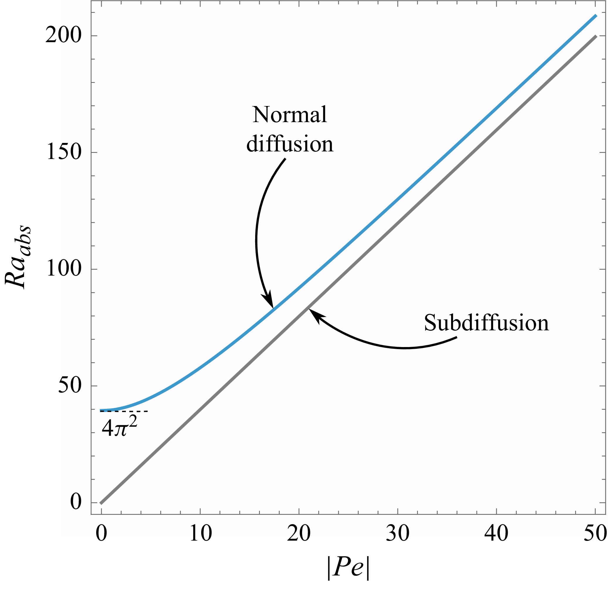
Figure 3. Transverse modes $(\phi = 0)$ with $n=1$ : comparison between the absolute instability threshold for normal diffusion (Delache et al. Reference Delache, Ouarzazi and Combarnous2007; Barletta Reference Barletta2019) and that for subdiffusion, showing up the earlier onset of absolute instability under subdiffusion. The black line corresponds to the threshold value ${\textit{Ra}}_{\textit{abs}}$ versus $|{\textit{Pe}}|$ for subdiffusion. The blue line corresponds to the threshold value ${\textit{Ra}}_{\textit{abs}}$ versus $|{\textit{Pe}}|$ for normal diffusion.

Figure 1 illustrates the results of the linear stability analysis for subdiffusion as they emerge from the arguments presented in § 5 and from the evaluation of the absolute instability threshold given by (6.8) with $n=1$ .

Figure 2 shows graphically that the so-called holomorphy requirement (Suslov Reference Suslov2006; Barletta Reference Barletta2019) is satisfied by the saddle points given by (6.7). This means that one can continuously deform the integration domain for the right-hand side of (6.3), namely the line $\textrm{Im} (k) = 0$ , into a curve crossing the saddle points through a path which is locally of steepest descent for ${ {\textrm{Re}}}(\lambda (k))$ . Such paths of steepest descent are displayed in figure 2 as red lines. The blue dots are the saddle points, while the black dot is the singularity $k = -i \pi$ . The saddle points are at the intersections of the isolines ${ {\textrm{Re}}}(\lambda (k)) = 0$ . The union of the deformed path crossing the saddle points and the original integration path, $\textrm{Im} (k) = 0$ , must yield a contour that does not contain any singularity of ${ {\textrm{Re}}}(\lambda (k))$ . Figure 2 demonstrates that the latter statement holds true or, equivalently, that the holomorphy requirement can be satisfied.

Figure 3 displays a comparison between the trends of ${\textit{Ra}}_{\textit{abs}}$ for the case of transverse modes with normal diffusion (data reported by Delache et al. (Reference Delache, Ouarzazi and Combarnous2007) and Barletta (Reference Barletta2019)) with (6.8) for subdiffusion. One can conclude that the transition to absolute instability for normal diffusion requires larger values of ${\textit{Ra}}$ than for subdiffusion, for every fixed value of ${\textit{Pe}}$ . As suggested by figure 3, for large values of ${\textit{Pe}}$ , the difference, $\Delta {\textit{Ra}}_{\textit{abs}}$ , between ${\textit{Ra}}_{\textit{abs}}$ for normal diffusion and subdiffusion tends to an asymptotic value that can be evaluated by employing Richardson’s extrapolation, namely $\Delta {\textit{Ra}}_{\textit{abs}} \approx 7.3356$ . A common feature of normal diffusion and subdiffusion displayed in figure 3 is that, with ${\textit{Pe}}=0$ , the transition to absolute instability takes place at critical conditions without any gap in ${\textit{Ra}}$ , i.e. with ${\textit{Ra}} = {\textit{Ra}}_c = 4\pi ^2$ for normal diffusion and ${\textit{Ra}} = {\textit{Ra}}_c = 0$ for subdiffusion. Table 1 shows some representative values of ${\textit{Ra}}_{\textit{abs}}$ versus $|{\textit{Pe}}|$ for subdiffusion and for normal diffusion with $n=1$ and $\phi =0$ . Such values could serve as benchmark data for future theoretical and numerical studies of this problem.

Table 1. Values of ${\textit{Ra}}_{\textit{abs}}$ versus $|{\textit{Pe}}|$ for $n=1$ and $\phi = 0$ with either subdiffusion or normal diffusion.