


Non-technical Summary
Shells of foraminifers provide indispensable data for paleoceanography, paleoecology, and paleoclimate reconstruction. This study analyzes the preservation of shell, specifically where and why bioerosion (i.e., drill holes) occur in planktonic foraminifera shells. We examined 2588 specimens from eight species and used statistical analyses and numeric models to map the distribution of these drill marks within each species. Our findings reveal that the density and location of drill holes differ between spinose and non-spinose species, with spinose species tending to have more holes. Species with thinner tests (spinose) are preferentially perforated in the earlier whorls, while those with thicker shells (non-spinose) exhibit more holes in the ultimate chambers. Foraminiferal bioeroders likely select drilling sites based on a balance between minimizing the effort required to penetrate the test and maximizing access to nutrient-rich content. In summary, our study revealed distinct bioerosion patterns across foraminiferal species, suggesting that morphological characteristics contribute to the varying vulnerability of sectors and species to bioerosion.
Introduction
Understanding of the ecological interactions involving planktonic foraminifera (marine single-celled microorganisms) has advanced but remains limited, particularly regarding their role as prey (Schiebel and Hemleben Reference Schiebel and Hemleben2017; Grigoratou et al. Reference Grigoratou, Monteiro, Schmidt, Wilson and Ward2019; Greco et al. Reference Greco, Morard and Kucera2021; Ying et al. Reference Ying, Monteiro, Wilson and Schmidt2023). These interactions often infer foraminifera as occasional prey for a vast number of taxa, and in high abundances, they serve as a crucial link in energy transfer between the phytoplankton and nekton (Lipps and Valentine Reference Lipps and Valentine1970). However, predatory activity on planktonic foraminifera is indirectly inferred by drilling traces in tests collected from plankton net samples (Harbers Reference Harbers2011; Jentzen Reference Jentzen2016; Siccha et al. Reference Siccha, Morard, Meilland, Iwasaki, Kucera and Kimoto2023). This activity is not yet fully documented (Schiebel and Hemleben Reference Schiebel and Hemleben2017). Observing these trophic interactions in situ is extremely challenging, and laboratory culturing of planktonic foraminifera has limitations in representing the entire community within its natural habitat (Hemleben et al. Reference Hemleben, Spindler and Anderson1989; Culver and Lipps Reference Culver, Lipps, Kelley, Kowalewski and Hansen2003).
Such interactions can leave bioerosional traces, defined as the process by which the removal and transport of hard substrates occur through the action of biological agents (Taylor and Wilson Reference Taylor and Wilson2003; Tribollet et al. Reference Tribollet, Radtke, Golubic, Reitner and Thiel2011). According to Boltovskoy and Wright (Reference Boltovskoy and Wright1976), bioerosion is a valuable source of paleoecological information, especially when the studied species lacks living representatives. This process can occur through mechanical means (bioabrasion: scraping or drilling), chemical removal (biocorrosion: attachment, drilling, or dissolution), or as most observed in nature, through a combination of both (Tribollet et al. Reference Tribollet, Radtke, Golubic, Reitner and Thiel2011). The number and nature of drill holes tend to reduce test resistance, leading to mechanical fragmentation and subsequent differential dissolution and eventual destruction (Douglas Reference Douglas1973). If bioerosion is selective by site, species, and/or size (e.g., Lipps Reference Lipps, Lipps, Berger, Buzas, Douglas and Ross1979), fossil assemblages may not accurately reflect the original assemblage composition (Culver and Lipps Reference Culver, Lipps, Kelley, Kowalewski and Hansen2003).
Significant advances in understanding bioerosional patterns in foraminifera, particularly those associated with benthic foraminifera, have been made (e.g., Sliter Reference Sliter1971, Reference Sliter1975; Douglas Reference Douglas1973; Arnold et al. Reference Arnold, d'Escrivan and Parker1985; Malumián et al. Reference Malumián, Cabrera, Náñez and Olivero2007; Sengupta and Nielsen Reference Sengupta and Nielsen2009). In comparison, planktonic foraminifera have not been fully explored, with few dedicated studies available (e.g., Nielsen and Nielsen Reference Nielsen and Nielsen2001; Nielsen et al. Reference Nielsen, Nielsen and Bromley2003; Frozza et al. Reference Frozza, Pivel, Suárez-Ibarra, Ritter and Coimbra2020). This study aims to address this gap, focusing on the characterization and quantification of bioerosion in late Quaternary planktonic foraminifera, with an emphasis on site-selectivity analysis of bioerosional traces. However, we do not focus on identification of bioeroders, which is typically based on size, shape of traces, and the dimensions of specimens. This approach, often employed in identifying predators (e.g., Sliter Reference Sliter1971; Arnold et al. Reference Arnold, d'Escrivan and Parker1985; Klompmaker et al. Reference Klompmaker, Kowalewski, Huntley and Finnegan2017; Karapunar et al. Reference Karapunar, Werner, Simonsen, Bade, Lücke, Rebbe, Schubert and Rojas2023), is not within the scope of the present research, which focuses on identifying the characteristics of their activity.
By analyzing samples from core SAT048A, previously studied by Frozza et al. (Reference Frozza, Pivel, Suárez-Ibarra, Ritter and Coimbra2020), who found significant correlations between bioerosion rates and paleoproductivity estimates, this study investigates the frequency and spatial distribution of bioerosional traces in planktonic foraminifera tests. We prioritize key species at our site based on their paleoecological significance and high relative abundance. These species include Globigerinita glutinata, Globigerina bulloides, Trilobatus sacculifer, Neogloboquadrina incompta, Globorotalia truncatulinoides, and Globorotalia inflata, along with the Globigerinoides clade and its subspecies. Encompassing the 43 to 5 ka time interval and constituting the first quantitative exploration of site selectivity in the bioerosion patterns of the group, our objective is to significantly contribute to its understanding in western South Atlantic assemblages.
Material and Methods
This study uses marine sediment samples extracted from core SAT048A, which was previously analyzed by Frozza et al. (Reference Frozza, Pivel, Suárez-Ibarra, Ritter and Coimbra2020) for foraminiferal assemblages and bioerosion frequencies. Core SAT048A was retrieved from the continental slope of the Pelotas Basin, in the southernmost Brazilian continental margin, western South Atlantic (29°11′52.110″S, 47°15′10.219″W; 3.54 m length; at a depth of 1542 m below sea level) (Fig. 1).
Sampling area with location of SAT048A core (white dot), the northern boundary of the Pelotas Basin (horizontal dashed black line), and bathymetry of the ocean floor (colored), including a color bar with water-depth ranges (right). The inset shows the location of the study area in South America.

All core samples were analyzed collectively, disregarding downcore variations. The samples were washed in a 63 μm aperture sieve, dried at <60°C, and sieved again for a fraction >150 μm. All specimens in a subsample of at least 300 planktonic foraminifera tests were originally picked for census counts (Patterson and Fishbein Reference Patterson and Fishbein1989). Samples from sediment core SAT048A correspond to the 43–5 ka time interval (Marine Isotope Stages 3 to 1; Frozza et al. Reference Frozza, Pivel, Suárez-Ibarra, Ritter and Coimbra2020; Suárez-Ibarra et al. Reference Suárez-Ibarra, Frozza, Palhano, Petró, Weinkauf and Pivel2022).
Bioerosion Spatial Characterization
Fifty samples were analyzed to quantify and characterize spatial and frequency patterns of bioerosional traces found on planktonic foraminifera tests. We focused on the species Globigerinita glutinata, Globigerina bulloides, Trilobatus sacculifer (including the four morphotypes T. sacculifer, T. quadrilobatus, T. immaturus, T. trilobus), Neogloboquadrina incompta, Globorotalia truncatulinoides, and Globorotalia inflata, as well as the Globigerinoides clade (Globigerinoides ruber albus and Globigerinoides ruber ruber, following Morard et al. [Reference Morard, Füllberg, Brummer, Greco, Jonkers, Wizemann and Weiner2019]). We chose these species because they represent tropical to subpolar provinces and have high relative abundances in our site (Boltovskoy et al. Reference Boltovskoy, Boltovskoy, Correa and Brandini1996; Kucera Reference Kucera, Hillaire–Marcel and de Vernal2007).
To visualize the underlying probability distribution of bioerosional traces on planktonic foraminifera tests, we used a standard sector-based approach (Kowalewski Reference Kowalewski2002), along with kernel density estimation plots and hotspot mapping as visualization tools.
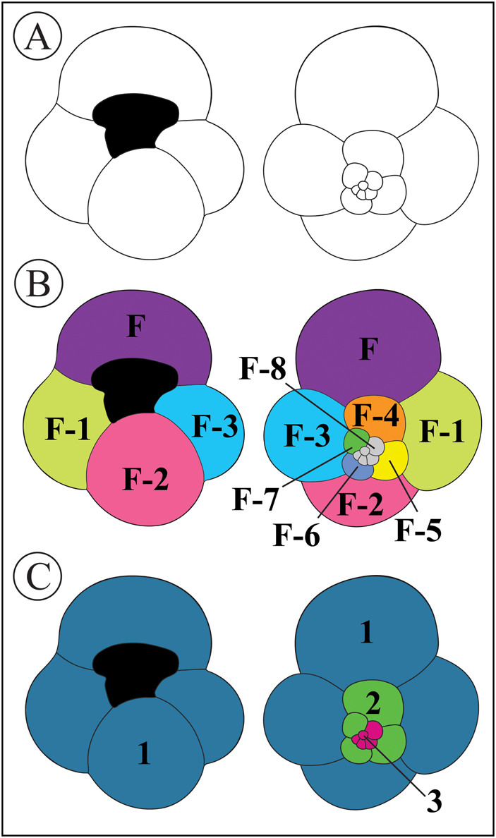
The objective was to evaluate whether structural differences in each chamber wall, caused by the ontogenetic development of planktonic foraminifers (Hemleben et al. Reference Hemleben, Spindler, Breitinger and Deuser1985), influence bioerosional patterns. To do this, we divided the specimens into umbilical/spiral views and chambers (Fig. 2B). To compare the trace frequency among species, we grouped the chambers with similar characteristics presented by their position in the different whorls of the tests. As planktonic foraminifera taxa exhibit a distinct number of chambers per whorl (Kennett and Srinivasan Reference Kennett and Srinivasan1983), the tests were categorized into three distinct chamber groups: final, penultimate, and initial whorl with proloculus, Regions 1, 2, and 3, respectively (Fig. 2C).
Schematic graphical representations of a Globigerina bulloides test. A, Delimitation of the outer- and inter-chamber lines of G. bulloides umbilical (left side) and spiral (right side) views, respectively, and main aperture. B, Arrangement of chambers in a sequence based on the coiling direction, where “F” designates “final,” “F-1” represents “penultimate,” and so on. C, Grouping of chambers with umbilical and spiral views, as described in the main text, of the last whorl (Region 1), penultimate whorl (Region 2), and initial whorls (Region 3), respectively. The color scheme was employed in the illustrations to distinguish the boundaries between chambers and regions.
To determine the bioerosional trace location on the test wall for each species, we visually transferred their positions onto a schematic graphical representation (derived from authentic specimens, one from each species, cataloged in the Mikrotax database; Huber Reference Huber, Petrizzo, Young, Falzoni, Gilardoni, Bown and Wade2017), as exemplified in Figure 2A (additional images of all species representations in .jpg format are provided in the Supplementary Material). We differentiated bioerosional traces between complete drill holes (successful drilling) and incomplete drill holes (unsuccessful drilling).
Because the whorls present different sizes—similar to the uneven-sector approach addressed by Kowalewski (Reference Kowalewski2002)—we used the polygon selection tool in FIJI (Schindelin et al. Reference Schindelin, Arganda-Carreras, Frise, Kaynig, Longair, Pietzsch and Preibisch2012) to measure the area (pixel2) of each region (whorl). We then tracked the trace positions to quantify the traces per unit area. Schematic graphical representations of all the analyzed species along with the counting and frequencies of the traces per chamber and regions are provided in Supplementary Tables 1 and 2.
To numerically transform the trace positions from the graphical representation into x and y pixel coordinates, we used FIJI software (Schindelin et al. Reference Schindelin, Arganda-Carreras, Frise, Kaynig, Longair, Pietzsch and Preibisch2012). First, the graphical representations were converted into 8-bit binary images. Subsequently, the positions of the traces were marked, and their corresponding pixel coordinates were extracted to a .csv file. Each point was labeled with specimen and trace numbers to facilitate identification and data aggregation. The identification and attributes of each specimen and trace, as well as the pixel coordinates and chamber/region identifications are provided in Supplementary Table 3.
Kernel density estimation plots were generated using OriginPro software (v. 2023b, OriginLab, Northampton, Mass.), through the input of the x and y pixel coordinates of all traces, along with complete and incomplete drill holes for each species, in both umbilical and spiral sides. The bandwidth was selected using the Silverman's rule of thumb method (Silverman Reference Silverman1986). The exact estimation for density method was chosen to iteratively calculate the density at each point by considering the contributions of nearby data points, with the bandwidths controlling the trade-off between bias and variance in the density estimate. Finally, the interpolation of the density points was made to improve the speed of analysis in a 32 x,y grid. It is important to note that the kernel density was utilized to visualize the distribution patterns and concentrations of drill holes within each species. The density values derived from this analysis were not compared across species to avoid potential biases that could arise from quantitative comparisons.
The hotspot mapping was performed through the output of the kernel density estimation in 10% of the highest density values (Nelson and Boots Reference Nelson and Boots2008), utilizing the heatmap plot function in OriginPro Software (v. 2023b, OriginLab). After the software output, the graphical representations of the species (Supplementary Material) were overlaid on the plots to construct point patterns, kernel density estimation, and hotspot mapping figures.
Hypothesis Testing
To test site selectivity on planktonic foraminifera tests, we applied two different attributes: (1) whether there are complete or incomplete drill holes and (2) wall types (spinose, non-spinose macro- and microperforate). To investigate whether bioerosional traces occur preferentially in a particular region of the test, we applied an exact test of goodness of fit for each species. This nonparametric test is suitable for datasets containing categories with fewer than five observations, which can be problematic for chi-square tests. This analysis compares the observed trace frequencies in the three predefined regions with expected frequencies based on the assumption that trace abundance is proportional to the surface area of each region. We rejected the null hypothesis of random trace distribution at a 5% significance level. The multinom_test() function from the rstatix package in R was used for this analysis (Kassambara Reference Kassambara2023). Additionally, pairwise binomial tests with Bonferroni correction were performed as a post hoc test to identify specific regions with significant differences in trace frequency using the pairwise_binom_test_against_p() function. These tests were graphically complemented with a correspondence analysis (CA).
The contingency tables used to perform this exploratory technique were built using the trace density values categorized by region and by chambers. To ensure consistency in the number of categories across species, chambers F-6 to F-10 were combined into a single class (for species with more than seven chambers). The CA function from the FactoMiner package was selected for this purpose (Lê et al. Reference Lê, Josse and Husson2008). The analyses were conducted using the R language (R Core Team 2023).
Results
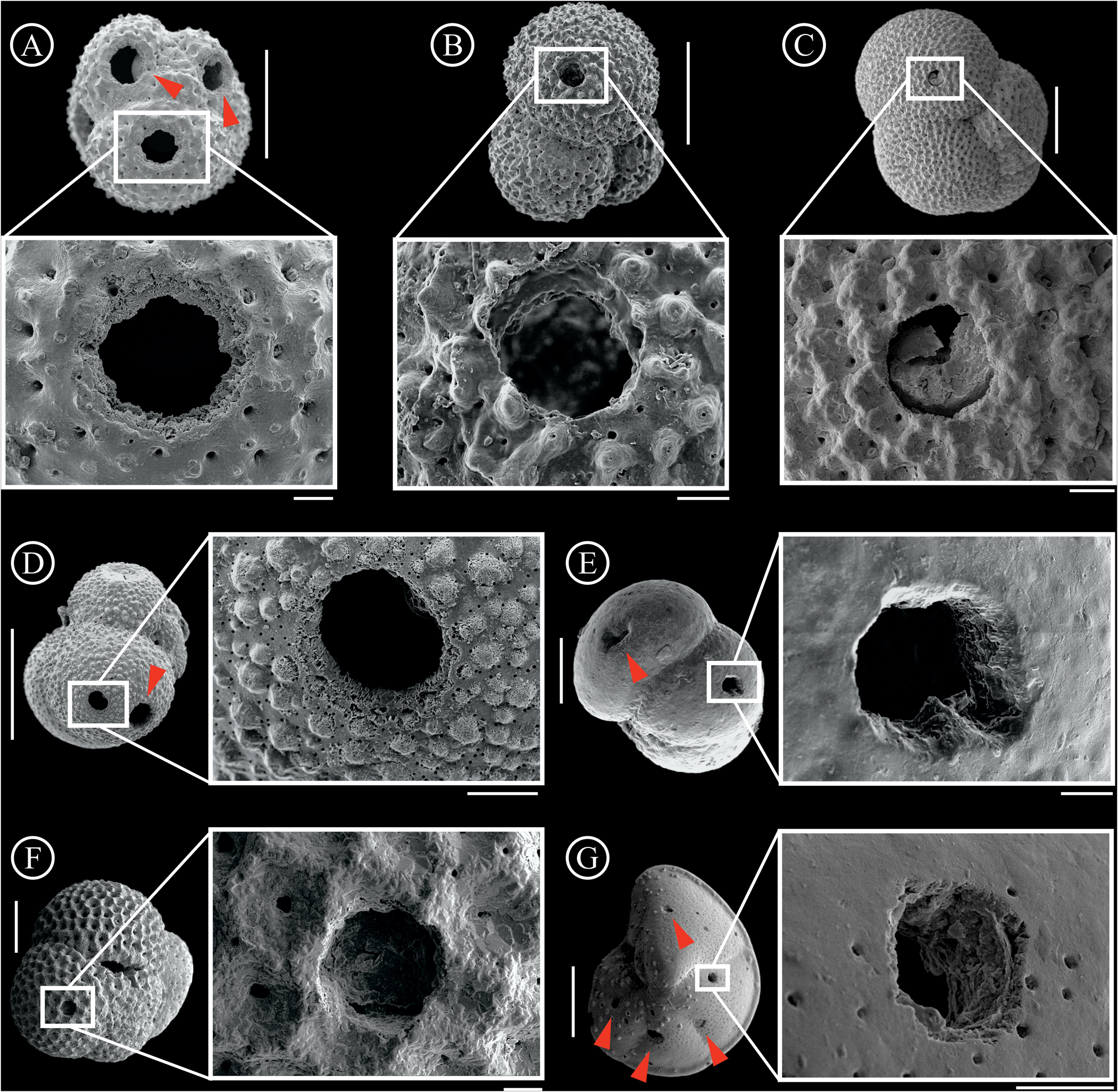
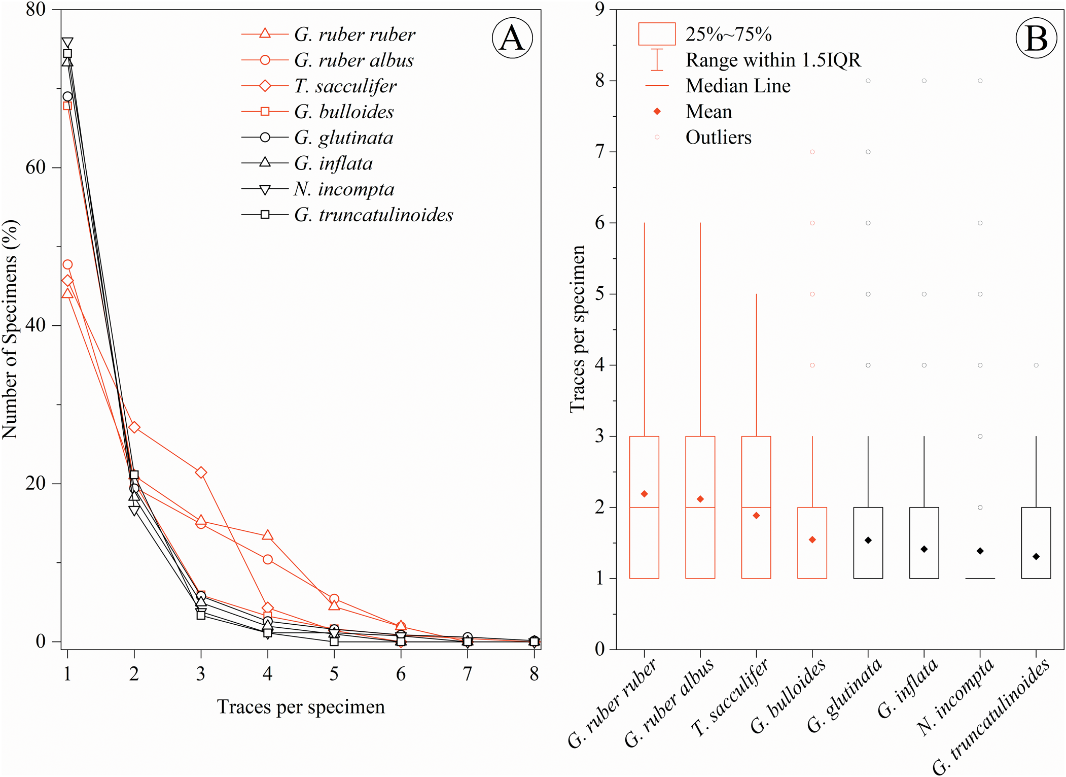
Out of all the 17,539 analyzed specimens, 2588 tests (~14.75%) were bioeroded (Table 1). Examples of the detailed traces are provided in Figure 3. From the total of 4392 traces, 3560 (81.06%) correspond to complete drill holes and 832 (18.94%) to incomplete drill holes. Within the drilled specimens, 964 (24.95%) exhibit more than one bioerosional trace per test. When species are examined individually, about half (50% to 56%) of the Globigerinoides ruber albus , Globigerinoides ruber ruber, and Trilobatus sacculifer bioeroded individuals present more than one trace per specimen. Subsequently, about one-third (32% and 31%, respectively) of the bioeroded tests of Globigerina bulloides and Globigerinita glutinata also show more than one trace. Finally, about a quarter (from 24% to 27%) of Globorotalia inflata, Globorotalia truncatulinoides, and Neogloboquadrina incompta tests present more than one trace per specimen (Fig. 4A). The distribution of the traces among the populations can be seen in the box plots (Fig. 4B) evidencing the ranging, means, and outliers of each species.
Data of the eight analyzed taxa with the number of specimens in all samples and the specimens with traces, as well as the number of traces per species and discriminated by holes and pits.

Planktonic foraminifera tests presenting bioerosional traces and traces in detail. A, Globigerinoides ruber albus and complete drill hole in detail, B, Globigerina bulloides and complete drill hole in detail, C, Neogloboquadrina incompta and incomplete drill hole in detail, D, Globigerinita glutinata and complete drill hole in detail, E, Globorotalia inflata and complete drill hole in detail, F, Trilobatus sacculifer and incomplete drill hole in detail, G, Globorotalia truncatulinoides and complete drill hole in detail. Scale bars: vertical bars for tests = 100 μm; horizontal bars for details = 10 μm. Red arrows indicate other traces on the tests.
Number of traces per specimen and bioeroded specimen. Quantity of traces per specimen related to the number of bioeroded specimens (A) and box plots of the distribution of the specimens in the number of traces per specimen (B). Distinct colors correspond to spinose (red) and non-spinose (black) species. In-plot legends for line types and box-plot characteristics.
Moreover, all the bioerosional trace frequencies in the analyzed planktonic foraminifera species decrease toward juvenile chambers (Fig. 5A), as expected given the decreasing size of the chambers. However, the precise nature of this relationship still warrants further investigation. For G. ruber albus, G. ruber ruber, and T. sacculifer, between 10% and 20% of the bioerosional traces occur in the final chamber (F, Fig. 2B), increasing to 20–30% for the penultimate (F-1, Fig. 2B) and antepenultimate (F-2, Fig. 2B) chambers. Although G. bulloides shows a similar trace frequency, the relative abundances for the F and F-1 chambers (Fig. 2B) are higher (between 20% and 35%). On the other hand, while G. inflata displays similar trace frequencies for the F and F-1 chambers (Fig. 2B) (around 30–35%), between 30% and 40% of the traces occur within the final chamber for the species G. glutinata, N. incompta, and G. truncatulinoides (Supplementary Table 1).
Trace frequency vs. chamber identification (A) and for regional identification (B). Distinct colors correspond to spinose (red) and non-spinose (black) species. In-plot legends for line types.

In the final whorl, trace frequencies per region (Fig. 5B) indicate that about 96% of incomplete and 90% of complete drill holes occur in non-spinose species, while about 69% of incomplete and 80% of complete drill holes occur in spinose species (Fig. 5B, Region 1). The distinction between spinose and non-spinose species becomes apparent in the penultimate whorl (Fig. 5B, Region 2), as well as in the occurrence of incomplete and complete drill holes. In this region, non-spinose specimens exhibited lower values, approximately 3% for incomplete and 9% for complete drill holes, while spinose specimens demonstrated higher values, around 19% for incomplete and 28% for complete drill holes. The initial whorls (Fig. 5B, Region 3) present similar frequencies among the groups, ranging from approximately 0.3% to about 1.6% (Supplementary Table 2).
The analysis of bioerosional patterns reveals consistent groupings between spinose and non-spinose species, as seen in the number of traces per specimen (Fig. 4A) and the frequency of the trace distribution per chamber (Fig. 5A). CA of trace frequencies normalized by surface area strengthens the evidence for distinct bioerosional patterns among foraminiferal species. This is illustrated by the separation of ellipses representing spinose and non-spinose groups in the CA biplot (Fig. 6).
Correspondence analysis (CA) results performed on contingency tables. (A) Biplot illustrating associations between eight species and the number of traces per specimen. (B) Biplot showcasing associations between eight species and three test regions based on their trace density distribution. (C) Biplot depicting associations between eight species and seven chambers based on their trace density distribution.

Analysis of the number of traces per test for each species (Fig. 6A) revealed that spinose species are generally associated with two or more traces, except for G. bulloides. In contrast, non-spinose species tend to be associated with a single trace. In the analysis by region (Fig. 6B), spinose species cluster closer to Region 2 (penultimate whorl), indicating a higher density of traces in this sector, while non-spinose species associate more with Region 1 (final whorl). These observations suggest contrasting bioerosional patterns between these groups, with different patterns in G. inflata, the only species associated with Region 3 (first whorls). The pattern of association observed in Figure 6B is repeated, in general terms, when traces are analyzed by chambers (Fig. 6C). Again, non-spinose species tend to be associated with the final chambers (F to F-2). However, at this finer resolution, even species within the same group exhibit higher trace densities in different chambers.
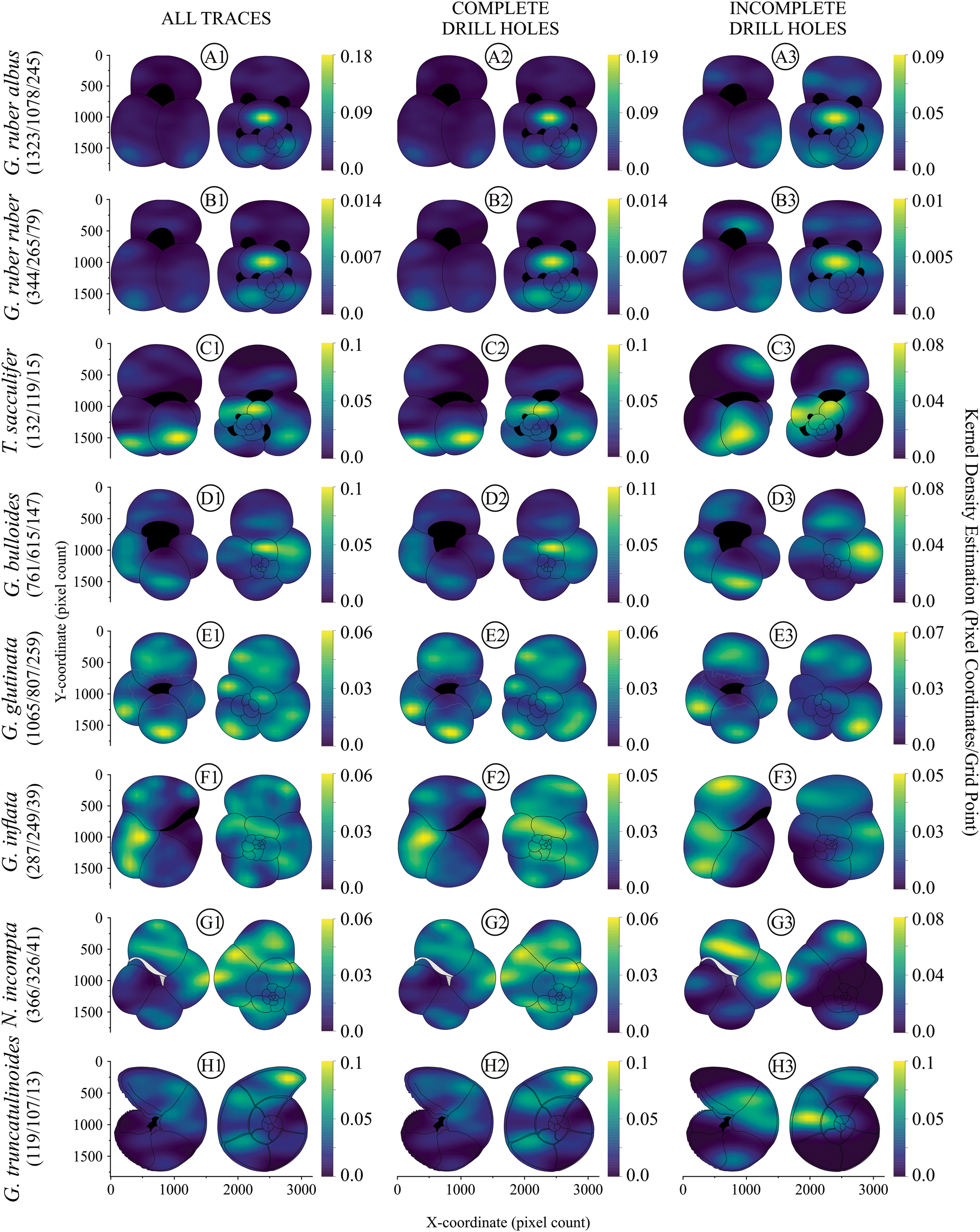
Regarding the kernel density estimation, originated from the traces distribution (Fig. 7), the spinose species G. ruber albus, G. ruber ruber, T. sacculifer, and G. bulloides presented high trace density values in the chambers of the penultimate whorl (Fig. 8A1–D1). The final chamber (F; Fig. 2C) showed lower trace densities in globigerinid species (Fig. 8A1–D1), whereas G. glutinata, G. inflata, G. truncatulinoides, and N. incompta (Fig. 8E1–H1), displayed moderate to high trace densities in the same chamber. Among these species, G. glutinata (Fig. 8E1) exhibited the pattern with greatest spread in the densities of the traces, featuring exclusively moderate densities without any high concentrations, compared with the other species, particularly in certain chambers and/or regions. In contrast, G. inflata and G. truncatulinoides (Fig. 8F1,H1) showcased their highest densities in the F and F-1 chambers, which can be observed in the hotspots (Fig. 9F1,H1), while N. incompta (Fig. 8G1) demonstrated moderate density in both, and in the penultimate whorl.
Distribution of the traces (black dots) on the planktonic foraminifera tests. A, Globigerinoides ruber albus, B, Globigerinoides ruber ruber, C, Trilobatus sacculifer, D, Globigerina bulloides, E, Globigerinita glutinata, F, Globorotalia inflata, G, Neogloboquadrina incompta, and H, Globorotalia truncatulinoides. Each taxon is presented in both umbilical and spiral views and organized in three columns, with: all traces (1), complete drill holes (2), and incomplete drill holes (3). The number of bioerosional traces is presented in parentheses with each species’ name as all traces/complete drill holes/incomplete drill holes. The x and y axes correspond to the x and y coordinates of the pixel counts at bioerosional trace locations.

Kernel density estimation of the analyzed species: A, Globigerinoides ruber albus, B, Globigerinoides ruber ruber, C, Trilobatus sacculifer, D, Globigerina bulloides, E, Globigerinita glutinata, F, Globorotalia inflata, G, Neogloboquadrina incompta, and H, Globorotalia truncatulinoides. Each taxon is presented in both umbilical and spiral views and organized in three columns with: all traces (1), complete drill holes (2), and incomplete drill holes (3). The number of bioerosional traces is presented in parentheses with each species’ name as all traces/complete drill holes/incomplete drill holes. The x and y axes correspond to the x and y coordinates of the pixel counts at bioerosional trace locations. The color scheme represents the kernel density estimation, showcasing the concentration of pixel coordinates/bioerosional traces per grid point in the graphical representation. The right-side scale transitions from dark blue to yellow, indicating points of lower to higher densities. The densities were adjusted in x × 106 to facilitate visualization.
Hotspot mapping based on the 10% highest kernel density estimation values of the analyzed species: A, Globigerinoides ruber albus, B, Globigerinoides ruber ruber, C, Trilobatus sacculifer, D, Globigerina bulloides, E, Globigerinita glutinata, F, Globorotalia inflata, G, Neogloboquadrina incompta, and H, Globorotalia truncatulinoides. Each taxon is presented in both umbilical and spiral views and organized in three columns with: all traces (1), complete drill holes (2), and incomplete drill holes (3). The number of bioerosional traces is presented in parentheses with each species’ name as all traces/complete drill holes/incomplete drill holes. The x and y axes correspond to the x and y coordinates of the pixel counts at bioerosional trace locations.

To test the hypothesis of site-selective bioerosion on planktonic foraminifera species, a multinomial exact test of goodness of fit was employed. The expected frequency of traces was calculated assuming two conditions: (1) a random trace distribution across the foraminifera test, and (2) proportion of trace abundance to the estimated surface area of three regions of the tests defined based on whorl position (Fig. 2C, Supplementary Table 2). The observed frequencies of traces deviated significantly from expected values in some species (p < 0.001). Spinose species, including G. ruber albus, G. ruber ruber, T. sacculifer, and G. bulloides, exhibited lower trace frequencies in Region 1 (last whorl) compared with expected values, and higher frequencies in Region 2 (penultimate whorl) (Supplementary Table 4, Supplementary Fig. S1). This suggests a nonrandom distribution of bioerosion with a preference for chambers located in the penultimate whorl. In contrast, non-spinose species like G. glutinata, G. truncatulinoides, and N. incompta displayed no significant differences in trace frequency across regions, indicating a more random pattern of bioerosion. Notably, G. inflata (non-spinose) behaved similarly to the spinose group, with a preference for the penultimate whorl.
Given the high proportion of complete drill holes compared with incomplete ones, the densities of complete drill holes displayed almost the same pattern as the total traces (Fig. 8A2–H2). Comparing incomplete drill holes reveals that, in contrast to both total traces and complete drill holes, tests of the analyzed species exhibit distinct patterns (Fig. 8C3–H3) and/or variations in the densities of the same chamber/region (Fig. 8A3,B3). Notably, some species displayed specimens with significantly fewer incomplete drill holes than others, mainly T. sacculifer and G. truncatulinoides (Fig. 8C3,H3).
Within the initial whorl region, complete drill-hole densities were high in all spinose species, whereas incomplete drill holes exhibited moderate to low densities across all non-spinose species (Figs. 8E3–H3, 9A2–D2,), showing no hotspot points (Fig. 9E3–H3). Globigerinita glutinata exhibited notably high incomplete drill-hole densities, particularly in chamber F-1 (Figs. 8E3, 9E3), unlike the moderate density of complete drill holes observed in all tests (Fig. 8E2),
Discussion
Assessment of bioerosion in planktonic foraminifera is currently undergoing a phase of progressive development. Detailed examinations of bioerosion within assemblages, focusing on trace characteristics such as shape, size, and ichnology, has only been limited to the works of Nielsen and Nielsen (Reference Nielsen and Nielsen2001) and Nielsen et al. (Reference Nielsen, Nielsen and Bromley2003). Beyond these, only Frozza et al. (Reference Frozza, Pivel, Suárez-Ibarra, Ritter and Coimbra2020) have characterized bioerosion frequencies in planktonic foraminifera. In this study, we employ novel methods to explore previously unknown patterns of bioerosional traces in Quaternary planktonic foraminifera and provide new insights into the strategies of their bioeroders.
On the Method
In this study, we present for the first time in the literature kernel density estimation, sector-based, and hotspot mapping to characterize bioerosional patterns in planktonic foraminifera. These methods have been improved with other taxa, for instance Rojas et al. (Reference Rojas, Dietl, Kowalewski, Portell, Hendy and Blackburn2020), that spatially quantified and characterized drill holes in mollusks, introducing an approach from geometric morphometrics involving images and (semi)landmarks for trace analysis. This approach aims to avoid the accuracy loss in the spatial positioning of drill holes within oversimplified systems, such as arbitrary grids used to divide invertebrate shells into sectors. However, due to the complex 3D arrangement of the spherical and globular chambers of most planktonic foraminifera (Kennett and Srinivasan Reference Kennett and Srinivasan1983), it proves challenging to photographically capture sharp edges and visualize the drill holes to apply the landmark analyses. Yet, according to Nielsen and Nielsen (Reference Nielsen and Nielsen2001), such traces tend to be much smaller compared with those found in other bioeroded taxa (e.g., ostracods, bivalves, gastropods).
Kernel density estimation and hotspot mapping have inherent limitations, particularly when applied without the spatial accuracy of landmarking techniques. For the Silverman's rule of thumb method, a fixed-bandwidth approach, the use of a single, consistent bandwidth across the entire dataset, led to some maps appearing oversmoothed (e.g., Fig. 8E2,F2). This oversmoothing could obscure finer details, particularly in regions where the data might have multiple peaks, making the identification of the number of peaks somewhat speculative. However, the method still successfully highlights the primary areas of interest on the tests and produces very little visual difference from the normal reference bandwidth (Sheather Reference Sheather2004). Despite these challenges, these visualization tools are valuable, because they provide an informative overview of the spatial distribution patterns and are relatively easy to apply, making them practical for use in similar studies.
Another important consideration is that the sector-based approach is limited by the choice of spatial scale for the test regions. This selection can influence the confidence in interpreting the preferred chambers targeted by bioeroders. While this choice may affect our assumptions, the sector-based approach remains a robust tool for confirming the general patterns observed in the other analyses.
Inferences on Bioerosional Patterns
The diverse results presented here enable us to underscore several inferences about the bioerosional patterns observed in planktonic foraminifera tests of core SAT-048A: (1) The number of traces per specimen is remarkable high. (2) The frequency of specimens per quantity of traces in the tests reveals distinct groups, specifically between spinose and non-spinose species, with some variations. (3) The trace distribution exhibits high frequency in the final chambers, greatly decreasing toward the early chambers, as expected following the decreasing chamber size. When specific regions are examined, spinose and non-spinose species show similar trends, although with differences in their respective ranges. (4) The density of traces is high and significatively nonrandom in chambers of the penultimate whorl for all spinose tests. (5) Non-spinose tests exhibit various patterns of densities and a more random pattern of bioerosion, ranging from a lack of site selectivity to a contrasting site selectivity, not for the group but in specific species.
On the Number of Traces per Specimen
We compare our results to those existing on benthic foraminifera due to the lack of quantitative analysis of bioerosional traces in planktonic foraminifera. Our study identifies around twice the number of bioerosional traces compared with the number of drilled specimens (Table 1), with up to eight traces observed for a single specimen (Fig. 4B). Nonetheless, in contrast to benthic foraminifera, which can exhibit up to 15 drill holes per specimen (e.g., Sliter Reference Sliter1975; Arnold et al. Reference Arnold, d'Escrivan and Parker1985), planktonic species show lower quantities (e.g., Nielsen and Nielsen Reference Nielsen and Nielsen2001; Nielsen et al. Reference Nielsen, Nielsen and Bromley2003). On the other hand, both benthic and planktonic foraminifers exhibit higher rates of multiple drilled specimens than those observed across predation in taxa such as bivalves (e.g., Anderson Reference Anderson1992; Karapunar et al. Reference Karapunar, Werner, Simonsen, Bade, Lücke, Rebbe, Schubert and Rojas2023) and ostracods (e.g., Ruiz et al. Reference Ruiz, Abad, González-Regalado, Tosquella, García, Toscano, Muñoz and Pendón2011; Villegas-Martín et al. Reference Villegas-Martín, Ceolin, Fauth and Klompmaker2019).
According to Kowalewski (Reference Kowalewski2002), multiple drill holes usually suggest a parasitic action rather than predation, resembling the feeding behavior of parasites that seek their food without killing the host. However, although parasitic relations in planktonic foraminifera are not yet well understood, the record includes dinoflagellates, sporozoans, and potentially bacteria (Schiebel and Hemleben Reference Schiebel and Hemleben2017), all of which would be too small to produce the observed traces. Alternatively, parasites could be targeting the calcium carbonate from the tests instead of the cytoplasm, or the traces may be related to predation. In such a case, the elevated frequencies observed in both benthic and planktonic foraminifers could be attributed to the multichambered nature of their tests. This adaptation serves as a response to recurrent attacks aimed at accessing the content of each chamber, potentially resulting in the presence of multiple drillings (Sliter Reference Sliter1971; Arnold et al. Reference Arnold, d'Escrivan and Parker1985; Langer et al. Reference Langer, Lipps and Moreno1995; Malumián et al. Reference Malumián, Cabrera, Náñez and Olivero2007). Furthermore, the cytoplasm remains in constant motion (Schiebel and Hemleben Reference Schiebel and Hemleben2017). When the bioeroder attempts to drill one chamber, the cytoplasm can retract to the early chambers (e.g., Myers [Reference Myers1943] in benthic foraminifers), compelling them to continue drilling the chambers until they are emptied and the foraminifer is killed.
On the Frequency of Specimens per Quantity of Traces
Considering the number of bioerosional traces per drilled specimen (Fig. 4), the spinose species (i.e., Globigerinoides ruber ruber, Globigerinoides ruber albus, Trilobatus sacculifer, and Globigerina bulloides) exhibit lower values of the proportion of specimens with only one bioerosional trace. However, the frequency of specimens with more than one and even multiple traces is higher for spinose than the non-spinose species (Globigerinita glutinata, Globorotalia inflata, Neogloboquadrina incompta, and Globorotalia truncatulinoides; Fig. 4). Both groups are distinct in relation to such frequencies (Fig. 6A), which may reveal the role of spinosity in the presence of multiple drilled specimens in the assemblages.
These results raise the question of the role of spines in protecting the tests from bioeroders. The function of spines in planktonic foraminifera has been linked to enhanced efficiency in encountering and consuming larger prey (Anderson et al. Reference Anderson, Spindler, Bé and Hemleben1979; Gaskell et al. Reference Gaskell, Ohman and Hull2019). Furthermore, the spines increase the outer surface by supporting the rhizopodial network, thereby enhancing the control of buoyancy and providing support for the symbionts (Hemleben et al. Reference Hemleben, Spindler and Anderson1989; Takagi et al. Reference Takagi, Kimoto, Fujiki, Saito, Schmidt, Kucera and Moriya2019; Pearson et al. Reference Pearson, John, Wade, D'haenens and Lear2022). Although the protective function of spines against predation is well established in marine organisms (Harvell Reference Harvell1990; Klompmaker et al. Reference Klompmaker, Kelley, Chattopadhyay, Clements, Huntley and Kowalewski2019), this defensive attribute has not yet been clearly shown to protect planktonic foraminifera from predation (Grigoratou et al. Reference Grigoratou, Monteiro, Ridgwell and Schmidt2021; Ying et al. Reference Ying, Monteiro, Wilson and Schmidt2023). In any case, the spines that can appear in juvenile ontogenetic stages are few and thin, becoming numerous and thick only in adult stages (Caromel et al. Reference Caromel, Schmidt, Fletcher and Rayfield2015), and in the final stage during the gametogenesis, they are resorbed and discarded in a process that takes only a few hours (Schiebel and Hemleben Reference Schiebel and Hemleben2017).
Within the spinose group, all species but G. bulloides are associated with a high number of traces per drilled specimen (Fig. 6A). Along with the subspecies G. ruber ruber and G. ruber albus, T. sacculifer also shows similar patterns. Regarding the non-spinose species (i.e., G. glutinata, G. inflata, N. incompta, and G. truncatulinoides), all but N. incompta exhibit similarly low values of traces per specimen (Fig. 4B). The more these groups share similar morphological characteristics and well-defined ecological functions (Schiebel and Hemleben Reference Schiebel and Hemleben2017), the more this similarity influences the bioerosional patterns in the affected organisms, whether in terms of morphology (with similar microstructure and physical durability of skeletons), ecological traits, or both (Kowalewski Reference Kowalewski2002).
On the Frequency of Trace Distribution
As noted in “On the Frequency of Specimens per Quantity of Traces,” when the trace distribution in the test is analyzed, different patterns for spinose and non-spinose species arise (Fig. 6), with intermediate frequencies for G. bulloides and G. glutinata (Fig 5).
Despite the morphological variability among the species, the early whorls (initial and penultimate) tend to be much smaller than the final whorl in adult specimens, as the last chambers exponentially increase their volume with ontogenetic growth (Hemleben et al. Reference Hemleben, Spindler, Breitinger and Deuser1985; Schmidt et al. Reference Schmidt, Rayfield, Cocking and Marone2013; Caromel et al. Reference Caromel, Schmidt, Fletcher and Rayfield2015). For instance, in our graphical representation (Supplementary Table 2), the penultimate whorl makes up 14.2% of the total test area for G. ruber albus and G. ruber ruber, 8.3% for T. sacculifer, and 5.7% for G. bulloides. However, these species exhibit trace frequencies in this region, compared with the first and last whorls, of 33%, 36%, 22%, and 11.7%, respectively. This is a clear indicator that the bioerosional pattern identified in these species is not random (Supplementary Table 4, Supplementary Fig. S1). Otherwise, the frequency of traces in each region would be proportional to the exposed surface.
On Site Selectivity in Spinose Species
The identification of the preferred targets for consumers of foraminifera is often deduced by assessing the damage incurred on the tests (Culver and Lipps Reference Culver, Lipps, Kelley, Kowalewski and Hansen2003). Within spinose species, the focus of bioeroding organisms appears to be the early chambers, specifically from the penultimate whorl, as illustrated in the kernel densities (Fig. 8A1–D1) and hotspot maps (Fig. 9A1–D1), and confirmed by the multinomial exact test of goodness of fit (Supplementary Table 4, Supplementary Fig. S1). The reason for such site selectivity can be deduced by evaluating the content within the targeted chamber(s) or, if bioeroders seek calcium carbonate, by considering the variation in test thickness across different regions. Hickman and Lipps (1977) argue that when organisms consume foraminifera for calcium carbonate, they ingest the entire test, resulting in severe damage or corrosion from stomach acids. This suggests that the organisms are not creating holes but fully consuming the tests. If predators ingest foraminifera nonselectively, this damage may be collateral rather than a deliberate search for carbonate.
In this study, where both complete and incomplete drill holes are quantified, it is reasonable to presume that these traces are crafted by consumers in their pursuit of the organic content within foraminiferal chambers, as observed by Nielsen et al. (Reference Nielsen, Nielsen and Bromley2003). Nevertheless, the primary focus for bioeroders in spinose species, documented in this study by the kernel density estimation (Fig. 8A1–D1), hotspot maps (Fig. 8A1–D1) and multinomial exact test of goodness of fit (Supplementary Table 4, Supplementary Fig. S1), is one of the thickest wall regions in the tests—specifically for the chambers of the penultimate whorl. Due to ontogenetic chamber development, the early chambers tend to experience wall thickening (Erez Reference Erez2003). As each new chamber is added, a new calcite layer precipitates over all former chambers. Consequently, as the test grows, the external walls of chambers in the first and subsequent whorls become thicker (Hemleben et al. Reference Hemleben, Spindler, Breitinger and Deuser1985; Oelschläger Reference Oelschläger1989; Ofstad et al. Reference Ofstad, Zamelczyk, Kimoto, Chierici, Fransson and Rasmussen2021).
The chamber's content must provide advantages for a thicker region to become the target (e.g., Thomas and Day Reference Thomas and Day1995). In planktonic foraminifera, this advantage could come primarily from the cytoplasm, which serves as the main biomass component in planktonic foraminifera (Michaels et al. Reference Michaels, Caron, Swanberg, Howse and Michaels1995; Schiebel and Movellan Reference Schiebel and Movellan2012; Freitas et al. Reference Freitas, Bacalhau and Disaró2021). Notably, although the cytoplasm is zoned, it is predominantly situated within the inner chambers where the nucleus is securely shielded (Schiebel and Hemleben Reference Schiebel and Hemleben2017).
Within the cytoplasm of planktonic foraminifera, lipids constitute a significant component, potentially serving as an energy source for bioeroders. Planktonic foraminifera store lipid droplets densely concentrated in the innermost chambers, near the central cytoplasm, with a decreased concentration toward the periphery near the wall (Schiebel and Hemleben Reference Schiebel and Hemleben2017), making it a readily accessible and valuable resource.
Spinose species exhibit high densities of complete drill holes in their early chambers (Figs. 8A2–D2, 9A2–D2), but this distinction is not observed with incomplete drill holes (Figs. 8A3–D3, 9A3–D3), particularly in the case of G. bulloides (Fig. 9D2,D3). This is another result that reinforces the site selectivity of early chambers in spinose species based on the contrasting pattern between complete and incomplete drill holes. The substantial success-to-failure ratio in this area suggests enhanced bioerosion efficiency, which happens in locations preferred by the bioeroder (Dietl Reference Dietl2000).
Alternatively, when focusing on the ultimate whorl, particularly the final chamber, this area reveals a low-density pattern of traces in spinose species (Figs. 8A1–D1, 9A1–D1). Despite the final chambers being typically thinner than the others (e.g., Schmidt et al. Reference Schmidt, Elliott and Kasemann2008; Fehrenbacher and Martin Reference Fehrenbacher and Martin2014; Iwasaki et al. Reference Iwasaki, Kimoto, Okazaki and Ikehara2019), making them potentially more accessible for test drilling (Sliter Reference Sliter1971), the lower trace densities may be linked to frequent occurrences of incompletely filled cytoplasm in the final chamber (Michaels et al. Reference Michaels, Caron, Swanberg, Howse and Michaels1995; Schiebel and Hemleben Reference Schiebel and Hemleben2017). This reduced cytoplasmic volume in these chambers, potentially caused by nutritional deficiencies or health issues, could lead to an increase of empty chambers (Kimoto Reference Kimoto, Ohtsuka, Suzaki, Horiguchi, Suzuki and Not2015).
If the chamber's content is the main target for the drilling bioeroder, it raises a relevant discussion about where the bioerosion in planktonic foraminifera occurs. As discussed by Frozza et al. (Reference Frozza, Pivel, Suárez-Ibarra, Ritter and Coimbra2020), planktonic foraminifera can be targeted by predators and/or parasites in the water column when alive or even after the death while sedimented on the ocean floor. Throughout gametogenesis, a significant cellular reorganization occurs, and the extensive release of gametes consumes the cytoplasm, leaving the foraminiferal test empty (Caron et al. Reference Caron, Anderson, Lindsey, Faber and Lin Lim1990). In this way, the settling community predominantly consists of empty tests from individuals who reproduced and who died before reproducing (Hemleben et al. Reference Hemleben, Spindler and Anderson1989; Siccha et al. Reference Siccha, Schiebel, Schmidt and Howa2012). Hence, as benthic bioeroders find empty tests less attractive (Chester Reference Chester1993; Langer et al. Reference Langer, Lipps and Moreno1995), and the target for bioeroders here appears to be the valuable content, bioerosion through drilling is expected to occur primarily in the water column.
However, tests filled with dead cytoplasm have been found in the sediment (e.g., Hemleben and Auras Reference Hemleben and Auras1986; Davis et al. Reference Davis, Wishner, Renema and Hull2021), as well as living individuals that lost buoyancy and, being filled, settled before the individual died (Schiebel and Hemleben Reference Schiebel and Hemleben2017). Following this, it is reasonable to assume that bioerosion by drilling in planktonic foraminifera can take place either in the sediments or in the water column, with the tests whose chambers are still filled with content potentially being found in both locations.
On Site Selectivity in Non-spinose Species
Globigerinid (spinose) and globorotalid (non-spinose) species share a commonality in their macroperforate test morphology (Cifelli Reference Cifelli1982). Porosity plays a crucial role in diminishing the thickness of the test wall due to an increased surface area (Ofstad et al. Reference Ofstad, Zamelczyk, Kimoto, Chierici, Fransson and Rasmussen2021; Zarkogiannis et al. Reference Zarkogiannis, Iwasaki, Rae, Schmidt, Mortyn, Kontakiotis, Hertzberg and Rickaby2022). However, globorotalid species exhibit porous tests in early ontogenetic stages, and the porosity decreases with advancing test growth and calcification (Hemleben et al. Reference Hemleben, Spindler, Breitinger and Deuser1985). Consequently, the walls of these species become thicker in neanic to adult stages in part due to the low porosity. Additionally, some species undergo the deposition of a calcite crust while sinking in the water column (Hemleben et al. Reference Hemleben, Spindler and Anderson1989), and the thickness of this crust may potentially reach half of the total thickness of the chamber wall (Steinhardt et al. Reference Steinhardt, de Nooijer, Brummer and Reichart2015). In this way, globorotalid species can develop walls twice as thick as usual, particularly in early chambers.
The distribution of trace densities on globigerinids and globorotalids also differs. While globigerinid species show significantly high densities of traces in the early chambers (Supplementary Fig. S1), globorotalids exhibit a more random (Supplementary Fig. S1) and opposite pattern: few marks in the early, thick chambers and a moderate to high concentration in later, thinner chambers (Figs. 8F1–H1, 9F1–H1). The thicker walls of globorotalid chambers imply a significant obstacle for bioeroders. If shell thickness corresponds to shell strength and thicker shells are more difficult and time-consuming to drill (Klompmaker et al. Reference Klompmaker, Kelley, Chattopadhyay, Clements, Huntley and Kowalewski2019), then the energy expended to perforate this region is higher (e.g., Malumián et al. Reference Malumián, Cabrera, Náñez and Olivero2007).
Moreover, the only species that presents a high trace density in the final chamber is G. truncatulinoides (Figs. 8H1, 9H1). This distribution, which is more associated with the final chamber, is also observed in Figure 6C. This species is known to have a significant thickness of calcite crusts on the test wall (Zarkogiannis et al. Reference Zarkogiannis, Iwasaki, Rae, Schmidt, Mortyn, Kontakiotis, Hertzberg and Rickaby2022). However, such a crust layer tends to reduce its thickness from the oldest to the youngest chamber of the last whorl (Takayanagi et al. Reference Takayanagi, Niitsuma and Sakai1968; Hemleben et al. Reference Hemleben, Spindler, Breitinger and Deuser1985), as seen in other globorotalids as well (Steinhardt et al. Reference Steinhardt, de Nooijer, Brummer and Reichart2015). Consequently, the primary focus of bioeroders in G. truncatulinoides may be associated with the optimal location where test penetration is facilitated, given that the early chambers, where the content may be richest, are also considerably thicker and much more energy demanding.
Unlike globorotalids, G. glutinata exhibits high densities of traces and complete drill holes in several chambers of the ultimate whorl (Fig. 9E1,E2), revealing a transitional pattern that falls between site selectivity in the early chambers observed in spinose species and the final chamber for G. truncatulinoides. Globigerinita glutinata possesses a wall distinct from both globorotalids and globigerinids; it is of the microperforate type (Hemleben et al. Reference Hemleben, Spindler and Anderson1989). Microperforate species feature extremely small, evenly distributed pores across their entire chamber surface (Schiebel and Hemleben Reference Schiebel and Hemleben2017).
While it is assumed that large and numerous pores increase surface area, reducing wall thickness, small pores are thought to act in the opposite way by increasing wall resistance (Ofstad et al. Reference Ofstad, Zamelczyk, Kimoto, Chierici, Fransson and Rasmussen2021; Zarkogiannis et al. Reference Zarkogiannis, Iwasaki, Rae, Schmidt, Mortyn, Kontakiotis, Hertzberg and Rickaby2022). However, it is assumed that the G. glutinata wall is neither as thick as that of globorotalids nor overly easy to perforate like globigerinids. This suggests that this species may not exhibit clear site selectivity but rather a slight preference for the penultimate whorl, where a higher density of complete drill holes rather than incomplete drill holes is observed (Fig. 8E2,E3).
Where It's Worth It
The lower point dispersion among non-spinose species in the groupings shown by the CA (Fig. 6A) may reflect the influence of these species’ test walls on modulating the number of traces per specimens. As discussed, the walls of non-spinose species can be thicker than those of spinose species, which can lead the bioeroders to avoid expending energy drilling multiple times in pursuit of the chambers’ contents, as also observed by Malumián et al. (Reference Malumián, Cabrera, Náñez and Olivero2007).
This pattern, coupled with the distinct site selectivity observed in spinose (Figs. 8A1–D1, 9A1-D1, Supplementary Fig. S1) and in some non-spinose species (Figs. 8G1,H1, 9G1,H1, Supplementary Fig. S1), reveals a strategic approach by bioeroders. They may prioritize thinner, easier-to-penetrate regions if locations with high caloric value content are in thicker, harder-to-drill sections of the tests. Such highly localized traces for each group of wall type possibly represent a uniform record of a single behavior (Kowalewski Reference Kowalewski2002). These observations support established cost–benefit models wherein bioeroders balance the energy spent on drilling with the potential reward of accessing the nutrient-rich content (Klompmaker et al. Reference Klompmaker, Kelley, Chattopadhyay, Clements, Huntley and Kowalewski2019 and references therein).
It is essential to point out that throughout ontogeny, the characteristics of foraminiferal test walls do not remain constant. Instead, they can undergo diverse changes, including the lamellar deposition of calcite; the development of pores, pustules, and spines; the shedding of spines; the deposition of gametogenic calcite after reproduction; and the formation of a calcite crust (Takayanagi et al. Reference Takayanagi, Niitsuma and Sakai1968; Hemleben Reference Hemleben1975; Caromel et al. Reference Caromel, Schmidt, Fletcher and Rayfield2015). In fact, even spinose species that have porous walls may exhibit a non-spinose appearance in the sediment due to the precipitation of a thin veneer resulting from gametogenic calcite (Steinhardt et al. Reference Steinhardt, de Nooijer, Brummer and Reichart2015). To mitigate such issues, we specifically chose the size fraction that is believed to represent most of the assemblage that has already reached the adult stages (Brummer et al. Reference Brummer, Hemleben and Spindler1987; Peeters et al. Reference Peeters, Ivanova, Conan, Brummer, Ganssen, Troelstra and van Hinte1999; Schmidt et al. Reference Schmidt, Lazarus, Young and Kucera2006).
Furthermore, different oceanographic configurations can influence the porosity of test walls (e.g., Bé Reference Bé1968; Frerichs et al. Reference Frerichs, Heiman, Borgman and Bé1972; Burke et al. Reference Burke, Renema, Henehan, Elder, Davis, Maas, Foster, Schiebel and Hull2018), as well as the thickness of the calcite crust (Takayanagi et al. Reference Takayanagi, Niitsuma and Sakai1968; Regenberg et al. Reference Regenberg, Steph, Nürnberg, Tiedemann and Garbe-Schönberg2009). Therefore, if the configuration, intra- and interspecific, of the wall thickness can undergo significant changes, it has the potential to influence the site-selectivity strategy of bioeroders presented here.
Regardless of the cost–benefit ratio, we must assume the potential role of diverse bioeroder taxa in shaping the observed site-selectivity patterns in these planktonic foraminifera. Simultaneously, this diversity in bioeroder taxa may involve a spectrum of ecological interactions, encompassing predation, parasitism, and detritivory. Such interactions have the potential to give rise to diverse patterns (Kowalewski Reference Kowalewski2002), even when different organisms seemingly adhere to the same strategy, as evident in the trace patterns observed in the analyzed tests of planktonic foraminifera.
Conclusion
This study characterizes the bioerosional drilling patterns and frequencies in planktonic foraminifera tests, utilizing Quaternary samples from the western South Atlantic. Our novel methods enabled reconstruction and quantification of potential site selectivity in bioerosional patterns. The results reveal distinct trace frequencies, spatial distributions, and densities, with groupings based on the presence or absence of spines (spinose vs. non-spinose species). These patterns correlate with test wall thickness, suggesting a cost–benefit ratio for bioeroders, likely influenced by greater energy expenditure required to penetrate thicker walls and/or the possibility of lower caloric value within thicker tests. This implies a modulation of the multiple drilling frequencies and site selection in strategies employed by bioeroders.
Despite the robust sample effort, these patterns are specific to the unique time frame and oceanographic conditions of our study area. Further research is needed to determine their broader applicability across other temporal and spatial scales. Hence, this study establishes a framework for future investigations, encouraging the application and refinement of our methodology in different oceans and time periods.
Acknowledgments
The authors thank the Brazilian Coordination for the Improvement of Higher Education Personnel (CAPES) for supporting the IODP Program and for financial support through grant 88887.091727/2014-01 and the Charles University Grant Agency (GAUK, grant no. 355422). C.F.F. thanks the CAPES agency for her Ph.D. scholarship through grant 88887.484609/2020-00. J.Y.S.-.I thanks the STARS program (Přírodovědecká Fakulta, Univerzita Karlova), the ERASMUS+ program, and the Johanna M. Resig Fellowship from the Cushman Foundation for Foraminiferal Research. J.C.C., M.A.G.P., M.N.R., and C.B. are grateful to the Brazilian National Council for Scientific and Technological Development-CNPq for grants 309394/2021-0, 315684/2021-6, 313830/2023-1, and 307796/2022-1, respectively. We thank L. Afraneo Hartmann and C. Souza Cruz for important insights and discussions throughout the preparation of this study. We also thank the reviewers R. Schiebel and A. Rojas for their valuable feedback, which has significantly improved the quality of this article.
Competing Interests
The authors declare no competing interests.
Data Availability Statement
All supplementary material is available on Zenodo at https://doi.org/10.5281/zenodo.10452846.


 Open access