





1. Introduction
Wind energy has emerged as a crucial source of renewable energy, with global installed capacity surpassing 1 TW by the end of 2023 (Global Wind Energy Council 2024). With ambitions to double this capacity by 2030, optimising wind-farm efficiency and minimising energy losses due to wake effects becomes imperative. Although clustering wind turbines can be economically advantageous, such as through shorter connections, it increases the potential for power losses due to wake interactions, underscoring the need for fast computational tools (Balakrishnan & Hur Reference Balakrishnan and Hur2022). Computational models like large eddy simulation (LES) and Reynolds-averaged Navier–Stokes (RANS) provide detailed insights into turbine loading and wake physics but are computationally intensive (Tabib, Rasheed & Kvamsdal Reference Tabib, Rasheed and Kvamsdal2015; Maas & Raasch Reference Maas and Raasch2022). Additionally, mesoscale models are used for studying large-scale interactions within the turbulent atmospheric boundary layer, albeit with less detail in wake resolution compared with RANS and LES microscale models (Fitch et al. Reference Fitch, Olson, Lundquist, Dudhia, Gupta, Michalakes and Barstad2012; Ali et al. Reference Ali, Schultz, Revell, Stallard and Ouro2023).
For more rapid analysis, engineering wake models are popular in various wind-energy applications, including layout optimisation (e.g. Hou et al. Reference Hou, Hu, Chen, Soltani and Chen2016), wind-farm control (e.g. Bay et al. Reference Bay, Annoni, Taylor, Pao and Johnson2018; Shapiro, Starke & Gayme Reference Shapiro, Starke and Gayme2022) and farm-to-farm interactions (e.g. van der Laan et al. Reference van der Laan, García-Santiago, Sørensen, Troldborg, Risco and Badger2023; Freitas et al. Reference Freitas, Rowen, Diaz and Erbslöh2024). These models often assume the wake behind a turbine is self-similar, and is defined by a streamwise deficit function and a shape function that describes the deficit distribution normal to the flow direction. Various shape functions have been proposed in the literature including a top-hat profile (Jensen Reference Jensen1983; Larsen Reference Larsen1988), a Gaussian profile (Bastankhah & Porté-Agel Reference Bastankhah and Porté-Agel2014, Reference Bastankhah and Porté-Agel2016; Ishihara & Qian Reference Ishihara and Qian2018), a double-Gaussian profile (Keane et al. Reference Keane, Aguirre, Ferchland, Clive and Gallacher2016; Schreiber, Balbaa & Bottasso Reference Schreiber, Balbaa and Bottasso2020) and a super-Gaussian profile (Shapiro et al. Reference Shapiro, Starke, Meneveau and Gayme2019; Blondel & Cathelain Reference Blondel and Cathelain2020; Cathelain et al. Reference Cathelain, Blondel, Joulin and Bozonnet2020; Blondel Reference Blondel2023). Downstream of a wind turbine, the shape of the wake normal to the streamwise direction evolves from a uniform profile (top hat), or a double-Gaussian-like profile in the case of non-uniform disk loading, to a Gaussian profile far enough from the turbine. The ability to model this streamwise evolution is an important feature to include in a low-fidelity wake model.
In a Gaussian wake model, the distribution of the wind-speed deficit normal to the streamwise direction is assumed to be proportional to  $\exp ({-r^2/(2\sigma ^2)})$, where $r$ is the radial distance from the wake centre, and $\sigma$ is a length scale acting as the standard deviation of the Gaussian distribution (Bastankhah & Porté-Agel Reference Bastankhah and Porté-Agel2014). The assumption of a Gaussian wake shape has been shown to accurately match experimental measurements and simulation results far enough from the wake source (e.g. Pedersen et al. Reference Pedersen, Svensson, Poulsen and Nygaard2022), but is not applicable close to the wake source i.e. in the near wake (Krutova et al. Reference Krutova, Paskyabi, Nielsen and Reuder2020). A super-Gaussian wake model extends the limitations of a Gaussian wake by assuming that the wake distribution normal to the streamwise direction is proportional to $\exp ({-r^n/(2\sigma ^2)})$, where $n$ is a super-Gaussian exponent obtained, typically, by fitting LES results (Blondel & Cathelain Reference Blondel and Cathelain2020; Ouro & Lazennec Reference Ouro and Lazennec2021). Having a super-Gaussian exponent $n(x)$ that varies in the streamwise direction $x$ enables modelling of the flatness in the shape of the wind-speed deficit in the near wake, while asymptotically approaching a Gaussian wake profile far from the wake source (Shapiro et al. Reference Shapiro, Starke, Meneveau and Gayme2019).
Blondel & Cathelain (Reference Blondel and Cathelain2020) suggested an alternative formulation to the super-Gaussian profile compared with that of Shapiro et al. (Reference Shapiro, Starke, Meneveau and Gayme2019) based on enforcing the conservation of mass and momentum, and provided an empirical form for the streamwise evolution of the super-Gaussian exponent  $n(x)$ by fitting LES data. This model was later re-calibrated by Blondel (Reference Blondel2023) by giving more weight to the far wake than the near wake when optimising the empirical constants of the model to have better agreement with LES results. A similar approach was followed by Cathelain et al. (Reference Cathelain, Blondel, Joulin and Bozonnet2020), who suggested a different empirical form for the wake expansion, and consequently a variant expression for $n(x)$, by giving more weight to the near wake than to the far wake. Other modifications to the super-Gaussian model include extension to three dimensions (non-axisymmetric wake) for terrain effects (Zhang et al. Reference Zhang, Gao, Ma, Lu, Lv, Xu, Zhu, Sun and Wang2023; Dai et al. Reference Dai, Luo, Guo, Chao, Dong and Hu2024) and to vertical-axis wind turbines (Ouro & Lazennec Reference Ouro and Lazennec2021).
The similarity between the distribution of the wind-speed deficit normal to the streamwise direction and the diffusion of a passive scalar provides an alternative representation to the streamwise evolution of the wake shape (Göçmen et al. Reference Göçmen, van der Laan, Réthoré, Diaz, Larsen and Ott2016). Cheng & Porté-Agel (Reference Cheng and Porté-Agel2018) made use of this similarity and introduced a wake model based on Taylor's diffusion theory of a passive scalar in a turbulent flow (Taylor Reference Taylor1921; Hay & Pasquill Reference Hay and Pasquill1959), which was extended by Vahidi & Porté-Agel (Reference Vahidi and Porté-Agel2022) to include the effect of turbine-induced turbulence. However, both models rely on estimating Lagrangian statistics of the free-stream flow by calculating Eulerian statistics of an upstream point from a high-fidelity simulation, such as LES, and making use of the scaled similarity between Lagrangian and Eulerian statistics (Hay & Pasquill Reference Hay and Pasquill1959; Hanna Reference Hanna1981). Having high-fidelity data a priori is not suitable for many applications that rely on simulating a large number of turbine–wake interactions such as farm control and the estimation of a farm's annual energy production (Howland et al. Reference Howland, Ghate, Lele and Dabiri2020; Zhan, Letizia & Iungo Reference Zhan, Letizia and Iungo2020).
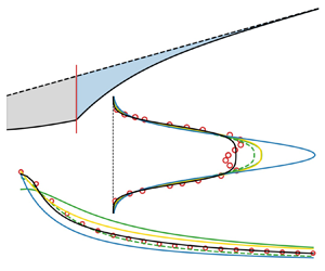
In this study, we build upon the premise of Cheng & Porté-Agel (Reference Cheng and Porté-Agel2018) by developing an analytical solution to the diffusion equation of a passive scalar emitted from a circular disk source, similar to Vahidi & Porté-Agel (Reference Vahidi and Porté-Agel2022), rather than a point source situated at a virtual origin upstream of the turbine. The key in such approach is to provide an analytical form to a streamwise scaling function that ensures that the solution of the diffusion equation conserves linear momentum at all distances downstream of the turbine. The diffusion-based model accounts for the streamwise evolution of the wake profile through a physics-based principle (i.e. diffusion normal to the streamwise direction) rather than the empirical super-Gaussian exponent  $n(x)$ that is not typically related to the physics of the wake. The proposed model also alleviates the need to evaluate Lagrangian statistics from high-fidelity data. Furthermore, super-Gaussian models can provide less accurate results when applied to datasets that were not included in their calibration process, as later shown in § 3. Within a unified framework, diffusion-based wake models offer a higher degree of freedom regarding the wake shape through controlling the distribution of the passive scalar across the source disk.
The rest of the paper is structured as follows. The new wake model is introduced in § 2, where the solution to the diffusion equation is discussed in § 2.1. Discussions on the conservation of linear momentum in the wake region and on far-wake expansion are presented in §§ 2.2 and 2.3, respectively. A modification to the far-wake expansion that takes into account near-wake effects is presented in § 2.4, and the size of the passive scalar disk source is discussed in § 2.5. A step-by-step summary of the proposed model is presented in § 2.6. In § 3, the proposed model is validated against published LES data and experimental measurements, and is compared with other engineering wake models from the literature. The main findings of this paper are discussed in more detail in § 4, and are summarised in § 5. Appendix A suggests a solution to the diffusion equation, and Appendix B derives an analytical solution to a streamwise scaling function that ensures the conservation of linear momentum. A review of the engineering wake models that are considered for comparison in the current study is presented in Appendix C, and some supplementary materials are included in Appendix D.
2. Wake model based on the diffusion of a passive scalar
2.1. Expression for wake shape
In this section, we present a turbine-wake model based on the analogy between the distribution of a turbine's wake normal to the streamwise direction and the diffusion of a passive scalar from a disk source. Following Crank (Reference Crank1979), the diffusion equation from a circular disk source with a uniform initial concentration  $\vartheta _{o}$ is
 \begin{equation} \frac{\vartheta(t,r)}{\vartheta_{o}} = \frac{1}{2\mathcal{D}t} \exp({-r^2/(4\mathcal{D}t)}) \int\nolimits_0^{R_d} r' \exp({-r'^2/(4\mathcal{D}t)}) {\rm I}_0\left(\frac{rr'}{2\mathcal{D}t}\right){\rm d}r', \end{equation}
where  $\vartheta$ is the concentration of the passive scalar, $\mathcal {D}$ is a diffusion coefficient, $t$ is time, $R_d$ is the radius of the disk source, $r$ is the radial distance from the disk's centre and ${\rm I}_{\nu }$ is the modified Bessel function of first kind and order $\nu$. An analogous expression can be written for a self-similar axisymmetric wake of a wind turbine by introducing the length scale $\sigma =\sqrt {2\mathcal {D}t}$, which varies in the streamwise direction. The notion of time in the case of the diffusion of a passive scalar is equivalent to the distance downstream of a turbine. This means that every time instance of the concentration profile of the passive scalar (2.1) corresponds to the wake distribution normal to the streamwise direction at a specific distance downstream of the turbine, both of which are related through some advection wind speed (Cheng & Porté-Agel Reference Cheng and Porté-Agel2018). However, the notion of time in the framework of a turbine's wake is irrelevant since we seek a steady-state solution, and we do not adopt Lagrangian approaches which rely on quantifying the time required for a particle to travel from the turbine to a specific distance downstream of the turbine.
Herein, we assume that the normalised wind-speed deficit  $W$ takes the form
 \begin{align} W(x,r) =1-\frac{u(x,r)}{u_\infty}= C(x) \exp({-r^2/(2\sigma^2)})\underbrace{\frac{1}{\sigma^2} \int\nolimits_0^{R_d} r' \exp({-r'^2/(2\sigma^2)}) {\rm I}_0\left(\frac{rr'}{\sigma^2}\right){\rm d}r'}_{\mathcal{S}(x,r)}, \end{align}
where  $u$ is the streamwise wind speed in the wake region, $u_\infty$ is the free-stream wind speed and $C(x)$ is a scaling function that will be determined from the conservation of linear momentum. Note that $R_d$ is the radius of the passive scalar disk source and is generally different from the turbine's radius $R$ (§ 2.5). Also, the introduced length scale $\sigma$ is not the same as the Gaussian or the super-Gaussian wake widths, but is analogous to these two definitions specific to the assumed wake profile (2.2).
The right-hand side of (2.2) contains a Gaussian function  $\exp ({-r^2/(2\sigma ^2)})$ multiplied by a shaping function $\mathcal {S}(x,r)$ whose role is to have a radially uniform profile near to the wake source and a Gaussian profile in the far wake. To show this, we examine the limiting cases of $\mathcal {S}$ when the length scale $\sigma$ is small (close to the turbine) and when $\sigma$ is large (far from the turbine). As discussed in Appendix A (A11), for a small $\sigma$ the shaping function $\mathcal {S}$ can be approximated by $\exp ({r^2/(2\sigma ^2)})$, which cancels out the Gaussian part in (2.2) resulting in a radially uniform deficit profile. Far away from the turbine, $\sigma$ is large enough to have ${\rm I}_0(rr'/\sigma ^2) \approx 1$, and hence $\mathcal {S}=\mathcal {S}(x)$ is no longer dependent on the radial coordinate $r$, making the profile of $W$ defined by the Gaussian part $\exp ({-r^2/(2\sigma ^2)})$. Therefore, the shaping function $\mathcal {S}$ transitions from having an exponential profile (inverse of a Gaussian profile) to having a radially uniform profile away from the turbine. This transition is caused by the decay of ${\rm I}_0(rr'/\sigma ^2)$ to unity as the wake evolves. Moreover, a similar formulation of (2.2) can be obtained by seeking a rotor-averaged wind-speed deficit for a turbine of radius $R_d$ that is placed in a Gaussian axisymmetric upstream wake and is radially offset from the wake source by a distance $r$ (Ali, Stallard & Ouro Reference Ali, Stallard and Ouro2024b). In this case, the shaping function $\mathcal {S}$ acts as a filter to a background Gaussian field using a circular disk of radius $R_d$. At a far-enough distance from the turbine, the filter size $R_d$ becomes sufficiently smaller than the wake width so that the filtering process does not affect the Gaussian profile of the upstream wake.
To use the wake description provided in (2.2), the integral in  $\mathcal {S}$ needs to be evaluated. This one-dimensional integral can be evaluated using quadrature integration by any mathematical toolbox. However, here, we propose two possible semi-analytical solutions to this integral which require the evaluation of a series, as will be shown. Based on the solution in Appendix A (A7), a possible solution to (2.2) is
 \begin{equation} W(x,r) = C(x) \left(1- \exp({-R_d^2/(2\sigma^2)})\exp({-r^2/(2\sigma^2)}) \sum_{k\ge0} \left(\frac{r}{R_d}\right)^k {\rm I}_{k} \left(\frac{rR_d}{\sigma^2}\right) \right), \end{equation}
which can also be written in terms of the Marcum Q-function (A9) as
 \begin{equation} W(x,r) = C(x) (1-Q_1(r/\sigma, R_d/\sigma)). \end{equation}
When  $\sigma$ is small (i.e. close to the turbine) the summation over $k$ in (2.3) may require a large number of evaluations of modified Bessel functions to converge, although the recursive property of the modified Bessel function should be employed in this case (Abramowitz & Stegun Reference Abramowitz and Stegun1972, p. 376; 9.6.26). Also, the Marcum Q-function may not be available in all mathematical toolboxes. Alternatively, we can use the solution presented by Ali et al. (Reference Ali, Stallard and Ouro2024b) based on the tables by Rosenheinrich (Reference Rosenheinrich2017) to obtain
 \begin{equation} W(x,r) = C(x) \exp({-R_d^2/(2\sigma^2)})\exp({-r^2/(2\sigma^2)}) \varPsi\left(\frac{r}{R_d},\frac{\sigma}{R_d}\right), \end{equation}
where  $\varPsi = \mathcal {S} \exp ({R_d^2/(2\sigma ^2)})$ is defined as
 \begin{equation} \varPsi(\zeta_1,\zeta_2) = {\rm I}_0\!\left(\frac{\zeta_1}{\zeta_2^2}\right)\sum_{k\ge1}\left(\frac{{f}_k\! \left(\zeta_1/\zeta_2\right)}{\left(2\zeta_2^{2}\right)^{k}}\right) - \frac{\zeta_1}{\zeta_2^2} {\rm I}_1 \!\left(\frac{\zeta_1}{\zeta_2^2}\right) \sum_{k\ge1}\left(\frac{{g}_k\!\left(\zeta_1/\zeta_2\right)}{\left(2\zeta_2^{2}\right)^{k}}\right), \end{equation}
and the coefficients  $f_k$ and $g_k$ satisfy the recursions
 \begin{equation} f_k(\alpha) = \frac{f_{k-1}(\alpha) + \alpha^2 g_{k-1}(\alpha)}{k}, \quad g_k(\alpha) = \frac{f_{k}(\alpha) + 2g_{k-1}(\alpha)}{2k}, \end{equation}
with  $f_0=1$ and $g_0=0$. The summations in (2.6) converge rapidly in less than 10 iterations of simple algebraic operations (2.7a,b), and (2.6) requires only two evaluations of the modified Bessel function, which makes it computationally more efficient than (2.3). A Python implementation of (2.6) and (2.7a,b) is available at Ali, Stallard & Ouro (Reference Ali, Stallard and Ouro2024a).
2.2. Conservation of linear momentum
To obtain an expression for the scaling function  $C$ (2.2), we make use of the integral form of the conservation of linear momentum for an axisymmetric wake (Tennekes & Lumley Reference Tennekes and Lumley1972)
 \begin{equation} 2 {\rm \pi}\rho \int\nolimits_{0}^{\infty} u(u_\infty - u) r\,{\rm d}r = \tfrac{1}{2}\rho C_t {\rm \pi}R^2 u_\infty^2, \end{equation}
where  $\rho$ is air density, and $C_t$ is the thrust coefficient of the wind turbine. Detailed derivations to solve (2.8) are available in Appendix B. Equation (2.8) can be simplified to
 \begin{equation} \underbrace{\int\nolimits_{0}^{\infty} r W\,{\rm d}r}_{A_1} - \underbrace{\int\nolimits_{0}^{\infty} r W^2\,{\rm d}r}_{A_2} = R^2 C_t/4. \end{equation}
Following the solution in Appendix B, we have  $A_1=R_d^2 C/2$ and $A_2 \approx R_d^2 C^2 \varLambda /4$, where
 \begin{equation} \varLambda = 2\left({\rm erf}{\left(\frac{R_d}{\sigma}\right)} - \frac{\sigma}{\sqrt{\rm \pi} R_d}\left(1-\exp({-R_d^2/\sigma^2})\right) \right)^2, \end{equation}
with erf being the error function (Ng & Geller Reference Ng and Geller1969; Ali, Stallard & Ouro Reference Ali, Stallard and Ouro2024c). We used an approximation sign for  $A_2$ because $\varLambda$ was not derived directly from $A_2$ but from an alias of $A_2$ (see Appendix B for more details). Therefore, (2.9) can be solved for $C$ as
 \begin{equation} C \approx \frac{1-\sqrt{1- (R/R_d)^2\varLambda C_t}}{\varLambda}. \end{equation}
To complete the model, expressions for the source disk radius  $R_d$ and the length scale $\sigma$ are needed. Thus far, no assumptions were made about the length scale $\sigma$, making (2.2), along with its solutions (2.3)–(2.5), and the scaling function (2.11) generic for any $\sigma (x)$.
2.3. Far-wake expansion
Far from the wake source, high-fidelity simulations and experimental measurements of turbine wakes in turbulent flows show that wakes expand almost linearly in the streamwise direction with a rate that is proportional to the free-stream turbulence intensity (Porté-Agel, Bastankhah & Shamsoddin Reference Porté-Agel, Bastankhah and Shamsoddin2020). Multiple linear expressions have been suggested in the literature based on fitting high-fidelity data (e.g. Bastankhah & Porté-Agel Reference Bastankhah and Porté-Agel2014; Carbajo Fuertes, Markfort & Porté-Agel Reference Carbajo Fuertes, Markfort and Porté-Agel2018; Cathelain et al. Reference Cathelain, Blondel, Joulin and Bozonnet2020). Herein, we use the linear expression suggested by Cathelain et al. (Reference Cathelain, Blondel, Joulin and Bozonnet2020), which provided the best performance against simulations and measurements when combined with (2.2) and (2.11), as shown later in § 3. There are no restrictions to use an expression that was obtained for a super-Gaussian model here with a diffusion-based model (2.2) as long as it is applied in the far wake only, since both the proposed model and the super-Gaussian model approach a Gaussian form far enough downstream (see figure 8). Following Cathelain et al. (Reference Cathelain, Blondel, Joulin and Bozonnet2020), the far-wake length scale  $\sigma _{fw}$ is defined as
 \begin{equation} \sigma_{fw} = \underbrace{\left(0.0119 + 0.18\, T_i\right)}_{k^{*}} x + \underbrace{\left(0.13+ 0.0564 \, C_t\right)\sqrt{\beta}}_{\varepsilon} D, \end{equation}
where  $T_i$ is the free-stream turbulence intensity, $k^*$ is the rate of expansion in the far wake and $D$ is the rotor's diameter. In linear-expansion models, the parameter $\varepsilon$ represents the initial wake width at $x=0$, and the constant $\beta$ is defined as
 \begin{equation} \beta = \frac{1+\sqrt{1-C_t}}{2\sqrt{1-C_t}}. \end{equation}
Due to differences in the flow structure between the near-wake and the far-wake regions (discussed in § 2.4), (2.12) is only applied to the far-wake region, and some modifications are made to  $\sigma _{fw}$ to suit the near wake as follows.
2.4. Near-wake treatment
The near wake is a region of complex structures that are challenging to model analytically. The structure of the flow within this region is three-dimensional, non-symmetric and highly influenced by the geometry of the turbine and the operating tip-speed ratio (Bastankhah & Porté-Agel Reference Bastankhah and Porté-Agel2017). Although adopting engineering wake models in the near wake should be handled with caution, as the assumption of self-similarity is not theoretically valid in this region, we attempt to modify the linear expansion of the far-wake length scale  $\sigma _{fw}$ (2.12) to approximate the near-wake deficit shape and evolution. The streamwise extent of the near wake has been addressed in multiple studies (e.g. Vermeulen Reference Vermeulen1980; Sørensen et al. Reference Sørensen, Mikkelsen, Sarmast, Ivanell and Henningson2014, Reference Sørensen, Mikkelsen, Henningson, Ivanell, Sarmast and Andersen2015; Bastankhah & Porté-Agel Reference Bastankhah and Porté-Agel2016). Herein, we adopt the formulation of the near-wake length $x_{o}$ suggested by Bastankhah & Porté-Agel (Reference Bastankhah and Porté-Agel2016) following Lee & Chu (Reference Lee and Chu2003) for a non-yawed turbine
 \begin{equation} \frac{x_{o}}{D} = \frac{1+\sqrt{1-C_t}}{\sqrt{2}\left(4c_1\,T_i+c_2\left(1-\sqrt{1-C_t}\right)\right)}, \end{equation}
where  $c_1=0.58$ and $c_2=0.154$.
Downstream of a turbine, a free-shear layer is formed between the free-stream flow and the waked flow due to the drop in pressure and wind speed caused by the turbine's momentum extraction (Posa & Broglia Reference Posa and Broglia2021). The evolution of this shear layer depends on the strength and stability of the tip vortices shed by the blades, which partially shield the waked flow from the free-stream flow by reducing momentum and mass transfer across the shear layer (Ivanell et al. Reference Ivanell, Mikkelsen, Sørensen and Henningson2010). If, hypothetically, the tip vortices were to be modelled as an elastic tube that perfectly insulates the waked flow from the free-stream flow, then the pressure difference across this elastic tube would cause the tube to contract, assuming an infinitely long tube in the streamwise direction. However, this does not occur for a turbine's wake as the tip vortices do not perfectly prevent any mass and momentum transfer, leading to a relatively quick pressure recovery shortly downstream of the turbine. On the other hand, a free-shear layer with no resistance for mass and momentum transfer across the layer would have a relatively faster expansion than a shear layer with some resistance. Based on this, we propose an expression for the near-wake length scale  $\sigma _{nw}$ as a superposition of a contraction tendency (in case of perfect wake insulation) and an expansion tendency (in case of no wake insulation)
 \begin{equation} \sigma_{nw} =
\underbrace{\varepsilon R_d \exp({-x/(\tau
x_{o})})}_{\textit{contraction}} + \underbrace{\sigma_{fw}
\left(R_d/R\right) \exp({-R^2/(2\sigma_{fw}^2)})}_{\textit{expansion}},
\end{equation}
\begin{equation} \sigma_{nw} =
\underbrace{\varepsilon R_d \exp({-x/(\tau
x_{o})})}_{\textit{contraction}} + \underbrace{\sigma_{fw}
\left(R_d/R\right) \exp({-R^2/(2\sigma_{fw}^2)})}_{\textit{expansion}},
\end{equation}
where  $\tau =2$, the far-wake length scale $\sigma _{fw}$ and the parameter $\varepsilon$ are defined in (2.12), the near-wake length $x_{o}$ is given by (2.14), $R_d$ is the radius of the source disk and $R$ is the turbine's radius. It is crucial to note that (2.15) is an empirical expression structured to be used specifically with the expression for the far-wake length scale $\sigma _{fw}$ (2.12) and the proposed wake shape (2.2). A generic expression for the near-wake length scale $\sigma _{nw}$ obtained from first principles is beyond the scope of the current study. Furthermore, the parameter $\tau$ in the contraction term of (2.15) was obtained through trial and error against the LES deficit profiles included in § 3 (figure 4), while noting that the model's predictions were not very sensitive to $\tau$ since it only affects the shape of the near wake but has small effect on the far wake (see examples in Appendix D).
Finally, the overall length scale  $\sigma$ is obtained by combining (2.12) and (2.15) using
 \begin{equation} \sigma(x) =
\begin{cases} \sigma_{nw} & \text{if}\ x \leq x_{o},\\
\sigma_{fw} - \exp({\tau(1-x/x_{o})}) \left(\sigma_{fw}-\sigma_{nw}\right) & \text{if}\ x > x_{o}. \end{cases}
\end{equation}
\begin{equation} \sigma(x) =
\begin{cases} \sigma_{nw} & \text{if}\ x \leq x_{o},\\
\sigma_{fw} - \exp({\tau(1-x/x_{o})}) \left(\sigma_{fw}-\sigma_{nw}\right) & \text{if}\ x > x_{o}. \end{cases}
\end{equation}
Similar to (2.15), the suggested blend in (2.16) for  $x>x_{o}$ is empirical and is designed to be used specifically with the expressions for the near- and far-wake length scales (2.15) and (2.12) and the proposed wake shape (2.2).
The streamwise variation of the length scale  $\sigma$ (2.16) is shown in figure 1 for low ( $C_t=0.4$) and high ( $C_t=0.8$) turbine thrust coefficients at different free-stream turbulence intensities. The corresponding near-wake lengths $x_{o}$ (2.14) are shown by vertical dotted lines for each case. Similar to high-fidelity observations (e.g. Troldborg, Sorensen & Mikkelsen Reference Troldborg, Sorensen and Mikkelsen2010), the rate of wake expansion in the near wake (2.15) is slower than that in the far wake (2.12), with the high turbulence cases having higher recovery rates and shorter near-wake regions (figure 1). Moreover, figure 8 (Appendix D) shows the difference between the adopted length scale $\sigma$ (2.16) and the far-wake length scale $\sigma _{fw}$ (2.12) for one of the cases in figure 1. As previously indicated, $\sigma _{fw}$ is used only in the very-far wake where both the proposed wake model (2.2) and the super-Gaussian model of Cathelain et al. (Reference Cathelain, Blondel, Joulin and Bozonnet2020, who developed the expression for $\sigma _{fw}$ in (2.12)) approach a Gaussian wake profile (at $x/D \sim 8$ for the case in figure 8). Otherwise, the near-wake length scale $\sigma _{nw}$ (2.15) and the exponential blend between $\sigma _{nw}$ and $\sigma _{fw}$ (2.16) set the difference between the adopted length scale $\sigma$ and the far-wake length scale $\sigma _{fw}$. Having obtained an expression for the length scale $\sigma$, a solution to (2.2) requires a definition for the radius of the source disk $R_d$, which is discussed in the next section.


2.5. Source disk radius
To have an expression for the source disk radius  $R_d$, we rely on one-dimensional momentum theory by assuming that the pressure recovers quickly to its free-stream value a short distance downstream of the turbine, i.e. when $x \sim 0$ (Narasimhan, Gayme & Meneveau Reference Narasimhan, Gayme and Meneveau2024). This is a simplifying assumption, because in reality the pressure recovers after a finite distance downstream of the turbine, along which the wake expands slightly from its initial size (the turbine's size). Modelling the pressure-recovery region within the proposed low-fidelity wake model is not straightforward, and so this initial wake expansion is modelled in a similar manner to Blondel & Cathelain (Reference Blondel and Cathelain2020) by increasing the size of the source disk.
At  $x=0$, the wake's profile normal to the streamwise direction is fairly uniform, so that we can use the centreline deficit (i.e. $r=0$). From one-dimensional momentum theory, the normalised wind-speed deficit ( $W$) when the pressure recovers to its free-stream value (here at $x=0$) is $1-\sqrt {1-C_t}$ (Burton et al. Reference Burton, Sharpe, Jenkins and Bossanyi2021), which can be equated to the exact solution of (2.2) at the centre of the wake
 \begin{equation} C_{o} \left(1-\exp({-R_d^2/(2\sigma_{o}^2)})\right) = 1-\sqrt{1-C_t}. \end{equation}
In (2.17),  $C_{o} = C(0)$ and $\sigma _{o} = \sigma (0)$ are the scaling function $C$ and the length scale $\sigma$ just downstream of the turbine, respectively. We can use (2.11) at $x=0$ to solve for the disk radius
 \begin{equation} R_d/ R = \sqrt{\frac{C_t}{C_{o}\left(2-\varLambda_{o} C_{o}\right)}}, \end{equation}
where  $\varLambda _{o}=\varLambda (0)$ can be evaluated from (2.10) by replacing $\sigma /R_d$ with $\sigma _{o}/R_d$ which is known from (2.15)
 \begin{equation} \sigma_{o} / R_d = \varepsilon \left(1+2 \exp({-1/(8\varepsilon^2)})\right). \end{equation}
 Similarly,  $C_{o}$ is given by (2.17) by employing (2.19). From (2.18), the ratio $R_d/R$ is dependent on the thrust coefficient $C_t$ only, and this dependency is shown in figure 2, which indicates that the source disk radius $R_d$ is at most approximately 9 % larger than the turbine's radius which occurs at $C_t\sim 0.81$. At higher thrust coefficients, the required disk radius to satisfy the one-dimensional momentum theory (2.17) decreases until it reaches a value of 1 at $C_t\sim 0.95$, after which (2.17) cannot be satisfied. In the shaded region of figure 2, the one-dimensional momentum theory is often replaced by empirical expressions for the relation between the thrust coefficient and the axial induction of the turbine (e.g. Glauert Reference Glauert1926; Buhl Reference Buhl2005; Burton et al. Reference Burton, Sharpe, Jenkins and Bossanyi2021; Liew, Heck & Howland Reference Liew, Heck and Howland2024), because the momentum theory predicts very low wind speeds downstream of the turbine (deficit approaching 100 %) which is not physical. However, this is beyond the scope of the current study, and we suggest limiting (2.18) to values of $C_t$ up to 0.9.
The variation of the ratio between the source disk radius  $R_d$ and the turbine radius $R$ (2.18) with the thrust coefficient $C_t$. The shaded region is where the one-dimensional momentum theory becomes impractical by predicting very low wind speeds (very high deficits approaching 100 %) downstream of the turbine, and is typically replaced by empirical expressions.

2.6. Summary of the proposed model
Thus far, we have determined expressions for all the variables required to solve for the deficit  $W$ (2.2). To summarise, the input data of the proposed wake model are the turbine's thrust coefficient $C_t$, the free-stream turbulence intensity $T_i$ and the turbine's rotor radius $R$. The model predicts the streamwise and radial distributions of the wind-speed deficit downstream of the turbine based on the following steps.
(i) Calculate the source disk radius $R_d$.
(a) From (2.19), calculate the ratio
$\sigma _{o} / R_d$ using the definition of $\varepsilon$ in (2.12).(b) Evaluate
$\varLambda _{o}$ (2.10) and $C_{o}$ (2.17) using the ratio $\sigma _{o} / R_d$ obtained above.(c) Using
$\varLambda _{o}$ and $C_{o}$, the radius of the source disk $R_d$ can be obtained from (2.18).
(iii) Calculate the length scale
$\sigma$.
(a) Calculate the far-wake length scale
$\sigma _{fw}$ from (2.12), where the constant $\beta$ is obtained from (2.13).(b) The near-wake length
$x_{o}$ is obtained from (2.14).(c) Calculate the near-wake length scale
$\sigma _{nw}$ from (2.15).(d) The length scale
$\sigma$ can be obtained from (2.16) based on the streamwise distance $x$ from the turbine relative to the near-wake length $x_{o}$.
(iii) Calculate the streamwise scaling function
$C(x)$.
(iv) Evaluate the radial distribution of the deficit
$W(x,r)$ using one of the following options.
(a) Numerically approximate (2.2) using quadrature integration.
(b) Use the series solution in (2.3).
(c) If the Marcum Q-function is accessible via the used mathematical toolbox, use (2.4).
(d) Use the solution of
$W$ in (2.5) with the aid of the function $\varPsi$ (2.6), which depends on the recursions in (2.7a,b).


3. Validation
In this section, we compare the results of the wake model presented in § 2 with LES and experimental data. Rather than performing a special set of simulations and/or experiments to provide reference data for validation, we employ published numerical and experimental datasets from different research groups.
The first dataset is the LES results of a wind turbine obtained by Vahidi & Porté-Agel (Reference Vahidi and Porté-Agel2022) with an in-house LES code using an actuator disk model in a neutral atmospheric boundary layer flow. They performed a set of simulations for a range of  $T_i$ (5.3 %–14 %) while keeping $C_t$ nearly constant at a value of 0.8. The results of these simulations are labelled ‘EPFL-LES’. The second set is the experimental measurements used by Blondel & Cathelain (Reference Blondel and Cathelain2020) for their validation based on the experiments by Aubrun et al. (Reference Aubrun, Loyer, Hancock and Hayden2013) of a model porous disk in isotropic turbulence, where measurements were taken using wire probes. The experiments comprised cases with high (12 %) and low (5 %) turbulence intensities for different values of $C_t$ within the range 0.45–0.73. We also use the experimental measurements reported by Schreiber et al. (Reference Schreiber, Balbaa and Bottasso2020) based on Wang et al. (Reference Wang, Foley, Nanos, Yu, Campagnolo, Bottasso, Zanotti and Croce2017) for a model turbine operating at $C_t = 0.75$ in a free-stream turbulence intensity of 5 %, where wake measurements were obtained using hot-wire probes and particle image velocimetry. Using these datasets, the present model is compared with the Gaussian model of Bastankhah & Porté-Agel (Reference Bastankhah and Porté-Agel2014, hereafter BPA14), and the super-Gaussian models of Blondel & Cathelain (Reference Blondel and Cathelain2020, hereafter B20), Cathelain et al. (Reference Cathelain, Blondel, Joulin and Bozonnet2020, hereafter C20) and Blondel (Reference Blondel2023, hereafter B23). The details of these models are summarised in Appendix C. It should be noted that the Gaussian model (BPA14) is intended to be used only in the far wake. Therefore, its predictions in the near wake are included for comparison only.
Figure 3 presents a comparison of the hub-height normalised wind-speed deficit predicted by the present model along with the previously mentioned models against the EPFL-LES data. The streamwise variation of the maximum deficit for the same cases of figure 3 is shown in figure 4. The comparison indicates that the present model (black curves) agrees well with the LES results in the near- and far-wake regions. The largest deviations from the LES results are a slight overestimation of the near-wake width in the highest turbulence case (figure 3a), and a slight overestimation of the far-wake deficit in the lowest turbulence case (figure 3s,t). For all other locations, the wake profiles predicted with the new diffusion-based model are in excellent agreement with the LES, and it is noted that none of the considered models capture the observed behaviour in the far wake for the lowest turbulence case (figure 3s,t).
A comparison of hub-height lateral profiles of the normalised wind-speed deficit for different distances downstream against LES results (red circles) obtained from Vahidi & Porté-Agel (Reference Vahidi and Porté-Agel2022), between the present wake model (black curves), the Gaussian wake model (blue curves) of Bastankhah & Porté-Agel (Reference Bastankhah and Porté-Agel2014) and the super-Gaussian wake models of Blondel & Cathelain (Reference Blondel and Cathelain2020) shown by solid-green curves (B20), Cathelain et al. (Reference Cathelain, Blondel, Joulin and Bozonnet2020) shown by yellow curves (C20) and Blondel (Reference Blondel2023) shown by dashed-green curves (B23). All the shown cases have  $C_t=0.8$. Each row represents a case with a different turbulence intensity as indicated. Whenever a model fails in one of the cases, its abbreviation is written with the label ‘NA’, which stands for ‘not applicable’.

Comparing the streamwise variation of the maximum normalised wind-speed deficit  $W_{max}(x)$ against the LES results of Vahidi & Porté-Agel (Reference Vahidi and Porté-Agel2022). The compared models, and their colours, are the same as in figure 3. The vertical dotted lines represent the location of the near wake of each case as defined by (2.14).

Figure 4 shows that the near-wake formulation of the length scale  $\sigma$ introduced in § 2.4 captures the transition from a low recovery rate in the near-wake region to faster recovery further downstream. It is noted that the maximum deficit predicted by the present model is slightly less than that of the LES in the near-wake region of the low turbulence cases (figure 4d,e). This is expected as the maximum deficit in the near-wake region is typically offset from the wake centreline (figure 3m,q), but the present model as well as all the considered models has the maximum deficit at the centre of the wake. Figure 4 shows that the B20 and B23 models were calibrated to match the profiles of the centreline deficit rather than the maximum deficit because both predict an initial increase in the maximum wind-speed deficit rather than the monotonic decrease in the maximum deficit close to the turbine as predicted by LES (e.g. figure 4e). Matching the behaviour of the centreline deficit with a model that does not include the lateral offset of the maximum deficit from the wake centreline can lead to an underestimation of the deficit in the near wake by incorrectly matching the maximum deficit to the centreline deficit. To include the radial offset of the maximum deficit away from the wake centreline in the proposed diffusion-based model, the initial distribution of the passive scalar across the source disk would need to be non-uniform. However, this is beyond the scope of the current study.
Because it is not designed for the near wake, the BPA14 model (blue curves) deviates substantially from LES data in the near-wake region of the cases with  $T_i=9.9\,\%$ (figure 3e) and $T_i=7.7\,\%$ (figure 3i), and is not applicable for the cases with $T_i=6.2\,\%$ (figure 3m) and $T_i=5.3\,\%$ (figure 3q) because of having $\sigma _{g} < R \sqrt {C_t/2}$ (C2). However, for $x \geq 6D$, the Gaussian model matches the deficit of the LES data well except for the cases of high turbulence, where it slightly underestimates the deficit (figure 3b,f). The B20 model (green curves) overestimates the deficit compared with LES in all of the cases and at almost all locations downstream of the turbine except in the near-wake region of the low turbulence cases (figures 3m,q and 4b–e). The model also underestimates the deficit in the near-wake region of the high turbulence cases (figure 3a,e,i). However, the re-calibration of this model as presented by the B23 model (dashed-green curves) enhances the model's predictions significantly. Nonetheless, the B23 model overestimates the far-wake deficit for the low turbulence case (figure 3r–t). Finally, the C20 model (yellow curves) generally overestimates the deficit for the high turbulence cases (figures 3b–d, f–h and 4a,b), except in the near wake where it matches the LES data well (figure 3a). Similar to the Gaussian model, the C20 model is not applicable in the near wake of the low turbulence cases because the quantity in the square root in (C8) is negative.
Figure 5 shows a similar comparison as that in figure 3 but against the porous-disk experiments of Aubrun et al. (Reference Aubrun, Loyer, Hancock and Hayden2013) for a combination of high and low values of  $C_t$ and $T_i$. The present model (black curves) matches the experiments well in all of the cases except in the far wake, where the deficit is underestimated (figure 5h,l,p). However, all the considered models underestimate the far-wake deficit except the B20 model which was calibrated to match this dataset. Also, the present model better captures the wake width compared with the other models, which underestimate the wake width in some of the cases (e.g. figure 5b,c,e,f). The discrepancies between the present model and the porous-disk measurements can be partially attributed to the adopted model of near-wake length $x_{o}$ (2.14) that is calibrated for the wakes of wind turbines (Bastankhah & Porté-Agel Reference Bastankhah and Porté-Agel2016). Using different values for $c_1$ and $c_2$ in (2.14) can mitigate these discrepancies. However, when compared with the experimental measurements of a three-bladed turbine (see figure 6), the proposed model gave good predictions.
Comparing the lateral profiles of the normalised wind-speed deficit of the present model (black curves) and the other Gaussian and super-Gaussian models mentioned in figure 3 with the porous-disk experiments (red circles) of Aubrun et al. (Reference Aubrun, Loyer, Hancock and Hayden2013). Each row represents a case with its  $C_t$ and $T_i$ as indicated, whereas each column is a specific location downstream of the wake source. Whenever a model fails in one of the cases, its abbreviation is written with the label ‘NA’, which stands for ‘not applicable’.

Comparing the lateral profiles of the normalised wind-speed deficit of the present model (black curves) and the other Gaussian and super-Gaussian models mentioned in figure 3 with the measurements in the wake of a model G1 turbine done by Wang et al. (Reference Wang, Foley, Nanos, Yu, Campagnolo, Bottasso, Zanotti and Croce2017) and reported by Schreiber et al. (Reference Schreiber, Balbaa and Bottasso2020). The model turbine operated at  $C_t=0.75$ in a free-stream turbulence intensity of 5 %. Each panel represents a specific location downstream of the turbine as indicated. Whenever a model fails in one of the cases, its abbreviation is written with the label ‘NA’, which stands for ‘not applicable’.

Similar to the LES results in figure 3, the BPA14 model performs poorly in the near wake of the low  $T_i$ and low $C_t$ case (figure 5a), and is not applicable for the low $T_i$ and high $C_t$ case (figure 5e). Also, the BPA14 model underestimates the deficit in the high turbulence cases (third and fourth rows of figure 5), except in the near wake, where it slightly overestimates the deficit (figure 5i,m). The B20 model captures the deficit well in the near wake of the low turbulence case (figure 5a,e), but overestimates the deficit at $x=4D$ (figure 5b,f) and $x=6D$ (figure 5c,g). The B23 model did not enhance the accuracy of the B20 model in this dataset, but gave worse results in the near wake of the high turbulence cases (figure 5i,m). The C20 model consistently overestimates the deficit in the near wake of all the cases of this dataset (first column of figure 5), and underestimates the deficit in the far wake of the low turbulence cases (figure 5d,h).
The last considered dataset is the experimental measurements of a three-bladed turbine (Wang et al. Reference Wang, Foley, Nanos, Yu, Campagnolo, Bottasso, Zanotti and Croce2017), which are presented in figure 6 comparing the lateral profiles of the normalised deficit for the considered wake models (same as in figure 3). The present model captures both the width and the magnitude of the deficit profiles well compared with the experimental measurements (figure 6). As this experiment is at low  $T_i$ and high $C_t$, the BPA14 model is not applicable in the near wake (figure 6a,b), and overestimates the deficit significantly at $x=3D$ (figure 6c) and $x=4D$ (figure 6d). However, the model captures the wake profile well in the far wake (figure 6f). The B20 model captures the magnitude of the deficit well in the near wake but underestimates the width of the wake (figure 6a,b), after which the model consistently overestimates the deficit magnitude (figure 6c–f). The re-calibration in the B23 model did not improve the performance of the B20 model in the near wake, as the B23 model underestimates both the magnitude and the width of the wake (figure 6a,b). The overestimation of the deficit magnitude just after the near wake still persists for the B23 model compared with the B20 model and to the experimental measurements (figure 6c,d), but the overestimation of the deficit in the very far wake is significantly enhanced for the B23 model (figure 6e,f). The C20 model deviates significantly from the experimental measurements in the near wake (figure 6a–c), but performs well in the far wake (figure 6d–f).
4. Discussion
From the validation results shown in § 3, the proposed wake model has been shown to be the most consistent when compared with the reference data of the considered experimental and LES datasets, whereas the other wake models performed well in some cases and poorly in other cases, yielding larger uncertainty. Nonetheless, the diffusion-based model coupled with the expansion model in (2.12) underestimated the far-wake deficit of the high turbulence cases in the porous-disk experiments (figure 5l,p). This discrepancy is partially due to using a near-wake length model (2.14) that is calibrated for turbine wakes, which is supported by the better performance of the proposed model when compared with the measurements in the wake of a three-bladed turbine (figure 6).
It should be noted that the super-Gaussian models, which rely on a set of tuning parameters obtained from fitting high-fidelity data, perform well in the datasets that were included in their calibration process but their accuracy can deteriorate in other datasets. For instance the B20 model performed better than the B23 model in the dataset shown in figure 5 but worse in figures 3 and 6. The C20 model provided good accuracy in the far wake of the high turbulence cases but performed poorly in the near wake, especially for the low turbulence cases. Even the BPA14 model, coupled with the expansion model in (C4), overestimated the wake recovery in the far wake of the high turbulence cases. In contrast, the proposed diffusion-based model matched LES data and experimental measurements, with an acceptable accuracy for a low-fidelity engineering wake model, in both the near- and far-wake regions of all the considered cases with low/high turbulence and low/high turbine thrust coefficients.
The suggested form of the deficit equation (2.2), along with the suggested solutions (2.3)–(2.5) and the streamwise scaling function (2.11) are generic expressions in the sense that they do not depend on any empirical relations. Modelling  $\sigma$ is, however, empirical. The linear expansion of the length scale $\sigma$ in the far wake (2.12) is empirical based on fitting high-fidelity data. Analogously, the near-wake modification discussed in § 2.4 is empirical, as it was not derived from first principles. The condition for obtaining the radius of the source disk (2.17) is also generic as it was obtained from the suggested deficit equation (2.2) and the one-dimensional momentum theory. However, converting this condition to an expression for $R_d$ as a function of the turbine's thrust coefficient depends on the empirical expressions of $\sigma _{fw}$ (far-wake length scale; (2.12)) and $\sigma _{nw}$ (near-wake length scale; (2.15)).
The presented combination of these generic and empirical expressions provides consistent and accurate-enough predictions for a low-fidelity wake model, and outperforms current engineering wake models from the literature for a wide range of turbulence intensities and turbine thrust coefficients. All the considered validation cases in the current study were of a single wake. Nonetheless, the proposed model can be extended to a wind farm by using various wake-superposition methods (e.g. Voutsinas, Rados & Zervos Reference Voutsinas, Rados and Zervos1990; Niayifar & Porté-Agel Reference Niayifar and Porté-Agel2015; Bastankhah et al. Reference Bastankhah, Welch, Martínez-Tossas, King and Fleming2021) and turbine-induced turbulence models (e.g. Crespo & Hernandez Reference Crespo and Hernandez1996). However, we did not include a validation case for a wind farm as farm results are largely influenced by the used wake-superposition method, and the intent of the current study is not to compare superposition methods.
The mathematical analogy between the suggested deficit equation (2.2), and the rotor-averaged deficit of a turbine in a Gaussian axisymmetric upstream wake (Ali et al. Reference Ali, Stallard and Ouro2024b) suggests that the turbine's impact on the flow can be depicted as a moving circular filter through a Gaussian field. The shape of the resulting wake from the filtered field depends on the relative size of the filter and the length scale of the Gaussian field. Far enough from the turbine the filtering process has no effect on the wake shape (i.e. the wake is similar to the Gaussian field), but close to the turbine the filtering process defines the shape of the wake. This way of perceiving the evolution of the wake shape allows for the modelling of more complex wake profiles, such as a double-Gaussian profile, within the same framework of a diffusion-based description of the wake by altering the radial uniformity of the moving filter. In that sense, the Gaussian field is a potential field for different wake shapes and sizes depending on the shape, size and nature of the applied filter.
5. Summary
A new engineering wake model was presented and validated based on the analogy between the profile of a turbine's wake normal to the streamwise direction and the diffusion of a passive scalar from a disk source. The proposed model guarantees that linear momentum is conserved at all locations downstream of the turbine, and it naturally takes into account the evolution of the wake shape from a top-hat profile in the near wake to a Gaussian profile far downstream of the turbine. The model relies on a far-wake linear-expansion model from the literature, but introduces further adjustments to this linear expansion to describe the lower rate of wake expansion observed in the near-wake region. The size of the source disk of the passive scalar is determined from one-dimensional momentum theory based on the assumption of a fully recovered pressure field over a short distance downstream of the turbine.
Three datasets were used to validate the proposed wake model, including high-fidelity LES data and experimental measurements in the wake of a porous disk and a model turbine. The diffusion-based model captured the wake profiles and the streamwise evolution of the maximum deficit well when compared with the reference datasets, with a slight deviation against the far-wake porous-disk measurements in the case of high free-stream turbulence. A comparison with other widely used engineering wake models from the literature, including Gaussian and super-Gaussian models, showed that the new diffusion-based wake model offers a more consistent performance over a wide range of turbulence intensities and turbine thrust coefficients. Super-Gaussian wake models performed well when applied to datasets that were included in their calibration process, but reduced performance is observed when applied to other datasets.
Importantly, the streamwise evolution of the wake shape is accounted for in the proposed model through a physics-based principle (wake diffusion normal to the streamwise direction) rather than an empirical super-Gaussian exponent. Wake models in the literature typically assume a constant deficit in the near-wake region, whereas the introduced empirical expression for near-wake expansion is not restricted to this simplification and is better aligned with LES near-wake results. The presented framework in this study can be extended to more complex wake shapes to account for the near-wake radial offset of the maximum deficit by controlling the initial distribution of the passive scalar. The analytical solutions presented in the current study are not exclusive to turbine wakes but are useful to other applications relying on similar integrals.
Acknowledgements
The authors would like to thank Professor S. Utyuzhnikov from the University of Manchester for his valuable suggestions regarding the mathematical derivations in this study. The authors also appreciate the shared datasets provided by Professor F. Porté-Agel from École Polytechnique Fédérale de Lausanne (EPFL) and by Dr F. Blondel from IFP Energies nouvelles.
Funding
This research was partly supported by the Supergen Offshore Renewable Energy Hub, funded by the Engineering and Physical Science Research Council (EPSRC) grant nos EP/S000747/1 and EP/Y016297/1. The present work has been partly supported by the Dame Kathleen Ollerenshaw Fellowship that P.O. holds at the University of Manchester.
Declaration of interests
The authors report no conflict of interest.
Appendix A. Emphasis on the integral in the diffusion equation
In this appendix, we present a series solution to the integral in (2.2). First, we make use of the improper version of the integral to write (Gradshteyn & Ryzhik Reference Gradshteyn and Ryzhik2007, p. 707; 6.633-4)
 \begin{equation} \int\nolimits_0^{\infty} r' \exp({-r'^2/(2\sigma^2)}){\rm I}_0\left(\frac{rr'}{\sigma^2}\right){\rm d}r' = \sigma^2 \exp({r^2/(2\sigma^2)}), \end{equation}
which we can use to re-write the integral of interest as
 \begin{align} &\int\nolimits_0^{R_d} r' \exp({-r'^2/(2\sigma^2)}){\rm I}_0\left(\frac{rr'}{\sigma^2}\right){\rm d}r'\nonumber\\ &\quad = \sigma^2 \exp({r^2/(2\sigma^2)}) - R_d^2 \underbrace{ \int\nolimits_1^{\infty} r'' \exp({-r''^2 R_d^2/(2\sigma^2)}){\rm I}_0\left(\frac{rr'' R_d}{\sigma^2}\right){\rm d}r''}_{\mathcal{G}}, \end{align}
where  $r'' = r'/R_d$. We can also make use of the multiplication theorem of the modified Bessel function (Abramowitz & Stegun Reference Abramowitz and Stegun1972, p. 377; 9.6.51) to write
 \begin{equation} {\rm I}_0\left(\frac{rr'' R_d}{\sigma^2}\right) = \sum_{k\ge0} \frac{1}{k!} \left(r''^2-1\right)^k \left(\frac{r R_d}{2\sigma^2}\right)^k {\rm I}_{k} \left(\frac{r R_d}{\sigma^2}\right), \end{equation}
and hence
 \begin{equation} \mathcal{G} = \sum_{k\ge0} \frac{1}{k!} \left(\frac{rR_d}{2\sigma^2}\right)^k {\rm I}_{k} \left(\frac{rR_d}{\sigma^2}\right) \underbrace{ \int\nolimits_1^{\infty} r'' \left(r''^2-1\right)^k \exp({-r''^2 R_d^2/(2\sigma^2)})\,{\rm d}r'' }_{{\mathcal{F}_k}}. \end{equation}
Applying integration by parts to  ${\mathcal {F}_k}$ leads to the following recursion:
 \begin{equation} {\mathcal{F}_k} = \frac{2k\sigma^2}{R_d^2} {\mathcal{F}_{k-1}}, \end{equation}
whose solution is  $k! (2\sigma ^2/R_d^2)^k {\mathcal {F}_0}$, where
 \begin{equation} {\mathcal{F}_0} = \int\nolimits_1^{\infty} r'' \exp({-r''^2 R_d^2/(2\sigma^2)})\,{\rm d}r'' = \frac{\sigma^2}{R_d^2} \exp({-R_d^2/(2\sigma^2)}). \end{equation}
Inserting the solution of  $\mathcal {F}_{k}$ into (A4) and then into (A2) gives
 \begin{align} &\int\nolimits_0^{R_d} r' \exp({-r'^2/(2\sigma^2)}){\rm I}_0\left(\frac{rr'}{\sigma^2}\right){\rm d}r'\nonumber\\ &\quad =\sigma^2 \exp({r^2/(2\sigma^2)}) - \sigma^2 \exp({-R_d^2/(2\sigma^2)})\sum_{k\ge0} \left(\frac{r}{R_d}\right)^k {\rm I}_{k} \left(\frac{rR_d}{\sigma^2}\right). \end{align}
Moreover, we can relate the generating function in (A7) to the Marcum Q-function  $Q_M(a,b)$ through (Proakis Reference Proakis1983, p. 44; 2-1-123)
 \begin{equation} \sum_{k\ge0} \left(\frac{r}{R_d}\right)^k {\rm I}_{k} \left(\frac{rR_d}{\sigma^2}\right) = \exp({r^2/(2\sigma^2)}) \exp({R_d^2/(2\sigma^2)}) Q_1(r/\sigma, R_d/\sigma), \end{equation}
and hence
 \begin{equation} \int\nolimits_0^{R_d} r' \exp({-r'^2/(2\sigma^2)}){\rm I}_0\left(\frac{rr'}{\sigma^2}\right){\rm d}r'= \sigma^2 \exp({r^2/(2\sigma^2)}) (1-Q_1(r/\sigma, R_d/\sigma)). \end{equation}
The Marcum Q-function is found in some, but not all, mathematical toolboxes, and hence (A7) can still be useful. Also, (A7) can be used to examine the limiting behaviour of the shaping function  $\mathcal {S}$ defined in (2.2) as follows. Close to the wake source, the characteristic length $\sigma$ is small, making the argument of the modified Bessel function sufficiently large to use the approximation (Abramowitz & Stegun Reference Abramowitz and Stegun1972, p. 377; 9.7.1)
 \begin{equation} {\rm I}_{k} \left(\frac{rR_d}{\sigma^2}\right) \sim \sigma \frac{\exp({rR_d/\sigma^2})}{\sqrt{2{\rm \pi} r R_d}} \left(1+O(\sigma^2)\right). \end{equation}
Using this approximation along with (A7) and  $\lim \limits_{\sigma \to 0}\sigma \exp ({-c/\sigma ^2})=0$, we can approximate $\mathcal {S}$ for a small $\sigma$ as
 \begin{equation} \mathcal{S}|_{\sigma \ll} \approx \exp({r^2/(2\sigma^2)}). \end{equation}
A similar result can be obtained from (A9) using the fact that the first-order Marcum Q-function  $Q_1(a,b)$ vanishes for large values of $b$, which occurs when $\sigma$ is small as $b=R_d/\sigma$.
Appendix B. Conservation of linear momentum
In this appendix, we present a derivation for the streamwise scaling function  $C(x)$ to ensure that the wake form introduced in (2.2) conserves linear momentum. From the integral form of the conservation of linear momentum in the wake of a turbine, we have (Tennekes & Lumley Reference Tennekes and Lumley1972)
 \begin{equation} 2 {\rm \pi}\rho \int\nolimits_{0}^{\infty} u(u_\infty - u) r\,{\rm d}r = \tfrac{1}{2}\rho C_t {\rm \pi}R^2 u_\infty^2, \end{equation}
where  $\rho$ is the air density, $C_t$ is the thrust coefficient, $R$ is the turbine's radius, $u_\infty$ is the free-stream wind speed, $u$ is the wind speed in the turbine's wake and $r$ is a radial coordinate. By making use of the definition $W=1-u/u_\infty$, (B1) becomes
 \begin{equation} \underbrace{\int\nolimits_{0}^{\infty} r W\,{\rm d}r}_{A_1} - \underbrace{\int\nolimits_{0}^{\infty} r W^2\,{\rm d}r}_{A_2} = R^2 C_t/4. \end{equation}
From (2.2), the normalised wind-speed deficit  $W$ is
 \begin{equation} W = C\exp({-r^2/(2\sigma^2)}) \frac{1}{\sigma^2} \int\nolimits_0^{R_d} r' \exp({-r'^2/(2\sigma^2)}) {\rm I}_0\left(\frac{rr'}{\sigma^2}\right){\rm d}r', \end{equation}
and the corresponding integrals  $A_1$ and $A_2$ are evaluated as follows.
B.1. The integral $A_1$

The integral  $A_1$ is
 \begin{equation} A_1 = \frac{C}{\sigma^2} \int\nolimits_{0}^{\infty} r \exp({-r^2/(2\sigma^2)}) \left(\int\nolimits_{0}^{R_d} r' \exp({-r'^2/(2\sigma^2)}){\rm I}_0\left(\frac{rr'}{\sigma^2}\right){\rm d}r'\right) {\rm d}r, \end{equation}
which can be re-arranged as
 \begin{equation} A_1 = \frac{C}{\sigma^2} \int\nolimits_{0}^{R_d} r' \exp({-r'^2/(2\sigma^2)}) \left(\int\nolimits_{0}^{\infty} r \exp({-r^2/(2\sigma^2)}){\rm I}_0\left(\frac{rr'}{\sigma^2}\right) {\rm d}r\right){\rm d}r'. \end{equation}
The improper integral in (B5) is given by (A1), and hence,
 \begin{equation} A_1 = C \int\nolimits_{0}^{R_d} r'\,{\rm d}r' = \frac{1}{2}R_d^2 C. \end{equation}
B.2. The integral $A_2$

As for the integral  $A_2$
$A_2$
 \begin{align} A_2 &= \frac{C^2}{\sigma^4}\int\nolimits_{0}^{\infty} r \exp({-r^2/\sigma^2}) \nonumber\\ &\quad \times\left(\int\nolimits_{0}^{R_d} \eta_1 \exp({-\eta_1^2/(2\sigma^2)}){\rm I}_0\left(\frac{r\eta_1}{\sigma^2}\right){\rm d}\eta_1 \int\nolimits_{0}^{R_d} \eta_2 \exp({-\eta_2^2/(2\sigma^2)}){\rm I}_0\left(\frac{r\eta_2}{\sigma^2}\right){\rm d}\eta_2\right){\rm d}r. \end{align}
The dummy variable  $r'$ in (2.2) was replaced with the dummy variables $\eta _1$ and $\eta _2$ for each instance of this integral in $W^2$. We could not obtain a mathematically exact solution of $A_2$. However, we will present two approaches to obtain an approximate expression for $A_2$.
B.2.1. Approach 1
By re-arranging (B7), we get
 \begin{align} A_2 &=
\frac{C^2}{\sigma^4} \int\nolimits_{0}^{R_d}
\int\nolimits_{0}^{R_d} \eta_1 \eta_2
\exp\left({-\left(\eta_1^2+\eta_2^2\right)/(2\sigma^2)}\right)\nonumber\\
&\quad \times\left(\int_{0}^{\infty} r
\exp({-r^2/\sigma^2}) {\rm
I}_0\left(\frac{r\eta_1}{\sigma^2}\right) {\rm
I}_0\left(\frac{r\eta_2}{\sigma^2}\right){\rm
d}r\right){\rm d}\eta_1 \,{\rm d}\eta_2.
\end{align}
\begin{align} A_2 &=
\frac{C^2}{\sigma^4} \int\nolimits_{0}^{R_d}
\int\nolimits_{0}^{R_d} \eta_1 \eta_2
\exp\left({-\left(\eta_1^2+\eta_2^2\right)/(2\sigma^2)}\right)\nonumber\\
&\quad \times\left(\int_{0}^{\infty} r
\exp({-r^2/\sigma^2}) {\rm
I}_0\left(\frac{r\eta_1}{\sigma^2}\right) {\rm
I}_0\left(\frac{r\eta_2}{\sigma^2}\right){\rm
d}r\right){\rm d}\eta_1 \,{\rm d}\eta_2.
\end{align}
The solution of the improper integral in (B8) is (Gradshteyn & Ryzhik Reference Gradshteyn and Ryzhik2007, p. 707; 6.633-4)
 \begin{equation}
\int\nolimits_{0}^{\infty} r \exp({-r^2/\sigma^2}) {\rm
I}_0\left(\frac{r\eta_1}{\sigma^2}\right) {\rm
I}_0\left(\frac{r\eta_2}{\sigma^2}\right){\rm d}r =
\frac{1}{2}\sigma^2
\exp\left({\left(\eta_1^2+\eta_2^2\right)/(4\sigma^2)}\right) {\rm
I}_0\left(\frac{\eta_1\eta_2}{2\sigma^2}\right),
\end{equation}
\begin{equation}
\int\nolimits_{0}^{\infty} r \exp({-r^2/\sigma^2}) {\rm
I}_0\left(\frac{r\eta_1}{\sigma^2}\right) {\rm
I}_0\left(\frac{r\eta_2}{\sigma^2}\right){\rm d}r =
\frac{1}{2}\sigma^2
\exp\left({\left(\eta_1^2+\eta_2^2\right)/(4\sigma^2)}\right) {\rm
I}_0\left(\frac{\eta_1\eta_2}{2\sigma^2}\right),
\end{equation}
and hence (B8) simplifies to
 \begin{equation} A_2 = \frac{R_d^2 C^2}{2\tilde{\sigma}^2} \int\nolimits_{0}^{1} \int\nolimits_{0}^{1} \xi_1 \xi_2 \exp\left({-\left(\xi_1^2+\xi_2^2\right)/(4\tilde{\sigma}^2)}\right) {\rm I}_0\left(\frac{\xi_1\xi_2}{2\tilde{\sigma}^2}\right){\rm d}\xi_1 \,{\rm d}\xi_2, \end{equation}
where  $\xi _1 = \eta _1/R_d$, $\xi _2 = \eta _2/R_d$ and $\tilde {\sigma } = \sigma /R_d$. Equation (B10) contains an integral over a unit square in the first quadrant of the $\xi _1-\xi _2$ space. We can split this integral into $A_2'$, which is the integral over the quarter of the unit circle inscribed in the unit square of integration, and $A_2''$, which is the integral over the left-over area (i.e. $A_2 = A_2' + A_2''$). By introducing the polar coordinates $r_\xi -\theta _\xi$ that satisfy $\xi _1=r_\xi \cos {\theta _\xi }$ and $\xi _2=r_\xi \sin {\theta _\xi }$, the integral $A_2'$ becomes
 \begin{equation} A_2' = \frac{R_d^2 C^2}{4\tilde{\sigma}^2} \int\nolimits_{0}^{1} r_\xi^3 \exp({-r_\xi^2/(4\tilde{\sigma}^2)}) \int\nolimits_{0}^{{\rm \pi}/2} \sin{(2\theta_\xi)}\, {\rm I}_0\left(\frac{r_\xi^2 \sin{(2\theta_\xi)}}{4\tilde{\sigma}^2}\right){\rm d}\theta_\xi\,{\rm d}r_\xi. \end{equation}
The solution to inner integral in (B11) (over  $\theta _\xi$) is $4\tilde {\sigma }^2r_\xi ^{-2}\sinh {(0.25\, r_\xi ^2\tilde {\sigma }^{-2})}$ (Gradshteyn & Ryzhik Reference Gradshteyn and Ryzhik2007, p. 725; 6.681-8), and hence
 \begin{align} A_2' &= R_d^2 C^2 \int\nolimits_{0}^{1} r_\xi \exp({-r_\xi^2/(4\tilde{\sigma}^2)}) \sinh{\left(\frac{r_\xi^2}{4\tilde{\sigma}^2}\right)} {\rm d}r_\xi \nonumber\\ &= \frac{R_d^2 C^2}{4} \left(1-\frac{2\sigma^2}{R_d^2}\left(1-\exp({-R_d^2/(2\sigma^2)})\right)\right). \end{align}
As for the integral  $A_2''$, we have
 \begin{equation} A_2'' = \frac{R_d^2 C^2}{4\tilde{\sigma}^2} \int\nolimits_{0}^{{\rm \pi}/2} \sin{(2\theta_\xi)} \int\nolimits_{1}^{\sec{\theta_{\xi}}} r_\xi^3 \exp({-r_\xi^2/(4\tilde{\sigma}^2)}) \, {\rm I}_0\left(\frac{r_\xi^2 \sin{(2\theta_\xi)}}{4\tilde{\sigma}^2}\right){\rm d}r_\xi\,{\rm d}\theta_\xi. \end{equation}
The integral over  $r_\xi$ in (B13) is not straightforward to solve analytically. However, using numerical evaluation of the integral $A_2$ (B7) and (B12), we can show that
 \begin{align} A_2''&\approx \frac{R_d^2 C^2}{8} \left(1-\frac{\sigma^2}{R_d^2}\left(1-\exp({-R_d^2/\sigma^2})\right)\right) \nonumber\\ &\quad + \frac{R_d^2 C^2}{10} \left(1-\frac{23\sigma^2}{R_d^2}\left(1-\exp({-R_d^2/(22\sigma^2)})\right)\right), \end{align}
and hence  $A_2 \approx R_d^2 C^2 \lambda /4$, where
 \begin{align} \lambda &= 1.9 - \frac{2\sigma^2}{R_d^2}\left(1-\exp({-R_d^2/(2\sigma^2)})\right) -\frac{\sigma^2}{2R_d^2}\left(1-\exp({-R_d^2/\sigma^2})\right) \nonumber\\ &\quad - \frac{46\sigma^2}{5R_d^2}\left(1-\exp({-R_d^2/(22\sigma^2)})\right). \end{align}
B.2.2. Approach 2
The difficulty in solving the integral  $A_2$ in (B7) analytically arises in part due to the presence of the modified Bessel function ${\rm I}_{0}$, which emerges from the integration of a Gaussian function over a circular disk. Geometrically, the integral $A_2$ represents the volume between the surface $W^2(\kern0.7pt y,z)$ and the $y$–
$y$– $z$ plane (scaled by $2{\rm \pi}$ for the azimuthal integration over $\theta$). This volume is an integral quantity and hence is not exclusive to a specific shape of the disk source, but can be obtained from other shapes by appropriate sizing and scaling relative to the circular disk source. Unlike the circular case, the equations for a rectangular disk source can be solved exactly. Given that we are considering an axisymmetric wake, modelled through the diffusion of a passive scalar from a uniform circular disk source, we seek an approximate solution for the integral $A_2$ by using a uniform square disk source with a side length $2l$. This approximation is intended solely for solving $A_2$ and is not related to the presented wake model which assumes a circular disk source. We define $\tilde {W}$ as the normalised wind-speed deficit due to a square disk source, and seek to evaluate $\tilde {A}_2$ such that
 \begin{equation} \tilde{A}_2 = \int\nolimits_{-\infty}^{\infty} \int\nolimits_{-\infty}^{\infty} \tilde{W}^2\,{{\rm d}y}\,{\rm d}z. \end{equation}
For a square disk source,  $\tilde {W}$ can be expressed in terms of the error function (erf) as (Ng & Geller Reference Ng and Geller1969; Crank Reference Crank1979)
 \begin{equation} \tilde{W} = \frac{{\rm \pi} C}{2} \left[{\rm erf}\left(\frac{l-y}{\sqrt{2}\sigma}\right) + {\rm erf}\left(\frac{l+y}{\sqrt{2}\sigma}\right)\right] \left[{\rm erf}\left(\frac{l-z}{\sqrt{2}\sigma}\right) + {\rm erf}\left(\frac{l+z}{\sqrt{2}\sigma}\right)\right]. \end{equation}
Since  $C$ and $\sigma$ are functions of the streamwise direction $x$ but are not functions of $y$ and $z$, they are the assumed to be same for the circular and square disk sources. Because $y$ and $z$ are separable in (B17), we can consider only one of them in the integration over the $y$–
$y$– $z$ plane (B16), and the other integral would be the same. For the $y$ direction, the integral in (B16) yields an integration in the form
 \begin{equation} \mathcal{M}(a) = \sqrt{2}\sigma \int\nolimits_{-\infty}^{\infty} \left({\rm erf}\left(a-\eta\right) + {\rm erf}\left(a+\eta\right)\right)^2{\rm d}\eta, \end{equation}
where  $a=l/(\sqrt {2}\sigma )$, and $\eta =y/(\sqrt {2}\sigma )$. According to Ali et al. (Reference Ali, Stallard and Ouro2024c),
 \begin{equation} \int\nolimits_{-\infty}^{\infty} \left(\textrm{erf}(a-\eta) + \textrm{erf}(a+\eta)\right)^2{\rm d}\eta =8 \left(a\,\textrm{erf}(\sqrt{2}a) + \frac{\exp({-2a^2})-1}{\sqrt{2{\rm \pi}}} \right), \end{equation}
and hence
 \begin{equation} \tilde{A}_2 = 16{\rm \pi} C^2 l^2 \left(\sqrt{\rm \pi}\,{\rm erf}{\left(\frac{l}{\sigma}\right)} - \frac{\sigma}{l}\left(1-\exp({-l^2/\sigma^2})\right) \right)^2. \end{equation}
Through a comparison with numerical evaluation of  $A_2$ (B7) and exploiting the form in (B20) assuming that $l=R_d$, we can show that $A_2 \approx R_d^2 C^2 \varLambda /4$, where
 \begin{equation} \varLambda = 2\left({\rm erf}{\left(\frac{R_d}{\sigma}\right)} - \frac{\sigma}{\sqrt{\rm \pi} R_d}\left(1-\exp({-R_d^2/\sigma^2})\right) \right)^2. \end{equation}
B.3. An expression for the scaling function $C$

Figure 7 shows a comparison between the approximate solutions of the integral  $A_2$: $\lambda$ (B15) and $\varLambda$ (B21) against numerical evaluation of $A_2$. From this comparison, we adopt the $\varLambda$ function as an approximate solution to $A_2$. Having evaluated the integrals $A_1$ (B6) and $A_2$ (B21), the conservation of linear momentum (B2) simplifies to $\varLambda C^2 - 2C + (R/R_d)^2 C_t = 0$, whose solution is
 \begin{equation} C \approx \frac{1-\sqrt{1-(R/R_d)^2 \varLambda C_t}}{\varLambda}. \end{equation}
We use the approximation symbol in (B22) because the integral  $A_2$ is not mathematically exact in the sense that we could not derive (B21) directly from the main expression of $A_2$ (B7), but from an alias of $A_2$ (B16).


Appendix C. Review of analytical wake models
In this appendix we review some engineering wake models from the literature that are included in the comparisons of § 3. We mainly focus on the Gaussian model of Bastankhah & Porté-Agel (Reference Bastankhah and Porté-Agel2014) and the super-Gaussian models of Blondel & Cathelain (Reference Blondel and Cathelain2020), Cathelain et al. (Reference Cathelain, Blondel, Joulin and Bozonnet2020) and Blondel (Reference Blondel2023).
C.1. Gaussian wake
In the Gaussian model of Bastankhah & Porté-Agel (Reference Bastankhah and Porté-Agel2014), the normalised wind-speed deficit  $W_{g}$ (the subscript ${g}$ means Gaussian) is expressed as
 \begin{equation} W_{g} = C_{g}(x) \exp({-r^2/(2\sigma_{g}^2)}), \end{equation}
where the scaling function  $C_{g}(x)$ is
 \begin{equation} C_{g}(x) = 1-\sqrt{1-\frac{C_t}{8\left(\sigma_{g}/D\right)^2}}, \end{equation}
and the length scale  $\sigma _{g}$ expands linearly in the streamwise direction following
 \begin{equation} \sigma_{g} = k^{*}_{g} x + \varepsilon_{g} D. \end{equation}
The rate of wake expansion  $k^{*}_{g}$ is assumed to linearly depend on the free-stream turbulence intensity $T_i$
$T_i$
 \begin{equation} k^{*}_{g} = 0.003678 + 0.3837\, T_i, \end{equation}
and the initial wake width  $\varepsilon _{g}$ is
 \begin{equation} \varepsilon_{g} = 0.2 \sqrt{\beta}, \end{equation}
where
 \begin{equation} \beta = \frac{1+\sqrt{1-C_t}}{2\sqrt{1-C_t}}. \end{equation}
C.2. Super-Gaussian wake
In a super-Gaussian model, the normalised wind-speed deficit  $W_{sg}$ (the subscript ${sg}$ means super-Gaussian) is
 \begin{equation} W_{sg} = C_{sg}(x) \exp({-r^n/(2\sigma_{sg}^2)}), \end{equation}
where  $n$ is a super-Gaussian exponent, $C_{sg}$ is a super-Gaussian scaling function and $\sigma _{sg}$ is a characteristic length scale of the super-Gaussian model. Note that $n$,
$n$,  $C_{sg}$ and $\sigma _{sg}$ will have the same formulation for all the considered super-Gaussian models, and hence were not given special subscripts although their tuneable parameters will have different values, as will be discussed. Blondel & Cathelain (Reference Blondel and Cathelain2020) derived an expression for $C_{sg}(x)$ based on the conservation of linear momentum to be
 \begin{equation} C_{sg}(x) = 2^{-1+2/n} - \sqrt{2^{-2+4/n} - \frac{n C_t}{16 \varGamma(2/n)\,(\sigma_{sg}/D)^{4/n}}}, \end{equation}
where  $\varGamma$ is the gamma function. The super-Gaussian exponent $n$ takes the form
 \begin{equation} n = a_{f} \exp({b_{f} x}) + c_{f}, \end{equation}
where  $a_{f}$, $b_{f}$ and $c_{f}$ are tuneable parameters. The characteristic length scale $\sigma _\textrm {sg}$ is
 \begin{equation} \sigma_{sg} = \left(a_{s} T_i + b_{s}\right) x + c_{s} \sqrt{\beta}D, \end{equation}
where  $a_{s}$, $b_{s}$ and $c_{s}$ are tuneable parameters, and $\beta$ is given by (C6). The six tuneable parameters $a_{f}$, $b_{f}$, $c_{f}$, $a_{s}$, $b_{s}$ and $c_{s}$ are obtained from fitting LES data differently for each of the considered super-Gaussian models, as summarised in table 1. In the model of Blondel & Cathelain (Reference Blondel and Cathelain2020), all six parameters have numeric values as listed in the first row of table 1. However, in the model of Cathelain et al. (Reference Cathelain, Blondel, Joulin and Bozonnet2020), the parameters $b_{f}$ and $c_{s}$ are defined to be functions of $T_i$ and $C_t$, respectively,
 $$\begin{gather} \left(b_{f}\right)_{{C20}} = 1.59\exp({-23.31\, T_i}) - 2.15 \end{gather}$$
 $$\begin{gather}\left(c_{s}\right)_{{C20}} = 0.0564\, C_t + 0.13 . \end{gather}$$
Also,  $a_{f}$ is obtained from one-dimensional momentum theory (Burton et al. Reference Burton, Sharpe, Jenkins and Bossanyi2021) using root finding to ensure that the maximum deficit at the start of the wake equals the axial induction of the turbine $a=0.5(1-\sqrt {1-C_t})$. In the model of Blondel (Reference Blondel2023), the parameters $a_{f}$, $b_{f}$ and $c_{s}$ are defined as
 $$\begin{gather} \left(a_{f}\right)_{{B23}} =-8.2635\, C_t^3 + 8.5939\, C_t^2 - 8.9691\, C_t + 10.7286 \end{gather}$$
 $$\begin{gather}\left(b_{f}\right)_{{B23}} = 1.68\exp({-25.98\,T_i})-1.06 \end{gather}$$
 $$\begin{gather}\left(c_{s}\right)_{{B23}} = 0.1\, C_t + 0.1 . \end{gather}$$
Appendix D. Supplementary material
In this appendix we include some supplementary figures to the main text. Figure 8 shows the streamwise profile of the adopted length scale  $\sigma$ (2.16) and the far-wake length scale $\sigma _{fw}$ (2.12) for an exemplary case of $C_t=0.8$ and $T_i=11\,\%$. The near-wake adjustment due to the definition of $\sigma _{nw}$ (2.15) is indicated by the grey-shaded region, whereas the role of the exponential blend between $\sigma _{nw}$ and $\sigma _{fw}$ (2.16) in the far wake is indicated by the blue-shaded region. The length scale $\sigma$ approaches $\sigma _{fw}$ in the very-far wake where both the proposed wake model (2.2) and the super-Gaussian model (Cathelain et al. Reference Cathelain, Blondel, Joulin and Bozonnet2020, for which $\sigma _{fw}$ in (2.12) is designed) approach a Gaussian wake profile.
The streamwise evolution of the length scale  $\sigma$ (solid black curve) for $C_t=0.8$ and $T_i=11\,\%$. The range of the near wake $x_{o}$ (2.14) is shown by a vertical red line. The far-wake length scale $\sigma _{fw}$ (2.12) is shown by a dashed line. The difference between $\sigma _{fw}$ and the adopted expression for $\sigma$ (2.16) is shaded in grey for the near-wake region and in blue for the far-wake region. The parameter $\tau =2$ as outlined in § 2.4.

The expression for the near-wake length scale  $\sigma _{nw}$ (2.15) is formed by the superposition of a contraction and an expansion tendencies. The parameter $\tau$ in the contraction term was obtained empirically using the LES deficit profiles of figure 3, as outlined in § 2.4. Figure 9 presents an exemplary sensitivity analysis of the parameter $\tau$ for the case of $T_i=6.2\,\%$ (fourth row) of the LES deficit profiles in figure 3. Figure 9 indicates a slight variation in the deficit $W$ for the three tested values of $\tau$. When $\tau$ was halved from 2 to 1 (50 % drop), the increase in the deficit $W$ was approximately 6 % of the free-stream wind speed $u_\infty$ at $x/D=2$, and approximately 6.6 % of $u_\infty$ at $x/D=6$. Moreover, when $\tau$ was doubled from 2 to 4 (a 100 % increase), the deficit $W$ dropped by approximately 2 % of $u_\infty$ at $x/D=2$ and by approximately 5 % of $u_\infty$ at $x/D=6$. These variations occurred for the near-wake case ( $x/D=2$) and for $x/D=6$ along the wake's centreline, but considering the full deficit profile normal to the streamwise direction $\tau =2$ gives best agreement. The other cases show negligible differences.
Sensitivity of the proposed wake model to the parameter  $\tau$ in the expression for $\sigma _{nw}$ (2.15) and in the exponential blend between $\sigma _{nw}$ and $\sigma _{fw}$ (2.16). Three values are tested: $\tau =1$ (blue), $\tau =2$ (black; original value in (2.15)) and $\tau =4$ (green) against LES results (red). Shown is the fourth row ( $T_i=6.2\,\%$) of the LES deficit profiles indicated in figure 3.


 Open access

