


1 Introduction
The semantics of first-order logic is based on the inductively defined concept of an assignment satisfying a formula in a given model. In a more general approach, called team semantics, the basic concept is that of a set of assignments satisfying a formula in a model. This allows consideration of new atomic formulas such as “x is totally determined by
 $y_1,\ldots ,y_n$
” and “
$y_1,\ldots ,y_n$
” and “
 $x_1,\ldots ,x_n$
are independent of
$x_1,\ldots ,x_n$
are independent of
 $y_1,\ldots ,y_m$
”. Such constraints on variables appear throughout sciences but in experimental sciences in particular. In this article, we apply team semantics to investigate determinism and independence concepts in quantum physics, following very closely [Reference Abramsky1]. In an independent development, R. Albert and E. Grädel have in their paper [Reference Albert and Grädel6] come to many of the same conclusions.
$y_1,\ldots ,y_m$
”. Such constraints on variables appear throughout sciences but in experimental sciences in particular. In this article, we apply team semantics to investigate determinism and independence concepts in quantum physics, following very closely [Reference Abramsky1]. In an independent development, R. Albert and E. Grädel have in their paper [Reference Albert and Grädel6] come to many of the same conclusions.
The indeterministic and non-local nature of quantum mechanics, since its conception, has challenged the deterministic, local view of the world. To retain a more classical looking picture, several hidden-variable models for quantum mechanics—that would explain quantum behaviour in terms of an underlying local and deterministic theory—have been proposed since the 1920s. These models try to explain the predictions of quantum mechanics by adding unobservable hidden variables that play a role in determining the state of a quantum system. And indeed, if no constraints are posed on how the hidden variables can act—for instance, if the hidden variables are allowed to influence which measurements we make—then we can certainly come up with a hidden-variable explanation of anything. However, in order to form a reasonable and satisfactory theory, one needs to require that the hidden-variable models satisfy some combination of natural properties such as Bell locality. A critical challenge for the hidden-variable program then emerged in the form of the famous no-go theorems by Bell and others [Reference Bell9, Reference Einstein, Podolsky and Rosen16, Reference Greenberger, Horne, Shimony and Zeilinger22, Reference Hardy27, Reference Kochen and Specker34]: they showed that models satisfying what are generally regarded as reasonable assumptions could provably never account to the predictions of quantum mechanics.
The first author introduced in [Reference Abramsky1] a relational framework for developing the key notions and results on hidden variables and non-locality, which can be seen as a relational variant of the probabilistic setting of [Reference Brandenburger and Yanofsky10]. He introduced what he called “relational empirical models” and used them to show that the basic results of the foundations of quantum mechanics, usually formulated in terms of probabilistic models, can be seen already on the level of mere (two-valued) relations. Our key observation is that we can think of the relational empirical models of [Reference Abramsky1] as teams in the sense of team semantics. The basic quantum-theoretic properties of relational empirical models can then be defined in terms of the independence atoms of independence logic [Reference Grädel and Väänänen20]. We show that the relationships between quantum-theoretic properties of relational models become instances of logical consequences of independence logic in its team semantics. In fact, the existential-positive-conjunctive fragment suffices. The no-go theorems become instances of failure of logical consequence between specific formulas of independence logic. This also extends to probabilistic models, with independence logic replaced by the probabilistic independence logic of [Reference Durand, Hannula, Kontinen, Meier, Virtema, Ferrarotti and Woltran15], capturing the probabilistic notions of [Reference Brandenburger and Yanofsky10].
Logical consequence in independence logic is, in general, non-axiomatizable. Even on the level of atoms, no finite axiomatization exists [Reference Sagiv and Walecka41]. This shows that the concept of logical consequence is here highly non-trivial and potentially quite complex. It should be emphasised that the logical consequences arising from the quantum-theoretic examples are purely logical, having, a priori, nothing to do with quantum mechanics, and hence they apply to any other field where independence plays a role, e.g., the theory of social choice or biology. On the other hand, the first author introduces in [Reference Abramsky1] a concept which in team semantics characterizes those teams which can arise from quantum-mechanical experiments. Presumably the most subtle relationships between quantum-mechanical concepts are particular to such quantum-theoretic teams. We introduce probabilistic independence logic, expanding on the example of [Reference Abramsky1], the concept of being finite-dimensional tensor-product quantum-mechanical and propose questions it gives rise to.
We think that translating [Reference Abramsky1] to the language and terminology of team semantics is interesting in itself from the point of view of team semantics. However, our article goes beyond this. We use the language of independence logic and probabilistic independence logic to express hidden-variable properties of empirical models and probabilistic empirical models. This calls for some new developments in independence logic itself. For example, we use the existential quantifier of independence logic to guess values of hidden variables, but since the values may be outside the current domain, we introduce to independence logic the existential quantifier of sort logic [Reference Väänänen46], which allows the extension of the domain by new sorts.
Relations between hidden-variable properties can be seen as logical consequences in independence logic. In some cases, these logical consequences are provable from the axioms. We use probabilistic independence logic to express probabilistic hidden-variable properties and their mutual relationships. We prove the probabilistic validity of axioms and rules of independence logic, so the relationships of probabilistic hidden-variable models that follow from the axioms of independence logic also hold probabilistically. We introduce an operator
 ${\mathsf {P}\hspace {-0.5pt}\mathsf {R}}\varphi $
which holds in a team if and only if the team is the possibilistic collapse of a probabilistic team satisfying
${\mathsf {P}\hspace {-0.5pt}\mathsf {R}}\varphi $
which holds in a team if and only if the team is the possibilistic collapse of a probabilistic team satisfying
 $\varphi $
. Adopting the concept of a quantum realizable team from [Reference Abramsky1] we introduce the operator
$\varphi $
. Adopting the concept of a quantum realizable team from [Reference Abramsky1] we introduce the operator
 ${\mathsf {Q}\hspace {-0.5pt}\mathsf {R}}\varphi $
which holds in a team if and only if the team is the possibilistic collapse of a probabilistic team that satisfies
${\mathsf {Q}\hspace {-0.5pt}\mathsf {R}}\varphi $
which holds in a team if and only if the team is the possibilistic collapse of a probabilistic team that satisfies
 $\varphi $
and whose probability distribution arises from a finite-dimensional quantum system. We take the first step towards developing independence logic with the operators
$\varphi $
and whose probability distribution arises from a finite-dimensional quantum system. We take the first step towards developing independence logic with the operators
 ${\mathsf {P}\hspace {-0.5pt}\mathsf {R}}$
and
${\mathsf {P}\hspace {-0.5pt}\mathsf {R}}$
and
 ${\mathsf {Q}\hspace {-0.5pt}\mathsf {R}}$
.
${\mathsf {Q}\hspace {-0.5pt}\mathsf {R}}$
.
This article is part of a program to find general principles that govern the uses of dependence and independence concepts in science and humanities.
2 Dependence and independence logic
The basic concept of the semantics of first-order logic is that of an assignment, i.e., an assignment of values in the universe of a structure to a set of variables. This allows meaning to be assigned to formulas with free variables, and hence enables a compositional definition of the semantics of formulas, with the truth conditions for sentences as a special case. The concept of a team, i.e., a set of assignments, was introduced in [Reference Väänänen45] to make sense of the dependence atom
 $\mathop {=}\hspace {-0.7pt}(\vec {x},\vec {y})$
, “
$\mathop {=}\hspace {-0.7pt}(\vec {x},\vec {y})$
, “
 $\vec {x}$
totally determines
$\vec {x}$
totally determines
 $\vec {y}\,$
”. The meaning of the dependence atom
$\vec {y}\,$
”. The meaning of the dependence atom
 $\mathop {=}\hspace {-0.7pt}(\vec {x},\vec {y})$
of [Reference Väänänen45] in a team X is
$\mathop {=}\hspace {-0.7pt}(\vec {x},\vec {y})$
of [Reference Väänänen45] in a team X is
 $$\begin{align*}\forall s,s'\in X(s(\vec{x})=s'(\vec{x}) \implies s(\vec{y})=s'(\vec{y})). \end{align*}$$
Our starting point in this article is the observation that teams arise naturally in describing the kinds of situations which are the subject of Bell-type non-locality theorems. We shall consider systems which have n parties. If
 $n = 2$
, we have bipartite systems. The parties are typically referred to as Alice, Bob, etc. The physical idea behind this is that the parties are spacelike separated; hence, for the physical events under consideration, under relativistic constraints, there is no possibility for information to pass between the parties. We now consider the scenario where each party performs a measurement. Each such measurement has an input (often referred to as the measurement setting), and an output (often referred to as the measurement outcome). The input could be turning a knob to a certain position, choosing the angle of a magnetic field, etc. The output of the measurement could be “true” or “false” corresponding to the presence or absence of a click in a detector, a reading of a gauge, etc.
$n = 2$
, we have bipartite systems. The parties are typically referred to as Alice, Bob, etc. The physical idea behind this is that the parties are spacelike separated; hence, for the physical events under consideration, under relativistic constraints, there is no possibility for information to pass between the parties. We now consider the scenario where each party performs a measurement. Each such measurement has an input (often referred to as the measurement setting), and an output (often referred to as the measurement outcome). The input could be turning a knob to a certain position, choosing the angle of a magnetic field, etc. The output of the measurement could be “true” or “false” corresponding to the presence or absence of a click in a detector, a reading of a gauge, etc.
Let us consider as an example the famous Stern–Gerlach experiment [Reference Gerlach and Stern18] which was one of the early experiments manifesting quantization, here quantization of angular momentum. In this experiment, a beam of silver atoms is directed through a sequence of magnets towards a detector screen. Although the silver atoms are not electrically charged, quantum theory, unlike classical physics, predicts that the atoms are deflected by the magnets. In this experiment, the orientations of the magnets are what we call the measurements. The coordinates of the points of collision of the atoms with the detector screen are what we call the outcomes. As it happened, the experiment showed in 1922 clearly that the coordinates manifest quantization of the deflection angle.
A single event can be represented using a variable
 $x_i$
for each input and a variable
$x_i$
for each input and a variable
 $y_i$
for each output. Such a single-shot event is then represented by assignment of measurement settings to the inputs, and outcomes to the outputs. This is just an assignment to the set of variables
$y_i$
for each output. Such a single-shot event is then represented by assignment of measurement settings to the inputs, and outcomes to the outputs. This is just an assignment to the set of variables
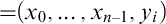
 $\{ x_0, \ldots , x_{n-1}, y_0, \ldots , y_{n-1}\}$
. We are interested in ensembles of such events, which allow non-deterministic and probabilistic variation in the outcomes of given measurements to be captured. Operationally, such ensembles can be generated by repeatedly performing multipartite measurements, and recording the outcomes. On the quantitative level, this will generate statistics, which can be represented by probability distributions on these events. We will look at this quantitative level later in the article, but for now, we focus on qualitative information at the possibilistic level: do certain outcomes for given measurements ever arise? This information can be represented by the set of possible assignments, which will have the following form:
$\{ x_0, \ldots , x_{n-1}, y_0, \ldots , y_{n-1}\}$
. We are interested in ensembles of such events, which allow non-deterministic and probabilistic variation in the outcomes of given measurements to be captured. Operationally, such ensembles can be generated by repeatedly performing multipartite measurements, and recording the outcomes. On the quantitative level, this will generate statistics, which can be represented by probability distributions on these events. We will look at this quantitative level later in the article, but for now, we focus on qualitative information at the possibilistic level: do certain outcomes for given measurements ever arise? This information can be represented by the set of possible assignments, which will have the following form:

We can think of X as a team (in the sense of team semantics) consisting of assignments of values to the variables
 $x_0,\dots ,x_{n-1},y_0,\dots ,y_{n-1}$
. Even though the data in its intended interpretation has a clear structure dividing the elements of the table into “inputs” and “outputs”, we can also look at the table as a mere database of data irrespective of how it was created. We can ask what kind of dependencies this table of data—team—manifests.
$x_0,\dots ,x_{n-1},y_0,\dots ,y_{n-1}$
. Even though the data in its intended interpretation has a clear structure dividing the elements of the table into “inputs” and “outputs”, we can also look at the table as a mere database of data irrespective of how it was created. We can ask what kind of dependencies this table of data—team—manifests.
Thus we can say that the team of data X supports strong determinism if it satisfies
 $$\begin{align*}\mathop{=}\hspace{-0.7pt}(x_i,y_i) \end{align*}$$
for all
 $i<n$
. Intuitively, in each such experiment, the input for the i
th party completely determines the outcome for that party, that is, the i
th outcome does not, in the light of X, depend on anything other than the i
th input. This is a very strong constraint, which limits the applicability of this concept.
$i<n$
. Intuitively, in each such experiment, the input for the i
th party completely determines the outcome for that party, that is, the i
th outcome does not, in the light of X, depend on anything other than the i
th input. This is a very strong constraint, which limits the applicability of this concept.
We say that the team X supports weak determinism if it satisfies
 $$\begin{align*}\mathop{=}\hspace{-0.7pt}(x_0,\ldots,x_{n-1},y_i) \end{align*}$$
for all
 $i<n$
. Intuitively, that says that the whole set of inputs to the system collectively completely determines each outcome, that is, the outcome does not, in the light of X, depend on anything else than the inputs of the system. In systems arising from scientific experiments, this means that the system has enough “variables” to determine its outcome.
$i<n$
. Intuitively, that says that the whole set of inputs to the system collectively completely determines each outcome, that is, the outcome does not, in the light of X, depend on anything else than the inputs of the system. In systems arising from scientific experiments, this means that the system has enough “variables” to determine its outcome.
Consider the Stern–Gerlach experiment. Even if the magnets are directed in the same way, the particles that pass through the magnetic field manifest a (quantized) spectrum of results, rather than a single spot on the receiving screen. In keeping with a fundamental tenet of quantum physics, all phenomena, such as tested by the Stern–Gerlach experiment, give only probabilistic results. An individual team may not reveal this, but the bigger the team, the more likely it is to fail to support even weak determinism.
There are important aspects of experimental data that cannot be expressed in terms of the dependence atom only. We therefore move on to a stronger concept, one that supersedes dependence and allows to express also independence.
In independence logic [Reference Grädel and Väänänen20], we add a new atomic formula
 $$\begin{align*}\vec{y}\perp_{\vec{x}}\vec{z} \end{align*}$$
to first-order logic. Intuitively this formula says that keeping
 $\vec {x}$
fixed,
$\vec {x}$
fixed,
 $\vec {y}$
and
$\vec {y}$
and
 $\vec {z}$
are independent of each other. A team X is defined to satisfy
$\vec {z}$
are independent of each other. A team X is defined to satisfy
 $\vec {y}\perp _{\vec {x}}\vec {z}$
if
$\vec {y}\perp _{\vec {x}}\vec {z}$
if
 $$ \begin{align*} &\qquad \forall s,s'\in X[s(\vec{x})=s'(\vec{x})\implies \\ \exists s"\in X &(s"(\vec{x})=s(\vec{x})\wedge s"(\vec{y})=s(\vec{y})\wedge s"(\vec{z})=s'(\vec{z})]. \end{align*} $$
We may observe that, unlike
 $\mathop {=}\hspace {-0.7pt}(x_0,\dots ,x_{n-1},y_i)$
, this is not closed downwardsFootnote
1
, but it is closed under unions of increasing chains. Note that this condition is first order, as was the case for the semantics of the dependence atom. Thus independence logic is
$\mathop {=}\hspace {-0.7pt}(x_0,\dots ,x_{n-1},y_i)$
, this is not closed downwardsFootnote
1
, but it is closed under unions of increasing chains. Note that this condition is first order, as was the case for the semantics of the dependence atom. Thus independence logic is
 $\Sigma ^1_1$
in its expressive power, and hence NP. Here is an example of a team satisfying
$\Sigma ^1_1$
in its expressive power, and hence NP. Here is an example of a team satisfying
 $y_0 \perp _{x_0x_1} y_1$
:
$y_0 \perp _{x_0x_1} y_1$
:

For fixed
 $x_0$
and
$x_0$
and
 $x_1$
, e.g.,
$x_1$
, e.g.,
 $x_0=0, x_1=1$
, the values of
$x_0=0, x_1=1$
, the values of
 $y_0$
and
$y_0$
and
 $y_1$
are independent of each other in the strong sense that if a value of
$y_1$
are independent of each other in the strong sense that if a value of
 $y_0$
occurs in combination with any value of
$y_0$
occurs in combination with any value of
 $y_1$
, e.g., 2, it occurs also with any other value of
$y_1$
, e.g., 2, it occurs also with any other value of
 $y_1$
, e.g., 7. Intuitively this says that in these experiments, the individual experiments do not interfere with each other. It is like measuring commuting quantum observables.
$y_1$
, e.g., 7. Intuitively this says that in these experiments, the individual experiments do not interfere with each other. It is like measuring commuting quantum observables.
Note that the dependence atom can be defined in terms of the independence atom:
 $$\begin{align*}\mathop{=}\hspace{-0.7pt}(\vec{x},\vec{y}) \equiv \vec{y} \perp_{\vec{x}} \vec{y}. \end{align*}$$
We will thus use
 $\mathop {=}\hspace {-0.7pt}(\vec {x},\vec {y})$
as a shorthand for
$\mathop {=}\hspace {-0.7pt}(\vec {x},\vec {y})$
as a shorthand for
 $\vec {y} \perp _{\vec {x}} \vec {y}$
when dealing with independence logic.
$\vec {y} \perp _{\vec {x}} \vec {y}$
when dealing with independence logic.
2.1 Syntax and semantics of independence logic
To rigorously define the semantics of independence logic—an extension of first-order logic by the independence atom—we need to be more precise about our definitions. For the sake of some technical details later on, we consider team semantics in the context of many-sorted structures (see, e.g., [Reference Manzano, Aranda, Zalta and Nodelman38]).
Definition 2.1. A (many-sorted relational) vocabulary
 $\tau $
is a tuple
$\tau $
is a tuple
 $(\mathrm {sor}_\tau ,\mathrm {rel}_\tau ,{\mathfrak {a}}_\tau ,{\mathfrak {s}}_\tau )$
such that
$(\mathrm {sor}_\tau ,\mathrm {rel}_\tau ,{\mathfrak {a}}_\tau ,{\mathfrak {s}}_\tau )$
such that
-
(i)
 $\mathrm {rel}_\tau $
is a set of relation symbolsFootnote
2
and
$\mathrm {sor}_\tau \subseteq \mathbb {N}$
,
$\mathrm {rel}_\tau $
is a set of relation symbolsFootnote
2
and
$\mathrm {sor}_\tau \subseteq \mathbb {N}$
, -
(ii)
${\mathfrak {a}}_\tau \colon \mathrm {rel}_\tau \to \mathbb {N}$
and
${\mathfrak {s}}_\tau \colon \mathrm {rel}_\tau \to \mathbb {N}^{<\omega }$
are functions with
${\mathfrak {s}}_\tau (R)\in \mathrm {sor}_\tau ^{{\mathfrak {a}}_\tau (R)}$
for
$R\in \mathrm {rel}_\tau $
, and -
(iii) if
$n_i\in \mathbb {N}$
,
$i<k$
, are such that
${\mathfrak {s}}_\tau (R)=(n_0,\dots ,n_{k-1})$
for some
${R\in \mathrm {rel}_\tau }$
, then
$n_0,\dots ,n_{k-1}\in \mathrm {sor}_\tau $
.


We call
 ${\mathfrak {a}}_\tau (R)$
the arity of R and
${\mathfrak {a}}_\tau (R)$
the arity of R and
 ${\mathfrak {s}}_\tau (R)$
the sort of R. For
${\mathfrak {s}}_\tau (R)$
the sort of R. For
 $n\notin \mathrm {sor}_\tau $
, we say that a vocabulary
$n\notin \mathrm {sor}_\tau $
, we say that a vocabulary
 $\tau '$
is the expansion of
$\tau '$
is the expansion of
 $\tau $
by the sort n if
$\tau $
by the sort n if
 $$\begin{align*}\tau'=(\mathrm{sor}_\tau\cup\{n\},\mathrm{rel}_\tau,{\mathfrak{s}}_\tau,{\mathfrak{a}}_\tau). \end{align*}$$
A (many-sorted)
 $\tau $
-structure is a function
$\tau $
-structure is a function
 $\mathfrak {A}$
defined on the set
$\mathfrak {A}$
defined on the set
 $\mathrm {rel}_\tau \cup \mathrm {sor}_\tau $
such that
$\mathrm {rel}_\tau \cup \mathrm {sor}_\tau $
such that
-
(i)
$\mathfrak {A}(n)$
is a nonempty set
$A_n$
for
$n\in \mathrm {sor}_\tau $
and called the sort n domain of
$\mathfrak {A}$
, and -
(ii)
$\mathfrak {A}(R)\subseteq A_{n_0}\times \dots \times A_{n_{k-1}}$
for
$R\in \mathrm {rel}_\tau $
, where
${\mathfrak {s}}_\tau (R)=(n_0,\dots ,n_{k-1})$
.


If
 $\tau '$
is an expansion of
$\tau '$
is an expansion of
 $\tau $
by sort n, we call a
$\tau $
by sort n, we call a
 $\tau '$
-structure
$\tau '$
-structure
 $\mathfrak {B}$
an expansion of
$\mathfrak {B}$
an expansion of
 $\mathfrak {A}$
by the sort n when
$\mathfrak {A}$
by the sort n when
 $\mathfrak {B}\restriction (\mathrm {rel}_\tau \cup \mathrm {sor}_\tau )=\mathfrak {A}$
.
$\mathfrak {B}\restriction (\mathrm {rel}_\tau \cup \mathrm {sor}_\tau )=\mathfrak {A}$
.
We usually denote
 $\mathfrak {A}(R)$
simply by
$\mathfrak {A}(R)$
simply by
 $R^{\mathfrak {A}}$
and
$R^{\mathfrak {A}}$
and
 $\mathfrak {A}(n)$
by
$\mathfrak {A}(n)$
by
 $A_n$
. If
$A_n$
. If
 $\mathfrak {A}$
only has one sort, then we denote the domain of that sort by A and call it the domain of
$\mathfrak {A}$
only has one sort, then we denote the domain of that sort by A and call it the domain of
 $\mathfrak {A}$
. When there is no risk for confusion, we write
$\mathfrak {A}$
. When there is no risk for confusion, we write
 ${\mathfrak {a}}$
and
${\mathfrak {a}}$
and
 ${\mathfrak {s}}$
for
${\mathfrak {s}}$
for
 ${\mathfrak {a}}_\tau $
and
${\mathfrak {a}}_\tau $
and
 ${\mathfrak {s}}_\tau $
.
${\mathfrak {s}}_\tau $
.
For each sort
 $n\in \mathbb {N}$
, we designate a set
$n\in \mathbb {N}$
, we designate a set
 $\{v_i^n \mid i\in \mathbb {N}\}$
of variables of sort n, although for simplicity of notation, we usually use symbols like x,
$\{v_i^n \mid i\in \mathbb {N}\}$
of variables of sort n, although for simplicity of notation, we usually use symbols like x,
 $y,$
and z for variables and indicate the sort by writing
$y,$
and z for variables and indicate the sort by writing
 ${\mathfrak {s}}(x)$
for the sort of x.
${\mathfrak {s}}(x)$
for the sort of x.
Definition 2.2 (Syntax of Independence Logic)
The set of
 $\tau $
-formulas of independence logic is defined as follows.
$\tau $
-formulas of independence logic is defined as follows.
-
(i) First-order atomic and negated atomic formulas
$u=v$
,
$\neg u=v$
,
$R(\vec {x})$
and
$\neg R(\vec {x})$
, where
$R\in \mathrm {rel}_\tau $
,
$\vec {x}=(x_0,\dots ,x_{{\mathfrak {a}}(R)-1})$
and
$v$
,
$u,$
and
$x_i$
are variables with
${\mathfrak {s}}(u),{\mathfrak {s}}(v),{\mathfrak {s}}(x_i)\in \mathrm {sor}_\tau $
,
${\mathfrak {s}}(u)={\mathfrak {s}}(v)$
Footnote
3
and
${\mathfrak {s}}(R)=({\mathfrak {s}}(x_0),\dots ,{\mathfrak {s}}(x_{{\mathfrak {a}}(R)-1}))$
, are
$\tau $
-formulas. -
(ii) Independence atoms
$\vec {y}\perp _{\vec {x}}\vec {z}$
, where
$\vec {x}=(x_0,\dots ,x_{n-1})$
,
$\vec {y}=(y_0,\dots ,y_{m-1})$
, and
$\vec {z}=(z_0,\dots ,z_{l-1})$
, and
$x_i$
,
$y_j$
, and
$z_k$
are variables with
${\mathfrak {s}}(x_i),{\mathfrak {s}}(y_j),{\mathfrak {s}}(z_k)\in \mathrm {sor}_\tau $
, are
$\tau $
-formulas. -
(iii) If
$\varphi $
and
$\psi $
are
$\tau $
-formulas, then so are
$\varphi \land \psi $
and
$\varphi \lor \psi $
. -
(iv) If
$\varphi $
is a
$\tau $
-formula and
$v$
is a variable with
${\mathfrak {s}}(v)\in \mathrm {sor}_\tau $
, then also
$\forall v\varphi $
and
$\exists v\varphi $
are
$\tau $
-formulas.


We call dependence logic the fragment of independence logic where only independence atoms of the form
 $\vec {y}\perp _{\vec {x}}\vec {y}$
are allowed.
$\vec {y}\perp _{\vec {x}}\vec {y}$
are allowed.
In addition to the usual syntax of independence logic, we introduce new quantifiers
 $\tilde {\forall }$
and
$\tilde {\forall }$
and
 $\tilde {\exists }$
which we will interpret as new sort quantifiers. Similar quantifiers—although second order—were introduced by the third author in [Reference Väänänen46].
$\tilde {\exists }$
which we will interpret as new sort quantifiers. Similar quantifiers—although second order—were introduced by the third author in [Reference Väänänen46].
-
(v) If
$v$
is a variable such that
${\mathfrak {s}}(v)\notin \mathrm {sor}_\tau $
,
$\tau '$
is the expansion of
$\tau $
by the sort
${\mathfrak {s}}(v)$
and
$\varphi $
is a
$\tau '$
-formula such that no variable, other than
$v$
, of sort
${\mathfrak {s}}(v)$
occurs free in
$\varphi $
, then
$\tilde {\forall }v\varphi $
and
$\tilde {\exists }v\varphi $
are
$\tau $
-formulas.


The underlying idea of the new sort quantifiers
 $\tilde {\exists }$
and
$\tilde {\exists }$
and
 $\tilde {\forall }$
will become apparent in Definition 2.4 below.
$\tilde {\forall }$
will become apparent in Definition 2.4 below.
Definition 2.3. Let
 $\mathfrak {A}$
be a
$\mathfrak {A}$
be a
 $\tau $
-structure and D a set of variables. An assignment s of
$\tau $
-structure and D a set of variables. An assignment s of
 $\mathfrak {A}$
with domain D is a function
$\mathfrak {A}$
with domain D is a function
 $D\to \bigcup _{n\in \mathrm {sor}_\tau }A_n$
such that
$D\to \bigcup _{n\in \mathrm {sor}_\tau }A_n$
such that
 $s(v)\in A_{{\mathfrak {s}}(v)}$
for all
$s(v)\in A_{{\mathfrak {s}}(v)}$
for all
 $v\in D$
. If s is an assignment of
$v\in D$
. If s is an assignment of
 $\mathfrak {A}$
with domain D, we write
$\mathfrak {A}$
with domain D, we write
 $s\colon D\to \mathfrak {A}$
. A team X of
$s\colon D\to \mathfrak {A}$
. A team X of
 $\mathfrak {A}$
with domain D is a set of assignments of
$\mathfrak {A}$
with domain D is a set of assignments of
 $\mathfrak {A}$
with domain D. We denote by
$\mathfrak {A}$
with domain D. We denote by
 $\operatorname {\mathrm {dom}}(X)$
the set D and by
$\operatorname {\mathrm {dom}}(X)$
the set D and by
 $\operatorname {\mathrm {rng}}(X)$
the set
$\operatorname {\mathrm {rng}}(X)$
the set
 $\{s(v) \mid v\in D, s\in X\}$
. If X contains every assignment of
$\{s(v) \mid v\in D, s\in X\}$
. If X contains every assignment of
 $\mathfrak {A}$
, we call X the full team of
$\mathfrak {A}$
, we call X the full team of
 $\mathfrak {A}$
.
$\mathfrak {A}$
.
For an assignment
 $s\colon D\to \mathfrak {A}$
, a variable
$s\colon D\to \mathfrak {A}$
, a variable
 $v$
(not necessarily in D) and
$v$
(not necessarily in D) and
 $a\in A_{{\mathfrak {s}}(v)}$
, we denote by
$a\in A_{{\mathfrak {s}}(v)}$
, we denote by
 $s(a/v)$
the assignment
$s(a/v)$
the assignment
 $D\cup \{v\}\to \mathfrak {A}$
that maps
$D\cup \{v\}\to \mathfrak {A}$
that maps
 $v$
to a and
$v$
to a and
 $w$
to
$w$
to
 $s(w)$
for
$s(w)$
for
 $w\in D\setminus \{v\}$
. If
$w\in D\setminus \{v\}$
. If
 $\vec {x}=(x_0,\dots ,x_{n-1})$
is a tuple of variables, we denote by
$\vec {x}=(x_0,\dots ,x_{n-1})$
is a tuple of variables, we denote by
 $s(\vec {x})$
the tuple
$s(\vec {x})$
the tuple
 $(s(x_0),\dots ,s(x_{n-1}))$
.
$(s(x_0),\dots ,s(x_{n-1}))$
.
Given a team X of
 $\mathfrak {A}$
, a variable
$\mathfrak {A}$
, a variable
 $v$
, and a function
$v$
, and a function
 $F\colon X\to {\mathcal {P}}(A_{{\mathfrak {s}}(v)})\setminus \{\emptyset \}$
, we denote by
$F\colon X\to {\mathcal {P}}(A_{{\mathfrak {s}}(v)})\setminus \{\emptyset \}$
, we denote by
 $X[F/v]$
the (“supplemented”) team
$X[F/v]$
the (“supplemented”) team
 $\{s(a/v) \mid s\in X, a\in F(s)\}$
and by
$\{s(a/v) \mid s\in X, a\in F(s)\}$
and by
 $X[A_{{\mathfrak {s}}(v)}/v]$
the (“duplicated”) team
$X[A_{{\mathfrak {s}}(v)}/v]$
the (“duplicated”) team
 $\{s(a/v) \mid s\in X, a\in A_{{\mathfrak {s}}(v)}\}$
.
$\{s(a/v) \mid s\in X, a\in A_{{\mathfrak {s}}(v)}\}$
.
Definition 2.4 (Semantics of Independence Logic)
Let
 $\tau $
be a (possibly many-sorted) vocabulary,
$\tau $
be a (possibly many-sorted) vocabulary,
 $\mathfrak {A}$
a
$\mathfrak {A}$
a
 $\tau $
-structure, X a team of
$\tau $
-structure, X a team of
 $\mathfrak {A}$
, and
$\mathfrak {A}$
, and
 $\varphi $
a
$\varphi $
a
 $\tau $
-formula. We then define the concept of the team X satisfying the formula
$\tau $
-formula. We then define the concept of the team X satisfying the formula
 $\varphi $
in the structure
$\varphi $
in the structure
 $\mathfrak {A}$
, in symbols
$\mathfrak {A}$
, in symbols
 $\mathfrak {A}\models _X\varphi $
, as follows.Footnote
4
$\mathfrak {A}\models _X\varphi $
, as follows.Footnote
4
-
(i) If
$\varphi $
is a first-order atomic or negated atomic formula, then
$\mathfrak {A}\models _X\varphi $
if every assignment
$s\in X$
satisfies
$\varphi $
in
$\mathfrak {A}$
in the usual sense. -
(ii) If
$\varphi = \vec {y}\perp _{\vec {x}}\vec {z}$
, then
$\mathfrak {A}\models _X\varphi $
if for any
$s,s'\in X$
with
$s(\vec {x})=s'(\vec {x})$
there exists
$s"\in X$
with
$s"(\vec {x}\vec {y})=s(\vec {x}\vec {y})$
and
$s"(\vec {z})=s'(\vec {z})$
. -
(iii) If
$\varphi =\psi \land \theta $
, then
$\mathfrak {A}\models _X\varphi $
if
$\mathfrak {A}\models _X\psi $
and
$\mathfrak {A}\models _X\theta $
. -
(iv) If
$\varphi =\psi \lor \theta $
, then
$\mathfrak {A}\models _X\varphi $
if
$\mathfrak {A}\models _Y\psi $
and
$\mathfrak {A}\models _Z\theta $
for some teams Y and Z such that
$Y\cup Z = X$
. -
(v) If
$\varphi =\forall v\psi $
, then
$\mathfrak {A}\models _X\varphi $
if
$\mathfrak {A}\models _{X[A_{{\mathfrak {s}}(v)}/v]}\psi $
. -
(vi) If
$\varphi =\exists v\psi $
, then
$\mathfrak {A}\models _X\varphi $
if
$\mathfrak {A}\models _{X[F/v]}\psi $
for some function
$F\colon X\to {\mathcal {P}}(A_{{\mathfrak {s}}(v)})\setminus \{\emptyset \}$
. -
(vii) If
$\varphi =\tilde {\forall }v\psi $
, then
$\mathfrak {A}\models _X\varphi $
if
$\mathfrak {B}\models _X\forall v\psi $
for all expansions
$\mathfrak {B}$
of
$\mathfrak {A}$
by the sort
${{\mathfrak {s}}(v)}$
. -
(viii) If
$\varphi =\tilde {\exists }v\psi $
, then
$\mathfrak {A}\models _X\varphi $
if
$\mathfrak {B}\models _X\exists v\psi $
for some expansion
$\mathfrak {B}$
of
$\mathfrak {A}$
by the sort
${{\mathfrak {s}}(v)}$
.


If we restrict our attention to vocabularies and structures with just one sort, we get exactly the ordinary team semantics of independence logic.
When the underlying structure
 $\mathfrak {A}$
is clear from the context or is irrelevant to the discussion (e.g., when the formula
$\mathfrak {A}$
is clear from the context or is irrelevant to the discussion (e.g., when the formula
 $\varphi $
does not contain any non-logical symbols or variables of multiple sorts), we simply write
$\varphi $
does not contain any non-logical symbols or variables of multiple sorts), we simply write
 $X\models \varphi $
instead of
$X\models \varphi $
instead of
 $\mathfrak {A}\models _X\varphi $
.
$\mathfrak {A}\models _X\varphi $
.
2.2 Axioms of independence logic
Although logical consequences in team semantics cannot be completely axiomatized (see the beginning of Section 3.4), it makes sense to isolate axioms that suffice for proving as many of the interesting logical consequences as possible. The rules we present here are, of course, not intended to be complete in any sense; rather, they are just what we need in this article. The general question of a more complete set of rules and axioms remains open.
Definition 2.5 (Axioms of the Independence Atom, [Reference Galliani and Väänänen17, Reference Grädel and Väänänen20])
The axioms of the independence atom are:
-
(i)
$\vec {y}\perp _{\vec {x}}\vec {y}$
entails
$\vec {y}\perp _{\vec {x}}\vec {z}$
. (Constancy Rule) -
(ii)
$\vec {x}\perp _{\vec {x}}\vec {y}$
. (Reflexivity Rule) -
(iii)
$\vec {z}\perp _{\vec {x}}\vec {y}$
entails
$\vec {y}\perp _{\vec {x}}\vec {z}$
. (Symmetry Rule) -
(iv)
$\vec {y}{y'}\perp _{\vec {x}}\vec {z}{z'}$
entails
$\vec {y}\perp _{\vec {x}}\vec {z}$
. (Weakening Rule) -
(v) If
$\vec {z'}$
is a permutation of
$\vec {z}$
,
$\vec {x'}$
is a permutation of
$\vec {x}$
,
$\vec {y'}$
is a permutation of
$\vec {y}$
, then
$\vec {y}\perp _{\vec {x}}\vec {z}$
entails
$\vec {y'}\perp _{\vec {x'}}\vec {z'}$
. (Permutation Rule) -
(vi)
$\vec {z}\perp _{\vec {x}}\vec {y}$
entails
$\vec {y}\vec {x}\perp _{\vec {x}}\vec {z}\vec {x}$
. (Fixed Parameter Rule) -
(vii)
$\vec {x}\perp _{\vec {z}}\vec {y}\wedge \vec {u}\perp _{\vec {z}\vec {x}}\vec {y}$
entails
$\vec {u}\perp _{\vec {z}}\vec {y}$
. (First Transitivity Rule) -
(viii)
$\vec {y}\perp _{\vec {z}}\vec {y}\wedge \vec {z}\vec {x}\perp _{\vec {y}}\vec {u}$
entails
$\vec {x}\perp _{\vec {z}}\vec {u}$
. (Second Transitivity Rule) -
(ix)
$\vec {x}\perp _{\vec {z}}\vec {y}\land \vec {x}\vec {y}\perp _{\vec {z}}\vec {u}$
entails
$\vec {x}\perp _{\vec {z}}\vec {y}\vec {u}$
. (Exchange Rule)


The so-called Armstrong’s Axioms for the dependence atom [Reference Armstrong and Rosenfeld7] follow from the above axioms.
Definition 2.6 (Axioms of Dependence Atom)
The axioms of the dependence atom are:
-
(i)
$\mathop {=}\hspace {-0.7pt}({\vec {x}}{\vec {y}},{\vec {x}})$
. (Reflexivity) -
(ii)
$\mathop {=}\hspace {-0.7pt}({\vec {x}},{\vec {y}})\land \mathop {=}\hspace {-0.7pt}({\vec {y}},{\vec {z}})$
entails
$\mathop {=}\hspace {-0.7pt}({\vec {x}},{\vec {z}})$
. (Transitivity) -
(iii)
$\mathop {=}\hspace {-0.7pt}({\vec {x}},{\vec {y}})$
entails
$\mathop {=}\hspace {-0.7pt}({\vec {x}},{\vec {x}}{\vec {y}})$
. (Extensivity) -
(iv) If
$\vec {x'}$
and
$\vec {y'}$
are permutations of
${\vec {x}}$
and
${\vec {y}}$
, respectively, then
$\mathop {=}\hspace {-0.7pt}({\vec {x}},{\vec {y}})$
entails
$\mathop {=}\hspace {-0.7pt}(\vec {x'},\vec {y'})$
. (Permutation)


Armstrong’s axioms are complete for dependence atoms, i.e., if
 $\Sigma $
is a set of dependence atoms and
$\Sigma $
is a set of dependence atoms and
 $\varphi $
is another dependence atom, then
$\varphi $
is another dependence atom, then
 $\Sigma \models \varphi $
if and only if
$\Sigma \models \varphi $
if and only if
 $\Sigma $
entails
$\Sigma $
entails
 $\varphi $
by repeated applications of Armstrong’s axioms.
$\varphi $
by repeated applications of Armstrong’s axioms.
The notion of a graphoid was introduced in [Reference Pearl and Paz40] after the observation that certain axioms that hold true for conditional independence in probability theory are also satisfied by the vertex separation relation in a(n undirected) graph. A semigraphoid is a weakening of a graphoid, excluding one axiom. The axioms as we present them can be found in [Reference Pearl39].
Definition 2.7. The following are the semigraphoid axioms:
-
(S1)
$\vec x\perp _{\vec z}\emptyset $
. (Triviality) -
(S2)
$\vec {x}\perp _{\vec {z}}\vec {y}$
entails
$\vec {y}\perp _{\vec {z}}\vec {x}$
. (Symmetry) -
(S3)
$\vec x\perp _{\vec z}\vec y\vec w$
entails
$\vec x\perp _{\vec z}\vec y$
. (Decomposition) -
(S4)
$\vec x\perp _{\vec z}\vec y\vec w$
entails
$\vec x\perp _{\vec z\vec w}\vec y$
. (Weak Union) -
(S5)
$\vec {x}\perp _{\vec {z}}\vec {y} \land \vec {x}\perp _{\vec {z}\vec y}\vec {w}$
entails
$\vec {x}\perp _{\vec {z}}\vec {y}\vec w$
. (Contraction)


In the original definition of a (semi)graphoid,
 $\vec x$
,
$\vec x$
,
 $\vec y$
,
$\vec y$
,
 $\vec z,$
and
$\vec z,$
and
 $\vec w$
are sets instead of tuples, so we add the following (trivially valid) axioms to accommodate that:
$\vec w$
are sets instead of tuples, so we add the following (trivially valid) axioms to accommodate that:
-
(vi) If
$\vec {x'}$
,
$\vec {y'}$
, and
$\vec {z'}$
are permutations of
$\vec x$
,
$\vec y$
, and
$\vec {z}$
, respectively, then
$\vec {x}\perp _{\vec {z}}\vec {y}$
entails
$\vec {x'}\perp _{\vec {z'}}\vec {y'}$
. (Permutation) -
(vii)
$\vec {x}\perp _{\vec {z}}\vec {y}$
entails
$\vec {x}\vec x\perp _{\vec {z}\vec z}\vec {y}\vec y$
. (Repetition)


It is straightforward to show that the semigraphoid axioms are sound in team semantics (a fact which also follows from Proposition 4.23). Next we show that the axioms of independence atom follow from the semigraphoid axioms, save the Reflexivity Rule. It remains open whether the Reflexivity Rule also follows from the semigraphoid axioms.
Proposition 2.8. The axioms of the independence atom are provable from the semigraphoid axioms + the Reflexivity Rule.
Proof
-
(i) Constancy Rule: Reflexivity rule gives
$\vec x\vec y\perp _{\vec x\vec y}\vec z$
. By a combination of symmetry, permutation, and decomposition, from this, we get
$\vec y\perp _{\vec x\vec y}\vec z$
. From
$\vec y\perp _{\vec x}\vec y \land \vec y\perp _{\vec x\vec y}\vec z$
, contraction gives
$\vec y\perp _{\vec x}\vec y\vec z$
, whence by decomposition, we get
$\vec y\perp _{\vec x}\vec z$
. -
(ii) Reflexivity Rule: is an assumption.
-
(iii) Symmetry Rule: This is the same as the symmetry axiom of semigraphoids.
-
(iv) Weakening Rule: By the decomposition axiom,
$\vec {y}{y'}\perp _{\vec {x}}\vec {z}{z'}$
entails
$\vec {y}{y'}\perp _{\vec {x}}\vec {z}$
, which by symmetry entails
$\vec {z}\perp _{\vec {x}}\vec {y}{y'}$
, which by decomposition entails
$\vec {z}\perp _{\vec {x}}\vec {y}$
, which by symmetry gives
$\vec {y}\perp _{\vec {x}}\vec {z}$
. -
(v) Permutation Rule: This is the same as permutation of semigraphoids.
-
(vi) Fixed Parameter Rule: From the Reflexivity Rule and symmetry, we get
$\vec y\perp _{\vec x}\vec x$
. From
$\vec y\perp _{\vec x}\vec z$
, we get
$\vec y\perp _{\vec x\vec x}\vec z$
by repetition. From
$\vec y\perp _{\vec x}\vec x \land \vec y\perp _{\vec x\vec x}\vec z$
, contraction gives
$\vec y\perp _{\vec x}\vec x\vec z$
. By symmetry and repetition, we have
$\vec x\vec z\perp _{\vec x\vec x}\vec y$
, and again reflexivity + symmetry gives
$\vec x\vec z\perp _{\vec x}\vec x$
. From
$\vec x\vec z\perp _{\vec x}\vec x \land \vec x\vec z\perp _{\vec x\vec x}\vec y$
, contraction again gives
$\vec x\vec z\perp _{\vec x}\vec x\vec y$
. By symmetry + permutation, this yields
$\vec y\vec x\perp _{\vec x}\vec z\vec x$
as desired. -
(vii) First Transitivity Rule: By symmetry, from
$\vec {x}\perp _{\vec {z}}\vec {y}$
, we get
$\vec {y}\perp _{\vec {z}}\vec {x}$
and from
$\vec {u}\perp _{\vec {z}\vec {x}}\vec {y}$
, we get
$\vec {y}\perp _{\vec {z}\vec {x}}\vec {u}$
. Applying contraction to
$\vec {y}\perp _{\vec {z}}\vec {x}$
and
$\vec {y}\perp _{\vec {z}\vec {x}}\vec {u}$
, we get
$\vec {y}\perp _{\vec {z}}\vec {x}\vec {u}$
, from which the weakening rule that we already proved gives
$\vec {y}\perp _{\vec {z}}\vec {u}$
. Then, by symmetry, we get
$\vec {u}\perp _{\vec {z}}\vec {y}$
. -
(viii) Second Transitivity Rule: From
$\vec {z}\vec {x}\perp _{\vec {y}}\vec {u}$
, symmetry, permutation, and weak union give
$\vec {x}\perp _{\vec {z}\vec {y}}\vec {u}$
. From
$\vec y\perp _{\vec z}\vec y$
, constancy rule + symmetry gives
$\vec x\perp _{\vec z}\vec y$
. Then contraction gives
$\vec x\perp _{\vec z}\vec y\vec u$
, whence by decomposition, we obtain
$\vec x\perp _{\vec z}\vec u$
. -
(ix) Exchange Rule: From
$\vec {x}\vec {y}\perp _{\vec {z}}\vec {u}$
, symmetry + weak union gives
$\vec {x}\perp _{\vec {z}\vec {y}}\vec {u}$
. Then from
$\vec {x}\perp _{\vec {z}}\vec {y}$
and
$\vec {x}\perp _{\vec {z}\vec {y}}\vec {u}$
, contraction gives
$\vec {x}\perp _{\vec {z}}\vec {y}\vec {u}$
.


So it turns out that the semigraphoid axioms, with the Reflexivity Rule added, are sufficient to prove all the others. This will be useful in Section 4. However, we will use all of the above axioms in the sequel.
Next we add rules for conjunction and existential quantifier, as we shall be working mainly with an existential-conjunctive fragment of independence logic.
Definition 2.9 (Quantifiers and Connectives, [Reference Hannula23, Reference Kontinen and Väänänen35])
-
(i) The following is the elimination rule for existential quantifier:
If
$\Sigma $
is a set of formulas,
$\Sigma \cup \{\varphi \}$
entails
$\psi $
and x does not occur free in
$\psi $
or in any
$\theta \in \Sigma $
, then
$\Sigma \cup \{\exists x\varphi \}$
entails
$\psi $
. -
(ii) The following is the introduction rule for existential quantifier:
If y does not occur in the scope of
$Qx$
in
$\varphi $
for any
${Q\in \{\exists ,\forall ,\tilde {\exists },\tilde {\forall }\}}$
, then
$\varphi (y/x)$
(i.e., the formula one obtains by replacing every free occurrence of x in
$\varphi $
by y) entails
$\exists x\varphi $
. -
(iii) The following is the elimination rule for conjunction:
$\varphi \land \psi $
entails both
$\varphi $
and
$\psi $
. -
(iv) The following is the introduction rule for conjunction:
$\{\varphi ,\psi \}$
entails
$\varphi \land \psi $
. -
(v) The following is the rule for dependence introduction:
$\exists x\varphi $
entails
$\exists x (\mathop {=}\hspace {-0.7pt}(\vec {z},x)\land \varphi )$
whenever
$\varphi $
is a formula of dependence logic, where
$\vec {z}$
lists the free variables of
$\exists x\varphi $
. -
(vi) The following is the first introduction rule for
$\tilde \exists $
:If no variable with sort
${\mathfrak {s}}(x)$
occurs in any formula of
$\Sigma $
and
$\Sigma $
entails
$\exists x\varphi $
, then
$\Sigma $
entails
$\tilde \exists x\varphi $
. -
(vii) The following is the second introduction rule for
$\tilde \exists $
:If no variable with sort
${\mathfrak {s}}(x)$
occurs in any formula of
$\Sigma $
and
$\Sigma \cup \{\exists x\varphi \}$
entails
$\exists y\psi $
, where
${\mathfrak {s}}(y) = {\mathfrak {s}}(x)$
, then
$\Sigma \cup \{\tilde \exists x\varphi \}$
entails
$\tilde \exists y\psi $
.


For the new sort existential quantifier
 $\tilde \exists $
, we only give the above rather immediate axioms. These rules could possibly be strengthened by allowing variables of sort
$\tilde \exists $
, we only give the above rather immediate axioms. These rules could possibly be strengthened by allowing variables of sort
 ${\mathfrak {s}}(x)$
occur in the scope of
${\mathfrak {s}}(x)$
occur in the scope of
 $\tilde \exists y$
for
$\tilde \exists y$
for
 ${\mathfrak {s}}(y) = {\mathfrak {s}}(x)$
in formulas of
${\mathfrak {s}}(y) = {\mathfrak {s}}(x)$
in formulas of
 $\Sigma $
. It may also be interesting to look for more axioms for the sort quantifiers. For example,
$\Sigma $
. It may also be interesting to look for more axioms for the sort quantifiers. For example,
 $\tilde \exists x\exists y \neg x=y$
for
$\tilde \exists x\exists y \neg x=y$
for
 ${\mathfrak {s}}(x)={\mathfrak {s}}(y)$
is a natural valid sentence (even though the sentence
${\mathfrak {s}}(x)={\mathfrak {s}}(y)$
is a natural valid sentence (even though the sentence
 $\exists x\exists y \neg x=y$
is not valid) but apparently not derivable from our current axioms.
$\exists x\exists y \neg x=y$
is not valid) but apparently not derivable from our current axioms.
Proposition 2.10 (Soundness Theorem)
If
 $\varphi $
entails
$\varphi $
entails
 $\psi $
by repeated applications of the rules of Definitions 2.5–2.9, then
$\psi $
by repeated applications of the rules of Definitions 2.5–2.9, then
 $\varphi \models \psi $
in team semantics.
$\varphi \models \psi $
in team semantics.
Proof We show that the rules for
 $\tilde \exists $
are sound. For the second introduction rule, suppose that
$\tilde \exists $
are sound. For the second introduction rule, suppose that
 $\Sigma \cup \{\exists x\varphi \}\models \exists y\psi $
, where
$\Sigma \cup \{\exists x\varphi \}\models \exists y\psi $
, where
 ${\mathfrak {s}}(y) = {\mathfrak {s}}(x)$
. Then suppose that
${\mathfrak {s}}(y) = {\mathfrak {s}}(x)$
. Then suppose that
 $\mathfrak {A}\models _X\Sigma \cup \{\tilde \exists x\varphi \}$
. Then
$\mathfrak {A}\models _X\Sigma \cup \{\tilde \exists x\varphi \}$
. Then
 $\mathfrak {A}$
has an expansion
$\mathfrak {A}$
has an expansion
 $\mathfrak {A}^{*}$
by the sort
$\mathfrak {A}^{*}$
by the sort
 ${\mathfrak {s}}(x)$
with
${\mathfrak {s}}(x)$
with
 $\mathfrak {A}^{*}\models _X\Sigma \cup \{\exists x\varphi \}$
. Thus
$\mathfrak {A}^{*}\models _X\Sigma \cup \{\exists x\varphi \}$
. Thus
 $\mathfrak {A}^{*}\models _X\exists y\psi $
, whence
$\mathfrak {A}^{*}\models _X\exists y\psi $
, whence
 $\mathfrak {A}\models _X\tilde \exists y\psi $
. The first introduction rule is the same but without the assumption
$\mathfrak {A}\models _X\tilde \exists y\psi $
. The first introduction rule is the same but without the assumption
 $\tilde \exists x\varphi $
.
$\tilde \exists x\varphi $
.
If
 $\varphi $
entails
$\varphi $
entails
 $\psi $
by repeated applications of the above rules, we write
$\psi $
by repeated applications of the above rules, we write
 $\varphi \vdash \psi $
.
$\varphi \vdash \psi $
.
3 Logical properties of teams
Quantum physics provides a rich source of highly non-trivial dependence and independence concepts. Some of the most fundamental questions of quantum physics concern independence of outcomes of experiments. The first author presented in [Reference Abramsky1] a relational (possibilistic) approach to model these dependence and independence phenomena. His framework very naturally transforms into a team-semantic adaptation which we will carry out now.
3.1 Empirical and hidden-variable teams
As discussed in Section 2, we consider teams with designated variables for measurements and separate variables for outcomes. An important role in models of quantum physics is played by the so-called hidden variables, variables which are not directly observable, but which play a role in determining the outcomes of measurements, explaining indeterministic or non-local behaviour. The following terminology and notation is helpful in dealing with teams arising in this way in relation to quantum physics.
We use a division of variables into three sorts, defined below. A priori, there is no difference between the variables. This division into three sorts is simply helpful in guiding our intuitions. Our purely abstract results about teams based on these variables help us organize quantum-theoretic concepts. However, it is worth noting that, e.g., the word “measurement” has a meaning that corresponds to a physical event and the assumptions we make in the form of the properties of teams presented in Section 3.2, of course reflect the properties—observed or postulated—of these physical events.
Definition 3.1. Fix
-
• a set
$V_{\text {m}} = \{x_0,\dots ,x_{n-1}\}$
of measurement variables, -
• a corresponding set
$V_{\text {o}} = \{y_0,\dots ,y_{n-1}\}$
of outcome variables, and -
• a set
$V_{\text {h}} = \{z_0,\dots ,z_{l-1}\}$
of hidden variables.
We say that a team X is an empirical team if
 $\operatorname {\mathrm {dom}}(X)=V_{\text {m}}\cup V_{\text {o}}$
. We say that a team X is a hidden-variable team if
$\operatorname {\mathrm {dom}}(X)=V_{\text {m}}\cup V_{\text {o}}$
. We say that a team X is a hidden-variable team if
 $\operatorname {\mathrm {dom}}(X)=V_{\text {m}}\cup V_{\text {o}}\cup V_{\text {h}}$
.
$\operatorname {\mathrm {dom}}(X)=V_{\text {m}}\cup V_{\text {o}}\cup V_{\text {h}}$
.
Throughout the article, we will denote by n the number of measurement and outcome variables and by l the number of hidden variables.
Definition 5.2 below makes the connection between our concept of an empirical team and the mathematical model predicting what the possible outcomes of experiments could be, namely, the theory of operators of complex Hilbert spaces, explicit.
We will pay special attention to definability of properties of teams. In other words, if P is a property of teams, especially of empirical or hidden-variable teams, we ask whether there is a formula
 $\varphi $
of independence logic with the free variables
$\varphi $
of independence logic with the free variables
 $V_{\text {m}}\cup V_{\text {o}}$
(or
$V_{\text {m}}\cup V_{\text {o}}$
(or
 $V_{\text {m}}\cup V_{\text {o}}\cup V_{\text {h}}$
) which is satisfied in the sense of team semantics exactly by those teams that have the property P.
$V_{\text {m}}\cup V_{\text {o}}\cup V_{\text {h}}$
) which is satisfied in the sense of team semantics exactly by those teams that have the property P.
A hidden-variable team is a team of the form

where the
 $\gamma ^i_j$
indicate values which we cannot observe directly. A typical hidden variable is some kind of “state” of the system.
$\gamma ^i_j$
indicate values which we cannot observe directly. A typical hidden variable is some kind of “state” of the system.
Every team has a background model from which the values of assignments come. In a many-sorted context, the background model has one universe for each sort. The universes may intersect. We assume a universe also for the hidden-variable sort.
Definition 3.2 [Reference Abramsky1]
A hidden-variable team Y realizes an empirical team X if
 $$\begin{align*}s\in X \iff \exists s'\in Y \bigwedge_{i<n}(s'(x_i)=s(x_i) \land s'(y_i)=s(y_i)). \end{align*}$$
Two hidden-variable teams are said to be (empirically) equivalent if they realize the same empirical team.
The property of being the realization of a hidden-variable team is definable in independence logic. It can be defined simply by the existential quantifier: If
 $\varphi (\vec {x},\vec {y},\vec {z})$
is a formula of independence logic, and thereby defines a property of teams, then
$\varphi (\vec {x},\vec {y},\vec {z})$
is a formula of independence logic, and thereby defines a property of teams, then
 $\tilde {\exists } z_0\exists z_1\dots \exists z_{l-1}\varphi $
defines the class of empirical teams that are realized by some hidden-variable teams satisfying
$\tilde {\exists } z_0\exists z_1\dots \exists z_{l-1}\varphi $
defines the class of empirical teams that are realized by some hidden-variable teams satisfying
 $\varphi $
. The “hidden” character of the hidden variables is built into the semantics of the sort quantifier.
$\varphi $
. The “hidden” character of the hidden variables is built into the semantics of the sort quantifier.
Realization of an empirical team by a hidden-variable team involves a kind of projection where one projects away the hidden variables. Hidden-variable teams are divided into equivalence classes according to whether they project into the same empirical team or not. This phenomenon can, of course, be thought of more generally: for any set V of variables and
 $V'\subseteq V$
, one can define a projection mapping
$V'\subseteq V$
, one can define a projection mapping
 $\Pr _{V'}$
such that if X is a team with domain V, then
$\Pr _{V'}$
such that if X is a team with domain V, then
 $\Pr _{V'}(X) = \{s\restriction V' \mid s\in X \}$
.
$\Pr _{V'}(X) = \{s\restriction V' \mid s\in X \}$
.
Next we use the resources of independence logic with its team semantics to express properties of empirical and hidden-variable teams. The possible benefits of expressing such properties in the formal language of independence logic are two-fold. First, the quantum-theoretic concepts may suggest interesting new facts about independence logic in general, applicable perhaps also in other fields. Second, concepts, proofs, and constructions of independence logic may shed new light on connections between concepts in quantum physics, and may focus attention on what is particular to quantum physics, and what are merely general logical facts about independence concepts.
3.2 Properties of empirical teams
We observe that the definitions of the simpler properties of empirical teams treated by the first author in [Reference Abramsky1] can be expressed by formulas of independence logic, in fact a conjunction of independence atoms. For the original definitions, we refer to [Reference Bell9, Reference Dickson13, Reference Jarrett32, Reference Shimony42].
As discussed in Section 2, a team is said to support weak determinism if each outcome is determined by the combination of all the measurement variables.
Definition 3.3 (Weak Determinism)
An empirical team X supports weak determinism if it satisfies the formula
 $$ \begin{align} \bigwedge_{i<n} \mathop{=}\hspace{-0.7pt}(\vec{x},y_i). \end{align} $$
Thus weak determinism is expressed simply with a conjunction of dependence atoms. In fact, the meaning of the dependence atom
 $\mathop {=}\hspace {-0.7pt}(x,y)$
is that x completely determines y. Therefore saying that teams supporting (WD) support weak determinism is appropriate. The only difference to the ordinary dependence atom is that in (WD) we separate the variables into the measurements
$\mathop {=}\hspace {-0.7pt}(x,y)$
is that x completely determines y. Therefore saying that teams supporting (WD) support weak determinism is appropriate. The only difference to the ordinary dependence atom is that in (WD) we separate the variables into the measurements
 $x_i$
and the outcomes
$x_i$
and the outcomes
 $y_i$
.
$y_i$
.
A team is said to support strong determinism if the outcome variable
 $y_i$
of any measurement is completely determined by the measurement variable
$y_i$
of any measurement is completely determined by the measurement variable
 $x_i$
.
$x_i$
.
Definition 3.4 (Strong Determinism)
An empirical team X supports strong determinism if it satisfies the formula
 $$ \begin{align} \bigwedge_{i<n} \mathop{=}\hspace{-0.7pt}(x_i,y_i). \end{align} $$
We now come to the important no-signalling condition. The motivation for this comes from the physical scenario with which we started, in which the parties
 $i \in n$
are spacelike separated from each other. This means that there can be no information flowing between the measurements performed by each party; in particular, which measurement was performed at party i cannot influence what the possible outcomes of a given measurement are at another party j. More generally, the possible outcomes of given measurements at a set of parties
$i \in n$
are spacelike separated from each other. This means that there can be no information flowing between the measurements performed by each party; in particular, which measurement was performed at party i cannot influence what the possible outcomes of a given measurement are at another party j. More generally, the possible outcomes of given measurements at a set of parties
 $I \subseteq n$
cannot be influenced by which measurements are performed at the remaining parties
$I \subseteq n$
cannot be influenced by which measurements are performed at the remaining parties
 $n \setminus I$
. Crucially, although quantum mechanics is non-local, it does satisfy no-signalling, and hence is consistent with relativity theory.
$n \setminus I$
. Crucially, although quantum mechanics is non-local, it does satisfy no-signalling, and hence is consistent with relativity theory.
This condition is formalized as follows. Suppose the team X has two possible measurement-outcome combinations s and
 $s'$
with inputs
$s'$
with inputs
 $x_i$
,
$x_i$
,
 $i\in I$
, the same. So now
$i\in I$
, the same. So now
 $s(\{y_i \mid i\in I\})$
is a possible outcome of the measurements
$s(\{y_i \mid i\in I\})$
is a possible outcome of the measurements
 $\{x_i \mid i\in I\}$
in view of X. We demand that
$\{x_i \mid i\in I\}$
in view of X. We demand that
 $s(\{y_i \mid i\in I\})$
is also a possible outcome if the inputs
$s(\{y_i \mid i\in I\})$
is also a possible outcome if the inputs
 $s(x_j)$
,
$s(x_j)$
,
 $j\notin I$
, of the other experiments are changed to
$j\notin I$
, of the other experiments are changed to
 $s'(x_j)$
.
$s'(x_j)$
.
Definition 3.5 (No-Signalling)
An empirical team X supports no-signalling if it satisfies the formula
 $$ \begin{align} \bigwedge_{I\subseteq n}\{x_i \mid i\notin I\}\perp_{\{x_i \mid i\in I\}}\{y_i \mid i\in I\}. \end{align} $$
In [Reference Abramsky1], a weaker version of no-signalling is presented where the subsets I are singletons, so the corresponding formula would be
 $\bigwedge _{i<n}\{ x_j \mid j\neq i \}\perp _{x_i}y_i$
.
$\bigwedge _{i<n}\{ x_j \mid j\neq i \}\perp _{x_i}y_i$
.
In principle, supporting no-signalling means just satisfying a conjunction of independence atoms. But the atoms are of a particular form because of our division of variables into different sorts. The atom
 $\{x_i \mid i\notin I\}\perp _{\{x_i \mid i\in I\}}\{y_i \mid i\in I\}$
says that the outcomes
$\{x_i \mid i\notin I\}\perp _{\{x_i \mid i\in I\}}\{y_i \mid i\in I\}$
says that the outcomes
 $y_i$
,
$y_i$
,
 $i\in I$
, are meant to be related to the measurements
$i\in I$
, are meant to be related to the measurements
 $x_i$
,
$x_i$
,
 $i\in I$
, and be totally independent of the measurements
$i\in I$
, and be totally independent of the measurements
 $x_j$
,
$x_j$
,
 $j\notin I$
.
$j\notin I$
.
3.3 Properties of hidden-variable teams
For hidden-variable teams, the hidden variables are added in the definition of determinism as extra variables that determine the outcomes of the system.
Definition 3.6 (Weak Determinism)
A hidden-variable team X supports weak determinism if it satisfies the formula
 $$ \begin{align} \bigwedge_{i<n} \mathop{=}\hspace{-0.7pt}(\vec{x}\vec{z},y_i). \end{align} $$
Definition 3.7 (Strong Determinism)
A hidden-variable team X supports strong determinism if it satisfies the formula
 $$ \begin{align} \bigwedge_{i<n} \mathop{=}\hspace{-0.7pt}(x_i\vec{z},y_i). \end{align} $$
A team X is said to support single-valuedness if each hidden variable
 $z_k$
can only take one value.
$z_k$
can only take one value.
Definition 3.8 (Single-Valuedness)
A hidden-variable team X supports single-valuedness if it satisfies the formula
 $$ \begin{align} \mathop{=}\hspace{-0.7pt}(\vec{z}). \end{align} $$
The formula
 $\mathop {=}\hspace {-0.7pt}({\vec {z}})$
is a so-called constancy atom [Reference Abramsky and Väänänen5], a degenerate form of the dependence atom
$\mathop {=}\hspace {-0.7pt}({\vec {z}})$
is a so-called constancy atom [Reference Abramsky and Väänänen5], a degenerate form of the dependence atom
 $\mathop {=}\hspace {-0.7pt}({\vec {x}},{\vec {y}})$
, where
$\mathop {=}\hspace {-0.7pt}({\vec {x}},{\vec {y}})$
, where
 ${\vec {x}}$
is the empty tuple.
${\vec {x}}$
is the empty tuple.
A team X is said to support
 ${\vec {z}}$
-independence if the following holds: Suppose the team X has two measurement-outcome combinations s and
${\vec {z}}$
-independence if the following holds: Suppose the team X has two measurement-outcome combinations s and
 $s'$
. Now the hidden variables
$s'$
. Now the hidden variables
 $\vec {z}$
have some value
$\vec {z}$
have some value
 $s(\vec {z})$
in the combination s. We demand that
$s(\vec {z})$
in the combination s. We demand that
 $s(\vec {z})$
should occur as the value of the hidden variable also if the inputs
$s(\vec {z})$
should occur as the value of the hidden variable also if the inputs
 $s(\vec {x})$
are changed to
$s(\vec {x})$
are changed to
 $s'(\vec {x})$
.
$s'(\vec {x})$
.
Definition 3.9 (
${\vec {z}}$
-Independence)

A hidden-variable team X supports
 ${\vec {z}}$
-independence if it satisfies the formula
${\vec {z}}$
-independence if it satisfies the formula
Parameter independence is the hidden-variable version of no-signalling. A team X is said to support parameter-independence if the following holds: Suppose the team X has two measurement-outcome combinations s and
 $s'$
with the same input data about
$s'$
with the same input data about
 ${x_i}$
,
${x_i}$
,
 $i\in I$
, and the same hidden variables
$i\in I$
, and the same hidden variables
 $\vec {z}$
, i.e.,
$\vec {z}$
, i.e.,
 $s(\{x_i \mid i\in I\})=s'(\{x_i\mid i\in I\})$
and
$s(\{x_i \mid i\in I\})=s'(\{x_i\mid i\in I\})$
and
 $s(\vec {z})=s'(\vec {z})$
. We demand that the outcome data
$s(\vec {z})=s'(\vec {z})$
. We demand that the outcome data
 $s(\{y_i \mid i\in I\})$
should occur as a possible outcome also if the inputs
$s(\{y_i \mid i\in I\})$
should occur as a possible outcome also if the inputs
 $s(\{x_j \mid j\notin I\})$
are changed to
$s(\{x_j \mid j\notin I\})$
are changed to
 $s'(\{x_j \mid j\notin I\})$
.
$s'(\{x_j \mid j\notin I\})$
.
Definition 3.10 (Parameter Independence)
A hidden-variable team X supports parameter independence if it satisfies the formula
 $$ \begin{align} \bigwedge_{I\subseteq n}\{x_i \mid i\notin I\}\perp_{\{x_i \mid i\in I\}\vec z}\{y_i \mid i\in I\}. \end{align} $$
Note that as with no-signalling, the version of parameter independence presented in [Reference Abramsky1] would correspond to the formula
 $\bigwedge _{i<n}\{ x_j \mid j\neq i \}\perp _{x_i\vec {z}}y_i$
.
$\bigwedge _{i<n}\{ x_j \mid j\neq i \}\perp _{x_i\vec {z}}y_i$
.
A team X is said to support outcome-independence if the following holds: Suppose the team X has two measurement-outcome combinations s and
 $s'$
with the same total input data
$s'$
with the same total input data
 $\vec {x}$
and the same hidden variables
$\vec {x}$
and the same hidden variables
 $\vec {z}$
, i.e.,
$\vec {z}$
, i.e.,
 $s(\vec {x})=s'(\vec {x})$
and
$s(\vec {x})=s'(\vec {x})$
and
 $s(\vec {z})=s'(\vec {z})$
. We demand that outcome
$s(\vec {z})=s'(\vec {z})$
. We demand that outcome
 $s(y_i)$
should occur as an outcome also if the outcomes
$s(y_i)$
should occur as an outcome also if the outcomes
 $s(\{y_j \mid j\ne i\})$
are changed to
$s(\{y_j \mid j\ne i\})$
are changed to
 $s'(\{y_j \mid j\ne i\})$
. In other words, the variables
$s'(\{y_j \mid j\ne i\})$
. In other words, the variables
 $y_i$
,
$y_i$
,
 $i<n$
, are mutually independent whenever
$i<n$
, are mutually independent whenever
 $\vec {x}\vec {z}$
is fixed.
$\vec {x}\vec {z}$
is fixed.
Definition 3.11 (Outcome Independence)
A hidden-variable team X supports outcome independence if it satisfies the formula
 $$ \begin{align} \bigwedge_{i<n} y_i\perp_{\vec{x}\vec{z}}\{y_j \mid j\neq i\}. \end{align} $$
All the previous examples were, from the point of view of independence logic, atoms or conjunctions of atoms of the same kind with a certain organization of the variables. We shall now consider a property which is slightly more complicated.
This is the crucial notion of locality, which expresses the idea that the possible outcomes of a party can only depend on the input to that party, together with the values of the hidden variables, and not on the outcomes of any other party. This strengthens the no-signalling condition, which only requires independence from the inputs of the other parties. Whereas quantum mechanics satisfies no-signalling, it violates locality—hence allowing for non-local correlations of outcomes. This condition is formalized in team semantics as follows.
Definition 3.12 (Locality)
A hidden-variable team X satisfies locality if
 $$ \begin{align*} \forall s_0,&\dots,s_{n-1}\in X \left[ \exists s\in X\bigwedge_{i<n} s(x_i \vec{z}) = s_i(x_i \vec{z}) \right. \\ & \left. \implies \exists s'\in X\bigwedge_{i<n}s'(x_i y_i \vec{z}) = s_i(x_i y_i \vec{z}) \right]. \end{align*} $$
The definition of locality is not per se an expression of independence logic. However, in Lemma 3.16 below, we prove that locality can be defined, after all, by a conjunction of independence atoms.
3.4 Relationships between the properties
We present several logical consequences of independence logic and demonstrate how they can be interpreted in the context of empirical and hidden-variable teams. In many cases, we can derive the logical consequence relation from the axioms of Definition 2.5. Semantic proofs are due to [Reference Abramsky1],
It should be noted that logical consequence in independence logic is, in principle, a highly complex concept. For example, it cannot be axiomatized because the set of Gödel numbers of valid sentences (of even dependence logicFootnote 5 ) is non-arithmetical. Even the implication problem for the independence atoms is undecidable [Reference Herrmann29], while for dependence atoms, it is decidable [Reference Armstrong and Rosenfeld7]. Logical implication between finite conjunctions of independence atoms is, however, recursively axiomatizable, as it can be reduced to logical consequence in first-order logic by introducing a new predicate symbol.
Because of the complexity of logical consequence, it is important to accumulate good examples. We claim that the below examples arising from quantum mechanics are illustrative examples and may guide us in finding a more systematic approach.
Lemma 3.13.
 $\mathop {=}\hspace {-0.7pt}(\vec {x}\vec {z},\vec {y})\vdash \bigwedge _{i<n} y_i\perp _{\vec {x}\vec {z}}\{y_j \mid j\neq i\}$
.
$\mathop {=}\hspace {-0.7pt}(\vec {x}\vec {z},\vec {y})\vdash \bigwedge _{i<n} y_i\perp _{\vec {x}\vec {z}}\{y_j \mid j\neq i\}$
.
In words, if a hidden-variable team supports weak determinism, then it supports outcome independence.
Proof
 $\mathop {=}\hspace {-0.7pt}(\vec {x}\vec {z},\vec {y})$
means
$\mathop {=}\hspace {-0.7pt}(\vec {x}\vec {z},\vec {y})$
means
 $\vec {y}\perp _{\vec {x}\vec {z}}\vec {y}$
. Given any
$\vec {y}\perp _{\vec {x}\vec {z}}\vec {y}$
. Given any
 $i<n$
, one obtains
$i<n$
, one obtains
 $y_i\perp _{\vec {x}\vec {z}}\{y_j \mid j\neq i\}$
from
$y_i\perp _{\vec {x}\vec {z}}\{y_j \mid j\neq i\}$
from
 $\vec {y}\perp _{\vec {x}\vec {z}}\vec {y}$
by a single application of the Weakening Rule of independence atoms.
$\vec {y}\perp _{\vec {x}\vec {z}}\vec {y}$
by a single application of the Weakening Rule of independence atoms.
Lemma 3.14.
 $\bigwedge _{i<n}\mathop {=}\hspace {-0.7pt}(x_i\vec z,y_i)\vdash \bigwedge _{I\subseteq n}\{x_i \mid i\notin I\}\perp _{\{x_i \mid i\in I\}\vec z}\{y_i \mid i\in I\}$
.
$\bigwedge _{i<n}\mathop {=}\hspace {-0.7pt}(x_i\vec z,y_i)\vdash \bigwedge _{I\subseteq n}\{x_i \mid i\notin I\}\perp _{\{x_i \mid i\in I\}\vec z}\{y_i \mid i\in I\}$
.
In words, if a hidden-variable team supports strong determinism, then it supports parameter independence
Proof Fix
 $I\subseteq n$
. Using Armstrong’s axioms, one can obtain
$I\subseteq n$
. Using Armstrong’s axioms, one can obtain
 $$\begin{align*}\{\mathop{=}\hspace{-0.7pt}(x_i\vec{z},y_i) \mid i\in I\}\vdash\mathop{=}\hspace{-0.7pt}(\{x_i \mid i\in I\}{\vec{z}},\{y_i \mid i\in I\}). \end{align*}$$
Note that
 $\mathop {=}\hspace {-0.7pt}(\{x_i \mid i\in I\}{\vec {z}},\{y_i \mid i\in I\})$
means
$\mathop {=}\hspace {-0.7pt}(\{x_i \mid i\in I\}{\vec {z}},\{y_i \mid i\in I\})$
means
 $\{y_i \mid i\in I\}\perp _{\{x_i \mid i\in I\}{\vec {z}}}\{y_i \mid i\in I\}$
. Now the Constancy Rule of independence atoms gives
$\{y_i \mid i\in I\}\perp _{\{x_i \mid i\in I\}{\vec {z}}}\{y_i \mid i\in I\}$
. Now the Constancy Rule of independence atoms gives
 $\{y_i \mid i\in I\}\perp _{\{x_i \mid i\in I\}{\vec {z}}}\vec {w}$
for any variable tuple
$\{y_i \mid i\in I\}\perp _{\{x_i \mid i\in I\}{\vec {z}}}\vec {w}$
for any variable tuple
 $\vec {w}$
, in particular, when
$\vec {w}$
, in particular, when
 $\vec {w} = \{ x_i \mid i\notin I \}$
. Finally, we obtain
$\vec {w} = \{ x_i \mid i\notin I \}$
. Finally, we obtain
 $\{x_i \mid i\notin I\}\perp _{\{x_i \mid i\in I\}\vec z}\{y_i \mid i\in I\}$
by using the Symmetry Rule.
$\{x_i \mid i\notin I\}\perp _{\{x_i \mid i\in I\}\vec z}\{y_i \mid i\in I\}$
by using the Symmetry Rule.
Lemma 3.15.
 $\left ( \bigwedge _{I\subseteq n}\{ x_i \mid i\notin I \}\!\perp _{\{x_i \mid i\in I\}\vec {z}}\!\{y_i \mid i\in I\} \right ) \land \mathop {=}\hspace {-0.7pt}(\vec {x}\vec {z},\vec {y})\vdash \bigwedge _{i<n} \mathop {=}\hspace {-0.7pt}(x_i\vec {z}, y_i)$
.
$\left ( \bigwedge _{I\subseteq n}\{ x_i \mid i\notin I \}\!\perp _{\{x_i \mid i\in I\}\vec {z}}\!\{y_i \mid i\in I\} \right ) \land \mathop {=}\hspace {-0.7pt}(\vec {x}\vec {z},\vec {y})\vdash \bigwedge _{i<n} \mathop {=}\hspace {-0.7pt}(x_i\vec {z}, y_i)$
.
In words, if a hidden-variable team supports parameter independence and weak determinism, then it supports strong determinism.
Proof Fix
 $i<n$
.
$i<n$
.
 $\mathop {=}\hspace {-0.7pt}(\vec {x}\vec {z},\vec {y})$
means
$\mathop {=}\hspace {-0.7pt}(\vec {x}\vec {z},\vec {y})$
means
 $\vec {y}\perp _{\vec {x}\vec {z}}\vec {y}$
, from which we get
$\vec {y}\perp _{\vec {x}\vec {z}}\vec {y}$
, from which we get
 $y_i\perp _{\vec {x}\vec {z}}y_i$
using the Weakening Rule. From parameter independence, we obtain
$y_i\perp _{\vec {x}\vec {z}}y_i$
using the Weakening Rule. From parameter independence, we obtain
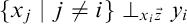 $\{ x_j \mid j\neq i \}\perp _{x_i\vec {z}}y_i$
by choosing the conjunct with
$\{ x_j \mid j\neq i \}\perp _{x_i\vec {z}}y_i$
by choosing the conjunct with
 $I = n\setminus \{i\}$
. Then we have
$I = n\setminus \{i\}$
. Then we have
 $$\begin{align*}\{ x_j \mid j\neq i \}\perp_{x_i\vec{z}}y_i \land y_i\perp_{\vec{x}\vec{z}}y_i. \end{align*}$$
Finally, the First Transitivity Rule yields
 $y_i\perp _{x_i\vec {z}}y_i$
, which means
$y_i\perp _{x_i\vec {z}}y_i$
, which means
 $\mathop {=}\hspace {-0.7pt}(x_i\vec {z}, y_i)$
.
$\mathop {=}\hspace {-0.7pt}(x_i\vec {z}, y_i)$
.
Lemma 3.16. Locality is equivalent to the formula
 $$\begin{align*}\left(\bigwedge_{I\subseteq n} \{ x_i \mid i\notin I \}\perp_{\{x_i \mid i\in I\}\vec{z}}\{y_i \mid i\in I\}\right) \land \left(\bigwedge_{i<n} y_i\perp_{\vec{x}\vec{z}}\{y_j \mid j\neq i\} \right). \end{align*}$$
In words, a hidden-variable team X supports locality if and only if it supports both parameter independence and outcome independence.
Proof It is essentially proved in [Reference Abramsky1] that the weaker version of parameter independence
 $$\begin{align*}\bigwedge_{i<n}\{x_j \mid j\neq i\}\perp_{x_i{\vec{z}}}y_i \end{align*}$$
together with outcome independence is equivalent to locality. What is left is to show that the stronger version of parameter independence still follows from locality. So suppose that X supports locality and fix
 $I\subseteq n$
. We show that
$I\subseteq n$
. We show that
 $$\begin{align*}X\models\{ x_i \mid i\notin I \}\perp_{\{x_i \mid i\in I\}\vec{z}}\{y_i \mid i\in I\}. \end{align*}$$
Let
 $s,s'\in X$
be such that
$s,s'\in X$
be such that
 $s(x_i\vec {z})=s'(x_i\vec {z})$
for all
$s(x_i\vec {z})=s'(x_i\vec {z})$
for all
 $i\in I$
. We wish to find
$i\in I$
. We wish to find
 $s"\in X$
with
$s"\in X$
with
 $s"({\vec {x}}{\vec {z}})=s({\vec {x}}{\vec {z}})$
and
$s"({\vec {x}}{\vec {z}})=s({\vec {x}}{\vec {z}})$
and
 $s"(\{y_i \mid i\in I\})=s'(\{y_i \mid i\in I\})$
. Let
$s"(\{y_i \mid i\in I\})=s'(\{y_i \mid i\in I\})$
. Let
 $s_i = s'$
for
$s_i = s'$
for
 $i\in I$
and
$i\in I$
and
 $s_i = s$
for
$s_i = s$
for
 $i\notin I$
. Now s is such that for
$i\notin I$
. Now s is such that for
 $i\in I$
,
$i\in I$
,
 $s(x_i\vec {z}) = s'(x_i\vec {z}) = s_i(x_i\vec {z})$
, but also for
$s(x_i\vec {z}) = s'(x_i\vec {z}) = s_i(x_i\vec {z})$
, but also for
 $i\notin I$
we have
$i\notin I$
we have
 $s(x_i\vec {z}) = s_i(x_i\vec {z})$
(as
$s(x_i\vec {z}) = s_i(x_i\vec {z})$
(as
 $s = s_i$
). Hence we have
$s = s_i$
). Hence we have
 $s(x_i\vec {z})=s_i(x_i\vec {z})$
for all
$s(x_i\vec {z})=s_i(x_i\vec {z})$
for all
 $i<n$
, so by locality there exists
$i<n$
, so by locality there exists
 $s"\in X$
with
$s"\in X$
with
 $s"(x_iy_i\vec {z}) = s_i(x_iy_i\vec {z})$
for all
$s"(x_iy_i\vec {z}) = s_i(x_iy_i\vec {z})$
for all
 $i<n$
. But then
$i<n$
. But then
 $s"(x_i{\vec {z}}) = s_i(x_i\vec {z}) = s(x_i\vec {z})$
for all
$s"(x_i{\vec {z}}) = s_i(x_i\vec {z}) = s(x_i\vec {z})$
for all
 $i<n$
and
$i<n$
and
 $s"(y_i) = s_i(y_i) = s'(y_i)$
for
$s"(y_i) = s_i(y_i) = s'(y_i)$
for
 $i\in I$
. Thus
$i\in I$
. Thus
 $s"$
is as desired.
$s"$
is as desired.
Next we indicate connections between properties of empirical teams and properties of hidden-variable teams, again following [Reference Abramsky1].
Proposition 3.17. The sentence
 $\tilde \exists z_0\exists z_1\dots \exists z_{l-1} \mathop {=}\hspace {-0.7pt}(\vec {z})$
is valid. More generally, if the variables
$\tilde \exists z_0\exists z_1\dots \exists z_{l-1} \mathop {=}\hspace {-0.7pt}(\vec {z})$
is valid. More generally, if the variables
 $\vec {z}$
do not occur in
$\vec {z}$
do not occur in
 $\varphi $
, then
$\varphi $
, then
 $\varphi \vdash \tilde \exists z_0\exists z_1\dots \exists z_{l-1} (\mathop {=}\hspace {-0.7pt}(\vec {z})\wedge \varphi )$
.
$\varphi \vdash \tilde \exists z_0\exists z_1\dots \exists z_{l-1} (\mathop {=}\hspace {-0.7pt}(\vec {z})\wedge \varphi )$
.
In words, every empirical team is realized by a hidden-variable team supporting single-valuedness.
Proof By the Reflexivity Rule, we have
 $\vec {z}\perp _{\vec {z}}\vec {z}$
. Using introduction of existential quantifier l times, we obtain
$\vec {z}\perp _{\vec {z}}\vec {z}$
. Using introduction of existential quantifier l times, we obtain
 $\exists z_0\dots \exists z_{l-1}\ \vec {z}\perp _{\vec {z}}\vec {z}$
. Using elimination of existential quantifier and introduction of dependence l times, we obtain
$\exists z_0\dots \exists z_{l-1}\ \vec {z}\perp _{\vec {z}}\vec {z}$
. Using elimination of existential quantifier and introduction of dependence l times, we obtain
 $$\begin{align*}\exists z_0\dots\exists z_{l-1}\left(\bigwedge_{k<l}\mathop{=}\hspace{-0.7pt}(z_k)\land\vec{z}\perp_{\vec{z}}\vec{z}\right). \end{align*}$$
As, from Armstrong’s axioms, one can infer
 $\bigwedge _{k<l}\mathop {=}\hspace {-0.7pt}(z_k)\vdash \mathop {=}\hspace {-0.7pt}(\vec {z})$
, we then easily obtain
$\bigwedge _{k<l}\mathop {=}\hspace {-0.7pt}(z_k)\vdash \mathop {=}\hspace {-0.7pt}(\vec {z})$
, we then easily obtain
 $\exists \vec {z}\mathop {=}\hspace {-0.7pt}(\vec {z})$
. Then, assuming
$\exists \vec {z}\mathop {=}\hspace {-0.7pt}(\vec {z})$
. Then, assuming
 $\varphi $
, by using elimination and introduction of existential quantifier l times, we obtain
$\varphi $
, by using elimination and introduction of existential quantifier l times, we obtain
 $\exists \vec {z}(\mathop {=}\hspace {-0.7pt}(\vec {z})\land \varphi )$
. Finally, the first introduction rule of
$\exists \vec {z}(\mathop {=}\hspace {-0.7pt}(\vec {z})\land \varphi )$
. Finally, the first introduction rule of
 $\tilde \exists $
gives
$\tilde \exists $
gives
 $\tilde \exists z_0\exists z_1\dots \exists z_{l-1} (\mathop {=}\hspace {-0.7pt}(\vec {z})\wedge \varphi )$
.
$\tilde \exists z_0\exists z_1\dots \exists z_{l-1} (\mathop {=}\hspace {-0.7pt}(\vec {z})\wedge \varphi )$
.
Proposition 3.18. Let
 $$\begin{align*}\varphi = \bigwedge_{I\subseteq n}\{x_i \mid i\notin I\}\perp_{\{x_i\mid i\in I\}}\{y_i \mid i\in I\} \end{align*}$$
and
 $$\begin{align*}\psi = \tilde{\exists}z_0\exists z_1\dots\exists z_{l-1} \left( \vec{z}\perp\vec{x} \land \bigwedge_{I\subseteq n} \{x_i \mid i\notin I\}\perp_{\{x_i\mid i\in I\}\vec{z}}\{y_i\mid i\in I\} \right). \end{align*}$$
Then
 $\varphi \dashv \vdash \psi $
.
$\varphi \dashv \vdash \psi $
.
In words, an empirical team supports no-signalling if and only if it can be realized by a hidden-variable team supporting
 ${\vec {z}}$
-independence and parameter independence.
${\vec {z}}$
-independence and parameter independence.
Proof We first show that
 $\varphi \vdash \psi $
. First of all, assume
$\varphi \vdash \psi $
. First of all, assume
 $\mathop {=}\hspace {-0.7pt}({\vec {z}})$
, which is harmless in view of Proposition 3.17. Note that
$\mathop {=}\hspace {-0.7pt}({\vec {z}})$
, which is harmless in view of Proposition 3.17. Note that
 $\mathop {=}\hspace {-0.7pt}({\vec {z}})$
means
$\mathop {=}\hspace {-0.7pt}({\vec {z}})$
means
 $\vec z\perp \vec z$
. By the Constancy Rule,
$\vec z\perp \vec z$
. By the Constancy Rule,
 $\vec z\perp \vec z$
entails
$\vec z\perp \vec z$
entails
 $\vec z\perp \vec x$
. Then fix
$\vec z\perp \vec x$
. Then fix
 $I\subseteq n$
. Note that
$I\subseteq n$
. Note that
 $\mathop {=}\hspace {-0.7pt}({\vec {z}})$
also means
$\mathop {=}\hspace {-0.7pt}({\vec {z}})$
also means
 $\mathop {=}\hspace {-0.7pt}(\emptyset ,{\vec {z}})$
. Now from Armstrong’s axioms, one can obtain
$\mathop {=}\hspace {-0.7pt}(\emptyset ,{\vec {z}})$
. Now from Armstrong’s axioms, one can obtain
 $\mathop {=}\hspace {-0.7pt}(\vec w,{\vec {z}})$
for any variable tuple
$\mathop {=}\hspace {-0.7pt}(\vec w,{\vec {z}})$
for any variable tuple
 $\vec w$
, in particular, when
$\vec w$
, in particular, when
 $\vec w = \{x_i \mid i\in I\}\cup \{y_i \mid i\in I\}$
. Now
$\vec w = \{x_i \mid i\in I\}\cup \{y_i \mid i\in I\}$
. Now
 $\mathop {=}\hspace {-0.7pt}(\{x_i \mid i\in I\}\{y_i \mid i\in I\},\vec z)$
means
$\mathop {=}\hspace {-0.7pt}(\{x_i \mid i\in I\}\{y_i \mid i\in I\},\vec z)$
means
 $\vec z\perp _{\{x_i \mid i\in I\}\{y_i \mid i\in I\}}\vec z$
. By the Constancy Rule,
$\vec z\perp _{\{x_i \mid i\in I\}\{y_i \mid i\in I\}}\vec z$
. By the Constancy Rule,
 $\vec z\perp _{\{x_i \mid i\in I\}\{y_i \mid i\in I\}}\vec z$
entails
$\vec z\perp _{\{x_i \mid i\in I\}\{y_i \mid i\in I\}}\vec z$
entails
 $\{x_i \mid i\notin I\}\perp _{\{x_i \mid i\in I\}\{y_i \mid i\in I\}}\vec z$
. Then by Contraction,
$\{x_i \mid i\notin I\}\perp _{\{x_i \mid i\in I\}\{y_i \mid i\in I\}}\vec z$
. Then by Contraction,
 $\{x_i \mid i\notin I\}\perp _{\{x_i \mid i\in I\}}\{y_i \mid i\in I\}$
and
$\{x_i \mid i\notin I\}\perp _{\{x_i \mid i\in I\}}\{y_i \mid i\in I\}$
and
 $\{x_i \mid i\notin I\}\perp _{\{x_i \mid i\in I\}\{y_i \mid i\in I\}}\vec z$
together entail
$\{x_i \mid i\notin I\}\perp _{\{x_i \mid i\in I\}\{y_i \mid i\in I\}}\vec z$
together entail
 $\{ x_i \mid i\notin I \}\perp _{\{x_i \mid i\in I\}}\{y_i \mid i\in I\}\vec {z}$
, which by Weak Union entails
$\{ x_i \mid i\notin I \}\perp _{\{x_i \mid i\in I\}}\{y_i \mid i\in I\}\vec {z}$
, which by Weak Union entails
 $\{ x_i \mid i\notin I \}\perp _{\{x_i \mid i\in I\}\vec {z}}\{y_i \mid i\in I\}$
.
$\{ x_i \mid i\notin I \}\perp _{\{x_i \mid i\in I\}\vec {z}}\{y_i \mid i\in I\}$
.
Hence from the assumptions
 $\mathop {=}\hspace {-0.7pt}(\vec z)$
and
$\mathop {=}\hspace {-0.7pt}(\vec z)$
and
 ${\{x_i \mid i\notin I\}\perp _{\{x_i \mid i\in I\}}\{y_i \mid i\in I\}}$
, we can deduce
${\{x_i \mid i\notin I\}\perp _{\{x_i \mid i\in I\}}\{y_i \mid i\in I\}}$
, we can deduce
 $\vec z\perp \vec x \land \{ x_i \mid i\notin I \}\perp _{\{x_i \mid i\in I\}\vec {z}}\{y_i \mid i\in I\}$
. Introducing conjunctions and existential quantifiers, we obtain that
$\vec z\perp \vec x \land \{ x_i \mid i\notin I \}\perp _{\{x_i \mid i\in I\}\vec {z}}\{y_i \mid i\in I\}$
. Introducing conjunctions and existential quantifiers, we obtain that
 $\mathop {=}\hspace {-0.7pt}({\vec {z}})$
and
$\mathop {=}\hspace {-0.7pt}({\vec {z}})$
and
 $\varphi $
entail
$\varphi $
entail
 $$\begin{align*}\exists z_0\dots\exists z_{l-1} \left( \vec{z}\perp\vec{x} \land \bigwedge_{I\subseteq n} \{x_i \mid i\notin I\}\perp_{\{x_i\mid i\in I\}\vec{z}}\{y_i\mid i\in I\} \right), \end{align*}$$
and hence by eliminating the existential quantifiers of the formula
 $\exists z_0\dots \exists z_{l-1}\mathop {=}\hspace {-0.7pt}(\vec z)$
, we obtain that
$\exists z_0\dots \exists z_{l-1}\mathop {=}\hspace {-0.7pt}(\vec z)$
, we obtain that
 $\exists z_0\dots \exists z_{l-1}\mathop {=}\hspace {-0.7pt}(\vec z)$
and
$\exists z_0\dots \exists z_{l-1}\mathop {=}\hspace {-0.7pt}(\vec z)$
and
 $\varphi $
together entail
$\varphi $
together entail
 $$\begin{align*}\exists z_0\dots\exists z_{l-1} \left( \vec{z}\perp\vec{x} \land \bigwedge_{I\subseteq n}\{x_i \mid i\notin I\}\perp_{\{x_i\mid i\in I\}{\vec{z}}}\{y_i \mid i\in I\} \right). \end{align*}$$
Then the elimination rule of
 $\tilde \exists $
gives that
$\tilde \exists $
gives that
 $\tilde \exists z_0\exists z_1\dots \exists z_{l-1}\mathop {=}\hspace {-0.7pt}(\vec z)$
and
$\tilde \exists z_0\exists z_1\dots \exists z_{l-1}\mathop {=}\hspace {-0.7pt}(\vec z)$
and
 $\varphi $
entail
$\varphi $
entail
 $\psi $
. As
$\psi $
. As
 $\tilde \exists z_0\exists z_1\dots \exists z_{l-1}\mathop {=}\hspace {-0.7pt}(\vec z)$
can be deduced with no assumptions, we obtain the desired deduction.
$\tilde \exists z_0\exists z_1\dots \exists z_{l-1}\mathop {=}\hspace {-0.7pt}(\vec z)$
can be deduced with no assumptions, we obtain the desired deduction.
Next we show that
 $\psi \vdash \varphi $
. Given
$\psi \vdash \varphi $
. Given
 $I\subseteq n$
, consider the assumptions
$I\subseteq n$
, consider the assumptions
 ${\vec {z}\perp \vec {x}}$
and
${\vec {z}\perp \vec {x}}$
and
 $\{ x_i \mid i\notin I \}\perp _{\{x_i\mid i\in I\}\vec {z}}\{y_i \mid i\in I\}$
. By Weak Union, Permutation, and Symmetry, from
$\{ x_i \mid i\notin I \}\perp _{\{x_i\mid i\in I\}\vec {z}}\{y_i \mid i\in I\}$
. By Weak Union, Permutation, and Symmetry, from
 $\vec z\perp \vec x$
, we obtain
$\vec z\perp \vec x$
, we obtain
 $\{ x_i \mid i\notin I \}\perp _{\{ x_i \mid i\in I \}}\vec z$
. From
$\{ x_i \mid i\notin I \}\perp _{\{ x_i \mid i\in I \}}\vec z$
. From
 $\{ x_i \mid i\notin I \}\perp _{\{ x_i \mid i\in I \}}\vec z$
and
$\{ x_i \mid i\notin I \}\perp _{\{ x_i \mid i\in I \}}\vec z$
and
 $\{x_i \mid i\notin I\}\perp _{\{x_i\mid i\in I\}\vec {z}}\{y_i\mid i\in I\}$
, Contraction gives
$\{x_i \mid i\notin I\}\perp _{\{x_i\mid i\in I\}\vec {z}}\{y_i\mid i\in I\}$
, Contraction gives
 $\{x_i \mid i\notin I\}\perp _{\{x_i\mid i\in I\}}\{y_i\mid i\in I\}{\vec {z}}$
, whence the Weakening Rule yields
$\{x_i \mid i\notin I\}\perp _{\{x_i\mid i\in I\}}\{y_i\mid i\in I\}{\vec {z}}$
, whence the Weakening Rule yields
 $\{x_i \mid i\notin I\}\perp _{\{x_i\mid i\in I\}}\{y_i\mid i\in I\}$
. Introducing conjunctions,
$\{x_i \mid i\notin I\}\perp _{\{x_i\mid i\in I\}}\{y_i\mid i\in I\}$
. Introducing conjunctions,
 $\vec {z}\perp \vec {x}$
together with
$\vec {z}\perp \vec {x}$
together with
 $\bigwedge _{I\subseteq n} \{x_i \mid i\notin I\}\perp _{\{x_i\mid i\in I\}\vec {z}}\{y_i\mid i\in I\}$
entails
$\bigwedge _{I\subseteq n} \{x_i \mid i\notin I\}\perp _{\{x_i\mid i\in I\}\vec {z}}\{y_i\mid i\in I\}$
entails
 $\bigwedge _{I\subseteq n} \{x_i \mid i\notin I\}\perp _{\{x_i\mid i\in I\}}\{y_i\mid i\in I\}$
, so by elimination of existential quantifiers in
$\bigwedge _{I\subseteq n} \{x_i \mid i\notin I\}\perp _{\{x_i\mid i\in I\}}\{y_i\mid i\in I\}$
, so by elimination of existential quantifiers in
 $\exists z_0\dots \exists z_{l-1} ( \vec {z}\perp \vec {x} \land \bigwedge _{I\subseteq n} \{x_i \mid i\notin I\}\perp _{\{x_i\mid i\in I\}\vec {z}}\{y_i\mid i\in I\} )$
, we obtain the deduction
$\exists z_0\dots \exists z_{l-1} ( \vec {z}\perp \vec {x} \land \bigwedge _{I\subseteq n} \{x_i \mid i\notin I\}\perp _{\{x_i\mid i\in I\}\vec {z}}\{y_i\mid i\in I\} )$
, we obtain the deduction
 $\exists z_0\dots \exists z_{l-1} ( \vec {z}\perp \vec {x} \land \bigwedge _{I\subseteq n} \{x_i \mid i\notin I\}\perp _{\{x_i\mid i\in I\}\vec {z}}\{y_i\mid i\in I\} )$
 $\vdash \varphi $
. By the elimination rule of
$\vdash \varphi $
. By the elimination rule of
 $\tilde \exists $
,
$\tilde \exists $
,
 $\psi \vdash \varphi $
finally follows.
$\psi \vdash \varphi $
finally follows.
Proposition 3.19. The formula
 $\tilde {\exists }z_0\exists z_1\dots \exists z_{l-1}\bigwedge _{i<n}\mathop {=}\hspace {-0.7pt}(x_i\vec {z},y_i)$
is valid. More generally,
$\tilde {\exists }z_0\exists z_1\dots \exists z_{l-1}\bigwedge _{i<n}\mathop {=}\hspace {-0.7pt}(x_i\vec {z},y_i)$
is valid. More generally,
 $\varphi \models \tilde {\exists }z_0\exists z_1\dots \exists z_{l-1}(\bigwedge _{i<n}\mathop {=}\hspace {-0.7pt}(x_i\vec {z},y_i)\wedge \varphi )$
, when
$\varphi \models \tilde {\exists }z_0\exists z_1\dots \exists z_{l-1}(\bigwedge _{i<n}\mathop {=}\hspace {-0.7pt}(x_i\vec {z},y_i)\wedge \varphi )$
, when
 $\vec {z}$
does not occur free in
$\vec {z}$
does not occur free in
 $\varphi $
.
$\varphi $
.
In words, every empirical team is realized by a hidden-variable team supporting strong determinism.
Proof Essentially proved in [Reference Abramsky1].
Remark 3.20. Note that while the formula
 $\tilde {\exists }z_0\exists z_1\dots \exists z_{l-1}\bigwedge _{i<n}\mathop {=}\hspace {-0.7pt}(x_i\vec {z},y_i)$
is valid, the formula
$\tilde {\exists }z_0\exists z_1\dots \exists z_{l-1}\bigwedge _{i<n}\mathop {=}\hspace {-0.7pt}(x_i\vec {z},y_i)$
is valid, the formula
 $\exists z_0\dots \exists z_{l-1}\bigwedge _{i<n}\mathop {=}\hspace {-0.7pt}(x_i\vec {z},y_i)$
may not be, as demonstrated by the simple counter-example in the case where
$\exists z_0\dots \exists z_{l-1}\bigwedge _{i<n}\mathop {=}\hspace {-0.7pt}(x_i\vec {z},y_i)$
may not be, as demonstrated by the simple counter-example in the case where
 $n = 4$
and
$n = 4$
and
 $l=1$
: the domain of the structure is
$l=1$
: the domain of the structure is
 $\{0,1\}$
, and the team is the full team
$\{0,1\}$
, and the team is the full team
 $\{0,1\}^{V_{\text {m}}\cup V_{\text {o}}}$
. It would seem that this problem could be overcome by increasing the length of the hidden-variable tuple: a sufficient condition for
$\{0,1\}^{V_{\text {m}}\cup V_{\text {o}}}$
. It would seem that this problem could be overcome by increasing the length of the hidden-variable tuple: a sufficient condition for
 $\exists z_0\dots \exists z_{l-1}\bigwedge _{i<n}\mathop {=}\hspace {-0.7pt}(x_i\vec {z},y_i)$
to be satisfied is that
$\exists z_0\dots \exists z_{l-1}\bigwedge _{i<n}\mathop {=}\hspace {-0.7pt}(x_i\vec {z},y_i)$
to be satisfied is that
 $\vec z$
can be assigned enough values to make each value of
$\vec z$
can be assigned enough values to make each value of
 $x_i\vec z$
unique for all
$x_i\vec z$
unique for all
 $i<n$
, whence
$i<n$
, whence
 $\mathop {=}\hspace {-0.7pt}(x_i\vec {z},y_i)$
is trivially satisfied.
$\mathop {=}\hspace {-0.7pt}(x_i\vec {z},y_i)$
is trivially satisfied.
Proposition 3.21. The formula
 $\tilde {\exists }z_0\exists z_1\dots \exists z_{l-1}(\mathop {=}\hspace {-0.7pt}(\vec {x}\vec {z},\vec {y})\land \vec {z}\perp \vec {x})$
is valid. More generally,
$\tilde {\exists }z_0\exists z_1\dots \exists z_{l-1}(\mathop {=}\hspace {-0.7pt}(\vec {x}\vec {z},\vec {y})\land \vec {z}\perp \vec {x})$
is valid. More generally,
 $\varphi \models \tilde {\exists }z_0\exists z_1\dots \exists z_{l-1}(\mathop {=}\hspace {-0.7pt}(\vec {x}\vec {z},\vec {y})\land \vec {z}\perp \vec {x}\wedge \varphi )$
, when
$\varphi \models \tilde {\exists }z_0\exists z_1\dots \exists z_{l-1}(\mathop {=}\hspace {-0.7pt}(\vec {x}\vec {z},\vec {y})\land \vec {z}\perp \vec {x}\wedge \varphi )$
, when
 $\vec {z}$
does not occur free in
$\vec {z}$
does not occur free in
 $\varphi $
.
$\varphi $
.
In words, every empirical team is realized by a hidden-variable team supporting weak determinism and
 ${\vec {z}}$
-independence.
${\vec {z}}$
-independence.
Proof Essentially proved in [Reference Abramsky1].
Proposition 3.22. Let
 $$ \begin{align*} \varphi &= \bigwedge_{I\subseteq n}\left( \{x_i \mid i\notin I\}\perp_{\{x_i\mid i\in I\}\vec{z}}\{y_i\mid i\in I\} \right), \\ \psi &= \bigwedge_{i<n}\left( y_i\perp_{\vec{x}\vec{z}}\{y_j \mid j\neq i \} \right) \text{ and} \\ \theta &= \bigwedge_{i<n} \mathop{=}\hspace{-0.7pt}(x_i\vec{z},y_i). \end{align*} $$
Then
 $\tilde {\exists }z_0\exists z_1\dots \exists z_{l-1}({\vec {z}}\perp {\vec {x}}\land \varphi \land \psi ) \models \tilde {\exists }z_0\exists z_1\dots \exists z_{l-1}({\vec {z}}\perp {\vec {x}}\land \theta )$
.
$\tilde {\exists }z_0\exists z_1\dots \exists z_{l-1}({\vec {z}}\perp {\vec {x}}\land \varphi \land \psi ) \models \tilde {\exists }z_0\exists z_1\dots \exists z_{l-1}({\vec {z}}\perp {\vec {x}}\land \theta )$
.
In words, any hidden-variable team supporting
 ${\vec {z}}$
-independence and locality is equivalent (in the sense of Definition 3.2) to a hidden-variable team supporting
${\vec {z}}$
-independence and locality is equivalent (in the sense of Definition 3.2) to a hidden-variable team supporting
 ${\vec {z}}$
-independence and strong determinism.
${\vec {z}}$
-independence and strong determinism.
Proof Essentially proved in [Reference Abramsky1].
We do not know whether the logical consequences of Propositions 3.19–3.22 are provable from our axioms. This is a subject of further study. Remark 3.20 would suggest that stronger axioms for
 $\tilde \exists $
be required, as the semantic proofs of these propositions make use of the possibility of acquiring values for the hidden variables
$\tilde \exists $
be required, as the semantic proofs of these propositions make use of the possibility of acquiring values for the hidden variables
 ${\vec {z}}$
outside of the values that are possible for
${\vec {z}}$
outside of the values that are possible for
 ${\vec {x}}$
and
${\vec {x}}$
and
 ${\vec {y}}$
.
${\vec {y}}$
.
3.5 Representation of no-go theorems in team semantics
We now turn to the representation of no-go theorems in the foundations of quantum mechanics in terms of team semantics. These results have fundamental significance, both foundationally, and also for their implications for quantum information and computation. They rule out the possibility, even in principle, of accounting for quantum behaviour by means of local hidden-variable theories. This shows that the behaviour of quantum mechanics is essentially and unavoidably non-local. This non-locality is, on the one hand, highly challenging in terms of understanding what quantum mechanics is telling us about the nature of physical reality. On the other hand, this non-classicality opens up the possibility of performing information processing tasks using quantum resources which provably exceed what can be done classically.
How can these no-go theorems be represented in terms of team semantics? All the results so far are examples of logical consequences and equivalences between team properties (or formulas). To prove the no-go theorems, we shall exhibit some counter-example teams that demonstrate certain failures of logical consequence. These failures will imply the impossibility of describing these teams in terms of local hidden variables. As we shall see later, these teams do arise as behaviours of certain quantum mechanical systems.
The original result in this line is the celebrated Bell’s Theorem [Reference Bell9]. However, that result in its original form is probabilistic in character, and hence not amenable to formalization in terms of team semantics.Footnote 6 Two later constructions, due to Greenberger–Horne–Zeilinger (GHZ) [Reference Greenberger, Horne, Shimony and Zeilinger22, Reference Liu, Zhou, Meng, Yang, Li, Meng, Su, Chen, Sun, Xu, Li and Guo37] and Hardy [Reference Hardy27], strengthen Bell’s result by constructions which work at the purely possibilistic level, and hence can be formalized directly in team semantics.
In Tarski semantics of first-order logic, some existential formulas, such as
 $\exists z (x=z \land \neg y=z)$
, are not valid while others, such as
$\exists z (x=z \land \neg y=z)$
, are not valid while others, such as
 $\exists z (x=z \lor x=y)$
, are. To decide which are valid and which are not is particularly simple, especially in the empty vocabulary because first-order logic has in that case elimination of quantifiers. In team semantics where such quantifier elimination is not known to be possible, non-valid existential-conjunctive formulas can be quite complicated, as the examples below show. As we shall see, the no-go results of quantum mechanics give rise to very interesting teams.
$\exists z (x=z \lor x=y)$
, are. To decide which are valid and which are not is particularly simple, especially in the empty vocabulary because first-order logic has in that case elimination of quantifiers. In team semantics where such quantifier elimination is not known to be possible, non-valid existential-conjunctive formulas can be quite complicated, as the examples below show. As we shall see, the no-go results of quantum mechanics give rise to very interesting teams.
We turn firstly to the GHZ construction.
Definition 3.23. Assume that
 $n=3$
. Let X be an empirical team with
$n=3$
. Let X be an empirical team with
 $\operatorname {\mathrm {rng}}(X) = \{0,1\}$
. Denote
$\operatorname {\mathrm {rng}}(X) = \{0,1\}$
. Denote
 $$ \begin{align*} P &= \{(0,1,1), (1,0,1), (1,1,0)\}, \\ Q &= \{(0,0,0), (0,1,1), (1,0,1), (1,1,0)\} \text{ and}\\ R &= \{(0,0,1), (0,1,0), (1,0,0), (1,1,1)\}. \end{align*} $$
We say that X is a GHZ team if it satisfies the following conditions.
-
(i)
$Q = \{s(\vec {y}) \mid s\in X, s(\vec {x})\in P\}$
and
$P \subseteq \{s(\vec {x}) \mid s\in X, s(\vec {y})\in Q\}$
. -
(ii)
$R = \{s(\vec {y}) \mid s\in X, s(\vec {x}) = (0,0,0)\}$
.


The following is a minimal example of a GHZ team:

The following is like [Reference Abramsky1, Proposition 6.2].
Proposition 3.24. The formula
 $\tilde {\exists }z_0\exists z_1\dots \exists z_{l-1}({\vec {z}}\perp {\vec {x}}\land \varphi \land \psi )$
, where
$\tilde {\exists }z_0\exists z_1\dots \exists z_{l-1}({\vec {z}}\perp {\vec {x}}\land \varphi \land \psi )$
, where
 $$ \begin{align*} \varphi &= \bigwedge_{I\subseteq n}\left( \{x_i \mid i\notin I\}\perp_{\{x_i\mid i\in I\}\vec{z}}\{y_i\mid i\in I\} \right) \text{ and} \\ \psi &= \bigwedge_{i<n}\left( y_i\perp_{\vec{x}\vec{z}}\{y_j \mid j\neq i \} \right), \end{align*} $$
is not valid, as demonstrated by any GHZ team.
In words, no GHZ team can be realized by a hidden-variable team supporting
 ${\vec {z}}$
-independence and locality.
${\vec {z}}$
-independence and locality.
Proof Proved in [Reference Abramsky1].
Next, we consider the Hardy construction.
Definition 3.25. Assume that
 $n=2$
. Let X be an empirical team with
$n=2$
. Let X be an empirical team with
 $\operatorname {\mathrm {rng}}(X) = \{0,1\}$
. Let
$\operatorname {\mathrm {rng}}(X) = \{0,1\}$
. Let
 $s_0,\dots ,s_3$
be as in the following table.
$s_0,\dots ,s_3$
be as in the following table.

We say that X is a Hardy team if the following hold:
-
(i)
$s_0\in X$
but
$s_1,s_2,s_3\notin X$
, and -
(ii) for every pair
$\vec {a}\in \{0,1\}^2$
, there is some
$s\in X$
with
$s(\vec {x})=\vec {a}$
.Footnote
7


A minimal example of a Hardy team would be the following:

The following is like [Reference Abramsky1, Proposition 6.3].
Proposition 3.26. No Hardy team can be realized by a hidden-variable team supporting
 ${\vec {z}}$
-independence and locality.
${\vec {z}}$
-independence and locality.
Theorem 3.26 gives an alternative proof that the formula in Theorem 3.24 is not valid.
Proof of Proposition 3.26
Proved in [Reference Abramsky1].
3.5.1. Discussion
We emphasize that the choice of specific counter-example teams for these results is significant, since to apply the results to quantum mechanics, we must show that these specific teams can be realized in quantum mechanics. We shall discuss quantum-realizability in Section 5.
Our reason for discussing both the GHZ and Hardy constructions is that they exhibit different “strengths” of non-locality. The GHZ construction exhibits a maximal form of non-locality; note that it requires at least a tripartite system (the construction can be generalized straightforwardly to n-partite systems for
 $n> 3$
). The Hardy construction only requires a bipartite system, but exhibits a weaker form of non-locality. Both are stronger than the original probabilistic form of Bell’s theorem in [Reference Bell9]. For a detailed discussion of this hierarchy, see [Reference Abramsky and Brandenburger3].
$n> 3$
). The Hardy construction only requires a bipartite system, but exhibits a weaker form of non-locality. Both are stronger than the original probabilistic form of Bell’s theorem in [Reference Bell9]. For a detailed discussion of this hierarchy, see [Reference Abramsky and Brandenburger3].
The Kochen–Specker construction [Reference Kochen and Specker34] gives an example of an empirical model which cannot be realized by any hidden-variable model supporting
 ${\vec {z}}$
-independence and parameter independence, providing a result even stronger than Propositions 3.24 and 3.26. However, the model in question does not quite fit our framework, which deals with so-called Bell-type scenarios. A sheaf-theoretic framework is given in [Reference Abramsky and Brandenburger3], which subsumes both non-locality arguments for Bell scenarios, and contextuality proofs exemplified by the Kochen–Specker construction. This could be translated into the language of team semantics using some version of the polyteam semantics of [Reference Hannula, Kontinen and Virtema26]. A polyteam is essentially a set of teams. A simple example is the combination of a team describing lecture courses in an academic department, with variables for course name and course lecturer, and a different personnel team with variables for lectures and their office hours. Polyteams seem to be a suitable framework which allows a team semantics analysis of the sheaf-theoretic framework of [Reference Abramsky and Brandenburger3], and hence enables a treatment of the Kochen–Specker Theorem and related results. We shall leave the elaboration of this idea to future work.
${\vec {z}}$
-independence and parameter independence, providing a result even stronger than Propositions 3.24 and 3.26. However, the model in question does not quite fit our framework, which deals with so-called Bell-type scenarios. A sheaf-theoretic framework is given in [Reference Abramsky and Brandenburger3], which subsumes both non-locality arguments for Bell scenarios, and contextuality proofs exemplified by the Kochen–Specker construction. This could be translated into the language of team semantics using some version of the polyteam semantics of [Reference Hannula, Kontinen and Virtema26]. A polyteam is essentially a set of teams. A simple example is the combination of a team describing lecture courses in an academic department, with variables for course name and course lecturer, and a different personnel team with variables for lectures and their office hours. Polyteams seem to be a suitable framework which allows a team semantics analysis of the sheaf-theoretic framework of [Reference Abramsky and Brandenburger3], and hence enables a treatment of the Kochen–Specker Theorem and related results. We shall leave the elaboration of this idea to future work.
4 Independence logic in probabilistic and K-team semantics
We show that the probabilistic framework of Brandenburger and Yanofsky [Reference Brandenburger and Yanofsky10] can be translated to the language of probabilistic team semantics exactly the same way that the purely relational framework of [Reference Abramsky1] translates to ordinary team semantics. All the formal proofs of the relational setting turn out to be sound also in the probabilistic framework, as we are able to prove the validity of our axioms also in this setting, and even in K-team semantics for K a positive, commutative, and multiplicatively cancellative semiring. A semiring is multiplicatively cancellative if
 $ab = ac$
implies
$ab = ac$
implies
 $b = c$
whenever
$b = c$
whenever
 $a \neq 0$
. A result of Hannula [Reference Hannula24] shows that the so-called semigraphoid axioms are sound for such K, and Proposition 2.8 shows that our axioms are all provable from them.
$a \neq 0$
. A result of Hannula [Reference Hannula24] shows that the so-called semigraphoid axioms are sound for such K, and Proposition 2.8 shows that our axioms are all provable from them.
4.1 Probabilistic teams
So far, we have only been looking at possibilistic (i.e., two-valued relational) versions of the independence notions of quantum physics while these notions are usually taken to be probabilistic. To be able to discuss the probabilistic notions from the point of view of team semantics, we need a suitable framework. For this, we consider probabilistic team semantics.
The study of a probabilistic variant of independence logic was first done in a multiteam setting in [Reference Durand, Hannula, Kontinen, Meier and Virtema14]. Prior to that, multiteams were studied in [Reference Hyttinen, Paolini and Väänänen30, Reference Hyttinen, Paolini and Väänänen31, Reference Väänänen47]. Probabilistic teams were then introduced by Durand et al. in [Reference Durand, Hannula, Kontinen, Meier, Virtema, Ferrarotti and Woltran15] as a way to generalize multiteams, and further investigated in [Reference Hannula, Hirvonen, Kontinen, Kulikov and Virtema25]. They can be thought of as a special case of measure teams, another approach to probabilities in team semantics given in [Reference Hyttinen, Paolini and Väänänen31].
It should be observed that we are not introducing probabilistic logic in the sense of formulas having probabilities. In our approach, only the teams are probabilistic and the logic is two-valued.
Definition 4.1. Let A be a finite set and V a finite set of variables. A probabilistic team, with variable domain V and value domain A, is a probability distribution
 $\mathbb {X}\colon A^V \to [0,1]$
.
$\mathbb {X}\colon A^V \to [0,1]$
.
Let
 $\mathfrak {A}$
be a (possibly many-sorted) finite structure, and let X be the full team of
$\mathfrak {A}$
be a (possibly many-sorted) finite structure, and let X be the full team of
 $\mathfrak {A}$
with domain V. Then a probabilistic team of
$\mathfrak {A}$
with domain V. Then a probabilistic team of
 $\mathfrak {A}$
with variable domain V is any distribution
$\mathfrak {A}$
with variable domain V is any distribution
 $\mathbb {X}\colon X\to [0,1]$
.
$\mathbb {X}\colon X\to [0,1]$
.
Ordinary teams of size k can be seen as probabilistic teams by giving each assignment in the team probability
 $1/k$
and assignments not in the team probability zero. This idea of treating ordinary teams as uniformly distributed probabilistic teams generalizes to multiteams, i.e., teams in which assignments can have several occurrences. Then an assignment which occurs m times is given the probability
$1/k$
and assignments not in the team probability zero. This idea of treating ordinary teams as uniformly distributed probabilistic teams generalizes to multiteams, i.e., teams in which assignments can have several occurrences. Then an assignment which occurs m times is given the probability
 $m/k$
. In fact, it is not difficult to see that any probabilistic team with rational probabilities corresponds to a multiteam.
$m/k$
. In fact, it is not difficult to see that any probabilistic team with rational probabilities corresponds to a multiteam.
We will call a probabilistic team with variable domain
 $V_{\text {m}}\cup V_{\text {o}}$
a probabilistic empirical team and a probabilistic team with variable domain
$V_{\text {m}}\cup V_{\text {o}}$
a probabilistic empirical team and a probabilistic team with variable domain
 $V_{\text {m}}\cup V_{\text {o}}\cup V_{\text {h}}$
a probabilistic hidden-variable team.
$V_{\text {m}}\cup V_{\text {o}}\cup V_{\text {h}}$
a probabilistic hidden-variable team.
Definition 4.2. We say that a team X is the possibilistic collapse of a probabilistic team
 $\mathbb {X}$
if for any assignment s,
$\mathbb {X}$
if for any assignment s,
 $s\in X$
if and only if
$s\in X$
if and only if
 $\mathbb {X}(s)>0$
.
$\mathbb {X}(s)>0$
.
Note that if
 $\mathbb {X}$
is a probabilistic team of
$\mathbb {X}$
is a probabilistic team of
 $\mathfrak {A}$
, then the possibilistic collapse X is a team of
$\mathfrak {A}$
, then the possibilistic collapse X is a team of
 $\mathfrak {A}$
.
$\mathfrak {A}$
.
We may consider a probabilistic team a “probabilistic realization” of its collapse. Of course, an ordinary team has a multitude of such probabilistic realizations.
The possibilistic collapse of a probabilistic team
 $\mathbb {X}$
is also called the support of
$\mathbb {X}$
is also called the support of
 $\mathbb {X}$
and denoted by
$\mathbb {X}$
and denoted by
 $\operatorname {\mathrm {supp}}\mathbb {X}$
.
$\operatorname {\mathrm {supp}}\mathbb {X}$
.
We denote by
 $\left | \mathbb {X}_{\vec {u}=\vec {a}} \right |$
the number
$\left | \mathbb {X}_{\vec {u}=\vec {a}} \right |$
the number
 $$\begin{align*}\sum_{\substack{s(\vec{u})=\vec{a} \\ s\in\operatorname{\mathrm{supp}}\mathbb{X}}}\mathbb{X}(s), \end{align*}$$
i.e., the marginal probability of the variable tuple
 $\vec {u}$
having the value
$\vec {u}$
having the value
 $\vec {a}$
in
$\vec {a}$
in
 $\mathbb {X}$
.
$\mathbb {X}$
.
Next we define the probabilistic analogue for an empirical team being realized by a hidden-variable team.
Definition 4.3. A probabilistic hidden-variable team
 $\mathbb {Y}$
realizes a probabilistic empirical team
$\mathbb {Y}$
realizes a probabilistic empirical team
 $\mathbb {X}$
if for all
$\mathbb {X}$
if for all
 $\vec {a}$
and
$\vec {a}$
and
 $\vec {b}$
we have
$\vec {b}$
we have
-
(i)
$\left | \mathbb {X}_{\vec {x}=\vec {a}} \right | = 0$
if and only if
$\left | \mathbb {Y}_{\vec {x}=\vec {a}} \right | = 0$
, and -
(ii)
$\left | \mathbb {X}_{\vec {x}\vec {y}=\vec {a}\vec {b}} \right |\cdot \left | \mathbb {Y}_{\vec {x}=\vec {a}} \right | = \left | \mathbb {Y}_{\vec {x}\vec {y}=\vec {a}\vec {b}} \right |\cdot \left | \mathbb {X}_{\vec {x}=\vec {a}} \right |$
.
 $\mathbb {Y}$
uniformly realizes
$\mathbb {Y}$
uniformly realizes
 $\mathbb {X}$
if in addition
$\mathbb {X}$
if in addition
 $\left | \mathbb {X}_{\vec {x}=\vec {a}} \right |=\left | \mathbb {Y}_{\vec {x}=\vec {a}} \right |$
for all
$\left | \mathbb {X}_{\vec {x}=\vec {a}} \right |=\left | \mathbb {Y}_{\vec {x}=\vec {a}} \right |$
for all
 $\vec {a}$
.
$\vec {a}$
.
The intuition behind the definition is the following:
 $\mathbb {Y}$
realizes
$\mathbb {Y}$
realizes
 $\mathbb {X}$
if the probability of the event “
$\mathbb {X}$
if the probability of the event “
 $s(\vec {x})=\vec {a}\,$
” is non-zero in both teams exactly the same time, and in the case that the probability indeed is non-zero, the probability of the event “
$s(\vec {x})=\vec {a}\,$
” is non-zero in both teams exactly the same time, and in the case that the probability indeed is non-zero, the probability of the event “
 $s(\vec {y})=\vec {b}\,$
”, conditional to “
$s(\vec {y})=\vec {b}\,$
”, conditional to “
 $s(\vec {x})=\vec {a}\,$
”, is the same in both teams. Uniform realizability appears to be a stronger concept than realizability, but we do not have an example for that yet.
$s(\vec {x})=\vec {a}\,$
”, is the same in both teams. Uniform realizability appears to be a stronger concept than realizability, but we do not have an example for that yet.
Proposition 4.4. If
 $\kern1.5pt\mathbb {Y}$
realizes
$\kern1.5pt\mathbb {Y}$
realizes
 $\mathbb {X}$
, then the possibilistic collapse of
$\mathbb {X}$
, then the possibilistic collapse of
 $\kern1.7pt\mathbb {Y}$
realizes the possibilistic collapse of
$\kern1.7pt\mathbb {Y}$
realizes the possibilistic collapse of
 $\mathbb {X}$
.
$\mathbb {X}$
.
Proposition 4.4 says that one obtains the same team by first projecting away hidden variables and then taking the possibilistic collapse as one gets by first taking the possibilistic collapse and then projecting away the hidden variables, i.e., the diagram in Figure 1 commutes.
Probabilistic realization implies possibilistic realization.

Proof of Proposition 4.4
Suppose that
 $\mathbb {Y}$
realizes
$\mathbb {Y}$
realizes
 $\mathbb {X}$
, and denote by Y and X the respective possibilistic collapse. In order to prove that Y realizes X, we need to show that for all assignments s,
$\mathbb {X}$
, and denote by Y and X the respective possibilistic collapse. In order to prove that Y realizes X, we need to show that for all assignments s,
 $$\begin{align*}s\in X \iff \exists s'\in Y \bigwedge_{i<n}(s'(x_i)=s(x_i) \land s'(y_i)=s(y_i)). \end{align*}$$
We show only one direction, the other one is similar.
Suppose that
 $s\in X$
. Denote
$s\in X$
. Denote
 $\vec {a}=s(\vec {x})$
and
$\vec {a}=s(\vec {x})$
and
 $\vec {b}=s(\vec {y})$
. The aim is to show that there is some
$\vec {b}=s(\vec {y})$
. The aim is to show that there is some
 $s'\in Y$
with
$s'\in Y$
with
 $s'(\vec {x})=\vec {a}$
and
$s'(\vec {x})=\vec {a}$
and
 $s'(\vec {y})=\vec {b}$
. Since X is the possibilistic collapse of
$s'(\vec {y})=\vec {b}$
. Since X is the possibilistic collapse of
 $\mathbb {X}$
and
$\mathbb {X}$
and
 $s\in X$
, we have
$s\in X$
, we have
 $\mathbb {X}(s)>0$
, and as in addition
$\mathbb {X}(s)>0$
, and as in addition
 $s(\vec {x})=\vec {a}$
, we obtain
$s(\vec {x})=\vec {a}$
, we obtain
 $\left | \mathbb {X}_{\vec {x}=\vec {a}} \right |> 0$
. Thus, as
$\left | \mathbb {X}_{\vec {x}=\vec {a}} \right |> 0$
. Thus, as
 $\mathbb {Y}$
realizes
$\mathbb {Y}$
realizes
 $\mathbb {X}$
,
$\mathbb {X}$
,
 $\left | \mathbb {Y}_{\vec {x}=\vec {a}} \right |> 0$
. Similarly,
$\left | \mathbb {Y}_{\vec {x}=\vec {a}} \right |> 0$
. Similarly,
 $\left | \mathbb {X}_{\vec {x}\vec {y}=\vec {a}\vec {b}} \right |> 0$
, and as
$\left | \mathbb {X}_{\vec {x}\vec {y}=\vec {a}\vec {b}} \right |> 0$
, and as
 $$\begin{align*}\left| \mathbb{Y}_{\vec{x}\vec{y}=\vec{a}\vec{b}} \right| = \frac{\left| \mathbb{X}_{\vec{x}\vec{y}=\vec{a}\vec{b}} \right|\cdot\left| \mathbb{Y}_{\vec{x}=\vec{a}} \right|}{\left| \mathbb{X}_{\vec{x}=\vec{a}} \right|}, \end{align*}$$
also
 $\left | \mathbb {Y}_{\vec {x}\vec {y}=\vec {a}\vec {b}} \right |> 0$
. This means that there is some
$\left | \mathbb {Y}_{\vec {x}\vec {y}=\vec {a}\vec {b}} \right |> 0$
. This means that there is some
 $s'$
with
$s'$
with
 $\mathbb {Y}(s')> 0$
and
$\mathbb {Y}(s')> 0$
and
 $s'(\vec {x}\vec {y})=\vec {a}\vec {b}$
. Since Y is the possibilistic collapse of
$s'(\vec {x}\vec {y})=\vec {a}\vec {b}$
. Since Y is the possibilistic collapse of
 $\mathbb {Y}$
, this means that
$\mathbb {Y}$
, this means that
 $s'\in Y$
, as desired.
$s'\in Y$
, as desired.
4.2 Probabilistic independence logic
We now present the semantics of the probabilistic (conditional) independence atom
 $\vec {u}\mathbin {\perp \!\!\!\perp }_{\vec {v}}\vec {w}$
, as defined in [Reference Durand, Hannula, Kontinen, Meier, Virtema, Ferrarotti and Woltran15].
$\vec {u}\mathbin {\perp \!\!\!\perp }_{\vec {v}}\vec {w}$
, as defined in [Reference Durand, Hannula, Kontinen, Meier, Virtema, Ferrarotti and Woltran15].
Definition 4.5. Let
 $\mathfrak {A}$
be a structure and
$\mathfrak {A}$
be a structure and
 $\mathbb {X}$
a probabilistic team of
$\mathbb {X}$
a probabilistic team of
 $\mathfrak {A}$
, and let
$\mathfrak {A}$
, and let
 $\vec {u}$
,
$\vec {u}$
,
 $\vec {v}$
, and
$\vec {v}$
, and
 $\vec {w}$
be tuples of variables. Then
$\vec {w}$
be tuples of variables. Then
 $\mathbb {X}$
satisfies the formula
$\mathbb {X}$
satisfies the formula
 $\vec {u}\mathbin {\perp \!\!\!\perp }_{\vec {v}}\vec {w}$
in
$\vec {u}\mathbin {\perp \!\!\!\perp }_{\vec {v}}\vec {w}$
in
 $\mathfrak {A}$
, in symbols
$\mathfrak {A}$
, in symbols
 $\mathfrak {A}\models _{\mathbb {X}}\vec {u}\mathbin {\perp \!\!\!\perp }_{\vec {v}}\vec {w}$
, if for all
$\mathfrak {A}\models _{\mathbb {X}}\vec {u}\mathbin {\perp \!\!\!\perp }_{\vec {v}}\vec {w}$
, if for all
 $\vec {a}$
,
$\vec {a}$
,
 $\vec {b}$
, and
$\vec {b}$
, and
 $\vec {c}$
,
$\vec {c}$
,
 $$\begin{align*}\left| \mathbb{X}_{\vec{u}\vec{v}=\vec{a}\vec{b}} \right| \cdot \left| \mathbb{X}_{\vec{v}\vec{w}=\vec{b}\vec{c}} \right| = \left| \mathbb{X}_{\vec{u}\vec{v}\vec{w}=\vec{a}\vec{b}\vec{c}} \right| \cdot \left| \mathbb{X}_{\vec{v}=\vec{b}} \right|. \end{align*}$$
The intention behind the atom is to capture the notion of conditional independence in probability theory: denoting a probability measure by p, two events A and B are conditionally independent over an event C (assuming
 $p(C)>0$
) if
$p(C)>0$
) if
 $$\begin{align*}p(A\mid C)p(B\mid C) = p(A\cap B\mid C). \end{align*}$$
Recalling that
 $p(D\mid C) = p(D\cap C)/p(C)$
, we can multiply both sides of the equation by
$p(D\mid C) = p(D\cap C)/p(C)$
, we can multiply both sides of the equation by
 $p(C)^2$
and obtain
$p(C)^2$
and obtain
 $$\begin{align*}p(A\cap C)p(B\cap C) = p(A\cap B\cap C)p(C), \end{align*}$$
which is exactly what the probabilistic dependence atom expresses. In the case when
 $p(C)=0$
, both sides of the new equation are
$p(C)=0$
, both sides of the new equation are
 $0$
, so in that case, the independence atom is vacuously true.
$0$
, so in that case, the independence atom is vacuously true.
Exactly the same way as in ordinary independence logic, we can define the probabilistic dependence atom
 $\mathop {=}\hspace {-0.7pt}(\vec {v},\vec {w})$
via the independence atom.
$\mathop {=}\hspace {-0.7pt}(\vec {v},\vec {w})$
via the independence atom.
Definition 4.6. Let
 $\vec {v}$
and
$\vec {v}$
and
 $\vec {w}$
tuples of variables. Then by
$\vec {w}$
tuples of variables. Then by
 $\mathop {=}\hspace {-0.7pt}(\vec {v},\vec {w})$
we mean the formula
$\mathop {=}\hspace {-0.7pt}(\vec {v},\vec {w})$
we mean the formula
 $\vec {w}\mathbin {\perp \!\!\!\perp }_{\vec {v}}\vec {w}$
. By
$\vec {w}\mathbin {\perp \!\!\!\perp }_{\vec {v}}\vec {w}$
. By
 $\mathop {=}\hspace {-0.7pt}(\vec {w}),$
we mean the formula
$\mathop {=}\hspace {-0.7pt}(\vec {w}),$
we mean the formula
 $\vec {w}\mathbin {\perp \!\!\!\perp }\vec {w}$
and call it the probabilistic constancy atom.
$\vec {w}\mathbin {\perp \!\!\!\perp }\vec {w}$
and call it the probabilistic constancy atom.
The syntax of probabilistic independence logic is the same as the syntax of ordinary independence logic, except that we use the symbol
 $\mathbin {\perp \!\!\!\perp }$
instead of
$\mathbin {\perp \!\!\!\perp }$
instead of
 $\perp $
. Next we present the semantics of more complex formulas of probabilistic independence logic, as defined in [Reference Durand, Hannula, Kontinen, Meier, Virtema, Ferrarotti and Woltran15]. First we define the r-scaled union
$\perp $
. Next we present the semantics of more complex formulas of probabilistic independence logic, as defined in [Reference Durand, Hannula, Kontinen, Meier, Virtema, Ferrarotti and Woltran15]. First we define the r-scaled union
 $\mathbb {X}\sqcup _r\mathbb {Y}$
of two probabilistic teams
$\mathbb {X}\sqcup _r\mathbb {Y}$
of two probabilistic teams
 $\mathbb {X}$
and
$\mathbb {X}$
and
 $\mathbb {Y}$
with the same variable and value domain, for
$\mathbb {Y}$
with the same variable and value domain, for
 $r\in [0,1]$
, by setting
$r\in [0,1]$
, by setting
We define the (“duplicated”) team
 $\mathbb {X}[A_{{\mathfrak {s}}(v)}/v]$
by setting
$\mathbb {X}[A_{{\mathfrak {s}}(v)}/v]$
by setting

for all
 $a\in A_{{\mathfrak {s}}(v)}$
. If
$a\in A_{{\mathfrak {s}}(v)}$
. If
 $v$
is a fresh variable, i.e., not in the variable domain of
$v$
is a fresh variable, i.e., not in the variable domain of
 $\mathbb {X}$
, then
$\mathbb {X}$
, then
 $\mathbb {X}[A/v](s(a/v))=\mathbb {X}(s)/\left | A_{{\mathfrak {s}}(v)} \right |$
for all
$\mathbb {X}[A/v](s(a/v))=\mathbb {X}(s)/\left | A_{{\mathfrak {s}}(v)} \right |$
for all
 $s\in \operatorname {\mathrm {supp}}\mathbb {X}$
. Finally, given a function F from the set
$s\in \operatorname {\mathrm {supp}}\mathbb {X}$
. Finally, given a function F from the set
 $\operatorname {\mathrm {supp}}\mathbb {X}$
to the set of all probability distributions on
$\operatorname {\mathrm {supp}}\mathbb {X}$
to the set of all probability distributions on
 $A_{{\mathfrak {s}}(v)}$
, we define the (“supplemented”) team
$A_{{\mathfrak {s}}(v)}$
, we define the (“supplemented”) team
 $\mathbb {X}[F/v]$
by setting
$\mathbb {X}[F/v]$
by setting

for all
 $a\in A_{{\mathfrak {s}}(v)}$
. Again, if
$a\in A_{{\mathfrak {s}}(v)}$
. Again, if
 $v$
is fresh, then
$v$
is fresh, then
 $\mathbb {X}[F/v](s(a/v)) = \mathbb {X}(s)F(s)(a)$
. It is easy to see that both duplication and supplementation give rise to well-defined probabilistic teams.
$\mathbb {X}[F/v](s(a/v)) = \mathbb {X}(s)F(s)(a)$
. It is easy to see that both duplication and supplementation give rise to well-defined probabilistic teams.
Definition 4.7. Let
 $\mathfrak {A}$
be a structure and
$\mathfrak {A}$
be a structure and
 $\mathbb {X}$
a probabilistic team of
$\mathbb {X}$
a probabilistic team of
 $\mathfrak {A}$
. Then
$\mathfrak {A}$
. Then
-
(i)
$\mathfrak {A}\models _{\mathbb {X}} \alpha $
for a first-order atomic or negated atomic formula
$\alpha $
if
$\mathfrak {A}\models _X\alpha $
, where X is the possibilistic collapse of
$\mathbb {X}$
. -
(ii)
$\mathfrak {A}\models _{\mathbb {X}}\varphi \land \psi $
if
$\mathfrak {A}\models _{\mathbb {X}}\varphi $
and
$\mathfrak {A}\models _{\mathbb {X}}\psi $
. -
(iii)
$\mathfrak {A}\models _{\mathbb {X}}\varphi \lor \psi $
if
$\mathfrak {A}\models _{\mathbb {Y}}\varphi $
and
$\mathfrak {A}\models _{\mathbb {Z}}\psi $
for some probabilistic teams
$\mathbb {Y}$
and
$\mathbb {Z}$
, and
$r\in [0,1]$
such that
$\mathbb {X}=\mathbb {Y}\sqcup _r\mathbb {Z}$
. -
(iv)
$\mathfrak {A}\models _{\mathbb {X}}\forall v\varphi $
if
$\mathfrak {A}\models _{\mathbb {X}[A_{{\mathfrak {s}}(v)}]}\models \varphi $
. -
(v)
$\mathfrak {A}\models _{\mathbb {X}}\exists v\varphi $
if
$\mathfrak {A}\models _{\mathbb {X}[F/v]}\models \varphi $
for some function
$F\colon \operatorname {\mathrm {supp}}\mathbb {X}\to \{p\in [0,1]^{A_{{\mathfrak {s}}(v)}} \mid \, p \text { is a probability distribution}\}$
. -
(vi)
$\mathfrak {A}\models _{\mathbb {X}}\tilde {\forall }v\varphi $
if
$\mathfrak {B}\models _{\mathbb {X}}\forall v\varphi $
for all expansions
$\mathfrak {B}$
of
$\mathfrak {A}$
by the sort
${\mathfrak {s}}(v)$
. -
(vii)
$\mathfrak {A}\models _{\mathbb {X}}\tilde {\exists }v\varphi $
if
$\mathfrak {B}\models _{\mathbb {X}}\exists v\varphi $
for some expansion
$\mathfrak {B}$
of
$\mathfrak {A}$
by the sort
${\mathfrak {s}}(v)$
.


Again, when it is clear what is meant, we write
 $\mathbb {X}\models \varphi $
instead of
$\mathbb {X}\models \varphi $
instead of
 $\mathfrak {A}\models _{\mathbb {X}}\varphi $
.
$\mathfrak {A}\models _{\mathbb {X}}\varphi $
.
By definition, first-order atomic formulas are satisfied by a probabilistic team if and only if the underlying possibilistic collapse satisfies them. This property is in the multiteam setting of [Reference Durand, Hannula, Kontinen, Meier and Virtema14] called weak flatness.
Definition 4.8. We say that a formula
 $\varphi $
of probabilistic independence logic is weakly flat if for all probabilistic teams
$\varphi $
of probabilistic independence logic is weakly flat if for all probabilistic teams
 $\mathbb {X}$
, we have
$\mathbb {X}$
, we have
 $$\begin{align*}\mathbb{X}\models\varphi \iff \operatorname{\mathrm{supp}}\mathbb{X}\models\varphi^{*}, \end{align*}$$
where
 $\varphi ^{*}$
is the formula of independence logic obtained from
$\varphi ^{*}$
is the formula of independence logic obtained from
 $\varphi $
by replacing each occurrence of the symbol
$\varphi $
by replacing each occurrence of the symbol
 $\mathbin {\perp \!\!\!\perp }$
by the symbol
$\mathbin {\perp \!\!\!\perp }$
by the symbol
 $\perp $
. A sublogic of probabilistic independence logic is weakly flat if every formula of the logic is.
$\perp $
. A sublogic of probabilistic independence logic is weakly flat if every formula of the logic is.
Later on, we simply write
 $\varphi $
instead of
$\varphi $
instead of
 $\varphi ^{*}$
whenever it is obvious what is meant.
$\varphi ^{*}$
whenever it is obvious what is meant.
Lemma 4.9. The probabilistic dependence atom is weakly flat.
Proof The proof given in the multiteam setting in [Reference Durand, Hannula, Kontinen, Meier and Virtema14] works also in the probabilistic team setting.
It turns out that one direction of the equivalence in the definition of weak flatness always holds.
Proposition 4.10. Let
 $\mathbb {X}$
be a probabilistic team and
$\mathbb {X}$
be a probabilistic team and
 $\varphi $
a formula of independence logic. Denote by X the possibilistic collapse of
$\varphi $
a formula of independence logic. Denote by X the possibilistic collapse of
 $\mathbb {X}$
. Then
$\mathbb {X}$
. Then
 $$\begin{align*}\mathbb{X}\models\varphi \implies X\models\varphi. \end{align*}$$
We omit the proof, as it is available in [Reference Albert and Grädel6].
Lemma 4.11. Logical operations of Definition 2.2 preserve weak flatness.
Proof Suppose that
 $\varphi $
and
$\varphi $
and
 $\psi $
are weakly flat. We then show that the formulas
$\psi $
are weakly flat. We then show that the formulas
 $\varphi \land \psi $
,
$\varphi \land \psi $
,
 $\varphi \lor \psi $
,
$\varphi \lor \psi $
,
 $\exists v\varphi $
,
$\exists v\varphi $
,
 $\forall v\varphi $
,
$\forall v\varphi $
,
 $\tilde {\exists }v\varphi $
, and
$\tilde {\exists }v\varphi $
, and
 $\tilde {\forall }v\varphi $
are weakly flat. Let
$\tilde {\forall }v\varphi $
are weakly flat. Let
 $\mathfrak {A}$
be a structure and
$\mathfrak {A}$
be a structure and
 $\mathbb {X}$
a probabilistic team of
$\mathbb {X}$
a probabilistic team of
 $\mathfrak {A}$
, and let X be the possibilistic collapse of
$\mathfrak {A}$
, and let X be the possibilistic collapse of
 $\mathbb {X}$
. Note that to show that a formula
$\mathbb {X}$
. Note that to show that a formula
 $\theta $
is weakly flat, we only need to show that
$\theta $
is weakly flat, we only need to show that
 $$\begin{align*}\mathfrak{A}\models_X\theta \implies \mathfrak{A}\models_{\mathbb{X}}\theta, \end{align*}$$
as the other direction follows from Proposition 4.10.
-
(i) The case for conjunction is trivial.
-
(ii) Suppose that
$X\models \varphi \lor \psi $
. Then there are
$X_0$
and
$X_1$
such that
$X_0\models \varphi $
and
$X_1\models \psi $
and
$X=X_0\cup X_1$
. Let
$\mathbb {X}_i$
be a probabilistic team with collapse
$X_i$
such that where
$$\begin{align*}\mathbb{X}_i(s) = \begin{cases} \mathbb{X}(s)/(2p_i+q) & \text{if } s\in X_0\cap X_1, \\ \mathbb{X}(s)/(p_i+q/2) & \text{otherwise,} \end{cases} \end{align*}$$
$p_i=\sum _{s\in X_i\setminus X_{1-i}}\mathbb {X}(s)$
and
$q = \sum _{s\in X_0\cap X_1}\mathbb {X}(s)$
. As
$\varphi $
and
$\psi $
are weakly flat,
$\mathbb {X}_0\models \varphi $
and
$\mathbb {X}_1\models \psi $
. Now, if
$s\in X_0\setminus X_1$
, then and if
$$ \begin{align*} \mathbb{X}(s) &= \frac{(p_0+q/2)\mathbb{X}(s)}{p_0+q/2} = (p_0+q/2)\mathbb{X}_0(s) \\ &= (\mathbb{X}_0\sqcup_{p_0 + q/2}\mathbb{X}_1)(s), \end{align*} $$
$s\in X_1\setminus X_0$
, then and if
$$ \begin{align*} \mathbb{X}(s) &= \frac{(p_1+q/2)\mathbb{X}(s)}{p_1+q/2} = (p_1+q/2)\mathbb{X}_1(s)\\ & = (1 - (p_0 + q/2))\mathbb{X}_1(s) = (\mathbb{X}_0\sqcup_{p_0 + q/2}\mathbb{X}_1)(s), \end{align*} $$
$s\in X_0\cap X_1$
, then
$$ \begin{align*} \mathbb{X}(s) &= \frac{\mathbb{X}(s)}{2} + \frac{\mathbb{X}(s)}{2} = \frac{(p_0 + q/2)\mathbb{X}(s)}{2(p_0 + q/2)} + \frac{(p_1 + q/2)\mathbb{X}(s)}{2(p_1 + q/2)} \\ &= \frac{(p_0 + q/2)\mathbb{X}(s)}{2p_0 + q} + \frac{(p_1 + q/2)\mathbb{X}(s)}{2p_1 + q} \\ &= (p_0 + q/2)\mathbb{X}_0(s) + (p_1 + q/2)\mathbb{X}_1(s) \\ &= (p_0 + q/2)\mathbb{X}_0(s) + (1 - (p_0 + q/2))\mathbb{X}_1(s) \\ &= (\mathbb{X}_0\sqcup_{p_0 + q/2}\mathbb{X}_1)(s). \end{align*} $$
Hence
$\mathbb {X}=\mathbb {X}_0\sqcup _{p_0 + q/2}\mathbb {X}_1$
and thus
$\mathbb {X}\models \varphi \lor \psi $
. -
(iii) Suppose that
$X\models \exists v\varphi $
. Then there is a function
$F\colon X\to A_{{\mathfrak {s}}(v)}$
such that
$X[F/v]\models \varphi $
. Define a function
$G\colon X\to \{p\in [0,1]^{A_{{\mathfrak {s}}(v)}} \mid \,p \text { is a distribution}\}$
by setting
$$\begin{align*}G(s)(a) = \begin{cases} 1/\left| F(s) \right| & \text{if } a\in F(s), \\ 0 & \text{otherwise.} \end{cases} \end{align*}$$
Then
$X[F/v]$
is the possibilistic collapse of
$\mathbb {X}[G/v]$
, as
$$ \begin{align*} & \mathbb{X}[G/v](s(a/v))> 0 \iff \sum_{\substack{t\in X \\ t(a/v)=s(a/v)}}\mathbb{X}(t)G(t)(a) > 0 \\ &\quad \iff \exists t\in X\ (G(t)(a) > 0\ \text{and}\ t(a/v)=s(a/v)) \\ &\quad \iff \exists t\in X\ (a\in F(t)\ \text{and}\ t(a/v)=s(a/v)) \\ &\quad \iff s(a/v)\in X[F/v]. \end{align*} $$
Then as
$\varphi $
is weakly flat,
$\mathbb {X}[G/v]\models \varphi $
, so
$\mathbb {X}\models \varphi $
. -
(iv) The universal quantifier case is similar.
-
(v) Suppose that
$\mathfrak {A}\models _{X}\tilde {\exists }v\varphi $
. Then there is an expansion
$\mathfrak {B}$
of
$\mathfrak {A}$
of the new sort
${\mathfrak {s}}(v)$
such that
$\mathfrak {B}\models _{X}\exists v\varphi $
. We already showed that
$\exists v\varphi $
is weakly flat, so thus
$\mathfrak {B}\models _{\mathbb {X}}\exists v\varphi $
. Thus
$\mathfrak {A}\models _{\mathbb {X}}\tilde {\exists }v\varphi $
. -
(vi) The universal sort quantifier case is similar.


In ordinary team semantics, the dependence atom is downwards closed, meaning that if
 $X\models \mathop {=}\hspace {-0.7pt}(\vec {v},\vec {w})$
, then for any
$X\models \mathop {=}\hspace {-0.7pt}(\vec {v},\vec {w})$
, then for any
 $Y\subseteq X$
also
$Y\subseteq X$
also
 $Y\models \mathop {=}\hspace {-0.7pt}(\vec {v},\vec {w})$
. We define an analogous concept of downwards closedness and show that dependence logic is downwards closed also in probabilistic team semantics.
$Y\models \mathop {=}\hspace {-0.7pt}(\vec {v},\vec {w})$
. We define an analogous concept of downwards closedness and show that dependence logic is downwards closed also in probabilistic team semantics.
Definition 4.12. We say that a probabilistic team
 $\mathbb {Y}$
is a weak subteam of a probabilistic team
$\mathbb {Y}$
is a weak subteam of a probabilistic team
 $\mathbb {X}$
if they have the same variable and value domain and, denoting by Y and X the respective possibilistic collapses,
$\mathbb {X}$
if they have the same variable and value domain and, denoting by Y and X the respective possibilistic collapses,
 $Y\subseteq X$
. We say that
$Y\subseteq X$
. We say that
 $\mathbb {Y}$
is a subteam of
$\mathbb {Y}$
is a subteam of
 $\mathbb {X}$
if it is a weak subteam of
$\mathbb {X}$
if it is a weak subteam of
 $\mathbb {X}$
and there is
$\mathbb {X}$
and there is
 $r\in (0,1]$
such that
$r\in (0,1]$
such that
 $\mathbb {X}(s) = r\mathbb {Y}(s)$
for all
$\mathbb {X}(s) = r\mathbb {Y}(s)$
for all
 $s\in Y$
.
$s\in Y$
.
The concept of a weak subteam is the weakest notion of subteam that one would think of. Still, due to weak flatness, it seems to be enough.
Definition 4.13. We say that a formula
 $\varphi $
of a probabilistic independence logic is downwards closed if for all probabilistic teams
$\varphi $
of a probabilistic independence logic is downwards closed if for all probabilistic teams
 $\mathbb {X}$
that satisfy
$\mathbb {X}$
that satisfy
 $\varphi $
, every subteam of
$\varphi $
, every subteam of
 $\mathbb {X}$
also satisfies
$\mathbb {X}$
also satisfies
 $\varphi $
. We say that a formula
$\varphi $
. We say that a formula
 $\varphi $
is strongly downwards closed if for all probabilistic teams
$\varphi $
is strongly downwards closed if for all probabilistic teams
 $\mathbb {X}$
that satisfy
$\mathbb {X}$
that satisfy
 $\varphi $
, every weak subteam of
$\varphi $
, every weak subteam of
 $\mathbb {X}$
also satisfies
$\mathbb {X}$
also satisfies
 $\varphi $
. A sublogic of probabilistic independence logic is (strongly) downwards closed if every formula of the logic is.
$\varphi $
. A sublogic of probabilistic independence logic is (strongly) downwards closed if every formula of the logic is.
Lemma 4.14. Every weakly flat formula that is downwards closed in ordinary team semantics is strongly downwards closed in probabilistic team semantics.
Proof Let
 $\varphi $
be a weakly flat formula that is downwards closed in ordinary team semantics. Let
$\varphi $
be a weakly flat formula that is downwards closed in ordinary team semantics. Let
 $\mathbb {X}$
a probabilistic team,
$\mathbb {X}$
a probabilistic team,
 $\mathbb {Y}$
a weak subteam of
$\mathbb {Y}$
a weak subteam of
 $\mathbb {X}$
and X, and Y the respective possibilistic collapses. Suppose that
$\mathbb {X}$
and X, and Y the respective possibilistic collapses. Suppose that
 $\mathbb {X}\models \varphi $
. By weak flatness,
$\mathbb {X}\models \varphi $
. By weak flatness,
 $X\models \varphi $
. By downwards closedness of
$X\models \varphi $
. By downwards closedness of
 $\varphi $
in ordinary team semantics,
$\varphi $
in ordinary team semantics,
 $Y\models \varphi $
. Then by weak flatness again,
$Y\models \varphi $
. Then by weak flatness again,
 $\mathbb {Y}\models \varphi $
.
$\mathbb {Y}\models \varphi $
.
Notice that all atomic formulas of probabilistic dependence logic are weakly flat, as proved in [Reference Durand, Hannula, Kontinen, Meier and Virtema14]. Hence we obtain the following corollary.
Corollary 4.15. Probabilistic dependence logic is weakly flat and thus also strongly downwards closed.
Next we show that logical operations preserve downwards closedness. To make it easier, we first show that one may change the name of a bound variable without affecting the truth of the formula.
Lemma 4.16 (Locality, [Reference Durand, Hannula, Kontinen, Meier, Virtema, Ferrarotti and Woltran15])
Let
 $\varphi $
be a formula of probabilistic independence logic, with its free variables among
$\varphi $
be a formula of probabilistic independence logic, with its free variables among
 $v_0,\dots ,v_{m-1}$
. Then for all probabilistic teams
$v_0,\dots ,v_{m-1}$
. Then for all probabilistic teams
 $\mathbb {X}$
whose variable domain D includes the variables
$\mathbb {X}$
whose variable domain D includes the variables
 $v_i$
and any set V such that
$v_i$
and any set V such that
 $\{v_0,\dots ,v_{m-1}\}\subseteq V\subseteq D$
, we have
$\{v_0,\dots ,v_{m-1}\}\subseteq V\subseteq D$
, we have
 $$\begin{align*}\mathbb{X}\models\varphi \iff \mathbb{X}\restriction V\models\varphi, \end{align*}$$
where
 $\mathbb {X}\restriction V$
is the probabilistic team
$\mathbb {X}\restriction V$
is the probabilistic team
 $\mathbb {Y}$
with variable domain V defined by
$\mathbb {Y}$
with variable domain V defined by
 $\mathbb {Y}(s)=\sum _{t\restriction V = s}\mathbb {X}(t)$
.
$\mathbb {Y}(s)=\sum _{t\restriction V = s}\mathbb {X}(t)$
.
Lemma 4.17. Let
 $\varphi $
be a formula of probabilistic independence logic, and let
$\varphi $
be a formula of probabilistic independence logic, and let
 $Q\in \{\forall ,\exists \}$
. Then the formulas
$Q\in \{\forall ,\exists \}$
. Then the formulas
 $Qv\varphi $
and
$Qv\varphi $
and
 $Qw\varphi (w/v)$
are equivalent, where
$Qw\varphi (w/v)$
are equivalent, where
 $w$
is a variable that does not occur in
$w$
is a variable that does not occur in
 $\varphi $
and
$\varphi $
and
 $\varphi (w/v)$
denotes the formula one obtains by replacing every free occurrence of variable
$\varphi (w/v)$
denotes the formula one obtains by replacing every free occurrence of variable
 $v$
in
$v$
in
 $\varphi $
by variable
$\varphi $
by variable
 $w$
.
$w$
.
Proof The statement of the lemma easily follows from the following claim.
Let
 $\mathbb {X}$
and
$\mathbb {X}$
and
 $\mathbb {Y}$
be probabilistic teams with variable domain
$\mathbb {Y}$
be probabilistic teams with variable domain
 $D_{\mathbb {X}} = \{v_0,\dots ,v_{n-1}\}$
and
$D_{\mathbb {X}} = \{v_0,\dots ,v_{n-1}\}$
and
 $D_{\mathbb {Y}} = \{w_0,\dots ,w_{n-1}\}$
, respectively, such that
$D_{\mathbb {Y}} = \{w_0,\dots ,w_{n-1}\}$
, respectively, such that
-
(i)
$\operatorname {\mathrm {supp}}\mathbb {Y} = \{s^{*} \mid s\in \operatorname {\mathrm {supp}}\mathbb {X}\}$
, where
$s^{*}$
is the assignment with domain
$D_{\mathbb {Y}}$
such that
$s^{*}(w_i) = s(v_i)$
for all
$i<n$
, and -
(ii)
$\mathbb {X}(s) = \mathbb {Y}(s^{*})$
for all
$s\in \operatorname {\mathrm {supp}}\mathbb {X}$
.


Then for any
 $\varphi $
with free variables in
$\varphi $
with free variables in
 $D_{\mathbb {X}}$
,
$D_{\mathbb {X}}$
,
 $$\begin{align*}\mathbb{X}\models\varphi \iff \mathbb{Y}\models\varphi(w_0/v_0,\dots,w_{n-1}/v_{n-1}). \end{align*}$$
The claim can be proved with a straightforward induction on
 $\varphi $
.
$\varphi $
.
Proposition 4.18. If all atomic formulas of a sublogic of probabilistic independence logic are (strongly) downwards closed, then the whole sublogic is.
Proof Suppose that all atomic formulas are downwards closed. We show by induction that every formula is.
-
(i) The case of conjunction follows immediately from the induction hypothesis.
-
(ii) Suppose that
$\mathbb {Y}$
is a subteam of
$\mathbb {X}$
and
$\mathbb {X}\models \varphi \lor \psi $
. Let
${p\in (0,1]}$
be such that
$p\mathbb {Y}(s)=\mathbb {X}(s)$
for
$s\in \operatorname {\mathrm {supp}}\mathbb {Y}$
. Note that then
${p=\sum _{s\in \operatorname {\mathrm {supp}}\mathbb {Y}}\mathbb {X}(s)}$
. Now there are
$\mathbb {X}_0$
and
$\mathbb {X}_1$
and
$q\in [0,1]$
such that
$\mathbb {X}_0\models \varphi $
and
$\mathbb {X}_1\models \psi $
and
$\mathbb {X}=\mathbb {X}_0\sqcup _q\mathbb {X}_1$
. Then let
$\mathbb {Y}_i$
be such that for
$$\begin{align*}\operatorname{\mathrm{supp}}\mathbb{Y}_0 = \operatorname{\mathrm{supp}}\mathbb{X}_0\cap\operatorname{\mathrm{supp}}\mathbb{Y} \quad\text{and}\quad \mathbb{Y}_0(s) = \mathbb{X}_0(s)/p_0 \end{align*}$$
$s\in \operatorname {\mathrm {supp}}\mathbb {Y}_i$
, where
$p_0 = \sum _{s\in \operatorname {\mathrm {supp}}\mathbb {Y}_0}\mathbb {X}_0(s)$
, and for
$$\begin{align*}\operatorname{\mathrm{supp}}\mathbb{Y}_1 = (\operatorname{\mathrm{supp}}\mathbb{X}_1\setminus\operatorname{\mathrm{supp}}\mathbb{X}_0)\cap\operatorname{\mathrm{supp}}\mathbb{Y} \quad\text{and}\quad \mathbb{Y}_1(s) = \mathbb{X}_1(s)/p_1 \end{align*}$$
$s\in \operatorname {\mathrm {supp}}\mathbb {Y}_i$
, where
$p_1 = \sum _{s\in \operatorname {\mathrm {supp}}\mathbb {Y}_1}\mathbb {X}_1(s)$
. Now
-
(a)
$\mathbb {Y}_i$
is well-defined distribution for
$i<2$
, as
$$ \begin{align*} \sum_{s\in\operatorname{\mathrm{supp}}\mathbb{Y}_i}\mathbb{Y}_i(s) &= \sum_{s\in\operatorname{\mathrm{supp}}\mathbb{Y}_i}\mathbb{X}_i(s)/p_i = \frac{\sum_{s\in\operatorname{\mathrm{supp}}\mathbb{Y}_i}\mathbb{X}_i(s)}{\sum_{s\in\operatorname{\mathrm{supp}}\mathbb{Y}_i}\mathbb{X}_i(s)} = 1. \end{align*} $$
-
(b)
$\mathbb {Y}_i$
is a subteam of
$\mathbb {X}_i$
for
$i<2$
, as by definition,
$\operatorname {\mathrm {supp}} \mathbb {Y}_i\subseteq \operatorname {\mathrm {supp}}\mathbb {X}_i$
and
$\mathbb {X}_i(s)=p_i\mathbb {Y}_i(s)$
for
$s\in \operatorname {\mathrm {supp}}\mathbb {Y}_i$
, where
${p_i\in (0,1]}$
. -
(c)
$\mathbb {Y} = \mathbb {Y}_0\sqcup _{r}\mathbb {Y}_1$
, where as can be verified by a straightforward calculation.
$$\begin{align*}r = \frac{qp_0}{qp_0 + (1-q)p_1}, \end{align*}$$
Then by the induction hypothesis,
$\mathbb {Y}_0\models \varphi $
and
$\mathbb {Y}_1\models \psi $
, so
$\mathbb {Y}\models \varphi \lor \psi $
. -
-
(iii) Suppose that
$\mathbb {Y}$
is a subteam of
$\mathbb {X}$
and
$\mathbb {X}\models \exists v\varphi $
. Let
$w$
be a fresh variable outside of the variable domain of
$\mathbb {X}$
. By Lemma 4.17,
$\mathbb {X}\models \exists w\varphi (w/v)$
. Let
$p\in (0,1]$
be such that
$p\mathbb {Y}(s)=\mathbb {X}(s)$
for
$s\in \operatorname {\mathrm {supp}}\mathbb {Y}$
. Now
$\mathbb {X}[F/w]\models \varphi (w/v)$
for some F. Let
$G = F\restriction \operatorname {\mathrm {supp}}\mathbb {Y}$
. Then
$\mathbb {Y}[G/w]$
is a subteam of
$\mathbb {X}[F/w]$
, as for all
$$ \begin{align*} \mathbb{X}[F/w](s(a/w)) &= \mathbb{X}(s)F(s)(a) \\ &= p\mathbb{Y}(s)G(s)(a) \\ &= p\mathbb{Y}[G/w](s(a/w)) \end{align*} $$
$s\in \operatorname {\mathrm {supp}}\mathbb {Y}$
. But then by the induction hypothesis,
$\mathbb {Y}[F/w]\models \varphi (w/v)$
, so
$\mathbb {Y}\models \exists w\varphi (w/v)$
. Then by Lemma 4.17,
$\mathbb {Y}\models \varphi $
.
-
(iv) The other quantifier cases are similar.


Then suppose that all atomic formulas are strongly downwards closed.
-
(i) The case for conjunction is again trivial.
-
(ii) Suppose that
$\mathbb {Y}$
is a weak subteam of
$\mathbb {X}$
and
$\mathbb {X}\models \varphi \lor \psi $
. Then there is
$r\in [0,1]$
and probabilistic teams
$\mathbb {X}_0$
and
$\mathbb {X}_1$
such that
$\mathbb {X} = \mathbb {X}_0\sqcup _r\mathbb {X}_1$
,
$\mathbb {X}_0\models \varphi $
, and
$\mathbb {X}_1\models \psi $
. Using an argument similar to the one presented in the proof of Lemma 4.11, we can define
$\mathbb {Y}_0$
,
$\mathbb {Y}_1$
, and
$r'$
such that
$\mathbb {Y} = \mathbb {Y}_0\sqcup _{r'}\mathbb {Y}_1$
,
$\operatorname {\mathrm {supp}}\mathbb {Y}_0 = \operatorname {\mathrm {supp}}\mathbb {X}_0\cap \operatorname {\mathrm {supp}}\mathbb {Y}$
and
$\operatorname {\mathrm {supp}}\mathbb {Y}_1 = \operatorname {\mathrm {supp}}\mathbb {X}_1\cap \operatorname {\mathrm {supp}}\mathbb {Y}$
. Now, as
$\operatorname {\mathrm {supp}}\mathbb {Y}_i\subseteq \operatorname {\mathrm {supp}}\mathbb {X}_i$
,
$\mathbb {Y}_i$
is a weak subteam of
$\mathbb {X}_i$
for
$i=0,1$
. Hence, by the induction hypothesis, we have
$\mathbb {Y}_0\models \varphi $
and
$\mathbb {Y}_1\models \psi $
. Hence
$\mathbb {Y}\models \varphi \lor \psi $
. -
(iii) Suppose that
$\mathbb {Y}$
is a weak subteam of
$\mathbb {X}$
and
$\mathbb {X}\models \exists v\varphi $
. Without loss of generality,
$v$
is not in the variable domain of
$\mathbb {X}$
. Now
$\mathbb {X}[F/v]\models \varphi $
for some F. Let
$G = F\restriction \operatorname {\mathrm {supp}}\mathbb {Y}$
. Then
$\mathbb {Y}[G/v]$
is a weak subteam of
$\mathbb {X}[F/v]$
: for all assignments s whose domain is the variable domain of
$\mathbb {X}$
and elements a from the value domain of
$\mathbb {X}$
,
$$ \begin{align*} s(a/v)\in\operatorname{\mathrm{supp}}\mathbb{Y}[G/v] &\implies s\in\operatorname{\mathrm{supp}}\mathbb{Y} \text{ and } G(s)(a)>0 \\ &\implies s\in\operatorname{\mathrm{supp}}\mathbb{X} \text{ and } F(s)(a)>0 \\ &\implies s(a/v)\in\operatorname{\mathrm{supp}}\mathbb{X}[F/v]. \end{align*} $$
By the induction hypothesis,
$\mathbb {Y}[G/v]\models \varphi $
, whence
$\mathbb {Y}\models \exists v\varphi $
. -
(iv) The other quantifier cases are similar.


One might wonder whether ordinary independence logic is a result of “collapsing” probabilistic independence logic in the sense that a team X satisfies a formula
 $\varphi $
if and only if it is the collapse of some probabilistic team
$\varphi $
if and only if it is the collapse of some probabilistic team
 $\mathbb {X}$
such that
$\mathbb {X}$
such that
 $\mathbb {X}$
satisfies the probabilistic version of
$\mathbb {X}$
satisfies the probabilistic version of
 $\varphi $
. It turns out, in Proposition 4.10, that, indeed, given a probabilistic team that satisfies a formula, also the collapse will satisfy the (possibilistic version of the) formula. But given an ordinary team that satisfies a formula, there may not be any probabilistic realization of that team that would satisfy the (probabilistic version of the) formula. We will see in Proposition 4.30 that such a formula and a team can be quite simple.
$\varphi $
. It turns out, in Proposition 4.10, that, indeed, given a probabilistic team that satisfies a formula, also the collapse will satisfy the (possibilistic version of the) formula. But given an ordinary team that satisfies a formula, there may not be any probabilistic realization of that team that would satisfy the (probabilistic version of the) formula. We will see in Proposition 4.30 that such a formula and a team can be quite simple.
We add a new operation
 ${\mathsf {P}\hspace {-0.5pt}\mathsf {R}}$
to ordinary independence logic, defined by
${\mathsf {P}\hspace {-0.5pt}\mathsf {R}}$
to ordinary independence logic, defined by
 $X\models {\mathsf {P}\hspace {-0.5pt}\mathsf {R}}\varphi $
if there is a probabilistic team
$X\models {\mathsf {P}\hspace {-0.5pt}\mathsf {R}}\varphi $
if there is a probabilistic team
 $\mathbb {X}$
such that
$\mathbb {X}$
such that
 $\mathbb {X}\models \varphi $
and
$\mathbb {X}\models \varphi $
and
 $X = \operatorname {\mathrm {supp}}\mathbb {X}$
.
$X = \operatorname {\mathrm {supp}}\mathbb {X}$
.
One can then ask whether this operation is downwards closed, closed under unions,
 $\Sigma _1^1$
-definable, etc.
$\Sigma _1^1$
-definable, etc.
By weak flatness, for any formula
 $\varphi $
of dependence logic, we have
$\varphi $
of dependence logic, we have
 $\varphi \equiv {\mathsf {P}\hspace {-0.5pt}\mathsf {R}}\varphi $
.
$\varphi \equiv {\mathsf {P}\hspace {-0.5pt}\mathsf {R}}\varphi $
.
A similar discussion can be applied to logical consequence. Logical consequence in ordinary team semantics is different from logical consequence in probabilistic team semantics: as was shown by Studený [Reference Studeny44] and also pointed out in the team semantics context by Albert and Grädel [Reference Albert and Grädel6], the following is an example of a rule that is sound in team semantics but not in probabilistic team semantics:
 $$\begin{align*}\{{\vec{x}}\perp_{{\vec{z}}}{\vec{y}},{\vec{x}}\perp_{{\vec{u}}}{\vec{y}}, {\vec{z}}\perp_{{\vec{x}}{\vec{y}}}{\vec{u}}\} \quad\text{entails}\quad {\vec{x}}\perp_{{\vec{z}}{\vec{u}}}{\vec{y}}, \end{align*}$$
while the following is an example of a rule that is sound in probabilistic team semantics but not in ordinary team semantics:
 $$\begin{align*}\{{\vec{x}}\mathbin{\perp\!\!\!\perp}_{{\vec{y}}{\vec{z}}}{\vec{y}}, {\vec{z}}\mathbin{\perp\!\!\!\perp}_{{\vec{x}}}{\vec{u}}, {\vec{z}}\mathbin{\perp\!\!\!\perp}_{{\vec{y}}}{\vec{u}}, {\vec{x}}\mathbin{\perp\!\!\!\perp}{\vec{y}}\} \quad\text{entails}\quad {\vec{z}}\mathbin{\perp\!\!\!\perp}{\vec{u}}. \end{align*}$$
Certainly this means that such rules cannot be derived from the axioms of Definition 2.5 (or even the semigraphoid axioms), since the axioms are satisfied by both ordinary and probabilistic independence logic, as will be shown in Proposition 4.25.
It was recently proved that the implication problem for probabilistic independence atoms is undecidable [Reference Li36].
Earlier we noted that in ordinary team semantics, being a realization of a hidden-variable team is expressible by means of existential quantifiers. We show that this is also the case in probabilistic team semantics.
Lemma 4.19. Let
 $\mathfrak {A}$
be a structure and
$\mathfrak {A}$
be a structure and
 $\mathfrak {B}$
an expansion of
$\mathfrak {B}$
an expansion of
 $\mathfrak {A}$
by the hidden-variable sort. Let
$\mathfrak {A}$
by the hidden-variable sort. Let
 $\mathbb {X}$
be a probabilistic empirical team of
$\mathbb {X}$
be a probabilistic empirical team of
 $\mathfrak {A}$
and
$\mathfrak {A}$
and
 $\mathbb {Y}$
be a probabilistic hidden-variable team of
$\mathbb {Y}$
be a probabilistic hidden-variable team of
 $\mathfrak {B}$
. Then
$\mathfrak {B}$
. Then
 $\mathbb {X}$
is uniformly realized by
$\mathbb {X}$
is uniformly realized by
 $\mathbb {Y}$
if and only if
$\mathbb {Y}$
if and only if
 $$\begin{align*}\mathbb{Y}=\mathbb{X}[F_0/z_0]\dots[F_0/z_{l-1}] \end{align*}$$
for some functions
 $F_i$
.
$F_i$
.
Proof For simplicity, we assume that
 $l=1$
and
$l=1$
and
 $\vec {z}=z$
.
$\vec {z}=z$
.
Suppose that
 $\mathbb {Y}$
uniformly realizes
$\mathbb {Y}$
uniformly realizes
 $\mathbb {X}$
. Then for all
$\mathbb {X}$
. Then for all
 $\vec {a}$
and
$\vec {a}$
and
 $\vec {b}$
,
$\vec {b}$
,
-
(i)
$\left | \mathbb {X}_{\vec {x}=\vec {a}} \right |=\left | \mathbb {Y}_{\vec {x}=\vec {a}} \right |$
, and -
(ii)
$\left | \mathbb {X}_{\vec {x}\vec {y}=\vec {a}\vec {b}} \right |\left | \mathbb {Y}_{\vec {x}=\vec {a}} \right | = \left | \mathbb {Y}_{\vec {x}\vec {y}=\vec {a}\vec {b}} \right |\left | \mathbb {X}_{\vec {x}=\vec {a}} \right |$
.
Define a function F by setting
 $$\begin{align*}F(s)(\gamma) = \frac{\mathbb{Y}(s(\gamma/z))}{\left| \mathbb{Y}_{\vec{x}\vec{y}=s(\vec{x}\vec{y})} \right|} \end{align*}$$
for all
 $s\in \operatorname {\mathrm {supp}}\mathbb {X}$
and
$s\in \operatorname {\mathrm {supp}}\mathbb {X}$
and
 $\gamma $
. Now
$\gamma $
. Now
 $F(s)$
is a distribution, as
$F(s)$
is a distribution, as
 $$\begin{align*}\sum_\gamma F(s)(\gamma) = \sum_\gamma \frac{\mathbb{Y}(s(\gamma/z))}{\left| \mathbb{Y}_{\vec{x}\vec{y}=s(\vec{x}\vec{y})} \right|} = \frac{\left| \mathbb{Y}_{\vec{x}\vec{y}=s(\vec{x}\vec{y})} \right|}{\left| \mathbb{Y}_{\vec{x}\vec{y}=s(\vec{x}\vec{y})} \right|} = 1. \end{align*}$$
Then
 $$ \begin{align*} \mathbb{X}[F/z](\vec{x}\vec{y}z\mapsto\vec{a}\vec{b}\gamma) &= \mathbb{X}(\vec{x}\vec{y}\mapsto\vec{a}\vec{b})F(\vec{x}\vec{y}\mapsto\vec{a}\vec{b})(\gamma) \\ &= \left| \mathbb{X}_{\vec{x}\vec{y}=\vec{a}\vec{b}} \right|\cdot\frac{\mathbb{Y}(\vec{x}\vec{y}z\mapsto\vec{a}\vec{b}\gamma)}{\left| \mathbb{Y}_{\vec{x}\vec{y}=\vec{a}\vec{b}} \right|} \\ &= \frac{\left| \mathbb{X}_{\vec{x}=\vec{a}} \right|}{\left| \mathbb{Y}_{\vec{x}=\vec{a}} \right|}\mathbb{Y}(\vec{x}\vec{y}z\mapsto\vec{a}\vec{b}\gamma) \\ &= \mathbb{Y}(\vec{x}\vec{y}z\mapsto\vec{a}\vec{b}\gamma), \end{align*} $$
whence
 $\mathbb {Y}=\mathbb {X}[F/z]$
. Thus
$\mathbb {Y}=\mathbb {X}[F/z]$
. Thus
 $\mathbb {X}[F/z]\models \varphi $
, so
$\mathbb {X}[F/z]\models \varphi $
, so
 $\mathbb {X}\models \exists z\varphi $
.
$\mathbb {X}\models \exists z\varphi $
.
Conversely, suppose that
 $\mathbb {Y}=\mathbb {X}[F/z]$
for some F. Then it is clear that
$\mathbb {Y}=\mathbb {X}[F/z]$
for some F. Then it is clear that
 $\left | \mathbb {X}_{\vec {x}=\vec {a}} \right |=0$
if and only if
$\left | \mathbb {X}_{\vec {x}=\vec {a}} \right |=0$
if and only if
 $\left | \mathbb {Y}_{\vec {x}=\vec {a}} \right |=0$
for any
$\left | \mathbb {Y}_{\vec {x}=\vec {a}} \right |=0$
for any
 $\vec {a}$
. Now
$\vec {a}$
. Now
 $$ \begin{align*} \left| \mathbb{Y}_{\vec{x}\vec{y}=\vec{a}\vec{b}} \right|\left| \mathbb{X}_{\vec{x}=\vec{a}} \right| &= \left| \mathbb{X}_{\vec{x}=\vec{a}} \right|\sum_\gamma\mathbb{Y}(\vec{x}\vec{y}z\mapsto\vec{a}\vec{b}\gamma) \\ &= \left| \mathbb{X}_{\vec{x}=\vec{a}} \right|\sum_\gamma\mathbb{X}(\vec{x}\vec{y}\mapsto\vec{a}\vec{b})F(\vec{x}\vec{y}\mapsto\vec{a}\vec{b})(\gamma) \\ &= \left| \mathbb{X}_{\vec{x}=\vec{a}} \right|\mathbb{X}(\vec{x}\vec{y}\mapsto\vec{a}\vec{b}) \\ &= \left| \mathbb{X}_{\vec{x}=\vec{a}} \right|\left| \mathbb{X}_{\vec{x}\vec{y}=\vec{a}\vec{b}} \right| \\ &= \left| \mathbb{X}_{\vec{x}\vec{y}=\vec{a}\vec{b}} \right|\left| \mathbb{Y}_{\vec{x}=\vec{a}} \right|. \end{align*} $$
Thus
 $\mathbb {Y}$
uniformly realizes
$\mathbb {Y}$
uniformly realizes
 $\mathbb {X}$
.
$\mathbb {X}$
.
A consequence of Lemma 4.19 is that if
 $\varphi (\vec {x},\vec {y},\vec {z})$
is a formula of probabilistic independence logic and defines a property of probabilistic hidden-variable teams, then
$\varphi (\vec {x},\vec {y},\vec {z})$
is a formula of probabilistic independence logic and defines a property of probabilistic hidden-variable teams, then
 $\tilde {\exists } z_0\exists z_1\dots \exists z_{l-1}\varphi $
defines the class of probabilistic empirical teams that are uniformly realized by hidden-variable teams satisfying
$\tilde {\exists } z_0\exists z_1\dots \exists z_{l-1}\varphi $
defines the class of probabilistic empirical teams that are uniformly realized by hidden-variable teams satisfying
 $\varphi $
.
$\varphi $
.
4.3 K-teams
In this section, we study a version of team semantics using semirings. It can be viewed as a generalization of both ordinary and probabilistic team semantics.
Semiring relations, which we can consider semiring teams, were introduced in [Reference Green, Karvounarakis and Tannen21] to study the provenance of relational database queries. In [Reference Grädel and Tannen19], provenance of first-order formulas was studied by defining a semiring semantics for first-order logic. A similar approach to team semantics was taken in [Reference Barlag, Hannula, Kontinen, Pardal, Virtema, Marquis, Son and Kern-Isberner8]. K-relations are studied in [Reference Hannula24] as a unifying framework for conditional independence and other similar notions.
In the sheaf-theoretic approach to contextuality and non-locality introduced in [Reference Abramsky and Brandenburger3], semiring-valued distributions are used to give a unified account of probabilistic and possibilistic forms of contextuality and non-locality, as well as signed measures (“negative probabilities”).
Definition 4.20. A structure
 $(K, +, \cdot , 0, 1)$
is a (non-trivial) semiring if
$(K, +, \cdot , 0, 1)$
is a (non-trivial) semiring if
-
(i)
$(K,+,0)$
is a commutative monoid with identity element
$0$
, -
(ii)
$(K,\cdot ,1)$
is a monoid with identity element
$1$
, -
(iii) The multiplication (both right and left) distributes over the addition,
-
(iv)
$0$
annihilates K, i.e.,
$a\cdot 0 = 0\cdot a = 0$
for all
$a\in K$
, and -
(v)
$0\neq 1$
.


We say that a semiring K is commutative if also multiplication is commutative. We say that K is multiplicatively cancellative if for all
 ${a,b,c\in K}$
,
${a,b,c\in K}$
,
 $$\begin{align*}ab = ac \text{ and } a \neq 0 \implies b = c. \end{align*}$$
We say that K is positive if it is plus-positive, i.e.,
 $$\begin{align*}a+b = 0 \implies a=b=0, \end{align*}$$
and has no zero-divisors, i.e.,
 $$\begin{align*}ab = 0 \implies a = 0 \text{ or } b = 0. \end{align*}$$
Canonical semirings include
-
• the natural numbers
$(\mathbb {N},+,\cdot ,0,1)$
, -
• multivariate polynomials
$(\mathbb {N}[X_0,\dots ,X_{n-1}],+,\cdot ,0,1)$
over
$\mathbb {N}$
, -
• the Boolean semiring
$\mathbb {B} = (\{0,1\},\lor ,\land ,0,1)$
, and -
• the non-negative reals
$\mathbb {R}_{\geq 0} = ([0,\infty ),0,\cdot ,0,1)$
,


as well as all rings.
K-teams are the natural generalization of probabilistic teams: all the relevant definitions are the same but with the interval
 $[0,1]$
of real numbers replaced with K.
$[0,1]$
of real numbers replaced with K.
Definition 4.21. Let K be a semiring and X the full team of a finite structure
 $\mathfrak {A}$
. A K-team of
$\mathfrak {A}$
. A K-team of
 $\mathfrak {A}$
is a function
$\mathfrak {A}$
is a function
 $\mathbb {X}\colon X\to K$
. We denote by
$\mathbb {X}\colon X\to K$
. We denote by
 $\operatorname {\mathrm {supp}}\mathbb {X}$
the set
$\operatorname {\mathrm {supp}}\mathbb {X}$
the set
 $\{s\in X \mid \mathbb {X}(s) \neq 0\}$
. By
$\{s\in X \mid \mathbb {X}(s) \neq 0\}$
. By
 $|\mathbb {X}_{{\vec {u}} = {\vec {a}}}|$
, we denote the sum
$|\mathbb {X}_{{\vec {u}} = {\vec {a}}}|$
, we denote the sum
 $$\begin{align*}\sum_{\substack{s(\vec{u})=\vec{a} \\ s\in\operatorname{\mathrm{supp}}\mathbb{X}}}\mathbb{X}(s). \end{align*}$$
We can view probabilistic teams as
 $\mathbb {R}_{\geq 0}$
-teams, multiteams as
$\mathbb {R}_{\geq 0}$
-teams, multiteams as
 $\mathbb {N}$
-teams, and ordinary teams as
$\mathbb {N}$
-teams, and ordinary teams as
 $\mathbb {B}$
-teams. We say that a K-team
$\mathbb {B}$
-teams. We say that a K-team
 $\mathbb {X}$
is total if
$\mathbb {X}$
is total if
 $\operatorname {\mathrm {supp}}\mathbb {X}$
is the full team, i.e.,
$\operatorname {\mathrm {supp}}\mathbb {X}$
is the full team, i.e.,
 $\mathbb {X}(s)> 0$
for all assignments s.
$\mathbb {X}(s)> 0$
for all assignments s.
Definition 4.22. Let
 $\mathfrak {A}$
be a finite structure,
$\mathfrak {A}$
be a finite structure,
 $\mathbb {X}$
a K-team of
$\mathbb {X}$
a K-team of
 $\mathfrak {A}$
, and
$\mathfrak {A}$
, and
 ${\vec {u}}$
,
${\vec {u}}$
,
 ${\vec {v}}$
, and
${\vec {v}}$
, and
 ${\vec {w}}$
tuples of variables. Then
${\vec {w}}$
tuples of variables. Then
 $\mathfrak {A}\models _{\mathbb {X}} {\vec {u}}\mathbin {\perp \!\!\!\perp }_{{\vec {v}}}{\vec {w}}$
if for all
$\mathfrak {A}\models _{\mathbb {X}} {\vec {u}}\mathbin {\perp \!\!\!\perp }_{{\vec {v}}}{\vec {w}}$
if for all
 ${\vec {a}}$
,
${\vec {a}}$
,
 ${\vec {b}}$
, and
${\vec {b}}$
, and
 ${\vec {c}}$
,
${\vec {c}}$
,
 $$\begin{align*}\left| \mathbb{X}_{\vec{u}\vec{v}=\vec{a}\vec{b}} \right| \cdot \left| \mathbb{X}_{\vec{v}\vec{w}=\vec{b}\vec{c}} \right| = \left| \mathbb{X}_{\vec{u}\vec{v}\vec{w}=\vec{a}\vec{b}\vec{c}} \right| \cdot \left| \mathbb{X}_{\vec{v}=\vec{b}} \right|. \end{align*}$$
It is easy to see that the definition of independence is invariant under scaling, i.e., if we denote by
 $a\mathbb {X}$
the K-team
$a\mathbb {X}$
the K-team
 $s\mapsto a\mathbb {X}(s)$
, then
$s\mapsto a\mathbb {X}(s)$
, then
 $$\begin{align*}\mathbb{X}\models{\vec{u}}\mathbin{\perp\!\!\!\perp}_{{\vec{v}}}{\vec{w}} \iff a\mathbb{X}\models{\vec{u}}\mathbin{\perp\!\!\!\perp}_{{\vec{v}}}{\vec{w}}. \end{align*}$$
Proposition 4.23 (Hannula [Reference Hannula24])
The following hold for the semigraphoid axioms:
-
(i) Triviality, Symmetry, and Decomposition are sound for all K-teams whenever K is a commutative semiring.
-
(ii) If in addition, K is positive and multiplicatively cancellative, also Weak Union and Contraction are sound.
Lemma 4.24. The reflexivity rule from Definition 2.5 is sound for all K-teams for K a commutative semiring.
Proof Let
 $\mathbb {X}$
be a K-team. Let
$\mathbb {X}$
be a K-team. Let
 ${\vec {a}}$
and
${\vec {a}}$
and
 ${\vec {b}}$
be arbitrary. Then
${\vec {b}}$
be arbitrary. Then
 $$ \begin{align*} \left| \mathbb{X}_{{\vec{x}}{\vec{x}} = {\vec{a}}{\vec{a}}} \right|\cdot\left| \mathbb{X}_{{\vec{x}}{\vec{y}} = {\vec{a}}{\vec{b}}} \right| = \left| \mathbb{X}_{{\vec{x}} = {\vec{a}}} \right|\cdot\left| \mathbb{X}_{{\vec{x}}{\vec{x}}{\vec{y}} = {\vec{a}}{\vec{a}}{\vec{b}}} \right| =\left| \mathbb{X}_{{\vec{x}}{\vec{x}}{\vec{y}} = {\vec{a}}{\vec{a}}{\vec{b}}} \right|\cdot\left| \mathbb{X}_{{\vec{x}} = {\vec{a}}} \right|. \end{align*} $$
Hence
 $\mathbb {X}\models {\vec {x}}\mathbin {\perp \!\!\!\perp }_{\vec {x}}{\vec {y}}$
.
$\mathbb {X}\models {\vec {x}}\mathbin {\perp \!\!\!\perp }_{\vec {x}}{\vec {y}}$
.
Corollary 4.25 (Probabilistic Soundness Theorem)
If
 $\varphi $
entails
$\varphi $
entails
 $\psi $
by repeated applications of the rules of Section 2.2, then
$\psi $
by repeated applications of the rules of Section 2.2, then
 $\varphi \models \psi $
in probabilistic team semantics.
$\varphi \models \psi $
in probabilistic team semantics.
Proof
-
(i) Soundness of the axioms of the independence atom follows from Proposition 2.8.
-
(ii) Dependence introduction: Follows from Corollary 4.15.
-
(iii) Elimination of existential quantifier: Follows from Lemma 4.16 and the observation that if
$x\notin V$
, then
$\mathbb {X}[F/x]\restriction V = \mathbb {X}\restriction V$
for any function F. -
(iv) Introduction of existential quantifier: Suppose that y does not occur in the range of
$\exists x$
or
$\forall x$
in
$\varphi $
. Suppose that
$\mathbb {X}\models \varphi (y/x)$
. Then define a function F by setting
$$\begin{align*}F(s)(a) = \begin{cases} 1 & \text{if } s(y)=a, \\ 0 & \text{otherwise.} \end{cases} \end{align*}$$
Then clearly
$\mathbb {X}[F/x]$
is the same distribution on assignments
$s(s(y)/x)$
as
$\mathbb {X}$
is on assignments s. Thus
$\mathbb {X}[F/x]\models \varphi $
and hence
$\mathbb {X}\models \exists x\varphi $
.

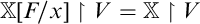


4.4 Properties of probabilistic teams
By simply replacing the symbol
 $\perp $
by the symbol
$\perp $
by the symbol
 $\mathbin {\perp \!\!\!\perp }$
, we get the probabilistic versions of the previously introduced possibilistic team properties of empirical and hidden-variable teams. These are in line with the definitions in [Reference Brandenburger and Yanofsky10], with the exception of no-signalling and parameter independence which suffer from the same weakness as their possibilistic counterparts and which we have generalized here.
$\mathbin {\perp \!\!\!\perp }$
, we get the probabilistic versions of the previously introduced possibilistic team properties of empirical and hidden-variable teams. These are in line with the definitions in [Reference Brandenburger and Yanofsky10], with the exception of no-signalling and parameter independence which suffer from the same weakness as their possibilistic counterparts and which we have generalized here.
Definition 4.26 (Probabilistic Team Properties)
-
(i) A probabilistic empirical team
$\mathbb {X}$
supports probabilistic no-signalling if it satisfies the formula (PNS)
$$ \begin{align} \bigwedge_{I\subseteq n}\{x_i \mid i\notin I\}\mathbin{\perp\!\!\!\perp}_{\{x_i \mid i\in I\}\vec z}\{y_i \mid i\in I\}. \end{align} $$
-
(ii) A probabilistic hidden-variable team
$\mathbb {X}$
supports probabilistic weak determinism if it satisfies the formula (PWD)
$$ \begin{align} \bigwedge_{i<n} \mathop{=}\hspace{-0.7pt}({\vec{x}\vec{z}},y_i). \end{align} $$
-
(iii) A probabilistic hidden-variable team
$\mathbb {X}$
supports probabilistic strong determinism if it satisfies the formula (PSD)
$$ \begin{align} \bigwedge_{i<n} \mathop{=}\hspace{-0.7pt}({x_i\vec{z}},y_i). \end{align} $$
-
(iv) A probabilistic hidden-variable team
$\mathbb {X}$
supports probabilistic single-valuedness if it satisfies the formula (PSV)
$$ \begin{align} \mathop{=}\hspace{-0.7pt}(\vec{z}). \end{align} $$
-
(v) A probabilistic hidden-variable team
$\mathbb {X}$
supports probabilistic
${\vec {z}}$
-independence if it satisfies the formula (PzI)
$$ \begin{align} \vec{z}\mathbin{\perp\!\!\!\perp}\vec{x}. \end{align} $$
-
(vi) A probabilistic hidden-variable team
$\mathbb {X}$
supports probabilistic parameter independence if it satisfies the formula (PPI)
$$ \begin{align} \bigwedge_{I\subseteq n}\{x_i \mid i\notin I\}\mathbin{\perp\!\!\!\perp}_{\{x_i \mid i\in I\}\vec z}\{y_i \mid i\in I\}. \end{align} $$
-
(vii) A probabilistic hidden-variable team
$\mathbb {X}$
supports probabilistic outcome independence if it satisfies the formula (POI)
$$ \begin{align} \bigwedge_{i<n} y_i\mathbin{\perp\!\!\!\perp}_{\vec{x}\vec{z}}\{y_j \mid j\neq i\}. \end{align} $$


As we did not have a syntactic formula for locality, we need to give an explicit semantic definition for probabilistic locality as well.
-
(viii) A probabilistic hidden-variable team
$\mathbb {X}$
supports probabilistic locality if for all
$\vec {a}$
,
$\vec {b}$
, and
$\vec {\gamma }$
, we have
$$\begin{align*}\left| \mathbb{X}_{\vec{x}\vec{y}\vec{z}=\vec{a}\vec{b}\vec{\gamma}} \right|\prod_{i<n}\left| \mathbb{X}_{x_i\vec{z} = a_i \vec{\gamma}} \right| = \left| \mathbb{X}_{\vec{x}\vec{z}=\vec{a}\vec{\gamma}} \right|\prod_{i<n}\left| \mathbb{X}_{x_i y_i \vec{z} = a_i b_i \vec{\gamma}} \right|. \end{align*}$$


Lemma 3.16, stating that locality is equivalent to the conjunction of parameter and outcome independence, remains true in the probabilistic world, at least with the simpler definition of parameter independence from [Reference Brandenburger and Yanofsky10].
Lemma 4.27. Probabilistic locality is equivalent to the formula
 $$\begin{align*}\bigwedge_{i<n}\left(\{ x_j \mid j\neq i \}\mathbin{\perp\!\!\!\perp}_{x_i\vec{z}}y_i \land y_i\mathbin{\perp\!\!\!\perp}_{\vec{x}\vec{z}}\{y_j \mid j\neq i\}\right)\!. \end{align*}$$
Proof Essentially proved in [Reference Brandenburger and Yanofsky10].
We conjecture that even with the more general definition of parameter independence, probabilistic locality is equivalent to the conjunction of probabilistic parameter independence and probabilistic outcome independence, as it is in the possibilistic case.
Corollary 4.28. For any of the properties in Definition 4.26, if a probabilistic team supports it, then the possibilistic collapse supports the corresponding possibilistic property.
Proof An immediate consequence of Proposition 4.10.
As by Proposition 4.25, the axioms presented in Section 2.2 are valid also in the probabilistic setting, all the results from Section 3.4 that were proved from the axioms are true also for probabilistic teams.
Corollary 4.29. The following hold for probabilistic teams (and more generally for K-teams whenever K is a commutative, positive, and multiplicatively cancellative semiring):
-
(i)
$\mathop {=}\hspace {-0.7pt}(\vec {x}\vec {z},\vec {y})\models \bigwedge _{i<n}y_i\mathbin {\perp \!\!\!\perp }_{\vec {x}\vec {z}}\{y_j \mid j\neq i\}$
, -
(ii)
$\mathop {=}\hspace {-0.7pt}(x_i\vec {z},y_i)\models \{x_j \mid j\neq i\}\mathbin {\perp \!\!\!\perp }_{x_i\vec {z}}y_i$
, -
(iii)
$\bigwedge _{i<n}\{x_j \mid j\neq i\}\mathbin {\perp \!\!\!\perp }_{x_i\vec {z}}y_i\land \mathop {=}\hspace {-0.7pt}(\vec {x}\vec {z},\vec {y})\ \models \ \bigwedge \mathop {=}\hspace {-0.7pt}(x_i\vec {z},y_i)$
, -
(iv)
$\varphi \models \exists z_0\dots \exists z_{l-1}(\mathop {=}\hspace {-0.7pt}(\vec {z})\land \varphi )$
. -
(v) The following formulas are equivalent:
-
(a)
$\bigwedge _{i<n}\{x_j \mid j\neq i\}\mathbin {\perp \!\!\!\perp }_{x_i} y_i$
, -
(b)
$\tilde \exists z_0\exists z_1\dots \exists z_{l-1} \left ( \vec {z}\mathbin {\perp \!\!\!\perp }\vec {x} \land \bigwedge _{i<n} \{ x_j \mid j\neq i \}\mathbin {\perp \!\!\!\perp }{x_i\vec {z}}y_i \right )$
.
-
-
(vi) The following formulas are equivalent:
-
(a)
$\bigwedge _{I\subseteq n}\{x_i \mid i\notin I\}\mathbin {\perp \!\!\!\perp }_{\{x_i\mid i\in I\}}\{y_i \mid i\in I\}$
, -
(b)
$\tilde {\exists }z_0\exists z_1\dots \exists z_{l-1} ( \vec {z}\mathbin {\perp \!\!\!\perp }\vec {x} \land \bigwedge _{I\subseteq n} \{x_i \mid i\notin I\}$
$\mathbin {\perp \!\!\!\perp }_{\{x_i\mid i\in I\}\vec {z}}\{y_i\mid i\in I\} )$
.
-


The above (i)–(vi) may seem like somewhat arbitrary observations. However, let us recall that they arise from examples motivated by quantum mechanics and each one of them has an intuitive interpretation in physics. It would seem more satisfactory to present a systematic study of such logical consequences and equivalences but we have already observed that it would be a formidable task bordering the impossible.
4.5 Building probabilistic teams
As we saw in Section 4.4, properties of probabilistic teams are inherited by their possibilistic collapses. Here we prove results concerning the question to what extent the converse holds: when can one construct a probabilistic team out of a possibilistic one, with the same properties?
Following [Reference Abramsky1], we proceed to show that some no-signalling teams have no probabilistic realization that would also support probabilistic no-signalling.
This also shows that
 $\varphi \models {\mathsf {P}\hspace {-0.5pt}\mathsf {R}}\varphi $
is not true for all formulas
$\varphi \models {\mathsf {P}\hspace {-0.5pt}\mathsf {R}}\varphi $
is not true for all formulas
 $\varphi $
of independence logic.
$\varphi $
of independence logic.
Proposition 4.30. Suppose that
 $n=2$
. There is an empirical team X supporting no-signalling such that there is no probabilistic team
$n=2$
. There is an empirical team X supporting no-signalling such that there is no probabilistic team
 $\mathbb {X}$
that supports probabilistic no-signalling and whose possibilistic collapse is X, i.e.,
$\mathbb {X}$
that supports probabilistic no-signalling and whose possibilistic collapse is X, i.e.,
 $$\begin{align*}\bigwedge_{i<n}\{x_j \mid j\neq i\}\perp_{x_i}y_i\ \not\models\ {\mathsf{P}\hspace{-0.5pt}\mathsf{R}}\bigwedge_{i<n}\{x_j \mid j\neq i\}\perp_{x_i}y_i. \end{align*}$$
Proof We let
 $X = \{s_0,\dots ,s_{11}\}$
, where the assignments
$X = \{s_0,\dots ,s_{11}\}$
, where the assignments
 $s_i$
are as follows:
$s_i$
are as follows:

It is straightforward to check that X supports no-signalling. Suppose for a contradiction that
 $\mathbb {X}$
is a probabilistic team that supports probabilistic no-signalling and whose possibilistic collapse is X. Then there are positive numbers
$\mathbb {X}$
is a probabilistic team that supports probabilistic no-signalling and whose possibilistic collapse is X. Then there are positive numbers
 $p_0,\dots ,p_{11}$
with
$p_0,\dots ,p_{11}$
with
 $\sum _{i<12}p_i = 1$
such that
$\sum _{i<12}p_i = 1$
such that
 $\mathbb {X}(s_i)=p_i$
for all
$\mathbb {X}(s_i)=p_i$
for all
 $i<12$
. By probabilistic no-signalling,
$i<12$
. By probabilistic no-signalling,
 $$\begin{align*}\mathbb{X}\models x_{1-i}\mathbin{\perp\!\!\!\perp}_{x_i} y_i, \end{align*}$$
for all
 $i\in \{0,1\}$
, so we have, for all
$i\in \{0,1\}$
, so we have, for all
 $a,b,c,i\in \{0,1\}$
,
$a,b,c,i\in \{0,1\}$
,
 $$\begin{align*}\left| \mathbb{X}_{x_{1-i} x_i = ab} \right|\cdot\left| \mathbb{X}_{x_i y_i = bc} \right| = \left| \mathbb{X}_{x_{1-i} x_i y_i = abc} \right|\cdot\left| \mathbb{X}_{x_i=b} \right|. \end{align*}$$
Calculating the marginal probabilities and applying the above condition, we get the following four equations:
-
(i)
$p_2 p_3 = (p_0 + p_1)(p_4 + p_5)$
, -
(ii)
$p_0 p_8 = (p_1 + p_2)(p_6 + p_7)$
, -
(iii)
$p_6 p_{11} = (p_7 + p_8)(p_9 + p_{10})$
, and -
(iv)
$p_5 p_9 = (p_3 + p_4)(p_{10} + p_{11})$
.


From this, using the third and the fourth equations, we get
 $$\begin{align*}p_6 p_{11} p_5 p_9 = (p_7 + p_8)(p_9 + p_{10})(p_3 + p_4)(p_{10} + p_{11})> p_8 p_9 p_3 p_{11}, \end{align*}$$
whence
 $p_5 p_6> p_3 p_8$
. Then by multiplying by
$p_5 p_6> p_3 p_8$
. Then by multiplying by
 $p_2$
and using the first equation, we get
$p_2$
and using the first equation, we get
 $$\begin{align*}p_2 p_5 p_6> p_2 p_3 p_8 = (p_0 + p_1)(p_4 + p_5)p_8 > p_0 p_5 p_8, \end{align*}$$
whence
 $p_2 p_6> p_0 p_8$
. Then finally, using the second equation, we get
$p_2 p_6> p_0 p_8$
. Then finally, using the second equation, we get
 $$\begin{align*}p_2 p_6> p_0 p_8 = (p_1 + p_2)(p_6 + p_7) > p_2 p_6, \end{align*}$$
which is a contradiction.
A minimal example of a possibilistic no-signalling team which is not a collapse of any probabilistic no-signalling team can be obtained by translating an example of [Reference Abramsky, Barbosa, Kishida, Lal and Mansfield2]—which occurs as part of a discussion about the question whether there exists an intrinsic characterization of the class of no-signalling teams that are collapses of probabilistic no-signalling teams—into our team-semantic framework.
The next property of empirical and hidden-variable teams, measurement locality, was introduced by the first author in [Reference Abramsky1]. Measurement locality states that the measurement variables are mutually independent of each other.
Definition 4.31 (Measurement Locality)
An empirical team X supports measurement locality if it satisfies the formula
 $$ \begin{align} \bigwedge_{i<n} x_i\perp\{x_j \mid j\neq i\}. \end{align} $$
A hidden-variable team X supports measurement locality if it satisfies the formula
 $$ \begin{align} \bigwedge_{i<n} x_i\perp_{\vec{z}}\{x_j \mid j\neq i\}. \end{align} $$
Definition 4.32 (Probabilistic Measurement Locality)
A probabilistic empirical team
 $\mathbb {X}$
supports probabilistic measurement locality if it satisfies the formula
$\mathbb {X}$
supports probabilistic measurement locality if it satisfies the formula
 $$ \begin{align} \bigwedge_{i<n} x_i\mathbin{\perp\!\!\!\perp}\{x_j \mid j\neq i\}. \end{align} $$
A probabilistic hidden-variable team
 $\mathbb {X}$
supports probabilistic measurement locality if it satisfies the formula
$\mathbb {X}$
supports probabilistic measurement locality if it satisfies the formula
 $$ \begin{align} \bigwedge_{i<n} x_i\mathbin{\perp\!\!\!\perp}_{\vec{z}}\{x_j \mid j\neq i\}. \end{align} $$
Corollary 4.33. Whenever a probabilistic team supports probabilistic measurement locality, the possibilistic collapse supports measurement locality.
Proof An immediate consequence of Proposition 4.10.
Definition 4.34. Given sets
 $A=\prod _{i<n}A_i$
and
$A=\prod _{i<n}A_i$
and
 $B=\prod _{i<n}B_i$
and a probability distribution
$B=\prod _{i<n}B_i$
and a probability distribution
 $p_{\vec {a}}$
on B for each
$p_{\vec {a}}$
on B for each
 $\vec {a}\in A$
, we say that a probabilistic empirical team
$\vec {a}\in A$
, we say that a probabilistic empirical team
 $\mathbb {X}$
is a uniform joint distribution of the outcome distribution family
$\mathbb {X}$
is a uniform joint distribution of the outcome distribution family
 $\{p_{\vec {a}} \mid \vec {a}\in A\}$
if the value domain of
$\{p_{\vec {a}} \mid \vec {a}\in A\}$
if the value domain of
 $\mathbb {X}$
is
$\mathbb {X}$
is
 $\bigcup _{i<n}(A_i\cup B_i)$
and
$\bigcup _{i<n}(A_i\cup B_i)$
and
 $\mathbb {X}(s) = p_{s(\vec {x})}(s(\vec {y}))/\left | A \right |$
whenever
$\mathbb {X}(s) = p_{s(\vec {x})}(s(\vec {y}))/\left | A \right |$
whenever
 $s(x_i)\in A_i$
and
$s(x_i)\in A_i$
and
 $s(y_i)\in B_i$
for all
$s(y_i)\in B_i$
for all
 $i<n$
, and
$i<n$
, and
 $\mathbb {X}(s)=0$
otherwise.
$\mathbb {X}(s)=0$
otherwise.
Similarly, given a set
 $\Gamma $
of possible hidden-variable values and outcome distributions
$\Gamma $
of possible hidden-variable values and outcome distributions
 $p_{\vec {a}\vec {\gamma }}$
on B for
$p_{\vec {a}\vec {\gamma }}$
on B for
 $\vec {a}\in A$
and
$\vec {a}\in A$
and
 $\vec {\gamma }\in \Gamma $
, we say that a probabilistic hidden-variable team
$\vec {\gamma }\in \Gamma $
, we say that a probabilistic hidden-variable team
 $\mathbb {X}$
is a uniform joint distribution of the outcome distribution family if
$\mathbb {X}$
is a uniform joint distribution of the outcome distribution family if
 $X(s)=p_{s(\vec {x}\vec {z})}(s(\vec {y}))/\left | A\times \Gamma \right |$
.
$X(s)=p_{s(\vec {x}\vec {z})}(s(\vec {y}))/\left | A\times \Gamma \right |$
.
Proposition 4.35. A uniform joint distribution of an outcome distribution family supports probabilistic measurement locality.
Proof First observe that
 $$ \begin{align*} \left| \mathbb{X}_{x_i\vec{z} = a_i\vec{\gamma}} \right| &= \sum_{\substack{\vec{c}\in A \\ c_i=a_i}}\sum_{\vec{b}\in B}\frac{p_{\vec{c}\vec{\gamma}}(\vec{b})}{\left| A\times\Gamma \right|} = \sum_{\substack{\vec{c}\in A \\ c_i=a_i}}\frac{1}{\left| A \right|\left| \Gamma \right|} \\ &= \frac{1}{\left| A \right|\left| \Gamma \right|}\left| \{\vec{c}\in A \mid c_i=a_i\} \right| \\ &= \frac{1}{\left| \Gamma \right|\prod_{j<n}\left| A_j \right|}\prod_{\substack{j<n \\ j\neq i}}\left| A_j \right| \\ &= \frac{1}{\left| \Gamma \right|\left| A_i \right|}. \end{align*} $$
Then we have
 $$ \begin{align*} \left| \mathbb{X}_{\vec{x}\vec{z} = \vec{a}\vec{\gamma}} \right|\cdot\left| \mathbb{X}_{\vec{z}=\vec{\gamma}} \right|^{n-1} &= \left( \sum_{\vec{b}\in B} \frac{p_{\vec{a}\vec{\gamma}}(\vec{b})}{\left| A\times\Gamma \right|} \right)\left( \sum_{\vec{c}\in A}\sum_{\vec{b}\in B}\frac{p_{\vec{c}\vec{\gamma}}(\vec{b})}{\left| A\times\Gamma \right|} \right)^{n-1} \\ &= \frac{1}{\left| A \right|\left| \Gamma \right|}\left( \sum_{\vec{c}\in A}\frac{p_{\vec{c}\vec{\gamma}}(\vec{b})}{\left| A \right|\left| \Gamma \right|} \right)^{n-1} = \frac{1}{\left| A \right|\left| \Gamma \right|}\cdot\left( \frac{\left| A \right|}{\left| A \right|\left| \Gamma \right|} \right)^{n-1} \\ &= \frac{1}{\left| A \right|\left| \Gamma \right|{}^n} = \frac{1}{\left| \Gamma \right|{}^n}\prod_{i<n}\frac{1}{\left| A_i \right|} = \prod_{i<n}\frac{1}{\left| \Gamma \right|\left| A_i \right|} \\ &= \prod_{i<n}\left| \mathbb{X}_{x_i{\vec{z}} = a_i\vec\gamma} \right|. \end{align*} $$
Now we observe the following fact that is easy to prove by induction on n: a probabilistic team
 $\mathbb {Y}$
satisfies the formula
$\mathbb {Y}$
satisfies the formula
 $\bigwedge _{i<n} v_i\mathbin {\perp \!\!\!\perp }_{\vec {u}}\{v_j \mid j\neq i\}$
if and only if for all
$\bigwedge _{i<n} v_i\mathbin {\perp \!\!\!\perp }_{\vec {u}}\{v_j \mid j\neq i\}$
if and only if for all
 $\vec {a}$
and
$\vec {a}$
and
 $\vec {b}$
,
$\vec {b}$
,
 $$\begin{align*}\left| \mathbb{Y}_{\vec{v}\vec{u}=\vec{a}\vec{b}} \right|\cdot\left| \mathbb{Y}_{\vec{u}=\vec{b}} \right|{}^{n-1} = \prod_{i<n}\left| \mathbb{Y}_{v_i \vec{u} = a_i \vec{b}} \right|. \end{align*}$$
Each
 $v_i$
can also be replaced by a tuple of variables. From this and the above calculations, it follows that
$v_i$
can also be replaced by a tuple of variables. From this and the above calculations, it follows that
 $\mathbb {X}\models x_i\mathbin {\perp \!\!\!\perp }_{\vec {z}}\{x_j \mid j\neq i\}$
.
$\mathbb {X}\models x_i\mathbin {\perp \!\!\!\perp }_{\vec {z}}\{x_j \mid j\neq i\}$
.
Next we show that there is a canonical way of constructing a probabilistic team out of a possibilistic hidden-variable team that supports
 ${\vec {z}}$
-independence, and that such a probabilistic team will support locality, measurement locality, and
${\vec {z}}$
-independence, and that such a probabilistic team will support locality, measurement locality, and
 ${\vec {z}}$
-independence if its possibilistic collapse does.
${\vec {z}}$
-independence if its possibilistic collapse does.
Definition 4.36. Given a hidden-variable team X that supports
 ${\vec {z}}$
-independence, we define the probabilistic hidden-variable team
${\vec {z}}$
-independence, we define the probabilistic hidden-variable team
 $\mathop {\mathrm {Prob}\!}\left ( X \right )$
as follows. Denote
$\mathop {\mathrm {Prob}\!}\left ( X \right )$
as follows. Denote
 $$ \begin{align*} \Gamma &= \{ s(\vec{z}) \mid s\in X \}, \\ M &= \{ s(\vec{x}) \mid s\in X \}, \\ O_{\vec{a},\vec{\gamma}} &= \{ s(\vec{y}) \mid s\in X, s(\vec{x}\vec{z}) = \vec{a}\vec{\gamma} \}, \end{align*} $$
 $m_{\mathrm {h}} = \left | \Gamma \right |$
,
$m_{\mathrm {h}} = \left | \Gamma \right |$
,
 $m_{\mathrm {m}} = \left | M \right |$
, and
$m_{\mathrm {m}} = \left | M \right |$
, and
 $m_{\mathrm {o}}(\vec {a},\vec {\gamma }) = \left | O_{\vec {a},\vec {\gamma }} \right |$
. We then define
$m_{\mathrm {o}}(\vec {a},\vec {\gamma }) = \left | O_{\vec {a},\vec {\gamma }} \right |$
. We then define
 $\mathop {\mathrm {Prob}\!}\left ( X \right )$
by setting
$\mathop {\mathrm {Prob}\!}\left ( X \right )$
by setting
 $$\begin{align*}\mathop{\mathrm{Prob}\!}\left( X \right)(s) = \begin{cases} \displaystyle\frac{1}{m_{\mathrm{h}}\cdot m_{\mathrm{m}}\cdot m_{\mathrm{o}}(s(\vec{x}),s(\vec{z}))} & \text{if } s(\vec{x})\in M \text{ and } s(\vec{z})\in\Gamma, \\ 0 & \text{otherwise}. \end{cases} \end{align*}$$
Lemma 4.37.
 $\mathop {\mathrm {Prob}\!}\left ( X \right )$
is well-defined and
$\mathop {\mathrm {Prob}\!}\left ( X \right )$
is well-defined and
 $\operatorname {\mathrm {supp}}\mathop {\mathrm {Prob}\!}\left ( X \right ) = X$
.
$\operatorname {\mathrm {supp}}\mathop {\mathrm {Prob}\!}\left ( X \right ) = X$
.
Proof First, as X supports
 ${\vec {z}}$
-independence, for every
${\vec {z}}$
-independence, for every
 $s,s'\in X$
we can find
$s,s'\in X$
we can find
 $s"\in X$
with
$s"\in X$
with
 $s"(\vec {x})=s(\vec {x})$
and
$s"(\vec {x})=s(\vec {x})$
and
 $s"(\vec {z})=s'(\vec {z})$
, and thus, given an assignment s, the condition
$s"(\vec {z})=s'(\vec {z})$
, and thus, given an assignment s, the condition
 $$\begin{align*}s(\vec{x})\in M \text{ and } s(\vec{z})\in\Gamma \end{align*}$$
implies that there is some
 $s'\in X$
with
$s'\in X$
with
 $s'(\vec {x}\vec {z})=s(\vec {x}\vec {z})$
and thus the number
$s'(\vec {x}\vec {z})=s(\vec {x}\vec {z})$
and thus the number
 $m_{\mathrm {o}}(s(\vec {x}),s(\vec {z}))$
is non-zero. Hence
$m_{\mathrm {o}}(s(\vec {x}),s(\vec {z}))$
is non-zero. Hence
 $\mathop {\mathrm {Prob}\!}\left ( X \right )$
is well-defined as a function. What is left to show is that
$\mathop {\mathrm {Prob}\!}\left ( X \right )$
is well-defined as a function. What is left to show is that
 $\mathop {\mathrm {Prob}\!}\left ( X \right )$
is a probability distribution. Let us notice that for each
$\mathop {\mathrm {Prob}\!}\left ( X \right )$
is a probability distribution. Let us notice that for each
 $\vec {a}\vec {b}\vec {\gamma }$
, the probability of the assignment
$\vec {a}\vec {b}\vec {\gamma }$
, the probability of the assignment
 $\vec {x}\vec {y}\vec {z}\mapsto \vec {a}\vec {b}\vec {\gamma }$
does not depend on
$\vec {x}\vec {y}\vec {z}\mapsto \vec {a}\vec {b}\vec {\gamma }$
does not depend on
 $\vec {b}$
, so each assignment s with
$\vec {b}$
, so each assignment s with
 $s(\vec {x}\vec {z})=\vec {a}\vec {\gamma }$
has an equal probability, which is
$s(\vec {x}\vec {z})=\vec {a}\vec {\gamma }$
has an equal probability, which is
 $1/(m_{\mathrm {h}}m_{\mathrm {m}}m_{\mathrm {o}}(\vec {a},\vec {\gamma }))$
, and thus the joint probability of such assignments is
$1/(m_{\mathrm {h}}m_{\mathrm {m}}m_{\mathrm {o}}(\vec {a},\vec {\gamma }))$
, and thus the joint probability of such assignments is
 $$ \begin{align*} \left| \mathop{\mathrm{Prob}\!}\left( X \right)_{\vec{x}\vec{z}=\vec{a}\vec{\gamma}} \right| &= \sum_{\vec{b}}\mathop{\mathrm{Prob}\!}\left( X \right)(\vec{x}\vec{y}\vec{z}\mapsto\vec{a}\vec{b}\vec{\gamma}) = \frac{m_{\mathrm{o}}(\vec{a},\vec{\gamma})}{m_{\mathrm{h}}m_{\mathrm{m}}m_{\mathrm{o}}(\vec{a},\vec{\gamma})} = \frac{1}{m_{\mathrm{h}}m_{\mathrm{m}}}. \end{align*} $$
This, in turn, does not depend on
 $\vec {a}$
or
$\vec {a}$
or
 $\vec {\gamma }$
. Also, by
$\vec {\gamma }$
. Also, by
 ${\vec {z}}$
-independence, we have
${\vec {z}}$
-independence, we have
 $\left | \{s \mid s(\vec {x}\vec {z}) = \vec {a}\vec {\gamma } \} \right | = m_{\mathrm {m}}\cdot m_{\mathrm {h}}$
. Thus
$\left | \{s \mid s(\vec {x}\vec {z}) = \vec {a}\vec {\gamma } \} \right | = m_{\mathrm {m}}\cdot m_{\mathrm {h}}$
. Thus
 $$ \begin{align*} \sum_{s\in X} \mathop{\mathrm{Prob}\!}\left( X \right)(s) &= \sum_{\vec{a}\vec{b}\vec{\gamma}} \mathop{\mathrm{Prob}\!}\left( X \right)(\vec{x}\vec{y}\vec{z} \mapsto \vec{a}\vec{b}\vec{\gamma}) \\ &= \sum_{\vec{a}\vec{\gamma}} \frac{1}{m_{\mathrm{h}}m_{\mathrm{m}}} = m_{\mathrm{m}}m_{\mathrm{h}}\cdot\frac{1}{m_{\mathrm{h}}m_{\mathrm{m}}} = 1. \end{align*} $$
Thus
 $\mathop {\mathrm {Prob}\!}\left ( X \right )$
is a well-defined distribution. Clearly the collapse of
$\mathop {\mathrm {Prob}\!}\left ( X \right )$
is a well-defined distribution. Clearly the collapse of
 $\mathop {\mathrm {Prob}\!}\left ( X \right )$
is X.
$\mathop {\mathrm {Prob}\!}\left ( X \right )$
is X.
In contrast to Proposition 4.30, we now obtain the following proposition.
Proposition 4.38. Let X be a hidden-variable team supporting measurement locality,
 ${\vec {z}}$
-independence, and locality. Then
${\vec {z}}$
-independence, and locality. Then
 $\mathop {\mathrm {Prob}\!}\left ( X \right )$
supports probabilistic measurement locality, probabilistic
$\mathop {\mathrm {Prob}\!}\left ( X \right )$
supports probabilistic measurement locality, probabilistic
 ${\vec {z}}$
-independence, and probabilistic locality whose possibilistic collapse is X. Thus, the formula
${\vec {z}}$
-independence, and probabilistic locality whose possibilistic collapse is X. Thus, the formula

satisfies
 $\varphi \models {\mathsf {P}\hspace {-0.5pt}\mathsf {R}}\varphi $
.
$\varphi \models {\mathsf {P}\hspace {-0.5pt}\mathsf {R}}\varphi $
.
Proof Essentially proved in [Reference Abramsky1].
5 Empirical teams arising from quantum mechanics
A team, even what we call an empirical team, is in itself just an abstract set of assignments. It does not need to have any “provenance”, although in practical applications, teams arise from concrete data. In our current context of quantum mechanics, we use the abstract concept of a team for implications which indeed are totally general and abstract. However, when it comes to counter-examples demonstrating that some implications are not valid, the question arises whether our example teams are “merely” abstract or whether they can actually arise in experiments. One of the beauties of quantum physics is that we have a precise mathematical axiomatization of quantum mechanics, essentially due to von Neumann [Reference Von Neumann48]. This axiomatization is formulated in terms of operators on complex Hilbert spaces. We shall limit our discussion to the finite-dimensional case, where operators can be represented as complex matrices.
Definition 5.1. Let M and O be sets of n-tuples (the “set of measurements” and the “set of outcomes”), and, for
 $i<n$
, denote
$i<n$
, denote
 ${M_i = \{a_i \mid \vec {a}\in M \}}$
and
${M_i = \{a_i \mid \vec {a}\in M \}}$
and
 $O_i = \{ b_i \mid \vec {b}\in O \}$
. A finite-dimensional tensor-product quantum system of type
$O_i = \{ b_i \mid \vec {b}\in O \}$
. A finite-dimensional tensor-product quantum system of type
 $(M,O)$
is a tuple
$(M,O)$
is a tuple
where
-
•
$\mathcal {H}$
is the tensor product
$\bigotimes _{i<n}\mathcal {H}_i$
of finite-dimensional complex Hilbert spaces
$\mathcal {H}_i$
,
$i<n$
, -
• for all
$i<n$
and
$a\in M_i$
,
$\{A_i^{a,b} \mid b\in O_i \}$
is a positive operator-valued measure (POVM)Footnote
8
on
$\mathcal {H}_i$
, and -
•
$\rho $
is a density operator on
$\mathcal {H}$
(the “state of
$\mathcal {S}$
”), i.e., where
$$\begin{align*}\rho = \sum_{j<k}p_j\left| \psi_j \right\rangle\left\langle \psi_j \right|, \end{align*}$$
$\left | \psi _j \right \rangle \in \mathcal {H}$
and
$p_j\in [0,1]$
for all
$j<k$
and
$\sum _{j<k}p_j = 1$
.


For each measurement
 $\vec {a}\in M$
, we define the probability distribution
$\vec {a}\in M$
, we define the probability distribution
 $p^{\mathcal {S}}_{\vec {a}}$
of outcomes by setting
$p^{\mathcal {S}}_{\vec {a}}$
of outcomes by setting ![]() , where
, where
 $\operatorname {\mathrm {Tr}}(L)$
denotes the trace of the matrix L.
$\operatorname {\mathrm {Tr}}(L)$
denotes the trace of the matrix L.
Definition 5.2. Let
 $\mathbb {X}$
be a probabilistic team with variable domain
$\mathbb {X}$
be a probabilistic team with variable domain
 $V_{\text {m}}\cup V_{\text {o}}$
. Denote
$V_{\text {m}}\cup V_{\text {o}}$
. Denote
 $M = \{s(\vec {x}) \mid s\in \operatorname {\mathrm {supp}}\mathbb {X} \}$
and
$M = \{s(\vec {x}) \mid s\in \operatorname {\mathrm {supp}}\mathbb {X} \}$
and
 $O = \{s(\vec {y}) \mid s\in \operatorname {\mathrm {supp}}\mathbb {X} \}$
.
$O = \{s(\vec {y}) \mid s\in \operatorname {\mathrm {supp}}\mathbb {X} \}$
.
We say that
 $\mathbb {X}$
is a finite-dimensional tensor-product quantum-mechanical team if there exists a finite-dimensional tensor-product quantum system
$\mathbb {X}$
is a finite-dimensional tensor-product quantum-mechanical team if there exists a finite-dimensional tensor-product quantum system
 $\mathcal {S}$
of type
$\mathcal {S}$
of type
 $(M,O)$
such that for all assignments s, we have
$(M,O)$
such that for all assignments s, we have
 $$\begin{align*}\mathbb{X}(s)=p^{\mathcal{S}}_{s(\vec{x})}(s(\vec{y}))/\left| M \right|. \end{align*}$$
We call an empirical probabilistic team
 $\mathbb {X}$
a finite-dimensional tensor-product quantum-mechanical realization of an empirical possibilistic team X if X is the possibilistic collapse of
$\mathbb {X}$
a finite-dimensional tensor-product quantum-mechanical realization of an empirical possibilistic team X if X is the possibilistic collapse of
 $\mathbb {X}$
and
$\mathbb {X}$
and
 $\mathbb {X}$
is finite-dimensional tensor-product quantum-mechanical.
$\mathbb {X}$
is finite-dimensional tensor-product quantum-mechanical.
Denote by
 $\mathrm {QT}$
the set of finite-dimensional tensor-product quantum-mechanically realizable teams.
$\mathrm {QT}$
the set of finite-dimensional tensor-product quantum-mechanically realizable teams.
We can define a new atomic formula
 ${\mathsf {Q}\hspace {-0.5pt}\mathsf {R}}$
such that
${\mathsf {Q}\hspace {-0.5pt}\mathsf {R}}$
such that
 $X\models {\mathsf {Q}\hspace {-0.5pt}\mathsf {R}}$
if X has a finite-dimensional tensor-product quantum realization. In other words,
$X\models {\mathsf {Q}\hspace {-0.5pt}\mathsf {R}}$
if X has a finite-dimensional tensor-product quantum realization. In other words,
 $X\models {\mathsf {Q}\hspace {-0.5pt}\mathsf {R}}$
if and only if
$X\models {\mathsf {Q}\hspace {-0.5pt}\mathsf {R}}$
if and only if
 $X\in \mathrm {QT}$
. Then one can ask what kind of properties this atom has. More generally, we can define an operation
$X\in \mathrm {QT}$
. Then one can ask what kind of properties this atom has. More generally, we can define an operation
 ${\mathsf {Q}\hspace {-0.5pt}\mathsf {R}}$
by
${\mathsf {Q}\hspace {-0.5pt}\mathsf {R}}$
by
 $X\models {\mathsf {Q}\hspace {-0.5pt}\mathsf {R}}\varphi $
if X has a finite-dimensional tensor-product quantum-mechanical realization
$X\models {\mathsf {Q}\hspace {-0.5pt}\mathsf {R}}\varphi $
if X has a finite-dimensional tensor-product quantum-mechanical realization
 $\mathbb {X}$
such that
$\mathbb {X}$
such that
 $\mathbb {X}\models \varphi $
, analogously to the operation
$\mathbb {X}\models \varphi $
, analogously to the operation
 ${\mathsf {P}\hspace {-0.5pt}\mathsf {R}}$
.
${\mathsf {P}\hspace {-0.5pt}\mathsf {R}}$
.
One can also ask what kind of property of probabilistic teams being finite-dimensional tensor-product quantum-mechanical is. In [Reference Durand, Hannula, Kontinen, Meier, Virtema, Ferrarotti and Woltran15], Durand et al. showed that probabilistic independence logic (with rational probabilities) is equivalent to a probabilistic variant of existential second-order logic
 $\mathrm {ESOf}_{\mathbb {Q}}$
. Is being finite-dimensional tensor-product quantum-mechanical expressible in
$\mathrm {ESOf}_{\mathbb {Q}}$
. Is being finite-dimensional tensor-product quantum-mechanical expressible in
 $\mathrm {ESOf}_{\mathbb {R}}$
or do we need more expressivity?
$\mathrm {ESOf}_{\mathbb {R}}$
or do we need more expressivity?
We now observe that the set
 $\mathrm {QT} = \{X \mid X\models {\mathsf {Q}\hspace {-0.5pt}\mathsf {R}}\}$
is undecidable but recursively enumerable. For this purpose, we briefly introduce non-local games and then apply a result of Slofstra [Reference Slofstra43].
$\mathrm {QT} = \{X \mid X\models {\mathsf {Q}\hspace {-0.5pt}\mathsf {R}}\}$
is undecidable but recursively enumerable. For this purpose, we briefly introduce non-local games and then apply a result of Slofstra [Reference Slofstra43].
-
(i) Let
$I_{\mathrm {A}}$
,
$I_{\mathrm{B}} $
,
$O_{\mathrm {A}}$
, and
$O_{\mathrm{B}} $
be finite sets and let
$V\colon O_{\mathrm {A}}\times O_{\mathrm{B}} \times I_{\mathrm {A}}\times I_{\mathrm{B}} \to \{0,1\}$
be a functionFootnote
9
. A (two-player one-round) non-local game G with question sets
$I_{\mathrm {A}}$
and
$I_{\mathrm{B}} $
, answer sets
$O_{\mathrm {A}}$
and
$O_{\mathrm{B}} $
, and decision predicate V is defined as follows: the first player (Alice) receives an element
$c\in I_{\mathrm {A}}$
and the second player (Bob) receives an element
$d\in I_{\mathrm{B}} $
. Alice returns an element
$a\in O_{\mathrm {A}}$
and Bob returns an element
$b\in O_{\mathrm{B}} $
. The players are not allowed to communicate the received inputs or their chosen outcomes to each other. The players win if
$V(a,b\mid c,d)=1$
and lose otherwise. -
(ii) Let G be a non-local game. A strategy for G is a function
$p\colon O_{\mathrm {A}}\times O_{\mathrm{B}} \times I_{\mathrm {A}}\times I_{\mathrm{B}} \to [0,1]$
such that for each pair
$(c,d)\in I_{\mathrm {A}}\times I_{\mathrm{B}} $
the function
$(a,b)\mapsto p(a,b\mid c,d)$
is a probability distribution. A strategy p is perfect if
$V(a,b\mid c,d)=0$
implies
$p(a,b\mid c,d)=0$
. -
(iii) Let G be a non-local game and p a strategy for G. We say that p is a quantum strategy if there are finite-dimensional Hilbert spaces
$H_{\mathrm {A}}$
and
$H_{\mathrm{B}} $
, a quantum state
$\rho $
of
$H_{\mathrm {A}}\otimes H_{\mathrm{B}} $
, a POVM
$(M^c_a)_{a\in O_{\mathrm {A}}}$
on
$H_{\mathrm {A}}$
for each
$c\in I_{\mathrm {A}}$
, and a POVM
$(N^d_b)_{b\in O_{\mathrm{B}} }$
on
$H_{\mathrm{B}} $
for each
$d\in I_{\mathrm{B}} $
such that for all
$$\begin{align*}p(a,b\mid c,d) = \operatorname{\mathrm{Tr}}(M^c_a\otimes N^d_b\rho) \end{align*}$$
$(a,b,c,d)\in O_{\mathrm {A}}\times O_{\mathrm{B}} \times I_{\mathrm {A}}\times I_{\mathrm{B}} $
.


Theorem 5.4 (Slofstra [Reference Slofstra43])
It is undecidable to determine whether a non-local game has a perfect quantum strategy.
Proposition 5.5. There is a many-one reduction from non-local games that have a perfect quantum strategy to teams that have a finite-dimensional tensor-product quantum-mechanical realization.
Proof Let G be a game with question sets
 $I_{\mathrm {A}}$
and
$I_{\mathrm {A}}$
and
 $I_{\mathrm{B}} $
and answer sets
$I_{\mathrm{B}} $
and answer sets
 $O_{\mathrm {A}}$
and
$O_{\mathrm {A}}$
and
 $O_{\mathrm{B}} $
and decision predicate V. We may assume that for each
$O_{\mathrm{B}} $
and decision predicate V. We may assume that for each
 $c\in I_{\mathrm {A}}$
and
$c\in I_{\mathrm {A}}$
and
 $d\in I_{\mathrm{B}} $
there are some
$d\in I_{\mathrm{B}} $
there are some
 $a\in O_{\mathrm {A}}$
and
$a\in O_{\mathrm {A}}$
and
 $b\in O_{\mathrm{B}} $
such that
$b\in O_{\mathrm{B}} $
such that
 $V(a,b \mid c,d)=1$
; otherwise, we may just map G into the empty team. We let
$V(a,b \mid c,d)=1$
; otherwise, we may just map G into the empty team. We let
 $X_G$
be the set of all assignments s with domain
$X_G$
be the set of all assignments s with domain
 $\{x_0,x_1,y_0,y_1\}$
such that
$\{x_0,x_1,y_0,y_1\}$
such that
 $s(x_0)\in I_{\mathrm {A}}$
,
$s(x_0)\in I_{\mathrm {A}}$
,
 $s(x_1)\in I_{\mathrm{B}} $
,
$s(x_1)\in I_{\mathrm{B}} $
,
 $s(y_0)\in O_{\mathrm {A}}$
,
$s(y_0)\in O_{\mathrm {A}}$
,
 $s(y_1)\in O_{\mathrm{B}} $
, and
$s(y_1)\in O_{\mathrm{B}} $
, and
 $V(s(y_0),s(y_1) \mid s(x_0),s(x_1))=1$
. Let
$V(s(y_0),s(y_1) \mid s(x_0),s(x_1))=1$
. Let
 $M = I_{\mathrm {A}}\times I_{\mathrm{B}} $
and
$M = I_{\mathrm {A}}\times I_{\mathrm{B}} $
and
 $$ \begin{align*} O &= \{(a,b)\in O_{\mathrm{A}}\times O_{\mathrm{B}} \mid V(a,b \mid c,d)=1 \text{ for some } c\in I_{\mathrm{A}} \text{ and } d\in I_{\mathrm{B}} \}, \end{align*} $$
and denote by
 $M_0$
,
$M_0$
,
 $M_1$
,
$M_1$
,
 $O_0$
, and
$O_0$
, and
 $O_1$
the appropriate projections of M and O. Then
$O_1$
the appropriate projections of M and O. Then
 $M=\{s(x_0x_1) \mid s\in X_G\}$
and
$M=\{s(x_0x_1) \mid s\in X_G\}$
and
 $O=\{s(y_0y_1) \mid s\in X_G\}$
.
$O=\{s(y_0y_1) \mid s\in X_G\}$
.
We show that G has a perfect quantum strategy if and only if
 $X_G$
is realizable by a finite-dimensional tensor-product quantum-mechanical team. We only show one direction, the other is similar. Suppose that p is a perfect quantum strategy for G. Then there are finite-dimensional Hilbert spaces
$X_G$
is realizable by a finite-dimensional tensor-product quantum-mechanical team. We only show one direction, the other is similar. Suppose that p is a perfect quantum strategy for G. Then there are finite-dimensional Hilbert spaces
 $H_{\mathrm {A}}$
and
$H_{\mathrm {A}}$
and
 $H_{\mathrm{B}} $
, a quantum state
$H_{\mathrm{B}} $
, a quantum state
 $\rho $
of
$\rho $
of
 $H_{\mathrm {A}}\otimes H_{\mathrm{B}} $
, a POVM
$H_{\mathrm {A}}\otimes H_{\mathrm{B}} $
, a POVM
 $\{ M^c_a \mid a\in O_{\mathrm {A}} \}$
on
$\{ M^c_a \mid a\in O_{\mathrm {A}} \}$
on
 $H_{\mathrm {A}}$
for each
$H_{\mathrm {A}}$
for each
 $c\in I_{\mathrm {A}}$
, and a POVM
$c\in I_{\mathrm {A}}$
, and a POVM
 $\{ N^d_b \mid b\in O_{\mathrm{B}} \}$
on
$\{ N^d_b \mid b\in O_{\mathrm{B}} \}$
on
 $H_{\mathrm{B}} $
for each
$H_{\mathrm{B}} $
for each
 $d\in I_{\mathrm{B}} $
such that
$d\in I_{\mathrm{B}} $
such that
 $$\begin{align*}p(a,b\mid c,d)=\operatorname{\mathrm{Tr}}(M^c_a\otimes N^d_b\rho) \end{align*}$$
for all
 $(a,b,c,d)\in O_{\mathrm {A}}\times O_{\mathrm{B}} \times I_{\mathrm {A}}\times I_{\mathrm{B}} $
. We now define a quantum system
$(a,b,c,d)\in O_{\mathrm {A}}\times O_{\mathrm{B}} \times I_{\mathrm {A}}\times I_{\mathrm{B}} $
. We now define a quantum system
 $$\begin{align*}\mathcal{S}=(\mathcal{H}, (A^{c,a}_i)_{c\in M_i, a\in O_i, i<2},\rho) \end{align*}$$
of type
 $(M,O)$
by setting
$(M,O)$
by setting
-
•
$\mathcal {H} = \mathcal {H}_{\mathrm {A}}\otimes \mathcal {H}_{\mathrm{B}} $
, and -
•
$A^{c,a}_0 = M^c_a$
and
$A^{d,b}_1 = N^d_b$
for all
$a\in O_0$
,
$b\in O_1$
,
$c\in M_0$
and
$d\in M_1$
.


Now clearly
 $$ \begin{align*} p^{\mathcal{S}}_{(c,d)}(a,b) &= \operatorname{\mathrm{Tr}}(A^{(c,d),(a,b)}\rho) = \operatorname{\mathrm{Tr}}(M^c_a\otimes N^d_b\rho) = p(a,b \mid c,d). \end{align*} $$
As p is a perfect strategy, we have
 $p(a,b \mid c,d)=0$
for any a, b, c, and d such that
$p(a,b \mid c,d)=0$
for any a, b, c, and d such that
 $V(a,b \mid c,d)=0$
. Thus the probabilistic team
$V(a,b \mid c,d)=0$
. Thus the probabilistic team
 $\mathbb {X}$
arising from the quantum system
$\mathbb {X}$
arising from the quantum system
 $\mathcal {S}$
is such that
$\mathcal {S}$
is such that
 $\mathbb {X}(s)>0$
if and only if
$\mathbb {X}(s)>0$
if and only if
 $V(s(y_0),s(y_1) \mid s(x_0), s(x_1))=1$
. Hence the possibilistic collapse of
$V(s(y_0),s(y_1) \mid s(x_0), s(x_1))=1$
. Hence the possibilistic collapse of
 $\mathbb {X}$
is
$\mathbb {X}$
is
 $X_G$
, and thus
$X_G$
, and thus
 $\mathbb {X}$
is a finite-dimensional tensor-product quantum-mechanical realization of
$\mathbb {X}$
is a finite-dimensional tensor-product quantum-mechanical realization of
 $X_G$
.
$X_G$
.
Corollary 5.6. The set
 $\{X \mid X\models {\mathsf {Q}\hspace {-0.5pt}\mathsf {R}}\}$
is undecidable but recursively enumerable.
$\{X \mid X\models {\mathsf {Q}\hspace {-0.5pt}\mathsf {R}}\}$
is undecidable but recursively enumerable.
Proof Undecidability follows from Theorem 5.4 and Proposition 5.5. It is not difficult to show that the problem of determining whether a team has a probabilistic realization which corresponds to a quantum system of dimension d is reducible to the existential theory of the reals, which is known to be in PSPACE [Reference Canny11]. Hence one can check for each dimension d whether a team has a quantum realization of dimension d, and thus we obtain an r.e. algorithm.
It is also possible to define wider notions of quantum realizability by dropping the finite-dimensionality requirement.Footnote 10 One can then leverage the results in [Reference Coladangelo and Stark12, Reference Ji, Natarajan, Vidick, Wright and Yuen33, Reference Slofstra43] to show that these lead to strictly larger classes of teams.
The teams we used in Section 3.4 to prove the no-go theorems of quantum mechanics are all quantum realizable. The following are essentially proved in [Reference Abramsky1].
Proposition 5.7.
-
(i) There is a finite-dimensional tensor-product quantum-mechanical team that realizes a GHZ team.
-
(ii) There is a finite-dimensional tensor-product quantum-mechanical team that realizes a Hardy team.
Corollary 5.8. There is a finite-dimensional tensor-product quantum-mechanical team which is not realized by any probabilistic hidden-variable team supporting probabilistic
 ${\vec {z}}$
-independence and probabilistic locality; hence
${\vec {z}}$
-independence and probabilistic locality; hence
 $$\begin{align*}{\mathsf{Q}\hspace{-0.5pt}\mathsf{R}} \not\models \exists\vec{z} \left( \vec{z}\mathbin{\perp\!\!\!\perp}\vec{x} \land \varphi \land \psi \right), \end{align*}$$
where
 $$ \begin{align*} \varphi &= \bigwedge_{I\subseteq n} \left( \{x_i \mid i\notin I\}\mathbin{\perp\!\!\!\perp}_{\{x_i \mid i\in I\}\vec{z}}\{y_i\mid i\in I\} \right) \text{ and} \\ \psi &= \bigwedge_{i<n}\left( y_i\mathbin{\perp\!\!\!\perp}_{\vec{x}\vec{z}}\{y_j \mid j\neq i\} \right). \end{align*} $$
Proof This follows by combining Propositions 5.7 and 4.4, Corollary 4.28, and Propositions 3.24 and 3.26.
It is shown in [Reference Abramsky, Constantin and Ying4] that every finite-dimensional tensor-product quantum-mechanical team which does not arise from a system whose state is merely a tensor product of 1-qubit states and maximally entangled 2-qubit states admits a Hardy-style proof of non-locality.
6 Open questions
Questions left open include the following.
-
• Do the concepts of downwards closedness and strong downwards closedness in probabilistic team semantics coincide?
-
• What properties commonly found in team-based logics, such as downwards closedness, do the operations
${\mathsf {P}\hspace {-0.5pt}\mathsf {R}}$
and
${\mathsf {Q}\hspace {-0.5pt}\mathsf {R}}$
have? -
• Does it make sense to think of
${\mathsf {P}\hspace {-0.5pt}\mathsf {R}}$
as a “modal” operator? If yes, what axioms does it satisfy? How about
${\mathsf {Q}\hspace {-0.5pt}\mathsf {R}}$
? -
• Is the property of a probabilistic team being finite-dimensional tensor-product quantum-mechanical definable in
$\mathrm {ESOf}_{\mathbb {R}}$
or some similar logic? We can ask similar questions for the broader notions obtained by dropping finite dimensionality requirements. -
• Is there a more general theorem behind Proposition 4.38? Is there a formal reason why
$\varphi \models {\mathsf {P}\hspace {-0.5pt}\mathsf {R}}\varphi $
holds there while in Proposition 4.30 it fails? -
• Can the sheaf-theoretic framework of [Reference Abramsky and Brandenburger3] be translated to the language of team semantics in some reasonably satisfactory manner, allowing us to inspect more dependence and independence properties such as non-contextuality in terms of (a variant of) independence logic?


Acknowledgments
We are grateful to Philip Dawid, Miika Hannula, Åsa Hirvonen, Martti Karvonen, and Juha Kontinen, among others, for useful discussions and remarks.
Funding
S. A. was partially supported by the UK EPSRC Research Fellowship EP/V040944/1, Resources in Computation. J. P. and J. V. were partially supported by the European Research Council (ERC) under the European Union’s Horizon 2020 research and innovation programme (Grant Agreement No. 101020762), as well as the Academy of Finland, grant 322795.


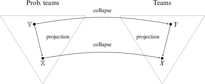

 Open access