2. Mathematical formulation

Consider a two-dimensional gravity-driven incompressible viscous liquid flowing down an inclined plane having an angle $\theta$ with the horizontal in the presence of imposed shear stress $\tau _s$ in the streamwise direction. Suppose that the bounding plane is forced to oscillate sinusoidally with a constant frequency $\omega$ in the streamwise and cross-stream directions, respectively. It is assumed that the density $\rho$ and the dynamic viscosity $\mu$ are constants for a given viscous liquid. Figure 1 shows the schematic diagram of a shear-imposed viscous liquid flowing down a vibrating inclined plane, where the origin of the Cartesian coordinate system is placed at the mid-depth of the unperturbed liquid layer of thickness $2d$, and the axes $x$ and $y$ are chosen along and perpendicular to the plane, respectively. Here $h(x,t)$ represents the deformed liquid surface, and the dashed line in figure 1 represents the undeformed liquid surface. The flow of viscous liquid is described by the usual mass conservation and momentum equations in a reference frame moving with the oscillating inclined plane (Woods & Lin Reference Woods and Lin1995),

(2.1)\begin{gather} \partial_xu + \partial_yv = 0, \end{gather}

(2.2)\begin{gather}\rho (\partial_tu+u\partial_xu +v\partial_yu)=\partial_x\sigma_{xx} +\partial_y\sigma_{xy}+\rho g \sin \theta - \rho A_x\omega^2 \sin \omega t, \end{gather}

(2.3)\begin{gather}\rho (\partial_tv+u\partial_xv + v \partial_yv)=\partial_x\sigma_{yx}+\partial_y\sigma_{yy}-\rho g \cos \theta - \rho A_y\omega^2 \sin \omega t, \end{gather}

where $A_x$ and $A_y$ are, respectively, the forcing amplitudes of streamwise and cross-stream oscillations, $u$ and $v$ are, respectively, the streamwise and cross-stream velocity components of the liquid, and $g$ is the acceleration due to gravity. Here $\sigma _{ij}$ is the stress tensor defined by

(2.4)\begin{equation} \sigma_{ij}={-}p \delta_{ij}+2\mu e_{ij},\quad i,j=1,2, \end{equation}

where $\delta _{ij}$ is the Kronecker delta, $p$ is the pressure and $e_{ij}=1/2(\partial _{i}u_j+\partial _{j}u_i$) is the rate of strain tensor. It should be useful to mention here that additional acceleration terms $A_x\omega ^2 \sin \omega t$ and $A_y\omega ^2 \sin \omega t$ associated with the d’Alembert body force are taken into account in the momentum equations (2.2) and (2.3) due to streamwise and cross-stream oscillations of the inclined plane (Woods & Lin Reference Woods and Lin1995). The above flow configuration is subjected to the following boundary conditions. (i) The velocity components must satisfy no-slip and no-penetration conditions at the inclined plane, $y=-d$,

(2.5a,b)\begin{equation} u=0,\quad v=0. \end{equation}

(ii) The balances of tangential and normal stresses at the deformed liquid surface, $y=h(x,t)$, yield the following dynamic boundary conditions (Smith Reference Smith1982, Reference Smith1990; Wei Reference Wei2005a,Reference Weib; Samanta Reference Samanta2014):

(2.6)\begin{gather} \sigma_{xy}[1-(\partial_xh)^{2}]-(\sigma_{xx}-\sigma_{yy}) \partial_xh=\tau_s[1+(\partial_xh)^{2}]^{1/2}, \end{gather}

(2.7)\begin{gather}p_a+[\sigma_{xx}(\partial_xh)^2 -2 \sigma_{xy} \partial_xh+\sigma_{yy}] [1+(\partial_xh)^2]^{{-}1}=\gamma \partial_{xx}h [1+(\partial_xh)^{2}]^{{-}3/2}, \end{gather}

where $\tau _s$ is the magnitude of imposed shear stress, $p_a$ is the ambient pressure and $\gamma$ is the surface tension. (iii) Finally, the evolution of deformed liquid surface, $y=h(x,t)$, is described by the kinematic boundary condition:

(2.8)\begin{equation} \partial_th+ u \partial_xh=v. \end{equation}

In accordance with the study of Woods & Lin (Reference Woods and Lin1995), the above governing equations are normalised by $d$ as the length scale, $\omega d$ as the velocity scale, $1/\omega$ as the time scale and $\rho (\omega d)^2$ as the pressure scale. Consequently, we can obtain the following non-dimensional numbers: $Re=(\omega d)d/\nu$, the Reynolds number shows the effect of forcing frequency; $Fr=\omega d/\sqrt {gd}$, the Froude number shows the effect of gravity; $We=\gamma /[\rho (\omega d)^2d]$, the Weber number shows the effect of surface tension; and $\tau =\tau _s/(\mu \omega )$, the non-dimensional magnitude of imposed shear stress. Note that the Reynolds number $Re$ compares the square of half-unperturbed liquid layer thickness $d^2$ with the square of Stokes layer thickness $\nu /\omega$. In fact, the current Reynolds number $\omega d^2/\nu$ is equivalent to the square of the Womersley number $Wo$, which is generally relevant for the study of pulsatile flow (Womersley Reference Womersley1955). In particular, the square of the Womersley number $Wo$ compares the viscous time scale $d^2/\nu$ with the frequency time scale $1/\omega$ for a pulsatile flow. It should be useful to mention here that the numerical results will be produced for a wide variety of liquids ranging from water to silicon oil with density $\rho =0.97 \times 10^{3} \ \textrm {Kg}\ \textrm {m}^{-3}$, kinematic viscosity $\nu =10 \times 10^{-4}\ \textrm {m}^2\ \textrm {s}^{-1}$ and surface tension $\gamma =21.2 \times 10^{-3}\ \textrm {N}\ \textrm {m}^{-1}$ (Lin et al. Reference Lin, Chen and Woods1996). Consider a unidirectional parallel flow, the so-called base flow, with an unperturbed viscous liquid layer thickness $y=2d$, which simplifies the governing equations (2.1)–(2.8) into the following non-dimensional forms in a reference frame moving with the oscillating inclined plane:

(2.9)\begin{gather} \partial_tU={-}\partial_xP+\partial_{yy}U/Re+\sin \theta/Fr^2 -a_x \sin t, \end{gather}

(2.10)\begin{gather}\partial_yP+\cos \theta/Fr^2 +a_y \sin t =0, \end{gather}

(2.11)\begin{gather}U=0,\quad \textrm{at}\ y={-}1, \end{gather}

(2.12)\begin{gather}\partial_yU=\tau,\quad P=P_a,\quad \textrm{at}\ y=1, \end{gather}

where $P_a=p_a/[\rho (\omega d)^2]$ is the non-dimensional ambient pressure, and $a_x=A_x/d$ and $a_y=A_y/d$ are, respectively, the non-dimensional forcing amplitudes of streamwise and cross-stream oscillations. The above unsteady base flow equations (2.10)–(2.12) for an unperturbed parallel flow are solved analytically and its exact solution can be expressed as

(2.13)\begin{gather} \hspace{-5pc} U(y,t)=\underbrace{\dfrac{Re \sin \theta}{2 Fr^2}(3+2y-y^{2})+\tau(1+y)}_{{\rm Steady\;part}}\nonumber\\ \hspace{3pc} + \underbrace{a_x\cos t-a_x\mathscr{R}\left[\frac{\cosh\{\beta(1+i)(y-1)\}\,\textrm{e}^{\textrm{i}t}}{\cosh\{2\beta(1+i)\}}\right]}_{{\rm Unsteady\;part}}, \end{gather}

(2.14a,b)\begin{gather} P(y,t)=P_a+\left[\frac{\cos\theta}{Fr^2}+a_y\sin t\right](1-y),\quad V(y,t)=0, \end{gather}

where $\beta =\sqrt {Re/2}$ and $\mathscr {R}[\cdots ]$ represents the real part of that complex function. Obviously, the exact solution of the unperturbed parallel flow depends linearly with the imposed shear stress $\tau$, where both base velocity and base pressure are time-dependent. In particular, the steady part of the base velocity $U(y,t)$ enhances with the increasing value of imposed shear stress $\tau$, but its maximum value no longer exists at the liquid surface on account of the presence of imposed shear stress. Further, it recovers the base flow solution derived by Woods & Lin (Reference Woods and Lin1995) and Lin et al. (Reference Lin, Chen and Woods1996) very well when the imposed shear stress $\tau$ vanishes. Differences in coefficients are the consequence of the definition of Froude number.

Figure 1. Schematic diagram of a shear-imposed viscous liquid flowing down a vibrating inclined plane.

3. Time-dependent Orr–Sommerfeld-type boundary value problem

In order to develop a time-dependent Orr–Sommerfeld-type boundary value problem (OS BVP), we consider an infinitesimal perturbation to the base flow. Accordingly, each flow variable of the disturbed flow can be decomposed as

(3.1)\begin{equation} q(x,y,t)=Q(y,t)+q'(x,y,t), \end{equation}

where $Q(y,t)$ represents the base flow variables and $q'(x,y,t)$ represents the perturbation flow variables. Inserting (3.1) in the governing equations (2.1)–(2.8) and linearising with respect to the base flow solution, one can obtain the following non-dimensional perturbation equations:

(3.2)\begin{gather} \partial_xu'+\partial_yv'=0, \end{gather}

(3.3)\begin{gather}\partial_tu' + U\partial_xu'+v'\partial_yU={-}\partial_xp'+(\partial_{xx}u'+\partial_{yy}u')/Re, \end{gather}

(3.4)\begin{gather}\partial_tv'+U\partial_xv'={-}\partial_yp'+(\partial_{xx}v'+\partial_{yy}v')/Re, \end{gather}

(3.5)\begin{gather}u'=0,\quad v'=0,\quad \textrm{at}\ y={-}1, \end{gather}

(3.6)\begin{gather}(\partial_yu'+\partial_xv'+h'\partial_{yy}U)=0,\quad \textrm{at}\ y=1, \end{gather}

(3.7)\begin{gather}-p'+(\cos \theta /Fr^2 + a_y \sin t)h'+2\partial_yv'/Re-2\partial_{y}U \partial_{x}h'/Re=We\partial_{xx}h', \quad \textrm{at}\ y=1, \end{gather}

(3.8)\begin{gather}\partial_th' + U\partial_xh'=v',\quad \textrm{at}\ y=1. \end{gather}

Now the stream function $\psi '$ is introduced from the perturbation mass conservation equation (3.2) by using the relations $u'=\partial _y\psi '$ and $v'=-\partial _x\psi '$. Substituting the expressions of $u'$ and $v'$ in the perturbation equations (3.2)–(3.8) and eliminating the pressure term from the momentum equations, we seek the solution in the form of a normal mode,

(3.9a,b)\begin{equation} \psi'(x,y,t)=\phi(y,t) \exp(\textrm{i}kx),\quad h'(x,t)=\eta(t)\exp(\textrm{i}kx), \end{equation}

where $k$ is the wavenumber of infinitesimal disturbance, and $\phi$ and $\eta$ are, respectively, the amplitudes of perturbation stream function and surface deformation. Using the normal mode solution (3.9a,b) in the perturbation equations, one can obtain the following time-dependent OS BVP:

(3.10)\begin{gather} \mathscr{L} \partial_t\phi=\mathscr{L}^2\phi/Re-\textrm{i}k(U\mathscr{L}-\mathscr{D}^2U)\phi, \end{gather}

(3.11)\begin{gather}\phi=0,\quad \mathscr{D}\phi=0,\quad \mbox{at}\ y={-}1, \end{gather}

(3.12)\begin{gather}(\mathscr{D}^2+k^2)\phi + \mathscr{D}^2U\eta=0,\quad \textrm{at}\ y=1, \end{gather}

(3.13)\begin{gather} \mathscr{D}\partial_t\phi = (\mathscr{L}-2k^2)\mathscr{D}\phi/Re-(\cos \theta/Fr^2+ a_y \sin t +k^2We -2\textrm{i}k\mathscr{D}U/Re)\textrm{i}k\eta\nonumber\\ \hspace{-7.5pc} -\textrm{i}k(U\mathscr{D}\phi-\mathscr{D}U\phi),\quad \textrm{at}\ y=1, \end{gather}

(3.14)\begin{gather} \partial_t\eta ={-}\textrm{i}k\phi - \textrm{i}kU \eta,\quad \textrm{at}\ y=1,\end{gather}

where $\mathscr {L}=(\mathscr {D}^2-k^2)$ and $\mathscr {D}=\textrm {d}/{\textrm {d} y}$ are differential operators. It should be noted that two new terms arise in the normal stress boundary condition (3.13) owing to the presence of imposed shear stress at the liquid surface. Further, the above time-dependent boundary value problem (3.10)–(3.14) exactly coincides with that derived by Woods & Lin (Reference Woods and Lin1995) when the magnitude of imposed shear stress vanishes, and if the effect of streamwise oscillation of the bounding plane is ignored from the present flow configuration ($a_x=0$).

4. Numerical method

In this section, we shall briefly discuss the numerical method implemented to solve the time-dependent OS BVP (3.10)–(3.14) for disturbances of arbitrary wavenumbers. Actually, a different numerical method from Woods & Lin (Reference Woods and Lin1995) is used to tackle the time-dependent OS BVP. Using the Chebyshev spectral collocation method (Schmid & Henningson Reference Schmid and Henningson2001), the time-dependent OS BVP is first recast into a matrix differential equation with time-periodic coefficients (Or Reference Or1997; Or & Kelly Reference Or and Kelly1998; Samanta Reference Samanta2017, Reference Samanta2019),

(4.1)\begin{equation} \mathbb{B} \partial_t \varPhi= \mathbb{A} \varPhi + (\mathbb{F}_c\cos t+ \mathbb{F}_s\sin t)\varPhi, \end{equation}

where $\varPhi =[\phi _0,\phi _1,\ldots ,\phi _m,\eta ]^\textrm {T}$ is a column matrix, and $\mathbb {A}$, $\mathbb {B}$, $\mathbb {F}_c$ and $\mathbb {F}_s$ are $(m+2) \times (m+2)$ square matrices, $m$ being the number of Chebyshev modes. Next, the matrix equation (4.1) is solved based on Floquet theory (Or Reference Or1997; Samanta Reference Samanta2017, Reference Samanta2020a). Thereby, the time-dependent function $\varPhi (t)$ is expanded in a truncated complex Fourier series from $-K_t$ to $K_t$ as follows:

(4.2)\begin{equation} \varPhi(t)=\sum_{n={-}K_t}^{n=K_t}\varPhi_n\exp[(\textrm{i} n + \delta)t], \end{equation}

where $\varPhi _n$ are constant-coefficient column vectors, $\delta =\delta _r+\textrm {i}\delta _i$ is the complex Floquet exponent, and $n$ and $K_t$ are integers. In fact, $\delta _r$ indicates the temporal growth rate of infinitesimal disturbance. If $\delta _r>0$, the amplitude of infinitesimal disturbance will grow exponentially with time and the corresponding flow will be unstable. Otherwise, the infinitesimal disturbance will decay exponentially with time and the corresponding flow will be stable if $\delta _r<0$. Here we shall focus on both subharmonic ($\delta _i=1/2$) and harmonic ($\delta _i=0$) solutions rather than the harmonic solution merely observed for a liquid flow over a horizontal oscillatory plane (Or Reference Or1997; Samanta Reference Samanta2017, Reference Samanta2019). Substituting (4.2) in the matrix differential equation (4.1) and collecting the coefficient of $\exp [(\textrm {i} n + \delta ) t]$, one can obtain a recurrence relation,

(4.3)\begin{equation} [\mathbb{A}-(\delta +\textrm{i}n)\mathbb{B}]\varPhi_n+\mathbb{F}\varPhi_{n+1}+\mathbb{F}^*\varPhi_{n-1}=0, \end{equation}

where $\mathbb {F}=(\mathbb {F}_c+\textrm {i}\mathbb {F}_s)/2$ and where $\mathbb {F}^*$ is the complex conjugate of $\mathbb {F}$. Indeed, the above recurrence relation (4.3) is a linear system in terms of variables $\varPhi _{n+1}$, $\varPhi _n$ and $\varPhi _{n-1}$, whose coefficients are simply the square matrices. The linear system (4.3) can be turned into a matrix eigenvalue problem (Garih et al. Reference Garih, Strzelecki, Casalis and Estivalezes2013, Reference Garih, Julius, Estivalezes and Casalis2017),

(4.4)\begin{equation} \mathbb{M}\mathbb{X}=\delta \mathbb{N}\mathbb{X}, \end{equation}

where the Floquet exponent $\delta$ is the eigenvalue, $\mathbb {X}=[\varPhi _{-K_t},\varPhi _{-(K_t-1)},\ldots ,\varPhi _{(K_t-1)},\varPhi _{K_t}]^\textrm {T}$ is a column matrix, and $\mathbb {M}$ and $\mathbb {N}$ are, respectively, the block tridiagonal and block diagonal square matrices of the forms

(4.5) \begin{equation} \mathbb{M}=\begin{pmatrix} \vdots & \vdots & \vdots & \vdots & \vdots & \vdots & \vdots \\ \cdots & (\mathbb{A}+2\textrm{i}\mathbb{B}) & \mathbb{F} & 0 & 0 & 0 & \cdots \\ \cdots & \mathbb{F}^{*} & (\mathbb{A}+\textrm{i}\mathbb{B}) & \mathbb{F} & 0 & 0 & \cdots \\ \cdots & 0 & \mathbb{F}^{*} & \mathbb{A} & \mathbb{F} & 0 & \cdots \\ \cdots & 0 & 0 & \mathbb{F}^{*} & (\mathbb{A}-\textrm{i}\mathbb{B}) & \mathbb{F} & \cdots \\ \cdots & 0 & 0 & 0 & \mathbb{F}^{*} & (\mathbb{A}-2\textrm{i}\mathbb{B}) & \cdots \\ \vdots & \vdots & \vdots & \vdots & \vdots & \vdots & \vdots \end{pmatrix}\end{equation}

and

(4.6) \begin{equation} \mathbb{N}=\begin{pmatrix} \vdots & \vdots & \vdots & \vdots & \vdots & \vdots & \vdots \\ \cdots & \mathbb{B} & 0 & 0 & 0 & 0 & \cdots \\ \cdots & 0 & \mathbb{B} & 0 & 0 & 0 & \cdots \\ \cdots & 0 & 0 & \mathbb{B} & 0 & 0 & \cdots \\ \cdots & 0 & 0 & 0 & \mathbb{B} & 0 & \cdots \\ \cdots & 0 & 0 & 0 & 0 & \mathbb{B} & \cdots \\ \vdots & \vdots & \vdots & \vdots & \vdots & \vdots & \vdots\end{pmatrix}. \end{equation}

In the numerical simulation, we shall mainly search for the eigenvalues whose real parts are positive ($\delta _r>0$), because eigenvalues with negative real parts ($\delta _r<0$) will provide stable modes and are not relevant for the instability analysis. Further, the neutral stability curve will be determined numerically by vanishing the real part of the Floquet exponent ($\delta _r=0$) for a given set of flow parameters.

4.1. Spectrum convergence test

A convergence test of the spectrum obtained numerically from the eigenvalue problem (4.4) is accomplished by computing the relative error for twenty least stable eigenvalues with maximum real parts when the number of Chebyshev polynomials varies. Accordingly, the relative error is defined as (Tilton & Cortelezzi Reference Tilton and Cortelezzi2008; Garih et al. Reference Garih, Strzelecki, Casalis and Estivalezes2013; Samanta Reference Samanta2020b)

(4.7)\begin{equation} { \rm{relative\ error}} = \frac{\|\mathscr{R}(\delta_{m+1})-\mathscr{R}(\delta_{m})\|_2}{\|\mathscr{R}(\delta_{m})\|_2}, \end{equation}

where $\mathscr {R}(\delta _{m})$ represents the real parts of eigenvalues, $\|.\|_2$ represents the $L_2$ norm and $m$ is the number of Chebyshev polynomials. Figure 2(a) illustrates the variation of relative error with the number of Chebyshev polynomials when the number of Fourier modes is fixed ($K_t=15$). The results are produced for several values of the Reynolds number when $\tau =0.5$ and $a_x=0$ are fixed. Apparently, it seems that at least twenty Chebyshev modes ($m \ge 20$) and fifteen Fourier modes ($K_t=15$) are sufficient to have accurate numerical results for the Reynolds number $Re=5$, because the associated relative error saturates approximately to order $O(10^{-9})$. However, we need at least forty Chebyshev modes ($m \ge 40$) and fifteen Fourier modes ($K_t=15$) to achieve accurate numerical results when Reynolds number $Re=100$, because the associated relative error saturates approximately to order $O(10^{-10})$. Obviously, the above results suggest that we require more Chebyshev polynomials for accurate numerical results at higher Reynolds number. On the other hand, figure 2(b) illustrates the spectrum obtained numerically from the eigenvalue problem (4.4) when the imposed shear stress alters from $\tau =0$ to $\tau =0.6$ but $a_x=0$ is fixed. The eigenvalues show almost a vertical straight line pattern at $\tau =0$, specified by circular points. As soon as $\tau$ increases, the real parts of eigenvalues move slightly right while the imaginary parts move slightly down, specified by dot points (see the inset of figure 2b). Therefore, one can envisage that the external imposed shear stress has a destabilising effect on the parametric instability or Faraday instability for a vertical falling film where the bounding plane oscillates only in the cross-stream direction. It should be fruitful to mention here that spurious eigenvalues may appear in the numerical solution because of the homogeneous boundary conditions (3.11) used in the rows of matrix $\mathbb {A}$. However, these spurious eigenvalues are mapped to the arbitrary irrelevant stable modes by carefully selecting the complex multiple for the corresponding rows of matrix $\mathbb {B}$ (Schmid & Henningson Reference Schmid and Henningson2001). In this way, one can avoid spurious eigenvalues from the matrix eigenvalue problem (4.4).

Figure 2. (a) Convergence of the spectrum with the number of Chebyshev polynomials when $\tau =0.5$. Star, dot and circle points are results for $Re=100$, $Re=30$ and $Re=5$, respectively. (b) Variation of the eigenvalue spectrum obtained from (4.4) when $\tau \in [0, 0.6]$. The other flow parameters are $a_x=0$, $a_y=1$, $k=1$, $We=0.016$, $Fr^2=100$, $Re=5$ and $\theta =90^{\circ }$. Inset figure shows the variation of eigenvalues with positive real parts.

4.2. Validation of the numerical method

Before producing the current results, the above numerical code is validated with the available results for a viscous liquid flowing down a vibrating inclined plane without imposed shear stress (Woods & Lin Reference Woods and Lin1995). Consequently, the effect of imposed shear stress is removed from the current flow configuration by setting $\tau =0$. Further, it is assumed that the plane oscillates solely in the cross-stream direction, i.e. $a_x=0$. Following Woods & Lin (Reference Woods and Lin1995), we select $We=0.016$, $Fr^2=100$, $Re=5$ and $\theta =90^{\circ }$ in the numerical experiment. Figure 3(a) displays the neutral curve in the (wavenumber, forcing amplitude)-plane for the given set of parameter values. The neutral curve exhibits three distinct regimes pertaining to the gravitational, subharmonic and harmonic instabilities as demonstrated by Woods & Lin (Reference Woods and Lin1995), where the gravitational instability occurs in the long-wave regime, but the subharmonic and harmonic instabilities occur in the finite wavelength regime. Further, it should be noted that the subharmonic and harmonic instability zones have tongue-like shapes (Kumar & Tuckerman Reference Kumar and Tuckerman1994; Kumar Reference Kumar1996) with wide unstable ranges of wavenumber, where the first subharmonic tongue is lower than the first harmonic tongue. This phenomenon implies that the resonated wave will evolve initially in the finite wavelength regime through the subharmonic instability. In particular, the appearance of gravitational instability is responsible for the streamwise component of gravitational force while the appearances of subharmonic and harmonic instabilities are responsible for the cross-stream oscillation of the bounding plane. Therefore, one can excite subharmonic and harmonic resonances by applying a cross-stream oscillation to the bounding plane with a given forcing amplitude. On the other hand, figure 3(b) displays the variation of temporal growth rate for the gravitational instability when the forcing amplitude $a_y$ of cross-stream oscillation varies. It is evident that the gravitational instability raises irrespective of the zero value of forcing amplitude of the cross-stream oscillation. Hence, the external oscillatory d’Alembert body force attributed normal to the bounding plane is not required to generate the gravitational instability. The streamwise gravitational force is sufficient to have gravitational instability. On the contrary, an external oscillatory forcing is essential for the subharmonic and harmonic instabilities (see figure 3a). As discussed by Woods & Lin (Reference Woods and Lin1995), the temporal growth rate for the gravitational instability attenuates gradually with the increasing value of forcing amplitude. However, it cannot be fully eliminated from the temporal growth profile by setting a larger value to the forcing amplitude $a_y$. Further, the reduction of maximum temporal growth rate with the increasing value of forcing amplitude $a_y$ can be found in table 1, which agrees very well with the available results of Garih et al. (Reference Garih, Strzelecki, Casalis and Estivalezes2013) and Jaouahiry & Aniss (Reference Jaouahiry and Aniss2020) when the imposed shear stress is neglected ($\tau =0$), and there is no streamwise oscillation of the bounding plane ($a_x=0$). Therefore, one can cause the gravitational instability to deteriorate, or one can delay the transition of gravitational instability to turbulence, by applying a perpendicular oscillation to the bounding plane. In addition, the temporal growth profile and the neutral curve capture the results of Woods & Lin (Reference Woods and Lin1995) very well in the absence of imposed shear stress, and if the streamwise oscillation of the bounding plane is ignored ($a_x=0$).

Figure 3. (a) Variation of neutral curve in the (wavenumber, forcing amplitude)-plane. (b) Variation of temporal growth rate $\delta _r$ for the gravitational instability when the forcing amplitude of cross-stream oscillation $a_y$ varies. Solid, dashed, dotted and dash-dotted lines stand for $a_y=0$, $a_y=0.1$, $a_y=0.2$ and $a_y=2$, respectively. The other flow parameters are $a_x=0$, $\tau =0$, $We=0.016$, $Fr^2=100$, $Re=5$ and $\theta =90^{\circ }$. Circular points are results of Woods & Lin (Reference Woods and Lin1995). Here ‘SH’ and ‘H’ represent the subharmonic and harmonic instability zones, respectively.

Table 1. Comparison of maximum temporal growth rate for the gravitational instability when the forcing amplitude of cross-stream oscillation $a_y$ alters. The other flow parameters are $a_x=0$, $We=0.016$, $Fr^2=100$, $Re=5$, $\theta =90^{\circ }$ and $\tau =0$.

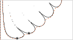
In order to verify with the result of streamwise oscillatory liquid flow falling down a vertical plane without an imposed shear stress (Lin et al. Reference Lin, Chen and Woods1996), we set $\tau =0$, $We=0.016$, $Fr^2=10\,000$ and $\theta =90^{\circ }$ in the numerical experiment. In this case, it is assumed that the plane oscillates solely in the streamwise direction, i.e. $a_y=0$. The ensuing result is displayed in figure 4 for several values of forcing amplitude $a_x$ of the streamwise oscillation. It is found that there exists only one unstable zone associated with the gravitational instability in the (Reynolds number, wavenumber)-plane when $a_x=0$. The result is specified by a dash-dotted line in figure 4. As soon as the streamwise oscillatory forcing is introduced, i.e. if the forcing amplitude of streamwise oscillation is non-zero, one unstable zone is divided into three separate unstable zones. In fact, the first two unstable zones, I and II, are created due to the streamwise oscillation of the bounding plane. Further, the first two unstable zones, I and II, enhance, while the third unstable zone, III, reduces with the increasing value of forcing amplitude $a_x$ of the streamwise oscillation. The interesting result is that the primary instability is driven by the gravitational instability at the outset when there is no external forcing. As soon as the external streamwise oscillatory forcing is applied to the bounding plane, the primary instability is no longer driven by the gravitational instability at the outset. Instead, the resonated instability dominates the primary instability when the Reynolds number is small. Further, there exist some stable ranges of Reynolds number, or equivalently, some stable bandwidths of forcing frequency where the unstable vertical falling liquid film becomes stable due to streamwise oscillation of the bounding plane. Indeed, the stable frequency bandwidths condense, and the primary instability is gradually triggered by the gravitational instability with the decreasing value of forcing amplitude as expected. Therefore, one can obtain some stable ranges of Reynolds number despite the vertical falling liquid film if the plane is forced to oscillate in the streamwise direction. Moreover, the present result captures the result of Lin et al. (Reference Lin, Chen and Woods1996) very well in an appropriate limit. The above facts fully confirm the accuracy of the current numerical code.

Figure 4. Neutral curve in the (Reynolds number, wavenumber)-plane for different values of forcing amplitude $a_x$ of the streamwise oscillation. Solid, dashed, dotted and dash-dotted lines stand for $a_x=6$, $a_x=5$, $a_x=4$ and $a_x=0$, respectively. The other flow parameters are $a_y=0$, $\tau =0$, $We=0.016$, $Fr^2=10\,000$ and $\theta =90^{\circ }$. Here ‘$S$’ and ‘$U$’ represent the stable and unstable zones, respectively. Inset figure shows the neutral curve for the gravitational instability. Solid points are results of Lin et al. (Reference Lin, Chen and Woods1996).

5. Effect of imposed shear stress for a cross-stream oscillatory flow

This section deals with the oscillation normal to the plane only, i.e. there is no streamwise oscillation of the bounding plane ($a_x=0$). In order to investigate the effect of imposed shear stress $\tau$ on the parametric instability or Faraday instability for an oscillatory liquid flowing down a vertical plane, we set $We=0.016$, $Fr^2=100$, $Re=5$ and $\theta =90^{\circ }$ in the numerical experiment. Basically, the numerical experiment is carried out for a comparatively thicker layer of liquid flow with small surface tension when the forcing frequency of cross-stream oscillation is low. Figure 5 depicts the neutral curve in the (wavenumber, forcing amplitude)-plane when the imposed shear stress alters. The neutral curve shows the existence of gravitational, subharmonic and harmonic instabilities for the given set of parameter values. Hence, one can resonate subharmonic and harmonic instabilities in different unstable ranges of wavenumber by varying the forcing amplitude of cross-stream oscillation at $\tau =0$. In particular, the subharmonic and harmonic instability zones exhibit tongue-like shapes with wide unstable ranges of wavenumber. Further, subharmonic and harmonic instabilities will be excited once the forcing amplitude of cross-stream oscillation $a_y$ exceeds the respective critical amplitudes for the subharmonic and harmonic instabilities, which are indicated by star points in figure 5. For instance, the critical amplitude for the first subharmonic instability appears at $a_y=0.79$ when the wavenumber $k=1.18$. On the other hand, the critical amplitude for the first harmonic instability appears at $a_y=3.44$ when the wavenumber $k=1.87$. More specifically, the subharmonic instability will occur first because the critical amplitude for the appearance of first subharmonic wave is less than that for the appearance of the first harmonic wave. Apparently, it seems that there exist stable ranges of wavenumber between gravitational and subharmonic instabilities as well as between subharmonic and harmonic instabilities, where the flow system cannot be susceptible to instability by the oscillating plane in the normal direction with a given forcing amplitude. In other words, the gravitational instability switches to subharmonic instability as well as the subharmonic instability switching to harmonic instability in a discontinuous manner for a given forcing amplitude when the wavenumber increases. As soon as the imposed shear stress is incorporated in the numerical experiment, the stable range which emerged in the long-wave regime between gravitational and subharmonic instabilities becomes narrower, and the stable range which emerged in the finite wavenumber regime between subharmonic and harmonic instabilities completely disappears at $\tau =0.6$. If the imposed shear stress is further increased to $\tau =0.9$, the long-wave unstable range of wavenumber responsible for the gravitational instability attenuates, but does not fully disappear from the (wavenumber, forcing amplitude)-plane because flow occurs on a vertical oscillating plane ($\theta =90^{\circ }$). It seems that the transition from gravitational instability to subharmonic instability occurs rapidly in a discontinuous manner, while the transition from subharmonic instability to harmonic instability occurs in a continuous manner with the increasing value of wavenumber for an oscillatory shear-imposed flow with a given forcing amplitude. In addition, the critical amplitudes for the subharmonic and harmonic instabilities decrease with the increasing value of $\tau$. Therefore, one can generate subharmonic and harmonic instabilities, comparatively, at lower forcing amplitudes for a cross-stream oscillatory shear-imposed flow. In order to figure out the temporal growth rates for the parametric resonances, the numerical test is repeated again for different values of the forcing amplitude $a_y$. The results can be found in figure 6. If the plane is forced to oscillate normally with amplitude $a_y=1$, the temporal growth profile reveals two humps, where the first hump associated with the gravitational instability appears in the long-wave regime, while the second hump associated with the subharmonic instability appears in the finite wavelength regime. However, the maximum temporal growth rate for the subharmonic instability is always much larger than that for the gravitational instability. It should be noted that the temporal growth rates for both gravitational and subharmonic instabilities enhance with the increasing value of imposed shear stress when $a_y=1$. Therefore, the gravitational and subharmonic instabilities intensify in the presence of imposed shear stress at low forcing amplitude for a low-Reynolds-number flow. In this case, the harmonic instability cannot be excited because the forcing amplitude $a_y$ is not sufficient to resonate harmonic wave (see figure 6a). Obviously, there exists a stable range of wavenumber between gravitational and subharmonic instabilities, where the temporal growth rate is completely negative and this stable range gradually becomes narrower with the increasing value of $\tau$. This fact is fully consistent with the result reported in figure 5. As soon as the forcing amplitude of cross-stream oscillation is increased to $a_y=4$, the temporal growth profile reveals three humps rather than two. A new hump associated with the harmonic instability appears along with the gravitational and subharmonic instabilities, where the gravitational instability prevails in the long-wave regime followed by subharmonic and harmonic instabilities in the finite wavelength regime (see figure 6b). The maximum temporal growth rate for the subharmonic instability is larger than those for the gravitational and harmonic instabilities. The interesting fact is that the temporal growth rates for the gravitational and harmonic instabilities amplify, but the temporal growth rate for the subharmonic instability depletes with the increasing value of imposed shear stress as opposed to the result when $a_y=1$ (see figure 6a). Therefore, the gravitational and harmonic instabilities become stronger, but the subharmonic instability becomes weaker in the presence of imposed shear stress at high forcing amplitude for a low-Reynolds-number flow. In this case, the maximum temporal growth rate for the subharmonic instability is no longer larger than that for the harmonic instability. Instead, an opposite phenomenon happens, i.e. the maximum temporal growth rate for the harmonic instability is larger than that for the subharmonic instability at $\tau =0.8$. Further, there exist stable ranges of wavenumber between gravitational and subharmonic instabilities as well as between subharmonic and harmonic instabilities when $a_y=4$ and $\tau =0$. However, the stable range emerged in the long-wave regime between gravitational and subharmonic instabilities becomes narrower as long as $\tau$ increases. On the other hand, the stable range emerged in the finite wavenumber regime between subharmonic and harmonic instabilities no longer exists with the increasing value of $\tau$. Hence, one can conclude that there eventuates a continuous switching from subharmonic instability to harmonic instability in the finite wavenumber regime for a shear-imposed low Reynolds number flow if a normal oscillation is attributed to the bounding plane with higher forcing amplitude. In this case, the subharmonic resonance can be made weaker by applying a constant shear stress at the liquid surface in the streamwise direction.

Figure 5. Neutral curve in the (wavenumber, forcing amplitude)-plane for different values of $\tau$. Solid, dashed and dotted lines stand for $\tau =0$, $\tau =0.6$ and $\tau =0.9$, respectively. The other flow parameters are $a_x=0$, $We=0.016$, $Fr^2=100$, $Re=5$ and $\theta =90^{\circ }$. Here ‘SH’ and ‘H’ represent the subharmonic and harmonic instability zones, respectively. Star points represent the critical amplitudes for the first subharmonic and first harmonic instabilities at $\tau =0$.

Figure 6. Variation of temporal growth rate with the wavenumber for different values of $\tau$. Solid, dashed, dotted and dash-dotted lines stand for $\tau =0$, $\tau =0.3$, $\tau =0.6$ and $\tau =0.8$, respectively. Flow parameters are (a) $a_y=1$ and (b) $a_y=4$. The other flow parameters are $a_x=0$, $We=0.016$, $Fr^2=100$, $Re=5$ and $\theta =90^{\circ }$. Inset figures show the temporal growth rate for the gravitational instability.

Next, we perform the numerical experiment for $Re=30$ when other flow parameters remain the same as supplied in figure 5. In this case, we are actually increasing the forcing frequency of cross-stream oscillation. The associated result is illustrated in figure 7. The neutral curve pertaining to the resonated waves exhibits tongue-like shapes as depicted in figure 5. The unstable range of wavenumber for the gravitational instability enhances with the increasing value of Reynolds number when $\tau =0$. Further, the critical amplitudes for the first subharmonic and first harmonic instabilities reduce significantly in comparison with the result when $Re=5$ and $\tau =0$. In fact, one can create resonated waves, comparatively, at lower forcing amplitudes for a moderate Reynolds number cross-stream oscillatory flow. If the effect of imposed shear stress is incorporated in the numerical experiment, the stable range between gravitational and subharmonic instabilities reduces. Therefore, the presence of imposed shear stress makes the transition faster from gravitational instability to subharmonic instability. Furthermore, with the increasing value of forcing frequency of cross-stream oscillation, or equivalently, with the increasing value of Reynolds number, the temporal growth rate shows an opposite scenario of figure 6(a) with varying $\tau$. The results are demonstrated in figure 8. Obviously, there exist three humps instead of two in the temporal growth profile for a non-zero value of imposed shear stress (see figure 8a). The temporal growth rates for the gravitational and subharmonic instabilities attenuate rather than enhance with the increasing value of imposed shear stress at low forcing amplitude ($a_y=1$). Therefore, one can make weaker the maximum values of temporal growth rates for the subharmonic resonance and gravitational instability by incorporating external shear stress at the liquid surface for a shear-imposed flow with moderate Reynolds number. Further, the harmonic resonance also emerges at low forcing amplitude in a separate unstable range of wavenumber along with the subharmonic resonance for a non-zero value of imposed shear stress $\tau$ and intensifies with the increasing value of imposed shear stress. As soon as the forcing amplitude of cross-stream oscillation is shifted to a comparatively higher value ($a_y=3$), a new hump associated with the subharmonic instability is introduced in the temporal growth profile together with the remaining three humps (see figure 8b). However, the first three humps become weaker while the fourth hump becomes stronger with the increasing value of imposed shear stress.

Figure 7. Neutral curve in the (wavenumber, forcing amplitude)-plane for different values of $\tau$. Solid and dashed lines stand for $\tau =0$ and $\tau =0.3$, respectively. The other flow parameters are $a_x=0$, $We=0.016$, $Fr^2=100$, $Re=30$ and $\theta =90^{\circ }$. Here ‘SH’ and ‘H’ represent the subharmonic and harmonic instability zones, respectively. Star points represent the critical amplitudes for the first subharmonic and first harmonic instabilities at $\tau =0$.

Figure 8. Variation of temporal growth rate with the wavenumber for different values of $\tau$. Solid, dashed, dotted and dash-dotted lines stand for $\tau =0$, $\tau =0.3$, $\tau =0.6$ and $\tau =0.8$, respectively. Flow parameters are (a) $a_y=1$ and (b) $a_y=3$. The other flow parameters are $a_x=0$, $We=0.016$, $Fr^2=100$, $Re=30$ and $\theta =90^{\circ }$. Inset figures show the temporal growth rate for the gravitational instability.

If the numerical experiment is performed for a comparatively thinner layer of oscillatory liquid flow, or equivalently, if the Froude number is decreased and set to $Fr^2=10$, only gravitational and subharmonic instabilities excite in distinct unstable ranges of wavenumber at low forcing amplitude ($a_y=1$). The result is displayed in figure 9(a). It is observed that both gravitational and subharmonic instabilities weaken with the increasing value of imposed shear stress. However, if the forcing amplitude is increased to a comparatively higher value as before ($a_y=3$), the harmonic resonance again rises along with the subharmonic resonance in the finite wavenumber regime (see figure 9b). The harmonic resonance amplifies but the subharmonic resonance attenuates in the presence of imposed shear stress. In this case, the impacts of imposed shear stress on the subharmonic and harmonic resonances are more discernible than the previous cases. Therefore, one can predict that the subharmonic resonance can also be made weaker for a thinner layer of shear-imposed cross-stream oscillatory flow.

Figure 9. Variation of temporal growth rate with the wavenumber for different values of $\tau$. Solid, dashed and dotted lines stand for $\tau =0$, $\tau =0.3$ and $\tau =0.6$, respectively. Flow parameters are (a) $a_y=1$ and (b) $a_y=3$. The other flow parameters are $a_x=0$, $We=0.016$, $Fr^2=10$, $Re=10$ and $\theta =90^{\circ }$. Inset figure shows the temporal growth rate for the gravitational instability.

In order to explore the Faraday instability for a comparatively thicker layer of liquid flow with high surface tension down a slightly inclined plane, we set $We=0.16$, $Fr^2=100$, $Re=10$ and $\theta =1^{\circ }$ in the numerical experiment. Figure 10 illustrates the neutral curve in the (wavenumber, forcing amplitude)-plane when the imposed shear stress alters. It should be noted that the neutral curve exhibits tongue-like shapes followed by subharmonic and harmonic tongues. In particular, the subharmonic and harmonic instabilities occur alternately in these tongue-like unstable zones. However, the unstable ranges of wavenumber for the subharmonic and harmonic tongues squeeze significantly in comparison with the result reported in figure 5 where the Weber number is small ($We=0.016$) and the plane is vertical ($\theta =90^{\circ }$). The interesting result is that the regime of gravitational instability is no longer manifested in the neutral diagram because the associated Reynolds number lies in the stable zone. As soon as the imposed shear stress is incorporated in the numerical experiment, the stable ranges which emerged in the finite wavenumber regime between subharmonic and harmonic tongues completely disappear at $\tau =0.6$. Further, the critical amplitudes for the subharmonic and harmonic tongues decrease with the increasing value of imposed shear stress. But the critical amplitude for the first subharmonic tongue always remains lower than that for the first harmonic tongue. Hence, one can excite subharmonic and harmonic resonances at lower forcing amplitudes for a shear-imposed thinner layer of liquid with high surface tension flowing down a slightly inclined plane. Figure 11 displays the associated temporal growth rates for the Faraday waves when the imposed shear stress changes. It should be noted that there exists a single hump associated with the subharmonic instability at low forcing amplitude ($a_y=1$), which attenuates with the increasing value of $\tau$ (see figure 11a). As soon as the forcing amplitude of cross-stream oscillation is shifted to a comparatively higher value ($a_y=3$), a new hump pertaining to the harmonic instability is introduced in the temporal growth profile along with the remaining hump (see figure 11b). Obviously, the new hump intensifies with the increasing value of $\tau$. Hence, the harmonic resonance can be made stronger by including an imposed shear stress at the liquid surface in the streamwise direction (see figure 11b). Further, there does not exist an additional unstable hump related to the gravitational instability in the temporal growth profile. This fact is fully in favour of the result reported in figure 10. If the forcing frequency, or equivalently, if the Reynolds number is further increased and fixed at $Re=80$ in the numerical experiment, the subharmonic and harmonic tongues compress significantly in comparison with the result shown in figure 10, and consequently, more subharmonic and harmonic tongues appear alternately in distinct unstable ranges of wavenumber (see figure 12). Furthermore, the critical amplitudes for the generation of subharmonic and harmonic resonances significantly decrease with the increasing value of Reynolds number. The gravitational instability disappears from the neutral diagram because the Reynolds number still does not exceed the critical value for the existence of gravitational instability. As soon as the imposed shear stress is included in the numerical experiment, the gravitational instability emerges along with the subharmonic and harmonic resonances in the neutral diagram at $\tau =0.6$ (see figure 12). Basically, the critical Reynolds number for the gravitational instability reduces with the increasing value of imposed shear stress (Smith Reference Smith1990; Samanta Reference Samanta2014) and makes it lower than the given Reynolds number $Re=80$. This fact yields an unstable region for the gravitational instability in the neutral diagram at $\tau =0.6$. Figure 13(a) exhibits the associated temporal growth rate for the resonated wave. It is observed that there exists only one hump in the finite wavenumber regime pertaining to the subharmonic instability at $a_y=0.3$ when $\tau =0$, which attenuates in the presence of imposed shear stress. There do not exist additional humps pertaining to the gravitational and harmonic instabilities at $\tau =0$. However, the gravitational instability arises in the presence of imposed shear stress, which intensifies as long as the imposed shear stress increases. If the forcing amplitude of cross-stream oscillation is shifted to a slightly higher value ($a_y=1$), an additional hump associated with the harmonic instability emerges in the finite wavenumber regime along with the subharmonic instability (see figure 13b). In this case, the harmonic resonance occurs at low forcing amplitude ($a_y=1$) rather than at high forcing amplitude ($a_y=3$), shown in figure 11(b). This result is fully consistent with the result reported in figure 12. Further, both subharmonic and harmonic resonances become weaker in the presence of imposed shear stress. Hence, one can resonate subharmonic and harmonic waves, comparatively, at lower forcing amplitudes for an oscillatory flow with moderate Reynolds number, and the resonated waves can be made weaker by imposing an external shear stress at the liquid surface in the streamwise direction.

Figure 10. Neutral curve in the (wavenumber, forcing amplitude)-plane for different values of $\tau$. Solid and dashed lines stand for $\tau =0$ and $\tau =0.6$, respectively. The other flow parameters are $a_x=0$, $We=0.16$, $Fr^2=100$, $Re=10$ and $\theta =1^{\circ }$. Here ‘SH’ and ‘H’ represent the subharmonic and harmonic instability zones. Star points represent the critical amplitudes for the first subharmonic and first harmonic instabilities at $\tau =0$.

Figure 11. Variation of temporal growth rate with the wavenumber for different values of $\tau$. Solid, dashed and dotted lines stand for $\tau =0$, $\tau =0.3$ and $\tau =0.6$, respectively. Flow parameters are (a) $a_y=1$ and (b) $a_y=3$. The other flow parameters are $a_x=0$, $We=0.16$, $Fr^2=100$, $Re=10$ and $\theta =1^{\circ }$.

Figure 12. Neutral curve in the (wavenumber, forcing amplitude)-plane for different values of $\tau$. Solid and dashed lines stand for $\tau =0$ and $\tau =0.6$, respectively. The other flow parameters are $a_x=0$, $We=0.16$, $Fr^2=100$, $Re=80$ and $\theta =1^{\circ }$. Here ‘SH’ and ‘H’ represent the subharmonic and harmonic instability zones. Star points represent the critical amplitudes for the first subharmonic and first harmonic instabilities at $\tau =0$.

Figure 13. Variation of temporal growth rate with the wavenumber for different values of $\tau$. Solid, dashed and dotted lines stand for $\tau =0$, $\tau =0.3$ and $\tau =0.6$, respectively. Flow parameters are (a) $a_y=0.3$ and (b) $a_y=1$. The other flow parameters are $a_x=0$, $We=0.16$, $Fr^2=100$, $Re=80$ and $\theta =1^{\circ }$.

In order to perform the numerical experiment for a high-Reynolds-number thin layer of liquid with high surface tension flowing down a slightly inclined plane, we set $We=5$, $Fr^2=1$, $Re=293$ and $\theta =1^{\circ }$ (Woods & Lin Reference Woods and Lin1995). The ensuing results are demonstrated in figure 14. Note that there exist two humps in the temporal growth profile pertaining to the gravitational and shear instabilities when there is no external oscillatory forcing (see figure 14a). Obviously, the gravitational instability occurs in the long-wave regime while the shear instability occurs in the finite wavenumber regime. Therefore, a new instability, the so-called shear instability, emerges in the finite wavenumber regime when the Reynolds number is large and the inclination angle is sufficiently small. In fact, in this case, the given Reynolds number exceeds the critical Reynolds number for the appearance of shear instability. Note that both gravitational and shear instabilities amplify with the increasing value of imposed shear stress. Further, the subharmonic and harmonic resonances disappear from the temporal growth profile because the forcing amplitude of cross-stream oscillation vanishes ($a_y=0$). As soon as the forcing amplitude is turned on ($a_y=1$) in the numerical experiment, both subharmonic and harmonic resonances appear in the temporal growth profile along with the gravitational and shear instabilities (see figure 14b). It should be noted that both gravitational and shear instabilities become weaker in the presence of external oscillatory cross-stream forcing. However, they become stronger in the presence of imposed shear stress. On the other hand, the subharmonic and harmonic resonances attenuate with the increasing value of imposed shear stress.

Figure 14. Variation of temporal growth rate with the wavenumber for different values of $\tau$. Solid, dashed and dotted lines stand for $\tau =0$, $\tau =0.3$ and $\tau =0.6$, respectively. Flow parameters are (a) $a_y=0$ and (b) $a_y=1$. The other flow parameters are $a_x=0$, $We=5$, $Fr^2=1$, $Re=293$ and $\theta =1^{\circ }$.

6. Effect of imposed shear stress for a streamwise oscillatory flow

In this section, we shall focus solely on the streamwise oscillation of the bounding plane, i.e. there is no cross-stream oscillation of the bounding plane ($a_y=0$). In order to investigate the effect of imposed shear stress $\tau$ on the parametric instability for a streamwise oscillatory liquid flowing down a vertical plane, we set $a_x=6$, $We=0.016$, $Fr^2=10\,000$ and $\theta =90^{\circ }$ in the numerical experiment (Lin et al. Reference Lin, Chen and Woods1996). Basically, the numerical experiment is carried out for a comparatively thicker layer of liquid flow with small surface tension. Figure 15 displays the neutral curve in the (Reynolds number, wavenumber)-plane when the imposed shear stress alters. The neutral curve exhibits three distinct unstable regions specified by I, II and III for the given set of parameter values. In particular, the unstable regions I and II are developed owing to the streamwise oscillation of the plane, while the third unstable zone, III, is responsible for the gravitational instability. Obviously, the imposed shear stress does not have significant impact on the first resonated unstable zone, I, but the second resonated unstable zone, II, significantly reduces with the increasing value of imposed shear stress. On the other hand, the third unstable zone, III, enhances in the presence of imposed shear stress. Further, there exist stable ranges of Reynolds number, or equivalently, there exist stable ranges of frequency bandwidths where the streamwise oscillatory flow is completely damped to infinitesimal disturbances even though the liquid flow occurs on a vertical plane. It is evident that the stable range of Reynolds number between the resonated unstable zone, II, and the third unstable zone, III, decreases, and ultimately, vanishes from the neutral diagram with the increasing value of imposed shear stress. In other words, the resonated unstable zone, II, and the third unstable zone, III, merge with each other with the increasing value of imposed shear stress. As a consequence, the neutral curve converts into two distinct unstable zones separated by a stable range of Reynolds number at $\tau =0.1$. Further, one can speculate that there occurs a continuous transition from the resonated instability to gravitational instability at higher values of the imposed shear stress. Figure 16 reveals the associated temporal growth rates for the second resonated unstable zone, II, and the third unstable zone, III, when the imposed shear stress varies. It should be noted that the temporal growth rate for the resonated unstable zone, II, attenuates in the presence of imposed shear stress when $Re=12$ (see figure 16a). By contrast, the maximum temporal growth rate for the third unstable zone, III, enhances as soon as the imposed shear stress increases when $Re=30$ (see figure 16b). This fact is fully consistent with the result reported in figure 15. From the above result, one can conclude that the unstable domain of the resonated wave for a streamwise oscillatory flow can be reduced by imposing an external shear stress at the liquid surface in the streamwise direction.

Figure 15. Neutral curve in the (Reynolds number, wavenumber)-plane for different values of $\tau$. Solid, dashed, dotted and dash-dotted lines stand for $\tau =0$, $\tau =0.005$, $\tau =0.05$ and $\tau =0.1$, respectively. The other flow parameters are $a_x=6$, $a_y=0$, $We=0.016$, $Fr^2=10\,000$ and $\theta =90^{\circ }$. Here ‘S’ and ‘U’ represent the stable and unstable zones, respectively.

Figure 16. Variation of temporal growth rate with the wavenumber for different values of $\tau$. Solid, dashed and dotted lines stand for $\tau =0$, $\tau =0.05$ and $\tau =0.1$, respectively. Reynolds numbers are (a) $Re=12$ and (b) $Re=30$. The other flow parameters are $a_x=6$, $a_y=0$, $We=0.016$, $Fr^2=10\,000$ and $\theta =90^{\circ }$.

If the surface tension, or equivalently, the Weber number is reduced and set to $We=0.008$, the numerical result exhibits a similar scenario as shown in figure 15. The neutral curve reveals three unstable regions, I, II and III, separated by the stable ranges of Reynolds number when $\tau =0$ (see figure 17). However, the second resonated unstable zone, II, significantly enhances in comparison with the result reported in figure 15 with the decreasing value of surface tension. As soon as the imposed shear stress is incorporated in the numerical experiment, the first resonated unstable zone, I, does not change considerably as before. But the second resonated unstable zone, II, reduces considerably with the increasing value of imposed shear stress. On the other hand, the third unstable zone, III, enhances, and finally, coalesces with the resonated unstable zone II at higher values of the imposed shear stress. The associated temporal growth rates for the second resonated unstable zone, II, and the third unstable zone, III, are illustrated in figure 18 with the variation of imposed shear stress. Obviously, the temporal growth rate for the resonated unstable zone II becomes weaker in the presence of imposed shear stress when $Re=12$ (see figure 18a). However, the maximum temporal growth rate for the third unstable zone, III, becomes stronger as soon as the imposed shear stress increases when $Re=30$ (see figure 18b). This fact is fully consistent with the result reported in figure 17.

Figure 17. Neutral curve in the (Reynolds number, wavenumber)-plane for different values of $\tau$. Solid, dashed and dotted lines stand for $\tau =0$, $\tau =0.1$ and $\tau =0.2$, respectively. The other flow parameters are $a_x=6$, $a_y=0$, $We=0.008$, $Fr^2=10\,000$ and $\theta =90^{\circ }$. Here ‘S’ and ‘U’ represent the stable and unstable zones, respectively.

Figure 18. Variation of temporal growth rate with the wavenumber for different values of $\tau$. Solid, dashed and dotted lines stand for $\tau =0$, $\tau =0.1$ and $\tau =0.2$, respectively. Reynolds numbers are (a) $Re=12$ and (b) $Re=30$. The other flow parameters are $a_x=6$, $a_y=0$, $We=0.008$, $Fr^2=10\,000$ and $\theta =90^{\circ }$.

In order to analyse the parametric instability for a comparatively thinner layer of oscillatory liquid flow, we set $a_x=6$, $We=0.016$, $Fr^2=100$ and $\theta =90^{\circ }$ in the numerical experiment. In this case, two unstable zones separated by a stable range of Reynolds number are observed in the neutral diagram. The result can be found in figure 19. Apparently, it seems that the first unstable zone, I, develops due to the streamwise oscillation of the bounding plane while the second unstable zone, II, is responsible for the gravitational instability. Further, the first resonated unstable zone, I, does not change significantly but the second unstable zone, II, reduces significantly with the increasing value of imposed shear stress. In addition, the critical Reynolds number for the creation of second unstable zone, II, decreases as long as the imposed shear stress increases, and finally, merges with the resonated unstable zone I at $\tau =0.7$. This fact ensures that the gravitational instability will evolve at a lower Reynolds number in the presence of imposed shear stress for a streamwise oscillatory flow. Further, there occurs a continuous switching from the resonated instability to gravitational instability at higher values of the imposed shear stress.

Figure 19. Neutral curve in the (Reynolds number, wavenumber)-plane for different values of $\tau$. Solid, dashed, dotted and dash-dotted lines stand for $\tau =0$, $\tau =0.1$, $\tau =0.2$ and $\tau =0.7$, respectively. The other flow parameters are $a_x=6$, $a_y=0$, $We=0.016$, $Fr^2=100$ and $\theta =90^{\circ }$. Here ‘S’ and ‘U’ represent the stable and unstable zones, respectively.

Now the numerical experiment is performed for a high-Reynolds-number thin layer of oscillatory liquid with high surface tension flowing down a slightly inclined plane. Consequently, we set $a_x=4$, $a_y=0$, $We=5$, $Fr^2=1$, $\theta =1^{\circ }$ in the numerical experiment. The ensuing result is displayed in figure 20. It should be noted that there exist three unstable zones, I, II and III, pertaining to the resonated, gravitational and shear instabilities in the neutral diagram. Indeed, the shear instability raises in the neutral diagram because the given Reynolds number crosses the critical Reynolds number for the shear instability. The resonated instability zone I does not change significantly with the variation of imposed shear stress as before. However, the gravitational and shear instability zones II and III enhance with the increasing value of imposed shear stress followed by the successive reduction of critical Reynolds numbers. Hence, one can report that the gravitational and shear instabilities can be made stronger by incorporating an imposed shear stress at the liquid surface. Further, these instabilities happen comparatively fast for a shear-imposed flow. Figure 21 demonstrates the associated temporal growth rates for the gravitational and shear instabilities. Obviously, the temporal growth rates for the gravitational and shear instabilities amplify with the increasing value of imposed shear stress when $Re=40$ and $Re=170$, respectively, which are fully in favour of the results reported in figure 20.

Figure 20. Neutral curve in the (Reynolds number, wavenumber)-plane for different values of $\tau$. Solid, dashed and dotted lines stand for $\tau =0$, $\tau =0.2$ and $\tau =0.4$, respectively. The other flow parameters are $a_x=4$, $a_y=0$, $We=5$, $Fr^2=1$ and $\theta =1^{\circ }$. Here ‘S’ and ‘U’ represent the stable and unstable zones, respectively. Inset figure shows the neutral curve for the resonated instability.

Figure 21. Variation of temporal growth rate with the wavenumber for different values of $\tau$. Solid, dashed and dotted lines stand for $\tau =0$, $\tau =0.2$ and $\tau =0.4$, respectively. Reynolds numbers are (a) $Re=40$ and (b) $Re=170$. The other flow parameters are $a_x=4$, $a_y=0$, $We=5$, $Fr^2=1$ and $\theta =1^{\circ }$.