


1. Introduction
Falling liquid films intervene in many engineering applications, such as rectification columns containing structured packings for cryogenic air separation (Fair & Bravo Reference Fair and Bravo1990). In this configuration, the liquid film is subject to a turbulent counter-current gas flow within narrow channels (Valluri et al. Reference Valluri, Matar, Hewitt and Mendes2005), which exacerbates the risk of flooding (Bankoff & Lee Reference Bankoff and Lee1986). In particular, surface waves forming due to the long-wave Kapitza instability (Kapitza Reference Kapitza1948) have been shown to trigger different types of flooding events, such as an obstruction of the channel cross-section (Vlachos et al. Reference Vlachos, Paras, Mouza and Karabelas2001), wave reversal (Tseluiko & Kalliadasis Reference Tseluiko and Kalliadasis2011), fragmentation and droplet entrainment (Zapke & Kröger Reference Zapke and Kröger2000), or (partial) liquid arrest (Trifonov Reference Trifonov2010, Reference Trifonov2019).
In the experiments of Kofman, Mergui & Ruyer-Quil (Reference Kofman, Mergui and Ruyer-Quil2017), which were performed in a weakly inclined falling liquid film sheared by a counter-current turbulent gas flow, flooding was triggered not by long waves, but via upward-travelling short ripples that overpower the Kapitza instability when the counter-current gas flow rate is increased. Recently, Ishimura et al. (Reference Ishimura, Mergui, Ruyer-Quil and Dietze2023) linked the origin of these ripples to a new interfacial short-wave (ISW) instability mode revealed via a temporal stability analysis. By short-wave instability mode, we mean an instability mode that displays a finite wave number at neutral stability, as opposed to a long-wave instability mode, for which the onset of instability occurs at zero wave number. In the current manuscript, we extend the work of Ishimura et al. (Reference Ishimura, Mergui, Ruyer-Quil and Dietze2023) in two ways.
First, to characterise the nature of the ISW instability mode, we perform spatio-temporal linear stability calculations (Huerre & Monkewitz Reference Huerre and Monkewitz1990). In particular, we seek to identify the growth scenario of the ISW mode, i.e. to determine whether the instability is upward-convective, absolute or downward-convective. Further, our spatio-temporal analysis allows to identify the most-amplified instability mode, i.e. the one expected in an experiment, even beyond the absolute instability (AI) limit. This is particularly useful in our current study, where the ISW mode becomes unstable beyond the AI limit of the long-wave Kapitza mode. In addition, we seek to know whether the ISW mode can merge with the classical long-wave Kapitza mode upon increasing the counter-current gas flow rate, as was suggested by the temporal stability calculations of Ishimura et al. (Reference Ishimura, Mergui, Ruyer-Quil and Dietze2023). We find that merging is also observed in the spatio-temporal formulation, but for larger inclination angles compared with the temporal formulation. This merging occurs beyond the AI limit of the Kapitza mode and, depending on the inclination angle, the most-amplified merged mode is associated either with positive or negative group velocities.
Second, we seek to determine the effect of the relevant control parameters, i.e. inclination angle,
 $\beta$
, channel height,
$\beta$
, channel height,
 $H^\star$
(stars denote dimensional quantities throughout), liquid (subscript L) and gas (subscript G) Reynolds numbers,
$H^\star$
(stars denote dimensional quantities throughout), liquid (subscript L) and gas (subscript G) Reynolds numbers,
 ${\textit{Re}}_{{L}}$
and
${\textit{Re}}_{{L}}$
and
 ${\textit{Re}}_{{G}}$
, and fluid properties, on the threshold of the ISW mode, whereas Ishimura et al. (Reference Ishimura, Mergui, Ruyer-Quil and Dietze2023) considered only a single set of conditions (
${\textit{Re}}_{{G}}$
, and fluid properties, on the threshold of the ISW mode, whereas Ishimura et al. (Reference Ishimura, Mergui, Ruyer-Quil and Dietze2023) considered only a single set of conditions (
 $\beta ={5}^\circ$
,
$\beta ={5}^\circ$
,
 $H^\star =13 \,\textrm {mm}$
,
$H^\star =13 \,\textrm {mm}$
,
 ${\textit{Re}}_{{L}}$
= 43.1). In particular, we are interested in knowing what happens to the ISW mode when the inclination angle is increased and we compare our linear stability predictions with appropriate new experiments that we have performed. We also investigate the limiting case of a vertically falling liquid film. The existence of upward-travelling ripples in that configuration is highly relevant for predicting flooding conditions in rectification columns used for cryogenic air separation. For this case, we find that upward-travelling linear waves linked to the ISW mode indeed exist, albeit as part of the merged mode. Another question that we address is whether turbulence in the gas flow is necessary for the ISW mode to exist. We find that turbulence is not required in theory, but that impracticable counter-current gas flow rates, i.e. far beyond the threshold for fully turbulent flow, are required to produce the ISW mode under the assumption of a laminar gas velocity profile. Further, we find that the difference in shape of the turbulent gas velocity profile significantly affects the ISW and merged modes.
${\textit{Re}}_{{L}}$
= 43.1). In particular, we are interested in knowing what happens to the ISW mode when the inclination angle is increased and we compare our linear stability predictions with appropriate new experiments that we have performed. We also investigate the limiting case of a vertically falling liquid film. The existence of upward-travelling ripples in that configuration is highly relevant for predicting flooding conditions in rectification columns used for cryogenic air separation. For this case, we find that upward-travelling linear waves linked to the ISW mode indeed exist, albeit as part of the merged mode. Another question that we address is whether turbulence in the gas flow is necessary for the ISW mode to exist. We find that turbulence is not required in theory, but that impracticable counter-current gas flow rates, i.e. far beyond the threshold for fully turbulent flow, are required to produce the ISW mode under the assumption of a laminar gas velocity profile. Further, we find that the difference in shape of the turbulent gas velocity profile significantly affects the ISW and merged modes.
We proceed by discussing the state of the art, whereby we will focus on two aspects. First, we will briefly summarise the different instability modes that have been observed in gas-sheared falling liquid films, with the aim of highlighting the specificity of the ISW mode. For a more detailed account, the reader is referred to several comprehensive works (Tilley, Davis & Bankoff Reference Tilley, Davis and Bankoff1994; Boomkamp & Miesen Reference Boomkamp and Miesen1996; Vellingiri, Tseluiko & Kalliadasis Reference Vellingiri, Tseluiko and Kalliadasis2015; Trifonov Reference Trifonov2017; Lavalle et al. Reference Lavalle, Li, Mergui, Grenier and Dietze2019; Kushnir et al. Reference Kushnir, Barmak, Ullmann and Brauner2021; Aktershev, Alekseenko & Tsvelodub Reference Aktershev, Alekseenko and Tsvelodub2022; Ishimura et al. Reference Ishimura, Mergui, Ruyer-Quil and Dietze2023). Second, we will discuss previous works that have applied the concept of spatio-temporal linear stability analysis to (gas-sheared) falling liquid films.
An isothermal falling liquid film flowing in a passive atmosphere along a plane incline is subject to two instabilities. The first one is the inertia-driven long-wave Kapitza instability (Brooke Benjamin Reference Brooke Benjamin1957; Yih Reference Yih1963; Dietze Reference Dietze2016), for which the critical value of the Reynolds number,
 ${\textit{Re}}_{{L}}$
=
${\textit{Re}}_{{L}}$
=
 $q^\star _{{L}}$
/
$q^\star _{{L}}$
/
 $\nu _{{L}}$
(the star superscript denotes dimensional quantities throughout), is given by
$\nu _{{L}}$
(the star superscript denotes dimensional quantities throughout), is given by
 ${\textit{Re}}_{{L}}$
=
${\textit{Re}}_{{L}}$
=
 $5$
/
$5$
/
 $6\cot (\beta )$
, where
$6\cot (\beta )$
, where
 $\beta$
,
$\beta$
,
 $q^\star _{{L}}$
and
$q^\star _{{L}}$
and
 $\nu _{{L}}$
denote the inclination angle, liquid flow rate per unit width and liquid kinematic viscosity (subscripts
$\nu _{{L}}$
denote the inclination angle, liquid flow rate per unit width and liquid kinematic viscosity (subscripts
 ${L}$
and
${L}$
and
 ${G}$
refer to the liquid and gas throughout). The second one is the short-wave Tollmien–Schlichting instability (Floryan, Davis & Kelly Reference Floryan, Davis and Kelly1987; Samanta Reference Samanta2020), which appears at extremely small
${G}$
refer to the liquid and gas throughout). The second one is the short-wave Tollmien–Schlichting instability (Floryan, Davis & Kelly Reference Floryan, Davis and Kelly1987; Samanta Reference Samanta2020), which appears at extremely small
 $\beta$
and very large
$\beta$
and very large
 ${\textit{Re}}_{{L}}$
. The latter conditions are outside the scope of the current manuscript.
${\textit{Re}}_{{L}}$
. The latter conditions are outside the scope of the current manuscript.
Subjecting a falling liquid film to a counter-current gas flow within a narrow channel greatly affects the Kapitza instability. In the case of small inclination angles, the effect of the gas is stabilising (Lavalle et al. Reference Lavalle, Li, Mergui, Grenier and Dietze2019; Kushnir et al. Reference Kushnir, Barmak, Ullmann and Brauner2021), whereas it is destabilising for large inclination angles (Trifonov Reference Trifonov2017; Kushnir et al. Reference Kushnir, Barmak, Ullmann and Brauner2021). Moreover, the gas flow can render the falling film unconditionally stable or unconditionally unstable in these respective configurations, both for laminar (Dietze Reference Dietze2022) and turbulent (Ishimura et al. Reference Ishimura, Mergui, Ruyer-Quil and Dietze2023) flow conditions. Further, Vellingiri et al. (Reference Vellingiri, Tseluiko and Kalliadasis2015) showed via a spatial stability analysis that a turbulent counter-current gas flow can cause a transition of the Kapitza instability on a vertically falling liquid film from downward-convective to upward-convective. However, because the film thickness of the primary flow,
 $h_0$
(we will use the subscript 0 to designate the primary flow throughout), was fixed in their calculations, the sign of the liquid flow rate also changed. In our current work, we have considered only positive liquid flow rates, i.e.
$h_0$
(we will use the subscript 0 to designate the primary flow throughout), was fixed in their calculations, the sign of the liquid flow rate also changed. In our current work, we have considered only positive liquid flow rates, i.e.
 $q_{{L}}\gt 0$
, and, thus, the term upward-convective implies that waves travel counter to the average liquid flow. We will show in the current manuscript (see e.g. figure 15
d) that the Kapitza instability mode is never upward-convective in that case, but it does become absolutely unstable. Further, our spatio-temporal stability analysis has allowed us to produce data inaccessible to the spatial stability calculations of Vellingiri et al. (Reference Vellingiri, Tseluiko and Kalliadasis2015), i.e. within the parameter gap where these authors observed AI of the Kapitza instability mode (figure 9).
$q_{{L}}\gt 0$
, and, thus, the term upward-convective implies that waves travel counter to the average liquid flow. We will show in the current manuscript (see e.g. figure 15
d) that the Kapitza instability mode is never upward-convective in that case, but it does become absolutely unstable. Further, our spatio-temporal stability analysis has allowed us to produce data inaccessible to the spatial stability calculations of Vellingiri et al. (Reference Vellingiri, Tseluiko and Kalliadasis2015), i.e. within the parameter gap where these authors observed AI of the Kapitza instability mode (figure 9).
Two additional gas-induced instability modes were identified in the seminal work of Schmidt et al. (Reference Schmidt, Náraigh, Lucquiaud and Valluri2016), who studied vertically falling liquid films sheared by a counter-current laminar gas flow via temporal linear stability analysis. The first one is a gas-side short-wave Tollmien–Schlichting mode, which was studied in detail by Trifonov (Reference Trifonov2017). In that work, it was shown that the corresponding neutral stability bound remains close to the classical result for single-phase channel flow, i.e.
 $|{\textit{Re}}_G|$
=
$|{\textit{Re}}_G|$
=
 $({4}/{3})5772$
= 7696 (Orszag Reference Orszag1971), where
$({4}/{3})5772$
= 7696 (Orszag Reference Orszag1971), where
 ${\textit{Re}}_{{G}}$
=
${\textit{Re}}_{{G}}$
=
 $q_{{G}}^\star$
/
$q_{{G}}^\star$
/
 $\nu _{{G}}$
denotes the (signed) gas Reynolds number based on the (signed) gas flow rate per unit width,
$\nu _{{G}}$
denotes the (signed) gas Reynolds number based on the (signed) gas flow rate per unit width,
 $q_{{G}}^\star$
, and the gas kinematic viscosity,
$q_{{G}}^\star$
, and the gas kinematic viscosity,
 $\nu _{{G}}$
. In particular, the stability bound is almost insensitive to the inclination angle of the falling liquid film. By contrast, we find in our current study that the ISW mode depends strongly on
$\nu _{{G}}$
. In particular, the stability bound is almost insensitive to the inclination angle of the falling liquid film. By contrast, we find in our current study that the ISW mode depends strongly on
 $\beta$
. Also, Ishimura et al. (Reference Ishimura, Mergui, Ruyer-Quil and Dietze2023) have shown that the eigenfunctions of the ISW mode display maxima at the film surface, thus proving that this mode is indeed an interfacial one, whereas the growth mechanism of the Tollmien–Schlichting mode is localised in the bulk of the gas flow. The second gas-induced instability mode identified by Schmidt et al. (Reference Schmidt, Náraigh, Lucquiaud and Valluri2016) is a long-wave so-designated internal mode, which can coalesce with the interfacial Kapitza mode. This mode appears at very large counter-current gas flow rates, i.e.
$\beta$
. Also, Ishimura et al. (Reference Ishimura, Mergui, Ruyer-Quil and Dietze2023) have shown that the eigenfunctions of the ISW mode display maxima at the film surface, thus proving that this mode is indeed an interfacial one, whereas the growth mechanism of the Tollmien–Schlichting mode is localised in the bulk of the gas flow. The second gas-induced instability mode identified by Schmidt et al. (Reference Schmidt, Náraigh, Lucquiaud and Valluri2016) is a long-wave so-designated internal mode, which can coalesce with the interfacial Kapitza mode. This mode appears at very large counter-current gas flow rates, i.e.
 $\left |{{\textit{Re}}_{{G}}}\right |\approx 10\times 10^{4}$
.
$\left |{{\textit{Re}}_{{G}}}\right |\approx 10\times 10^{4}$
.
Most recently, Ishimura et al. (Reference Ishimura, Mergui, Ruyer-Quil and Dietze2023) identified an ISW instability mode via temporal linear stability calculations based on the Navier–Stokes equations in the liquid film and the Reynolds-averaged Navier–Stokes (RANS) equations in the turbulent gas flow. In contrast to other studies (Schmidt et al. Reference Schmidt, Náraigh, Lucquiaud and Valluri2016; Trifonov Reference Trifonov2017), turbulence was accounted for in the primary flow, which was made possible by techniques introduced in several previous works (Náraigh et al. Reference Náraigh, Spelt and Shaw2013; Vellingiri et al. Reference Vellingiri, Tseluiko and Kalliadasis2015; Camassa, Ogrosky & Olander Reference Camassa, Ogrosky and Olander2017). Also, linear perturbations of the Reynolds stresses were accounted for, i.e. the quasi-laminar assumption (Miles Reference Miles1957; Brooke Benjamin Reference Brooke Benjamin1959) was not applied, although this is not always necessary (Náraigh et al. Reference Náraigh, Spelt, Matar and Zaki2011). The calculations of Ishimura et al. (Reference Ishimura, Mergui, Ruyer-Quil and Dietze2023) were performed for a single parameter set corresponding to a specific experiment by the same authors, i.e. a falling water film sheared by a counter-current air flow in a channel of height,
 $H^\star ={13}\,\textrm {mm}$
, inclined at a small angle,
$H^\star ={13}\,\textrm {mm}$
, inclined at a small angle,
 $\beta ={5}^\circ$
, for a fixed liquid Reynolds number,
$\beta ={5}^\circ$
, for a fixed liquid Reynolds number,
 ${{\textit{Re}}_{{L}}}=43.1$
. It was found that the ISW mode emerges due to the counter-current gas flow and becomes unstable for
${{\textit{Re}}_{{L}}}=43.1$
. It was found that the ISW mode emerges due to the counter-current gas flow and becomes unstable for
 $\left |{{\textit{Re}}_{{G}}}\right |\approx 5000$
. Importantly, this mode is associated with negative wave speeds, i.e. linear waves that travel counter to gravity. Further increase of
$\left |{{\textit{Re}}_{{G}}}\right |\approx 5000$
. Importantly, this mode is associated with negative wave speeds, i.e. linear waves that travel counter to gravity. Further increase of
 $\left |{{\textit{Re}}_{{G}}}\right |$
leads to a coalescence of the ISW mode with the Kapitza mode. The most-amplified wave number and the associated (negative) wave speed of the resulting merged mode are dictated by the ISW mode and found to agree well with the upward travelling ripples observed in the experiments.
$\left |{{\textit{Re}}_{{G}}}\right |$
leads to a coalescence of the ISW mode with the Kapitza mode. The most-amplified wave number and the associated (negative) wave speed of the resulting merged mode are dictated by the ISW mode and found to agree well with the upward travelling ripples observed in the experiments.
A question that arises from the work of Ishimura et al. (Reference Ishimura, Mergui, Ruyer-Quil and Dietze2023) is why the ISW mode was not observed in the comprehensive stability analysis of Schmidt et al. (Reference Schmidt, Náraigh, Lucquiaud and Valluri2016) and the subsequent work of Trifonov (Reference Trifonov2017). On the one hand, this could be due to neglecting turbulence in those two works, which amounts to underpredicting the magnitude of the tangential gas-shear stress at the film surface,
 $T_{{{G}} 0}$
, for a given
$T_{{{G}} 0}$
, for a given
 ${\textit{Re}}_{{G}}$
. In our current study, we have found that the ISW mode persists also in the limit of a laminar gas velocity profile, provided
${\textit{Re}}_{{G}}$
. In our current study, we have found that the ISW mode persists also in the limit of a laminar gas velocity profile, provided
 $\left |{{\textit{Re}}_{{G}}}\right |$
is increased to reach the level of
$\left |{{\textit{Re}}_{{G}}}\right |$
is increased to reach the level of
 $T_{{{G}} 0}$
for the corresponding turbulent flow. However, as a result, the neutral stability bound of the ISW mode is shifted to much larger values of
$T_{{{G}} 0}$
for the corresponding turbulent flow. However, as a result, the neutral stability bound of the ISW mode is shifted to much larger values of
 $\left |{{\textit{Re}}_{{G}}}\right |$
, e.g. from
$\left |{{\textit{Re}}_{{G}}}\right |$
, e.g. from
 $\left |{{\textit{Re}}_{{G}}}\right |\approx 5000$
to
$\left |{{\textit{Re}}_{{G}}}\right |\approx 5000$
to
 $\left |{{\textit{Re}}_{{G}}}\right |\approx 25\,000$
for the experimental conditions discussed in the previous paragraph, where
$\left |{{\textit{Re}}_{{G}}}\right |\approx 25\,000$
for the experimental conditions discussed in the previous paragraph, where
 $\beta ={5}^\circ$
.
$\beta ={5}^\circ$
.
On the other hand, Schmidt et al. (Reference Schmidt, Náraigh, Lucquiaud and Valluri2016) considered only vertically falling liquid films, where the ISW mode may not exist. In our current study, we have found for the vertical case that the merging of the Kapitza and ISW modes occurs before the ISW mode can become unstable on its own. Thus, the ISW mode is hidden in the merged mode for the configuration studied by Schmidt et al. (Reference Schmidt, Náraigh, Lucquiaud and Valluri2016). Based on the above-mentioned two observations, we have come to the conclusion that the interfacial mode reported by Schmidt et al. (Reference Schmidt, Náraigh, Lucquiaud and Valluri2016), which displays a growth rate maximum at very large wave number values, is in essence our merged mode. Indeed, the maximally amplified wave number observed in that reference is far greater than those of the liquid-side and gas-side Tollmien–Schlichting modes, which are authentic short-wave modes. Moreover, we find that, as
 $\beta$
is decreased from the vertical orientation (
$\beta$
is decreased from the vertical orientation (
 $\beta ={90}^\circ$
), our merged mode splits into the (unstable) ISW mode and the classical Kapitza mode.
$\beta ={90}^\circ$
), our merged mode splits into the (unstable) ISW mode and the classical Kapitza mode.
Next, we discuss works from the literature that have applied the concept of spatio-temporal linear stability analysis (Huerre & Monkewitz Reference Huerre and Monkewitz1990) to falling liquid films. In this approach, the Orr–Sommerfeld (OS) eigenvalue problem is written in a reference frame moving with the ray velocity,
 $V_{\textit{ray}}$
, and both the wave number,
$V_{\textit{ray}}$
, and both the wave number,
 $k$
=
$k$
=
 $k_r+ik_i$
(subscripts
$k_r+ik_i$
(subscripts
 $r$
and
$r$
and
 $i$
designate the real and imaginary parts of a complex number), and angular frequency,
$i$
designate the real and imaginary parts of a complex number), and angular frequency,
 $\omega$
=
$\omega$
=
 $\omega _r+i\omega _i$
, of normal-mode linear perturbations are assumed complex with
$\omega _r+i\omega _i$
, of normal-mode linear perturbations are assumed complex with
 $i=\sqrt {-1}$
. Stability or instability is assessed for a given value of
$i=\sqrt {-1}$
. Stability or instability is assessed for a given value of
 $V_{\textit{ray}}\in \mathbb{R}$
by considering the temporal growth rate,
$V_{\textit{ray}}\in \mathbb{R}$
by considering the temporal growth rate,
 $\omega _i$
, of a perturbation that is fixed in the moving reference frame at long times, i.e. for which the group velocity,
$\omega _i$
, of a perturbation that is fixed in the moving reference frame at long times, i.e. for which the group velocity,
 $\omega _k$
=
$\omega _k$
=
 $\mathrm{d}\omega$
/
$\mathrm{d}\omega$
/
 $\mathrm{d}k$
, is zero. A boundary value problem for
$\mathrm{d}k$
, is zero. A boundary value problem for
 $\omega _k$
can be obtained by differentiating the OS eigenvalue problem with respect to
$\omega _k$
can be obtained by differentiating the OS eigenvalue problem with respect to
 $k$
. Depending on whether
$k$
. Depending on whether
 $\omega _i\gt 0$
is observed for
$\omega _i\gt 0$
is observed for
 $V_{\textit{ray}}\gt 0$
,
$V_{\textit{ray}}\gt 0$
,
 $V_{\textit{ray}}\lt 0$
or
$V_{\textit{ray}}\lt 0$
or
 $V_{\textit{ray}}=0$
, the instability is designated as downward-convective, upward-convective or absolute. Then, the task is to construct a curve recording
$V_{\textit{ray}}=0$
, the instability is designated as downward-convective, upward-convective or absolute. Then, the task is to construct a curve recording
 $\omega _i$
versus
$\omega _i$
versus
 $V_{\textit{ray}}$
. All points on such a curve are saddle points, where two spatial branches, i.e. curves of constant
$V_{\textit{ray}}$
. All points on such a curve are saddle points, where two spatial branches, i.e. curves of constant
 $\omega _i$
and
$\omega _i$
and
 $V_{\textit{ray}}$
in the
$V_{\textit{ray}}$
in the
 $k_i$
–
$k_i$
–
 $k_r$
plane, collide as
$k_r$
plane, collide as
 $\omega _i$
is decreased from a sufficiently large value (larger than the maximum
$\omega _i$
is decreased from a sufficiently large value (larger than the maximum
 $\omega _i$
obtained from a temporal analysis, where
$\omega _i$
obtained from a temporal analysis, where
 $k_i$
= 0). An important task is to verify whether these saddle points are physical, i.e. whether the Briggs collision criterion is satisfied (Briggs Reference Briggs1964).
$k_i$
= 0). An important task is to verify whether these saddle points are physical, i.e. whether the Briggs collision criterion is satisfied (Briggs Reference Briggs1964).
The first spatio-temporal stability investigation related to our problem was published by Brevdo et al. (Reference Brevdo, Laure, Dias and Bridges1999), who studied falling liquid films flowing in a passive atmosphere, and showed that both the Kapitza and Tollmien–Schlichting modes are convectively unstable. Good agreement with the experiments of Liu & Gollub (Reference Liu and Gollub1994) was observed for the predicted spatial growth rate,
 $-k_i$
, and angular wave frequency,
$-k_i$
, and angular wave frequency,
 $\omega _r$
, of the Kapitza mode. In the current work, we track saddle points via numerical continuation using the software Auto07P (Doedel & Oldeman Reference Doedel and Oldeman2009). This is made possible by the merging of the Kapitza and ISW modes in the temporal formulation, thus providing a continuation path that starts at a known analytical solution, i.e.
$\omega _r$
, of the Kapitza mode. In the current work, we track saddle points via numerical continuation using the software Auto07P (Doedel & Oldeman Reference Doedel and Oldeman2009). This is made possible by the merging of the Kapitza and ISW modes in the temporal formulation, thus providing a continuation path that starts at a known analytical solution, i.e.
 $k_r$
=
$k_r$
=
 $k_i$
=
$k_i$
=
 $\omega _i$
= 0 for the merged mode. However, Brevdo et al. (Reference Brevdo, Laure, Dias and Bridges1999) pointed out that care must be taken when tracking saddle points by continuation, so as not to miss additional saddle-point branches that may arise from a saddle point bifurcation or the sudden end of a physical saddle point branch. For some of the operating conditions considered in our manuscript, this indeed occurs. Further, there are additional instability modes in our configuration, as a result of the counter-current gas flow, in particular, the ISW mode. Thus, for a given
$\omega _i$
= 0 for the merged mode. However, Brevdo et al. (Reference Brevdo, Laure, Dias and Bridges1999) pointed out that care must be taken when tracking saddle points by continuation, so as not to miss additional saddle-point branches that may arise from a saddle point bifurcation or the sudden end of a physical saddle point branch. For some of the operating conditions considered in our manuscript, this indeed occurs. Further, there are additional instability modes in our configuration, as a result of the counter-current gas flow, in particular, the ISW mode. Thus, for a given
 $V_{\textit{ray}}$
, it needed to be verified which one of several saddle point branches belonging to different instability modes is indeed physical. We have done this by checking the Briggs collision criterion manually at the relevant values of
$V_{\textit{ray}}$
, it needed to be verified which one of several saddle point branches belonging to different instability modes is indeed physical. We have done this by checking the Briggs collision criterion manually at the relevant values of
 $V_{\textit{ray}}$
.
$V_{\textit{ray}}$
.
Schmidt et al. (Reference Schmidt, Náraigh, Lucquiaud and Valluri2016) extended the work of Brevdo et al. (Reference Brevdo, Laure, Dias and Bridges1999) to the case of a falling liquid film sheared by a counter-current laminar fluid flow, in the special case of a moderate density ratio,
 $\varPi _\rho$
=
$\varPi _\rho$
=
 $\rho _{{G}}$
/
$\rho _{{G}}$
/
 $\rho _{{L}}$
, i.e.
$\rho _{{L}}$
, i.e.
 $\varPi _\rho$
= 0.1, where
$\varPi _\rho$
= 0.1, where
 $\rho$
denotes the mass density. The authors observed AI for several long-wave instability modes and confirmed these observations via direct numerical simulation (DNS) representing the response to a pulse-like perturbation. In the current work, we find that the ISW mode is always upward-convective. However, after the ISW mode has merged with the Kapitza mode, AI is indeed observed.
$\rho$
denotes the mass density. The authors observed AI for several long-wave instability modes and confirmed these observations via direct numerical simulation (DNS) representing the response to a pulse-like perturbation. In the current work, we find that the ISW mode is always upward-convective. However, after the ISW mode has merged with the Kapitza mode, AI is indeed observed.
To conclude this state of the art, we compare the upward-travelling ripples that emanate from our ISW instability mode with wind-driven ripples observed in other configurations (Miles Reference Miles1957; Hanratty & Engen Reference Hanratty and Engen1957; McCready & Chang Reference McCready and Chang1994; Miesen & Boersma Reference Miesen and Boersma1995; Özgen et al. Reference Özgen, Carbonaro and Sarma2002; Alekseenko et al. Reference Alekseenko, Cherdantsev, Heinz, Kharlamov and Markovich2014; Vasques et al. Reference Vasques, Cherdantsev, Cherdantsev, Isaenkov and Hann2018; Burdairon & Magnaudet Reference Burdairon and Magnaudet2023; Zhang et al. Reference Zhang, Hector, Rabaud and Moisy2023). Figure 2(c), which represents new experiments that we have performed at
 $\beta ={1}^\circ$
, shows a typical example of upward-travelling ripples observed in our configuration. These ripples look similar to the ripples observed in the experiments of Özgen et al. (Reference Özgen, Carbonaro and Sarma2002), where a horizontal film of anti-icing liquid was sheared by an unconfined co-current turbulent gas flow and where the wavelength was of the same order of magnitude, i.e.
$\beta ={1}^\circ$
, shows a typical example of upward-travelling ripples observed in our configuration. These ripples look similar to the ripples observed in the experiments of Özgen et al. (Reference Özgen, Carbonaro and Sarma2002), where a horizontal film of anti-icing liquid was sheared by an unconfined co-current turbulent gas flow and where the wavelength was of the same order of magnitude, i.e.
 $\varLambda ^\star \approx {2}\,\textrm {cm}$
versus
$\varLambda ^\star \approx {2}\,\textrm {cm}$
versus
 $\varLambda ^\star \approx {1}\,\textrm {cm}$
in our experiment from figure 2. Similar ripples were observed in the recent experiments of Zhang et al. (Reference Zhang, Hector, Rabaud and Moisy2023), who measured dispersion curves of the spatial growth rate for wind-driven waves in a tank. These dispersion curves are quite similar to dispersion curves of the temporal growth rate obtained by Miesen & Boersma (Reference Miesen and Boersma1995) for their short-wave internal mode, via temporal linear stability analysis in the same configuration as Özgen et al. (Reference Özgen, Carbonaro and Sarma2002).
$\varLambda ^\star \approx {1}\,\textrm {cm}$
in our experiment from figure 2. Similar ripples were observed in the recent experiments of Zhang et al. (Reference Zhang, Hector, Rabaud and Moisy2023), who measured dispersion curves of the spatial growth rate for wind-driven waves in a tank. These dispersion curves are quite similar to dispersion curves of the temporal growth rate obtained by Miesen & Boersma (Reference Miesen and Boersma1995) for their short-wave internal mode, via temporal linear stability analysis in the same configuration as Özgen et al. (Reference Özgen, Carbonaro and Sarma2002).
However, there are several differences between the internal mode of Miesen & Boersma (Reference Miesen and Boersma1995) and the ISW mode observed in our counter-current falling-film configuration. In particular, we will show that the ISW mode strongly depends on the inclination angle, whereas Miesen & Boersma (Reference Miesen and Boersma1995) found their internal mode to be insensitive to the orientation of gravity, which is in line with experimental observations of nonlinear ripples in upward and downward co-current core-annular liquid–gas flows within vertical tubes (Alekseenko et al. Reference Alekseenko, Cherdantsev, Heinz, Kharlamov and Markovich2014; Vasques et al. Reference Vasques, Cherdantsev, Cherdantsev, Isaenkov and Hann2018). Further, the wave speed of the ISW mode is negative, while the primary-flow liquid velocity at the film surface is positive, i.e. the ripples travel upward whereas the liquid moves downward. This means that the critical surface (Miles Reference Miles1957), where wave speed and primary-flow velocity match, lies in the gas phase, in contrast to the internal mode of Miesen & Boersma (Reference Miesen and Boersma1995) and the experiments of Zhang et al. (Reference Zhang, Hector, Rabaud and Moisy2023). Finally, for lack of data in the long-wave limit,
 $k_r\to 0$
, it is not clear whether the growth rate curves of Miesen & Boersma (Reference Miesen and Boersma1995) and Zhang et al. (Reference Zhang, Hector, Rabaud and Moisy2023) tend towards zero growth rate at
$k_r\to 0$
, it is not clear whether the growth rate curves of Miesen & Boersma (Reference Miesen and Boersma1995) and Zhang et al. (Reference Zhang, Hector, Rabaud and Moisy2023) tend towards zero growth rate at
 $k_r$
=
$k_r$
=
 $k_i$
= 0, whereas the ISW mode studied in the current manuscript clearly displays a negative temporal growth rate at
$k_i$
= 0, whereas the ISW mode studied in the current manuscript clearly displays a negative temporal growth rate at
 $k_r$
= 0 (see e.g. figure 10
a).
$k_r$
= 0 (see e.g. figure 10
a).
Data in the long-wave limit were provided by the temporal stability calculations of McCready & Chang (Reference McCready and Chang1994), who studied a similar configuration to Miesen & Boersma (Reference Miesen and Boersma1995), i.e. a horizontal (or weakly inclined) co-current two-layer liquid/gas channel flow, where ripples had been observed in corresponding experiments (Hanratty & Engen Reference Hanratty and Engen1957). The dispersion curves of the temporal growth rate obtained by McCready & Chang (Reference McCready and Chang1994) for the horizontal configuration display two unstable humps, one in the long-wave limit and another bounded by two finite-valued neutral wave numbers. These curves originate at
 $\omega _i$
=
$\omega _i$
=
 $k_r$
=
$k_r$
=
 $k_i$
= 0. In some sense, they are similar to the temporal growth rate curves obtained in our current manuscript when the Kapitza mode has merged with the ISW mode (see figure 10
a). However, the mode identified by McCready & Chang (Reference McCready and Chang1994) does not separate into a long-wave mode and an unstable short-wave mode upon decreasing the gas flow rate at constant liquid flow rate.
$k_i$
= 0. In some sense, they are similar to the temporal growth rate curves obtained in our current manuscript when the Kapitza mode has merged with the ISW mode (see figure 10
a). However, the mode identified by McCready & Chang (Reference McCready and Chang1994) does not separate into a long-wave mode and an unstable short-wave mode upon decreasing the gas flow rate at constant liquid flow rate.
Thus, although the ripples observed in the above-mentioned co-current configurations share similar features with the ripples in our falling-film configuration, the ISW mode studied in our current manuscript seems to be quite distinct, not the least because it merges with the long-wave Kapitza mode when the counter-current gas flow rate is increased and due to its strong dependence on the inclination angle.
In the current manuscript, we have opted for a two-dimensional linear stability analysis. This is motivated by the relevant earlier works (Vellingiri et al. Reference Vellingiri, Tseluiko and Kalliadasis2015; Schmidt et al. Reference Schmidt, Náraigh, Lucquiaud and Valluri2016; Trifonov Reference Trifonov2017), where a two-dimensional formulation was also used. The spanwise confinement of our experimental channel is quite weak, i.e.
 $W^\star$
/
$W^\star$
/
 $H^\star \approx 20$
, and, thus, three-dimensional effects on the primary flow are weak. Further, two-dimensional disturbances have been shown to be more unstable than three-dimensional ones for falling liquid films flowing in a passive atmosphere (Yih Reference Yih1955) as well as for falling liquid films sheared by a laminar confined gas flow (Barmak et al. Reference Barmak, Gelfgat, Ullmann and Brauner2017). Having said this, the presence of turbulence in the gas may potentially alter this picture. Thus, a full three-dimensional analysis will need to be done at some point, but this is outside the scope of our current manuscript. Nonetheless, in Appendix A, we have performed the first three-dimensional calculation based on an equivalent two-dimensional formulation that can be obtained via Squire transformation rules (Squire Reference Squire1933) in the limit of neglecting the linear perturbation of the turbulent viscosity. It suggests that three-dimensional perturbations can be slightly (by 4 %) more unstable than two-dimensional ones for the ISW mode, which would imply that the Squire theorem does not hold for our current configuration. However, due to the assumption made on the turbulent viscosity, which in two-dimensional calculations leads to an 8 % error, these preliminary results need to be treated with caution. For the time being, our two-dimensional linear stability calculations, which are in very good agreement with our experiments, are warranted.
$H^\star \approx 20$
, and, thus, three-dimensional effects on the primary flow are weak. Further, two-dimensional disturbances have been shown to be more unstable than three-dimensional ones for falling liquid films flowing in a passive atmosphere (Yih Reference Yih1955) as well as for falling liquid films sheared by a laminar confined gas flow (Barmak et al. Reference Barmak, Gelfgat, Ullmann and Brauner2017). Having said this, the presence of turbulence in the gas may potentially alter this picture. Thus, a full three-dimensional analysis will need to be done at some point, but this is outside the scope of our current manuscript. Nonetheless, in Appendix A, we have performed the first three-dimensional calculation based on an equivalent two-dimensional formulation that can be obtained via Squire transformation rules (Squire Reference Squire1933) in the limit of neglecting the linear perturbation of the turbulent viscosity. It suggests that three-dimensional perturbations can be slightly (by 4 %) more unstable than two-dimensional ones for the ISW mode, which would imply that the Squire theorem does not hold for our current configuration. However, due to the assumption made on the turbulent viscosity, which in two-dimensional calculations leads to an 8 % error, these preliminary results need to be treated with caution. For the time being, our two-dimensional linear stability calculations, which are in very good agreement with our experiments, are warranted.
Our manuscript is structured as follows. In § 2, we will introduce new experimental data that have been obtained in our current study, using the experimental set-up of Ishimura et al. (Reference Ishimura, Mergui, Ruyer-Quil and Dietze2023). In particular, we have determined the critical value of the gas Reynolds number at the onset of the ISW instability mode by varying the inclination angle and the liquid Reynolds number. In § 3, we will introduce the mathematical formulation of our spatio-temporal linear stability analysis (§§ 3.1, 3.2 and 3.3), as well as the employed numerical solution methods and their validation versus benchmark literature data (§ 3.4). Our results are presented in § 4. Therein, § 4.1 is dedicated to identifying the nature of the ISW instability mode, while § 4.2 discusses the effect of different control parameters on the threshold of the ISW mode. In § 4.2, we will compare our linear stability predictions with the new data obtained from our experiments. Appendix A contains first three-dimensional linear stability calculations based on an equivalent two-dimensional formulation obtained in the limit of an unperturbed turbulent viscosity. Appendices B and C contain a more detailed discussion of comparisons with calculations of Vellingiri et al. (Reference Vellingiri, Tseluiko and Kalliadasis2015) and details regarding saddle-point curves obtained from our spatio-temporal stability calculations.
2. New experiments
In our previous work (Ishimura et al. Reference Ishimura, Mergui, Ruyer-Quil and Dietze2023), we introduced an experimental set-up inspired by the work of Kofman et al. (Reference Kofman, Mergui and Ruyer-Quil2017) that allows to observe the dynamics of surface waves on a gas-sheared falling liquid film (figure 1). It consists of an inclined channel of height,
 $H^\star ={13}\,\textrm {mm}$
, and width,
$H^\star ={13}\,\textrm {mm}$
, and width,
 $W^\star ={27}\,\textrm {cm}$
, formed between two plane glass plates. A falling film of water flows down the bottom (quartz) glass plate and, after travelling through a protected zone of length,
$W^\star ={27}\,\textrm {cm}$
, formed between two plane glass plates. A falling film of water flows down the bottom (quartz) glass plate and, after travelling through a protected zone of length,
 $L_0^\star ={36.5}\,\textrm {cm}$
, enters into contact with a turbulent counter-current air flow. This set-up allows to vary three control parameters: the liquid Reynolds number,
$L_0^\star ={36.5}\,\textrm {cm}$
, enters into contact with a turbulent counter-current air flow. This set-up allows to vary three control parameters: the liquid Reynolds number,
 ${\textit{Re}}_{{L}}$
, the gas Reynolds number,
${\textit{Re}}_{{L}}$
, the gas Reynolds number,
 ${\textit{Re}}_{{G}}$
, and the inclination angle with respect to the horizontal,
${\textit{Re}}_{{G}}$
, and the inclination angle with respect to the horizontal,
 $\beta$
. Depending on the parameters chosen, the falling liquid film can develop surface waves due to two different instability modes: (i) the long-wave Kapitza mode and (ii) the new interfacial short-wave (ISW) mode. Surface waves can be visualised and recorded through the upper (acrylic) glass plate, and the film thickness can be measured via the confocal chromatic imaging (CCI) technique. Further details are provided by Ishimura et al. (Reference Ishimura, Mergui, Ruyer-Quil and Dietze2023) and Mergui et al. (Reference Mergui, Lavalle, Li, Grenier and Dietze2023).
$\beta$
. Depending on the parameters chosen, the falling liquid film can develop surface waves due to two different instability modes: (i) the long-wave Kapitza mode and (ii) the new interfacial short-wave (ISW) mode. Surface waves can be visualised and recorded through the upper (acrylic) glass plate, and the film thickness can be measured via the confocal chromatic imaging (CCI) technique. Further details are provided by Ishimura et al. (Reference Ishimura, Mergui, Ruyer-Quil and Dietze2023) and Mergui et al. (Reference Mergui, Lavalle, Li, Grenier and Dietze2023).
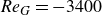
Sketch of our experimental set-up. A falling liquid film of water flows down a glass plate inclined at an angle
 $\beta$
and, after transiting through a protected zone, enters in contact with a counter-current turbulent air flow within a rectangular channel of height
$\beta$
and, after transiting through a protected zone, enters in contact with a counter-current turbulent air flow within a rectangular channel of height
 $H^\star ={13}\,\textrm {mm}$
and width
$H^\star ={13}\,\textrm {mm}$
and width
 $W^\star ={270}\,\textrm {mm}$
. The film surface deformation can be captured with two different cameras, a CCD camera with a line sensor (Basler, Sprint spl 4096) and a CMOS camera with a two-dimensional sensor (Basler, ace acA2440-75uc), both capturing a range of
$W^\star ={270}\,\textrm {mm}$
. The film surface deformation can be captured with two different cameras, a CCD camera with a line sensor (Basler, Sprint spl 4096) and a CMOS camera with a two-dimensional sensor (Basler, ace acA2440-75uc), both capturing a range of
 $x\approx {50}{-}{80}\,\textrm {cm}$
. The photograph shows upward-travelling ripples emanating from the ISW mode.
$x\approx {50}{-}{80}\,\textrm {cm}$
. The photograph shows upward-travelling ripples emanating from the ISW mode.

Spatio-temporal shadowgraphs obtained from new experiments (
 $T\approx {22}\,^\circ\textrm{C}$
) using the set-up of Ishimura et al. (Reference Ishimura, Mergui, Ruyer-Quil and Dietze2023). Falling water film sheared by a counter-current turbulent air flow:
$T\approx {22}\,^\circ\textrm{C}$
) using the set-up of Ishimura et al. (Reference Ishimura, Mergui, Ruyer-Quil and Dietze2023). Falling water film sheared by a counter-current turbulent air flow:
 $H^\star ={13}\,\textrm {mm}$
. Bright contours track spatio-temporal evolution of wave crests. (a–d)
$H^\star ={13}\,\textrm {mm}$
. Bright contours track spatio-temporal evolution of wave crests. (a–d)
 $\beta ={1}^\circ$
,
$\beta ={1}^\circ$
,
 ${\textit{Re}}_{{L}}=103 \pm3$
. (e–h)
${\textit{Re}}_{{L}}=103 \pm3$
. (e–h)
 $\beta ={5}^\circ$
,
$\beta ={5}^\circ$
,
 ${\textit{Re}}_{{L}}=45.3 \pm1.1$
. (a,e) Quiescent gas. (b,f) First evidence of the ISW mode. (c,g) Upward-travelling (in negative
${\textit{Re}}_{{L}}=45.3 \pm1.1$
. (a,e) Quiescent gas. (b,f) First evidence of the ISW mode. (c,g) Upward-travelling (in negative
 $x$
-direction) ripples emanating from the ISW mode overpower Kapitza waves. (d,h) Ripples extend over the entire gas-sheared film surface. (b)
$x$
-direction) ripples emanating from the ISW mode overpower Kapitza waves. (d,h) Ripples extend over the entire gas-sheared film surface. (b)
 ${\textit{Re}}_{{G}}=-2540$
, (c)
${\textit{Re}}_{{G}}=-2540$
, (c)
 ${\textit{Re}}_{{G}}=-3040$
, (d)
${\textit{Re}}_{{G}}=-3040$
, (d)
 ${\textit{Re}}_{{G}}=-3515$
; ( f)
${\textit{Re}}_{{G}}=-3515$
; ( f)
 ${\textit{Re}}_{{G}}=-5200$
, (g)
${\textit{Re}}_{{G}}=-5200$
, (g)
 ${\textit{Re}}_{{G}}=-6620$
, (h)
${\textit{Re}}_{{G}}=-6620$
, (h)
 ${\textit{Re}}_{{G}}=-6760$
.
${\textit{Re}}_{{G}}=-6760$
.

In the current manuscript, we have used the set-up of Ishimura et al. (Reference Ishimura, Mergui, Ruyer-Quil and Dietze2023) to perform additional experiments that focus on characterising the ISW mode. Thereby, we have made the following improvements. First, in addition to a CMOS camera (Basler, ace acA2440-75uc) employed to obtain two-dimensional (2-D) shadowgraphs (see the inset in figure 1), we have employed a CCD camera with a linear sensor (Basler, Sprint spl 4096) to directly obtain highly resolved spatio-temporal recordings of the film surface along the central-axis of the channel across an interval spanning from
 $x^\star ={50}\,\textrm {cm}$
to
$x^\star ={50}\,\textrm {cm}$
to
 $x^\star ={80}\,\textrm {cm}$
, where
$x^\star ={80}\,\textrm {cm}$
, where
 $x$
is the wall-parallel coordinate in streamwise direction (see figure 5). Figure 2 shows typical spatio-temporal shadowgraphs generated from such recordings at constant
$x$
is the wall-parallel coordinate in streamwise direction (see figure 5). Figure 2 shows typical spatio-temporal shadowgraphs generated from such recordings at constant
 ${\textit{Re}}_{{L}}$
. These highly resolved shadowgraphs allow a more precise detection of the onset of upward-travelling ripples. Second, we have varied the gas Reynolds number more finely, to detect more precisely the onset of the ISW mode from the spatio-temporal diagrams. We have determined the critical value of
${\textit{Re}}_{{L}}$
. These highly resolved shadowgraphs allow a more precise detection of the onset of upward-travelling ripples. Second, we have varied the gas Reynolds number more finely, to detect more precisely the onset of the ISW mode from the spatio-temporal diagrams. We have determined the critical value of
 ${\textit{Re}}_{{G}}$
associated with the onset of the ISW mode for inclination angles ranging from
${\textit{Re}}_{{G}}$
associated with the onset of the ISW mode for inclination angles ranging from
 $\beta ={1}^\circ$
to
$\beta ={1}^\circ$
to
 $\beta ={8}^\circ$
. In these experiments, surface waves developed naturally via the amplification of ambient noise.
$\beta ={8}^\circ$
. In these experiments, surface waves developed naturally via the amplification of ambient noise.
Two sets of experiments were performed with distilled water and air at ambient temperatures
 $T\approx {22}\,^\circ\textrm{C}$
(figures 2 and 21
b) and
$T\approx {22}\,^\circ\textrm{C}$
(figures 2 and 21
b) and
 $T\approx {19.5}\,^\circ \textrm {C}$
(figures 3 and 4). The density,
$T\approx {19.5}\,^\circ \textrm {C}$
(figures 3 and 4). The density,
 $\rho _{{L}}$
, and dynamic viscosity,
$\rho _{{L}}$
, and dynamic viscosity,
 $\mu _{{L}}$
, of the liquid were measured as
$\mu _{{L}}$
, of the liquid were measured as
 $\rho _{{L}}={997.8}\,\textrm {kg}\,\textrm {m}^{-3}$
,
$\rho _{{L}}={997.8}\,\textrm {kg}\,\textrm {m}^{-3}$
,
 $\mu _{{L}}={0.97}\,\textrm {mPa s}$
for
$\mu _{{L}}={0.97}\,\textrm {mPa s}$
for
 $T={22}\,^\circ \textrm {C}$
and
$T={22}\,^\circ \textrm {C}$
and
 $\rho _{{L}}={998.2}\,\textrm {kg}\,\textrm {m}^{-3}$
,
$\rho _{{L}}={998.2}\,\textrm {kg}\,\textrm {m}^{-3}$
,
 $\mu _{{L}}={1.02}\,\textrm {mPa s}$
for
$\mu _{{L}}={1.02}\,\textrm {mPa s}$
for
 $T={19.5}\,^\circ \textrm {C}$
. The surface tension,
$T={19.5}\,^\circ \textrm {C}$
. The surface tension,
 $\sigma$
, was measured as
$\sigma$
, was measured as
 $\sigma ={72.2}\,\textrm {mN}\,\textrm {m}^{-1}$
for
$\sigma ={72.2}\,\textrm {mN}\,\textrm {m}^{-1}$
for
 $T={22}\,^\circ \textrm {C}$
and interpolated from Vargaftik, Volkov & Voljak (Reference Vargaftik, Volkov and Voljak1983) as
$T={22}\,^\circ \textrm {C}$
and interpolated from Vargaftik, Volkov & Voljak (Reference Vargaftik, Volkov and Voljak1983) as
 $\sigma ={72.83}\,\textrm {mN}\,\textrm {m}^{-1}$
for
$\sigma ={72.83}\,\textrm {mN}\,\textrm {m}^{-1}$
for
 $T={19.5}\,^\circ \textrm {C}$
. The data obtained from these experiments will be compared with our linear stability calculations (see figures 4
b and 21
b). The shadowgraphs in figure 2 correspond to two typical experimental runs, which were used to identify the onset of the ISW mode by increasing the counter-current gas flow rate at fixed
$T={19.5}\,^\circ \textrm {C}$
. The data obtained from these experiments will be compared with our linear stability calculations (see figures 4
b and 21
b). The shadowgraphs in figure 2 correspond to two typical experimental runs, which were used to identify the onset of the ISW mode by increasing the counter-current gas flow rate at fixed
 $\beta$
and
$\beta$
and
 ${\textit{Re}}_{{L}}$
. Two series are represented:
${\textit{Re}}_{{L}}$
. Two series are represented:
 ${{\textit{Re}}_{{L}}}={103}$
at
${{\textit{Re}}_{{L}}}={103}$
at
 $\beta ={1}^\circ$
(figures 2
a–2
d) and
$\beta ={1}^\circ$
(figures 2
a–2
d) and
 ${{\textit{Re}}_{{L}}}={45.3}$
at
${{\textit{Re}}_{{L}}}={45.3}$
at
 $\beta ={5}^\circ$
(figures 2
e–2
h). Figures 2(a) and 2(e) correspond to the reference configuration of a quiescent gas, where only downward-travelling long waves resulting from the Kapitza instability develop. In figure 2(a), the wave amplitude is too weak to generate shadows that can be detected by our camera. By contrast, in figure 2(e), wave crests associated with Kapitza waves are clearly visible via bright contours that possess a negative slope, i.e. these waves move in positive
$\beta ={5}^\circ$
(figures 2
e–2
h). Figures 2(a) and 2(e) correspond to the reference configuration of a quiescent gas, where only downward-travelling long waves resulting from the Kapitza instability develop. In figure 2(a), the wave amplitude is too weak to generate shadows that can be detected by our camera. By contrast, in figure 2(e), wave crests associated with Kapitza waves are clearly visible via bright contours that possess a negative slope, i.e. these waves move in positive
 $x$
-direction with increasing time. Intersections of crest contours evidence noise-driven wave coalescence events. In all other panels, the falling liquid film is subject to a counter-current air flow.
$x$
-direction with increasing time. Intersections of crest contours evidence noise-driven wave coalescence events. In all other panels, the falling liquid film is subject to a counter-current air flow.
Experiments using CMOS camera with two-dimensional sensor (
 $T\approx {19.5}\,^\circ \textrm {C}$
). Shadowgraphs showing upward-travelling ripples. Conditions similar to figures 2(c) and 2(d):
$T\approx {19.5}\,^\circ \textrm {C}$
). Shadowgraphs showing upward-travelling ripples. Conditions similar to figures 2(c) and 2(d):
 $\beta =1^\circ$
,
$\beta =1^\circ$
,
 $H^\star$
= 13 mm,
$H^\star$
= 13 mm,
 ${\textit{Re}}_{{L}}=100\pm 3$
. (a)
${\textit{Re}}_{{L}}=100\pm 3$
. (a)
 ${\textit{Re}}_{{G}}=-3040$
(very close to ISW threshold); (b)
${\textit{Re}}_{{G}}=-3040$
(very close to ISW threshold); (b)
 ${\textit{Re}}_{{G}}=-3515$
.
${\textit{Re}}_{{G}}=-3515$
.

Frequency of upward-travelling ripples. Experiments with CCI probe for conditions according to figure 3(b). (a) Film thickness time trace obtained with 400 Hz acquisition frequency; (b) frequency spectrum obtained by averaging 20 film thickness time-trace signals of 25 s each. The frequency has been normalised with the linearly most-amplified frequency,
 $f^\star _{\textit{max}}={7.3}\,\textrm {Hz}$
, obtained from a spatial linear stability calculation, and
$f^\star _{\textit{max}}={7.3}\,\textrm {Hz}$
, obtained from a spatial linear stability calculation, and
 $\hat {h}_m$
denotes the amplitude of a Fourier mode with frequency
$\hat {h}_m$
denotes the amplitude of a Fourier mode with frequency
 $f^\star _m=m\Delta f^\star$
, where
$f^\star _m=m\Delta f^\star$
, where
 $m\in \mathbb{Z}$
and
$m\in \mathbb{Z}$
and
 $\Delta f^\star ={0.04}\,\textrm {Hz}$
.
$\Delta f^\star ={0.04}\,\textrm {Hz}$
.

Falling liquid film (subscript
 ${L}$
) on an inclined wall subject to a counter-current turbulent gas flow (subscript
${L}$
) on an inclined wall subject to a counter-current turbulent gas flow (subscript
 ${G}$
). The flow is confined by an upper wall at
${G}$
). The flow is confined by an upper wall at
 $y^\star$
=
$y^\star$
=
 $H^\star$
(not shown). In the linear limit, the gas flow is symmetrical about
$H^\star$
(not shown). In the linear limit, the gas flow is symmetrical about
 $y^\star$
=
$y^\star$
=
 $D^\star$
=
$D^\star$
=
 $(H^\star +h_0^\star )/2$
. Magenta dashed lines illustrate the orthogonal curvilinear coordinate system used for the gas, (
$(H^\star +h_0^\star )/2$
. Magenta dashed lines illustrate the orthogonal curvilinear coordinate system used for the gas, (
 $\eta$
,
$\eta$
,
 $\xi$
), where
$\xi$
), where
 $\eta$
=
$\eta$
=
 $\underline{y}d_0/d$
. The subscript
$\underline{y}d_0/d$
. The subscript
 $0$
denotes the primary flow.
$0$
denotes the primary flow.

We start by discussing figures 2(b)–2(d), which correspond to
 $\beta ={1}^\circ$
(see also figure 3, which will be discussed later). In figure 2(b), the value of
$\beta ={1}^\circ$
(see also figure 3, which will be discussed later). In figure 2(b), the value of
 ${\textit{Re}}_{{G}}$
is slightly beyond the threshold of the ISW mode, i.e. the first evidence of upward-travelling ripples is detectable. In particular, wave crest contours with a positive slope are observed in the lower half of figure 2(b) (
${\textit{Re}}_{{G}}$
is slightly beyond the threshold of the ISW mode, i.e. the first evidence of upward-travelling ripples is detectable. In particular, wave crest contours with a positive slope are observed in the lower half of figure 2(b) (
 $x^\star \gt {70}\,\textrm {cm}$
), evidencing wave fronts that move in negative
$x^\star \gt {70}\,\textrm {cm}$
), evidencing wave fronts that move in negative
 $x$
-direction with increasing time. These upward-travelling ripples coexist with downward-travelling Kapitza waves, as evidenced by the bright contours with positive slope in the top half of the panel. Upon increasing the counter-current gas flow rate further, ripples emanating from the ISW mode progressively invade the domain and eventually overpower the Kapiza waves (figure 2
d,
$x$
-direction with increasing time. These upward-travelling ripples coexist with downward-travelling Kapitza waves, as evidenced by the bright contours with positive slope in the top half of the panel. Upon increasing the counter-current gas flow rate further, ripples emanating from the ISW mode progressively invade the domain and eventually overpower the Kapiza waves (figure 2
d,
 ${{\textit{Re}}_{{G}}}=-3515$
). This can be understood via figure 11 of Ishimura et al. (Reference Ishimura, Mergui, Ruyer-Quil and Dietze2023), where it was shown for the same conditions that the counter-current gas flow exerts a stabilising effect on the Kapitza instability mode, eventually suppressing it at
${{\textit{Re}}_{{G}}}=-3515$
). This can be understood via figure 11 of Ishimura et al. (Reference Ishimura, Mergui, Ruyer-Quil and Dietze2023), where it was shown for the same conditions that the counter-current gas flow exerts a stabilising effect on the Kapitza instability mode, eventually suppressing it at
 ${{\textit{Re}}_{{G}}}=-3400$
. By contrast, the appearance of Kapitza waves between figures 2(a) (aerostatic) and 2(b) (
${{\textit{Re}}_{{G}}}=-3400$
. By contrast, the appearance of Kapitza waves between figures 2(a) (aerostatic) and 2(b) (
 ${{\textit{Re}}_{{G}}}=-2540$
) can be explained by an increased noise level when the falling liquid film is sheared by a turbulent counter-current gas flow.
${{\textit{Re}}_{{G}}}=-2540$
) can be explained by an increased noise level when the falling liquid film is sheared by a turbulent counter-current gas flow.
Similar observations are made for the larger inclination angle,
 $\beta ={5}^\circ$
(figures 2
f–2
h). However, in this case, Kapitza waves reach a developed nonlinear state within the protected zone of the experimental set-up, before coming into contact with the counter-current gas flow. Due to this, the onset of the ISW instability manifests itself in another way. As shown in figure 2( f), which corresponds to slightly supercritical conditions in terms of the ISW instability, the wave crest contours of the Kapitza waves are distorted by slight kinks, which evolve into positively sloped wave contours associated with upward-travelling ripples as the counter-current gas flow rate is increased (figure 2
g). That the first manifestations of the ISW mode occur on the wave humps of the nonlinear Kapitza waves is due to the higher local confinement of the gas flow there. We will see in § 4.2 that the critical value of
$\beta ={5}^\circ$
(figures 2
f–2
h). However, in this case, Kapitza waves reach a developed nonlinear state within the protected zone of the experimental set-up, before coming into contact with the counter-current gas flow. Due to this, the onset of the ISW instability manifests itself in another way. As shown in figure 2( f), which corresponds to slightly supercritical conditions in terms of the ISW instability, the wave crest contours of the Kapitza waves are distorted by slight kinks, which evolve into positively sloped wave contours associated with upward-travelling ripples as the counter-current gas flow rate is increased (figure 2
g). That the first manifestations of the ISW mode occur on the wave humps of the nonlinear Kapitza waves is due to the higher local confinement of the gas flow there. We will see in § 4.2 that the critical value of
 $|{{\textit{Re}}_{{G}}}|$
for the linear onset of the ISW mode decreases with increasing confinement (figure 19).
$|{{\textit{Re}}_{{G}}}|$
for the linear onset of the ISW mode decreases with increasing confinement (figure 19).
Because the experimental onset of upward-travelling ripples may be observed on an already nonlinear train of Kapitza waves, depending on the set of parameters (
 $\beta$
,
$\beta$
,
 ${\textit{Re}}_{{L}}$
), one should not expect agreement always with the linear onset of the ISW mode determined via our spatio-temporal stability calculations. However, for the conditions used in our experiments, we observe very good agreement (see e.g. figure 21
b), as the amplitude of nonlinear Kapitza waves is rather small compared with the channel height, and, thus, the variation in local relative gas confinement across a Kapitza wave is rather weak. For example, based on CCI measurements, the typical height of a Kapitza wave for the conditions in figure 2( f) at the onset of the ISW mode is
${\textit{Re}}_{{L}}$
), one should not expect agreement always with the linear onset of the ISW mode determined via our spatio-temporal stability calculations. However, for the conditions used in our experiments, we observe very good agreement (see e.g. figure 21
b), as the amplitude of nonlinear Kapitza waves is rather small compared with the channel height, and, thus, the variation in local relative gas confinement across a Kapitza wave is rather weak. For example, based on CCI measurements, the typical height of a Kapitza wave for the conditions in figure 2( f) at the onset of the ISW mode is
 $h_{\textit{max}}^\star \approx {1}\,\textrm {mm}$
, and the typical thickness of the residual film in between wave humps is
$h_{\textit{max}}^\star \approx {1}\,\textrm {mm}$
, and the typical thickness of the residual film in between wave humps is
 $h_{{res}}^\star \approx {0.3}\,\textrm {mm}$
. Thus, the gas layer thickness,
$h_{{res}}^\star \approx {0.3}\,\textrm {mm}$
. Thus, the gas layer thickness,
 $H^\star {-}h^\star$
, varies by only 5 % of the channel height,
$H^\star {-}h^\star$
, varies by only 5 % of the channel height,
 $H^\star ={13}\,\textrm {mm}$
. For larger values of
$H^\star ={13}\,\textrm {mm}$
. For larger values of
 ${\textit{Re}}_{{L}}$
and/or
${\textit{Re}}_{{L}}$
and/or
 $\beta$
, this variation increases, and comparison between experiment and linear stability calculations is no longer appropriate. Consequently, we have only considered
$\beta$
, this variation increases, and comparison between experiment and linear stability calculations is no longer appropriate. Consequently, we have only considered
 ${\textit{Re}}_{{L}}$
–
${\textit{Re}}_{{L}}$
–
 $\beta$
parameter pairs where the variation in local confinement is less than 7 % in the experiments used to validate our linear stability calculations of the ISW instability threshold (figure 21
b).
$\beta$
parameter pairs where the variation in local confinement is less than 7 % in the experiments used to validate our linear stability calculations of the ISW instability threshold (figure 21
b).
The main linear stability calculations presented in the current manuscript are based on a two-dimensional formulation. Thus, the question arises as to whether the upward-travelling ripples produced by the ISW mode are indeed two-dimensional. Figures 3(a) and 3(b) represent two-dimensional shadowgraphs captured with our CMOS camera for the conditions in figures 2(c) and 2(d). A similar snapshot is shown as an inset in figure 1. These experiments, performed at a very low inclination angle,
 $\beta ={1}^\circ$
, are favourable to the ISW mode, because Kapitza waves, which are prone to a gas-aided secondary three-dimensional instability mode (Kofman et al. Reference Kofman, Mergui and Ruyer-Qui2014, Reference Kofman, Mergui and Ruyer-Quil2017), entirely disappear upon increasing the counter-current gas flow rate (figure 2
d). Figure 3(a) corresponds to conditions only slightly above the onset of upward-travelling ripples and, thus, the shadows of the wave fronts are quite faint. Nonetheless, it can be observed that the fronts are more or less two-dimensional, even though three-dimensional defects are also visible. The latter become more pronounced in figure 3(b), which corresponds to a larger value of
$\beta ={1}^\circ$
, are favourable to the ISW mode, because Kapitza waves, which are prone to a gas-aided secondary three-dimensional instability mode (Kofman et al. Reference Kofman, Mergui and Ruyer-Qui2014, Reference Kofman, Mergui and Ruyer-Quil2017), entirely disappear upon increasing the counter-current gas flow rate (figure 2
d). Figure 3(a) corresponds to conditions only slightly above the onset of upward-travelling ripples and, thus, the shadows of the wave fronts are quite faint. Nonetheless, it can be observed that the fronts are more or less two-dimensional, even though three-dimensional defects are also visible. The latter become more pronounced in figure 3(b), which corresponds to a larger value of
 $|{Re_G}|$
. At present, it is not possible to determine whether the three-dimensional features are due to linear or nonlinear growth mechanisms. Preliminary three-dimensional stability calculations for the larger inclination angle,
$|{Re_G}|$
. At present, it is not possible to determine whether the three-dimensional features are due to linear or nonlinear growth mechanisms. Preliminary three-dimensional stability calculations for the larger inclination angle,
 $\beta ={5}^\circ$
, which are presented in Appendix A and discussed in § 3, suggest that the ISW threshold may be slightly lower for three-dimensional perturbations than for two-dimensional ones. However, the shift of the critical gas Reynolds number magnitude observed in these calculations is of the order of 4 %, which is within the error bar of our experiments, and, thus, cannot be resolved experimentally. Further, our preliminary calculations are based on an equivalent two-dimensional formulation that can only be obtained by neglecting the perturbation of the turbulent viscosity and, thus, need to be confirmed with full three-dimensional calculations. These are outside the scope of the current manuscript. Thus, for the time being, and following Vellingiri et al. (Reference Vellingiri, Tseluiko and Kalliadasis2015) and Schmidt et al. (Reference Schmidt, Náraigh, Lucquiaud and Valluri2016), we rely on our two-dimensional stability calculations, which are in very good agreement with our experiments, e.g. they accurately predict the threshold of the ISW mode (see figure 21
b, which will be discussed in § 4). Very good agreement is also observed between the dominant frequency of the upward travelling ripples in our experiments and the linearly most-amplified frequency,
$\beta ={5}^\circ$
, which are presented in Appendix A and discussed in § 3, suggest that the ISW threshold may be slightly lower for three-dimensional perturbations than for two-dimensional ones. However, the shift of the critical gas Reynolds number magnitude observed in these calculations is of the order of 4 %, which is within the error bar of our experiments, and, thus, cannot be resolved experimentally. Further, our preliminary calculations are based on an equivalent two-dimensional formulation that can only be obtained by neglecting the perturbation of the turbulent viscosity and, thus, need to be confirmed with full three-dimensional calculations. These are outside the scope of the current manuscript. Thus, for the time being, and following Vellingiri et al. (Reference Vellingiri, Tseluiko and Kalliadasis2015) and Schmidt et al. (Reference Schmidt, Náraigh, Lucquiaud and Valluri2016), we rely on our two-dimensional stability calculations, which are in very good agreement with our experiments, e.g. they accurately predict the threshold of the ISW mode (see figure 21
b, which will be discussed in § 4). Very good agreement is also observed between the dominant frequency of the upward travelling ripples in our experiments and the linearly most-amplified frequency,
 $f_{\textit{max}}$
, obtained from a spatial linear stability calculation (as we will show, the ISW mode is upward-convective). Following Valluri et al. (Reference Valluri, Náraigh, Ding and Spelt2010), this is shown in figure 4(b), representing the frequency spectrum of the experimental wave profile represented in figure 4(a) and corresponding to the parameters in figure 3(b), whereby the frequency,
$f_{\textit{max}}$
, obtained from a spatial linear stability calculation (as we will show, the ISW mode is upward-convective). Following Valluri et al. (Reference Valluri, Náraigh, Ding and Spelt2010), this is shown in figure 4(b), representing the frequency spectrum of the experimental wave profile represented in figure 4(a) and corresponding to the parameters in figure 3(b), whereby the frequency,
 $f^\star$
, has been normalised with
$f^\star$
, has been normalised with
 $f_{\textit{max}}^\star ={7.3}\,\textrm {Hz}$
. The peak of the spectrum is observed at
$f_{\textit{max}}^\star ={7.3}\,\textrm {Hz}$
. The peak of the spectrum is observed at
 $f^\star$
/
$f^\star$
/
 $f_{\textit{max}}^\star {\approx }1$
.
$f_{\textit{max}}^\star {\approx }1$
.
3. Orr–Sommerfeld spatio-temporal linear stability calculations
We consider the two-dimensional configuration sketched in figure 5. A laminar falling liquid film (subscript L) of thickness,
 $h$
, and flow rate (per unit width),
$h$
, and flow rate (per unit width),
 $q_{{L}}$
, with constant density,
$q_{{L}}$
, with constant density,
 $\rho _{{L}}$
, dynamic viscosity,
$\rho _{{L}}$
, dynamic viscosity,
 $\mu _{{L}}$
, and surface tension,
$\mu _{{L}}$
, and surface tension,
 $\sigma$
, flows down a plane inclined at an angle,
$\sigma$
, flows down a plane inclined at an angle,
 $\beta$
, and is sheared by a turbulent counter-current gas flow (subscript G) of flow rate,
$\beta$
, and is sheared by a turbulent counter-current gas flow (subscript G) of flow rate,
 $q_{{G}}$
, with constant density,
$q_{{G}}$
, with constant density,
 $\rho _{{G}}$
, and dynamic viscosity,
$\rho _{{G}}$
, and dynamic viscosity,
 $\mu _{{G}}$
. Both fluids are considered Newtonian. The gas is confined by an upper wall at
$\mu _{{G}}$
. Both fluids are considered Newtonian. The gas is confined by an upper wall at
 $y^\star$
=
$y^\star$
=
 $H^\star$
, which is not shown. We assume that the superficial gas velocity,
$H^\star$
, which is not shown. We assume that the superficial gas velocity,
 $\mathcal{U}_{{G}}$
=
$\mathcal{U}_{{G}}$
=
 $q_{{{G}} 0}^\star$
/
$q_{{{G}} 0}^\star$
/
 $H^\star$
, is much greater than the superficial liquid velocity,
$H^\star$
, is much greater than the superficial liquid velocity,
 $\mathcal{U}_{{L}}$
=
$\mathcal{U}_{{L}}$
=
 $q_{{{L}} 0}^\star$
/
$q_{{{L}} 0}^\star$
/
 $H^\star$
, where, and throughout the manuscript, the star symbol and calligraphic typeface denote dimensional quantities, and the subscript
$H^\star$
, where, and throughout the manuscript, the star symbol and calligraphic typeface denote dimensional quantities, and the subscript
 $0$
denotes the primary flow. Thus, the liquid–gas interface is considered immobile and rigid from the point of view of the gas, and the gas-side problem can be solved independently for a given film height profile,
$0$
denotes the primary flow. Thus, the liquid–gas interface is considered immobile and rigid from the point of view of the gas, and the gas-side problem can be solved independently for a given film height profile,
 $h(x,t)$
. Due to this assumption, and because we are only interested in the linear response of the system, the gas flow can be considered symmetrical with respect to
$h(x,t)$
. Due to this assumption, and because we are only interested in the linear response of the system, the gas flow can be considered symmetrical with respect to
 $y^\star$
=
$y^\star$
=
 $D^\star$
=
$D^\star$
=
 $(H^\star +h_0^\star )/2$
, and only the bottom half of the gas layer needs to be represented. The effect of the gas on the liquid film is represented via the tangential and normal gas stresses,
$(H^\star +h_0^\star )/2$
, and only the bottom half of the gas layer needs to be represented. The effect of the gas on the liquid film is represented via the tangential and normal gas stresses,
 $T_{{G}}$
and
$T_{{G}}$
and
 $P_{{G}}$
, acting at the liquid–gas interface. Thus, we neglect normal viscous gas stresses. Figure 6 represents typical velocity profiles of the primary flow, which will be further discussed in §§ 3.1 and 3.2.
$P_{{G}}$
, acting at the liquid–gas interface. Thus, we neglect normal viscous gas stresses. Figure 6 represents typical velocity profiles of the primary flow, which will be further discussed in §§ 3.1 and 3.2.
Primary-flow streamwise velocity profiles in the (a) liquid and (b) gas for
 $H^\star ={13}\,\textrm {mm}$
,
$H^\star ={13}\,\textrm {mm}$
,
 $\beta ={5}^\circ$
,
$\beta ={5}^\circ$
,
 ${\textit{Re}}_{{L}}$
= 43.1,
${\textit{Re}}_{{L}}$
= 43.1,
 $T_{{{G}}0}^\star ={478}\,\textrm {N}\,\textrm {m}^{-2}$
. Velocities are normalised with the respective maximum gas velocity. (a) Liquid-side velocity profiles; (b) gas-side velocity profiles at equivalent tangential gas shear stress. Solid line, solution for turbulent gas flow at
$T_{{{G}}0}^\star ={478}\,\textrm {N}\,\textrm {m}^{-2}$
. Velocities are normalised with the respective maximum gas velocity. (a) Liquid-side velocity profiles; (b) gas-side velocity profiles at equivalent tangential gas shear stress. Solid line, solution for turbulent gas flow at
 ${\textit{Re}}_{{G}}=-1800$
; dashed line, solution for laminar gas flow at
${\textit{Re}}_{{G}}=-1800$
; dashed line, solution for laminar gas flow at
 ${\textit{Re}}_{{G}}=-4101$
.
${\textit{Re}}_{{G}}=-4101$
.

This weakly coupled approach was introduced by Tseluiko & Kalliadasis (Reference Tseluiko and Kalliadasis2011) and we have shown that it allows to accurately predict the linear response of a gas-sheared falling liquid film in comparison with experiments (Ishimura et al. Reference Ishimura, Mergui, Ruyer-Quil and Dietze2023). In our linear stability analysis, the assumption
 $\mathcal{U}_{{G}}\gg \mathcal{U}_{{L}}$
implies that temporal derivatives vanish from the linearised gas-side problem and linear growth occurs only via the liquid–gas interface. Thus, the liquid- and gas-side instability problems can be solved sequentially instead of simultaneously, i.e. for a given interface perturbation with wavenumber,
$\mathcal{U}_{{G}}\gg \mathcal{U}_{{L}}$
implies that temporal derivatives vanish from the linearised gas-side problem and linear growth occurs only via the liquid–gas interface. Thus, the liquid- and gas-side instability problems can be solved sequentially instead of simultaneously, i.e. for a given interface perturbation with wavenumber,
 $k$
, we calculate the linear response of the gas flow in terms of
$k$
, we calculate the linear response of the gas flow in terms of
 $T_{{G}}$
and
$T_{{G}}$
and
 $P_{{G}}$
. Subsequently, we use the thus obtained linear gas stress perturbations to calculate the linear response of the liquid film.
$P_{{G}}$
. Subsequently, we use the thus obtained linear gas stress perturbations to calculate the linear response of the liquid film.
Our main stability calculations are based on a two-dimensional formulation, which we have justified in §§ 1 and 2. For futher details, including a preliminary three-dimensional calculation, the reader is referred to Appendix A.
3.1. Liquid-side description
The liquid film is governed by the dimensionless continuity and Navier–Stokes equations written in the Cartesian coordinates,
 $x$
and
$x$
and
 $y$
,
$y$
,
 \begin{align} \partial _xu_{{L}} + \partial _yv_{{L}} &= 0, \end{align}
 \begin{align} (\partial _tu_{{L}} + u_{{L}}\partial _xu_{{L}} + v_{{L}}\partial _yu_{{L}})&=- \partial _xp_{{L}} + \frac {1}{{\textit{Re}}_{{L}}}(\partial _{xx}u_{{L}} + \partial _{yy}u_{{L}}) + \frac {\sin (\beta )}{{\textit{Fr}} ^2}, \end{align}
 \begin{align} (\partial _tv_{{L}} + u_{{L}}\partial _xv_{{L}} + v_{{L}}\partial _yv_{{L}}) &= - \partial _yp_{{L}} + \frac {1}{{\textit{Re}}_{{L}}}(\partial _{xx}v_{{L}} + \partial _{yy}v_{{L}}) - \frac {\cos (\beta )}{{\textit{Fr}} ^2}, \end{align}
where
 $p_{{L}}$
denotes the liquid pressure, and
$p_{{L}}$
denotes the liquid pressure, and
 ${\textit{Re}}_{{L}}$
=
${\textit{Re}}_{{L}}$
=
 $\rho _{{L}}\mathcal{U}_{{L}}\mathcal{L}$
/
$\rho _{{L}}\mathcal{U}_{{L}}\mathcal{L}$
/
 $\mu _{{L}}$
and
$\mu _{{L}}$
and
 ${\textit{Fr}}$
=
${\textit{Fr}}$
=
 $\mathcal{U}_{{L}}$
/
$\mathcal{U}_{{L}}$
/
 $\sqrt {\mathcal{L}g}$
denote the liquid Reynolds number and Froude number, and where we have applied the following scaling:
$\sqrt {\mathcal{L}g}$
denote the liquid Reynolds number and Froude number, and where we have applied the following scaling:
 \begin{align} u_{{L}}=\frac {u^\star _{{L}}}{\mathcal{U}_{{L}}},\quad v_{{L}}=\frac {v_{{L}}^\star }{\mathcal{U}_{{L}}},\quad x=\frac {x^\star }{\mathcal{L}},\quad y=\frac {y^\star }{\mathcal{L}},\quad t= t^\star \,\frac {\mathcal{U}_{{L}}}{\mathcal{L}}, \quad p_{{L}}=\frac {p_{{L}}^\star }{\rho _{{L}}\mathcal{U}_{{L}}^2}. \end{align}
We choose the channel height,
 $H^\star$
, as the length scale, i.e.
$H^\star$
, as the length scale, i.e.
 $\mathcal{L}$
=
$\mathcal{L}$
=
 $H^\star$
, and the liquid superficial velocity as the velocity scale, i.e.
$H^\star$
, and the liquid superficial velocity as the velocity scale, i.e.
 $\mathcal{U}_{{L}}$
=
$\mathcal{U}_{{L}}$
=
 $q^\star _{{{L}} 0}$
/
$q^\star _{{{L}} 0}$
/
 $H^\star$
. The system is closed with the boundary conditions at
$H^\star$
. The system is closed with the boundary conditions at
 $y$
= 0,
$y$
= 0,
 \begin{align} u_{{L}}=v_{{L}}=0, \end{align}
the kinematic condition at
 $y$
=
$y$
=
 $h$
,
$h$
,
 \begin{align} {v_{{L}}}=\partial _{t} h+{u_{{L}}} \partial _{x} h, \end{align}
and the inter-phase stress coupling conditions at
 $y$
=
$y$
=
 $h$
,
$h$
,
 \begin{align}&\qquad -\frac {1}{1+ \partial _xh^2}\left \{ (\partial _xh^2-1)(\partial _yu_{{L}}+\partial _xv_{{L}})+4 \partial _xh \partial _xu_{{L}}\right \}={\varPi _\mu \varPi _u} T_{{G}}, \end{align}
 \begin{align} P_{{L}} &- \frac {2}{1+ \partial _xh^2}\frac {1}{{\textit{Re}}_{{L}}}( \partial _xh^2 \partial _xu_{{L}} - \partial _xh \partial _xv_{{L}} - \partial _xu_{{L}} - \partial _xh\partial _yu_{{L}})- {\textit{We}} \frac {\partial _{xx}h}{(1+\partial _xh^2)^{3/2}}\nonumber \\ &\quad= \frac {1}{{\textit{Re}}_{{G}}} {\varPi _\rho \varPi _u^2} P_{{G}}, \end{align}
where
 $P_{{L}}$
denotes the liquid pressure at the liquid–gas interface and
$P_{{L}}$
denotes the liquid pressure at the liquid–gas interface and
 ${\textit{We}}$
=
${\textit{We}}$
=
 $\sigma$
/
$\sigma$
/
 $\rho _{{L}}$
/
$\rho _{{L}}$
/
 $\mathcal{L}$
/
$\mathcal{L}$
/
 $\mathcal{U}_{{L}}^2$
denotes the Weber number. We also introduce the Kapitza number,
$\mathcal{U}_{{L}}^2$
denotes the Weber number. We also introduce the Kapitza number,
 ${\textit{Ka}}$
=
${\textit{Ka}}$
=
 $\sigma /\rho _{{L}}/g^{1/3}/\nu _{{L}}^{4/3}$
, which is independent of the chosen scaling. The liquid–gas coupling is applied through the interfacial gas stresses,
$\sigma /\rho _{{L}}/g^{1/3}/\nu _{{L}}^{4/3}$
, which is independent of the chosen scaling. The liquid–gas coupling is applied through the interfacial gas stresses,
 $T_{{G}}$
and
$T_{{G}}$
and
 $P_{{G}}$
, which are scaled as follows:
$P_{{G}}$
, which are scaled as follows:
 \begin{equation} T_{{G}}=\frac {\mathcal{L}}{\mu _{{G}} \mathcal{U}_{{G}}}T_{{G}}^\star ,\quad P_{{G}}=\frac {\mathcal{L}}{\mu _{{G}} \mathcal{U}_{{G}}}P_{{G}}^\star , \end{equation}
where
 $\mathcal{U}_{{G}}$
denotes the gas-side velocity scale, which will be defined in § 3.2. As a result, the gas Reynolds number,
$\mathcal{U}_{{G}}$
denotes the gas-side velocity scale, which will be defined in § 3.2. As a result, the gas Reynolds number,
 ${\textit{Re}}_{{G}}$
=
${\textit{Re}}_{{G}}$
=
 $\rho _{{G}}\mathcal{U}_{{G}}\mathcal{L}$
/
$\rho _{{G}}\mathcal{U}_{{G}}\mathcal{L}$
/
 $\mu _{{G}}$
, the velocity scale ratio,
$\mu _{{G}}$
, the velocity scale ratio,
 $\varPi _u$
=
$\varPi _u$
=
 $\mathcal{U}_{{G}}$
/
$\mathcal{U}_{{G}}$
/
 $\mathcal{U}_{{L}}$
, and the viscosity and density ratios,
$\mathcal{U}_{{L}}$
, and the viscosity and density ratios,
 $\varPi _\mu$
=
$\varPi _\mu$
=
 $\mu _{{G}}$
/
$\mu _{{G}}$
/
 $\mu _{{L}}$
and
$\mu _{{L}}$
and
 $\varPi _\rho$
=
$\varPi _\rho$
=
 $\rho _{{G}}$
/
$\rho _{{G}}$
/
 $\rho _{{L}}$
, enter (3.1g
) and (3.1h
).
$\rho _{{L}}$
, enter (3.1g
) and (3.1h
).
The primary flow in the liquid film is obtained by solving (3.1) in the limit of fully developed conditions (figure 6 a),
 \begin{align} u_{{{L}} 0}&=\frac {1}{2}{\textit{Re}}_{{L}}\left \{\varPi _\rho \partial _xP_{{{G}} 0}-\frac {\sin \left (\beta \right )}{{\textit{Fr}}^2}\right \}\left (y^2-2yh_0\right )+{\varPi _\mu \varPi _u}T_{{{G}} 0}\,y, \end{align}
 \begin{align} \partial _y p_{{{L}} 0}&=-\frac {\cos \left (\beta \right )}{{\textit{Fr}}^2}. \end{align}
Next, we recast (3.1) in terms of the stream function,
 $\varPhi$
,
$\varPhi$
,
 \begin{gather} u_{{L}}=\partial _{y}\varPhi ,\quad v_{{L}}=-\partial _{x}\varPhi , \end{gather}
and perturb the system around the primary flow (3.3) via
 \begin{align}&\qquad h=h_0+\check {h}=h_0+\hat {h}\exp \left \{i\left (kx-t\left (\omega +k V_{\textit{ray}}\right )\right )\right \}\!, \end{align}
 \begin{align}&\quad \varPhi =\varPhi _0+\check {\varPhi }=\varPhi _0+\phi (y)\exp \left \{i\left (kx-t\left (\omega +k V_{\textit{ray}}\right )\right )\right \}\!, \end{align}
 \begin{align}& p_{{L}}=p_{{{L}} 0}+\check {p}_{{L}}=p_{{{L}} 0}+\hat {p}_{{L}}(y)\exp \left \{i\left (kx-t\left (\omega +k V_{\textit{ray}}\right )\right )\right \}\!, \end{align}
where the wave number,
 $k$
=
$k$
=
 $k_r$
+
$k_r$
+
 $ik_i$
, and the angular frequency,
$ik_i$
, and the angular frequency,
 $\omega$
=
$\omega$
=
 $\omega _r$
+
$\omega _r$
+
 $i\omega _i$
, are assumed complex, with
$i\omega _i$
, are assumed complex, with
 $i$
=
$i$
=
 $\sqrt {-1}$
and
$\sqrt {-1}$
and
 $k_r,k_i,\omega _r,\omega _i\in \mathbb{R}$
, and where we have introduced the ray velocity,
$k_r,k_i,\omega _r,\omega _i\in \mathbb{R}$
, and where we have introduced the ray velocity,
 $V_{\textit{ray}}\in \mathbb{R}$
, following standard procedure in spatio-temporal stability analysis (Huerre & Monkewitz Reference Huerre and Monkewitz1990; Brevdo et al. Reference Brevdo, Laure, Dias and Bridges1999). This velocity corresponds to the speed of a moving observer contemplating the spatio-temporal evolution of the perturbation. Consequently, the temporal growth rate,
$V_{\textit{ray}}\in \mathbb{R}$
, following standard procedure in spatio-temporal stability analysis (Huerre & Monkewitz Reference Huerre and Monkewitz1990; Brevdo et al. Reference Brevdo, Laure, Dias and Bridges1999). This velocity corresponds to the speed of a moving observer contemplating the spatio-temporal evolution of the perturbation. Consequently, the temporal growth rate,
 $\omega _i$
, and the wave speed,
$\omega _i$
, and the wave speed,
 \begin{equation} c=\frac {\omega }{k}, \end{equation}
with
 $c\in \mathbb{C}$
, are defined in a reference frame moving with
$c\in \mathbb{C}$
, are defined in a reference frame moving with
 $V_{\textit{ray}}$
. For an instability mode that grows only spatially in the laboratory referenced frame, we have
$V_{\textit{ray}}$
. For an instability mode that grows only spatially in the laboratory referenced frame, we have
 $-k_i\gt 0$
and
$-k_i\gt 0$
and
 $\omega _i+k_iV_{\textit{ray}}$
= 0. Thus, the temporal growth rate detected by the moving observer,
$\omega _i+k_iV_{\textit{ray}}$
= 0. Thus, the temporal growth rate detected by the moving observer,
 $\omega _i$
, will depend on the ray velocity,
$\omega _i$
, will depend on the ray velocity,
 $V_{\textit{ray}}$
, and the spatial growth rate,
$V_{\textit{ray}}$
, and the spatial growth rate,
 $-k_i$
.
$-k_i$
.
Next, we linearise the perturbed governing equations in terms of the perturbation increments,
 $\check {h}$
,
$\check {h}$
,
 $\check {p}_{{L}}$
and
$\check {p}_{{L}}$
and
 $\check {\varPhi }$
, yielding the liquid-side Orr–Sommerfeld equation,
$\check {\varPhi }$
, yielding the liquid-side Orr–Sommerfeld equation,
 \begin{align} \phi ^{iv}-2k^2{\phi}^{\prime \prime}+k^4\phi =ik{\textit{Re}}_{{L}}\left \{\left (c+V_{\textit{ray}}-u_{{{L}} 0}\right )\left (k^2\phi -{\phi}^{\prime \prime}\right )-\phi u''_{{{L}} 0}\right \}\!, \end{align}
where the liquid pressure has been eliminated via cross-differentiation of (3.1b
) and (3.1c
), the boundary conditions at
 $y$
= 0,
$y$
= 0,
 \begin{align} {\phi}^{\prime \prime}=\phi =0, \end{align}
the kinematic condition at
 $y$
=
$y$
=
 $h_0$
,
$h_0$
,
 \begin{align} \phi =\hat {h}\,\tilde {c}, \end{align}
and the inter-phase coupling conditions at
 $y$
=
$y$
=
 $h_0$
,
$h_0$
,
 \begin{align}&\qquad\qquad\qquad \phi \,u^{\prime\prime}_{{{L}} 0}+\tilde {c}\left \{{\phi}^{\prime \prime}+k^2\phi \right \}=\varPi _\mu \varPi _u\tilde {c}\,\underline{\hat{T}}_{G}, \end{align}
 \begin{align}& -\frac {1}{{\textit{Re}}_{{L}}}\left \{2k^2\phi u^{\prime}_{{{L}} 0}+\tilde {c}\left [3 k^2{\phi}^{\prime}-{\phi}^{\prime \prime \prime}\right ]\right \}-i k\,\tilde {c}\left \{-\tilde {c}\,{\phi}^{\prime}-\phi \,u_{{{L}} 0}\right \}\nonumber \\ &\quad +ik\phi p^{\prime}_{{{L}} 0}=ik\frac {\varPi _\rho \varPi _u^2}{{{\textit{Re}}_{{G}}}}\tilde {c}\,\underline{\hat{P}}_{G}+i k^3{\textit{We}}\,\phi , \end{align}
where primes denote differentiation with respect to
 $y$
and where we have substituted
$y$
and where we have substituted
 \begin{equation} \tilde {c}=c+V_{\textit{ray}}-\left .{u_{{{L}} 0}}\right |_{y=h_0}. \end{equation}
In (3.7e
), we have expressed
 $\hat {p}_{{L}}$
in terms of
$\hat {p}_{{L}}$
in terms of
 $\phi$
, via the linearised form of (3.1b
),
$\phi$
, via the linearised form of (3.1b
),
 \begin{equation} \hat {p}_{{L}}={\phi}^{\prime}\left (c+V_{\textit{ray}}-u_{{{L}} 0}\right )+\phi u'_{{{L}} 0}+\frac {1}{{\textit{Re}}_{{L}}}\left \{\frac {{\phi}^{\prime \prime \prime}}{ik}+ik{\phi}^{\prime}\right \}. \end{equation}
The nonlinearity involving
 $\tilde {c}$
in (3.7e
) can be eliminated via (3.7d
). Further,
$\tilde {c}$
in (3.7e
) can be eliminated via (3.7d
). Further,
 $\underline{\hat{T}}_G$
and
$\underline{\hat{T}}_G$
and
 $\underline{\hat{P}}_{G}$
are rescaled versions of the gas stress perturbation amplitudes (3.22),
$\underline{\hat{P}}_{G}$
are rescaled versions of the gas stress perturbation amplitudes (3.22),
 $\hat {T}_{{G}}$
and
$\hat {T}_{{G}}$
and
 $\hat {P}_{{G}}$
, which will be introduced in § 3.2,
$\hat {P}_{{G}}$
, which will be introduced in § 3.2,
 \begin{gather} \underline{\hat{T}}_{{G}}=-{\hat {h}}\frac {\hat {T}_{{G}}}{\hat {d}},\quad \underline{\hat{P}}_{{G}}=-{\hat {h}}\frac {\hat {P}_{{G}}}{\hat {d}}, \end{gather}
where
 $\hat{d}$
=
$\hat{d}$
=
 $-\hat {h}$
is the arbitrary deflection amplitude used in the solution of the gas-side problem (3.21) and
$-\hat {h}$
is the arbitrary deflection amplitude used in the solution of the gas-side problem (3.21) and
 $\hat {h}$
is directly linked to
$\hat {h}$
is directly linked to
 $\phi$
via the kinematic condition (3.7c
). Due to linearity, we anticipate
$\phi$
via the kinematic condition (3.7c
). Due to linearity, we anticipate
 $\hat {T}_{{G}}\propto \hat {d}$
and
$\hat {T}_{{G}}\propto \hat {d}$
and
 $\hat {P}_{{G}}\propto \hat {d}$
, and thus,
$\hat {P}_{{G}}\propto \hat {d}$
, and thus,
 $\hat {d}$
formally drops from the liquid-side Orr–Sommerfeld linear stability problem. However, a value must be attributed to it in the numerical solution of the gas-side problem (see § 3.2).
$\hat {d}$
formally drops from the liquid-side Orr–Sommerfeld linear stability problem. However, a value must be attributed to it in the numerical solution of the gas-side problem (see § 3.2).
3.2. Gas-side description
The turbulent gas flow is governed by the dimensionless continuity and RANS equations written here in the gas-side Cartesian coordinates,
 $x$
and
$x$
and
 $\underline{y}$
,
$\underline{y}$
,
 \begin{align} \partial _x u_{{G}}+\partial _{\underline{y}}v_{{G}}&=0, \end{align}
 \begin{align} \left(u_{{G}}\partial _x u_{{G}} + v_{{G}} \partial _{\underline{y}} u_{{G}}\right) &= -\frac {1}{{{\textit{Re}}_{{G}}}}\partial _x p_{{G}} + \frac {1}{\varPi _u^2}\frac {\sin (\beta )}{{\textit{Fr}}^2} +\partial _x\left (S_{11}+S^t_{11}\right )+\partial _y\left (S_{12}+S^t_{12}\right )\!, \end{align}
 \begin{align} \left( u_{{G}}\partial _x v_{{G}} + v_{{G}} \partial _{{\underline{y}}} v_{{G}}\right) &=-\frac {1}{{{\textit{Re}}_{{G}}}}\partial _{{\underline{y}}} p_{{G}}+ \frac {1}{\varPi _u^2}\frac {\cos (\beta )}{{\textit{Fr}} ^2}+\partial _x\left (S_{21}+S^t_{21}\right )+\partial _y\left (S_{22}+S^t_{22}\right )\!, \end{align}
where we have neglected time derivatives, as stated at the outset, where
 ${\textit{Re}}_{{G}}$
=
${\textit{Re}}_{{G}}$
=
 $\rho _{{G}}\mathcal{U}_{{G}}\mathcal{L}$
/
$\rho _{{G}}\mathcal{U}_{{G}}\mathcal{L}$
/
 $\mu _{{G}}$
denotes the gas Reynolds number, and where we have applied the following scaling:
$\mu _{{G}}$
denotes the gas Reynolds number, and where we have applied the following scaling:
 \begin{align} u_{{G}}=\frac {u^\star _{{G}}}{\mathcal{U}_{{G}}},\quad v_{{G}}=\frac {v^\star _{{G}}}{\mathcal{U}_{{G}}},\quad x=\frac {x^\star }{\mathcal{L}},\quad \underline{y}=\frac {{y}^\star }{\mathcal{L}}, \quad p_{{G}}=p^\star _{{G}}\frac {\mathcal{L}}{\mu _{{G}}\mathcal{U}_{{G}}}, \end{align}
using the velocity scale,
 $ \mathcal{U}_{{G}}$
=
$ \mathcal{U}_{{G}}$
=
 $q_{{{G}} 0}^\star {/}H^\star$
. Further, we have introduced the laminar and turbulent deviatoric stress tensors,
$q_{{{G}} 0}^\star {/}H^\star$
. Further, we have introduced the laminar and turbulent deviatoric stress tensors,
 $S_{\textit{ij}}$
and
$S_{\textit{ij}}$
and
 $S^t_{\textit{ij}}$
,
$S^t_{\textit{ij}}$
,
 \begin{align}& S_{\textit{ij}}=\frac {2}{{{\textit{Re}}_{{G}}}}D_{\textit{ij}},\quad S^t_{\textit{ij}}=\frac {2}{{{\textit{Re}}_{{G}}}}\frac {\mu _t}{\mu _{{G}}}D_{\textit{ij}}, \end{align}
 \begin{align}&\qquad D_{\textit{ij}}=\frac {1}{2}\left (\partial _{x_i}u_{\!j}+\partial _{x_{\!j}}u_i\right )\!, \end{align}
where we assume Einstein’s summation convention, with
 $i, j$
= 1, 2,
$i, j$
= 1, 2,
 $x_1$
=
$x_1$
=
 $x$
,
$x$
,
 $x_2$
=
$x_2$
=
 $\underline{y}$
,
$\underline{y}$
,
 $u_1$
=
$u_1$
=
 $u_{{G}}$
and
$u_{{G}}$
and
 $u_2$
=
$u_2$
=
 $v_{{G}}$
, and where we have introduced the deformation tensor,
$v_{{G}}$
, and where we have introduced the deformation tensor,
 $D_{\textit{ij}}$
. The second equation in (3.11e
) constitutes the Boussinesq hypothesis, introducing the turbulent viscosity,
$D_{\textit{ij}}$
. The second equation in (3.11e
) constitutes the Boussinesq hypothesis, introducing the turbulent viscosity,
 $\mu _t$
.
$\mu _t$
.
Following Tseluiko & Kalliadasis (Reference Tseluiko and Kalliadasis2011),
 $\mu _{\mathrm{t}}$
is formulated with the mixing-length approach (Prandtl Reference Prandtl1925),
$\mu _{\mathrm{t}}$
is formulated with the mixing-length approach (Prandtl Reference Prandtl1925),
 \begin{align} \frac {\mu _t}{\mu _{{G}}}={\textit{Re}}_{{G}}\,l_t^2\left |\partial _{\underline{y}}u_{{G}}\right |, \end{align}
where
 $l_t$
=
$l_t$
=
 $l_t^\star$
/
$l_t^\star$
/
 $\mathcal{L}$
denotes the dimensionless mixing length, which will be defined later. In (3.11g
), only the dominant component of the deformation tensor,
$\mathcal{L}$
denotes the dimensionless mixing length, which will be defined later. In (3.11g
), only the dominant component of the deformation tensor,
 $D_{\textit{ij}}$
, has been retained. Further, we will neglect the normal turbulent deviatoric stresses,
$D_{\textit{ij}}$
, has been retained. Further, we will neglect the normal turbulent deviatoric stresses,
 $S^t_{11}$
and
$S^t_{11}$
and
 $S^t_{22}$
, following Vellingiri et al. (Reference Vellingiri, Tseluiko and Kalliadasis2015), unless otherwise stated. Both simplifications are justified in Appendix A as part of the discussion of figure 23(a). The system is closed with the boundary conditions at
$S^t_{22}$
, following Vellingiri et al. (Reference Vellingiri, Tseluiko and Kalliadasis2015), unless otherwise stated. Both simplifications are justified in Appendix A as part of the discussion of figure 23(a). The system is closed with the boundary conditions at
 $\underline{y}$
=
$\underline{y}$
=
 $d$
,
$d$
,
 \begin{align} u_{{G}}=v_{{G}}=\mu _{\mathrm{t}}=0, \end{align}
and at
 $\underline{y}$
= 0,
$\underline{y}$
= 0,
 \begin{align} \partial _{\underline{y}}u_{{G}}=v_{{G}}=0. \end{align}
Gas–liquid coupling is expressed via the gas stresses,
 $P_{{G}}$
and
$P_{{G}}$
and
 $T_{{G}}$
. These can be linked to the gas velocity field by evaluating (3.11b
), (3.11c
) and the tangential projection of the deviatoric stress, at the liquid–gas interface,
$T_{{G}}$
. These can be linked to the gas velocity field by evaluating (3.11b
), (3.11c
) and the tangential projection of the deviatoric stress, at the liquid–gas interface,
 $\underline{y}$
=
$\underline{y}$
=
 $d$
,
$d$
,
 \begin{align} \partial _x P_{{{G}}}=\partial _x p_{{G}}-\partial _xh\,\partial _{\underline{y}}p_{{G}}&=\frac {1}{\varPi _u^2}{\textit{Re}}_{{G}}\frac {\sin (\beta )}{{\textit{Fr}}^2} + \left \{\partial _{\underline{yy}} u_{{G}}+\partial _{xx} u_{{G}}\right \}\nonumber \\ &\quad +\frac {\partial _{\underline{y}}\mu _{\mathrm{t}}}{\mu _{{G}}}\left \{\partial _{\underline{y}}u_{{G}}+\partial _x v_{{G}}\right \}+2\frac {\partial _x\mu _{\mathrm{t}}}{\mu _{{G}}}\partial _xu_{{G}}\nonumber \\ &\quad -\partial _xh\left \{\frac {1}{\varPi _u^2}{\textit{Re}}_{{G}}\frac {\cos (\beta )}{{\textit{Fr}}^2}+\left \{\partial _{\underline{yy}} v_{{G}}+\partial _{xx} v_{{G}}\right \}\right .\nonumber \\ &\quad \left .+\frac {\partial _x\mu _{\mathrm{t}}}{\mu _{{G}}}\left \{\partial _{\underline{y}}u_{{G}}+\partial _x v_{{G}}\right \}+2\frac {\partial _{\underline{y}}\mu _{\mathrm{t}}}{\mu _{{G}}}\partial _{\underline{y}}v_{{G}}\right \}\!, \end{align}
 \begin{align} T_{{G}}=\frac {T_{{G}}^\star }{\mu _{{G}}\mathcal{U}_{{G}}/\mathcal{L}}&=-\frac {1}{\left (1+\partial _xd^2\right )}\left \{(1-\partial _xd^2)(\partial _xv_{{G}}+\partial _{\underline{y}}u_{{G}})\right .\nonumber \\ &\quad \left .+\,2\partial _xd(-\partial _{\underline{y}} v_{{G}}+\partial _xu_{{G}})\right \}. \end{align}
Next, we recast (3.11) in the curvilinear coordinates,
 $\eta$
and
$\eta$
and
 $\xi$
, following Camassa et al. (Reference Camassa, Ogrosky and Olander2017) and Ishimura et al. (Reference Ishimura, Mergui, Ruyer-Quil and Dietze2023),
$\xi$
, following Camassa et al. (Reference Camassa, Ogrosky and Olander2017) and Ishimura et al. (Reference Ishimura, Mergui, Ruyer-Quil and Dietze2023),
 \begin{equation} \eta =\underline{y}\,\frac {d_0}{d},\quad \xi =x+F(\xi ,\eta ),\quad \partial _\eta F={\eta }\frac {d}{d_0^2}\partial _\xi {d}\,\frac {1}{\partial _\xi F-1}, \end{equation}
where
 $F$
=
$F$
=
 $\mathcal{O}(\hat {d})$
need not be specified for the purpose of linear stability calculations (Ishimura et al. Reference Ishimura, Mergui, Ruyer-Quil and Dietze2023). Recasting the turbulent viscosity (3.11g
) in this system yields
$\mathcal{O}(\hat {d})$
need not be specified for the purpose of linear stability calculations (Ishimura et al. Reference Ishimura, Mergui, Ruyer-Quil and Dietze2023). Recasting the turbulent viscosity (3.11g
) in this system yields
 \begin{gather} \frac {\tilde {\mu }_t}{\mu _{{G}}}=\frac {d}{d_0}{\textit{Re}}_{{G}} \tilde {l}_t^2\left |\partial _\eta \tilde {u}_{{G}}\right |, \end{gather}
where the tilde symbol, as used in the gas-side problem, refers to the curvilinear coordinates. As a result, the mixing length,
 $\tilde {l}_t$
, can be expressed via the van Driest equation (Tseluiko & Kalliadasis Reference Tseluiko and Kalliadasis2011),
$\tilde {l}_t$
, can be expressed via the van Driest equation (Tseluiko & Kalliadasis Reference Tseluiko and Kalliadasis2011),
 \begin{gather} \tilde {l}_t=\kappa \left (d_0-\eta \right )\left \{1-\exp \left [\sqrt {\left |T_{{{G}} 0}\right |{\textit{Re}}_{{G}}}\frac {\eta -d_0}{A}\right ]\right \}\!, \end{gather}
where we set
 $A$
= 26 and where
$A$
= 26 and where
 $\kappa$
= 0.41 denotes the von Kármán constant.
$\kappa$
= 0.41 denotes the von Kármán constant.
The primary flow in the gas is obtained by solving (3.11) in the limit of fully developed conditions. However, due to the turbulent Reynolds stresses, no closed analytical solution exists and, thus, we obtain the gas-side primary flow numerically (see typical profile in figure 6 b). For the interfacial gas stresses according to (3.12), we obtain in this limit
 \begin{equation} \partial _x P_{{{G}} 0}=\frac {1}{\varPi _u^2}{\textit{Re}}_{{G}}\frac {\sin (\beta )}{{\textit{Fr}}^2} + \partial _{\underline{yy}} u_{{{G}} 0},\quad T_{{{G}} 0}=-\partial _{\underline{y}} u_{{{G}} 0}. \end{equation}
Next, we linearly perturb the gas-side governing (3.11) around the primary flow, using
 \begin{align} \tilde {u}=\tilde {u}_0+\check {u}=&\tilde {u}_0+\hat {u}(\eta )\exp \left \{i\left (k\xi -t\left (\omega +k V_{\textit{ray}}\right )\right )\right \}\!, \end{align}
 \begin{align} \tilde {v}=\tilde {v}_0+\check {v}=&\tilde {v}_0+\hat {v}(\eta )\exp \left \{i\left (k\xi -t\left (\omega +k V_{\textit{ray}}\right )\right )\right \}\!, \end{align}
 \begin{align} p_{{G}}=p_{\mathrm{{{G}} 0}}+\check {p}_{{G}}=&p_{\mathrm{{{G}} 0}}+\hat {p}_{{G}}(\eta )\exp \left \{i\left (k\xi -t\left (\omega +k V_{\textit{ray}}\right )\right )\right \}\!, \end{align}
 \begin{align} d=d_0+\check {d}=&d_0+\hat {d}\exp \left \{i\left (k\xi -t\left (\omega +k V_{\textit{ray}}\right )\right )\right \}\!, \end{align}
where the time dependence is included formally, to account for the unsteadiness of the liquid–gas interface, and where
 $t$
,
$t$
,
 $\omega$
and
$\omega$
and
 $V_{\textit{ray}}$
are scaled based on the liquid-side velocity scale,
$V_{\textit{ray}}$
are scaled based on the liquid-side velocity scale,
 $\mathcal{U}_{{L}}$
, to ensure compatibility with (3.7d
) and (3.7e
). In (3.17) (and later in (3.19)), we have anticipated that
$\mathcal{U}_{{L}}$
, to ensure compatibility with (3.7d
) and (3.7e
). In (3.17) (and later in (3.19)), we have anticipated that
 $x$
and
$x$
and
 $\xi$
collapse in the linear limit,
$\xi$
collapse in the linear limit,
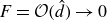 $F=\mathcal{O}(\hat {d})\to 0$
. Now, we introduce a stream function,
$F=\mathcal{O}(\hat {d})\to 0$
. Now, we introduce a stream function,
 $\varPsi$
,
$\varPsi$
,
 \begin{gather} \tilde {u}=\frac {d_0}{d}\partial _{\eta }\varPsi ,\quad \tilde {v}=-\partial _{\xi }\varPsi , \end{gather}
and its linearly perturbed form,
 \begin{align} \varPsi =\varPsi _0+\check {\varPsi }=\varPsi _0+\psi (\eta )\exp \left \{i\left (k\xi -t\left (\omega +k V_{\textit{ray}}\right )\right )\right \}\!, \end{align}
which implies
 \begin{align}&\quad\,\, \tilde {u}_0=\partial _{\eta }\varPsi _0,\quad \tilde {v}_0=-\partial _{\xi }\varPsi _0, \end{align}
 \begin{align}& \check {u}=\partial _{\eta }\check {\varPsi }-\frac {\hat {d}}{d_0}\partial _{\eta }\varPsi _0,\quad \check {v}=-\partial _{\xi }\check {\varPsi }. \end{align}
It is straightforward to show that
 $\varPsi$
according to (3.19) automatically satisfies the linearised non-dimensional form of the continuity (3.11a
) in curvilinear coordinates,
$\varPsi$
according to (3.19) automatically satisfies the linearised non-dimensional form of the continuity (3.11a
) in curvilinear coordinates,
 \begin{gather} \frac {\partial _\xi \hat {d}}{d_0}\tilde {u}_0+\partial _\xi \tilde {u}_0+\partial _\xi \check {u}+\partial _\eta \check {v}-\frac {\hat {d}}{d_0}\partial _\eta \tilde {v}_0=0. \end{gather}
Thus, we may write our linear stability problem in terms of
 $\varPsi$
(3.18) rather than
$\varPsi$
(3.18) rather than
 $\tilde {u}$
and
$\tilde {u}$
and
 $\tilde {v}$
.
$\tilde {v}$
.
Upon linearisation, we obtain the linearised curvilinear RANS equations in
 $\xi$
-direction,
$\xi$
-direction,
 \begin{align} &\mathrm{OS}_\xi : {{\textit{Re}}_{{G}}}\,ik\!\left \{\psi ^{\prime} \varPsi _0^{\prime} -\frac {\hat {d}}{d_0}\varPsi _0^{\prime 2}-\psi \varPsi _0^{\prime \prime} \right \}\!+{{\textit{Re}}_{{G}}}\,\tilde {l}_{\mathrm{t}}\left |\varPsi _0^{\prime \prime} \right |\!\left \{\tilde {l}_{\mathrm{t}}^{\prime}\!\left [\! k^2\!\left (\!-2\psi +3\frac {\hat {d}}{d_0}\eta \varPsi _0^{\prime}\!\right )\!-4\psi^{\prime \prime} \right .\right . \nonumber \\ &\quad\left .+\,6\frac {\hat {d}}{d_0}\varPsi _0^{\prime \prime} \right ]+\tilde {l}_{\mathrm{t}}\left [-2\psi ^{\prime \prime \prime} +6\frac {\hat {d}}{d_0}\varPsi _0^{\prime \prime \prime} -2\frac {\varPsi _0^{\prime \prime \prime} }{\varPsi _0^{\prime \prime} }\psi^{\prime \prime} +k^2\left (-{\psi}^{\prime}+\frac {3}{2}\frac {\hat {d}}{d_0}\varPsi _0^{\prime}+\frac {3}{2}\frac {\hat {d}}{d_0}\eta \varPsi _0^{\prime \prime} \right .\right . \nonumber \\ &\quad \left .\left .\left .-\,\frac {\varPsi _0^{\prime \prime \prime} }{\varPsi _0^{\prime \prime} }\psi +\frac {3}{2}\frac {\hat {d}}{d_0}\eta \frac {\varPsi _0^{\prime \prime \prime} \varPsi _0^{\prime} }{\varPsi _0^{\prime \prime} }\right )\right ]\right \}=-i k \hat {p}_{{G}}+\psi^{\prime \prime \prime} -3\frac {\hat {d}}{d_0}\varPsi _0^{\prime \prime \prime} \nonumber\\&\quad -k^2\left \{\psi^{\prime} -\frac {\hat {d}}{d_0}\varPsi _0^{\prime} -\frac {\hat {d}}{d_0}\eta {\varPsi _0^{\prime \prime}} \right \}\!, \end{align}
and in
 $\eta$
direction,
$\eta$
direction,
 \begin{align} &\mathrm{OS}_\eta : {{\textit{Re}}_{{G}}}\,k^2\left \{\psi \varPsi _0^{\prime} -\frac {\hat {d}}{d_0}\eta \varPsi _0^{\prime 2}\right \}+{{\textit{Re}}_{{G}}}\,\tilde {l}_{\mathrm{t}}\,\left |\varPsi _0^{\prime \prime} \right |ik\left \{2\tilde {l}_{\mathrm{t}}'\frac {\hat {d}}{d_0}\eta \varPsi _0^{\prime \prime} +\tilde {l}_{\mathrm{t}}\left [-2\psi ^{\prime \prime}+2\frac {\hat {d}}{d_0}\varPsi _0^{\prime \prime} \right .\right . \nonumber \\ &\quad\left .\left .+\, 2\eta \frac {\hat {d}}{d_0}\varPsi _0^{\prime \prime \prime} +k^2\left (-\psi +\frac {3}{2}\frac {\hat {d}}{d_0}\eta \varPsi _0^{\prime} \right )\right ]\right \}=-\hat {p}'_{{G}}-ik^3\left \{-\psi +\frac {\hat {d}}{d_0}\eta \varPsi _0^{\prime}\right \} \nonumber \\ &\quad -ik\left \{\psi^{\prime \prime} -2\frac {\hat {d}}{d_0}\varPsi _0^{\prime \prime} -\frac {\hat {d}}{d_0}\eta \varPsi _0^{\prime \prime \prime} \right \}\!, \end{align}
where primes denote differentiation with respect to
 $\eta$
. The pressure perturbation amplitude,
$\eta$
. The pressure perturbation amplitude,
 $\hat {p}_{{G}}$
, can be eliminated from (3.21a
) and (3.21b
) via the operation,
$\hat {p}_{{G}}$
, can be eliminated from (3.21a
) and (3.21b
) via the operation,
 \begin{align} \mathrm{OS}:\quad \partial _{\eta }\mathrm{OS}_\xi -ik\mathrm{OS}_\eta , \end{align}
yielding the final gas-side Orr–Sommerfeld equation, OS, which involves only
 $\psi$
and its derivatives. The problem is closed with the boundary conditions,
$\psi$
and its derivatives. The problem is closed with the boundary conditions,
 \begin{align} \left .{{\psi}^{\prime \prime}}\right |_{\eta =0}=0,\quad \left .{\psi }\right |_{\eta =0}=0,\quad \left .{{\psi}^{\prime}}\right |_{\eta =d_0}=0,\quad \left .{\psi }\right |_{\eta =d_0}=0. \end{align}
Finally, recasting (3.12) in the curvilinear coordinates (3.13), and perturbing and linearising around the primary flow, using (3.17) and (3.19), yields the perturbation amplitudes,
 $\hat {T}_{{G}}$
and
$\hat {T}_{{G}}$
and
 $\hat {P}_{{G}}$
,
$\hat {P}_{{G}}$
,
 \begin{align} \hat {T}_{{G}}&=-\left .{{\psi}^{\prime \prime}}\right |_{\eta =d_0}+2\frac {\hat {d}}{d_0}\left .{\varPsi _0^{\prime \prime}}\right |_{\eta =d_0},\nonumber \\ ik\hat {P}_{{G}}&=\left \{\left .{{\psi}^{\prime \prime \prime}}\right |_{\eta =d_0}-3\frac {\hat {d}}{d_0}\left .{\varPsi _0^{\prime \prime \prime}}\right |_{\eta =d_0}+k^2\hat {d}\,\left .{\varPsi _0^{\prime \prime}}\right |_{\eta =d_0}\right \}\!, \end{align}
for the perturbed interfacial gas stresses,
 \begin{align}&\qquad\qquad\qquad\qquad {T}_{{G}}=T_{{{G}} 0}+\check {T}_{{G}},\quad {P}_{{G}}={P}_{{{G}} 0}+\check {P}_{{G}}, \end{align}
 \begin{align}& \check {T}_{{G}}=\hat {T}_{{G}}\exp \left \{i\left (k\xi -t\left (\omega +k V_{\textit{ray}}\right )\right )\right \}\!,\quad \check {P}_{{G}}=\hat {P}_{{G}}\exp \left \{i\left (k\xi -t\left (\omega +k V_{\textit{ray}}\right )\right )\right \}\!, \end{align}
where we have again exploited that
 $x$
and
$x$
and
 $\xi$
collapse in the linear limit,
$\xi$
collapse in the linear limit,
 $\hat {d}\to 0$
, and, thus,
$\hat {d}\to 0$
, and, thus,
 $\partial _x\check {P}_{{G}}$
=
$\partial _x\check {P}_{{G}}$
=
 $\partial _\xi \check {P}_{{G}}$
.
$\partial _\xi \check {P}_{{G}}$
.
3.3.
Differentiated OS problem for the group velocity
 ${\rm d}\omega$
/
${\rm d}k$
${\rm d}\omega$
/
${\rm d}k$


In spatio-temporal linear stability analysis (Huerre & Monkewitz Reference Huerre and Monkewitz1990; Brevdo et al. Reference Brevdo, Laure, Dias and Bridges1999), instability is assessed by evaluating the temporal growth rate,
 $\omega _i$
, of perturbations that are fixed in the reference frame moving with the ray velocity,
$\omega _i$
, of perturbations that are fixed in the reference frame moving with the ray velocity,
 $V_{\textit{ray}}$
. The perturbations which remain at long time can be identified by setting the moving-frame group velocity,
$V_{\textit{ray}}$
. The perturbations which remain at long time can be identified by setting the moving-frame group velocity,
 ${\rm d}\omega$
/
${\rm d}\omega$
/
 ${\rm d}k\in \mathbb{C}$
, to zero, i.e.
${\rm d}k\in \mathbb{C}$
, to zero, i.e.
 ${\rm d}\omega$
/
${\rm d}\omega$
/
 ${\rm d}k$
= 0. In other words, the analysis checks whether perturbations that are fixed in the reference frame of a moving observer (in terms of the energy they carry) are seen to grow or to decay by that observer. In the case of convective instability (CI), the range of ray velocities
${\rm d}k$
= 0. In other words, the analysis checks whether perturbations that are fixed in the reference frame of a moving observer (in terms of the energy they carry) are seen to grow or to decay by that observer. In the case of convective instability (CI), the range of ray velocities
 $V_{\textit{ray}} \in [V_{\textit{ray}}^L, V_{\textit{ray}}^R]$
for which growing perturbations at long time are observed (
$V_{\textit{ray}} \in [V_{\textit{ray}}^L, V_{\textit{ray}}^R]$
for which growing perturbations at long time are observed (
 $\omega _i\gt 0$
and
$\omega _i\gt 0$
and
 ${\rm d}\omega$
/
${\rm d}\omega$
/
 ${\rm d}k=0$
) does not include the reference frame
${\rm d}k=0$
) does not include the reference frame
 $V_{\textit{ray}}=0$
. The upward-convective (respectively downward-convective) case corresponds to
$V_{\textit{ray}}=0$
. The upward-convective (respectively downward-convective) case corresponds to
 $V_{\textit{ray}}^L \lt V_{\textit{ray}}^R\lt 0$
(
$V_{\textit{ray}}^L \lt V_{\textit{ray}}^R\lt 0$
(
 $0 \lt V_{\textit{ray}}^L \lt V_{\textit{ray}}^R$
). In the case of AI, we have
$0 \lt V_{\textit{ray}}^L \lt V_{\textit{ray}}^R$
). In the case of AI, we have
 $\omega _i\gt 0$
at
$\omega _i\gt 0$
at
 ${\rm d}\omega$
/
${\rm d}\omega$
/
 ${\rm d}k$
= 0 and
${\rm d}k$
= 0 and
 $V_{\textit{ray}}=0$
.
$V_{\textit{ray}}=0$
.
To perform this analysis, a relation for the group velocity,
 ${\rm d}\omega$
/
${\rm d}\omega$
/
 ${\rm d}k$
, is required. We obtain this by differentiating the liquid side (3.7) and gas-side (3.21) OS eigenvalue problems with respect to the complex wave number,
${\rm d}k$
, is required. We obtain this by differentiating the liquid side (3.7) and gas-side (3.21) OS eigenvalue problems with respect to the complex wave number,
 $k$
. Thereby, we assume
$k$
. Thereby, we assume
 \begin{equation} \omega =\omega \left (k\right )\!,\quad c=c\left (k\right )\!,\quad \phi =\phi \left (k\right )\!,\quad \psi =\psi \left (k\right )\!, \end{equation}
and, for ease of notation, we will denote derivatives with respect to
 $k$
with a subscript
$k$
with a subscript
 $k$
,
$k$
,
 \begin{equation} \omega _k=\frac {{\rm d}\omega }{{\rm d}k},\quad c_k=\frac {{\rm d}c}{{\rm d}k},\quad \phi _k=\frac {{\rm d}\phi }{{\rm d}k},\quad \psi _k=\frac {{\rm d}\psi }{{\rm d}k}. \end{equation}
Differentiation of the liquid-side OS problem (3.7) with respect to
 $k$
yields the differentiated liquid-side OS equation,
$k$
yields the differentiated liquid-side OS equation,
 \begin{align} &\phi _k^{iv}-2k^2\phi _k^{\prime \prime}+k^4\phi _k-4k{\phi}^{\prime \prime}+4k^3\phi =i{\textit{Re}}_{{L}}\left \{\left (c+V_{\textit{ray}}-u_{{{L}} 0}\right )\left (k^2\phi -{\phi}^{\prime \prime}\right )-\phi u''_{{{L}} 0}\right \}\nonumber \\ &\quad +ik{\textit{Re}}_{{L}}\left \{c_k\left (k^2\phi -{\phi}^{\prime \prime}\right )+\left (c+V_{\textit{ray}}-u_{{{L}} 0}\right )\left (k^2\phi _k+2k\phi -\phi _k^{\prime \prime}\right )-\phi _k u''_{{{L}} 0}\right \}\!, \end{align}
the differentiated boundary conditions at
 $y$
= 0,
$y$
= 0,
 \begin{align} \phi _k^{\prime \prime}=\phi _k=0, \end{align}
and the differentiated inter-phase coupling conditions at
 $y$
=
$y$
=
 $h_0$
,
$h_0$
,
 \begin{align} &\phi _k\,u^{\prime\prime}_{{{L}} 0}+c_k\left \{{\phi}^{\prime \prime}+k^2\phi \right \}+\tilde {c}\left \{\phi _k^{\prime \prime}+2k\phi +k^2\phi _k\right \}=-\varPi _\mu \varPi _u\left \{\phi _k\frac {\hat {T}_{{G}}}{\hat {d}}+\phi \frac {\rm d}{{\rm d}k}\left (\frac {\hat {T}_{{G}}}{\hat {d}}\right )\right \}\!, \end{align}
 \begin{align} &-\frac {1}{{\textit{Re}}_{{L}}}\left \{4k\phi u^{\prime}_{{{L}} 0}+2k^2\phi _k u_{{{L}} 0}'+c_k\left [3 k^2{\phi}^{\prime}-{\phi}^{\prime \prime \prime}\right ]+\tilde {c}\left [6 k{\phi}^{\prime}+3 k^2{\phi}^{\prime}_k-\phi _k^{\prime \prime \prime}\right ]\right \}\nonumber \\ &-i \tilde {c}\left \{-\tilde {c}\,{\phi}^{\prime}-\phi \,u_{{{L}} 0}\right \}-i k\,c_k\left \{-\tilde {c}\,{\phi}^{\prime}-\phi \,u_{{{L}} 0}\right \}-i k\,\tilde {c}\left \{-c_k\,{\phi}^{\prime}-\tilde {c}\,\phi _k^{\prime}-\phi _k\,u_{{{L}} 0}\right \} \nonumber \\ &+i\phi p^{\prime}_{{{L}} 0}+ik\phi^{\prime} _k p_{{{L}} 0}=\frac {\varPi _\rho \varPi _u^2}{{{\textit{Re}}_{{G}}}}\left \{\phi _k ik\frac {\hat {P}_{{G}}}{\hat {d}}+\phi \frac {\rm d}{{\rm d}k}\left (ik\frac {\hat {P}_{{G}}}{\hat {d}}\right )\right \}+i{\textit{We}}\,\left (3k^2\phi + k^3\phi _k\right ). \end{align}
Differentiation of the gas-side OS problem (3.21) with respect to
 $k$
yields the differentiated form of the gas-side OS (3.21c
),
$k$
yields the differentiated form of the gas-side OS (3.21c
),
 \begin{align} \mathrm{OS}_k\equiv \frac {\mathrm{d OS}}{\mathrm{d}k}, \end{align}
and the differentiated boundary conditions,
 \begin{align} \left .{\psi _k^{\prime \prime}}\right |_{\eta =0}=0,\quad \left .{\psi _k}\right |_{\eta =0}=0,\quad \left .{\psi _k^{\prime}}\right |_{\eta =d_0}=0,\quad \left .{\psi _k}\right |_{\eta =d_0}=0. \end{align}
Finally, differentiation of (3.22) with respect to
 $k$
, yields the differentiated interfacial gas stress amplitudes,
$k$
, yields the differentiated interfacial gas stress amplitudes,
 \begin{gather} \frac {\rm d}{{\rm d}k}\left (\frac {\hat {T}_{{G}}}{\hat {d}}\right )=-\frac {\left .{{\psi}^{\prime \prime}_k}\right |_{\eta =d_0}}{\hat {d}},\quad \frac {\rm d}{{\rm d}k}\left (ik\frac {\hat {P}_{{G}}}{\hat {d}}\right )=\frac {\left .{{\psi}^{\prime \prime \prime}_k}\right |_{\eta =d_0}}{\hat {d}}+2k\left .{\varPsi _0^{\prime \prime}}\right |_{\eta =d_0}, \end{gather}
where we have exploited that
 $\hat {d}$
is independent of
$\hat {d}$
is independent of
 $k$
. The eigenvalue problem given by (3.26) and (3.27) can then be solved for the group velocity,
$k$
. The eigenvalue problem given by (3.26) and (3.27) can then be solved for the group velocity,
 $\omega _k$
, which enters through the differentiated form of (3.6),
$\omega _k$
, which enters through the differentiated form of (3.6),
 \begin{equation} c_k=\frac {\omega _k}{k}-\frac {c}{k}. \end{equation}
3.4. Numerical methods and code validation
Equations (3.7) and (3.21) constitute an eigenvalue problem (EVP) for the complex wave speed,
 $c$
=
$c$
=
 $\omega$
/
$\omega$
/
 $k$
, and (3.26) and (3.27) constitute an EVP for the complex group velocity,
$k$
, and (3.26) and (3.27) constitute an EVP for the complex group velocity,
 $\omega _k$
. In addition to the main control parameters, e.g.
$\omega _k$
. In addition to the main control parameters, e.g.
 ${\textit{Re}}_{{L}}$
,
${\textit{Re}}_{{L}}$
,
 ${\textit{Re}}_{{G}}$
,
${\textit{Re}}_{{G}}$
,
 $\beta$
,
$\beta$
,
 ${\textit{Ka}}$
and
${\textit{Ka}}$
and
 $H^\star$
, this system contains seven variables, i.e.
$H^\star$
, this system contains seven variables, i.e.
 $\omega _r$
,
$\omega _r$
,
 $\omega _i$
,
$\omega _i$
,
 $k_r$
,
$k_r$
,
 $k_i$
,
$k_i$
,
 ${\rm Re} \{\omega _k\}$
,
${\rm Re} \{\omega _k\}$
,
 ${\rm Im} \{\omega _k\}$
and
${\rm Im} \{\omega _k\}$
and
 $V_{\textit{ray}}$
. Each EVP imposes one complex constraint, i.e. two equations involving these variables. Thus, there are four constraints in total, which means that three variables need to be fixed in each type of stability calculation.
$V_{\textit{ray}}$
. Each EVP imposes one complex constraint, i.e. two equations involving these variables. Thus, there are four constraints in total, which means that three variables need to be fixed in each type of stability calculation.
In a spatial formulation, we will fix
 $\omega _i$
=
$\omega _i$
=
 $V_{\textit{ray}}$
= 0 and vary
$V_{\textit{ray}}$
= 0 and vary
 $\omega _r$
with the goal of obtaining the spatial growth rate,
$\omega _r$
with the goal of obtaining the spatial growth rate,
 $k_i$
(e.g. figure 8
b). In a temporal formulation, we will fix
$k_i$
(e.g. figure 8
b). In a temporal formulation, we will fix
 $k_i$
=
$k_i$
=
 $V_{\textit{ray}}$
= 0 and vary
$V_{\textit{ray}}$
= 0 and vary
 $k_r$
with the goal of obtaining
$k_r$
with the goal of obtaining
 $\omega _i$
(e.g. figure 10
a). In both these calculations, the group velocity,
$\omega _i$
(e.g. figure 10
a). In both these calculations, the group velocity,
 $\omega _k$
, is auxiliary. By contrast, in a spatio-temporal formulation, we will fix
$\omega _k$
, is auxiliary. By contrast, in a spatio-temporal formulation, we will fix
 ${\rm Re} \{\omega _k\}$
=
${\rm Re} \{\omega _k\}$
=
 ${\rm Im} \{\omega _k\}$
= 0 and vary
${\rm Im} \{\omega _k\}$
= 0 and vary
 $V_{\textit{ray}}$
with the goal of obtaining the temporal growth rate,
$V_{\textit{ray}}$
with the goal of obtaining the temporal growth rate,
 $\omega _i$
, of the perturbation that remains at long time in the reference frame moving with
$\omega _i$
, of the perturbation that remains at long time in the reference frame moving with
 $V_{\textit{ray}}$
(e.g. figure 11).
$V_{\textit{ray}}$
(e.g. figure 11).
In all cases, we will solve the combined eigenvalue problem via numerical continuation, using the software Auto07P (Doedel & Oldeman Reference Doedel and Oldeman2009). This is made possible by the existence of an analytical solution for the Kapitza instability mode, from which to start the continuation. This analytical solution is readily obtained by assuming a laminar gas flow (
 $\tilde {l}_t$
= 0), and by considering the long-wave limit,
$\tilde {l}_t$
= 0), and by considering the long-wave limit,
 $k_r$
= 0, where
$k_r$
= 0, where
 $k_i$
=
$k_i$
=
 $\omega _i$
=
$\omega _i$
=
 ${\rm Im} \{\omega _k\}$
= 0, and
${\rm Im} \{\omega _k\}$
= 0, and
 $\omega _r$
and
$\omega _r$
and
 ${\rm Re} \{\omega _k\}$
are known functions of the control parameters, and where we can set
${\rm Re} \{\omega _k\}$
are known functions of the control parameters, and where we can set
 $V_{\textit{ray}}$
= 0 without loss of generality. No such analytical solution exists for the new ISW mode. However, the ISW mode merges with the Kapitza mode at large values of
$V_{\textit{ray}}$
= 0 without loss of generality. No such analytical solution exists for the new ISW mode. However, the ISW mode merges with the Kapitza mode at large values of
 $|{{\textit{Re}}_{{G}}}|$
, and the merged mode always originates at
$|{{\textit{Re}}_{{G}}}|$
, and the merged mode always originates at
 $k_r$
=
$k_r$
=
 $k_i$
=
$k_i$
=
 $\omega _i$
=
$\omega _i$
=
 ${\rm Im} \{\omega _k\}$
= 0. Thus, by moving onto the relevant portion of the merged mode and by subsequently reducing
${\rm Im} \{\omega _k\}$
= 0. Thus, by moving onto the relevant portion of the merged mode and by subsequently reducing
 $|{{\textit{Re}}_{{G}}}|$
, the ISW mode can be captured. In conclusion, a continuation path with origin at
$|{{\textit{Re}}_{{G}}}|$
, the ISW mode can be captured. In conclusion, a continuation path with origin at
 $k_r$
= 0 can be constructed both for the Kapitza instability mode and for the ISW mode.
$k_r$
= 0 can be constructed both for the Kapitza instability mode and for the ISW mode.
In the latter part of this subsection, we will validate our numerical procedure by reproducing several results from the literature (Brevdo et al. Reference Brevdo, Laure, Dias and Bridges1999; Vellingiri et al. Reference Vellingiri, Tseluiko and Kalliadasis2015; Schmidt et al. Reference Schmidt, Náraigh, Lucquiaud and Valluri2016). Before that, we outline the continuation sequence that we have applied for obtaining physical saddle points (SPs) in the context of our spatio-temporal stability calculations. By physical SPs, we mean saddle points that satisfy the Briggs collision criterion (Briggs Reference Briggs1964).
The first step of this sequence is to perform a temporal stability calculation (
 $k_i$
=
$k_i$
=
 $V_{\textit{ray}}$
= 0), where we continue
$V_{\textit{ray}}$
= 0), where we continue
 $k_r$
until reaching the maximum of the dispersion curve for
$k_r$
until reaching the maximum of the dispersion curve for
 $\omega _i$
, where
$\omega _i$
, where
 ${\rm Im} \{\omega _k\}$
= 0. Next, we fix
${\rm Im} \{\omega _k\}$
= 0. Next, we fix
 ${\rm Im} \{\omega _k\}$
=
${\rm Im} \{\omega _k\}$
=
 $V_{\textit{ray}}$
= 0 and continue
$V_{\textit{ray}}$
= 0 and continue
 ${\rm Re} \{\omega _k\}$
, until reaching
${\rm Re} \{\omega _k\}$
, until reaching
 ${\rm Re} \{\omega _k\}$
= 0. Finally, we fix
${\rm Re} \{\omega _k\}$
= 0. Finally, we fix
 ${\rm Re} \{\omega _k\}$
=
${\rm Re} \{\omega _k\}$
=
 ${\rm Im} \{\omega _k\}$
= 0 and continue
${\rm Im} \{\omega _k\}$
= 0 and continue
 $V_{\textit{ray}}$
across the desired range, thus obtaining the SP curve in terms of
$V_{\textit{ray}}$
across the desired range, thus obtaining the SP curve in terms of
 $\omega _i$
versus
$\omega _i$
versus
 $V_{\textit{ray}}$
(see e.g. figure 7
a). To check whether the Briggs collision criterion is satisfied at a given SP, we check how the colliding spatial branches, i.e. curves of constant
$V_{\textit{ray}}$
(see e.g. figure 7
a). To check whether the Briggs collision criterion is satisfied at a given SP, we check how the colliding spatial branches, i.e. curves of constant
 $\omega _i$
and fixed
$\omega _i$
and fixed
 $V_{\textit{ray}}$
in the
$V_{\textit{ray}}$
in the
 $k_r$
–
$k_r$
–
 $k_i$
plane, move away from the SP as
$k_i$
plane, move away from the SP as
 $\omega _i$
is increased from
$\omega _i$
is increased from
 $\omega _i$
=
$\omega _i$
=
 $\omega _i^{\textit{SP}}$
to beyond the maximum temporal growth rate,
$\omega _i^{\textit{SP}}$
to beyond the maximum temporal growth rate,
 $\omega _i^{\textit{max}}$
, obtained from the temporal stability formulation. Depending on how the spatial branches evolve during this process, they can best be tracked either by fixing
$\omega _i^{\textit{max}}$
, obtained from the temporal stability formulation. Depending on how the spatial branches evolve during this process, they can best be tracked either by fixing
 ${\rm Im} \{\omega _k\}$
= 0 (extremum of a spatial branch),
${\rm Im} \{\omega _k\}$
= 0 (extremum of a spatial branch),
 ${\rm Re} \{\omega _k\}$
= 0 (limit point of a spatial branch),
${\rm Re} \{\omega _k\}$
= 0 (limit point of a spatial branch),
 $k_r$
or
$k_r$
or
 $k_i$
. An SP is physical, if, in the
$k_i$
. An SP is physical, if, in the
 $k_r$
–
$k_r$
–
 $k_i$
plane, a continuous integration path that remains between the two spatial branches without intersecting these for all
$k_i$
plane, a continuous integration path that remains between the two spatial branches without intersecting these for all
 $\omega _i\gt \omega _i^{\textit{SP}}$
can be constructed by simple deformation and/or translation of the initial path,
$\omega _i\gt \omega _i^{\textit{SP}}$
can be constructed by simple deformation and/or translation of the initial path,
 $k_i$
= 0, at
$k_i$
= 0, at
 $\omega _i$
=
$\omega _i$
=
 $\omega _i^{\textit{max}}$
(Briggs Reference Briggs1964).
$\omega _i^{\textit{max}}$
(Briggs Reference Briggs1964).
Spatio-temporal linear stability calculations for the conditions in figure 4(a) of Brevdo et al. (Reference Brevdo, Laure, Dias and Bridges1999). Inclined falling liquid film in a passive atmosphere:
 ${\textit{Ka}}$
= 331.85,
${\textit{Ka}}$
= 331.85,
 $\beta ={4.6}^\circ$
,
$\beta ={4.6}^\circ$
,
 $\varPi _\rho$
=
$\varPi _\rho$
=
 $\varPi _\mu$
= 0. (a) Saddle point (SP) curves. Upward triangles,
$\varPi _\mu$
= 0. (a) Saddle point (SP) curves. Upward triangles,
 $R$
=
$R$
=
 $(3/2){\textit{Re}}_{{L}}$
= 20; downward triangles,
$(3/2){\textit{Re}}_{{L}}$
= 20; downward triangles,
 $R$
= 40; squares,
$R$
= 40; squares,
 $R$
= 60; diamonds,
$R$
= 60; diamonds,
 $R$
= 100; circles (branch I) and crosses (branch II),
$R$
= 100; circles (branch I) and crosses (branch II),
 $R$
= 200. Dotted line segments correspond to unphysical SPs. (b–d) Collisions of spatial branches at the SPs marked by large coloured symbols in panel (a),
$R$
= 200. Dotted line segments correspond to unphysical SPs. (b–d) Collisions of spatial branches at the SPs marked by large coloured symbols in panel (a),
 $R$
= 200. Solid and dashed spatial branches move toward the corresponding SP as
$R$
= 200. Solid and dashed spatial branches move toward the corresponding SP as
 $\omega _i$
is decreased. (b)
$\omega _i$
is decreased. (b)
 $V^\star _{\textit{ray}}/\mathcal{U}_{{Nu}}$
= 1.16, branch II: unphysical collision,
$V^\star _{\textit{ray}}/\mathcal{U}_{{Nu}}$
= 1.16, branch II: unphysical collision,
 $\omega ^\star _i\mathcal{T}_{{Nu}}$
= [0.02, 0.015, 0.01, 0.0079]; (c)
$\omega ^\star _i\mathcal{T}_{{Nu}}$
= [0.02, 0.015, 0.01, 0.0079]; (c)
 $V^\star _{\textit{ray}}/\mathcal{U}_{{Nu}}$
= 1.16, branch I: physical collision,
$V^\star _{\textit{ray}}/\mathcal{U}_{{Nu}}$
= 1.16, branch I: physical collision,
 $\omega ^\star _i\mathcal{T}_{{Nu}}$
= [0.02, 0.015, 0.01, 0.0079, 0.0076]. Red dash-dotted line:
$\omega ^\star _i\mathcal{T}_{{Nu}}$
= [0.02, 0.015, 0.01, 0.0079, 0.0076]. Red dash-dotted line:
 ${\rm Im} \{\omega _k\}$
= 0; (d)
${\rm Im} \{\omega _k\}$
= 0; (d)
 $V^\star _{\textit{ray}}/\mathcal{U}_{{Nu}}$
= 1.23,
$V^\star _{\textit{ray}}/\mathcal{U}_{{Nu}}$
= 1.23,
 $\omega ^\star _i\mathcal{T}_{{Nu}}$
= [0.0151, 0.0149, 0.0148, 0.014, 0.013, 0.0121]. Open circle, branch I, physical collision; cross, branch II, unphysical collision. Black solid and dotted lines, SP curves from panel (a).
$\omega ^\star _i\mathcal{T}_{{Nu}}$
= [0.0151, 0.0149, 0.0148, 0.014, 0.013, 0.0121]. Open circle, branch I, physical collision; cross, branch II, unphysical collision. Black solid and dotted lines, SP curves from panel (a).

To validate our numerical procedure outlined previously, we started by reproducing the spatio-temporal stability calculations in figure 4(a) of Brevdo et al. (Reference Brevdo, Laure, Dias and Bridges1999), where a falling liquid film flowing in a passive atmosphere was considered. Results of our calculations are represented in figure 7. The SP curves in figure 7(a) are in excellent agreement with figure 4(a) of Brevdo et al. (Reference Brevdo, Laure, Dias and Bridges1999). To facilitate comparison with the reference, we have rescaled our results with the Nusselt scales (subscript Nu), named after the work of Nusselt (Reference Nusselt1916):
 \begin{gather} \mathcal{L}_{{Nu}}=\lim _{\varPi _\rho ,\varPi _\mu \to 0}\left \{h^\star _0\right \}\!,\quad \mathcal{U}_{{Nu}}=\lim _{\varPi _\rho ,\varPi _\mu \to 0}\left \{u^\star _{{{L}} 0}|_{y=h_0}\right \}\!,\quad \mathcal{T}_{{Nu}}=\frac {\mathcal{L}_{{Nu}}}{\mathcal{U}_{{Nu}}}. \end{gather}
For the largest value of the modified liquid Reynolds number,
 $R$
=
$R$
=
 $(3/2){{\textit{Re}}_{{L}}}$
, in figure 7(a), i.e.
$(3/2){{\textit{Re}}_{{L}}}$
, in figure 7(a), i.e.
 $R$
= 200, two SP curves are obtained. However, as a consequence of the Briggs collision criterion, there can be only one physical SP for every value of
$R$
= 200, two SP curves are obtained. However, as a consequence of the Briggs collision criterion, there can be only one physical SP for every value of
 $V_{\textit{ray}}$
. The dotted portion of branch II demarcates unphysical SPs, as identified by our own calculations of the collision of spatial branches, examples of which are represented in figures 7(b) (unphysical collision, branch II), 7(c) (physical collision, branch I) and 7(d) (physical collision for branch I and unphysical collision for branch II), for the SPs marked by large coloured symbols in figure 7(a). Compared with Brevdo et al. (Reference Brevdo, Laure, Dias and Bridges1999), the unphysical segment of branch II is significantly longer. This is because we consider collisions of the type shown in figure 7(b) as unphysical, as the spatial branches intersect before colliding at the SP.
$V_{\textit{ray}}$
. The dotted portion of branch II demarcates unphysical SPs, as identified by our own calculations of the collision of spatial branches, examples of which are represented in figures 7(b) (unphysical collision, branch II), 7(c) (physical collision, branch I) and 7(d) (physical collision for branch I and unphysical collision for branch II), for the SPs marked by large coloured symbols in figure 7(a). Compared with Brevdo et al. (Reference Brevdo, Laure, Dias and Bridges1999), the unphysical segment of branch II is significantly longer. This is because we consider collisions of the type shown in figure 7(b) as unphysical, as the spatial branches intersect before colliding at the SP.
Linear stability calculations for gas-sheared vertically falling liquid films. (a) Temporal calculations for the conditions in figure 4(e) of Schmidt et al. (Reference Schmidt, Náraigh, Lucquiaud and Valluri2016):
 $H^\star ={10}\,\textrm {mm}$
,
$H^\star ={10}\,\textrm {mm}$
,
 ${\textit{Ka}}$
= 117.71,
${\textit{Ka}}$
= 117.71,
 ${{\textit{Re}}_{{L}}}=6166$
,
${{\textit{Re}}_{{L}}}=6166$
,
 ${\textit{Re}}_{{G}}$
= –48 322,
${\textit{Re}}_{{G}}$
= –48 322,
 $\delta _{{L}}$
=
$\delta _{{L}}$
=
 $h_0$
=
$h_0$
=
 $h_0$
/
$h_0$
/
 $H^\star$
= 0.08,
$H^\star$
= 0.08,
 $\underline{Fr}= \underline{\mathcal{U}}/\sqrt {gH^\star }=3$
, where
$\underline{Fr}= \underline{\mathcal{U}}/\sqrt {gH^\star }=3$
, where
 $\underline{\mathcal{U}}$
=
$\underline{\mathcal{U}}$
=
 $[\partial _{x^\star }P_{{{G}} 0}^\star H^\star /\rho _{{G}}]^{1/2}$
. Solid, numerical continuation with Auto07P; crosses, Chebyshev collocation approach (Ishimura et al. Reference Ishimura, Mergui, Ruyer-Quil and Dietze2023). (b) Spatial calculations for the conditions in figure 16 of Vellingiri et al. (Reference Vellingiri, Tseluiko and Kalliadasis2015):
$[\partial _{x^\star }P_{{{G}} 0}^\star H^\star /\rho _{{G}}]^{1/2}$
. Solid, numerical continuation with Auto07P; crosses, Chebyshev collocation approach (Ishimura et al. Reference Ishimura, Mergui, Ruyer-Quil and Dietze2023). (b) Spatial calculations for the conditions in figure 16 of Vellingiri et al. (Reference Vellingiri, Tseluiko and Kalliadasis2015):
 $H^\star ={30}\,\textrm {mm}$
,
$H^\star ={30}\,\textrm {mm}$
,
 ${\textit{Ka}}=1988.5$
,
${\textit{Ka}}=1988.5$
,
 $\underline{Re}$
=
$\underline{Re}$
=
 $gh_0^{\star 3}$
/
$gh_0^{\star 3}$
/
 $\nu _{{L}}^2$
= 10,
$\nu _{{L}}^2$
= 10,
 $\varTheta \in [0.1,2.5]$
, with
$\varTheta \in [0.1,2.5]$
, with
 $\varTheta =T_{{G}}^\star /(\rho _{{L}} g^{2/3}\nu _{{L}}^{2/3})$
.
$\varTheta =T_{{G}}^\star /(\rho _{{L}} g^{2/3}\nu _{{L}}^{2/3})$
.

Next, we reproduced the temporal stability calculations in figure 4(e) of Schmidt et al. (Reference Schmidt, Náraigh, Lucquiaud and Valluri2016), where a vertically falling liquid film sheared by a confined counter-current laminar gas flow was considered. Results of our calculations (obtained in the laminar limit,
 $\tilde {l}_t$
= 0) are represented in figure 8(a). The data represented by a solid curve were obtained via our numerical continuation approach, whereas symbols mark results obtained with the Chebyshev collocation approach that was introduced by Ishimura et al. (Reference Ishimura, Mergui, Ruyer-Quil and Dietze2023) (using
$\tilde {l}_t$
= 0) are represented in figure 8(a). The data represented by a solid curve were obtained via our numerical continuation approach, whereas symbols mark results obtained with the Chebyshev collocation approach that was introduced by Ishimura et al. (Reference Ishimura, Mergui, Ruyer-Quil and Dietze2023) (using
 $N_{{p}}$
= 100 collocation points in each phase). Both data sets agree very well with the blue solid curve in figure 4(e) of Schmidt et al. (Reference Schmidt, Náraigh, Lucquiaud and Valluri2016), which corresponds to what was termed as interfacial mode in that reference. As stated in § 1, we will show that this gas-induced instability mode is related to the merged mode observed in our configuration.
$N_{{p}}$
= 100 collocation points in each phase). Both data sets agree very well with the blue solid curve in figure 4(e) of Schmidt et al. (Reference Schmidt, Náraigh, Lucquiaud and Valluri2016), which corresponds to what was termed as interfacial mode in that reference. As stated in § 1, we will show that this gas-induced instability mode is related to the merged mode observed in our configuration.
Finally, we have reproduced the spatial stability calculations in figure 16 of Vellingiri et al. (Reference Vellingiri, Tseluiko and Kalliadasis2015), where a vertically falling liquid film sheared by a confined counter-current turbulent gas flow was considered. Results of our calculations are represented in figure 8(b). These are in good agreement with the reference. In addition, we have performed spatio-temporal calculations for the same operating conditions as in figure 8(b). Results of these calculations are represented in figure 9. These allow to predict the evolution of linear perturbations within the AI gap, where the spatial calculations in figure 8(b) break down. In particular, figure 9(b) allows to determine the wave number associated with the fastest growing perturbations in this range, which is marked by filled symbols in figures 9(a) and 9(b).
Spatio-temporal stability calculations for the conditions in figure 8(b). SP curves (
 $\omega _k$
= 0) for selected values of
$\omega _k$
= 0) for selected values of
 $\varTheta$
. Circles,
$\varTheta$
. Circles,
 $\varTheta$
= 1.0; upward triangles,
$\varTheta$
= 1.0; upward triangles,
 $\varTheta$
= 1.21 (downward-CI/AI transition); diamonds,
$\varTheta$
= 1.21 (downward-CI/AI transition); diamonds,
 $\varTheta$
= 1.25; downward triangles,
$\varTheta$
= 1.25; downward triangles,
 $\varTheta$
= 1.91 (AI/upward-CI transition); squares,
$\varTheta$
= 1.91 (AI/upward-CI transition); squares,
 $\varTheta$
= 2.5. (a) Temporal growth rate of perturbations persisting at long time; (b) wave speed. Filled symbols mark maximum
$\varTheta$
= 2.5. (a) Temporal growth rate of perturbations persisting at long time; (b) wave speed. Filled symbols mark maximum
 $\omega _i$
.
$\omega _i$
.

Two of the SP curves plotted in figure 9(a) correspond to the downward-CI/AI transition (upward triangles,
 $\varTheta$
= 1.21) and to the AI/upward-CI transition (downward triangles,
$\varTheta$
= 1.21) and to the AI/upward-CI transition (downward triangles,
 $\varTheta$
= 1.91). The corresponding critical values of the dimensionless gas shear stress,
$\varTheta$
= 1.91). The corresponding critical values of the dimensionless gas shear stress,
 $\varTheta$
=
$\varTheta$
=
 $T_{{G}}^\star$
/
$T_{{G}}^\star$
/
 $(\rho _{{L}} g^{2/3}\nu _{{L}}^{2/3})$
, can be directly compared with the lower and upper limit of the AI gap reported in table 1 of Vellingiri et al. (Reference Vellingiri, Tseluiko and Kalliadasis2015). While the lower limit is in excellent agreement with our data, there is a 9 % error on the upper limit (
$(\rho _{{L}} g^{2/3}\nu _{{L}}^{2/3})$
, can be directly compared with the lower and upper limit of the AI gap reported in table 1 of Vellingiri et al. (Reference Vellingiri, Tseluiko and Kalliadasis2015). While the lower limit is in excellent agreement with our data, there is a 9 % error on the upper limit (
 $\varTheta$
= 1.91 versus
$\varTheta$
= 1.91 versus
 $\varTheta$
= 2.1 in the reference). After careful verification (see figures 23
a and 24 and their discussion in Appendices A and B), we believe that this can be attributed to having accounted for linear perturbations of turbulent stresses in our current work and to having used different curvilinear coordinates than Vellingiri et al. (Reference Vellingiri, Tseluiko and Kalliadasis2015).
$\varTheta$
= 2.1 in the reference). After careful verification (see figures 23
a and 24 and their discussion in Appendices A and B), we believe that this can be attributed to having accounted for linear perturbations of turbulent stresses in our current work and to having used different curvilinear coordinates than Vellingiri et al. (Reference Vellingiri, Tseluiko and Kalliadasis2015).
4. Results
In this section, we present the results of our linear stability calculations of gas-sheared falling liquids films, using the approach outlined in § 3, and compare these with our own experiments (see figure 21
b) discussed in § 2. We have performed calculations for different liquid/air combinations, properties of which are listed in table 1. Thereby, we have chosen representative real liquids spanning a wide range of the Kapitza number,
 ${\textit{Ka}}$
. Particular attention is paid to the water/air system, based on the fluid properties reported by Ishimura et al. (Reference Ishimura, Mergui, Ruyer-Quil and Dietze2023), to ensure comparison with that reference. However, whenever performing direct comparisons with our experiments (see figures 4
b and 21
b), we have used the corresponding fluid properties specified in § 2.
${\textit{Ka}}$
. Particular attention is paid to the water/air system, based on the fluid properties reported by Ishimura et al. (Reference Ishimura, Mergui, Ruyer-Quil and Dietze2023), to ensure comparison with that reference. However, whenever performing direct comparisons with our experiments (see figures 4
b and 21
b), we have used the corresponding fluid properties specified in § 2.
Fluid properties used in our computations. The Kapitza number is
 ${{\textit{Ka}}}=\sigma /\rho _{{L}}/g^{1/3}/\nu _{{L}}^{4/3}$
, where
${{\textit{Ka}}}=\sigma /\rho _{{L}}/g^{1/3}/\nu _{{L}}^{4/3}$
, where
 $g={9.81}\,\textrm {m}\,\textrm {s}^{-2}$
denotes the gravitational acceleration. Numbers between parentheses give the solvent mass fraction of aqueous solutions.
$g={9.81}\,\textrm {m}\,\textrm {s}^{-2}$
denotes the gravitational acceleration. Numbers between parentheses give the solvent mass fraction of aqueous solutions.

Temporal linear stability calculations. Parameters according to Ishimura et al. (Reference Ishimura, Mergui, Ruyer-Quil and Dietze2023): water/air (
 ${\textit{Ka}}$
= 3174),
${\textit{Ka}}$
= 3174),
 $\beta ={5}^\circ$
,
$\beta ={5}^\circ$
,
 $H^\star ={13}\,\textrm {mm}$
,
$H^\star ={13}\,\textrm {mm}$
,
 ${\textit{Re}}_{{L}}$
= 43.1. Thick solid blue with filled symbols, ISW mode; dashed black with open symbols, Kapitza mode; thin solid red with open symbols, unstable merged mode. Circles,
${\textit{Re}}_{{L}}$
= 43.1. Thick solid blue with filled symbols, ISW mode; dashed black with open symbols, Kapitza mode; thin solid red with open symbols, unstable merged mode. Circles,
 ${\textit{Re}}_{{G}}$
= –4700; squares,
${\textit{Re}}_{{G}}$
= –4700; squares,
 ${\textit{Re}}_{{G}}$
= –5200; diamonds,
${\textit{Re}}_{{G}}$
= –5200; diamonds,
 ${\textit{Re}}_{{G}}$
= –5750; pentagons,
${\textit{Re}}_{{G}}$
= –5750; pentagons,
 ${\textit{Re}}_{{G}}$
= –6620. (a) Growth rate,
${\textit{Re}}_{{G}}$
= –6620. (a) Growth rate,
 $\omega _i$
; (b) wave speed,
$\omega _i$
; (b) wave speed,
 $c_r$
=
$c_r$
=
 $\omega _r$
/
$\omega _r$
/
 $k_r$
.
$k_r$
.

4.1. Spatio-temporal characterisation of Kapitza, ISW and merged mode
In this subsection, we will characterise the spatio-temporal linear responses associated with the Kapitza, ISW and merged instability modes, via spatio-temporal linear stability calculations, following the continuation procedure outlined in § 3.4.
Before that, we discuss figure 10, where we have plotted results from temporal linear stability calculations for the conditions used by Ishimura et al. (Reference Ishimura, Mergui, Ruyer-Quil and Dietze2023), i.e. water/air (
 ${\textit{Ka}}$
= 3174),
${\textit{Ka}}$
= 3174),
 $\beta ={5}^\circ$
,
$\beta ={5}^\circ$
,
 $H^\star ={13}\,\textrm {mm}$
and
$H^\star ={13}\,\textrm {mm}$
and
 ${\textit{Re}}_{{L}}$
= 43.1. The figure represents dispersion curves of the temporal growth rate,
${\textit{Re}}_{{L}}$
= 43.1. The figure represents dispersion curves of the temporal growth rate,
 $\omega _i$
(figure 10
a), and wave speed,
$\omega _i$
(figure 10
a), and wave speed,
 $c_r$
(figure 10
b), versus the wave number,
$c_r$
(figure 10
b), versus the wave number,
 $k_r$
. These curves obtained by continuation agree well with the Chebyshev calculation of Ishimura et al. (Reference Ishimura, Mergui, Ruyer-Quil and Dietze2023). Different symbols correspond to different values of the gas Reynolds number,
$k_r$
. These curves obtained by continuation agree well with the Chebyshev calculation of Ishimura et al. (Reference Ishimura, Mergui, Ruyer-Quil and Dietze2023). Different symbols correspond to different values of the gas Reynolds number,
 ${\textit{Re}}_{{G}}$
. At low values of
${\textit{Re}}_{{G}}$
. At low values of
 $|{{\textit{Re}}_{{G}}}|$
, the Kapitza mode (dashed black curves with open symbols) and the ISW mode (solid blue curves with filled symbols) are separated and distinct. Upon increasing
$|{{\textit{Re}}_{{G}}}|$
, the Kapitza mode (dashed black curves with open symbols) and the ISW mode (solid blue curves with filled symbols) are separated and distinct. Upon increasing
 $|{{\textit{Re}}_{{G}}}|$
, the two modes coalesce to form an unstable merged mode (thin solid red curves with open diamonds and pentagons). This merged mode is concatenated from the short-wave portion of the ISW mode and the long-wave portion of the Kapitza mode (a second, stable, merged mode, not represented in figure 10, results from the coalescence of the remaining opposing portions). At
$|{{\textit{Re}}_{{G}}}|$
, the two modes coalesce to form an unstable merged mode (thin solid red curves with open diamonds and pentagons). This merged mode is concatenated from the short-wave portion of the ISW mode and the long-wave portion of the Kapitza mode (a second, stable, merged mode, not represented in figure 10, results from the coalescence of the remaining opposing portions). At
 ${\textit{Re}}_{{G}}$
= –5750 (diamonds), the merged mode displays two maxima that are comparable in magnitude. Then, at
${\textit{Re}}_{{G}}$
= –5750 (diamonds), the merged mode displays two maxima that are comparable in magnitude. Then, at
 ${\textit{Re}}_{{G}}$
= –6620 (pentagons), the short-wave maximum becomes dominant. As shown in figure 10(b), both the ISW mode and the merged mode are associated with negative values of the linear wave speed,
${\textit{Re}}_{{G}}$
= –6620 (pentagons), the short-wave maximum becomes dominant. As shown in figure 10(b), both the ISW mode and the merged mode are associated with negative values of the linear wave speed,
 $c_r$
.
$c_r$
.
SP curves obtained from spatio-temporal linear stability calculations. Parameters according to figure 10: water/air (
 ${\textit{Ka}}$
= 3174),
${\textit{Ka}}$
= 3174),
 $\beta ={5}^\circ$
,
$\beta ={5}^\circ$
,
 $H^\star ={13}\,\textrm {mm}$
,
$H^\star ={13}\,\textrm {mm}$
,
 ${\textit{Re}}_{{L}}$
= 43.1. Thick, physical SPs satisfying the Briggs collision criterion (Briggs Reference Briggs1964); thin dotted, unphysical SPs. Circles,
${\textit{Re}}_{{L}}$
= 43.1. Thick, physical SPs satisfying the Briggs collision criterion (Briggs Reference Briggs1964); thin dotted, unphysical SPs. Circles,
 ${\textit{Re}}_{{G}}$
= −4700; squares,
${\textit{Re}}_{{G}}$
= −4700; squares,
 ${\textit{Re}}_{{G}}$
= −5200; diamonds,
${\textit{Re}}_{{G}}$
= −5200; diamonds,
 ${\textit{Re}}_{{G}}$
= −5750; pentagons,
${\textit{Re}}_{{G}}$
= −5750; pentagons,
 ${\textit{Re}}_{{G}}$
= −6620. (a) ISW mode; (b) Kapitza mode. For
${\textit{Re}}_{{G}}$
= −6620. (a) ISW mode; (b) Kapitza mode. For
 ${\textit{Re}}_{{G}}$
= −5750 (diamonds) and
${\textit{Re}}_{{G}}$
= −5750 (diamonds) and
 ${\textit{Re}}_{{G}}$
= −6620 (pentagons), the Kapitza mode splits into three segments, two of which are represented here via dashed and dot-dashed curves. See figure 25 of Appendix C for all three segments.
${\textit{Re}}_{{G}}$
= −6620 (pentagons), the Kapitza mode splits into three segments, two of which are represented here via dashed and dot-dashed curves. See figure 25 of Appendix C for all three segments.

At this point, it is convenient to recap how the curves for the ISW mode in figure 10(a) were obtained via our numerical continuation procedure (see § 3.4). We focus on the blue curve with filled squares, which corresponds to
 ${\textit{Re}}_{{G}}$
= –5200. To obtain this curve, we first construct a curve for a greater value of
${\textit{Re}}_{{G}}$
= –5200. To obtain this curve, we first construct a curve for a greater value of
 $|{{\textit{Re}}_{{G}}}|$
, where the merged mode exists, e.g.
$|{{\textit{Re}}_{{G}}}|$
, where the merged mode exists, e.g.
 ${\textit{Re}}_{{G}}$
= –5750 (diamonds in figure 10
a). The merged mode originates at
${\textit{Re}}_{{G}}$
= –5750 (diamonds in figure 10
a). The merged mode originates at
 $k_r$
=
$k_r$
=
 $k_i$
=
$k_i$
=
 $\omega _i$
= 0, where an analytical solution exists in the laminar limit (
$\omega _i$
= 0, where an analytical solution exists in the laminar limit (
 $\tilde {l}$
= 0). We start at that solution and then activate the turbulent stresses via a Boolean control parameter. Next, we increase
$\tilde {l}$
= 0). We start at that solution and then activate the turbulent stresses via a Boolean control parameter. Next, we increase
 $k_r$
at fixed
$k_r$
at fixed
 ${\textit{Re}}_{{G}}$
, thus following the red thin solid curve with diamonds in figure 10(a), until reaching the second neutral point, where
${\textit{Re}}_{{G}}$
, thus following the red thin solid curve with diamonds in figure 10(a), until reaching the second neutral point, where
 $\omega _i$
= 0. After that, we fix
$\omega _i$
= 0. After that, we fix
 $\omega _i$
= 0 and reduce
$\omega _i$
= 0 and reduce
 $|{{\textit{Re}}_{{G}}}|$
until its target value,
$|{{\textit{Re}}_{{G}}}|$
until its target value,
 ${\textit{Re}}_{{G}}$
= −5200. Finally, we vary
${\textit{Re}}_{{G}}$
= −5200. Finally, we vary
 $k_r$
at fixed
$k_r$
at fixed
 ${\textit{Re}}_{{G}}$
to obtain the blue curve with filled squares in figure 10(a). As explained in § 3.4, the dispersion curves in figure 10(a), obtained from temporal stability calculations, yield the starting points for our spatio-temporal calculations, which we discuss next.
${\textit{Re}}_{{G}}$
to obtain the blue curve with filled squares in figure 10(a). As explained in § 3.4, the dispersion curves in figure 10(a), obtained from temporal stability calculations, yield the starting points for our spatio-temporal calculations, which we discuss next.
Figure 11 represents SP curves obtained from spatio-temporal linear stability calculations for the same parameters as in figure 10. These curves represent the temporal growth rate,
 $\omega _i$
, associated with perturbations that remain at long time in the reference frame of a moving observer (
$\omega _i$
, associated with perturbations that remain at long time in the reference frame of a moving observer (
 $\omega _k$
= 0) versus the speed of that observer,
$\omega _k$
= 0) versus the speed of that observer,
 $V_{\textit{ray}}$
. Figure 11(a) corresponds to the ISW mode and figure 11(b) to the Kapitza mode. In figures 11(a) and 11(b), the thick solid, dashed and dash-dotted curve segments correspond to physical SPs, where the Briggs collision criterion (Briggs Reference Briggs1964) is satisfied, whereas the thin dotted segments correspond to unphysical SPs. The boundary between physical and unphysical SPs was determined by manually checking the Briggs collision criterion, i.e. by checking how spatial branches (
$V_{\textit{ray}}$
. Figure 11(a) corresponds to the ISW mode and figure 11(b) to the Kapitza mode. In figures 11(a) and 11(b), the thick solid, dashed and dash-dotted curve segments correspond to physical SPs, where the Briggs collision criterion (Briggs Reference Briggs1964) is satisfied, whereas the thin dotted segments correspond to unphysical SPs. The boundary between physical and unphysical SPs was determined by manually checking the Briggs collision criterion, i.e. by checking how spatial branches (
 $\omega _i$
= const.,
$\omega _i$
= const.,
 $V_{\textit{ray}}$
= const.) collide in the
$V_{\textit{ray}}$
= const.) collide in the
 $k_i$
–
$k_i$
–
 $k_r$
plane at a given SP (see discussion of figures 13 and 14). For the inclination angle considered here,
$k_r$
plane at a given SP (see discussion of figures 13 and 14). For the inclination angle considered here,
 $\beta ={5}^\circ$
, no merging of the ISW and Kapitza modes occurs, in contrast to the temporal analysis reported in figure 10. We will observe a merged mode for larger values of
$\beta ={5}^\circ$
, no merging of the ISW and Kapitza modes occurs, in contrast to the temporal analysis reported in figure 10. We will observe a merged mode for larger values of
 $\beta$
, as will be discussed later in this subsection (see figure 15).
$\beta$
, as will be discussed later in this subsection (see figure 15).
From figure 11(a), we conclude that the ISW mode is always upward convective, i.e. physical SPs with
 $\omega _i\gt 0$
only exist for
$\omega _i\gt 0$
only exist for
 $V_{\textit{ray}}\lt 0$
. However, positive growth rates are observed up to slightly negative values of
$V_{\textit{ray}}\lt 0$
. However, positive growth rates are observed up to slightly negative values of
 $V_{\textit{ray}}$
. Also, we observe that the physical segments of the SP-curves (solid blue curves) retain their bell-shaped form upon increasing
$V_{\textit{ray}}$
. Also, we observe that the physical segments of the SP-curves (solid blue curves) retain their bell-shaped form upon increasing
 $|{{\textit{Re}}_{{G}}}|$
, whereby their maximum growth rate increases.
$|{{\textit{Re}}_{{G}}}|$
, whereby their maximum growth rate increases.
According to the Briggs criterion, there can be only one physical instability mode for any given
 $V_{\textit{ray}}$
. Thus, the Kapitza mode must cover the range from slightly negative to large positive values of
$V_{\textit{ray}}$
. Thus, the Kapitza mode must cover the range from slightly negative to large positive values of
 $V_{\textit{ray}}$
, i.e. it is absolute (
$V_{\textit{ray}}$
, i.e. it is absolute (
 $\omega _i\gt 0$
,
$\omega _i\gt 0$
,
 $V_{\textit{ray}}=0$
), as evidenced by the dashed curves in figure 11(b). This mode undergoes several topological changes. At low
$V_{\textit{ray}}=0$
), as evidenced by the dashed curves in figure 11(b). This mode undergoes several topological changes. At low
 $|{{\textit{Re}}_{{G}}}|$
values, the SP-curves are bell-shaped and their maximum increases with increasing
$|{{\textit{Re}}_{{G}}}|$
values, the SP-curves are bell-shaped and their maximum increases with increasing
 $|{{\textit{Re}}_{{G}}}|$
. Then, at
$|{{\textit{Re}}_{{G}}}|$
. Then, at
 ${\textit{Re}}_{{G}}$
= −5750 (diamonds), the Kapitza mode splits into several SP curves that each, via their physical portions, cover a certain range of
${\textit{Re}}_{{G}}$
= −5750 (diamonds), the Kapitza mode splits into several SP curves that each, via their physical portions, cover a certain range of
 $V_{\textit{ray}}$
. For ease of representation, only two of these segments are represented, i.e. via the dashed and dash-dotted thick curves. Figure 25 in Appendix C shows all three physical SP-curve segments. We point out that, due to the multiplicity of SP curves in figure 11(b), the growth rate,
$V_{\textit{ray}}$
. For ease of representation, only two of these segments are represented, i.e. via the dashed and dash-dotted thick curves. Figure 25 in Appendix C shows all three physical SP-curve segments. We point out that, due to the multiplicity of SP curves in figure 11(b), the growth rate,
 $\omega _i$
, can jump discontinuously upon varying
$\omega _i$
, can jump discontinuously upon varying
 $V_{\textit{ray}}$
.
$V_{\textit{ray}}$
.
After a further increase of
 $|{{\textit{Re}}_{{G}}}|$
, i.e. at
$|{{\textit{Re}}_{{G}}}|$
, i.e. at
 ${\textit{Re}}_{{G}}$
= −6620 (pentagons in figure 11
b), the dashed SP-curve segment has lost its maximum and has taken a shape that is better adjusted to the corresponding segment of the ISW mode in figure 11(a) (solid blue curve with filled pentagon there). Even though this adjustment of the ISW and Kapitza modes does not constitute a true merging, it does lead to a rather smooth transition from one mode to the other upon varying
${\textit{Re}}_{{G}}$
= −6620 (pentagons in figure 11
b), the dashed SP-curve segment has lost its maximum and has taken a shape that is better adjusted to the corresponding segment of the ISW mode in figure 11(a) (solid blue curve with filled pentagon there). Even though this adjustment of the ISW and Kapitza modes does not constitute a true merging, it does lead to a rather smooth transition from one mode to the other upon varying
 $V_{\textit{ray}}$
. This can be clearly seen in figure 15(a), where we have plotted SP curves for the ISW and Kapitza modes in the same graph. Finally, comparing figures 11(a) and 11(b), we observe that the ISW mode becomes dominant at large
$V_{\textit{ray}}$
. This can be clearly seen in figure 15(a), where we have plotted SP curves for the ISW and Kapitza modes in the same graph. Finally, comparing figures 11(a) and 11(b), we observe that the ISW mode becomes dominant at large
 $|{{\textit{Re}}_{{G}}}|$
.
$|{{\textit{Re}}_{{G}}}|$
.
Wave measures for the physical portions of the SP curves in figure 11 (thick lines there). Symbols mark the locus of SPs with maximum
 $\omega _i$
. (a) Wave number; (b) wave speed in the laboratory reference frame; (c) imaginary part of the wave number,
$\omega _i$
. (a) Wave number; (b) wave speed in the laboratory reference frame; (c) imaginary part of the wave number,
 $k_i$
, allowing to determine the spatial growth rate; (d) wave speed in the laboratory reference frame versus the wave number. Line styles and symbols as in figure 11.
$k_i$
, allowing to determine the spatial growth rate; (d) wave speed in the laboratory reference frame versus the wave number. Line styles and symbols as in figure 11.

In figure 12, we have plotted different wave measures corresponding to the physical portions of the SP curves in figure 11 for both the ISW mode (blue solid curves with filled symbols) and the Kapitza mode (dashed and dash-dotted black curves with open symbols). These measures correspond to waves with group velocity
 $V_{\textit{ray}}$
in the laboratory reference frame. The symbols identify the SPs with maximum growth rate,
$V_{\textit{ray}}$
in the laboratory reference frame. The symbols identify the SPs with maximum growth rate,
 $\omega _i$
, in figure 11, i.e. the waves of a given mode that are most likely to emerge in an experiment.
$\omega _i$
, in figure 11, i.e. the waves of a given mode that are most likely to emerge in an experiment.
Figure 12(a) plots the wave number,
 $k_r$
, versus the ray velocity,
$k_r$
, versus the ray velocity,
 $V_{\textit{ray}}$
, confirming that the ISW mode is indeed associated with short waves (large
$V_{\textit{ray}}$
, confirming that the ISW mode is indeed associated with short waves (large
 $k_r$
), whereas the Kapitza mode is associated with long waves (small
$k_r$
), whereas the Kapitza mode is associated with long waves (small
 $k_r$
), at least for
$k_r$
), at least for
 $V_{\textit{ray}}\lt 50$
, where
$V_{\textit{ray}}\lt 50$
, where
 $\omega _i{\gt 0}$
in figure 11(b). Figure 12(b) shows the wave speed in the laboratory frame,
$\omega _i{\gt 0}$
in figure 11(b). Figure 12(b) shows the wave speed in the laboratory frame,
 $\omega _r$
/
$\omega _r$
/
 $k_r+V_{\textit{ray}}$
, versus
$k_r+V_{\textit{ray}}$
, versus
 $V_{\textit{ray}}$
. Here, we see that the ISW mode is mostly associated with negative wave speeds, whereas the Kapitza mode is always associated with positive wave speeds. Figure 12(c) plots the imaginary part of the wave number,
$V_{\textit{ray}}$
. Here, we see that the ISW mode is mostly associated with negative wave speeds, whereas the Kapitza mode is always associated with positive wave speeds. Figure 12(c) plots the imaginary part of the wave number,
 $k_i$
, versus
$k_i$
, versus
 $V_{\textit{ray}}$
, allowing to determine the spatial growth rate. For both the ISW (filled symbols) and Kapitza (open symbols) modes, the SPs marked by symbols, which correspond to the growth rate maxima in figures 11(a) and 11(b), coincide with
$V_{\textit{ray}}$
, allowing to determine the spatial growth rate. For both the ISW (filled symbols) and Kapitza (open symbols) modes, the SPs marked by symbols, which correspond to the growth rate maxima in figures 11(a) and 11(b), coincide with
 $k_i{=0}$
. Thus, in combination with the curves for
$k_i{=0}$
. Thus, in combination with the curves for
 $\omega _r$
/
$\omega _r$
/
 $k_r+V_{\textit{ray}}$
in figure 12(b), we conclude that unstable waves associated with the ISW mode grow spatially as they move upward and unstable waves associated with the Kapitza mode grow spatially as they move downward. Finally, figure 12(d) plots the wave speed in the laboratory reference frame versus the wave number, confirming that the most-amplified upward-travelling waves associated with the ISW mode (filled symbols) are short and that the most-amplified downward-travelling waves associated with the Kapitza mode (open symbols) are long.
$k_r+V_{\textit{ray}}$
in figure 12(b), we conclude that unstable waves associated with the ISW mode grow spatially as they move upward and unstable waves associated with the Kapitza mode grow spatially as they move downward. Finally, figure 12(d) plots the wave speed in the laboratory reference frame versus the wave number, confirming that the most-amplified upward-travelling waves associated with the ISW mode (filled symbols) are short and that the most-amplified downward-travelling waves associated with the Kapitza mode (open symbols) are long.
Before discussing the effect of different control parameters on the ISW and Kapitza modes, we demonstrate via figures 13 and 14 how we have checked the Briggs collision criterion (Briggs Reference Briggs1964) for the SP-curves in figure 11. Figure 13(a) represents SP curves corresponding to the ISW and Kapitza modes for
 ${\textit{Re}}_{{G}}$
= −5200 (curves with squares in figure 11). Figure 13(b) represents the corresponding dispersion curves obtained from temporal stability analysis. These allow to identify the maximum of
${\textit{Re}}_{{G}}$
= −5200 (curves with squares in figure 11). Figure 13(b) represents the corresponding dispersion curves obtained from temporal stability analysis. These allow to identify the maximum of
 $\omega _i$
, up to which the evolution of spatial branches must be tracked. For the current parameters, we observe
$\omega _i$
, up to which the evolution of spatial branches must be tracked. For the current parameters, we observe
 $\omega _i^{\textit{max}}=15.1$
.
$\omega _i^{\textit{max}}=15.1$
.
Selected stability calculations for the ISW (solid blue) and Kapitza (dashed black) instability modes. Parameters according to figure 11(a) (squares there):
 ${\textit{Re}}_{{G}}$
= –5200. (a) SP curves,
${\textit{Re}}_{{G}}$
= –5200. (a) SP curves,
 $\omega _k$
= 0. Thick, physical SPs; dotted, unphysical SPs. Symbols mark SPs used for checking Briggs collision criterion (Briggs Reference Briggs1964) in figure 14. (b) Temporal stability analysis for conditions in panel (a):
$\omega _k$
= 0. Thick, physical SPs; dotted, unphysical SPs. Symbols mark SPs used for checking Briggs collision criterion (Briggs Reference Briggs1964) in figure 14. (b) Temporal stability analysis for conditions in panel (a):
 $k_i$
=
$k_i$
=
 $V_{\textit{ray}}$
= 0. The maximum for
$V_{\textit{ray}}$
= 0. The maximum for
 $\omega _i$
is
$\omega _i$
is
 $\omega _i^{\textit{max}}$
= 15.1.
$\omega _i^{\textit{max}}$
= 15.1.

Verification of the Briggs collision criterion (Briggs Reference Briggs1964) for SPs marked by symbols in figure 13(a). Evolution of spatial branches (fixed
 $\omega _i$
and
$\omega _i$
and
 $V_{\textit{ray}}$
) as
$V_{\textit{ray}}$
) as
 $\omega _i$
is reduced from
$\omega _i$
is reduced from
 $\omega _i\gt \omega _i^{\textit{max}}$
(dash-dotted curves) to
$\omega _i\gt \omega _i^{\textit{max}}$
(dash-dotted curves) to
 $\omega _i\lt \omega _i^{\textit{SP}}$
(dashed curves), where
$\omega _i\lt \omega _i^{\textit{SP}}$
(dashed curves), where
 $\omega _i^{\textit{max}}=15.1$
is the maximum temporal growth rate observed in figure 13(b). The value of
$\omega _i^{\textit{max}}=15.1$
is the maximum temporal growth rate observed in figure 13(b). The value of
 $\omega _i$
decreases from the dash-dotted line, via the dotted line, until the dashed line. (a) Physical SP on the ISW branch (filled square in figure 13
a):
$\omega _i$
decreases from the dash-dotted line, via the dotted line, until the dashed line. (a) Physical SP on the ISW branch (filled square in figure 13
a):
 $V_{\textit{ray}}$
= −57,
$V_{\textit{ray}}$
= −57,
 $\omega _i^{\mathrm{\textit{SP}}}=6.96$
,
$\omega _i^{\mathrm{\textit{SP}}}=6.96$
,
 $\omega _i$
=
$\omega _i$
=
 $[15.3, 7.73, 6.01]$
; (b) unphysical SP on the Kapitza branch (open square in figure 13
a):
$[15.3, 7.73, 6.01]$
; (b) unphysical SP on the Kapitza branch (open square in figure 13
a):
 $V_{\textit{ray}}$
= −44,
$V_{\textit{ray}}$
= −44,
 $\omega _i^{\textit{SP}}=$
−41.0,
$\omega _i^{\textit{SP}}=$
−41.0,
 $\omega _i$
= [15.3, −39.5, −42.9]; (c) unphysical SP on the ISW branch (square with vertical division in figure 13
a):
$\omega _i$
= [15.3, −39.5, −42.9]; (c) unphysical SP on the ISW branch (square with vertical division in figure 13
a):
 $V_{\textit{ray}}$
= 63,
$V_{\textit{ray}}$
= 63,
 $\omega _i^{\mathrm{\textit{SP}}}=0.882$
,
$\omega _i^{\mathrm{\textit{SP}}}=0.882$
,
 $\omega _i$
=
$\omega _i$
=
 $[15.3, 5.92, 0.687]$
; (d) physical SP on the Kapitza branch (square with horizontal division in figure 13
a):
$[15.3, 5.92, 0.687]$
; (d) physical SP on the Kapitza branch (square with horizontal division in figure 13
a):
 $V_{\textit{ray}}$
= 47,
$V_{\textit{ray}}$
= 47,
 $\omega _i^{\mathrm{\textit{SP}}}=$
−8.05,
$\omega _i^{\mathrm{\textit{SP}}}=$
−8.05,
 $\omega _i$
= [15.3, 3.78, −8.24].
$\omega _i$
= [15.3, 3.78, −8.24].

The symbols in figure 13(a) mark SPs for which we have checked the Briggs collision criterion in figure 14 and, as in figure 11, thick solid and dashed lines correspond to physical SPs, where the collision criterion is satisfied, and thin dotted lines correspond to unphysical SPs. Figure 14 represents spatial branches, i.e. curves with
 $\omega _i$
= const. and
$\omega _i$
= const. and
 $V_{\textit{ray}}$
= const., associated with these different SPs. Figure 14(a) corresponds to the filled square in figure 13(a), i.e. a physical SP on the ISW branch at
$V_{\textit{ray}}$
= const., associated with these different SPs. Figure 14(a) corresponds to the filled square in figure 13(a), i.e. a physical SP on the ISW branch at
 $V_{\textit{ray}}$
= −57 and
$V_{\textit{ray}}$
= −57 and
 $\omega _i^{\textit{SP}}$
= 6.96. As shown in figure 14(a), the spatial branches represented by dash-dotted (
$\omega _i^{\textit{SP}}$
= 6.96. As shown in figure 14(a), the spatial branches represented by dash-dotted (
 $\omega _i$
= 15.3), dotted (
$\omega _i$
= 15.3), dotted (
 $\omega _i$
= 7.73) and dashed (
$\omega _i$
= 7.73) and dashed (
 $\omega _i$
= 6.01) magenta curves emanate from opposite half-planes (in terms of
$\omega _i$
= 6.01) magenta curves emanate from opposite half-planes (in terms of
 $k_i$
) at
$k_i$
) at
 $\omega _i\gt \omega _i^{\textit{max}}$
= 15.1 (dash-dotted curves), approach the SP (filled square) without intersecting one another (dotted curves,
$\omega _i\gt \omega _i^{\textit{max}}$
= 15.1 (dash-dotted curves), approach the SP (filled square) without intersecting one another (dotted curves,
 $\omega _i\gt \omega _i^{\textit{SP}}$
), collide (not shown) and then move away from one another (dashed curves,
$\omega _i\gt \omega _i^{\textit{SP}}$
), collide (not shown) and then move away from one another (dashed curves,
 $\omega _i\lt \omega _i^{\textit{SP}}$
). For all values of
$\omega _i\lt \omega _i^{\textit{SP}}$
). For all values of
 $\omega _i$
up to the collision, an initial integration path with
$\omega _i$
up to the collision, an initial integration path with
 $k_i=0$
at
$k_i=0$
at
 $\omega _i\gt \omega _i^{\textit{max}}$
can be deformed and translated such as to avoid intersecting any spatial branches. Thus, the Briggs collision criterion is satisfied.
$\omega _i\gt \omega _i^{\textit{max}}$
can be deformed and translated such as to avoid intersecting any spatial branches. Thus, the Briggs collision criterion is satisfied.
Next, figure 14(b) corresponds to the SP marked by an open square in figure 13(a), i.e. an unphysical SP on the Kapitza branch at
 $V_{\textit{ray}}$
= −44 and
$V_{\textit{ray}}$
= −44 and
 $\omega _i^{\textit{SP}}$
= −41.0. The spatial branches colliding at that SP in figure 14(b) both emanate from the upper half-plane (
$\omega _i^{\textit{SP}}$
= −41.0. The spatial branches colliding at that SP in figure 14(b) both emanate from the upper half-plane (
 $k_i\gt 0$
) and, thus, the Briggs collision criterion is not satisfied.
$k_i\gt 0$
) and, thus, the Briggs collision criterion is not satisfied.
The opposite is observed for the SPs marked by half-filled squares in figure 13(a), for which figures 14(c) and 14(d) represent the evolution of spatial branches up to and beyond collision. In this case, the SP corresponding to the ISW mode (blue square with vertical division in figure 13(a),
 $V_{\textit{ray}}$
= 63,
$V_{\textit{ray}}$
= 63,
 $\omega _i^{\textit{SP}}$
= 0.882) is unphysical, as the spatial branches colliding at that point in figure 14(c) both emanate from the lower half-plane (
$\omega _i^{\textit{SP}}$
= 0.882) is unphysical, as the spatial branches colliding at that point in figure 14(c) both emanate from the lower half-plane (
 $k_i\lt 0$
). By contrast, the SP corresponding to the Kapitza mode (black square with horizontal division in figure 13
a,
$k_i\lt 0$
). By contrast, the SP corresponding to the Kapitza mode (black square with horizontal division in figure 13
a,
 $V_{\textit{ray}}$
= 47,
$V_{\textit{ray}}$
= 47,
 $\omega _i^{\textit{SP}}$
= −8.05) is physical, as the spatial branches colliding at that point in figure 14(d) emanate from opposite half-planes and do not intersect before colliding.
$\omega _i^{\textit{SP}}$
= −8.05) is physical, as the spatial branches colliding at that point in figure 14(d) emanate from opposite half-planes and do not intersect before colliding.
Effect of the inclination angle,
 $\beta$
, on the ISW (thick blue solid), Kapitza (thick black dashed and dash-dotted), and merged (thin red solid) instability modes. Parameters according to figure 11. Spatio-temporal stability formulation:
$\beta$
, on the ISW (thick blue solid), Kapitza (thick black dashed and dash-dotted), and merged (thin red solid) instability modes. Parameters according to figure 11. Spatio-temporal stability formulation:
 $\omega _k$
= 0. Dotted (blue, black and red) lines correspond to unphysical SPs, where the Briggs collision criterion is not satisfied. (a)
$\omega _k$
= 0. Dotted (blue, black and red) lines correspond to unphysical SPs, where the Briggs collision criterion is not satisfied. (a)
 $\beta$
=
$\beta$
=
 ${5}^\circ$
. Circles,
${5}^\circ$
. Circles,
 ${\textit{Re}}_{{G}}$
= −4700; diamonds,
${\textit{Re}}_{{G}}$
= −4700; diamonds,
 ${\textit{Re}}_{{G}}$
= −5750; pentagons,
${\textit{Re}}_{{G}}$
= −5750; pentagons,
 ${\textit{Re}}_{{G}}$
= −6620. (b)
${\textit{Re}}_{{G}}$
= −6620. (b)
 $\beta$
=
$\beta$
=
 ${10}^\circ$
. Circles,
${10}^\circ$
. Circles,
 ${\textit{Re}}_{{G}}$
= −6000; diamonds,
${\textit{Re}}_{{G}}$
= −6000; diamonds,
 ${\textit{Re}}_{{G}}$
= −6600; pentagons,
${\textit{Re}}_{{G}}$
= −6600; pentagons,
 ${\textit{Re}}_{{G}}$
= −8000. (c)
${\textit{Re}}_{{G}}$
= −8000. (c)
 $\beta$
=
$\beta$
=
 ${15}^\circ$
. Circles,
${15}^\circ$
. Circles,
 ${\textit{Re}}_{{G}}$
= −7135; diamonds,
${\textit{Re}}_{{G}}$
= −7135; diamonds,
 ${\textit{Re}}_{{G}}$
= –7600; pentagons,
${\textit{Re}}_{{G}}$
= –7600; pentagons,
 ${\textit{Re}}_{{G}}$
= −8500. For
${\textit{Re}}_{{G}}$
= −8500. For
 ${\textit{Re}}_{{G}}$
= −8500, there are no physical instability modes for
${\textit{Re}}_{{G}}$
= −8500, there are no physical instability modes for
 $V_{\textit{ray}}\gt 12.5$
. (d)
$V_{\textit{ray}}\gt 12.5$
. (d)
 $\beta$
=
$\beta$
=
 ${90}^\circ$
. Circles,
${90}^\circ$
. Circles,
 ${\textit{Re}}_{{G}}$
= −5000; diamonds,
${\textit{Re}}_{{G}}$
= −5000; diamonds,
 ${\textit{Re}}_{{G}}$
= −9000; pentagons,
${\textit{Re}}_{{G}}$
= −9000; pentagons,
 ${\textit{Re}}_{{G}}$
= −12 000.
${\textit{Re}}_{{G}}$
= −12 000.

We now discuss how the spatio-temporal linear response of a gas-sheared falling liquid film is affected by the inclination angle,
 $\beta$
. In particular, we wish to know what happens when the falling liquid film is vertical. Figure 15 represents SP curves obtained for the water/air system and four different values of
$\beta$
. In particular, we wish to know what happens when the falling liquid film is vertical. Figure 15 represents SP curves obtained for the water/air system and four different values of
 $\beta$
. Figure 15(a) corresponds to the inclination angle studied up until now, i.e.
$\beta$
. Figure 15(a) corresponds to the inclination angle studied up until now, i.e.
 $\beta ={5}^\circ$
. Here, we have plotted selected SP curves from figures 11(a) and 11(b) in the same graph. Once again, thick solid blue curves correspond to the ISW mode and thick dashed and dash-dotted black curves to the Kapitza mode, whereas thin dotted curves highlight unphysical SPs. For the highest value of
$\beta ={5}^\circ$
. Here, we have plotted selected SP curves from figures 11(a) and 11(b) in the same graph. Once again, thick solid blue curves correspond to the ISW mode and thick dashed and dash-dotted black curves to the Kapitza mode, whereas thin dotted curves highlight unphysical SPs. For the highest value of
 $|{{\textit{Re}}_{{G}}}|$
(pentagons), the physical portions of the Kapitza and ISW modes seem to connect rather smoothly, but they do not truly merge.
$|{{\textit{Re}}_{{G}}}|$
(pentagons), the physical portions of the Kapitza and ISW modes seem to connect rather smoothly, but they do not truly merge.
This changes at larger inclination angles, e.g. at
 $\beta ={10}^\circ$
in figure 15(b). Here, the SP curves for the two modes collide at
$\beta ={10}^\circ$
in figure 15(b). Here, the SP curves for the two modes collide at
 ${\textit{Re}}_{{G}}$
= −6600 (diamonds) and, for larger values of
${\textit{Re}}_{{G}}$
= −6600 (diamonds) and, for larger values of
 $|{{\textit{Re}}_{{G}}}|$
, they merge to form two merged modes. The thin red curves marked by pentagons, which correspond to
$|{{\textit{Re}}_{{G}}}|$
, they merge to form two merged modes. The thin red curves marked by pentagons, which correspond to
 ${\textit{Re}}_{{G}}$
= −8000, represent these two merged modes. The first mode (filled pentagon) results from a merging of the physical portions of the ISW and Kapitza SP curves. This mode remains physical over a wide range of
${\textit{Re}}_{{G}}$
= −8000, represent these two merged modes. The first mode (filled pentagon) results from a merging of the physical portions of the ISW and Kapitza SP curves. This mode remains physical over a wide range of
 $V_{\textit{ray}}$
and becomes unphysical only for
$V_{\textit{ray}}$
and becomes unphysical only for
 $V_{\textit{ray}}\gt 75$
, where
$V_{\textit{ray}}\gt 75$
, where
 $\omega _i\lt 0$
. Thus, we will designate it as physical merged mode. It is unstable over a range of
$\omega _i\lt 0$
. Thus, we will designate it as physical merged mode. It is unstable over a range of
 $V_{\textit{ray}}$
spanning from large negative values, via
$V_{\textit{ray}}$
spanning from large negative values, via
 $V_{\textit{ray}}$
= 0, up to large positive values, i.e. it is absolute. The second merged mode (open pentagon) results from a merging of the unphysical portions of the ISW and Kapitza modes. It is physical only for
$V_{\textit{ray}}$
= 0, up to large positive values, i.e. it is absolute. The second merged mode (open pentagon) results from a merging of the unphysical portions of the ISW and Kapitza modes. It is physical only for
 $V_{\textit{ray}}\gt 75$
, where
$V_{\textit{ray}}\gt 75$
, where
 $\omega _i\lt 0$
. Thus, it is never associated with an instability.
$\omega _i\lt 0$
. Thus, it is never associated with an instability.
Figure 15(c) represents SP curves for an even larger inclination angle, i.e.
 $\beta ={15}^\circ$
. In this case, merging of the ISW and Kapitza modes occurs before the ISW mode can become unstable on its own, i.e. at
$\beta ={15}^\circ$
. In this case, merging of the ISW and Kapitza modes occurs before the ISW mode can become unstable on its own, i.e. at
 ${\textit{Re}}_{{G}}$
= −7135, corresponding to the curves with circles. Nonetheless, the physical merged mode resulting from this merging inherits one of the main features of the ISW mode, i.e. its capacity to generate upward-travelling ripples. This is evidenced by the thin solid red curves with diamonds and pentagons, which exhibit a wide region of
${\textit{Re}}_{{G}}$
= −7135, corresponding to the curves with circles. Nonetheless, the physical merged mode resulting from this merging inherits one of the main features of the ISW mode, i.e. its capacity to generate upward-travelling ripples. This is evidenced by the thin solid red curves with diamonds and pentagons, which exhibit a wide region of
 $V_{\textit{ray}}\lt 0$
, where
$V_{\textit{ray}}\lt 0$
, where
 $\omega _i\gt 0$
.
$\omega _i\gt 0$
.
Finally, figure 15(d) represents SP curves for a vertically falling liquid film. Here, merging of the ISW and Kapitza modes occurs when the ISW mode is very far from instability (
 $\omega _i{\ll }0$
). This may explain why Vellingiri et al. (Reference Vellingiri, Tseluiko and Kalliadasis2015) and Schmidt et al. (Reference Schmidt, Náraigh, Lucquiaud and Valluri2016) did not observe the ISW mode in their temporal linear stability calculations for vertically falling liquid films. The interfacial modes observed by these authors, which can display growth rate maxima at very large wave number values (see e.g. figure 8), seem to be examples of our merged mode. Another consequence is that the signature of the ISW mode becomes apparent in the unstable portion of the merged mode only at large
$\omega _i{\ll }0$
). This may explain why Vellingiri et al. (Reference Vellingiri, Tseluiko and Kalliadasis2015) and Schmidt et al. (Reference Schmidt, Náraigh, Lucquiaud and Valluri2016) did not observe the ISW mode in their temporal linear stability calculations for vertically falling liquid films. The interfacial modes observed by these authors, which can display growth rate maxima at very large wave number values (see e.g. figure 8), seem to be examples of our merged mode. Another consequence is that the signature of the ISW mode becomes apparent in the unstable portion of the merged mode only at large
 $|{{\textit{Re}}_{{G}}}|$
(solid red curve with filled pentagon in figure 15
d, where
$|{{\textit{Re}}_{{G}}}|$
(solid red curve with filled pentagon in figure 15
d, where
 ${\textit{Re}}_{{G}}$
= −12 000). Further, the maximum
${\textit{Re}}_{{G}}$
= −12 000). Further, the maximum
 $\omega _i$
is now observed in the range
$\omega _i$
is now observed in the range
 $V_{\textit{ray}}\gt 0$
, making it more likely to observe downward travelling waves as opposed to upward-travelling ripples in an experiment. As a general conclusion, we may deduce from figures 15(a)−15(d) that the relevance of the ISW mode (or of its signature) is confined to increasingly large
$V_{\textit{ray}}\gt 0$
, making it more likely to observe downward travelling waves as opposed to upward-travelling ripples in an experiment. As a general conclusion, we may deduce from figures 15(a)−15(d) that the relevance of the ISW mode (or of its signature) is confined to increasingly large
 $|{{\textit{Re}}_{{G}}}|$
as the inclination angle,
$|{{\textit{Re}}_{{G}}}|$
as the inclination angle,
 $\beta$
, is increased.
$\beta$
, is increased.
Role of turbulence in shaping the ISW, Kapitza and merged instability modes. Parameters according to figures 15(a) and 15(d). Comparison of SP curves for turbulent (curves with regular symbols) and laminar (curves with large symbols,
 $\tilde {l}_{\mathrm{t}}$
= 0 in (3.11g
)) primary-flow gas velocity profiles at equivalent
$\tilde {l}_{\mathrm{t}}$
= 0 in (3.11g
)) primary-flow gas velocity profiles at equivalent
 $T^\star _{{{G}} 0}$
. (a)
$T^\star _{{{G}} 0}$
. (a)
 $\beta$
=
$\beta$
=
 ${5}^\circ$
,
${5}^\circ$
,
 $T^\star _{{{G}} 0}={3170}\,\textrm {N} \,\textrm {m}^{-2}$
(figure 15
a). Regular diamonds,
$T^\star _{{{G}} 0}={3170}\,\textrm {N} \,\textrm {m}^{-2}$
(figure 15
a). Regular diamonds,
 ${\textit{Re}}_{{G}}$
= −5750; large diamond,
${\textit{Re}}_{{G}}$
= −5750; large diamond,
 ${\textit{Re}}_{{G}}$
= −26 233. (b)
${\textit{Re}}_{{G}}$
= −26 233. (b)
 $\beta$
=
$\beta$
=
 ${90}^\circ$
,
${90}^\circ$
,
 $T^\star _{{{G}} 0}=10\,100 \,\textrm {N} \, \textrm {m}^{-2}$
(figure 15
d). Regular pentagons,
$T^\star _{{{G}} 0}=10\,100 \,\textrm {N} \, \textrm {m}^{-2}$
(figure 15
d). Regular pentagons,
 ${\textit{Re}}_{{G}}$
= −12 000; large pentagons,
${\textit{Re}}_{{G}}$
= −12 000; large pentagons,
 ${\textit{Re}}_{{G}}$
= −90 712.
${\textit{Re}}_{{G}}$
= −90 712.

In figure 16, we discuss the role of turbulence in shaping the ISW, Kapitza and merged instability modes. In figures 16(a) and 16(b), we compare selected SP curves from figures 15(a) (
 $\beta ={5}^\circ$
,
$\beta ={5}^\circ$
,
 ${\textit{Re}}_{{G}}$
= −5750, diamonds) and 15(d) (
${\textit{Re}}_{{G}}$
= −5750, diamonds) and 15(d) (
 $\beta ={90}^\circ$
,
$\beta ={90}^\circ$
,
 ${\textit{Re}}_{{G}}$
= −12 000, pentagon) with corresponding SP curves (large diamonds in figure 16
a and large pentagon in figure 16
b) obtained under the assumption of a laminar primary-flow gas velocity profile (
${\textit{Re}}_{{G}}$
= −12 000, pentagon) with corresponding SP curves (large diamonds in figure 16
a and large pentagon in figure 16
b) obtained under the assumption of a laminar primary-flow gas velocity profile (
 $\tilde {l}_{\mathrm{t}}$
= 0 in (3.11g
)) at equivalent
$\tilde {l}_{\mathrm{t}}$
= 0 in (3.11g
)) at equivalent
 $T^\star _{{G}}$
. Due to the absence of Reynolds stresses in the laminar limit, much greater values of
$T^\star _{{G}}$
. Due to the absence of Reynolds stresses in the laminar limit, much greater values of
 $\left |\textit{Re}_{G}\right |$
are required to reach the same value of
$\left |\textit{Re}_{G}\right |$
are required to reach the same value of
 $T^\star _{{G}}$
as in the turbulent case, i.e.
$T^\star _{{G}}$
as in the turbulent case, i.e.
 ${\textit{Re}}_{{G}}$
= −26 233 in figure 16(a) and
${\textit{Re}}_{{G}}$
= −26 233 in figure 16(a) and
 ${\textit{Re}}_{{G}}$
= −90 712 in figure 16(b). This may explain why Schmidt et al. (Reference Schmidt, Náraigh, Lucquiaud and Valluri2016), who considered laminar flow, observed their interfacial mode, with a growth rate maximum at large wave number values (see e.g. figure 8), only at very large values of
${\textit{Re}}_{{G}}$
= −90 712 in figure 16(b). This may explain why Schmidt et al. (Reference Schmidt, Náraigh, Lucquiaud and Valluri2016), who considered laminar flow, observed their interfacial mode, with a growth rate maximum at large wave number values (see e.g. figure 8), only at very large values of
 $|{{\textit{Re}}_{{G}}}|$
, and why negative wave speeds were observed only for a moderate density ratio.
$|{{\textit{Re}}_{{G}}}|$
, and why negative wave speeds were observed only for a moderate density ratio.
Comparing the turbulent (curves with regular symbols) and laminar (curves with large symbols) calculations in figures 16(a) and 16(b), we observe quite significant differences. For the lower inclination angle,
 $\beta$
=
$\beta$
=
 ${5}^\circ$
(figure 16
a), there is a qualitative difference between the two data sets, as merging of the ISW and Kapitza SP curves occurs in the laminar case, whereas it does not in the turbulent case. Also, the maximum temporal growth rate,
${5}^\circ$
(figure 16
a), there is a qualitative difference between the two data sets, as merging of the ISW and Kapitza SP curves occurs in the laminar case, whereas it does not in the turbulent case. Also, the maximum temporal growth rate,
 $\omega _i^{\textit{max}}$
, is five times greater in the laminar limit. For the case of a vertically falling liquid film,
$\omega _i^{\textit{max}}$
, is five times greater in the laminar limit. For the case of a vertically falling liquid film,
 $\beta$
=
$\beta$
=
 ${90}^\circ$
(figure 16
b), differences between the turbulent and laminar predictions are only quantitative, yet they remain very significant. Thus, we may conclude that the role of turbulence in shaping the different instability modes is not only due to the larger gas stresses (for fixed
${90}^\circ$
(figure 16
b), differences between the turbulent and laminar predictions are only quantitative, yet they remain very significant. Thus, we may conclude that the role of turbulence in shaping the different instability modes is not only due to the larger gas stresses (for fixed
 ${\textit{Re}}_{{G}}$
) it generates at the liquid–gas interface, but also due to the shape of the turbulent velocity profile in the gas, which modifies the linear stability problem, as compared with the laminar limit, via
${\textit{Re}}_{{G}}$
) it generates at the liquid–gas interface, but also due to the shape of the turbulent velocity profile in the gas, which modifies the linear stability problem, as compared with the laminar limit, via
 ${\varPsi _0^{\prime \prime \prime}}$
in (3.21c
).
${\varPsi _0^{\prime \prime \prime}}$
in (3.21c
).
Role of the linear gas stress perturbations,
 $\check {T}_{{G}}$
and
$\check {T}_{{G}}$
and
 $\check {P}_{{G}}$
, defined in (3.23), in shaping the ISW and Kapitza modes via (3.7d
) and (3.7e
). Saddle-point curves for one set of parameters from figure 11:
$\check {P}_{{G}}$
, defined in (3.23), in shaping the ISW and Kapitza modes via (3.7d
) and (3.7e
). Saddle-point curves for one set of parameters from figure 11:
 ${\textit{Re}}_{{G}}$
= −5200. Solid lines with squares, full model; dashed with crosses,
${\textit{Re}}_{{G}}$
= −5200. Solid lines with squares, full model; dashed with crosses,
 $\hat {T}_{{G}}$
= 0 in (3.7d
); dash-dotted with asterisks:
$\hat {T}_{{G}}$
= 0 in (3.7d
); dash-dotted with asterisks:
 $\hat {P}_{{G}}$
= 0 in (3.7e
). (a) ISW mode; (b) Kapitza mode.
$\hat {P}_{{G}}$
= 0 in (3.7e
). (a) ISW mode; (b) Kapitza mode.

To conclude this section, we discuss figure 17, which quantifies the role of the linear gas stress perturbations,
 $\check {T}_{{G}}$
and
$\check {T}_{{G}}$
and
 $\check {P}_{{G}}$
, defined in (3.23), in shaping the ISW (figure 17
a) and Kapitza (figure 17
b) instability modes. Conditions correspond to one set of parameters from figure 11, i.e.
$\check {P}_{{G}}$
, defined in (3.23), in shaping the ISW (figure 17
a) and Kapitza (figure 17
b) instability modes. Conditions correspond to one set of parameters from figure 11, i.e.
 ${\textit{Re}}_{{G}}$
= −5200. The solid curves marked with filled and open squares in figure 17 were obtained by solving the full linear stability problem, and correspond exactly to the two curves marked with squares in figures 11(a) and 11(b). In figure 17, the dashed curves marked with crosses (
${\textit{Re}}_{{G}}$
= −5200. The solid curves marked with filled and open squares in figure 17 were obtained by solving the full linear stability problem, and correspond exactly to the two curves marked with squares in figures 11(a) and 11(b). In figure 17, the dashed curves marked with crosses (
 $\hat {T}_{{G}}$
= 0) and the dash-dotted curves marked with asterisks (
$\hat {T}_{{G}}$
= 0) and the dash-dotted curves marked with asterisks (
 $\hat {P}_{{G}}$
= 0) represent different limits, wherein either the perturbation amplitude of the tangential gas shear stress,
$\hat {P}_{{G}}$
= 0) represent different limits, wherein either the perturbation amplitude of the tangential gas shear stress,
 $\hat {T}_{{G}}$
, which enters via (3.7d
), or that of the gas pressure,
$\hat {T}_{{G}}$
, which enters via (3.7d
), or that of the gas pressure,
 $\hat {P}_{{G}}$
(asterisks), which enters via (3.7e
), is inactive. According to figure 17(a), both
$\hat {P}_{{G}}$
(asterisks), which enters via (3.7e
), is inactive. According to figure 17(a), both
 $\check {T}_{{G}}$
and
$\check {T}_{{G}}$
and
 $\check {P}_{{G}}$
are responsible for rendering the ISW mode unstable, the effect of
$\check {P}_{{G}}$
are responsible for rendering the ISW mode unstable, the effect of
 $\check {P}_{{G}}$
being somewhat stronger. In the case of the Kapitza mode (figure 17
b), the effect of
$\check {P}_{{G}}$
being somewhat stronger. In the case of the Kapitza mode (figure 17
b), the effect of
 $\check {T}_{{G}}$
is stabilising, whereas that of
$\check {T}_{{G}}$
is stabilising, whereas that of
 $\check {P}_{{G}}$
is destabilising. For convenience, we have not checked for the unphysical portions of the dashed and dash-dotted SP curves in figures 17(a) and 17(b) via the Briggs criterion.
$\check {P}_{{G}}$
is destabilising. For convenience, we have not checked for the unphysical portions of the dashed and dash-dotted SP curves in figures 17(a) and 17(b) via the Briggs criterion.
4.2. Neutral stability bound of the ISW mode
In the current subsection, we establish the range of parameters for which the ISW mode is unstable, i.e. under what conditions upward-travelling ripples are possible in an experiment. A convenient way to identify this limit via numerical continuation is to track the neutral points of the ISW, Kapitza and merged modes in terms of the main control parameters. By neutral points, we mean points where
 $\omega _i$
= 0.
$\omega _i$
= 0.
In figures 18(a) and 18(b), we have replotted the physical portions of the SP curves from figures 15(a) and 15(b) in an
 $\omega _i$
versus
$\omega _i$
versus
 $k_r$
diagram. In addition, in figure 18(a), we have plotted an additional SP curve (marked by an asterisk) corresponding to the critical
$k_r$
diagram. In addition, in figure 18(a), we have plotted an additional SP curve (marked by an asterisk) corresponding to the critical
 ${\textit{Re}}_{{G}}$
at the onset of the ISW mode, where
${\textit{Re}}_{{G}}$
at the onset of the ISW mode, where
 $\omega _i^{\mathrm{\textit{max}}}$
= 0. Magenta crosses in figures 18(a) and 18(b) mark neutral points obtained from corresponding temporal stability calculations (
$\omega _i^{\mathrm{\textit{max}}}$
= 0. Magenta crosses in figures 18(a) and 18(b) mark neutral points obtained from corresponding temporal stability calculations (
 $k_i$
=
$k_i$
=
 $V_{\textit{ray}}$
=
$V_{\textit{ray}}$
=
 $\omega _i$
= 0). We observe that the neutral points are invariant between the temporal (
$\omega _i$
= 0). We observe that the neutral points are invariant between the temporal (
 $k_i$
=
$k_i$
=
 $V_{\textit{ray}}$
=
$V_{\textit{ray}}$
=
 $\omega _i$
= 0) and spatio-temporal (
$\omega _i$
= 0) and spatio-temporal (
 $\omega _i$
=
$\omega _i$
=
 $\omega _k$
= 0) calculations, i.e. the corresponding physical wave number,
$\omega _k$
= 0) calculations, i.e. the corresponding physical wave number,
 $k_r$
, obtained from both types of calculations is the same. Tracking these neutral points (
$k_r$
, obtained from both types of calculations is the same. Tracking these neutral points (
 $\omega _i$
= 0) in terms of different control parameters will allow us to identify which of the three instability modes are unstable for a given set of conditions. For convenience, we will perform these calculations using the temporal formulation.
$\omega _i$
= 0) in terms of different control parameters will allow us to identify which of the three instability modes are unstable for a given set of conditions. For convenience, we will perform these calculations using the temporal formulation.
Physical portions of the SP curves from figures 15(a) and 15(b) replotted in the
 $\omega _i$
versus
$\omega _i$
versus
 $k_r$
plane. Crosses mark neutral points (
$k_r$
plane. Crosses mark neutral points (
 $\omega _i$
= 0) obtained from corresponding temporal stability calculations (
$\omega _i$
= 0) obtained from corresponding temporal stability calculations (
 $k_i$
=
$k_i$
=
 $V_{\textit{ray}}$
= 0). (a)
$V_{\textit{ray}}$
= 0). (a)
 $\beta ={5}^\circ$
(figure 15
a). Circles,
$\beta ={5}^\circ$
(figure 15
a). Circles,
 ${\textit{Re}}_{{G}}$
= −4700; asterisks,
${\textit{Re}}_{{G}}$
= −4700; asterisks,
 ${\textit{Re}}_{{G}}$
= −4915; squares,
${\textit{Re}}_{{G}}$
= −4915; squares,
 ${\textit{Re}}_{{G}}$
= −5200; diamonds,
${\textit{Re}}_{{G}}$
= −5200; diamonds,
 ${\textit{Re}}_{{G}}$
= −5750; pentagons,
${\textit{Re}}_{{G}}$
= −5750; pentagons,
 ${\textit{Re}}_{{G}}$
= −6620. (b)
${\textit{Re}}_{{G}}$
= −6620. (b)
 $\beta ={10}^\circ$
(figure 15
b). Circles,
$\beta ={10}^\circ$
(figure 15
b). Circles,
 ${\textit{Re}}_{{G}}$
= −6000; diamonds,
${\textit{Re}}_{{G}}$
= −6000; diamonds,
 ${\textit{Re}}_{{G}}$
= −6600; pentagon,
${\textit{Re}}_{{G}}$
= −6600; pentagon,
 ${\textit{Re}}_{{G}}$
= −8000.
${\textit{Re}}_{{G}}$
= −8000.

Before discussing the results of these calculations, two caveats regarding the equivalence of neutral points obtained from temporal and spatio-temporal calculations must be mentioned. First, some SP curves associated with the Kapitza mode (dashed black curves) in figures 18(a) and 18(b) possess an additional neutral point that does not have an analogue in the temporal formulation (points of intersection with the
 $\omega _i$
= 0 axis that do not coincide with a magenta cross). However, such points are not physically relevant, because they lie on the lower branches of SP curves possessing a limit point. This means that another SP, with
$\omega _i$
= 0 axis that do not coincide with a magenta cross). However, such points are not physically relevant, because they lie on the lower branches of SP curves possessing a limit point. This means that another SP, with
 $\omega _i\gt 0$
, exists at the same value of
$\omega _i\gt 0$
, exists at the same value of
 $k_r$
. Second, we have previously shown (compare figures 10
a and 15
a) that merging of the ISW and Kapitza modes is not necessarily observed in both the temporal and spatio-temporal formulations. As merging results in a loss of neutral points, it is conceivable that this discrepancy may yield a different behaviour of such points in the temporal and spatio-temporal formulations. However, as shown in figure 15(a), neutral points disappear in the spatio-temporal formulation even in the absence of merging, due to a loss of physicality (violation of the Briggs criterion) of SP curve portions (dotted portions in figure 15
a). As we will show in figure 19(a), the loss of neutral points due to merging (temporal formulation) coincides with the loss of neutral points due to the truncation of unphysical SP curve portions (spatio-temporal formulation), at least up to the accuracy of our calculations.
$k_r$
. Second, we have previously shown (compare figures 10
a and 15
a) that merging of the ISW and Kapitza modes is not necessarily observed in both the temporal and spatio-temporal formulations. As merging results in a loss of neutral points, it is conceivable that this discrepancy may yield a different behaviour of such points in the temporal and spatio-temporal formulations. However, as shown in figure 15(a), neutral points disappear in the spatio-temporal formulation even in the absence of merging, due to a loss of physicality (violation of the Briggs criterion) of SP curve portions (dotted portions in figure 15
a). As we will show in figure 19(a), the loss of neutral points due to merging (temporal formulation) coincides with the loss of neutral points due to the truncation of unphysical SP curve portions (spatio-temporal formulation), at least up to the accuracy of our calculations.
Figure 19(a) represents the typical plot type that we will use to characterise the onset of the ISW instability mode. Here, we have plotted the evolution of the neutral points (
 $\omega _i$
= 0, marked by magenta crosses in figure 18
a) under a variation of
$\omega _i$
= 0, marked by magenta crosses in figure 18
a) under a variation of
 ${\textit{Re}}_{{G}}$
at fixed
${\textit{Re}}_{{G}}$
at fixed
 ${\textit{Re}}_{{L}}$
for the water/air system. We focus on the black curve with circles, which corresponds to the conditions in figure 18(a). The onset of the ISW mode is given by the limit point (LP) marked by a filled black circle. Here, the two neutral points (
${\textit{Re}}_{{L}}$
for the water/air system. We focus on the black curve with circles, which corresponds to the conditions in figure 18(a). The onset of the ISW mode is given by the limit point (LP) marked by a filled black circle. Here, the two neutral points (
 $\omega _i$
= 0) associated with the ISW mode collapse at the same value of
$\omega _i$
= 0) associated with the ISW mode collapse at the same value of
 $k_r$
, i.e. at the SP marked by the asterisk in figure 18(a). For lower values of
$k_r$
, i.e. at the SP marked by the asterisk in figure 18(a). For lower values of
 $\left |{Re_G}\right |$
, the neutral curve in figure 19(a) displays only one neutral point (in addition to
$\left |{Re_G}\right |$
, the neutral curve in figure 19(a) displays only one neutral point (in addition to
 $\omega _i$
= 0 at
$\omega _i$
= 0 at
 $k_r$
= 0, which is not shown) and, thus, only the Kapitza mode is unstable, as evidenced by the curves with circles in figure 18(a). At the lower end of the plotted
$k_r$
= 0, which is not shown) and, thus, only the Kapitza mode is unstable, as evidenced by the curves with circles in figure 18(a). At the lower end of the plotted
 $\left |{Re_G}\right |$
range, the curves in figure 19(a) are bounded by the turbulent/laminar transition, beyond which our immobile-interface assumption eventually breaks down. For large values of
$\left |{Re_G}\right |$
range, the curves in figure 19(a) are bounded by the turbulent/laminar transition, beyond which our immobile-interface assumption eventually breaks down. For large values of
 $\left |{Re_G}\right |$
, i.e. to the left of the filled circle in figure 19(a), there are two possible situations. Either there are three neutral points, in which case both the ISW and Kapitza modes are individually unstable (see e.g. curves with squares in figure 18
a, where
$\left |{Re_G}\right |$
, i.e. to the left of the filled circle in figure 19(a), there are two possible situations. Either there are three neutral points, in which case both the ISW and Kapitza modes are individually unstable (see e.g. curves with squares in figure 18
a, where
 ${\textit{Re}}_{{G}}$
= −5200), or there is only one neutral point, corresponding to the largest neutral
${\textit{Re}}_{{G}}$
= −5200), or there is only one neutral point, corresponding to the largest neutral
 $k_r$
of the ISW mode (see e.g. curves with diamonds in figure 18
a, where
$k_r$
of the ISW mode (see e.g. curves with diamonds in figure 18
a, where
 ${\textit{Re}}_{{G}}$
= −5750).
${\textit{Re}}_{{G}}$
= −5750).
Effect of the channel height,
 $H^\star$
, on the ISW mode. Parameters based on figure 11:
$H^\star$
, on the ISW mode. Parameters based on figure 11:
 $\beta$
= 5
$\beta$
= 5
 $^\circ$
,
$^\circ$
,
 ${\textit{Re}}_{{L}}$
= 43.1. (a) Neutral point curves (
${\textit{Re}}_{{L}}$
= 43.1. (a) Neutral point curves (
 $\omega _i$
= 0) from temporal formulation associated with the ISW (thick solid), Kapitza (dashed) and merged (thin solid) instability modes:
$\omega _i$
= 0) from temporal formulation associated with the ISW (thick solid), Kapitza (dashed) and merged (thin solid) instability modes:
 ${\textit{Ka}}$
= 3174 (water/air). Filled symbols, instability threshold of the ISW mode; open symbols, merging point (MP); crosses, flooding point (FP). From circles to triangles,
${\textit{Ka}}$
= 3174 (water/air). Filled symbols, instability threshold of the ISW mode; open symbols, merging point (MP); crosses, flooding point (FP). From circles to triangles,
 $H^\star$
=
$H^\star$
=
 $[13,19,25,35,50]$
mm. Asterisks, spatio-temporal calculation. Thin cyan curve with plus sign tracks ISW neutral bound. (b) ISW neutral bound in terms of
$[13,19,25,35,50]$
mm. Asterisks, spatio-temporal calculation. Thin cyan curve with plus sign tracks ISW neutral bound. (b) ISW neutral bound in terms of
 $H/h_0$
versus
$H/h_0$
versus
 ${\textit{Re}}_{{G}}$
for different liquids from table 1 in contact with air. From crosses to pentagons,
${\textit{Re}}_{{G}}$
for different liquids from table 1 in contact with air. From crosses to pentagons,
 ${\textit{Ka}}$
=
${\textit{Ka}}$
=
 $[17.78,121.4,509.5,963.2,301.3,3174,1988]$
,
$[17.78,121.4,509.5,963.2,301.3,3174,1988]$
,
 $\varPi _\mu$
=
$\varPi _\mu$
=
 $[0.0009,0.004,0.0058,0.0078,0.0076,0.018,0.031]$
.
$[0.0009,0.004,0.0058,0.0078,0.0076,0.018,0.031]$
.

The transition point from three neutral points to one single neutral point is identified by open symbols in figure 19(a) and throughout the manuscript. In the temporal formulation, such a transition is associated with a merging of the ISW and Kapitza modes (e.g. figure 10
a). In the spatio-temporal formulation, it is either associated with the same type of merging (curves with pentagons in figures 15
b and 18
b) or with a concatenation of physical SP curve segments associated with the ISW and Kapitza modes (curves with diamonds in figures 15
a and 18
a). In the latter case, the transition point is not necessarily identical for the temporal and spatio-temporal formulations. However, we have found no significant discrepancies in our calculations. This is illustrated by the black asterisks in figure 19(a), which correspond to the neutral point curve at
 $\beta$
=
$\beta$
=
 ${5}^\circ$
obtained with the spatio-temporal formulation. This curve agrees closely with the neutral point curve obtained from the temporal formulation (black solid curve with circles). Consequently, in the remainder of the manuscript, we will refer to the transition point marked by open symbols in figure 19(a) as the merging point (MP), a term that will encompass both true mode merging (figure 15
b) and the concatenation of physical SP curve portions stemming from different modes (figure 15
a). Further increase of
${5}^\circ$
obtained with the spatio-temporal formulation. This curve agrees closely with the neutral point curve obtained from the temporal formulation (black solid curve with circles). Consequently, in the remainder of the manuscript, we will refer to the transition point marked by open symbols in figure 19(a) as the merging point (MP), a term that will encompass both true mode merging (figure 15
b) and the concatenation of physical SP curve portions stemming from different modes (figure 15
a). Further increase of
 $|{{\textit{Re}}_{{G}}}|$
past this point eventually leads to the loss of SP solutions, owing to a breakdown of the primary flow solution. The corresponding point is designated as flooding point (FP), following Kushnir et al. (Reference Kushnir, Barmak, Ullmann and Brauner2021), and is marked by crosses in figure 19(a) and similar figures.
$|{{\textit{Re}}_{{G}}}|$
past this point eventually leads to the loss of SP solutions, owing to a breakdown of the primary flow solution. The corresponding point is designated as flooding point (FP), following Kushnir et al. (Reference Kushnir, Barmak, Ullmann and Brauner2021), and is marked by crosses in figure 19(a) and similar figures.
Effect of the liquid Reynolds number,
 ${\textit{Re}}_{{L}}$
, on the onset of the ISW mode. Neutral point curves for two fluid combinations from table 1:
${\textit{Re}}_{{L}}$
, on the onset of the ISW mode. Neutral point curves for two fluid combinations from table 1:
 $H^\star ={13}\,\textrm {mm}$
,
$H^\star ={13}\,\textrm {mm}$
,
 $\beta ={5}^\circ$
. From pentagons to triangles,
$\beta ={5}^\circ$
. From pentagons to triangles,
 ${\textit{Re}}_{{L}}$
=
${\textit{Re}}_{{L}}$
=
 $[5,10,20,43.1,80]$
. (a)
$[5,10,20,43.1,80]$
. (a)
 ${\textit{Ka}}$
= 3174 (water/air); (b)
${\textit{Ka}}$
= 3174 (water/air); (b)
 ${\textit{Ka}}$
= 17.78 (silicone oil II/air).
${\textit{Ka}}$
= 17.78 (silicone oil II/air).

Next, we discuss via figures 19, 20 and 21 how the instability threshold of the ISW mode is affected by the main control parameters, i.e. the channel height,
 $H^\star$
, the liquid and gas Reynolds numbers,
$H^\star$
, the liquid and gas Reynolds numbers,
 ${\textit{Re}}_{{L}}$
and
${\textit{Re}}_{{L}}$
and
 ${\textit{Re}}_{{G}}$
, the inclination angle,
${\textit{Re}}_{{G}}$
, the inclination angle,
 $\beta$
, and the liquid properties, represented in particular by the viscosity ratio,
$\beta$
, and the liquid properties, represented in particular by the viscosity ratio,
 $\varPi _\mu$
, and the Kapitza number,
$\varPi _\mu$
, and the Kapitza number,
 ${\textit{Ka}}$
. In figure 19(a), the different neutral curves plotted correspond to different values of
${\textit{Ka}}$
. In figure 19(a), the different neutral curves plotted correspond to different values of
 $H^\star$
at fixed
$H^\star$
at fixed
 ${\textit{Re}}_{{L}}$
= 43.1 and
${\textit{Re}}_{{L}}$
= 43.1 and
 $\beta ={5}^\circ$
for the water/air system. We observe that the critical value of
$\beta ={5}^\circ$
for the water/air system. We observe that the critical value of
 $|{{\textit{Re}}_{{G}}}|$
corresponding to the ISW instability threshold (LPs marked by filled symbols) increases strongly as the channel confinement is decreased (moving from circles to triangles). In all cases, mode merging occurs as
$|{{\textit{Re}}_{{G}}}|$
corresponding to the ISW instability threshold (LPs marked by filled symbols) increases strongly as the channel confinement is decreased (moving from circles to triangles). In all cases, mode merging occurs as
 $|{{\textit{Re}}_{{G}}}|$
is increased.
$|{{\textit{Re}}_{{G}}}|$
is increased.
The thin cyan curve in figure 19(a), which corresponds to the water/air system, tracks the LPs marking the ISW instability threshold (filled symbols). Similar curves, which we designate as neutral bounds of the ISW instability mode, are represented in figure 19(b). Here, we have plotted neutral bounds in terms of the critical relative confinement,
 $H$
/
$H$
/
 $h_0$
, versus the gas Reynolds number,
$h_0$
, versus the gas Reynolds number,
 ${\textit{Re}}_{{G}}$
, for the seven real liquids listed in table 1 in contact with air. All other parameters are set to the same values as in figure 19(a), in particular,
${\textit{Re}}_{{G}}$
, for the seven real liquids listed in table 1 in contact with air. All other parameters are set to the same values as in figure 19(a), in particular,
 ${\textit{Re}}_{{L}}$
= 43.1. Between the different liquids, both the Kapitza number,
${\textit{Re}}_{{L}}$
= 43.1. Between the different liquids, both the Kapitza number,
 ${\textit{Ka}}$
, and the viscosity ratio,
${\textit{Ka}}$
, and the viscosity ratio,
 $\varPi _\mu$
, change, but it is in terms of
$\varPi _\mu$
, change, but it is in terms of
 $\varPi _\mu$
that the neutral bounds are organised. We observe that, the lower the value of
$\varPi _\mu$
that the neutral bounds are organised. We observe that, the lower the value of
 $\varPi _\mu$
(moving from pentagons to crosses in figure 19
b), the stronger the relative confinement needed for the onset of the ISW mode. Conversely, for fixed
$\varPi _\mu$
(moving from pentagons to crosses in figure 19
b), the stronger the relative confinement needed for the onset of the ISW mode. Conversely, for fixed
 $H$
/
$H$
/
 $h_0$
, the lower the value of
$h_0$
, the lower the value of
 $\varPi _\mu$
, the larger the critical value of
$\varPi _\mu$
, the larger the critical value of
 $|{{\textit{Re}}_{{G}}}|$
. This is due to the stabilising effect of viscous dissipation in the liquid, which increases with decreasing
$|{{\textit{Re}}_{{G}}}|$
. This is due to the stabilising effect of viscous dissipation in the liquid, which increases with decreasing
 $\varPi _\mu$
at fixed
$\varPi _\mu$
at fixed
 $\mu _{{G}}$
. In contrast, the effect of
$\mu _{{G}}$
. In contrast, the effect of
 ${\textit{Ka}}$
is non-monotonous, e.g. we observe a delay of the ISW onset when moving from methanol (pentagons,
${\textit{Ka}}$
is non-monotonous, e.g. we observe a delay of the ISW onset when moving from methanol (pentagons,
 ${\textit{Ka}}$
= 1988) to water (plus signs,
${\textit{Ka}}$
= 1988) to water (plus signs,
 ${\textit{Ka}}$
= 3174), whereas the opposite is observed when moving from isopropanol (squares,
${\textit{Ka}}$
= 3174), whereas the opposite is observed when moving from isopropanol (squares,
 ${\textit{Ka}}$
= 301.3) to water (plus signs,
${\textit{Ka}}$
= 301.3) to water (plus signs,
 ${\textit{Ka}}$
= 3174).
${\textit{Ka}}$
= 3174).
We now turn to figure 20, which reports the effect of the liquid Reynolds number,
 ${\textit{Re}}_{{L}}$
, on the neutral point curves for the water/air (figure 20
a) and silicone oil II/air (figure 20
b) systems. We observe that the critical value of
${\textit{Re}}_{{L}}$
, on the neutral point curves for the water/air (figure 20
a) and silicone oil II/air (figure 20
b) systems. We observe that the critical value of
 $|{\textit{Re}}_{{G}}|$
for the instability threshold of the ISW mode (LPs marked by filled symbols) is almost insensitive to
$|{\textit{Re}}_{{G}}|$
for the instability threshold of the ISW mode (LPs marked by filled symbols) is almost insensitive to
 ${\textit{Re}}_{{L}}$
in the case of water (figure 20
a), whereas it increases significantly with decreasing
${\textit{Re}}_{{L}}$
in the case of water (figure 20
a), whereas it increases significantly with decreasing
 ${\textit{Re}}_{{L}}$
in the case of silicone oil (figure 20
b). Quantitatively speaking,
${\textit{Re}}_{{L}}$
in the case of silicone oil (figure 20
b). Quantitatively speaking,
 $\left |{Re_G}\right |$
increases by a factor of 2 when reducing
$\left |{Re_G}\right |$
increases by a factor of 2 when reducing
 ${\textit{Re}}_{{L}}$
by a factor of 8 in figure 20(b). Thus, the occurrence of upward travelling ripples is increasingly likely the lower the value of
${\textit{Re}}_{{L}}$
by a factor of 8 in figure 20(b). Thus, the occurrence of upward travelling ripples is increasingly likely the lower the value of
 ${\textit{Re}}_{{L}}$
, which seems to be in line with the trend of the flooding threshold reported in the experiments of Zapke & Kröger (Reference Zapke and Kröger2000) and Drosos, Paras & Karabelas (Reference Drosos, Paras and Karabelas2006). The difference in sensitivity of the ISW instability threshold with respect to
${\textit{Re}}_{{L}}$
, which seems to be in line with the trend of the flooding threshold reported in the experiments of Zapke & Kröger (Reference Zapke and Kröger2000) and Drosos, Paras & Karabelas (Reference Drosos, Paras and Karabelas2006). The difference in sensitivity of the ISW instability threshold with respect to
 ${\textit{Re}}_{{L}}$
between large-
${\textit{Re}}_{{L}}$
between large-
 ${\textit{Ka}}$
(figure 20
a) and low-
${\textit{Ka}}$
(figure 20
a) and low-
 ${\textit{Ka}}$
(figure 20
b) liquids may be understood in terms of the competition between the viscous and capillary stabilisation mechanisms acting within the liquid film. As
${\textit{Ka}}$
(figure 20
b) liquids may be understood in terms of the competition between the viscous and capillary stabilisation mechanisms acting within the liquid film. As
 ${\textit{Ka}}$
is decreased, viscous stabilisation becomes comparable to surface-tension-driven stabilisation and, thus, the role of the film thickness,
${\textit{Ka}}$
is decreased, viscous stabilisation becomes comparable to surface-tension-driven stabilisation and, thus, the role of the film thickness,
 $h_0$
, which decreases with decreasing
$h_0$
, which decreases with decreasing
 ${\textit{Re}}_{{L}}$
and controls viscous dissipation within the liquid film, becomes more important.
${\textit{Re}}_{{L}}$
and controls viscous dissipation within the liquid film, becomes more important.
Finally, we discuss figure 21, which demonstrates the effect of the inclination angle,
 $\beta$
, on the threshold of the ISW mode. This figure is complementary to figure 15, where we have discussed the effect of
$\beta$
, on the threshold of the ISW mode. This figure is complementary to figure 15, where we have discussed the effect of
 $\beta$
on the nature of the spatio-temporal response of a gas-sheared falling-liquid film. Figure 21(a) represents neutral point curves for different values of
$\beta$
on the nature of the spatio-temporal response of a gas-sheared falling-liquid film. Figure 21(a) represents neutral point curves for different values of
 $\beta$
, all other parameters being fixed according to figure 11. We observe that the ISW segment of these curves (thick solid lines) disappears as
$\beta$
, all other parameters being fixed according to figure 11. We observe that the ISW segment of these curves (thick solid lines) disappears as
 $\beta$
is increased, i.e. merging of the ISW and Kapitza modes (MPs marked by open symbols) occurs before the ISW mode can become unstable (see discussion of figure 15
c). This is the case e.g. for the curve with a diamond in figure 21(a) (
$\beta$
is increased, i.e. merging of the ISW and Kapitza modes (MPs marked by open symbols) occurs before the ISW mode can become unstable (see discussion of figure 15
c). This is the case e.g. for the curve with a diamond in figure 21(a) (
 $\beta ={15}^\circ$
), which corresponds to the conditions in figure 15(c). Nonetheless, even at large
$\beta ={15}^\circ$
), which corresponds to the conditions in figure 15(c). Nonetheless, even at large
 $\beta$
, neutral waves (
$\beta$
, neutral waves (
 $\omega _i$
= 0) associated with the merged mode (large
$\omega _i$
= 0) associated with the merged mode (large
 $\left |{Re_G}\right |$
on curves with pentagons in figure 21
a, 21
c and 21
d) are characterised by large wave numbers (figure 21
a), as well as negative wave speeds (figure 21
c) and large angular frequencies (figure 21
d). This confirms our earlier observation from figure 15(d) that upward-travelling ripples are possible also for strongly inclined falling liquid films.
$\left |{Re_G}\right |$
on curves with pentagons in figure 21
a, 21
c and 21
d) are characterised by large wave numbers (figure 21
a), as well as negative wave speeds (figure 21
c) and large angular frequencies (figure 21
d). This confirms our earlier observation from figure 15(d) that upward-travelling ripples are possible also for strongly inclined falling liquid films.
Effect of the inclination angle,
 $\beta$
, on the onset of the ISW mode. Parameters based on figure 11: water/air,
$\beta$
, on the onset of the ISW mode. Parameters based on figure 11: water/air,
 $H^\star ={13}\,\textrm {mm}$
. (a) Neutral point curves for different values of
$H^\star ={13}\,\textrm {mm}$
. (a) Neutral point curves for different values of
 $\beta$
:
$\beta$
:
 ${\textit{Ka}}$
= 3174,
${\textit{Ka}}$
= 3174,
 ${\textit{Re}}_{{L}}$
= 43.1. From circle to pentagon,
${\textit{Re}}_{{L}}$
= 43.1. From circle to pentagon,
 $\beta$
=
$\beta$
=
 $[5,10,15,90]^\circ$
. (b) ISW neutral bound in terms of
$[5,10,15,90]^\circ$
. (b) ISW neutral bound in terms of
 $\beta$
versus
$\beta$
versus
 ${\textit{Re}}_{{G}}$
for different values of
${\textit{Re}}_{{G}}$
for different values of
 ${\textit{Re}}_{{L}}$
:
${\textit{Re}}_{{L}}$
:
 ${\textit{Ka}}$
= 3510. Solid curves with filled symbols, linear stability calculations. Filled symbols mark (physical or numerical) end of ISW LP tracking. Downward triangle,
${\textit{Ka}}$
= 3510. Solid curves with filled symbols, linear stability calculations. Filled symbols mark (physical or numerical) end of ISW LP tracking. Downward triangle,
 ${\textit{Re}}_{{L}}$
= 10; pentagon,
${\textit{Re}}_{{L}}$
= 10; pentagon,
 ${\textit{Re}}_{{L}}$
= 20.5; upward triangle,
${\textit{Re}}_{{L}}$
= 20.5; upward triangle,
 ${\textit{Re}}_{{L}}$
= 43.1; diamond,
${\textit{Re}}_{{L}}$
= 43.1; diamond,
 ${\textit{Re}}_{{L}}$
= 46; square,
${\textit{Re}}_{{L}}$
= 46; square,
 ${\textit{Re}}_{{L}}$
= 103; circle,
${\textit{Re}}_{{L}}$
= 103; circle,
 ${\textit{Re}}_{{L}}$
= 167.5. Open symbols, ISW threshold obtained from our experiments (§ 2). Pentagon,
${\textit{Re}}_{{L}}$
= 167.5. Open symbols, ISW threshold obtained from our experiments (§ 2). Pentagon,
 ${\textit{Re}}_{{L}}$
= 20.5; diamonds,
${\textit{Re}}_{{L}}$
= 20.5; diamonds,
 ${\textit{Re}}_{{L}}\in [44,48]$
; squares,
${\textit{Re}}_{{L}}\in [44,48]$
; squares,
 ${\textit{Re}}_{{L}}$
= 103; circles,
${\textit{Re}}_{{L}}$
= 103; circles,
 ${\textit{Re}}_{{L}}\in [167,168]$
. (c) Neutral wave speed corresponding to panel (a). (d) Neutral angular frequency corresponding to panel (a).
${\textit{Re}}_{{L}}\in [167,168]$
. (c) Neutral wave speed corresponding to panel (a). (d) Neutral angular frequency corresponding to panel (a).

Figure 21(b) represents the neutral bound of the ISW mode for the water/air system in terms of the inclination angle,
 $\beta$
, versus the gas Reynolds number,
$\beta$
, versus the gas Reynolds number,
 ${\textit{Re}}_{{G}}$
, for different values of the liquid Reynolds number,
${\textit{Re}}_{{G}}$
, for different values of the liquid Reynolds number,
 ${\textit{Re}}_{{L}}$
. Other parameters are based on those in figure 11, only that we have evaluated fluid properties at the temperature of the corresponding experiments. Solid curves represent our linear stability calculations. Their end points (filled symbols) mark the conditions at which the LP of the ISW mode can no longer be tracked, either because the ISW mode disappears (blue square, black circle, magenta upward triangle), or for numerical reasons. Open symbols mark the ISW instability threshold observed in our experiments (see § 2). Agreement between our experiments and our linear stability calculations is very good. All data sets show that an increase in the inclination angle,
${\textit{Re}}_{{L}}$
. Other parameters are based on those in figure 11, only that we have evaluated fluid properties at the temperature of the corresponding experiments. Solid curves represent our linear stability calculations. Their end points (filled symbols) mark the conditions at which the LP of the ISW mode can no longer be tracked, either because the ISW mode disappears (blue square, black circle, magenta upward triangle), or for numerical reasons. Open symbols mark the ISW instability threshold observed in our experiments (see § 2). Agreement between our experiments and our linear stability calculations is very good. All data sets show that an increase in the inclination angle,
 $\beta$
, greatly increases the counter-current gas flow rate required to produce upward-travelling ripples (increasing
$\beta$
, greatly increases the counter-current gas flow rate required to produce upward-travelling ripples (increasing
 $\left |{Re_G}\right |$
). Further, we see that the ISW threshold is almost insensitive to the value of
$\left |{Re_G}\right |$
). Further, we see that the ISW threshold is almost insensitive to the value of
 ${\textit{Re}}_{{L}}$
, which confirms our earlier observation from figure 20(a).
${\textit{Re}}_{{L}}$
, which confirms our earlier observation from figure 20(a).
Comparison of the ISW and AI thresholds for parameters according to figures 19(b) and 21(b). Dashed curves with open symbols, AI threshold (
 $\omega _i$
=
$\omega _i$
=
 $V_{\textit{ray}}$
= 0); solid lines with filled symbols, ISW threshold. (a) Effect of the channel height,
$V_{\textit{ray}}$
= 0); solid lines with filled symbols, ISW threshold. (a) Effect of the channel height,
 $H^\star$
, for parameters from figure 19(b). From diamonds to pentagons,
$H^\star$
, for parameters from figure 19(b). From diamonds to pentagons,
 ${\textit{Ka}}$
=
${\textit{Ka}}$
=
 $[121.4,3174,1988]$
,
$[121.4,3174,1988]$
,
 $\varPi _\mu$
=
$\varPi _\mu$
=
 $[0.004,0.018,0.031]$
. (b) Effect of the inclination angle,
$[0.004,0.018,0.031]$
. (b) Effect of the inclination angle,
 $\beta$
, for parameters from figure 21(b). Magenta triangles,
$\beta$
, for parameters from figure 21(b). Magenta triangles,
 ${\textit{Re}}_{{L}}$
= 43.1; blue squares,
${\textit{Re}}_{{L}}$
= 43.1; blue squares,
 ${\textit{Re}}_{{L}}$
= 103.
${\textit{Re}}_{{L}}$
= 103.

To conclude this section, we compare the threshold of the ISW mode with the AI threshold. We do this based on figure 22, where we have reproduced several ISW neutral bounds (solid lines with filled symbols) from figures 19(b) and 21(b), which demonstrate the effect of the channel height,
 $H^\star$
, and the inclination angle,
$H^\star$
, and the inclination angle,
 $\beta$
, respectively. Dashed curves with open symbols in figure 22 represent the AI threshold, which we have obtained by numerical continuation of the SP (
$\beta$
, respectively. Dashed curves with open symbols in figure 22 represent the AI threshold, which we have obtained by numerical continuation of the SP (
 $\omega _k$
= 0) with
$\omega _k$
= 0) with
 $\omega _i$
=
$\omega _i$
=
 $V_{\textit{ray}}$
= 0. In figure 22(a), the AI limit always lies beyond the ISW threshold, meaning that short-wave ripples occur before temporal growth can be observed in the system. In contrast, the solid and dashed curves in figure 22(b) intersect. At large inclination angles, the AI limit lies below the ISW threshold, whereas the opposite holds for small inclination angles. We point out that the dashed curves in figure 22(b) are truncated where the SP at
$V_{\textit{ray}}$
= 0. In figure 22(a), the AI limit always lies beyond the ISW threshold, meaning that short-wave ripples occur before temporal growth can be observed in the system. In contrast, the solid and dashed curves in figure 22(b) intersect. At large inclination angles, the AI limit lies below the ISW threshold, whereas the opposite holds for small inclination angles. We point out that the dashed curves in figure 22(b) are truncated where the SP at
 $V_{\textit{ray}}$
= 0 becomes unphysical.
$V_{\textit{ray}}$
= 0 becomes unphysical.
5. Conclusion
We have studied the linear stability of an inclined falling liquid film subject to a counter-current turbulent gas flow confined in a plane channel via a spatio-temporal stability analysis. In particular, we have focused on an interfacial short-wave (ISW) instability mode, recently identified via temporal stability calculations (Ishimura et al. Reference Ishimura, Mergui, Ruyer-Quil and Dietze2023), which generates upward travelling ripples that are responsible for flooding in weakly inclined falling liquid films (Kofman et al. Reference Kofman, Mergui and Ruyer-Quil2017).
In the first part of the manuscript, we have characterised the spatio-temporal linear responses of the ISW mode and the classical long-wave Kapitza mode. We have found that the ISW mode is always upward-convective, i.e. positive values of the growth rate,
 $\omega _i\gt 0$
, are only observed for negative values of the ray velocity,
$\omega _i\gt 0$
, are only observed for negative values of the ray velocity,
 $V_{\textit{ray}}\lt 0$
. Conversely, the long-wave Kapitza mode can be downward-convective (
$V_{\textit{ray}}\lt 0$
. Conversely, the long-wave Kapitza mode can be downward-convective (
 $\omega _i\gt 0$
for
$\omega _i\gt 0$
for
 $V_{\textit{ray}}\gt 0$
) or absolute (
$V_{\textit{ray}}\gt 0$
) or absolute (
 $\omega _i\gt 0$
for
$\omega _i\gt 0$
for
 $V_{\textit{ray}}=0$
). Upon increasing the counter-current gas flow rate, the ISW and Kapitza modes, which first coexist, combine to form a new type of mode. For small values of the inclination angle,
$V_{\textit{ray}}=0$
). Upon increasing the counter-current gas flow rate, the ISW and Kapitza modes, which first coexist, combine to form a new type of mode. For small values of the inclination angle,
 $\beta$
, this combination occurs via a rather smooth transition between the physical portions of the saddle point (SP) curves for the ISW and Kapitza modes (figure 15
a). For large values of
$\beta$
, this combination occurs via a rather smooth transition between the physical portions of the saddle point (SP) curves for the ISW and Kapitza modes (figure 15
a). For large values of
 $\beta$
, the ISW and Kapitza modes truly merge (e.g. figure 15
b).
$\beta$
, the ISW and Kapitza modes truly merge (e.g. figure 15
b).
For large enough
 $\beta$
, e.g. for the case of a vertically falling liquid film, merging occurs before the ISW mode can become unstable on its own (figure 15
d). This may explain why Vellingiri et al. (Reference Vellingiri, Tseluiko and Kalliadasis2015) and Schmidt et al. (Reference Schmidt, Náraigh, Lucquiaud and Valluri2016), who studied only vertically falling liquid films, did not observe the ISW mode. Nonetheless, the resulting merged mode inherits the capacity of the ISW mode to generate upward-travelling ripples. More precisely, it is unstable (
$\beta$
, e.g. for the case of a vertically falling liquid film, merging occurs before the ISW mode can become unstable on its own (figure 15
d). This may explain why Vellingiri et al. (Reference Vellingiri, Tseluiko and Kalliadasis2015) and Schmidt et al. (Reference Schmidt, Náraigh, Lucquiaud and Valluri2016), who studied only vertically falling liquid films, did not observe the ISW mode. Nonetheless, the resulting merged mode inherits the capacity of the ISW mode to generate upward-travelling ripples. More precisely, it is unstable (
 $\omega _i\gt 0$
) for a wide range of
$\omega _i\gt 0$
) for a wide range of
 $V_{\textit{ray}}$
, spanning from large negative values, via
$V_{\textit{ray}}$
, spanning from large negative values, via
 $V_{\textit{ray}}$
= 0, to large positive values. Thus, upward-travelling short-wave ripples may play a role in flooding experiments performed in vertical channels (Zapke & Kröger Reference Zapke and Kröger2000; Drosos et al. Reference Drosos, Paras and Karabelas2006).
$V_{\textit{ray}}$
= 0, to large positive values. Thus, upward-travelling short-wave ripples may play a role in flooding experiments performed in vertical channels (Zapke & Kröger Reference Zapke and Kröger2000; Drosos et al. Reference Drosos, Paras and Karabelas2006).
For all conditions studied, the ISW instability mode is associated with a turbulent flow regime in the gas flow. We have shown that both the shape of the turbulent gas velocity profile, via
 ${\varPsi _0^{\prime \prime \prime\prime}}$
in (3.21c
), and the associated level of the gas shear stress, via
${\varPsi _0^{\prime \prime \prime\prime}}$
in (3.21c
), and the associated level of the gas shear stress, via
 $T_{{G}}$
, play a significant role in shaping the ISW and merged instability modes (figure 16). Nonetheless, we have shown that instability of the ISW mode can also be achieved for a laminar gas velocity profile at equivalent
$T_{{G}}$
, play a significant role in shaping the ISW and merged instability modes (figure 16). Nonetheless, we have shown that instability of the ISW mode can also be achieved for a laminar gas velocity profile at equivalent
 $T_{{G}}$
, albeit for much greater and impractical values of
$T_{{G}}$
, albeit for much greater and impractical values of
 $\left |{Re_G}\right |$
.
$\left |{Re_G}\right |$
.
Our linear stability calculations are based on a two-dimensional formulation, following previous works (Vellingiri et al. Reference Vellingiri, Tseluiko and Kalliadasis2015; Schmidt et al. Reference Schmidt, Náraigh, Lucquiaud and Valluri2016; Trifonov Reference Trifonov2017). Although these calculations agree well with our experiments, preliminary three-dimensional calculations for the ISW mode, which are discussed in Appendix A, suggest that three-dimensional perturbations could be more unstable than two-dimensional ones, in contrast to the case of a laminar gas flow (Barmak et al. Reference Barmak, Gelfgat, Ullmann and Brauner2017). However, these calculations are based on an equivalent two-dimensional formulation using Squire transformation rules, which can only be obtained in the limit of neglecting perturbations of the turbulent viscosity. As this simplification already introduces an 8 % error in a two-dimensional reference calculation, a full three-dimensional stability analysis is required to confirm our preliminary results, which imply that the Squire theorem may not hold for the studied configuration of a falling liquid film sheared by a turbulent counter-current gas flow. We leave this task to future work.
In the second part of the manuscript, we have studied the effect of the main control parameters on the instability threshold of the ISW mode, by tracking the neutral points (
 $\omega _i$
= 0) of all modes for seven real liquid/gas combinations (table 1), leading to the following conclusions. We find that the ISW instability threshold, expressed in terms of the critical magnitude of the gas Reynolds number,
$\omega _i$
= 0) of all modes for seven real liquid/gas combinations (table 1), leading to the following conclusions. We find that the ISW instability threshold, expressed in terms of the critical magnitude of the gas Reynolds number,
 $\left |{Re_G}\right |$
, is precipitated by reducing the channel height,
$\left |{Re_G}\right |$
, is precipitated by reducing the channel height,
 $H^\star$
(figures 19
a and 19
b), reducing the inclination angle,
$H^\star$
(figures 19
a and 19
b), reducing the inclination angle,
 $\beta$
(figure 21), increasing the liquid Reynolds number,
$\beta$
(figure 21), increasing the liquid Reynolds number,
 ${\textit{Re}}_{{L}}$
(figure 20) and by increasing the viscosity ratio,
${\textit{Re}}_{{L}}$
(figure 20) and by increasing the viscosity ratio,
 $\varPi _\mu$
(figure 19
b). The sensitivity of the ISW threshold with respect to
$\varPi _\mu$
(figure 19
b). The sensitivity of the ISW threshold with respect to
 $H^\star$
is very strong, whereas the sensitivity with respect to
$H^\star$
is very strong, whereas the sensitivity with respect to
 ${\textit{Re}}_{{L}}$
depends on the fluid combination. It is rather low for the water/air system, but significant for lower values of the Kapitza number,
${\textit{Re}}_{{L}}$
depends on the fluid combination. It is rather low for the water/air system, but significant for lower values of the Kapitza number,
 ${\textit{Ka}}$
=
${\textit{Ka}}$
=
 $\sigma /(\rho _{{L}} g^{1/3} \nu _{{L}}^{4/3})$
. The observed increase in the critical
$\sigma /(\rho _{{L}} g^{1/3} \nu _{{L}}^{4/3})$
. The observed increase in the critical
 $\left |{Re_G}\right |$
with decreasing
$\left |{Re_G}\right |$
with decreasing
 ${\textit{Re}}_{{L}}$
is contrary to the trend of the absolute instability limit for the Kapitza mode (Vellingiri et al. Reference Vellingiri, Tseluiko and Kalliadasis2015), but it is in line with the trend of the experimental flooding onset reported in the literature (Zapke & Kröger Reference Zapke and Kröger2000; Drosos et al. Reference Drosos, Paras and Karabelas2006).
${\textit{Re}}_{{L}}$
is contrary to the trend of the absolute instability limit for the Kapitza mode (Vellingiri et al. Reference Vellingiri, Tseluiko and Kalliadasis2015), but it is in line with the trend of the experimental flooding onset reported in the literature (Zapke & Kröger Reference Zapke and Kröger2000; Drosos et al. Reference Drosos, Paras and Karabelas2006).
Acknowledgements
Johannes Amrani, Alban Aubertin, Lionel Auffray and Rafael Pidoux contributed to building the experimental set-up used for the experiments in figures 2 and 21(b). M.I. and G.F.D. gratefully acknowledge support from Yokohama Kogyokai for inviting foreign researchers, which funded a visit by G.F.D. to Yokohama National University.
Declaration of interests
The authors report no conflict of interest.
Appendix A. Three-dimensional linear stability calculations
Here, we check whether the ISW instability mode can be more unstable to three-dimensional disturbances than two-dimensional ones. We start by sketching the derivation of an equivalent two-dimensional formulation for the three-dimensional linear stability problem, following the works of Squire (Reference Squire1933), Yih (Reference Yih1955) and Barmak et al. (Reference Barmak, Gelfgat, Ullmann and Brauner2017). The current derivation is an extension to turbulent gas flows of the derivation by Barmak et al. (Reference Barmak, Gelfgat, Ullmann and Brauner2017), who considered laminar stratified gas–liquid channel flows.
Extension of the dimensionless liquid-side continuity (3.1a
) and Navier–Stokes (3.1b
) and (3.1c
) in the spanwise direction,
 $z$
, yields
$z$
, yields
 \begin{align} \partial _{x_i}u_{i}&= 0, \end{align}
 \begin{align} \partial _tu_{i} + u_{j}\partial _{x_{\!j}}u_{i}&=- \partial _{x_i}p_{{L}}+ \frac {1}{{\textit{Re}}_{{L}}}\partial _{x_{\!j}x_{\!j}}u_{i} + \frac {1}{{\textit{Fr}} ^2}\left \{\delta _{i1}\sin (\beta )-\delta _{i2}\cos (\beta )\right \}\!, \end{align}
where we have used Einstein notation, i.e.
 $i,j$
= 1,2,3 with
$i,j$
= 1,2,3 with
 $x_1$
=
$x_1$
=
 $x$
,
$x$
,
 $x_2$
=
$x_2$
=
 $\underline{y}$
and
$\underline{y}$
and
 $x_3$
=
$x_3$
=
 $z$
, and
$z$
, and
 $u_1$
=
$u_1$
=
 $u$
,
$u$
,
 $u_2$
=
$u_2$
=
 $v$
and
$v$
and
 $u_3$
=
$u_3$
=
 $w$
,
$w$
,
 $w$
denoting the spanwise velocity component, and where we have dropped the subscript
$w$
denoting the spanwise velocity component, and where we have dropped the subscript
 ${L}$
on
${L}$
on
 $u_i$
, for convenience. Further,
$u_i$
, for convenience. Further,
 $\delta _{\textit{ij}}$
denotes the Kronecker delta. For the spanwise direction, we use the same scales as for the other dimensions (3.1d
), i.e.
$\delta _{\textit{ij}}$
denotes the Kronecker delta. For the spanwise direction, we use the same scales as for the other dimensions (3.1d
), i.e.
 $\mathcal{L}$
and
$\mathcal{L}$
and
 $\mathcal{U}$
.
$\mathcal{U}$
.
Similarly, we obtain for the boundary conditions at
 $y$
= 0:
$y$
= 0:
 \begin{align} u_{i}=0, \end{align}
the kinematic condition at
 $y$
=
$y$
=
 $h$
:
$h$
:
 \begin{align} v=\partial _{t}h+{u_i}\partial _{x_i}h, \end{align}
and the inter-phase stress coupling conditions at
 $y$
=
$y$
=
 $h$
:
$h$
:
 \begin{align}&\qquad\qquad \left(1-\partial _xh^2\right)\left (\partial _xv_{{L}}+\partial _yu_{{L}}\right )-2\partial _xh\left (\partial _xu_{{L}}-\partial _yv_{{L}}\right ) \nonumber \\ &\qquad\qquad\quad +\partial _zh\left \{\partial _zu_{{L}}+\partial _xh\left (\partial _zv_{{L}}+\partial _yw_{{L}}\right )+\partial _xw_{{L}}\right \}=\varPsi _x{\varPi _\mu \varPi _u} T_{{{G}} x}, \end{align}
 \begin{align}&\qquad\qquad \left(1-\partial _zh^2\right)\left (\partial _zv_{{L}}+\partial _yw_{{L}}\right )-2\partial _zh\left (\partial _zw_{{L}}-\partial _yv_{{L}}\right ) \nonumber \\ &\qquad\qquad\quad +\partial _xh\left \{\partial _zu_{{L}}+\partial _zh\left (\partial _xv_{{L}}+\partial _yu_{{L}}\right )+\partial _xw_{{L}}\right \}=\varPsi _z{\varPi _\mu \varPi _u} T_{{{G}} z}, \end{align}
 \begin{align}& P_{{L}}-\frac {2}{1+\partial _xh^2}\frac {1}{{\textit{Re}}_{{L}}}\left \{\partial _yv_{{L}}+\partial _xh^2 \partial _xu_{{L}}- \partial _xh \left (\partial _xv_{{L}} + \partial _yu_{{L}}-\partial _zh\partial _xw_{{L}}\right )-\partial _zh\partial _yw_{{L}}\right \}\nonumber \\ &\quad -{\textit{We}}\,C = \frac {1}{{\textit{Re}}_{{G}}} {\varPi _\rho \varPi _u^2} P_{{G}}, \end{align}
where
 $T_{{{G}} x}$
and
$T_{{{G}} x}$
and
 $T_{{{G}} z}$
denote projections of the interfacial tangential gas shear stress defined in (A4g
) and (A5), which are scaled the same way as
$T_{{{G}} z}$
denote projections of the interfacial tangential gas shear stress defined in (A4g
) and (A5), which are scaled the same way as
 $T_{{G}}$
(3.2), and where
$T_{{G}}$
(3.2), and where
 $C$
denotes the total film surface curvature,
$C$
denotes the total film surface curvature,
 \begin{align} C=-\frac {\partial _{xx}h(1+\partial _zh^2)-2\partial _xh\partial _{xz}h\partial _zh+\partial _{zz}h(1+\partial _xh^2)}{\left (1+\partial _xh^2+\partial _zh^2\right )^{3/2}}, \end{align}
and where we have introduced the following substitutions:
 \begin{align} \varPsi _x&=\left \{1+ \partial _xh^2\right \}^{1/2}\left \{1+ \partial _xh^2+\partial _zh^2\right \}^{1/2}, \end{align}
 \begin{align} \varPsi _z&=\left \{1+ \partial _zh^2\right \}^{1/2}\left \{1+ \partial _xh^2+\partial _zh^2\right \}^{1/2}. \end{align}
Extension of the dimensionless gas-side continuity equation (3.11a
) and Navier–Stokes equations (3.11b
) and (3.11c
) in the spanwise direction,
 $z$
, yields
$z$
, yields
 \begin{align} \partial _{x_i} u_i&=0, \end{align}
 \begin{align} u_{\!j}\partial _{x_{\!j}}u_{i}&=-\frac {1}{{{\textit{Re}}_{{G}}}}\partial _{x_i} p_{{G}}+ \frac {1}{\varPi _u^2}\frac {\delta _{i1}\sin (\beta )-\delta _{i2}\cos (\beta )}{{\textit{Fr}}^2}+\frac {1}{{{\textit{Re}}_{{G}}}} \left \{\partial _{x_{\!j}} S_{\textit{ij}}+\partial _{x_{\!j}} S^t_{\textit{ij}}\right \}\!, \end{align}
where
 $x_1$
=
$x_1$
=
 $x$
,
$x$
,
 $x_2$
=
$x_2$
=
 $\underline{y}$
and
$\underline{y}$
and
 $x_3$
=
$x_3$
=
 $z$
, and where we have dropped the subscript
$z$
, and where we have dropped the subscript
 ${G}$
on
${G}$
on
 $u_i$
, for convenience. Further, we have the turbulent viscosity,
$u_i$
, for convenience. Further, we have the turbulent viscosity,
 \begin{align} \frac {\mu _{\mathrm{t}}}{\mu _{{G}}}={\textit{Re}}_{{G}}\,l_t^2\sqrt {2\, \mathrm{tr}(\textbf{D}\textbf{D}^T)}, \end{align}
defined based on the full Frobenius norm of the deformation tensor,
 $\textbf{D}$
=
$\textbf{D}$
=
 $D_{\textit{ij}}$
. The boundary conditions at
$D_{\textit{ij}}$
. The boundary conditions at
 $\underline{y}$
=
$\underline{y}$
=
 $d$
are
$d$
are
 \begin{align} u_i=\mu _{\mathrm{t}}=0, \end{align}
and at
 $\underline{y}$
= 0,
$\underline{y}$
= 0,
 \begin{align} \partial _{\underline{y}}u_{{G}}=\partial _{\underline{y}}w_{{G}}=v_{{G}}=0. \end{align}
Finally, the coupling quantities,
 $P_{{G}}$
,
$P_{{G}}$
,
 $T_{{{G}} x}$
and
$T_{{{G}} x}$
and
 $T_{{{G}} z}$
, are obtained by evaluating the following relations at
$T_{{{G}} z}$
, are obtained by evaluating the following relations at
 $\underline{y}$
=
$\underline{y}$
=
 $d$
:
$d$
:
 \begin{align}&\qquad \partial _x P_{{{G}}}=\partial _x p_{{G}}+\partial _x{d}\,\partial _{\underline{y}}p_{{G}}, \end{align}
 \begin{align}& T_{{{G}} x}=\left \{S_{\textit{ij}}n_{\!j}\right \}t_{i},\quad T_{{{G}} z}=\left \{S_{\textit{ij}}n_{\!j}\right \}\tau _{i}, \end{align}
where we have made use of the following surface vector basis at the liquid–gas interface:
 \begin{align} \boldsymbol{n}&=\left [-\partial _xh,1,-\partial _zh\right ]\left \{\partial _xh^2+1+\partial _zh^2\right \}^{-1/2}, \end{align}
 \begin{align} \boldsymbol{t}&=\left [1,\partial _xh,0\right ]\left \{1+\partial _xh^2\right \}^{-1/2}, \end{align}
 \begin{align} \boldsymbol{\tau }&=\left [0,\partial _zh,1\right ]\left \{\partial _zh^2+1\right \}^{-1/2}. \end{align}
We point out that (A5) is not an orthonormal basis. Although
 $n$
is orthogonal to both
$n$
is orthogonal to both
 $t$
and
$t$
and
 $\tau$
, the two tangential basis vectors,
$\tau$
, the two tangential basis vectors,
 $t$
and
$t$
and
 $\tau$
, are not orthogonal to one another. Only their projections into the
$\tau$
, are not orthogonal to one another. Only their projections into the
 $x$
–
$x$
–
 $z$
plane are orthogonal. This choice of
$z$
plane are orthogonal. This choice of
 $t$
and
$t$
and
 $\tau$
is admissible, as the latter intervene only in (A1e
) and (A1f
), via (A4g
). It allows to exploit symmetry relations and will simplify the task of obtaining an equivalent two-dimensional formulation later.
$\tau$
is admissible, as the latter intervene only in (A1e
) and (A1f
), via (A4g
). It allows to exploit symmetry relations and will simplify the task of obtaining an equivalent two-dimensional formulation later.
Next, the gas-side problem (A4) needs to be rewritten in the curvilinear coordinates (3.13), which we extend to the spanwise direction,
 \begin{align}&\qquad\qquad\quad \zeta =z+G(\zeta ,\eta ), \quad \partial _\eta G=\frac {d}{d_0^2}\frac {\partial _\zeta d}{\partial _\zeta G-1}=\mathcal{O}(\hat {d}), \end{align}
 \begin{align}& u_{{G}}=\tilde {u}_{{G}}+\mathcal{O}(\hat {d}^2),\quad v_{{G}}=\tilde {v}_{{G}}+\frac {\partial _\xi d}{\bar {d}}\eta \tilde {u}_{{G}}+\mathcal{O}(\hat {d}),\quad w_{{G}}=\tilde {w}_{{G}}+\mathcal{O}(\hat {d}^2), \\[9pt] \nonumber \end{align}
introducing the curvilinear spanwise coordinate,
 $\zeta$
, and velocity component,
$\zeta$
, and velocity component,
 $\tilde {w}$
. After this, we perturb and linearise the governing equations around the primary flow, by extending (3.5) and (3.17) to three dimensions:
$\tilde {w}$
. After this, we perturb and linearise the governing equations around the primary flow, by extending (3.5) and (3.17) to three dimensions:
 \begin{align}& \tilde {u}=\tilde {u}_0+\hat {u}(\eta )\,\varXi (\xi ,\zeta ,t),\quad \tilde {v}=\hat {v}(\eta )\,\varXi (\xi ,\zeta ,t),\quad \tilde {w}=\hat {w}(\eta )\,\varXi (\xi ,\zeta ,t), \end{align}
 \begin{align}&\qquad\quad p_m=p_{m\mathrm{0}}+\hat {p}_m(\eta )\,\varXi (\xi ,\zeta ,t),\quad d=d_0+\hat {d}\,\varXi (\xi ,\zeta ,t), \end{align}
 \begin{align}&\qquad\qquad\qquad \varXi =\exp \left \{i\left (k_x\xi +k_z\zeta -t\left (\omega +k_x V_{\textit{ray}}\right )\right )\right \}\!, \end{align}
where we assume a temporal formulation,
 $k_x\in \mathbb{R}$
and
$k_x\in \mathbb{R}$
and
 $k_z\in \mathbb{R}$
denoting the streamwise and spanwise wave numbers of the linear perturbation, and where the subscript
$k_z\in \mathbb{R}$
denoting the streamwise and spanwise wave numbers of the linear perturbation, and where the subscript
 $m$
distinguishes between the liquid (
$m$
distinguishes between the liquid (
 $m$
=
$m$
=
 ${L}$
) and gas (
${L}$
) and gas (
 $m$
=
$m$
=
 ${G}$
).
${G}$
).
Under certain conditions, the system of equations obtained by inserting (A8) into (A1) and the form in curvilinear coordinates of (A4), and then linearising, can be recast into an equivalent two-dimensional linear stability problem with the same mathematical structure as (3.7) and (3.21). These conditions are as follows. First, the normal turbulent stresses,
 $S^t_{11}$
and
$S^t_{11}$
and
 $S^t_{22}$
, need to be retained, in contrast to the simplification we have applied to (3.11b
) and (3.11c), following Vellingiri et al. (Reference Vellingiri, Tseluiko and Kalliadasis2015). Second, the linear perturbation of the turbulent viscosity,
$S^t_{22}$
, need to be retained, in contrast to the simplification we have applied to (3.11b
) and (3.11c), following Vellingiri et al. (Reference Vellingiri, Tseluiko and Kalliadasis2015). Second, the linear perturbation of the turbulent viscosity,
 $\mu _{\mathrm{t}}$
(A4c
), needs to be neglected, i.e. we set
$\mu _{\mathrm{t}}$
(A4c
), needs to be neglected, i.e. we set
 $\check {\mu }_{{t}}$
= 0 in
$\check {\mu }_{{t}}$
= 0 in
 \begin{equation} \mu _{\mathrm{t}}=\mu _{t0}+\check {\mu }_{{t}}. \end{equation}
This is similar yet not identical to neglecting the linear perturbation of turbulent stresses altogether, as was done by Vellingiri et al. (Reference Vellingiri, Tseluiko and Kalliadasis2015). Indeed, we still account for the linear perturbation of turbulent stresses via the perturbation of the deformation tensor. Third, we apply the following Squire transformation rules to the linearised governing equations, but not to the primary flow:
 \begin{align}&\qquad\qquad \breve {k}^2=k_x^2+k_z^2,\quad \breve {u}=\frac {k_x}{\breve {k}}u+\frac {k_z}{\breve {k}}w,\quad \breve {v}=v, \end{align}
 \begin{align}& \breve {{\textit{Re}}}_{{L}}=\frac {k_x}{\breve {k}}{\textit{Re}}_{{L}},\quad \breve {{\textit{Re}}}_{{G}}=\frac {k_x}{\breve {k}}{\textit{Re}}_{{G}},\quad \breve {{\textit{Fr}}}=\frac {k_x}{\breve {k}}{\textit{Fr}},\quad \breve {{\textit{We}}}=\frac {\breve {k}^2}{k_x^2}{\textit{We}}, \end{align}
 \begin{align}&\qquad\qquad\qquad\quad \breve {l_t}=\frac {\sqrt {\breve {k}}}{\sqrt {k_x}}\tilde {l}_t,\quad \breve {d}=\frac {k_x}{\breve {k}}\hat {d}, \end{align}
to rewrite the problem in terms of the dependent variables
 $\breve {u}$
and
$\breve {u}$
and
 $\breve {v}$
, the breve denoting quantities associated with the equivalent two-dimensional formulation of the three-dimensional linear stability problem. Whereas (A10a
) and (A10b
) are equivalent to the transformations introduced by Squire (Reference Squire1933), Yih (Reference Yih1955) and Barmak et al. (Reference Barmak, Gelfgat, Ullmann and Brauner2017), the transformation rule for the mixing length,
$\breve {v}$
, the breve denoting quantities associated with the equivalent two-dimensional formulation of the three-dimensional linear stability problem. Whereas (A10a
) and (A10b
) are equivalent to the transformations introduced by Squire (Reference Squire1933), Yih (Reference Yih1955) and Barmak et al. (Reference Barmak, Gelfgat, Ullmann and Brauner2017), the transformation rule for the mixing length,
 $\breve {l_t}$
(A10c
), is a new requirement due to turbulence in the gas.
$\breve {l_t}$
(A10c
), is a new requirement due to turbulence in the gas.
Three-dimensional (3-D) temporal (
 $\breve {k}_i$
= 0) stability calculations for the conditions in figures 10(a) and 19(a): water/air (
$\breve {k}_i$
= 0) stability calculations for the conditions in figures 10(a) and 19(a): water/air (
 ${\textit{Ka}}$
= 3174),
${\textit{Ka}}$
= 3174),
 $\beta ={5}^\circ$
,
$\beta ={5}^\circ$
,
 $H^\star ={13}\,\textrm {mm}$
,
$H^\star ={13}\,\textrm {mm}$
,
 ${\textit{Re}}_{{L}}$
= 43.1. 3-D calculations are based on our equivalent two-dimensional formulation via (A10). (a) Validation with two-dimensional (2-D) calculations based on (3.7) and (3.21):
${\textit{Re}}_{{L}}$
= 43.1. 3-D calculations are based on our equivalent two-dimensional formulation via (A10). (a) Validation with two-dimensional (2-D) calculations based on (3.7) and (3.21):
 ${\textit{Re}}_{{G}}$
= -6620. Solid red, 2-D calculation from figure 10(a), where
${\textit{Re}}_{{G}}$
= -6620. Solid red, 2-D calculation from figure 10(a), where
 $S^t_{11}=S^t_{22}=0$
and
$S^t_{11}=S^t_{22}=0$
and
 $\mu _t$
according to (3.11g
); dashed, 2-D calculation with
$\mu _t$
according to (3.11g
); dashed, 2-D calculation with
 $\mu _t$
according to (A4c
); dash-dotted, 2-D calculation with
$\mu _t$
according to (A4c
); dash-dotted, 2-D calculation with
 $S^t_{11},S^t_{22}{\ne }0$
and
$S^t_{11},S^t_{22}{\ne }0$
and
 $\mu _t$
according to (A4c
);, magenta thin solid, 2-D calculation with
$\mu _t$
according to (A4c
);, magenta thin solid, 2-D calculation with
 $S^t_{11},S^t_{22}{\ne }0$
,
$S^t_{11},S^t_{22}{\ne }0$
,
 $\mu _t$
according to (A4c
) and
$\mu _t$
according to (A4c
) and
 $\check {\mu }_t$
= 0; magenta open pentagons, 3-D calculation with
$\check {\mu }_t$
= 0; magenta open pentagons, 3-D calculation with
 $k_z$
/
$k_z$
/
 $k_x$
= 0. (b) Neutral point curves for different values of
$k_x$
= 0. (b) Neutral point curves for different values of
 $k_z$
/
$k_z$
/
 $k_x$
. Circles,
$k_x$
. Circles,
 $k_z$
/
$k_z$
/
 $k_x$
= 0; crosses,
$k_x$
= 0; crosses,
 $k_z$
/
$k_z$
/
 $k_x$
= 0.4; diamonds,
$k_x$
= 0.4; diamonds,
 $k_z$
/
$k_z$
/
 $k_x$
= 0.8; pentagons,
$k_x$
= 0.8; pentagons,
 $k_z$
/
$k_z$
/
 $k_x$
= 2; squares,
$k_x$
= 2; squares,
 $k_z$
/
$k_z$
/
 $k_x$
= 3.
$k_x$
= 3.

Figure 23 represents temporal (
 $\breve {k}_i$
= 0) linear stability calculations based on the above-sketched three-dimensional (3-D) linear stability problem for the same parameters as in figures 10(a) and 19(a). We will refer to these as 3-D calculations. Calculations based on the two-dimensional (2-D) formulation in (3.7) and (3.21) will be designated as 2-D calculations.
$\breve {k}_i$
= 0) linear stability calculations based on the above-sketched three-dimensional (3-D) linear stability problem for the same parameters as in figures 10(a) and 19(a). We will refer to these as 3-D calculations. Calculations based on the two-dimensional (2-D) formulation in (3.7) and (3.21) will be designated as 2-D calculations.
In figure 23(a), we consider the two-dimensional limit,
 $k_z$
/
$k_z$
/
 $k_x$
= 0, and quantify the effect of various assumptions regarding the treatment of turbulent stresses, based on calculations for the parameters in figure 10(a) (
$k_x$
= 0, and quantify the effect of various assumptions regarding the treatment of turbulent stresses, based on calculations for the parameters in figure 10(a) (
 ${\textit{Re}}_{{G}}=-6620$
, open pentagons there). The red solid curve was obtained with the 2-D calculation represented by open pentagons in figure 10(a), where we assumed
${\textit{Re}}_{{G}}=-6620$
, open pentagons there). The red solid curve was obtained with the 2-D calculation represented by open pentagons in figure 10(a), where we assumed
 $S^t_{11}$
=
$S^t_{11}$
=
 $S^t_{22}$
= 0 and retained only the dominant term of
$S^t_{22}$
= 0 and retained only the dominant term of
 $D_{\textit{ij}}$
in the definition of
$D_{\textit{ij}}$
in the definition of
 $\mu _t$
(3.11g). The dashed red curve corresponds to a 2-D calculation where the full Frobenius norm of
$\mu _t$
(3.11g). The dashed red curve corresponds to a 2-D calculation where the full Frobenius norm of
 $D_{\textit{ij}}$
is used in the definition of
$D_{\textit{ij}}$
is used in the definition of
 $\mu _t$
, according to (A4c
). This curve deviates only very slightly from the solid red curve and, thus, the approximation in (3.11g
) is justified. The dash-dotted red curve represents a corresponding 2-D calculation where the normal stresses,
$\mu _t$
, according to (A4c
). This curve deviates only very slightly from the solid red curve and, thus, the approximation in (3.11g
) is justified. The dash-dotted red curve represents a corresponding 2-D calculation where the normal stresses,
 $S^t_{11}$
and
$S^t_{11}$
and
 $S^t_{22}$
, have been additionally accounted for. This curve once again deviates only slightly from the solid red curve, thus justifying our choice to neglect
$S^t_{22}$
, have been additionally accounted for. This curve once again deviates only slightly from the solid red curve, thus justifying our choice to neglect
 $S^t_{11}$
and
$S^t_{11}$
and
 $S^t_{22}$
in the 2-D calculations of § 4, following Vellingiri et al. (Reference Vellingiri, Tseluiko and Kalliadasis2015).
$S^t_{22}$
in the 2-D calculations of § 4, following Vellingiri et al. (Reference Vellingiri, Tseluiko and Kalliadasis2015).
The thin solid magenta curve in figure 23(a) corresponds to a 2-D calculation where normal turbulent stresses,
 $S^t_{11}$
and
$S^t_{11}$
and
 $S^t_{22}$
, were accounted for and the full Frobenius norm of
$S^t_{22}$
, were accounted for and the full Frobenius norm of
 $D_{\textit{ij}}$
in (A4c
) was retained, but where we have set
$D_{\textit{ij}}$
in (A4c
) was retained, but where we have set
 $\check {\mu }_t$
= 0, thus recovering the treatment of turbulent stresses applied in our 3-D stability problem. Finally, the open pentagons represent the corresponding 3-D calculation performed in the limit
$\check {\mu }_t$
= 0, thus recovering the treatment of turbulent stresses applied in our 3-D stability problem. Finally, the open pentagons represent the corresponding 3-D calculation performed in the limit
 $k_z/k_x$
= 0, which collapses with the thin solid magenta curve, as expected. The discrepancy between the thin solid magenta curve and the dash-dotted red curve can be solely attributed to setting
$k_z/k_x$
= 0, which collapses with the thin solid magenta curve, as expected. The discrepancy between the thin solid magenta curve and the dash-dotted red curve can be solely attributed to setting
 $\check {\mu }_t$
= 0, and it amounts to 8 %. This may explain the discrepancy observed between the AI/upward-CI transition predicted by our calculations in figure 8(b) and that obtained by Vellingiri et al. (Reference Vellingiri, Tseluiko and Kalliadasis2015), who neglected the linear perturbation of turbulent stresses. As discussed in § 3.4, this discrepancy is of the same order, i.e. 9 %.
$\check {\mu }_t$
= 0, and it amounts to 8 %. This may explain the discrepancy observed between the AI/upward-CI transition predicted by our calculations in figure 8(b) and that obtained by Vellingiri et al. (Reference Vellingiri, Tseluiko and Kalliadasis2015), who neglected the linear perturbation of turbulent stresses. As discussed in § 3.4, this discrepancy is of the same order, i.e. 9 %.
We turn now to the 3-D linear stability calculations in figure 23(b), where we have plotted curves of the neutral wave number,
 $k_x$
, versus
$k_x$
, versus
 ${\textit{Re}}_{{G}}$
for different values of the spanwise-to-streamwise wave number ratio,
${\textit{Re}}_{{G}}$
for different values of the spanwise-to-streamwise wave number ratio,
 $k_z$
/
$k_z$
/
 $k_x$
, all other parameter values corresponding to those in figure 19(a). Moving from black circles (
$k_x$
, all other parameter values corresponding to those in figure 19(a). Moving from black circles (
 $k_z$
/
$k_z$
/
 $k_x$
= 0) to blue squares (
$k_x$
= 0) to blue squares (
 $k_z$
/
$k_z$
/
 $k_x$
= 3), we observe that the ISW threshold (LPs marked by symbols) first moves to smaller and then to larger values of
$k_x$
= 3), we observe that the ISW threshold (LPs marked by symbols) first moves to smaller and then to larger values of
 $\left |{Re_G}\right |$
. This means that the 3-D threshold for the ISW mode is lower than the 2-D threshold. However, the difference in
$\left |{Re_G}\right |$
. This means that the 3-D threshold for the ISW mode is lower than the 2-D threshold. However, the difference in
 $\left |{Re_G}\right |$
at criticality is only very small, i.e. 4 %, a difference that cannot be resolved in our current experimental set-up. These preliminary 3-D stability results need to be treated with caution, as we have assumed
$\left |{Re_G}\right |$
at criticality is only very small, i.e. 4 %, a difference that cannot be resolved in our current experimental set-up. These preliminary 3-D stability results need to be treated with caution, as we have assumed
 $\check {\mu }_t$
= 0 to obtain our equivalent two-dimensional formulation via (A10). Future work is needed to finally determine the geometrical nature of the most unstable ISW mode. For the time being, our 2-D calculations are warranted, as they agree well with our experiments (figures 4
b and 21
b).
$\check {\mu }_t$
= 0 to obtain our equivalent two-dimensional formulation via (A10). Future work is needed to finally determine the geometrical nature of the most unstable ISW mode. For the time being, our 2-D calculations are warranted, as they agree well with our experiments (figures 4
b and 21
b).
The curves in figure 23(b) display another interesting feature. By and large, as
 $k_z$
/
$k_z$
/
 $k_x$
is increased, the range of unstable
$k_x$
is increased, the range of unstable
 $k_x$
for the ISW mode decreases. This observation is more in line with previous observations for falling liquid films in a passive atmosphere (Yih Reference Yih1955) or in contact with a laminar gas flow (Barmak et al. Reference Barmak, Gelfgat, Ullmann and Brauner2017), where the effect of a spanwise perturbation is always stabilising.
$k_x$
for the ISW mode decreases. This observation is more in line with previous observations for falling liquid films in a passive atmosphere (Yih Reference Yih1955) or in contact with a laminar gas flow (Barmak et al. Reference Barmak, Gelfgat, Ullmann and Brauner2017), where the effect of a spanwise perturbation is always stabilising.
Temporal linear stability calculations obtained via numerical continuation (black solid) and Chebyshev collocation (coloured dashed lines with symbols). Conditions from figure 8(b) according to Vellingiri et al. (Reference Vellingiri, Tseluiko and Kalliadasis2015):
 ${{\textit{Ka}}}=1988.5$
,
${{\textit{Ka}}}=1988.5$
,
 ${{\textit{Re}}}=gh_0^{\star 3}/\nu _{{L}}^2=10$
,
${{\textit{Re}}}=gh_0^{\star 3}/\nu _{{L}}^2=10$
,
 $H^\star ={30}\,\textrm {mm}$
,
$H^\star ={30}\,\textrm {mm}$
,
 $\varTheta =T_{{G}}^\star /(\rho _{{L}} g^{2/3}\nu _{{L}}^{2/3})$
. (a,d) Dispersion curves; (b,e) liquid-side eigenfunction; (c,f) gas-side eigenfunction. (a,b,c)
$\varTheta =T_{{G}}^\star /(\rho _{{L}} g^{2/3}\nu _{{L}}^{2/3})$
. (a,d) Dispersion curves; (b,e) liquid-side eigenfunction; (c,f) gas-side eigenfunction. (a,b,c)
 $\varTheta$
= 1.21 (downward-CI/AI transition). Circles,
$\varTheta$
= 1.21 (downward-CI/AI transition). Circles,
 $N_{{p}}$
= 10; squares,
$N_{{p}}$
= 10; squares,
 $N_{{p}}$
= 30; diamonds,
$N_{{p}}$
= 30; diamonds,
 $N_{{p}}$
= 80; pentagons,
$N_{{p}}$
= 80; pentagons,
 $N_{{p}}$
= 160. (d,e,f)
$N_{{p}}$
= 160. (d,e,f)
 $\varTheta$
= 1.91 (AI/upward-CI transition). Circles,
$\varTheta$
= 1.91 (AI/upward-CI transition). Circles,
 $N_{{p}}$
= 10; squares,
$N_{{p}}$
= 10; squares,
 $N_{{p}}$
= 30; diamonds,
$N_{{p}}$
= 30; diamonds,
 $N_{{p}}$
= 100; pentagons,
$N_{{p}}$
= 100; pentagons,
 $N_{{p}}$
= 160.
$N_{{p}}$
= 160.

Appendix B. Further discussion of figure 8(b) in relation to Vellingiri et al. (Reference Vellingiri, Tseluiko and Kalliadasis2015)
Figure 24 represents temporal linear stability calculations (
 $k_i$
=
$k_i$
=
 $V_{\textit{ray}}$
= 0) for two conditions from figure 8(b), which were also studied by Vellingiri et al. (Reference Vellingiri, Tseluiko and Kalliadasis2015). The different panels in each row respectively show dispersion curves of the temporal growth rate,
$V_{\textit{ray}}$
= 0) for two conditions from figure 8(b), which were also studied by Vellingiri et al. (Reference Vellingiri, Tseluiko and Kalliadasis2015). The different panels in each row respectively show dispersion curves of the temporal growth rate,
 $\omega _i$
(figures 24
a and 24
d), profiles of the liquid-side eigenfunction,
$\omega _i$
(figures 24
a and 24
d), profiles of the liquid-side eigenfunction,
 $\phi$
(figures 24
b and 24
e) and profiles of the gas-side eigenfunction,
$\phi$
(figures 24
b and 24
e) and profiles of the gas-side eigenfunction,
 $\psi$
(figures 24
c and 24
f). The solid black curves were obtained via our numerical continuation procedure (§ 3.4), whereas all curves with symbols were obtained with the Chebyshev collocation approach introduced by Ishimura et al. (Reference Ishimura, Mergui, Ruyer-Quil and Dietze2023), which was also employed by Vellingiri et al. (Reference Vellingiri, Tseluiko and Kalliadasis2015). Agreement between our converged Chebyshev calculations (dashed magenta curves with open diamonds) and our numerical continuation calculations with Auto07P (solid black curves) is excellent. The spatial discretisation in Auto07P relies on the method of orthogonal collocation (Doedel & Oldeman Reference Doedel and Oldeman2009), where piecewise polynomials with
$\psi$
(figures 24
c and 24
f). The solid black curves were obtained via our numerical continuation procedure (§ 3.4), whereas all curves with symbols were obtained with the Chebyshev collocation approach introduced by Ishimura et al. (Reference Ishimura, Mergui, Ruyer-Quil and Dietze2023), which was also employed by Vellingiri et al. (Reference Vellingiri, Tseluiko and Kalliadasis2015). Agreement between our converged Chebyshev calculations (dashed magenta curves with open diamonds) and our numerical continuation calculations with Auto07P (solid black curves) is excellent. The spatial discretisation in Auto07P relies on the method of orthogonal collocation (Doedel & Oldeman Reference Doedel and Oldeman2009), where piecewise polynomials with
 $N_{\mathrm{COL}}$
collocation points per spatial grid cell are used. Our calculations were done with
$N_{\mathrm{COL}}$
collocation points per spatial grid cell are used. Our calculations were done with
 $N_{\mathrm{COL}}$
= 4, using adaptive grid refinement and
$N_{\mathrm{COL}}$
= 4, using adaptive grid refinement and
 $N_{\mathrm{TST}}$
= 1000 grid cells per liquid and gas layer. Thus, we consider the Auto07P calculations as the gold standard from a numerical point of view.
$N_{\mathrm{TST}}$
= 1000 grid cells per liquid and gas layer. Thus, we consider the Auto07P calculations as the gold standard from a numerical point of view.
Figures 24(a)–24(c) correspond to
 $\varTheta$
= 1.21, at which the transition from downward-convective to absolute instability is observed in figure 8(b), in exact agreement with the threshold reported in table 1 of Vellingiri et al. (Reference Vellingiri, Tseluiko and Kalliadasis2015). Figures 24(d)–24( f) correspond to
$\varTheta$
= 1.21, at which the transition from downward-convective to absolute instability is observed in figure 8(b), in exact agreement with the threshold reported in table 1 of Vellingiri et al. (Reference Vellingiri, Tseluiko and Kalliadasis2015). Figures 24(d)–24( f) correspond to
 $\varTheta$
= 1.91, at which the transition from absolute to upward-convective instability is observed in figure 8(b). This value differs by 9 % from the value reported in table 1 of Vellingiri et al. (Reference Vellingiri, Tseluiko and Kalliadasis2015), i.e.
$\varTheta$
= 1.91, at which the transition from absolute to upward-convective instability is observed in figure 8(b). This value differs by 9 % from the value reported in table 1 of Vellingiri et al. (Reference Vellingiri, Tseluiko and Kalliadasis2015), i.e.
 $\varTheta$
= 2.1.
$\varTheta$
= 2.1.
Based on figure 24, we may exclude numerical errors as the cause for this discrepancy. Thus, it must result from differences in our respective mathematical formulations. We believe that the main cause is due to having accounted for linear perturbations of the turbulent stresses in our current work, as opposed to Vellingiri et al. (Reference Vellingiri, Tseluiko and Kalliadasis2015). Indeed, according to figure 23(a), neglecting the linear perturbation of the turbulent viscosity,
 $\check {\mu }_{\mathrm{t}}=0$
, modifies linear predictions by 8 %. This effect is expected to increase with increasing
$\check {\mu }_{\mathrm{t}}=0$
, modifies linear predictions by 8 %. This effect is expected to increase with increasing
 $\left |{Re_G}\right |$
, as the turbulent stresses increase in magnitude, which would explain why much better agreement is observed for the downward-convective/AI transition versus the AI/upward-convective transition. Further, we have used a different set of curvilinear coordinates than Vellingiri et al. (Reference Vellingiri, Tseluiko and Kalliadasis2015), following Camassa et al. (Reference Camassa, Ogrosky and Olander2017). We believe that this explains why convergence of our Chebyshev calculations for
$\left |{Re_G}\right |$
, as the turbulent stresses increase in magnitude, which would explain why much better agreement is observed for the downward-convective/AI transition versus the AI/upward-convective transition. Further, we have used a different set of curvilinear coordinates than Vellingiri et al. (Reference Vellingiri, Tseluiko and Kalliadasis2015), following Camassa et al. (Reference Camassa, Ogrosky and Olander2017). We believe that this explains why convergence of our Chebyshev calculations for
 $\varTheta$
= 1.21 (figure 24
a) is reached for a number of collocation points
$\varTheta$
= 1.21 (figure 24
a) is reached for a number of collocation points
 $N_{{p}}=80$
(magenta diamonds in figure 24
a) that is much greater than the value used by Vellingiri et al. (Reference Vellingiri, Tseluiko and Kalliadasis2015) in their calculations, i.e.
$N_{{p}}=80$
(magenta diamonds in figure 24
a) that is much greater than the value used by Vellingiri et al. (Reference Vellingiri, Tseluiko and Kalliadasis2015) in their calculations, i.e.
 $N_{{p}}{\leqslant }30$
, even though agreement between the outcomes of our respective calculations is excellent.
$N_{{p}}{\leqslant }30$
, even though agreement between the outcomes of our respective calculations is excellent.
Appendix C. Further details of the SP curves in figure 11
All SP curves for the parameters in figure 11. Line styles as in figure 11. New green lines with open symbols and thick solid segments (corresponding to physical SPs satisfying Briggs collision criterion): additional Kapitza modes, bridging a small gap in
 $V_{\textit{ray}}$
not covered by the SP curves in figure 11(b). Diamonds,
$V_{\textit{ray}}$
not covered by the SP curves in figure 11(b). Diamonds,
 ${\textit{Re}}_{{G}}=-5750$
; pentagons,
${\textit{Re}}_{{G}}=-5750$
; pentagons,
 ${\textit{Re}}_{{G}}=-6620$
. Crosses indicate loss of SPs in the limit
${\textit{Re}}_{{G}}=-6620$
. Crosses indicate loss of SPs in the limit
 $k_r{\to }0$
. (a) SP curves corresponding to the Kapitza mode. (b) Physical portions of all SP curves corresponding to the ISW and Kapitza modes.
$k_r{\to }0$
. (a) SP curves corresponding to the Kapitza mode. (b) Physical portions of all SP curves corresponding to the ISW and Kapitza modes.

In figure 25, we have completed the picture of SP-curves introduced in figure 11 with two previously missing SP-curve segments corresponding to the Kapitza mode at
 ${\textit{Re}}_{{G}}$
= –5750 (diamonds) and at
${\textit{Re}}_{{G}}$
= –5750 (diamonds) and at
 ${\textit{Re}}_{{G}}$
= –6620 (pentagons). These new curves are represented by green lines with open symbols, whereby thick curve segments once again correspond to physical SPs, i.e. SPs satisfying the Briggs collision criterion (Briggs Reference Briggs1964). Figure 25(a) represents all relevant SP curves for the Kapitza mode, showing that the two solid green curves bridge a small gap in
${\textit{Re}}_{{G}}$
= –6620 (pentagons). These new curves are represented by green lines with open symbols, whereby thick curve segments once again correspond to physical SPs, i.e. SPs satisfying the Briggs collision criterion (Briggs Reference Briggs1964). Figure 25(a) represents all relevant SP curves for the Kapitza mode, showing that the two solid green curves bridge a small gap in
 $V_{\textit{ray}}$
, where neither of the other two instability modes (black dashed and dash-dotted curves) is physical. Figure 25(b) represents the complete picture, i.e. all physical SP-curve segments involving the ISW and Kapitza modes for the conditions in figure 11. We observe a jump in
$V_{\textit{ray}}$
, where neither of the other two instability modes (black dashed and dash-dotted curves) is physical. Figure 25(b) represents the complete picture, i.e. all physical SP-curve segments involving the ISW and Kapitza modes for the conditions in figure 11. We observe a jump in
 $\omega _i$
as
$\omega _i$
as
 $V_{\textit{ray}}$
is increased from the dashed black curves associated with open diamonds (or pentagons) to the solid green curves associated with open diamonds (or pentagons). This jump is due to a splitting of the Kapitza mode at the points marked by black crosses in figure 25(a), where the SPs disappear as they approach
$V_{\textit{ray}}$
is increased from the dashed black curves associated with open diamonds (or pentagons) to the solid green curves associated with open diamonds (or pentagons). This jump is due to a splitting of the Kapitza mode at the points marked by black crosses in figure 25(a), where the SPs disappear as they approach
 $k_r$
= 0 (see figure 12
a).
$k_r$
= 0 (see figure 12
a).


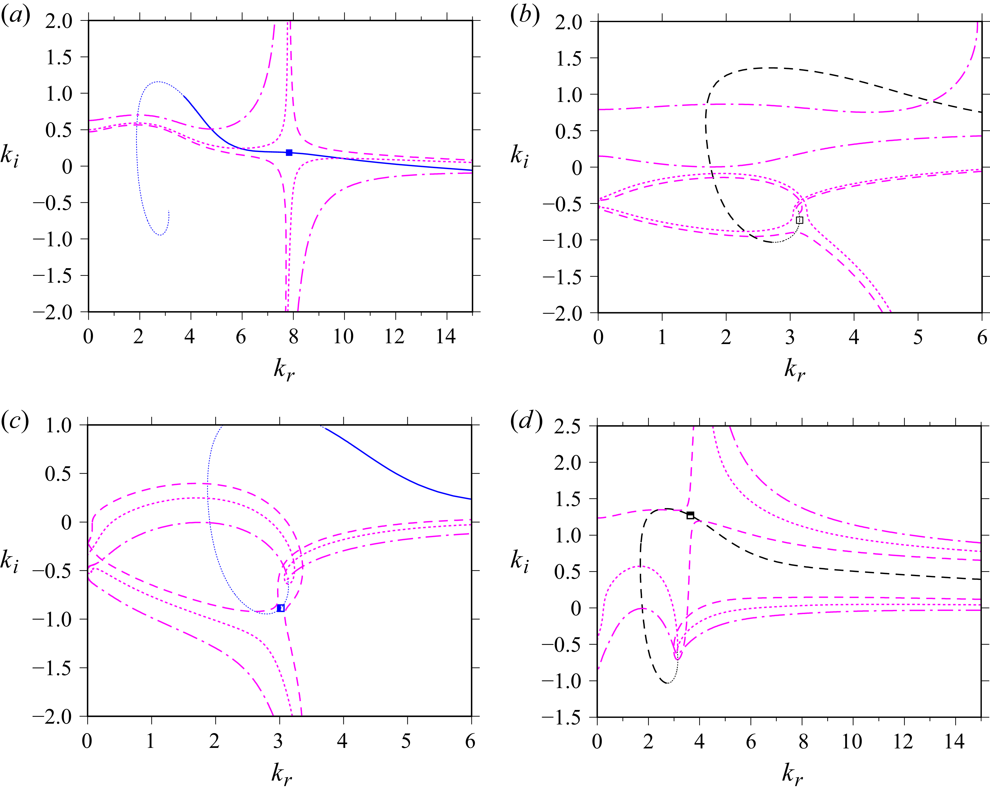


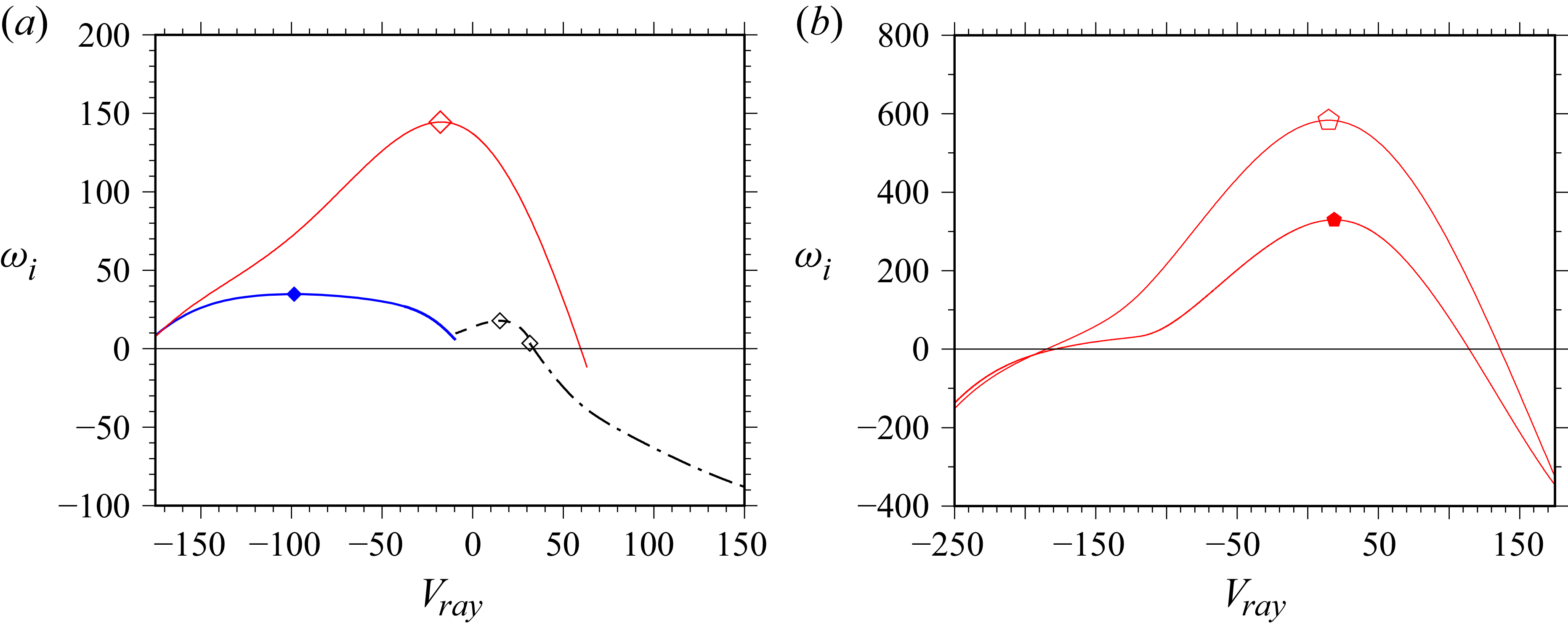


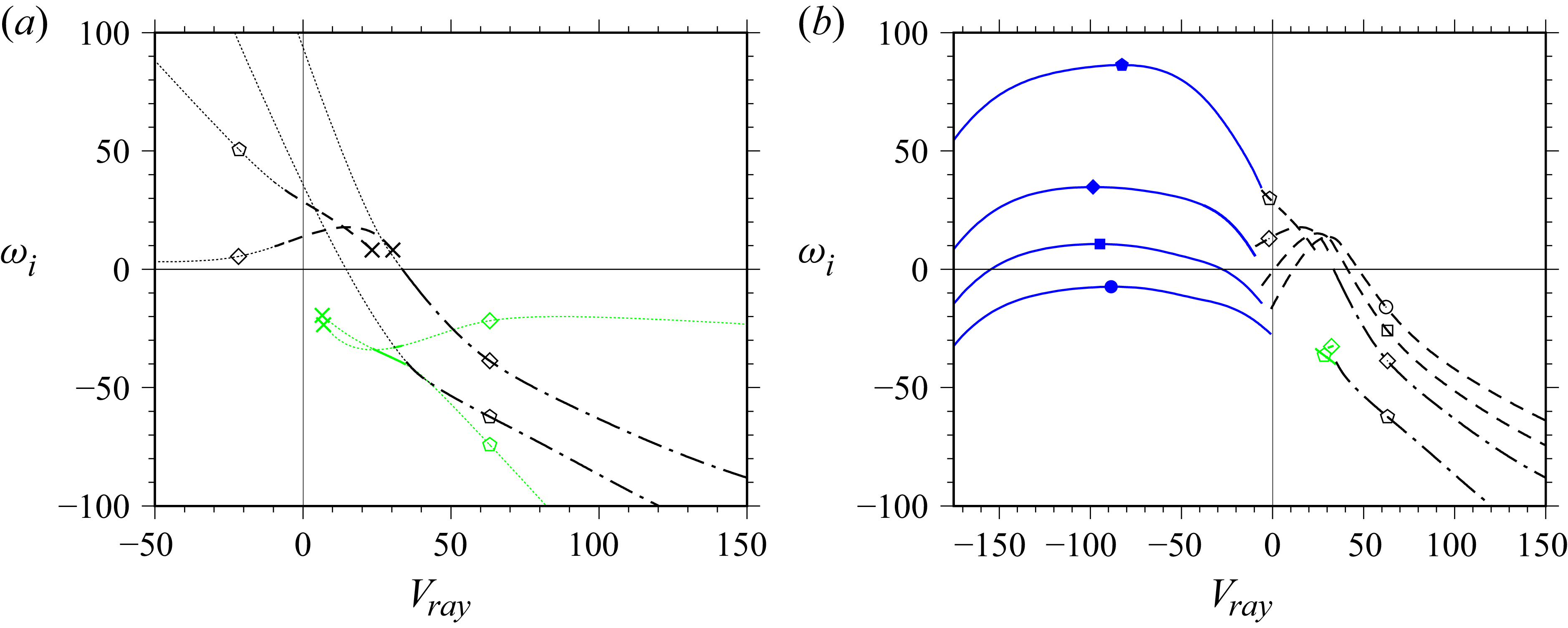


 Open access