


1. Introduction
A suspension of swimming micro-organisms is a prime example of an active fluid, in which the motions of the cells and those they generate in the ambient fluid are powered by the metabolic energy of the cells, and are therefore unconstrained by conservation of energy principles. Such suspensions arise widely, in natural bodies of water (e.g. oceans, lakes, puddles), in or on larger organisms (e.g. vertebrate intestines, lungs, mouths), in technological bioreactors (e.g. food processing, brewing, biofuels) and many other fields. The study of individual and collective behaviour among swimming micro-organisms has blossomed in recent years among microbiologists, fluid dynamicists and soft-matter physicists, and numerous fascinating phenomena and mechanisms have come to light. As fluid dynamicists, we are particularly interested in developing theoretical approaches that shed light on the physical mechanisms concerned, in a manner that will explain laboratory or field observations as fully as possible.
Some of the interesting observations that have been made on suspensions of swimming micro-organisms include some that occur independently of the proximity of external boundaries and others that depend on such features. The former include instabilities such as bioconvective and gyrotactic instabilities as well as those driven by the cells’ self-propulsion (Kessler Reference Kessler1985a; Pedley & Kessler Reference Pedley and Kessler1992; Hill & Pedley Reference Hill and Pedley2005; Bees Reference Bees2020; Simha & Ramaswamy Reference Simha and Ramaswamy2002; among many others). The latter include the tendency of individual microswimmers to swim towards a nearby rigid boundary (Lauga et al. Reference Lauga, DiLuzio, Whitesides and Stone2006; Berke et al. Reference Berke, Turner, Berg and Lauga2008; Denissenko et al. Reference Denissenko, Kantsler, Smith and Kirkman-Brown2012; Ishimoto & Gaffney Reference Ishimoto and Gaffney2013), shear-gradient-induced migration (Barry et al. Reference Barry, Rusconi, Guasto and Stocker2015; Vennamneni, Nambiar & Subramanian Reference Vennamneni, Nambiar and Subramanian2020) and, in a shear flow near a wall, to swim upstream, i.e. exhibit rheotaxis (Kaya & Koser Reference Kaya and Koser2012; Lauga Reference Lauga2020) all of which can be explained in terms of hydrodynamics. Suspensions of swimmers in a shear flow can exhibit an increase or a decrease in their effective shear viscosity, in a channel flow for example, depending on the cell shape (elongated or nearly spherical) and its mode of swimming (pushing from behind, like bacteria or sperm, or pulling from in front, like many motile algae) (Sokolov & Aranson Reference Sokolov and Aranson2009; Subramanian & Koch Reference Subramanian and Koch2009; Rafaï, Jibuti & Peyla Reference Rafaï, Jibuti and Peyla2010; López et al. Reference López, Gachelin, Douarche, Auradou and Clément2015). An instructive review was given by Saintillan (Reference Saintillan2018). However, most of the analyses of the above phenomena concentrate primarily on the interaction between the swimming cells and the fluid, which implies that cell–cell interactions are not considered and the suspensions are taken to be dilute, with small volume fraction. In this paper we are concerned with concentrated suspensions, of large volume fraction, in a Newtonian fluid in which inertia is negligible. In the context of passive particles, the study of suspension rheology has a substantial literature (the reader is recommended to study the review by Guazzelli & Pouliquen Reference Guazzelli and Pouliquen2018).
The theoretical analysis of passive suspensions began with Einstein (Reference Einstein1906), who calculated the first correction to the molecular viscosity for a dilute suspension of identical rigid spheres, at small volume fraction  $\phi$, taking account of the fact that an isolated rigid sphere in a shear flow cannot deform in the same way that the fluid would if the sphere were not there, leading to
 \begin{equation} \mu_{eff} = \mu_0 \left(1 + \tfrac{5}{2} \phi \right), \end{equation}
where  $\mu _0$ is the viscosity of the suspending fluid. Batchelor (Reference Batchelor1970) initiated rigorous analysis of the stress system in a suspension of rigid spheres in which the configuration of particles is random and a particle's interaction with its neighbours influences the stress that it experiences. Batchelor considered semi-dilute suspensions, in which pairwise (nearest neighbour) interactions were fully incorporated. This analysis allowed Batchelor & Green (Reference Batchelor and Green1972a,Reference Batchelor and Greenb) to evaluate the effective viscosity of a suspension in a shear flow to second order in $\phi$; after some subsequent correction the effective viscosity, to order $\phi ^2$, is
 \begin{equation} \mu_{eff} = \mu_0 \left( 1+\tfrac{5}{2}\phi + K\phi^2 \right), \end{equation}
where the constant  $K$ is equal to $6.95$ for a pure straining flow. For a unidirectional shearing flow, we take the approximate value suggested by the following quote from page 3 of Guazzelli & Pouliquen (Reference Guazzelli and Pouliquen2018): ‘Assuming a random microstructure leads to a smaller coefficient $K\approx 5.0$ of $\phi ^2$. This latter expression seems to agree reasonably with the experimental data in the semi-dilute regime (up to $\phi \approx 0.10\unicode{x2013}0.15$)’. For more concentrated suspensions, especially in bounded domains, it is necessary to analyse hydrodynamic interactions between more than two spheres, which is conceptually and mathematically much more complicated, mainly because the velocity field of a particle, subject to an external force, falls off very slowly with distance $r$ from the particle, proportionally to $r^{-1}$, and the boundary conditions have to be imposed on complex geometries. It was therefore necessary to develop appropriate computational methods, of which the method of Stokesian dynamics is perhaps the most versatile (Brady & Bossis Reference Brady and Bossis1988; Brady et al. Reference Brady, Phillips, Lester and Bossis1988; Sierou & Brady Reference Sierou and Brady2002). The method was first applied to pressure-driven flow in a channel by Nott & Brady (Reference Nott and Brady1994), the plane channel walls being replaced by rows of equal spheres, each in contact with its neighbour, which were constrained all to move with the same velocity, viz. zero. The suspension average velocity is specified as a boundary condition, which is equivalent to prescribing the volumetric flow rate per unit cross-section, requiring a particular pressure gradient and hence leading to a particular effective viscosity. Nott and Brady found that particles tended to migrate toward the centre line of the channel, by the mechanism of shear-induced particle migration, which had been discovered and explained by Eckstein, Bailey & Shapiro (Reference Eckstein, Bailey and Shapiro1977) and by Leighton & Acrivos (Reference Leighton and Acrivos1987). For a concentrated suspension, the migration leads to a flattening of the mean velocity profile in the centre of the channel, and consequently to higher shear rate at the wall and hence to higher effective viscosity.
The effective viscosity of a suspension, even of identical rigid spheres, is found not to depend only on  $\phi$, but also on the velocity field itself, when the fluid domain is confined. That is to say that the suspension behaves like a non-Newtonian fluid with variable rheology. Moreover, when the concentration is high enough it becomes apparent that collisions with the wall of randomly moving particles mean that a particle pressure is exerted on the walls of the container (channel) (see Guazzelli & Pouliquen Reference Guazzelli and Pouliquen2018, § 3.1). In our modelling, contact between close neighbours is avoided by the introduction of a short-range, repulsive force, thereby preventing the suspension from jamming.
Our interest is also in analysing Poiseuille flow of a suspension in a channel, but made up of swimming micro-organisms, not inert particles. Swimming cells come in a myriad of shapes, but in order to build on the current understanding of concentrated suspensions of passive spheres, we will restrict our attention to spherical models of swimmers, i.e. squirmers (Lighthill Reference Lighthill1952; Blake Reference Blake1971; Pedley Reference Pedley2016). These keep their spherical shape and swim by means of an imposed, axisymmetric, tangential velocity distribution on the surface of the sphere, as set out in § 2.1 below. In our previous paper (Ishikawa, Brumley & Pedley Reference Ishikawa, Brumley and Pedley2021), the Stokesian dynamics method was used to compute the particle motions and the rheology, in particular the effective viscosity, of a monolayer of squirmers (cell centres and velocities confined to a plane) subjected to simple shear flow bounded by two parallel planes perpendicular to the monolayer, as in plane Couette flow. In that paper, the results were compared with those obtained on the assumption that the dynamic stresses in a concentrated suspension would be dominated by the thin lubrication layers between the squirmers, and the far-field dynamics would be unimportant. The conclusion was that lubrication theory was sufficiently accurate at high concentration (measured by the areal fraction in the plane of the monolayer), thereby providing a useful foundation for studies in which the collective dynamics is studied through lubrication interactions alone (Brumley & Pedley Reference Brumley and Pedley2019). At the same time, recent work demonstrates that lubrication theory and Stokesian dynamics provide similar results for pairs of squirmers interacting hydrodynamically (Darveniza et al. Reference Darveniza, Ishikawa, Pedley and Brumley2022). A fortiori, as the volume fraction increases, so that a given squirmer interacts with more than one other squirmer, the error in using lubrication theory, and hence Stokesian dynamics, instead of the full boundary element simulation, will diminish.
In this paper, we follow Nott & Brady (Reference Nott and Brady1994) and use fully three-dimensional Stokesian dynamics for a suspension of squirmers in a bumpy channel (with walls made up of a layer of rigid spheres stuck together), driven by a pressure gradient. This method is chosen to maximise computational accuracy, and provide a reference dataset for suspension rheology in Poiseuille flow. Since it is hard to specify pressure at the ends of a finite channel, we follow Nott & Brady in using an inverse method, specifying the mean, bulk longitudinal velocity in the channel, computing the longitudinal component of the wall shear stress and thereby inferring the pressure gradient and the effective viscosity; details are given in § 2.
It is well known that many micro-swimmers are bottom heavy and therefore experience a gravitational torque when their swimming direction is not oriented vertically. As in our earlier, semi-dilute, modelling of unconfined suspensions (Ishikawa & Pedley Reference Ishikawa and Pedley2007), we compute the consequent effect of gravity on the suspension rheology when the mean flow direction is vertical as well as horizontal. In this paper, the mean mass density of a squirmer is taken to be the same as that of the fluid, so there is no external body force on a squirmer and therefore no sedimentation.
An outline of the paper is as follows. The problem is specified mathematically and the Stokesian dynamics method summarised in § 2. Results for non-bottom-heavy squirmers in comparison with inert spheres, up to a volume fraction of  $\phi =0.45$ (recall that rigid spheres jam at $\phi = 0.58 \sim 0.65$) are given in § 3. The corresponding results for squirmers that are bottom heavy are given in § 4. It is of interest that bottom heaviness introduces much more significant non-Newtonian effects for the suspension as a whole, including normal stress differences and negative effective viscosity, than squirmers that do not experience an external torque. Finally, conclusions are provided in § 5.
2. Basic equations and numerical method
The methodology employed in this study is similar to our former study on a sheared suspension of squirmers (Ishikawa et al. Reference Ishikawa, Brumley and Pedley2021). The basic equations of Stokesian dynamics for simulating a suspension of squirmers were developed by Ishikawa, Locsei & Pedley (Reference Ishikawa, Locsei and Pedley2008) and those for including a wall boundary were developed by Nott & Brady (Reference Nott and Brady1994), so we explain the methodology only briefly here.
2.1. Squirmer
Active particles are modelled as identical steady spherical squirmers (Lighthill Reference Lighthill1952; Blake Reference Blake1971; Ishikawa, Simmonds & Pedley Reference Ishikawa, Simmonds and Pedley2006; Pedley Reference Pedley2016). The squirmer model has been utilised to analyse ciliated microorganisms, active colloids and droplets (Ishikawa & Pedley Reference Ishikawa and Pedley2023; Ishikawa Reference Ishikawa2024). Squirmers have radius  $a$ and swim by means of a prescribed tangential velocity on the surface
 \begin{equation} u_{\theta} = \tfrac{3}{2}V_s\sin{\theta}(1 + \beta\cos{\theta}), \end{equation}
where  $\theta$ is the polar angle from the squirmer's orientation vector $\boldsymbol {p}$, $V_s$ is the swimming speed and $\beta$ is the ratio of the second mode to the first squirming mode, which represents the stresslet strength. The squirmers may be bottom heavy, so that when the squirmer's orientation ${\boldsymbol {p}}$ is not vertical, the squirmer experiences a gravitational torque $\boldsymbol {T}$ given by
 \begin{equation} \boldsymbol{T} ={-}\rho \upsilon h \boldsymbol{p}\times \boldsymbol{g}. \end{equation}
Here,  $\upsilon$ is the cell volume, $h$ is the displacement of the centre of mass from the geometric centre, $\boldsymbol {g}$ is the gravitational acceleration and $\rho$ is the average density of the squirmer, assumed to be the same as that of the fluid.
The squirmer model has been verified by comparison with the experiments on microalgae Volvox (Ishikawa et al. Reference Ishikawa, Pedley, Drescher and Goldstein2020) and ciliates Paramecium (Ishikawa & Hota Reference Ishikawa and Hota2006) and Tetrahymena (Manabe, Omori & Ishikawa Reference Manabe, Omori and Ishikawa2020). The spherical squirmer model used in this study can represent ciliated microorganisms with a round shape. The actual microbial values of  $\beta$ are approximately 0.28 for Paramecium caudatum (Ishikawa & Hota Reference Ishikawa and Hota2006) and very small for Volvox carteri (Short et al. Reference Short, Solari, Ganguly, Powers, Kessler and Goldstein2006). Thus, P. caudatum can be modelled as a puller squirmer, while V. carteri can be modelled as a neutral squirmer. (It is of course clear that the squirmer model is highly idealised and will not be directly applicable to the majority of microorganism species, which have a multitude of shapes such as elongated bacteria or multifaceted diatoms, and may be deformable.)
2.2. Problem settings
We consider Poiseuille flow of an infinite suspension of squirmers between two parallel walls, as shown in figure 1( $a$). Poiseuille flow is driven by the pressure gradient in the $x$-direction: the $y$-axis is taken perpendicular to the wall, and the $z$-axis is taken as the spanwise direction. The unit domain is a rectangular parallelepiped with side lengths $L_x$, $L_y$ and $L_z$, and three-dimensional periodic boundary conditions are applied to reflect the infinite suspension. The parallel walls consist of a two-dimensional hexagonal lattice of fixed rigid spheres with the same radius as the squirmers, i.e. wall spheres. The inner distance between the walls is $H$ (
$H$ ( $=L_y - 2a$). The methodology to express a wall boundary by wall spheres was employed by Nott & Brady (Reference Nott and Brady1994), in which Poiseuille flow of an infinite suspension of rigid spheres was simulated by Stokesian dynamics. Although there will be a small quantitative effect of having bumpy walls, the qualitative behaviour of the system is expected to remain unchanged, because the lubrication forces between a wall and a squirmer and that between a sphere and a squirmer are essentially the same equation, just with different coefficients (Kim & Karrila Reference Kim and Karrila2005; Ishikawa et al. Reference Ishikawa, Simmonds and Pedley2006; Ishikawa Reference Ishikawa2019).
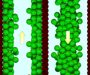
Poiseuille flow of a suspension of non-bottom-heavy neutral squirmers ( $\beta =0$). ( $a$) Problem setting of the simulation. Poiseuille flow of an infinitely periodic suspension of squirmers with $\phi =0.1$, which is driven by a pressure gradient in the $x$-direction: the $y$-axis is taken perpendicular to the wall, and the $z$-axis is taken as the spanwise direction. The unit domain is a rectangular parallelepiped with side lengths $L_x, L_y$ and $L_z$. Two parallel walls consist of two-dimensional hexagonal lattices of rigid spheres, and the inner distance between the walls is $H$. Green spheres represent squirmers: the red region represents the anterior part and the white line indicates the equator. ( $b$) Sample image of squirmer distribution with $\phi =0.45$ (see supplementary movie 1 available at https://doi.org/10.1017/jfm.2024.1205). The yellow arrow indicates the flow direction. ( $c$) Time-dependent longitudinal force acting on the wall spheres, $\bar {F}_w$, for four different volume fractions of squirmers. The pressure drop can be calculated as $-{\rm d}P/{{\rm d}\kern 0.06em x} = (N_w/L_x L_y L_z) \bar {F}_w$, where $N_w$ is the number of wall spheres in the unit domain. ( $d$) Time series of the parameter, $N_s^{+y}/N_s$, for various volume fractions, where $N_s$ is the number of squirmers in the unit domain, and $N_s^{+y}$ is the number of squirmers in half the simulation domain where the $y$-coordinate is positive. For a uniform distribution, $N_s^{+y}/N_s = 0.5$.

In this setting, the velocities of the wall spheres and the forces on the interior squirmers are prescribed, leaving the velocities of the squirmers and the forces on the wall spheres to be determined. The interior squirmers are force free and subjected to a torque, as described by (2.2). If we set a fixed average suspension velocity  $\langle \boldsymbol {u} \rangle$ then a pressure gradient will be set up so as to satisfy the global conservation of momentum (Nott & Brady Reference Nott and Brady1994). We specify that the wall spheres are stationary, so the force required to hold these spheres stationary will balance the pressure gradient needed to maintain the non-zero average $\langle \boldsymbol {u} \rangle$. The average $x$-direction force acting on the wall spheres $\bar {F}_w$ is given as
 \begin{equation} \bar{F}_w = \frac{1}{N_w} \sum_{i=1}^N \boldsymbol{F}_w^{(i)} |_{x} , \end{equation}
where  $N_w$ is the number of wall spheres in the unit domain, and $\boldsymbol {F}_w^{(i)} |_{x}$ is the $x$-direction force acting on wall sphere $i$. Considering the global conservation of momentum, the pressure drop in the $x$-direction can be directly derived from $\bar {F}_w$ as
 \begin{equation} {-}\frac{{\rm d}P}{{\rm d}\kern 0.06em x} = \frac{N_w}{L_x L_y L_z} \bar{F}_w . \end{equation}
 In § 4, gravity is introduced for bottom-heavy squirmers. Although the  $x$-axis is taken in the flow direction in § 3, it is taken to be vertically upward in § 4. The gravitational direction is thus $-\boldsymbol {x}$, and flow in the positive $x$-direction is called upflow, while flow in the negative $x$-direction is called downflow in § 4.
2.3. Stokesian dynamics
Assuming that squirmers and the channel height are sufficiently small, we neglect inertia. The hydrodynamic interactions among squirmers and wall spheres at negligible inertia are calculated by Stokesian dynamics (Brady & Bossis Reference Brady and Bossis1988; Brady et al. Reference Brady, Phillips, Lester and Bossis1988; Nott & Brady Reference Nott and Brady1994; Ishikawa et al. Reference Ishikawa, Locsei and Pedley2008). An infinite extent of the suspension is computed by the Ewald summation technique (Beenakker Reference Beenakker1986). By exploiting the Stokesian dynamics method, the force  $\boldsymbol {F}$, torque $\boldsymbol {T}$ and stresslet ${\boldsymbol {S}}$ of squirmers and wall spheres are given by
 \begin{align} \left(\!\! \begin{array}{c} \boldsymbol{F}_s \\ \boldsymbol{F}_w \\ \boldsymbol{T}_s \\ \boldsymbol{T}_w \\ {\boldsymbol{\mathsf{S}}}_s \\ {\boldsymbol{\mathsf{S}}}_w \end{array}\! \!\right) &= \left[ {\boldsymbol{\mathsf{R}}}^{far} - {\boldsymbol{\mathsf{R}}}_{2B}^{far} + {\boldsymbol{\mathsf{R}}}_{2B}^{near} \right] \left( \!\!\begin{array}{c} \boldsymbol{U}_s - \langle \boldsymbol{u} \rangle \\ \boldsymbol{U}_w - \langle \boldsymbol{u} \rangle \\ \boldsymbol{\varOmega}_s - \langle \boldsymbol{\omega} \rangle \\ \boldsymbol{\varOmega}_w - \langle \boldsymbol{\omega} \rangle \\ - \langle {\boldsymbol{\mathsf{E}}} \rangle \\ - \langle {\boldsymbol{\mathsf{E}}} \rangle \end{array}\!\!\right) \nonumber\\ &\quad + \left[ {\boldsymbol{\mathsf{R}}}^{far} - {\boldsymbol{\mathsf{R}}}_{2B}^{far} \right] \left( \!\!\begin{array}{c} - V_s \boldsymbol{p} + {\boldsymbol{\mathsf{Q}}}_{s} \\ 0 \\ 0 \\ 0 \\ - \dfrac{3}{10}V_s \beta \left( 3 \boldsymbol{pp} - {\boldsymbol{\mathsf{I}}} \right) \\ 0 \end{array} \!\!\right) + \left( \!\!\begin{array}{c} \boldsymbol{F}_{s}^{near} \\ \boldsymbol{F}_{w}^{near} \\ \boldsymbol{T}_{s}^{near} \\ \boldsymbol{T}_{w}^{near} \\ {\boldsymbol{\mathsf{S}}}_{s}^{near} \\ {\boldsymbol{\mathsf{S}}}_{w}^{near} \end{array} \!\!\right) , \end{align}
where  ${\boldsymbol{\mathsf{R}}}$ is the resistance matrix, $\boldsymbol {U}$ and $\boldsymbol { \varOmega }$ are the translational and rotational velocities of a squirmer, $\langle \boldsymbol {u} \rangle$ and $\langle \boldsymbol {\omega } \rangle$ are the translational and rotational velocities of the bulk suspension and $\langle {\boldsymbol{\mathsf{E}}} \rangle$ is the rate of strain tensor of the bulk suspension. The index $s$ or $w$ represents a squirmer or a wall sphere, respectively. Here, $\boldsymbol{\mathsf{Q}}_s$ is the irreducible quadrupole providing additional accuracy, which is approximated by its mean-field value (Brady et al. Reference Brady, Phillips, Lester and Bossis1988). The brackets $(~)$ and $[~]$ indicate a vector and a matrix, respectively. Index far or near indicates far- or near-field interaction, and 2B indicates interaction between two inert spheres. Wall spheres are fixed in space, so we have $\boldsymbol {U}_w = \boldsymbol {\varOmega }_w = 0$. The bulk rotational velocity $\langle \boldsymbol {\omega } \rangle$ and shear rate $\langle {\boldsymbol{\mathsf{E}}} \rangle$ are set to zero as the flow is driven by the pressure gradient in the suspension. The near-field forces and stresslets in the last term on the right side are obtained computationally using a boundary element method (Ishikawa et al. Reference Ishikawa, Simmonds and Pedley2006).
The governing equation for the squirmer motion can be derived from (2.5) as
 \begin{equation} \left( \!\!\begin{array}{c} \boldsymbol{F}_s \\ \boldsymbol{T}_s \end{array} \!\!\right) = \left[ {\boldsymbol{\mathsf{R}}}^{far} - {\boldsymbol{\mathsf{R}}}_{2B}^{far} + {\boldsymbol{\mathsf{R}}}_{2B}^{near} \right]_{FUss} \left( \!\!\begin{array}{c} \boldsymbol{U}_s - \langle \boldsymbol{u} \rangle \\ \boldsymbol{\varOmega}_s \end{array} \!\!\right) + \left( \!\!\begin{array}{c} \boldsymbol{F}_{c} \\ \boldsymbol{T}_{c} \end{array} \! \! \right) , \end{equation}
where
 \begin{align} \left( \! \! \begin{array}{c} \boldsymbol{F}_{c} \\ \boldsymbol{T}_{c} \end{array} \! \! \right) &= \left[ {\boldsymbol{\mathsf{R}}}^{far} - {\boldsymbol{\mathsf{R}}}_{2B}^{far} + {\boldsymbol{\mathsf{R}}}_{2B}^{near} \right]_{FUsw} \left( \! \! \begin{array}{c} - \langle \boldsymbol{u} \rangle \\ 0 \end{array} \! \! \right) \nonumber\\ &\quad + \left[ {\boldsymbol{\mathsf{R}}}^{far} - {\boldsymbol{\mathsf{R}}}_{2B}^{far} \right]_{FUSss} \left( \! \! \begin{array}{c} \! - V_s \boldsymbol{p} + {\boldsymbol{\mathsf{Q}}}_{s} \\ 0 \\ - \dfrac{3}{10}V_s \beta \left( 3 \boldsymbol{pp} - {\boldsymbol{\mathsf{I}}} \right) \end{array} \! \! \right) + \left( \! \! \begin{array}{c} \boldsymbol{F}_{s}^{near} \\ \boldsymbol{T}_{s}^{near} \end{array} \right) . \end{align}
Index FUss or FUsw indicates force–velocity interaction with a squirmer or a wall sphere, FUSss indicates force–velocity-stresslet interaction with a squirmer, respectively. This equation is solved for  $\boldsymbol {U}_s$ and $\boldsymbol {\varOmega }_s$ under given $\boldsymbol {F}_s$ and $\boldsymbol {T}_s$ conditions.
Once the velocities of squirmers are obtained, the force exerted on a wall sphere can be calculated by
 \begin{align} \left( \!\!\begin{array}{c} \boldsymbol{F}_w \\ \boldsymbol{T}_w \end{array} \!\!\right) &= \left[ {\boldsymbol{\mathsf{R}}}^{far} - {\boldsymbol{\mathsf{R}}}_{2B}^{far} + {\boldsymbol{\mathsf{R}}}_{2B}^{near} \right]_{FUww} \left( \!\!\begin{array}{c} - \langle \boldsymbol{u} \rangle \\ 0 \end{array}\!\! \right) \nonumber\\ &\quad +\left[ {\boldsymbol{\mathsf{R}}}^{far} - {\boldsymbol{\mathsf{R}}}_{2B}^{far} + {\boldsymbol{\mathsf{R}}}_{2B}^{near} \right]_{FUws} \left( \!\!\begin{array}{c} \boldsymbol{U}_s - \langle \boldsymbol{u} \rangle \\ \boldsymbol{\varOmega}_s \end{array}\!\! \right) \nonumber\\ &\quad+ \left[ {\boldsymbol{\mathsf{R}}}^{far} - {\boldsymbol{\mathsf{R}}}_{2B}^{far} \right]_{FUSws} \left( \!\!\begin{array}{c} - V_s \boldsymbol{p} + {\boldsymbol{\mathsf{Q}}}_{s} \\ 0 \\ - \dfrac{3}{10}V_s \beta \left( 3 \boldsymbol{pp} - {\boldsymbol{\mathsf{I}}} \right) \end{array} \!\!\right) +\left( \!\!\begin{array}{c} \boldsymbol{F}_{w}^{near} \\ \boldsymbol{T}_{w}^{near} \end{array} \!\!\right) . \end{align}
Index FUws or FUww indicates force–velocity interaction with a squirmer or a wall sphere, FUSws indicates force–velocity-stresslet interaction with a squirmer, respectively.
2.4. Numerical method
We set a fixed average suspension velocity as  $\langle \boldsymbol {u} \rangle = ( \bar {u}, 0, 0)$. In the case of downflow in § 4, however, the fixed average suspension velocity is set as $( -\bar {u}, 0, 0)$. We also specify that the wall spheres are stationary, so the force required to hold these spheres stationary will balance the pressure gradient needed to maintain $\langle \boldsymbol {u} \rangle$.
The unit domain is a rectangular parallelepiped with side lengths  $L_x = 11.3a, L_y = 15.1a$ and $L_z = 5.66a$, although the channel height, $L_y$, is changed in figure 5. Three-dimensional periodic boundary conditions are applied to represent the infinite suspension, and these are computed by the Ewald summation technique (Beenakker Reference Beenakker1986). In the unit domain, the wall consists of 16 wall spheres placed in a two-dimensional hexagonal lattice. The volume fraction of squirmers, $\phi$, is varied in the range $0.1$ to $0.45$, which corresponds to the number of squirmers in the unit domain varying from 20 to 90. Initially, squirmers are placed randomly in position and orientation. Because of the difficulty of using random numbers for placement under high $\phi$ conditions, we used a random arrangement that initially allowed particles to overlap and then eliminated the overlap by generating repulsion between particles as the initial configuration. The dynamic motions afterwards are calculated by the fourth-order Adams–Bashforth time-marching scheme with a time step of $5 \times 10^{-4} a/V_s$.
A non-hydrodynamic interparticle short-range repulsive force,  $\boldsymbol {F}_{rep}$, is added to the system in order to avoid the prohibitively small time step needed to overcome the problem of overlapping particles. We will follow Ishikawa et al. (Reference Ishikawa, Locsei and Pedley2008), and use the following function:
 \begin{equation} \boldsymbol{F}_{rep} = \alpha_1 \frac{\alpha_2 \exp(-\alpha_2 \varepsilon)} {1-\exp(-\alpha_2 \varepsilon)} \frac{\boldsymbol{r}}{r}, \end{equation}
where  $\alpha _1$ is a dimensional coefficient, $\alpha _2$ is a dimensionless coefficient and $\varepsilon$ is the minimum separation between particle surfaces, non-dimensionalised by their radius. Here, $\boldsymbol {r}$ is the vector connecting the centres of two spheres, and $r = |\boldsymbol {r}|$. The coefficients used in this study are $\alpha _1 = \alpha _2 = 100$, so that the minimum $\varepsilon$ obtained with these parameters is of the order of $10^{-3}$.
There are two important dimensionless parameters in addition to  $\beta$ and $\phi$: $G_{bh}$ and $Sq$. The value of $G_{bh}$ is proportional to the ratio of the time to swim a body length to the time to rotate to face upwards, and is defined as
 \begin{equation} G_{bh}=\frac{4 {\rm \pi}\rho g a h}{3 \mu V_s} . \end{equation}
The parameter  $G_{bh}$ is varied from 0 to 100. The parameter $Sq$ is the swimming speed, scaled with a background velocity, i.e.
 \begin{equation} Sq = \frac{V_s}{\bar{u}}. \end{equation}
Here,  $Sq$ is equal to 1 except in figure 4(f). The squirming parameter $\beta$ is varied in the range $-3$ to $3$.
$3$.
Time-averaged quantities are evaluated in the range  $20 \leqslant t (\bar {u}/a) \leqslant 150$, as shown in figures 1(c) and 1(d). All data points are the average of three independent simulations with different initial conditions. Error bars in the figures represent the standard deviation of the time variation, averaged over the three cases. The ratio of the force acting on the wall spheres in the presence of squirmers, to that in the absence of squirmers, i.e. $\bar {F}_w/\bar {F}_{w,0}$, is equivalent to the pressure drop relative to that without squirmers. It is also equivalent to the effective viscosity relative to the fluid viscosity as
 \begin{equation} \mu_{eff} = \mu_0 \frac{\bar{F}_w}{\bar{F}_{w,0}} . \end{equation}
Thus, we will plot  $\bar {F}_w/\bar {F}_{w,0}$ and discuss the effect of squirmers on the pressure drop and effective viscosity.
3. Results for non-bottom-heavy squirmers
To begin with, we examined how long it takes for the Poiseuille flow to reach a steady state. Figures 1(a) and 1(b) show the distribution of non-bottom-heavy neutral squirmers ( $\beta =G_{bh}=0$) at 130 time units with volume fractions of $\phi =0.1$ and $\phi =0.45$, respectively (cf. supplementary movie 1). The yellow arrow in the figure indicates the flow direction. We see that many squirmers in figure 1(a) ( $\phi =0.1$) orient upstream and show rheotaxis. The time change of the force acting on the wall spheres, $\bar {F}_w$, is shown in figure 1(c). The forces fluctuate considerably throughout the computation, but after approximately 20 time units, there is no significant change in the average value for approximately 50 time units for any volume fraction. Figure 1(d) shows the time change of $N_s^{+y}/N_s$, where $N_s$ is the number of squirmers in the unit domain, and $N_s^{+y}$ is the number of squirmers in half the simulation domain where the $y$-coordinate is positive. For a uniform distribution, we would have $N_s^{+y}/N_s = 0.5$. The results indicate, especially for the low volume fraction, that a group of squirmers travels back and forth between the parallel walls. There are two important swimming tendencies for neutral squirmers: ( $a$) a solitary neutral squirmer tends to swim away from a wall (Ishikawa Reference Ishikawa2019), and ( $b$) neutral squirmers tend to swim in the same direction as surrounding squirmers (Ishikawa et al. Reference Ishikawa, Locsei and Pedley2008). The first tendency generates reflections of squirmers between two walls and the second tendency induces the group swimming of squirmers. In the present study, both tendencies occur simultaneously, resulting in the large-scale wall-to-wall clustering motion. Similar large-scale wall-to-wall clustering motion was also reported for weak pullers with $\beta = 0.5$ (Oyama, Molina & Yamamoto Reference Oyama, Molina and Yamamoto2016). The time scale it takes to travel to the opposite wall is approximately 20 time units. Considering these results, we decided to average the force acting on the wall spheres, $\bar {F}_w$, from 20 to 150 time units.
3.1. Comparison with inert sphere suspensions
In this section, we compare the behaviour of non-bottom-heavy neutral squirmers ( $\beta =G_{bh}=0$) with that of inert spheres. Figure 2(a) shows the velocity distribution of inert spheres in the Poiseuille flow. The broken line in the figure indicates the parabolic velocity profile of a Newtonian fluid, situated between two flat plates which are separated by distance $H$. In the present study, the wall is not flat but consists of spheres, so a small amount of fluid flows in the wall region where $|y|>H/2$. Thus, the velocity distribution becomes a little slower than the analytical solution assuming the wall is at $y= \pm H/2$. In the dilute limit of $\phi = 0.005$, the velocity distribution of inert spheres is almost parabolic, indicating the reliability of the present methodology. In the concentrated suspension with $\phi = 0.45$, the velocity distribution across the channel exhibits deviations away from a smooth profile (see figure 2a). This is because inert spheres in the concentrated suspension form layers, as shown in figure 2(b), and the particle distribution is not uniform (see supplementary movie 2). The distribution of particles can be biased in the $y$-direction at any instant in time, but the bias is removed when averaging over 20–150 time units. Hence, the probability density distribution is averaged to be symmetric in the $y>0$ and $y<0$ regions. We see that seven layers exist within the distance $H=13.1a$ between the walls.
Comparison between suspensions of inert spheres (a,b) and squirmers (c,d). (a) Velocity distribution of inert spheres. The broken line indicates the parabolic velocity profile of a Newtonian fluid, situated between two flat plates which are separated by distance  $H$. (b) Probability density distribution of inert spheres, normalised by the average density. (c) Velocity distribution of squirmers. (d) Probability density distribution of squirmers, normalised by the average density.

In the case of a squirmer suspension, the velocity distribution is very different from that of the inert sphere suspension (figure 2c). Compared with inert spheres, squirmers are slower, and this trend is more pronounced at lower volume fractions. This result may seem counterintuitive. However, this is due to the fact that the squirmers are swimming in the upstream direction, i.e. they exhibit rheotaxis. Figure 3(c) shows the orientation of squirmers, where  $e_x$ is the $x$-component of the orientation vector and $e_x=-1$ indicates that the squirmer faces upstream. We see $e_x \sim -0.6$ when $\phi = 0.1$, indicating that the majority of neutral squirmers are facing upstream. Since these squirmers swim upstream, the velocity distribution becomes much slower than the analytical solution. As the volume fraction increases, the tendency to direct upstream is weakened by hydrodynamic interactions, resulting in a diminished velocity reduction in figure 2(c).
Effects of the volume fraction of squirmers  $\phi$ (for $\beta =0, G_{bh} = 0$). (a) Time change of $y$-position, $r_y$, for 20 squirmers in a suspension with $\phi =0.1$. (b) Time change of $r_y$ for 20 out of 90 squirmers in a suspension with $\phi =0.45$. (c) Orientation of squirmers, where $e_x$ is the $x$-component of the orientation vector. (d) Orientational correlation of nearby squirmers $\langle \boldsymbol {e}_i \boldsymbol {\cdot } \boldsymbol {e}_j \rangle _{r < 2.5a}$, where $\boldsymbol {e}_i$ and $\boldsymbol {e}_j$ are the orientation vectors of squirmers $i$ and $j$ that are within a distance of $2.5a$. (e) Pair distribution function of squirmers. (f) Ratio of the force acting on the wall spheres to that without particles, which is equivalent to the pressure drop relative to that without particles, as well as the effective viscosity relative to the fluid viscosity. The results of squirmer suspensions and inert sphere suspensions are plotted. The analytical solution for the effective viscosity of a dilute suspension of inert spheres is shown by the broken line (see (1.1)). The effective viscosity obtained in Ishikawa et al. (Reference Ishikawa, Brumley and Pedley2021) for a monolayer suspension of squirmers with $\beta =1$ in simple shear flow is also plotted for comparison, in which the volume fraction was calculated from the thickness and areal fraction of the monolayer.

Another striking difference is that squirmers do not form sustained layers as in the case for inert spheres: compare figure 2(d) with 2(b). The distribution of squirmers is close to homogeneous except near the walls because the squirmers continuously change position as they swim. Figure 3(a) shows the time change of the  $y$-position for 20 squirmers in the dilute suspension with $\phi =0.1$. Two squirmers remain near the wall, but many squirmers swim near the centre of the channel, facing upstream. Some of these tendencies have been reported in former studies on a single squirmer swimming in a channel (Zöttl & Stark Reference Zöttl and Stark2012; Qi et al. Reference Qi, Annepu, Gompper and Winkler2020). Thus, the tendency to remain close to the wall or to migrate to the channel centre, facing upstream, is considered a phenomenon that also appears for solitary squirmers. These tendencies are not observed when the volume fraction is as high as 0.45, as shown in figure 3(b). The reasons for this are that the squirmers cannot accumulate further due to the already high volume fraction, and the strong near-field hydrodynamic interactions disrupt the orientational order.
In order to examine the effects of interactions between squirmers, the orientational correlation of nearby squirmers  $\langle \boldsymbol {e}_i \boldsymbol {\cdot } \boldsymbol {e}_j \rangle _{r < 2.5a}$ is calculated, where $\boldsymbol {e}_i$ and $\boldsymbol {e}_j$ are the orientation vectors of squirmer $i$ and $j$ that are within a distance of $2.5a$. The results are presented in figure 3(d), which indicates that the correlation decreases as the volume fraction increases. The decreased correlation is related to the decrease in orientational order in figure 3(c). The pair distribution function of squirmers is plotted in figure 3(e). Values greater than 1 indicate that the probability density in the presence of particles is higher than in a uniform arrangement. As the volume fraction increases, the peak of the pair distribution function appears at smaller values of $r$ and the peak value increases. Consequently, the squirmers interact in the near field more strongly as the volume fraction increases, resulting in a reduction in orientational order.
Considering the global conservation of momentum, the pressure drop in the  $x$-direction can be derived from the force acting on the wall spheres, $\bar {F}_w$, using (2.4). Let $\bar {F}_{w,0}$ be the force acting on the wall spheres in the absence of suspended particles, i.e. $\phi =0$, so that the ratio $\bar {F}_{w} / \bar {F}_{w,0}$ indicates the pressure drop relative to that without particles. The ratio is also equivalent to the effective viscosity relative to the solvent viscosity. Thus, investigating the ratio $\bar {F}_{w} / \bar {F}_{w,0}$ is important in order to understand the rheological properties of suspensions in Poiseuille flow. Figure 3(f) shows the ratio of the force acting on the wall spheres to that without particles for squirmer suspensions and inert sphere suspensions. The analytical solution for the effective viscosity of a dilute suspension of inert spheres is shown by the broken line. The effective viscosity obtained in our former study (Ishikawa et al. Reference Ishikawa, Brumley and Pedley2021) for squirmers with $\beta =1$ in simple shear flow, instead of Poiseuille flow, is also plotted for comparison. The sheared suspension is a monolayer in a thin film with a thickness of about $2a$, which is different from two-dimensional and full three-dimensional suspensions. We see that the effective viscosity of squirmer suspensions is considerably larger than that of inert sphere suspensions. This could be due to stronger momentum exchange in the case of squirmers, since they do not form layers and there are stronger interactions between particles. The differences between Ishikawa et al. (Reference Ishikawa, Brumley and Pedley2021) and the present study are the inclusion of the no-slip walls, the extension of the configuration from a monolayer to three dimensions and consideration of Poiseuille flow as opposed to shear flow. At lower volume fractions, the effective viscosity of the Poiseuille flow is greater than that of Ishikawa et al. (Reference Ishikawa, Brumley and Pedley2021), which could be due to the closer interactions that appear in the present setting. In contrast, at higher volume fractions, the effective viscosity of Ishikawa et al. (Reference Ishikawa, Brumley and Pedley2021) increases more rapidly than that of the Poiseuille flow. This is because the maximum volume fraction attainable in a thin film monolayer in Ishikawa et al. (Reference Ishikawa, Brumley and Pedley2021) is approximately 0.58, calculated as $2{\rm \pi} /(3\sqrt {3} \times 2.1)$ using the film thickness of $2.1a$, whereas in our study it is approximately 0.74. The difference in the maximum volume fraction is due to the different degrees of freedom in the suspension configuration. Even at the same volume fraction, the clearance between spheres is narrower in the monolayer suspension than in the three-dimensional suspension, leading to stronger lubrication forces and higher viscosity.
3.2. Effects of swimming mode, swimming speed and wall distance
The squirming mode,  $\beta$, changes the behaviour of squirmers in Poiseuille flow. Figure 4(a) shows the orientation of non-bottom-heavy pusher squirmers with $\beta =-1$. We see that the tendency to face upstream is weaker than for neutral squirmers, though the tendency of puller squirmers was almost the same as neutral squirmers (data not shown). To examine the effects of interactions between squirmers, the orientational correlation of nearby squirmers and the pair distribution function of squirmers are plotted in figures 4(b) and 4(c), respectively. The orientational correlation is observed to diminish when $\beta =-3$ and $\phi =0.45$, as a consequence of strong hydrodynamic interactions. Given that the influence of $\beta$ on the pair distribution function of squirmers is relatively minor, it can be concluded that the squirming mode does not affect the positions of nearby squirmers, but rather the orientation of nearby squirmers.
Effects of the squirming mode,  $\beta$, and the dimensionless number, $Sq$, expressing the swimming speed relative to the background flow speed. Results are plotted for $G_{bh} = 0$. (a) Orientation of pusher squirmers with $\beta =-1$, where $e_x$ is the $x$-component of the orientation vector. (b) Orientational correlation of nearby squirmers $\langle \boldsymbol {e}_i \boldsymbol {\cdot } \boldsymbol {e}_j \rangle _{r < 2.5a}$, where $\boldsymbol {e}_i$ and $\boldsymbol {e}_j$ are the orientation vectors of squirmers $i$ and $j$ that are within a distance of $2.5a$ and the self-contribution ( $i = j$) is excluded. (c) Pair distribution function of squirmers. (d) Ratio of the force acting on the wall spheres to that without particles, i.e. the effective viscosity, for suspensions of puller squirmers ( $\beta =1$), neutral squirmers ( $\beta =0$), pusher squirmers ( $\beta =-1$) and inert spheres. (e) Effect of $\beta$ on the effective viscosity ( $\phi = 0.45$). (f) Effect of $Sq$ on the effective viscosity ( $\phi = 0.45$).

The ratio of the force acting on the wall spheres to that without particles, i.e. the effective viscosity, for suspensions of puller squirmers ( $\beta =1$), neutral squirmers ( $\beta =0$), pusher squirmers ( $\beta =-1$) and inert spheres is shown in figure 4(d). The effective viscosities of the squirmer suspensions are approximately twice as high as those of the inert sphere suspensions, but the difference due to the swimming mode $\beta$ is less pronounced. Figure 4(e) shows the effect of varying $\beta$ on the effective viscosity of a concentrated suspension, with $\phi = 0.45$. We see that pusher squirmer suspensions tend to be slightly more viscous than puller squirmer suspensions. This difference may be due to the fact that, compared with a puller squirmer, a pusher squirmer does not exhibit the same extent of upstream alignment, therefore resulting in more collisions between particles, which promote momentum transfer.
The swimming speed normalised by the background velocity  $\bar {u}$ is represented by $Sq$. Figure 4(f) shows the effect of $Sq$ on the effective viscosity with $\phi = 0.45$. The effective viscosity increases as $Sq$ is increased, because the momentum transport in the suspension is enhanced by swimming. The results for large $Sq$ are not plotted because the repulsive force used in this study could not prevent the squirmers from overlapping and the computation could not be continued stably. It is not clear why the effective viscosity with $Sq=3$ is smaller than that with $Sq=1$ for strong pushers (with $\beta =-3$). Further investigation is needed in the future, as past studies have reported different behaviour of squirmers at various values of $Sq$ (see Qi et al. Reference Qi, Annepu, Gompper and Winkler2020).
Figure 5 shows the effects of varying the wall separation distance,  $H$, under the conditions of $\phi =0.3$ and $\beta = G_{bh} = 0$. Here, $H = 13.1a$ is the original distance, and the modified distance is varied from $7.1a$ to $19.2a$. The velocity distribution is flattened more in a narrower channel and is closer to parabolic in a wider channel (figure 5a). The spatial variation in the mean squirmer orientation changes as shown in figure 5(b), with a narrower channel showing a more pronounced tendency to face upstream. These results indicate that the tendency for a squirmer to orient upstream appears as a result of interactions with the wall spheres. In the case of the wider channel with $H=19.2a$, there is a tendency for squirmers to face upstream near the wall, but this effect weakens with distance from the wall. This result also suggests that, in addition to the background flow and the cell swimming, interactions with a wall play an important role in the emergence of rheotaxis. In a narrower channel, squirmers are directed more upstream, so the velocity distribution is flatter, with lower velocities around the centre. The probability density distribution of squirmers, normalised by the average density, is shown in figure 5(c) (compare figure 2d) The normalised probability density near the wall is higher in a wider channel because, for the same volume fraction, a wider channel has a greater number of squirmers in it, which tend to gather near the walls. These results clearly illustrate that the number of squirmers that accumulate near the wall depends on the wall separation distance (domain size). The number of accumulated squirmers increases in proportion to $H$, so the number of wall layers of squirmers also increases with $H$.
$H$.
Effects of varying the distance between walls (for  $\phi =0.3$, $\beta =0$, $G_{bh} = 0$). Here, $H = 13.1a$ is the original distance, and the modified distance is varied from $7.1a$ to $19.2a$. (a) Velocity distribution of squirmers. The broken line indicates the parabolic velocity profile for a Newtonian fluid. (b) Orientation of squirmers, where $e_x$ is the $x$-component of the orientation vector. (c) Probability density distribution of squirmers normalised by the average density. (d) Ratio of the force acting on the wall spheres to that without particles, i.e. the effective viscosity, with various wall separations. The results for inert spheres are also shown for reference.

The effective viscosity is shown in figure 5(d), in which  $F_{w,0}$ was obtained as the force acting on the wall spheres in the absence of suspended particles for given $H$. Although the viscosity of the inert sphere suspension is barely affected by the wall separation, the viscosity of the squirmer suspension tended to increase with increasing separation. This is because the greater the channel width, the more squirmers gather near the wall and the greater the force acting on the wall.
4. Bottom-heavy squirmers in upflow or downflow
In this section, gravity is introduced for bottom-heavy squirmers, and the  $x$-axis is taken to be vertically upward. The gravitational direction is thus $-\boldsymbol {x}$, so that flow in the positive and negative $x$-directions are referred to as upflow and downflow respectively. The parameter, $G_{bh}$, defined by (2.10), represents the strength of bottom heaviness.
4.1. Neutral squirmers
We begin by investigating the neutral squirmer suspension. Figure 6 shows the distribution of bottom-heavy neutral squirmers in upflow and downflow with  $\phi =0.3$ and $\beta =0$ (see supplementary movies 3 and 4). The yellow arrows in the figure indicate the flow direction, and the black arrows indicate the gravitational direction. We see that bottom-heavy squirmers with $G_{bh} = 100$ accumulate near walls in upflow (figure 6a) but accumulate near the centre in downflow (figure 6c). This is because the upflow generates vorticity that rotates the squirmers towards the wall, while the downflow generates vorticity that tends to rotate the squirmers toward the centre of the channel. Similar tendencies were also observed previously in experiments in cylindrical tubes by Kessler (Reference Kessler1985a,Reference Kesslerb). He observed that swimming microalgae concentrated at the centre of the tube in downflow and sheeted on the wall in upflow. The probability density distribution of squirmers, normalised by the average density, is also shown at the top of figure 6. The probability density clearly shows the squirmer accumulation near the walls in upflow and near the centre in downflow. On the other hand, in the case of the non-bottom-heavy squirmers in upflow, as shown in figure 6(b), strong accumulation is not observed as in the case of the bottom-heavy squirmer. These results clearly illustrate that the strong accumulation is induced by the bottom heaviness, and the accumulation region varies depending on the flow direction.
Distribution of bottom-heavy neutral squirmers in upflow and downflow ( $\phi =0.3, \beta =0$). The yellow arrows indicate the flow direction, and the black arrows indicate the gravitational direction. The probability density distribution of squirmers, normalised by the average density, is also shown at the top of the image. (a) Bottom-heavy squirmers with $G_{bh} = 100$ in upflow (see supplementary movie 3). (b) Non-bottom-heavy squirmers in upflow. (c) Bottom-heavy squirmers with $G_{bh} = 100$ in downflow (see supplementary movie 4).

The velocity distributions of squirmers with  $G_{bh} = 0$ and $G_{bh} = 100$ are shown in figure 7(a). The velocity with $G_{bh} = 100$ is much larger than the parabolic velocity profile for a Newtonian fluid, because squirmers with $G_{bh} = 100$ tend to orient vertically upward as shown in figure 7b). The velocity with $G_{bh} = 0$ is smaller than the parabolic velocity profile, because squirmers with $G_{bh} = 0$ tend to orient vertically downward (figure 7b). When $G_{bh} = 100$, the gravitational torque acting on the squirmers is sufficiently strong that the orientation of the squirmers is almost vertically upwards. On the other hand, for $G_{bh} = 10$, the gravitational torque is not strong enough, so squirmer orientations deviate from the vertical upward direction, and the average value of $e_x$ is approximately 0.6 for the upflow. Although the upward orientation is less pronounced under $G_{bh} = 10$ conditions, the accumulation on walls in upflow and towards the centre in downflow still appears as in the $G_{bh} = 100$ case (cf. figure 7c,d).
Effects of the bottom heaviness of squirmers,  $G_{bh}$, in upflow and downflow (for $\beta =0$ and $\phi = 0.3$). (a) Velocity distribution of squirmers with $G_{bh} = 0$ and $G_{bh} = 100$. Broken lines indicate the parabolic velocity profile for a Newtonian fluid. (b) Orientation of squirmers with various $G_{bh}$, where $e_x$ is the $x$-component of the orientation vector. (c,d) Probability density distribution of squirmers with $G_{bh}=10$, normalised by the average density, in (c) upflow and (d) downflow. (e,f) Ratio of the force acting on the wall spheres to that without particles, i.e. the effective viscosity, in upflow and downflow. (e) Effect of varying bottom heaviness, $G_{bh}$, and (f) volume fraction, $\phi$.

The effective viscosity in upflow and downflow, for various values of  $G_{bh}$, is shown in figure 7(e) (with $\beta =0$ and $\phi = 0.3$). When $G_{bh} \geqslant 30$, the effective viscosity in upflow can be negative; it decreases considerably up to $G_{bh}=30$, and it is almost constant in the range $30 \leqslant G_{bh} \leqslant 100$. The effective viscosity in downflow, on the other hand, remains positive regardless of the value of $G_{bh}$. It again decreases slightly up to $G_{bh}=30$, and it is almost constant in the range $30 \leqslant G_{bh} \leqslant 100$. Under high $G_{bh}$ conditions, the orientation of squirmers in upflow and downflow is almost the same (cf. figure 7b). The main difference between the upflow and downflow appears in the distribution of squirmers: in upflow, squirmers accumulate near the wall, while in downflow they accumulate near the channel centre (cf. figure 6a,c). Thus, the difference in effective viscosity is mainly caused by the distribution of squirmers, and the squirmers near the wall are responsible for the large decrease in the effective viscosity. Moreover, the distribution of squirmers with $G_{bh}=10$ is similar to that with $G_{bh}=100$ (cf. figure 7c,d). However, the orientation of the squirmers in the upflow is less directed vertically upward (cf. figure 7b), resulting in a small change in the effective viscosity. These results clearly illustrate that the large change in the effective viscosity requires a near-wall accumulation of squirmers as well as their strong orientational order. The mechanism of viscosity change observed in figure 7(e) will be further discussed in the next section.
Figure 7(f) shows the effect of varying the volume fraction,  $\phi$, on the effective viscosity. The effective viscosity increases (decreases) in downflow (upflow) up to $\phi = 0.2$, and it becomes almost constant in the range $0.2 \leqslant \phi \leqslant 0.3$. In the present channel, when the volume fraction exceeds 0.2, the squirmers cover the wall, so that increasing the volume fraction further does not change the number of squirmers in contact with the wall, and thus does not have an appreciable effect on the effective viscosity.
4.2. Effects of swimming mode
This section examines bottom-heavy squirmer suspensions with different swimming modes  $\beta$. Figures 8(a) and (b) show upflow of a suspension of bottom-heavy squirmers with $\beta =3$ (see supplementary movie 5) and $\beta =-3$ (see supplementary movie 6) under the conditions of $\phi =0.3$ and $G_{bh}=100$. We see that pusher squirmers accumulate near the wall, as do neutral squirmers (not shown), but puller squirmers swim away from the wall and accumulate in the centre of the channel. These tendencies are also evident in the probability density distribution of squirmers (figure 8d). This is because the torque away from the wall caused by the hydrodynamic interaction between the puller squirmer and the wall is greater than the torque toward the wall caused by the vorticity of the background flow. In a wider channel, there would be an intermediate layer between the centreline and the wall, where the wallward flux and the centreward flux would balance and cells would accumulate, although this was not clear at the channel width used in this study. The velocity distributions of squirmers with $\beta = 3$, $0$ and $-3$ are shown in figure 8(c). We see that the pusher squirmers with $\beta =-3$ accumulating near the wall move upwards very slowly. Since the flow rate throughout the channel is prescribed, a faster velocity appears in the centre of the channel to satisfy the equation of continuity. In the case of the puller squirmer, no stagnant velocity is observed near the wall, and the overall velocity is faster than the parabolic velocity profile. This is because the puller squirmers swim upwards without strong lubrication interactions with the wall.
Upflow of a suspension of bottom-heavy squirmers with various squirming modes  $\beta$ ( $\phi =0.3, G_{bh}=100$). Sample images of the squirmer distribution are shown with (a) $\beta =3$ (see supplementary movie 5) and (b) $\beta =-3$ (see supplementary movie 6). The yellow arrows indicate the flow direction, and the black arrow indicates the gravitational direction. (c) Cross-channel velocity distribution of squirmers with $\beta = 3$, $0$ and $-3$. The broken lines indicate the parabolic velocity profile for a Newtonian fluid. (d) Probability density distribution of squirmers with $\beta = 3$, $0$ and $-3$, normalised by the average density.

Figure 9 shows the results for downflow with various squirming modes  $\beta$ ( $\phi =0.3, G_{bh}=100$). The probability density distribution indicates that squirmers of all modes accumulate in the centre of the channel due to background vorticity. The velocity of squirmers is faster than the parabolic velocity profile, because the squirmers of all modes swim upward without strong lubrication effects next to the wall. Taken together, these results reveal that the influence of the swimming mode, $\beta$, is less apparent in downflow than in upflow.
Downflow of a suspension of bottom-heavy squirmers with various squirming modes  $\beta$ ( $\phi =0.3, G_{bh}=100$). (a) Cross-channel velocity distribution of squirmers with $\beta = 3$, $0$ and $-3$. The broken lines indicate the parabolic velocity profile for a Newtonian fluid. (b) Probability density distribution of squirmers with $\beta = 3$, $0$ and $-3$, normalised by the average density.

The effective viscosity for suspensions of bottom-heavy squirmers with various  $\beta$ in upflow and downflow is shown in figure 10. In the case of downflow, no significant change in the effective viscosity is observed. This is because squirmers accumulate in the centre of the channel and do not interact strongly with the walls. In the case of upflow, on the other hand, a significant change in the effective viscosity is observed, with a small increase in viscosity for the pusher squirmers and a large decrease in viscosity for the puller squirmers.
Ratio of the force acting on the wall spheres to that without particles, i.e. the effective viscosity, for suspensions of bottom-heavy squirmers with various  $\beta$ in upflow and downflow ( $\phi = 0.3$, $G_{bh} = 100$ or $0$). The effective viscosity of puller and neutral squirmers becomes negative in upflow.

The mechanism of viscosity enhancement or reduction can be understood by the force induced on the wall by the squirming velocity, as shown in figure 11. In the figure, the Poiseuille flow is upward and an upward force is exerted by the flow. The gravitational direction is downwards, and bottom-heavy squirmers are directed toward the wall due to the balance of a hydrodynamic torque caused by the background vorticity and a gravitational torque induced by the bottom heaviness. When puller squirmers are distributed vertically along the wall, the squirming velocity boundary condition is downward, and squirmers exert a downward force on the wall (figure 11a). To understand the forces, an explanation of the lubrication forces between an inert sphere and a flat wall would help. When the inert sphere adjacent to the wall is moved downwards, the wall is subjected to a downward force and the sphere to an upward force. Lubrication theory (Ishikawa et al. Reference Ishikawa, Simmonds and Pedley2006) demonstrated that the downward squirming velocity generates forces with a magnitude and direction similar to those experienced by the inert sphere moving downwards. This is because the velocity boundary conditions of the two cases are similar.
Schematic diagrams illustrating the wall–squirmer interactions. The flow is upward, and the gravitational direction is downwards, so that bottom-heavy squirmers are directed towards the wall. A squirmer of interest is shown in green, and the surrounding squirmers are shown in grey. Green arrows on the squirmer surface indicate the squirming velocity boundary conditions. (a) A puller squirmer generates downward force to the wall. (b) A neutral squirmer generates downward force to the wall. (c) A pusher squirmer generates upward force to the wall.

When the pusher squirmers are distributed vertically along the wall, on the other hand, the squirming velocity boundary condition is upward, and squirmers exert an upward force on the wall (figure 11c). Since the puller squirmers exert forces in the opposite direction to those exerted by the Poiseuille flow on the wall, the total force acting on the wall is weaker and the effective viscosity diminishes. The pusher squirmers exert forces in the same direction as the Poiseuille flow, so the total force acting on the wall is stronger and the effective viscosity is increased. Thus, the effective viscosity induced by squirmers can be understood in terms of the near-field interactions between the squirmer and the wall. For  $\beta$ between $-3$ and $0$, the viscosity in upflow decreases linearly with respect to $\beta$. This is because the second mode squirming velocity is proportional to $\beta$, and the force acting on the wall is also approximately proportional to $\beta$. For $\beta$ between $0$ and $3$, the viscosity in upflow is almost constant and does not change significantly. This is because the puller squirmers do not accumulate at the wall in contrast with other squirmer types (figure 8a), and cannot exert a large force on the wall. The puller squirmers quickly swim away from the wall, but as long as they remain close to the wall, they are torque free, with the torque due to the background vorticity and the lubrication torque balanced. Since the torque due to the vorticity does not change with changing values of $\beta$, the lubrication torque will also have approximately the same value and the lubrication force acting on the wall will not change significantly with $\beta$. As a result, the viscosity in the upflow becomes almost constant in the range $0 \leqslant \beta \leqslant 3$. In upflow, neutral and puller squirmers can generate a negative pressure drop, which implies that, if the pressure drop were held fixed or increased, the volume flow rate would rise continually. In other words, for an experiment with prescribed pressure drop, there would be a large-scale instability, leading to a runaway downflow rate. However, in our computations it is the flow rate that is prescribed and the corresponding smaller (or negative) pressure drop that would arise.
5. Conclusion
In this study, Poiseuille flow between two parallel walls of a concentrated suspension of squirmers is investigated. Although the distribution of inert spheres in Poiseuille flow is layered, that of non-bottom-heavy squirmers becomes much more uniform. This leads to a much larger pressure drop and effective viscosity for the squirmers than for the inert spheres. The effective viscosity increases with increasing the volume fraction, swimming speed and wall separation, but the effect of swimming mode is not significant for non-bottom-heavy squirmers. Accumulation of neutral squirmers on the wall surface is observed, and the extent of accumulation depends on the distance between the walls. The influence of the distance between the walls needs to be further explored in future studies.
When the squirmers are bottom heavy and gravity is acting on them, they tend to accumulate at the channel centre in downflow, and near the walls in upflow. This is because the upflow creates vorticity that rotates the squirmers towards the wall, while the downflow creates vorticity that rotates the squirmers toward the centre. These tendencies were observed experimentally by Kessler (Reference Kessler1985a,Reference Kesslerb). In downflow, no significant change in the effective viscosity is observed, because squirmers accumulate in the centre and do not interact strongly with the walls. In upflow, on the other hand, pusher squirmers induce considerably larger effective viscosity, while neutral and puller squirmers could even generate negative effective viscosity, i.e. negative pressure drop. While previous studies have reported a negative viscosity of pusher suspensions (López et al. Reference López, Gachelin, Douarche, Auradou and Clément2015; Saintillan Reference Saintillan2018), this study shows that the effective viscosity of bottom-heavy puller suspensions can be negative for Poiseuille upflow, which is a new finding.
Supplementary movies
Supplementary movies are available at https://doi.org/10.1017/jfm.2024.1205.
Acknowledgments
T.I. was supported by the Japan Society for the Promotion of Science Grant-in-Aid for Scientific Research (JSPS KAKENHI grants no. 21H04999 and no. 21H05308). D.R.B. was supported by a Dyason Fellowship from The University of Melbourne.
Declaration of interests
The authors report no conflict of interest.


 Open access