


Introduction
Representing sea-ice deformations in large-scale climate models is important but challenging as the large-scale sea-ice conditions very much depend on smaller-scale physics that are poorly resolved at coarse resolution. Most continuum sea-ice models use the viscous-plastic (VP) rheology (Hibler, Reference Hibler III1979) or modifications (e.g. the elastic viscous plastic or EVP, Hunke and Dukowicz, Reference Hunke and Dukowicz1997), which has been used for decades to reproduce the observed sea-ice thickness, concentration and velocity fields. At high resolution, VP models are able to reproduce some of the large-scale statistics of sea-ice deformations, for instance the observed multi-fractal spatial and temporal scaling (Hutter and Losch, Reference Hutter and Losch2020; Bouchat and others, Reference Bouchat2022; Hutter and others, Reference Hutter2022). At coarser resolutions, however, the scaling properties of sea-ice deformations from VP models can be inconsistent with observations (Weiss and others, Reference Weiss, Schulson and Stern2007; Bouchat and others, Reference Bouchat2022; Hutter and others, Reference Hutter2022). In particular, models using the VP rheology tend to underestimate intermittency and spatial heterogeneity because they cannot trigger multi-scale deformation events from smaller-scale perturbations (Weiss and others, Reference Weiss, Schulson and Stern2007). At grid resolutions of ≈12 km, the VP rheology did not reproduce the complicated fracturing processes associated with sea-ice deformations and their organization into a network of localized lines with large deformations called linear kinematic features (LKFs) (Girard and others, Reference Girard2011).
This challenge sparked different approaches to include smaller-scale characteristics in large-scale models. To allow for fine-scale features, existing VP models were modified to use different yield curves (Ringeisen and others, Reference Ringeisen, Losch, Tremblay and Hutter2019, Reference Ringeisen, Losch and Tremblay2023), flow rules (Ringeisen and others, Reference Ringeisen, Tremblay and Losch2021), grids (Rampal and others, Reference Rampal, Bouillon, Ólason and Morlighem2016; Danilov and others, Reference Danilov, Sidorenko, Wang and Jung2017; Turner and others, Reference Turner, Lipscomb, Hunke, Jacobsen, Jeffery, Engwirda, Ringler and Wolfe2022) and numerical methods (Lemieux and others, Reference Lemieux, Tremblay, Thomas, Sedláček and Mysak2008, Reference Lemieux, Tremblay, Sedláček, Tupper, Thomas, Huard and Auclair2010; Losch and others, Reference Losch, Fuchs, Lemieux and Vanselow2014). Alternatively, new rheologies were suggested that include sub-grid parameterizations to better represent fracture physics. In particular, brittle (elasto-brittle or EB, Maxwell elasto-brittle or MEB, brittle Bingham–Maxwell or BBM) rheologies (Girard and others, Reference Girard2011; Dansereau and others, Reference Dansereau, Weiss, Saramito and Lattes2016; Ólason and others, Reference Ólason, Boutin, Korosov, Rampal, Williams, Kimmritz, Dansereau and Samaké2022) introduced a damage parameter that represents the presence of sub-gridscale fractures, allowing for (and keeping a memory of) material property degradation under high stresses without large deformations. These still relatively new brittle rheologies simulate realistic large-scale fields with adequate heterogeneity and intermittency even at coarser resolution (grid spacing of ≈10 km) (e.g. Ólason and others, Reference Ólason, Boutin, Korosov, Rampal, Williams, Kimmritz, Dansereau and Samaké2022). Another way of accounting for the missing physical sub-gridscale processes is to use stochastic parameterizations (e.g. Juricke and others, Reference Juricke, Lemke, Timmermann and Rackow2013) where the effect of unresolved small scales on the large scales are not modelled in a deterministic way from the resolved flow, but by randomly perturbing selected model parameters (Berner and others, Reference Berner2017). This method has also been used with brittle rheologies in idealized experiments (Girard and others, Reference Girard2011; Dansereau and others, Reference Dansereau, Weiss, Saramito and Lattes2016).
As part of their development, new rheology parameterizations are often evaluated in idealized experiments that are designed to test, tune and compare the model to observed sea-ice dynamical behaviour. For instance, ideal ice bridge experiments have been used with both the (E)VP (e.g. Dumont and others, Reference Dumont, Gratton and Arbetter2009; Losch and Danilov, Reference Losch and Danilov2012) and MEB (e.g. Dansereau and others, Reference Dansereau, Weiss, Saramito, Lattes and Coche2017; Plante and others, Reference Plante, Tremblay, Losch and Lemieux2020) rheologies to demonstrate their ability to reproduce the observed tendency for sea-ice flow to become obstructed by the formation of self-supporting ice arches in narrow channels (Walker, Reference Walker1966; Sodhi, Reference Sodhi1977). Uniaxial compression experiments have been used to assess the influence of the plastic flow rules on the orientation of LKFs in VP models (Ringeisen and others, Reference Ringeisen, Losch, Tremblay and Hutter2019, Reference Ringeisen, Tremblay and Losch2021, Reference Ringeisen, Losch and Tremblay2023). A benchmark experiment was also designed to assess the LKFs and heterogeneity in the sea-ice cover under convergent or divergent wind forcing. This benchmark experiment proved useful to formulate metrics and compare LKFs statistics from different sea-ice models (Hutter and Losch, Reference Hutter and Losch2020; Mehlmann and others, Reference Mehlmann, Danilov, Losch, Lemieux, Hutter, Richter, Blain, Hunke and Korn2021).
Often a given sea-ice model code implements only one type of rheology. This leads to rheology comparisons that are confounded by numerical discretization, advection scheme and grid resolution (Bouchat and others, Reference Bouchat2022; Hutter and others, Reference Hutter2022). Sea-ice model codes that contain more than one rheology are, for example, the McGill sea-ice model (Plante and others, Reference Plante, Tremblay, Losch and Lemieux2020) or the neXtSIM (Ólason and others, Reference Ólason, Boutin, Korosov, Rampal, Williams, Kimmritz, Dansereau and Samaké2022). The McGill model contains the MEB and an implicit VP rheology with different solution techniques, but is not coupled to an ocean (Plante and others, Reference Plante, Tremblay, Losch and Lemieux2020). The neXtSIM framework, for which coupled set-ups exist, is a Lagrangian sea-ice model and implements MEB, BBM and m(odified) EVP rheology (Ólason and others, Reference Ólason, Boutin, Korosov, Rampal, Williams, Kimmritz, Dansereau and Samaké2022; Boutin and others, Reference Boutin2023). Here, we add the MEB rheology to the sea-ice component (Losch and others, Reference Losch, Menemenlis, Campin, Heimbach and Hill2010) of the open source Massachusetts Institute of Technology general circulation model (MITgcm, Marshall and others, Reference Marshall, Adcroft, Hill, Perelman and Heisey1997; MITgcm Group, 2021). The sea-ice component already contains VP rheologies with many different options and yield curves (Losch and others, Reference Losch, Menemenlis, Campin, Heimbach and Hill2010, Reference Losch, Fuchs, Lemieux and Vanselow2014; Kimmritz and others, Reference Kimmritz, Danilov and Losch2016; MITgcm Group, 2021; Ringeisen and others, Reference Ringeisen, Losch and Tremblay2023) for the purpose of unconfounded comparisons between sea-ice rheologies in a coupled ice ocean framework.
In this paper, we investigate the sea-ice deformations and heterogeneity simulated by the VP and MEB rheologies in the context of ideal ice bridge and benchmark experiments. To do so, the MEB rheology is implemented in the MITgcm sea-ice component as to provide an unconfounded comparison framework. The MEB implementation follows and is validated against Plante and others (Reference Plante, Tremblay, Losch and Lemieux2020). A similar ice bridge experiment is then used to compare deformation features of simulations with MEB and VP rheology. The spatial heterogeneity simulated with both rheologies is then evaluated in an idealized quadratic domain with cyclonic winds (Mehlmann and others, Reference Mehlmann, Danilov, Losch, Lemieux, Hutter, Richter, Blain, Hunke and Korn2021) by tracking LKFs. To further increase spatial heterogeneity with both VP and MEB rheologies a stochastic parameterization is presented.
Model description
The MITgcm is a general circulation model used to study atmosphere, ocean and climate processes at all scales (Marshall and others, Reference Marshall, Adcroft, Hill, Perelman and Heisey1997; MITgcm Group, 2021). It employs a finite volume discretization on an Arakawa C-grid. The sea-ice model is coupled to the ocean and implements the VP rheology (Hibler, Reference Hibler III1979) with a number of yield curves and solvers (e.g. Losch and others, Reference Losch, Menemenlis, Campin, Heimbach and Hill2010, Reference Losch, Fuchs, Lemieux and Vanselow2014; Kimmritz and others, Reference Kimmritz, Danilov and Losch2016; MITgcm Group, 2021; Ringeisen and others, Reference Ringeisen, Losch and Tremblay2023). The MITgcm model code and documentation can be found at https://mitgcm.org. This paper addresses the dynamics of the sea-ice model and all thermodynamics processes are turned off.
MEB constitutive equation
The MEB rheology consists of a linear elastic part of the constitutive equation for a continuous solid, a viscous part of the constitutive equation for irreversible deformations, a local Mohr–Coulomb (MC) criterion for brittle failure, and an isotropic progressive damage mechanism that rescales the viscous and elastic dynamics to initiate avalanches of damage (Dansereau and others, Reference Dansereau, Weiss, Saramito and Lattes2016). We repeat the main aspects here for clarity.
The constitutive equation for vertically integrated internal stress ${\boldsymbol \sigma }$ (here in $\hbox{Pa}\, \hbox{m} = \hbox{N}\, \hbox{m}^{-1}$
 ) and strain rates $\dot {\boldsymbol \varepsilon}$
 for a 2-D compressible, visco-elastic, continuous solid is
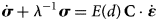
with the elastic modulus tensor ${\bf C}$ (a function of the Poisson ratio ν) and the viscous relaxation timescale λ. Note that the stress and strain rate tensors are reduced in their order by using the Voigt notation for symmetric tensors. The relaxation timescale λ is written as the ratio of the viscosity ξ, the elastic modulus E and a damage parameter d representing the amount material degradation from accumulating micro (sub-grid) cracks in the sea ice (Dansereau and others, Reference Dansereau, Weiss, Saramito and Lattes2016):
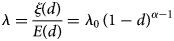
where ξ and E depend on the fractional ice cover, mean ice thickness (i.e. using the formulation for the VP ice strength of Hibler, Reference Hibler III1979) and α > 1 is a parameter ruling the transition from elastic to viscous behaviour. E 0 and ξ 0 are the undamaged mechanical parameters and λ 0 = ξ 0/E 0. In contrast to some previous work (e.g. Dansereau and others, Reference Dansereau, Weiss, Saramito and Lattes2016), we define damage so that d = 0 for undamaged ice and d = 1 for maximally damaged ice.
The damage increases when the stress states exceed the yield curve (Fig. 1) and it contains the history of the previous damaging events (Dansereau and others, Reference Dansereau, Weiss, Saramito and Lattes2016; Plante and others, Reference Plante, Tremblay, Losch and Lemieux2020). The increase depends on the scaling factor d crit (critical damage, which is determined by the requirement to bring the overshooting stress state back to the yield curve).
Illustration of elliptic yield curve (VP, black dotted and solid ellipses) and MC yield curve (MEB, black piecewise linear lines). Invariant stress axes (σ I, σ II) in black and principal stress axes (σ 1, σ 2) in grey. σ c is the critical uniaxial compressive stress (Eqn (3)) and σ t is the critical tensile stress (Eqn (4)). The maximum tensile stress T m (Eqn (6)) is indicated by the green dashed line. a and b denote the semi-major axes of the elliptic yield curve. Grey shading marks the cohesive stress states.
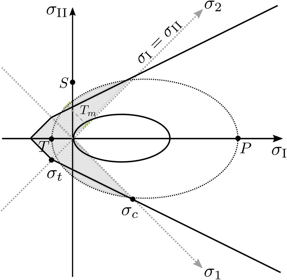
One possible yield curve for the MEB rheology is the MC criterion with a tensile cut-off (Fig. 1) (Dansereau and others, Reference Dansereau, Weiss, Saramito and Lattes2016). The critical uniaxial compressive stress σ c at the intersection of the MC yield curve with the principal stress σ 1 axis (Fig. 1) is

where c is the cohesion and q = ((μ 2 + 1)1/2 + μ)2 is the slope defined by the internal friction coefficient μ. In contrast to the standard elliptic yield curve of a VP rheology (Hibler, Reference Hibler III1979), this yield curve permits isotropic tensile stresses. The critical tensile stress σ t is defined as the intersection of the principal stress σ 2 axis with the MC criterion (Fig. 1) so that

Implementation details
The finite-volume implementation on the C-grid of the MITgcm sea-ice model follows for the most part the implementation of the MEB rheology in the finite-differences C-grid implementation in the McGill sea-ice model (Plante and others, Reference Plante, Tremblay, Losch and Lemieux2020).
We note the structural similarity of the MEB and VP constitutive equations: the product of the elastic modulus tensor ${\it C}$ and the strain rate tensor $\dot {{\bf \varepsilon }}$
 in Eqn (1) is (e.g. Dansereau and others, Reference Dansereau, Weiss, Saramito and Lattes2016)
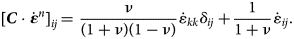
This is the same form as the VP constitutive equation $\sigma _{ij} = 2\eta \dot {\varepsilon }_{ij} + [ ( \zeta -\eta ) \dot {\varepsilon }_{kk} -{P}/{2}] \delta _{ij}$ with P = 0 and shear and bulk viscosities η = (1/2)(1/(1 + ν)) and ζ = (1/2)(1/(1 − ν)). After re-interpreting these variables, we can re-use most of the VP code without additional changes. For details of the discretization we refer to Plante and others (Reference Plante, Tremblay, Losch and Lemieux2020).
On the staggered C-grid, some variables are naturally defined at centre (C) points (e.g. σ 11), while others are naturally defined at corner (Z) points (e.g. σ 12 and $\dot {\varepsilon }_{12}$ ) (Losch and others, Reference Losch, Menemenlis, Campin, Heimbach and Hill2010). Numerical stability requires that σ 12, d crit, d, λ −1 and E are defined on both C- and Z-points of the C-grid cell. The associated averaging is reduced to a minimum, so that only d crit, d, h, a are linearly averaged to Z-points and only $( \dot {\varepsilon }_{12}) ^2$
 is averaged to C-points. E, λ −1 and σ 12 are computed for centre and corner points with the averaged variables.
Validation
We confirmed the plausibility of our MEB implementation with analytic solutions and symmetry tests (not shown, see chs 6 and 7 in Bourgett, Reference Bourgett2022) and with a reproduction of an idealized ice channel (Plante and others, Reference Plante, Tremblay, Losch and Lemieux2020, not shown).
The general behaviour of the dynamics is identical to previous results (Plante and others, Reference Plante, Tremblay, Losch and Lemieux2020). At the beginning of the simulation the tensile stresses downstream of the channel increase and damage develops downstream of each channel boundary. After 3300 s (τ = 0.06 N m−2) a concave shape at the downstream end of the channel indicates the ice arching effect. The stress values agree with the previous results (Plante and others, Reference Plante, Tremblay, Losch and Lemieux2020, their fig. 9). The divergent stress in the middle of the channel is small. The tensile stresses and the shear stresses in the downstream corners of the channel increase so that damage extends over the channel . The ice detaches from the upstream coastline but does not move yet (it remains landfast, land-locked by the islands). Both shear and divergent stress fields downstream of the ice channel drop to zero when the ice downstream of the channel detaches (not shown, see ch. 7 in Bourgett, Reference Bourgett2022).
Comparison of MEB to VP
We can now use the MITgcm model framework to compare small-scale sea-ice deformations with the VP and the MEB rheology using the same grid spacing, discretization and parameters.
For both rheologies the yield curve determines the cohesive strength. The cohesive strength influences the shear deformation of sea ice. If sea ice is driven through a narrow channel the cohesive strength controls the potential for modelled sea ice to form ice arches (Ip, Reference Ip1993; Hibler and others, Reference Hibler, Hutchings and Ip2006; Plante and others, Reference Plante, Tremblay, Losch and Lemieux2020).
For the VP and the MEB rheology, cohesive stress states σ I < |σ II| are marked by grey shading in Figure 1. In terms of the mechanical strength parameters for maximal compression, shear and isotropic tension (P, S, T), the ellipse aspect ratio is defined as e = (P + T)/(2S) with T = kP and the tensile factor k (König Beatty and Holland, Reference König Beatty and Holland2010; Bouchat and Tremblay, Reference Bouchat and Tremblay2017). For the elliptic yield curve, the cohesion increases by decreasing the ratio e of the two semi-major axes (making the ellipse ‘fatter’), by increasing P, and by moving or extending the ellipse into the tensile half-plane (k > 0). Even though the original VP yield curve does not allow isotropic tensile stresses (T = 0 or k = 0, black ellipse in Fig. 1), the tensile strength is not zero. The maximum tensile stress, that is the maximal distance of the yield curve to the diagonal σ I = σ II or maximum of σ 1 (Bouchat and Tremblay, Reference Bouchat and Tremblay2017, and Fig. 1), is defined as
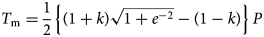
and is non-zero for all k ≥ 0 (Fig. 1).
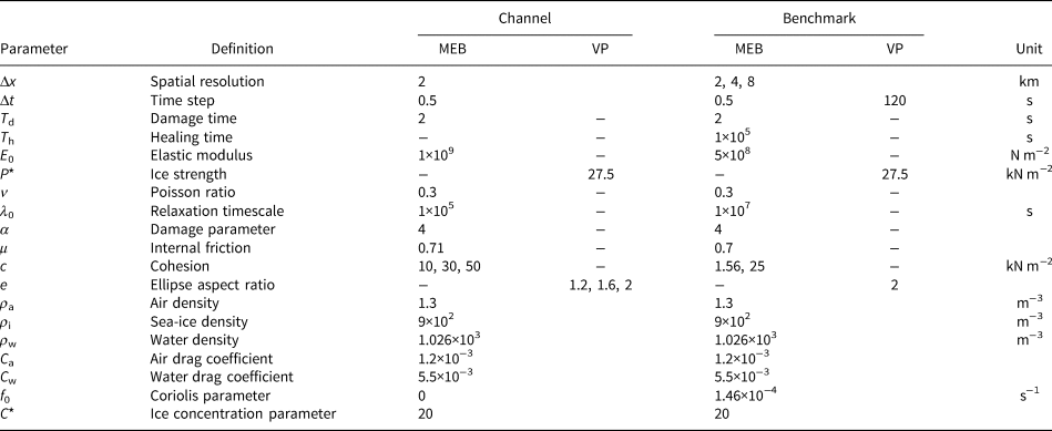
We use an idealized ice channel to tune yield curve parameters of both rheologies to give similar results. Building on this experience, we analyse the effect of gridscale heterogeneity on the solution in a quadratic domain with cyclonic winds (Mehlmann and others, Reference Mehlmann, Danilov, Losch, Lemieux, Hutter, Richter, Blain, Hunke and Korn2021) with similar cohesion for VP and MEB. The VP models uses a JFNK solver that converges with a relative precision of 10−4. All model parameters are summarized in Table 1.
Model parameters of the channel with idealized ice bridge experiment and the quadratic domain with cyclonic winds (‘benchmark’) for the MEB and the VP rheology
Channel with idealized ice bridge
Inspired by previous ice arch simulations (Dumont and others, Reference Dumont, Gratton and Arbetter2009; Dansereau and others, Reference Dansereau, Weiss, Saramito, Lattes and Coche2017), we use an idealized channel set-up modified from Plante and others (Reference Plante, Tremblay, Losch and Lemieux2020). A 800 km × 200 km domain with a grid resolution of 2 km and closed boundaries with a no-slip boundary condition in the x -direction features a channel in the y -direction. The channel itself is 200 km long and 60 km wide. The domain has open boundaries at y = 0 km and y = 800 km with Neumann conditions for all variables. The Neumann conditions ensure that sea ice can drift freely into and out of the domain and does not need to detach from a solid boundary at y = 800 km, so that slowing down of the ice upstream the channel is solely determined by the ice arching. The sea-ice cover is forced by surface stress in the negative y -direction (‘southwards’) that increases linearly from 0 to 0.625 N m−2 within 10 h. The simulation is run for 240 h with no further increase of the forcing. The slowing down of the sea ice upstream of the channel due to the formation of ice arches is used for comparison between VP and MEB.
Different parameters of the yield curves were tested to allow cohesive stress states. We choose the parameters so that the maximum tensile stress T m (Eqn (6)) of the VP rheology is equal to the critical tensile stress σ t (Eqn (4)) of the MEB rheology, since both represent the maximum positive value of the principal stress σ 1 (Fig. 1). Specifically, we choose c = 10 and 30 kN m−2 leading to σ t = 10.4 and 31.24 kN m−1 for MEB. The corresponding T m are computed with P* = 49.92 kN m−2 and P* = 149.92 kN m−2, k = 0.05 and a small value for e = 1.2 (Kubat and others, Reference Kubat, Sayed, Savage and Carrieres2006; Lemieux and others, Reference Lemieux, Dupont, Blain, Roy, Smith and Flato2016).
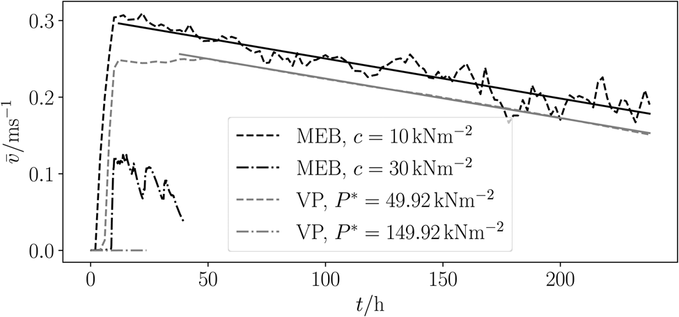
Except for the VP simulations with T m = 31.24 kN m−1, the effect of ice arching to the upstream ice drift velocities can be observed and the ice slows down for both VP and MEB simulation (Fig. 2). The parameter set with T m = 31.24 kN m−1 makes the ice so stiff that it does not start to move at all. The ice drift in the MEB simulation with c = 30 kN m−2 decreases within 40 h. For 10 kN m−2, the ice drift upstream increases quickly and then slows down gradually with rates that are very similar between the MEB (m meb = 1.45 × 10⁻⁷ m s−2) and VP simulations (m vp = 1.43 × 10⁻⁷ m s−2) (Fig. 2, solid lines). Also, the velocity fields upstream (Figs 2, 3) are very similar with c = 10 kN m−2 for MEB and its correspondent mechanical parameters for VP. The maximum ‘southwards’ velocity upstream is reached after approximately 15 h.
Averaged ice velocities parallel to channel upstream of channel. The sea ice does not move at all (VP) or rapidly stops (MEB) for the high cohesion case (c =30 kN m−2, P* =149.92 kN m−2, dash-dotted lines). There is a slow and very similar stopping effect by the formation of an ice arch in both the MEB simulation and the VP simulation for the low cohesion case (c =10 kN m−2, P* =49.92 kN m−2, dashed lines). The solid lines are the linear regression of the ice velocities.
Snapshots of the effective ice thickness h and the ice drift velocity (arrows) for the VP rheology (left two panels) and the MEB rheology (right two panels) at t = 12 and 24 h. Note that the colour scale is chosen to emphasize deviations from the initial state (h =1 m).
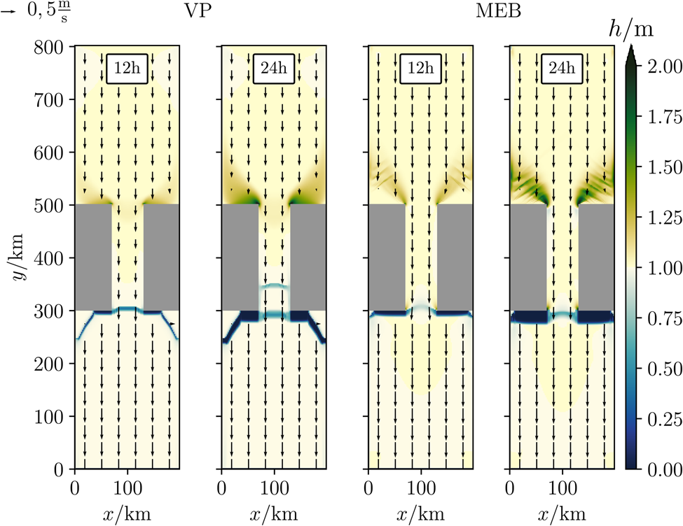
The effective ice thickness is generally similar for both rheologies (Fig. 3). In both cases, leads form downstream of the channel and ridging occurs upstream of the channel. Some differences in the exact location and shape of the leads and ridges are attributed to the different failure processes, namely the damage propagation and the associated normal flow rule for the MEB and VP rheologies, respectively. For instance, some ice remains attached to the islands downstream of the channel in the VP simulation as the deformation transitions from lead opening downstream of the islands to pure shear on the sides, while in the MEB simulation the damage propagation is directly along the coastlines. Upstream of the channel, the ridging area contains additional diagonal patterns in the MEB simulations due to the formation of secondary fracture lines, while the ice thickness is smoother and more uniform in the VP simulations.
Our results agree with other ice arch simulations (Dumont and others, Reference Dumont, Gratton and Arbetter2009; Dansereau and others, Reference Dansereau, Weiss, Saramito, Lattes and Coche2017; Plante, Reference Plante2021, ch. 5) and demonstrate that the cohesive strength of the ice plays an important role in ice arching so that corresponding mechanical parameters lead to similar results between the different rheologies.
Quadratic domain with cyclonic winds
A quadratic box with closed boundaries, constant anticyclonic (clockwise) ocean circulation and a moving cyclonic wind system was suggested to compare different sea-ice models (Mehlmann and others, Reference Mehlmann, Danilov, Losch, Lemieux, Hutter, Richter, Blain, Hunke and Korn2021). This ‘benchmark’ problem was used to analyse how different VP models simulate sea-ice deformation, in particular LKFs. Here, the ‘benchmark’ problem is repeated with the MITgcm using different grid spacings (Δx = 2, 4, 8 km) to analyse spatial heterogeneity in both the MEB and VP models. Note that for all grid resolutions the simulation is produced with the same time step (Δt = 120 s for VP, Δt = 0.5 s for MEB). In the MEB case, this value is chosen to ensure that the constitutive equation is well resolved at the highest resolution (i.e. according to the CFL criterion for resolving the elastic waves).
To choose similar yield curve parameters for MEB and VP as in the channel experiment, we have to consider the following: the VP parameters of this benchmark P* = 27.5 kN/m2 with e = 2 and no tensile stress (k = 0) lead to a very low cohesion of 1.56 kN m2 (Eqn (6)). Using the large P* values implied by the cohesion of the channel experiment in the VP rheology would change the benchmark dramatically from previously published results (Mehlmann and others, Reference Mehlmann, Danilov, Losch, Lemieux, Hutter, Richter, Blain, Hunke and Korn2021), so that to compare the different rheologies we instead adjust the MEB parameters to match the low VP cohesion. The low cohesion of 1.56 kN m2 leads to very low stress states. For comparison, we also use a high value of c = 25 kN m2. These cohesion values cover the range of previously reported values (Dansereau and others, Reference Dansereau, Weiss, Saramito and Lattes2016; Plante and others, Reference Plante, Tremblay, Losch and Lemieux2020). The model parameters for the experiments are summarized in Table 1.
Results from Mehlmann and others (Reference Mehlmann, Danilov, Losch, Lemieux, Hutter, Richter, Blain, Hunke and Korn2021) are reproduced by our VP simulations, with more radial features in the compressive stress field than circular ones and without tensile stress states (Fig. 4). In both models, there are fewer identifiable deformation patterns and the deformation fields also become smoother with decreasing resolution (not shown, see ch. 8 in Bourgett, Reference Bourgett2022).
Snapshot of the stress invariant σ I at t = 2 d and with Δx = 2 km of the VP simulation on the left and the MEB rheology with low (centre) and high (right) cohesion. Positive values mean convergence. Divergent (negative) stress state are only allowed in the MEB model. The size of the stress invariant depends on the choice of the cohesion.
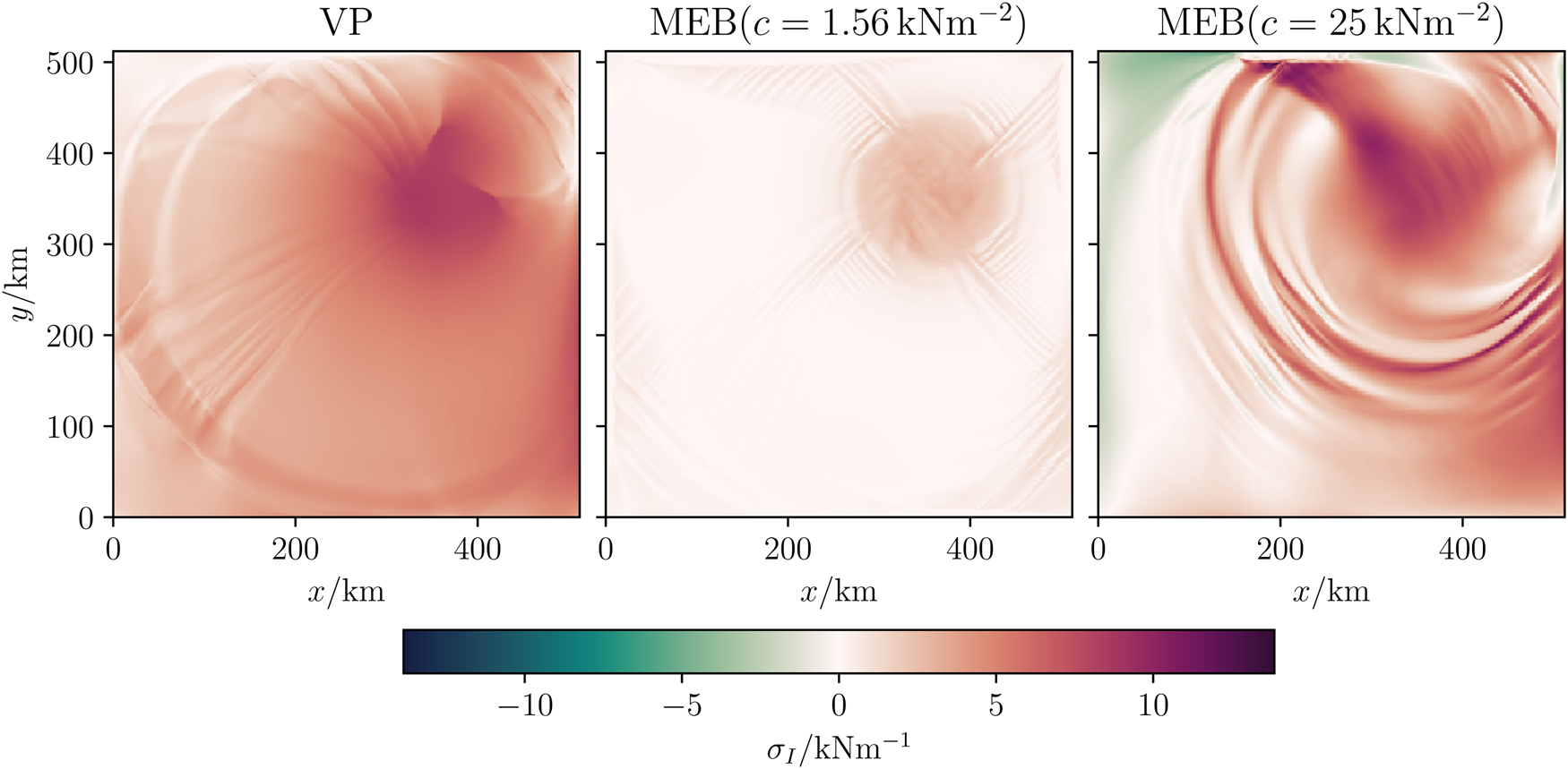
The presence of radial or circular features and the range of the stress values depends to some degree on the choice of cohesion for the MEB rheology. Using the MEB rheology with a cohesion similar to that of the VP simulations yields much smaller stresses but otherwise similar features as in the VP simulations, with mostly radial features and only a few circular stress features. Increasing the cohesion in the MEB model to get similar stress states as in the VP simulation (Fig. 4), however, changes these patterns and the features are mostly circular. Using the VP rheology with analogous values to match the cohesive stress states results in the same dependency (not shown). This dependency suggests that the shape of the features are sensitive to the shear strength; fewer cohesive stress states (grey area in Fig. 1) strongly result in smaller shear stresses, which favours radial features, while more cohesive stress states result in larger shear stresses, which favours the production of circular features.
There are other yield-curve related causes for the different stress fields: for example, the different yield curve shape of the MEB rheology allows isotropic tensile stresses (see negative σ I in Fig. 4), while the VP rheology with the standard elliptical yield curve does not; and the MEB model does not have a flow rule. Neither of these causes are explored here.
Further, the rheologies are compared by means of the number of LKFs as detected by a tracking algorithm (Hutter and Losch, Reference Hutter and Losch2020, with parameter modifications by Mehlmann and others, Reference Mehlmann, Danilov, Losch, Lemieux, Hutter, Richter, Blain, Hunke and Korn2021) (Table 2). The number of LKFs increases for both rheologies with increasing resolution. As expected because of the damage mechanism and long-range elastic interactions that produce sub-grid fracturing (Dansereau and others, Reference Dansereau, Weiss, Saramito and Lattes2016), the MEB simulation (independent of the choice of cohesion) has more LKFs than the VP simulation on all grids, especially on Δx = 2 km grid. Increasing the cohesion tends to lead to fewer LKFs (Table 2). Note that the decreased heterogeneity in the MEB simulations with high cohesion is associated with a much less extensive damage field. As the damage mechanism is known to be a numerical error integrator (Plante and Tremblay, Reference Plante and Tremblay2021), this raises a question about the impact of numerical noise in seeding the heterogeneity.
Number of LKFs for both VP and MEB rheology for simulations with 2 km, 4 km, and 8 km grid spacing Δx
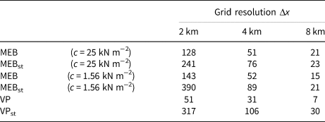
The index ‘st’ indicates that the simulation uses a stochastic parameterization of c (cohesion) for the MEB rheology or P* (ice strength) for the VP rheology. The MEB simulations are run with a high value of c = 25 kN m−2 and with a low value of c = 1.56 kN m−2.
Stochastic parameterization
One of the main motivations to develop a brittle rheology was the observation that models with VP rheology underestimate observed spatial heterogeneity (Girard and others, Reference Girard2011). We indeed found the MEB solution to be more heterogeneous. Alternatively, heterogeneity can be increased with stochastic parameterizations (Juricke and others, Reference Juricke, Lemke, Timmermann and Rackow2013, their fig. 6, and personal communication). In fact, early brittle models used a stochastic cohesion parameter c to introduce disorder (Girard and others, Reference Girard2011; Dansereau and others, Reference Dansereau, Weiss, Saramito, Lattes and Coche2017). We now adopt the same method to account for faults and cracks in the ice below the spatial gridscale Δx and draw the cohesion parameter c from a (pseudo-)random uniform distribution between 0.5c 0 and 1.5c 0 of the unperturbed cohesion c 0. The resulting heterogeneous cohesion field is constant in time throughout the simulation. Because the critical stresses σ c and σ t depend on c (Eqns (3) and (4)), a stochastic cohesion also leads to a different (but constant-in-time) damage criterion for each gridcell.
With the stochastic cohesion the number of LKFs increases for all grid resolutions independent of the cohesion (Table 2). The number of LKFs for the MEB simulations with the stochastic cohesion is also much higher than for the VP simulations discussed above (consistent with Girard and others, Reference Girard2011).
Can we also obtain more spatial heterogeneity with stochastic parameters within the VP model? The VP model does not contain the fast feedback caused by the damage parameter, but the ice strength P* can be perturbed by drawing from the same (pseudo-)random field as the cohesion in the MEB rheology, such that the elliptic yield curve is enlarged or reduced for each gridcell according to P *′ ∈ [0.5P*, 1.5P*]. This choice of P* increases the number of LKFs in all resolutions (Table 2). The LKF numbers are comparable to the corresponding MEB numbers and even higher for lower resolutions.
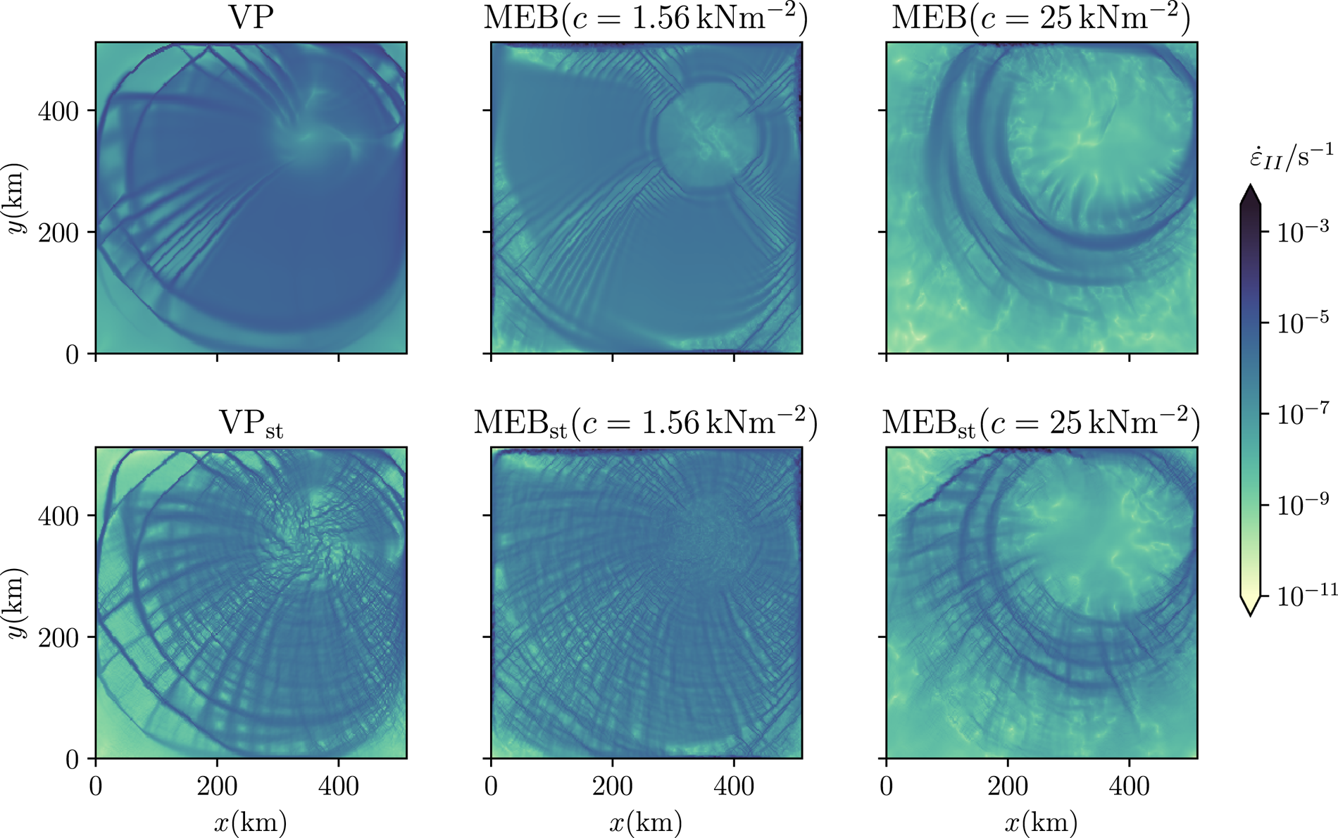
In both rheologies, heterogeneity of the results can be increased by introducing spatial variability to mechanical ice properties (c, P*). The simulations (e.g. shear deformation rate, Fig. 5) contain features of heterogeneity that appear similar to previous results (Girard and others, Reference Girard2011, their fig. 3b). We find (Table 2) that a VP model with a stochastic parameterization can have a similar spatial heterogeneity as the MEB rheology. Note that here a random perturbation of mechanical parameters was similar in both rheologies, whereas Girard and others (Reference Girard2011) compared a standard VP model with smooth ice strength to an EB model with stochastic cohesion. We also note that this random perturbation of cohesion is generally not used in realistic large-scale MEB or BBM simulations with realistic domains (e.g. Rampal and others, Reference Rampal, Bouillon, Ólason and Morlighem2016; Ólason and others, Reference Ólason, Boutin, Korosov, Rampal, Williams, Kimmritz, Dansereau and Samaké2022)
Snapshots of the shear deformation rate $\dot {\varepsilon }_{\rm II}$ at t =2 d and with Δx = 2 km of simulations without (above) and with (below) a stochastic parameterization of the heterogeneity at the gridscale (index ‘st’). The shear deformation rate using the VP rheology on the left and using the MEB rheology with low and high cohesion in the centre and on the right.
Conclusion
Simulations with the MEB rheology tend to be more heterogeneous (i.e. have more LKFs) than simulations with the standard VP rheology. This result was anticipated, but shown here in a controlled environment without confounders. Furthermore, we demonstrate that adding disorder by stochastic mechanical parameters (cohesion for MEB, ice strength for VP) increases heterogeneity to similar levels in the VP and MEB simulations. We conclude that gridscale heterogeneity is one important driver to produce prominent large-scale deformation features, such as LKFs. Gridscale heterogeneity can be introduced in various ways, for example, by a brittle rheology based on physical considerations or by local modification (physical or statistical) of material properties. The latter can be applied to sea-ice models independent of the constitutive equation.
By appropriate choice of model parameters, the most important material property (here, cohesion in a landfast ice simulation in a channel) can be similar between MEB and VP rheologies. This choice leads to similar deformation patterns (Fig. 5, left and middle columns), but the stress states are very different in magnitude between VP and MEB (Fig. 4, left and middle panes). In contrast, tuning the stress states to be of similar order of magnitude (Fig. 4, left and right panes) leads to very different deformation patterns (Fig. 5, left and right columns). In this sense, our results suggest that described differences between deformation patterns can be decreased by tuning the yield curves of the respective rheology.
As a technical note, there is some structural similarity between the constitutive equations for VP and MEB such that after re-interpretation of some variables, a large part of the VP code can be used for the implementation of the MEB rheology (Plante and others, Reference Plante, Tremblay, Losch and Lemieux2020). The time-derivative term, however, increases error memory in the system (Plante and Tremblay, Reference Plante and Tremblay2021). Numerical details, such as averaging between centre and corner points of the C-grid, prove to be crucial for stability of the MEB implementation (see also Brodeau and others, Reference Brodeau, Rampal, Òlason and Dansereau2024). The new damage equation and in particular the elastic wave propagation further pose strict constraints on the time step, so that a time splitting method for the MEB code should be used (Ólason and others, Reference Ólason, Boutin, Korosov, Rampal, Williams, Kimmritz, Dansereau and Samaké2022).
In our simulations, disorder introduced by noise (stochastic parameters) seems to be an important driver of heterogeneity. The VP simulations without additional noise in the ice strength have much fewer LKFs than those with a stochastic strength parameter. The same is true for the MEB simulations but to a smaller extent. The damage parameter in MEB integrates failure by construction, but also numerical errors (Plante and Tremblay, Reference Plante and Tremblay2021). We speculate that these numerical errors may trigger failure and plan to investigate if using a stabilizing scheme for stress correction that minimizes the numerical errors (Plante and Tremblay, Reference Plante and Tremblay2021) will also reduce the simulated heterogeneity.
Acknowledgements
We acknowledge support by the Open Access publication fund of Alfred-Wegener-Institut Helmholtz-Zentrum für Polar- und Meeresforschung. The authors also thank the anonymous reviewers for their constructive comments that helped to improve the quality of the paper.


 Open access