1. Introduction

Antarctic sea-ice dynamics and thermodynamics regulate surface fluxes of heat, water and momentum between atmosphere and the Southern Ocean. Momentum and vorticity is transferred to the ice through kinematic stresses from surface winds. The resulting ice drift arises from a balance between wind stress and a combination of ocean-ice and internal ice stresses, and the Coriolis force. In the Weddell Sea, the circulation pattern comprises a clockwise gyre (Reference DeaconDeacon, 1979). The sea-ice circulation pattern is established by long-term mean synoptic low pressure centered over the eastern Weddell Sea with additional periodic impulses from passing storm systems (Reference Kottmeier and SellmannKottmeier and Sellmann, 1996). Tides and currents provide additional forces, although with different frequencies and a less dominant impact on ice advection (Reference Drinkwater, Tsatsoulis and KwokDrinkwater, 1998b).

During the winter, ice drifts into the Weddell Sea along the northern margin of the Fimbul Ice Shelf in the East Wind Drift (EWD) coastal current. The Antarctic Peninsula impedes westward drift, and ice is compressed before being forced northwards out into the swift-moving eastward Antarctic Circumpolar Current (ACC). The Weddell gyre thus provides a conveyor belt along which fresh water (in the form of ice) and small quantities of brine are transported and redistributed. Continuous ice removal from the southern Weddell Sea results in large polynyas opening along the northern margin of the Filchner-Ronne Ice Shelf. New-ice growth rapidly replaces ice that is advected northwards, yielding enhanced freezing rates over continental-shelf regions. Brine rejected during the freezing process contributes to the salination and nourishment of high-salinity shelf water (Reference Carmack and UntersteinerGarmack, 1986), driving the formation of dense, "deep" and "bottom water" as it sinks and mixes downslope from the continental-shelf break (Reference Warren, Warren and WunschWarren, 1981).

Our knowledge of the Weddell ice-drift dynamics is derived from a combination of historical drifting-buoy deployments since the early 1980s (for detailed reviews see Reference Kottmeier and SellmannKottmeier and Sellmann, 1996; Reference Vihma, Launiainen and UotilaVihma and others, 1996), a drifting ice camp in 1992 (Reference GordonGordon and others, 1993) and assorted model simulations (Reference Lemke, Owens, Hibler and MorrisonLemke and others, 1990; Reference Geiger, Hibler and AckleyGeiger and others, 1998; Reference Harder and FischerHarder and Fischer, 1999). The number of simultaneously reporting buoys in the Weddell Sea has been limited to less than 11, with the maximum of 10 in 1992. Most years are characterized by relatively sparsely distributed satellite-buoy trajectories, preventing a comprehensive picture of the spatial or seasonal-to-interannual variability in ice drift from being established. Early Weddell Sea ice-transport estimates were made by Reference Limbert, Morrison, Sear, Wadhams and RoweLimbert and others (1989) and Reference Vihma, Launiainen and UotilaVihma and others (1996) on the basis of extremely sparse buoy measurements and an empirical relationship between geostrophic wind and ice drift. Each suffers from inaccuracies in the assumed spatial variability of sea-ice thickness and the assumption that ice drift conforms to the linear Reference Thorndike and ColonyThorndike and Colony (1982) model. Model simulations of Weddell Sea ice drift, on the other hand, can be tuned to appear consistent with buoy trajectories (Reference Drinkwater, Fischer, Kreyscher and HarderDrinkwater and others, 1995; Reference Harder and FischerHarder and Fischer, 1999). The resultant ice-thickness distributions have not, however, been rigorously validated against ULS ice-thickness data.

Recently, Reference Harms, Fahrbach and StrassHarms and others (2001) have combined time-series ice-thickness measurements from several upward-looking sonars (ULSs) with buoy-drift results from Reference Kottmeier and SellmannKottmeier and Sellmann (1996) to provide the most detailed picture of time-space variability in ice transport to date. A simple but effective empirical relationship is developed between length of ice season and ULS volume transport. Although this relationship is successfully employed to calculate the interannual variability in the integrated net ice transport, the accuracy of their estimates is limited by the dependence upon an empirical wind-drift factor. Importantly, these data also do not allow seasonal variability in net transport to be calculated.

New Antarctic satellite ice-drift data permit direct ice-transport and −export calculations when combined with direct ice-thickness measurements. In this paper, we take Reference Harms, Fahrbach and StrassHarms and others’ (2001) results a step further towards compiling comprehensive satellite-derived, seasonally varying ice-transport estimates in the Southern Ocean. To accomplish this, we first combine daily satellite measurements of ice drift with daily ULS thickness records to obtain volume transport at each ULS mooring location. A new empirical relationship is then developed between measured ice-thickness and satellite microwave radar image data such that a proxy record of time-space variability in ice thickness can be combined with satellite-derived ice-drift maps. These data are used to calculate monthly mean ice-volume flux across a flux gate linking each ULS mooring location over the period 1992−98.

2. Datasets

ULS ice-thickness measurements

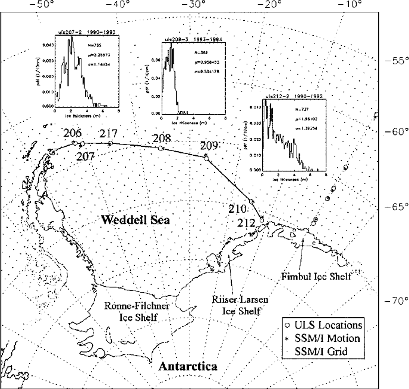
ULS instruments were deployed by the Alfred Wegener Institute (AWI) on 12 bottom moorings spanning the Weddell Sea using the ice-breaker R.V. polarstern (Reference Strass, Fahrbach and JeffriesStrass and Fahrbach, 1998). Figure 1 indicates the locations of each of the moorings together with the conceptual "flux gate" used in our calculations. Mooring sites were chosen to measure the time-varying inflow and outflow of ice in the Weddell gyre. Combined data from multiple mooring deployments span the period 1990−98, although there is no period when ULS operated simultaneously on all moorings. Reference Harms, Fahrbach and StrassHarms and others (2001) describe in further detail all measurement periods for each of the ULS moorings as well as the redeployments.

Fig. 1.

Map of weddell sea moorings deployed by the awiand the flux gate (solid line) across which ice area and volume fluxes are computed. insets show ice-thickness probability distributions from 207−2, 208−3 and 212−2 during the periods indicated. grid-points indicate locations ofeulerian ssm/idrift, and stars indicate gridpoints from which ice-drift velocities are combined with ULS mooring data. moorings along the greenwich meridian are not discussed in this paper.

Each operable ULS instrument recorded the time-varying sea-ice draft di at 8 min intervals over deployment periods of 1−2 years. ULS draft measurement data supplied by the AWI were already binned in two different ranges (0−10 m; and all drafts). Data binned in the cut-off range 0−10 m are used by Reference Harms, Fahrbach and StrassHarms and others (2001) to assess relative iceberg bias to ice-thickness distribution. Both datasets were ensemble-averaged over 24 h and monthly intervals, and ice draft converted to thickness hi using after Reference Harms, Fahrbach and StrassHarms and others (2001). This draft-to-thickness relationship was established from ice-core drillings in the Weddell Sea (Reference Wadhams, Lange and AckleyWadhams and others, 1987; Reference Lange and EickenLange and Eicken, 1991; Reference Eicken, Lange, Hubberten and WadhamsEicken and others, 1994).

3. Satellite Ice Drift

Time-varying Eulerian ice velocity Vi(t) was extracted from the gridded SSM/I motion data at each of the ULS locations and combined with the corresponding ice thickness Hi(t) to compute variations in ice-volume transport. Monthly averaging was performed on both daily datasets prior to the multiplication.

Figure 2 indicates 1994 annual mean daily drift. The colour legend indicates drift speed, and the white streamlines indicate typical trajectories of sea-ice floes in the Weddell gyre. Converging and diverging streamlines intuitively imply ice convergence and divergence. The pattern indicates relatively rapid inflow at Kapp Norvegia focused between ULS 210 and 212, with drift speeds reaching 5 km d⁻¹. Inflowing ice decelerates in the central gyre at its confluence with ice formed along the margin of the Filchner-Ronne Ice Shelves. It is compressed against the coast of the Antarctic Peninsula and forced northwards. Ice drifts parallel to the Peninsula before accelerating and turning northeastwards as it passes Joinville Island and becomes entrained in the ACC. The highest drift speeds are observed in the marginal ice zone, where winds and currents combine to drive the ice at >6 km d⁻¹. Zones of relatively slower ice drift are observed particularly in the coastal southern and western Weddell Sea due to transfer of internal ice stresses over distances of a few hundred kilometers from the shore.

Fig. 2.

Weddell sea 1994 daily mean ssm/i-tracked ice-drift streamlines, and spatial variability in drift s_peed. ULS mooring locations are indicated.

4. ULS Volume Transport

Figure 1 insets show ice-thickness probability distribution functions (PDFs) at three of seven ULSs along the Weddell flux gate. Statistics are provided for the total number of daily mean values together with the overall mean and standard deviation of ice thickness during the given period of ULS operation. As reported by Reference Strass, Fahrbach and JeffriesStrass and Fahrbach (1998), PDFs in the interior region reflect the maximum attainable thermodynamic growth thickness in a predominantly divergent ice pack. The ULS 208 PDF (Fig. 1) reports a mean thickness of 0.96 m and negligible fractions of ridged ice. In contrast, ULSs 207−2 and 212−2 report large fractions of deformed ice caused by dynamical processes such as ridging of thin ice forming in leads and polynyas. Reference Drinkwater and HaasDrinkwater and Haas (1994) report in situ ice-thickness data along a similar flux gate during 1992 Winter Weddell Gyre Study (WWGS’92). These data indicate the same general ice characteristics across the gyre. ULS 212−2 reports particularly deformed ice in the vicinity of Kapp Norvegia, consistent with helicopter-borne laser-altimeter measurements of highly rubbled and ridged ice (Reference DierkingDierking, 1995), and the polarstern becoming beset in compressed ice in that location in 1992 (Reference LemkeLemke, 1994). As ice circulates around the Weddell Sea, thin ice grown in leads openings during wind-driven or tidal ice divergence becomes rafted and ridged. The increase in the mode from 0.2 to 2.0 m, together with the increase in mean ice thickness between the locations of ULS moorings 212−2 and 207−2 (Fig. 1), is attributed to the redistribution of thin ice into the thicker part of the distribution.

Mean satellite-tracked ice-drift velocities are combined with mean ULS thickness at monthly intervals in Figure 3 to compute volume transport of sea ice. The bottom panel shows the local u and v components of ice velocity (VI), and the middle panel shows monthly scalar mean ULS thickness measurements (hi). The upper panel indicates time-varying volume transport Φ, where Φ = (VI) × (hi).

Fig. 3.

Time series at ULS moorings (a) 207 and (b) 208 of monthly mean ice-volume transport (upper panel), derived from combinations of ULS ice thickness (middle panel) and ssm/i tracked ice-drift speed (lower panel).

Results from ULSs 207−2 and 208−3 indicate an ice-volume flux toward the northeast out of the Weddell Sea throughout the winter months, with a local direction which fluctuates around a mean of −60° (positive = clockwise). Summer reversals in flux direction occur periodically at most ULS locations with southwesterly motion noted in February 1992 at ULS 207 (Fig. 3a), and a more extended period of south-southwesterly ice recession at ULS 208 (Fig. 3b) from January to March 1994. Strong seasonal cycles in velocity and ice thickness near to Joinville Island (ULSs 206, 207 and 217) lead to correspondingly large seasonal variations in volume transport between 0 and 0.42 m3 s⁻¹. In contrast, the central gyre exhibits a much smaller range of seasonal variability marked by a relatively gradual increase in ice thickness over the ice-growth season. The smaller mean and variance in ice thickness and velocity in the interior lead to volume transports in the range 0−0.12 m³ s⁻¹ at mooring 208.

Figure 4 shows a comparison of seasonally varying ULS volume transport during the period of greatest overlap in ULS operation. Relative transport is computed in fixed directions of 225° and 17° for net drift into and out of the Weddell Sea, respectively. Flux magnitudes are roughly equivalent at the eastern and western extremes of the flux gate, although ice is imported along a relatively narrow portion of the eastern end of the flux gate between ULSs 210 and 212 in Figure 2. Seasonal variations in the time series of export at ULSs 207 and 217 are mirrored cycles at locations 212 and 210, suggesting that advection and ice transport in the Weddell gyre speeds up and slows down during the winter and spring months.

Fig. 4.

Seasonal variability in ice-volume transport at ULS moorings.

Significant differences between fluxes computed at ULSs 212 and 210 (in Fig. 4) indicate the strong decay in volume fluxes with distance from the coast noted by Reference Strass, Fahrbach and JeffriesStrass and Fahrbach (1998) at Kapp Norvegia. Furthermore, this difference reiterates that satellite-derived ice-motion datasets and models must effectively resolve strong coastal ice fluxes around the Antarctic coast for the fresh-water balance to be correctly computed. Significant discrepancies are noted at the western end of the flux gate, between the results of Reference Harms, Fahrbach and StrassHarms and others (2001) and our findings. The simple linear drift model they employed does not successfully account for the spatial gradient in ice velocity between ULS 207 and Joinville Island, and as a consequence they overestimate the ice-volume flux at mooring 206.

5. Proxy Ice-Thickness Record

Without simultaneous overlapping annual cycles at each of the mooring locations it is impossible to integrate volume transport across the Weddell Sea. Reference Harms, Fahrbach and StrassHarms and others (2001) find an empirical relationship between annual volume-transport ice and the length of ice season, determined from independent SSM/I ice concentrations. Although this provides a record of interannual variations in volume transport, it does not tell us about the significant seasonal variations clearly apparent in the individual monthly records in Figures 3 and 4. This prompted further efforts to find an empirical relationship allowing monthly mean transports to be calculated along the entire flux gate.

Empirical relationship

Figure 5 shows a scatter plot derived from comparisons of monthly mean b pixel values in EScat images with monthly mean ice thickness at each mooring. The scatter indicates a logarithmic relationship between b and (hi). The following curve was fitted to the data using least −squares regression:

(1)

Fig. 5.

Empirical relationship between weddell sea monthly mean ULS ice thickness and ers scatterometer b image pixel values. the curve indicates the exponential relationship equation (1) fitted to the data. the inset shows the histogram of the residual errors (ULS predicted value) and its comparison with a zero mean gaussian error distribution.

where b is the monthly mean gradient in radar scattering coefficient at the ULS location. A correlation coefficient of r = 0.8 suggests that ∼65% of the year-round variance in ice thickness can be explained by the temporal and spatial variability in G-band scatterometer image data. The rougher the ice surface becomes, the less rapidly radar backscatter decays with increasing incidence angle.

An alternative piecewise linear relationship was tested, which requires a priori distinction between deformed and undeformed ice regimes during different seasonal periods. With limited amounts of monthly ULS data available, this strategy is presently difficult to test or validate. Furthermore, since sufficiently reliable ice-classification data are not available for the entire period of interest, this alternative approach was discarded in favour of a more simple one-parameter fit. Future ULS data collection will allow seasonal and spatially varying relationships to be developed.

Thickness-estimate error analysis

Thickness-estimate error is computed as the difference between monthly mean ULS ice thickness and EScat-predicted ice thickness, as . The inset in Figure 5 shows the histogram distribution of these errors in comparison with a Gaussian distribution. The mean error is close to zero, and the standard error in estimating mean ice thickness is 61 cm. This estimate error is large in comparison with the standard deviation of ice thickness σ_hi. (Fig. 1) or the typical standard measurement error of the monthly mean ULS thickness, defined as Typically, ∼5000 independent ULS thickness samples are taken during a 1 month interval. For a typical mean ice thickness of 0−2 m, this translates into a standard ULS measurement error of ±0.03 m. Though the 61 cm standard error in making estimates from EScat b images is relatively large, it represents only 20% of the range of typical monthly mean thickness values (0−3 m in Fig. 1).

Figure 6 shows a comparison between estimated volume transport, calculated using Equation (1) and SSM/I ice motion, and ULS volume transport Φ described in the previous section. Monthly mean data points are broken down by season to indicate whether seasonal ice conditions impact ice-thickness estimation accuracy. Indeed, there is no apparent seasonal bias in transport estimates in either directional component. The standard deviation in volume-transport estimates using EScat-derived proxy thickness and SSM/I ice motion is therefore 0.05 m3 s⁻¹.

Fig. 6.

Comparison of monthly mean estimates of volume transport at each ULS mooring for ice-covered months with ssm/i ice drift, ULS ice-thickness data and escat estimates of ice thickness.

In general, the empirical relationship has its greatest sensitivity at the thin end of the thickness distribution, and the ERS scatterometer is capable of delineating areas of smooth and deformed young ice. Equation (1) slightly underestimates the thickness of perennial and deformed ice. Regional and seasonal partitioning of data points in Figure 5 demonstrate this is due to winter confusion between volume- and rough-surface-scattering ice-floe surfaces, and the fact that undeformed perennial ice with a deep snow cover can produce a scattering signature similar to that of extremely deformed first-year ice. Summer melting, in contrast, reduces such problems in thickness estimation from b images, as it exaggerates the scattering contrast between ridged/rubbled and level ice surfaces. Wet snow and ice surfaces reduce penetration, thereby limiting confusing volume-scattering effects from internal inhomogeneities within the snow and ice.

6. Integrated Volume Flux

Initially we computed annual net ice-volume flux orthogonal to the flux gate by (i) finite-differencing ULS measured monthly mean Φvalues in Figure 4 (between moorings); (ii) performing a time integral on the resulting monthly flux to obtain annual integrated ice-flux values; and (iii) summing integrated fluxes across all line segments along the flux gate. Results are also compared with those obtained by linearly interpolating to 1 m intervals along the flux gate (as performed by Reference Harms, Fahrbach and StrassHarms and others (2001)), but the results did not differ significantly nor warrant the additional computational burden of interpolation.

Our finite-difference results were compared with those of Reference Harms, Fahrbach and StrassHarms and others (2001) in order to assess the improvement when satellite-tracked drift is incorporated in calculations of net volume flux. Their estimates rely upon a combination of the linear ice-drift model of Thorndike and Colony (driven by European Centre for Medium-range Weather Forecasts winds) with the same ULS thickness data. Relatively, their results suggest significantly exaggerated net ice export and import into the Weddell Sea at moorings 206 and 212, perhaps due to strong seasonal and spatial variability in internal ice strength not captured by the simple advective model. Overall, we obtain a 20% smaller integrated volume transport of 64 × 10³ m³ s⁻¹ for the western outflow and a 50% smaller influx of 18 × 10³ m³ s⁻¹ across the narrow eastern coastal inflow. Our net ice-flux budget orthogonal to the flux gate is therefore 46 × 10³ m³ s–1. Since net ice flux from the Weddell Sea was computed by subtracting inflow from the outflow, it appears that the significantly larger Harms and others net transport values partially cancel out one another. The result is that their overall net integrated volume transport is only around 10% greater than our value.

Comparisons were also made with the results of using the 10 m ice-thickness cut-off statistics described in section 2. A significant decrease is noted in the east-west component in volume flux at ULS 206 when the 10 m cut-off is used for its 1996−97 operating period. This suggests that the iceberg flux from the disintegrating Larsen Ice Shelf (Reference Rott, Rack, Nagler and SkvarcaRott and others, 1998) may have significantly biased ice-thickness statistics at this mooring location. In general, however, use of a 10 m ice-thickness cut-off reduces volume flux by only a few per cent, due to icebergs having limited impact over most of the flux gate.

7. Annual Ice-Volume Fluxes

Since the AWI ULS did not operate simultaneously along the Weddell flux gate, proxy EScat ice-thickness data (from section 5) are required to calculate seasonal and interannual variability in Weddell Sea net ice-volume flux. Monthly mean results in Figure 7 indicate the seasonal and interannual variability in net area and volume flux for periods when the flux gate is covered by ice exceeding 15% concentration. Figure 7a shows a 9 year mean ice-area flux of 29 × 10³ m² s⁻¹ from SSM/I ice-drift data (shown as dotted line). Monthly mean thickness estimates from Equation (1) are combined with the area flux to obtain the 6 year mean volume flux of 3 2 × 10³m3^s–1 (limited to the 1992−98 operation of ERS-1 and −2). This translates to an effective net mean fresh-water export of 32 × 10³ m³ s⁻¹ or 0.032 Sv (1 Sv = 1×10⁶ m³ s⁻¹). To assess errors in computing net fluxes we considered the standard estimation errors for ice drift and thickness in section 2, together with the 1 σerror bound of 0.05 m³ s⁻¹ in transport in Figure 6. We obtain errors in integrated net volume flux of about 25% of the mean monthly flux, and of the order of 5 × 10³ m³ s⁻¹ for the annual means shown in Table 1.

Fig. 7.

Weddell sea monthly mean values of (a) net area flux and (b) net volume flux. horizontal bars in (b) indicate annual means from this study, and solid circles indicate the annual means of Reference Harms, Fahrbach and Strassharms and others (2001). the dashed line in (b) shows the effective ice-thickness multiplier.

Table 1.

Weddell sea annual mean fluxes of ice area and volume from combined ssm/i ice-drift velocities and escat ice-thickness estimates

8. Conclusions

Results in this paper are derived by applying an ice-volume transport integration strategy similar to that of Reference Harms, Fahrbach and StrassHarms and others (2001). Our data indicate that strong spatial gradients in the area flux have a significant impact upon net ice-volume flux, as do strong seasonal-to-interannual fluctuations in ice advection and thickness. Results demonstrate that it is vital to consider both spatial and temporal variability in ice drift in order to capture the true seasonal variance in sea-ice transport or fresh-water flux. It is particularly timely to exploit new gridded satellite-derived ice-drift datasets for this purpose.

As previous results have demonstrated, ice export is greatest at the north-western end of the flux gate (near the tip of the Antarctic Peninsula) and declines eastwards towards the central gyre. Ice import takes place in the coastal current entering at the east of the Weddell Sea across a narrow portion of the flux gate. Individual ULS moorings near Kapp Norvegia can indicate transports of comparable magnitude to those of ULS near the tip of the Antarctic Peninsula. Periods of significant volume import appear closely related to the amount of deformed ice entering along the coastal regime in the eastern Weddell Sea. The occurrence of large seasonal peaks in ice transport at ULS 212, for instance, appears to be related to strong ice-convergence events as reported by Reference LemkeLemke (1994). The net sea-ice budget of the Weddell Sea is, as a consequence, strongly modulated by the quantity of deformed ice carried into the basin along the Coats Land coast.

Direct flux estimates presented in section 7 should be treated with care. It was necessary to assume negligible interannual flux variability in order to combine non-overlapping ULS data from all moorings. We now know this not to be an appropriate assumption. An identical methodology to that of Reference Harms, Fahrbach and StrassHarms and others (2001) was applied simply to make possible direct comparisons between net fluxes with and without satellite ice-drift data. ULS thickness data used in this integration were obtained from mixed periods between 1991 and 1997. Data from ULSs 207, 217 and 212 from the period 1991−92 (Fig. 4), in particular, indicate years and seasons with anomalously large transports. The resulting integrated net flux of 46 × 10³ m³ s_–1 is therefore biased high relative to the estimated 6 year mean of 32 × 10³ m³ s –1

Interannual variations in area and volume flux appear to indicate multi-year cycles characterized by positive and negative anomalies with wavelengths of several years. This is not surprising given other supporting evidence for anomalies in sea-level pressure and large-scale atmospheric circulation patterns (Reference DrinkwaterDrinkwater, 1997). The time-scales associated with resulting patterns of fresh-water depletion and salt enrichment make it imperative that continued systematic, long-term in situ observations are made of ocean and ice properties in this region. This requires carefully designed deployments of moored sensors such as the AWI ULS data exploited in this study. The demonstrated relationship between ice-thickness and satellite data is undoubtedly limited by the highly variable regional and seasonal characteristics of Weddell Sea ice. Future calculations of net ice-volume flux will require continued seasonal-to-interannual measurements from such moored ULS sensors such that an accurate satellite-derived proxy record for ice thickness can be suitably developed. Only then can detailed satellite- derived ice-drift data and thickness estimates be fully exploited for Southern Ocean-wide fresh-water and salt-balance calculations.

In future extensions of this work, we plan to compute fluxes using SSM/ I gridpoint measurements of ice velocity at 100 km intervals along the flux gate, rather than finite-differencing between ULS mooring locations. This additional information on the spatial variability in ice drift and thickness will undoubtedly change the preliminary results shown here. Such data will allow much more accurate Weddell Sea budget estimates for salt and fresh water than could previously be made with sparsely deployed buoy arrays.