2. Numerical model and test cases

The numerical model (Chang, Constantinescu & Park Reference Chang, Constantinescu and Park2007) solves the incompressible Navier–Stokes equations and uses detached eddy simulation (DES) to account for the effect of the unresolved scales on the resolved energetically important eddies in the flow. The Spalart-Allmaras model that solves a transport equation for the modified eddy viscosity, $\tilde{\nu }$, is used as the base RANS model. As customary in DES, the turbulence length scale is redefined away from the solid surfaces, where it becomes proportional to the cell size, similar to classical large eddy simulation. The standard value of the model constant (C_DES = 0.65) was used to control the switch from RANS mode to LES mode. The simulations were performed using the Delayed version of DES (Spalart Reference Spalart2009) that preserves the RANS mode inside the attached boundary layers. The governing equations are transformed to generalized curvilinear coordinates on a non-staggered grid and integrated in time using a fully implicit fractional-step method. The convective terms in the momentum equations are discretized using a blend of fifth-order accurate upwind-biased scheme and second-order central scheme. The second-order upwind scheme is used to discretize the convective terms in the equation solved for $\tilde{\nu }$. At the solid boundaries, $\; \tilde{\nu }$ is set equal to zero. All other terms in the governing equations are discretized using second-order central differences. The discrete momentum (predictor step) and turbulence model equations are integrated in pseudo-time using an alternate-direction-implicit approximate factorization scheme.

The numerical model was extensively validated based on comparison with experimental data and data from well-resolved LES. Such validation studies include flow past isolated surface-mounted circular and rectangular cylinders as well as flow past rectangular obstructions placed at one side of an open channel (Koken & Constantinescu Reference Koken and Constantinescu2009; Kirkil & Constantinescu Reference Kirkil and Constantinescu2015). The numerical model was found to accurately predict the mean flow and turbulence statistics inside the wake region and the horseshoe vortex system forming around the front face of the surface-mounted obstruction. The numerical model was also found to accurately predict the spatial development of shallow mixing layers forming in open-channel flows and the characteristics of the mixing layer vortices (e.g. size, shape, non-dimensional passage frequency) over the initial regime and over the quasi-equilibrium regime where the mixing layer undergoes stabilization due to the effect of bed friction on the mixing layer vortices (Cheng & Constantinescu Reference Cheng and Constantinescu2020). Directly relevant for the present investigation, the numerical model was validated for flow past an emerged circular array of solid cylinders by Chang et al. (Reference Chang, Constantinescu and Tsai2017) using the experimental data of Zong & Nepf (Reference Zong and Nepf2011).

The computational domain is shown in figure 1. The present numerical study considers rectangular arrays with $L/W \gg 1$ and $L/D \gg 1$ corresponding to a long rectangular porous region with moderately shallow flow conditions. The values of the main variables in the simulations are summarized in table 1. Simulations were performed with varying ϕ, aW, d/D and cylinder cross-section (circular and square) but with constant W/D. The bed is located at z = 0 and the free surface at z = D. The origin of the system of coordinates is located at the inlet section (x/D = 0) such that y/D = 0 at the sidewall containing the array. The width of the open channel is 4.8D, the channel length is 59D and the array starts at x/D = 8. The length of the array is L/D = 33–35, its width is W/D = 1.6 and the channel Reynolds number defined with the mean incoming flow velocity U is Re_D = UD/ν ≈ 12 000, whereν is the kinematic viscosity. The solid cylinder Reynolds number, Re_d = Ud/ν is larger than the threshold value (Re_d ≈ 120) required for generation of vortex shedding in the wakes of the cylinders situated close to the front and lateral faces of the array. The solid cylinders forming the array were placed using a close-to-regular staggered pattern in the x–y planes, using the randomization procedure employed by Chang & Constantinescu (Reference Chang and Constantinescu2015) and Chang et al. (Reference Chang, Constantinescu and Tsai2017) to reduce the regularity of the wake-to-cylinder interactions. A random displacement of 0.05D–0.1D was applied to the horizontal position of the solid cylinders on top of the regular staggered pattern. Moreover, such an arrangement is closer to that of the plant stems inside patches of natural vegetation (Maza et al. Reference Maza, Lara and Losada2015).

Table 1.

Main geometrical and flow variables of the test cases (ϕ is the solid volume fraction of the array, SC refers to a simulation conducted with square cylinders, N is the number of cylinders in the array, d is diameter/width of the circular/square cylinders, D is the flow depth, W is the width array, L is the length of the array, Re_D = UD/ν, Re_d = Ud/ν, a is the frontal area per unit volume for the array, St_SL is the Strouhal number defined with U and D corresponding to the most energetic frequency in the downstream part of the shear layer, St_array is the Strouhal number corresponding to the wave-like oscillations of the streamwise velocity inside the downstream part of the array, λ is the wavelength of the shear layer vortices in the downstream part of the shear layer, U ₁ and U ₂ are the mean streamwise velocities in the inner-layer region inside the array and in the free stream, outside of the shear layer, respectively, at streamwise locations where the shear layer width is close to constant, L_s is the distance from the back of the array where the flow separates, L_sep is the length over which recirculation bubbles are present in the wake of the array).

The solid volume fraction is defined as the ratio between the total volume of the N solid cylinders forming the array and the volume of the array. In the case of circular cylinders, $\phi = N{\rm \pi} {d^2}/4(WL)$, while for rectangular cylinders $\phi = N{d^2}/(WL)$. In the present study, the solid volume fraction, ϕ, is varied between 0.02 and 0.1 mainly by increasing the number of cylinders per unit area. The paper discusses cases with ϕ < 0.1, which is the range expected for patches of vegetations growing on floodplains and wetlands. For example, for marsh emerged grasses 0.001 < ϕ < 0.02, while for most vegetation growing in rivers 0.05 < ϕ < 0.1 (Leonard & Luther Reference Leonard and Luther1995; Ciraolo, Ferreri & LaLoggia Reference Ciraolo, Ferreri and LaLoggia2006; Zong & Nepf 2010, Reference Zong and Nepf2011). The corresponding range for the non-dimensional frontal area in the present simulations is 0.255 < aD < 1.02, where $aD = N(d/D)/(WL/{D^2})$. The ranges for ad and aW are 0.026 < ad < 0.102 and 0.408 < aW < 1.6. The total drag force acting on the array is expected to scale with 1/a. The other relevant (non-dimensional) length scale is d/W. The main characteristics of the mean flow and turbulence inside the array (e.g. the wake-to-cylinder interactions) are expected to depend mainly on ϕ. To illustrate the separate effects of these two main parameters characterizing the density of the array region, the matrix of simulations in table 1 considers cases with same aW but with different ϕ and also cases with same ϕ but with different aW.

In the present simulations, the horizontal mesh contained close to 1.5 million cells and 48 points were used to resolve the flow in the vertical direction. The mesh was refined inside the array and in the region containing the horizontal shear layer. In the vertical direction, the mesh was refined close to the channel bed where the first point off the bed was situated at 0.0015D. The same wall normal grid spacing was used near the channel sidewalls. In non-dimensional wall units (Re_D ≈ 12 000), the first point off the smooth channel bed and the smooth sidewalls was situated at approximately one wall unit and at least two points were placed inside the viscous sublayer such that the use of wall functions was avoided. Close to the free surface, the vertical grid spacing was close to 0.027D. The average grid spacing in the horizontal direction inside the array was close to 0.017D away from the surface of the solid cylinders. Close to the surface of the cylinders, the wall normal grid spacing was close to 0.0025D (= 0.025d for d/D = 1). Close to 32 grid points were placed on the circumference of each solid cylinder. When expressed in non-dimensional wall units, the average size of the cells inside the array and the shear layer regions in the present simulations were finer than those in the circular array simulations (Re = 67 000) discussed by Chang et al. (Reference Chang, Constantinescu and Tsai2017, Reference Chang, Constantinescu and Tsai2020). The same studies discuss the minimum mesh density needed to obtain grid independent solutions. These findings were used when meshing the computational domain in the rectangular array simulations discussed in the present paper. Additionally, a simulation was run for an isolated long circular cylinder at Re_d = 480, which is representative of the physical Reynolds number for the cylinders situated away from the front face of the array. The horizontal mesh resolution around the cylinder and the wall normal grid spacing near its surface were similar to the ones used for the cylinders forming the array region. The predicted mean streamwise drag coefficient was 1.22, which is close to the value (1.2) inferred from experiments (Munson et al. Reference Munson, Okiishi, Huebsch and Rothmayer2012). The predicted wake shedding Strouhal number defined with the diameter of the cylinder and the incoming velocity was 0.208, very close to the experimental value (≈0.21) reported at similar cylinder Reynolds numbers (Zdravkovich Reference Zdravkovich1997).

The set-up of the present numerical simulations and ranges of the main non-dimensional variables are similar but not identical to those in the experiments reported by White & Nepf (Reference White and Nepf2007) and Zong & Nepf (Reference Zong and Nepf2011) that were conducted with circular cylinders of smaller diameter. The parameters of the numerical test cases were chosen such that the simulations can be conducted with reasonably high computational resources while being able to investigate the changes in the flow as only one of the main non-dimensional parameters was varied (e.g. effect of varying ϕ while keeping aD and aW constant, effect of varying aD and aW while keeping ϕ constant, effect of the shape of the cylinders while keeping aW and aD constant). In particular, the range used for the solid volume fraction (0.02 < ϕ < 0.1) and the ratio between the width of the patch and the width of the channel were the same in the present numerical study and the aforementioned experiments. The experimental ranges of ad (0.024 < ad < 0.12) and Re_D (6000 < Re_D < 28 000) were quite close to those of the present simulations (table 1). Given the smaller values of d/D and W/D in the experiments (0.046 < d/D < 0.1, 3 < W/D < 6.6) compared to the present simulations (0.1 < d/D < 0.2, W/D = 1.6), larger differences are observed for the ranges of aW and aD between experiments (1.6 < aW < 8.4, 0.52 < aD < 2.8) and simulations (0.408 < aW < 1.6, 0.255 < aD < 1.02).

As for previous applications of this code to predict flow in open channels containing arrays of cylinders (Chang et al. Reference Chang, Constantinescu and Tsai2017, Reference Chang, Constantinescu and Tsai2020), the velocity fields at the inflow section were obtained from precursor simulations performed in a straight channel (height 1D, length 16D, width 4.8D) with periodic boundary conditions in the streamwise direction. The free surface was modelled as a shear-free rigid lid with zero vertical velocity. A convective boundary condition was used at the outlet section of the domain containing the array. The channel bed, the sidewalls and the surfaces of the solid cylinders were treated as no-slip smooth walls. The time step (Δt = 0.001D/U) was sufficiently low to resolve the energetic frequencies associated with vortex shedding in the wake of the solid cylinders (e.g. one shedding cycle was resolved with close to 500 time steps for the cylinders that are shedding) and with the formation of vortical eddies inside the upstream part of the horizontal shear layer. Preliminary simulations showed that a distance of 8D between inlet boundary and the front face of the array was sufficient for the adverse pressure gradients generated by arrays with ϕ ≤ 0.1 to become negligible close to the inflow section. Mean-flow and turbulence statistics were collected over a time interval of about 200D/U.

The findings of the present study should be interpreted with care before being used to make predictions for flow in natural channels containing long patches of vegetation at one of their banks. Similar to laboratory investigations of the same flows, the incoming flow was turbulent, but the channel Reynolds number was much smaller compared to typical field Reynolds numbers in rivers. The same was true for the cylinder Reynolds number, which obviously induces some differences in the eddy content and turbulence characteristics inside and outside the array. Simulations were conducted in a straight channel with a horizontal, smooth bed, while in the field the channel bed is deformed and the bed is rough. The plant stems were modelled as rigid cylinders, so the plant flexibility and the associated two-way coupling between the flow and the vegetation were ignored. The cylinders were close to uniformly distributed inside the array and of constant diameter, while in natural patches of vegetation the solid volume fraction of the vegetated patch presents some level on non-uniformity and the diameters of the plant stems are not constant.

Still, this simplified geometrical set-up can be used to provide a fundamental understanding of the dynamics and structure of the shear layer forming at the interface between an elongated patch of vegetation and the free-stream region for cases when the lateral face of the patch is approximatively aligned with the main flow direction in the channel. The formation of a downflow which induces strong 3-D effects around and inside the upstream part of the array is also a general feature of flows past finite-size patches of vegetation in natural channels where the large-scale structures generated by the downflow (e.g. near-bed region of flow acceleration, horseshoe vortices around the upstream face of the patch or around the base of the plant stems directly exposed to the flow) drive the local scour developing next to and inside the front part of the vegetation patch. Moreover, this simplified set-up can be used as a canonical case with respect to which additional relevant effects can be investigated (e.g. plant stem flexibility, non-uniformity of the solid volume fraction inside the array, shape of the front side of the array). The present configuration also serves as a limiting case for studying flow past submerged patches of vegetation located at the side of an open channel where a shear layer flow develops not only at the lateral face of the patch but also over its top face.

3. Comparison with experimental data

Simulation results show that the shear layer development is qualitatively similar to that observed experimentally by White & Nepf (Reference White and Nepf2007). For all simulations, an initial region is present where the shear layer vortices penetrate more inside the array with increasing distance from the leading edge (e.g. see discussion of figure 5). White & Nepf (Reference White and Nepf2007) have shown that the constraint imposed by the finite width and depth of the channel in which the shear layer develops, leads to a clear reduction of the rate of growth of the shear layer width on the free-stream side and to a close to constant lateral penetration width of the shear layer vortices on the array side at large distances from the shear layer origin. Such an evolution toward a constant-width shear layer is similar to that in a classical shallow mixing layer (Sukhodolova & Sukhodolov Reference Sukhodolova and Sukhodolov2012a; Constantinescu Reference Constantinescu2014).

Once stabilization effects become important, the inflection point in the velocity profile situated at y = y_o (figure 1b) moves very close to the lateral face of the array (y = W = 1.6D). White & Nepf (Reference White and Nepf2007) have shown that the shear layer velocity profile is asymmetric and has a two-layer structure. The outer region on the free-stream side resembles a boundary layer, while the inner region of the shear layer contains a velocity inflection point. The maximum Reynolds stress, $- {(\overline {u^{\prime}v^{\prime}} )_{max}}$, occurs at y = y₀ over the downstream part of the shear layer. In a good approximation, the interfacial shear stress can be estimated as $u_\ast ^2 ={-} {(\overline {u^{\prime}v^{\prime}} )_{max}}$. The length scale for the penetration of the shear layer vortices δ_I can be calculated as the distance from the inflection point where the mean streamwise inside the array becomes close to constant ($\bar{u}(\kern-0.5pt y) = {U_1}$, where U ₁ is the inner-layer mean velocity) in the transverse direction (figure 1b). This distance can be estimated by fitting a hyperbolic tangent profile to the simulated/measured profile in the y < y_o region (Raupach et al. Reference Raupach, Finnigan and Brunnet1996; White & Nepf Reference White and Nepf2007). For the outer region, White & Nepf (Reference White and Nepf2007) proposed a boundary layer analogy to scale the velocity profile. They have shown that the width of the outer region, δ₀, is proportional to the ratio between the flow depth, D, and the bed friction coefficient. They defined an effective boundary layer origin (y = y_m where $\bar{u}({y_m}) = {U_m}$, figure 1b) as the lateral distance at which the inner- and outer-layer slopes of the velocity profiles match. The outer-layer length scale defines the distance away from the patch where $\bar{u}(\kern-0.5pt y)$ approaches the mean free-stream velocity outside the shear layer, U ₂. Following White & Nepf (Reference White and Nepf2007), this length scale is estimated as ${\delta _o} = ({U_2} - {U_m})/{(\textrm{d}\bar{u}/\textrm{d}y)_{y = ym}}$. In principle, the inner and outer-layer variables should be calculated using the depth-averaged velocity profiles that are readily available from simulations. However, to allow a more direct comparison with the experiments of White & Nepf (Reference White and Nepf2007), the predicted non-dimensional velocity and Reynolds shear stress profiles at mid-flow depth (z = D/2) were plotted in figures 2 and 3 for the simulations conducted with circular cylinders of constant diameter (d/D = 0.1).

Figure 2.

Non-dimensional spanwise profiles of the mean streamwise velocity at z = D/2 and x = 37.5D in the simulations with 0.02 < ϕ < 0.08 and circular cylinders (d/D = 0.1). (a) Inner-layer scaling; (b) outer-layer scaling. Also shown are the experimental data (cases 1 to 11) from the experiments of White & Nepf (Reference White and Nepf2007) conducted with 0.02 < ϕ < 0.1 and 0.09 < d/D < 0.22.

Figure 3.

Non-dimensional spanwise profiles of the primary shear Reynolds stress at z = D/2 and x = 37.5D in the simulations with 0.02 < ϕ < 0.08 and circular cylinders (d/D = 0.1). (a) Inner-layer scaling; (b) outer-layer scaling. Also shown are sample data from the experiments of White & Nepf (Reference White and Nepf2007) conducted with 0.02 < ϕ < 0.1 and 0.09 < d/D < 0.22.

Figure 2 compares the predicted non-dimensional mean velocity profiles at x/D = 37.5, where simulation results show that the rate of growth of the shear layer width is close to zero (ϕ ≥ 0.04) or relatively small (ϕ = 0.02). Also plotted are the measured profiles from the experiments of White & Nepf (Reference White and Nepf2007) conducted with 0.02 < ϕ < 0.1 and 0.09 < d/D < 0.22. Despite some differences in the geometrical variables defining the array in the simulations and experiments, the level of agreement is good. Inside the inner layer (figure 2a), the predicted profiles of the rescaled velocity $(\bar{u} - {U_1})/2{U_s}$ versus the inner-layer coordinate, $(\kern-0.5pt y - {y_o})/{d_I}$, show very good agreement with the experimental measurements, where ${U_s} = U({y_o}) - {U_1}$. Inside the free-stream region, both simulations and experiments predict a decrease of the rate of growth of the rescaled velocity with increasing ϕ, but the effect is larger in the experiments. Inside the outer layer, the predicted profiles of the rescaled velocity $(\bar{u} - {U_m})/({U_2} - {U_m})$ versus the outer-layer coordinate, $(\kern-0.5pt y - {y_m})/{d_o}$, are in good agreement with the measured profiles. The best agreement is observed for ϕ = 0.08.

Similar to the approach used for the mean streamwise velocity profiles, figure 3 shows the normalized Reynolds stress profiles, $(\overline {u^{\prime}v^{\prime}} )/u_\ast ^2$, in inner- and outer-layer coordinates. Simulation results show that the absolute maximum occurs very close to the extremity of the array. As discussed later, this peak is induced by eddies shed in the wakes of the cylinders situated at the interface with the free-stream region. A second smaller peak is observed on the free-stream side. This peak is mainly associated with the advection of shear layer vortices. Its distance from the interface increases from $(\kern-0.5pt y - {y_m})/{d_o} = 0.4$ for $\phi = 0.08$ to $(\kern-0.5pt y - {y_m})/{d_o} = 0.6$ for $\phi = 0.02$, which is consistent with the increase in the size (e.g. width) of the shear layer vortices with decreasing ϕ (see also discussion of figure 5). The second peak is also observed in several of the experimentally measured profiles (figure 3).

4. Effect of array characteristics on flow and turbulence inside and around the array

4.1. Flow structure inside the array and near the interface with the open flow region

Due to the diversion of the flow approaching the front face of the array, the flow inside the array close to its upstream corner has a strong transverse component away from the channel sidewall. The direction of the flow inside the array can be inferred from the orientation of the wakes and the 2-D streamline patterns shown in figure 4. As a result, a significant part of the flow entering the array at its front face leaves the array through the upstream part of its lateral face. The eddies shed in the wakes of the cylinders close to the lateral interface and the upstream corner of the array delay the formation of the shear layer vortices.

Figure 4.

Vertical vorticity, ${\omega _z}(D/U)$, in the z/D = 0.9 plane. (a) ϕ = 0.08, aW = 1.63, d/D = 0.1; (b) ϕ = 0.02, aW = 0.408, d/D = 0.1. The (ai) and (bi) panels show the instantaneous streamwise velocity, u/U, along a line cutting through the middle of the array (y/W = 0.5 or y/D = 0.8, z/D = 0.9). The (aii) and (bii) panels show the instantaneous flow vorticity distribution close to the front of the array (see insets in panels (a,b)). The (aiii) and (biii) panels show the mean-flow vorticity distribution and streamline patterns close to the front of the array. The red arrows point toward eddies generated in the wake of the cylinders situated near the lateral face of the array that penetrate way inside the free-flow region. The black arrows point toward regions of lower streamwise velocity associated with the wave-like oscillations generated inside the downstream part of the array and downstream of it.

Similar to circular arrays (Chang & Constantinescu Reference Chang and Constantinescu2015; Chang et al. Reference Chang, Constantinescu and Tsai2017), most of the flow entering the array at its front face is diverted laterally (e.g. see 2-D streamline patterns in figure 4). This means that the mechanism responsible for the decay of the bleeding flow at the back of the array with increasing ϕ or aW is the same despite the different shape of the array. In the case of the present rectangular array, the length of the diverging flow region is approximately 3.5D (8 < x/D < 11.5) in the aW ≈ 1.6 (ϕ = 0.08, d/D = 0.1) cases with circular cylinders (figure 4a) and square cylinders. Analysis of the distributions of the mean, depth-averaged transverse velocity at the lateral face of the array for these two simulations shows that approximately 50 % of the flow (e.g. streamwise discharge) entering the array through the front face leaves the array through the first 3.5D of its lateral face. However, the mean flow near the lateral face continues to have a transverse component oriented toward the free-flow region downstream of the diverging flow region (see 2-D streamline patterns in figure 4a). Another close to 30 % of the flow entering the front face of the array will leave the array through its lateral face until the mean streamwise discharge inside the array becomes close to constant (see discussion of figure 6). A diverging flow region is hardly observable in the aW = 0.408 (ϕ = 0.02, d/D = 0.1) case (figure 4b), where the wakes of the cylinders situated close to the front of the array are fairly well aligned with the streamwise direction. However, the predicted mean, depth-averaged velocity field shows that the flow leaves the array through its lateral face over the whole length of the array, with only approximately 20 % of the flow entering the front of the array leaving it over the first 3.5D of the lateral face. Moreover, the mean, depth-averaged transverse velocity at the lateral face decreases monotonically with increasing x/D over the whole length of the lateral face. For the cases with aW > 0.8, the array is sufficiently long such that one can consider that the mean, depth-averaged transverse velocity at the lateral face is negligible over some distance from the back of the array. This is the region over which the streamwise flow discharge inside the array is constant.

The interaction of the shear layer vortices with the cylinders situated close to the lateral face of the array results in the entrainment of energetic vortical eddies from the wakes of these cylinders into the free-stream region of the channel. Some of these eddies penetrate deep (e.g. more than 1.5D) inside the free-stream region (see red arrows in figure 4). Another very interesting phenomenon is present in the instantaneous flow fields. For all cases, successive regions of high and low vertical vorticity magnitude are present inside the downstream half of the array (e.g. see figure 4a). Analysis of the velocity fields shows that the formation of these regions is due to the generation of wave-like, large-scale oscillations of the instantaneous streamwise velocity inside the array (e.g. starting at x/D ≈ 27 in the ϕ = 0.08, aW = 1.63 case and at x/D ≈ 34 in the ϕ = 0.02, aW = 0.408 case, see panels (ai) and (bi) in figure 4). These oscillations are also observed downstream of the array. For all cases, the mean average distance between successive regions of low streamwise velocity, λ_LV/D, is close to the average wavelength of the shear layer vortices, λ/D, given in table 1. For same shape and diameter of the cylinders, the non-dimensional frequency associated with the wave-like oscillations, St_array = fU/D, increases with increasing aW while λ_LV/D decreases with increasing aW. For constant aW, increasing the degree of bluntness of the cylinders (e.g. using square cylinders instead of circular cylinders that for the same width/diameter induce stronger adverse pressure gradients away from their front face) results in larger values of St_array. For constant aW and same shape of the cylinders forming the array, St_array increases with increasing cylinder width-to-depth ratio, d/D (table 1).

4.2. Shear layer vortices

In all simulations, small vortex tubes start forming inside the horizontal shear layer approximately 3D–4D from the front face of the array. These vortex tubes grow mostly via vortex pairing into well-defined shear layer vortices. While in the cases with a large aW (figure 5a,b) the vortex tubes develop over a fairly small streamwise distance from the front face of the array (e.g. 4D–6D from x = 8D for aW ≈ 1.6) into large shear layer vortices, in the cases with a small aW the first shear layer vortices develop at larger distances from the front face of the array (e.g. 16D–18D from x = 8D for aW = 0.408, figure 5c). Over the downstream part of the array, the size of these vortices is increasing with decreasing aW (figure 5b,c) and decreasing degree of bluntness of the cylinders forming the array (figure 5a,b). Over the last 16D of the array length, the wavelength to width ratio of the shear layer vortices decreases from approximately 3.75 for aW = 0.408 to 2.9–3.2 for the two simulations with aW ≈ 1.6. These values are fairly close to a ratio of 3.0 expected for vortices in free shear layers (Browand & Weidman Reference Browand and Weidman1976).

Figure 5.

Instantaneous flow 2-D streamline patterns in the z/D = 0.9 plane in a frame of reference moving with the mean velocity of the shear layer vortices. (a) ϕ = 0.1, aW = 1.6, d/D = 0.1 SC; (b) ϕ = 0.08, aW = 1.63, d/D = 0.1; (c) ϕ = 0.02, aW = 0.408, d/D = 0.1.

Over the same region, the Strouhal number, St_SL = f_SLU/D associated with the advection of shear layer vortices increases with aW for constant d/D and cylinders’ shape (e.g. from 0.13 for aW = 408 to 0.19 for aW = 1.63 for circular cylinders with d/D = 0.1, see table 1). For constant aW, an increase of d/D or of the degree of bluntness of the cylinders results in an increase of St_SL (table 1). Moreover, St_SL is about two times larger than St_array for all simulations (table 1), which strongly suggests that the shear layer vortices control the formation of the wave-like oscillations of the streamwise velocity inside the array. The mean advection velocity of these vortices is not exactly equal to the mean of the velocities on the free-stream and inner array sides of the shear layer, $({U_1} + {U_2})/2$ (figure 1b). For all simulations, this value is close to 0.95U (table 1). However, the convective velocity can be estimated as $\lambda \ast S{t_{SL}} \approx 1.03\text{--}1.1$ based on the values given in table 1. This difference occurs because the cores of the vortices are mostly advected on the free-stream side (figure 5) and their axes are situated some distance away from the lateral face of the array, where the main streamwise velocity is larger than $({U_1} + {U_2})/2$.

4.3. Depth-averaged streamwise velocity inside the array

Given that the drag forces acting on the cylinders scale with the square of the local streamwise velocity, it is important to understand how the mean streamwise velocity varies inside the array. The capacity of a cylinder to shed vortices is also dependent on the local streamwise velocity in front of the cylinder, given that no shedding can occur below a threshold Reynolds number defined with d and this velocity. Figure 6 compares the streamwise variations of the depth- and width-averaged (0 < z < D, 0 < y < W) mean streamwise velocity, $\bar{\bar{u}}/U$. Inside the array, $\bar{\bar{u}}$ decays monotonically with the distance from the front face of the array. The decay of $\bar{\bar{u}}$ and of the associated streamwise flux of fluid inside the array, $DW\bar{\bar{u}}$, indicates that a non-zero transverse flux of fluid exits the array through its lateral face. This flux becomes equal to zero when $\bar{\bar{u}}$ becomes constant.

Figure 6.

Streamwise variation of the depth- and width-averaged (0 < z < D, 0 < y < W) mean streamwise velocity upstream of and inside the array. The profiles were also locally averaged in the streamwise direction to eliminate the local effect of the cylinders. The vertical dahed line marks the front face of the array. The vertical arrows show the prediction of the initial adjustment region (4.1) based on the theoretical model of Chen et al. (Reference Chen, Jiang and Nepf2013) developed for a channel-spanning submerged array.

For sufficiently long arrays, one expects $\bar{\bar{u}}$ to become constant after an initial adjustment region of length X_a, where X_a is measured from the frontal face of the array. Such a regime is reached in the aW ≈ 1.6 simulations starting around x/D = 20 (X_a/D = 12) for square cylinders and around x/D = 25 (X_a/D = 17) for circular cylinders. The simulations with aW = 0.814 reach this regime close to the end of the array (x/D ≈ 38 or X_a/D ≈ 30). A constant $\bar{\bar{u}}$ regime is not observed in the aW = 0.408 case, so X_a/D > 35 for this case. As aW decreases, X_a increases (figure 6). This is consistent with the increase in the distance from the upstream corner of the array needed for the shear layer width to stabilize and for the lateral penetration of the shear layer vortices to reach a close to constant value (figure 5). Using data from the simulations, one can obtain a non-dimensional best fit for the variation of $\bar{\bar{u}}/U$ between the front face of the array and the location where the constant regime is reached. The best-fit equation is $\bar{\bar{u}}/U\sim {(x/D)^{ - \gamma /(aD)}}$, where γ ≈ 1/3. A similar exponential decay was observed inside the initial adjustment region for channel-spanning submerged arrays by Belcher, Jerram & Hunt (Reference Belcher, Jerram and Hunt2003). For this type of array, Chen, Jiang & Nepf (Reference Chen, Jiang and Nepf2013) proposed a theoretical model to predict the length of the initial adjustment region

(4.1)\begin{equation}{X_{at}} = \beta {L_c}(1 + \alpha {C_D}aW),\end{equation}

where ${L_c} = 2(1 - \phi )/{C_D}a$ is the drag length scale (Belcher et al. Reference Belcher, Jerram and Hunt2003) and C_D is a mean cylinder drag coefficient for the cylinders situated inside the initial adjustment region. This drag coefficient can be estimated based on the predicted total mean streamwise drag force acting on the cylinders situated inside this region. The scale factors were determined to be α = 2.1–2.5 and β = 1.3–1.7 from experimental data obtained for channel-spanning submerged arrays (Chen et al. Reference Chen, Jiang and Nepf2013). For the present type of emerged arrays placed at one sidewall, better agreement with the predicted values of X_a is obtained using lower values of the scale factors. For α = 2.1 and β = 1.3, (4.1) gives X_at/D ≈ 12.1 for the case with square cylinders and aW ≈ 1.6 and X_at/D ≈ 18.2 for the aW ≈ 1.6 case with circular cylinders. The same equation predicts X_at/D ≈ 33 for the two cases with aW = 0.814 and X_at/D ≈ 38.5 for the case with aW = 0.408. Overall, the agreement between the numerical predictions (X_a) and the theoretical model (X_at) is quite good, as also seen from figure 6.

An increase in the degree of bluntness of the cylinders results in a 30 % decrease of $\bar{\bar{u}}$ in the aW = 1.60 simulation with square cylinders compared to the aW = 1.63 simulation with circular cylinders. However, the increase in the degree of bluntness of the cylinders has a fairly negligible effect on the value of $\bar{\bar{u}}$ once the constant regime is reached. The bleeding velocity at the back face of the array is decaying with increasing aW if the cylinders in the array are identical. However, for constant aW, increasing d/D results in a larger bleeding velocity (e.g. 15 % increase between the aW = 0.814 simulations with d/D = 0.1 and d/D = 0.2).

4.4. Wake region

For arrays situated away from the channel sidewalls, the wake of the array contains recirculation eddies for sufficiently large a(2W) and ϕ, where 2W is the diameter of the array. For example, in the case of emerged circular arrays, the threshold values are close to a(2W) ≈ 1.4 and ϕ ≈ 0.05 (Chang & Constantinescu Reference Chang and Constantinescu2015; Chang et al. Reference Chang, Constantinescu and Tsai2017). If one neglects the effects of the no-slip boundary condition at the channel sidewall, one can think of an array placed at one sidewall as being half of an array placed in the middle of the channel. The corresponding threshold values for the (semi-circular) array placed at the channel sidewall will be aW ≈ 0.7 and ϕ ≈ 0.05. These values are not very different from those (aW ≈ 0.6 and ϕ ≈ 0.03) inferred for the rectangular array used in the present simulations based on the 2-D streamline patterns in the mean flow (figure 7).

Figure 7.

Depth-averaged 2-D streamline patterns near the back of the array. (a) ϕ = 0.1, aW = 1.6, d/D = 0.1 SC; (b) ϕ = 0.08, aW = 1.63, d/D = 0.1; (c) ϕ = 0.08, aW = 0.814, d/D = 0.2; (d) ϕ = 0.04, aW = 0.814, d/D = 0.1; (e) ϕ = 0.02, aW = 0.408, d/D = 0.1. The red arrow shows the location where the flow separates the first time. The distance between the black and the red arrows is defined as the length of the region of separated flow, L_sep.

Three types of near-wake regimes are observed. For aW > 1, the wake contains a large recirculation eddy (figure 7a). As opposed to solid obstructions, the recirculation eddy does not touch the back of the array and the distance between this eddy and the back of the array increases monotonically with decreasing aW. This regime is qualitatively similar to the one observed for symmetric porous obstructions/arrays placed far from the channel sidewalls. For such cases, two symmetric recirculation eddies are observed in the mean flow for large aW values (e.g. see Chang et al. (Reference Chang, Constantinescu and Tsai2017) for a circular array). In the instantaneous flow, the separated shear layers forming on the two sides of the array interact to shed (counter-rotating) billow vortices at the end of the recirculation eddies. By contrast, no anti-symmetrical vortex shedding is observed in the case the array is placed at one of the channel sidewalls and only one shear layer region is present behind the array. For intermediate values of aW (e.g. 0.5 < aW < 1, figure 7b–d), a series of recirculation eddies form at the channel sidewall and the width of these eddies is much smaller than the width of the array. Such regions of separated flows were also observed to form in atmospheric boundary layers developing over a finite-length canopy (Markfort et al. Reference Markfort, Porté-Agel and Stefan2014) and in the wakes of porous plates placed perpendicular to a wall (Basnet & Constantinescu Reference Basnet and Constantinescu2017). For sufficiently low values of aW (e.g. aW < 0.5, figure 7e), no region of separated flow forms at the channel sidewalls and the mean streamwise velocity is positive at all locations inside the wake region.

The distance between the start of the region containing recirculation eddies and the back of the cylinder (figure 7) is a function of the bleeding flow velocity at the back of the array (figure 6), which is close to the mean velocity inside the inner array region, U ₁/U (table 1). This velocity is mainly a function of aW, although, for same aW, arrays with larger d/D have a larger bleeding velocity. For constant d/D and aW > 0.5, the distance from the back of the array where the flow separates the first time, L_s, and the length of the region of separated flow containing the recirculation eddies, L_sep, decrease monotonically with increasing aW (table 1). However, increasing d/D for constant ϕ or aW results in an increase of L_s and a decrease of L_sep (table 1 and figure 7).

4.5. Turbulent kinetic energy

4.5.1. TKE variation inside the horizontal shear layer

A main mechanism for TKE amplification inside and around the array is the shedding of vortices in the wake of the cylinders situated in the upstream part of the array and close to its lateral face. The other main mechanism for TKE production is the generation and advection of vortices in the horizontal shear layer. These vortices continue to be a main contributor to the TKE downstream of the array as their size increases and they start being destroyed mainly by dissipation at the bed. These mechanisms control the spatial extent of the main regions of high depth-averaged TKE $(\; \bar{k}/{U^2})$ in figure 8.

Figure 8.

Depth-averaged TKE, $\bar{k}/{U^2}$. (a) ϕ = 0.1, aW = 1.6, d/D = 0.1 SC; (b) ϕ = 0.08, aW = 1.63, d/D = 0.1; (c) ϕ = 0.08, aW = 0.814, d/D = 0.2; (d) ϕ = 0.02, aW = 0.408, d/D = 0.1.

Given that a minimum critical cylinder Reynolds number defined with d and the local velocity toward the cylinder is needed for vortices to be shed in the wake of a cylinder, the streamwise length of the region where high TKE levels are observed behind the cylinders is directly dependent on the mean streamwise velocity as flow enters the array and its rate of decay inside the array. Figure 7 has shown that this velocity is mainly a function of aW. Results in figure 8 show that the streamwise extent of the region of high $\bar{k}$ near the front face of the array increases with decreasing aW for identical cylinders. For same aW, the levels of $\bar{k}$ are larger especially close to the front face of the array if the array contains cylinders with a larger degree of bluntness (figure 8a,b).

For most simulations, the transverse profiles of $\bar{k}$ (e.g. at x/D = 14.5 and 35 in figure 9) contain two peaks, one next to the lateral face of the array (y/d = 1.6–1.7) and a second one situated on the free-stream side (1.85 < y/d < 2.3). The first peak is induced by eddies shed in the wakes of the cylinders situated at the lateral face of the array, while the second one is induced by the passage of the shear layer vortices. As aW decreases, shear layer vortices need a longer streamwise distance to develop. For example, shear layer vortices form starting around x/D = 16–18 in the aW = 0.408, d/D = 0.1 simulation (figure 5c), which explains why the transverse profile of $\bar{k}$ at x/D = 14.5 (figure 9a) contains only one peak next to the lateral face of the array and a sharp decrease of $\bar{k}$ occurs on the free-stream side. As the coherence of the shear layer vortices increases, a two-peak shape is observed for the transverse $\bar{k}$ profiles in the region where the shear layer width becomes close to constant (e.g. at x/D = 35, see figure 9b). The other extreme case corresponds to the aW = 1.6, d/D = 0.1 simulation containing square cylinders where energetic shear layer vortices form starting around x/D = 12 (figure 5a) and the wakes of the cylinders situated at the lateral face of the array are fairly well aligned with the streamwise direction, such that their supply of energetic turbulent eddies to the shear layer region on the free-stream side is relatively small compared to the other cases. In the aW = 1.6, d/D = 0.1 (SC) case, no peak in the $\bar{k}$ profiles is observed at y/d = 1.6–1.7 over the upstream part of the shear layer (e.g. x/D = 14.5, figure 9a). Once the rate of growth of the shear layer becomes very small and the shear layer vortices penetrate inside the array, the main peak moves closer to the lateral face of the array (figure 9b) mostly because of the additional turbulence generated by the shear later vortices interacting with the cylinders.

Figure 9.

Depth-averaged TKE profiles, $\bar{k}/{U^2}$. (a) x/D = 14.5; (b) x/D = 35.0; (c) Δx/D = 2 behind the back face of the array (x/D = 45 or 43). The dashed line corresponds to the position of the lateral boundary of the array (y/D = 1.6). The black arrows point toward the TKE peak induced by eddies shed in the wake of the cylinders situated next to the lateral face of the array. The red arrows point toward the TKE peak induced by the passage of the shear layer vortices.

The lateral extent of the region of high TKE (e.g. $\bar{k}/U^{2} \gt 0.04$) forming next to the lateral face of the array can be used to estimate the total shear layer width. Results in figures 8 and 9(b) show that in the region where the shear layer is close to stabilized, the shear layer width increases with aW for constant d/D and same shape of the cylinders. For constant aW, increasing d/D results in an increase of the shear layer width and the peak TKE inside it. An increase in the degree of bluntness of the cylinders decreases the shear layer width but increases the peak TKE inside the shear layer. Once the shear layer vortices move past the array, the rate of decay of the TKE away from the peak value on the side containing the array approaches the one on the free-stream side (e.g. the $\bar{k}$ profiles in figure 9(c) become fairly symmetric).

4.5.2. TKE variation inside the array

To characterize in a more global way the variation of the TKE inside the patch, the profiles of the non-dimensional depth- and width-averaged (0 < z < D, 0 < y < W) TKE, $\bar{\bar{k}}/{U^2}$, are compared in figure 10. As for the streamwise velocity, the streamwise variation of $\bar{\bar{k}}$ inside the array is mainly a function of aW. Starting with x/D ≈ 10, $\bar{\bar{k}}$ decreases rapidly with increasing x/D. This first regime ends at around the streamwise location where no vortex shedding is observed in the wakes of the cylinders except for the ones situated at the lateral face of the array. This is followed by a transition regime toward the stabilized regime where $\bar{\bar{k}}$ is close to constant. Interestingly, the value of $\bar{\bar{k}}$ over this last regime is close to independent of aW if d/D is kept constant but increases with d/D for constant aW or ϕ. This is because of the aforementioned increase of the coherence and size of the vortices shed by the cylinders situated close to the lateral face of the array with the cylinder diameter. These unsteady vortices are the main contributor to $\bar{\bar{k}}$ over this region.

Figure 10.

Streamwise variation of the depth- and width-averaged (0 < z < D, 0 < y < W) TKE, $\bar{\bar{k}}/{U^2}$, upstream of and inside the array. The profiles were also locally averaged in the streamwise direction. The vertical dahed line marks the front face of the array.

For most simulations, the lowest values of $\bar{\bar{k}}$ occur over the transition regime. A large part of the TKE in the region corresponding to the transition regime is produced by vortices shed by the cylinders situated at or very close to the lateral face of the array and by the shear layer vortices that penetrate partially inside the array. Over the transition region, the coherence of the shear layer vortices continues to grow. Moreover, the lateral distance these vortices penetrate inside the array is smaller compared to that during the stabilized regime (figure 5). These effects explain the slight increase in $\bar{\bar{k}}$ with x/D before the constant $\bar{\bar{k}}$ regime starts.

5. Vertical momentum exchange inside the array

In the case of a patch of vegetation, the dynamics of fine particles containing nutrients and the capacity of the patch to trap sediments and heavy metals are affected by the vertical momentum exchange by the mean flow and turbulence (e.g. as measured by the mean vertical velocity, w and its mean fluctuations, $w^{\prime}$). These two variables and the associated secondary motions affect the dynamics of particulates and mixing of transported matter inside and around the array. For example, low levels of $w^{\prime}$ and weak mean downwelling motions near the bed favour sediment deposition. Strong upwelling motions generally favour advection of entrained particulates away from the bed.

Starting close to the free surface, part of the flow approaching the front face of the array is diverted toward the bed to form the downflow. The downflow triggers the formation of other regions of mean-flow downwelling inside and around the array. As opposed to a solid rectangular obstruction, the porosity of the array region means that some of the downflow penetrates inside the array. This explains the presence of elongated streaks of negative mean vertical velocity inside the upstream part of the array, as visualized in figure 11 in a horizontal plane (z/D = 0.25) where the downflow is the strongest. In the aW = 1.63 simulation (figure 11a), the peak vertical velocity magnitude is close to 0.1U inside the downflow and around the first transverse row of cylinders. In all simulations, these streaks follow the corridors of high horizontal velocity magnitude forming inside the array. Large negative vertical velocities are also recorded inside the region of high horizontal velocity amplification close to the upstream edge of the array. The horizontal velocity increases as part of the incoming flow is diverted around the array and then accelerates as it passes the upstream corner of the array. Away from their formation region, the horizontal shear layer vortices advect fluid toward the bed inside their cores, but their mean vertical momentum is rather small. Given the incompressibility constraint, regions of flow upwelling must compensate for the ones where the flow is moving toward the bed. The main regions of flow upwelling correspond to the wakes of the cylinders. This is qualitatively similar to what was observed by Chang et al. (Reference Chang, Constantinescu and Tsai2017) for a circular patch of emerged cylinders placed away from the channel sidewalls. The upwelling is the strongest for the cylinders situated close to the front and lateral faces of the rectangular array (figure 11). In general, regions of relatively high horizontal velocity magnitude inside the array generate upwelling in the wakes of the neighbouring cylinders.

Figure 11.

Mean vertical velocity, w/U, in a horizontal plane situated at 0.25D above the channel bed. (a) ϕ = 0.08, aW = 1.63, d/D = 0.1; (b) ϕ = 0.02, aW = 0.408, d/D = 0.1. The frames labelled (i) and (ii) show the vertical velocity distribution around the front face of the array for the two cases.

As ϕ and aW decrease, the strength of the downflow around the front face of the array decreases. However, at least for the range of ϕ and aW values considered in the present simulations, the weakening of the downflow in front of the array does not translate in a decrease of the overall strength of the upwelling and downwelling motions inside the array and in the flow acceleration region originating near its upstream corner. In particular, the upwelling gets stronger with the decrease in ϕ and aW in the wakes of the cylinders situated near the lateral face of the array.

The shedding of vortices in the wakes of the cylinders situated close to the front and lateral faces of the array is the main mechanism for generation of regions of high mean vertical velocity fluctuations (figure 12). For same ϕ or aW, the amplification of $w^{\prime}/U$ inside the array and close to its lateral face is stronger for arrays containing larger cylinders (e.g. compare $w^{\prime}/U$ in figure 12a,b). This is expected because the coherence of the eddies shed in the wakes of solid cylinders scales with the diameter of the cylinder. For same d/D, decreasing ϕ or aW increases the streamwise distance over which high $w^{\prime}/U$ values are generated in the wakes of the cylinders starting at the front face of the array and increases $w^{\prime}/U$ in the wakes of the cylinders situated at the lateral face of the array (figure 12a,c). Meanwhile, the width of the region of high $w^{\prime}/U$ inside the horizontal shear layer decreases. For cases with sufficiently large ϕ or aW, the downstream part of the inner array region is characterized by negligible vertical velocity fluctuations (e.g. x/D > 16 for the aW = 1.63, ϕ = 0.08, d/D = 0.1 case, figure 12a). Given that the mean horizontal velocity is also small inside this region (figure 6), one expects substantial sediment deposition to occur inside the array in such cases.

Figure 12.

Mean vertical velocity fluctuations, $w^{\prime}/U$, in a horizontal plane situated at 0.25D above the channel bed. (a) ϕ = 0.08, aW = 1.63, d/D = 0.1; (b) ϕ = 0.08, aW = 0.814, d/D = 0.2; (c) ϕ = 0.02, aW = 0.408, d/D = 0.1.

In the case of a channel-spanning submerged canopy, Poggi, Katul & Albertson (Reference Poggi, Katul and Albertson2004) have found that dispersive fluxes are negligible in dense canopies but are significant (>10 % of the turbulent stresses) in sparse canopies. The flow investigated here is subject to stronger 3-D effects and cross-stream secondary flow triggered by the downflow forming near the front face of the array. The presence of significant mean vertical velocities even at large distances from the front face of the array, where the shear layer is close to being stabilized, raises the question if the streamwise (depth-averaged) momentum balance inside and around the array is controlled by the turbulent Reynolds stresses and the bed friction term, as would be expected in a quasi-2-D flow, or if the dispersive fluxes due to differential advection over the vertical direction are also an important contributor. To investigate these effects in a quantitative way, we examine the depth-averaged lateral momentum flux components. The depth-averaged turbulent lateral momentum flux, $\overline {\overline {u^{\prime}v^{\prime}} } $, is simply estimated by depth averaging the corresponding Reynolds stress,$\; \overline {u^{\prime}v^{\prime}\; } $. The dispersive lateral momentum flux $\overline {u^{\prime\prime}v^{\prime\prime}\; } $ is estimated as the depth-averaged value of $u^{\prime\prime}v^{\prime\prime}$, where the velocity fluctuations in the streamwise $(u^{\prime\prime})$ and spanwise $(v^{\prime\prime})$ directions are calculated as the difference between the time-averaged velocity component and the depth- and time-averaged velocity component.

The variations of $\overline {\overline {u^{\prime}v^{\prime}} } $ and $\overline {u^{\prime\prime}v^{\prime\prime}\; } $ are compared in figure 13 at x/D = 35 for two array densities. For both sparse and dense array cases, the dispersion fluxes are negligible close to the sidewall (y/D = 0) at which the array is positioned. While for denser arrays (e.g. ϕ = 0.08, aW = 1.63, d/D = 0.1 case) the dispersion flux inside the array remains low until the lateral face of the array (y/D = 1.6), for relatively sparse arrays the magnitude of the dispersion flux starts growing as the lateral face of the array is approached. For example, $|\overline {u^{\prime\prime}v^{\prime\prime}\; } |/|\overline {\overline {u^{\prime}v^{\prime}\; } } |\approx 0.3$ at y/D = 1.6 in the ϕ = 0.02, aW = 0.408, d/D = 0.1 case. Regardless of the array density, the magnitude of the dispersion flux peaks inside the free-stream region, more exactly near the region where the TKE decreases rapidly on the free-stream side of the shear layer (see depth-averaged TKE distributions in figure 8b,d near x/D = 35). Around the spanwise location at which the dispersion flux reaches its maximum magnitude, $|\overline {u^{\prime\prime}v^{\prime\prime}\; } |/|\overline {\overline {u^{\prime}v^{\prime}\; } } |\approx 1.0$. Although the spanwise location of the peak dispersion flux moves toward the sidewall opposite the array with increasing array density, the magnitude of the peak dispersive flux is fairly insensitive to variations in ϕ and aW. The part of the free-stream region situated next to the shear layer is a region where dispersion fluxes play a significant role in the redistribution of the streamwise momentum. The width of this region increases with increasing array density.

Figure 13.

Depth-averaged primary turbulent stress, $\overline {\overline {u^{\prime}v^{\prime}} } /{U^2}$, and the corresponding dispersive flux, $\overline {u^{\prime\prime}v^{\prime\prime}\; } /{U^2}$, at x/D = 35.0. The horizontal dashed line corresponds to the position of the lateral edge of the array (y/D = 1.6).

6. Bed friction velocity and sediment erosion mechanisms

6.1. Sediment erosion mechanisms

The presence of large-scale coherent structure in the vicinity of the bed surface may induce a large amplification of the bed friction velocity inside and around the rectangular patch. Sections 4.1 and 4.2 discussed how the geometrical parameters of the array affect the coherence of the horizontal shear layer vortices and the size of the regions where energetic vortices are shed in the wake of the solid cylinders. Given that most of these vortices penetrate up to the channel bed, they may be main mechanisms for the entrainment and transport of particulates/sediments. The third type of vortex that may play an important role in sediment entrainment in the case of a loose bed is horseshoe vortices. For sufficiently high values of ϕ and aW, the turbulent horseshoe vortex system forming around the upstream corner of the rectangular array is expected to be qualitatively similar to that observed for solid rectangular obstacles placed at one of the channel sidewalls (e.g. see Koken & Constantinescu Reference Koken and Constantinescu2009). For both emerged and submerged circular obstructions in a flat-bed open channel, the coherence of the horseshoe vortices is lower in the case of a porous obstruction compared to a solid one of same size (Chang et al. Reference Chang, Constantinescu and Tsai2017, Reference Chang, Constantinescu and Tsai2020). Regardless of the shape of the array, the interaction of the incoming flow with the cylinders situated very close to the front face of the array may also generate horseshoe vortices at the base of these cylinders if the velocity of the flow entering the array is sufficiently large. The mechanism for the formation of these horseshoe vortices is similar to those forming at the base of isolated solid cylinders placed in a flat-bed channel (Kirkil et al. 2015).

Figure 14 visualizes the vortical structures around the upstream part of the rectangular array using the Q criterion, which is the second invariant of the resolved velocity gradient tensor and isolates regions where rotation dominates strain in the flow (Dubief & Delcayre Reference Dubief and Delcayre2000). A well-defined horseshoe vortex system associated with the array forms only in the ϕ = 0.1, aW = 1.6 simulation with square cylinders (figure 14a). It contains a main horseshoe vortex, HVA1, and one secondary horseshoe vortex, HVA2. Very weak horseshoe vortices are also observed around some of the cylinders situated at the front of the array. In part, this is because the main horseshoe vortex ‘shields’ the base of these cylinders from the larger incoming flow velocities. By contrast, only a very weak horseshoe vortex (HVA1) forms close to the upstream corner in the corresponding simulation with circular cylinders (ϕ = 0.08, aW = 1.63, figure 14b) despite the very close values of aW. The main difference is the larger degree of bluntness of square cylinders which generate larger drag forces compared to circular cylinders. The drag coefficient ratio between square and circular cylinders is close to 1.8 for isolated cylinders at Re_d = 1250 and close to 1.5 for the first row of cylinders in the present simulations. This difference in the values of the drag coefficients of the exposed cylinders results in larger adverse pressure gradients generated in front of the array containing square cylinders, a stronger downflow and a stronger acceleration of the incoming flow around the corner of the array compared to the case with circular cylinders. These flow features are the main mechanisms responsible for the development of a scour hole in front of the array in the case of a loose bed. In the case of patches of vegetation, this can lead to exposing the roots of the plant stems followed by dislocation of these stems.

Figure 14.

Visualization of the mean-flow coherent structures around the upstream part of the array using the Q criterion: (a) ϕ = 0.1, aW = 1.6, d/D = 0.1 SC; (b) ϕ = 0.08, aW = 1.63, d/D = 0.1; (c) ϕ = 0.08, aW = 0.814, d/D = 0.2; (d) ϕ = 0.02, aW = 0.408, d/D = 0.1. The view is from above. The horseshoe vortices labelled HVA form around the corner of the array while those labelled HVC form around the base of some of the cylinders directly exposed to the incoming flow. These vortices are visualized using 2-D streamline patterns in a vertical plane (see insets). The red line shows the position of the vertical plane.

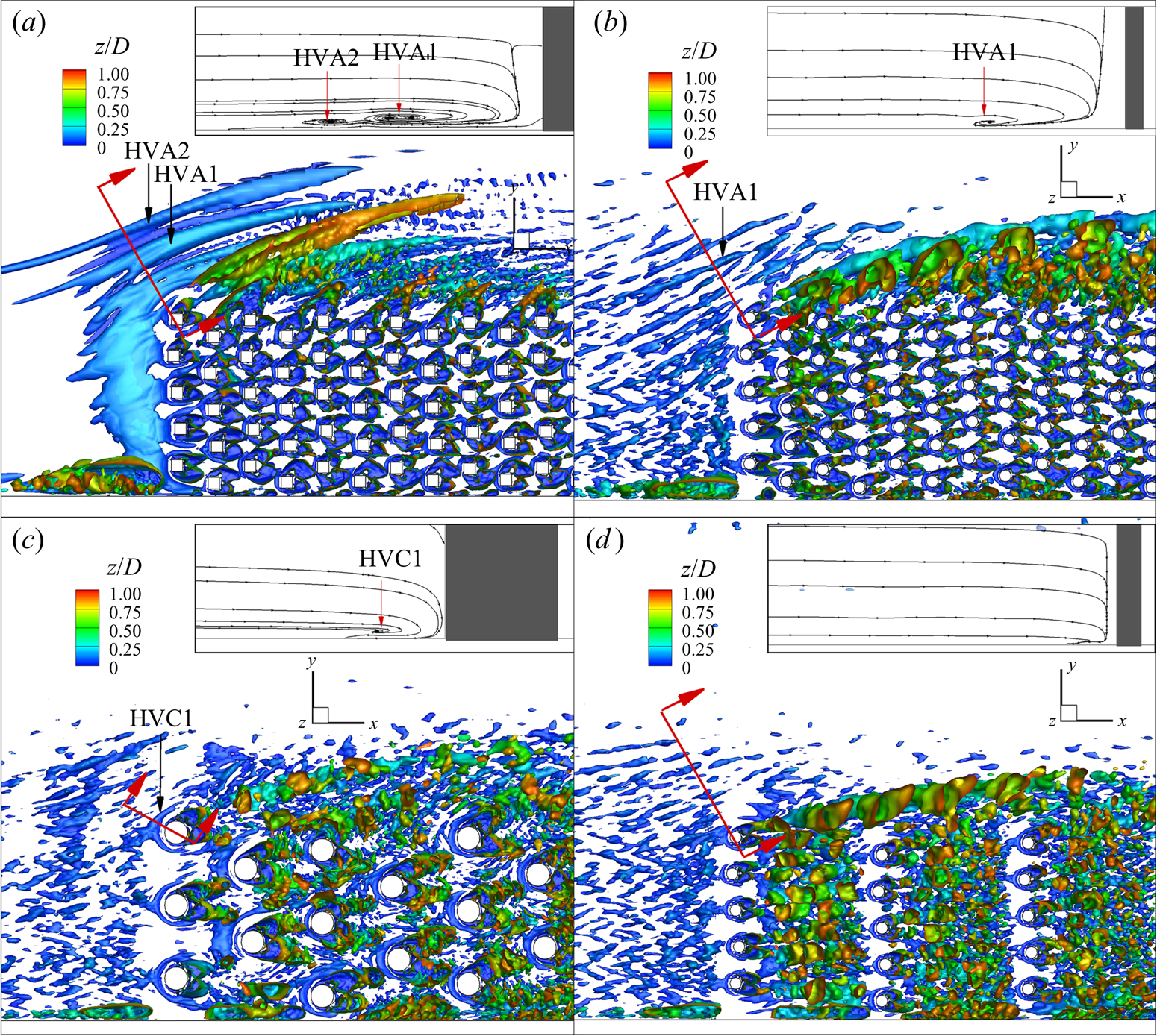
No horseshoe vortex system associated with the array forms in the simulations with circular cylinders if aW < 1 (figure 14c,d). However, horseshoe vortices form around the base of some of the exposed cylinders at the front face of the array if aW < 1 (e.g. HVC1 in figure 14c is a horseshoe vortex associated with the cylinder positioned at the corner of the array). In the case of a loose bed, the individual scour holes forming around the upstream cylinders can grow and start merging with neighbouring ones. This can lead to the formation of a horseshoe vortex around the upstream face of the array during the later stages of the scour process even though no such vortex is present during the initial stages.

6.2. Bed friction velocity and effect of large-scale coherent motions

As the mesh spacing in the vertical direction is small enough for the first point off the wall to be situated inside the viscous sublayer, the magnitude of the local bed friction velocity in the instantaneous flow is calculated as

(6.1)\begin{equation}{u_\tau }/U = {\left( {\frac{1}{{R{e_D}}}\frac{{\frac{{{u_m}}}{U}}}{{\frac{{{n_1}}}{D}}}} \right)^{1/2}},\end{equation}

where u_m is the velocity magnitude in a plane parallel to the bed situated at a normal distance n ₁ from the bed.

As discussed in § 4.1, the passage of the shear layer vortices triggers the formation of regions of high and low streamwise velocity above the channel bed. These regions penetrate until the bed. It is not the cores of the shear layer vortices, but rather the successive regions of high and low, near-bed streamwise velocity that are responsible for the generation of the spanwise-oriented patches of high and low ${u_\tau }$ inside and outside the array (e.g. see u_τ distributions in figure 15 for x/D > 20). The patches of high ${u_\tau }$ start at the sidewall containing the array and end on the free-stream side, outside of the shear layer. For the circular cylinder cases with d/D = 0.1, as aW and ϕ increase, so does ${u_\tau }$ inside these patches. This is especially the case on the free-stream side, where most of the sediment will be entrained in the case of a loose bed. Moreover, the patches of high ${u_\tau }$ are not destroyed at the end of the array but continue to propagate downstream and can induce lots of sediment entrainment on the side of the channel opposite the array.

Figure 15.

Instantaneous flow bed friction velocity magnitude, u_τ/U. (a) ϕ = 0.08, aW = 1.63, d/D = 0.1; (b) ϕ = 0.02, aW = 0.408, d/D = 0.1.

The other regions containing high ${u_\tau }$ values in figure 15 correspond to the flow acceleration region forming on the outer side of the shear layer starting at the upstream corner of the array and to the upstream part of the array. The amplification of ${u_\tau }$ inside the upstream part of the array is due to the increase in the streamwise velocity as the flow accelerates in between neighbouring cylinders and to the wake vortices shed in the wake of the cylinders for which the flow conditions allow the cylinders to shed strongly coherent vortices. As aW increases, more of the incoming flow is deflected around the upstream corner of the array and lower velocity fluid enters the array (figure 6). This has an opposite effect on the length of the two regions of high ${u_\tau }$ and values of ${u_\tau }$ inside them (figure 15).

The sediment entrainment capacity of the flow is not only a function of the mean bed friction velocity, ${\bar{u}_\tau }$, but also of the root-mean-square of the bed friction velocity, $u_\tau ^{SD}$ which accounts in an approximate way for the effects of large-scale unsteadiness on the bed shear stress (Cheng, Koken & Constantinescu Reference Cheng, Koken and Constantinescu2018). Figure 16 allows understanding the effects of varying aW, ϕ, d/D and the cross-sectional shape of the cylinders on these two variables. The formula used to estimate ${\bar{u}_\tau }$ and $u_\tau ^{SD}$ is the same as that used for ${u_\tau }$ but with u_m being redefined as the mean velocity magnitude and the square root of the TKE, respectively.

Figure 16.

Mean-flow bed friction velocity magnitude, ${\bar{u}_\tau }/U$, and root-mean-square of the bed friction velocity fluctuations $u_\tau ^{SD}/U$. (a) ϕ = 0.1, aW = 1.6, d/D = 0.1 SC; (b) ϕ = 0.08, aW = 1.63, d/D = 0.1; (c) ϕ = 0.08, aW = 0.814, d/D = 0.2; (d) ϕ = 0.02, aW = 0.408, d/D = 0.1.

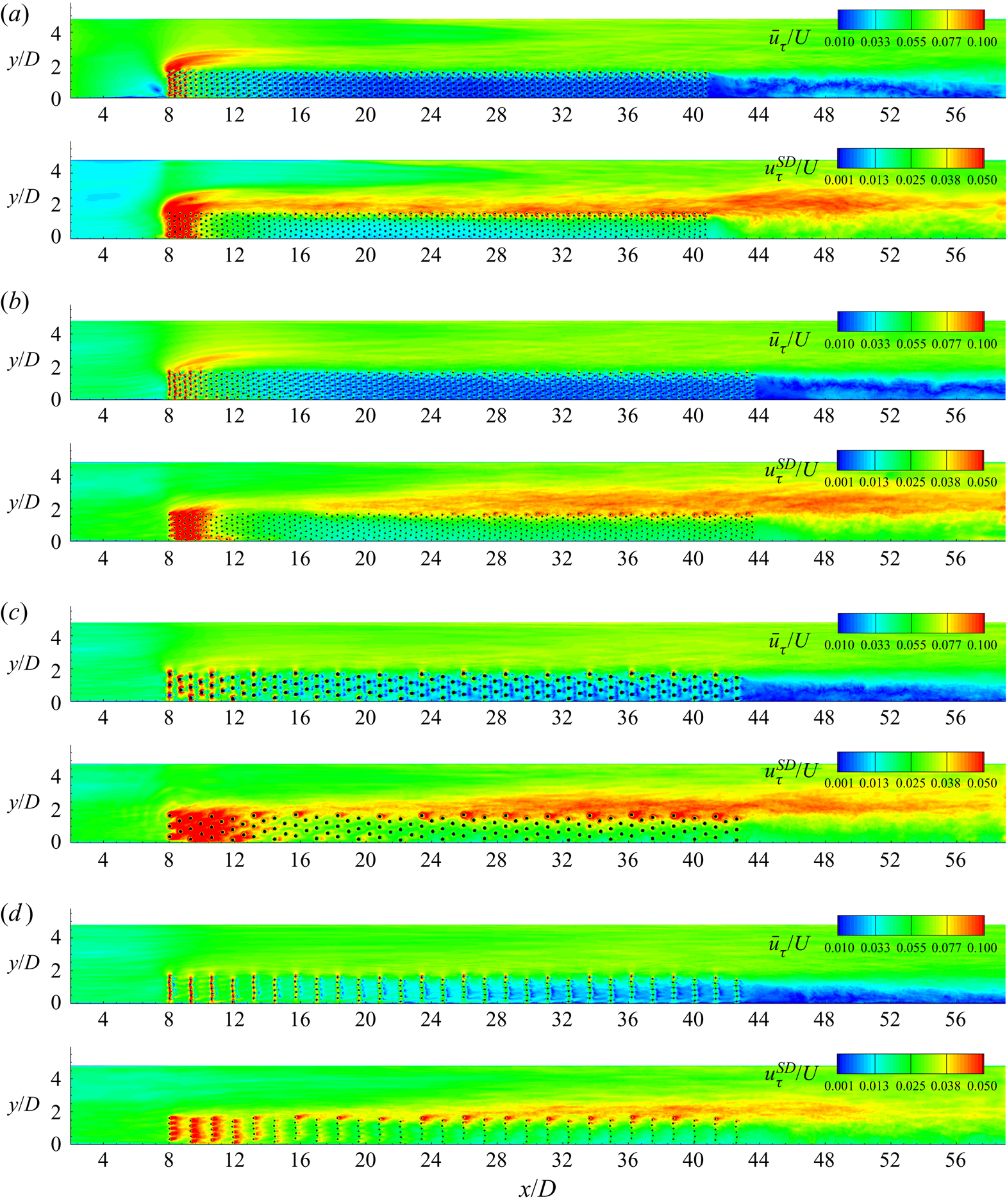
It is only for cases with aW > 1 that a distinct region of high ${\bar{u}_\tau }$ forms on the free-flow side, close to the upstream edge of the array (figure 16a,b). In the two simulations with aW ≈ 1.6, the increase of ${\bar{u}_\tau }$ in this region is by more than 50 % higher in the simulation with square cylinders compared to the one with circular cylinders because the higher bluntness of the cylinders at the front of the patch increase the fraction of the flow approaching the array that is deflected laterally rather than entering the array. The formation of horseshoe vortices (figure 14a) also contributes to the increase of ${\bar{u}_\tau }$ in the same region. As the position and coherence of these vortices change with time, large values of $u_\tau ^{SD}$ are induced inside this region in the aW = 1.6 simulation with square cylinders (figure 16a). The values of $u_\tau ^{SD}$ around the corner of the array remain low in all other simulations which confirms that the amplification of $u_\tau ^{SD}$ in this region is mainly controlled by the horseshoe vortices.

As the velocity inside the horizontal shear layer is lower than that in the remaining part of the free-flow region, one would expect lower ${\bar{u}_\tau }$ values beneath the shear layer compared to the close to constant streamwise velocity region situated close to the sidewall. However, for most cases the levels of ${\bar{u}_\tau }$ beneath the free-stream side of the shear layer are by up to 20 % larger compared to those close to the sidewall (figure 16). This is because of the strong downwelling motions inside the upstream part of the shear layer (figure 11) that advect higher streamwise velocity fluid toward the bed. Meanwhile, the passage of the vortices is responsible for the high values of $u_\tau ^{SD}$ observed in all simulations beneath the horizontal shear layer. The average levels of $u_\tau ^{SD}(x/D)$ tend to level off once the shear layer growth stabilizes and remain high well after the end of the array, as the shear layer vortices maintain their coherence at large distances from the back of the array. The absence of recirculation eddies in the wake of the array (figure 16d) results in a sharper decay of $u_\tau ^{SD}$ in the region behind the array where vortices originating in the shear layer are advected. For constant ϕ or aW, an increase in d/D results in an increase of the average levels of $u_\tau ^{SD}$ inside the stabilized part of the shear layer on the free-stream side (e.g. see figure 16b,c).

The other main region of high $u_\tau ^{SD}$ occupies the upstream part of the patch. It basically corresponds to the region occupied by the cylinders that shed vortices in their wake. Its length increases monotonically with increasing aW, at least for constant d/D. Finally, cylinders situated at the lateral face of the array locally amplify $u_\tau ^{SD}$ along the whole length of the array. For aW < 1, the peak values of $u_\tau ^{SD}$ beneath the shear layer region are induced by the eddies shed by the cylinders at the lateral face of the array rather than by the shear layer vortices (figure 16c,d).

Regions of low ${\bar{u}_\tau }$ and $u_\tau ^{SD}$ favour sediment deposition. Such regions are present inside the array and at its back. Consistent with the streamwise decrease of the streamwise velocity and TKE inside of the array (figures 6 and 10), the length of the region inside the array characterized by a small sediment entrainment capacity increases monotonically with increasing aW. For example, in the simulations with circular cylinders the length of the region with ${\bar{u}_\tau }/U \lt 0.035$ decreases from 25D for aW = 1.63 (figure 16b) to approximately 10D for aW = 0.408 (figure 16d). For same aW, the length of the region of low ${\bar{u}_\tau }$ increases with the increase in the degree of bluntness of the cylinders’ shape (figure 16a,b).

For the range of aW values considered in this study, the wake of the array is a region of low ${\bar{u}_\tau }$ regardless of whether or not recirculation eddies attached to the sidewall form in the wake. In the cases with aW < 1, the region containing the lowest ${\bar{u}_\tau }$ values in the wake of the array remains in the immediate vicinity of the sidewall even when no recirculation eddies are present (figure 16d). A sediment deposition bar is expected to form at the channel bank containing the array and patches of vegetation are expected to grow primarily at their back side because of the supply of nutrients and the low flow velocities in this region.

The maximum values of $u_\tau ^{SD}$ in some large regions inside and around the array (e.g. horizontal shear layer) are close to 50 % of the peak values of ${\bar{u}_\tau }$ (figure 16). This suggests that the sediment entrainment capacity of the flow is significantly affected by the large-scale unsteadiness driven by the coherent structures generated or advected near the bed. Several authors proposed using an augmented bed friction velocity ${\bar{u}_\tau } + Cu_\tau ^{SD}$ in standard sediment entrainment formulas to account for the effect of large-scale unsteadiness, where the empirical coefficient C is close to 1 (Sumer et al. Reference Sumer, Chua, Cheng and Fredsøe2003; Kraft, Wang & Oberlack Reference Kraft, Wang and Oberlack2011; Cheng et al. Reference Cheng, Koken and Constantinescu2018). For example, assuming U = 0.18 m s⁻¹, D = 0.07 m and C = 1, sediment with a mean diameter d ₅₀ = 100 μm is entrained from the bed if $({\bar{u}_\tau } + u_\tau ^{SD})/U \gt 0.067$ using a Shields diagram (Miller, McCave & Komar Reference Miller, McCave and Komar1977).

Two regions of particular interest are the interior of the array and the free-stream region in which the horizontal shear layer vortices are advected. Analysis of the distributions of ${\bar{u}_\tau }/U$ and $u_\tau ^{SD}/U$ inside the array shows that the size of the region defined by $({\bar{u}_\tau } + u_\tau ^{SD})/U \gt 0.067$ is clearly larger in the ϕ = 0.04 and ϕ = 0.08 simulations compared to the other simulations. For the free-stream region around the array, the size of the region defined by $({\bar{u}_\tau } + u_\tau ^{SD})/U \gt 0.067$ peaks for the ϕ = 0.08 simulations. These results suggest that scour around and inside the rectangular array will develop the fastest for arrays with ϕ ≈ 0.08, at least during the initial stages of the scour process, assuming an initial flat-bed surface.

7. Drag forces

The time-averaged, non-dimensional force vector acting on the solid cylinders situated close to the front face of the array,

(7.1)\begin{equation}\frac{{{{\bar{\boldsymbol{F}}}^{\boldsymbol{n}}}}}{{0.5\rho {U^2}dD}} = \frac{{\bar{F}_{DS}^n}}{{0.5\rho {U^2}dD}}\boldsymbol{i} + \frac{{\bar{F}_{DL}^n}}{{0.5\rho {U^2}dD}}\boldsymbol{j} = \bar{F}^{\prime n}_{DS}\boldsymbol{i} + \bar{F}^{\prime n}_{DL}\,\boldsymbol{j}\end{equation}

(n = 1, N, DS and DL denote the streamwise and lateral drag force components, respectively, the bar denotes a time-averaged quantity and the prime denotes a non-dimensional quantity), is shown in figure 17 for the aW = 1.63 and aW = 0.408 cases with d/D = 0.1 and circular cylinders. The mean force acting on each cylinder is obtained by integrating the pressure and shear stresses over the cylinder's height. In both cases, the largest drag forces are induced on the cylinders situated close to the front face of the array. Closer to the back face of the array, the cylinders situated near the lateral face of the array are subject to the largest drag forces because of the higher flow velocities inside the shear layer. So, even for very long arrays with large aW or ϕ where $\bar{\bar{u}}$ is very small at large x/D, the total streamwise drag force is expected to mildly increase with the increase in the length of the array. Results in figure 17 suggest that the cylinders situated inside the upstream part of the array contribute the most to the total drag force and the length of the region characterized by relatively large (streamwise) drag forces increases with decreasing ϕ and aW. Except for the cylinders situated close to the front and lateral faces of the array, the lateral force component is less than 10 % of the streamwise component for most of the remaining cylinders in the array.

Figure 17.

Mean non-dimensional drag force ${\bar{\boldsymbol{F}}^{\boldsymbol{n}}}/0.5\rho {U^2}dD$ acting on the solid cylinders situated close to the front face of the array (8 < y/D < 19). (a) ϕ = 0.08, aW = 1.63, d/D = 0.1; (b) ϕ = 0.02, aW = 0.408, d/D = 0.1. The black vector at the top right corner corresponds to the mean (streamwise) non-dimensional drag force predicted on an isolated solid cylinder of same diameter and for same Re_d.

Some of the aforementioned trends are illustrated in a more quantitative way in figure 18(a) that shows the streamwise decay of the spanwise-averaged, non-dimensional, mean streamwise drag force acting on the cylinders, $\overline {\overline {{{F^{\prime}}_{DS}}} } (x/D)$. For each spanwise row of cylinders, the average streamwise location of the cylinders is calculated and then the average streamwise force is estimated based on the streamwise drag force acting on each of the cylinders forming that row. The close to monotonic decay toward a constant streamwise drag force regime is mainly a function of aW. Cases with similar aW values but with different shape of the cylinders or with different d/D are characterized by a close to identical decay of $\overline {\overline {{{F^{\prime}}_{DS}}} } $ with x/D starting a short distance from the front face. As expected, the mean streamwise drag force acting on the first transverse row of cylinders directly exposed to the flow is larger in the aW = 1.6 simulation with square cylinders $(\overline {\overline {{{F^{\prime}}_{DS}}} } (8) \approx 1.5)$ compared to the aW = 1.63 simulation with circular cylinders $(\overline {\overline {{{F^{\prime}}_{DS}}} } (8) \approx 1)$. However, the values of $\overline {\overline {{{F^{\prime}}_{DS}}} } (x/D)$ in the two simulations are very close starting with the second row of cylinders. The average non-dimensional streamwise drag force for the first row of cylinders, that are directly exposed to the incoming flow, is close to 1 for all simulations conducted with circular cylinders, which is approximately 15 % lower than the value expected for an isolated cylinder of same shape at the same Re_d. This happens because the deceleration of the flow in front of the array is stronger than that observed around an isolated cylinder, as most of the cylinders situated close to the front face of the array contribute to the adverse pressure gradients that deflect the incoming flow moving toward the array. Figure 18(a) also allows estimating the streamwise distance from the front of the array needed for $\overline {\overline {{{F^{\prime}}_{DS}}} } $ to reach a close to constant regime. This distance increases from approximately 12D (7.5W) for aW ≈ 1.6 to approximately 26D (16.5W) for aW ≈ 0.814. Such a regime is not reached by the end of the array in the simulation with aW = 0.408, though extrapolation of simulation results suggests a value close to 40D–50D.

Figure 18.

Streamwise drag forces acting on the cylinders forming the rectangular array. (a) Streamwise variation of the mean (spanwise-averaged) non-dimensional streamwise drag force acting on the solid cylinders, $\overline {\overline {{{F^{\prime}}_{DS}}} } $; (b) streamwise drag coefficient for the circular cylinders forming the array, ${C^{\prime}_d}$ vs. cylinder Reynolds number, Re_c, in log-log scale. Both ${C^{\prime}_d}$ and Re_c are defined with $\bar{\bar{u}}$ as the local velocity scale inside the array. Also included in (b) are curves for fully vegetated channels based on the experiments of Tanino & Nepf (Reference Tanino and Nepf2008) and the drag coefficient curve for a smooth, isolated, circular cylinder.

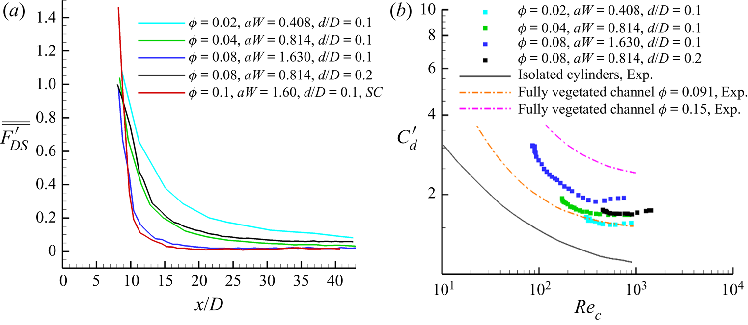
Information on the drag coefficients for the cylinders is important for theoretical models and numerical simulations that do not resolve the flow around the plant stems/cylinders forming the canopy/array. Tanino & Nepf (Reference Tanino and Nepf2008) have shown that for a fully vegetated channel containing rigid emerged cylinders, the cylinder streamwise drag coefficient defined with the mean streamwise velocity inside the array, ${C^{\prime}_d}$, is a function of the cylinder Reynolds number, Re_c, and ϕ for the array. For constant ϕ, the decay of ${C^{\prime}_d}$, with increasing Re_c was qualitatively similar to that observed for isolated cylinders but the drag coefficients were higher (see results for fully vegetated channels and isolated cylinders in figure 18b). A monotonic increase of ${C^{\prime}_d}$, with increasing ϕ was observed for constant Re_c. The present data for rectangular emerged arrays of finite size show that a similar relationship can be established between ${C^{\prime}_d}$, defined with $\bar{\bar{u}}$ as the local velocity scale inside the array, and $R{e_c} = \bar{\bar{u}}d/\nu $ (see figure 18b). Away from the front (high Re_c values) and the back (low Re_c values) of the array, the rate of decrease of ${C^{\prime}_d}$ with Re_c in the simulations conducted with circular cylinders is fairly close to the one determined experimentally by Tanino & Nepf (Reference Tanino and Nepf2008) for fully vegetated channels. Similar to the results of Tanino & Nepf (Reference Tanino and Nepf2008), ${C^{\prime}_d}$ increases with ϕ for constant d and Re_c. The numerical data suggest a monotonic increase of ${C^{\prime}_d}$ with aW for constant Re_c away from the front and back faces of the array.

The finite size of the array induces regions where the flow patterns around the cylinders and the pressure distributions on their surface are very different from those observed in an array occupying the whole channel. For many cylinders that are part of a finite-size emerged array, the mean drag force is not oriented along the streamwise axis of the channel. Moreover, for cylinders situated at about the same streamwise location, the mean streamwise drag force varies significantly across the span of the array. These effects scale mainly with the non-dimensional frontal area per unit volume of the array. For finite-size arrays, the local mean velocity inside the array is different for the cylinders forming the array. In fact, a physically correct and easy to use definition of this variable is impossible to propose for the cylinders situated near the lateral face of the array. For the front face cylinders, the drag coefficient defined with the approaching flow velocity upstream of the array is close to the value expected for isolated cylinders (e.g. close to 1 for the simulations conducted with circular cylinders). However, due to the sharp decay of $\bar{\bar{u}}$ with x/D starting at the front face of the array (figure 6), the values of ${C^{\prime}_d}$ are 50%–100 % larger for the cylinders situated close to the front face compared to the value expected for isolated cylinders. Moreover, these values are up to 15 % higher than the ones one would expect based on extrapolating the ${C^{\prime}_d}$ vs. Re_c variation predicted for the cylinders situated away from the front and back faces of the constant ϕ array (figure 18b). Additionally, an increase of ${C^{\prime}_d}$ is observed for the cylinders with the lowest Re_c values in each simulation compared to the drag coefficients expected based on extrapolating the ${C^{\prime}_d}$ vs. Re_c variation predicted for the cylinders situated away from the front and back faces of the array. This effect is explained by the fact that in a finite-size array the streamwise drag force is not the same for all the cylinders situated in the downstream part of the array where $\bar{\bar{u}}$ and Re_c reach their lowest values and are close to constant. Figure 18b can be used to approximatively estimate drag coefficients for rectangular arrays of different length and width and for different mean channel velocities.

8. Summary and conclusions

The presence of a high length-to-width aspect ratio rectangular array of emerged cylinders at one of the sidewalls of an open channel increases flow three-dimensionality and generates large-scale coherent structures. Most of the relevant flow variables describing flow and turbulence inside the array and the horizontal shear layer and the drag forces acting on the cylinders were found to be mainly a function of the non-dimensional frontal area per unit volume of the array. However, in some cases, marked differences in the streamwise variation of some of the global variables describing flow and turbulence structure inside the array and the horizontal shear layer were observed for arrays with similar aW values but with different diameters of the solid cylinders or for arrays with similar aW values containing solid cylinders of a different shape (e.g. circular vs. square cross-section).

Even if the array contained emerged cylinders, the vertical confinement of the flow in between the bed and the free surface generated strong mean-flow vertical motions especially close to the front face of the array where a downflow forms. As the front face of the array is permeable, the downflow penetrating inside the array induces downwelling inside the corridors of higher velocity magnitude formed in between the cylinders, especially in the region of strong flow divergence situated near the front face of the array. The lateral diversion of part of the incoming flow approaching the array generates downwelling inside the region of high flow acceleration bordering the upstream part of the horizontal shear layer. Meanwhile, strong upwelling is generated in the wakes of the cylinders situated close to the front face of the array and around those situated at its lateral face. For sufficiently high values of aW, a turbulent horseshoe vortex system forms around the upstream base of the array. Together with the vertical velocity fluctuations generated by the large-scale vortical eddies, these 3-D motions affect the availability of nutrients and position of regions where sediment is likely to deposit in the case of a patch of vegetation placed in a loose-bed channel.

Though the lateral face of the array is parallel to the streamwise direction, fluid leaves the array through this boundary over most of its length. The region where the mean transverse velocity component at the lateral interface is oriented toward the free-stream region is not limited to the strongly diverging flow region near the upstream corner of the array. For example, in the aW = 1.6 simulations approximately 50 % of the flow entering the upstream face of the array leaves it through the diverging flow region, but an additional 30 % leaves the array over the part of the lateral boundary where the mean (width- and depth-averaged) streamwise velocity inside the array continues to decay before reaching a constant regime. As aW decreases, the diverging flow region shrinks but the streamwise distance needed for the constant mean streamwise velocity regime to be reached inside the array increases, which means that the finite-length array loses fluid through a larger part of its lateral boundary. The streamwise variations of the streamwise velocity inside the array and of the width-averaged streamwise drag force acting on the cylinders forming the array were found to be mainly a function of aW. Similar to the case of fully vegetated channels, the drag coefficients for the cylinders forming the array were found to be a function of the local cylinder Reynolds number and the array density.

Similar to arrays of emerged circular cylinders placed away from the channel sidewalls, a wake region forms behind the array, the distance between the separated flow region and the back face of the array increases with decreasing aW and the wake flow does not contain recirculation eddies for a sufficiently low aW. For constant aW, the increase in the diameter of the cylinders decreases the size of the separated flow region. The presence of the channel sidewall and the fact that only one shear layer forms if the array is placed adjacent to one of the sidewalls impede the formation and shedding of wake billows. Meanwhile, the shear layer vortices increase their size as they are advected past the end of the array and the distribution of the TKE inside the horizontal shear layer becomes more symmetrical with respect to its centreline defined as the position of the peak TKE.

A main finding of the present study is that the advection of vortices inside the shear layer triggers large-scale wave-like oscillatory motions inside the array. Regions of high and low streamwise velocity form some distance from the front face of the array even before the shear layer width becomes stabilized. Their frequency is approximately half that associated with the advection of the horizontal shear layer vortices. The streamwise velocity wave-like oscillations inside the array trigger the formation of patches of high and low bed friction velocity. In the lateral direction, these patches extend over the regions occupied by the array and the horizontal shear layer. Away from the front face of the array, the regions of highest instantaneous bed friction velocities correspond to the regions of higher streamwise velocities associated with the oscillatory motions. This finding has obvious consequences for sediment entrainment. Our analysis suggests that the formation of large-scale oscillatory motions and the associated effects on the bed shear stress distributions are a general characteristic of shear layers forming at the interface between a porous region and a free-stream region if the interface is fairly aligned with the mean-flow direction in the channel and the width of the porous region is much larger than the penetration width of the shear layer vortices inside the porous region.

The formation of strong upwelling regions at the back of the cylinders for which the local mean streamwise velocity around them is more than 30 % of the mean approaching channel flow velocity upstream of the array and of downwelling motions inside the upstream part of the shear layer(s) on the side(s) of the array appear to be a general characteristic of flow past an emerged array of cylinders, as similar 3-D effects were also observed for circular arrays (Chang et al. Reference Chang, Constantinescu and Tsai2017). Moreover, upwelling and downwelling motions are not restricted to the region situated close to the front face of the array where the downflow forms. Present results for rectangular arrays with a large length-to-width ratio show that the magnitude of the dispersive momentum flux is significant with respect to that of the turbulent flux even away from the front face of the array. So, the momentum transfer within part of the array and near the interface with the free-flow region is affected by 3-D effects (e.g. upwelling and downwelling motions and the associated secondary flow) despite the fact that the geometrical layout would suggest a quasi-2-D flow. This is expected to also be the case for emerged patches of vegetation with a high length-to-width ratio present near one of the channel's banks even if the shape of the patch is not necessarily rectangular or very regular. For such cases, simplified (e.g. depth-averaged) approaches to numerically or theoretically model these flows and data analysis based on field measurements should account for the contribution of the dispersion flux terms to the streamwise (depth-averaged) momentum balance.