


1. Introduction
Waves on the surface of water are a continuing source of fascination, as well as posing an important scientific and engineering challenge, with impacts on such diverse areas as offshore renewables and marine ecology. While we can observe the myriad forms of waves on the water surface, these shapes are only manifestations of what is going on below the surface: a transport of energy and, to a lesser extent, the movement of water particles themselves. Leonardo da Vinci already observed that the wave outruns the water, and early mathematical analyses of wave kinematics seemed to confirm this idea. Work in the early 19th century by Green showed that particle paths in linear deep water waves are approximately circular – in seeming agreement with the exact, deep-water solution derived by Gerstner – and the corresponding finite depth particle paths were shown to be approximately elliptical by Airy (Craik Reference Craik2004).
Nonlinear wave theories began to be explored by Russell, Kelland and, most prominently, Stokes, starting in earnest in the 1840s. It was the work of Stokes that first suggested that particle trajectories in periodic waves in deep water might not be closed and gave rise to the idea of wave-induced motion now known as Stokes drift. In the intervening years, the kinematics of nonlinear waves has received significant attention and the concept of wave-induced drift has taken a prominent role in our understanding of transport in the ocean. Its consequences are still being explored in the movement of floating microplastics (van Sebille et al. Reference van Sebille2020) and water-borne bacteria (Ge et al. Reference Ge, Whitman, Nevers and Phanikumar2012), and we are coming to develop a fuller picture of particle trajectories in nonlinear wave equations (Curtis, Carter & Kalisch Reference Curtis, Carter and Kalisch2018; Carter, Curtis & Kalisch Reference Carter, Curtis and Kalisch2020; Ige & Kalisch Reference Ige and Kalisch2024).
Nevertheless, much remains unknown from both an experimental and theoretical perspective. Experiments are notoriously difficult, owing to the challenge of comparing a closed flume (with no net mass transport and with the additional complication of a mechanical wavemaker) with the situation in the (open) ocean. Recent years have seen significant progress, from flume experiments on monochromatic wave trains (Umeyama Reference Umeyama2012; Paprota & Sulisz Reference Paprota and Sulisz2018), which have been taken to higher and higher steepness (Grue & Kolaas Reference Grue and Kolaas2017), to several recent investigations of particle kinematics for wave groups and complex flows (van den Bremer et al. Reference van den Bremer, Whittaker, Calvert, Raby and Taylor2019; Bjørnestad et al. Reference Bjørnestad, Buckley, Kalisch, Streßer, Horstmann, Frøysa, Ige, Cysewski and Carrasco-Alvarez2021).
Meanwhile, theoretical investigations must contend with the fact that the ubiquitous, Eulerian description of fluid motion – dispensing with particle identity in favour of a simpler treatment of velocity fields – necessarily obscures certain aspects of kinematics. While these difficulties can be circumvented for steady flows by the use of alternative formulations, including employing stream function and velocity potential as independent variables as originally suggested by Stokes, there is no easy fix for non-steady, irregular wave fields. While the pre-eminence of Eulerian theory is being challenged by a resurgence of interest in Lagrangian wave mechanics, including higher-order approximate formulations for steady periodic waves (Clamond Reference Clamond2007), standing waves (Chen & Hsu Reference Chen and Hsu2009) and, recently, wave packets (Abrashkin & Pelinovsky Reference Abrashkin and Pelinovsky2018; Pizzo et al. Reference Pizzo, Lenain, Rømcke, Ellingsen and Smeltzer2023), the vast majority of studies continue to employ the Eulerian perspective. The non-trivial task of comparing the two approaches (Fouques & Stansberg Reference Fouques and Stansberg2008) should not be underestimated.
The aim of this work is to explore the theoretical particle trajectories – and drift – associated with nonlinear potential flow theories in infinite water depth. While there are recent mathematical results for the full, nonlinear problem showing that no closed particle paths exist in steady, periodic wave trains (Constantin Reference Constantin2006; Henry Reference Henry2006; Okamoto & Shoji Reference Okamoto and Shoji2012), these results are not quantitative and are difficult to generalise to non-steady problems. We will take a ‘weakly nonlinear’ approach and our starting point will be the Stokes drift formulation which arises in linear (1st order) water wave theory. While a rigorous proof that linear, steady, periodic water waves exhibit a forward drift in the direction of wave propagation was recently found (Constantin, Ehrnström & Villari Reference Constantin, Ehrnström and Villari2008; Constantin & Villari Reference Constantin and Villari2008), the approximate results due to Stokes are still used in most applications. These were generalised to a spectrum of waves by Kenyon (Reference Kenyon1969) and the resulting formulation has been extensively explored for different spectral shapes (Webb & Fox-Kemper Reference Webb and Fox-Kemper2011), for its sensitivity to the high-frequency spectral tail (Lenain & Pizzo Reference Lenain and Pizzo2020), and new profiles have been developed for practical implementation (Breivik, Bidlot & Janssen Reference Breivik, Bidlot and Janssen2016). Many more references can be found in the recent review by van den Bremer & Breivik (Reference van den Bremer and Breivik2018).
As the Stokes drift formulation comes about through a simplification of the linear water-wave theory, the differences between it and the linear theory are of interest. This also raises a natural question: what if we progress from linear theory to a second- or third-order theory? We expect the higher-order theories to be more accurate and to include important effects for steeper waves – such as the appearance of additional harmonics – which may have a bearing on comparisons with the Stokes drift. Indeed, these theories may suggest improvements to the Stokes drift derived from linear theory. However, with the exception of recent work focusing on wave groups initiated by van den Bremer & Taylor (Reference van den Bremer and Taylor2016), it is difficult to find such comparisons in the literature.
For a successful comparison, we need some way to compute the fluid velocity field $\boldsymbol{u}$
, which drives the particle kinematics through the particle trajectory mapping
$\boldsymbol{u}$
, which drives the particle kinematics through the particle trajectory mapping $\boldsymbol{x}'(t) = \boldsymbol{u}.$
We need a methodology that can deal with several Fourier modes, to simulate irregular seas, and which is accurate to a desired order of nonlinearity. For more than two Fourier modes, the Lagrangian theory is currently limited to second order (Pierson Reference Pierson1961), while important resonant effects in deep water occur only at third order. Consequently, and to increase the accessibility of the results, it seems expedient to work in Eulerian coordinates. Even here, several options exist, including the use of traditional perturbation theory to obtain a solution to the water wave problem, which has been extended to third-order by Madsen & Fuhrman (Reference Madsen and Fuhrman2012). An alternative – which we employ – is to use the equivalent Hamiltonian expansion, which is due to Zakharov (Reference Zakharov1968) and for which the third-order solution has been explored by Zhang & Chen (Reference Zhang and Chen1999) and Gao, Sun & Liang (Reference Gao, Sun and Liang2021). The Hamiltonian expansion furnishes our velocity field and free surface, and these are the tools we use to examine the particle motions.
$\boldsymbol{x}'(t) = \boldsymbol{u}.$
We need a methodology that can deal with several Fourier modes, to simulate irregular seas, and which is accurate to a desired order of nonlinearity. For more than two Fourier modes, the Lagrangian theory is currently limited to second order (Pierson Reference Pierson1961), while important resonant effects in deep water occur only at third order. Consequently, and to increase the accessibility of the results, it seems expedient to work in Eulerian coordinates. Even here, several options exist, including the use of traditional perturbation theory to obtain a solution to the water wave problem, which has been extended to third-order by Madsen & Fuhrman (Reference Madsen and Fuhrman2012). An alternative – which we employ – is to use the equivalent Hamiltonian expansion, which is due to Zakharov (Reference Zakharov1968) and for which the third-order solution has been explored by Zhang & Chen (Reference Zhang and Chen1999) and Gao, Sun & Liang (Reference Gao, Sun and Liang2021). The Hamiltonian expansion furnishes our velocity field and free surface, and these are the tools we use to examine the particle motions.
The remainder of this paper is structured as follows. In § 2, we introduce the water-wave problem and corresponding Hamiltonian. We give more details about the expansion that allows us to extract linear, second- and third-order terms in § 2.1, discuss the neglect of amplitude evolution for our particle kinematics calculations in § 2.2, and finally show how the free surface and potential are obtained to each order in § 2.3. In § 3, we consider monochromatic waves, which is the natural setting to introduce Stokes drift, and look at the consequences of higher-order theories on particle trajectories. Section 4 is devoted to bichromatic waves. These are the simplest type of non-steady wave-field, but because only two harmonics are involved, the linear superposition can be chosen to be periodic. Finally, § 5 considers waves involving multiple lowest-order harmonics. A discussion of the work and some conclusions are presented in § 6. Appendix A adds some comments on the non-uniqueness of the monochromatic Stokes wave solution at third-order, while Appendix B gives expressions for some coefficients appearing in § 2.3. Appendix C explores the effects of slow amplitude evolution on particle paths and Stokes drift.
2. Water-wave problem and Hamiltonian formulation
We begin with the inviscid, irrotational and unidirectional water-wave problem in Eulerian variables. This can be written in terms of a fluid velocity potential $\phi (x,z,t)$
and free surface
$\phi (x,z,t)$
and free surface $\zeta (x,t)$
as
$\zeta (x,t)$
as
 \begin{align} &\Delta \phi = 0\quad \text{ on } -h \lt z \lt \zeta (x,t), \\[-9pt] \nonumber \end{align}
 \begin{align} &\zeta _t + \phi _x \zeta _x = \phi _z \quad\text{ on } z = \zeta (x,t), \\[-9pt] \nonumber \end{align}
 \begin{align} &\phi _t + \frac {1}{2}(\boldsymbol{\nabla }\phi )^2 + g\zeta = 0 \quad\text{ on } z= \zeta (x,t), \\[-12pt] \nonumber \end{align}
 \begin{align} &\phi _z = 0\quad \text{ on } z= -h. \\[9pt] \nonumber \end{align}
The advantage of this formulation is that all nonlinearities have been moved to the boundary conditions, which therefore represent the principal challenge. We also note that, provided the water is deeper than approximately half a typical wavelength, the still-water depth $h$
can be taken to be infinite. (This assumption is innocuous enough if only one wave with fixed length is considered. However, as we shall see later, the interaction of multiple waves in the sea can give rise to long, bound-harmonics, for which the assumption of infinite depth must be critically reassessed.) This procedure, using
$h$
can be taken to be infinite. (This assumption is innocuous enough if only one wave with fixed length is considered. However, as we shall see later, the interaction of multiple waves in the sea can give rise to long, bound-harmonics, for which the assumption of infinite depth must be critically reassessed.) This procedure, using
 \begin{align} \phi _z \rightarrow 0 \quad\text{ as } z \rightarrow \infty \end{align}
in place of (2.1d
) simplifies calculations considerably. Despite the restriction to irrotational flow and the neglect of surface tension, compressibility and viscosity, these equations contain a huge range of interesting physics, including many types of wave phenomena. While the techniques we shall employ can be used without alteration for waves with a transverse ( $y$
) dependence, the additional freedom this engenders means that we defer an exploration of directionally spread waves to future work.
$y$
) dependence, the additional freedom this engenders means that we defer an exploration of directionally spread waves to future work.
During the late 1960s, efforts to find a Hamiltonian formulation of the water wave problem (2.1a )–(2.1d ) came to fruition in work of Zakharov (Reference Zakharov1968) who found the Hamiltonian
 \begin{align} H = \int \int _{-h}^\zeta \frac {1}{2} |\boldsymbol{\nabla }\phi |^2\, {\rm d}z \, {\rm d}x + \int \frac {1}{2}g \zeta ^2 \,{\rm d}x, \end{align}
which represents the total energy of the fluid. The domain of integration in $x$
can, in practice, depend on the specifics of the problem, and the lower boundary of the
$x$
can, in practice, depend on the specifics of the problem, and the lower boundary of the $z$
-integral can be chosen as
$z$
-integral can be chosen as $-\infty$
in place of
$-\infty$
in place of $-h$
if (2.1d′
) is used in place of (2.1d
).
$-h$
if (2.1d′
) is used in place of (2.1d
).
The canonical variables for the Hamiltonian formulation are defined at the free surface. They are $\zeta (x,t)$
and
$\zeta (x,t)$
and ${\phi ^{s}}(x,t)=\phi (x,\zeta (x,t),t),$
and thus the canonical equations are
${\phi ^{s}}(x,t)=\phi (x,\zeta (x,t),t),$
and thus the canonical equations are
 \begin{align} \frac {\partial \zeta }{\partial t} = \frac {\delta H}{\delta {\phi ^{s}}}, \quad \frac {\partial {\phi ^{s}}}{\partial t}=-\frac {\delta H}{\delta \zeta }. \end{align}
These equations are equivalent to the surface boundary conditions (2.1b ), (2.1c ), and details of the calculation can be found in the work of Broer (Reference Broer1974). Additional background can also be found in the recent review by Stuhlmeier (Reference Stuhlmeier and Henry2024).
It is worth noting at the outset that any study of kinematics is necessarily somewhat hampered by the Eulerian variables commonly used in wave research. The Eulerian focus on velocity fields as functions of fixed (laboratory) coordinates obscures the motions of fluid particles, which must be laboriously re-derived. Moreover, as we shall see later, an approximate Eulerian theory divorces the motions of the fluid and the free surface, with consequences for our ability to understand the full kinematics. The alternative choice of Lagrangian variables has many advantages (Pizzo et al. Reference Pizzo, Lenain, Rømcke, Ellingsen and Smeltzer2023; Blaser et al. Reference Blaser, Benamran, Bôas, Lenain and Pizzo2024), but a general Lagrangian theory of nonlinear, irregular waves has yet to be developed, and the connections to the well-established Eulerian theory remain a topic of active exploration.
2.1. Asymptotic analysis and the water-wave problem
The water-wave problem, whether written as a system of partial differential equations and boundary conditions or using the Hamiltonian reformulation, remains mathematically very complex. While the mathematical existence of periodic and solitary wave solutions has been established in ever more general settings (for example, the books by Constantin Reference Constantin2012 or Lannes Reference Lannes2013 offer a relatively recent overview of mathematical progress), much of what is known about qualitative and quantitative properties of ocean waves rests on an analysis of simplified equations.
These simplified equations are usually obtained through so-called asymptotic analysis or perturbation theory – a procedure of non-dimensionalisation and scaling the equations, followed by the identification of small dimensionless parameters, and an asymptotic expansion of the variables in terms of the small parameters selected. In the case of water waves, the most common small parameter is the wave steepness $\epsilon,$
written either as the wave amplitude divided by the wavelength or multiplied by the wavenumber. A very thorough discussion of asymptotic analysis as applied to water waves can be found in the textbook by Johnson (Reference Johnson1997).
$\epsilon,$
written either as the wave amplitude divided by the wavelength or multiplied by the wavenumber. A very thorough discussion of asymptotic analysis as applied to water waves can be found in the textbook by Johnson (Reference Johnson1997).
Instead of expanding the water-wave equations (2.1a )–(2.1d ) in this manner (see Madsen & Fuhrman Reference Madsen and Fuhrman2012 for a detailed, relevant account), it is also possible to expand the Hamiltonian directly. This procedure was carried out by Zakharov (Reference Zakharov1968) and, with more detail, Krasitskii (Reference Krasitskii1994), and it has the advantage of enforcing structure that might otherwise be lost, such as that resulting equations conserve energy.
The first step in this procedure is to write the canonical equations in terms of the Fourier transformed variables $\hat {\zeta }(k)$
and
$\hat {\zeta }(k)$
and $\hat {\phi }(k),$
as
$\hat {\phi }(k),$
as
 \begin{align} \frac {\partial \hat {\zeta }}{\partial t} = \frac {\delta H}{\delta \hat {{\phi ^{s}}}^*}, \quad \frac {\partial \hat {{\phi ^{s}}}}{\partial t} = - \frac {\delta H}{\delta \hat {\zeta }^*}, \end{align}
with $*$
denoting the complex conjugate. Then, one defines a new pair of canonical variables
$*$
denoting the complex conjugate. Then, one defines a new pair of canonical variables $a(k)$
and
$a(k)$
and $ia^*(k)$
related to
$ia^*(k)$
related to $\phi ^{s}$
and
$\phi ^{s}$
and $\zeta$
via Fourier transforms as
$\zeta$
via Fourier transforms as
 \begin{align} \zeta (x) = \frac {1}{2\pi } \int \left ( \frac {q(k)}{2 \omega (k)}\right )^{1/2} \left [ a(k) + a^*(-k)\right ] e^{ikx} \,{\rm d}k, \\[-12pt] \nonumber \end{align}
 \begin{align} {\phi ^{s}}(x) = \frac {-i}{2\pi } \int \left ( \frac {\omega (k)}{2 q(k)}\right )^{1/2} \left [ a(k) - a^*(-k)\right ] e^{ikx} \,{\rm d}k,\\[9pt] \nonumber \end{align}
where
 \begin{align} q(k) = |k| \tanh (|k|h), \end{align} $\omega = \sqrt {gq(k)}$
is the frequency (in rad s−1) and
$\omega = \sqrt {gq(k)}$
is the frequency (in rad s−1) and $g$
is the constant acceleration of gravity (taken to be 9.8 m s−
$g$
is the constant acceleration of gravity (taken to be 9.8 m s− $^2$
in computations). As we will be interested in deep-water waves (
$^2$
in computations). As we will be interested in deep-water waves ( $h\rightarrow \infty )$
, we note that the dispersion relation simplifies to
$h\rightarrow \infty )$
, we note that the dispersion relation simplifies to
 \begin{align} \omega ({k})^2 = g | {k}|. \end{align}
We will use this in all the computations that follow.
The subsequent steps in the expansion are somewhat lengthy and are given by Krasitskii (Reference Krasitskii1994). At this stage, it is important to emphasise only one key point: at lowest order, the problem is linear, so the superposition principle holds. This means that the Fourier amplitudes – which correspond essentially to the magnitudes of the terms $a(k)$
introduced in (2.5)–(2.6) – do not change with time. If gravity is the sole restoring force, the surprising fact is that the Fourier amplitudes do not change with time at the next order either. Only at third-order in nonlinearity, where resonance between quartets of gravity waves becomes possible, do we obtain an evolution equation. This equation gives the slow evolution of the complex amplitude
$a(k)$
introduced in (2.5)–(2.6) – do not change with time. If gravity is the sole restoring force, the surprising fact is that the Fourier amplitudes do not change with time at the next order either. Only at third-order in nonlinearity, where resonance between quartets of gravity waves becomes possible, do we obtain an evolution equation. This equation gives the slow evolution of the complex amplitude $b_0=b(k_0,t),$
 \begin{align} i \frac {\partial b_0}{\partial t} = \omega _0 b_0 + \int \tilde {V}^{(2)}_{0123} b_1^* b_2 b_3 \delta _{0+1-2-3}\, {\rm d}k_{123}, \end{align}
and is known as the Zakharov equation, with a kernel term $\tilde {V}^{(2)}$
given by Krasitskii (Reference Krasitskii1994, (3.5)). We have introduced subscript notation to denote wavenumbers, so that, for example, the delta-function
$\tilde {V}^{(2)}$
given by Krasitskii (Reference Krasitskii1994, (3.5)). We have introduced subscript notation to denote wavenumbers, so that, for example, the delta-function $\delta _{0+1-2-3}$
is a shorthand for
$\delta _{0+1-2-3}$
is a shorthand for $\delta (k_0 + k_1 - k_2 - k_3).$
In principle,
$\delta (k_0 + k_1 - k_2 - k_3).$
In principle, $k_i$
can be either a scalar or a vector wavenumber, although our computations will deal only with the scalar case for simplicity.
$k_i$
can be either a scalar or a vector wavenumber, although our computations will deal only with the scalar case for simplicity.
If $b$
is known, then the canonical variable
$b$
is known, then the canonical variable $a$
can be recovered via
$a$
can be recovered via
 \begin{align} a_0 = b_0 &+ \int A^{(1)}_{012} b_1 b_2 \delta _{0-1-2}\, {\rm d}k_{12} + \int A^{(2)}_{012} b_1^* b_2 \delta _{0+1-2} \,{\rm d}k_{12} + \int A^{(3)}_{012} b_1^* b_2^* \delta _{0+1+2} \,{\rm d}k_{12} \nonumber \\ &+ \int B^{(1)}_{0123} b_1 b_2 b_3 \delta _{0-1-2-3}\, {\rm d}k_{123} + \int B^{(2)}_{0123} b_1^* b_2 b_3 \delta _{0+1-2-3} \,{\rm d}k_{123} \nonumber \\ &+ \int B^{(3)}_{0123} b_1^* b_2^* b_3 \delta _{0+1+2-3}\, {\rm d}k_{123} + \int B^{(4)}_{0123} b_1^* b_2^* b_3^* \delta _{0+1+2+3}\, {\rm d}k_{123} + \cdots, \end{align}
where we have written terms up to third order only. This expression is given by Krasitskii (Reference Krasitskii1994, (2.17)), as are the relevant interaction kernels $A^{(i)}, \, B^{(i)}$
. Finally, once
$A^{(i)}, \, B^{(i)}$
. Finally, once $a$
is known, it is possible to recover
$a$
is known, it is possible to recover $\zeta$
and
$\zeta$
and $\phi ^{s}$
up to the desired order by means of (2.5)–(2.6).
$\phi ^{s}$
up to the desired order by means of (2.5)–(2.6).
2.2. Constant magnitude approximation
The procedure outlined previously would seem to suggest that we first need to solve the complicated integro-differential Zakharov equation (2.9). In fact, for certain situations of interest, we can circumvent this step. The key insight is that the evolution described by the Zakharov equation – being associated with cubic nonlinearities – occurs on the slow time scale $\epsilon ^{-2} T$
, where
$\epsilon ^{-2} T$
, where $\epsilon$
is a typical wave steepness and
$\epsilon$
is a typical wave steepness and $T$
is a typical wave period. For processes taking place on faster time scales, it may be appropriate to consider the complex amplitudes to be constant.
$T$
is a typical wave period. For processes taking place on faster time scales, it may be appropriate to consider the complex amplitudes to be constant.
This is indeed the approach we will adopt. There is, however, one important addition: for certain wavenumber combinations, the Zakharov equation (2.9) can be solved explicitly. In particular, for all symmetric quartets which satisfy $k_0 + k_0 = k_0 + k_0$
or
$k_0 + k_0 = k_0 + k_0$
or $k_0 + k_1 = k_0 + k_1$
, the equation reduces to a system of one or two ordinary differential equations with constant-amplitude solutions, as shown by Mei, Stiassnie & Yue (Reference Mei, Stiassnie and Yue2018, Ch. 14). Such solutions represent nonlinear corrections to the frequency of the waves and were first found by Stokes for a single wave mode. For arbitrarily many modes, or a continuous spectrum, it is possible to write these corrections in a compact form (Stuhlmeier & Stiassnie Reference Stuhlmeier and Stiassnie2019).
$k_0 + k_1 = k_0 + k_1$
, the equation reduces to a system of one or two ordinary differential equations with constant-amplitude solutions, as shown by Mei, Stiassnie & Yue (Reference Mei, Stiassnie and Yue2018, Ch. 14). Such solutions represent nonlinear corrections to the frequency of the waves and were first found by Stokes for a single wave mode. For arbitrarily many modes, or a continuous spectrum, it is possible to write these corrections in a compact form (Stuhlmeier & Stiassnie Reference Stuhlmeier and Stiassnie2019).
Incorporating these corrections means that the complex amplitudes $b_i(t)$
have constant magnitudes but time-dependent phases,
$b_i(t)$
have constant magnitudes but time-dependent phases,
 \begin{align} b_i(t) = |b_i(0)| \exp \bigg ({-}it \bigg [ \tilde {V}^{(2)}_{\textit{iiii}} |b_i(0)|^2 + 2 \sum _{j\neq i} \tilde {V}^{(2)}_{\textit{ijij}} |b_j(0)|^2 \bigg ] \bigg ). \end{align}
The terms in the argument of the exponential reduce to $\omega a^2 k^2/2$
, the well-known Stokes’ correction, when only a single wave-mode is present, or the mutual frequency correction found by Longuet-Higgins & Phillips (Reference Longuet-Higgins and Phillips1962) for two modes. The form (2.11) now contains all the mutual dispersion corrections of the cubically nonlinear water-wave theory. It has been demonstrated that taking these corrections into account allows one to predict the short-time propagation of laboratory waves with high accuracy without the need to solve for the evolution of the slow-time variables (Galvagno, Eeltink & Stuhlmeier Reference Galvagno, Eeltink and Stuhlmeier2021; Stuhlmeier & Stiassnie Reference Stuhlmeier and Stiassnie2021; Meisner et al. Reference Meisner, Galvagno, Andrade, Liberzon and Stuhlmeier2023), showing that the constant magnitude approximation is well justified for such cases. Of course, under specific circumstances – for example, with a sufficiently narrow spectrum or close to modulation instability – we may have significant energy transfer (Andrade & Stuhlmeier Reference Andrade and Stuhlmeier2023). However, given our focus on particle paths (with a characteristic time of the order of one period), the amplitude evolution will be considered to be negligible (see also the discussion by Stuhlmeier & Stiassnie (Reference Stuhlmeier and Stiassnie2019) and Appendix A therein).
$\omega a^2 k^2/2$
, the well-known Stokes’ correction, when only a single wave-mode is present, or the mutual frequency correction found by Longuet-Higgins & Phillips (Reference Longuet-Higgins and Phillips1962) for two modes. The form (2.11) now contains all the mutual dispersion corrections of the cubically nonlinear water-wave theory. It has been demonstrated that taking these corrections into account allows one to predict the short-time propagation of laboratory waves with high accuracy without the need to solve for the evolution of the slow-time variables (Galvagno, Eeltink & Stuhlmeier Reference Galvagno, Eeltink and Stuhlmeier2021; Stuhlmeier & Stiassnie Reference Stuhlmeier and Stiassnie2021; Meisner et al. Reference Meisner, Galvagno, Andrade, Liberzon and Stuhlmeier2023), showing that the constant magnitude approximation is well justified for such cases. Of course, under specific circumstances – for example, with a sufficiently narrow spectrum or close to modulation instability – we may have significant energy transfer (Andrade & Stuhlmeier Reference Andrade and Stuhlmeier2023). However, given our focus on particle paths (with a characteristic time of the order of one period), the amplitude evolution will be considered to be negligible (see also the discussion by Stuhlmeier & Stiassnie (Reference Stuhlmeier and Stiassnie2019) and Appendix A therein).
If we sum up the consequences of weak-nonlinearity in the Fourier description of surface gravity waves in deep water as:
-
(1) dispersion corrections;
-
(2) changes to wave shape (bound harmonics);
-
(3) energy exchange between modes,
we will account for items (1) and (2) while neglecting the slow effects of item (3). Only the amplitude-dependence of the dispersion relation is a general property of nonlinear waves. The other effects arise from the viewpoint of Fourier analysis. Solitary waves, for example, do not have a counterpart in linear theory whose ‘shape’ is modified by the inclusion of higher-order effects. Appendix C provides some further discussion of the neglect of amplitude evolution, along with several examples.
2.3. Recovery of the third-order solution
The Hamiltonian formulation makes clear how the free surface and potential can be recovered from the canonical variables $a(k)$
and
$a(k)$
and $a^*(k)$
up to a given order. In practice, discrete wavenumbers are considered, which means that the integrals in (2.10) can be simplified by the substitution
$a^*(k)$
up to a given order. In practice, discrete wavenumbers are considered, which means that the integrals in (2.10) can be simplified by the substitution
 \begin{align} b(k) = \sum _i B_i \delta (k-k_i). \end{align}
Here $B_i=B(k_i,t)$
is unknown in principle and, in practice, comes from a constant magnitude approximation to (2.9) as discussed in § 2.2.
$B_i=B(k_i,t)$
is unknown in principle and, in practice, comes from a constant magnitude approximation to (2.9) as discussed in § 2.2.
Because the free surface equation (2.5) is recovered directly from substitution of (2.10), it is clear that we can distinguish linear, quadratic and cubic terms in $\zeta$
based on the respective terms in (2.10). The same is not true of
$\zeta$
based on the respective terms in (2.10). The same is not true of $\phi$
, as we shall see later. Taking the inverse Fourier transform yields
$\phi$
, as we shall see later. Taking the inverse Fourier transform yields
 \begin{align} \zeta _1 = \frac {1}{2 \pi } \sum _i \sqrt {\frac {\omega _i}{2g}} A_i \big ( e^{i \xi _i} + e^{-i \xi _i} \big ). \end{align}
Here, we have substituted $B_i = A_i e^{-i\varphi _i(t)}$
with amplitude
$B_i = A_i e^{-i\varphi _i(t)}$
with amplitude $A_i \in \mathbb{R}$
and phase
$A_i \in \mathbb{R}$
and phase $\varphi _i(t),$
and employ the compact notation
$\varphi _i(t),$
and employ the compact notation $\xi _i = k_i x - \varOmega _i t + \theta _i.$
Clearly, this yields the expected sinusoidal free surface elevation upon defining the amplitude
$\xi _i = k_i x - \varOmega _i t + \theta _i.$
Clearly, this yields the expected sinusoidal free surface elevation upon defining the amplitude
 \begin{align} \frac {1}{\pi } \sqrt {\frac {\omega _i}{2g}} A_i = a_i. \end{align}
The nonlinear corrected frequency is given by
 \begin{align} \varOmega _i = \omega _i + \tilde {V}^{(2)}_{\textit{iiii}} |A_i|^2 + 2 \sum _{j\neq i} \tilde {V}^{(2)}_{\textit{ijij}} |A_j|^2, \end{align}
and for unidirectional waves in infinite depth – which will be our focus – we can simplify the kernels to
 \begin{align} \tilde {V}^{(2)}_{\textit{iiii}} = \frac {1}{4 \pi ^2} k_i^3 \text{ and } \tilde {V}^{(2)}_{\textit{ijij}} = \frac {1}{4 \pi ^2} k_i k_j \min (k_i,k_j). \end{align}
The quadratic components of the free surface elevation can be obtained in analogous manner, with slightly more in the way of algebra required to resolve all delta-functions. We find
 \begin{align} \zeta _2(x,t) = & \frac {1}{2\pi } \sum _{i,j} A_i A_j \left \lbrace \sqrt {\frac {\omega _{i+j}}{2g}} \left ( A^{(1)}_{i+j,i,j} + A^{(3)}_{-i-j,i,j} \right ) \big [ e^{i(\xi _i + \xi _j)} + e^{-i(\xi _i + \xi _j)} \big ] \right . \nonumber \\ & \left . + \sqrt {\frac {\omega _{i-j}}{2g}} A^{(2)}_{j-i,i,j} \big [ e^{i(\xi _j-\xi _i)} + e^{i(\xi _i-\xi _j)} \big ] \right \rbrace . \end{align}
The shorthand notation $\omega _{i\pm j}$
is used to denote
$\omega _{i\pm j}$
is used to denote $\omega (k_i \pm k_j) = \sqrt {g |k_i \pm k_j|}.$
We can write the cubic components of the free surface elevation as
 \begin{align} \zeta _3(x,t) = & \frac {1}{2 \pi } \sum _{i,j,k} A_i A_j A_k \left \lbrace \sqrt {\frac {\omega _{i+j+k}}{2g}} \left ( B^{(1)}_{i+j+k,i,j,k} + B^{(4)}_{-i-j-k,i,j,k} \right ) \big [ e^{i(\xi _i + \xi _j + \xi _k)} \big . \right . \nonumber \\& \left. \big . + e^{-i(\xi _i + \xi _j + \xi _k)} \big ] + \sqrt {\frac {\omega _{i-j-k}}{2g}} B^{(2)}_{j+k-i,i,j,k} \big [ e^{i(\xi _j+\xi _k-\xi _i)} + e^{i(\xi _i -\xi _j - \xi _k)} \big ] \right . \nonumber \\& \left . + \sqrt {\frac {\omega _{i+j-k}}{2g}} B^{(3)}_{k-i-j,i,j,k} \big [ e^{i(\xi _k-\xi _i-\xi _j)} + e^{i(\xi _i+\xi _j-\xi _k)} \big ] \right \rbrace . \end{align}
The velocity potential at the free surface, $\phi ^{s}$
, is obtained from (2.6) via an identical procedure.
$\phi ^{s}$
, is obtained from (2.6) via an identical procedure.
The contributions of the second-order and third-order free surface elevation change only the wave shape. The resulting harmonics of the form $\exp (i(\xi _i \pm \xi _j))$
behave as waves with wavenumber
$\exp (i(\xi _i \pm \xi _j))$
behave as waves with wavenumber $k_i \pm k_j$
and frequency
$k_i \pm k_j$
and frequency $\varOmega _i \pm \varOmega _j,$
but because these sums and differences do not satisfy the dispersion relation, they are referred to as ‘bound waves’, in contrast to the free waves of (2.13). The impact of these bound waves on sharpening the crests and flattening the troughs is shown in figure 1 for a bichromatic sea, together with the effect of the third-order frequency correction (2.15) on the wave phases. We also note the important effect of the difference harmonic terms
$\varOmega _i \pm \varOmega _j,$
but because these sums and differences do not satisfy the dispersion relation, they are referred to as ‘bound waves’, in contrast to the free waves of (2.13). The impact of these bound waves on sharpening the crests and flattening the troughs is shown in figure 1 for a bichromatic sea, together with the effect of the third-order frequency correction (2.15) on the wave phases. We also note the important effect of the difference harmonic terms $k_i-k_j$
in creating a ‘set-down’ below the crest, see van den Bremer et al. (Reference van den Bremer, Whittaker, Calvert, Raby and Taylor2019).
$k_i-k_j$
in creating a ‘set-down’ below the crest, see van den Bremer et al. (Reference van den Bremer, Whittaker, Calvert, Raby and Taylor2019).
2.3.1. Recovery of the bulk potential
The reformulation of the problem in surface variables is very convenient from many perspectives, but is something of a disadvantage when we wish to recover information about the bulk fluid below the free surface. To obtain this, we start with the general solution of the Laplace equation which decays for infinite depth
 \begin{align} \phi (x,z) = \frac {1}{2\pi } \int \phi (k) e^{kz} e^{ikx}\, {\rm d}k, \quad \phi (k) = \phi ^*(-k), \end{align}
the exact analogue of Krasitskii (Reference Krasitskii1994, (4.1)).
Free surface of a bichromatic wave train with linear frequencies $\omega _1=1$
rad s−1 and
$\omega _1=1$
rad s−1 and $\omega _2=1.25$
rad s−1, and wave slopes
$\omega _2=1.25$
rad s−1, and wave slopes $\epsilon _1=\epsilon _2=0.15,$
showing first-order (linear), second-order and third-order solutions and their bound wave (B.W.) constituents. Note the phase shift appearing at third order due to the frequency correction (4.4)–(4.5).
$\epsilon _1=\epsilon _2=0.15,$
showing first-order (linear), second-order and third-order solutions and their bound wave (B.W.) constituents. Note the phase shift appearing at third order due to the frequency correction (4.4)–(4.5).

We relate the bulk potential $\phi$
and its surface trace
$\phi$
and its surface trace $\phi ^{s}$
to one another in terms of an expansion. Taking the problem in infinite depth, we need to solve
$\phi ^{s}$
to one another in terms of an expansion. Taking the problem in infinite depth, we need to solve
 \begin{align} &\Delta \phi = 0, \\[-12pt] \nonumber \end{align}
 \begin{align} &\phi = {\phi ^{s}}\quad \text{ on } z = \zeta , \\[-12pt] \nonumber \end{align}
 \begin{align} &\phi _z \rightarrow 0 \quad\text{ as } z \rightarrow -\infty , \\[9pt] \nonumber \end{align}
which we do by assuming the free surface elevation is small ( $\zeta \rightarrow \epsilon \zeta$
) and then inserting this expansion into the boundary condition (2.21), so that
$\zeta \rightarrow \epsilon \zeta$
) and then inserting this expansion into the boundary condition (2.21), so that
 \begin{align} \phi (\zeta ) = \phi (0) + \epsilon \zeta \phi _z(0) + \frac {\epsilon ^2 \zeta ^2}{2} \phi _zz(0) + \cdots . \end{align}
This gives rise to a hierarchy of problems in physical space, whose successive solution yields
 \begin{align} \hat {\phi }(k,z,t) = e^{|k|z} \left [ \hat {\phi }^s - \frac {1}{2 \pi } \int \hat {\zeta }_1 \hat {\phi }^s_2 |k_2| \delta _{0-1-2}\, {\rm d}k_{12} - \int D_{0123} \hat {\phi }^s_1 \hat {\zeta }_2 \hat {\zeta }_3 \delta _{0-1-2-3} \,{\rm d}k_{123} + \cdots \right ], \end{align}
with
 \begin{align} D_{0123} = -\frac {1}{4} |k_1| \left ( 2 |k_1| - |k_1 + k_2| - |k_1 + k_3| - |k_0-k_3| - |k_0-k_2| \right ). \end{align}
With $\hat {{\phi ^{s}}}$
and
$\hat {{\phi ^{s}}}$
and $\hat {\zeta }$
known from the formulation in (2.5)–(2.6), we can now recover the bulk potential at each order desired. This procedure is also detailed by Janssen (Reference Janssen2004, below (4.7)), Krasitskii (Reference Krasitskii1994, p.15) and Zakharov (Reference Zakharov1968, (1.8)), although care should be taken in the symmetrisation of (2.25).
$\hat {\zeta }$
known from the formulation in (2.5)–(2.6), we can now recover the bulk potential at each order desired. This procedure is also detailed by Janssen (Reference Janssen2004, below (4.7)), Krasitskii (Reference Krasitskii1994, p.15) and Zakharov (Reference Zakharov1968, (1.8)), although care should be taken in the symmetrisation of (2.25).
The linear contribution consists simply of the first term in (2.24),
 \begin{align} \phi _1(x,z,t) = \frac {1}{\pi } \sum _i A_i e^{|k_i|z} \sqrt {\frac {g}{2\omega _i}} \sin (\xi _i). \end{align}
The quadratic contribution is
 \begin{align} \phi _2(x,z,t) & = \sum _{i,j} A_i A_j \left [ \mathcal{C}^{(2)}_{i+j} \sin (\xi _i + \xi _j) e^{|k_i+k_j|z} + \mathcal{C}^{(2)}_{i-j} \sin (\xi _i - \xi _j) e^{|k_i-k_j|z} \right ], \end{align}
where we need to employ the linear and quadratic parts of $\hat {\phi }^s$
and
$\hat {\phi }^s$
and $\hat {\zeta }$
(and products thereof) in the formulation. The coefficients
$\hat {\zeta }$
(and products thereof) in the formulation. The coefficients $\mathcal{C}^{(2)}$
are given in Appendix B. Up to second order, for unidirectional waves in deep water, the potential reduces to the simple expression
$\mathcal{C}^{(2)}$
are given in Appendix B. Up to second order, for unidirectional waves in deep water, the potential reduces to the simple expression
 \begin{align} \phi = \sum _j \frac {a_j g}{\omega _j} e^{|k_j|z} \sin ( k_j x - \omega _j t) - \sum _{i\gt j} \omega _{i} a_i a_j \sin (\xi _{i} - \xi _{j} ) e^{|k_i - k_j| z}, \end{align}
which follows also from Dalzell (Reference Dalzell1999).
The cubic contribution to the bulk potential is
 \begin{align} \phi _3(x,z,t) &= \sum _{ijk} A_i A_j A_k \left \lbrace \mathcal{C}^{(3)}_{i+j+k} \sin (\xi _i+\xi _j+\xi _k) e^{|k_i+k_j+k_k|z} \right . \nonumber \\ &+ \mathcal{C}^{(3)}_{i-j-k} \sin (\xi _i-\xi _j-\xi _k) e^{|k_i-k_j-k_k|z} \left . + \mathcal{C}^{(3)}_{i+j-k} \sin (\xi _i + \xi _j - \xi _k) e^{|k_i+k_j-k_k|z} \right . \nonumber \\ &+ \left . \mathcal{C}^{(3)}_{i-j+k} \sin (\xi _i-\xi _j+\xi _k) e^{|k_i-k_j+k_k|z} \right \rbrace . \end{align}
The coefficients $\mathcal{C}^{(3)}$
are given in Appendix B. Unfortunately, efforts to find a compact simplification for the third order have failed except in the case of a single monochromatic wave, where the analytical expression
$\mathcal{C}^{(3)}$
are given in Appendix B. Unfortunately, efforts to find a compact simplification for the third order have failed except in the case of a single monochromatic wave, where the analytical expression
 \begin{align} \phi _3 = -\frac {a^3 \omega k}{4} e^{kz} \sin \xi \end{align}
is recovered (see Gao et al. Reference Gao, Sun and Liang2021 and Appendix A).
It should be emphasised that the bulk potential thus obtained is equivalent (except for the non-uniqueness at a given order mentioned in Appendix A) to the potential found through direct perturbation expansion of the governing equations (2.1a
)–(2.1d′
). In particular, as we shall see later, this means that the fluid domain at each order is the half-space $\{ (x,z) \mid x\in \mathbb{R}, z\leq 0 \},$
owing to the transfer of the boundary conditions.
$\{ (x,z) \mid x\in \mathbb{R}, z\leq 0 \},$
owing to the transfer of the boundary conditions.
3. Monochromatic waves
The mathematically simplest type of wave motion, and the one about which we know the most, is that of steady, periodic waves known as Stokes waves. For such waves, symmetric about a crest and propagating without change of form, it can be proven that no closed particle trajectories exist (Constantin Reference Constantin2006) and explicit calculations of the surface drift have been given by Longuet-Higgins (Reference Longuet-Higgins1987) up to and including the wave of greatest height. This wealth of prior results means that we do not strictly need the Hamiltonian expansion developed in § 2; however, we shall attempt to situate the third-order theory and its predictions among other results for monochromatic waves.
Because the waveform is steady, and the fluid motion is periodic and confined to the $(x,z)$
-plane, a variety of powerful mathematical techniques exist for tackling the problem, including the use of the velocity potential and stream function as independent variables (Stokes Reference Stokes2009). Moreover, the convergence of perturbative solutions for such waves has been established since the work of Levi-Civita (Reference Levi-Civita1925) and, in practice, such solutions have been computed to extremely high order (Schwartz Reference Schwartz1974).
$(x,z)$
-plane, a variety of powerful mathematical techniques exist for tackling the problem, including the use of the velocity potential and stream function as independent variables (Stokes Reference Stokes2009). Moreover, the convergence of perturbative solutions for such waves has been established since the work of Levi-Civita (Reference Levi-Civita1925) and, in practice, such solutions have been computed to extremely high order (Schwartz Reference Schwartz1974).
Thus, if we fix the wave length (or wavenumber) and the wave height $H,$
the successive inclusion of higher-order terms brings us ever closer to the exact solution. This appears to be true also when we employ the equivalent Lagrangian formulation of fluid mechanics (Clamond Reference Clamond2007), albeit without the accompanying analytical theory proving convergence. Some care must be taken in the selection of expansion parameter (in which the ‘order’ is measured), as discussed by Cokelet (Reference Cokelet1977) and Fenton (Reference Fenton1985), about which more will be said in the following.
$H,$
the successive inclusion of higher-order terms brings us ever closer to the exact solution. This appears to be true also when we employ the equivalent Lagrangian formulation of fluid mechanics (Clamond Reference Clamond2007), albeit without the accompanying analytical theory proving convergence. Some care must be taken in the selection of expansion parameter (in which the ‘order’ is measured), as discussed by Cokelet (Reference Cokelet1977) and Fenton (Reference Fenton1985), about which more will be said in the following.
Although these steady, periodic waves are theoretically exceptional and experimentally difficult to realise, the wealth of accumulated understanding makes them an ideal starting point and allows for comparisons that will stand us in good stead for later, unsteady problems. We start by reproducing the textbook monochromatic solution (Dean & Dalrymple Reference Dean and Dalrymple1991) to the linearised governing equations (2.1a )–(2.1d′ ) in the Eulerian description:
 \begin{align} & \zeta _1 = a \cos (\xi ), \quad \phi _1 = \frac {a\omega }{k} e^{kz} \sin (\xi ), \end{align}
where $\xi =kx-\omega t$
and
$\xi =kx-\omega t$
and
 \begin{align} \omega ^2 = g|k| \end{align}
is the linear dispersion relation. Here, $z\leq 0$
and
$z\leq 0$
and $x \in \mathbb{R}.$
If the gradient of
$x \in \mathbb{R}.$
If the gradient of $\phi _1$
from (3.1) is evaluated to yield the velocity field, it is evident that the average over a wave period
$\phi _1$
from (3.1) is evaluated to yield the velocity field, it is evident that the average over a wave period $T$
– called the Eulerian mean velocity and whose horizontal component is denoted by
$T$
– called the Eulerian mean velocity and whose horizontal component is denoted by $u_E$
– vanishes at every depth
$u_E$
– vanishes at every depth $z\leq 0$
.
$z\leq 0$
.
Just because the average velocity measured by a fixed sensor vanishes does not mean that a particle released at the sensor location returns there after one wave period. The averaged horizontal velocity of such a particle will be called the Lagrangian mean velocity $u_L$
, and the difference between
$u_L$
, and the difference between $u_E$
and
$u_E$
and $u_L$
is then known as the Stokes drift
$u_L$
is then known as the Stokes drift $u_S$
, such that
$u_S$
, such that $u_L-u_E=u_S.$
It is worth mentioning that the Eulerian and Lagrangian averages are not, generally, taken over the same time interval. Following Longuet-Higgins (Reference Longuet-Higgins1987), we define the Lagrangian period $T_L$
as
$T_L$
as
 \begin{align} T_L = \frac {T_E}{1-{u_S}/{c_p}}, \end{align}
where $T_E=2\pi /\omega$
is the Eulerian period,
$T_E=2\pi /\omega$
is the Eulerian period, $c_p=\omega /k$
is the phase speed of the wave and
$c_p=\omega /k$
is the phase speed of the wave and $u_s$
is the Stokes drift at a given depth. Clearly, the two periods coincide only when the Stokes drift vanishes. If we define, following Grue & Kolaas (Reference Grue and Kolaas2020), a complete particle loop as the location and time when a particle path, corrected for mean drift distance, begins to repeat itself, then the period of this loop is the Lagrangian period.
$u_s$
is the Stokes drift at a given depth. Clearly, the two periods coincide only when the Stokes drift vanishes. If we define, following Grue & Kolaas (Reference Grue and Kolaas2020), a complete particle loop as the location and time when a particle path, corrected for mean drift distance, begins to repeat itself, then the period of this loop is the Lagrangian period.
To obtain the trajectory of a particle from our Eulerian description, we resort to the system of ordinary differential equations
 \begin{align} \boldsymbol{x}'(t) = \boldsymbol{\nabla }\phi (x,z,t) \end{align}
known as the particle trajectory mapping. It is worth noting that this system has only a tenuous connection to the linear (or, later, weakly nonlinear) theory, but instead attempts to restore the link between Lagrangian and Eulerian descriptions of the fluid motion. In addition, it is an unwelcome surprise that inserting the linear potential (3.1) into (3.4) yields a nonlinear system of differential equations,
 \begin{align} x'(t) = a \omega e^{kz} \cos (\xi ), \\[-12pt] \nonumber \end{align}
 \begin{align} z'(t) = a \omega e^{kz} \sin (\xi ). \\[9pt] \nonumber \end{align}
While this system cannot be solved analytically, it has been shown rigorously that its particle trajectories are not closed (Constantin & Villari Reference Constantin and Villari2008), implying the existence of a Lagrangian drift. The result is qualitative, and an analytical treatment that yields the drift quantitatively even in this simple case appears out of reach.
In lieu of this, two alternatives remain: approximation or numerical solution. The former approach is found in most textbooks on water waves and begins with a Taylor expansion of the fluid velocity field about an initial position $\boldsymbol{x}_0=(x_0,z_0)$
. Keeping only the lowest-order terms in the Taylor expansion yields, upon integration, the circular particle trajectories first found by Green in 1839 (Craik Reference Craik2004), for which it is clear that
$\boldsymbol{x}_0=(x_0,z_0)$
. Keeping only the lowest-order terms in the Taylor expansion yields, upon integration, the circular particle trajectories first found by Green in 1839 (Craik Reference Craik2004), for which it is clear that $u_E=u_L=0$
and so
$u_E=u_L=0$
and so $T_E = T_L = 2\pi /\omega .$
Inserting that solution into the second-order Taylor expansion yields another explicit system of ordinary differential equations (ODEs)
$T_E = T_L = 2\pi /\omega .$
Inserting that solution into the second-order Taylor expansion yields another explicit system of ordinary differential equations (ODEs)
 \begin{align} x'(t) &= a \omega e^{kz_0} \cos (\xi _0) - a^2 k \omega e^{2kz_0} \cos (\omega t) + a^2 k \omega e^{2kz_0}, \\[-12pt] \nonumber \end{align}
 \begin{align} z'(t) &= a \omega e^{kz_0} \sin (\xi _0) + a^2 k \omega e^{2kz_0} \sin (\omega t), \\[9pt] \nonumber \end{align}
where $\xi _0 = kx_0 - \omega t$
. Strictly speaking, the time-integration of this system yields a Lagrangian displacement, whose average is a Lagrangian mean velocity
$\xi _0 = kx_0 - \omega t$
. Strictly speaking, the time-integration of this system yields a Lagrangian displacement, whose average is a Lagrangian mean velocity $u_L$
. It is immediate that this mean velocity is determined by the secular term obtained from integrating (3.7), and since
$u_L$
. It is immediate that this mean velocity is determined by the secular term obtained from integrating (3.7), and since $u_E \equiv 0$
, it is both conventional and appropriate to call this term,
$u_E \equiv 0$
, it is both conventional and appropriate to call this term,
 \begin{align} u_S = a^2 k^2 c_p e^{2kz_0}, \end{align}
the Stokes drift. This Stokes drift is nominally a second order – and therefore nonlinear – quantity in the small wave steepness $ak$
, but is derived from linear theory (3.1), a fact which is also recalled in many textbooks, such as Dean & Dalrymple (Reference Dean and Dalrymple1991). In fact, it is an approximation of the linear particle trajectories, obtained under the assumption that the displacement
$ak$
, but is derived from linear theory (3.1), a fact which is also recalled in many textbooks, such as Dean & Dalrymple (Reference Dean and Dalrymple1991). In fact, it is an approximation of the linear particle trajectories, obtained under the assumption that the displacement $\Delta \boldsymbol{x}$
from the original position
$\Delta \boldsymbol{x}$
from the original position $\boldsymbol{x}_0$
is small.
$\boldsymbol{x}_0$
is small.
A linear, monochromatic wave profile with $k=1$
m−1 and
$k=1$
m−1 and $H=0.4$
m propagating in the positive
$H=0.4$
m propagating in the positive $x$
-direction. Particle paths are denoted by coloured curves, with solid curves denoting the explicit integration of the particle trajectory ODEs (3.5)–(3.6) and dashed curves the circular trajectories with Stokes drift (3.9) obtained from the approximate linear theory. The Stokes drift is shown in thin, dotted curves connecting the initial position (filled circle) and the final position (diamond) obtained from (3.7)–(3.8).
$x$
-direction. Particle paths are denoted by coloured curves, with solid curves denoting the explicit integration of the particle trajectory ODEs (3.5)–(3.6) and dashed curves the circular trajectories with Stokes drift (3.9) obtained from the approximate linear theory. The Stokes drift is shown in thin, dotted curves connecting the initial position (filled circle) and the final position (diamond) obtained from (3.7)–(3.8).

Figure 2 compares the solution of the linear particle trajectory mapping (3.5)–(3.6) with that of its approximation (3.7)–(3.8), where a rather large value of $ak=0.2$
is used for illustration. In the approximation (3.7)–(3.8), shown as dashed curves in figure 2, after one Eulerian period, each particle has moved a uniform amount
$ak=0.2$
is used for illustration. In the approximation (3.7)–(3.8), shown as dashed curves in figure 2, after one Eulerian period, each particle has moved a uniform amount $u_S T_E$
to the right (diamond markers). By contrast, directly integrating (3.5)–(3.6) yields a forward drift that depends on the initial position (square markers), and which is sometimes smaller and sometimes larger than the Stokes drift (3.9). This dependence of the drift on the phase is also observed experimentally (Grue & Kolaas Reference Grue and Kolaas2020).
$u_S T_E$
to the right (diamond markers). By contrast, directly integrating (3.5)–(3.6) yields a forward drift that depends on the initial position (square markers), and which is sometimes smaller and sometimes larger than the Stokes drift (3.9). This dependence of the drift on the phase is also observed experimentally (Grue & Kolaas Reference Grue and Kolaas2020).
Figure 2 also emphasises a crucial blind-spot of the linear theory: the fluid velocity field is defined only below $z=0.$
Thus, even a particle starting initially at trough level – such as those on the right side of figure 2 – will enter a region of the
$z=0.$
Thus, even a particle starting initially at trough level – such as those on the right side of figure 2 – will enter a region of the $(x,z)$
-plane where the velocities are undefined (indeed, particle paths so-calculated may exceed the crest height, as can be seen in the red trajectory on the far right; we should not make too much of this fact, since the free surface in linear (Eulerian) theory is not a streamline of the flow, nor is it composed of fluid particles). An evaluation of the velocity field above
$(x,z)$
-plane where the velocities are undefined (indeed, particle paths so-calculated may exceed the crest height, as can be seen in the red trajectory on the far right; we should not make too much of this fact, since the free surface in linear (Eulerian) theory is not a streamline of the flow, nor is it composed of fluid particles). An evaluation of the velocity field above $z=0$
amounts to an extrapolation of the linear theory, a procedure which is known to overestimate velocities near the surface (Johannessen Reference Johannessen2010), and so caution is required when evaluating Lagrangian flow properties from (approximate) Eulerian solutions between crest and trough levels.
$z=0$
amounts to an extrapolation of the linear theory, a procedure which is known to overestimate velocities near the surface (Johannessen Reference Johannessen2010), and so caution is required when evaluating Lagrangian flow properties from (approximate) Eulerian solutions between crest and trough levels.
Our approach will therefore be as follows. Integration of the particle trajectory mapping (3.4) yields the Lagrangian drift and thereby the Lagrangian mean velocity. This value is phase-dependent, which means we average the Lagrangian mean velocities for initial positions covering one wavelength. The integration can be carried out provided we remain in the region $z \leq 0$
where the Eulerian velocity field
$z \leq 0$
where the Eulerian velocity field $\boldsymbol{\nabla }\phi$
is defined and the value for
$\boldsymbol{\nabla }\phi$
is defined and the value for $u_L$
so obtained can be compared with the leading-order approximation to
$u_L$
so obtained can be compared with the leading-order approximation to $u_S$
given in (3.9). We will not apply this procedure at the surface, due to the aforementioned issue with the domain of definition of the velocity field.
$u_S$
given in (3.9). We will not apply this procedure at the surface, due to the aforementioned issue with the domain of definition of the velocity field.
3.1. Lagrangian drift with depth
The depth-dependent Lagrangian drift can be obtained from integrating the particle trajectory mapping, provided particles do not cross the still-water level $z=0$
– otherwise, as mentioned previously, extrapolating the terms
$z=0$
– otherwise, as mentioned previously, extrapolating the terms $\exp (kz)$
can lead to spuriously high velocities or even divergence of the trajectories. Because the forward drift of a particle is phase-dependent, this means averaging over the phases of particles lying at an initial level
$\exp (kz)$
can lead to spuriously high velocities or even divergence of the trajectories. Because the forward drift of a particle is phase-dependent, this means averaging over the phases of particles lying at an initial level $z_0.$
In addition to the linear solution (3.1), we will employ Eulerian solutions
$z_0.$
In addition to the linear solution (3.1), we will employ Eulerian solutions
 \begin{align} \phi = \frac {a \omega }{k}e^{kz} \sin \xi + \frac {a^4 k^2 \omega }{2} e^{2kz} \sin 2 \xi + \frac {a^5 k^3 \omega }{12}e^{3 kz} \sin 3 \xi + \cdots \end{align}
up to fifth order (second and third order may be obtained from § 2.3, see also Appendix A, fourth and fifth order are given for Stokes waves by Zhao & Liu (Reference Zhao and Liu2022)), which can be readily inserted into the right-hand side of the particle trajectory mapping (3.4). From (3.10), it can be noted that $u_E$
is zero at all orders, so that the Lagrangian drift
$u_E$
is zero at all orders, so that the Lagrangian drift $u_L$
is equal to the Stokes drift
$u_L$
is equal to the Stokes drift $u_S,$
whose leading order constituent is given in (3.9).
$u_S,$
whose leading order constituent is given in (3.9).
In figure 3, 50 equally spaced initial conditions covering the wave phase are used at each depth to compute the Lagrangian drift. We compare results using first-, third- and fifth-order velocity fields from (3.10), as well as a fourth-order Stokes drift from the Lagrangian approach of Blaser, Lenain & Pizzo (Reference Blaser, Lenain and Pizzo2025) (see also Clamond Reference Clamond2007), and which we shall return to for unsteady cases later. The vertical axes show depth below $z=0$
, while the horizontal axes show drift velocity
$z=0$
, while the horizontal axes show drift velocity $u$
; for labels 1, 2, 3 and L4, this is formally
$u$
; for labels 1, 2, 3 and L4, this is formally $u_L$
(although
$u_L$
(although $u_E=0$
means
$u_E=0$
means $u_L=u_S$
) while label SD shows the leading order approximation to
$u_L=u_S$
) while label SD shows the leading order approximation to $u_S$
given by (3.9).
$u_S$
given by (3.9).
Comparison of horizontal drift velocities with depth beneath monochromatic waves with $k=1$
m−1 and (a)
$k=1$
m−1 and (a) $H=0.3$
, (b)
$H=0.3$
, (b) $H=0.45$
and (c)
$H=0.45$
and (c) $H=0.6$
. Particle trajectories are obtained at first, third and fifth order from integration of the particle trajectory ODEs and yield Lagrangian drift velocities (labels 1, 3, 5). These are compared with the Stokes drift approximation (3.9) (SD) and the fourth order Lagrangian solution (Blaser et al. Reference Blaser, Lenain and Pizzo2025) (L4).
$H=0.6$
. Particle trajectories are obtained at first, third and fifth order from integration of the particle trajectory ODEs and yield Lagrangian drift velocities (labels 1, 3, 5). These are compared with the Stokes drift approximation (3.9) (SD) and the fourth order Lagrangian solution (Blaser et al. Reference Blaser, Lenain and Pizzo2025) (L4).

It is noteworthy that the integration of the first-order velocity field (red curves, label 1) gives a significant overestimate of the Lagrangian drift with depth, while the approximation (3.9) based on that same velocity field (blue curves, label SD) gives much better agreement with both the fourth-order Lagrangian result and higher-order Eulerian velocity fields. Only for high steepness $kH/2=0.225$
and
$kH/2=0.225$
and $0.3$
, shown in panels (b) and (c), is the approximate Stokes drift noticeably different from the higher-order solutions, although its asymptotics at large depth hew close to the first-order theory, while the higher-order solutions have a somewhat different behaviour at large depth (see inset in panel c). Nevertheless, these results bear out the fact that – for steady, monochromatic waves – the Stokes drift is very well approximated by the leading order (quadratic) contribution (3.9).
$0.3$
, shown in panels (b) and (c), is the approximate Stokes drift noticeably different from the higher-order solutions, although its asymptotics at large depth hew close to the first-order theory, while the higher-order solutions have a somewhat different behaviour at large depth (see inset in panel c). Nevertheless, these results bear out the fact that – for steady, monochromatic waves – the Stokes drift is very well approximated by the leading order (quadratic) contribution (3.9).
3.2. Lagrangian drift at the surface
It appears that the most natural way to obtain surface drift values from an approximate Eulerian theory is by solving for the horizontal particle displacement from
 \begin{align} x'(t)=u(x,\zeta, t) \end{align}
(see Grue & Kolaas Reference Grue and Kolaas2020, who employ this to second order to compute the Lagrangian period) where the right-hand side can be approximated as
 \begin{align} u(x,\zeta, t) = u(x,0,t) + \zeta u_z(x,0,t) + \frac {\zeta ^2}{2} u_{zz}(x,0,t) + \cdots , \end{align}
making use of the expansion of the free surface
 \begin{align} \zeta & = a \cos \xi \left [ 1 + \frac {1}{8} a^2 k^2 + \frac {121}{192} a^4 k^4 \right ] + a \cos 2 \xi \left [ \frac {1}{2}ak + \frac {5}{6}a^3 k^3 \right ] \nonumber \\[5pt]& \quad + a \cos 3 \xi \left [ \frac {3}{8}a^2 k^2 + \frac {171}{128}a^4 k^4 \right ] + a \cos 4 \xi \left [\frac {1}{3} a^3 k^3 \right ]+a \cos 5 \xi \left [ \frac {125}{384}a^4 k^4 \right ] + \cdots \end{align}
together with the potential given in (3.10).
Results are shown in figure 4, which compares (3.9) evaluated at $z_0=0$
(label SD) with solutions of (3.11) up to fifth order, as well as the exact surface drift obtained by Longuet-Higgins (Reference Longuet-Higgins1987, figure 2) (label LH). Taking
$z_0=0$
(label SD) with solutions of (3.11) up to fifth order, as well as the exact surface drift obtained by Longuet-Higgins (Reference Longuet-Higgins1987, figure 2) (label LH). Taking $k=1$
m−1, the horizontal axis denotes half the actual crest-to-trough height – not the leading-order amplitude
$k=1$
m−1, the horizontal axis denotes half the actual crest-to-trough height – not the leading-order amplitude $a$
that is used in the perturbation expansion – which must be adjusted every odd order to obtain a desired value of
$a$
that is used in the perturbation expansion – which must be adjusted every odd order to obtain a desired value of $H$
(see discussion in Appendix A). Without such an adjustment, the wave height grows with the order of the expansion, as does the surface drift.
$H$
(see discussion in Appendix A). Without such an adjustment, the wave height grows with the order of the expansion, as does the surface drift.
Plots of Lagrangian surface drift velocity $u_L$
for monochromatic waves of varying steepness
$u_L$
for monochromatic waves of varying steepness $Hk/2$
, using the surface velocity from second to fifth order (2–5), compared with the exact solution of Longuet-Higgins (LH) and the approximate Stokes drift
$Hk/2$
, using the surface velocity from second to fifth order (2–5), compared with the exact solution of Longuet-Higgins (LH) and the approximate Stokes drift $u_S$
(3.9) (SD).
$u_S$
(3.9) (SD).

Figure 4 shows that for waves of low steepness (below $Hk/2=0.2$
) the differences in the formulations are essentially negligible. The Stokes drift formula (3.9) gives a drift that is slightly too small (as shown by Longuet-Higgins (Reference Longuet-Higgins1987) and complementary work using the Lagrangian formulation, such as Clamond (Reference Clamond2007)), but higher-order theories provide good agreement up to very high steepness (though the trend clearly does not continue to Longuet-Higgins’ steepest wave with
$Hk/2=0.2$
) the differences in the formulations are essentially negligible. The Stokes drift formula (3.9) gives a drift that is slightly too small (as shown by Longuet-Higgins (Reference Longuet-Higgins1987) and complementary work using the Lagrangian formulation, such as Clamond (Reference Clamond2007)), but higher-order theories provide good agreement up to very high steepness (though the trend clearly does not continue to Longuet-Higgins’ steepest wave with $kH/2=0.44316$
). We note that dispersion corrections appearing at the third and fifth order have the effect of decreasing surface drift slightly, which we comment upon later. The seemingly excellent agreement between the second-order approximation and the exact solution at slopes above
$kH/2=0.44316$
). We note that dispersion corrections appearing at the third and fifth order have the effect of decreasing surface drift slightly, which we comment upon later. The seemingly excellent agreement between the second-order approximation and the exact solution at slopes above $Hk/2=0.35$
should be considered accidental.
$Hk/2=0.35$
should be considered accidental.
3.3. Remarks on the higher-order contributions
In the formulation of the velocity potential used here (corresponding to (A1a
) in Appendix A), the only difference between the first and third order is only the inclusion of nonlinear dispersion, so that third-order waves travel with a characteristic coordinate $\xi = kx - \varOmega t$
for
$\xi = kx - \varOmega t$
for
 \begin{align} \varOmega = \omega (k) \left (1 + \frac {a^2 k^2}{2} \right ) \!, \end{align}
( $a$
here is related to the wave height
$a$
here is related to the wave height $H_1$
, as described in (A3)). No additional harmonics appear until fourth order, so the difference between curves 1 and 3 in figure 3 is entirely a consequence of this dispersion correction. Indeed, the procedure used to derive (3.9) can be applied without alteration to the third-order potential
$H_1$
, as described in (A3)). No additional harmonics appear until fourth order, so the difference between curves 1 and 3 in figure 3 is entirely a consequence of this dispersion correction. Indeed, the procedure used to derive (3.9) can be applied without alteration to the third-order potential $\phi$
i.e. by calculating
$\phi$
i.e. by calculating $\overline {\Delta \boldsymbol{x}^\intercal \boldsymbol{\nabla }\phi }$
, yielding
$\overline {\Delta \boldsymbol{x}^\intercal \boldsymbol{\nabla }\phi }$
, yielding
 \begin{align} {u_S} = \frac {a^2 \omega ^2 k e^{2kz_0}}{\varOmega } = \frac {2 a^2 \omega k e^{2kz_0}}{2+a^2 k^2}. \end{align}
Because $\varOmega \gt \omega$
, it is clear that the drift velocity (3.15) is generally smaller than (3.9), as observed also from integrating the particle trajectory mapping.
$\varOmega \gt \omega$
, it is clear that the drift velocity (3.15) is generally smaller than (3.9), as observed also from integrating the particle trajectory mapping.
We can summarise the results for monochromatic waves as follows: the approximate Stokes drift formula (3.9) gives results that are somewhat too small at the surface and somewhat too large at depth. The differences for waves of moderate steepness, however, are not sizeable, as borne out also by experimental work (Paprota & Sulisz Reference Paprota and Sulisz2018). In our description, the only effects of nonlinearity are in adjusting the frequency (which has consequences for the entire flow) and in the appearance of higher-harmonics (whose effect is confined close to the surface due to the $\exp (nkz)$
-terms, see (3.10)). We shall now see how these effects appear in unsteady (bichromatic) wave trains.
$\exp (nkz)$
-terms, see (3.10)). We shall now see how these effects appear in unsteady (bichromatic) wave trains.
4. Bichromatic waves
The simplest ‘irregular’ waves, corresponding to unsteady flows, are those that consist of two harmonics $k_1$
and
$k_1$
and $k_2$
at first order, and are therefore sometimes termed ‘bichromatic’ waves. The second-order solution then contains sum and difference terms of any two of these, while the third order contains sum and difference terms of any three, with an attendant increase in complexity. Up to second order, the solution is contained in the work of Dalzell (Reference Dalzell1999), while the third-order solution for bichromatic waves appears first in the work of Madsen & Fuhman (Reference Madsen and Fuhman2006). We make use of the equivalent formulation of § 2.3.
$k_2$
at first order, and are therefore sometimes termed ‘bichromatic’ waves. The second-order solution then contains sum and difference terms of any two of these, while the third order contains sum and difference terms of any three, with an attendant increase in complexity. Up to second order, the solution is contained in the work of Dalzell (Reference Dalzell1999), while the third-order solution for bichromatic waves appears first in the work of Madsen & Fuhman (Reference Madsen and Fuhman2006). We make use of the equivalent formulation of § 2.3.
Up to second order, the velocity potential can be written as the remarkably simple expression
 \begin{align} \phi (x,z,t) = \frac {a_1 g}{\omega _1} e^{k_1 z} \sin (\xi _1) + \frac {a_2 g}{\omega _2} e^{k_2 z} \sin (\xi _2) - \omega _1 a_1 a_2 e^{(k_1-k_2)z} \sin (\xi _1 - \xi _2), \end{align}
where $k_1 \gt k_2$
without loss of generality and the sum harmonic vanishes for unidirectional deep water waves (the same is not true of the free surface elevation, whose prominent sum harmonics can be seen in figure 1). The combination of two harmonics
$k_1 \gt k_2$
without loss of generality and the sum harmonic vanishes for unidirectional deep water waves (the same is not true of the free surface elevation, whose prominent sum harmonics can be seen in figure 1). The combination of two harmonics $k_1$
and
$k_1$
and $k_2$
(or equivalently
$k_2$
(or equivalently $\omega _1$
and
$\omega _1$
and $\omega _2$
) leads to an unsteady velocity field, which can nevertheless be chosen to be exactly periodic in either space or time and approximately periodic in the other variable. Selecting commensurable frequencies, Eulerian averaging can be taken over the period
$\omega _2$
) leads to an unsteady velocity field, which can nevertheless be chosen to be exactly periodic in either space or time and approximately periodic in the other variable. Selecting commensurable frequencies, Eulerian averaging can be taken over the period $T$
of the bichromatic wave train, showing
$T$
of the bichromatic wave train, showing
 \begin{align} u_E = \frac {1}{T} \int _0^T \phi _x \,{\rm d}t = 0 \end{align}
for $\phi$
obtained from the second-order solution (4.1) or the third-order solution (§ 2.3).
$\phi$
obtained from the second-order solution (4.1) or the third-order solution (§ 2.3).
Time series of a bichromatic wave with $k_1 = 1.2$
and
$k_1 = 1.2$
and $k_2=1$
m−1,
$k_2=1$
m−1, $\epsilon _1=\epsilon _2=0.1$
at (a)
$\epsilon _1=\epsilon _2=0.1$
at (a) $x=0$
, and accompanying particle trajectories at (b,c)
$x=0$
, and accompanying particle trajectories at (b,c) $z_0=-0.35$
m and (d,e)
$z_0=-0.35$
m and (d,e) $z_0=-4$
m. Blue curves denote first-order theory, red curves second-order theory and yellow curves third-order theory in all panels. Note that panels (c) and (e) show particle paths from first-order theory, second-order contributions only (red curves) and third-order contributions only (yellow curves), without the attendant lower-order velocities. Markers ’+’ in panels (a) and (e) demarcate times between
$z_0=-4$
m. Blue curves denote first-order theory, red curves second-order theory and yellow curves third-order theory in all panels. Note that panels (c) and (e) show particle paths from first-order theory, second-order contributions only (red curves) and third-order contributions only (yellow curves), without the attendant lower-order velocities. Markers ’+’ in panels (a) and (e) demarcate times between $t\approx -5.2\text{ and }5.2$
s when the flow at depth is opposite the direction of wave propagation.
$t\approx -5.2\text{ and }5.2$
s when the flow at depth is opposite the direction of wave propagation.

We show part of the free-surface time series of one such bichromatic solution in figure 5(a), where the inclusion of second- and third-order terms can be seen to have only a minor effect. This is not the case when considering the particle paths, which exhibit notable differences between linear and higher-order theories, particularly at depth. Figure 5(b) shows the paths of particles close to the surface with initial position $(x_0,z_0)=(0,-0.35)$
(marked by
$(x_0,z_0)=(0,-0.35)$
(marked by $\bullet$
) and different final positions (marked with
$\bullet$
) and different final positions (marked with $*$
,
$*$
, $\blacksquare$
and
$\blacksquare$
and $\blacklozenge$
in the respective colours). Close to the surface, the particle paths at each order look qualitatively similar. The same cannot be said at depth (panel d), where the first-order particle paths (shown in blue) are dramatically different from the second-order (red) and third-order (yellow) trajectories.
$\blacklozenge$
in the respective colours). Close to the surface, the particle paths at each order look qualitatively similar. The same cannot be said at depth (panel d), where the first-order particle paths (shown in blue) are dramatically different from the second-order (red) and third-order (yellow) trajectories.
Note that figure 5(b,d) are simply obtained by integrating $\boldsymbol{x}'(t) = \boldsymbol{u}(x,z,t) = \boldsymbol{u}^{(1)}(x,z,t)+\boldsymbol{u}^{(2)}(x,z,t)+\boldsymbol{u}^{(3)}(x,z,t),$
where
$\boldsymbol{x}'(t) = \boldsymbol{u}(x,z,t) = \boldsymbol{u}^{(1)}(x,z,t)+\boldsymbol{u}^{(2)}(x,z,t)+\boldsymbol{u}^{(3)}(x,z,t),$
where $\boldsymbol{u}^{(i)}(x,z,t)$
denotes the velocity at a given order (
$\boldsymbol{u}^{(i)}(x,z,t)$
denotes the velocity at a given order ( $i=1,2$
or 3). The relative importance of each term can be assessed by integrating
$i=1,2$
or 3). The relative importance of each term can be assessed by integrating $\boldsymbol{x}'(t)=\boldsymbol{u}^{(i)}(x,z,t)$
separately for each
$\boldsymbol{x}'(t)=\boldsymbol{u}^{(i)}(x,z,t)$
separately for each $i$
, which yields figure 5(c,e). From these it is clear that the principal contribution at the surface comes from the first-order velocities, with the principal contribution at depth coming from second-order velocities. The third-order contributions (in yellow) are barely visible near
$i$
, which yields figure 5(c,e). From these it is clear that the principal contribution at the surface comes from the first-order velocities, with the principal contribution at depth coming from second-order velocities. The third-order contributions (in yellow) are barely visible near $(x,z)=(0,-4)$
in panel (e).
$(x,z)=(0,-4)$
in panel (e).
4.1. A Stokes drift approximation from second-order wave theory
The second-order solution (4.1) lends itself to a calculation of a modified Stokes drift in a rather straightforward manner: calculate $(u,w)$
from (4.1), Taylor expand about a point
$(u,w)$
from (4.1), Taylor expand about a point $(x_0,z_0)$
, keep only the constant terms in the Taylor expansion and calculate approximate trajectories
$(x_0,z_0)$
, keep only the constant terms in the Taylor expansion and calculate approximate trajectories $(x(t),z(t))$
, subsequently substitute these trajectories into the linear terms in the Taylor expansion and integrate the resulting particle trajectory equations in time. The result of this procedure is
$(x(t),z(t))$
, subsequently substitute these trajectories into the linear terms in the Taylor expansion and integrate the resulting particle trajectory equations in time. The result of this procedure is
 \begin{align} u_S = \underbrace {a_1^2 k_1 \omega _1 e^{2 k_1 z_0} + a_2^2 k_2 \omega _2 e^{2 k_2 z_0}}_{(\text{I})} + \underbrace {a_1^2 a_2^2 \omega _1^2 \frac {(k_1-k_2)^3}{\omega _1-\omega _2} e^{2(k_1-k_2)z_0}}_{(\text{II})}, \end{align}
which consists of the sum of the Stokes drifts of each mode separately, term (I), as well as a new term (denoted term (II)) that arises from the difference harmonics (recall that we assume $k_1\gt k_2$
). The author is grateful to one of the reviewers for pointing out that, while this paper was under review, an article by Liao & Zou (Reference Liao and Zou2025) appeared which also derives this term, § 1 in their Appendix C. Just as the Stokes drift derived from linear theory includes quadratic terms, so the modified Stokes drift derived from second-order theory now includes (formally) quartic terms.
$k_1\gt k_2$
). The author is grateful to one of the reviewers for pointing out that, while this paper was under review, an article by Liao & Zou (Reference Liao and Zou2025) appeared which also derives this term, § 1 in their Appendix C. Just as the Stokes drift derived from linear theory includes quadratic terms, so the modified Stokes drift derived from second-order theory now includes (formally) quartic terms.
Illustration of the bichromatic Stokes drift approximation (4.3) for $k_2 = 1$
m−1,
$k_2 = 1$
m−1, $\epsilon _1=\epsilon _2=0.075$
and variable
$\epsilon _1=\epsilon _2=0.075$
and variable $k_1\gt k_2$
, shown at a depth (a)
$k_1\gt k_2$
, shown at a depth (a) $z_0=0$
m, (b)
$z_0=0$
m, (b) $z_0=-4$
m and (c)
$z_0=-4$
m and (c) $z_0=-5$
m. Circles in panels (b) and (c) show the results of computing the drift by integration of the particle paths using the first-order and second-order velocity field for
$z_0=-5$
m. Circles in panels (b) and (c) show the results of computing the drift by integration of the particle paths using the first-order and second-order velocity field for $k_1=1.2$
m−1 at each depth.
$k_1=1.2$
m−1 at each depth.

While overall particle motion decreases as we descend into the fluid, there are regions where the second-order contribution to Stokes’ drift has a sizeable effect, as we show in figure 6, which plots the terms (I) and (II) of (4.3) at three depths: (a) $z_0=0$
, (b)
$z_0=0$
, (b) $z_0=-4$
and (c)
$z_0=-4$
and (c) $z_0=-5$
for a fixed wave
$z_0=-5$
for a fixed wave $k_2=1$
m−1. In connection with this, it is important to recall that the formulation (4.3) formally assumes deep water also for the difference harmonic
$k_2=1$
m−1. In connection with this, it is important to recall that the formulation (4.3) formally assumes deep water also for the difference harmonic $k_1-k_2$
, i.e. that
$k_1-k_2$
, i.e. that $(k_1-k_2)h$
is large.
$(k_1-k_2)h$
is large.
It is simplest to analyse the relative importance of the terms of (4.3) by setting $k_1=1+\Delta$
and varying
$k_1=1+\Delta$
and varying $\Delta \gt 0.$
We note that the contribution (II) at the top of the fluid domain
$\Delta \gt 0.$
We note that the contribution (II) at the top of the fluid domain $z_0=0$
grows monotonically with
$z_0=0$
grows monotonically with $\varDelta$
, as can be observed in figure 6(a) (note that the steepness of both modes is fixed at
$\varDelta$
, as can be observed in figure 6(a) (note that the steepness of both modes is fixed at $\epsilon =0.075$
). By contrast, for
$\epsilon =0.075$
). By contrast, for $z_0\lt 0$
, the quartic term (II) has a single maximum and subsequently decays, as shown in figure 6(b–c). As we descend into the fluid, this maximum moves towards smaller values of
$z_0\lt 0$
, the quartic term (II) has a single maximum and subsequently decays, as shown in figure 6(b–c). As we descend into the fluid, this maximum moves towards smaller values of $k_1.$
At certain depths and for certain bichromatic waves, the second-order contribution (II) dominates the first-order contribution (I), as shown around
$k_1.$
At certain depths and for certain bichromatic waves, the second-order contribution (II) dominates the first-order contribution (I), as shown around $k_1=1.2$
in panel (c). These contributions at depth remain several orders of magnitude smaller than the surface Stokes drift, although their significance (or lack or significance) should be assessed based on the time scales of interest and over the entire water column (see § 5.3).
$k_1=1.2$
in panel (c). These contributions at depth remain several orders of magnitude smaller than the surface Stokes drift, although their significance (or lack or significance) should be assessed based on the time scales of interest and over the entire water column (see § 5.3).
4.2. Lagrangian drift for higher-order bichromatic waves
In attempting to compare the formula (4.3) with other methods of obtaining the wave-induced drift from wave theory, the principal difficulty we encounter – for the first time with bichromatic waves – is connected to the unsteadiness of the flow field and the lack of a unique solution towards which different expansions are known to converge. Unlike the monochromatic waves of § 3, we cannot simply compare waves of the same length and height, which differ geometrically only in the curvature of the profile between crest and trough. An additional complication arises at third order with the appearance of an asymmetric frequency correction (for $k_1\gt k_2$
) first found by Longuet-Higgins & Phillips (Reference Longuet-Higgins and Phillips1962),
$k_1\gt k_2$
) first found by Longuet-Higgins & Phillips (Reference Longuet-Higgins and Phillips1962),
 \begin{align} \varOmega _1 &= \omega _1 \left [ 1+ \frac {1}{2} \epsilon _1^2 + \epsilon _2^2 \left ( \frac {k_1}{k_2} \right )^{1/2} \right ] \!, \\[-12pt] \nonumber \end{align}
 \begin{align} \varOmega _2 &= \omega _2 \left [ 1+ \frac {1}{2} \epsilon _2^2 + \epsilon _1^2 \left ( \frac {k_2}{k_1} \right )^{3/2} \right ]\!. \\[9pt] \nonumber \end{align}
This means that bichromatic waves at third-order (and fifth, seventh and so on) will be out of phase with their lower-order counterparts, as seen in figure 1.
This is compounded by a paucity of results (theoretical or experimental) on drift associated with bichromatic waves, making comparisons difficult. However, we can employ the methodology tested for monochromatic waves in § 3 to obtain results for bichromatic waves at the surface and below the trough level, and compare these with the approximate Stokes drift derived in (4.3). In this connection, it is important to emphasise that the Stokes drift velocity $u_S$
is still defined as the difference between Eulerian and Lagrangian mean velocities. In dealing with periodic, bichromatic wave groups, our Eulerian mean velocity (with the mean taken over the period of the group) vanishes exactly as for monochromatic waves. The terms of
$u_S$
is still defined as the difference between Eulerian and Lagrangian mean velocities. In dealing with periodic, bichromatic wave groups, our Eulerian mean velocity (with the mean taken over the period of the group) vanishes exactly as for monochromatic waves. The terms of $u_S$
in (4.3) are therefore an approximation to the Lagrangian mean velocity which takes difference harmonics into account.
$u_S$
in (4.3) are therefore an approximation to the Lagrangian mean velocity which takes difference harmonics into account.
4.2.1. Lagrangian drift with depth
Below the surface, exactly as shown for monochromatic waves, it is possible to use the particle trajectories obtained by integrating the Eulerian velocity field to obtain the Lagrangian drift. This is put to the test in figure 7, where we select a bichromatic wave train with significant subharmonic drift as per (4.3), namely $k_1=1.2$
and
$k_1=1.2$
and $k_2=1$
m−1. This corresponds to the circles shown in figure 6.
$k_2=1$
m−1. This corresponds to the circles shown in figure 6.
Comparison of horizontal drift velocities with depth for a bichromatic wave train with $k_1=1.2$
and
$k_1=1.2$
and $k_2=1$
m−1 with
$k_2=1$
m−1 with $\epsilon _1=\epsilon _2=0.075,$
as in figure 1.
$\epsilon _1=\epsilon _2=0.075,$
as in figure 1.

Figure 7 compares the Stokes drift formulations (I) and (I)+(II) of (4.3) with the fourth-order Lagrangian drift of Blaser et al. (Reference Blaser, Lenain and Pizzo2025), and the Lagrangian drift obtained from integration of the particle trajectory mapping (3.4) with first-, second- and third-order velocity fields. The second-order horizontal velocity can immediately be read off from (4.1), while the third-order velocity, for which a simple algebraic expression has not been found, is obtained from the Hamiltonian expansion of § 2, (2.29).
The Lagrangian drift obtained from integrating the first-order theory overlaps completely with the classical Stokes drift (SD I). However, there is very good agreement among second- and third-order theories, the improved Stokes drift formulation (SD I + II), and the fourth-order Lagrangian theory (L4). This points to the fact that the approximation (4.3) captures important features of the bichromatic Lagrangian drift. The same comparison for a pair of more widely separated wavenumbers (such as $k_1=2$
and
$k_1=2$
and $k_2=1$
m−1, not shown) would demonstrate that all six curves essentially coincide, as might be predicted from figure 6 (noting that there are no notable flows induced by the difference harmonic in this case).
$k_2=1$
m−1, not shown) would demonstrate that all six curves essentially coincide, as might be predicted from figure 6 (noting that there are no notable flows induced by the difference harmonic in this case).
4.2.2. Lagrangian drift at the surface
To obtain drift at the surface, we integrate the equation for the horizontal particle position $x'(t)=u(x,\zeta, t),$
where the velocity field is given by Taylor expansion about
$x'(t)=u(x,\zeta, t),$
where the velocity field is given by Taylor expansion about $z=0$
to a given order, exactly as in § 3.2 for monochromatic waves. In addition to the velocity fields to third order, we also require the second-order bichromatic free surface, which is given in (2.17).
$z=0$
to a given order, exactly as in § 3.2 for monochromatic waves. In addition to the velocity fields to third order, we also require the second-order bichromatic free surface, which is given in (2.17).
Comparison of surface drift formulations for a bichromatic wave train with (a) $\omega _1=1.25, \omega _2=1$
rad s−1 and (b)
$\omega _1=1.25, \omega _2=1$
rad s−1 and (b) $\omega _1=2, \omega _2=1$
rad s−1 and identical (linear) steepness
$\omega _1=2, \omega _2=1$
rad s−1 and identical (linear) steepness $\epsilon _1=\epsilon _2$
. SD I and SD I + II denote the respective terms in (4.3). These are compared with the second-order and third-order bichromatic solution, as well as the fourth-order Lagrangian drift (L4) of Blaser et al. (Reference Blaser, Lenain and Pizzo2025).
$\epsilon _1=\epsilon _2$
. SD I and SD I + II denote the respective terms in (4.3). These are compared with the second-order and third-order bichromatic solution, as well as the fourth-order Lagrangian drift (L4) of Blaser et al. (Reference Blaser, Lenain and Pizzo2025).

Figure 8 compares the Lagrangian surface drift of second- and third-order theory with the classical Stokes drift (SD I) and the modified Stokes drift (SD I + II) evaluated at $z_0=0.$
In panel (a), where the two waves are close in frequency, we expect the contributions of term (II) to be negligible. Instead, the Lagrangian drift at the surface is influenced by sum-harmonics appearing in the second- and third-order theory, and which are not accounted for by the approximation (4.3).
$z_0=0.$
In panel (a), where the two waves are close in frequency, we expect the contributions of term (II) to be negligible. Instead, the Lagrangian drift at the surface is influenced by sum-harmonics appearing in the second- and third-order theory, and which are not accounted for by the approximation (4.3).
When the constituent harmonics are more widely separated, such as in the case of $\omega _1=2$
and
$\omega _1=2$
and $\omega _2=1$
rad s−1 shown in panel (b), the difference harmonic contributions of term (II) are more prominent. In both cases, the second- and third-order theories give an enhanced drift, which is consistent with the results obtained for monochromatic waves and shown in figure 4.
$\omega _2=1$
rad s−1 shown in panel (b), the difference harmonic contributions of term (II) are more prominent. In both cases, the second- and third-order theories give an enhanced drift, which is consistent with the results obtained for monochromatic waves and shown in figure 4.
Figure 8 also compares with the fourth-order Lagrangian drift obtained from the third-order bichromatic solution in Lagrangian variables obtained in Appendix B of Blaser et al. (Reference Blaser, Lenain and Pizzo2025), which generalises Pierson’s (Reference Pierson1961) classical second-order result. Unfortunately, bichromatic waves in Eulerian and Lagrangian coordinates are not the same; rather, the wave profiles are geometrically distinct, with a phase-shift that occurs between successive crests of both solutions, as already noted by Fouques & Stansberg (Reference Fouques and Stansberg2008). (This phase shift is not due to differences in dispersion relation, as might be hypothesised from Pierson (Reference Pierson1961), since Blaser et al. ( Reference Blaser, Lenain and Pizzo2025) recover the Eulerian dispersion correction (4.4)–(4.5) at third order.) Whether it is possible to adapt the Lagrangian perturbation expansion to match the Eulerian solution (or vice versa) remains an open question. For well-separated frequencies (panel b), the Lagrangian drift obtained from our Eulerian particle trajectory mapping (3.11) and the Lagrangian solution of Blaser et al. (Reference Blaser, Lenain and Pizzo2025) remain remarkably close, while for two nearby frequencies (panel a), the notable difference grows with wave slope.
4.3. Difference harmonics and particle drift
In general, we see the importance of leading-order effects near the surface of bichromatic waves, while second-order effects become more prominent at depth. This is no surprise and follows from the structure of the difference harmonic terms themselves. As a prelude to our work on wave groups, it is expedient to investigate their role in bichromatic seas.
We first consider the velocity field which drives the particle trajectory mapping and which can be calculated from the second-order (4.1) or third-order potential (2.29). In fact, figure 5 makes clear that the third-order velocity field – though difficult to calculate – makes only a small contribution. In large part, this is due to the third-order dispersion correction (4.4)–(4.5), as can be seen by comparing panels (b) and (d) with panels (c) and (e) in figure 5. These dispersion corrections do not affect the instantaneous velocity field, only its time evolution.
As an example, we consider the waves studied in figure 6 with $k_1=1.2$
and
$k_1=1.2$
and $k_2=1$
m−1, and focus only on horizontal velocities. When only the first-order contributions
$k_2=1$
m−1, and focus only on horizontal velocities. When only the first-order contributions $u_1$
are retained, we find the familiar pattern of forward velocity below the crests and backward velocity below the troughs, with an exponential fall-off in depth as depicted in figure 9(a). If instead we focus only on the second-order contributions
$u_1$
are retained, we find the familiar pattern of forward velocity below the crests and backward velocity below the troughs, with an exponential fall-off in depth as depicted in figure 9(a). If instead we focus only on the second-order contributions $u_2$
, the situation looks quite different. The exponential decay in velocities is slower because
$u_2$
, the situation looks quite different. The exponential decay in velocities is slower because $\exp ((k_1-k_2)z)$
is larger than either
$\exp ((k_1-k_2)z)$
is larger than either $\exp (k_1 z)$
or
$\exp (k_1 z)$
or $\exp (k_2 z)$
for
$\exp (k_2 z)$
for $k_1 \sim k_2,$
and we find a negative horizontal velocity under the centre of the bichromatic wave train, as shown in figure 9(c). The full second-order picture is a sum of the first- and second-order terms, shown in panel (b), and it is clear that the first order dominates near the surface, while the second-order difference harmonic dominates at depth. This can be observed clearly by considering the zero contour lines of the horizontal velocity, shown in black for each case.
$k_1 \sim k_2,$
and we find a negative horizontal velocity under the centre of the bichromatic wave train, as shown in figure 9(c). The full second-order picture is a sum of the first- and second-order terms, shown in panel (b), and it is clear that the first order dominates near the surface, while the second-order difference harmonic dominates at depth. This can be observed clearly by considering the zero contour lines of the horizontal velocity, shown in black for each case.
Horizontal velocity for a bichromatic wave train with $k_1=1.2$
and
$k_1=1.2$
and $k_2 = 1$
m−1, shown indicatively in the top panel. (a) First-order velocity only. (b) Sum of first- and second-order horizontal velocities. (c) Second-order horizontal velocity only. Black curves are contours of vanishing horizontal velocity.
$k_2 = 1$
m−1, shown indicatively in the top panel. (a) First-order velocity only. (b) Sum of first- and second-order horizontal velocities. (c) Second-order horizontal velocity only. Black curves are contours of vanishing horizontal velocity.

The generic situation for particle paths in a bichromatic wave train is thus as follows: close to the surface, the first-order contributions dominate, giving the curlicue particle paths observed in figure 5(b). The effect of difference harmonics is to retard slightly the forward motion of the particles, due to the slow moving (in deep water, the group velocity is half the phase velocity) region of backward (negative) velocity under the highest crests observed in figures 5(e) and 9.
Deeper into the fluid column, the effect of the first-order free-modes becomes negligible. The fluid motion is dominated by the difference harmonic term $k_1-k_2$
, and the particle paths behave essentially as those of a monochromatic wave with that wavenumber. This is clearly illustrated in figure 5(e), where we see that the modes
$k_1-k_2$
, and the particle paths behave essentially as those of a monochromatic wave with that wavenumber. This is clearly illustrated in figure 5(e), where we see that the modes $k_1$
and
$k_1$
and $k_2$
that make up the first-order theory are only a small perturbation on the displacement due to the difference harmonic term.
$k_2$
that make up the first-order theory are only a small perturbation on the displacement due to the difference harmonic term.
It is worth pointing out the existence of a region beneath the bichromatic wave train where the particle displacement is largely against the direction of wave propagation, as seen between $t\approx [-5.2,5.2]$
s in figure 5(e) (see markers ‘+’). This should not be surprising, since it simply reflects the effective motion of the difference harmonic term, as shown in panel (d). Despite the existence of this ‘return flow’ – which we shall encounter again in our discussion of wave groups – the average particle drift over the period of the bichromatic group is in the direction of wave propagation at every depth in the fluid, as shown in figures 6 and 7. Because the solution is periodic, over many periods, the net effect of difference harmonics is to enhance forward drift, as shown in figure 7.
$t\approx [-5.2,5.2]$
s in figure 5(e) (see markers ‘+’). This should not be surprising, since it simply reflects the effective motion of the difference harmonic term, as shown in panel (d). Despite the existence of this ‘return flow’ – which we shall encounter again in our discussion of wave groups – the average particle drift over the period of the bichromatic group is in the direction of wave propagation at every depth in the fluid, as shown in figures 6 and 7. Because the solution is periodic, over many periods, the net effect of difference harmonics is to enhance forward drift, as shown in figure 7.
5. Multichromatic waves
When more than two Fourier modes are necessary to describe the linear problem, we call such a configuration multichromatic. The second order contains sums and differences of any two modes, while the third order contains sums and differences of any three. This means that significant algebra can be involved in calculating higher-order solutions.
5.1. Focused linear wave groups
In treating waves with an increasing number of linear harmonic constituents, we also have a plethora of parameters that can be tuned. One case of interest, from both an experimental and a theoretical standpoint, is that of a (focused) wave group. Linear focusing is quite straightforward: if our free surface is a superposition of sinusoids as per (3.1), then writing
 \begin{align} \zeta _1 = \sum _i a_i \cos (k_i(x-x_0) - \omega _i(t-t_0)) \end{align}
readily gives a wave train that focuses – i.e. all components come into phase – at $(x_0,t_0)$
. Pulse-like wave groups can be created by suitable tuning of the amplitude spectrum
$(x_0,t_0)$
. Pulse-like wave groups can be created by suitable tuning of the amplitude spectrum $a_i.$
However, for any finite number of Fourier modes, the group so created will never be completely localised; depending on the choice of frequencies
$a_i.$
However, for any finite number of Fourier modes, the group so created will never be completely localised; depending on the choice of frequencies $\omega _i$
or wavenumbers
$\omega _i$
or wavenumbers $k_i$
, it may or may not be periodic in time or space, and the extent to which it appears to have a well-formed envelope depends on the choice of harmonics and amplitude spectrum.
$k_i$
, it may or may not be periodic in time or space, and the extent to which it appears to have a well-formed envelope depends on the choice of harmonics and amplitude spectrum.
A crest-focused wave group with $k_p=1.5, \sigma =0.18$
and ten Fourier modes, with
$k_p=1.5, \sigma =0.18$
and ten Fourier modes, with $S=0.24.$
Panel (a) shows the free surface in first-, second- and third-order theory. Panels (b) and (d) show the respective particle trajectories with initial position
$S=0.24.$
Panel (a) shows the free surface in first-, second- and third-order theory. Panels (b) and (d) show the respective particle trajectories with initial position $(x_0,z_0)=(0,-0.2)$
and
$(x_0,z_0)=(0,-0.2)$
and $(0,-3),$
beginning at time
$(0,-3),$
beginning at time $t=-20$
prior to the passage of the group. Panels (c) and (e) show the horizontal particle position of panels (b) and (d) with time
$t=-20$
prior to the passage of the group. Panels (c) and (e) show the horizontal particle position of panels (b) and (d) with time $t,$
illustrating the negative drift at depth also seen in figure 5.
$t,$
illustrating the negative drift at depth also seen in figure 5.

One possible choice is a Gaussian amplitude spectrum of the form
 \begin{align} a_i = A \exp \left ( -\frac {(k_i-k_p)^2}{2 \sigma ^2}\right )\!. \end{align}
An example of a wave train with such an amplitude spectrum is shown in figure 10(a), where we have chosen $10$
equidistant modes between
$10$
equidistant modes between $k_1=1$
and
$k_1=1$
and $k_{10}=2$
m−1,
$k_{10}=2$
m−1, $k_p=1.5$
,
$k_p=1.5$
, $A=0.04$
, and
$A=0.04$
, and $\sigma =0.18.$
The focusing location is chosen to be
$\sigma =0.18.$
The focusing location is chosen to be $(x_0,t_0)=(0,0)$
, and the focus occurs at a crest. Following Blaser et al. (Reference Blaser, Lenain and Pizzo2025), we define
$(x_0,t_0)=(0,0)$
, and the focus occurs at a crest. Following Blaser et al. (Reference Blaser, Lenain and Pizzo2025), we define
 \begin{align} S = \sum _{n=1}^N a_n k_n \end{align}
as the maximum slope for the linear focused wave and use this as a measure of nonlinearity going forward.
The particle paths in figure 10(b,d) are in many ways similar to those in the simpler, bichromatic wave group shown in figure 5. Towards the top of the fluid column, first-order theory dominates, while at depth, the effect of the in-phase subharmonics associated with higher-order theories clearly accounts for the bulk of the particle motion. To further illustrate this point, panels (c) and (e) show only the horizontal component of the particle position as a function of time $t$
, as the wave group passes over the initial position. Towards the surface in panel (c), there is nearly no motion until
$t$
, as the wave group passes over the initial position. Towards the surface in panel (c), there is nearly no motion until $t=-10$
s, while at depth, we observe a steady forward drift in the positive
$t=-10$
s, while at depth, we observe a steady forward drift in the positive $x$
-direction. Under the centre of the group, as expected, we see a strong forward drift towards the surface (panel c) and backward (return) flow at depth (panel e).
$x$
-direction. Under the centre of the group, as expected, we see a strong forward drift towards the surface (panel c) and backward (return) flow at depth (panel e).
This effect can be seen even more clearly in figure 11, which illustrates (for a single particle) the depth dependence of the horizontal motion. The (leading order) free surface of a focused Gaussian wave train with $k_p=2.5$
m−1 is shown in panel (a), in both the crest focused (blue, solid curve) and trough focused (red, dash-dotted curve) case. Panel (b) shows the horizontal displacement
$k_p=2.5$
m−1 is shown in panel (a), in both the crest focused (blue, solid curve) and trough focused (red, dash-dotted curve) case. Panel (b) shows the horizontal displacement $\delta x$
of a particle as the wave group passes it. Higgins, van den Bremer & Vanneste (Reference Higgins, van Den Bremer and Vanneste2020) suggest that the net (long-time) displacement of the return flow to second order can be calculated by integrating the second-order velocity
$\delta x$
of a particle as the wave group passes it. Higgins, van den Bremer & Vanneste (Reference Higgins, van Den Bremer and Vanneste2020) suggest that the net (long-time) displacement of the return flow to second order can be calculated by integrating the second-order velocity $u_2$
in time (see their (2.10)), and we see (panel b, black dotted curve) that this indeed matches our second-order displacement (shown in red) quite well at depth.
$u_2$
in time (see their (2.10)), and we see (panel b, black dotted curve) that this indeed matches our second-order displacement (shown in red) quite well at depth.
Indicative horizontal drift $\delta x$
beneath a crest/trough focused wave train. Panel (a) shows a crest focused (blue) and trough focused (red, dash-dotted) Gaussian wave group with
$\delta x$
beneath a crest/trough focused wave train. Panel (a) shows a crest focused (blue) and trough focused (red, dash-dotted) Gaussian wave group with $k_p=2.5$
m−1,
$k_p=2.5$
m−1, $\sigma =0.55$
and 10 equispaced modes between
$\sigma =0.55$
and 10 equispaced modes between $k_1=1$
and
$k_1=1$
and $k_{10}=4$
m−1, with steepness
$k_{10}=4$
m−1, with steepness $S=0.3.$
Panel (b) shows the horizontal (Lagrangian) displacement
$S=0.3.$
Panel (b) shows the horizontal (Lagrangian) displacement $\delta x$
of a particle as the wave group passes over it (from
$\delta x$
of a particle as the wave group passes over it (from $t=-8.7$
to
$t=-8.7$
to $t=8.7$
s, as shown in panel a). Solid lines show the drift for the crest-focused wave, dash-dotted lines the corresponding trough-focused values. Black dots refer to the second-order net displacement of the return flow calculated from (2.10) of Higgins et al. (Reference Higgins, van Den Bremer and Vanneste2020).
$t=8.7$
s, as shown in panel a). Solid lines show the drift for the crest-focused wave, dash-dotted lines the corresponding trough-focused values. Black dots refer to the second-order net displacement of the return flow calculated from (2.10) of Higgins et al. (Reference Higgins, van Den Bremer and Vanneste2020).

Interestingly, there is a marked difference in the return flow between crest- and trough-focused cases, with even first-order theory showing some return flow for trough-focused waves (dash-dotted curves). Such (localised) return flows are not captured by Stokes drift approximations, whether based simply on the linear theory or incorporating second-order effects via the extension of (4.3),
 \begin{align} u_S = \underbrace {\sum _j a_j^2 \omega _j k_j e^{2k_j z_0}}_{\text{(I)}} + \underbrace {\sum _{k_i\gt k_j} \frac {\omega _i ^2 a_i^2 a_j^2 (k_i-k_j)^3}{\omega _i-\omega _j} e^{2(k_i-k_j)z_0}}_{\text{(II)}}. \end{align}
Indeed, the effects shown in figure 11 are highly phase-dependent and rely on suitable choice of position in the spatio-temporal evolution of the group, while the approximate formulae (5.4) can only capture an averaged drift based on the Fourier amplitudes, but independent of the phases. This contrasts strongly with the theoretical result of Higgins et al. (Reference Higgins, van Den Bremer and Vanneste2020) for a spatially localised packet.
As we have done for monochromatic and bichromatic waves, we can apply second- and third-order, deep-water theory directly to calculate the Lagrangian surface drift of focused wave groups, using the particle trajectory mapping at the surface. The results of such a computation are reported in figure 12, which is the counterpart of figures 4 and 8. In this case, we have initialised our wave group with a central frequency $\omega _c=2 \pi$
, and using
$\omega _c=2 \pi$
, and using $N=12$
modes, have defined the amplitudes
$N=12$
modes, have defined the amplitudes $a_n=S(Nk_n)^{-1},$
where the frequencies are chosen via
$a_n=S(Nk_n)^{-1},$
where the frequencies are chosen via $\omega _n=\omega _c(1+\Delta (n-N/2)/N)$
for bandwidth
$\omega _n=\omega _c(1+\Delta (n-N/2)/N)$
for bandwidth $\Delta =0.77$
and
$\Delta =0.77$
and $k_n$
are the wavenumbers obtained from the linear dispersion relation. This is precisely the formulation used by Blaser et al. (Reference Blaser, Lenain and Pizzo2025), and allows us to compare our results with their experimental and numerical values.
$k_n$
are the wavenumbers obtained from the linear dispersion relation. This is precisely the formulation used by Blaser et al. (Reference Blaser, Lenain and Pizzo2025), and allows us to compare our results with their experimental and numerical values.
Comparison of surface Lagrangian drift beneath a wave group using second- and third-order theories, as in figures 4 and 8, compared with the leading-order approximation to the Stokes drift (SD I). The dimensionless bandwidth parameter $\Delta =0.77$
and steepness
$\Delta =0.77$
and steepness $S$
is varied from 0 to 0.3 to compare with figure 3(a) of Blaser et al. (Reference Blaser, Lenain and Pizzo2025). Circles (
$S$
is varied from 0 to 0.3 to compare with figure 3(a) of Blaser et al. (Reference Blaser, Lenain and Pizzo2025). Circles ( $\bullet$
) denote their fully nonlinear numerical simulations (with
$\bullet$
) denote their fully nonlinear numerical simulations (with $\Delta =0.8$
) and triangles (
$\Delta =0.8$
) and triangles ( $\blacktriangle$
) denote the mean experimental result.
$\blacktriangle$
) denote the mean experimental result.

Following the trends for monochromatic and bichromatic waves, we note that the lowest order Stokes drift evaluated at $z_0=0$
(SD I) and which treats the Stokes drift as a sum of the drifts of each individual mode (3.9) gives the smallest value. The second- and third-order formulations show good agreement with both laboratory experiments (
$z_0=0$
(SD I) and which treats the Stokes drift as a sum of the drifts of each individual mode (3.9) gives the smallest value. The second- and third-order formulations show good agreement with both laboratory experiments ( $\blacktriangle$
) and fully nonlinear simulations (
$\blacktriangle$
) and fully nonlinear simulations ( $\bullet$
) up to rather high steepness
$\bullet$
) up to rather high steepness $S$
, even though our formulation neglects amplitude evolution which is included in the numerical results (see also the discussion in Appendix C).
$S$
, even though our formulation neglects amplitude evolution which is included in the numerical results (see also the discussion in Appendix C).
A further issue which we encounter in these calculations is the lack of joint spatio-temporal localisation of our wave groups. This fact obscures the scale over which a ‘mean’ quantity such as $u_E$
should be calculated and implies that we cannot always numerically enforce
$u_E$
should be calculated and implies that we cannot always numerically enforce $u_E \equiv 0$
by suitable construction of the group (see the discussion in § 4). Thus, while it is possible to compare the Lagrangian drift obtained from integration of particle paths with the Lagrangian drift obtained computationally and experimentally (as in figure 12), the difference between Lagrangian drift and (a priori unknown) Stokes drift is an Eulerian mean flow which is sensitive to the domain over which the averaging is taken.
$u_E \equiv 0$
by suitable construction of the group (see the discussion in § 4). Thus, while it is possible to compare the Lagrangian drift obtained from integration of particle paths with the Lagrangian drift obtained computationally and experimentally (as in figure 12), the difference between Lagrangian drift and (a priori unknown) Stokes drift is an Eulerian mean flow which is sensitive to the domain over which the averaging is taken.
5.2. Random multichromatic waves
Random waves are the closest mathematical idealisation to the waves we might typically find in the ocean: the phases of one Fourier component are not correlated with the next and the resulting pattern – while occasionally exhibiting a distinct group – is highly irregular. Random phases at lowest order also means that sum and difference phases at higher orders are random, due to a neglect of slow phase-coherence effects associated with nonlinear coupling (Andrade & Stuhlmeier Reference Andrade and Stuhlmeier2023). In such cases, the averaging necessary to unambiguously define an Eulerian mean velocity is not achievable. At best, we can average over a suitably large number of individual waves in the expectation that the Eulerian mean velocity over such a large time will be small.
Where focused wave groups exhibit localised features, such as a clear division between flows in the direction of propagation at the surface and return flows at depth – which have been well described by using wave-envelope formulations by van den Bremer and co-workers (van den Bremer & Taylor Reference van den Bremer and Taylor2016; van den Bremer & Breivik Reference van den Bremer and Breivik2018; van den Bremer et al. Reference van den Bremer, Whittaker, Calvert, Raby and Taylor2019; Calvert et al. Reference Calvert, Whittaker, Raby, Taylor, Borthwick and Van Den Bremer2019) – the lack of clear ‘groupiness’ in random seas means that we should expect these localised effects to be averaged out. The advantage is that we can test whether (on average) the Stokes drift formulation (5.4) is suitable, since it clearly cannot capture spatio-temporally localised flows around a group itself (all terms are positive).
Drift velocity with depth below a random wave field, calculated from the average of 200 realisations (shown as lighter curves) of an irregular sea surface with random phases. The horizontal Lagrangian drift velocities are calculated from the velocity fields as in figure 7 using first-order, second-order and third-order theory, and compared with the Stokes drift approximations of (5.4) (SD I) and (SD I + II).

Figure 13 shows the results of computing the wave-induced particle displacement for 200 realisations of a random sea surface. A Gaussian amplitude spectrum (5.2) with $A=0.05$
and the parameters
$A=0.05$
and the parameters $k_p=2.5$
m−1 and
$k_p=2.5$
m−1 and $\sigma =0.7$
are used, but rather than assigning the phases so as to achieve linear focusing at a specific location, these are randomly generated for each realisation. Blue curves denote first-order theory, red curves second order, and yellow curves third order, with the prominent, darker curves representing the average over all realisations for a given order. In each case, the integration is for approximately 80 peak periods, which is long enough to clearly distinguish the particle drift.
$\sigma =0.7$
are used, but rather than assigning the phases so as to achieve linear focusing at a specific location, these are randomly generated for each realisation. Blue curves denote first-order theory, red curves second order, and yellow curves third order, with the prominent, darker curves representing the average over all realisations for a given order. In each case, the integration is for approximately 80 peak periods, which is long enough to clearly distinguish the particle drift.
With a peak wavenumber $k_p=2.5$
m−1, most of the motion due to the free-wave constituents is filtered out at a depth of
$k_p=2.5$
m−1, most of the motion due to the free-wave constituents is filtered out at a depth of $z=1.25$
m. The linear theory gives a very narrow range of displacements, with the realisations in red barely showing deviation from the average and agreeing well with the linear Stokes drift (SD I). Second- and third-order displacements are quite large in some realisations, depending on the phase relationships involved. However, as expected, there is no systematic return flow at any depth for random waves, because such (spatially and temporally) localised flows are averaged out to yield the net forward drift which we observe in figure 13. Moreover, all theories approach zero from above with depth, exhibiting the same ordering we have hitherto observed: linear theory predicting the smallest drift followed by second and third order. The correction (II) in (5.4) is found to give a useful improvement over using only the classical Stokes drift term (I).
$z=1.25$
m. The linear theory gives a very narrow range of displacements, with the realisations in red barely showing deviation from the average and agreeing well with the linear Stokes drift (SD I). Second- and third-order displacements are quite large in some realisations, depending on the phase relationships involved. However, as expected, there is no systematic return flow at any depth for random waves, because such (spatially and temporally) localised flows are averaged out to yield the net forward drift which we observe in figure 13. Moreover, all theories approach zero from above with depth, exhibiting the same ordering we have hitherto observed: linear theory predicting the smallest drift followed by second and third order. The correction (II) in (5.4) is found to give a useful improvement over using only the classical Stokes drift term (I).
5.3. Parametric wave spectra
The comparisons of the previous sections, based on explicit computation at different orders, support the inclusion of quartic difference harmonic terms in calculations of the Stokes drift throughout the water column. In the absence of information about Eulerian currents in the open ocean, the Stokes drift is the constituent of the Lagrangian drift which can be estimated directly from the wave field. As we have seen, the difference harmonic constituents provide a useful approximation to this Stokes drift. For many applications in ocean science and engineering, it is advantageous to present such a result in terms of energy rather than amplitude spectra, and to explore its consequences for some common parametric spectral shapes.
For a continuous wavenumber spectrum $E(k)$
, we make the identification with the modal amplitudes
$E(k)$
, we make the identification with the modal amplitudes ${a_n^2}/{2} =: E_n = E(k) \,{\rm d}k$
, where the uniform grid spacing
${a_n^2}/{2} =: E_n = E(k) \,{\rm d}k$
, where the uniform grid spacing ${\rm d}k$
is assumed to tend to zero. With this assumption, it is straightforward to rewrite the discrete multi-chromatic Stokes drift (5.4) with second-order contributions as
${\rm d}k$
is assumed to tend to zero. With this assumption, it is straightforward to rewrite the discrete multi-chromatic Stokes drift (5.4) with second-order contributions as
 \begin{align} u_S = 2 \int _0^\infty E(k) \omega (k) k e^{2kz} \,{\rm d}k + 4 \int _0^\infty \int _{k'}^\infty \frac {\omega ^2(k) E(k) E(k') (k-k')^3}{\omega (k)-\omega (k')} e^{2(k-k')z} \,{\rm d}k \,{\rm d}k', \end{align}
where the first term is identical to that found by Kenyon (Reference Kenyon1969) and the second term comes from the inclusion of second-order terms in deep water.
Numerous critical discussions have focused on the key role of the high-frequency cut-off on the Stokes drift near the surface, including Breivik, Janssen & Bidlot (Reference Breivik, Janssen and Bidlot2014) and more recent work by Clarke & Van Gorder (Reference Clarke and Van Gorder2018) and Lenain & Pizzo (Reference Lenain and Pizzo2020). As Clarke & van Gorder (Reference Clarke and Van Gorder2018) point out, if the Stokes drift is rewritten in terms of frequency $u_S \sim \int E(\omega ) \omega ^3 \,{\rm d} \omega,$
and the high-frequency tail of the spectrum is such that
$u_S \sim \int E(\omega ) \omega ^3 \,{\rm d} \omega,$
and the high-frequency tail of the spectrum is such that $E(\omega )\sim \omega ^{-n}$
, then we have a divergent expression for
$E(\omega )\sim \omega ^{-n}$
, then we have a divergent expression for $n\leq 4$
. Their proposed resolution, introducing a wave breaking frequency as an upper limit for spectral Stokes drift calculations, was found to be reasonable for the subsurface Stokes drift by Lenain & Pizzo (Reference Lenain and Pizzo2020), but for the following calculations, we will employ the maximum wavenumber
$n\leq 4$
. Their proposed resolution, introducing a wave breaking frequency as an upper limit for spectral Stokes drift calculations, was found to be reasonable for the subsurface Stokes drift by Lenain & Pizzo (Reference Lenain and Pizzo2020), but for the following calculations, we will employ the maximum wavenumber $k_M$
suggested by Lenain & Melville (Reference Lenain and Melville2017) and used by Lenain & Pizzo (Reference Lenain and Pizzo2020).
$k_M$
suggested by Lenain & Melville (Reference Lenain and Melville2017) and used by Lenain & Pizzo (Reference Lenain and Pizzo2020).
As a first comparison, we consider the Phillips spectrum for the equilibrium range of wind-generated waves, given in terms of radian frequency as
 \begin{align} E(\omega ) = \begin{cases} \alpha g^2 \omega ^{-5} &\text{ for } \omega \gt \omega _p,\\ 0 &\text{ for } \omega \leq \omega _p, \end{cases} \end{align}
where we take $\alpha =0.0083$
as in Breivik et al. (Reference Breivik, Janssen and Bidlot2014). We relate the peak frequency
$\alpha =0.0083$
as in Breivik et al. (Reference Breivik, Janssen and Bidlot2014). We relate the peak frequency $\omega _p$
to a friction velocity
$\omega _p$
to a friction velocity $u_*$
(see Holthuijsen Reference Holthuijsen2007) to establish
$u_*$
(see Holthuijsen Reference Holthuijsen2007) to establish $k_M$
, and show the results in figure 14.
$k_M$
, and show the results in figure 14.
Comparison of Stokes drift formulations for a Phillips spectrum with $T_p=10$
s. Panel (a) compares the Stokes drift near the surface up to the e-folding depth of the peak wavenumber (
$T_p=10$
s. Panel (a) compares the Stokes drift near the surface up to the e-folding depth of the peak wavenumber ( $k_p=0.04$
m−1). Panel (b) compares the Stokes drift formulations at depths below one peak wavelength.
$k_p=0.04$
m−1). Panel (b) compares the Stokes drift formulations at depths below one peak wavelength.

Panel (a) shows the Stokes drift near the surface using either the first term in (5.5) only (SD I) or both terms in the same equation (SD I + II). The difference between the two is sizable, but strongly dependent on the choice of high-frequency cut-off $k_M.$
This tracks with the very pertinent discussion of Lenain & Pizzo (Reference Lenain and Pizzo2020) (therein, they report an underestimation of the Stokes drift of up to 50 % from failure to account for high frequencies, but they do not consider the effect of difference harmonics). This difference persists as we descend into the fluid and a noticeable difference on the order of 1 % is visible at depths below one peak wavelength in panel (b). Defining the Stokes transport
$k_M.$
This tracks with the very pertinent discussion of Lenain & Pizzo (Reference Lenain and Pizzo2020) (therein, they report an underestimation of the Stokes drift of up to 50 % from failure to account for high frequencies, but they do not consider the effect of difference harmonics). This difference persists as we descend into the fluid and a noticeable difference on the order of 1 % is visible at depths below one peak wavelength in panel (b). Defining the Stokes transport $V_S$
as
$V_S$
as
 \begin{align} V_S = \int _{-\infty }^0 u_S(z) \,{\rm d}z, \end{align}
we find nearly a 9 % change in total Stokes transport. If we calculate the Stokes transport only below of the $e$
-folding depth of the peak frequency, we still observe a change of approximately 2 % owing to the inclusion of difference harmonic terms (II).
$e$
-folding depth of the peak frequency, we still observe a change of approximately 2 % owing to the inclusion of difference harmonic terms (II).
The Phillips spectrum describes only the high-frequency tail, so it is of interest to consider a more realistic parametric spectrum: we next consider a Pierson–Moskowitz (PM) spectrum, corresponding to a fully developed sea under a constant wind over unlimited fetch. The case shown in figure 15 corresponds to a wind speeds of $U_{10}=$
10 m s−1 (with corresponding
$U_{10}=$
10 m s−1 (with corresponding $U_{19.5}\approx 1.026 U_{10}$
) and peak frequency
$U_{19.5}\approx 1.026 U_{10}$
) and peak frequency $f_p$
of 0.17 Hz. Blue curves show the formula of Kenyon (Reference Kenyon1969) (corresponding to the first term in (5.5), labelled SD I) and red curves show both terms of (5.5) (labelled SD I + II). For reference, we note that the high-frequency cut-off
$f_p$
of 0.17 Hz. Blue curves show the formula of Kenyon (Reference Kenyon1969) (corresponding to the first term in (5.5), labelled SD I) and red curves show both terms of (5.5) (labelled SD I + II). For reference, we note that the high-frequency cut-off $f_M$
obtained from
$f_M$
obtained from $k_M$
is 6.3
$k_M$
is 6.3 $f_p.$
We note also that it is possible to cut off the low frequencies and evaluate the outer integrals in (5.5) starting from
$f_p.$
We note also that it is possible to cut off the low frequencies and evaluate the outer integrals in (5.5) starting from $k_p$
instead of 0 without materially affecting the results, as suggested by Breivik et al. (Reference Breivik, Bidlot and Janssen2016) and Lenain & Pizzo (Reference Lenain and Pizzo2020).
$k_p$
instead of 0 without materially affecting the results, as suggested by Breivik et al. (Reference Breivik, Bidlot and Janssen2016) and Lenain & Pizzo (Reference Lenain and Pizzo2020).
Comparison of Stokes drift formulations for a PM spectrum with $U_{10}=10$
m s−1. Panel (a) compares the Stokes drift near the surface up to the
$U_{10}=10$
m s−1. Panel (a) compares the Stokes drift near the surface up to the $e$
-folding depth of the peak wavenumber (
$e$
-folding depth of the peak wavenumber ( $k_p=0.1$
m−1). Panel (b) compares the Stokes drift formulations at depths below one peak wavelength.
$k_p=0.1$
m−1). Panel (b) compares the Stokes drift formulations at depths below one peak wavelength.

The differences in the formulations are clearly visible, both near the surface and at depth. At the surface, we find increases of surface drift in excess of 40 % when difference harmonic terms are accounted for, reducing to just less than 2 % at half the $e$
-folding depth of the peak wavenumber
$e$
-folding depth of the peak wavenumber $k_p.$
Interestingly, starker differences reappear at greater depths, as shown in panel (b), which highlights the different asymptotics of the two formulations at depths of more than one peak wavelength. We find that keeping both terms in (5.5) leads to an increase in Stokes transport of nearly 3.3 % for
$k_p.$
Interestingly, starker differences reappear at greater depths, as shown in panel (b), which highlights the different asymptotics of the two formulations at depths of more than one peak wavelength. We find that keeping both terms in (5.5) leads to an increase in Stokes transport of nearly 3.3 % for $U_{10}=10$
m s−1. The majority of this difference comes from the near-surface transport, with transport below the peak
$U_{10}=10$
m s−1. The majority of this difference comes from the near-surface transport, with transport below the peak $e$
-folding depth accounting for a difference of only 0.1 %. The same analysis can be carried out for JONSWAP spectral shapes, with qualitatively very similar results to those found in figure 15.
$e$
-folding depth accounting for a difference of only 0.1 %. The same analysis can be carried out for JONSWAP spectral shapes, with qualitatively very similar results to those found in figure 15.
We can also compare the Stokes drift formulations of (5.5) for other spectral shapes, such as swell-wave spectra described by Ochi & Hubble (Reference Ochi and Hubble1976). In figure 16, we show the most probable Ochi–Hubble shape corresponding to a significant wave-height $H_s=3$
m and the two Stokes drift calculations. The surface drift shows a change in excess of 20 % when subharmonic terms (II) are included and the Stokes transport
$H_s=3$
m and the two Stokes drift calculations. The surface drift shows a change in excess of 20 % when subharmonic terms (II) are included and the Stokes transport $V_S$
is slightly more than 1 % larger over the entire water column.
$V_S$
is slightly more than 1 % larger over the entire water column.


6. Discussion and conclusions
The wave-induced drift of particles has attracted increasing attention in recent years, particularly in connection with the transport of maritime pollution. Nevertheless, explorations of the underlying hydrodynamics are not widespread. Notable exceptions are the recent articles by van den Bremer & Taylor (Reference van den Bremer and Taylor2016) and the follow-up study by van den Bremer et al. (Reference van den Bremer, Whittaker, Calvert, Raby and Taylor2019), which focused on the transport associated with localised wave groups to second order. Our aim has been to explore particle drift in periodic waves systematically using the first-, second- and third-order theory, working our way from monochromatic waves to random seas.
Monochromatic waves – or progressive Stokes waves – are extremely well studied and therefore serve as a useful test case for any development of nonlinear wave theory. They allow us to compare with exact solutions at the surface (Longuet-Higgins Reference Longuet-Higgins1987) as well as high-order approximate solutions in Eulerian (Zhao & Liu Reference Zhao and Liu2022) and Lagrangian (Clamond Reference Clamond2007) variables. Moreover, these waves can be easily and uniquely defined by specifying a wave height and period, as well as an Eulerian current (Fenton Reference Fenton1990), meaning that waves at various orders of approximation can be directly compared with one another.
In the absence of a (Eulerian) current, the Eulerian mean flow for such waves vanishes on and below $z=0$
, so that the Lagrangian mean velocity is equal to the Stokes drift. Approximating the Stokes drift using the classical formula from linear wave theory shows that this is remarkably accurate, at least when compared with other inviscid, irrotational theoretical results. Some differences do emerge for waves of large steepness, where the Stokes drift formula derived from linear wave theory tends to underestimate drift at the surface and overestimate it at depth. In such cases, we find that the exact results for Lagrangian surface drift by Longuet-Higgins (Reference Longuet-Higgins1987) as well as the fourth-order, depth-dependent results derived in Lagrangian variables by Blaser et al. (Reference Blaser, Lenain and Pizzo2025) are approached by the Lagrangian drift obtained from solving the particle trajectory mapping using higher-order solutions.
$z=0$
, so that the Lagrangian mean velocity is equal to the Stokes drift. Approximating the Stokes drift using the classical formula from linear wave theory shows that this is remarkably accurate, at least when compared with other inviscid, irrotational theoretical results. Some differences do emerge for waves of large steepness, where the Stokes drift formula derived from linear wave theory tends to underestimate drift at the surface and overestimate it at depth. In such cases, we find that the exact results for Lagrangian surface drift by Longuet-Higgins (Reference Longuet-Higgins1987) as well as the fourth-order, depth-dependent results derived in Lagrangian variables by Blaser et al. (Reference Blaser, Lenain and Pizzo2025) are approached by the Lagrangian drift obtained from solving the particle trajectory mapping using higher-order solutions.
With a view towards understanding more complex patterns of waves (and wave groups) on the open sea, we have subsequently studied the unsteady flow associated with bichromatic waves, generated at lowest order by two Fourier harmonics. Unfortunately, very few experiments have been carried out on bichromatic waves, and available results such as those by Westhuis, Groesen & Huijsmans (Reference Westhuis, Groesen and Huijsmans2001) focus on the free surface elevation and the development of instabilities rather than induced flows. Other comparisons of horizontal velocities in bichromatic waves (Stansberg, Gudmestad & Haver Reference Stansberg, Gudmestad and Haver2008) rely on numerical simulations only. The problem is compounded by the fact that bichromatic waves are not themselves well defined, since the inclusion of higher-order effects leads to a phase shift between the modes. This makes comparisons between different theories fraught with difficulty, and despite the fact that the bichromatic wave train is an exact solution to the third-order water wave problem (Mei et al. Reference Mei, Stiassnie and Yue2018), no exact numerical solutions and attendant kinematics appear to be available in the literature.
That said, our investigations are able to shed some light on the flows induced by bichromatic waves. It is well known that the water column acts like a filter, first suppressing the highest frequencies and filtering out ever lower frequencies with increasing depth. Therefore, the particle motion of monochromatic waves is typically considered negligible half a wavelength below the surface. It is this filtering effect on linear, free-wave constituents that leads to the dramatic decrease in Lagrangian drift in the linear theory for bichromatic waves. However, nonlinearity introduces much longer bound-waves which become dominant at depth, as was recognised in the landmark work of Longuet-Higgins & Stewart (Reference Longuet-Higgins and Stewart1964). Beneath the centre of a wave group, we find that these can induce sizeable spatially localised flows opposite to the direction of wave propagation. However, when averaged over the period of the bichromatic group, the overall effect of higher-order terms is to increase the drift in the direction of wave propagation versus linear theory. Third-order contributions lead to additional bound waves, but also to dispersion corrections, which tend to retard the drift slightly.
In the bichromatic case, the potential at second order includes new – difference – harmonics, in contrast to the monochromatic potential, which is identical at first and second order. This provides an impetus to update the Stokes drift formula, simply by using the second-order potential in the Taylor series expansion in place of the first order. The new term, which captures the Stokes drift of second-order difference harmonics, can make a substantial contribution to the depth dependent drift depending on the wavenumbers involved. This contribution is also captured when simply integrating the particle trajectory ODEs in second- or third-order theory, as well as when using a fourth-order Lagrangian drift due to Blaser et al. (Reference Blaser, Lenain and Pizzo2025). This corroborates the idea that modifying the Stokes drift formula by the inclusion of difference harmonics can be useful, with the important caveat that all modes (including subharmonics) are assumed in deep water (see later). It is likewise important to emphasise that the new difference harmonic Stokes’ drift term itself cannot be directly observed: it is an approximation to the Stokes drift, which, together with any Eulerian mean velocity, makes up the Lagrangian mean velocity. It is the latter that is actually responsible for the motion of particles, and direct measurement of Stokes drift (for example in a laboratory) would require simultaneous knowledge of Eulerian and Lagrangian velocities.
Waves with more than two fundamental harmonics at lowest order become increasingly complex – from an algebraic perspective when deriving an analytical theory and from a practical perspective when attempting to meaningfully describe the various parameter regimes. As with bichromatic waves, for focused wave groups, we see strong localised displacements at depth in the opposite of the wave propagation direction, but find that the averaged drift (over the finite period of the group) remains positive, with slightly larger values for nonlinear theories that include the effects of subharmonics. An important difference between our work and that reported by van den Bremer and co-workers (van den Bremer & Taylor Reference van den Bremer and Taylor2016; van den Bremer et al. Reference van den Bremer, Whittaker, Calvert, Raby and Taylor2019; Higgins et al. Reference Higgins, van Den Bremer and Vanneste2020) is that the groups considered in our context are periodic, rather than localised. This leads to the qualitatively different conclusions surrounding averaged Lagrangian drift. In particular, for these periodic cases, we find (when suitably averaged over a period, or – in the case of random wave fields – a sufficiently long time) a net Lagrangian drift in the direction of wave propagation throughout the water column, in contrast to the net displacement opposite the waves found below the transition depth when using a localised group which tends to zero as $x-c_g t \rightarrow \pm \infty$
(for
$x-c_g t \rightarrow \pm \infty$
(for $c_g$
the group velocity).
$c_g$
the group velocity).
We further explore the consequences of extending the ubiquitous formulation of Kenyon (Reference Kenyon1969) by including difference harmonic terms for energy spectra, and obtain significant changes to surface Stokes drift and Stokes transport for several parametric spectral shapes. These changes are strongly dependent on resolving high frequencies (see Lenain & Pizzo Reference Lenain and Pizzo2020), and it would be interesting to see if such effects can be seen in field experiments or suitable ensemble-averaged flume experiments, or even recovered numerically from suitable Monte Carlo simulations.
Throughout, our objective has been to provide a systematic and transparent exposition of drift associated with waves in nonlinear potential flow. To this end, numerous simplifications have been made. Noteworthy among these is the neglect of viscous effects at the free surface, which has been known since work of Longuet-Higgins (Reference Longuet-Higgins1953) to play an important role. We have likewise neglected directional effects. Although our methodology can be adapted without change to include wave directional spreading, the additional freedom that this provides makes for a significant additional burden. Nevertheless, directional spreading is key when comparing with real sea states, and it would be of interest to follow in the footsteps of the recent work by Higgins et al. (Reference Higgins, van Den Bremer and Vanneste2020) and explore these effects. Finally, and significantly, we have relied on the simplification of infinite water depth. This has allowed us to present numerous simple and compact formulations which are difficult to find in the existing literature, and contributed – it is hoped – to a clear presentation. Nevertheless, it is important to note that long bound harmonics may ‘feel the bottom’ even when the free waves do not, and so the inclusion of finite depth is of central importance. Indeed, finite depth effects can also notably shape the particle drift for monochromatic waves, a subject which has been the subject of exploration from the work of Longuet-Higgins (Reference Longuet-Higgins1953) to the present day (Grue & Kolaas Reference Grue and Kolaas2017). We intend to treat finite depth waves in subsequent work.
There are also numerous other cases of interest that should be mentioned. It might be argued that, after Stokes waves, the next most-complex – and already unsteady – solution is that of standing waves. While some higher-order solutions are available in both Eulerian (Schwartz & Whitney Reference Schwartz and Whitney1981; Bryant & Stiassnie Reference Bryant and Stiassnie1994) and Lagrangian (Chen & Hsu Reference Chen and Hsu2009) variables, the theory is not nearly as complete as that for periodic, progressive waves. A systematic exploration of the kinematics of standing waves at various orders, in line with that suggested here for progressive waves, would be an interesting area for future work.
Because of our assumptions of infinite water depth for all modes and a vanishing Eulerian mean flow, it is quite difficult to compare with experimental results obtained in closed wave flumes, wherein Eulerian mean flows are typically depth-dependent and therefore not irrotational. Such shear currents and the role of Stokes drift have also been recently investigated in connection with the modified nonlinear Schrödinger equation (Li & Chabchoub Reference Li and Chabchoub2024). Our methodology could be readily adapted to include uniform currents, and so enable a comparison of higher-order Eulerian and Lagrangian kinematics (the latter derived by Chen, Hsu & Hwung Reference Chen, Hsu and Hwung2012) in this setting. Whether Eulerian mean flows could arise, particularly in connection with amplitude evolution or at higher order, and so alter some of the results discussed in this manuscript, is another interesting question for further study. The possibility of including shear currents also presents a challenge for the future.
The fact that weakly nonlinear theories in Eulerian variables generally make use of Taylor expansion to transfer the boundary conditions to a half-space (and therefore confine the fluid domain to $z\leq 0$
) has unfortunate consequences. It has given rise to a significant literature aimed at the problem of evaluating kinematics in the surface zone between the crest and trough level, and particularly at wave crests, beginning with the stretching methods of Wheeler (Reference Wheeler1970) and continuing to the present day. Recent comparisons of these methods can be found, for example, by Stansberg et al. (Reference Stansberg, Gudmestad and Haver2008) or Johannessen (Reference Johannessen2010). We have not resolved the problem of identifying kinematics between crest and trough in Eulerian variables, but we have attempted a theoretically consistent, order-by-order exploration of a variety of waves.
$z\leq 0$
) has unfortunate consequences. It has given rise to a significant literature aimed at the problem of evaluating kinematics in the surface zone between the crest and trough level, and particularly at wave crests, beginning with the stretching methods of Wheeler (Reference Wheeler1970) and continuing to the present day. Recent comparisons of these methods can be found, for example, by Stansberg et al. (Reference Stansberg, Gudmestad and Haver2008) or Johannessen (Reference Johannessen2010). We have not resolved the problem of identifying kinematics between crest and trough in Eulerian variables, but we have attempted a theoretically consistent, order-by-order exploration of a variety of waves.
With all of the above-mentioned caveats, it is important to mention that the drift incorporated into operational models such as WAVEWATCH III is the simplest infinite-depth Stokes drift formulation (Li et al. Reference Li, Webb, Fox-Kemper, Craig, Danabasoglu, Large and Vertenstein2016). This points to a continued need to better understand this formulation – with all the simplifications it involves – and how it may be further refined. We hope that the present work presents a modest step in this direction.
Acknowledgements
The author would like to thank the three anonymous referees for their critical and insightful feedback and numerous comments which significantly improved this manuscript. Helpful discussions with Professor Nicholas Pizzo are likewise gratefully acknowledged. Finally, the author is grateful for the hospitality of the Faculty of Mathematics of the University of Vienna.
Declaration of interests
The author reports no conflict of interest.
Appendix A. On the non-uniqueness of Stokes expansion
The perturbation expansion associated with Stokes waves is often presented in textbooks as following a set sequence of steps. In fact, numerous choices are made, including whether to add linear terms in $x$
or
$x$
or $t$
to the potential, and how to treat constants appearing in the expansion. A useful discussion of some of these choices is found in the textbook by Svendsen (Reference Svendsen2005, Ch. 8). We remark here on one aspect of this non-uniqueness that has received rather less attention (though see the comment by Janssen Reference Janssen2009, Appendix A).
$t$
to the potential, and how to treat constants appearing in the expansion. A useful discussion of some of these choices is found in the textbook by Svendsen (Reference Svendsen2005, Ch. 8). We remark here on one aspect of this non-uniqueness that has received rather less attention (though see the comment by Janssen Reference Janssen2009, Appendix A).
For a chosen linear wave amplitude, there is a non-uniqueness in the Stokes’ expansion, which makes it necessary to specify the potential explicitly. For example, the following pairs of third-order solutions have the same linear amplitude $a$
:
$a$
:
 \begin{align} \phi (\xi, z) &= \frac {ag}{\omega } e^{kz} \sin (\xi ) \\[-12pt] \nonumber \end{align}
 \begin{align} \zeta (\xi ) &= a \left ( 1+ \frac {a^2 k^2}{8} \right ) \cos (\xi ) + \frac {a^2 k}{2} \cos (2\xi ) + \frac {3}{8} a^3 k^2 \cos (3\xi ) \\[9pt] \nonumber \end{align}
and
 \begin{align} \phi (\xi, z) &= \frac {ag}{\omega } \left (1-\frac {a^2 k^2}{4}\right ) e^{kz} \sin (\xi ) \\[-12pt] \nonumber \end{align}
 \begin{align} \zeta (\xi ) &= a \left ( 1- \frac {a^2 k^2}{8} \right ) \cos (\xi ) + \frac {a^2 k}{2} \cos (2\xi ) + \frac {3}{8} a^3 k^2 \cos (3\xi ) \\[9pt] \nonumber \end{align}
The former (A1a
)–(A1b
) is given by Wehausen & Laitone (Reference Wehausen and Laitone1960, (27.25)), and appears naturally when the third-order potential is set to zero. However, at each order, solutions to the Laplace equation permit the addition of first-harmonic terms of the form $\sin (\xi )$
. The latter (A2a
)–(A2b
) is the natural form obtained from the Zakharov formulation (see also Janssen Reference Janssen2009, (A.16); Gao et al. Reference Gao, Sun and Liang2021, (6.7c)). Note that this flexibility in the perturbation expansion explains the seeming discrepancy identified by Zhang & Chen (Reference Zhang and Chen1999) when matching these solutions.
$\sin (\xi )$
. The latter (A2a
)–(A2b
) is the natural form obtained from the Zakharov formulation (see also Janssen Reference Janssen2009, (A.16); Gao et al. Reference Gao, Sun and Liang2021, (6.7c)). Note that this flexibility in the perturbation expansion explains the seeming discrepancy identified by Zhang & Chen (Reference Zhang and Chen1999) when matching these solutions.
When dealing with monochromatic waves, it is important to note that the solutions (A1a
)–(A1b
) and (A2a
)–(A2b
) need to be adjusted when a wave of fixed height is considered. According to these formulations, the height of the wave, defined as $H=\zeta (0)-\zeta (\pi /2)$
, is related to the linear amplitude
$H=\zeta (0)-\zeta (\pi /2)$
, is related to the linear amplitude $a$
by either
$a$
by either
 \begin{align} H_1 = 2a + a^3 k^2, \quad H_2 = 2a + \frac {1}{2}a^3 k^2, \end{align}
where subscript 1 refers to (A1a )–(A1b ) and subscript 2 to (A2a )–(A2b ). For a prescribed height these expressions can be iteratively inverted to yield
 \begin{align} a = \frac {1}{2}H_1 - \frac {1}{16}H_1^3 k^2 + \frac {3}{128}k^4 H_1^5 - \cdots = \frac {1}{2}H_2 - \frac {1}{32}H_2^3 k^2 + \frac {3}{512}k^4 H_2^5 - \cdots . \end{align}
Inserting this into the third-order solution recovers the coefficients in terms of $H$
found, for example, by Fenton (Reference Fenton1990).
$H$
found, for example, by Fenton (Reference Fenton1990).
Appendix B. Coefficients of the higher-order potential
We provide here the coefficients of the second-order and third-order contributions to the potential from § 2.3. The kernels $A^{(i)}, \, B^{(i)}$
appearing therein follow the usage of Krasitskii (Reference Krasitskii1994).
$A^{(i)}, \, B^{(i)}$
appearing therein follow the usage of Krasitskii (Reference Krasitskii1994).
Second-order coefficients are
 \begin{align} \mathcal{C}^{(2)}_{i+j} &= \frac {1}{\pi } \sqrt {\frac {g}{2 \omega _{i+j}}} \left ( A^{(1)}_{i+j,i,j} - A^{(3)}_{-i-j,i,j} \right ) - \frac {1}{4 \pi ^2} \sqrt {\frac {\omega _i}{\omega _j}}|k_j|, \\[-12pt] \nonumber \end{align}
 \begin{align} \mathcal{C}^{(2)}_{i-j} &= -\frac {1}{\pi } \sqrt {\frac {g}{2 \omega _{i-j}}} A^{(2)}_{j-i,i,j} + \frac {1}{4 \pi ^2} \sqrt {\frac {\omega _i}{\omega _j}}|k_j|. \\[9pt] \nonumber \end{align}
The third-order coefficients are
 \begin{align} \mathcal{C}^{(3)}_{i+j+k} &= \frac {1}{\pi } \sqrt {\frac {g}{2 \omega _{i+j+k}}} \left [ B^{(1)}_{i+j+k,i,j,k} - B^{(4)}_{-i-j-k,i,j,k} \right ] \nonumber \\& \quad - \frac {1}{4 \pi ^2} \left [ \sqrt {\frac {\omega _k}{\omega _{i+j}}} |k_i+k_j| \left ( A^{(1)}_{i+j,i,j} - A^{(3)}_{-i-j,i,j} \right ) \right . \nonumber \\& \quad \left . + \sqrt {\frac {\omega _{i+j}}{\omega _k}} |k_k| \left ( A^{(1)}_{i+j,i,j} + A^{(3)}_{-i-j,i,j} \right ) \right ] \nonumber \\& \quad - \frac {1}{32 \pi ^3} \sqrt {\frac {2 \omega _j \omega _k}{g \omega _i}} \left [ |k_i| \left ( |k_i| - |k_i+k_j| - |k_i+k_k| \right ) \right ], \\[-12pt] \nonumber \end{align}
 \begin{align} \mathcal{C}^{(3)}_{i-j-k} &= -\frac {1}{\pi } \sqrt {\frac {g}{2 \omega _{i-j-k}}} B^{(2)}_{j+k-i,i,j,k} + \frac {1}{4 \pi ^2} A^{(2)}_{j-i,i,j} \left [ \sqrt {\frac {\omega _{j-i}}{\omega _k}} |k_k| + \sqrt {\frac {\omega _k}{\omega _{j-i}}}|k_i - k_j| \right ] \nonumber \\& \quad - \frac {1}{32 \pi ^3} \sqrt {\frac {2 \omega _j \omega _k}{g \omega _i}} \left [ |k_i| \left ( |k_i| - |k_i-k_j| - |k_i-k_k| \right ) \right ], \\[-12pt] \nonumber \end{align}
 \begin{align} \mathcal{C}^{(3)}_{i+j-k} &= - \frac {1}{\pi } \sqrt {\frac {g}{2 \omega _{i+j-k}}} B^{(3)}_{k-i-j,i,j,k} - \frac {1}{4 \pi ^2} \left [ \sqrt {\frac {\omega _k}{\omega _{i+j}}}|k_i+k_j| \left ( A^{(1)}_{i+j,i,j} - A^{(3)}_{-i-j,i,j} \right ) \right . \nonumber \\& \quad \left . - \sqrt {\frac {\omega _{i+j}}{\omega _k}} |k_k| \left ( A^{(1)}_{i+j,i,j} - A^{(3)}_{-i-j,i,j} \right ) \right ] \nonumber \\ &\quad + \frac {1}{32 \pi ^3} \sqrt {\frac {2 \omega _j \omega _k}{g \omega _i}} \left [ |k_i| \left ( |k_i| - |k_i+k_j| - |k_i-k_k| \right ) \right ], \\[-12pt] \nonumber \end{align}
 \begin{align} \mathcal{C}^{(3)}_{i-j+k} &= - \frac {1}{4 \pi ^2} A^{(2)}_{j-i,i,j} \left [ \sqrt {\frac {\omega _{j-i}}{\omega _k}} |k_k| - \sqrt {\frac {\omega _k}{\omega _{j-i}}} |k_i - k_j| \right ] \nonumber \\& \quad - \frac {1}{32 \pi ^3} \sqrt {\frac {2 \omega _j \omega _k}{g \omega _i}} \left [ |k_i| \left ( |k_i| - |k_i-k_j| - |k_i+k_k| \right ) \right ]. \\[9pt] \nonumber \end{align}
Comparison of particle paths with and without time evolution for a modulationally unstable degenerate quartet of waves. Panel (a) shows the evolution of the complex amplitudes over approximately 300 periods $T_a$
of the carrier wave
$T_a$
of the carrier wave $k_a$
(600 s). Panel (b) shows the corresponding free surface, demonstrating the growth and decay of the modulation. Panel (c) shows the position of a particle initially at
$k_a$
(600 s). Panel (b) shows the corresponding free surface, demonstrating the growth and decay of the modulation. Panel (c) shows the position of a particle initially at $(x_0,z_0)=(0,-0.4)$
over 10
$(x_0,z_0)=(0,-0.4)$
over 10 $T_a$
with (blue) and without (red) amplitude evolution. The corresponding evolution of the Fourier amplitudes
$T_a$
with (blue) and without (red) amplitude evolution. The corresponding evolution of the Fourier amplitudes $|B_i|$
is shown in panel (d), where the initial amplitudes are shown in red and the amplitudes after
$|B_i|$
is shown in panel (d), where the initial amplitudes are shown in red and the amplitudes after $t=10 T_a$
are shown in blue. This period of
$t=10 T_a$
are shown in blue. This period of $10T_a$
is also shown in panel (a) (black curves beginning at
$10T_a$
is also shown in panel (a) (black curves beginning at $\sim t=250$
s, with start and end points marked with
$\sim t=250$
s, with start and end points marked with $\circ$
). Panels (e) and (f) are analogous to panels (c) and (d), but capture the transfer of energy from the side-bands to the carrier.
$\circ$
). Panels (e) and (f) are analogous to panels (c) and (d), but capture the transfer of energy from the side-bands to the carrier.

As previously, the shorthand notation $\omega _{i\pm j}$
is used to denote
$\omega _{i\pm j}$
is used to denote $\omega (k_i \pm k_j) = \sqrt {g |k_i \pm k_j|}$
and similarly for
$\omega (k_i \pm k_j) = \sqrt {g |k_i \pm k_j|}$
and similarly for $\omega _{i\pm j \pm k}.$
Appendix C. Effects of amplitude evolution on particle kinematics
In § 2.2, we contend that it is appropriate to neglect the evolution of Fourier amplitudes while calculating particle trajectories and associated drift. This is based on the scale separation between the slow amplitude evolution (taking place on a time scale of $O(\epsilon ^2)$
) and the much faster particle motions, whose time scale is in principle
$O(\epsilon ^2)$
) and the much faster particle motions, whose time scale is in principle $O(1)$
, i.e. proportional to the wave period. As we have seen, the motion of an individual particle depends on the wave phase and so a single estimate of Lagrangian drift is – in some sense – an average value only. This is borne out by our methodology for calculating the horizontal drift of particles using first-, second- and third-order theory for monochromatic waves (figure 3), bichromatic waves (figure 7) and multichromatic waves (figure 13).
$O(1)$
, i.e. proportional to the wave period. As we have seen, the motion of an individual particle depends on the wave phase and so a single estimate of Lagrangian drift is – in some sense – an average value only. This is borne out by our methodology for calculating the horizontal drift of particles using first-, second- and third-order theory for monochromatic waves (figure 3), bichromatic waves (figure 7) and multichromatic waves (figure 13).
We explore the role of amplitude evolution for an extreme example in figure 17, which considers the evolution of a modulationally unstable wave with $k_a=1$
m−1 and (linear) steepness
$k_a=1$
m−1 and (linear) steepness $\epsilon _a=0.15$
together with two initially small disturbances
$\epsilon _a=0.15$
together with two initially small disturbances $k_b=k_a+p$
and
$k_b=k_a+p$
and $k_c=k_a-p$
for
$k_c=k_a-p$
for $p=0.15.$
For clarity, our comparison excludes second- and third-order bound modes (see § 2.3), and focuses only on the effects of amplitude evolution.
$p=0.15.$
For clarity, our comparison excludes second- and third-order bound modes (see § 2.3), and focuses only on the effects of amplitude evolution.
At the initial time $t=0$
, the free surface is essentially monochromatic (figure 17
b) and nearly all of the energy is the carrier wave
$t=0$
, the free surface is essentially monochromatic (figure 17
b) and nearly all of the energy is the carrier wave $|B_a|$
. Subsequently, instability gives rise to energy exchange between the carrier and the side-bands
$|B_a|$
. Subsequently, instability gives rise to energy exchange between the carrier and the side-bands $|B_b|$
and
$|B_b|$
and $|B_c|,$
which can be captured by solving the Zakharov equation (2.9), and is shown in figure 17(a). Note that the characteristic time for energy exchange,
$|B_c|,$
which can be captured by solving the Zakharov equation (2.9), and is shown in figure 17(a). Note that the characteristic time for energy exchange, $T_a/\epsilon _a^2 \sim 90$
s, where
$T_a/\epsilon _a^2 \sim 90$
s, where $T_a$
is the carrier period.
$T_a$
is the carrier period.
Panel (c) of figure 17 shows a particle trajectory at an initial depth of $z_0=-0.4$
m. The particle is tracked for 10
$z_0=-0.4$
m. The particle is tracked for 10 $T_a$
starting at time
$T_a$
starting at time $t\approx 250$
s – indicated by black curves on the left of panel (a). The amplitude evolution here is such that the energy is being transferred from the carrier to the side-bands, until equipartition is reached in the Fourier amplitudes. The energy transfer is captured in panel (d), which shows the initial Fourier amplitudes in red (carrier larger than side bands) and the final Fourier amplitudes after 10
$t\approx 250$
s – indicated by black curves on the left of panel (a). The amplitude evolution here is such that the energy is being transferred from the carrier to the side-bands, until equipartition is reached in the Fourier amplitudes. The energy transfer is captured in panel (d), which shows the initial Fourier amplitudes in red (carrier larger than side bands) and the final Fourier amplitudes after 10 $T_a$
in blue. In panel (c), we compute the particle trajectory using both the initial amplitudes only (red curves) and with time-dependent amplitude evolution of panel (a) (blue curves). Panel (e) shows the corresponding evolution away from equipartition in amplitudes, i.e. starting at
$T_a$
in blue. In panel (c), we compute the particle trajectory using both the initial amplitudes only (red curves) and with time-dependent amplitude evolution of panel (a) (blue curves). Panel (e) shows the corresponding evolution away from equipartition in amplitudes, i.e. starting at $|B_a|=|B_b|=|B_c|$
, as shown in panel (f), and following the amplitude evolution for 10
$|B_a|=|B_b|=|B_c|$
, as shown in panel (f), and following the amplitude evolution for 10 $T_a$
along the black curves in panel (a).
$T_a$
along the black curves in panel (a).
As alluded to earlier, this is an extreme case characterised by a very narrow spectrum and a dramatic spectral evolution from monochromatic waves to a strongly modulated wave train (see panel b). Nevertheless, the amplitude evolution is essentially negligible over a single carrier period $T_a$
and not dramatic even over time scales of
$T_a$
and not dramatic even over time scales of $10 T_a.$
Moreover, any change in particle paths due to amplitude evolution depends both on the phase-position of the particle as well as where we are in the cycle of energy exchange.
$10 T_a.$
Moreover, any change in particle paths due to amplitude evolution depends both on the phase-position of the particle as well as where we are in the cycle of energy exchange.
In figure 18, we consider a rather milder type of nonlinear interaction (though still significant enough to be interesting), where a Gaussian spectrum (with $k_p=2.5$
m−1,
$k_p=2.5$
m−1, $\sigma =0.2$
m−1 and
$\sigma =0.2$
m−1 and $A=0.04$
m as per (5.2)) consisting of 10 Fourier modes with maximum initial slope
$A=0.04$
m as per (5.2)) consisting of 10 Fourier modes with maximum initial slope $S=0.15$
is allowed to evolve according to the cubic Zakharov equation (2.9). The energy exchange between modes leads to changes in the packet-structure of the free surface (shown in panel a), owing to the spectral broadening which is illustrated in panel (e), which is solved for approximately
$S=0.15$
is allowed to evolve according to the cubic Zakharov equation (2.9). The energy exchange between modes leads to changes in the packet-structure of the free surface (shown in panel a), owing to the spectral broadening which is illustrated in panel (e), which is solved for approximately $100 T_p$
.
$100 T_p$
.
Particle trajectories and drift for a constant (red) and evolving (blue) Gaussian amplitude spectrum with $k_p=2.5$
m−1. The initial spectrum (panel e,
$k_p=2.5$
m−1. The initial spectrum (panel e, $t=0$
) with maximum slope
$t=0$
) with maximum slope $S=0.15$
is allowed to evolve according to the Zakharov equation, leading to spectral broadening and energy exchange (panel e). Consequently, the free surface structure is observed to change (panel a). Particle trajectories below the trough level (
$S=0.15$
is allowed to evolve according to the Zakharov equation, leading to spectral broadening and energy exchange (panel e). Consequently, the free surface structure is observed to change (panel a). Particle trajectories below the trough level ( $z_0=-0.4$
m) are shown for 10 peak periods in panels (b) and (c), starting at
$z_0=-0.4$
m) are shown for 10 peak periods in panels (b) and (c), starting at $t=0$
s and
$t=0$
s and $t=70$
s, respectively. The depth-dependent Lagrangian drift, averaged over 20 peak wavelengths, is shown in panel (d), with the lowest order Stokes drift formula (SD I) shown as yellow circles.
$t=70$
s, respectively. The depth-dependent Lagrangian drift, averaged over 20 peak wavelengths, is shown in panel (d), with the lowest order Stokes drift formula (SD I) shown as yellow circles.

Panels (b) and (c) of figure 18 show particle paths evolving for 10 peak periods starting at $t=0$
and
$t=0$
and $t=70$
s, respectively. As in figure 17, blue curves include the amplitude evolution captured by the Zakharov equation, while red curves employ constant, initial amplitudes. Unsurprisingly, given the slow rate of spectral change, close to
$t=70$
s, respectively. As in figure 17, blue curves include the amplitude evolution captured by the Zakharov equation, while red curves employ constant, initial amplitudes. Unsurprisingly, given the slow rate of spectral change, close to $t=0$
s, there is scarce difference in the particle paths over 10
$t=0$
s, there is scarce difference in the particle paths over 10 $T_p$
in panel (b). However, further into the time evolution, the wave fields are clearly different and particle paths cannot be expected to agree. Despite this, when averaging the drift of particle trajectories over 20 peak wavelengths, we find the Lagrangian drift for evolving amplitudes agrees very well with the result for constant amplitudes, shown in panel (d). In fact, due to the exclusion of bound modes, we find that the Lagrangian drift is very close to the linear Stokes drift formula term (I) from (5.4) – shown in yellow circles in panel (d).
$T_p$
in panel (b). However, further into the time evolution, the wave fields are clearly different and particle paths cannot be expected to agree. Despite this, when averaging the drift of particle trajectories over 20 peak wavelengths, we find the Lagrangian drift for evolving amplitudes agrees very well with the result for constant amplitudes, shown in panel (d). In fact, due to the exclusion of bound modes, we find that the Lagrangian drift is very close to the linear Stokes drift formula term (I) from (5.4) – shown in yellow circles in panel (d).
Recent work by Blaser et al. (Reference Blaser, Lenain and Pizzo2025) studied the Stokes drift of wave packets undergoing both dispersive focusing and amplitude evolution using a fully nonlinear potential flow solver. Our focus in this appendix is somewhat different from theirs, as we do not concentrate on an isolated wave packet, nor examine the transport for the entire packet; nevertheless, the extent to which a simple cubically nonlinear theory such as that developed here could explain some of the findings from their numerical simulations remains an interesting question for future work.


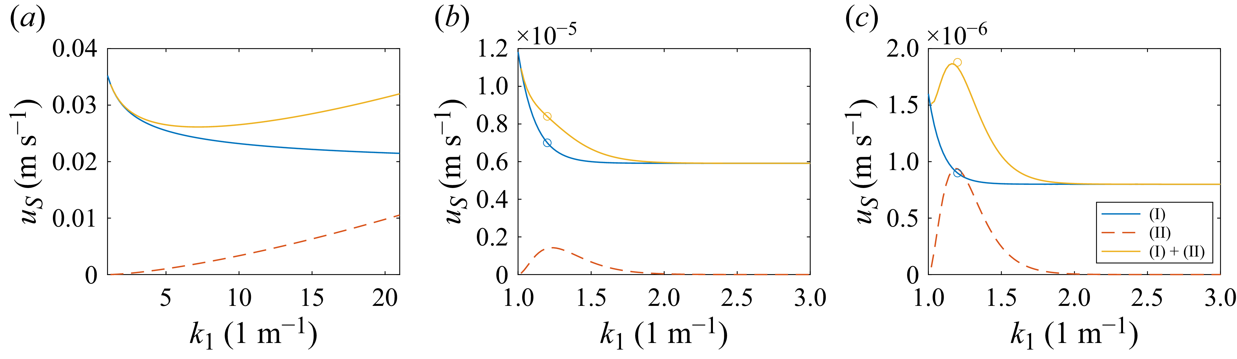


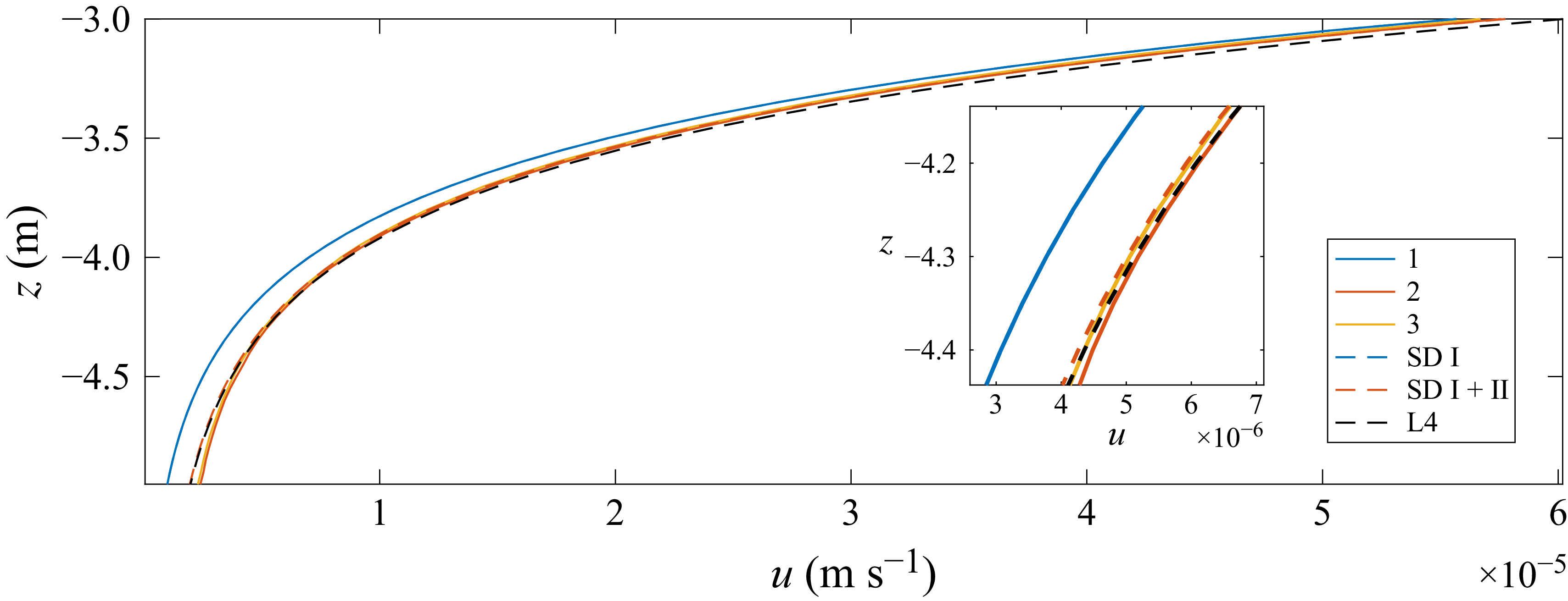


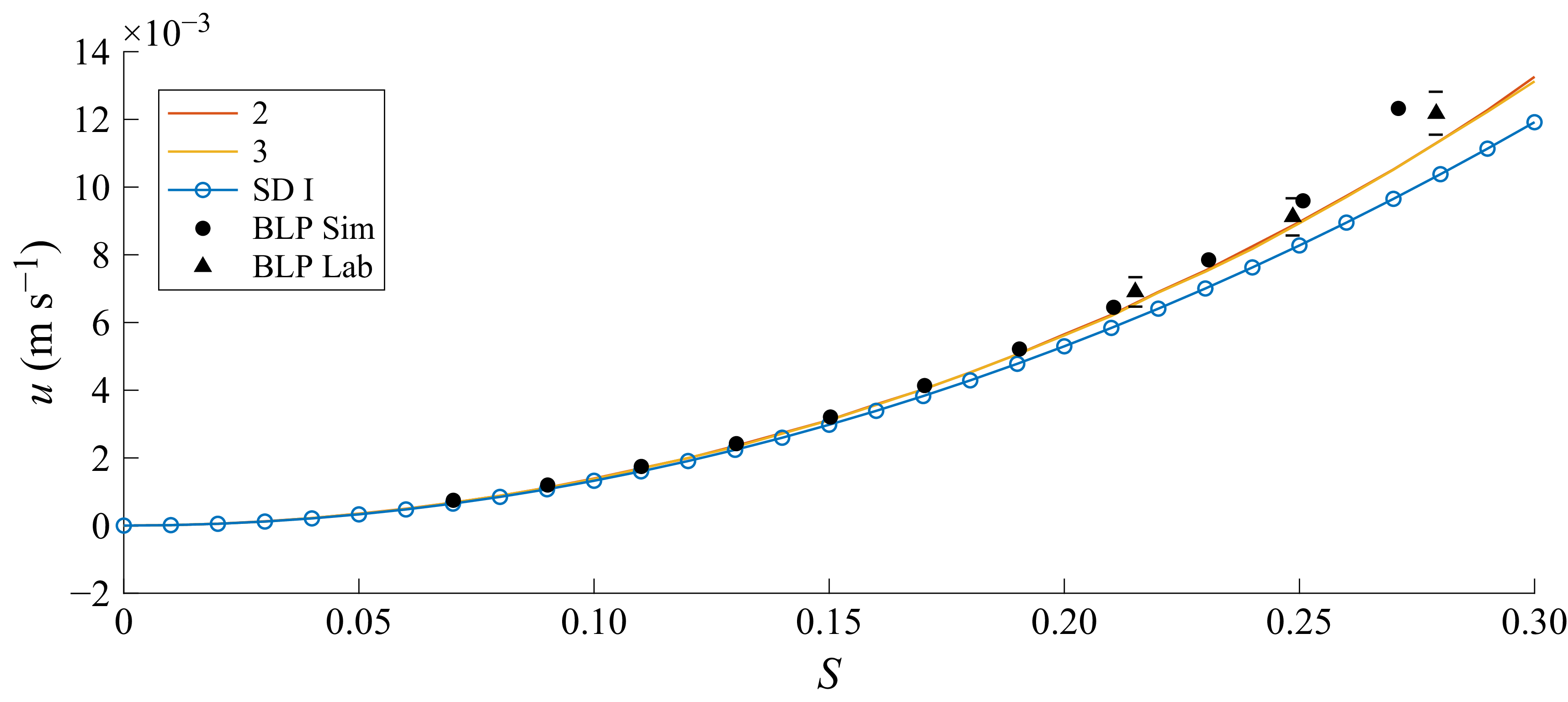


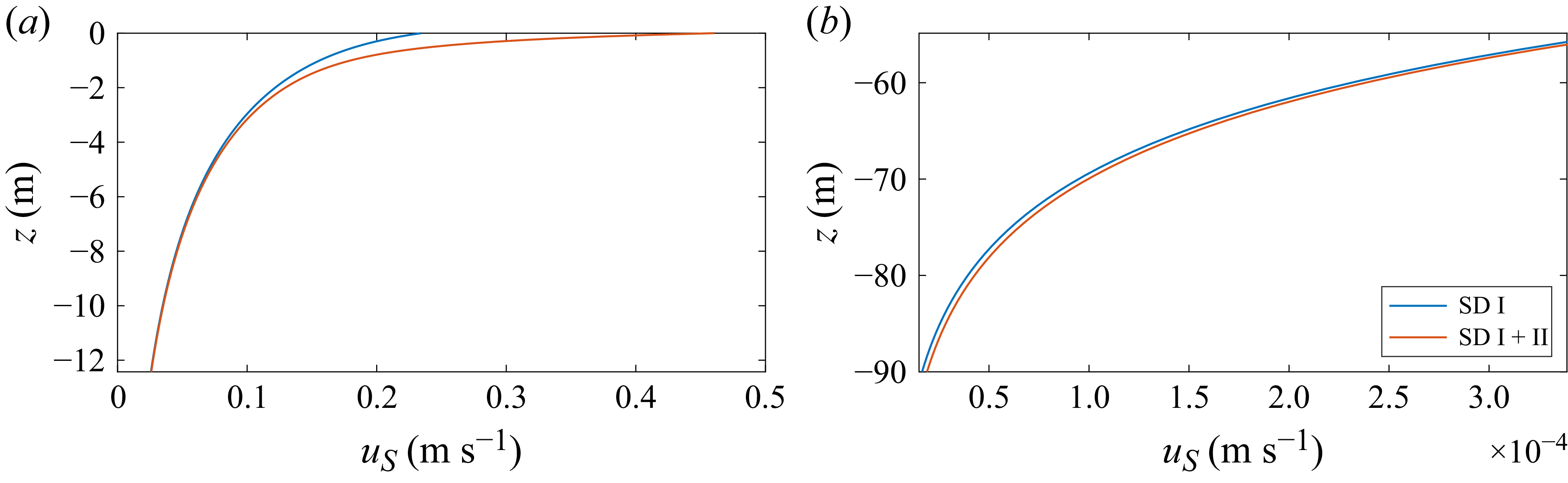


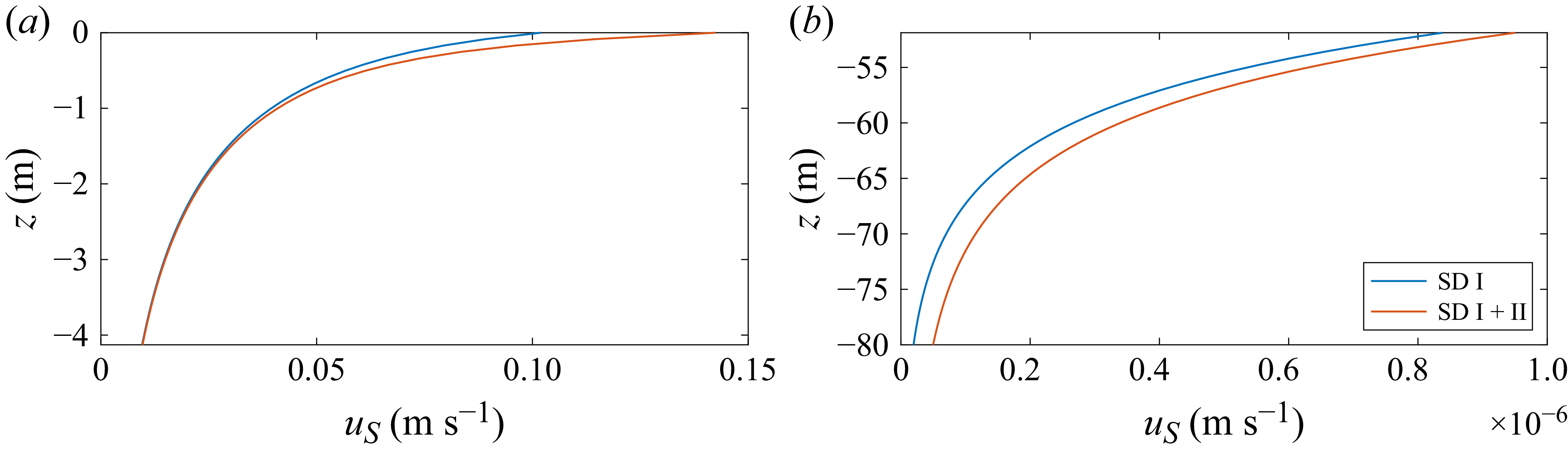


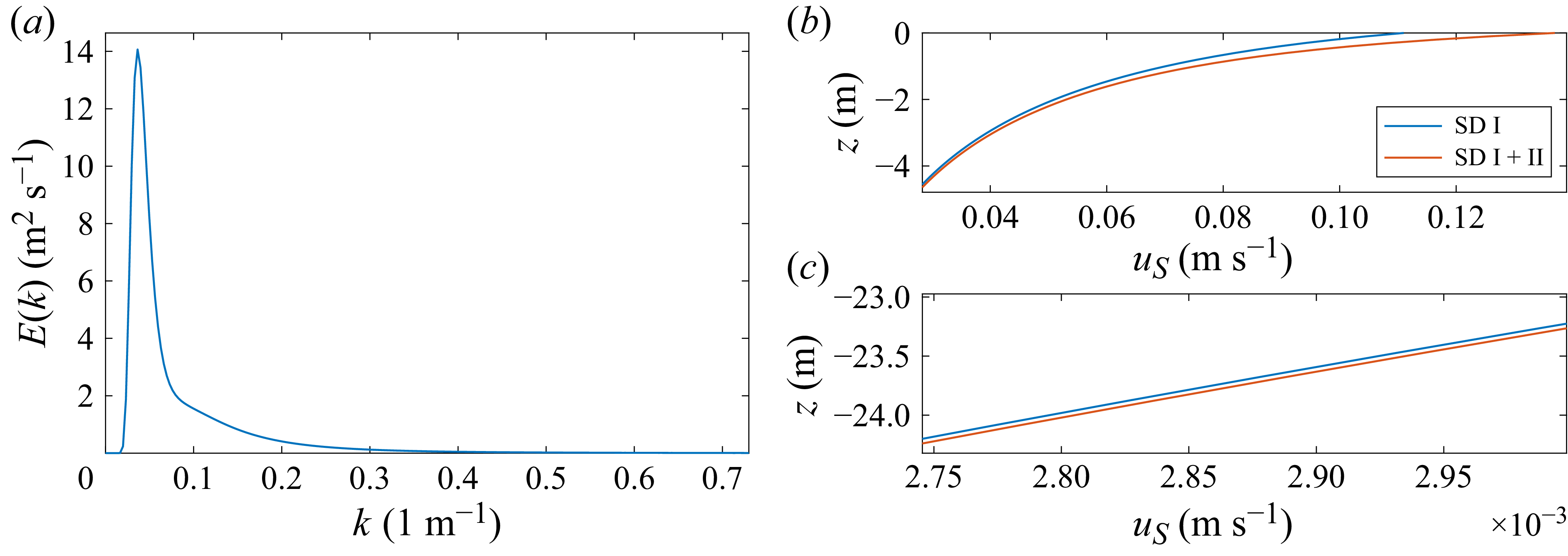


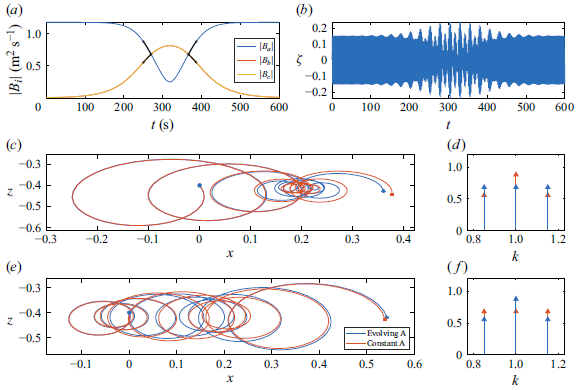


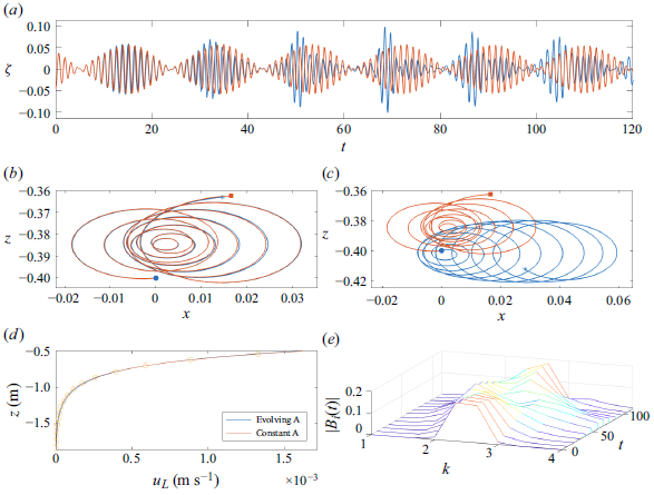


 Open access