


1. Introduction
Gravity currents are flows driven by natural convection, where gravity acts on a density gradient within a fluid (Huppert Reference Huppert2006; Wells & Dorrell Reference Wells and Dorrell2021). These buoyancy-driven flows are ubiquitous in both industrial and environmental settings, where gradients in fluid density may arise due to spatial variation in temperature, or in the concentration of suspended particulate or solute material.
Environmental gravity currents are often large-scale events that may cause significant hazards to both human life and structures. Naturally occurring examples include pyroclastic flows, powder-snow avalanches and turbidity currents. Pyroclastic flows, dense surface currents consisting of volcanic material and interstitial air, pose some of the most significant geohazard risks following a volcanic eruption. This is due to the high temperatures and speeds with which they propagate, often over 30 m s−1 and 500 $^\circ$
C, with a current thickness typically of the order of hundreds of metres (Wilson Reference Wilson2008). Powder-snow avalanches are a widely known form of gravity current on the Earth’s surface. They are driven by the suspension of snow particles, with air forming the interstitial fluid (Hopfinger Reference Hopfinger1983). Turbidity currents are ocean-floor sedimentary gravity currents that can run-out for thousands of kilometres along the ocean floor. Their deposits can host important natural resources (Reece, Dorrell & Straub Reference Reece, Dorrell and Straub2024). They travel with depth-averaged velocities of 0.1–6.6 m s−1, a current thickness of 95–135 m, and may pose a threat to ocean floor infrastructure such as pipelines and telecommunication cables (Meiburg & Kneller Reference Meiburg and Kneller2010; Peakall & Sumner Reference Peakall and Sumner2015; Wells & Dorrell Reference Wells and Dorrell2021).
$^\circ$
C, with a current thickness typically of the order of hundreds of metres (Wilson Reference Wilson2008). Powder-snow avalanches are a widely known form of gravity current on the Earth’s surface. They are driven by the suspension of snow particles, with air forming the interstitial fluid (Hopfinger Reference Hopfinger1983). Turbidity currents are ocean-floor sedimentary gravity currents that can run-out for thousands of kilometres along the ocean floor. Their deposits can host important natural resources (Reece, Dorrell & Straub Reference Reece, Dorrell and Straub2024). They travel with depth-averaged velocities of 0.1–6.6 m s−1, a current thickness of 95–135 m, and may pose a threat to ocean floor infrastructure such as pipelines and telecommunication cables (Meiburg & Kneller Reference Meiburg and Kneller2010; Peakall & Sumner Reference Peakall and Sumner2015; Wells & Dorrell Reference Wells and Dorrell2021).
The current and ambient fluid have initial densities of $\rho _{{0}}$
and
$\rho _{{0}}$
and $\rho _{{a}}$
, respectively. The system has a reduced gravity
$\rho _{{a}}$
, respectively. The system has a reduced gravity $g'=g(\rho _{{0}}-\rho _{{a}})/\rho _{{a}}$
, where
$g'=g(\rho _{{0}}-\rho _{{a}})/\rho _{{a}}$
, where $g$
is the acceleration due to gravity. When
$g$
is the acceleration due to gravity. When $(\rho _{{0}}-\rho _{{a}})/\rho _{{a}}\ll 1$
the current can be modelled using the Boussinesq approximation, where density variations within the fluid are neglected in the governing equations unless they are acted on by gravity (Meiburg & Kneller Reference Meiburg and Kneller2010; Tritton Reference Tritton2012; Fukuda et al. Reference Fukuda2023). Non-Boussinesq flows are beyond the scope of the present study.
$(\rho _{{0}}-\rho _{{a}})/\rho _{{a}}\ll 1$
the current can be modelled using the Boussinesq approximation, where density variations within the fluid are neglected in the governing equations unless they are acted on by gravity (Meiburg & Kneller Reference Meiburg and Kneller2010; Tritton Reference Tritton2012; Fukuda et al. Reference Fukuda2023). Non-Boussinesq flows are beyond the scope of the present study.
Environmental gravity currents are challenging to observe directly due to their large scale, infrequent and destructive nature. The dynamics of dilute currents are studied using theoretical, experimental and numerical modelling. Quantifying and predicting front propagation speeds is of particular interest when studying the dynamics of gravity currents. Canonical idealised models consider a ‘lock-gate’ release of a denser than ambient fluid (Huppert & Simpson Reference Huppert and Simpson1980; Rottman & Simpson Reference Rottman and Simpson1983; Hogg Reference Hogg2006; Meiburg, Radhakrishnan & Nasr-Azadani Reference Meiburg, Radhakrishnan and Nasr-Azadani2015). Such models consist of a straight channel with a gate, separating a relatively dense fluid of concentration $\rho _{{0}}$
, from a lighter ambient fluid of concentration
$\rho _{{0}}$
, from a lighter ambient fluid of concentration $\rho _{{a}}\lt \rho _{{0}}$
. When the gate is removed a horizontal hydrostatic pressure gradient is created, which induces a gravity current to propagate along the channel (Huppert & Simpson Reference Huppert and Simpson1980; Andrews & Manga Reference Andrews and Manga2012). The characteristic length scale in the vertical and horizontal directions are taken to be the initial current depth
$\rho _{{a}}\lt \rho _{{0}}$
. When the gate is removed a horizontal hydrostatic pressure gradient is created, which induces a gravity current to propagate along the channel (Huppert & Simpson Reference Huppert and Simpson1980; Andrews & Manga Reference Andrews and Manga2012). The characteristic length scale in the vertical and horizontal directions are taken to be the initial current depth $h_{{0}}$
, and lock length
$h_{{0}}$
, and lock length $x_{{0}}$
, respectively. The buoyancy velocity,
$x_{{0}}$
, respectively. The buoyancy velocity, $U_{{b}}=\sqrt {g'h_{{0}}}$
, is the characteristic velocity scale. The non-dimensional parameters that govern the dynamics of the lock-exchange gravity current are the buoyancy Reynolds number,
$U_{{b}}=\sqrt {g'h_{{0}}}$
, is the characteristic velocity scale. The non-dimensional parameters that govern the dynamics of the lock-exchange gravity current are the buoyancy Reynolds number,
 \begin{equation} \textit{Re}_{{b}}=(U_{{b}} h_{{0}})/(\nu ), \end{equation}
and Schmidt number,
 \begin{equation} \textit{Sc}=\nu /D; \end{equation}
where $\nu$
is the kinematic viscosity of the ambient fluid, and
$\nu$
is the kinematic viscosity of the ambient fluid, and $D$
is the diffusivity of the scalar concentration field.
$D$
is the diffusivity of the scalar concentration field.
Following a brief acceleration phase, gravity currents transition through three distinct phases: slumping, inertial and viscous (Huppert & Simpson Reference Huppert and Simpson1980). In the slumping phase the current propagates at a constant velocity referred to as the buoyancy Froude number, $\textit{Fr}_{{b}}=u_{\!{f}}/U_{{b}}$
, under a balance of pressure and drag forces. The inertial phase is governed by a balance of inertial and buoyancy forces, where front location scales like
$\textit{Fr}_{{b}}=u_{\!{f}}/U_{{b}}$
, under a balance of pressure and drag forces. The inertial phase is governed by a balance of inertial and buoyancy forces, where front location scales like $x_{\!{f}}\propto t^{({2}/{3})}$
(Fay Reference Fay1971; Hoult Reference Hoult1972; Huppert & Simpson Reference Huppert and Simpson1980; Hogg Reference Hogg2006; Cantero et al. Reference Cantero, Lee, Balachandar and Garcia2007). The viscous phase is governed by a balance of viscous and buoyancy forces, where front location scales like
$x_{\!{f}}\propto t^{({2}/{3})}$
(Fay Reference Fay1971; Hoult Reference Hoult1972; Huppert & Simpson Reference Huppert and Simpson1980; Hogg Reference Hogg2006; Cantero et al. Reference Cantero, Lee, Balachandar and Garcia2007). The viscous phase is governed by a balance of viscous and buoyancy forces, where front location scales like $x_{\!{f}}\propto t^{({1}/{5})}$
(Hoult Reference Hoult1972; Huppert Reference Huppert1982; Cantero et al. Reference Cantero, Lee, Balachandar and Garcia2007).
$x_{\!{f}}\propto t^{({1}/{5})}$
(Hoult Reference Hoult1972; Huppert Reference Huppert1982; Cantero et al. Reference Cantero, Lee, Balachandar and Garcia2007).
Standard lock-exchange experiments model an environmental flow in which a finite volume of dense fluid is instantaneously released. However, in naturally occurring currents dense material is often released in successive stages, generating pulsed currents. Pulsed flows have various potential causes, including temporal variation in seismic activity, retrogressive slope failure and the confluence of two gravity current flows (Mulder & Alexander Reference Mulder and Alexander2001; Beeson, Johnson & Goldfinger Reference Beeson, Johnson and Goldfinger2017; Goldfinger et al. Reference Goldfinger, Galer, Beeson, Hamilton, Black, Romsos, Patton, Nelson, Hausmann and Morey2017; Johnson et al. Reference Johnson, Gomberg, Hautala and Salmi2017). The geological record at the Cascadia margin, Washington, USA, provides evidence of deposits formed by the merging of turbidity currents at multiple channel confluences (Goldfinger et al. Reference Goldfinger, Galer, Beeson, Hamilton, Black, Romsos, Patton, Nelson, Hausmann and Morey2017).
The pyroclastic flow generated by the Soufrière Hills Volcano eruption in 1997 contained three distinct current releases. However, hazard assessments assumed a single release (Loughlin et al. Reference Loughlin, Calder, Clarke, Cole, Luckett, Mangan, Pyle, Sparks, Voight and Watts2002). Using the details documented by Loughlin et al. (Reference Loughlin, Calder, Clarke, Cole, Luckett, Mangan, Pyle, Sparks, Voight and Watts2002) we can estimate the non-dimensional delay time between the first and second pulse. Loughlin et al. (Reference Loughlin, Calder, Clarke, Cole, Luckett, Mangan, Pyle, Sparks, Voight and Watts2002) states that the current eruption was associated with three seismic events, which occurred at times 12:57:15 ( $\pm \, 20 \,\mathrm{s}$
), 12:59:55 (
$\pm \, 20 \,\mathrm{s}$
), 12:59:55 ( $\pm \, 30 \,\mathrm{s}$
) and 13:08:20 (
$\pm \, 30 \,\mathrm{s}$
) and 13:08:20 ( $\pm \, 30 \,\mathrm{s}$
). The first and second pulse were therefore separated by 110–210 s. Loughlin et al. (Reference Loughlin, Calder, Clarke, Cole, Luckett, Mangan, Pyle, Sparks, Voight and Watts2002) reports a reference density for the current of
$\pm \, 30 \,\mathrm{s}$
). The first and second pulse were therefore separated by 110–210 s. Loughlin et al. (Reference Loughlin, Calder, Clarke, Cole, Luckett, Mangan, Pyle, Sparks, Voight and Watts2002) reports a reference density for the current of $1.6\:\mathrm{kg\,m}^{-3}$
, and we assume ambient air is at standard temperature and pressure (
$1.6\:\mathrm{kg\,m}^{-3}$
, and we assume ambient air is at standard temperature and pressure ( $1.29\:\mathrm{kg\,m}^{-3}$
). Given these values we have a reduced gravity of
$1.29\:\mathrm{kg\,m}^{-3}$
). Given these values we have a reduced gravity of $g' = 2.36\:\mathrm{m\,s}^{-2}$
. Finally, we must assign a characteristic length scale for the system as Loughlin et al. (Reference Loughlin, Calder, Clarke, Cole, Luckett, Mangan, Pyle, Sparks, Voight and Watts2002) does not estimate the initial flow depth. We take the length scale to be in the range
$g' = 2.36\:\mathrm{m\,s}^{-2}$
. Finally, we must assign a characteristic length scale for the system as Loughlin et al. (Reference Loughlin, Calder, Clarke, Cole, Luckett, Mangan, Pyle, Sparks, Voight and Watts2002) does not estimate the initial flow depth. We take the length scale to be in the range $[500, 1000]\,\mathrm{m}$
, as this is the order of magnitude of the flow depth of pyroclastic currents (Jones et al. Reference Jones, Beckett, Bernard, Breard, Dioguardi, Dufek, Engwell and Eychenne2023). A length scale of
$[500, 1000]\,\mathrm{m}$
, as this is the order of magnitude of the flow depth of pyroclastic currents (Jones et al. Reference Jones, Beckett, Bernard, Breard, Dioguardi, Dufek, Engwell and Eychenne2023). A length scale of $500\,\mathrm{m}$
results in a buoyancy velocity of
$500\,\mathrm{m}$
results in a buoyancy velocity of $U_{\textit{b}} = 34.3\:\mathrm{m\,s}^{-1}$
, and a non-dimensional time delay between the first and second pulse in the range
$U_{\textit{b}} = 34.3\:\mathrm{m\,s}^{-1}$
, and a non-dimensional time delay between the first and second pulse in the range $[7.55, 14.42]$
, accounting for uncertainty in the release times. Taking a length scale of
$[7.55, 14.42]$
, accounting for uncertainty in the release times. Taking a length scale of $1000\,\mathrm{m}$
results in a buoyancy velocity scale of
$1000\,\mathrm{m}$
results in a buoyancy velocity scale of $U_{\textit{b}} = 48.55\:\mathrm{m\,s}^{-1}$
, and a non-dimensional time delay between the first and second pulse in the range
$U_{\textit{b}} = 48.55\:\mathrm{m\,s}^{-1}$
, and a non-dimensional time delay between the first and second pulse in the range $[5.34, 10.20]$
. We investigate the dynamics of pulsed currents using an idealised experiment to allow careful study of the impact on front propagation relative to an instantaneous release for a wide range of non-dimensional delay times between pulses. Here, for simplicity, we use conservative flows as a proxy for non-conservative depositional flows (Meiburg et al. Reference Meiburg, Radhakrishnan and Nasr-Azadani2015).
$[5.34, 10.20]$
. We investigate the dynamics of pulsed currents using an idealised experiment to allow careful study of the impact on front propagation relative to an instantaneous release for a wide range of non-dimensional delay times between pulses. Here, for simplicity, we use conservative flows as a proxy for non-conservative depositional flows (Meiburg et al. Reference Meiburg, Radhakrishnan and Nasr-Azadani2015).
There have been limited studies on pulsed gravity currents. Ho et al. (Reference Ho, Dorrell, Keevil, Burns and McCaffrey2018a
) conducted lock-exchange experiments where two locks of length $x_{{0}}$
were released successively, with a non-dimensional delay time of
$x_{{0}}$
were released successively, with a non-dimensional delay time of $\tilde {t}_{\textit{re}} = (t_{\textit{re}} U_{\textit{b}})/x_0$
separating the release of the first and second lock, where
$\tilde {t}_{\textit{re}} = (t_{\textit{re}} U_{\textit{b}})/x_0$
separating the release of the first and second lock, where $t_{\textit{re}}$
is the dimensional delay time. The results showed the second current propagated as an intrusion into the first and ultimately the pulses merged to form a unified front, as can be observed in the visualisations of the experiments presented in figure 1. Ho et al. (Reference Ho, Dorrell, Keevil, Burns and McCaffrey2018a
) also considered the implications for sedimentary deposits in turbidity currents, which was explored further by Ho et al. (Reference Ho, Dorrell, Keevil, Thomas, Burns, Baas and McCaffrey2019). Ho et al. (Reference Ho, Dorrell, Keevil, Burns and McCaffrey2018b
) conducted an analysis of the length scales of pulse merging. The pulsed gravity problem has similarities to the two-layer stratified locks, in that two gravity currents interact and mix over the lifetime of the flow (Dai Reference Dai2017; Zhu, He & Meiburg Reference Zhu, He and Meiburg2023).
$t_{\textit{re}}$
is the dimensional delay time. The results showed the second current propagated as an intrusion into the first and ultimately the pulses merged to form a unified front, as can be observed in the visualisations of the experiments presented in figure 1. Ho et al. (Reference Ho, Dorrell, Keevil, Burns and McCaffrey2018a
) also considered the implications for sedimentary deposits in turbidity currents, which was explored further by Ho et al. (Reference Ho, Dorrell, Keevil, Thomas, Burns, Baas and McCaffrey2019). Ho et al. (Reference Ho, Dorrell, Keevil, Burns and McCaffrey2018b
) conducted an analysis of the length scales of pulse merging. The pulsed gravity problem has similarities to the two-layer stratified locks, in that two gravity currents interact and mix over the lifetime of the flow (Dai Reference Dai2017; Zhu, He & Meiburg Reference Zhu, He and Meiburg2023).
Visualisation of a sequential lock-box gravity current release (Ho et al. Reference Ho, Dorrell, Keevil, Burns and McCaffrey2018a
). In the experiments the lock-box length $x_{{0}}=0.125\:\mathrm{m}$
, the initial current depth
$x_{{0}}=0.125\:\mathrm{m}$
, the initial current depth $h_{{0}}=0.05\:\mathrm{m}$
, the second lock was released at
$h_{{0}}=0.05\:\mathrm{m}$
, the second lock was released at $t_{\textit{re}}=4\:\mathrm{s}$
and the buoyancy velocity scale
$t_{\textit{re}}=4\:\mathrm{s}$
and the buoyancy velocity scale $U_{{b}}=0.1566\:\mathrm{m}\,\mathrm{s}^{-1}$
. Time is non-dimensionalised as
$U_{{b}}=0.1566\:\mathrm{m}\,\mathrm{s}^{-1}$
. Time is non-dimensionalised as $\tilde {t}=(t U_{{b}})/x_{{0}}$
, resulting in a non-dimensional release time of
$\tilde {t}=(t U_{{b}})/x_{{0}}$
, resulting in a non-dimensional release time of $\tilde {t}_{\textit{re}}=5$
.
$\tilde {t}_{\textit{re}}=5$
.

Methods used to numerically model idealised lock-gate releases can broadly be divided into two categories: depth-averaged models based on the shallow-water equations (SWEs) (Dorrell et al. Reference Dorrell, Darby, Peakall, Sumner, Parsons and Wynn2014), and depth-resolving models based on the Navier–Stokes equations (Marshall et al. Reference Marshall, Dorrell, Dutta, Keevil, Peakall and Tobias2021). Numerical simulations of pulsed gravity currents were conducted by Allen et al. (Reference Allen, Dorrell, Harlen, Thomas and McCaffrey2020), where the authors applied a depth-averaged SWE model to simulate the flow generated by a pulsed lock-exchange experiment, and explored pulsed flows for different regimes of $\tilde {t}_{\textit{re}}$
. Allen et al. (Reference Allen, Dorrell, Harlen, Thomas and McCaffrey2020) showed that as
$\tilde {t}_{\textit{re}}$
. Allen et al. (Reference Allen, Dorrell, Harlen, Thomas and McCaffrey2020) showed that as $\tilde {t}_{\textit{re}}\to \infty$
the pulses propagate as separate currents, and for
$\tilde {t}_{\textit{re}}\to \infty$
the pulses propagate as separate currents, and for $\tilde {t}_{\textit{re}}\lt 1$
flow is equivalent to a single stage release of twice the volume, as the backwards travelling wave has yet to impact the second lock. For intermediate values of
$\tilde {t}_{\textit{re}}\lt 1$
flow is equivalent to a single stage release of twice the volume, as the backwards travelling wave has yet to impact the second lock. For intermediate values of $\tilde {t}_{\textit{re}}$
, the second pulse advanced more rapidly than the first and ultimately merged with it, in agreement with the experimental findings. Allen et al. (Reference Allen, Dorrell, Harlen, Thomas and McCaffrey2020) also observed that the speed of the second current at the time of merging was positively correlated with the delay time between releases. However, Allen et al. (Reference Allen, Dorrell, Harlen, Thomas and McCaffrey2020) terminated simulations at the time of pulse merging. The front propagation of pulsed gravity currents after the currents merge, as a function of
$\tilde {t}_{\textit{re}}$
, the second pulse advanced more rapidly than the first and ultimately merged with it, in agreement with the experimental findings. Allen et al. (Reference Allen, Dorrell, Harlen, Thomas and McCaffrey2020) also observed that the speed of the second current at the time of merging was positively correlated with the delay time between releases. However, Allen et al. (Reference Allen, Dorrell, Harlen, Thomas and McCaffrey2020) terminated simulations at the time of pulse merging. The front propagation of pulsed gravity currents after the currents merge, as a function of $\tilde {t}_{\textit{re}}$
, has not been studied.
$\tilde {t}_{\textit{re}}$
, has not been studied.
The present study aims to address this open research question using the results of pulsed lock-exchange physical experiments, in combination with depth-averaged and depth-resolving numerical models. The research objectives are to investigate the front propagation of pulsed currents as a function of $\tilde {t}_{\textit{re}}$
and elucidate the underlying dynamics.
$\tilde {t}_{\textit{re}}$
and elucidate the underlying dynamics.
2. Methods
The dynamics of pulsed gravity currents are investigated using physical experiments and numerical simulations, where the simulations include both depth-averaging and depth-resolving numerical models. We consider the dual-stage release lock-exchange problem. A schematic of the problem set-up and key parameters are presented in figure 2. The set-up consists of a straight channel of length $L_{{1}}$
, width
$L_{{1}}$
, width $L_{{2}}$
and height
$L_{{2}}$
and height $L_{{3}}$
. The channel contains two locks, each retaining a saline mixture of density
$L_{{3}}$
. The channel contains two locks, each retaining a saline mixture of density $\rho _{{0}}$
, separated from ambient fluid of density
$\rho _{{0}}$
, separated from ambient fluid of density $\rho _{{a}}$
. The density difference between the saline mixture and ambient fluid is small,
$\rho _{{a}}$
. The density difference between the saline mixture and ambient fluid is small, $(\rho _{{0}}-\rho _{{a}})/\rho _{{a}}\ll 1$
, hence the Boussinesq approximation can be applied. The initial depth of dense fluid is
$(\rho _{{0}}-\rho _{{a}})/\rho _{{a}}\ll 1$
, hence the Boussinesq approximation can be applied. The initial depth of dense fluid is $h_{{0}}$
, with the remaining channel depth (
$h_{{0}}$
, with the remaining channel depth ( $L_3-h_{{0}}$
) containing ambient fluid. Both locks have a length of
$L_3-h_{{0}}$
) containing ambient fluid. Both locks have a length of $x_{{0}}$
. The gates are released successively, with a delay time of
$x_{{0}}$
. The gates are released successively, with a delay time of $\tilde {t}_{\textit{re}}=({ t_{\textit{re}} U_{{b}} }/{x_{{0}}})$
between the release of the first and second lock. The front location of the pulses generated by the first and second release are
$\tilde {t}_{\textit{re}}=({ t_{\textit{re}} U_{{b}} }/{x_{{0}}})$
between the release of the first and second lock. The front location of the pulses generated by the first and second release are $x_{\!{f}}^1$
and
$x_{\!{f}}^1$
and $x_{\!{f}}^2$
, respectively.
$x_{\!{f}}^2$
, respectively.
Schematic of dual-stage lock-exchange experiment.

Case parameters for the dual-stage release lock-exchange study. The parameter space was investigated using a combination of physical experiments (Exp), depth-averaged SWE simulations and depth-resolving LBM simulations as indicated in the table.

Thirty-three physical and numerical experiments quantifying dual-stage release flows are considered, the parameters for each case are presented in table 1. The physical experiments were conducted at a buoyancy Reynolds number of $\textit{Re}_{{b}} \approx 6000$
. The case list includes fractional depths of release of
$\textit{Re}_{{b}} \approx 6000$
. The case list includes fractional depths of release of $h_{{0}}/L_{{3}} \in {\{10^{-5}, 0.1, 0.2, 0.5\}}$
. For each fractional depth of release we vary the non-dimensional delay time between the release of the first and second lock,
$h_{{0}}/L_{{3}} \in {\{10^{-5}, 0.1, 0.2, 0.5\}}$
. For each fractional depth of release we vary the non-dimensional delay time between the release of the first and second lock, $\tilde {t}_{\textit{re}}$
. As indicated in table 1, depth-averaged SWE simulations were conducted for Cases 1–27, physical experiments are run for Cases 13–18 and 25–27, and depth-resolving lattice Boltzmann method (LBM) simulations were run for Cases 25–33. The LBM simulations were run with a Reynolds number of
$\tilde {t}_{\textit{re}}$
. As indicated in table 1, depth-averaged SWE simulations were conducted for Cases 1–27, physical experiments are run for Cases 13–18 and 25–27, and depth-resolving lattice Boltzmann method (LBM) simulations were run for Cases 25–33. The LBM simulations were run with a Reynolds number of $\textit{Re}_{{b}}=6000$
. This allows the results of the physical experiments, SWE simulations and LBM simulations to be directly compared for Cases 25–27, where
$\textit{Re}_{{b}}=6000$
. This allows the results of the physical experiments, SWE simulations and LBM simulations to be directly compared for Cases 25–27, where $h_{{0}}/L_{{3}} = 0.5$
. We are able to explore a wider parameter space with the SWE model due to its low computational cost relative to the depth-resolving LBM simulations.
$h_{{0}}/L_{{3}} = 0.5$
. We are able to explore a wider parameter space with the SWE model due to its low computational cost relative to the depth-resolving LBM simulations.
2.1. Physical experiments
Physical experiments modelling pulsed-release lock-exchange gravity currents were conducted in a 5 m-long flume. At one end of the flume, two saline fluid regions of the same volume were contained in two lockboxes set up in series to model a pulsed current with two releases. The experimental set-up follows that of Ho et al. (Reference Ho, Dorrell, Keevil, Burns and McCaffrey2018a , Reference Ho, Dorrell, Keevil, Burns and McCaffrey2018b ) and Allen et al. (Reference Allen, Dorrell, Harlen, Thomas and McCaffrey2020). Fluid in the two lockboxes were dyed yellow and blue to enable the visualisation of current mixing. The timing between two lock gates was set to vary between 0 s and 21.2 s using a pneumatic lock control box that ensured repeatability of both the timing and the speed of withdrawal of the lock. The density excess of the saline was 5 %. The height of the initial saline fluids and the length of each lock box were 0.05 m and 0.125 m, respectively. Ambient heights were set at 0.1 m and 0.25 m. The evolution of flows was captured using two rail mounted high-definition cameras, tracking individual pulse fronts.
2.2. Numerical modelling
The macroscopic governing equations for a pulsed lock-exchange saline gravity current flow are those of mass and momentum conservation for an incompressible flow coupled, via the Boussinesq approximation, with an advection–diffusion equation for the scalar concentration field. Fluid density is defined as
 \begin{equation} \rho (\boldsymbol{x},t)=\rho _{{a}}(1+\alpha \chi (\boldsymbol{x},t)), \end{equation}
where $\alpha =(\rho _{{s}}-\rho _{{a}})/\rho _{{a}}$
,
$\alpha =(\rho _{{s}}-\rho _{{a}})/\rho _{{a}}$
, $\rho _{{s}}$
is solute density and
$\rho _{{s}}$
is solute density and $\chi (\boldsymbol{x},t)$
is solute concentration. The body force generated by the action of gravity is
$\chi (\boldsymbol{x},t)$
is solute concentration. The body force generated by the action of gravity is $\boldsymbol{G}$
,
$\boldsymbol{G}$
,
 \begin{equation} \boldsymbol{G}=-g\rho _{{a}}(1+\alpha \chi (\boldsymbol{x},t)) \hat {\boldsymbol{z}}, \end{equation}
where $\hat {\boldsymbol{z}}$
is the unit vector in the upward vertical direction.
$\hat {\boldsymbol{z}}$
is the unit vector in the upward vertical direction. $\boldsymbol{G}$
includes a constant term that is the hydrostatic pressure term in the momentum equation,
$\boldsymbol{G}$
includes a constant term that is the hydrostatic pressure term in the momentum equation, $\boldsymbol{\nabla \!} P= \boldsymbol{\nabla }(p_{{k}}(\boldsymbol{x},t))-g\rho _{{a}} z$
, where
$\boldsymbol{\nabla \!} P= \boldsymbol{\nabla }(p_{{k}}(\boldsymbol{x},t))-g\rho _{{a}} z$
, where $p_{{k}}$
is the kinematic pressure. The driving force is the Boussinesq forcing term
$p_{{k}}$
is the kinematic pressure. The driving force is the Boussinesq forcing term $\boldsymbol{F}_{\!\textit{B}}$
,
$\boldsymbol{F}_{\!\textit{B}}$
,
 \begin{equation} \boldsymbol{F}_{\!\textit{B}}=-g\rho _a\alpha \chi (\boldsymbol{x},t) \hat {\boldsymbol{z}}. \end{equation}
The governing equations are non-dimensionalised using the characteristic length scale $h_0=0.05$
m, and velocity scale
$h_0=0.05$
m, and velocity scale $U_{\textit{b}}=0.1566$
m s−1, resulting in the non-dimensional incompressible mass and momentum conservation equations,
$U_{\textit{b}}=0.1566$
m s−1, resulting in the non-dimensional incompressible mass and momentum conservation equations,
 \begin{equation} \boldsymbol{\nabla }\boldsymbol{\cdot }\tilde {\boldsymbol{u}}=0, \end{equation}
 \begin{equation} \frac {\partial \tilde {\boldsymbol{u}}}{\partial \tilde {t}} + \tilde {\boldsymbol{u}} \boldsymbol{\cdot }\boldsymbol{\tilde {\boldsymbol{\nabla }}} \tilde {\boldsymbol{u}} = -\boldsymbol{\tilde {\boldsymbol{\nabla }}}\tilde {P} + \frac {1}{\textit{Re}_b} \tilde {{\nabla} }^2 \tilde {\boldsymbol{u}} - \tilde {\chi } \hat {\boldsymbol{z}} \end{equation}
and an advection–diffusion equation for the scalar concentration field $\tilde {\chi }$
,
$\tilde {\chi }$
,
 \begin{equation} \frac {\partial \tilde {\chi }}{\partial \tilde {t}} + \tilde {\boldsymbol{u}} \boldsymbol{\cdot }\boldsymbol{\tilde {\boldsymbol{\nabla }}} \tilde {\chi } = \frac {1}{\textit{Re}_b Sc} \tilde {{\nabla} }^2 \tilde {\chi }. \end{equation}
In addition to the buoyancy Reynolds number ( $\textit{Re}_{{b}}$
) the governing equations are also parameterised by the Schmidt number
$\textit{Re}_{{b}}$
) the governing equations are also parameterised by the Schmidt number $Sc= ({\nu }/{D})$
, where
$Sc= ({\nu }/{D})$
, where $D$
is the diffusivity of the scalar field. All simulations are run with
$D$
is the diffusivity of the scalar field. All simulations are run with $Sc=1$
. The Schmidt number of real-world flows may be orders of magnitude larger, but the structure and dynamics of Boussinesq currents are relatively insensitive to Schmidt number for high Reynolds numbers of
$Sc=1$
. The Schmidt number of real-world flows may be orders of magnitude larger, but the structure and dynamics of Boussinesq currents are relatively insensitive to Schmidt number for high Reynolds numbers of $\mathcal{O}(10^4)$
(Bonometti & Balachandar Reference Bonometti and Balachandar2008; Marshall et al. Reference Marshall, Dorrell, Dutta, Keevil, Peakall and Tobias2021).
$\mathcal{O}(10^4)$
(Bonometti & Balachandar Reference Bonometti and Balachandar2008; Marshall et al. Reference Marshall, Dorrell, Dutta, Keevil, Peakall and Tobias2021).
The concentration field is scaled relative to the initial saline concentration in the lock $\chi _{{0}}$
, i.e.
$\chi _{{0}}$
, i.e. $\tilde {\chi },(\boldsymbol{x},t)=\chi (\boldsymbol{x},t)/\chi _{{0}}$
. Fluid density is non-dimensionalised using the initial density of the current and ambient, such that
$\tilde {\chi },(\boldsymbol{x},t)=\chi (\boldsymbol{x},t)/\chi _{{0}}$
. Fluid density is non-dimensionalised using the initial density of the current and ambient, such that $\tilde {\rho }(\boldsymbol{x},t) = (\rho (\boldsymbol{x},t) - \rho _{{a}})/(\rho _{{0}}-\rho _{{a}})$
. Variables with a
$\tilde {\rho }(\boldsymbol{x},t) = (\rho (\boldsymbol{x},t) - \rho _{{a}})/(\rho _{{0}}-\rho _{{a}})$
. Variables with a $\tilde{}$
accent are non-dimensionalised, and variables with a
$\tilde{}$
accent are non-dimensionalised, and variables with a $\bar {}$
accent are the spanwise average of a non-dimensionalised variable, i.e.
$\bar {}$
accent are the spanwise average of a non-dimensionalised variable, i.e.
 \begin{equation} \bar {\rho }(\tilde {x},\tilde {z},\tilde {t})=\frac {1}{\tilde {L}_2}\int \limits _{0}^{\tilde {L}_2}\tilde {\rho }(\tilde {x},\tilde {y},\tilde {z},\tilde {t})\,\mathrm{d}\tilde {y}. \end{equation}
Here the macroscopic governing equations are not solved directly. We compare the use of: a depth-averaged model, implemented using the shallow-water approximation (§ 2.2.1); and a depth-resolving model, solving the governing equations at a mesoscopic scale, using a LBM model (§ 2.2.2).
2.2.1. Depth-averaged shallow-water equations model
In this section the methodology for an analytical SWE model is presented. Shallow-water models have extensively been used to study the lock-exchange problem as they exploit the small ratio between depth and length scales $ \delta \sim h_{{f}}/x^1_{{f}}$
. Consider a two-layered flow of immiscible fluids of thicknesses
$ \delta \sim h_{{f}}/x^1_{{f}}$
. Consider a two-layered flow of immiscible fluids of thicknesses $h_1(x,t)$
and
$h_1(x,t)$
and $h_2(x,t)$
and of similar, but distinct densities
$h_2(x,t)$
and of similar, but distinct densities $\rho _{{a}}$
and
$\rho _{{a}}$
and $\rho _{{0}}$
, respectively, with
$\rho _{{0}}$
, respectively, with $\rho _{{a}}\lt \rho _{{0}}$
, figure 3. The flow is assumed to be symmetric in the cross-stream (
$\rho _{{a}}\lt \rho _{{0}}$
, figure 3. The flow is assumed to be symmetric in the cross-stream ( $y$
-direction) and the flow properties only vary over the direction of propagation
$y$
-direction) and the flow properties only vary over the direction of propagation $x$
. Further, by assuming that the flows are inviscid, the depths
$x$
. Further, by assuming that the flows are inviscid, the depths $h_i$
and depth-averaged velocities
$h_i$
and depth-averaged velocities $u_i$
for each layer are functions of
$u_i$
for each layer are functions of $(x,t)$
only. Surface tension and other intermolecular forces are assumed to be negligible. With the rigid-lid assumption total depth is
$(x,t)$
only. Surface tension and other intermolecular forces are assumed to be negligible. With the rigid-lid assumption total depth is $\mathcal{H}(x,t)=h_1+h_2 = L_3$
and the the two-layer shallow-water model that was formulated by Rottman & Simpson (Reference Rottman and Simpson1983) can be applied. Using
$\mathcal{H}(x,t)=h_1+h_2 = L_3$
and the the two-layer shallow-water model that was formulated by Rottman & Simpson (Reference Rottman and Simpson1983) can be applied. Using $l_{{0}}$
as the length scale,
$l_{{0}}$
as the length scale, $h_{{0}}$
as our depth scale,
$h_{{0}}$
as our depth scale, $\sqrt {h_{{0}}g'}$
as the velocity scale and the convective time scale
$\sqrt {h_{{0}}g'}$
as the velocity scale and the convective time scale $\sqrt {h_{{0}}/g'}$
, the dimensionless equations two-layer shallow-water equations are
$\sqrt {h_{{0}}/g'}$
, the dimensionless equations two-layer shallow-water equations are
 \begin{align} \frac {\partial \tilde {h}}{\partial \tilde {t}}+\frac {\partial \tilde {m}}{\partial \tilde {x}}&=0,\\[-12pt]\nonumber \end{align}
 \begin{align} \frac {\partial \tilde {m}}{\partial \tilde {t}}+\frac {\tilde {m}}{\tilde {h}}(2-2a)\frac {\partial \tilde {m}}{\partial \tilde {x}} -\left (\frac {\tilde {m}^2}{\tilde {h}^2}(1-2a)-\tilde {h}(1-b)\right )\frac {\partial \tilde {h}}{\partial \tilde {x}}&=0, \\[9pt] \nonumber \end{align}
where
 \begin{align} a &= \frac {\tilde {h}}{\tilde {L}_3-\tilde {h}}, \end{align}
 \begin{align} b &= \frac {\tilde {h}}{\tilde {L}_3} + \frac {\tilde {m}^2}{\tilde {L}_3\tilde {h}^2}\left (1-\frac {\tilde {h}}{\tilde {L}_3}\right )^{-2}\!. \\[9pt] \nonumber \end{align}
Double lock-release configuration for the shallow-water model: before the second gate release, (a) $\tilde {t}\lt \tilde {t}_{\textit{re}}$
, and after the second gate release, (b)
$\tilde {t}\lt \tilde {t}_{\textit{re}}$
, and after the second gate release, (b) $\tilde {t}\gt \tilde {t}_{\textit{re}}$
. The second release creates a shock in the solution which propagates forwards towards the head of the current. Horizontal and vertical lengths are non-dimensionalised by the lock-length
$\tilde {t}\gt \tilde {t}_{\textit{re}}$
. The second release creates a shock in the solution which propagates forwards towards the head of the current. Horizontal and vertical lengths are non-dimensionalised by the lock-length $l_{\textit{lock}}$
and lock depth
$l_{\textit{lock}}$
and lock depth $h_{\text{0}}$
, respectively. The position of the head is labelled
$h_{\text{0}}$
, respectively. The position of the head is labelled $\tilde {x}^1_{{f}}$
and the second release that appears as a shock
$\tilde {x}^1_{{f}}$
and the second release that appears as a shock $\tilde {x}^2_{{f}}$
.
$\tilde {x}^2_{{f}}$
.

Note that in the infinitely deep ambient limit, $\tilde {L}_3\to \infty$
and
$\tilde {L}_3\to \infty$
and $a,b\to 0$
, the single-layer equations are recovered (Ungarish & Zemach Reference Ungarish and Zemach2005; Ungarish Reference Ungarish2009). For flows in relatively deep
$a,b\to 0$
, the single-layer equations are recovered (Ungarish & Zemach Reference Ungarish and Zemach2005; Ungarish Reference Ungarish2009). For flows in relatively deep $\tilde {L}_3\gg 1$
, the standard shallow-water equations can still be used and flow in the ambient neglected (Rottman & Simpson Reference Rottman and Simpson1983; Hogg, Ungarish & Huppert Reference Hogg, Ungarish and Huppert2000; Hogg Reference Hogg2006; Allen et al. Reference Allen, Dorrell, Harlen, Thomas and McCaffrey2020). However, as the ambient depth
$\tilde {L}_3\gg 1$
, the standard shallow-water equations can still be used and flow in the ambient neglected (Rottman & Simpson Reference Rottman and Simpson1983; Hogg, Ungarish & Huppert Reference Hogg, Ungarish and Huppert2000; Hogg Reference Hogg2006; Allen et al. Reference Allen, Dorrell, Harlen, Thomas and McCaffrey2020). However, as the ambient depth $\tilde {L}_3$
decreases the propagation speed of characteristic curves reduces, which leads to quantitative differences in the solution for lock-exchange gravity currents. For example, the duration of the slumping phase (where the head moves at constant speed) is increased (Rottman & Simpson Reference Rottman and Simpson1983). The influence on the flow dynamics of the finite ambient depth increases as
$\tilde {L}_3$
decreases the propagation speed of characteristic curves reduces, which leads to quantitative differences in the solution for lock-exchange gravity currents. For example, the duration of the slumping phase (where the head moves at constant speed) is increased (Rottman & Simpson Reference Rottman and Simpson1983). The influence on the flow dynamics of the finite ambient depth increases as $\tilde {L}_3$
decreases until
$\tilde {L}_3$
decreases until $\tilde {L}_3\lt 2$
, where the formation of a backwards propagating shock causes qualitative differences in the solution (Klemp, Rotunno & Skamarock Reference Klemp, Rotunno and Skamarock1994; Ungarish & Zemach Reference Ungarish and Zemach2005). The changing dynamics as
$\tilde {L}_3\lt 2$
, where the formation of a backwards propagating shock causes qualitative differences in the solution (Klemp, Rotunno & Skamarock Reference Klemp, Rotunno and Skamarock1994; Ungarish & Zemach Reference Ungarish and Zemach2005). The changing dynamics as $\tilde {L}_3$
decreases arise because of the increased work done by current accelerating the ambient fluid as it moves.
$\tilde {L}_3$
decreases arise because of the increased work done by current accelerating the ambient fluid as it moves.
The initial and boundary conditions reflect a double lock-release and are equivalent to those used in Allen et al. (Reference Allen, Dorrell, Harlen, Thomas and McCaffrey2020) to study dual-stage releases gravity currents in a infinitely deep ambient,
 \begin{align} \tilde {h}(\tilde {x},0) =& \begin{cases} 1 \quad & \text{if} \quad \tilde {x}\in [0,2],\\ 0 \quad & \text{otherwise}, \end{cases} \end{align}
 \begin{align} \tilde {u}(\tilde {x},0) =& 0, \end{align}
 \begin{align} \frac {\partial \tilde {h}}{\partial \tilde {x}}(\tilde {x}_0,\tilde {t}) =& 0 \quad \text{for}\quad \begin{cases} \tilde {x}_0 = 0 ,1 \quad &\text{for}\quad 0\leqslant \tilde {t} \lt \tilde {t}_{\textit{re}},\\ \tilde {x}_0 = 0 \quad &\text{for} \quad \tilde {t} \gt \tilde {t}_{\textit{re}}, \end{cases} \end{align}
where $\tilde {t}_{\textit{re}}$
is the release time of the second lock box.
$\tilde {t}_{\textit{re}}$
is the release time of the second lock box.
As discussed in the introduction, the moving head of the gravity current (right-hand boundary in this configuration) requires supplementation with a Froude number condition to accurately predict the propagation dynamics. The Froude number condition is expressed as a relationship between the depth $\tilde{h}_{\kern-1pt f}$
and velocity
$\tilde{h}_{\kern-1pt f}$
and velocity $\tilde {u}_{{f}}$
at the head of the flow
$\tilde {u}_{{f}}$
at the head of the flow $\tilde {x}=\tilde {x}_{{f}}^1(t)$
. At the head of the flow the dynamic boundary condition is also imposed giving
$\tilde {x}=\tilde {x}_{{f}}^1(t)$
. At the head of the flow the dynamic boundary condition is also imposed giving
 \begin{equation} \frac {{\textrm{d}} \tilde {x}^1_{{f}}}{{\textrm{d}} \tilde {t}}\equiv \dot {\tilde {x}}^1_{{f}} = \tilde {u}\left(\tilde {x}=\tilde {x}^1_{{f}},t \right) = \textit{Fr} \sqrt {\tilde{h}_{\kern-1pt f}}, \end{equation}
where $\tilde{h}_{\kern-1pt f}(\tilde {t}) = \tilde {h}(\tilde {x}=\tilde {x}^1_{{f}},\tilde {t})$
. In general the Froude number is a decreasing function of
$\tilde{h}_{\kern-1pt f}(\tilde {t}) = \tilde {h}(\tilde {x}=\tilde {x}^1_{{f}},\tilde {t})$
. In general the Froude number is a decreasing function of $\tilde{h}_{\kern-1pt f}/\tilde {L}_3$
and many experimental or analytical expression exist for it (Benjamin (Reference Benjamin1968), Huppert & Simpson (Reference Huppert and Simpson1980), Rottman & Simpson (Reference Rottman and Simpson1983)). As
$\tilde{h}_{\kern-1pt f}/\tilde {L}_3$
and many experimental or analytical expression exist for it (Benjamin (Reference Benjamin1968), Huppert & Simpson (Reference Huppert and Simpson1980), Rottman & Simpson (Reference Rottman and Simpson1983)). As $\tilde {L}_3\to \infty$
, the Froude number tends to a constant value and for deep ambient flows a constant value is taken (Hogg Reference Hogg2006; Allen et al. Reference Allen, Dorrell, Harlen, Thomas and McCaffrey2020). Ungarish & Zemach (Reference Ungarish and Zemach2005) present a semiempirical formulation,
$\tilde {L}_3\to \infty$
, the Froude number tends to a constant value and for deep ambient flows a constant value is taken (Hogg Reference Hogg2006; Allen et al. Reference Allen, Dorrell, Harlen, Thomas and McCaffrey2020). Ungarish & Zemach (Reference Ungarish and Zemach2005) present a semiempirical formulation,
 \begin{equation} \textit{Fr} \left (\frac {\tilde{h}_{\kern-1pt f}}{\tilde {L}_3}\right ) = \textit{Fr}_{\textit{u}z}\left (\frac {\tilde {h}_{\!{f}}}{\tilde {L}_3}\right ) \left (1+3\frac {\tilde {h}_{\!{f}}}{\tilde {L}_3}\right )^{-1/2}\!, \end{equation}
as a compromise between other correlations whilst maintaining a reasonable agreement with a variety of experimental results. Crucially, the difference between these expressions is not particularly large in the region of shallow-water solutions $h_{\!{f}}/\tilde {L}_3 \lt 0.6$
(Ungarish & Zemach Reference Ungarish and Zemach2005). The present study is limited to the ranges
$h_{\!{f}}/\tilde {L}_3 \lt 0.6$
(Ungarish & Zemach Reference Ungarish and Zemach2005). The present study is limited to the ranges $\tilde {L}_3\geqslant 2$
, or
$\tilde {L}_3\geqslant 2$
, or $\tilde {h}_{\!{f}}/\tilde {L}_3 \lt 0.5$
. As
$\tilde {h}_{\!{f}}/\tilde {L}_3 \lt 0.5$
. As $\tilde {L}_3\to \infty$
,
$\tilde {L}_3\to \infty$
, $\textit{Fr}_{\textit{u}z}\to 1$
. In addition to simulations conducted with
$\textit{Fr}_{\textit{u}z}\to 1$
. In addition to simulations conducted with $\textit{Fr}=\textit{Fr}_{\textit{u}z}$
, constant values of the Froude number
$\textit{Fr}=\textit{Fr}_{\textit{u}z}$
, constant values of the Froude number $ \textit{Fr} $
are also used for simulations with an infinitely deep ambient
$ \textit{Fr} $
are also used for simulations with an infinitely deep ambient $\tilde {L}_3\to \infty$
.
$\tilde {L}_3\to \infty$
.
To numerically solve the two-layer shallow-water model, ((2.8) and (2.9)) are mapped onto the unit interval $[0,1]$
using the transformation
$[0,1]$
using the transformation $ (\zeta ,\tau )= (\tilde {x}/\tilde {x}^1_{{f}},\tilde {t} )$
. These scaled equations are solved using a Lax–Wendroff finite difference method similar to Bonnecaze, Huppert & Lister (Reference Bonnecaze, Huppert and Lister1993), Ungarish & Zemach (Reference Ungarish and Zemach2005) and Allen et al. (Reference Allen, Dorrell, Harlen, Thomas and McCaffrey2020). A small artificial viscosity term is introduced using the formulation presented in Ungarish & Zemach (Reference Ungarish and Zemach2005) to remove spurious oscillations that arise near large gradients and prevent the chequerboarding instability that arises with the Lax–Wendroff. For further details see Appendix A.
$ (\zeta ,\tau )= (\tilde {x}/\tilde {x}^1_{{f}},\tilde {t} )$
. These scaled equations are solved using a Lax–Wendroff finite difference method similar to Bonnecaze, Huppert & Lister (Reference Bonnecaze, Huppert and Lister1993), Ungarish & Zemach (Reference Ungarish and Zemach2005) and Allen et al. (Reference Allen, Dorrell, Harlen, Thomas and McCaffrey2020). A small artificial viscosity term is introduced using the formulation presented in Ungarish & Zemach (Reference Ungarish and Zemach2005) to remove spurious oscillations that arise near large gradients and prevent the chequerboarding instability that arises with the Lax–Wendroff. For further details see Appendix A.
2.2.2. Depth-resolving LBM model
Depth-resolving simulations are produced by solving the macroscopic governing equations at the mesoscopic scale, i.e. between the macroscopic and microscopic scales, using the LBM (Krüger et al. Reference Krüger, Kusumaatmaja, Kuzmin, Shardt, Silva and Viggen2017). The LBM simulations are run in VirtualFluids, an open-source graphics processing unit accelerated code developed by the Institute for Computational Modelling in Civil Engineering (iRMB) at TU Braunschweig. Adekanye et al. (Reference Adekanye, Khan, Burns, McCaffrey, Geier, Schönherr and Dorrell2022) validated VirtualFluids for the simulation of instantaneous release lock-exchange gravity currents with Reynolds numbers up to $\textit{Re}_{{b}}=30\,000$
, showing good agreement with high-resolution simulations and physical experiments.
$\textit{Re}_{{b}}=30\,000$
, showing good agreement with high-resolution simulations and physical experiments.
At the mesoscopic scale fluid motion is described by the particle distribution function (PDF) $f(\boldsymbol{x},\boldsymbol{\xi }, t)$
, where
$f(\boldsymbol{x},\boldsymbol{\xi }, t)$
, where $\boldsymbol{\xi }$
is particle velocity. The PDF defines the density of particles at location
$\boldsymbol{\xi }$
is particle velocity. The PDF defines the density of particles at location $\boldsymbol{x}$
, moving with velocity
$\boldsymbol{x}$
, moving with velocity $\boldsymbol{\xi }$
, at time
$\boldsymbol{\xi }$
, at time $t$
. The evolution of
$t$
. The evolution of $f(\boldsymbol{x},\boldsymbol{\xi }, t)$
is governed by the Boltzmann equation, which when discretised in space and time produces the lattice Boltzmann equation. In the present study we solve two two-way coupled lattice Boltzmann equations, one for the conservation of mass and momentum in the fluid,
$f(\boldsymbol{x},\boldsymbol{\xi }, t)$
is governed by the Boltzmann equation, which when discretised in space and time produces the lattice Boltzmann equation. In the present study we solve two two-way coupled lattice Boltzmann equations, one for the conservation of mass and momentum in the fluid,
 \begin{equation} f_{\textit{ijk}}(\boldsymbol{x} + \boldsymbol{\xi }_{\textit{ijk}}\Delta t, t + \Delta t) = f_{\textit{ijk}}(\boldsymbol{x}, t) + \varOmega ^f_{\textit{ijk}}(f_{\textit{ijk}}, \varPhi _{\textit{ijk}}), \end{equation}
and a second for the advection and diffusion of the scalar concentration field,
 \begin{equation} \varPhi _{\textit{ijk}}(\boldsymbol{x} + \boldsymbol{\xi }_{\textit{ijk}}\Delta t, t + \Delta t) = \varPhi _{\textit{ijk}}(\boldsymbol{x}, t) + \varOmega ^\varPhi _{\textit{ijk}}(\varPhi _{\textit{ijk}}, f_{\textit{ijk}}). \end{equation}
Solving the system of lattice Boltzmann equations for the PDFs $f_{\textit{ijk}}$
and
$f_{\textit{ijk}}$
and $\varPhi _{\textit{ijk}}$
is equivalent to to solving the macroscopic governing equations, (2.4)–(2.6) (Junk, Klar & Luo Reference Junk, Klar and Luo2004; Dubois Reference Dubois2008). The equations are coupled via their respective collision operators,
$\varPhi _{\textit{ijk}}$
is equivalent to to solving the macroscopic governing equations, (2.4)–(2.6) (Junk, Klar & Luo Reference Junk, Klar and Luo2004; Dubois Reference Dubois2008). The equations are coupled via their respective collision operators, $\varOmega ^f_{\textit{ijk}}$
and
$\varOmega ^f_{\textit{ijk}}$
and $\varOmega ^\varPhi _{\textit{ijk}}$
.
$\varOmega ^\varPhi _{\textit{ijk}}$
.
The discretised PDF $f_{\textit{ijk}}(\boldsymbol{x}, t)$
, is defined at the nodes of a lattice structure in which lattice nodes are connected by a discrete velocity set
$f_{\textit{ijk}}(\boldsymbol{x}, t)$
, is defined at the nodes of a lattice structure in which lattice nodes are connected by a discrete velocity set $\boldsymbol{\xi }_{\textit{ijk}}$
. The indices
$\boldsymbol{\xi }_{\textit{ijk}}$
. The indices $i,j,k$
are permutations of the values
$i,j,k$
are permutations of the values $\{1, 0, -1\}$
, and so
$\{1, 0, -1\}$
, and so $\boldsymbol{\xi }_{\textit{ijk}}$
is a set of vectors to neighbouring nodes, which includes the zero vector. In the present study a
$\boldsymbol{\xi }_{\textit{ijk}}$
is a set of vectors to neighbouring nodes, which includes the zero vector. In the present study a $D3Q27$
lattice is used, which results in the lattice structure presented in figure 4. In effect, distributions are constrained to stream along the vectors
$D3Q27$
lattice is used, which results in the lattice structure presented in figure 4. In effect, distributions are constrained to stream along the vectors $\boldsymbol{\xi }_{\textit{ijk}}$
in time
$\boldsymbol{\xi }_{\textit{ijk}}$
in time $\Delta t$
, where they collide and are redistributed according to the collision operator
$\Delta t$
, where they collide and are redistributed according to the collision operator $\varOmega _{\textit{ijk}}$
. The raw moments of a distribution, of order
$\varOmega _{\textit{ijk}}$
. The raw moments of a distribution, of order $\alpha +\beta +\gamma$
, are defined as
$\alpha +\beta +\gamma$
, are defined as
 \begin{equation} m_{\alpha \beta \gamma }(\theta _{\textit{ijk}})=\sum _{i,j,k} i^\alpha j^\beta k^\gamma \theta _{\textit{ijk}}. \end{equation}
The $D3Q27$
lattice structure.
$D3Q27$
lattice structure.

The macroscopic fluid density and momentum density are recovered from the zeroth and first-order raw moments of $f_{\textit{ijk}}$
,
$f_{\textit{ijk}}$
,
 \begin{align} \rho = m_{000}=\sum _{i,j,k}f_{\textit{ijk}}, \\[-29pt] \nonumber \end{align}
 \begin{align} \rho \boldsymbol{u} = \rho (m_{100},m_{010},m_{001}=\left ( \sum _{i,j,k}i \kern-1pt f_{\textit{ijk}}+\frac {\Delta t}{2}F_B^x , \sum _{i,j,k}j \kern-1pt f_{\textit{ijk}}+\frac {\Delta t}{2}F_B^y, \sum _{i,j,k}k f_{\textit{ijk}}+\frac {\Delta t}{2}F_B^z \right )\!. \\[-2pt] \nonumber \end{align}
The zeroth raw moment of the $\varPhi _{\textit{ijk}}$
distribution gives the macroscopic concentration,
$\varPhi _{\textit{ijk}}$
distribution gives the macroscopic concentration,
 \begin{equation} \chi = m_{000}=\sum _{i,j,k}\varPhi _{\textit{ijk}}. \end{equation}
Collisions for the $f_{\textit{ijk}}$
distribution are performed in cumulant space (Geier et al. Reference Geier, Schönherr, Pasquali and Krafczyk2015). Cumulants,
$f_{\textit{ijk}}$
distribution are performed in cumulant space (Geier et al. Reference Geier, Schönherr, Pasquali and Krafczyk2015). Cumulants, $C_{\textit{nrs}}$
, are relaxed towards their equilibria
$C_{\textit{nrs}}$
, are relaxed towards their equilibria $C_{\textit{nrs}}^{\textit{eq}}$
, at a rate
$C_{\textit{nrs}}^{\textit{eq}}$
, at a rate $\omega _{\textit{nrs}}$
,
$\omega _{\textit{nrs}}$
,
 \begin{equation} C_{\textit{nrs}}^*=(1-\omega _{\textit{nrs}})C_{\textit{nrs}} + \omega _{\textit{nrs}} C_{\textit{nrs}}^{\textit{eq}}. \end{equation}
The relaxation rate of the second-order cumulants determine the macroscopic fluid viscosity,
 \begin{equation} \nu =\frac {1}{3}\left (\frac {1}{\omega _{110}}-\frac {1}{2}\right )\frac {\Delta x^2}{\Delta t}. \end{equation}
Collisions for the $\varPhi _{\textit{ijk}}$
distribution are conducted in central moment space, using the method presented by Yang et al. (Reference Yang, Mehmani, Perkins, Pasquali, Schönherr, Kim, Perego, Parks, Trask and Balhoff2016). The factorised central moments
$\varPhi _{\textit{ijk}}$
distribution are conducted in central moment space, using the method presented by Yang et al. (Reference Yang, Mehmani, Perkins, Pasquali, Schönherr, Kim, Perego, Parks, Trask and Balhoff2016). The factorised central moments $M_{\textit{nrs}}$
are relaxed towards zero at the rate
$M_{\textit{nrs}}$
are relaxed towards zero at the rate $\omega _{\textit{nrs}}$
,
$\omega _{\textit{nrs}}$
,
 \begin{equation} M_{\textit{nrs}}^*=(1-\omega _{\textit{nrs}})M_{\textit{nrs}}. \end{equation}
The diffusivity of the scalar field is determined by the relaxation rate of the first-order factorised central moments,
 \begin{equation} D=\frac {1}{3}\left (\frac {1}{\omega _{100}}-\frac {1}{2}\right )\frac {\Delta x^2}{\Delta t}. \end{equation}
The dimensions of the computational domain are chosen to reflect the experimental conditions, with $L_1=27x_{{0}}$
, and
$L_1=27x_{{0}}$
, and $L_2=h_{{0}}$
, resulting in a non-dimensional domain size of
$L_2=h_{{0}}$
, resulting in a non-dimensional domain size of $\tilde {L}_1=27$
,
$\tilde {L}_1=27$
, $\tilde {L}_2=1$
,
$\tilde {L}_2=1$
, $\tilde {L}_3=L_3/h_0$
. Simulations are run on uniform meshes, with a spatial and time discretisation of
$\tilde {L}_3=L_3/h_0$
. Simulations are run on uniform meshes, with a spatial and time discretisation of $\Delta \tilde {x}={\Delta x}/{h_{{0}}}=0.01$
and
$\Delta \tilde {x}={\Delta x}/{h_{{0}}}=0.01$
and $\Delta \tilde {t}=3\times 10^{-4}$
, respectively. The grid resolution is chosen such that the largest length scales of turbulent motion are directly resolved, whilst stability is maintained by limiting the relaxation rate of the third-order cumulant, as specified in the parameterised cumulant method of Geier, Pasquali & Schönherr (Reference Geier, Pasquali and Schönherr2017).
$\Delta \tilde {t}=3\times 10^{-4}$
, respectively. The grid resolution is chosen such that the largest length scales of turbulent motion are directly resolved, whilst stability is maintained by limiting the relaxation rate of the third-order cumulant, as specified in the parameterised cumulant method of Geier, Pasquali & Schönherr (Reference Geier, Pasquali and Schönherr2017).
No-slip boundary conditions for the velocity field, and no-flux boundary conditions for the concentration field are applied to all external boundaries of the computational domain. These boundary conditions model the experimental set-up of the standard lock-exchange gravity current experiment, enabling direct validation against the observed front locations in the experimental results of Ho et al. (Reference Ho, Dorrell, Keevil, Burns and McCaffrey2018a ).
The specific conditions for the $\tilde {x}_{{B}}$
boundary are defined as
$\tilde {x}_{{B}}$
boundary are defined as
 \begin{align} \begin{aligned} \tilde {\boldsymbol{u}}(\tilde {\boldsymbol{x}}=(\tilde {x}_{\!{B}}, \tilde {y}, \tilde {z}), \tilde {t}) =&\ \boldsymbol{0}\\ \frac {\partial \tilde {\chi }}{\partial \tilde {x}}(\tilde {\boldsymbol{x}}=(\tilde {x}_{\!{B}}, \tilde {y}, \tilde {z}), \tilde {t}) =&\ 0 \end{aligned} \quad \text{for}\quad \begin{cases} \tilde {x}_{\!{B}} = 0 \lor \tilde {x}_0 \lor \tilde {L}_1 \quad &\text{for}\quad 0\leqslant \tilde {t} \lt \tilde {t}_{\textit{re}}\\ \tilde {x}_{\!{B}} = 0 \lor \tilde {L}_1 \quad &\text{for} \quad \tilde {t} \geqslant \tilde {t}_{\textit{re}} \end{cases}. \end{align}
A dual-stage release is achieved by inserting a no-slip and no-flux boundary condition on the $yz$
-plane at
$yz$
-plane at $\tilde {x}=\tilde {x}_0$
, which remains in effect until
$\tilde {x}=\tilde {x}_0$
, which remains in effect until $\tilde {t}=\tilde {t}_{\textit{re}}$
, as shown in (2.27). The removal of this internal wall simulates the release of the second lock gate.
$\tilde {t}=\tilde {t}_{\textit{re}}$
, as shown in (2.27). The removal of this internal wall simulates the release of the second lock gate.
The no-slip and no-flux conditions for the $\tilde {y}_{{B}}$
and
$\tilde {y}_{{B}}$
and $\tilde {z}_{{B}}$
boundaries are defined as
$\tilde {z}_{{B}}$
boundaries are defined as
 \begin{align} \begin{aligned} \tilde {\boldsymbol{u}}(\tilde {\boldsymbol{x}}=(\tilde {x}, \tilde {y}_{\!{B}}, \tilde {z}), \tilde {t}) =&\ \boldsymbol{0}\\ \frac {\partial \tilde {\chi }}{\partial \tilde {y}}(\tilde {\boldsymbol{x}}=(\tilde {x}, \tilde {y}_{\!{B}}, \tilde {z}), \tilde {t}) =&\ 0 \end{aligned} \quad \text{for}\quad \tilde {y}_{\!{B}} = 0 \lor \tilde {L}_2,\end{align}
 \begin{align} \begin{aligned} \tilde {\boldsymbol{u}}(\tilde {\boldsymbol{x}}=(\tilde {x}, \tilde {y}, \tilde {z}_{{B}}), \tilde {t}) =&\ \boldsymbol{0}\\ \frac {\partial \tilde {\chi }}{\partial \tilde {z}}(\tilde {\boldsymbol{x}}=(\tilde {x}, \tilde {y}, \tilde {z}_{{B}}), \tilde {t}) =&\ 0 \end{aligned} \quad \text{for}\quad \tilde {z}_{{B}} = 0 \lor \tilde {L}_3. \end{align}
No-slip and no-flux boundary conditions are implemented using the bounce-back method (Krüger et al. Reference Krüger, Kusumaatmaja, Kuzmin, Shardt, Silva and Viggen2017).
The initial conditions of the computational domain are
 \begin{align} \tilde {\chi }(\tilde {\boldsymbol{x}}, \tilde {t}=0) =& \begin{cases} 1 \quad & \text{if} \quad \tilde {x}\leqslant 2\tilde {x}_0 \land \tilde {z}\leqslant \tilde {h}_0\\ 0 \quad & \text{otherwise} \end{cases}, \end{align}
 \begin{align} \tilde {\boldsymbol{u}}(\tilde {\boldsymbol{x}}, \tilde {t}=0) =& 0. \end{align}
These conditions align with the schematic of the dual-stage release experiment shown in figure 2. The initial and boundary conditions extend the methods used in Adekanye et al. (Reference Adekanye, Khan, Burns, McCaffrey, Geier, Schönherr and Dorrell2022) to multistage releases. Adekanye et al. (Reference Adekanye, Khan, Burns, McCaffrey, Geier, Schönherr and Dorrell2022) validate LBM models of single-stage releases against experimental data. Therefore, we expect that the initial and boundary conditions will provide sufficient accuracy to capture the dynamics of pulsed flows.
For the simulations of Cases 28–33 two passive scalars distributions are added to the simulation, $\varPhi _{\textit{ijk}}^{{P1}}$
and
$\varPhi _{\textit{ijk}}^{{P1}}$
and $\varPhi _{\textit{ijk}}^{{P2}}$
, which simulate the advection–diffusion of two scalar fields
$\varPhi _{\textit{ijk}}^{{P2}}$
, which simulate the advection–diffusion of two scalar fields $\tilde {\chi }^{{P1}}$
and
$\tilde {\chi }^{{P1}}$
and $\tilde {\chi }^{{P2}}$
. The passive scalars are used to track the propagation and mixing of each release of dense material separately. The boundary conditions applied to the advection–diffusion simulations for
$\tilde {\chi }^{{P2}}$
. The passive scalars are used to track the propagation and mixing of each release of dense material separately. The boundary conditions applied to the advection–diffusion simulations for $\tilde {\chi }^{{P1}}$
and
$\tilde {\chi }^{{P1}}$
and $\tilde {\chi }^{{P2}}$
are the same as those applied to the
$\tilde {\chi }^{{P2}}$
are the same as those applied to the $\tilde {\chi }$
scalar field in (2.27)–(2.29). The initial conditions for the passive scalar fields are defined such that
$\tilde {\chi }$
scalar field in (2.27)–(2.29). The initial conditions for the passive scalar fields are defined such that $\tilde {\chi }^{{P1}}=1$
in the first lock and is zero elsewhere, while
$\tilde {\chi }^{{P1}}=1$
in the first lock and is zero elsewhere, while $\tilde {\chi }^{{P2}}=1$
in the second lock and is zero elsewhere,
$\tilde {\chi }^{{P2}}=1$
in the second lock and is zero elsewhere,
 \begin{align} \tilde {\chi }^{{P1}}(\tilde {\boldsymbol{x}}, \tilde {t}=0) =& \begin{cases} 1 \quad & \text{if} \quad \tilde {x}\leqslant 2\tilde {x}_0 \land \tilde {x}\gt \tilde {x}_0 \land \tilde {z}\leqslant \tilde {h}_0\\ 0 \quad & \text{otherwise} \end{cases}, \end{align}
 \begin{align} \tilde {\chi }^{{P2}}(\tilde {\boldsymbol{x}}, \tilde {t}=0) =& \begin{cases} 1 \quad & \text{if} \quad \tilde {x}\leqslant \tilde {x}_0 \land \tilde {z}\leqslant \tilde {h}_0\\ 0 \quad & \text{otherwise} \end{cases}. \end{align}
The passive scalars track the mixing of both pulses and can be used to determine the provenance of dense material at any time after the release of the lock gates.
Both the $\varPhi _{\textit{ijk}}^{{P1}}$
and
$\varPhi _{\textit{ijk}}^{{P1}}$
and $\varPhi _{\textit{ijk}}^{{P2}}$
are one-way coupled to the
$\varPhi _{\textit{ijk}}^{{P2}}$
are one-way coupled to the $f_{\textit{ijk}}$
distribution, so they are advected by the numerically calculated flow. The passive scalar distributions are solved for in an identical fashion to the two-way coupled distribution
$f_{\textit{ijk}}$
distribution, so they are advected by the numerically calculated flow. The passive scalar distributions are solved for in an identical fashion to the two-way coupled distribution $\varPhi _{\textit{ijk}}$
, using (2.18). As the Peclet number (
$\varPhi _{\textit{ijk}}$
, using (2.18). As the Peclet number ( $ \textit{Pe}=\textit{Re}_{{b}} Sc$
) is large (
$ \textit{Pe}=\textit{Re}_{{b}} Sc$
) is large ( $\textit{Pe} \approx 6000$
), we assume the impact of the diffusion term in (2.6) is negligible, hence
$\textit{Pe} \approx 6000$
), we assume the impact of the diffusion term in (2.6) is negligible, hence $\tilde {\chi }(\boldsymbol{x},t)\approx\tilde {\chi }^{{P1}}(\boldsymbol{x},t)+\tilde {\chi }^{{P2}}(\boldsymbol{x},t)$
.
$\tilde {\chi }(\boldsymbol{x},t)\approx\tilde {\chi }^{{P1}}(\boldsymbol{x},t)+\tilde {\chi }^{{P2}}(\boldsymbol{x},t)$
.
3. Results
3.1. Physical experiments
The front location of the gravity currents in Cases 13–18 and Cases 25–27 are presented in figure 5(a) and figure 5(b), respectively. The lock-exchange currents in Cases 13–18 have a fractional depth of release of $h_0/L_3 =0.2$
and delay times
$h_0/L_3 =0.2$
and delay times $\tilde {t}_{\textit{re}} \in [0.25,42.61]$
. Cases 25–27 have a fractional depth of release of
$\tilde {t}_{\textit{re}} \in [0.25,42.61]$
. Cases 25–27 have a fractional depth of release of $h_0/L_3 =0.5$
and delay times
$h_0/L_3 =0.5$
and delay times $\tilde {t}_{\textit{re}} \in [0.21,10.15]$
. The solid curves in figure 5 correspond to the front location of the current produced by the release of the first lock-gate, while the dashed lines track the front of the second pulse. When the pulses merge the dashed curve merges with the solid curve from the merge time
$\tilde {t}_{\textit{re}} \in [0.21,10.15]$
. The solid curves in figure 5 correspond to the front location of the current produced by the release of the first lock-gate, while the dashed lines track the front of the second pulse. When the pulses merge the dashed curve merges with the solid curve from the merge time $\tilde {t}_{{M}}$
onwards. We observe a maximum variance in measured front location of
$\tilde {t}_{{M}}$
onwards. We observe a maximum variance in measured front location of $\sigma ^2=0.19x_0$
across four repeats of physical experiments of Case 13.
$\sigma ^2=0.19x_0$
across four repeats of physical experiments of Case 13.
(a) Plots of front location of first pulse ( $x_{\!{f}}^1$
) in physical experiments (Exp) for
$x_{\!{f}}^1$
) in physical experiments (Exp) for $h_0/L_3 =0.2$
, Cases 13–18. (b) Plots of front location of first pulse (
$h_0/L_3 =0.2$
, Cases 13–18. (b) Plots of front location of first pulse ( $x_{\!{f}}^1$
) in physical experiments for
$x_{\!{f}}^1$
) in physical experiments for $h_0/L_3 =0.5$
Cases 25–27. (c) Plots of front location in physical experiments of Cases 13–18 relative to Case 13 (
$h_0/L_3 =0.5$
Cases 25–27. (c) Plots of front location in physical experiments of Cases 13–18 relative to Case 13 ( $\Delta \tilde {x}^1_{{f}}$
). (d) Plots of front location in physical experiments of Cases 25–27 relative to Case 25 (
$\Delta \tilde {x}^1_{{f}}$
). (d) Plots of front location in physical experiments of Cases 25–27 relative to Case 25 ( $\Delta \tilde {x}^1_{{f}}$
). The solid curves correspond to the front location of the current produced by the release of the first lock-gate, while the dashed lines track the front of the second pulse.
$\Delta \tilde {x}^1_{{f}}$
). The solid curves correspond to the front location of the current produced by the release of the first lock-gate, while the dashed lines track the front of the second pulse.

The results for Cases 13 and 25, where $\tilde {t}_{\textit{re}}\approx 0$
, provide baselines against which to measure the impact of varying
$\tilde {t}_{\textit{re}}\approx 0$
, provide baselines against which to measure the impact of varying $\tilde {t}_{\textit{re}}$
. Cases 13 and 25 are single stage releases of a lock with dimensions
$\tilde {t}_{\textit{re}}$
. Cases 13 and 25 are single stage releases of a lock with dimensions $2\tilde {x}_0\times \tilde {h}_0$
. Within the slumping phase, where
$2\tilde {x}_0\times \tilde {h}_0$
. Within the slumping phase, where $\tilde {x}_{{f}}\propto \tilde {t}$
, the current propagates with a buoyancy Froude number
$\tilde {x}_{{f}}\propto \tilde {t}$
, the current propagates with a buoyancy Froude number $ (\textit{Fr}_{{b}}=u_{\!{f}}/U_{{b}} )$
of
$ (\textit{Fr}_{{b}}=u_{\!{f}}/U_{{b}} )$
of $\textit{Fr}_{{b}}=0.51$
in Case 13, and
$\textit{Fr}_{{b}}=0.51$
in Case 13, and $\textit{Fr}_{{b}}=0.55$
in Case 25. This value is calculated by taking the mean velocity of the front for
$\textit{Fr}_{{b}}=0.55$
in Case 25. This value is calculated by taking the mean velocity of the front for $\tilde {t}\leqslant 8$
. After exiting the slumping phase the single stage release currents transition through the inertial phase and into the viscous phase. This is demonstrated in figure 5(a,b), where we observe the the current front locations briefly scaling like
$\tilde {t}\leqslant 8$
. After exiting the slumping phase the single stage release currents transition through the inertial phase and into the viscous phase. This is demonstrated in figure 5(a,b), where we observe the the current front locations briefly scaling like $\bar {x}_{{f}} \propto \tilde {t}^{2/3}$
, before scaling like
$\bar {x}_{{f}} \propto \tilde {t}^{2/3}$
, before scaling like $\bar {x}_{{f}} \propto \tilde {t}^{1/5}$
at later times.
$\bar {x}_{{f}} \propto \tilde {t}^{1/5}$
at later times.
In Cases 14–18, where there is a delay between the release of the first and second lock, the current initially propagates as a single release of a lock with dimensions $\tilde {x}_0\times \tilde {h}_0$
. The release of the second lock gate generates a dense intrusion into the leading gravity current. The pulses ultimately merge to form a unified front, as seen in figure 1. The merging time corresponds to an inflection point in the solid curve tracking the front location of the leading current. This is due to the acceleration of the front relative to its velocity immediately prior to the time of merging. The same trends are observed in Cases 25–27, where Case 25 is the baseline case
$\tilde {x}_0\times \tilde {h}_0$
. The release of the second lock gate generates a dense intrusion into the leading gravity current. The pulses ultimately merge to form a unified front, as seen in figure 1. The merging time corresponds to an inflection point in the solid curve tracking the front location of the leading current. This is due to the acceleration of the front relative to its velocity immediately prior to the time of merging. The same trends are observed in Cases 25–27, where Case 25 is the baseline case $(\tilde {t}_{\textit{re}}=0.25)$
against which Cases 26 and 27 are compared. Although both lock gates in Cases 13 and 25 are released simultaneously, there is still a non-zero merging time due to the transit time for the downstream buoyancy-flux in the inner region of the body to transport dense material to the head of the current.
$(\tilde {t}_{\textit{re}}=0.25)$
against which Cases 26 and 27 are compared. Although both lock gates in Cases 13 and 25 are released simultaneously, there is still a non-zero merging time due to the transit time for the downstream buoyancy-flux in the inner region of the body to transport dense material to the head of the current.
The findings here are best illustrated through plots of the relative front location of each pulsed current $(\tilde {t}_{\textit{re}}\gt 0)$
compared with a single release of an equal volume of dense fluid, i.e. the
$(\tilde {t}_{\textit{re}}\gt 0)$
compared with a single release of an equal volume of dense fluid, i.e. the $\tilde {t}_{\textit{re}}\approx 0$
case with equivalent parameters. The relative displacement between the front of a single and pulsed release is defined as
$\tilde {t}_{\textit{re}}\approx 0$
case with equivalent parameters. The relative displacement between the front of a single and pulsed release is defined as
 \begin{equation} \Delta \tilde {x}^1_{{f}}(\tilde {t}, \tilde {t}_{\textit{re}}) = \tilde {x}^1_{{f}}(\tilde {t}, \tilde {t}_{\textit{re}}) - \tilde {x}^1_{{f}}(\tilde {t}, \tilde {t}_{\textit{re}}=0). \end{equation}
Plots of relative front location $(\Delta \tilde {x}^1_{{f}})$
against time are presented in figures 5(c) and 5(d) for Cases 13–18 and Cases 25–27, respectively. These are plots of front location in a frame of reference moving with the front of the single release currents.
$(\Delta \tilde {x}^1_{{f}})$
against time are presented in figures 5(c) and 5(d) for Cases 13–18 and Cases 25–27, respectively. These are plots of front location in a frame of reference moving with the front of the single release currents.
The same trends are observed in both sets of results. For the benchmark cases, Cases 13 and 25 where $\tilde {t}_{\textit{re}}\approx 0$
, the
$\tilde {t}_{\textit{re}}\approx 0$
, the $\Delta \tilde {x}^1_{{f}}$
curve is identically zero for all
$\Delta \tilde {x}^1_{{f}}$
curve is identically zero for all $\tilde {t}$
by definition. Several clear trends emerge when comparing the front position of pulsed currents with their respective benchmarks. At early times the relative front location is negative,
$\tilde {t}$
by definition. Several clear trends emerge when comparing the front position of pulsed currents with their respective benchmarks. At early times the relative front location is negative, $\Delta \tilde {x}^1_{{f}}\lt 0$
. This distance continues to grow until the merge time of each pulsed current. At the merge time there is an inflection point in the
$\Delta \tilde {x}^1_{{f}}\lt 0$
. This distance continues to grow until the merge time of each pulsed current. At the merge time there is an inflection point in the $\Delta \tilde {x}^1_{{f}}$
curves, and the unified fronts of the pulsed gravity currents accelerate relative to the front of the single release current. The relative acceleration of the pulsed flows does not continue indefinitely, ultimately the acceleration slows and the relative front position plateaus at a constant value. At late times the unified front propagates under the viscous scaling law,
$\Delta \tilde {x}^1_{{f}}$
curves, and the unified fronts of the pulsed gravity currents accelerate relative to the front of the single release current. The relative acceleration of the pulsed flows does not continue indefinitely, ultimately the acceleration slows and the relative front position plateaus at a constant value. At late times the unified front propagates under the viscous scaling law, $\bar {x}_{{f}} \propto \tilde {t}^{1/5}$
.
$\bar {x}_{{f}} \propto \tilde {t}^{1/5}$
.
The key result is that for pulsed currents with relatively short delay times – specifically $\tilde {t}_{\textit{re}}\in \{5.26,11.02\}$
in figure 5(c), and
$\tilde {t}_{\textit{re}}\in \{5.26,11.02\}$
in figure 5(c), and $\tilde {t}_{\textit{re}}=5.14$
in figure 5(d) – the front of the pulsed current accelerates beyond the velocity of a single release current and plateaus at a value
$\tilde {t}_{\textit{re}}=5.14$
in figure 5(d) – the front of the pulsed current accelerates beyond the velocity of a single release current and plateaus at a value $\Delta \tilde {x}^1_{{f}}\gt 0$
. This in contrast to the pulsed currents with longer delay times, where the phase of relative acceleration ends before the current velocity exceeds that of the single release current, and relative front location plateaus at a value
$\Delta \tilde {x}^1_{{f}}\gt 0$
. This in contrast to the pulsed currents with longer delay times, where the phase of relative acceleration ends before the current velocity exceeds that of the single release current, and relative front location plateaus at a value $\Delta \tilde {x}^1_{{f}}\lt 0$
.
$\Delta \tilde {x}^1_{{f}}\lt 0$
.
In summary, the physical scale experiments show that when varying the delay time between the release of two lock-gates in a pulsed gravity current experiment, there exists a range of short delay times that generate a current that propagates faster than an instantaneous release of an equivalent volume of dense material. Additionally, relatively long delay times between releases results in a current that propagates slower than an equivalent instantaneous release. We are unaware of this result being published previously in the gravity current literature, yet the findings could impact the conventional understanding of how gravity currents propagate in a range of environmental contexts.
The experimental results give rise to a series of research questions that will be addressed in the remainder of this study. Firstly, are depth-averaging models, typically used for geohazard assessment, capable of capturing the observed phenomena, and how do they perform relative to depth-resolving models? Secondly, what are the physical mechanisms that result in pulsed releases, with short delay times, generating faster currents than an equivalent instantaneous release?
3.2. Validation of numerical simulations against physical experiments
Front propagation results from physical experiments, depth-averaged SWE model simulations and depth-resolving LBM simulations of Cases 25–27 are presented in figure 6. The results for the benchmark single release case, Case 25 where $\tilde {t}_{\textit{re}}=0.1$
, are presented in figure 6(a). Here we quantify the error in numerical predictions relative to experimental data through the mean absolute percentage error (MAPE),
$\tilde {t}_{\textit{re}}=0.1$
, are presented in figure 6(a). Here we quantify the error in numerical predictions relative to experimental data through the mean absolute percentage error (MAPE),
 \begin{equation} \mathrm{MAPE} = \frac {100}{n}\sum _{i=1}^n\left |\dfrac {\bar {x}_{{f,{ex}}}^1(\tilde {t}_i) - \bar {x}_{{f,\textit{num}}}^1(\tilde {t}_i)}{\bar {x}_{{f,{ex}}}^1(\tilde {t}_i)}\right |\!, \end{equation}
where $n$
in the number data points in an experimental time series consisting of the discrete times
$n$
in the number data points in an experimental time series consisting of the discrete times $\tilde {t}_i$
,
$\tilde {t}_i$
, $\bar {x}_{{f,{ex}}}^1$
is the experimentally observed spanwise averaged current front location and
$\bar {x}_{{f,{ex}}}^1$
is the experimentally observed spanwise averaged current front location and $\bar {x}_{{f,\textit{num}}}^1$
is the numerically predicted spanwise averaged front location.
$\bar {x}_{{f,\textit{num}}}^1$
is the numerically predicted spanwise averaged front location.
Plots of head location in the experiments, depth-averaged SWE model and depth-resolving LBM simulations of (a) Case 25, $\tilde {t}_{\textit{re}}=0.2$
, (b) Case 26,
$\tilde {t}_{\textit{re}}=0.2$
, (b) Case 26, $\tilde {t}_{\textit{re}}=5.1$
, (c) Case 27,
$\tilde {t}_{\textit{re}}=5.1$
, (c) Case 27, $\tilde {t}_{\textit{re}}=10.1$
. (d) Plots of head location of the leading currents relative to their respective baseline single stage release case
$\tilde {t}_{\textit{re}}=10.1$
. (d) Plots of head location of the leading currents relative to their respective baseline single stage release case $(\Delta \tilde {x}^1_{{f}})$
in experiments, depth-averaging and depth-resolving simulations of Cases 25–27.
$(\Delta \tilde {x}^1_{{f}})$
in experiments, depth-averaging and depth-resolving simulations of Cases 25–27.

Good agreement between the LBM predictions and the experimental results is observed for Case 25, throughout the slumping, inertial and viscous phases. The LBM model achieves an MAPE of 6.6 % in predictions of $\bar {x}_{{f}}^1$
in the time range
$\bar {x}_{{f}}^1$
in the time range $\tilde {t}\in [0, 90 ]$
, and a relative error of 5.1 % for observation at
$\tilde {t}\in [0, 90 ]$
, and a relative error of 5.1 % for observation at $\tilde {t}=88$
. The capability of the LBM model to simulate the front propagation of single release currents is thoroughly validated by Adekanye et al. (Reference Adekanye, Khan, Burns, McCaffrey, Geier, Schönherr and Dorrell2022).
$\tilde {t}=88$
. The capability of the LBM model to simulate the front propagation of single release currents is thoroughly validated by Adekanye et al. (Reference Adekanye, Khan, Burns, McCaffrey, Geier, Schönherr and Dorrell2022).
The depth-averaged SWE model shows good agreement with the physical experiment in the slumping phase, but diverges at later times when the current produced by the physical experiment enters the viscous phase. This is due to the assumption of inviscid flow in the shallow-water equations, which means that viscous forces are not captured in the simulations. Therefore, the depth-averaged model never enters the viscous phase. This can be observed in figure 6(a), where the evolution of front location with respect to time remains close to the inviscid scaling law of $\bar {x}_{{f}} \propto \tilde {t}^{\kern1pt 2/3}$
at late times. The SWE model achieves an MAPE of 14.9 % in predictions of
$\bar {x}_{{f}} \propto \tilde {t}^{\kern1pt 2/3}$
at late times. The SWE model achieves an MAPE of 14.9 % in predictions of $\bar {x}_{{f}}^1$
in the time range
$\bar {x}_{{f}}^1$
in the time range $\tilde {t}\in [0, 90 ]$
, more than twice the LBM model’s MAPE. Additionally, the SWE model has an error of 34.7 % relative to the experimental observation at
$\tilde {t}\in [0, 90 ]$
, more than twice the LBM model’s MAPE. Additionally, the SWE model has an error of 34.7 % relative to the experimental observation at $\tilde {t}=88$
, which is significantly larger than the LBM error.
$\tilde {t}=88$
, which is significantly larger than the LBM error.
The results for the pulsed currents are presented in figures 6(b) and 6(c) for Case 26 and Case 27, respectively. As in Case 25, the LBM simulations, SWE model and experiments are in very close agreement in the slumping phase of the flow.
The merge times for the physical experiments of Cases 26 and 27 were measured and determined to be $\tilde {t}_{{M}}=16.10$
and
$\tilde {t}_{{M}}=16.10$
and $\tilde {t}_{{M}}=29.34$
, respectively. The merge times predicted by the LBM and SWE models are in good agreement with the experimental results. The merge times in the numerical simulations can be effectively approximated as the time corresponding to the inflection point in the front location curve. The inflection point is caused by the second pulse transferring energy to the first, causing a relative acceleration in front velocity. The LBM model predicts merge times for Cases 26 and 27 of
$\tilde {t}_{{M}}=29.34$
, respectively. The merge times predicted by the LBM and SWE models are in good agreement with the experimental results. The merge times in the numerical simulations can be effectively approximated as the time corresponding to the inflection point in the front location curve. The inflection point is caused by the second pulse transferring energy to the first, causing a relative acceleration in front velocity. The LBM model predicts merge times for Cases 26 and 27 of $\tilde {t}_{{M}}=20.0$
and
$\tilde {t}_{{M}}=20.0$
and $\tilde {t}_{{M}}=32.0$
, respectively, while the SWE model predicts merge times of
$\tilde {t}_{{M}}=32.0$
, respectively, while the SWE model predicts merge times of $\tilde {t}_{{M}}=19.5$
and
$\tilde {t}_{{M}}=19.5$
and $\tilde {t}_{{M}}=30$
, respectively.
$\tilde {t}_{{M}}=30$
, respectively.
Prior to the experimentally measured merge times for Case 26 and 27, the LBM model achieves MAPE metrics of 12.2 % and 8.1 %, demonstrating good quantitative agreement with the experimental data. After the currents merge, the LBM simulations continue to accurately simulate front propagation, maintaining close agreement with the experiments into the viscous phase. The LBM model achieves an MAPE of 1.9 % and 4.3 % in predictions of $\bar {x}_{{f}}^1$
, for the time period
$\bar {x}_{{f}}^1$
, for the time period $\tilde {t}\in [\tilde {t}_M, 90 ]$
, in Cases 26 and 27, respectively. The LBM model also demonstrates close agreement with the experimental front location observation at
$\tilde {t}\in [\tilde {t}_M, 90 ]$
, in Cases 26 and 27, respectively. The LBM model also demonstrates close agreement with the experimental front location observation at $\tilde {t}=88$
; with relative errors of 0.4 % and 6.1 % in Cases 26 and 27. The LBM MAPE score for the full time series,
$\tilde {t}=88$
; with relative errors of 0.4 % and 6.1 % in Cases 26 and 27. The LBM MAPE score for the full time series, $\tilde {t}\in [0, 90 ]$
, is 5.7 % and 5.9 % for Cases 26 and 27.
$\tilde {t}\in [0, 90 ]$
, is 5.7 % and 5.9 % for Cases 26 and 27.
The SWE model shows close agreement with the experimental data prior to current merging, achieving MAPE scores of 6.0 % and 4.1 % for the period $\tilde {t}\in [0, \tilde {t}_{{M}} ]$
in Cases 26 and 27, respectively. However, as initially observed in Case 25, the predictions of the SWE model diverge from the LBM model and experiments at later times due to the absence of viscous effects. Basal drag could be included in the model to capture some of the viscous effects felt by the current during the slumping and inertial phases of the flow, for example Hogg & Pritchard (Reference Hogg and Pritchard2004). However, Johnson & Hogg (Reference Johnson and Hogg2013) show that the overall effect of basal drag is often limited for turbulent flows. Once the current has transitioned to the viscous phase, the constant velocity profile over the depth of the current breaks down and the depth-averaged model is no longer applicable. Furthermore, the SWE model does not include the entrainment of ambient flow. Shallow-water models have been extended to include entrainment by Johnson & Hogg (Reference Johnson and Hogg2013) who demonstrate that entrainment becomes increasingly important over time for inertial gravity currents, and an entraining regime exists inbetween the inertial and viscous phases if the current is not small and does not transition immediately from the inertial to viscous regime. In this entraining regime
$\tilde {t}\in [0, \tilde {t}_{{M}} ]$
in Cases 26 and 27, respectively. However, as initially observed in Case 25, the predictions of the SWE model diverge from the LBM model and experiments at later times due to the absence of viscous effects. Basal drag could be included in the model to capture some of the viscous effects felt by the current during the slumping and inertial phases of the flow, for example Hogg & Pritchard (Reference Hogg and Pritchard2004). However, Johnson & Hogg (Reference Johnson and Hogg2013) show that the overall effect of basal drag is often limited for turbulent flows. Once the current has transitioned to the viscous phase, the constant velocity profile over the depth of the current breaks down and the depth-averaged model is no longer applicable. Furthermore, the SWE model does not include the entrainment of ambient flow. Shallow-water models have been extended to include entrainment by Johnson & Hogg (Reference Johnson and Hogg2013) who demonstrate that entrainment becomes increasingly important over time for inertial gravity currents, and an entraining regime exists inbetween the inertial and viscous phases if the current is not small and does not transition immediately from the inertial to viscous regime. In this entraining regime $\bar {x}_{{f}} \propto \tilde {t}^{0.447}$
. The head position in figure 6(a) demonstrates when the SWE is travelling too fast, the current is already in the viscous regime. Johnson & Hogg (Reference Johnson and Hogg2013) indicate that the entraining regime may be difficult to observe at laboratory scale, but a three-equation model would be more suitable to large-scale flows if entrainment is important. As a result of these limitations the SWE model predictions of
$\bar {x}_{{f}} \propto \tilde {t}^{0.447}$
. The head position in figure 6(a) demonstrates when the SWE is travelling too fast, the current is already in the viscous regime. Johnson & Hogg (Reference Johnson and Hogg2013) indicate that the entraining regime may be difficult to observe at laboratory scale, but a three-equation model would be more suitable to large-scale flows if entrainment is important. As a result of these limitations the SWE model predictions of $\bar {x}_{{f}}^1$
have an MAPE of 13.7 % and 27.9 %, for the time period
$\bar {x}_{{f}}^1$
have an MAPE of 13.7 % and 27.9 %, for the time period $\tilde {t}\in [\tilde {t}_M, 90 ]$
, in Cases 26 and 27, respectively. Additionally, the viscous phase divergence results in large errors for the SWE model at
$\tilde {t}\in [\tilde {t}_M, 90 ]$
, in Cases 26 and 27, respectively. Additionally, the viscous phase divergence results in large errors for the SWE model at $\tilde {t}=88$
; with relative errors of 28.9 % and 46.0 % in Cases 26 and 27, respectively. The SWE MAPE score for the full time series,
$\tilde {t}=88$
; with relative errors of 28.9 % and 46.0 % in Cases 26 and 27, respectively. The SWE MAPE score for the full time series, $\tilde {t}\in [0, 90 ]$
, are 11.2 % and 17.8 % for Cases 26 and 27.
$\tilde {t}\in [0, 90 ]$
, are 11.2 % and 17.8 % for Cases 26 and 27.
The key finding in the results of the physical experiments was that a delay time of $\tilde {t}_{\textit{re}}=5.1$
(Case 26) resulted in a current that propagated faster than an instantaneous release (Case 25) after the fronts merged, while a delay time of
$\tilde {t}_{\textit{re}}=5.1$
(Case 26) resulted in a current that propagated faster than an instantaneous release (Case 25) after the fronts merged, while a delay time of $\tilde {t}_{\textit{re}}=10.1$
(Case 27) resulted in a slower current after the fronts merged. Plots of relative front location
$\tilde {t}_{\textit{re}}=10.1$
(Case 27) resulted in a slower current after the fronts merged. Plots of relative front location $\Delta \tilde {x}_{{f}}^1$
for Cases 25–27 taken from results of the physical experiments, depth-averaged SWE simulations, and depth-averaged LBM simulations are shown in figure 5(d). The results show that the LBM simulations successfully reproduce the trends observed in the physical experiments. Prior to the merge time
$\Delta \tilde {x}_{{f}}^1$
for Cases 25–27 taken from results of the physical experiments, depth-averaged SWE simulations, and depth-averaged LBM simulations are shown in figure 5(d). The results show that the LBM simulations successfully reproduce the trends observed in the physical experiments. Prior to the merge time $(\tilde {t}_{{M}})$
the front location of the pulsed currents falls behind the single release current, i.e.
$(\tilde {t}_{{M}})$
the front location of the pulsed currents falls behind the single release current, i.e. $\Delta \tilde {x}^1_{{f}}\lt 0$
. At
$\Delta \tilde {x}^1_{{f}}\lt 0$
. At $\tilde {t}=\tilde {t}_{{M}}$
there is an inflection in the relative front location curve, and both pulsed currents accelerate relative the single release current. In the LBM simulation of Case 27, the model correctly predicts that relative front location plateaus at a negative value,
$\tilde {t}=\tilde {t}_{{M}}$
there is an inflection in the relative front location curve, and both pulsed currents accelerate relative the single release current. In the LBM simulation of Case 27, the model correctly predicts that relative front location plateaus at a negative value, $\Delta \tilde {x}^1_{{f}}\lt 0$
. The model accurately captures the relative acceleration of Case 26, with relative front location increasing and ultimately plateauing at a positive value,
$\Delta \tilde {x}^1_{{f}}\lt 0$
. The model accurately captures the relative acceleration of Case 26, with relative front location increasing and ultimately plateauing at a positive value, $\Delta \tilde {x}^1_{{f}}\gt 0$
. The SWE model does not predict that short delay times between releases generate faster currents than in instantaneous release, while longer delays result in slower currents. Instead, the SWE model predicts that both the
$\Delta \tilde {x}^1_{{f}}\gt 0$
. The SWE model does not predict that short delay times between releases generate faster currents than in instantaneous release, while longer delays result in slower currents. Instead, the SWE model predicts that both the $\tilde {t}_{\textit{re}}=5.1$
and
$\tilde {t}_{\textit{re}}=5.1$
and $\tilde {t}_{\textit{re}}=10.1$
currents accelerate beyond the baseline current after the fronts have merged. Additionally, the SWE model predicts that the relative acceleration of pulsed current increases with larger delay times.
$\tilde {t}_{\textit{re}}=10.1$
currents accelerate beyond the baseline current after the fronts have merged. Additionally, the SWE model predicts that the relative acceleration of pulsed current increases with larger delay times.
3.3. Depth-averaged model
The two-dimensional depth-averaged SWE model was used to simulate the conditions recorded for the physical scale experiments. The SWE model is used to capture both the front position and the variation in flow velocity and depth along the length of the flows.
3.3.1. Visualisation of results
Depth and horizontal velocity profiles from the depth-averaged shallow-water model. The ambient depth is $\tilde {L}_3=2$
, the second gate release time is
$\tilde {L}_3=2$
, the second gate release time is $\tilde {t}_{\textit{re}}=5.13$
and the
$\tilde {t}_{\textit{re}}=5.13$
and the $ \textit{Fr}=\textit{Fr}_{\textit{u}z}(h_{\!{f}}/L_3)$
condition is imposed at the head of the flow. Panel (a) corresponds to the initial conditions
$ \textit{Fr}=\textit{Fr}_{\textit{u}z}(h_{\!{f}}/L_3)$
condition is imposed at the head of the flow. Panel (a) corresponds to the initial conditions $(\tilde {t} = 0)$
. Subsequent panels increase in uniform time intervals and from (b) to (f) correspond to
$(\tilde {t} = 0)$
. Subsequent panels increase in uniform time intervals and from (b) to (f) correspond to $\tilde {t}=5,10,15,20,25$
. Small oscillations can be observed behind the shock as it propagates forwards to the head of the current but these dissipate once the shock reflects from the head.
$\tilde {t}=5,10,15,20,25$
. Small oscillations can be observed behind the shock as it propagates forwards to the head of the current but these dissipate once the shock reflects from the head.

Example flow dynamics are presented for Case 20 at six different times in figure 7. These simulations have a finite ambient depth of $\tilde {L}_3=2$
and a dimensionless release time of
$\tilde {L}_3=2$
and a dimensionless release time of $\tilde {t}_{\textit{re}}=5.13$
. The Froude number condition proposed by Ungarish & Zemach (Reference Ungarish and Zemach2005),
$\tilde {t}_{\textit{re}}=5.13$
. The Froude number condition proposed by Ungarish & Zemach (Reference Ungarish and Zemach2005), $ \textit{Fr}=\textit{Fr}_{\textit{u}z}(\tilde {h}_{\!{f}}/L_3)$
, is used at the front boundary condition. The first release propagates forward as gravity current. Between the
$ \textit{Fr}=\textit{Fr}_{\textit{u}z}(\tilde {h}_{\!{f}}/L_3)$
, is used at the front boundary condition. The first release propagates forward as gravity current. Between the $\tilde {t}=5$
and
$\tilde {t}=5$
and $\tilde {t}=10$
plots, the second gate is released. Because the fluids are of equal density releasing the second lock gate generates a shock, recognised as a forward propagating wave, that propagates towards the head of the flow. Numerical instabilities result in small oscillations behind the shock. These instabilities are suppressed by an artificial viscosity, as detailed in Appendix A. The shock arrives at the head after
$\tilde {t}=10$
plots, the second gate is released. Because the fluids are of equal density releasing the second lock gate generates a shock, recognised as a forward propagating wave, that propagates towards the head of the flow. Numerical instabilities result in small oscillations behind the shock. These instabilities are suppressed by an artificial viscosity, as detailed in Appendix A. The shock arrives at the head after $\tilde {t}=15$
and a backwards travelling shock is then observed in the
$\tilde {t}=15$
and a backwards travelling shock is then observed in the $\tilde {t}=20$
plot.
$\tilde {t}=20$
plot.
Depth-averaged shallow-water model predictions of head displacement for dual-stage release flows relative to a single release of the same volume of material as the ambient depth increases: (a) Cases 19–24 ( $\tilde {L}_3=2$
); (b) Cases 13–18 (
$\tilde {L}_3=2$
); (b) Cases 13–18 ( $\tilde {L}_3=5$
); (c) Cases 7–12 (
$\tilde {L}_3=5$
); (c) Cases 7–12 ( $\tilde {L}_3=10$
); (d) Cases 1–6 (
$\tilde {L}_3=10$
); (d) Cases 1–6 ( $\tilde {L}_3=10^{5}$
). The depth dependent Froude number
$\tilde {L}_3=10^{5}$
). The depth dependent Froude number $\textit{Fr}_{\textit{u}z}(h_{\!{f}}/\tilde {L}_3)$
is used to determine the head speed of the current.
$\textit{Fr}_{\textit{u}z}(h_{\!{f}}/\tilde {L}_3)$
is used to determine the head speed of the current.

3.3.2. Head position relative to a single release for finite depth ambient
In this section the SWE model head position predictions for an instantaneous release and pulsed currents are compared. For a given Froude number condition, the position of the head of a dual-stage release is a function of time and dependent on the parameter $\tilde {t}_{\textit{re}}$
, i.e.
$\tilde {t}_{\textit{re}}$
, i.e. $\tilde {x}^1_{{f}}=\tilde {x}^1_{{f}}(\tilde {t},\tilde {t}_{\textit{re}})$
. The instantaneous release simulations (of twice the material) is run as a sequential release simulation with
$\tilde {x}^1_{{f}}=\tilde {x}^1_{{f}}(\tilde {t},\tilde {t}_{\textit{re}})$
. The instantaneous release simulations (of twice the material) is run as a sequential release simulation with $t_{\textit{re}}=0$
. Theoretically, any value of
$t_{\textit{re}}=0$
. Theoretically, any value of $\tilde {t}_{\textit{re}}$
less than 1 will work for all
$\tilde {t}_{\textit{re}}$
less than 1 will work for all $\tilde {L}_3$
in a shallow-water type model as this is the time for the backwards travelling wave to reach the back of the first lock box.
$\tilde {L}_3$
in a shallow-water type model as this is the time for the backwards travelling wave to reach the back of the first lock box.
The relative displacement between instantaneous and pulsed current head positions $\Delta x^1_{{f}}$
is displayed in figure 8 for Cases 1–24, which span four different ambient depths,
$\Delta x^1_{{f}}$
is displayed in figure 8 for Cases 1–24, which span four different ambient depths, $\tilde {L}_3= 2, 5, 10$
and
$\tilde {L}_3= 2, 5, 10$
and $100\,000$
, and different second gate release times. The values
$100\,000$
, and different second gate release times. The values $\tilde {L}_3=2$
and
$\tilde {L}_3=2$
and $\tilde {L}_3=5$
are chosen to match the experimental results. Here
$\tilde {L}_3=5$
are chosen to match the experimental results. Here $\tilde {L}_3=100\,000$
is chosen to approximate an infinite ambient depth release for verification with the single-layer shallow-water equations model of Allen (Reference Allen2018). Finally, the value
$\tilde {L}_3=100\,000$
is chosen to approximate an infinite ambient depth release for verification with the single-layer shallow-water equations model of Allen (Reference Allen2018). Finally, the value $\tilde {L}_3=10$
enables us to see the transitional behaviour as
$\tilde {L}_3=10$
enables us to see the transitional behaviour as $\tilde {L}_3$
becomes large. Until the reflection of the backwards travelling wave reaches the head of the flow, all currents travel at the same speed. After this time,
$\tilde {L}_3$
becomes large. Until the reflection of the backwards travelling wave reaches the head of the flow, all currents travel at the same speed. After this time, $\tilde {t}\approx 5$
, the double release head speed reduces and
$\tilde {t}\approx 5$
, the double release head speed reduces and $\Delta \tilde {x}^1_{{f}}$
decreases for all phased release cases. The arrival of the shock at the head of the current signifies a rapid acceleration of the head of current and hence
$\Delta \tilde {x}^1_{{f}}$
decreases for all phased release cases. The arrival of the shock at the head of the current signifies a rapid acceleration of the head of current and hence $\Delta \tilde {x}^1_{{f}}$
increases. Critically, in contrast to the experiments and the LBM,
$\Delta \tilde {x}^1_{{f}}$
increases. Critically, in contrast to the experiments and the LBM, $\Delta \tilde {x}^1_{{f}}$
reaches a maximum value, which is greater than zero, after this point for phased releases. This means that the phased-released flows have travelled further at the point in time.
$\Delta \tilde {x}^1_{{f}}$
reaches a maximum value, which is greater than zero, after this point for phased releases. This means that the phased-released flows have travelled further at the point in time.
3.3.3. Characteristic diagrams for infinite depth release
If the infinite depth limit, $\tilde {L}_3\to \infty$
, is considered, then the two-layer shallow-water equations reduce to the single-layer equations, where Riemann invariants exist (Hogg Reference Hogg2006; Allen et al. Reference Allen, Dorrell, Harlen, Thomas and McCaffrey2020). Further, the Froude number tends to a constant value. The correlation proposed by Ungarish & Zemach (Reference Ungarish and Zemach2005)
$\tilde {L}_3\to \infty$
, is considered, then the two-layer shallow-water equations reduce to the single-layer equations, where Riemann invariants exist (Hogg Reference Hogg2006; Allen et al. Reference Allen, Dorrell, Harlen, Thomas and McCaffrey2020). Further, the Froude number tends to a constant value. The correlation proposed by Ungarish & Zemach (Reference Ungarish and Zemach2005) $\textit{Fr}_{{uz}}$
and used in this study tends to 1 as
$\textit{Fr}_{{uz}}$
and used in this study tends to 1 as $\tilde {L}_3\to \infty$
. However, different correlations have different limits. For example, the Benjamin condition tends to
$\tilde {L}_3\to \infty$
. However, different correlations have different limits. For example, the Benjamin condition tends to $\sqrt {2}$
(Benjamin Reference Benjamin1968). Allen et al. (Reference Allen, Dorrell, Harlen, Thomas and McCaffrey2020) identified three key curves based on the characteristics whose interaction with the shock qualitatively changes the solution and, in particular, the shock propagation speed for phased release flow in an infinitely deep ambient. The positive and negative characteristic curves for the infinite depth SWE are
$\sqrt {2}$
(Benjamin Reference Benjamin1968). Allen et al. (Reference Allen, Dorrell, Harlen, Thomas and McCaffrey2020) identified three key curves based on the characteristics whose interaction with the shock qualitatively changes the solution and, in particular, the shock propagation speed for phased release flow in an infinitely deep ambient. The positive and negative characteristic curves for the infinite depth SWE are
 \begin{align} \frac {{\rm d} x}{{\rm d} t} = u+\sqrt {h}, \end{align}
 \begin{align} \frac {{\rm d} x}{{\rm d} t} = u-\sqrt {h}, \\[9pt] \nonumber \end{align}
respectively, with corresponding Riemann invariants $\alpha = u+2\sqrt {h}$
and
$\alpha = u+2\sqrt {h}$
and $\beta = u-2\sqrt {h}$
and require numerical integration for certain flow regions. The first two,
$\beta = u-2\sqrt {h}$
and require numerical integration for certain flow regions. The first two, $\tilde {x}_{\textit{ref}}$
and
$\tilde {x}_{\textit{ref}}$
and $\tilde {x}_{\textit{fan}}$
, emanate from the front of the first lock box,
$\tilde {x}_{\textit{fan}}$
, emanate from the front of the first lock box, $(\tilde {x},\tilde {t}) = (2,0)$
, and initially correspond to the fastest and slowest moving negative characteristics that bound an expansion fan that describes the decreasing flow depth behind the head. Until reaching the back of the first lock box
$(\tilde {x},\tilde {t}) = (2,0)$
, and initially correspond to the fastest and slowest moving negative characteristics that bound an expansion fan that describes the decreasing flow depth behind the head. Until reaching the back of the first lock box $x_{\textit{ref}}$
corresponds to the backwards travelling disturbance propagating into undisturbed fluid, i.e.
$x_{\textit{ref}}$
corresponds to the backwards travelling disturbance propagating into undisturbed fluid, i.e. $\tilde {h}=1$
to the left of
$\tilde {h}=1$
to the left of $\tilde {x}_{\textit{ref}}$
. At
$\tilde {x}_{\textit{ref}}$
. At $\tilde {t}=1$
,
$\tilde {t}=1$
, $\tilde {x}_{\textit{ref}}$
, the backwards travelling disturbance, reflects of the back of the first lock box and follows the path of the last positive characteristic emanating from unperturbed fluid. The reflected wave propagates towards the head of the flow and when it reaches the head the slumping phase finishes. During the slumping phase, the head of the current has not been affected by the finite supply of material within the lock box and moves with constant speed and depth. After this,
$\tilde {x}_{\textit{ref}}$
, the backwards travelling disturbance, reflects of the back of the first lock box and follows the path of the last positive characteristic emanating from unperturbed fluid. The reflected wave propagates towards the head of the flow and when it reaches the head the slumping phase finishes. During the slumping phase, the head of the current has not been affected by the finite supply of material within the lock box and moves with constant speed and depth. After this, $\tilde {x}_{\textit{ref}}$
, tracks the subsequent reflections of this curve and switches polarity back and forth as it reaches either the head or the back of the lock box. The second curve
$\tilde {x}_{\textit{ref}}$
, tracks the subsequent reflections of this curve and switches polarity back and forth as it reaches either the head or the back of the lock box. The second curve $\tilde {x}_{\textit{fan}}$
initially bounds the region where the solution changes from uniform (constant depth) to simple (varying depth). Both these curves influence the propagation speed of the shock. Similarly to
$\tilde {x}_{\textit{fan}}$
initially bounds the region where the solution changes from uniform (constant depth) to simple (varying depth). Both these curves influence the propagation speed of the shock. Similarly to $\tilde {x}_{\textit{ref}}$
, the fastest backwards propagating characteristic from the second release and its subsequent reflections is also tracked as the curve
$\tilde {x}_{\textit{ref}}$
, the fastest backwards propagating characteristic from the second release and its subsequent reflections is also tracked as the curve $\tilde {x}_{\textit{fan}}$
. A curve similar to
$\tilde {x}_{\textit{fan}}$
. A curve similar to $\tilde {x}_{\textit{ref}}$
, which tracks the backwards travelling disturbance from the second lock box is also introduced and labelled
$\tilde {x}_{\textit{ref}}$
, which tracks the backwards travelling disturbance from the second lock box is also introduced and labelled $\tilde {x}_{\textit{fin}}$
. The position of the second release
$\tilde {x}_{\textit{fin}}$
. The position of the second release $\tilde {x}_s$
, which appears as a shock, and its subsequent reflections is also tracked. The shock corresponds to a location where characteristics in one of two directions intersect. In particular any of the three curves discussed above would follow the path of the shock after reaching it when representing a characteristic in the same direction as the shock. The change in characteristics arriving at the shock will change the shock propagation speed and hence the value of the other characteristic, which naturally travels back from the shock. To track this change, if any of
$\tilde {x}_s$
, which appears as a shock, and its subsequent reflections is also tracked. The shock corresponds to a location where characteristics in one of two directions intersect. In particular any of the three curves discussed above would follow the path of the shock after reaching it when representing a characteristic in the same direction as the shock. The change in characteristics arriving at the shock will change the shock propagation speed and hence the value of the other characteristic, which naturally travels back from the shock. To track this change, if any of $\tilde {x}_{\textit{ref}}$
,
$\tilde {x}_{\textit{ref}}$
, $\tilde {x}_{\textit{fan}}$
or
$\tilde {x}_{\textit{fan}}$
or $\tilde {x}_{\textit{fin}}$
reach the shock they then switch to following a characteristic of the opposite polarity.
$\tilde {x}_{\textit{fin}}$
reach the shock they then switch to following a characteristic of the opposite polarity.
Diagrams of the four key curves based on characteristics, $\tilde {x}_{\textit{ref}}$
,
$\tilde {x}_{\textit{ref}}$
, $\tilde {x}_{\textit{fan}}$
,
$\tilde {x}_{\textit{fan}}$
, $\tilde {x}_{\textit{fin}}$
and
$\tilde {x}_{\textit{fin}}$
and $\tilde {x}_{\text{s}}$
, and the front flow boundary
$\tilde {x}_{\text{s}}$
, and the front flow boundary $\tilde {x}^1_{{f}}$
are plotted in figure 9 for Case 2;
$\tilde {x}^1_{{f}}$
are plotted in figure 9 for Case 2; $\textit{Fr}=1$
,
$\textit{Fr}=1$
, $\tilde {t}_{\textit{re}}=5.13$
and
$\tilde {t}_{\textit{re}}=5.13$
and $\tilde {L}_3\to \infty$
. This case corresponds to a C
$\tilde {L}_3\to \infty$
. This case corresponds to a C $_1$
Ni shock identified by Allen et al. (Reference Allen, Dorrell, Harlen, Thomas and McCaffrey2020). Initially, the shock propagates at constant speed before intersecting
$_1$
Ni shock identified by Allen et al. (Reference Allen, Dorrell, Harlen, Thomas and McCaffrey2020). Initially, the shock propagates at constant speed before intersecting $\tilde {x}_{\textit{fan}}$
and then
$\tilde {x}_{\textit{fan}}$
and then $\tilde {x}_{\textit{ref}}$
before reaching the head. Over the total integration time
$\tilde {x}_{\textit{ref}}$
before reaching the head. Over the total integration time $\tilde {t}_{\textit{int}}=1000$
, the shock
$\tilde {t}_{\textit{int}}=1000$
, the shock $\tilde {x}_s$
, in addition to
$\tilde {x}_s$
, in addition to $\tilde {x}_{\textit{ref}}$
and
$\tilde {x}_{\textit{ref}}$
and $\tilde {x}_{\textit{fan}}$
, reflects off the head of the current, off the back of the lock box and then again reach the head of the flow. These intersection times with the head of the flow are labelled
$\tilde {x}_{\textit{fan}}$
, reflects off the head of the current, off the back of the lock box and then again reach the head of the flow. These intersection times with the head of the flow are labelled $\tilde {t}_{\textit{ref}}$
,
$\tilde {t}_{\textit{ref}}$
, $\tilde {t}_{\textit{fan}}$
,
$\tilde {t}_{\textit{fan}}$
, $\tilde {t}_{\textit{fin}}$
and
$\tilde {t}_{\textit{fin}}$
and $\tilde {t}_{\text{s}}$
and also displayed in figure 9. When comparing the relative displacement between single and double releases,
$\tilde {t}_{\text{s}}$
and also displayed in figure 9. When comparing the relative displacement between single and double releases, $\Delta x^1_{{f}}$
, these curves highlight some of controls on whether the double release is travelling faster or slow than the single release, figure 10. Each minimum of
$\Delta x^1_{{f}}$
, these curves highlight some of controls on whether the double release is travelling faster or slow than the single release, figure 10. Each minimum of $\Delta \tilde {x}^1_{{f}}$
occurs when the shock or its reflection reaches the head of the flow. In between each of these minima,
$\Delta \tilde {x}^1_{{f}}$
occurs when the shock or its reflection reaches the head of the flow. In between each of these minima, $\Delta \tilde {x}^1_{{f}}$
increases to a maximum that is larger than zero, before decreasing again. None of the other points correspond to an extrema in
$\Delta \tilde {x}^1_{{f}}$
increases to a maximum that is larger than zero, before decreasing again. None of the other points correspond to an extrema in $\Delta \tilde {x}^1_{{f}}$
. However, numerous coincide with changing behaviour in
$\Delta \tilde {x}^1_{{f}}$
. However, numerous coincide with changing behaviour in $\Delta \tilde {x}^1_{{f}}$
. For example, at
$\Delta \tilde {x}^1_{{f}}$
. For example, at $\tilde {t}\approx 175$
for
$\tilde {t}\approx 175$
for $\tilde {t}_{\textit{re}}=5.13$
the gradient increases after
$\tilde {t}_{\textit{re}}=5.13$
the gradient increases after $\tilde {t}_{\textit{fan}}$
and
$\tilde {t}_{\textit{fan}}$
and $\tilde {t}_{\textit{ref}}$
in quick succession. This is to be expected as they indicate changing behaviour in the positive characteristics arriving at the head (Allen et al. Reference Allen, Dorrell, Harlen, Thomas and McCaffrey2020). The change in gradient of
$\tilde {t}_{\textit{ref}}$
in quick succession. This is to be expected as they indicate changing behaviour in the positive characteristics arriving at the head (Allen et al. Reference Allen, Dorrell, Harlen, Thomas and McCaffrey2020). The change in gradient of $\Delta \tilde {x}^1_{{f}}$
is also observed in the finite depth cases, figure 8, for
$\Delta \tilde {x}^1_{{f}}$
is also observed in the finite depth cases, figure 8, for $\tilde {L}_3=10$
and
$\tilde {L}_3=10$
and $\tilde {L}_3=5$
.
$\tilde {L}_3=5$
.
Characteristic diagrams showing the key curves: $\tilde {x}_{\textit{ref}}$
,
$\tilde {x}_{\textit{ref}}$
, $\tilde {x}_{\textit{fan}}$
,
$\tilde {x}_{\textit{fan}}$
, $\tilde {x}_{\textit{fin}}$
,
$\tilde {x}_{\textit{fin}}$
, $\tilde {x}_{\text{s}}$
and the head of the current
$\tilde {x}_{\text{s}}$
and the head of the current $\tilde {x}_{{f}}^1$
for Case 2;
$\tilde {x}_{{f}}^1$
for Case 2; $\tilde {t}_{\textit{re}}= 5.13$
,
$\tilde {t}_{\textit{re}}= 5.13$
, $\tilde {L}_3\to \infty$
and
$\tilde {L}_3\to \infty$
and $\textit{Fr}=1$
. The times
$\textit{Fr}=1$
. The times $t_{\textit{ref}} (\blacklozenge )$
,
$t_{\textit{ref}} (\blacklozenge )$
, $t_{\textit{fin}} (\bullet )$
,
$t_{\textit{fin}} (\bullet )$
, $t_{\text{s}} (\blacksquare )$
and
$t_{\text{s}} (\blacksquare )$
and $t_{\text{fan}} (\blacktriangledown )$
indicate when the key characteristic curve or the shock intersects the head of the flow. This is to highlight the change in relative head position in figure 11. This corresponds to a C
$t_{\text{fan}} (\blacktriangledown )$
indicate when the key characteristic curve or the shock intersects the head of the flow. This is to highlight the change in relative head position in figure 11. This corresponds to a C $_1$
Ni case identified by Allen et al. (Reference Allen, Dorrell, Harlen, Thomas and McCaffrey2020). Panel (a)shows the early stages of the flow
$_1$
Ni case identified by Allen et al. (Reference Allen, Dorrell, Harlen, Thomas and McCaffrey2020). Panel (a)shows the early stages of the flow $\tilde {t}\lt 50$
.
$\tilde {t}\lt 50$
.

Relative displacement between single and phased releases ( $\Delta \tilde {x}^1_{{f}}$
) for Cases 1–6, which approximate an infinitely deep ambient (
$\Delta \tilde {x}^1_{{f}}$
) for Cases 1–6, which approximate an infinitely deep ambient ( $\tilde {L}_3\to \infty$
). The times
$\tilde {L}_3\to \infty$
). The times $t_{\textit{ref}} (\blacklozenge )$
,
$t_{\textit{ref}} (\blacklozenge )$
, $t_{\textit{fin}} (\bullet )$
,
$t_{\textit{fin}} (\bullet )$
, $t_{\text{s}} (\blacksquare )$
and
$t_{\text{s}} (\blacksquare )$
and $t_{\textit{fan}} (\blacktriangledown )$
, indicate when the key characteristic curve or the shock intersects the head of the flow. The first occurrence of
$t_{\textit{fan}} (\blacktriangledown )$
, indicate when the key characteristic curve or the shock intersects the head of the flow. The first occurrence of $t_{\textit{fan}}$
,
$t_{\textit{fan}}$
, $t_{\textit{ref}}$
and
$t_{\textit{ref}}$
and $t_{\textit{fin}}$
are suppressed for clarity.
$t_{\textit{fin}}$
are suppressed for clarity.

In addition to $\textit{Fr}=1$
, two more studies are conducting using
$\textit{Fr}=1$
, two more studies are conducting using $\textit{Fr}=0.9$
and
$\textit{Fr}=0.9$
and $\textit{Fr}=1.1$
for Cases 1–6. The characteristic diagrams appear similar to figure 9. The relative displacement between single and double release for each of these is plotted in figure 11. Lower Froude numbers result in a lower propagation speed of the current and hence, the shock
$\textit{Fr}=1.1$
for Cases 1–6. The characteristic diagrams appear similar to figure 9. The relative displacement between single and double release for each of these is plotted in figure 11. Lower Froude numbers result in a lower propagation speed of the current and hence, the shock $\tilde {x}_{\text{s}}$
has less distance travel between the head of the current and the back of the lock box. Thus, the time between minima and maxima of
$\tilde {x}_{\text{s}}$
has less distance travel between the head of the current and the back of the lock box. Thus, the time between minima and maxima of $\Delta \tilde {x}_{{f}}^1$
decreases. The decreased propagation speed and time between extrema results in the magnitude of extrema in
$\Delta \tilde {x}_{{f}}^1$
decreases. The decreased propagation speed and time between extrema results in the magnitude of extrema in $\Delta \tilde {x}^1_{{f}}$
being smaller. As
$\Delta \tilde {x}^1_{{f}}$
being smaller. As $\textit{Fr}_{{uz}}\to 1$
and
$\textit{Fr}_{{uz}}\to 1$
and $\tilde {h}_{\!{f}}/\tilde {L}_3\to 0$
, the long-term behaviour for
$\tilde {h}_{\!{f}}/\tilde {L}_3\to 0$
, the long-term behaviour for $\textit{Fr}=\textit{Fr}_{{uz}}$
is similar to the
$\textit{Fr}=\textit{Fr}_{{uz}}$
is similar to the $\textit{Fr}=1$
case. Crucially, it is the magnitude of the Froude number that is the dominant control of the extremal values of
$\textit{Fr}=1$
case. Crucially, it is the magnitude of the Froude number that is the dominant control of the extremal values of $\Delta \tilde {x}^1_{{f}}$
and their locations rather than the ambient depth
$\Delta \tilde {x}^1_{{f}}$
and their locations rather than the ambient depth $\tilde {L}_3$
, figures 8, 10 and 11.
$\tilde {L}_3$
, figures 8, 10 and 11.
Relative displacement between single and phased releases ( $\Delta \tilde {x}^1_{{f}}$
) for Cases 1–6, which approximate an infinitely deep ambient (
$\Delta \tilde {x}^1_{{f}}$
) for Cases 1–6, which approximate an infinitely deep ambient ( $\tilde {L}_3\to \infty$
), for (a)
$\tilde {L}_3\to \infty$
), for (a) $\textit{Fr}=0.9$
and (b)
$\textit{Fr}=0.9$
and (b) $\textit{Fr}=1.1$
. The times
$\textit{Fr}=1.1$
. The times $t_{\textit{ref}} (\blacklozenge )$
,
$t_{\textit{ref}} (\blacklozenge )$
, $t_{\text{s}} (\blacksquare )$
and
$t_{\text{s}} (\blacksquare )$
and $t_{\textit{fin}} (\bullet )$
indicate when the key characteristic curve or the shock intersects the head of the flow. The first occurrence of
$t_{\textit{fin}} (\bullet )$
indicate when the key characteristic curve or the shock intersects the head of the flow. The first occurrence of $t_{\textit{fan}}$
,
$t_{\textit{fan}}$
, $t_{\textit{ref}}$
and
$t_{\textit{ref}}$
and $t_{\textit{fin}}$
are suppressed for clarity.
$t_{\textit{fin}}$
are suppressed for clarity.

3.4. Depth-resolving model
Cases 28–33 are run with passive scalars to track the propagation and mixing of material from the two locks, using the methods outlined in § 2.2.2. Plots of the LBM predictions of front location for Cases 28–33 are presented in figure 12. The front location of the instantaneous release, Case 28 where $(\tilde {t}_{\textit{re}}=0.0)$
, is the baseline against which the propagation of the pulsed currents is measured.
$(\tilde {t}_{\textit{re}}=0.0)$
, is the baseline against which the propagation of the pulsed currents is measured.
Plots of head location of leading currents relative to the baseline single stage release case $(\Delta \tilde {x}^1_{{f}})$
in depth-resolving simulations of Cases 28–33.
$(\Delta \tilde {x}^1_{{f}})$
in depth-resolving simulations of Cases 28–33.

The structure of the $\Delta \tilde {x}^1_{{f}}$
curves are the same as those observed in the results of physical experiments and LBM simulations for Cases 25–27. At early non-dimensional times the pulsed currents fall behind the instantaneous release current, as they exit the slumping stage of the flow at an earlier time. The distance between the pulsed and instantaneous currents increases until the second pulse merges with the first at
$\Delta \tilde {x}^1_{{f}}$
curves are the same as those observed in the results of physical experiments and LBM simulations for Cases 25–27. At early non-dimensional times the pulsed currents fall behind the instantaneous release current, as they exit the slumping stage of the flow at an earlier time. The distance between the pulsed and instantaneous currents increases until the second pulse merges with the first at $\tilde {t}=\tilde {t}_{{M}}$
. After merging, the unified front accelerates relative to the single release current. As observed in the deep-ambient experiments, the pulsed currents with relatively short delay times between releases – in this data set
$\tilde {t}=\tilde {t}_{{M}}$
. After merging, the unified front accelerates relative to the single release current. As observed in the deep-ambient experiments, the pulsed currents with relatively short delay times between releases – in this data set $\tilde {t}_{\textit{re}}\in \{1.5,2.5,5.0\}$
– accelerated beyond the single release current, ultimately plateauing with a relative front location of
$\tilde {t}_{\textit{re}}\in \{1.5,2.5,5.0\}$
– accelerated beyond the single release current, ultimately plateauing with a relative front location of $\Delta \tilde {x}^1_{{f}}\gt 0$
. As observed in the experiments, the relative front locations of the faster currents oscillate around a positive
$\Delta \tilde {x}^1_{{f}}\gt 0$
. As observed in the experiments, the relative front locations of the faster currents oscillate around a positive $\Delta \tilde {x}^1_{{f}}$
value, which makes it challenging to definitively state which delay time produces the fastest current. The relative front location of the pulsed release with
$\Delta \tilde {x}^1_{{f}}$
value, which makes it challenging to definitively state which delay time produces the fastest current. The relative front location of the pulsed release with $\tilde {t}_{\textit{re}}=10$
plateaued at the value
$\tilde {t}_{\textit{re}}=10$
plateaued at the value $\Delta \tilde {x}^1_{{f}}=0$
, while the
$\Delta \tilde {x}^1_{{f}}=0$
, while the $\tilde {t}_{\textit{re}}=15$
case plateaued at a value of
$\tilde {t}_{\textit{re}}=15$
case plateaued at a value of $\Delta \tilde {x}^1_{{f}}\approx -0.5$
.
$\Delta \tilde {x}^1_{{f}}\approx -0.5$
.
The results demonstrate that the key result of the physical experiments – short delays between releases generate faster currents than are produced by an instantaneous release of an equal volume of dense material – is robust to changes in the lock aspect ratio.
3.4.1. Visualisation of dense intrusions using passive scalar fields
Red–green–blue (RGB) contour plot of density in the LBM pulsed gravity current simulation of Case 31, $\tilde {t}_{\textit{re}}=5$
. Passive scalars are used to track the propagation and mixing of dense material from each lock. The density field
$\tilde {t}_{\textit{re}}=5$
. Passive scalars are used to track the propagation and mixing of dense material from each lock. The density field $\tilde {\rho }_{{P1}}$
tracks material from the first lock, while the field
$\tilde {\rho }_{{P1}}$
tracks material from the first lock, while the field $\tilde {\rho }_{{P2}}$
tracks material from the second lock. Pixels are coloured according to fluid concentration, with
$\tilde {\rho }_{{P2}}$
tracks material from the second lock. Pixels are coloured according to fluid concentration, with $\tilde {\rho }_{{P1}}=1 \wedge \tilde {\rho }_{{P2}}=0$
and
$\tilde {\rho }_{{P1}}=1 \wedge \tilde {\rho }_{{P2}}=0$
and $\tilde {\rho }_{{P2}}=1 \wedge \tilde {\rho }_{{P1}}=0$
corresponding to cyan and purple, respectively. Densities of
$\tilde {\rho }_{{P2}}=1 \wedge \tilde {\rho }_{{P1}}=0$
corresponding to cyan and purple, respectively. Densities of $\tilde {\rho }_{{P1}}=0 \wedge \tilde {\rho }_{{P2}}=0$
map to white pixels. A mixture of dense material produces a mix of cyan and purple, as indicated by the colour scale. Contours are plotted at times (a)
$\tilde {\rho }_{{P1}}=0 \wedge \tilde {\rho }_{{P2}}=0$
map to white pixels. A mixture of dense material produces a mix of cyan and purple, as indicated by the colour scale. Contours are plotted at times (a) $\tilde {t}=1$
, (b)
$\tilde {t}=1$
, (b) $\tilde {t}=3$
, (c)
$\tilde {t}=3$
, (c) $\tilde {t}=5$
, (d)
$\tilde {t}=5$
, (d) $\tilde {t}=7$
, (e)
$\tilde {t}=7$
, (e) $\tilde {t}=10$
, (f)
$\tilde {t}=10$
, (f) $\tilde {t}=15$
, (g)
$\tilde {t}=15$
, (g) $\tilde {t}=20$
, (h)
$\tilde {t}=20$
, (h) $\tilde {t}=25$
, (i)
$\tilde {t}=25$
, (i) $\tilde {t}=30$
.
$\tilde {t}=30$
.

The passive scalar fields $\tilde {\rho }_{{P1}}$
and
$\tilde {\rho }_{{P1}}$
and $\tilde {\rho }_{{P2}}$
are used to track dense material released from the first and second lock, respectively. The passive scalar density fields are visualised using RGB contour plots. In the RGB plots pixels are coloured according to fluid concentration, with
$\tilde {\rho }_{{P2}}$
are used to track dense material released from the first and second lock, respectively. The passive scalar density fields are visualised using RGB contour plots. In the RGB plots pixels are coloured according to fluid concentration, with $\tilde {\rho }_{{P1}}=1 \wedge \tilde {\rho }_{{P2}}=0$
and
$\tilde {\rho }_{{P1}}=1 \wedge \tilde {\rho }_{{P2}}=0$
and $\tilde {\rho }_{{P2}}=1 \wedge \tilde {\rho }_{{P1}}=0$
corresponding to cyan and purple, respectively. Densities of
$\tilde {\rho }_{{P2}}=1 \wedge \tilde {\rho }_{{P1}}=0$
corresponding to cyan and purple, respectively. Densities of $\tilde {\rho }_{{P1}}=0 \wedge \tilde {\rho }_{{P2}}=0$
map to white pixels. A mixture of dense material produces a mix of cyan and purple, providing a qualitative visual measure of pulse mixing.
$\tilde {\rho }_{{P1}}=0 \wedge \tilde {\rho }_{{P2}}=0$
map to white pixels. A mixture of dense material produces a mix of cyan and purple, providing a qualitative visual measure of pulse mixing.
Plots of spanwise averaged RGB density contours from the depth-resolving simulation of Case 31, $\tilde {t}_{\textit{re}}=5.0$
, are presented in figure 13. The RGB contours show that the LBM simulations capture the intrusion of the second gravity current into the first. The advancing front of the dense intrusion is highlighted in figure 13(e). The leading nose of the second pulse, tracked by the
$\tilde {t}_{\textit{re}}=5.0$
, are presented in figure 13. The RGB contours show that the LBM simulations capture the intrusion of the second gravity current into the first. The advancing front of the dense intrusion is highlighted in figure 13(e). The leading nose of the second pulse, tracked by the $\tilde {\rho }_{P2}$
density field, is elevated above a layer of dense fluid in the body of the leading current as it propagates at the height of neutral buoyancy. These qualitative features of the flow were impossible to verify when visualising simulations of pulsed currents using a single scalar. Although we do not have validation data for Case 31, we can make qualitative comparisons with physical scale experiments. We observe good qualitative agreement between the elevated nose observed in the LBM results, and the intrusion structure observed in the Ho et al. (Reference Ho, Dorrell, Keevil, Burns and McCaffrey2018a
) experiments, presented in figure 1. The RGB contours indicate that the intrusion remains largely separate from the leading gravity current until it arrives at the head and undergoes turbulent mixing. In the following subsections, the mechanics of the intrusion are quantitatively analysed to determine the underlying controls.
$\tilde {\rho }_{P2}$
density field, is elevated above a layer of dense fluid in the body of the leading current as it propagates at the height of neutral buoyancy. These qualitative features of the flow were impossible to verify when visualising simulations of pulsed currents using a single scalar. Although we do not have validation data for Case 31, we can make qualitative comparisons with physical scale experiments. We observe good qualitative agreement between the elevated nose observed in the LBM results, and the intrusion structure observed in the Ho et al. (Reference Ho, Dorrell, Keevil, Burns and McCaffrey2018a
) experiments, presented in figure 1. The RGB contours indicate that the intrusion remains largely separate from the leading gravity current until it arrives at the head and undergoes turbulent mixing. In the following subsections, the mechanics of the intrusion are quantitatively analysed to determine the underlying controls.
3.4.2. Analysis of the drag forces acting on intrusion boundaries
The focus of the study now shifts to the objective of understanding the mechanisms that determine whether or not a pulsed current accelerates beyond an instantaneous release current of an equivalent volume of fluid. A secondary objective is to understand why the depth-averaged model does not reproduce this finding, instead predicting that any delay time between releases results in a faster current, and that the maximum observed $\Delta \tilde {x}^1_{{f}}$
increases with increasing
$\Delta \tilde {x}^1_{{f}}$
increases with increasing $\tilde {t}_{\textit{re}}$
. Our working hypothesis is that the relative acceleration of pulsed currents is controlled by the stresses experienced by the dense intrusion as it propagates to the head. The stresses acting on the dense intrusion prior to the merge time
$\tilde {t}_{\textit{re}}$
. Our working hypothesis is that the relative acceleration of pulsed currents is controlled by the stresses experienced by the dense intrusion as it propagates to the head. The stresses acting on the dense intrusion prior to the merge time $(\tilde {t}_{{M}})$
for Cases 28–33 are quantitatively analysed using the results of the LBM simulations.
$(\tilde {t}_{{M}})$
for Cases 28–33 are quantitatively analysed using the results of the LBM simulations.
Prior to $\tilde {t}_{{M}}$
the pulsed current can be conceptualised as a dense intrusion propagating through a moving ambient. The interface between the currents is identified through the passive scalar density fields, denoted
$\tilde {t}_{{M}}$
the pulsed current can be conceptualised as a dense intrusion propagating through a moving ambient. The interface between the currents is identified through the passive scalar density fields, denoted $\tilde {\rho }_{{P1}}$
and
$\tilde {\rho }_{{P1}}$
and $\tilde {\rho }_{{P2}}$
, which track material released from the first and second lock, respectively. The boundary between the dense intrusion and surrounding fluid is defined as the isoline
$\tilde {\rho }_{{P2}}$
, which track material released from the first and second lock, respectively. The boundary between the dense intrusion and surrounding fluid is defined as the isoline $\boldsymbol{I}(\tilde {t})$
. To define
$\boldsymbol{I}(\tilde {t})$
. To define $\boldsymbol{I}(\tilde {t})$
we need to assign a density value for the current–ambient interface. Here we set the nominal density threshold to
$\boldsymbol{I}(\tilde {t})$
we need to assign a density value for the current–ambient interface. Here we set the nominal density threshold to $\tilde {\rho }^*_{P2}=0.02$
, motivated by the empirically validated use of this value by Ottolenghi et al. (Reference Ottolenghi, Adduce, Inghilesi, Armenio and Roman2016, Reference Ottolenghi, Prestininzi, Montessori, Adduce and La Rocca2018) to model mixing and entrainment in gravity currents. The isolines for the intrusion boundaries in the LBM simulation of Case 31 are plotted in figure 14. These isolines are extracted by applying the
$\tilde {\rho }^*_{P2}=0.02$
, motivated by the empirically validated use of this value by Ottolenghi et al. (Reference Ottolenghi, Adduce, Inghilesi, Armenio and Roman2016, Reference Ottolenghi, Prestininzi, Montessori, Adduce and La Rocca2018) to model mixing and entrainment in gravity currents. The isolines for the intrusion boundaries in the LBM simulation of Case 31 are plotted in figure 14. These isolines are extracted by applying the $\tilde {\rho }^*_{P2}=0.02$
threshold to the
$\tilde {\rho }^*_{P2}=0.02$
threshold to the $\tilde {\rho }_{{P2}}$
field in the RGB contour plots in figure 13.
$\tilde {\rho }_{{P2}}$
field in the RGB contour plots in figure 13.
Plots of the density isolines that define the boundary of the leading pulse and the dense intrusion triggered by the release of the second lock gate in the LBM simulations of Case 31, $\tilde {t}_{\textit{re}}=5$
. The current–ambient interface is defined as the longest continuous isoline of the density threshold
$\tilde {t}_{\textit{re}}=5$
. The current–ambient interface is defined as the longest continuous isoline of the density threshold $\tilde {\rho }^*_{P1}=0.02$
for the leading current (solid line), and
$\tilde {\rho }^*_{P1}=0.02$
for the leading current (solid line), and $\tilde {\rho }^*_{P2}=0.02$
for the dense intrusion (dashed line).
$\tilde {\rho }^*_{P2}=0.02$
for the dense intrusion (dashed line).

The non-dimensional drag coefficient $(C_{\!{D}})$
is an analytical tool for quantifying the resistance experienced by a flow. Here we apply the concept to the dense intrusion prior to merging with the leading current, defining the drag coefficient as the dimensionless measure of resistance due to the sum of skin friction drag
$(C_{\!{D}})$
is an analytical tool for quantifying the resistance experienced by a flow. Here we apply the concept to the dense intrusion prior to merging with the leading current, defining the drag coefficient as the dimensionless measure of resistance due to the sum of skin friction drag $(C_{\!{f}})$
and form drag. The drag force
$(C_{\!{f}})$
and form drag. The drag force $(F_{{D}})$
is the force acting in the opposite direction to the predominant flow velocity
$(F_{{D}})$
is the force acting in the opposite direction to the predominant flow velocity $u$
. The skin-friction coefficient is a non-dimensional measure of resistance due to friction at an interface (Tritton Reference Tritton2012). In turbulent gravity currents the skin-fiction coefficient, due to shear at the lower boundary of the body, is of the order
$u$
. The skin-friction coefficient is a non-dimensional measure of resistance due to friction at an interface (Tritton Reference Tritton2012). In turbulent gravity currents the skin-fiction coefficient, due to shear at the lower boundary of the body, is of the order $10^{-3}$
(Wells & Dorrell Reference Wells and Dorrell2021). This is true at both the laboratory and environmental scale.
$10^{-3}$
(Wells & Dorrell Reference Wells and Dorrell2021). This is true at both the laboratory and environmental scale.
As the shape and volume of the dense intrusion change continuously between the release of the current and the merge time, it is necessary to normalise the absolute stresses acting on the intrusion by the length of the boundary of the intrusion $L_{\boldsymbol{I},\boldsymbol{B}}$
. This length is the sum of the length of the isoline
$L_{\boldsymbol{I},\boldsymbol{B}}$
. This length is the sum of the length of the isoline $\boldsymbol{I}(\tilde {t})$
, and the curve that defines the contact line between the boundary walls and the current
$\boldsymbol{I}(\tilde {t})$
, and the curve that defines the contact line between the boundary walls and the current $\boldsymbol{B}(\tilde {t})$
. Additionally, the values used to calculate the drag coefficients are averaged over the time between the release of the current at
$\boldsymbol{B}(\tilde {t})$
. Additionally, the values used to calculate the drag coefficients are averaged over the time between the release of the current at $\tilde {t}=\tilde {t}_{\textit{re}}$
and the merge time
$\tilde {t}=\tilde {t}_{\textit{re}}$
and the merge time $\tilde {t}=\tilde {t}_{{M}}$
. The merge time
$\tilde {t}=\tilde {t}_{{M}}$
. The merge time $(\tilde {t}_{{M}})$
and current front location at the time of merging
$(\tilde {t}_{{M}})$
and current front location at the time of merging $(\tilde {L}_{{M}})$
for Cases 28–33 are presented in table 2. The pulses are said to have merged when the intrusion produced by the second release has entered the head of the leading current. We make the conservative estimation that the intrusion has entered the head of the leading current when the distance between their respective fronts is less than or equal to
$(\tilde {L}_{{M}})$
for Cases 28–33 are presented in table 2. The pulses are said to have merged when the intrusion produced by the second release has entered the head of the leading current. We make the conservative estimation that the intrusion has entered the head of the leading current when the distance between their respective fronts is less than or equal to $\tilde {x}_0$
.
$\tilde {x}_0$
.
Results for pulse merge time $\tilde {t}_{{M}}$
and the location of the intrusion front at the time of pulse merging
$\tilde {t}_{{M}}$
and the location of the intrusion front at the time of pulse merging $\tilde {L}_{{M}}$
in the LBM simulations of Cases 28–33, which have dual-stage release delay times
$\tilde {L}_{{M}}$
in the LBM simulations of Cases 28–33, which have dual-stage release delay times $\tilde {t}_{\textit{re}}\in [0.00,15.00]$
. The pulses are said to have merged when the distance between their respective fronts is less than or equal to
$\tilde {t}_{\textit{re}}\in [0.00,15.00]$
. The pulses are said to have merged when the distance between their respective fronts is less than or equal to $\tilde {x}_0$
.
$\tilde {x}_0$
.

In order to calculate the skin-friction and drag coefficients for the dense intrusions it is necessary to calculate the cumulative skin-friction force $(F_{\!{f}})$
and drag force
$(F_{\!{f}})$
and drag force $(F_{{D}})$
acting on the boundary of the intrusion. This is achieved by computing the line integral of the fluid shear stresses along the current–ambient interface isoline
$(F_{{D}})$
acting on the boundary of the intrusion. This is achieved by computing the line integral of the fluid shear stresses along the current–ambient interface isoline $\boldsymbol{I}(\tilde {t})$
, and the curve that defines the contact line between the boundary walls and the current
$\boldsymbol{I}(\tilde {t})$
, and the curve that defines the contact line between the boundary walls and the current $\boldsymbol{B}(\tilde {t})$
. This is in effect the dashed closed curve that bounds the intrusion in figure 14. The shear stress field is spanwise averaged, resulting in a 2-rank tensor
$\boldsymbol{B}(\tilde {t})$
. This is in effect the dashed closed curve that bounds the intrusion in figure 14. The shear stress field is spanwise averaged, resulting in a 2-rank tensor $\tilde {\tau }(\tilde {x}, \tilde {z}, \tilde {t})$
that defines the shear stress in the field. The shear stresses are calculated from the velocity field
$\tilde {\tau }(\tilde {x}, \tilde {z}, \tilde {t})$
that defines the shear stress in the field. The shear stresses are calculated from the velocity field $\tilde {\boldsymbol{u}}(\tilde {\boldsymbol{x}}, \tilde {t})$
predicted by the LBM model run in VirtualFluids.
$\tilde {\boldsymbol{u}}(\tilde {\boldsymbol{x}}, \tilde {t})$
predicted by the LBM model run in VirtualFluids.
The total skin-friction force acting on the boundary of the intrusion is calculated as the line integral along the curves $\boldsymbol{I}(\tilde {t})$
and
$\boldsymbol{I}(\tilde {t})$
and $\boldsymbol{B}(\tilde {t})$
of the stress acting tangential to the intrusion boundary
$\boldsymbol{B}(\tilde {t})$
of the stress acting tangential to the intrusion boundary $\tilde {\tau }_s$
, i.e. the skin-friction shear stress,
$\tilde {\tau }_s$
, i.e. the skin-friction shear stress,
 \begin{equation} F_{\!{f}} (\tilde {t}) = \int \limits _{C=\boldsymbol{I}\cup \boldsymbol{B}} \tilde {\tau }_{s} (\tilde {\boldsymbol{x}}, \tilde {t}) \,\mathrm{d}C. \end{equation}
The total drag force acting on the boundary of an intrusion $F_{\!D}(\tilde {t})$
as a function of time
$F_{\!D}(\tilde {t})$
as a function of time $\tilde {t}$
, is calculated by integrating the stress acting in the opposite direction to the velocity of the intrusion front
$\tilde {t}$
, is calculated by integrating the stress acting in the opposite direction to the velocity of the intrusion front $(\tilde {\tau }_{xz}(\tilde {\boldsymbol{x}}, \tilde {t}))$
along the curves
$(\tilde {\tau }_{xz}(\tilde {\boldsymbol{x}}, \tilde {t}))$
along the curves $\boldsymbol{I}(\tilde {t})$
and
$\boldsymbol{I}(\tilde {t})$
and $\boldsymbol{B}(\tilde {t})$
,
$\boldsymbol{B}(\tilde {t})$
,
 \begin{equation} F_{\! D} (\tilde {t}) = \int \limits _{C=\boldsymbol{I}\cup \boldsymbol{B}} \tilde {\tau }_{xz}\left (\tilde {\boldsymbol{x}}, \tilde {t}\right ) \,\mathrm{d}C. \end{equation}
The stresses experienced by the intrusion are dynamic. To compute coefficients for the lifetime of the intrusion, i.e. from its release at $\tilde {t}_{\textit{re}}$
to the merge time
$\tilde {t}_{\textit{re}}$
to the merge time $\tilde {t}_{{M}}$
, the resistive forces are averaged over the time period
$\tilde {t}_{{M}}$
, the resistive forces are averaged over the time period $ [\tilde {t}_{\textit{re}},\tilde {t}_{{M}} ]$
. The equation
$ [\tilde {t}_{\textit{re}},\tilde {t}_{{M}} ]$
. The equation
 \begin{align} C_{\!{f}} & = \frac {2}{\tilde {\rho }} u^{-2} \tau _{\!{f}} \nonumber \\ & = \frac {2}{\tilde {\rho }} \left (\frac {\tilde {L}_{{M}}}{\tilde {t}_{{M}}-\tilde {t}_{\textit{re}}}\right )^{-2} \frac {1}{\tilde {t}_{{M}}-\tilde {t}_{\textit{re}}} \int \limits _{\tilde {t}_{\textit{re}}}^{\tilde {t}_{{M}}} \frac {F_{\!{f}} (\tilde {t})}{L_{\boldsymbol{I},\boldsymbol{B}}(\tilde {t})} \,\mathrm{d}\tilde {t} \end{align}
is used to calculate a skin-friction coefficient for an intrusion. The velocity is taken to be the average speed of the intrusion front prior to $\tilde {t}_{{M}}$
, i.e.
$\tilde {t}_{{M}}$
, i.e. $u=\tilde {L}_{{M}}/(\tilde {t}_{{M}}-\tilde {t}_{\textit{re}})$
. The average skin-friction stress
$u=\tilde {L}_{{M}}/(\tilde {t}_{{M}}-\tilde {t}_{\textit{re}})$
. The average skin-friction stress $\tau _{\!{f}}$
is defined as the time average of the spatially averaged skin-friction stress acting on the boundary intrusion as a function of time,
$\tau _{\!{f}}$
is defined as the time average of the spatially averaged skin-friction stress acting on the boundary intrusion as a function of time, $F_{\!{f}}(\tilde {t})/L_{\boldsymbol{I},\boldsymbol{B}}(\tilde {t})$
. The equation
$F_{\!{f}}(\tilde {t})/L_{\boldsymbol{I},\boldsymbol{B}}(\tilde {t})$
. The equation
 \begin{align} C_{\!{D}} & = \frac {2}{\tilde {\rho }} u^{-2}\tau _D \nonumber \\ & = \frac {2}{\tilde {\rho }} \left (\frac {\tilde {L}_{{M}}}{\tilde {t}_{{M}}-\tilde {t}_{\textit{re}}}\right )^{-2} \frac {1}{\tilde {t}_{{M}}-\tilde {t}_{\textit{re}}} \int \limits _{\tilde {t}_{\textit{re}}}^{\tilde {t}_{{M}}} \frac {F_D (\tilde {t})}{L_{\boldsymbol{I},\boldsymbol{B}}(\tilde {t})} \,\mathrm{d}\tilde {t} \end{align}
is used to calculate a drag coefficient for an intrusion. The average drag stress $\tau _{{D}}$
is defined as the time average of the spatially averaged total drag stress acting on the boundary intrusion as a function of time
$\tau _{{D}}$
is defined as the time average of the spatially averaged total drag stress acting on the boundary intrusion as a function of time $F_D(\tilde {t})/L_{\boldsymbol{I},\boldsymbol{B}}(\tilde {t})$
.
$F_D(\tilde {t})/L_{\boldsymbol{I},\boldsymbol{B}}(\tilde {t})$
.
The skin-friction $(C_{\!{f}})$
and drag coefficients
$(C_{\!{f}})$
and drag coefficients $(C_{\!{D)}}$
of dense intrusions in the LBM simulations of Cases 28–33 are presented in table 3. Alongside the absolute values, the ratio between the coefficients for each delay time and the respective coefficient for the
$(C_{\!{D)}}$
of dense intrusions in the LBM simulations of Cases 28–33 are presented in table 3. Alongside the absolute values, the ratio between the coefficients for each delay time and the respective coefficient for the $\tilde {t}_{\textit{re}}=0$
instantaneous release case is also tabulated. The results for the skin-friction and drag coefficients are all of the order of magnitude
$\tilde {t}_{\textit{re}}=0$
instantaneous release case is also tabulated. The results for the skin-friction and drag coefficients are all of the order of magnitude $10^{-3}$
, which provides confidence in the method used, as this is the same order of magnitude that has been documented in the literature for the skin friction in the body of a gravity current (Wells & Dorrell Reference Wells and Dorrell2021).
$10^{-3}$
, which provides confidence in the method used, as this is the same order of magnitude that has been documented in the literature for the skin friction in the body of a gravity current (Wells & Dorrell Reference Wells and Dorrell2021).
Results for the skin-friction coefficient $(C_{\!{f}})$
and the drag coefficient
$(C_{\!{f}})$
and the drag coefficient $(C_{\!{D}})$
of the dense intrusion in the LBM simulations of the pulsed gravity currents in Cases 28–33. The drag coefficients are time averaged between the release of the current at
$(C_{\!{D}})$
of the dense intrusion in the LBM simulations of the pulsed gravity currents in Cases 28–33. The drag coefficients are time averaged between the release of the current at $\tilde {t}=\tilde {t}_{\textit{re}}$
and the merge time
$\tilde {t}=\tilde {t}_{\textit{re}}$
and the merge time $\tilde {t}=\tilde {t}_{{M}}$
. The pulses are said to have merged when the intrusion has entered the head of the leading current, i.e. when the distance between their respective fronts is less than or equal to
$\tilde {t}=\tilde {t}_{{M}}$
. The pulses are said to have merged when the intrusion has entered the head of the leading current, i.e. when the distance between their respective fronts is less than or equal to $\tilde {x}_0$
. The ratio between the coefficients for the instantaneous release, Case 28, and each pulsed release are also tabulated in the
$\tilde {x}_0$
. The ratio between the coefficients for the instantaneous release, Case 28, and each pulsed release are also tabulated in the ${C_{\!{f}}}/{C_{\!{f}}^{\tilde {t}_{\textit{re}}=0}}$
and the
${C_{\!{f}}}/{C_{\!{f}}^{\tilde {t}_{\textit{re}}=0}}$
and the ${C_{\!{D}}}/{C_{\!{D}}^{\Delta \tilde {t}_{\textit{re}}=0}}$
columns. Additionally, whether or not the delay time resulted in a pulse that was faster (F), slower (S) or of equal speed (
${C_{\!{D}}}/{C_{\!{D}}^{\Delta \tilde {t}_{\textit{re}}=0}}$
columns. Additionally, whether or not the delay time resulted in a pulse that was faster (F), slower (S) or of equal speed ( $\sim$
) after
$\sim$
) after $\tilde {t}_{{M}}$
is also documented.
$\tilde {t}_{{M}}$
is also documented.

The ratio between the skin-friction coefficient for the pulsed intrusions and the instantaneous release intrusions shows that the delay times that produced faster currents, $\tilde {t}_{\textit{re}}\in \{1.50,2.50,5.00\}$
had intrusions that experienced the least resistance due to skin-friction prior to the merge time
$\tilde {t}_{\textit{re}}\in \{1.50,2.50,5.00\}$
had intrusions that experienced the least resistance due to skin-friction prior to the merge time $\tilde {t}_{{M}}$
. However, the two cases that did not result in slower currents
$\tilde {t}_{{M}}$
. However, the two cases that did not result in slower currents $\tilde {t}_{\textit{re}}\in \{10.00,15.00\}$
, also experience less skin-friction resistance than the single release case intrusion. Therefore, lower skin-friction prior to
$\tilde {t}_{\textit{re}}\in \{10.00,15.00\}$
, also experience less skin-friction resistance than the single release case intrusion. Therefore, lower skin-friction prior to $\tilde {t}_{{M}}$
is not entirely predictive of a faster current postmerging. The computed drag coefficients are larger than the skin-friction coefficients, which is expected as
$\tilde {t}_{{M}}$
is not entirely predictive of a faster current postmerging. The computed drag coefficients are larger than the skin-friction coefficients, which is expected as $C_{\!{D}}$
includes the additional effect of form drag, i.e. drag due to the intrusion’s shape. The ratio between the drag coefficient for the pulsed intrusions and the instantaneous release intrusions shows that the delay times that produced faster currents had intrusions that experienced less drag than the
$C_{\!{D}}$
includes the additional effect of form drag, i.e. drag due to the intrusion’s shape. The ratio between the drag coefficient for the pulsed intrusions and the instantaneous release intrusions shows that the delay times that produced faster currents had intrusions that experienced less drag than the $\tilde {t}_{\textit{re}}=0$
case prior to the merge time. However, the drag coefficient ratio for the intrusion in Case 32 is
$\tilde {t}_{\textit{re}}=0$
case prior to the merge time. However, the drag coefficient ratio for the intrusion in Case 32 is ${C_{\!{D}}}/{C_{\!{D}}^{\tilde {t}_{\textit{re}}=0}}=0.96$
, indicating the intrusion experienced approximately equal (within 4 %) drag resistance to the intrusion in the instantaneous release simulation. A review of the relative front location curve
${C_{\!{D}}}/{C_{\!{D}}^{\tilde {t}_{\textit{re}}=0}}=0.96$
, indicating the intrusion experienced approximately equal (within 4 %) drag resistance to the intrusion in the instantaneous release simulation. A review of the relative front location curve $(\Delta \tilde {x}^1_{{f}})$
, see figure 12, shows that postmerging the relative front location plateaued approximately equal to the single release case.
$(\Delta \tilde {x}^1_{{f}})$
, see figure 12, shows that postmerging the relative front location plateaued approximately equal to the single release case.
The drag coefficient ratio for the intrusion in Case 33 is ${C_{\!{D}}}/{C_{\!{D}}^{\tilde {t}_{\textit{re}}=0}}=1.13$
, meaning the intrusion experienced 13 % more drag than the instantaneous release intrusion. The plots of relative front location (figure 12) show that this case resulted in a slower current after the merge time. The results demonstrate that the time averaged drag coefficient of the intrusion prior to
${C_{\!{D}}}/{C_{\!{D}}^{\tilde {t}_{\textit{re}}=0}}=1.13$
, meaning the intrusion experienced 13 % more drag than the instantaneous release intrusion. The plots of relative front location (figure 12) show that this case resulted in a slower current after the merge time. The results demonstrate that the time averaged drag coefficient of the intrusion prior to $\tilde {t}_{{M}}$
is predictive of the speed of the current postmerging relative to an instantaneous release current. Interestingly, the skin-friction coefficients do not capture this trend. This provides evidence that it is an increase in relative form drag on the intrusion for larger
$\tilde {t}_{{M}}$
is predictive of the speed of the current postmerging relative to an instantaneous release current. Interestingly, the skin-friction coefficients do not capture this trend. This provides evidence that it is an increase in relative form drag on the intrusion for larger $\tilde {t}_{\textit{re}}$
that results in a slower current. A reduction in drag means that short delays between releases result in dense intrusions that dissipate less energy relative to an instantaneous release prior to
$\tilde {t}_{\textit{re}}$
that results in a slower current. A reduction in drag means that short delays between releases result in dense intrusions that dissipate less energy relative to an instantaneous release prior to $\tilde {t}_{{M}}$
, and therefore supply more energy to the head of the leading current when they merge. Long delays between releases result in intrusions that deliver less energy to the leading current at
$\tilde {t}_{{M}}$
, and therefore supply more energy to the head of the leading current when they merge. Long delays between releases result in intrusions that deliver less energy to the leading current at $\tilde {t}_{{M}}$
, relative to an instantaneous release.
$\tilde {t}_{{M}}$
, relative to an instantaneous release.
The drag analysis results are potentially sensitive to the assigned nominal density of the current–ambient interface, $\tilde {\rho }^*_{{P}2}=0.02$
. Therefore, to assess the sensitivity of
$\tilde {\rho }^*_{{P}2}=0.02$
. Therefore, to assess the sensitivity of $C_{\!{f}}$
and
$C_{\!{f}}$
and $C_{\!{D}}$
to variation in the interface density. We set the current–ambient interface threshold to six values spread logarithmically over two orders of magnitude;
$C_{\!{D}}$
to variation in the interface density. We set the current–ambient interface threshold to six values spread logarithmically over two orders of magnitude; $\tilde {\rho }^*_{P2} \in [0.001, 0.1]$
. For each
$\tilde {\rho }^*_{P2} \in [0.001, 0.1]$
. For each $\tilde {\rho }^*_{P2}$
value we calculate
$\tilde {\rho }^*_{P2}$
value we calculate $C_{\!{f}}$
and
$C_{\!{f}}$
and $C_{\!{D}}$
for
$C_{\!{D}}$
for $\tilde {t}_{\textit{re}}\in \{1.50, 2.50, 5.00, 10.00, 15.00\}$
. The results are presented in figure 15, where we plot the coefficients relative to their respective values in the case
$\tilde {t}_{\textit{re}}\in \{1.50, 2.50, 5.00, 10.00, 15.00\}$
. The results are presented in figure 15, where we plot the coefficients relative to their respective values in the case $\tilde {t}_{\textit{re}}=0$
, that is,
$\tilde {t}_{\textit{re}}=0$
, that is, ${C_{\!{f}}}/{C_{\!{f}}^{\tilde {t}_{\textit{re}}=0}}$
and
${C_{\!{f}}}/{C_{\!{f}}^{\tilde {t}_{\textit{re}}=0}}$
and ${C_{\!{D}}}/{C_{\!{D}}^{\tilde {t}_{\textit{re}}=0}}$
. The solid curves in figure 15 are the median values of the coefficients, while the shaded region represents the interval
${C_{\!{D}}}/{C_{\!{D}}^{\tilde {t}_{\textit{re}}=0}}$
. The solid curves in figure 15 are the median values of the coefficients, while the shaded region represents the interval $\mathrm{P}2.5$
to
$\mathrm{P}2.5$
to $\mathrm{P}97.5$
. The results show that although uncertainty in
$\mathrm{P}97.5$
. The results show that although uncertainty in $\tilde {\rho }^*_{P2}$
propagates through to a spread in computed
$\tilde {\rho }^*_{P2}$
propagates through to a spread in computed $C_{\!{f}}$
and
$C_{\!{f}}$
and $C_{\!{D}}$
, the trends in the results are unchanged. We find that currents with delay times of
$C_{\!{D}}$
, the trends in the results are unchanged. We find that currents with delay times of $\tilde {t}_{\textit{re}}\in \{1.50,2.50,5.00\}$
experience the smallest skin-friction and drag coefficients, and that all release times result in
$\tilde {t}_{\textit{re}}\in \{1.50,2.50,5.00\}$
experience the smallest skin-friction and drag coefficients, and that all release times result in ${C_{\!{f}}}/{C_{\!{f}}^{\tilde {t}_{\textit{re}}=0}}\lt 1$
. Critically, whilst accounting for uncertainty in
${C_{\!{f}}}/{C_{\!{f}}^{\tilde {t}_{\textit{re}}=0}}\lt 1$
. Critically, whilst accounting for uncertainty in $\tilde {\rho }^*_{{P}2}$
, we still observe that Case 33 – the intrusion generated by the longest delay time between releases (
$\tilde {\rho }^*_{{P}2}$
, we still observe that Case 33 – the intrusion generated by the longest delay time between releases ( $\tilde {t}_{\textit{re}}=15.00$
) – is the only one to experience a drag resistance greater than an equivalent instantaneous release. This reinforces the finding that the time averaged drag coefficient of the intrusion prior to
$\tilde {t}_{\textit{re}}=15.00$
) – is the only one to experience a drag resistance greater than an equivalent instantaneous release. This reinforces the finding that the time averaged drag coefficient of the intrusion prior to $\tilde {t}_{{M}}$
is predictive of current speed postmerging, and demonstrates that the result is robust to uncertainty in
$\tilde {t}_{{M}}$
is predictive of current speed postmerging, and demonstrates that the result is robust to uncertainty in $\tilde {\rho }^*_{{P}2}$
, within the ranges considered.
$\tilde {\rho }^*_{{P}2}$
, within the ranges considered.
Sensitivity analysis results for the skin-friction coefficient $C_{\!{f}}$
and the drag coefficient
$C_{\!{f}}$
and the drag coefficient $C_{\!{D}}$
of the dense intrusion in the LBM simulations of the pulsed gravity currents. We vary the current–ambient interface density threshold logarithmically across the range
$C_{\!{D}}$
of the dense intrusion in the LBM simulations of the pulsed gravity currents. We vary the current–ambient interface density threshold logarithmically across the range $\tilde {\rho }^*_{{P}2}\in [0.001, 0.1]$
. For each
$\tilde {\rho }^*_{{P}2}\in [0.001, 0.1]$
. For each $\tilde {\rho }^*_{{P}2}$
value we calculate
$\tilde {\rho }^*_{{P}2}$
value we calculate $C_{\!{f}}$
and
$C_{\!{f}}$
and $C_{\!{D}}$
for
$C_{\!{D}}$
for $\tilde {t}_{\textit{re}}\in \{1.50, 2.50, 5.00, 10.00, 15.00\}$
. Here
$\tilde {t}_{\textit{re}}\in \{1.50, 2.50, 5.00, 10.00, 15.00\}$
. Here ${C_{\!{f}}}/{C_{\!{f}}^{\tilde {t}_{\textit{re}}=0}}$
and
${C_{\!{f}}}/{C_{\!{f}}^{\tilde {t}_{\textit{re}}=0}}$
and ${C_{\!{D}}}/{C_{\!{D}}^{\tilde {t}_{\textit{re}}=0}}$
are the coefficients relative to their respective values at
${C_{\!{D}}}/{C_{\!{D}}^{\tilde {t}_{\textit{re}}=0}}$
are the coefficients relative to their respective values at $\tilde {t}_{\textit{re}}=0$
.
$\tilde {t}_{\textit{re}}=0$
.

4. Discussion
The present study uses experiments, depth-averaged simulations and depth-resolving models to study the dynamics of pulsed gravity currents. Analysis of the experimental results reveals a new and important finding; that pulsed gravity currents with short delay times between releases can propagate faster than an instantaneous release of an equal volume of dense material, after the two pulses have merged. However, it was found that longer delays between releases resulted in slower currents. Given a fractional depth of release of $h_0/L_3 =0.2$
, physical experiments show that delay times of
$h_0/L_3 =0.2$
, physical experiments show that delay times of $\tilde {t}_{\textit{re}}\in \{5.13,11.02\}$
result in faster currents postmerging, while delay times of
$\tilde {t}_{\textit{re}}\in \{5.13,11.02\}$
result in faster currents postmerging, while delay times of $\tilde {t}_{\textit{re}}\in \{14.41,27.94,42.61\}$
produced slower currents. The experimental results for
$\tilde {t}_{\textit{re}}\in \{14.41,27.94,42.61\}$
produced slower currents. The experimental results for $h_0/L_3 =0.5$
, show that a delay time of
$h_0/L_3 =0.5$
, show that a delay time of $\tilde {t}_{\textit{re}}=5.14$
produces a faster current, while
$\tilde {t}_{\textit{re}}=5.14$
produces a faster current, while $\tilde {t}_{\textit{re}}=10.15$
generates a slower current. This result has implications for our understanding of environmental gravity currents. Pulsed currents arise naturally due to a range of causes including successive slope failures on the continental shelf, intermittent seismic activity and the merging of currents at channel confluences (Goldfinger et al. Reference Goldfinger, Galer, Beeson, Hamilton, Black, Romsos, Patton, Nelson, Hausmann and Morey2017). Additionally, their dynamics have implications for the geohazard risks posed by pyroclastic flows, avalanches and turbidity currents (Loughlin et al. Reference Loughlin, Calder, Clarke, Cole, Luckett, Mangan, Pyle, Sparks, Voight and Watts2002). The key research objectives are to understand the mechanisms that produce the observed phenomena and assess the ability of conventional geohazard prediction models to capture the dynamics of the pulsed currents.
$\tilde {t}_{\textit{re}}=10.15$
generates a slower current. This result has implications for our understanding of environmental gravity currents. Pulsed currents arise naturally due to a range of causes including successive slope failures on the continental shelf, intermittent seismic activity and the merging of currents at channel confluences (Goldfinger et al. Reference Goldfinger, Galer, Beeson, Hamilton, Black, Romsos, Patton, Nelson, Hausmann and Morey2017). Additionally, their dynamics have implications for the geohazard risks posed by pyroclastic flows, avalanches and turbidity currents (Loughlin et al. Reference Loughlin, Calder, Clarke, Cole, Luckett, Mangan, Pyle, Sparks, Voight and Watts2002). The key research objectives are to understand the mechanisms that produce the observed phenomena and assess the ability of conventional geohazard prediction models to capture the dynamics of the pulsed currents.
Depth-averaged simulations predict a different trend to that observed in the physical experiments; pulsed currents are found to always generate faster flows after the pulses merged, and increasing delays between releases resulted in increasingly faster currents after merging. There is an overlap between the parameters used to generate the experimental, depth-averaged and depth-resolving LBM data sets, allowing for direct comparison between the predictions of each method. The LBM model reproduces the same findings observed in the experimental results, and shows close agreement in the prediction of front location across a range of delay times. The depth-averaged simulations show close agreement with the experiments and depth-resolving simulations at early times, but diverge when the flow enters the viscous phase, as the shallow-water equations neglect viscous terms in the governing equations.
The depth-resolving models permit more detailed analysis of the flow using passive scalars to track the propagation, mixing and merging of material from each lock. Here the level of resistance experienced by the intrusion prior to merging was shown to be predictive of the speed relative to an instantaneous release current. This was demonstrated by computing the skin-friction and drag coefficients of the intrusions. The results confirmed that intrusions generated by pulsed currents with short delays between releases experienced less skin-friction and total drag resistance prior to merging than instantaneous release intrusions. Long delays between releases resulted in intrusions with lower skin-friction resistance than an instantaneous release intrusion, but critically higher total drag resistance. A sensitivity analysis showed that the trends were robust to uncertainty in the current–ambient interface density. This result demonstrates that a delay between releases reduces the skin-friction resistance experienced by an intrusion, likely due to the propagation of the second current over the layer of dense material deposited by the first release. It should be noted that as the delay time increases, this effect diminishes, as can be seen in the skin-friction coefficient results. However, it is an increase in form drag acting on intrusions with longer delay times that is responsible for the slower propagation of these currents. This partially explains the inability of depth-averaging simulations to capture this phenomenon, as they do not resolve the detailed shape of the intrusion front, instead modelling it as a sharp discontinuity regardless of delay time. Therefore, such models are not able to capture the increase in form drag that results from the intrusion being less sheltered by the residual density field of the first current. In environmental settings the faster flows created by pulsed gravity currents may more readily suspend and entrain sediment, in turn extending run out distances. Real world flows will also be complicated by differing volumes and densities of sequential release, slopes and topography interactions. Moreover, naturally occurring gravity currents typically flow on a downward slope and may be unstable to roll-waves, which can give rise to internal pulses that propagate faster than the front. These may all act to enhance (or diminish) the generation of intrusions within gravity currents.
The physical experiments and LBM simulations are limited by physical scale and computational expense, respectively, preventing them from reaching the high buoyancy Reynolds numbers that would generate a highly turbulent flow throughout the experimental run time. Therefore, care must be taken when extrapolating to highly turbulent environmental scale flows. In the present study all simulations were run for a buoyancy Reynolds number of $\textit{Re}_{{b}}\approx 6000$
. The effect of Reynolds number on the results could be the subject of further research.
$\textit{Re}_{{b}}\approx 6000$
. The effect of Reynolds number on the results could be the subject of further research.
The depth-averaged simulations model the second release as a propagating shock with uniform flow properties throughout the current depth. This is fundamentally different to the drag reducing intrusions observed in the physical experiments and LBM simulations. It has been demonstrated that density stratification models are critical for the modelling of gravity current run-out (Dorrell et al. Reference Dorrell, Darby, Peakall, Sumner, Parsons and Wynn2014; Wells & Dorrell Reference Wells and Dorrell2021). Additionally, the SWE model does not currently include entrainment. The three-equation entrainment model has been used in combination with an infinite depth ambient to study the impact of entrainment on front propagation (Johnson & Hogg Reference Johnson and Hogg2013). However, extending the finite depth shallow-water equations to include entrainment has, to the authors’ knowledge, not been demonstrated before. Such model extensions were outside the scope of the present study.
Incorporating density stratification and entrainment in finite-depth SWE models of pulsed currents may help to address the existing limitations of the depth-averaged simulations and should be considered in future research.
5. Conclusion
A comparison of methods to predict and understand the dynamics of pulsed gravity currents was made. Physical scale experiments were used to quantify front propagation rates and merging times between sequential releases. Further, a depth-averaged shallow water model and a full three-dimensional LBM simulation were developed to investigate the dynamics observed in the physical experiments. The study covers a broad parameter space including a wide range of delay times between releases, fractional depths of release and lock aspect ratios.
Crucially it is shown, for the first time, that pulsed gravity currents with short delay times between releases propagate faster than an instantaneous release of an equal volume of dense material, while longer delays result in slower currents. The results from the physical experiments and LBM modelling highlight the critical role of intrusions, enabled by vertical variation in flow density, in the dynamics of pulsed flow propagation.
Intrusions in pulsed flows that propagate faster than instantaneous releases are shown to experience less drag resistance, and therefore dissipate less energy. Depth-averaged simulations were unable to capture this phenomenon as they do not resolve the intrusion shape, and so cannot effectively predict form drag. Further research is required to understand the trigger mechanisms of natural hazards, including pulsed events, to better enable the prediction and mitigation of their risks.
Acknowledgements
This work was undertaken on ARC4, part of the High-Performance Computing facilities at the University of Leeds, UK.
Funding
This work is supported by the Engineering and Physical Sciences Research Council (EPSRC) Centre for Doctoral Training in Fluid Dynamics grant EP/L01615X/1 for the University of Leeds; the Turbidites Research Group consortium (AkerBP, CNOOC, ConocoPhillips, Murphy, OMV and Oxy); and NERC NE/S014535/1.
Declaration of interests
The authors report no conflict of interest. The funders had no role in study design, the collection, analysis and interpretation of data, or in the preparation of the article and decision to publish.
Appendix A. Shallow-water numerical solver and verification
The shallow-water equations with the initial and boundary conditions reflecting a double-lock release problem are solved using a Lax–Wendroff finite-difference scheme. For more details see the appendix of Bonnecaze et al. (Reference Bonnecaze, Huppert and Lister1993) and Allen et al. (Reference Allen, Dorrell, Harlen, Thomas and McCaffrey2020). When solving the shallow-water equations, the second lock box is neglected when $t\lt t_{\textit{re}}$
, and the coordinates are translated so that the left-hand boundary of the flow (front of the second lock box) is at
$t\lt t_{\textit{re}}$
, and the coordinates are translated so that the left-hand boundary of the flow (front of the second lock box) is at $x=0$
. The equations are scaled using the following coordinate transform
$x=0$
. The equations are scaled using the following coordinate transform $(\zeta ,\tau )=(x/x^1_{{f}}(t),t)$
:
$(\zeta ,\tau )=(x/x^1_{{f}}(t),t)$
:
 \begin{align} \frac {\partial h}{\partial t}&=\frac {1}{x^1_{{f}}}\left (\dot {x}^1_{{f}}\zeta \frac {\partial h}{\partial \zeta }- \frac {\partial m}{\partial \zeta }\right )\!, \end{align}
 \begin{align} \frac {\partial m}{\partial t}&=\frac {1}{x^1_{{f}}}\left [\left(\zeta \dot {x}^1_{{f}} -\frac {m}{h}(2-2a)\right)\frac {\partial m}{\partial \zeta } +\left ( \frac {m^2}{h^2}(1-2a)-h(1-b)\right )\frac {\partial h}{\partial \zeta }\right ]\!, \end{align}
where $t$
is replaced with
$t$
is replaced with $\tau$
for convenience and
$\tau$
for convenience and $a$
and
$a$
and $b$
remain unchanged. In characteristic form the two-layer shallow-water ((A1) and (A2)) are
$b$
remain unchanged. In characteristic form the two-layer shallow-water ((A1) and (A2)) are
 \begin{equation} \frac {{\rm d} h}{{\rm d} u} = \frac {1}{1-b}\big (au\mp \sqrt {a^2u^2+(1-b)h}\big ) \end{equation}
on
 \begin{equation} \frac {{\rm d} \zeta }{{\rm d} t} = \frac {1}{x^1_{{f}}}\big [u(1-a)- \zeta \dot {x}_N\pm \sqrt {a^2u^2-(1-b)h}\big ] = c_\pm . \end{equation}
In the deep ambient limit $\tilde {L}_3\to \infty$
, these reduce to the characteristic curves for the single-layer SWEs and can be integrated to obtain the Riemann invariants of the single-layer shallow-water equations (Stoker Reference Stoker2011). In practice the reduced deep ambient limit equations could be solved as a separate case as in Allen et al. (Reference Allen, Dorrell, Harlen, Thomas and McCaffrey2020). However, a suitably large value of
$\tilde {L}_3\to \infty$
, these reduce to the characteristic curves for the single-layer SWEs and can be integrated to obtain the Riemann invariants of the single-layer shallow-water equations (Stoker Reference Stoker2011). In practice the reduced deep ambient limit equations could be solved as a separate case as in Allen et al. (Reference Allen, Dorrell, Harlen, Thomas and McCaffrey2020). However, a suitably large value of $\tilde {L}_3= 10^4$
is chosen instead. Increasing or decreasing this value by an order of magnitude does not change the solutions. In a deep ambient case the values
$\tilde {L}_3= 10^4$
is chosen instead. Increasing or decreasing this value by an order of magnitude does not change the solutions. In a deep ambient case the values $\alpha =u+2\sqrt {h}$
and
$\alpha =u+2\sqrt {h}$
and $\beta =u-2\sqrt {h}$
are conserved along positive or negative characteristics, respectively. To correctly impose the front boundary condition
$\beta =u-2\sqrt {h}$
are conserved along positive or negative characteristics, respectively. To correctly impose the front boundary condition $u^1_{{f}} = \textit{Fr}(h^1_{{f}}/) \sqrt {h^1_{{f}}}$
the positive characteristic arriving at the head at the next time step needs to be determined. This provides the second condition on for
$u^1_{{f}} = \textit{Fr}(h^1_{{f}}/) \sqrt {h^1_{{f}}}$
the positive characteristic arriving at the head at the next time step needs to be determined. This provides the second condition on for $h^1_{{f}}$
and
$h^1_{{f}}$
and $u^1_{{f}}$
at the head of the flow. The method is similar to Ungarish & Zemach (Reference Ungarish and Zemach2005), who instead integrate forward from the unperturbed region of the flow.
$u^1_{{f}}$
at the head of the flow. The method is similar to Ungarish & Zemach (Reference Ungarish and Zemach2005), who instead integrate forward from the unperturbed region of the flow.
A grid resolution of $\Delta \zeta =0.001$
is used to discretise the scaled domain into
$\Delta \zeta =0.001$
is used to discretise the scaled domain into $N_{\!{x}}= 1001$
equally spaced grid points. At
$N_{\!{x}}= 1001$
equally spaced grid points. At $t=\tilde {t}_{\textit{re}}$
,
$t=\tilde {t}_{\textit{re}}$
, $\lfloor {Nx/N_{\!{x}}}\rfloor$
additional nodes are included to represent the fluid in the second lock box, where
$\lfloor {Nx/N_{\!{x}}}\rfloor$
additional nodes are included to represent the fluid in the second lock box, where $\lfloor \,\rfloor$
is the floor function. This changes the unit interval to
$\lfloor \,\rfloor$
is the floor function. This changes the unit interval to $[-1/x^1_{{f}}(\tilde {t}_{\textit{re}}, 1)]$
, which is then rescaled back to the unit interval [0,1]. This ensures the same number of nodes remain in the body of the first release and removes the need to interpolate the solution at
$[-1/x^1_{{f}}(\tilde {t}_{\textit{re}}, 1)]$
, which is then rescaled back to the unit interval [0,1]. This ensures the same number of nodes remain in the body of the first release and removes the need to interpolate the solution at $t=\tilde {t}_{\textit{re}}$
. Time stepping is controlled by a Courant number condition
$t=\tilde {t}_{\textit{re}}$
. Time stepping is controlled by a Courant number condition
 \begin{equation} \delta t = Cr \frac {\textrm{min} _i{\Delta x_i}}{\textrm{max} _i(|{c_+}_i|,|{c_-}_i|)}, \end{equation}
where ${c_\pm }_i$
are the wave speeds at node
${c_\pm }_i$
are the wave speeds at node $i$
. A necessary but not sufficient condition for stability in a numerical scheme is
$i$
. A necessary but not sufficient condition for stability in a numerical scheme is $\textit{Cr}\lt 1$
. A conservative value of
$\textit{Cr}\lt 1$
. A conservative value of $\textit{Cr}=0.1$
was chosen as a balance between numerical stability and computational cost. This gives an added advantage that, provided there is rapid changes in the solution at the head, the positive characteristic that arrives at the head at the next time step originates between the last two grid nodes. By using this Courant condition based on the wave speeds it is guaranteed that the positive characteristic arriving at the head of the flow at the next time step originates in between the last two nodes of the domain. The average values between the last two cells
$\textit{Cr}=0.1$
was chosen as a balance between numerical stability and computational cost. This gives an added advantage that, provided there is rapid changes in the solution at the head, the positive characteristic that arrives at the head at the next time step originates between the last two grid nodes. By using this Courant condition based on the wave speeds it is guaranteed that the positive characteristic arriving at the head of the flow at the next time step originates in between the last two nodes of the domain. The average values between the last two cells $(h^n_{N-1/2},u^n_{N-1/2})$
are used as initial conditions when first solving for the head height and velocity at the next time step
$(h^n_{N-1/2},u^n_{N-1/2})$
are used as initial conditions when first solving for the head height and velocity at the next time step $(h^{n+1}_N, u^{n+1}_N)$
,
$(h^{n+1}_N, u^{n+1}_N)$
,
 \begin{equation} \frac {{\rm d} h}{{\rm d} u} = \frac {1}{1-b}\big (au-\sqrt {a^2u^2+(1-b)h}\big ) .\end{equation}
The characteristic gradient (A4) is then backwards integrated in time using a first-order upwind method to obtain a more accurate starting location for the characteristic arriving at the head $\zeta =\zeta _s$
. Using linear interpolation between the final two nodes, the depth
$\zeta =\zeta _s$
. Using linear interpolation between the final two nodes, the depth $h_{\zeta _s}$
and
$h_{\zeta _s}$
and $u_{\zeta _s}$
velocity at the point
$u_{\zeta _s}$
velocity at the point $\zeta =\zeta _s$
is obtained and used as initial conditions to solve equation (A6) again to obtain a more accurate estimate of the head depth and velocity
$\zeta =\zeta _s$
is obtained and used as initial conditions to solve equation (A6) again to obtain a more accurate estimate of the head depth and velocity $(h^{n+1}_N, u^{n+1}_N)$
. After investigation, repeating the process to find further better estimates made no difference to the obtained solutions.
$(h^{n+1}_N, u^{n+1}_N)$
. After investigation, repeating the process to find further better estimates made no difference to the obtained solutions.
A small artificial viscosity term $\sim b_1\partial ^2u/\partial \zeta ^2$
, the same form as used by Ungarish & Zemach (Reference Ungarish and Zemach2005) and similar to Bonnecaze et al. (Reference Bonnecaze, Huppert and Lister1993) and Allen et al. (Reference Allen, Dorrell, Harlen, Thomas and McCaffrey2020) was introduced to dampen spurious oscillations that appear within the solution that can lead to divergence if allowed to grow over time. These arises behind the head and the shock during the first few time steps after the first and second release. A coefficient
$\sim b_1\partial ^2u/\partial \zeta ^2$
, the same form as used by Ungarish & Zemach (Reference Ungarish and Zemach2005) and similar to Bonnecaze et al. (Reference Bonnecaze, Huppert and Lister1993) and Allen et al. (Reference Allen, Dorrell, Harlen, Thomas and McCaffrey2020) was introduced to dampen spurious oscillations that appear within the solution that can lead to divergence if allowed to grow over time. These arises behind the head and the shock during the first few time steps after the first and second release. A coefficient $b_1=1$
removes the vast majority of these oscillations. The exception is for the longest release times, where small oscillations can be observed behind the shock until it reaches the head of the flow. These dissipate after the shock reflects backwards after reaching the head. At
$b_1=1$
removes the vast majority of these oscillations. The exception is for the longest release times, where small oscillations can be observed behind the shock until it reaches the head of the flow. These dissipate after the shock reflects backwards after reaching the head. At $T=100$
, which is sufficient time for the shock to reach the head in all release times
$T=100$
, which is sufficient time for the shock to reach the head in all release times $t_{\textit{re}}$
presented in this paper, the diffusion coefficient is reduced to
$t_{\textit{re}}$
presented in this paper, the diffusion coefficient is reduced to $b_1=0.1$
. Keeping the diffusion coefficient at
$b_1=0.1$
. Keeping the diffusion coefficient at $b_1=1$
led to numerical instability as the current became very thin and further, this additional diffusion is only necessary during the early stages when the jumps at the shock are large.
$b_1=1$
led to numerical instability as the current became very thin and further, this additional diffusion is only necessary during the early stages when the jumps at the shock are large.


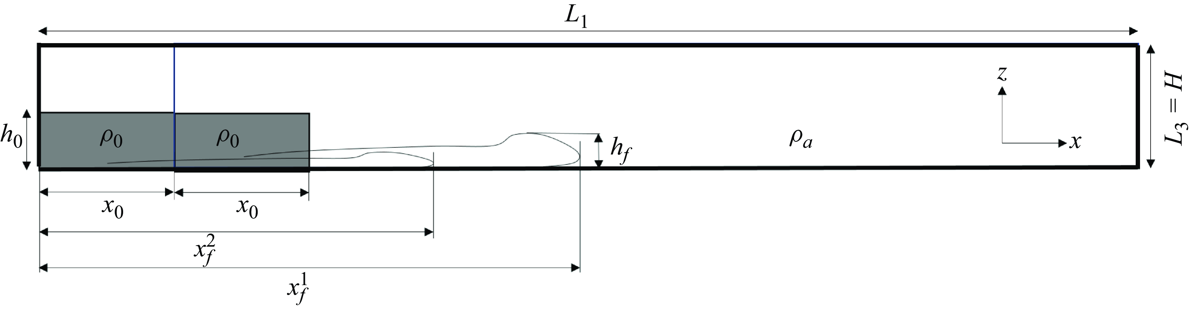


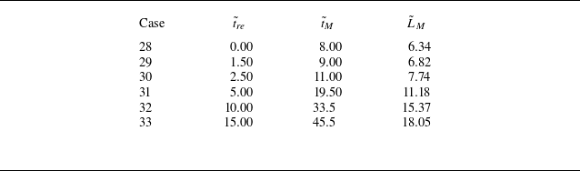


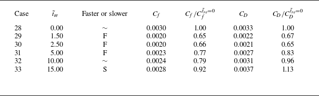


 Open access