


1. Introduction
Gravity currents induced by density differences in fluids are prevalent in various environmental and industrial flows. Under specific conditions, such currents can arise due to disparities in bulk density caused by suspended fine particles, commonly referred to as turbidity currents in geophysical contexts. Turbidity currents play a crucial role in sediment transport in the ocean, thereby significantly influencing the underwater environment (Milliman & Syvitski Reference Milliman and Syvitski1992; Meiburg & Kneller Reference Meiburg and Kneller2010). Consequently, numerous studies have been undertaken to investigate turbidity currents through laboratory experiments (Sequeiros, Mosquera & Pedocchi Reference Sequeiros, Mosquera and Pedocchi2018; Ouillon, Meiburg & Sutherland Reference Ouillon, Meiburg and Sutherland2019; Lippert & Woods Reference Lippert and Woods2020; Hitomi et al. Reference Hitomi, Nomura, Murai, De Cesare, Tasaka, Takeda, Park and Sakaguchi2021; Gadal et al. Reference Gadal, Mercier, Rastello and Lacaze2023), field observation (Warrick & Milliman Reference Warrick and Milliman2003; Dadson et al. Reference Dadson, Hovius, Pegg, Dade, Horng and Chen2005) and numerical simulations (Necker et al. Reference Necker, Hartel, Kleiser and Meiburg2002; Cantero, Balachandar & Garcia Reference Cantero, Balachandar and Garcia2008b; El-Gawad et al. Reference El-Gawad, Cantelli, Pirmez, Minisini, Sylvester and Imran2012; Chen, Geyer & Hsu Reference Chen, Geyer and Hsu2013; Nasr-Azadani & Meiburg Reference Nasr-Azadani and Meiburg2014; Espath et al. Reference Espath, Pinto, Laizet and Silvestrini2015; Tseng & Chou Reference Tseng and Chou2018). Studies in the numerical simulation category are typically conducted to examine large-scale dynamics using circulation models (El-Gawad et al. Reference El-Gawad, Cantelli, Pirmez, Minisini, Sylvester and Imran2012; Chen et al. Reference Chen, Geyer and Hsu2013; Tseng & Chou Reference Tseng and Chou2018) or to explore detailed flow physics using high-resolution computational fluid dynamics (CFD) solvers, such as direct numerical simulation (DNS) or large eddy simulation (Necker et al. Reference Necker, Hartel, Kleiser and Meiburg2002; Cantero et al. Reference Cantero, Balachandar and Garcia2008b; El-Gawad et al. Reference El-Gawad, Cantelli, Pirmez, Minisini, Sylvester and Imran2012; Nasr-Azadani & Meiburg Reference Nasr-Azadani and Meiburg2014; Espath et al. Reference Espath, Pinto, Laizet and Silvestrini2015). While it typically requires less parameterization for computing the fluid phase, the second methodology enables investigation into detailed physics. However, there exists a scale gap between field observations and what can be resolved by high-resolution CFD tools. The CFD studies usually aim to quantify specific dynamics in non-dimensional parameter spaces, allowing findings to be scaled up to more realistic scenarios. In the subsequent sections, we provide a survey of some important works in this category.
An early study by Necker et al. (Reference Necker, Hartel, Kleiser and Meiburg2002) was among the first to utilize a high-resolution flow solver to investigate turbidity currents in a lock-exchange configuration. By assuming inertialess particles in dilute suspension, the authors were able to model the transport of the particle concentration field using a single-phase scalar transport model. Incorporating this model with DNS enabled a detailed examination of flow structures, particle resuspension and deposition within turbidity currents. Necker et al. (Reference Necker, Hartel, Kleiser and Meiburg2002) also compared two-dimensional and three-dimensional simulation results, highlighting pronounced differences between the two strategies over a long time evolution. In a subsequent study employing a similar simulation strategy in a fully developed channel flow, Cantero et al. (Reference Cantero, Balachandar, Cantelli, Pirmez and Parker2008a) revealed intriguing results regarding self-stratification manifested through Reynolds-averaged sediment concentration, which led to turbulence suppression and flow relaminarization near the bottom. The authors proposed a criterion for identifying this flow regime based on an appropriately defined settling speed of particles. This issue of turbulence suppression was then further investigated in subsequent studies by the same group (Cantero et al. Reference Cantero, Balachandar, Cantelli, Pirmez and Parker2008a; Shringarpure, Cantero & Balachandar Reference Shringarpure, Cantero and Balachandar2012; Cantero, Shringarpure & Balachandar Reference Cantero, Shringarpure and Balachandar2012). Unlike the aforementioned studies modelling inertialess particles, Cantero et al. (Reference Cantero, Balachandar and Garcia2008b), drawing on scaling arguments from Ferry & Balachandar (Reference Ferry and Balachandar2001), introduced a more advanced transport model accounting for particle inertia due to drag. Their two-dimensional simulation results using this new model revealed changes in the spatial distribution of particles in the current due to particle–vortex interaction, including phenomena such as turbophoresis and preferential concentration. Moving beyond studies focusing on turbidity currents over flat channels, Nasr-Azadani & Meiburg (Reference Nasr-Azadani and Meiburg2014) conducted numerical investigations of currents interacting with the idealized bottom topography, i.e. a three-dimensional Gaussian bump. In addition to revealing changes in fine-scale flow structures induced by the bump, they found that the smaller bump resulted in faster current speeds by increasing the current's height, while the taller bump slowed the current down due to more rigorous three-dimensional motion. Another interesting feature of turbidity currents, or gravity currents more generally, is the lobe-and-cleft (LC) structure at the current's front, documented in numerous three-dimensional high-resolution numerical results, including those mentioned previously. Through highly resolved numerical simulations, Espath et al. (Reference Espath, Pinto, Laizet and Silvestrini2015) provided deposition maps in response to the LC structure and demonstrated that this pattern can also be found at deposited particles.
All the aforementioned numerical studies computed the transport of particle concentration by solving the scalar transport equation, rather than tracking the motion of individual particles. This approach allows for easy incorporation with the original DNS code and facilitates fast computation. However, there are drawbacks associated with this strategy. For example, while suspended particles with sizes ranging from  $d_0 \sim O$(1 $\mathrm {\mu }$m) to $O$(100 $\mathrm {\mu }$m) where $d_0$ is the particle diameter, molecular diffusion is infinitesimally small and negligible. Nevertheless, numerical diffusion or artificially added diffusivity in the numerical simulation is unavoidable. Another issue arises at the bottom where particles deposit. In fact, for the scalar transport model, deposition results in a slight change in domain height. Unless one employs a dynamic mesh technique, such as those implemented in Chou & Fringer (Reference Chou and Fringer2010) and Chou et al. (Reference Chou, Shao, Sheng and Cheng2019), accurate representation of the deposition of particle concentration becomes challenging. In this regard, these studies have utilized the penetration boundary condition, which allows the concentration flux of deposition to pass through the bottom boundary. However, this artificial boundary condition could lead to incorrect prediction of deposition, especially for large-sized, rapidly depositing particles. Consequently, most numerical studies have focused on suspension-dominated fine particles.
Recently, the successful integration of the discrete element model (DEM) and CFD, known as CFD-DEM (Kloss et al. Reference Kloss, Goniva, Hager, Amberger and Pirker2012; Blais et al. Reference Blais, Lassaigne, Goniva, Fradette and Betrand2016; Yang et al. Reference Yang, Low, Lee and Chiew2018), has enabled the simulation of turbidity currents by tracking the motion of individual particles. This advancement holds promise for producing results closer to real-world situations. In a recent study by Xie et al. (Reference Xie, Hu, Zhu, Yu and Pähtz2023), a CFD-DEM model incorporating LIGGGHTS and OpenFoam was utilized to investigate turbidity currents propagating down an inclined slope, with a specific focus on autosuspension. The study was able to discern the trajectory of autosuspended particles at the front of the current. Importantly, this approach circumvented the aforementioned issues associated with the scalar transport model and afforded a more comprehensive consideration of hydrodynamic forces acting on particles. The study uncovered significant characteristics of autosuspension at the current's front. However, due to the computationally intensive nature of tracking massive numbers of particles, the study was limited to lower Reynolds numbers (approximately 50), in contrast to previous studies employing scalar transport models. Consequently, for more rigorous flow regimes, such as those with Reynolds numbers typically of  $O(1000)$ in the aforementioned studies, a more detailed examination of particle–fluid interactions within turbidity currents remains necessary.
This study presents a series of numerical investigations of turbidity currents, with a particular focus on particle suspension and deposition. We are specifically interested in flow regimes akin to those observed in previous studies (i.e. Reynolds number  ${\sim } O(1000)$). To achieve a more precise modelling of particle motion, we employ a strategy similar to CFD-DEM. The fast particle tracking scheme (Chou, Gu & Shao Reference Chou, Gu and Shao2015) employed in our numerical model allows for the handling of a large number of particles within fine-resolution computational domains. Rather than focusing solely on the suspension-dominant regime for fine particles, our analyses delve into flow regimes where deposition plays a significant role. Through detailed numerical investigations utilizing particle tracking and DEM, this study aims to provide deeper insights into the dynamics of particle-laden turbidity currents across both suspension- and deposition-dominant regimes.
After introducing the methodology in § 2, the remainder of the paper is structured to achieve three primary goals. Firstly, we elucidate how flow structures of turbidity currents are influenced by varying particle sizes, thereby affecting particle suspension. This is discussed in § 3, followed by quantitative analyses for autosuspension in § 3.2. Secondly, we explore patterns of particle deposition in response to different flow features and particle sizes. This is detailed in § 4, where we elucidate the mechanisms leading to transverse and longitudinal variations in deposition height. Lastly, we propose a new scaling law to predict the bulk behaviour of the current, presented in § 5.
2. Methods
2.1. Governing equations for the particle phase
To describe particle motion, the momentum of a spherical particle with the diameter  $d_0$ and mass $m_p$ is described as
 \begin{align} m_p\dfrac{{\rm d}\boldsymbol{u}_p}{{\rm d}t} &= \alpha 3{\rm \pi} d_0 \mu (\boldsymbol{u}\vert_p-\boldsymbol{u}_p) + m_f\dfrac{1}{2}\left(\left.\dfrac{{\rm D}\boldsymbol{u}}{{\rm D}t}\right\vert_p - \dfrac{{\rm d}\boldsymbol{u}_p}{{\rm d}t}\right) -{\mathcal{V}}_p\boldsymbol{\nabla} P + (m_p-m_f)\boldsymbol{g}\nonumber\\ &\quad + 0.51J{\rm \pi} d_0^2 \sqrt{\dfrac{\mu \rho_f}{|\boldsymbol{\omega}|}} (\boldsymbol{u}\vert_p-\boldsymbol{u}_p)\times \boldsymbol{\omega} + \boldsymbol{F}, \end{align}
where  $\alpha$ is a coefficient to correct the drag accounting for finite Reynolds number and concentration, ${\rm d}/{\rm d}t$ is the material derivative of the particle moving with velocity $\boldsymbol {u}_p$, $\mu$ is the viscosity of the fluid phase, $\boldsymbol {u}$ is the velocity of the fluid phase, $m_f$ is the mass of the fluid, ${\mathcal {V}}_p$ is the volume of the particle, $P$ is the pressure, $\boldsymbol {g}$ is the gravitational acceleration, $J$ is a varying coefficient depending on the flow field, flow property and particle size, $\rho _f$ is the density of the fluid, $\boldsymbol {\omega }$ is the vorticity in the fluid phase, $\boldsymbol {F}$ is the collisional force and the notation $|_p$ indicates that the quantity is evaluated at the particle location $\boldsymbol {x}_p$. The terms in the right-hand side of (2.1) are (from left to right) drag, added mass, pressure, buoyant force, lift force and collisional force. In this study, we do not consider the Basset history force, which requires considerable computational effort but makes an insignificant difference in the numerical cases of the present study. This agrees with the previous studies by Xie et al. (Reference Xie, Hu, Zhu, Yu and Pähtz2023), who also suggested to neglect the history effect when modelling turbidity currents. For particle drag, we adopt the formulation proposed by Gidaspow (Reference Gidaspow1994), for which the correction coefficient $\alpha$ in (2.1) is written as
 \begin{equation} \alpha =\begin{cases} \dfrac{1}{1-\phi}\left[1 + 0.15\left(\dfrac{Re_p}{1-\phi}\right)^{0.687}\right] & \text{for}\ \dfrac{Re_p}{1-\phi} < 1000,\\ 0.44\dfrac{Re_p}{24} & \text{for}\ \dfrac{Re_p}{1-\phi} \ge 1000, \end{cases} \end{equation}
where
 \begin{equation} Re_p = \dfrac{\rho_f\vert(\boldsymbol{u}{\small |}_p - \boldsymbol{u}_p)\vert d_0}{\mu} \end{equation}
is the particle Reynolds number, and  $\phi$ is the volume fraction of particles. It should be noted that although the whole regime in (2.2) is considered in our numerical flow solver, only the first criterion is met in the present simulation cases. For particle lift, we consider the Saffman lift force (Saffman Reference Saffman1965), in which, following McLaughlin (Reference McLaughlin1991) and Mei (Reference Mei1992), the function $J$ is expressed as
 \begin{equation} J =0.3\left\{1+\tanh\left[\dfrac{5}{2}\left(\log_{10}\sqrt{\dfrac{\omega^*}{Re_p}}+0.191\right)\right]\right\} \left\{\dfrac{2}{3}+\tanh\left[6\sqrt{\dfrac{\omega^*}{Re_p}}\right]\right\}, \end{equation}
where  $\omega ^* = \vert \boldsymbol {\omega }\vert d_0/\vert (\boldsymbol {u}{\small \vert }_p - \boldsymbol {u}_p)\vert$.
Particle collision is a result of normal and tangential collisions. The collisional force on the particle  $k$ when it comes with particle $l$ is written as
 \begin{equation} \boldsymbol{F}_{kl} = \boldsymbol{F}_{n,kl} + \boldsymbol{F}_{t,kl}, \end{equation}
where the subscript  $n$ and $t$ indicate normal and tangential directions, respectively. In the present study, the soft-sphere collision model by Cundall & Strack (Reference Cundall and Strack1979) is used to model particle–particle and particle–wall collisions, which is expressed as
 \begin{equation} \boldsymbol{F}_{n,kl} =\begin{cases} -\gamma \delta_{kl,n}\boldsymbol{n}_{kl}-\xi \boldsymbol{u}_{kl,n} & \text{if}\ d_{kl} < r_k + r_l + \lambda,\\ 0 & \text{otherwise} , \end{cases} \end{equation}
where  $\gamma$ is a stiffness parameter, $\xi$ is the damping parameter, $d_{kl}$ is the distance between the centres of the particles, $\delta _{kl}$ is the overlap between particles, $\boldsymbol {n}_{kl}$ is the unit vector from the centre of particle $k$ to that of particle $l$,
$l$,  $\lambda$ is the force range, and $r_k$ and $r_l$ are the radii of particles $k$ and $l$, respectively. The relative normal velocity $\boldsymbol {u}_{kl}$ is given by
 \begin{equation} \boldsymbol{u}_{kl} = [(\boldsymbol{u}_{k}-\boldsymbol{u}_{l})\boldsymbol{\cdot} \boldsymbol{n}_{kl}]\boldsymbol{n}_{kl}. \end{equation}
Following Capecelatro & Desjardins (Reference Capecelatro and Desjardins2013), we employ a model for the damping parameter with the coefficient of restitution  $e$ (
$e$ ( $0< e<1$) and the effective mass $m_{p,kl} = (1/m_{p,k}+1/m_{p,l})^{-1}$, which is expressed as
 \begin{equation} \xi ={-}2 \ln e \dfrac{\sqrt{m_{p,kl}\gamma}}{\sqrt{{\rm \pi}^2+(\ln e)^2}}. \end{equation}
An expression of the stiffness parameter  $\gamma$ related to the collision time $\tau _{col}$ is given by
 \begin{equation} \gamma = \dfrac{m_{p,kl}}{\tau_{col}^2}({\rm \pi}^2 + \ln (e)^2). \end{equation}
In this study, we set  $e = 0.97$ following Chang et al. (Reference Chang, Huang, Chern and Chou2023) and $\tau _{col}$ as 15 times the computational time step to ensure the proper resolution of collision. For tangential collision, the collision force is described as
 \begin{equation} \boldsymbol{F}_{kl,t} = \min(|\boldsymbol{F}_{kl,t,LS}|, \mu_c |\boldsymbol{F}_{kl,n}|)\boldsymbol{e}_t, \end{equation}
where  $\mu _c$ is the friction coefficient, $\boldsymbol {e}_t$ is the unit vector of the tangential direction of the two colliding particles and
 \begin{equation} \boldsymbol{F}_{kl,t,LS} ={-}\gamma_t \delta_{kl,t}-\xi_t \boldsymbol{u}_{kl,t}. \end{equation}
Here, the friction coefficient  $\mu _c$ can represent either static friction $\mu _s$ or kinetic friction $\mu _k$ depending on the criteria proposed by Biegert, Vowinckel & Meiburg (Reference Biegert, Vowinckel and Meiburg2017).
2.2. Governing equations for the fluid phase
We focus on suspensions of spherical rigid particles in an incompressible fluid, for which conservation of momentum for the fluid phase can be described as
 \begin{equation} \dfrac{\partial}{\partial t} [(1-\phi)\boldsymbol{u}] + \boldsymbol{\nabla}\boldsymbol{\cdot}[(1-\phi)\boldsymbol{u}\boldsymbol{u}] ={-}(1-\phi)\boldsymbol{\nabla} P -\boldsymbol{f}_p + \boldsymbol{\nabla} \boldsymbol{\cdot} \boldsymbol{T}_{vis}, \end{equation}
where  $\phi$ is the volume fraction of the particle phase, $\boldsymbol {u}$ is the velocity of the fluid, $P$ is the dynamic pressure, $\boldsymbol {f}_p$ is the momentum feedback of the particle phase to the fluid phase and $\boldsymbol {T}_{vis}$ is the bulk viscous stress modelled as
 \begin{equation} \boldsymbol{T}_{vis} = (1-\phi)\nu [\boldsymbol{\nabla} \boldsymbol{u} + (\boldsymbol{\nabla} \boldsymbol{u})^{\textsf{T}}], \end{equation}
where  $\nu$ is the kinematic viscosity. Within the control volume (i.e. the grid cell), the momentum feedback is calculated by
 \begin{align} \boldsymbol{f\!}_p &= \sum_{j=1}^{N_c}s\phi_{p,j} \left[\dfrac{\alpha_j 3{\rm \pi} d_{0,j}\mu}{m_p} (\boldsymbol{u}\vert_{p,j}-\boldsymbol{u}_{p,j})+ \dfrac{1}{2s}\left(\left.\dfrac{{\rm D}\boldsymbol{u}}{{\rm D}t}\right\vert_{p,j} - \dfrac{{\rm d}\boldsymbol{u}_{p,j}}{{\rm d}t}\right)\right.\nonumber\\ &\quad +\left. \dfrac{0.51J_j{\rm \pi} d_{0,j}^2}{m_p} \sqrt{\dfrac{\mu\rho_f}{|\boldsymbol{\omega}|}}(\boldsymbol{u}\vert_{p,j}-\boldsymbol{u}_{p,j})\times \boldsymbol{\omega}\right], \end{align}
where  $j$ is the particle index, $s = m_p/m_f$ is the specific weight and $N_c$ is the number of particles within the control volume.
2.3. Link to the scalar transport model and scaling
Considering the gravity dominant cases (i.e.  ${\rm D}\boldsymbol {u}/{\rm D}t \sim {\rm d}\boldsymbol {u}_p/{\rm d}t \ll \boldsymbol {g}$) and small particles, (2.1) for a single particle (i.e. $\phi = 0$ and $\boldsymbol {F} = 0$) can be easily reduced to a drag-dominant equilibrium-state approximation
 \begin{align} \boldsymbol{u}_p &= \boldsymbol{u}\vert_p + \tau_p \boldsymbol{g}^\prime\nonumber\\ &=\boldsymbol{u}\vert_p - w_s \boldsymbol{e}_3, \end{align}
where
 \begin{equation} \tau_p = \dfrac{sd_0^2}{18\nu} \end{equation}
is the particle relaxation time,  $\boldsymbol {g}^\prime = (1-1/s)\boldsymbol {g}$ is the reduced gravitational acceleration, $w_s = \tau _p g^\prime$ is the settling velocity of the particle and $\boldsymbol {e}_3$ is the unit direction vector in the $z$-direction, which is defined as the direction of the gravitational force. To reach (2.15), we have also assumed $\alpha = 1$ (i.e. $Re_p \ll 1$) and we drop the term whose order of magnitude is lower than $O(d_0)$ for those involving the velocity difference between the two phases.
Substituting the first identity of (2.15) for a number of particles resulting in a volume concentration  $\phi$ into (2.12) and assuming that $\phi \ll 1$ for the case of dilute suspension, under the Boussinesq approximation, the momentum equation for the fluid phase can be rewritten as
 \begin{equation} \dfrac{\partial \boldsymbol{u}}{\partial t} + \boldsymbol{\nabla}\boldsymbol{\cdot}(\boldsymbol{u}\boldsymbol{u}) ={-}\boldsymbol{\nabla} P +\phi \boldsymbol{g}^\prime + \nu \nabla^2 \boldsymbol{u}. \end{equation}
Moreover, according to the second identity of (2.15), along with the particle diffusion, transport of particle concentration  $\phi$ can be modelled with
 \begin{equation} \dfrac{\partial \phi}{\partial t} + \boldsymbol{\nabla}\boldsymbol{\cdot}(\boldsymbol{u}\phi) + w_s\dfrac{\partial \phi}{\partial z} = \kappa_s \nabla^2 \phi, \end{equation}
where  $\kappa _s$ is the particle diffusivity arising from particle–particle and particle–hydrodynamics interactions (e.g. Davis Reference Davis1996; Segre et al. Reference Segre, Liu, Umbanhowar and Weitz2001). Equations (2.17) and (2.18) are the simplified governing equations frequently used for modelling sediment transport in both laboratory- and field-scale cases. As an in-depth discussion on different modelling strategies is beyond the scope of the present study, readers may refer to Shao, Hung & Chou (Reference Shao, Hung and Chou2017) for more detailed explanations about the relationship between the Euler–Lagrange formulation and the traditional scalar transport model. Additionally, readers can refer to earlier studies by Ferry & Balachandar (Reference Ferry and Balachandar2001), Cantero et al. (Reference Cantero, Balachandar and Garcia2008b) or Chou, Wu & Shih (Reference Chou, Wu and Shih2010) on non-Equilibrium sediment transport modelling for a more detailed derivation on the connections between different modelling stratifies for sediment transport.
In this approximation, the momentum feedback of particles to the bulk flow becomes a buoyant force  $\phi \boldsymbol {g}^\prime$. Therefore, using the initial height of the particle slump $L_{0,z}$ as the characteristic length scale and initial particle concentration $\phi _0$, one may define a buoyancy velocity scale
 \begin{equation} U = \sqrt{\tfrac{1}{2}L_{0,z}\phi_0 g^\prime}, \end{equation}
where  $g^\prime = |\boldsymbol {g}^\prime |$. A time scale of the bulk flow can be thus defined as
 \begin{equation} T_f = \dfrac{L_{0,z}}{U}. \end{equation}
For a single particle, the buoyancy force per mass is  $\boldsymbol {g}^\prime$, such that one may define a buoyancy time scale for individual particles as
 \begin{equation} T_b = \dfrac{U}{g^\prime}. \end{equation}
Using (2.19) and (2.20) as scaling parameters and dropping the particle collision term for the dilute suspension regime, rearrangement of (2.1) yields
 \begin{align} \dfrac{\phi_0}{2}\dfrac{{\rm d}^*\boldsymbol{u}_p^*}{{\rm d}^*t^*} &= \alpha \dfrac{\boldsymbol{u}^*\vert_p-\boldsymbol{u}^*_p}{St} + \dfrac{\phi_0}{4s}\left.\Bigg(\dfrac{{\rm D}^*\boldsymbol{u}^*}{{\rm D}^*t^*}\right\vert_p - \dfrac{{\rm d}^*\boldsymbol{u}_p}{{\rm d}^*t^*}\Bigg) -\dfrac{\phi_0}{2s}\nabla^* P^* - \boldsymbol{e}_3\nonumber\\ &\quad +C_LT_b(\boldsymbol{u}^*\vert_p-\boldsymbol{u}^*_p)\times \dfrac{\boldsymbol{\omega}}{|\boldsymbol{\omega}|}, \end{align}
where the superscript  $*$ denotes the dimensionless quantities, $C_L = 3.06J\sqrt {\nu |\boldsymbol {\omega }|}(s d_0)^{-1}$ is the lift coefficient, and
 \begin{equation} St = \dfrac{\tau_p}{T_b} \end{equation}
is the Stokes number, which is also equivalent to the dimensionless settling speed,  $w_s^* = w_s/U$. Equation (2.22) shows that in the dilute suspension regime where $\phi _0 \ll 1$ and ${\alpha \sim 1}$, all the transient terms become negligible, and only the lift force causes the deviation of the particle from its drag state (2.15). From (2.22) and the definition of $C_L$, the ratio between the drag and lift can be found as
 \begin{equation} \dfrac{\text{drag}}{\text{lift}} = 5.88\dfrac{s}{Jd_0}\sqrt{\dfrac{\nu}{|\boldsymbol{\omega}|}}. \end{equation}
To obtain an estimation of the magnitude in (2.24) for suspension in water in this study, substitution of a reference value  $J = 2.255$ (McLaughlin Reference McLaughlin1991), the specific weight $s = 2.65$, the maximum particle size $d_0 = 99$ $\mathrm {\mu }$m and $|\boldsymbol {\omega }| = 30$ s $^{-1}$, which is approximately the maximum value of the vorticity in the present simulation cases, (2.24) gives a magnitude of $O(10)$ for the ratio between the drag and lift. This scaling analysis shows that even though more complete hydrodynamic interactions between the particle and fluid phases are considered in the present study, only the drag and buoyancy force dominate particle motion, making (2.15) valid in the suspension regime.
2.4. Numerical methods
Calculations of particle momentum and movement are implemented in an incompressible flow solver originally developed by Zang, Street & Koseff (Reference Zang, Street and Koseff1994) and then parallelized by Cui (Reference Cui1999). In this code, the governing equations are discretized using a finite-volume method on non-staggered grids. All spatial derivatives except the convective terms are discretized with second-order central differences. The convective terms are discretized using a variation of QUICK (Leonard Reference Leonard1979; Perng & Street Reference Perng and Street1989). The second-order Crank–Nicolson scheme is used for the time advancement of the diagonal viscous terms, and the second-order Adams–Bashforth method is used for all others. For the particle phase, the third-order Runge–Kutta method is used for the time advancement of particle motion. The original flow solver has been successfully applied to simulations of numerous flow problems (e.g. Zang et al. Reference Zang, Street and Koseff1994; Zang & Street Reference Zang and Street1995; Cui & Street Reference Cui and Street2001; Fringer & Street Reference Fringer and Street2003; Chou & Fringer Reference Chou and Fringer2008). More recently, the version along with a fast point-particle tracking method was developed by Chou et al. (Reference Chou, Gu and Shao2015), which was then applied to study convective sedimentation (Chou & Shao Reference Chou and Shao2016; Shao et al. Reference Shao, Hung and Chou2017), particle segregation (Lai, Lin & Chou Reference Lai, Lin and Chou2023) and direct energy deposition (Chou, Mai & Tseng Reference Chou, Mai and Tseng2021). In this flow solver, the added mass effect and pressure coupling between the particle and fluid phases are treated implicitly. Details of the implementation for the calculation of particles can be found in Chou et al. (Reference Chou, Gu and Shao2015).
2.5. Simulation set-up
Simulations were conducted by releasing a fixed-sized particle-laden fluid column in a three-dimensional rectangular domain, as schematically shown in figure 1. In this study, we use the initial height of the particle-laden fluid column,  $L_{0,z} = 0.05$ m, to normalize all the spatial dimensions. With the gravitational force acting in the $z$-direction, the size of the initial size of the particle-laden fluid column is given by $L_{0,x} \times L_{0, y} \times L_{0, z} = 0.4 \times 2 \times 1$, and the simulation domain is given by $L_x \times L_y \times L_z = 6 \times 2 \times 1.5$ with a grid resolution of $1152 \times 384 \times 288$. The periodic boundary condition was applied to the boundaries in the $y$-direction. The no-slip boundary condition was applied to the boundaries at the bottom and two ends in the $x$-direction, while the free-slip was applied to the top boundary. We used three different initial particle concentrations, $\phi _0 = 0.005$, $0.01$ and $0.02$ (in volume fraction), with six different particle diameters $d_0 = 53$, $65$,
$65$,  $75$,
$75$,  $84$,
$84$,  $99$,
$99$,  $112$
$112$  $\mathrm {\mu }$m. The initial particle concentrations result in the Grashof number,
 \begin{equation} Gr = \left(\dfrac{UL_{0,z}/2}{\nu}\right)^2, \end{equation}
ranging from  $1 \times 10^6$ to $5 \times 10^6$ and the Reynolds number,
 \begin{equation} Re = \dfrac{UL_{0,z}}{2\nu}, \end{equation}
ranging from 1000 to 2000. Given by the present particle sizes and initial concentrations, the buoyancy Stokes number (referred to as the Stokes number here after) ranges from  $O(0.01)$ to $O(0.1)$. As each simulation case involves the computational handling of a massive number of particles, the number of particles was based on our limited computational resources, while its concentrations and initial current height are set to match the values of the Grashof number in the previous study by Necker et al. (Reference Necker, Hartel, Kleiser and Meiburg2002) using the scalar transport model. Initially, particles were randomly distributed in the particle-laden region, resulting in a concentration equivalent to the desired bulk concentration. Each case was initialized with a fixed white-noise perturbation to each momentum component with a mean velocity amplitude of $0.08$. Moreover, to trigger turbulence, a multimode perturbation is applied to the particle-laden interface in the $x$-direction (i.e. at $x = 0.4$) with the wavelength ranging from 0.04 to 1 and mean displacement of 0.01.
Schematic showing the domain configuration of the present simulation. The grey shaded area represents the initial particle-laden region.

As presented in Appendix A, a grid convergence test using the single-phase approach was conducted to ensure that the convergence of the simulation result can be reached at the current grid resolution given by the desired buoyancy condition. In what follows, we adopt the convention in which cases are named with a combination of three significant digits after the decimal point of the particle concentration following the letter ‘V’ and two significant digits after the decimal point of  $St$ following the letters ‘St’. For example, the case with the particle volume fraction $\phi _0 = 0.01$ and $St = 0.10$ ( $d_0 = 84$ $\mathrm {\mu }$m) is named case V010St10. For comparison, we also conducted two single-phase simulation cases with $\phi _0 = 0.01$. In the first case, named V010SP, we solve the scalar transport with an equivalent buoyant effect without a gravity-induced settling. The second single-phase case, V010SPSt04, is similar to V010SP except that a settling speed ( $w_s$) was added to the transport equation (2.18). The added $w_s$ is the same as the settling speed at the equilibrium state (i.e. (2.15)) in case V010St04. This case was conducted to compare the present particle-tracking model with the traditional single-phase model. In both single-phase cases, we employed a diffusivity $\kappa _s = 10^{-7}$ m $^{2}$ s $^{-1}$, which is slightly higher than the numerical diffusivity of our solver. Details for all of the present simulation cases are summarized in table 1. The present simulation cases were conducted using the Intel Platinum 8280L 28 Cores 2.7 GHz central processing unit (CPU) at the National Center for High-performance Computing (NCHC). The Eulerian–Lagrangian calculations, such as case V010St04, were conducted using 192 cores, which took approximately 54 h for 30 000 computational steps. Required CPU time increases when the number of particles increase. The single phase calculation, such as case V010SP, took approximately 19 h for 30 000 computational steps using the same computational resources. In the rest of this paper, in addition to the aforementioned $L_{0,z}$ and $U$ as the characteristic length and velocity, respectively, $T = L_{0,z}/U$ and $\phi _0$ are characteristic time and concentration for the non-dimensionalization of the respective physical quantities. In what follows, dimensional quantities are denoted with the superscript $*$.
$*$.
Simulation set-up of the present cases. The superscript  $*$ indicates the dimensional quantity.

The validity of the point-force representation in the present simulation cases can be justified by comparing the particle size with the smallest flow scale, the Kolmogorov scale, which is expressed in non-dimensional form as
 \begin{equation} l_0 = \left(\dfrac{1}{Re^3\epsilon}\right)^{0.25}, \end{equation}
where
 \begin{equation} \epsilon = \dfrac{1}{Re}\dfrac{\partial u_i^\prime}{\partial x_k}\dfrac{\partial u_i^\prime}{\partial x_k} \end{equation}
is the turbulent energy dissipation. To obtain the turbulent fluctuation quantity  $u_i^\prime$, an ensemble mean of each velocity component $\langle u_i\rangle$ is required. Here, $\langle u_i\rangle$ is approximated by a spanwise average of the instantaneous velocity field $\langle u_i\rangle _{span}$, and the fluctuation quantity is thus calculated by
 \begin{equation} u_i^\prime = u_i-\langle u_i\rangle_{span}. \end{equation}
Figure 2 shows the estimated dissipation rate at a representative time step during the full development of the current in case V020St03, which has the strongest buoyant forcing. The highest value is approximately 0.03 in this figure, leading to  $l_0 \sim 0.007$ according to (2.27), which is larger than the largest dimensionless particle size, $d_0 = 0.002$, and dimensionless grid resolution ( $= 0.005$) in this study. Therefore, it can be concluded that the point-force representation is a valid approximation for the flow configuration of the present study.
The estimated turbulent energy dissipation ( $\epsilon$) at $t = 3.9$ in case V020St03.

Figure 3 presents a comparison between the present simulation results in cases with  $\phi _0^*$ and experimental data from Gladstone et al. (Reference Gladstone, Phillips and Sparks1998), showing the dimensionless time histories of the front travel distance, $x_f$. The simulation results indicate that $x_f$ initially increases with time almost at a constant slope, followed by a smooth transition to the end of the motion. It can be seen that before the transition, there is good agreement between the present simulation results and experimental data. As discussed in the following section, the cessation of the propagation is due to the increasing importance of particle settling. Therefore, the propagation ends earlier with increasing particle size (i.e. large $St$). Figure 3 shows that our simulation results agree with experimental data before the transition to the cessation. Moreover, as $St = 0.01$ was used in the experiment of Gladstone et al. (Reference Gladstone, Phillips and Sparks1998), the transition occurs later in time compared with our simulation cases, which is consistent with our simulation results.
Comparison of the travel distance of the front,  $x_f$, as a function of time between the present simulation results in cases of $\phi _0^* = 0.01$ with different $St$ and the experimental data from Gladstone, Phillips & Sparks (Reference Gladstone, Phillips and Sparks1998).

3. Suspension
3.1. Flow evolution
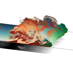
Figure 4 presents the time histories of the front speed  $U_f$, in cases V010St04, V010SPSt04 and V010SP, along with three-dimensional snapshots of particles in the former case at representative time instants during the evolution of the current. In figure 4(b–e), particles released from different initial regions are located by marking with different colours, revealing the patterns of mass transport within the current. The front speed is obtained by averaging the speed at the most frontal points in the current along the $y$-direction. Figure 4(a) shows that the current first undergoes a fast acceleration stage due to the initial release of potential energy. A representative snapshot of the current is shown in figure 4(b). After reaching a peak value, the front speed decreases rapidly, forming the second stage, as indicated by the interval between the first two triangles in the case V010St04 in figure 4(a). This second stage is marked by the rapid drop of the current's height, which can be observed by the locations of the pink-coloured layer in figure 4(b,c). The front velocity decreases due to decreasing current height until the pink layer ceases falling, after which the third stage begins. The first two stages make up the initial slumping stage, at the end of which is the onset of the horizontal current, as shown in figure 4(c). It can be seen from figure 4(a) that front speeds in particle-laden and scalar cases are fairly close to each other in the initial slumping stage, indicating the dominance of the buoyancy effect during this stage. It should be noted that the initial slumping stage referred to here differs from the ‘slumping’ described in the early study by Rottman & Simpson (Reference Rottman and Simpson1983), which was used to define the entire process of the density current. including the subsequent stage of horizontal propagation.
Time histories of the front speed in cases V010St04, V010SPSt04 and V010SP (a), along with three-dimensional snapshots of particles at  $t = 0.6$ (b), $1.4$ (c), $2.9$ (d) and $4.1$ (e), which are representative time instants marked by triangles in (a). In (b–e), particles released from different initial regions are located by marking with different colours.

In the third stage, the current moves horizontally, but at the same time, particles settle onto the bed, causing the evolution of the front speed to drop more rapidly than in the scalar case. A snapshot of particles in this stage is shown in figure 4(d). This stage, termed the propagation stage hereafter, is characterized by the settling of particles and the induced buoyancy effect being equally important. While the latter drives the current to propagate horizontally, the former slows down the current through the reduction of the buoyancy force. Also, the roll-up at the front becomes significant, as shown in figure 4(c,d), a large portion of the particles initially located at the bottom are suspended into the fluid column. After a relatively slow deceleration, the front speed drops abruptly at  $t \sim 4$. This is the time when a large portion of particles have settled onto the bed, as shown in figure 4(e), while those remaining in the water column continue to drive the slow motion of the current. Due to the diminished buoyancy effect, this stage is primarily characterized by dissipation resulting from particle settling, and is henceforth referred to as the dissipation stage. In contrast to the scalar case, where the deceleration of the front speed is primarily due to mixing between the current and ambient fluid, in the particle case, the deceleration of the front speed is more pronounced, primarily attributed to gravitational settling of particles.
A comparison between cases V010St04 and V010SPSt04 reveals that the front velocities in these two cases are very close during the early stages (i.e.  $t < 5$), with the latter case showing lightly lower values. This similarity between them is due to the small $St$ and the dilute particle concentration ( $\phi ^* \sim 0.01$) in the present cases. However, the results from the two cases begin to deviate significantly from each other in the later stage when $t > 5$. The disparities can be attributed to two reasons. First, as demonstrated by the energy budget analysis in § 3.2, the equilibrium-state approximation (2.15) adopted by the single-phase model in case V010SPSt04 can result in slightly faster settling of particles than that in the present inertia particle cases. The difference caused by this small difference in particle settling can become significant in the later stage when a major portion of particles have settled onto the bed. The second reason is the diffusive nature of the scalar transport in the single phase model. Since particles in our study do not diffuse (i.e. particles of the current sizes in nature typically have negligible molecular diffusivity), the difference between scalar transport and particle tracking can become significant when the concentration becomes extremely dilute in the later stage.
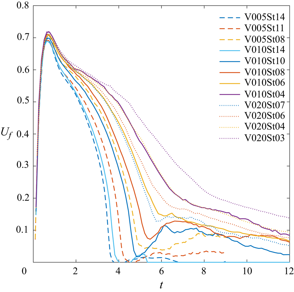
Figure 5 compares the time history of the front speed for all particle cases considered in this study. It is evident that during the initial slumping stage, for cases with  $St < 0.1$, front speeds show little variation across different particle sizes, indicating the predominant influence of buoyancy, particularly for small particles. The maximum front speed observed in these cases is 0.72. However, in cases with $St > 0.1$, a slight decrease in front speed is observed with increasing $St$, attributed to the rapid settling of particles which hinders the development of the buoyancy effect. This suggests that for large particles ( $St \ge 0.1$), particle settling outpaces the development of the buoyancy effect. Conversely, in conditions where $St < 0.1$, such as those simulated in this study, gravitational settling of particles is negligible in the initial slumping stage, with the dominant force being buoyancy. Moving to the propagation stage, figure 5 illustrates notable differences among cases with varying particle sizes. Particularly, it is observed that as the particle size increases, the front speed drops more rapidly, highlighting the significant impact of particle size during the propagation stage.
Time histories of the front speed in all of the present cases.
3.2. Autosuspension and energy budget
Figure 6 compares results from cases with two different particle sizes (cases V010St04 and V010St10), presenting particles coloured by their vertical velocity and superimposed with flow velocity vectors at the central slide in the  $y$-direction. In this figure, particles exhibiting autosuspension are identified by observing the colours indicating the particle's vertical velocity. The autosuspension at the front region plays a crucial role in sustaining the propagation of the current (Bagnold Reference Bagnold1962). Here, particles instantaneously moving upward are defined as autosuspended particles, following the classification in a recent study by Xie et al. (Reference Xie, Hu, Zhu, Yu and Pähtz2023). Unlike the low- $Re$ cases in Xie et al. (Reference Xie, Hu, Zhu, Yu and Pähtz2023), where autosuspension regions are primarily observed only at the current's head, a significant portion of autosuspension is also found at the current's body due to Kelvin–Helmholtz instability in the smaller-particle case, clearly depicted in figure 6(e, f). Additionally, figure 6 reveals that the number of autosuspended particles increases with decreasing particle size.
Particles coloured by their vertical velocity and superimposed with flow velocity vectors at the central slide in the  $y$-direction in cases V010St10 (a–c) and V010St04 (d–f) at $t = 1.4$ (a,d), $3.1$ (b,e) and $3.7$ (c, f).

For Lagrangian particles, we analyse the total energy budget following the formulation in Chou & Shao (Reference Chou and Shao2016), with modification of particle dissipation. That is, the release of potential energy due to the movement of particles ( $\Delta {PE}_p$) is the sum of the kinetic energy of the carrier fluid ( ${KE}_c$), kinetic energy of particles ( ${KE}_p$), viscous dissipation ( $\varTheta$) and particle dissipation ( ${PD}$), i.e.
 \begin{equation} \Delta {PE}_p (t) = {KE}_c (t) + {KE}_p (t) + \varTheta (t) + {PD} (t), \end{equation}
where
 $$\begin{gather} \Delta {PE}_p(t) = 2\int_{t^\prime = 0}^{t} {\mathcal{V}}_p \sum_{j = 1}^{N_{tot}}\boldsymbol{u}_{p,j} \boldsymbol{\cdot} \hat{\boldsymbol{e}}_z \,{\rm d}t^\prime, \end{gather}$$
 $$\begin{gather}{KE}_p(t) = s{\mathcal{V}}_p\sum_{j = 1}^{N_{tot}} \dfrac{1}{2}|\boldsymbol{u}_{p,j}|^2, \end{gather}$$
 $$\begin{gather}{KE}_c(t) = \int_{\varOmega} \dfrac{1}{2}(1-\phi^*)|\boldsymbol{u}|^2 \,{\rm d}\mathbb{V}, \end{gather}$$
 $$\begin{gather}\varTheta(t) = \dfrac{1}{Re}\int_{t^\prime = 0}^{t}\int_\varOmega \boldsymbol{u} \boldsymbol{\cdot} (\boldsymbol{\nabla} \boldsymbol{\cdot} \boldsymbol{T})\,{\rm d}\mathbb{V}\,{\rm d}t^\prime \end{gather}$$
and
 \begin{equation} {PD}(t) = \int_{t^\prime = 0}^{t} s{\mathcal{V}}_p \left(\sum_{j = 1}^{N_{tot}} \dfrac{\vert \boldsymbol{u}_{p,j}-\boldsymbol{u}\vert_{p,j}\vert}{St} + \sum_{j = 1}^{N_{tot}}\boldsymbol{u}_{j,k}\boldsymbol{\cdot} \boldsymbol{C}_{j} + \sum_{j = 1}^{N_{tot}}\boldsymbol{u}_{p,j}\boldsymbol{\cdot} \boldsymbol{F}_{j}\right) {\rm d}t^\prime, \end{equation}
where  ${\rm d}\mathbb {V} = {\rm d}\kern0.7pt x\,{\rm d}y\,{\rm d}z$ stands for the infinitesimal volume element of the computational domain $\varOmega$. Equation (3.6) accounts for energy dissipation due to hydrodynamic interactions and particle–particle collisions (see § 2), where $\boldsymbol {C}_{k}$ stands for all the hydrodynamic forcing terms in the right-hand side of (2.22) except the drag. In (3.6), the third term in the integral is important only in the deposition region where the particle concentration is high, which occupies a very small portion of the domain. One may divide the total number of particles ( $N_{tot}$) into suspension and deposition regimes, i.e.
 \begin{equation} N_{tot} = N_{sus} + N_{dep}, \end{equation}
where  $N_{sus}$ and $N_{dep}$ represent the total number of particles in suspension and deposition, respectively. Now, we define a equilibrium particle dissipation as
 \begin{equation} {PD}_{eq}(t) = \int_{t^\prime = 0}^{t} s{\mathcal{V}}_p \left(N_{sus} + \sum_{j = 1}^{N_{dep}}\boldsymbol{u}_{p,j}\boldsymbol{\cdot} \boldsymbol{F}_{col, j}\right) {\rm d}t^\prime, \end{equation}
which is formulated based on the assumption that for each individual particle in suspension, the hydrodynamic drag is in balance with the gravitational force, such that  $\boldsymbol {u}_{p,k} = \boldsymbol {u}\vert _{p,k}-w_s\hat {\boldsymbol {e}}_3 = \boldsymbol {u}\vert _{p,k}-St\,\hat {\boldsymbol {e}}_3$. Because particles in deposition normally have very low velocity, to obtain $N_{sus}$ and $N_{dep}$ in (3.8), particles with $|\boldsymbol {u}_{p,k}| < w_s$ are treated as deposited particles, while those with $|\boldsymbol {u}_{p,k}| \ge w_s$ are considered suspended particles.
Figure 7 presents the temporal evolution of the normalized energy budget in representative cases, including one employing the scalar transport model. All quantities in this figure are normalized by the initial available potential energy, denoted by a tilde. In this figure, except for the scalar case shown in figure 7(c), each row represents cases with the same initial concentration but increasing particle size (i.e. increasing  $St$). In each case, the accumulated release of potential energy of autoresuspended particles is also plotted.
Temporal evolution of energy budget in cases (a) V020St03, (b) V020St06, (c) V010SP, (d) V010St04, (e) V010St10, ( f) V010St14, (g) V005St06, (h) V005St11 and (i) V005St14. In (a), the two dashed lines highlight the flattened region of  $\Delta \widetilde {{PE}}_p$ following the initial sudden rise, and the arrow indicates a value of $\widetilde {{PD}}$ that is much higher than $\widetilde {{PD}}_{eq}$.

Generally, the potential energy release ( $\Delta \widetilde {{PE}}_p$) undergoes a sudden rise in the initial slumping stage, leading to a corresponding increase in the flow's kinetic energy. The kinetic energy of particles is negligible in all particle cases due to their small volume fractions. In contrast to the particle cases, where $\Delta \widetilde {{PE}}_p$s soon reach their maximum capacities ( $\Delta \widetilde {{PE}}_p \sim 1$) with smooth transitions, the scalar case (see figure 7c) exhibits a slight drop followed by a slow increase in $\Delta \widetilde {{PE}}_p$ at an almost constant rate. In the scalar case, viscous dissipation is the primary mechanism for flow dissipation, while in the particle cases, particle dissipation becomes equally important in dissipating flow energy. The combination of particle dissipation and viscous dissipation significantly accelerates the release of potential energy.
In cases involving fine particles (such as in figure 7a,d), a relatively flat region is present in the time history of  $\Delta \widetilde {{PE}}_p$ following the initial sudden rise, as highlighted by the region between two dashed lines in figure 7(a). This indicates a delay of particle settling, which sustains the horizontal motion of the current. The significance of this flattened zone decreases with increasing particle size and is almost absent in the largest-particle cases (e.g. figure 7f,i), indicating the dominance of initial slumping without significant horizontal propagation. Furthermore, figure 7(a,d) demonstrate that this flattened zone is accompanied by an increase in negative potential energy release of autosuspended particles, $\Delta \widetilde {{PE}}_{auto}$. Note that a negative value of potential energy release indicates particle suspension. The flattened zone ceases when $\Delta \widetilde {{PE}}_{auto}$ reaches its negative peak, suggesting that autosuspension drives the horizontal propagation of turbidity currents. In cases involving large particles where $St > 0.1$, significantly fewer particles can be autosuspended due to the limited range of the vertical velocity at the front region. Consequently, the change in potential energy release due to autosuspension becomes negligible, as shown in figure 7(c, f,h,i).
A crucial observation in figure 7 highlights the disparity between the actual particle dissipation ( $\widetilde {{PD}}$) and the equilibrium model ( $\widetilde {{PD}}_{eq}$), which neglects particle inertia. Notably, the latter, combined with the scalar transport model, have been extensively utilized in the sediment transport community (see § 2.1). Figure 7 illustrates that during the initial slumping stage (i.e. $t < 1$), neglecting particle inertia can lead to an underestimation of particle dissipation. This underestimation becomes particularly pronounced for smaller $St$. For instance, in the case with the smallest $St$ ( $= 0.03$), the underestimation nearly reaches $50\,\%$ of its original magnitude, as indicated by the arrow in figure 7(a). Conversely, in those cases with $St > 0.1$, this underestimation is negligible, and the equilibrium assumption closely aligns with actual particle dissipation (figure 7f,h,i). This suggests that particle inertia enhances settling during the initial slumping stage, during which vertical motion dominates. The enhancement is more significant for cases with smaller $St$.
$St$.
When the horizontal motion becomes dominant following the conclusion of the initial slumping stage, the equilibrium assumption starts to slightly overestimate the particle dissipation. This implies that when horizontal motion dominates, assuming the particle drag balances the gravitational force, can lead to an overestimate of particle dissipation (i.e. faster settling). This overestimation becomes more pronounced with increasing  $St$. In the case of the largest $St$, the overestimate reaches approximately $10\,\%$ of the actual particle dissipation (figure 7f). Conversely, for the smallest $St$,
$St$,  $\widetilde {{PD}}_{eq}$ closely matches $\widetilde {{PD}}$, suggesting that the equilibrium assumption can be a suitable approximation for small particles (e.g. $St \ll 1$) in predicting horizontal current propagation.
4. Deposition
4.1. Deposition in response to LC structure
The formation of LC features at the interface of a density current front is a well-known phenomenon. In this section, our objective is to elucidate particle deposition within the current in response to the LC structure. Taking case V010St04 as an illustration, figure 8 showcases the isosurface of bulk particle concentration ( $\phi$), the corresponding velocity field in the bottom-most horizontal plane, and the velocity field superimposed with particles at a representative cross-section at the front. This figure serves as a typical example of how particles respond to the LC instability at the current's front region. In figure 8(b), the $z$-component vorticity field ( $\omega _3$) is overlaid with velocity arrows to aid in distinguishing between the converging and diverging horizontal flow. In this figure, particle zones that show neither blue nor red colours indicate divergent flow, while those with adjacent blue and red colours represent converging flow. It is evident in figure 8(b) that the lobe structure corresponds to a divergence of the horizontal flow, while the cleft corresponds to convergence. Due to mass conservation, convergence of the horizontal flow at the cleft leads to an upward flow, suspending particles, while particles in the lobe region continue to settle. This is illustrated in figure 8(c), where we present snapshots of the flow field superimposed with particles on three consecutive vertical slices ( $z$–
$z$– $y$ plane) in the front region indicated in figure 8(a). This dynamic process results in the formation of an LC pattern in the deposition height, where lobes are separated by ditches formed by particle suspension at the cleft region. This phenomenon is demonstrated in figure 9, where we present the height of particle deposition ( $h_d$) within the current at representative time steps in case V010St04. Here, the height is calculated by summing the equivalent height in each cell where the particle concentration reaches close packing, i.e.
 \begin{equation} h_d(x, y) = \dfrac{1}{1-n^*}\left(\sum_{k=1}^{N_{cp}}\phi_k^* + \phi_{N_{cp}+1}^*\right)\Delta z, \end{equation}
where  $k$ is the cell index in the $z$-direction, $n^*$ is the void ratio and $N_{cp}$ is the cell index of the grid cell within which particles are close packed (i.e. $\phi ^* \ge 1-n^*$) (i.e. close packed). According to Scott & Kilgour (Reference Scott and Kilgour1969), the void ratio for the close-packed particles ranges from 0.3 to 0.5. Here, we simply set $n^*$ to 0.4. The second term on the right-hand side of (4.1) represents the particle concentration in the cell, which is partially occupied by the close-packed particles, on top of the grid cell with index $N_{cp}$.
(a) The isosurface of the bulk particle concentration ( $\phi = 1$) at $t = 2.7$ in case V010St04, (b) the corresponding horizontal velocity arrows at the bottom-most plane ( $x$–
$x$– $y$ plane at $z = 2.6 \times 10^{-3}$ superimposed with the vorticity ( $\omega _3$) and particles and (c) the vertical velocity superimposed with particles and velocity arrows on the vertical slices ( $z$–
$z$– $y$ plane) in the front region shown in (a).

The deposition height ( $h_d$) at $t = 1.3$ (a), 2.5 (b), 3.8 (c), 5.1 (d), 6.4 (e) and 8.9 ( f) in case V010St04. The red arrows in (d–f) indicate the positions of the vertical slices depicted in figure 10.


As shown in figure 9(a), fine LC structures of deposition are present at the very early stage. Subsequent to this, figure 9(b,c) demonstrate the gradual coarsening of the LC deposition pattern due to the amalgamation of fine LC structures. Notably, the deposition pattern in  $h_d$ is primarily observed in close proximity to the front region, where significant upward flow prevails. Behind the front region, the LC pattern vanishes due to the continuous deposition of suspended particles. As the current progresses into its dissipation stage, its velocity decreases notably owing to the diminished driving buoyancy force. During this phase, smaller lobes tend to merge while larger ones remain relatively unchanged, as shown in figure 9(d,e).
Figure 10 illustrates particles superimposed with the velocity field in representative vertical slices ( $z$–
$z$– $y$ plane) in the front regions corresponding to the cases depicted in figure 9(d–f). In contrast to the flow development at the earlier stage depicted in figure 8(c), figure 10(a) demonstrates the disappearance of the small-scale flow structures, while larger flow features with circulation in the $x$-direction persist. As time progresses, the circulation weakens due to reduced buoyancy strength, and the suspended particles continue to settle, as depicted in figure 10(b,c). Eventually, the majority of particles settle onto the bed, and only those particles susceptible to resuspension due to shear instabilities remain in the water column. With the diminishing influence of buoyancy, the diluted particles gradually propagate and settle onto the bed without exhibiting any discernible LC pattern. Consequently, the original LC pattern in deposition fades away, leaving only coarse transverse variations in deposition height at the final stage, as shown in figure 9( f).
Figure 11 presents the temporal evolution of the deposition pattern at the front in cases V010St04, V010St10 and V010St14. In addition, figure 12 presents statistical results of the lobe width and length in these cases. In figure 12(a), each vertical bar denotes the upper and lower bounds of the lobe width measured from the low-pass filtered deposition contours at each time step. The low-pass filter is applied to eliminate the small fluctuations (wavelength  $\ll$ lobe width) within each individual lobe, as detailed in Appendix B. All deposition contours in each case in figure 11 are plotted in black until the onset of the dissipation stage, after which the contours are plotted in blue. It can be seen from figure 11(a,b) that there are no significant disparities between cases V010St04 and V010St10 during the propagation stage (black contour lines), except for the longer propagation distance in the case with finer particles. However, once propagation ceases at the dissipation stage, the two cases differ in that the fine particles remain suspended, causing the current containing residual particles to slowly propagate, resulting in a coarsening of the LC pattern. As a result, the final deposition pattern in the fine particle case has a wavelength that is much greater than the LC pattern during propagation, as shown in figures 11(a) and 12(a). In contrast, as shown in figure 11(b), the coarse particles settle rapidly, so the final deposition pattern is almost identical to the LC pattern during propagation.
Temporal evolution of the deposition contour at the front for cases V010St04 (a), V010St10 (b) and V010St14 (c). Blue contours indicate deposition during the dissipation stage. Black contours are plotted every time step ( $\Delta t = 0.13$), while the blue contours in (a) are plotted every three time steps.

Statistical results of the lobe width (a) and mean lobe length (b) in cases V010St04, V010St10 and V010St14. In (a), each vertical bar represents the mean lobe width with upper and lower bounds at each time step.

When the particle size increases further, such that  $St = 1.4$, as shown in figure 11(c), wider lobes become apparent, which is also evident in figure 12(a). In these cases, particles respond to LC instability when the upward flow velocity in the cleft region exceeds the settling velocity. Moreover, figure 12(b) reveals a trend of increasingly significant LC pattern (larger lobe length) as $St$ decreases, which responds to the flow more easily. It also shows that once the pattern forms, the mean lobe length does not significantly vary with time, despite exhibiting certain fluctuations. This is because the LC pattern can only be observed in the front region, as previously mentioned. In the finest-particle case (V010St04), the lobe length increases with time at the dissipation stage ( $t > 6.5$). However, the dilute condition at this stage leads to a fairly low deposition height ( $h_d$), making the pattern insignificant, as shown in figure 9( f).
At the front, the magnitude of the dimensional upward velocity at the cleft region is found to be approximately  $0.1{U}^*$ or greater. Therefore, it is noted that the LC pattern of deposition exhibits no significant differences among different particle size cases when $St < 0.1$ (i.e. $w_s^* < 0.1U^*$), as particles can respond to most LC structures in the flow. However, for larger particle sizes such that $St > 0.1$, particles can only respond to those with an upward velocity greater than $0.1{U}^*$, and only larger lobes between clefts with the stronger upward velocity are present in this case. This observation is further supported in figure 13, where the deposition height ( $h_d$) in the $x$–
$x$– $y$ plane and the corresponding flow field superimposed with particles in the $z$–
$z$– $y$ plane at the front region at $t = 1.7$ are presented for cases V010St10 and V010St14. It shows that for larger particles, fewer regions associated with upward flow are discernible. Moreover, a few regions associated with weaker upward flow are submerged in the particle-laden layer, such as $x \sim 1.25$ in figure 13(d), which characterize the suppression of the vertical velocity by larger particles. Such alterations in the LC flow structure induced by larger particles are also reflected in particle deposition, as illustrated in figure 13(a,b).
The deposition height ( $h_d$) at $t = 1.7$ in cases V010St10 (a) and V010St14 (b) and the corresponding flow velocity arrows superimposed with particles in the vertical slices ( $z$–
$z$– $y$ plane) at $x = 1.34$ (c) and $1.32$ (d) indicated by red arrows in (a) and (b).

4.2. Longitudinal variation
Figure 6(c, f) shows that in the later stage during current propagation, there is noticeable difference: very few particles are entrained into the primary vortical structure in the larger-particle case, leading to the detachment of the vortical structure from the current's body. In contrast, continuous entrainment of particles into the vortex occurs in the smaller-particle case, resulting in the destruction of the primary vortical structure, followed by dissipation into small flow structures behind the current's head (figure 6f). Therefore, it can be seen that varying particle sizes can lead to different flow structures, wherein a larger-sized particle may induce detachment of the primary vortex generated by shear instability at the interface. This detachment results in the persistence of a strong vortex behind the main body of the current. As schematically illustrated in figure 14, an intriguing feature arises when being accompanied by the vortex generated at the current front, the presence of a corotating vortex pair induces a counter-rotating flow above the wall between the two vortices. This in turn generates a significant backflow in the near-wall region. A zoomed-in snapshot of the velocity field superimposed with the  $y$-component vorticity field and particles in case V010St10 at $t = 3.4$ is shown in figure 15, where one can identify the flow structure generated by the corotating vortex pair. Such a flow structure is particularly significant when the primary vortex detaches.
A schematic showing the detached primary vortex, secondary vortex generated at current's head, and the resulting counter-rotating flow (dashed line) in the depositing current. Along with the propagation of the current, the counter-rotating flow results in a localized accumulation due to flow convergence in the near-wall region.

A zoomed-in snapshot of the velocity field superimposed with the  $y$-component vorticity field and particles (grey dots) in case V010St10 at $t = 3.4$.

Figure 16 presents the instantaneous  $x$-component of the flow velocity at the near-wall region ( $y = 0.02$) in cases V010St10, V011St04 and V010SP, along with the corresponding deposition height in the particle cases. As shown in figure 16(a), a notable backflow (negative velocity) with less spanwise variation can be found at $x \sim 1.5$. However, this backflow diminishes in significance with smaller particle sizes, as shown in figure 16(b). In figure 16(a), the backflow leads to a region of flow convergence. Conversely, in the scalar case where $w_s = 0$, as shown in figure 16(c), the backflow is absent while maintaining significant fine streaky structures resulting from turbulence in the boundary layer. The flow convergence in the near-wall region in the case of larger particles results in a notable accumulation of particles during the current's propagation, as shown in figure 16(d,e), marked by the green arrows. This results in a bump-like feature of the deposition once all particles settle. An example of relatively less particle accumulation (lower $h_d$) in the fine-particle case is shown in figure 16(e).
The  $x$-component of the flow velocity ( $u$) at the bottom-most cells in cases V010St10 (a), V010St04 (b) and V010SP (c), along with the corresponding deposition height ( $h_d$) in cases V010St10 (d) and V010St04 (e). The arrows in (d) and (e) indicate regions of particle accumulation (higher $h_d$).

Figure 17 presents the spanwise averaged deposition height, denoted as  $\langle h_d\rangle _{span}$, at the end of each simulation in all cases with $\phi _0^* = 0.01$. It can be seen that the bump-like feature (highlighted by arrows) of particle deposition is evident in all cases, particularly pronounced in cases V010St06, V010St08 and V010St10. This feature diminishes as $St$ increases to 0.14 (as seen in case V010St14), primarily due to the rapid settling of particles, resulting in fewer particles available to be transported by the aforementioned backflow. In the case with the smallest particle size (V010St04), the deposition height is relatively flat due to weaker backflow, as shown in figure 17. It is noteworthy that a similar bump-like feature has been observed in a previous experimental study by de Rooij & Dalziel (Reference de Rooij, Dalziel, McCaffrey, Kneller and Peakall2001). Our numerical simulation offers an explanation for a possible mechanism underlying the spatial variation of deposition height in turbidity currents.
The spanwise-averaged deposition height ( $\langle h_d\rangle _{span}$) at the end of simulation in cases V010St04, V010St06, V010St08, V010St10, V010St14.

5. Scaling law for the deceleration of the front speed
The temporal evolution of the front speed is crucial in predicting the travel distance of the density current. As shown in figure 5, the front speed of the current exhibits variability depending on the particle size. Hence, it may be feasible to establish a pertinent scaling law for the front speed based on the gravitational settling of particles. To do this, we initiate by deriving the depth-integrated mass and momentum equations to delineate the propagation of the particle-laden current. Firstly, we assume that the particle concentration is dilute and the particle size is small such that  $\boldsymbol {u}_p = \boldsymbol {u}\vert _p - w_s \boldsymbol {e}_3$. Assuming uniformity in the spanwise ( $y$) direction, mass conservation within the particle-laden current, with a height $h$ in the $x$–
$x$– $z$ plane can be described as
 \begin{equation} \dfrac{\partial}{\partial t}(\phi h) + \dfrac{\partial}{\partial x}(\phi U_h h) = \dfrac{\partial \eta}{\partial t}\phi, \end{equation}
where  $U_h$ is the depth-averaged streamwise velocity within the current, and $\eta$ represents the change in the current height due to particle settling, which can be mathematically expressed as
 \begin{align} \eta &=\begin{cases} -w_s t & \text{for } h > 0 \\ 0 & \text{for } h = 0 \end{cases}\nonumber\\ &={-}w_s t \boldsymbol{H}(h), \end{align}
where  $\boldsymbol {H}$ is the Heaviside function. It is worth noting that in the case of $h > 0$, (5.1), along with (5.2), reduces to a more commonly used equation to describe the mass conservation for the particle-laden current (e.g. Bonnecaze, Huppert & Lister Reference Bonnecaze, Huppert and Lister1993). As $\phi$ does not change significantly within the current, (5.1) can be reduced to
 \begin{equation} \dfrac{{\rm D} h}{{\rm D} t}+ h \dfrac{\partial U_h}{\partial x} = \dfrac{\partial \eta}{\partial t}, \end{equation}
where  ${\rm D}/{\rm D}t = \partial /\partial t + U\partial /\partial x$. Under the Boussinesq approximation, disregarding entrainment and detrainment for the sake of simplicity, the depth-integrated dimensionless momentum equation, without dissipation, can be written as
 \begin{equation} \dfrac{{\rm D} U_h }{{\rm D} t} + \dfrac{\partial h}{\partial x} = 0. \end{equation}
The homogeneous version of (5.3) ( $\partial \eta /\partial t = 0$) and (5.4) collectively constitute the shallow-water equation, which has been extensively employed to analyse geophysical flows wherein horizontal motion predominates. Rather than focusing on the solution of (5.3) and (5.4), our objective is to derive a scaling law for the evolution of front speed resulting from particle settling. To this end, we combine the two equations to obtain
 \begin{equation} \dfrac{{\rm D}^2 U_h }{{\rm D} t^2} - \dfrac{\partial}{\partial x}\left(h\dfrac{\partial U_h}{\partial x}\right) ={-}\dfrac{\partial^2 \eta}{\partial x\partial t}. \end{equation}
While the left-hand side of (5.5) arises from the standard shallow water equation, the right-hand side provides an additional sink/source due to the gravitational settling of particles.
From (5.2), the right-hand side of (5.5) can be further reduced as
 \begin{align} \dfrac{\partial^2 \eta}{\partial x\partial t} &={-}w_s\delta(h)\dfrac{\partial h}{\partial x}\nonumber\\ &\approx{-}w_s\dfrac{1}{\epsilon_h}\dfrac{\partial h}{\partial x}, \end{align}
 where  $\delta$ is the delta function in $h$, and $\epsilon _h$ is a small length in the direction of $h$. The inverse of $\epsilon _h$ represents a regularized delta function in $h$. The term $\partial h/\partial x$ in (5.6) characterizes the geometry effect (i.e. aspect ratio) at the frontal region. One may also write
 \begin{equation} \dfrac{1}{\epsilon_L} ={-}\dfrac{1}{\epsilon_h}\dfrac{\partial h}{\partial x}, \end{equation}
where  $\epsilon _L$ is a horizontal length scale characterizing gradient change of the current's head due to particle settling, which depends on the geometry of the front, and the right-hand side has a negative sign because the momentum is driven by the negative gradient of $h$ (i.e. $U_h > 0$ when $\partial h/\partial x < 0$). Given (5.5)–(5.7), a momentum sink that decelerates the current's front velocity can be expressed as
 \begin{equation} \dfrac{{\rm D}^2 U_h }{{\rm D} t^2} ={-}\dfrac{w_s}{\epsilon_L}. \end{equation}
It can be seen from (5.7) that the length scale  $\epsilon _L$ is contingent upon the geometry of the current's head, suggesting a potential correlation with the initial configuration of the current. We set $U_f \sim U_h$, and from (5.8), one obtains
 \begin{equation} \Delta U_f \sim{-}\dfrac{w_s}{\epsilon_L}\Delta t^2, \end{equation}
where  $\Delta U_f$ is the drop of the front speed ( $U_f$) due to particle settling, and $\Delta t$ is the elapsed time since the start of the propagation stage. One may also write a semidimensional form of (5.9) as
 \begin{equation} \Delta U_f \sim{-}w_s \dfrac{\phi_0^*g^{\prime *}}{\epsilon_L^*}\Delta t^{* 2}. \end{equation}
In this study, all cases begin with identical initial configurations, directing our attention towards the impact of particle settling. Therefore, for the present cases, one may have
 \begin{equation} \Delta U_f \sim{-}w_s \phi_0^*g^{\prime *}\Delta t^{* 2}. \end{equation}
While the geometry effect ( $\epsilon _L^*$) warrants further examination, based on (5.11), we focus on the effect of the gravitational settling to the deceleration of current's front initialized with the same configuration.
It is crucial to compare our scaling law with existing models for turbidity current. Here, a comparison is made with the box model, a semiempirical model first developed by Huppert & Simpson (Reference Huppert and Simpson1980) for predicting the travelling distance of density currents, and later modified by Hallworth, Hogg & Hupert (Reference Hallworth, Hogg and Hupert1998) and Gladstone & Woods (Reference Gladstone and Woods2000) for particle-laden currents. The box model assumes volume conservation during propagation, while the particle concentration is diluted due to particle settling, as described by the relationship
 \begin{equation} \dfrac{{\rm d} \phi^*}{{\rm d}t^*} ={-}\dfrac{w_s^*}{h^*}\phi^*, \end{equation}
based on a fully developed two-dimensional configuration. In the original box model for the density current, the front velocity is scaled as
 \begin{equation} U_f^* \sim \left(\dfrac{L_{0,z}^*}{h^*}\right)^{1/3}(s\phi^*g^{\prime *}h^*)^{1/2}. \end{equation}
For particle-laden density currents, the front velocity can be described by combining (5.12) and (5.13) as
 \begin{equation} U_f^* \sim \left(\dfrac{L_{0,z}^*}{h^*}\right)^{1/3}(s\phi_0^*g^{\prime *}h^*)^{1/2} \exp{\left(-\dfrac{w^*_s t^*}{2h^*}\right)}. \end{equation}
It can be seen from (5.14) that both the dilution due to  $w_s^*$ and the change in $h^*$ can decelerate $U_f^*$. To simplify the assessment, we assume a case where the influence of dilution is significantly more pronounced than that influence due to the change in $h^*$, allowing us to approximate $h^*$ as a constant. In the box model modified for particle-laden currents, based on a reference front velocity $U_{f,ref}^*$, the amount of velocity deceleration due to particle settling can be thus scaled as
 \begin{equation} \dfrac{\Delta U_f^*}{U^*_{f,ref}} \sim \left[\exp{\left(-\dfrac{w_s^*\Delta t^*}{2h^*}\right)}-1\right]. \end{equation}
Equation (5.15) shows that the velocity drop data, normalized by their initial reference values, collapse with respect to the rescaled non-dimensional parameter,  $w_s^*\Delta t^*/(2h^*)$. This differs from the quadratic relationship in our scaling law (5.10). In fact, the box model does not align with our numerical results in two aspects. First, since particles settle onto the bed, volume conservation does not hold for the turbidity current. Second, in our simulation, particle settling leads to the descending motion of the current interface, indicated by a decrease in $h$, rather than a dilution of $\phi$.
Figure 18 compares the two different models, (5.11) and (5.15), for the velocity scaling. The rescaled relationship in (5.11) for the velocity drop resulting from particle settling is corroborated by figure 18(a), where we plot  $\Delta U_f$ against $w_s \phi _0^*g^{\prime *}\Delta t^{* 2}$. It can be seen that the time histories of the front speed in cases with varying initial concentrations and particle sizes (settling velocities) nearly collapse onto a single curve until the later stage, where nearly all particles settle and their current's speeds rapidly diminish. Minor deviations from this collapsed trend can be found in cases involving large particles (i.e, $w_s \ge 0.1$), where the velocity drops more rapidly than the collapsed value in cases with smaller particles. This is because in such cases, particle settling can exert a more dominant influence during the initial slumping stage, potentially leading to an overestimation of the front speed by the buoyancy scaling. Figure 18(a) suggests that the buoyancy scaling and the scaling law proposed in this work remain valid under the condition where dimensional particle settling velocity is no more than one-tenth of the scale of its induced buoyancy velocity. In contrast to figure 18(a), a contradiction of (5.15) with our numerical results can be observed in figure 18(b), where we present data points for the left-hand side of (5.15) plotted against estimated values of $w_s^*\Delta t^*/(2h^*)$, along with (5.15). It is important to note that the box model is an analytic model in which the height $h^*$ is obtained from volume conservation, i.e. $h^*l^* = \text {constant}$, where $l^*$ is the length of the current. Due to the non-conservative nature caused by deposition, the $h^*$ in the box model is not available in this study. Therefore, we use a simplified value of $\bar {h}^*=0.25L_{0,z}^*$ as a scale for the mean $h^*$ during the current's propagation phase. Additionally, we take the front velocity at the beginning of the propagation stage as the reference speed $U^*_{f,ref}$ in figure 18(b). Figure 18(b) clearly indicates that the data points do not collapse with respect to the rescaled factor. Moreover, the trend of the velocity drop from our numerical results does not align with (5.15).
The velocity drop due to particle settling against (a) the square of the rescaled time based on particle settling (5.11) and (b)  $w_s^*\Delta t^*/(2\bar {h}^*)$ as used in the box model (5.15). Panel (a) demonstrates the collapse of all cases with small $w_s$ ( $w_s < 0.1$) during the propagation stage.

To summarize, although past studies suggest that the front speed deceleration primarily results from the dilution of particle concentration due to settling, we propose that the deceleration is actually caused by the descent of the particle-laden interface, while the particle concentration within the current remains constant. Based on the shallow water equations, which have been employed to model the particle-laden density currents (e.g. Bonnecaze et al. Reference Bonnecaze, Huppert and Lister1993), we thus derived a novel quadratic scaling relationship with elapsed time. This relationship proves more effective in collapsing the data into a unified functional form compared with the previous scaling law based on particle dilution. However, it is important to note that in scenarios with stronger buoyancy and higher turbulent intensities, the effects of entrainment and detrainment may also need to be considered.
Once the deposition time scale is obtained from (5.10), it can offer an estimation for the effective length of the turbidity current across various particle sizes. This estimation is based on the correlation between the total suspension volume,  ${\mathcal {V}}$, and deposition, i.e.
 \begin{equation} \phi_0{\mathcal{V}} = \phi_0 w_s \bar{A} \Delta t, \end{equation}
where  $\bar {A}$ is the mean effective area of the current on the bottom plane. Substitution of $\Delta t$ obtained from (5.9) into (5.16) gives
 \begin{equation} \bar{A}\sim \dfrac{{\mathcal{V}}}{\sqrt{|\Delta U_f| \epsilon_{L} w_s}}. \end{equation}
In the current study, considering identical initial configurations within an equal-width channel, the effective length of the turbidity current, denoted as  $\bar {L}_c$, can be scaled as
 \begin{equation} \bar{L}_c \sim w_s^{{-}0.5}. \end{equation}
Here, we define  $\bar {L}_c$ as the length within which deposition occurs, which can be straightforwardly calculated by determining the difference in $h_d$ (4.1) between consecutive time steps. Figure 19 shows this quantity, labelled as $\Delta h_d$, at representative time steps during the propagation stage in case V010St10. Edges demarcating regions of low and high values of $\Delta h_d$ are evident on both the rear and front sides of the current, as depicted in figure 19(a,b). The width between the two edges defines the length of the current. Figures 19(b) and 19(d–f) show that this length undergoes slight variations during the current's propagation. Due to the discrete spatial distribution of $\Delta h_d$, $\bar {L}_c$ is determined by measuring the length of regions of positive spanwise-averaged values of $\Delta h_d$, as shown in figure 19(c). Figure 20 presents $\bar {L}_c$ plotted against $w_s$ in all the cases, alongside the relationship given by $\bar {L}_c \sim w_s^{-0.5}$. In cases with lower $w_s$, $\bar {L}_c$ exhibits a wider range of variation due to a longer propagation period. Nonetheless, the little deviation between the data points and the black line in figure 20 affirms the validity of (5.18).
Snapshots of the deposition difference  $\Delta h_d$ at the $x$–
$x$– $y$ plane in case V010St10 when (b) $t =2.5$, (d) $2.8$, (e) $3.1$ and ( f) $3.3$ along with the corresponding snapshots of particles at the central slice in (a) the $z$-direction and the low-pass-filtered mean value obtained by averaging along (c) the $z$-direction. The interval between two red lines in (c) defines the length of the current ( $\bar {L}_c$) in this study. The red lines are plotted at the location where $\Delta h_d = 0$.

The length of the current ( $\bar {L}_c$) plotted against the non-dimensional settling velocity ( $w_s$) in the present cases during the current's propagation along with the relationship $\bar {L}_c \sim w_s^{-0.5}$. Each vertical bar represents the range of $\bar {L}_c$ during propagation.

6. Concluding remarks
We conducted numerical simulations to explore particle suspension and deposition within turbidity currents. By integrating Lagrangian particle tracking and a discrete element model, our numerical model facilitates a detailed examination of autosuspension, deposition and bulk behaviours of turbidity currents. Our focus lies on flow regimes where particle settling and buoyancy-induced hydrodynamics are equally important. Our discussion is divided into three parts.
The first part centres on the main body of the current formed by suspended particles. Through an analysis of the time histories of the front speed, we identify distinct stages in the temporal evolution, including initial slumping, propagation and dissipation. Notably, we observe that particle settling becomes increasingly important during the later stages. Leveraging our model's capability to track autosuspended particles, our energy budget analysis elucidates the close relationship between autosuspension and current propagation. Additionally, we find that when the particle settling velocity exceeds 10 % of the buoyancy velocity scale of the current, autosuspension becomes negligible. Consequently, the temporal evolution of the released particle-laden fluid column is predominantly governed by initial slumping.
The second part of our discussion delves into deposition mechanisms, with a particular focus on elucidating the primary factors contributing to transverse and longitudinal variations in deposition height. We demonstrate that during the transient stage, the LC flow structure induces upward flow at the cleft and downward flow at the lobe, thereby causing resuspension and deposition, respectively. This gives rise to the characteristic LC pattern upon particle deposition. While this pattern remains relatively unchanged in cases with a non-dimensional settling velocity ( $w_s$) below 0.1, it becomes coarsened when $w_s$ exceeds 0.1 due to the suppression of vertical flow. Ultimately, as suspended particles settle slowly, the LC pattern tends to become smeared and significantly less pronounced over time. In addition to the transverse variation resulting from the LC structure, we found that the detachment of the primary vortex can lead to localized accumulation, consequently producing a ‘bump-like’ longitudinal variation in the deposition height.
In the concluding segment of our discussion, we introduce a new scaling law for the propagation stage, derived from the shallow water equation in conjunction with the settling velocity of suspended particles. We show that the decrease in front speed during the propagation stage can be effectively scaled with settling velocity, particle concentration and the square of the elapsed time. Furthermore, we utilize this new scaling law to estimate the length of the current in cases with various particle sizes and concentrations, with our findings closely aligning with the results obtained from our simulations.
To the best of our knowledge, this study represents the pioneering effort to employ Lagrangian particles for simulating particle-laden turbidity currents within the flow regime of  $Re\sim O(1000)$. Our simulation results vividly elucidate the suspension and deposition of particles within turbidity currents. Unlike prior single-phase numerical studies that predominantly focused on fine particles wherein buoyancy dominates the flow, our study provides fresh insights into the dynamics of particles and the bulk behaviour of turbidity current where particle settling and buoyant effects are equally consequential.
Acknowledgements
We gratefully acknowledge the support of the Taiwan National Science and Technology Council (NSTC) Ocean Engineering Division under grant no. 112-2221-E-002-186-MY3, the NSTC Thermal Science and Fluid Dynamic division under grant no. 112-2221-E-002-139-MY3. Y.J.C. thanks Professor A. Dai at National Taiwan University for his helpful suggestions on existing models. We thank the National Center for High-performance Computing (NCHC) of National Applied Research Laboratories (NARLabs) in Taiwan for providing computational and storage resources.
Declaration of interests
The authors report no conflict of interest.
Appendix A. Resolution study
To assess the impact of grid resolution on the current simulation cases, we conduct numerical experiments for the single-phase scenario with identical configurations to case V010SP but within a smaller domain given by  $L_x \times L_y \times L_z = 4 \times 0.5 \times 1$. Various grid resolutions are employed: $N_x \times N_y \times N_z = 256 \times 32 \times 64$; $512 \times 64 \times 128$; $768 \times 96 \times 192$; $1024 \times 128 \times 256$, with the third matching the resolution used in the present simulation cases. Figure 21 presents snapshots of the normalized concentration at the central slice in the $z$-direction at $t = 2.6$. It shows that the simulated concentration changes with increasing resolution for cases with resolutions below $512 \times 64 \times 128$, as shown in figure 21(a–c). Conversely, figure 22(c,d) demonstrate that the concentration pattern remains largely unchanged when the grid resolution exceeds $512 \times 64 \times 128$, albeit with the finer-resolution case exhibiting sharper contrast due to the utilization of more grid points used for the visualization. Furthermore, figure 22 presents the corresponding horizontal velocity profiles at $x = 1.1$ (see the red dashed line in figure 21a) in all cases in figure 21. Similar to the observations for the concentration field, the velocity profile undergoes significant variations when the resolution is below $512 \times 64 \times 128$, while grid resolution higher than $512 \times 64 \times 128$ result in minimal differences in the velocity profile. Additionally, it is essential to note that for the current simulation cases incorporating Lagrangian particles, the grid size also must be sufficiently large to consider the feedback of particles on the fluid phase as point forces. Hence, we adopt the same resolution as in the case with $512 \times 64 \times 128$ for the present cases.
The normalized concentration field at the central slice in the  $z$-direction at $t = 2.6$ simulated using the single phase method in the domain given by $L_x \times L_y \times L_z = 4 \times 0.5 \times 1$ using grid resolutions $N_x \times N_y \times N_z = 256 \times 32 \times 64$ (a), $512 \times 64 \times 128$ (b), $768 \times 96 \times 192$ (c) and $1024 \times 128 \times 256$ (d). The red dashed line in (a) indicates the position of $x = 1.1$, which is used for the examination of the horizontal velocity profile in figure 22.


Appendix B. Analysis for the lobe-and-cleft deposition pattern
Due to discrete characteristics of particles, small-scale fluctuations can be typically found at the measured contours of the deposition height ( $h_d$), especially at the later stage where the buoyancy effect is weakened. To eliminate these fluctuations when measuring the LC pattern, a low-pass filter is applied to obtain smoother $h_d$ contours at the front. Figure 23 presents examples of the original and filtered $h_d$ contours for case V010St04 at two representative time instants. During the propagation phase, as shown by the contours at $t = 6.5$ in figure 23, a passband with a frequency of $0.l{\rm \pi}$ rad sample $^{-1}$ (using the MATLAB function ‘lowpass’) is used. After the density current enters its dissipation stage, where the buoyancy effect is weakened and particle settling becomes dominant, a relatively lower passband frequency of $0.01{\rm \pi}$ rad sample $^{-1}$ is required to smooth out the stronger small-scale fluctuations, as shown by the contours at $t = 10.1$ in figure 23. The lobe width is then defined by the distance between two troughs of the filtered contours, and the lobe length is defined by the distance between the trough and crest (see figure 23). The mean value of the latter is then obtained by measuring the distance between the mean $x$-coordinate of the troughs, as illustrated by blue dashed lines in figure 23, and the mean $x$-coordinate of the crests, as illustrated by the red dashed in figure 23.
Unfiltered (black) and low-pass filtered (grey)  $h_d$ contours of the deposition height ( $h_d$) in case V010St04 at $t = 6.5$ (left) and $10.1$ (right). The blue and red dashed lines illustrate the measurement of $x$-coordinates of troughs and crests, respectively, of the filtered contour line.


 Open access