





1. Introduction
The acceleration of electrons by means of moving packets of high-frequency electromagnetic waves has been a fundamental field of research in accelerator physics over the past few decades. In particular, the dynamics of electrons under the action of electromagnetic wave packets with superluminal phase velocity have proven to be an efficient mechanism for energy transfer, allowing electrons to be accelerated to very high velocities (Liu & Tripathi Reference Liu and Tripathi2005; Sazegari, Mirzaie & Shokri Reference Sazegari, Mirzaie and Shokri2006).
A recent work (Russman, Marini & Rizzato Reference Russman, Marini and Rizzato2022) provided a canonical view of this phenomenon. In that study, an extended canonical ponderomotive formalism was developed that accurately describes the acceleration process. The canonical formalism offers a robust analytical description in excellent agreement with single-particle simulations. It established the precise relation between the minimum wave amplitude – called the critical amplitude – and the phase velocity required for optimal acceleration of initially stationary targets. Thus, it identifies the transition from the so-called passing regime, in which electrons experience no net energy gain, to the efficient-acceleration regime, in which electrons are accelerated to velocities well above the wave group velocity. However, the analysis was explicitly conducted neglecting dissipative effects that become crucial in ultra-high-intensity regimes, such as those achieved by modern laser systems. Among these effects, the radiation reaction (RR), which accounts for the loss of energy and momentum by a particle due to the emission of electromagnetic radiation when it is accelerated, is of particular importance (Harvey, Heinzl & Marklund Reference Harvey, Heinzl and Marklund2011; Vranic et al. Reference Vranic, Martins, Vieira, Fonseca and Silva2014).
The inclusion of RR is essential for a complete description of particle dynamics in intense high-frequency fields, as it can significantly modify the interaction regimes, especially regarding the final particle energy and the interaction time with the pulse (Piazza Reference Piazza2008; Rohrlich Reference Rohrlich2008). This paper presents an extension of the canonical ponderomotive formalism that incorporates the RR effects developed by Russman et al. (Reference Russman, Almansa, Peter, Marini and Rizzato2020) for electrostatic acceleration. Now, we apply the same formalism to the case of acceleration by subluminal electromagnetic pulses. To this end, we employ the Landau–Lifshitz equation (Landau & Lifschitz Reference Landau and Lifschitz1965), which provides a consistent relativistic description of particle dynamics under the influence of RR.
Our objective here is to investigate how energy dissipation due to RR modifies the canonical ponderomotive formalism and, consequently, the possible dynamic regimes identified in the conservative case. In particular, we show the substantial modification at the threshold between the regimes and also confirm the hypothesis raised that the passing regime, neutral in terms of net acceleration in the absence of dissipation, can be transformed into an inefficient acceleration regime or damping mechanism when dissipative effects are taken into account.
In § 2, we introduce the general theoretical framework, presenting the vector potential of the accelerating pulse for arbitrary polarisation, the Landau–Lifshitz radiation-reaction force, and its incorporation into the Hamiltonian formulation. Section 3 is devoted to analysing how radiation reaction alters wave–particle dynamics, with particular emphasis on the breaking of a key ponderomotive invariant and the resulting modification of the critical amplitude required for efficient acceleration. Circular and linear polarisations are examined separately in §§ 3.1 and 3.2, respectively; in the latter, we extend the canonical averaged formulation which consistently includes non-conservative forces and the associated mean Hamiltonian structure. Finally, § 4 summarises the main conclusions of the study.
2. General formalism
Our model considers a single particle under the action of a polarised electromagnetic (EM) wave-packet propagating in the $x$
-direction with a vector potential given by
$x$
-direction with a vector potential given by
 \begin{equation} \boldsymbol{A}_\varepsilon (x,t)= \sqrt {2} \ a_0 \, \exp {\left (-{\frac {(x-v_g\,t)^2}{\sigma ^2}}\right )} \big( \varepsilon \sin \theta \ \hat{\! {\boldsymbol{y}}} + \sqrt {1-\varepsilon ^2 }\cos \theta \ \hat{\! {\boldsymbol{z}}}\big). \end{equation}
The values $\varepsilon = 1$
(or
$\varepsilon = 1$
(or $\varepsilon = 0$
) and
$\varepsilon = 0$
) and $\varepsilon = 1/\sqrt {2}$
correspond to linear and circular polarisations, respectively. The fast oscillatory phase of the carrier wave is given by
$\varepsilon = 1/\sqrt {2}$
correspond to linear and circular polarisations, respectively. The fast oscillatory phase of the carrier wave is given by $\theta = kx - \omega t$
, where
$\theta = kx - \omega t$
, where $k$
denotes the wave vector and
$k$
denotes the wave vector and $\omega$
the frequency. To describe the modulation of the pulse envelope, we introduce the parameter
$\omega$
the frequency. To describe the modulation of the pulse envelope, we introduce the parameter $\sigma$
, representing the packet width, which is assumed to satisfy
$\sigma$
, representing the packet width, which is assumed to satisfy $k\sigma \gg 1$
for slow modulation. The quantity
$k\sigma \gg 1$
for slow modulation. The quantity $a_0$
stands for the potential field amplitude. To analyse the dynamics of wave packets with superluminal phase velocity, we adopt the fundamental dispersion relation
$a_0$
stands for the potential field amplitude. To analyse the dynamics of wave packets with superluminal phase velocity, we adopt the fundamental dispersion relation $\omega (k) = \sqrt {c^2 k^2 + \omega _0^2}$
, where
$\omega (k) = \sqrt {c^2 k^2 + \omega _0^2}$
, where $c$
is the speed of light in vacuum and the characteristic cutoff frequency
$c$
is the speed of light in vacuum and the characteristic cutoff frequency $\omega _0$
accounts for several physical effects, such as geometric confinement in waveguides, diffraction in tightly focused beams propagating in vacuum or the presence of an effective plasma frequency in dispersive media. A key feature of this dispersion relation is the resulting wave velocities. The phase velocity, defined as
$\omega _0$
accounts for several physical effects, such as geometric confinement in waveguides, diffraction in tightly focused beams propagating in vacuum or the presence of an effective plasma frequency in dispersive media. A key feature of this dispersion relation is the resulting wave velocities. The phase velocity, defined as $v_{\phi } = \omega /k$
, is inherently superluminal (
$v_{\phi } = \omega /k$
, is inherently superluminal ( $v_{\phi } \gt c$
). Conversely, the group velocity,
$v_{\phi } \gt c$
). Conversely, the group velocity, $v_g = \partial \omega / \partial k$
, remains subluminal (
$v_g = \partial \omega / \partial k$
, remains subluminal ( $v_g \lt c$
). These two velocities are related by the fundamental expression
$v_g \lt c$
). These two velocities are related by the fundamental expression $v_g = c^2/v_{\phi }$
.
$v_g = c^2/v_{\phi }$
.
Following the Landau–Lifshitz model (Landau & Lifschitz Reference Landau and Lifschitz1965), the RR force in terms of the electric field $\boldsymbol{E}$
and the magnetic field
$\boldsymbol{E}$
and the magnetic field $\boldsymbol{B}$
of the accelerating wave, as well as the velocity
$\boldsymbol{B}$
of the accelerating wave, as well as the velocity $\boldsymbol{v}$
(in units of
$\boldsymbol{v}$
(in units of $c$
) of the accelerated particle (charge
$c$
) of the accelerated particle (charge $q$
) in the laboratory frame, is given by
$q$
) in the laboratory frame, is given by
 \begin{align} {\boldsymbol {g}}_{\text{RR}}&= q \tau _0 \gamma (\boldsymbol{\dot {E}} + \boldsymbol{v} \times \boldsymbol{\dot {B}}) + \tau _0 [(\boldsymbol{v} \boldsymbol{\cdot }\boldsymbol{E})\boldsymbol{E} + (\boldsymbol{E} + \boldsymbol{v} \times \boldsymbol{B}) \times \boldsymbol{B}] \nonumber\\ & \quad - \tau _0 \gamma ^2 [(\boldsymbol{E} + \boldsymbol{v} \times \boldsymbol{B})^2 - (\boldsymbol{v} \boldsymbol{\cdot }\boldsymbol{E})^2]\boldsymbol{v}, \end{align}
where the overdot denotes the total derivative with respect to time. The $\tau _0$
factor is related to the classical radius of the electron. For an electron with charge
$\tau _0$
factor is related to the classical radius of the electron. For an electron with charge $q = -e$
and mass
$q = -e$
and mass $m_e$
, this parameter reads
$m_e$
, this parameter reads $\tau _0 = e^2/(6\pi \epsilon _0 m_e c^3) \simeq 6.2\,\text{ys}$
in SI units, where
$\tau _0 = e^2/(6\pi \epsilon _0 m_e c^3) \simeq 6.2\,\text{ys}$
in SI units, where $\epsilon _0$
is the vacuum permittivity (Burton & Noble Reference Burton and Noble2014).
$\epsilon _0$
is the vacuum permittivity (Burton & Noble Reference Burton and Noble2014).
The inclusion of RR force in the particle’s equations of motion is treated here as a non-conservative force within the Hamiltonian equations. From the potential (2.1), the Hamiltonian (in units of $mc^2$
) governing the system is given by
$mc^2$
) governing the system is given by
 \begin{equation} H_{\varepsilon }(x,\boldsymbol{p},t)=\sqrt {1+(\boldsymbol{p}-\boldsymbol{A}_\varepsilon (x,t))^2}, \end{equation}
where $\boldsymbol{p}$
is the particle’s momentum (in units of
$\boldsymbol{p}$
is the particle’s momentum (in units of $mc$
) and
$mc$
) and $\boldsymbol{A}_\varepsilon$
the vector potential (2.1) (in units of
$\boldsymbol{A}_\varepsilon$
the vector potential (2.1) (in units of $mc\,e^{-1}$
). The Hamilton’s equations for the velocities are the usual ones,
$mc\,e^{-1}$
). The Hamilton’s equations for the velocities are the usual ones,
 \begin{equation} \frac {{\rm d}\boldsymbol{r}}{{\rm d}t}= \frac {\partial\! H_\varepsilon }{\partial\! \boldsymbol{p}}, \end{equation}
while the force equations are modified to, with $\boldsymbol{r} = (x,y,z)$
,
$\boldsymbol{r} = (x,y,z)$
,
 \begin{equation} \frac {{\rm d}\boldsymbol{p}}{{\rm d}t} = - \frac {\partial\! H_\varepsilon}{\partial \boldsymbol{r}} + {\boldsymbol{g}}_{\textrm {RR}}. \end{equation}
3. Analysis of the radiation reaction effects on the wave–particle dynamics
3.1. Circular polarisation
The derivation of the explicit expression for the longitudinal RR force $g_{\mathrm{RR}x}$
acting on the particle, specifying the vector potential (2.1) for circular polarisation, is presented in Appendix A.1. As discussed there, in the relativistic regime, the average particle dynamics is dominated by the longitudinal motion. This motivates a simplified description of the averaged dynamics that retains only the dominant longitudinal component.
$g_{\mathrm{RR}x}$
acting on the particle, specifying the vector potential (2.1) for circular polarisation, is presented in Appendix A.1. As discussed there, in the relativistic regime, the average particle dynamics is dominated by the longitudinal motion. This motivates a simplified description of the averaged dynamics that retains only the dominant longitudinal component.
A convenient way to implement this approximation is to assume that the transverse canonical momenta remain constant and vanish. Under this assumption, the longitudinal RR force simplifies to
 \begin{equation} g_{\textrm {RR}_x} = \tau \left (v_{\phi } - \frac {p}{\gamma }\right )\left [2 - p \ \gamma \left (v_{\phi } - \frac {p}{\gamma }\right )\right ] a_0^2e^{-{2(({(x-v_g\,t)^2})/{\sigma ^2})}}, \end{equation}
which captures the main RR contribution to the longitudinal dynamics. The corresponding effective Hamiltonian governing the averaged motion then takes the form
 \begin{equation} H_{\textit{circ}} = \sqrt { 1+p^2 + a_0^2 e^{-{2(({(x-v_gt)^2})/{\sigma ^2})}}} \end{equation}
and provides an accurate description of the ponderomotive acceleration in the presence of RR in the relativistic regime. Here, $p$
indicates the longitudinal momentum of the particle (in
$p$
indicates the longitudinal momentum of the particle (in $mc$
units) and
$mc$
units) and $\tau$
is a dimensionless value defined in terms of the wavenumber
$\tau$
is a dimensionless value defined in terms of the wavenumber $k$
as
$k$
as $\tau = ck \tau _0$
, whose magnitude controls the importance of the RR in the system dynamics.
$\tau = ck \tau _0$
, whose magnitude controls the importance of the RR in the system dynamics.
All quantities are dimensionless according to $p/mc \rightarrow p$
,
$p/mc \rightarrow p$
, $kx\rightarrow x$
,
$kx\rightarrow x$
, $kct\rightarrow t$
,
$kct\rightarrow t$
, $k\sigma \rightarrow \sigma$
,
$k\sigma \rightarrow \sigma$
, $H_{\textit{circ}}/mc^2 \rightarrow H_{\textit{circ}}$
,
$H_{\textit{circ}}/mc^2 \rightarrow H_{\textit{circ}}$
, $ g_{\textrm {RR}_x} /kmc^2\rightarrow g_{\textrm {RR}_x}$
,
$ g_{\textrm {RR}_x} /kmc^2\rightarrow g_{\textrm {RR}_x}$
, $ea_0/mc \rightarrow a_0$
and
$ea_0/mc \rightarrow a_0$
and $v_g/c \rightarrow v_g$
. The phase preserves its dimensionless nature and simply rewrites as
$v_g/c \rightarrow v_g$
. The phase preserves its dimensionless nature and simply rewrites as $\theta = x - v_{\phi } t$
, with
$\theta = x - v_{\phi } t$
, with $v_{\phi }$
being the phase velocity made dimensionless by the speed of light in vacuum.
$v_{\phi }$
being the phase velocity made dimensionless by the speed of light in vacuum.
The possibility of canonically absorbing the explicit temporal dependence of the slow phase of the potential amplitude into the $x$
coordinate allows the employment of a well-known ponderomotive invariant (identified also by Sazegari et al. Reference Sazegari, Mirzaie and Shokri2006; Mishra & Sengupta Reference Mishra and Sengupta2021),
$x$
coordinate allows the employment of a well-known ponderomotive invariant (identified also by Sazegari et al. Reference Sazegari, Mirzaie and Shokri2006; Mishra & Sengupta Reference Mishra and Sengupta2021), $K = H - v_g p$
, to predict exactly: (i) the critical potential amplitude in the absence of RR (
$K = H - v_g p$
, to predict exactly: (i) the critical potential amplitude in the absence of RR ( $a_{c, \text{no RR}}=(v_\phi ^2-1)^{-1/2}$
) – distinguishing the passing from the accelerated regimes; and (ii) the maximum velocity reached by the electron in the case where acceleration occurs, which is the inverse of the arithmetic mean of the phase and group velocities of the carrier wave, as done by Russman et al. (Reference Russman, Marini and Rizzato2022).
$a_{c, \text{no RR}}=(v_\phi ^2-1)^{-1/2}$
) – distinguishing the passing from the accelerated regimes; and (ii) the maximum velocity reached by the electron in the case where acceleration occurs, which is the inverse of the arithmetic mean of the phase and group velocities of the carrier wave, as done by Russman et al. (Reference Russman, Marini and Rizzato2022).
The main effect of the RR force on the electron’s acceleration formalism is the breaking of the conservation of this quantity $K$
. A symmetry breaking as a signature of RR effects, although in a different context, was also successfully formulated by Harvey et al. (Reference Harvey, Heinzl and Marklund2011). Its global variation becomes explicitly dependent on the longitudinal component of the RR force, as expressed (see Appendix A.3) by
$K$
. A symmetry breaking as a signature of RR effects, although in a different context, was also successfully formulated by Harvey et al. (Reference Harvey, Heinzl and Marklund2011). Its global variation becomes explicitly dependent on the longitudinal component of the RR force, as expressed (see Appendix A.3) by $ \dot {K} = (\dot {x} - v_g) g_{\textrm {RR}_x}$
. This non-conservation of
$ \dot {K} = (\dot {x} - v_g) g_{\textrm {RR}_x}$
. This non-conservation of $K$
directly leads to the emergence of new dynamic scenarios, distinct from those predicted by models that neglect RR effects.
$K$
directly leads to the emergence of new dynamic scenarios, distinct from those predicted by models that neglect RR effects.
Defining $\Delta K_{0}^{t}= \int _{0}^{t} (\dot {x} - v_g\kern-1pt) \, g_{\textrm {RR}_x} \, {\rm d}t^\prime$
, interpreting the integration as performed along the trajectory governed by the full Hamiltonian system (
$\Delta K_{0}^{t}= \int _{0}^{t} (\dot {x} - v_g\kern-1pt) \, g_{\textrm {RR}_x} \, {\rm d}t^\prime$
, interpreting the integration as performed along the trajectory governed by the full Hamiltonian system ( $v_x=\partial H_{\textit{circ}}/\partial p$
and
$v_x=\partial H_{\textit{circ}}/\partial p$
and $\dot {p} = -\partial H_{\textit{circ}}/\partial x + g_{\textrm {RR}_x}\kern-1pt)$
to account for the cumulative dissipative effect along the trajectory, we can relate the variation between the initial value
$\dot {p} = -\partial H_{\textit{circ}}/\partial x + g_{\textrm {RR}_x}\kern-1pt)$
to account for the cumulative dissipative effect along the trajectory, we can relate the variation between the initial value $K_{0} = 1$
(for an electron initially at rest and very far from the origin, as discussed in the following) to the final value
$K_{0} = 1$
(for an electron initially at rest and very far from the origin, as discussed in the following) to the final value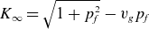 $K_{\infty } = \sqrt {1 + p_{\!f}^2} - v_g p_{\!f}$
by the expression
$K_{\infty } = \sqrt {1 + p_{\!f}^2} - v_g p_{\!f}$
by the expression $\Delta K^{\infty }_0 = \sqrt {1 + p_{\!f}^2} - v_g p_{\!f} - 1$
. Here,
$\Delta K^{\infty }_0 = \sqrt {1 + p_{\!f}^2} - v_g p_{\!f} - 1$
. Here, $p_{\!f}$
is the final longitudinal momentum of the electron and the upper time limit
$p_{\!f}$
is the final longitudinal momentum of the electron and the upper time limit $t \to \infty$
denotes a sufficiently long time such that the ponderomotive potential no longer influences the electron. Alternatively, in terms of the electron final velocity
$t \to \infty$
denotes a sufficiently long time such that the ponderomotive potential no longer influences the electron. Alternatively, in terms of the electron final velocity $v_{\!f}$
, we obtain
$v_{\!f}$
, we obtain
 \begin{equation} \Delta K^{\infty }_0 = \frac {1 - v_g v_{\!f}}{\sqrt {1 - v_{\!f}^2}} - 1, \end{equation}
which exhibits a right-skewed U-shaped profile when plotted for $-1 \leqslant v_{\!f} \leqslant 1$
. It intersects the
$-1 \leqslant v_{\!f} \leqslant 1$
. It intersects the $\Delta K^{\infty }_0 = 0$
line at two familiar points,
$\Delta K^{\infty }_0 = 0$
line at two familiar points, $v_{f,\text{no RR}} = 0$
and
$v_{f,\text{no RR}} = 0$
and $v_{f,\text{no RR}} = 2/(v_{\phi } + v_g)$
, corresponding exactly to the scattering velocities predicted by the RR-free model, when
$v_{f,\text{no RR}} = 2/(v_{\phi } + v_g)$
, corresponding exactly to the scattering velocities predicted by the RR-free model, when $K$
remains conserved. A single global minimum occurs at
$K$
remains conserved. A single global minimum occurs at $v_{\!f} = v_g$
and the sign of
$v_{\!f} = v_g$
and the sign of $\Delta K^{\infty }_0$
ultimately indicates the outcome of the electron’s motion.
$\Delta K^{\infty }_0$
ultimately indicates the outcome of the electron’s motion.
We see from (3.3) that, when $\Delta K^{\infty }_0 \lt 0$
, there are two possible positive final velocities: one smaller than
$\Delta K^{\infty }_0 \lt 0$
, there are two possible positive final velocities: one smaller than $v_g$
, which arises when the potential amplitude lies below the critical value, and one greater, occurring when the amplitude exceeds this threshold. In this latter case, the final velocity of the electron is still lower than that predicted by the RR-free model because, plotted for
$v_g$
, which arises when the potential amplitude lies below the critical value, and one greater, occurring when the amplitude exceeds this threshold. In this latter case, the final velocity of the electron is still lower than that predicted by the RR-free model because, plotted for $v_{\!f}, \Delta K^{\infty }_0$
is increasing in the efficient acceleration regime (
$v_{\!f}, \Delta K^{\infty }_0$
is increasing in the efficient acceleration regime ( $v_{\!f}\gt v_g$
).
$v_{\!f}\gt v_g$
).
When $\Delta K^{\infty }_0 \gt 0$
, there are also two mathematically possible final velocities: one exceeding
$\Delta K^{\infty }_0 \gt 0$
, there are also two mathematically possible final velocities: one exceeding $v_{f\text{no RR}}$
and one negative corresponding to a new reflection regime. The occurrence of such a reversal in the direction of the electron’s motion is a well-known effect of radiation reaction, regarded as one of its signatures when the electron interacts with electromagnetic pulses (Di Piazza, Hatsagortsyan & Keitel Reference Di Piazza, Hatsagortsyan and Keitel2009).
$v_{f\text{no RR}}$
and one negative corresponding to a new reflection regime. The occurrence of such a reversal in the direction of the electron’s motion is a well-known effect of radiation reaction, regarded as one of its signatures when the electron interacts with electromagnetic pulses (Di Piazza, Hatsagortsyan & Keitel Reference Di Piazza, Hatsagortsyan and Keitel2009).
The quantity $\Delta K_0^\infty$
captures, in a single number, the cumulative dissipative effect of the RR force over the full interaction between the electron and the electromagnetic wave. Acting essentially as a drag force, RR reduces the electron’s instantaneous velocity relative to the RR-free model. In the subcritical amplitude regime, this drag prevents the electron from remaining close to the pulse envelope, effectively shortening the interaction time with the accelerating field. As a result, a net energy gain may occur and the final velocity is no longer constrained to equal the initial one, in contrast with the RR-free case where conservation of
$\Delta K_0^\infty$
captures, in a single number, the cumulative dissipative effect of the RR force over the full interaction between the electron and the electromagnetic wave. Acting essentially as a drag force, RR reduces the electron’s instantaneous velocity relative to the RR-free model. In the subcritical amplitude regime, this drag prevents the electron from remaining close to the pulse envelope, effectively shortening the interaction time with the accelerating field. As a result, a net energy gain may occur and the final velocity is no longer constrained to equal the initial one, in contrast with the RR-free case where conservation of $K$
enforces this restriction. By contrast, in the supercritical regime, the interaction becomes sufficiently prolonged for efficient acceleration to take place (
$K$
enforces this restriction. By contrast, in the supercritical regime, the interaction becomes sufficiently prolonged for efficient acceleration to take place ( $v_{\!f} \gt v_g$
). Even in this case, however, the RR remains a dissipative force, leading to a final velocity slightly lower than in the RR-free scenario.
$v_{\!f} \gt v_g$
). Even in this case, however, the RR remains a dissipative force, leading to a final velocity slightly lower than in the RR-free scenario.
The influence of RR on the critical amplitude can also be understood by considering when an electron, initially at rest, reaches the group velocity at the peak of the potential envelope, thereby ensuring that the electron is continuously driven forward without traversing the entire wave packet. This condition corresponds to $\dot {x} = v_g$
at the instant
$\dot {x} = v_g$
at the instant $t^*$
such that
$t^*$
such that $x(t^*) - v_g t^* = 0$
. Substituting this condition into the expression for
$x(t^*) - v_g t^* = 0$
. Substituting this condition into the expression for $\Delta K^{t}_{0}$
yields
$\Delta K^{t}_{0}$
yields $\Delta K_{0}^* = -v_g p^* + \sqrt {1 + p^{*2} + a_{\text{c,RR}}^2} - 1,$
where
$\Delta K_{0}^* = -v_g p^* + \sqrt {1 + p^{*2} + a_{\text{c,RR}}^2} - 1,$
where $a_{\text{c,RR}}$
is the critical amplitude in the consideration of the RR case and
$a_{\text{c,RR}}$
is the critical amplitude in the consideration of the RR case and $p^{*}$
is the longitudinal particle’s momentum at time
$p^{*}$
is the longitudinal particle’s momentum at time $t=t^{*}$
. Using the fact that the critical amplitude in the RR-free model is known, we can precisely write
$t=t^{*}$
. Using the fact that the critical amplitude in the RR-free model is known, we can precisely write
 \begin{equation} a_{\text{c,RR}} = a_{\text{c,no RR}} \sqrt {1+ \xi \: v_\phi ^2}, \end{equation}
where $\xi =\Delta K^*_0(2+\Delta K^*_0)$
. When examining expression (3.4), we observe that there is a mathematical possibility for
$\xi =\Delta K^*_0(2+\Delta K^*_0)$
. When examining expression (3.4), we observe that there is a mathematical possibility for $\sqrt {1+ \xi \: v_\phi ^2}$
to be greater than, equal to or less than 1. If greater than 1, corresponding to
$\sqrt {1+ \xi \: v_\phi ^2}$
to be greater than, equal to or less than 1. If greater than 1, corresponding to $ \xi \gt 0$
, the effect of RR would be to increase the critical amplitude, a less favourable scenario for electron acceleration. However, if less than 1, associated with
$ \xi \gt 0$
, the effect of RR would be to increase the critical amplitude, a less favourable scenario for electron acceleration. However, if less than 1, associated with $\xi \lt 0$
, the opposite effect would occur: the critical amplitude predicted by the model that includes RR would be smaller than that obtained in the RR-free model, thus favouring efficient electron acceleration.
$\xi \lt 0$
, the opposite effect would occur: the critical amplitude predicted by the model that includes RR would be smaller than that obtained in the RR-free model, thus favouring efficient electron acceleration.
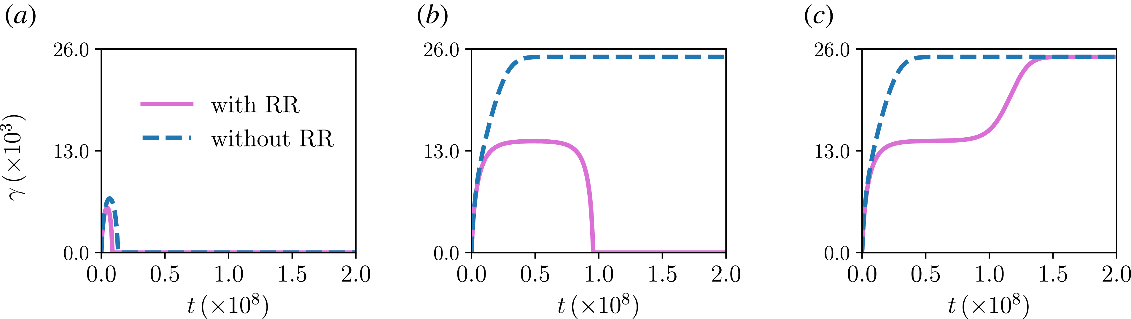
To search for these occurrences, we present in figure 1 the energy profiles resulting from the numerical integration of the equations of motion (2.4) and (2.5), associated with the Hamiltonian (3.2) and using the simplified form of the longitudinal RR force as presented in (3.1). All numerical simulations performed in this (and the next) section use $\sigma =1000$
for the carrier wave envelope length. The electron is always initially considered to be at rest in the laboratory frame of reference and very far (
$\sigma =1000$
for the carrier wave envelope length. The electron is always initially considered to be at rest in the laboratory frame of reference and very far ( $x(t=0)=6\sigma$
) from the origin on the longitudinal axis where the pulse emerges. The parameter
$x(t=0)=6\sigma$
) from the origin on the longitudinal axis where the pulse emerges. The parameter $\tau$
is directly related to the wavenumber/wavelength of the carrier wave through
$\tau$
is directly related to the wavenumber/wavelength of the carrier wave through $\tau = c \tau _0 k=2\pi c\tau _0/\lambda$
.
$\tau = c \tau _0 k=2\pi c\tau _0/\lambda$
.
Electron’s energy versus time. All panels share the parameters $v_g = 0.99996$
(
$v_g = 0.99996$
( $\gamma _g=111.805$
),
$\gamma _g=111.805$
), $\sigma = 1000$
and
$\sigma = 1000$
and $\tau = 1.5 \times 10^{-8}$
. The dashed blue curves are the prediction of the RR-free theory, while the solid one (in pink) considers RR. (a)
$\tau = 1.5 \times 10^{-8}$
. The dashed blue curves are the prediction of the RR-free theory, while the solid one (in pink) considers RR. (a) $a_0=100.000$
, (b)
$a_0=100.000$
, (b) $a_0=130.146$
, (c)
$a_0=130.146$
, (c) $a_0=130.147$
.
$a_0=130.147$
.
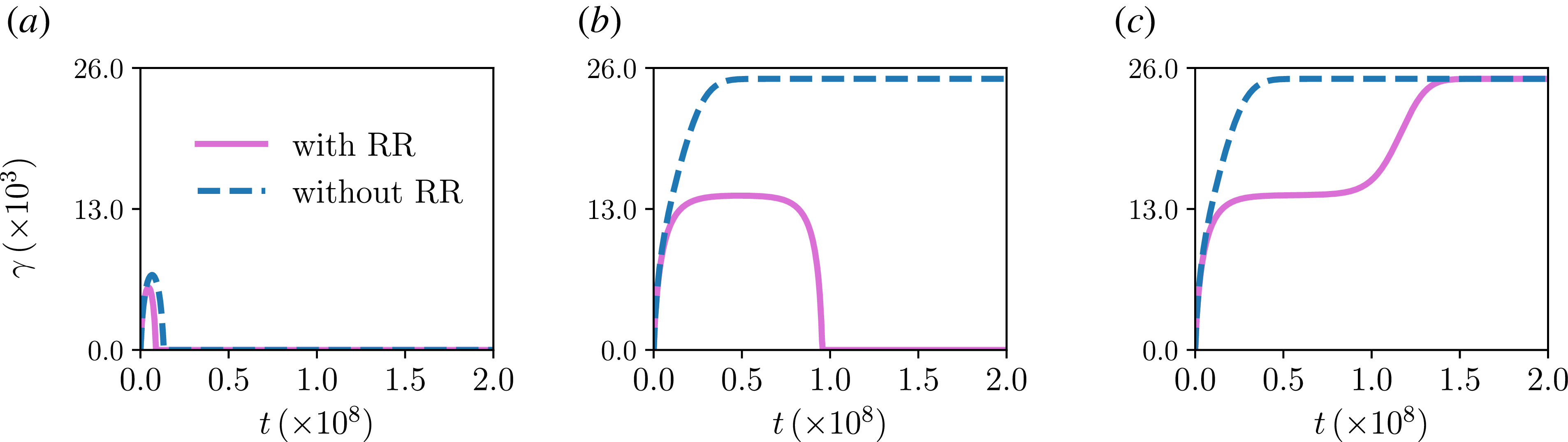
Figures 1(b) and 1(c) indicate a critical amplitude of $a_0 = 130.147$
and a corresponding final energy of approximately
$a_0 = 130.147$
and a corresponding final energy of approximately $\gamma _f = 24\,996.0$
. In these panels, we use
$\gamma _f = 24\,996.0$
. In these panels, we use $\tau = 1.5\times 10^{-8}$
, which corresponds to
$\tau = 1.5\times 10^{-8}$
, which corresponds to $\lambda \sim 0.8 \ \unicode{x03BC} \mathrm{m}$
. We know, for an electromagnetic wave propagating with group velocity
$\lambda \sim 0.8 \ \unicode{x03BC} \mathrm{m}$
. We know, for an electromagnetic wave propagating with group velocity $0.99996c$
in a cold, highly underdense plasma, that the critical amplitude predicted by the RR-free model is approximately
$0.99996c$
in a cold, highly underdense plasma, that the critical amplitude predicted by the RR-free model is approximately $a_{\text{c,no RR}} = 111.8$
and the final electron energy (once initially at rest) is approximately
$a_{\text{c,no RR}} = 111.8$
and the final electron energy (once initially at rest) is approximately $\gamma _{\text{f,no RR}} = 24\,999.5$
. This 17 % increase in the critical amplitude indicates the breakdown of conservation to which we draw attention. Also, we observed that including radiation reaction reduces the final electron energy by approximately 0.014 % when the carrier wave potential amplitude is critical.
$\gamma _{\text{f,no RR}} = 24\,999.5$
. This 17 % increase in the critical amplitude indicates the breakdown of conservation to which we draw attention. Also, we observed that including radiation reaction reduces the final electron energy by approximately 0.014 % when the carrier wave potential amplitude is critical.
To establish a connection between the specific cases discussed previously and the analysis of the $K$
conservation breakdown, we present in figure 2 the values of
$K$
conservation breakdown, we present in figure 2 the values of $\Delta K^{\infty }_{0}$
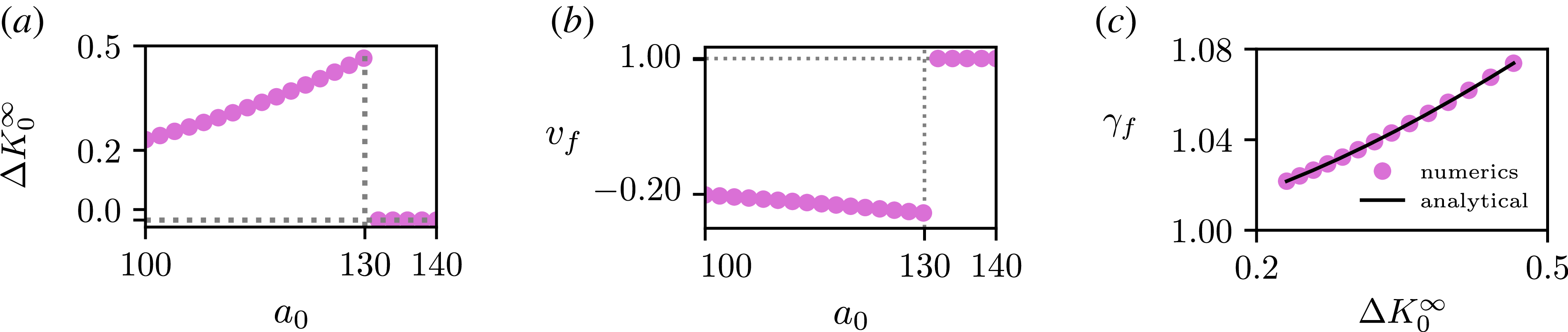
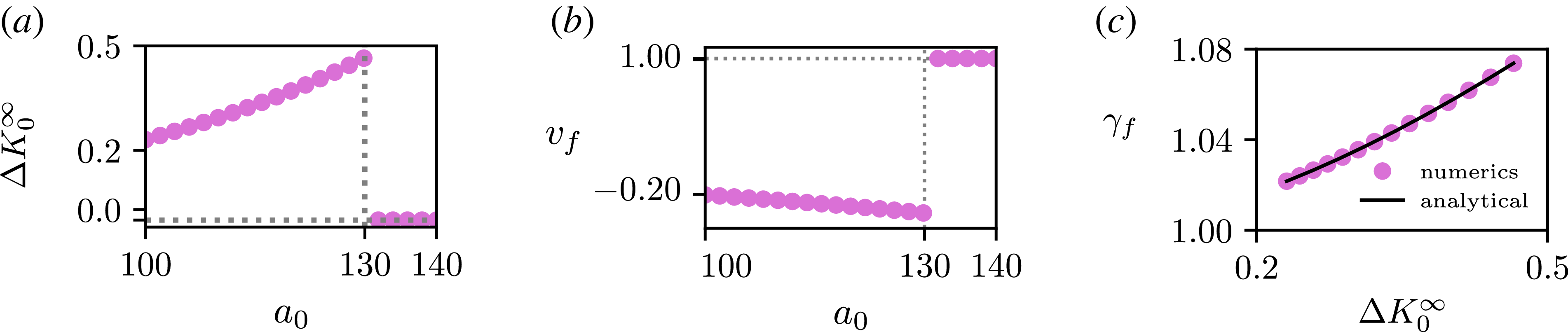
for an electron interacting with pulses of fixed wavelengths and variable amplitudes, as well as the corresponding ejection velocities. Each point in the panels represents the final result of a complete simulation done by integrating the same equations as in figure 1. Figure 2(a) shows that
$\Delta K^{\infty }_{0}$
for an electron interacting with pulses of fixed wavelengths and variable amplitudes, as well as the corresponding ejection velocities. Each point in the panels represents the final result of a complete simulation done by integrating the same equations as in figure 1. Figure 2(a) shows that $\Delta K^{\infty }_{0}$
, obtained via direct numerical integration along the solution of the Hamiltonian system, changes its sign from positive to negative as the amplitude in the simulation transits from below to above the critical amplitude value. This discontinuity precisely marks the transition between the reflection and efficient acceleration regimes, as shown in figure 2(b). The efficient acceleration regime is characterised by a plateau where
$\Delta K^{\infty }_{0}$
, obtained via direct numerical integration along the solution of the Hamiltonian system, changes its sign from positive to negative as the amplitude in the simulation transits from below to above the critical amplitude value. This discontinuity precisely marks the transition between the reflection and efficient acceleration regimes, as shown in figure 2(b). The efficient acceleration regime is characterised by a plateau where $\Delta K^{\infty }_{0} \lt 0$
. Each point in figure 2(c) corresponds to a numerical solution obtained for a fixed value of
$\Delta K^{\infty }_{0} \lt 0$
. Each point in figure 2(c) corresponds to a numerical solution obtained for a fixed value of $a_0$
, varied within the range
$a_0$
, varied within the range $100 \leqslant a_0 \leqslant 130 \leqslant a_{\text{c,RR}}$
, while the continuous black curve represents the analytical prediction given by (3.3). We can see an excellent agreement between the numerical simulations and the analytical prediction when
$100 \leqslant a_0 \leqslant 130 \leqslant a_{\text{c,RR}}$
, while the continuous black curve represents the analytical prediction given by (3.3). We can see an excellent agreement between the numerical simulations and the analytical prediction when $\Delta K^{\infty }_{0}$
is directly compared with the electron’s ejection energy.
$\Delta K^{\infty }_{0}$
is directly compared with the electron’s ejection energy.
Panel (a) displays the evolution of $\Delta K_{0}^{\infty }$
versus the potential amplitude, whereas panel (b) presents, for comparison, the corresponding ejection velocity of the electron. Panel (c) shows the evolution of
$\Delta K_{0}^{\infty }$
versus the potential amplitude, whereas panel (b) presents, for comparison, the corresponding ejection velocity of the electron. Panel (c) shows the evolution of $\Delta K_{0}^{\infty }$
versus the final energy
$\Delta K_{0}^{\infty }$
versus the final energy $\gamma _f$
, both numerical and analytical predictions to
$\gamma _f$
, both numerical and analytical predictions to $a_0\lt a_{\text{c,RR}}$
. The comparison highlights the connection between these quantities. Parameters adopted:
$a_0\lt a_{\text{c,RR}}$
. The comparison highlights the connection between these quantities. Parameters adopted: $\sigma = 10^3$
,
$\sigma = 10^3$
, $v_g = 0.99996$
, fixed
$v_g = 0.99996$
, fixed $\tau =1.5\times 10^{-8}$
and circular polarisation.
$\tau =1.5\times 10^{-8}$
and circular polarisation.
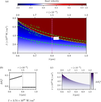
To provide an overview of the accessible dynamical regimes, figure 3(a) displays a colour map of the electron ejection velocity as a function of the carrier wave intensity ( $I$
) and its wavelength (
$I$
) and its wavelength ( $\lambda$
). The latter is directly related to the parameter
$\lambda$
). The latter is directly related to the parameter $\tau$
shown along the top axis. The intensity (in
$\tau$
shown along the top axis. The intensity (in $10^{22}$
W cm
$10^{22}$
W cm $^{-2}$
) relates to the wavelength (in microns) and the amplitude parameter
$^{-2}$
) relates to the wavelength (in microns) and the amplitude parameter $a_0$
through the relation
$a_0$
through the relation $I\,\lambda _{\unicode{x03BC}\rm m}^2 \approx 1.37\,a_0^2$
. This relation enables the superposition of constant-
$I\,\lambda _{\unicode{x03BC}\rm m}^2 \approx 1.37\,a_0^2$
. This relation enables the superposition of constant- $a_0$
curves corresponding to different intensity–wavelength combinations, as illustrated in figure 3(a) by the dashed green curves labelled with their respective
$a_0$
curves corresponding to different intensity–wavelength combinations, as illustrated in figure 3(a) by the dashed green curves labelled with their respective $a_0$
values.
$a_0$
values.
Panel (a) presents the complete electron ejection velocity map. The dashed curves indicate different combinations of laser intensity $I$
and wavelength
$I$
and wavelength $\lambda$
corresponding to a fixed normalised vector potential
$\lambda$
corresponding to a fixed normalised vector potential $a_0$
. Panel (b) displays the evolution of
$a_0$
. Panel (b) displays the evolution of $\Delta K^{\infty }_0$
for fixed intensity
$\Delta K^{\infty }_0$
for fixed intensity $I$
and varying wavelength
$I$
and varying wavelength $\lambda$
. Panel (c) maps
$\lambda$
. Panel (c) maps $\Delta K^{\infty }_0$
onto the same sets of
$\Delta K^{\infty }_0$
onto the same sets of $(I,\lambda )$
combinations as shown in panel (a). Parameters:
$(I,\lambda )$
combinations as shown in panel (a). Parameters: $\sigma = 10^3$
and
$\sigma = 10^3$
and $v_g = 0.99996$
.
$v_g = 0.99996$
.
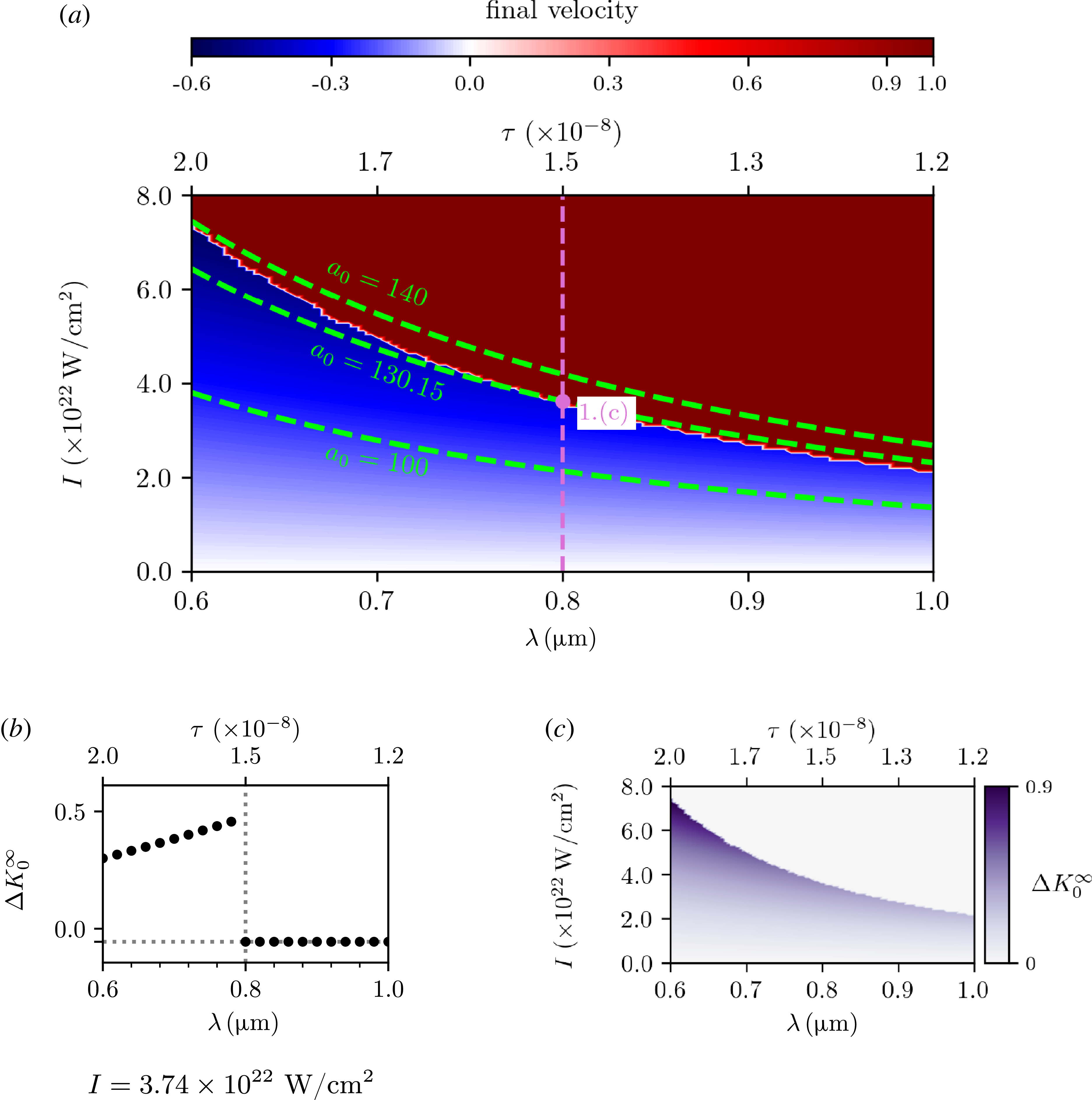
Three distinct regions emerge: the transmission region (white), where the electron exhibits no net energy gain; the reflection region (dark blue), where the electron is reflected by the wave; and the efficient acceleration region (dark red), where the electron reaches velocities exceeding the group velocity of the wave. The vertical dashed orchid line corresponds to the parameters used in figure 1. The point labelled ‘1(c)’ indicates the critical value of $a_0$
at which the transition to efficient acceleration occurs as the wave intensity is increased for a fixed
$a_0$
at which the transition to efficient acceleration occurs as the wave intensity is increased for a fixed $\lambda =0.8 \ \unicode{x03BC}$
m.
$\lambda =0.8 \ \unicode{x03BC}$
m.
The observed behaviour is directly associated with the breakdown of the conservation of $K$
, as illustrated in figure 3(b), where
$K$
, as illustrated in figure 3(b), where $\Delta K^{\infty }_{0}$
is evaluated numerically from its defining integral. Each point corresponds to a simulation at fixed intensity
$\Delta K^{\infty }_{0}$
is evaluated numerically from its defining integral. Each point corresponds to a simulation at fixed intensity $I$
, while the dissipation parameter is varied. For smaller values of
$I$
, while the dissipation parameter is varied. For smaller values of $\lambda$
(i.e. larger
$\lambda$
(i.e. larger $\tau$
),
$\tau$
), $\Delta K^{\infty }_{0}$
remains positive, characterising the reflection regime. As
$\Delta K^{\infty }_{0}$
remains positive, characterising the reflection regime. As $\lambda$
increases (equivalently,
$\lambda$
increases (equivalently, $\tau$
decreases), a discontinuity emerges at the value corresponding to the critical condition. Beyond this point,
$\tau$
decreases), a discontinuity emerges at the value corresponding to the critical condition. Beyond this point, $\Delta K^{\infty }_{0}$
becomes slightly negative and progressively decreases, signalling the transition to the efficient acceleration regime.
$\Delta K^{\infty }_{0}$
becomes slightly negative and progressively decreases, signalling the transition to the efficient acceleration regime.
This relation between the change in the acceleration scenario and the violation of the conservation of $K$
is also evident in figure 3(c), which shows a map of the values of
$K$
is also evident in figure 3(c), which shows a map of the values of $\Delta K _0^\infty$
for the same combinations of intensity and wavelength (or RR significance) as in figure 3(a). While the system is in the reflection region, characterised by very dark purple shades, the values of
$\Delta K _0^\infty$
for the same combinations of intensity and wavelength (or RR significance) as in figure 3(a). While the system is in the reflection region, characterised by very dark purple shades, the values of $\Delta K_{0}^{\infty }$
are positive. However, once the
$\Delta K_{0}^{\infty }$
are positive. However, once the $\lambda$
values enter the region associated with efficient acceleration, it attains a slightly negative value, consistent with the behaviour described previously.
$\lambda$
values enter the region associated with efficient acceleration, it attains a slightly negative value, consistent with the behaviour described previously.
The parameter regime explored here, characterised by $\lambda \sim 0.8\,\unicode{x03BC} \text{m}$
and
$\lambda \sim 0.8\,\unicode{x03BC} \text{m}$
and $a_0 \sim 100$
, is compatible with present-day laser systems (Mourou et al. Reference Mourou, Mironov, Khazanov and Sergeev2014; Danson, Haefner & Bromage Reference Danson2019). Experimental demonstrations have already achieved peak intensities of up to
$a_0 \sim 100$
, is compatible with present-day laser systems (Mourou et al. Reference Mourou, Mironov, Khazanov and Sergeev2014; Danson, Haefner & Bromage Reference Danson2019). Experimental demonstrations have already achieved peak intensities of up to $10^{22}{-}10^{23}\,\rm{W\,cm}^{-2}$
(Yoon, Jeon & Shin Reference Yoon2021), ensuring that the regimes analysed here are experimentally accessible.
$10^{22}{-}10^{23}\,\rm{W\,cm}^{-2}$
(Yoon, Jeon & Shin Reference Yoon2021), ensuring that the regimes analysed here are experimentally accessible.
3.2. Linear polarisation
In the case of $y$
-linear polarisation, we set
$y$
-linear polarisation, we set $\epsilon = 1$
in (2.1) and recalculate the RR force from (2.2). Once again, our model neglects transverse contributions and terms that can be reasonably disregarded. In this set-up, detailed calculations are provided in Appendix A.2, the longitudinal component of the RR force takes the form
$\epsilon = 1$
in (2.1) and recalculate the RR force from (2.2). Once again, our model neglects transverse contributions and terms that can be reasonably disregarded. In this set-up, detailed calculations are provided in Appendix A.2, the longitudinal component of the RR force takes the form
 \begin{equation} g_{\textrm {RR}_x} = g_{\textrm {RR}_x}^{(2)} \ \ a_0^2e^{-{2(({(x-v_g\,t)^2})/{\sigma ^2})}}+ g_{\textrm {RR}_x}^{(4)} \ \ a_0^4e^{-{4(({(x-v_g\,t)^2})/{\sigma ^2})}}, \end{equation}
where the coefficients are
 \begin{align} g_{\textrm {RR}_x}^{(2)} &=2\tau \ \left (v_\phi -\frac {p}{\gamma }\right )\left [1 - p \ \gamma \left (v_{\phi } - \frac {p}{\gamma }\right )\cos ^2\theta \right ], \nonumber\\ g_{\textrm {RR}_x}^{(4)}&=\tau \ (v_\phi ^2-1) \frac {p}{\gamma } \ \sin ^2 2\theta , \end{align}
and the Hamiltonian presents as
 \begin{equation} H_{\textit{lin}} = \sqrt {1+p^2+a_0^2e^{ -{(({2( \overline x-v_g\,t)^2 })/{ \sigma ^2})}}(1-\cos 2\theta )}, \end{equation}
where $p$
is the electron’s longitudinal momentum.
$p$
is the electron’s longitudinal momentum.
Unlike the circular polarisation case, the longitudinal RR force component (3.5) – as well as the Hamiltonian itself – does not exhibit a natural suppression of high-frequency $\theta$
-jitter terms. Therefore, we adopt the canonical ponderomotive approach as developed by Russman et al. (Reference Russman, Marini and Rizzato2022), with the addition of a final time-averaging procedure aimed at filtering out the high-frequency oscillations introduced by the RR terms, similarly as we did previously (Russman et al. Reference Russman, Almansa, Peter, Marini and Rizzato2020).
$\theta$
-jitter terms. Therefore, we adopt the canonical ponderomotive approach as developed by Russman et al. (Reference Russman, Marini and Rizzato2022), with the addition of a final time-averaging procedure aimed at filtering out the high-frequency oscillations introduced by the RR terms, similarly as we did previously (Russman et al. Reference Russman, Almansa, Peter, Marini and Rizzato2020).
In the absence of the RR force, we seek canonical variables $\overline x$
and
$\overline x$
and $\overline p$
, the centre of oscillation motion and its momentum, which are free from fast time-scale dependencies. These slow variables are defined by
$\overline p$
, the centre of oscillation motion and its momentum, which are free from fast time-scale dependencies. These slow variables are defined by $\overline x = x + \partial f/ \partial \overline p$
and
$\overline x = x + \partial f/ \partial \overline p$
and $\overline p = p - \partial f/\partial x$
, while the transformation is performed by the generator function
$\overline p = p - \partial f/\partial x$
, while the transformation is performed by the generator function $F(x,\overline p , t) = x \; \overline p + f( x, \overline p, t)$
, where the function
$F(x,\overline p , t) = x \; \overline p + f( x, \overline p, t)$
, where the function
 \begin{equation} f(x,\overline p,t) =\frac {a_0^2}{4} \frac{ e^{ -(({2( x-v_g\,t)^2})/{ \sigma ^2})}}{ \, (\overline p - v_\phi \varGamma )\,} \sin 2 \theta , \quad \mbox{with} \ \ \varGamma =\sqrt {1+\overline p^2 + a_0^2e^{ -{(({2( \overline x-v_g\,t)^2})/{ \sigma ^2})}}}, \end{equation}
comprises the $\theta$
dependence. The Hamiltonian transforms as
$\theta$
dependence. The Hamiltonian transforms as ${\overline H}_{lin} = H_{lin} + \partial f/ \partial t$
, being its low-frequency canonical version given by
${\overline H}_{lin} = H_{lin} + \partial f/ \partial t$
, being its low-frequency canonical version given by
 \begin{equation} {\overline H}_{lin} = \sqrt {1+\overline p^2 + a_0^2e^{ -{(({2( \overline x-v_g\,t)^2})/{ \sigma ^2})}} - \frac {v_\phi ^2-1}{8( \overline p - v_\phi \varGamma )^2} a_0^4 e^{-(({{4 (\overline x-v_g t)^2}})/{\sigma ^2})}}. \end{equation}
Once the RR force is introduced, the canonical equations in the new slow longitudinal motion variables are subject to a modification, namely
 \begin{equation} \dot {\overline p} = - \frac {\partial {\overline H}_{\textit{lin}}}{ \partial \overline x} + \left \langle \frac {g_{\text{RR}_x}}{1+(({\partial ^2 f})/({\partial x \partial \overline p}))} \right \rangle _{\theta } \end{equation}
and
 \begin{equation} \dot {\overline {x}} = \frac {\partial \overline {H}_{\textit{lin}}}{\partial \overline {p}} + \left \langle \frac {g_{\text{RR}_x} }{1 + (({\partial ^2 f})/({\partial x \partial \overline {p}}))}\frac {\partial ^2 f}{\partial \overline {p}^2} \right \rangle _{\theta }. \end{equation}
We define the fast-time (or fast-phase) average as $ \left \langle g \right \rangle _{\theta } \equiv (2 \pi )^{-1} \oint g(\theta ) \,{\rm d}\theta$
for a generic function
$ \left \langle g \right \rangle _{\theta } \equiv (2 \pi )^{-1} \oint g(\theta ) \,{\rm d}\theta$
for a generic function $g=g(\theta )$
. To clarify how these averages were calculated, consider any smooth function
$g=g(\theta )$
. To clarify how these averages were calculated, consider any smooth function $r=r(x,p,t)$
of rapidly changing variables. The average value, up to first order, of its transformed value
$r=r(x,p,t)$
of rapidly changing variables. The average value, up to first order, of its transformed value $\tilde {r} = r(\overline {x}+\delta x, \overline {p} + \delta p,t)$
is given by
$\tilde {r} = r(\overline {x}+\delta x, \overline {p} + \delta p,t)$
is given by
 \begin{equation} \left \langle \tilde {r} \right \rangle _{\theta } = \left \langle r(\overline {x},\overline {p},t)\right \rangle _{\theta } + \left \langle \frac {\partial r}{\partial x} \: \delta x \right \rangle _{\theta } + \left \langle \frac {\partial r}{\partial p} \: \delta p \right \rangle _{\theta }, \end{equation}
understanding that
 \begin{equation} \frac {\partial r}{\partial x} = \frac {\partial r}{\partial x} \Big |_{\substack {x=\overline {x} \\ p=\overline {p}}},\quad \frac {\partial r}{\partial p}= \frac {\partial r}{\partial p} \Big |_{\substack {x=\overline {x} \\ p=\overline {p}}} ,\quad \delta x = - \frac {\partial f}{\partial \overline {p}}\quad \mbox{and} \quad \delta p = \frac {\partial f}{\partial x}. \end{equation}
Carrying on with the calculations, we arrive at the following expression for the mean values:
 \begin{align} \left \langle \frac {g_{\text{RR}_x}}{1+({\partial ^2 f}/{\partial x \partial \overline p})} \right \rangle _{\theta } & = \left \langle \frac {g^{(2)}_{\text{RR}_x}}{1+({\partial ^2 f}/{\partial x \partial \overline p})} \right \rangle _{\theta } \ a_0^2e^{-{2(({(\overline {x}-v_g\,t)^2})/{\sigma ^2})}}\nonumber\\&\quad + \left \langle \frac {g^{(4)}_{\text{RR}_x}}{1+({\partial ^2 f}/{\partial x \partial \overline p})} \right \rangle _{\theta } \ a_0^4e^{-{4(({(\overline {x}-v_g\,t)^2})/{\sigma ^2})}}, \end{align}
where
 \begin{equation} \left \langle \frac {g^{(2)}_{\text{RR}_x}}{1+({\partial ^2 f}/\partial x \partial \overline p)} \right \rangle _{\theta }= \tau \left (v_\phi - \frac {\overline {p}}{\overline {\gamma }} \right ) \left [ 2 - \overline {\gamma } \; \overline {p} \left (v_\phi - \frac {\overline {p}}{\overline {\gamma }} \right )\right ], \end{equation}
 \begin{equation} \left \langle \frac {g^{(4)}_{\text{RR}_x}}{1+({\partial ^2 f}/{\partial x \partial \overline p})} \right \rangle _{\theta } = \tau \frac {(v_\phi ^2-1)}{2} \frac {\overline {p}}{\overline {\gamma }} + \frac {\partial b}{\partial \overline {p}}\,\varPsi (\overline {p},\overline {x}) + \frac {b + ({\partial b}/{\partial \overline {p}})}{2} \, \frac {\partial \varPsi }{\partial \overline {p}}(\overline {p},\overline {x}), \end{equation}
with $\overline {\gamma } = \sqrt {1+\overline p^2 + a_0^2e^{ -{(({2( \overline x-v_g\,t)^2})/{\sigma ^2})}} }$
,
$\overline {\gamma } = \sqrt {1+\overline p^2 + a_0^2e^{ -{(({2( \overline x-v_g\,t)^2})/{\sigma ^2})}} }$
, $\varPsi (\overline {p},\overline {x}) =-2\overline {\gamma } \; \overline {p} \; (v_\phi -({\overline {p}}/{\overline {\gamma }}))^2$
,
$\varPsi (\overline {p},\overline {x}) =-2\overline {\gamma } \; \overline {p} \; (v_\phi -({\overline {p}}/{\overline {\gamma }}))^2$
, $b(\overline {p},\overline {x})^{-1} = 8(v_\phi \overline {\gamma } - \overline {p})$
and
$b(\overline {p},\overline {x})^{-1} = 8(v_\phi \overline {\gamma } - \overline {p})$
and
 \begin{equation} \left \langle \frac {g_{\text{RR}_x} }{1 + ({\partial ^2 f}/{\partial x \partial \overline {p}})}\frac {\partial ^2 f}{\partial \overline {p}^2} \right \rangle _{\theta } = 0 . \end{equation}
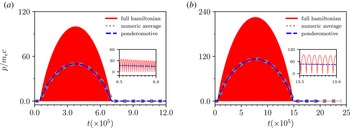
Longitudinal momentum versus time. The solid red curve represents the solution of Hamilton’s equations for the Hamiltonian given in (3.7). The dashed grey curve shows the moving-window average of the velocity obtained from the previously referenced system. The dashed blue curve corresponds to the predicted average from the canonical model. (a) $a_0=10.0$
,
$a_0=10.0$
, $\tau =1.5 \times 10^{-8}$
, (b)
$\tau =1.5 \times 10^{-8}$
, (b) $a_0=15.0$
,
$a_0=15.0$
, $\tau =1.0 \times 10^{-8}$
.
$\tau =1.0 \times 10^{-8}$
.
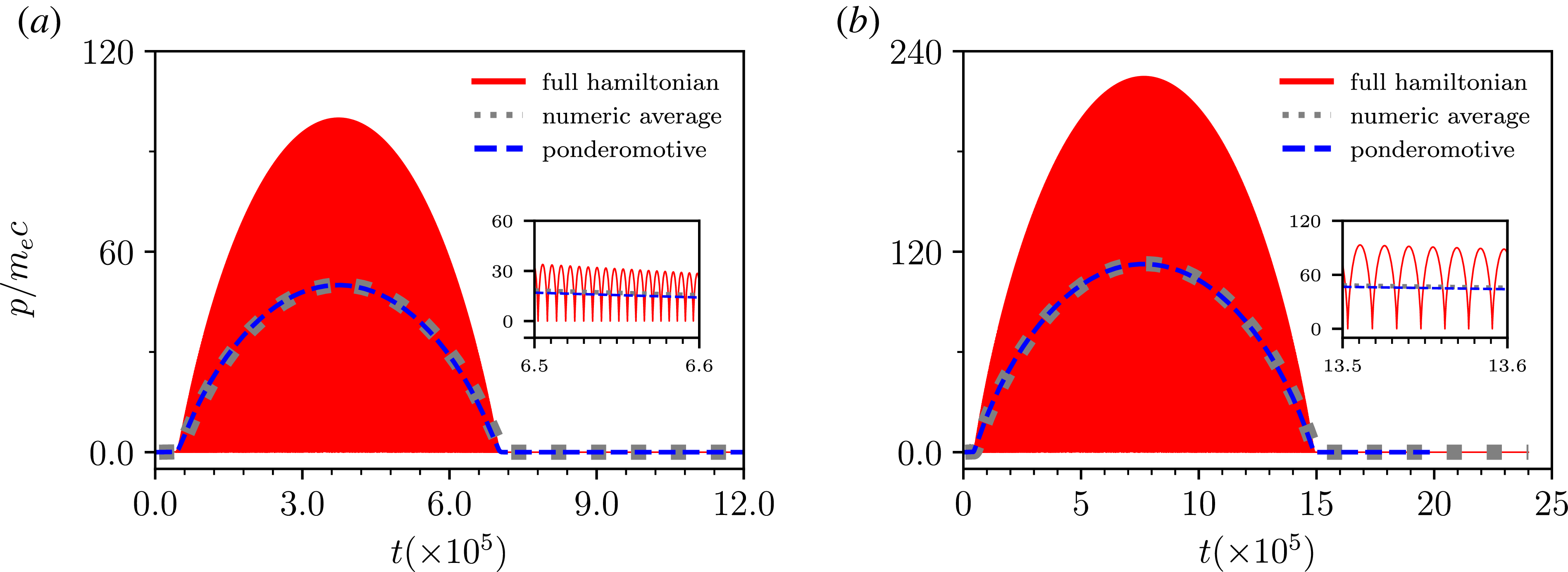
The ponderomotive Hamiltonian approach, modified to incorporate RR effects, captures the time-averaged dynamics of the particle’s longitudinal momentum with high fidelity, as illustrated in figure 4. It compares the results from the direct integration of the full Hamilton’s equations coming from the Hamiltonian (3.7) (solid red line), the numerical moving-window average of the velocity computed from the full system (grey dotted line), and the predictions from the averaged model (blue dashed line) given by (3.10) and (3.11). A strong agreement is observed in regimes where the ponderomotive approach holds, thus supporting the validity of the averaged formalism even in the presence of RR-induced dissipation. Part of the success of the description may be related to the fact that the correction in amplitude introduced by the proposed canonical formalism better predicts the transit time of the wave with the electron, as pointed out by Russman et al. (Reference Russman, Marini and Rizzato2022).
Furthermore, the averaged system exhibits a (non-)conserved-like structure analogous to that found in the case of circular polarisation. Specifically, one may define the quantity $\mathcal{K} = \overline {H}_{\textit{lin}} - v_g \overline {p}$
, whose total variation is given by
$\mathcal{K} = \overline {H}_{\textit{lin}} - v_g \overline {p}$
, whose total variation is given by
 \begin{equation} \Delta \mathcal{K}_{0}^{t} = \int _{0}^{t} (\dot {\overline {x}} - v_g) \left \langle \frac {g_{\text{RR},x}}{1 + ({\partial ^2 f}/{\partial x \partial \overline {p}})} \right \rangle _{\theta \prime} \,{\rm d}t^\prime. \end{equation}
As in the circular polarisation scenario, the electron–wave interaction can thus be interpreted in terms of the breakdown of $\mathcal{K}$
conservation, induced by energy loss via radiation and/or the direct action of the RR force. This violation enables a net energy gain by the particle, even in regimes where sustained acceleration would otherwise be forbidden in the absence of RR.
$\mathcal{K}$
conservation, induced by energy loss via radiation and/or the direct action of the RR force. This violation enables a net energy gain by the particle, even in regimes where sustained acceleration would otherwise be forbidden in the absence of RR.
4. Conclusions
The study of RR effects on the dynamics of particles accelerated by electromagnetic wave pulses, within the model employed here, reveals two major modifications relative to the RR-free case. First, the critical amplitude of the vector potential required for efficient acceleration – defined as the condition in which the electron acquires a longitudinal velocity exceeding the group velocity of the accelerating wave – becomes dependent on the packet frequency, no longer being determined solely by the wave’s group velocity. The predicted critical amplitude, when the RR is included, for a realistic combination of parameters for an accelerating electromagnetic wave ( $\lambda \sim 1\,\unicode{x03BC} \text{m}$
and
$\lambda \sim 1\,\unicode{x03BC} \text{m}$
and $I \sim 10^{22}$
W cm
$I \sim 10^{22}$
W cm $^{-2}$
) increases considerably. There is also a slight reduction in the electron’s final energy when the RR is included. The passing regime found in the RR-free theory is instead converted into a reflection regime, where the particle still experiences a net energy gain, but ends up with a final longitudinal velocity that is lower than the group velocity of the accelerating wave and directed backward.
$^{-2}$
) increases considerably. There is also a slight reduction in the electron’s final energy when the RR is included. The passing regime found in the RR-free theory is instead converted into a reflection regime, where the particle still experiences a net energy gain, but ends up with a final longitudinal velocity that is lower than the group velocity of the accelerating wave and directed backward.
The emergence of these new dynamical regimes and altered behaviours induced by RR can be understood through the breaking of the conservation of a quantity that, in the RR-free model, remains invariant.
Acknowledgements
The authors are grateful to Professor David Burton for fruitful discussions about the results arising from our analytical developments.
Editor Luís O. Silva thanks the referees for their advice in evaluating this article.
Funding
We acknowledge support from Fundação de Amparo à Pesquisa do Estado de São Paulo (FAPESP), under Grant No. 2024/03570-7, and the National Council for Scientific and Technological Development, CNPq (Grants No. 302665/2017-0 and 150825/2024-2).
Declaration of interests
The authors report no conflict of interest.
Data availability
The data that support the findings of this study are available from the corresponding author upon reasonable request.
Appendix A. RR force components
Determining the components of the RR force acting on an electron begins with specifying the vector potential, as described in (2.1). This potential is adapted for circular (Appendix A.1) and linear (Appendix A.2) polarisation, allowing the derivation of the electric ( $\boldsymbol{E}=-\partial _t\boldsymbol{A}$
) and magnetic (
$\boldsymbol{E}=-\partial _t\boldsymbol{A}$
) and magnetic ( $\boldsymbol{B}=\hat {\boldsymbol{x}} \times \partial _x\boldsymbol{A}$
) fields, assuming a vanishing scalar potential and a vector potential of the form
$\boldsymbol{B}=\hat {\boldsymbol{x}} \times \partial _x\boldsymbol{A}$
) fields, assuming a vanishing scalar potential and a vector potential of the form $\boldsymbol{A}=\boldsymbol{A}(x,t)$
. Subsequently, these fields are inserted into the general expression for the normalised radiation reaction (RR) force
$\boldsymbol{A}=\boldsymbol{A}(x,t)$
. Subsequently, these fields are inserted into the general expression for the normalised radiation reaction (RR) force
 \begin{align} \frac {1}{\tau } {\boldsymbol {g}}_{\text{RR}}&= - \gamma (\boldsymbol{\dot {E}} + \boldsymbol{v} \times \boldsymbol{\dot {B}}) + [(\boldsymbol{v} \boldsymbol{\cdot }\boldsymbol{E})\boldsymbol{E} + (\boldsymbol{E} + \boldsymbol{v} \times \boldsymbol{B}) \times \boldsymbol{B}] \nonumber\\ & \quad -\gamma ^2 [(\boldsymbol{E} + \boldsymbol{v} \times \boldsymbol{B})^2 - (\boldsymbol{v} \boldsymbol{\cdot }\boldsymbol{E})^2]\boldsymbol{v} \end{align}
to obtain its specific components.
In the relativistic regime ( $a_0 \gg 1$
), the RR force effectively acts as a drag force, as the dominant term in (A1) scales as
$a_0 \gg 1$
), the RR force effectively acts as a drag force, as the dominant term in (A1) scales as $\gamma ^2$
and is aligned with the instantaneous electron velocity, i.e. with its momentum. The cycle-averaged momentum in this regime is strongly anisotropic: the longitudinal component scales as
$\gamma ^2$
and is aligned with the instantaneous electron velocity, i.e. with its momentum. The cycle-averaged momentum in this regime is strongly anisotropic: the longitudinal component scales as $a_0^2$
, whereas the transverse component scales as
$a_0^2$
, whereas the transverse component scales as $a_0$
(See Chapter 3 of Gibbon Reference Gibbon2005, for example; or Pukhov Reference Pukhov2003), yielding
$a_0$
(See Chapter 3 of Gibbon Reference Gibbon2005, for example; or Pukhov Reference Pukhov2003), yielding $p_x \gg p_\perp$
. Consequently, upon averaging over the fast oscillations, the RR force acts predominantly along the longitudinal direction. Hence, in the central region of the pulse, where the envelope varies slowly and efficient acceleration occurs, the dynamics is essentially governed by the longitudinal component of the RR force, which is the focus of the present model.
$p_x \gg p_\perp$
. Consequently, upon averaging over the fast oscillations, the RR force acts predominantly along the longitudinal direction. Hence, in the central region of the pulse, where the envelope varies slowly and efficient acceleration occurs, the dynamics is essentially governed by the longitudinal component of the RR force, which is the focus of the present model.
A.1. Circular polarisation
Particularising the vector potential (2.1) for circular polarisation, we have $\boldsymbol{A}_{\textit{circ}}= A_y \ \hat{\!\boldsymbol{y}}+A_z \ \hat {\boldsymbol{z}}$
, where
$\boldsymbol{A}_{\textit{circ}}= A_y \ \hat{\!\boldsymbol{y}}+A_z \ \hat {\boldsymbol{z}}$
, where $A_y = A_0(x,t)\sin \theta$
and
$A_y = A_0(x,t)\sin \theta$
and $A_z =A_0(x,t)\cos \theta$
, once the modulated amplitude function is defined as
$A_z =A_0(x,t)\cos \theta$
, once the modulated amplitude function is defined as
 \begin{equation} A_0(x,t) = a_0 \exp {\left (-{\frac {(x-v_g\,t)^2}{\sigma ^2}}\right )}. \end{equation}
To obtain a version of the RR force (A1) that is more amenable to analytical treatment, several considerations are pertinent. First, the partial derivatives of the envelope function (A2) contain a factor of $1/ \sigma ^{2}$
, which, under conditions of slow modulation (
$1/ \sigma ^{2}$
, which, under conditions of slow modulation ( $\sigma \gg 1$
), causes them to exhibit adiabatic growth. Furthermore, the various products that arise from these derivatives within the RR force, such as
$\sigma \gg 1$
), causes them to exhibit adiabatic growth. Furthermore, the various products that arise from these derivatives within the RR force, such as $A_0 \partial _x A_0^2$
for example, have an additional factor
$A_0 \partial _x A_0^2$
for example, have an additional factor $\tau \ll 1$
. When comparing scales, it is observed that these products in (A2) scale, at maximum, with
$\tau \ll 1$
. When comparing scales, it is observed that these products in (A2) scale, at maximum, with $\tau /\sigma ^2$
. In contrast, the Lorentz force scales only with
$\tau /\sigma ^2$
. In contrast, the Lorentz force scales only with $1/\sigma ^{2}$
. Thus, the contribution of terms in the RR force that contain partial derivatives becomes negligible when compared with the Lorentz force. Consequently, to simplify the modelling, our approach will retain only those terms of the RR force involving powers of
$1/\sigma ^{2}$
. Thus, the contribution of terms in the RR force that contain partial derivatives becomes negligible when compared with the Lorentz force. Consequently, to simplify the modelling, our approach will retain only those terms of the RR force involving powers of $A_0$
, disregarding those involving its partial derivatives.
$A_0$
, disregarding those involving its partial derivatives.
This can be achieved by choosing $\partial _x A_y = A_z$
,
$\partial _x A_y = A_z$
, $\partial _x A_z = -A_y$
,
$\partial _x A_z = -A_y$
, $\partial _t A_y = -v_{\phi } A_z$
and
$\partial _t A_y = -v_{\phi } A_z$
and $\partial _t A_z = v_{\phi } A_y$
; that is, by representing it as a plane circularly polarised carrier wave with constant amplitude. From these relations, the electric and magnetic fields are readily obtained as
$\partial _t A_z = v_{\phi } A_y$
; that is, by representing it as a plane circularly polarised carrier wave with constant amplitude. From these relations, the electric and magnetic fields are readily obtained as $\boldsymbol{E} = v_\phi (A_z \, \hat{\boldsymbol{y}} - A_y \, \hat{\boldsymbol{z}})$
and
$\boldsymbol{E} = v_\phi (A_z \, \hat{\boldsymbol{y}} - A_y \, \hat{\boldsymbol{z}})$
and $\boldsymbol{B} = \boldsymbol{A}_{\textit{circ}}$
. It then follows that
$\boldsymbol{B} = \boldsymbol{A}_{\textit{circ}}$
. It then follows that $\dot {\boldsymbol{E}} = v_\phi (v_\phi - \dot {x})\,\boldsymbol{A}_{\textit{circ}}$
and
$\dot {\boldsymbol{E}} = v_\phi (v_\phi - \dot {x})\,\boldsymbol{A}_{\textit{circ}}$
and $\dot {\boldsymbol{B}} =(v_\phi - \dot {x})(-A_z \hat {\boldsymbol{ y}} + A_y \hat {\boldsymbol{z}})$
.
$\dot {\boldsymbol{B}} =(v_\phi - \dot {x})(-A_z \hat {\boldsymbol{ y}} + A_y \hat {\boldsymbol{z}})$
.
The first term of (A1), therefore, using $\boldsymbol{v}=\dot {x} \ \hat {\boldsymbol{x}}+\dot {y} \ \hat{\!\boldsymbol{y}}+\dot {z} \ \hat {\boldsymbol{z}}$
, has a longitudinal component proportional to
$\boldsymbol{v}=\dot {x} \ \hat {\boldsymbol{x}}+\dot {y} \ \hat{\!\boldsymbol{y}}+\dot {z} \ \hat {\boldsymbol{z}}$
, has a longitudinal component proportional to
 \begin{equation} \begin{split} [\dot {\boldsymbol{E}} + \boldsymbol{v}\times \boldsymbol{\dot {B}}]_x &=(v_\phi - \dot {x}) (\dot {y} A_y + \dot {z} A_z). \end{split} \end{equation}
The second term, following the same reasoning of calculations, has component
 \begin{equation} \begin{split} [(\boldsymbol{v} \boldsymbol{\cdot }\boldsymbol{E})\boldsymbol{E} + (\boldsymbol{E}+\boldsymbol{v\times \boldsymbol{B}})\times \boldsymbol{B}]_x &=(v_\phi - \dot {x})A_0^2 \end{split} \end{equation}
while the third term is proportional to
 \begin{equation} \begin{split} [(\boldsymbol{E} + \boldsymbol{v} \times \boldsymbol{B})^2 - (\boldsymbol{v} \boldsymbol{\cdot }\boldsymbol{E})^2]= (v_\phi -\dot {x})^2A_0^2 + (1-v_\phi ^2)(\dot {y}A_z - \dot {z}A_y)^2. \end{split} \end{equation}
Combining the calculated components in (A1), we obtain
 \begin{align} \frac {1}{\tau } g_{\text{RR}x}& = -\gamma (v_\phi - \dot {x}) (\dot {y} A_y + \dot {z} A_z) + (v_\phi - \dot {x})A_0^2 \nonumber\\ &\quad -\gamma ^2\dot {x}\left [(v_\phi -\dot {x})^2A_0^2 + (1-v_\phi ^2)(\dot {y}A_z - \dot {z}A_y)^2\right ]. \end{align}
By choosing the initial transverse momenta to be zero, the transverse velocities reduce to $\dot {y} = -({A_y}/{\gamma })$
and
$\dot {y} = -({A_y}/{\gamma })$
and $\dot {z} = -( {A_z}/{\gamma})$
. Under these conditions, (A6) simplifies to (3.1), which is the expression employed in the paper in all simulations in § 3.1.
$\dot {z} = -( {A_z}/{\gamma})$
. Under these conditions, (A6) simplifies to (3.1), which is the expression employed in the paper in all simulations in § 3.1.
A.2. Linear polarisation
Specifying now the vector potential (2.1) for linear polarisation, we have $\boldsymbol{A}_{\textrm {lin}} = A_y \ \hat{\!\boldsymbol{y}}$
, where
$\boldsymbol{A}_{\textrm {lin}} = A_y \ \hat{\!\boldsymbol{y}}$
, where $A_y =\sqrt {2} A_0(x,t) \sin \theta$
. Again considering the slow modulation, we will consider
$A_y =\sqrt {2} A_0(x,t) \sin \theta$
. Again considering the slow modulation, we will consider $\partial _x A_y = \sqrt {2}A_0 \cos \theta$
and
$\partial _x A_y = \sqrt {2}A_0 \cos \theta$
and $\partial _t A_y = -v_\phi \sqrt {2}A_0 \cos \theta$
. Thus,
$\partial _t A_y = -v_\phi \sqrt {2}A_0 \cos \theta$
. Thus, $\boldsymbol{E} = v_\phi \sqrt {2}A_0 \cos \theta \ \hat{\!\boldsymbol{y}}$
and
$\boldsymbol{E} = v_\phi \sqrt {2}A_0 \cos \theta \ \hat{\!\boldsymbol{y}}$
and $\boldsymbol{B} = \sqrt {2} A_0 \cos \theta \ \hat {\boldsymbol{z}}$
, where
$\boldsymbol{B} = \sqrt {2} A_0 \cos \theta \ \hat {\boldsymbol{z}}$
, where $\dot {\boldsymbol{E}} = (v_\phi - \dot {x})A_0 \cos \theta \ \hat{\!\boldsymbol{y}}$
and
$\dot {\boldsymbol{E}} = (v_\phi - \dot {x})A_0 \cos \theta \ \hat{\!\boldsymbol{y}}$
and $\boldsymbol{\dot {B}} = (v_\phi - \dot {x})A_0 \sin \theta \ \hat {\boldsymbol {z}}$
.
$\boldsymbol{\dot {B}} = (v_\phi - \dot {x})A_0 \sin \theta \ \hat {\boldsymbol {z}}$
.
The first term of (A1), therefore, for linear polarisation, has longitudinal component proportional to
 \begin{equation} \begin{split} [\dot {\boldsymbol{E}} + \boldsymbol{v}\times \dot {\boldsymbol{B}}]_x &=\dot {y}(v_\phi - \dot {x}) \sqrt {2}A_0 \sin \theta . \end{split} \end{equation}
The second term vanishes while the third term is proportional to
 \begin{equation} \begin{split} [(\boldsymbol{E} + \boldsymbol{v} \times \boldsymbol{B})^2 - (\boldsymbol{v} \boldsymbol{\cdot }\boldsymbol{E})^2]=2((v_\phi -\dot {x})^2+\dot {y}^2(1-v_\phi ^2))A_0^2 \cos ^2 \theta . \end{split} \end{equation}
Combining the calculated components in (A1), we obtain
 \begin{equation} \begin{split} \frac {1}{\tau } g_{\text{RR}x} = -\gamma & \dot {y} (v_\phi - \dot {x}) \sqrt {2}A_0 \sin \theta -2\gamma ^2 ((v_\phi -\dot {x})^2+\dot {y}^2(1-v_\phi ^2))A_0^2 \cos ^2 \theta . \end{split} \end{equation}
By imposing $\dot {y} = -({A_y}/{\gamma })$
and
$\dot {y} = -({A_y}/{\gamma })$
and $\dot {z} = -({A_z}/{\gamma })$
, (A9) simplifies to (3.5), which is used in the paper in all simulations in § 3.2.
$\dot {z} = -({A_z}/{\gamma })$
, (A9) simplifies to (3.5), which is used in the paper in all simulations in § 3.2.
A.3. $K$
time variation
$K$
time variation

By definition, $K = H_{circ} - v_g p$
. Differentiating with respect to time, we get
$K = H_{circ} - v_g p$
. Differentiating with respect to time, we get $\dot {K} = \dot {H}_{circ} - v_g \dot {p}$
. Expanding the derivative of the Hamiltonian, substituting the modified Hamilton’s equations (2.4) and (2.5), and considering that
$\dot {K} = \dot {H}_{circ} - v_g \dot {p}$
. Expanding the derivative of the Hamiltonian, substituting the modified Hamilton’s equations (2.4) and (2.5), and considering that $\partial H / \partial t = -v_g \partial H / \partial x$
, we get
$\partial H / \partial t = -v_g \partial H / \partial x$
, we get
 \begin{align} \dot {K} - v_g \dot {p} &= \frac {\partial H_{circ}}{\partial t} + \dot {x} \frac {\partial H_{circ}}{\partial x} + \dot {p}\frac {\partial H_{circ}}{\partial p}- v_g \dot {p}\nonumber \\ &= (\dot {x}-v_g) \frac {\partial H_{circ}}{\partial x} + \dot {p} \dot {x} - v_g \dot {p} \nonumber\\ &=(\dot {x}-v_g) (g_{\text{RR}x} - \dot {p})+ \dot {p}( \dot {x} - v_g ) \nonumber\\ &= (\dot {x} - v_g)(g_{\text{RR}x}- \dot {p}+ \dot {p}) \nonumber\\ &=(\dot {x} - v_g)g_{\text{RR}x}. \end{align}










 Open access

