


INTRODUCTION
The West Antarctic Ice Sheet (WAIS) comprises an ice volume equivalent to ~4.3 m of sea level (Fretwell and others, Reference Fretwell2013). Most of the ice on the WAIS is grounded well below sea level on bedrock that slopes down from the coast to the interior ice sheet, designating it as a ‘marine-based ice sheet’ (Thomas, Reference Thomas1979). Fast-flowing ice streams transport accumulated snow and firn from the high interior to the coast, supplying mass to floating ice shelves. In an equilibrium state, these ice shelves lose an equivalent amount of mass either by iceberg calving at their front, or by basal melting at the bottom where the shelves are in contact with the ocean water. Oceanic warming is supplied by circumpolar deep water (CDW) originating from the continental shelf and is transported to the ice-shelf base through deep submarine bedrock troughs (Jacobs and others, Reference Jacobs2012).
The Amundsen Sea Embayment (ASE, Turner and others, Reference Turner2017, Fig. 1) constitutes an epicentre of these strong ice-ocean interactions and recent changes therein. Owing to enhanced supply of CDW to the ASE ice shelves, these have been progressively thinning throughout the past two and half decades (Pritchard and others, Reference Pritchard2012; Paolo and others, Reference Paolo, Fricker and Padman2015). The diminishing support from their ice shelves led to considerable speed-up of the ASE glaciers (Mouginot and others, Reference Mouginot, Rignot and Scheuchl2014), grounding-line retreat (Park and others, Reference Park2013; Scheuchl and others, Reference Scheuchl, Mouginot, Rignot, Morlighem and Khazendar2016), and upstream propagation of thinning into the interior (Konrad and others, Reference Konrad2017), manifesting in a by 77% increased solid ice discharge from this area (Mouginot and others, Reference Mouginot, Rignot and Scheuchl2014). Numerical simulations of future glacier dynamics drive the speculation that this observed imbalance will be followed by rapid, widespread and potentially irreversible deglaciation of the ASE region (Joughin and others, Reference Joughin, Smith and Medley2014).
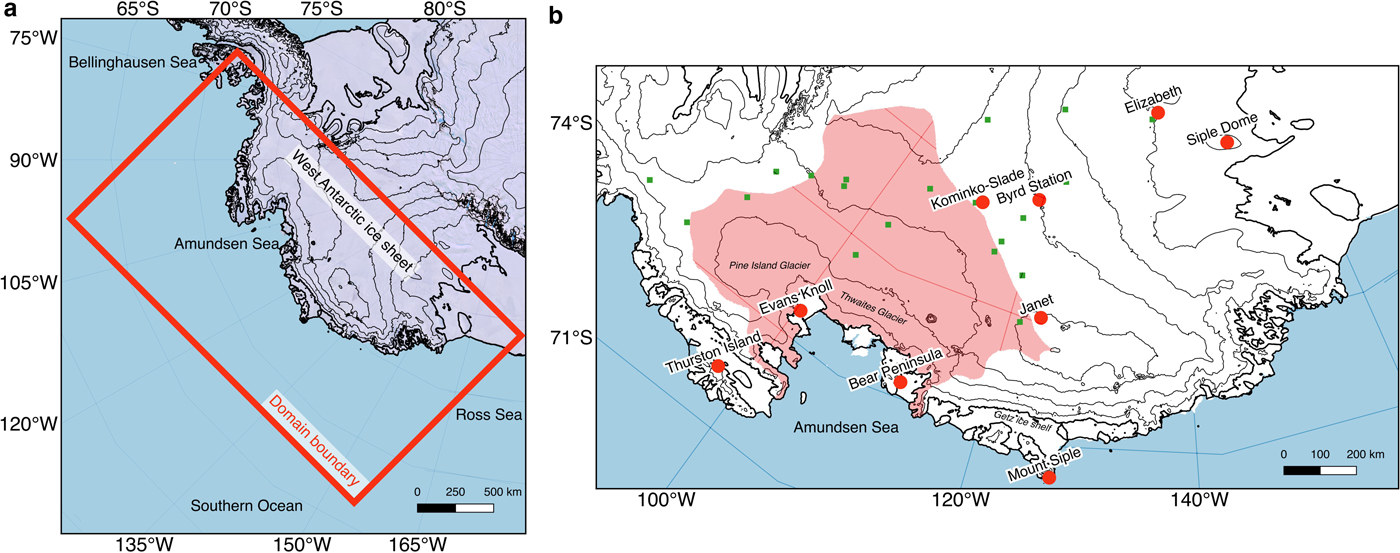
Overview of the model domain. (a) Location of the domain on the Antarctic ice sheet and neighbouring ocean areas. The red square shows the domain boundary. (b) Zoom on inner model domain with the locations of the automatic weather stations (AWSs) shown with red dots. The red shading shows the area for which the mass balance is calculated (see Fig. 11). The green squares show the locations of the PAGES 2k firn cores (see Fig. 9). In both maps (and in all maps that follow), the thick black line is the ice-sheet grounding line (from Depoorter and others, Reference Depoorter2013) and the thin black lines show elevation (Bamber and others, Reference Bamber, Gomez-Dans and Griggs2009) at 500 m contour intervals.
The intense ice/ocean interactions are strongly regulated by atmospheric variability, which is larger in the ASE than anywhere on the Earth (Connolley, Reference Connolley1997). The atmospheric conditions over the ASE are primarily determined by the strength and location of the Amundsen Sea Low (ASL, Raphael and others, Reference Raphael2015), the climatological low-pressure centre located north of the ASE. In turn, the atmospheric dynamics are in part driven by tropical climate variability (Bromwich and others, Reference Bromwich, Monaghan and Guo2004; Bertler and others, Reference Bertler, Naish, Mayewski and Barrett2006; Ding and others, Reference Ding, Steig, Battisti and Kuttel2011; Steig and others, Reference Steig, Ding, Battisti and Jenkins2012; Clem and Renwick, Reference Clem and Renwick2015) as well as atmospheric pressure differences between low and high latitudes of the Southern Hemisphere (i.e. the Southern Annual Mode SAM, Scambos and others, Reference Scambos2017). The position and strength of the ASL not only determine the meridional flow that control CDW delivery onto the continental shelf (Thoma and others, Reference Thoma, Jenkins, Holland and Jacobs2008), but also drives atmospheric heat and moisture supply to the ice sheet (Nicolas and Bromwich, Reference Nicolas and Bromwich2011; Fyke and others, Reference Fyke, Lenaerts and Wang2017). Coastal ASE receives some of the highest snowfall amounts of Antarctica (Lenaerts and others, Reference Lenaerts, van den Broeke, van de Berg, Van Meijgaard and Kuipers Munneke2012b), owing to frequent landfall of deep moisture plumes originating from the tropics, so-called atmospheric rivers (Gorodetskaya and others, Reference Gorodetskaya2014).
These atmospheric rivers interact with the complex topography, generating steep precipitation gradients (Nicolas and Bromwich, Reference Nicolas and Bromwich2011). Behind these coastal ridges, moisture quickly dissipates, leaving the interior ice sheet much drier. In order to resolve these gradients, atmospheric climate models should resolve features smaller than the typical length scale of topography, i.e. 10–100 km, which is smaller than the resolution currently employed in global climate models. Even though some models simulate large-scale atmospheric patterns correctly, their resulting precipitation patterns are smoothed out because topography is poorly resolved (Medley and others, Reference Medley2013). As a result, most climate models overestimate interior precipitation over Antarctica (Palerme and others, Reference Palerme2016). To overcome these deficiencies, regional atmospheric climate models are useful tools (Lenaerts and others, Reference Lenaerts, van den Broeke, van de Berg, Van Meijgaard and Kuipers Munneke2012b; Van Wessem and others, Reference Van Wessem2014b). They dynamically downscale the large-scale atmospheric structure to horizontal resolutions that are more consistent with the ice sheet topography, and their resulting climate gradients are better suited to drive ice sheet and ocean models.
Additionally, an important mechanism to drive ice-shelf hydrofracturing and ice cliff instability is ice-shelf surface melting (DeConto and Pollard, Reference DeConto and Pollard2016). The ratio between surface melt and snowfall is an indicator of ice-shelf firn ‘health’ (Kuipers Munneke and others, Reference Kuipers Munneke, Ligtenberg, Van Den Broeke and Vaughan2014): as surface melt increases under constant snowfall, firn saturates with water and warms, decreasing pore space and enhancing risk for meltwater ponding, and surface-based water can percolate all the way to the bottom of the ice shelf. Potentially, this results in catastrophic ice-shelf breakup, which was evidenced by the Larsen B breakup in early 2002. Although mapping surface melt extent is possible with remote sensing (e.g. Tedesco and Monaghan, Reference Tedesco and Monaghan2009), deriving surface melt volume is much more challenging (Trusel and others, Reference Trusel, Frey, Das, Munneke and Van Den Broeke2013), as it requires in situ melt observations that are not always representative for a larger area. Moreover, surface melt rates are highly spatially heterogeneous over ice shelves and the ice sheet. Melt is typically concentrated in a narrow band close to the ice-shelf grounding line (Luckman and others, Reference Luckman2014; Hubbard and others, Reference Hubbard2016), where warm winds erode the firn and create a local microclimate (Lenaerts and others, Reference Lenaerts2017b). Melt events, even those that are marginal and short-lived, can substantially alter the energy balance during the rest of the melt season (Trusel and others, Reference Trusel, Frey, Das, Munneke and Van Den Broeke2013). Regional climate models, which incorporate the necessary surface processes, provided they are employed at fine resolution, have been shown to successfully represent these features (Lenaerts and others, Reference Lenaerts, van den Broeke, van Angelen, van Meijgaard and Déry2012a, Reference Lenaerts2014a; Van Wessem and others, Reference Van Wessem2016; Lenaerts and others, Reference Lenaerts, Van Tricht, Lhermitte and L'Ecuyer2017a).
To resolve these important climate and surface mass balance (SMB) processes over the ASE, we employ the regional atmospheric climate model RACMO2 at unprecedentedly high horizontal resolution (5.5 km) over this region for the period 1979–2015. Here we present the results of this simulation, evaluate the results using novel observational data, and discuss the added value of the high horizontal resolution. Section ‘Methods and data’ presents the numerical setup and observational data, section ‘Results’ discusses the results, and section ‘Discussion and conclusions’ gives conclusions and discussion.
METHODS AND DATA
Regional climate model
In this study, we use the Regional Atmospheric Climate MOdel, version 2.3p2 (Noël and others (Reference Noël2017), RACMO2 hereafter). RACMO2 combines the representation of atmospheric dynamics of the High Resolution Limited Area Model (HIRLAM, version 5.0.6 Unden and others, Reference Unden2002), while the description of the physical processes is adopted from the European Centre for Medium-range Weather Forecasts (ECMWF) Integrated Forecast System (IFS) (ECMWF-IFS, 2008). It has been adapted for use over the large ice sheets of Greenland and Antarctica, including a multi-layer snow model to calculate melt processes (Ettema and others, Reference Ettema, van den Broeke, van Meijgaard and van de Berg2010), surface albedo (Kuipers Munneke and others, Reference Kuipers Munneke2011), and blowing snow (Lenaerts and Van Den Broeke, Reference Lenaerts and Van Den Broeke2012). RACMO2 topography is based on the Bamber and others (Reference Bamber, Gomez-Dans and Griggs2009) digital elevation model, derived from a combination of satellite radar and laser data.
Previous studies using RACMO2 found that the model underestimates the amount of clouds and the resulting snowfall in the ice-sheet interior of both Greenland (Noël and others, Reference Noël2015) and Antarctica (Van Wessem and others, Reference Van Wessem2014a). Therefore, in this updated version, the critical cloud content for efficient precipitation generation has been increased by a factor 2 and 5 for liquid/mixed and ice clouds, respectively. As a result, cloud content can now be advected further inland, likely further decreasing biases in the AIS interior (Van Wessem and others, Reference Van Wessem2014a). Furthermore, the linear saltation snow load parameter (Eqn (24), Déry and Yau, Reference Déry and Yau1999) used in the RACMO2 drifting snow is halved, i.e. from 0.385 to 0.190 (Lenaerts and others, Reference Lenaerts2014b), effectively halving the horizontal drifting snow transport and drifting snow sublimation flux, without changing the length nor frequency of the drifting snow events.
In this setup, the climate model is employed for a spatial domain encompassing a large part of the WAIS coastal region (Fig. 1), stretching from the Wilkins ice shelf in the east (at ~75°W) to the central Ross ice shelf in the west (~175°W). A large part of the domain contains ocean/sea-ice covered points, to ensure that the northern edge of the domain, which receives a large part of the large-scale atmospheric fluxes transported into the domain, is located sufficiently far away (>1000 km) from the ice-sheet coast. Moreover, this allows using these atmospheric data as forcing for regional ASE ocean models. RACMO2 is forced at these edges by vertical atmospheric profiles of temperature, humidity and winds, as well as sea surface temperature and sea-ice cover, from ERA-Interim atmospheric reanalysis (Dee and others, Reference Dee2011), which is available from January 1979 onwards. The choice of ERA-Interim forcing is justified by its realistic climate over the high-latitude Southern Hemisphere, outperforming other reanalysis products in its representation of near-surface climate over Antarctica as a whole (Bracegirdle and Marshall, Reference Bracegirdle and Marshall2012) and the Amundsen Sea region (Jones and others, Reference Jones2016). The forcing from ERA-Interim at the ocean surface implies that our modelling approach does not simulate ocean dynamics and their impact on ice-shelf dynamics. In RACMO2, the ice shelves are assumed to be grounded ice and are not allowed to change thickness or shape. RACMO2 is employed at a horizontal resolution of 5.5 km, resulting in a domain of 456 longitudinal and 361 latitudinal grid cells. Here we present the RACMO2 results for the time period January 1979–December 2015. We compare the RACMO2 data with new observations of near-surface climate, surface melting, and SMB, and with RACMO2 output generated at a lower horizontal resolution (27 km, van Wessem and others, Reference Van Wessem2017). The latter is produced from a RACMO2 simulation performed for the full Antarctic domain, with exactly the same physics as the high-resolution simulation. This allows us to assess the added value of the higher resolution in representing the coastal WAIS climate and SMB.
Observations
Weather stations
To evaluate the performance of the high-resolution RACMO2 simulation, the simulated climate was compared to 2-m temperature (T2m) and 10-m wind speed (FF10m) observations from nine AWSs located in West Antarctica (Fig. 1, Table 1). AWS data at three-hourly intervals were obtained from Antarctic Meteorological Research Center (AMRC) and AWS program (https://amrc.ssec.wisc.edu/).
Overview of weather stations used in the comparison with RACMO2

The two rightmost columns show the number of months with data availability and the total number of months (available/total).
The nine stations are relatively evenly distributed over the domain (Fig. 1b) and can be classified into coastal stations (from east to west: Thurston Isl., Evans Knoll, Bear Pen. and Mt. Siple) and interior stations. Of these latter stations, three are located close to the West Antarctic ice divide (Byrd Station, Kominko-Slade and Janet) and two are on the south side of the divide, near the Siple Coast (Elizabeth, Siple Dome). For all locations, the grid points closest to the weather station were used for the comparison (Table 1), with a single exception: for Bear Peninsula, a R5.5 neighbouring grid point was chosen to better mimic the conditions of the location of the AWS, situated on a rock outcrop on the edge of the peninsula and situated ~200 m above the ice shelf. For the coastal stations, the elevation difference between the AWS location and RACMO grid points is often significant (50–100 m, Table 1), since the AWS is usually situated on bedrock outcrops or nunataks in rough topographical terrain.
Almost all stations have data available for the last 5 years (2011–15), with only three stations having records that extend back before 2008: Byrd Station from 1980 onwards, Elizabeth from 1996 onwards and Mount Siple from 1992 onwards (Table 1). Monthly averages are calculated from the 3-hourly AWS data and a monthly average was used in the evaluation if data were available for at least 95% of time during that month. For the evaluation of 3-hourly data, all available AWS data were used.
Radar and firn cores
SMB can be observed using a combination of radar (airborne or ground-based) and firn cores. The reconstruction relies on internal reflections in firn and ice caused by density variations due to surface conditions at the time of deposition, which can therefore be assumed to be of isochronous origin (Vaughan and others, Reference Vaughan, Corr, Doake and Waddington1999). The respective signal travel times measured by the radar can be converted into water equivalent depth using an empirical relation between firn density and the dielectric constant (Kovacs and others, Reference Kovacs, Gow and Morey1995), with a regionally averaged firn density profile based on density measurements at distinct firn core locations.
Here we use two datasets that combine radar and firn cores. Firstly, the airborne shallow radar suite developed by the Center for Remote Sensing of Ice Sheets (CReSIS) and flown on NASA's Operation IceBridge (OIB) mission provides an unparalleled peek into the subsurface firn stratigraphy. We specifically use the snow radar, which is an ultra-wideband microwave radar system that operated over the frequency range of 4–6 GHz in 2009 and 2–6.5 GHz subsequently (Leuschen, Reference Leuschen2014). This frequency-modulated continuous-wave (FM-CW) radar system images the stratigraphy in the upper 20–30 m of the ice sheet with fine vertical resolution (a few centimetres) and an along-track spacing of a few tens of metres (Medley and others, Reference Medley2013; Panzer and others, Reference Panzer2013). Snow radar data have been collected in Antarctica annually since 2009 (with the exception of 2015), covering much of coastal West Antarctica and its peripheral ice shelves. The use of OIB airborne radar allows us to evaluate the spatial pattern of SMB over the complex topography surrounding the Getz Ice Shelf, which includes several prominent ice domes. We use data collected on 5 November 2010, which surveys several of these ice domes. Although Medley and others (Reference Medley2013) mapped several annual horizons for evaluation of temporal variations in SMB, because we are mainly interested in evaluating the spatial patterns in R5.5, we map a single, strong horizon in the radar data that corresponds to 3 years of accumulation (2008–10). After picking the surface return, we applied an automated picker to find several strong peaks in return power below the surface for each trace, but recorded only the third peak (i.e. 3 years of accumulation). Erroneous picks were filtered out, and visual inspection of the horizon pick confirmed we were consistently picking the same horizon. We use a method described in Medley and others (Reference Medley2015), which allows for spatial variations in the firn density profile in both radar-depth estimation as well as conversion to water equivalence. The method iteratively solves for a depth-density profile at each measurement that is consistent with the radar-derived accumulation rate as well as long-term modeled 2-m air temperature from MERRA-2 and an initial density of 350 kg m−3. Thus, we create 3-year mean annual estimates of 2008–10 SMB. To improve the comparison with RACMO2, we use OIB Airborne Topographic Mapper resampled and smoothed nadir elevation measurements (ILATM2; Krabill, Reference Krabill2010). We additionally use 1985–2009 mean annual radar-derived accumulation presented by Medley and others (Reference Medley2014) to evaluate RACMO2 over Pine Island and Thwaites catchments. The ~20 000 measurements are spaced at ~500 m increments over resulting in 10 000 km of along-track data covering an area of 300 × 103 m2.
Secondly, we use new firn core and ground-penetrating radar (GPR) records collected within the scope of NERC's Ice Sheet Stability Programme iSTAR. These were acquired on Pine Island Glacier for reconstructing SMB along a 900-km long traverse covering the glacier's main tributaries. The radar acquisition was carried out in the 2013/14 field season using a commercially available pulseEKKO PRO device operating at 100 MHz with transmitter and receiver antennae in common-offset mode. The radar data were routinely processed by a static correction, bandpass filtering, background removal, and gain correction. A distinct reflector was picked by eye along most of the traverse. Where the radar data were interrupted along the traverse, the age-depth distribution of the firn cores (see below) served as a guidance to identify the corresponding reflector. Firn cores of ~50 m depth each were drilled in the 2014/15 field season at ten main landmarks of the traverse. Their chronologies were established by analysing annual cycles in hydrogen peroxide (Sigg and Neftel, Reference Sigg and Neftel1988), by which the picked reflector was dated to stem from ~1986. The SMB was then computed by dividing water equivalent depth of the reflector by its age. The uncertainty of the SMB incorporates the wavelength of the radar wavelet (Navarro and Eisen, Reference Navarro, Eisen, Pellikka and Rees2009), the uncertainty in speed of light as reflected in the variability of density in the ensemble of firn cores, the variance of the ages at the core locations, and an additional age uncertainty of 1 year to accommodate the delay between radar and firn core acquisition.
In complement to these two datasets, we use a recently compiled dataset of firn core SMB for RACMO2 model evaluation. Coordinated by the Past Global Changes (PAGES) Antarctica 2k working group, all available firn core SMB records on Antarctica were collected and thoroughly quality checked (Thomas and others, Reference Thomas2017). Here we use the 21 cores for the period 1979–2012 (or the temporal subset of this period covered by the firn core) spread around the R5.5 domain (Fig. 1b, Thomas and others, Reference Thomas2017). All of these cores were drilled at elevations between 1000 and 2000 m above sea level, with a mean SMB varying from 100 to 500 mm w.e. a−1.
Remote sensing of surface melt
RACMO2 surface melt volume is compared to the 2000–09 mean surface melt volume derived from QuikScat scatterometery available at ~5 km horizontal resolution (Trusel and others, Reference Trusel, Frey and Das2012). Because this dataset encompasses only 10 years, and interannual variability in surface melt is substantial (Kuipers Munneke and others, Reference Kuipers Munneke, Van Den Broeke, King, Gray and Reijmer2012), temporal variations of surface melt in RACMO2 are compared with a new surface melt occurrence dataset spanning the entire simulation period 1979–2015 (Nicolas and others, Reference Nicolas2017). This dataset uses brightness temperatures (Tbs) from a series of spaceborne sensors: The Scanning Microwave Multichannel Radiometer (SMMR) onboard the Nimbus-7 satellite (1978–87); the Special Sensor Microwave/Imager (SSM/I) onboard successive satellites (F-8, F-11 and F-13) from the Defense Meteorological Satellite Program (DMSP; 1987–2009); and the Special Sensor Microwave Imager Sounder (SSMIS) onboard DMSP F-17 satellite (2006-present). The data are provided by the National Snow and Ice Data Center on an equal-area scalable Earth grid with a nominal resolution of 25 km (Armstrong and others, Reference Armstrong, Knowles, Brodzik and Hardman1994; Knowles and others, Reference Knowles, Njoku, Armstrong and Brodzik2000). We use horizontally polarized Tb data in the K-band (18 GHz for SMMR, 19 GHz for SSM/I-SSMIS), previously used for melt detection over ice sheets (e.g. Liu and others, Reference Liu, Wang and Jezek2006; Picard and others, Reference Picard, Fily and Gallee2007; Tedesco, Reference Tedesco2009). These observations are available twice-daily (from the ascending and descending satellite overpasses). More details on the melt detection algorithm are described by Nicolas and others (Reference Nicolas2017). For a given grid cell and a given day, we determine that melt was occurring as soon as one of the two daily Tb observations exceeded a threshold value (Tbmelt) defined as Tbmelt = Tbref + δT, where δT = 30 K and Tbref is a reference temperature. Tbref is calculated as the 12-month average from 1 April to 31 March after filtering out all melt days as in Torinesi and others (Reference Torinesi, Fily and Genthon2003). To compare model and observations, we use the melting index (Zwally and Fiegles, Reference Zwally and Fiegles1994), which is defined as the annual accumulated product (1 April–31 March) of daily melt occurrence (units in km2 × days). For the model, we use a predefined melt threshold of 3 mm/day, to optimize the correspondence with the observations.
RESULTS
Near-surface temperature and wind
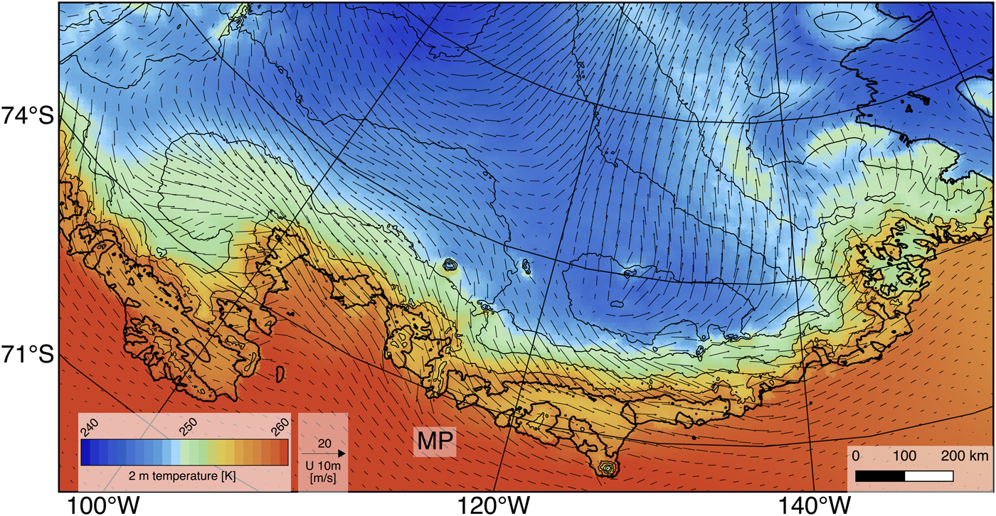
Simulated near-surface temperature and wind speed fields display a high level of spatial detail (Fig. 2). The annual mean temperature is highest (>260 K) over the oceans adjacent to the ice sheet. Generally, near-surface temperatures gradually decrease from the lower to the high-elevation areas, but the high-resolution model displays some interesting regional climate phenomena. For instance, the temperatures are higher in the grounding zone (0–50 km seaward from the grounding line), along the high-sloping areas inward of the ice shelves, and on the sides of the small ice domes and ice rises, than on the ice shelves themselves. This is explained by the enhanced turbulent mixing in these areas (King, Reference King1998; Lenaerts and others, Reference Lenaerts2017b). The ice shelves themselves are typically cold, especially the Ross Ice Shelf, where surface-based temperature inversions are known to be well developed and associated with low-level jets (Seefeldt and Cassano, Reference Seefeldt and Cassano2008). The general wind field is largely dominated by katabatic flow originating from the interior ice sheet (Fig. 2). The strongest mean winds are found over confluent topography such as the interior Pine Island Glacier (76°S, 95°W). Additional, smaller-scale wind patterns are discernible over some coastal ice domes, which act to accelerate winds. One of the clearest examples is Martin Peninsula (74°S, 115°W, MP in Fig. 2), where mean wind speeds vary from 5 m s−1 on the lee side to 9 m s−1 on its north side (not shown). This local flow acceleration due to larger-scale topography shows remarkable similarities to, but is much more poorly documented than, the southern Greenland ‘tip jet’ (Doyle and Shapiro, Reference Doyle and Shapiro1999; Moore and Renfrew, Reference Moore and Renfrew2005).
Annual mean (1979–2015) simulated (R5.5) near-surface temperature (at 2 m, colours) and wind vectors (at 10 m, arrows). The location of Martin Peninsula is marked by MP.
The evaluation of the simulated T2m and FF10m for both RACMO2 simulations are shown in Figures 3, 4, and the statistics per station are listed in Tables A1, A2 (in the appendix), respectively. For the monthly average near-surface temperature of all stations (Fig. 3a), little difference can be discerned between the high- and low-resolution RACMO2 results; mostly, simulated temperatures are within 2 K of the observed temperatures, although some outliers are found with a maximum absolute bias of 5 K. Also, the points are centered on the 1:1-line, indicating that there is no clear bias in either simulation. The variance and the RMSE show that R5.5 (0.97 and 3.83) slightly outperforms R27 (0.95 and 4.78), with the same being true for almost all individual stations (Table A1). The 3-hourly data for all stations are not plotted in Figure 3a due to the high number of measurements, but they show the same pattern. The difference between the R5.5 and R27 is slightly larger for the 3-hourly than for the monthly data, with R5.5 again scoring better.
Scatter plots of observed (AWS) vs. simulated (R5.5 in green, R27 in blue) near-surface temperature. (a) All stations; (b) Bear Peninsula; (c) Byrd Station. In panels (b) and (c), the opaque markers show the 3-hourly data, and the clear markers show the monthly mean data. The statistics are given for both monthly and 3-hourly comparisons in each plot. The coloured lines show the 1:1 line (black) and the best linear fit for R5.5 (green) and R27 (blue).

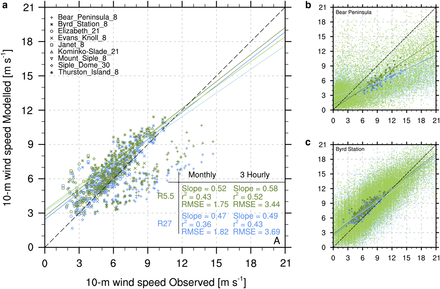
Scatter plots of observed (AWS) vs. simulated (R5.5 in green, R27 in blue) near-surface wind speed. (a) All stations; (b) Bear Peninsula; (c) Byrd Station. In panels (b) and (c), the opaque markers show the 3-hourly data, and the clear markers show the monthly mean data. The statistics are given for both monthly and 3-hourly comparisons in each plot. The coloured lines show the 1:1 line (black) and the best linear fit for R5.5 (green) and R27 (blue).
Figures 3b, c show the same comparison only for two individual stations and including the 3-hourly observations. For the inland station (Byrd station, Fig. 3c) the pattern is similar to the one for all stations combined: no bias from the 1:1-line and no visual differences between R5.5 and R27, while the statistics slightly favour R5.5 over R27 (Table A1). For the coastal station (Bear Peninsula, Fig. 3b) the R27 simulation shows a clear negative temperature bias compared with the observations, which is probably caused by the lack of topographical detail in R27. In the low-resolution simulation, the topography is smoothened and the grid point is located on the flat Dotson Ice Shelf where the strong near-surface inversion causes very cold winter conditions. In reality, however, the AWS is situated on a rock outcrop ~200 m above the ice shelf where it is less impacted by these cold winter inversion conditions. In R5.5, the topographical difference between the flat ice shelf and surrounding islands is much better captured leading to a better representation of the near-surface temperature.
For the 10-m wind speed comparison roughly the same conclusion can be drawn from the 2-m temperature comparison: on average, R5.5 slightly outperforms R27 on both the monthly and 3-hourly data (Fig. 4a and Table A2). However, the agreement between observations and modelled wind speed is significantly worse than for temperature. For Bear Peninsula (see also Fig. 3b) and Thurston Island, the wind speed is underestimated by ~40% by both model simulations. Again, this difference is likely caused by the position of the AWS on topographical highs resulting in high measured wind speeds. Interestingly enough, this does not apply to Evans Knoll, although the station is also located at the top of an island in a large flat ice shelf.
For the inland stations, the agreement is much better with lower RMSE values and slopes near 1.0 (Table A2). However, a systematic bias is observed with simulated wind speeds slightly higher than those measured. This is especially clear for Byrd Station (Fig. 4c) where the monthly mean RACMO2 values show an overestimation of observed wind speed of 1.0–1.5 m s−1, while the slope is virtually 1.0. As the overestimation is present in both model simulations, a possible cause could be that the roughness length in RACMO2 is slightly too low, yielding too strong near-surface winds. Other possible explanations are related to the excessive momentum diffusion in RACMO2, and/or the limited vertical resolution (only three vertical layers below 100 m), which limits the ability of a regional climate model to represent the boundary layer near the coastal domes.
Noteworthy is the cluster of points at the bottom left of Figure 4a that shows low measured wind speeds in combination with high simulated wind speeds. These respective months are probably affected by rime formation on the wind meter, as some 3-hour data show near-zero wind speed conditions, while RACMO2 simulates >10 m s−1. Especially the statistics of Janet station (Table A2) might be affected by this as this occurs in 10–15% of the measured months. We decided not to remove any 3-hourly or monthly data as we had no data to determine whether a measurement was a normal outlier or was the result of instrument malfunctioning by e.g. rime formation.
Surface melt
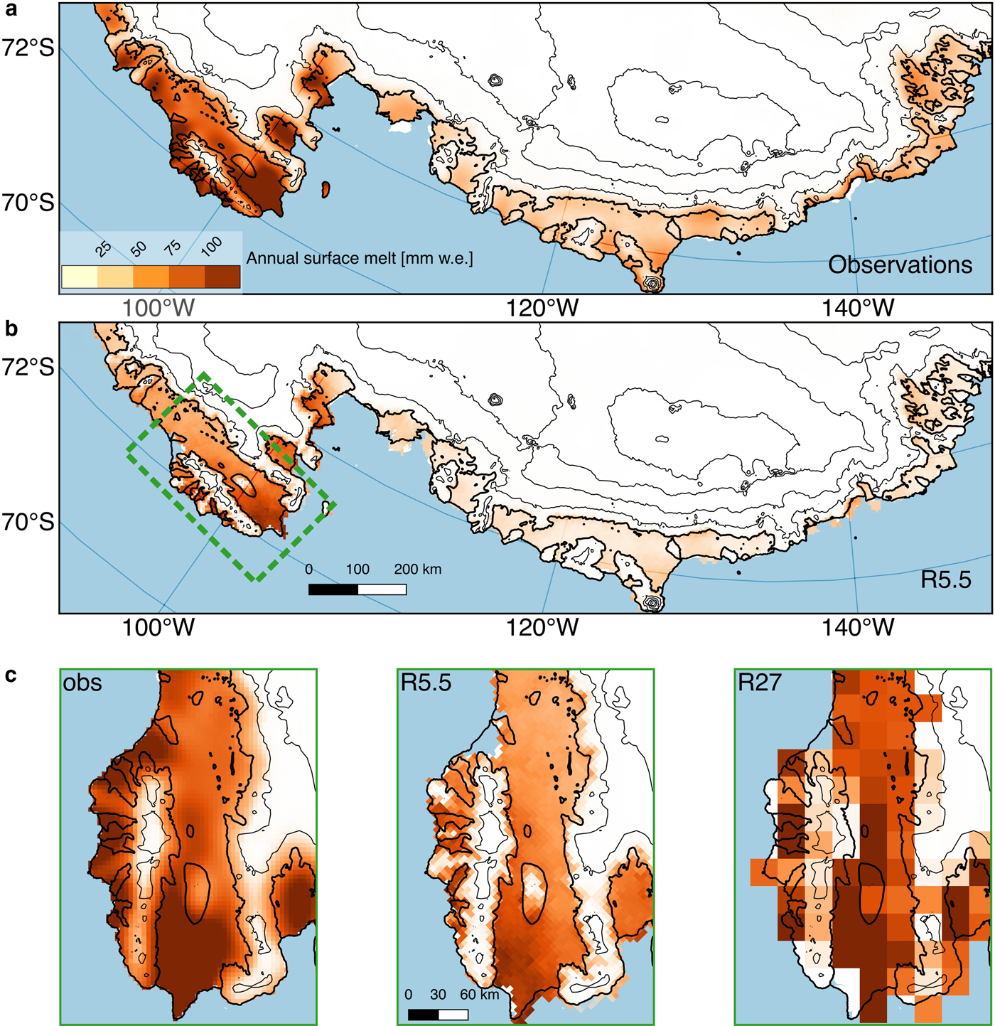
With the cold climate characterizing much of WAIS, surface melt does not frequently occur over most of the grounded ice sheet (Fig. 5), and is confined to ice shelves. The highest surface melt rates (>100 mm w.e. a−1) are found over parts of Abbott ice shelf, Cosgrove ice shelf and eastern Pine Island ice shelf. Note that these melt rates are still a factor of five to ten lower than those observed on the eastern Antarctic Peninsula ice shelves (Trusel and others, Reference Trusel, Frey, Das, Munneke and Van Den Broeke2013). Much lower surface melt rates prevail over the ice shelves in the western half of the domain, and surface melt on Ross Ice Shelf (not shown) only occurs in anomalously warm summers, as driven for example by strong El Niño conditions (Nicolas and others, Reference Nicolas2017). Although the absolute surface melt rates are 30–50% lower, the patterns of RACMO2 surface melt agree very well with the observations. One possible reason for the underestimation of surface melt, apart from the uncertainty associated with the conversion from radar backscatter to surface melt volume in the QSCAT observational product, is the positive RACMO2 summer albedo bias (Lenaerts and others, Reference Lenaerts2017b), which delays the onset of the melt-albedo feedback (Van den Broeke and others, Reference Van den Broeke, König-Langlo, Picard, Kuipers Munneke and Lenaerts2010). Another explanation is related to the horizontal resolution of the model: although the R27 model does not resolve the spatial melt gradients over Abbott ice shelf (Fig. 5) that are observed and simulated in R5.5, it shows higher surface melt rates that are more consistent with the observations. This suggests that RACMO2, when employed at higher resolution that better resolves local topography, generates too cold conditions on the ice shelf through overestimating ice-shelf snowfall (mitigating the melt-albedo feedback) and/or reinforcing the temperature inversion by under-representing turbulent mixing.
Annual mean 2000–09 surface melt volume (mm w.e. a−1) according to (a) observations derived from QuikScat and (b) R5.5. Panel (c) shows a comparison of observations, R5.5 and R27 on the Abbott ice shelf.
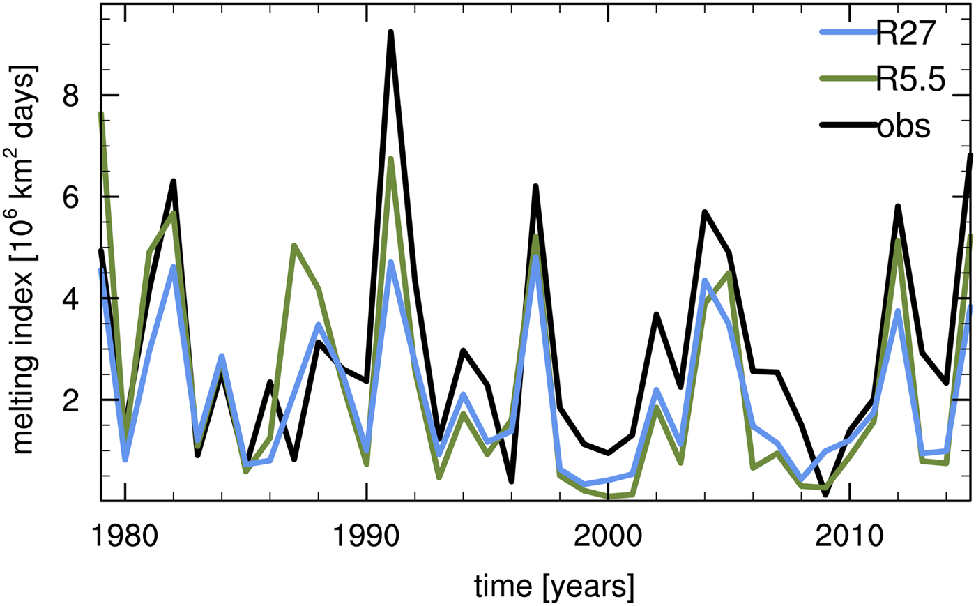
Interannual variability of area-integrated surface melt occurrence is compared with observations in Figure 6. Because we optimized the surface melt threshold in RACMO2, the model estimates (2.3 ± 2.1 106 km2 × days in R5.5 and 2.0 ± 1.4 106 km2 × days in R27) agree very well with the observations (2.9 ± 2.1 106 km2 × days), with all datasets displaying similarly large interannual variability (R 2 = 0.64 between R5.5 and the observations, and R 2 = 0.76 between R27 and the observations). Peak melt years, such as 1991, are well simulated by RACMO2. This signals that the model is able to simulate the atmospheric drivers and atmosphere-snow feedbacks causing variability in melt. Additionally, it shows that the enhanced horizontal resolution in R5.5 does not improve the interannual variability of simulated surface melt. One possible reason is that, unlike R27, R5.5 does not include ERA-Interim upper-air relaxation (Van de Berg and Medley, Reference Van de Berg and Medley2016), which improves temporal variability of SMB in RACMO2.
Time series (1979–2015) of annual melt index for the area between 100 and 160°W according to observations (black) and R5.5. To define the occurrence of surface melt in R5.5, we use a daily surface melt threshold of 3 mm w.e. Note that each year (e.g. 1979) refers to the summer starting in that year (e.g. 1979–80).
Surface mass balance
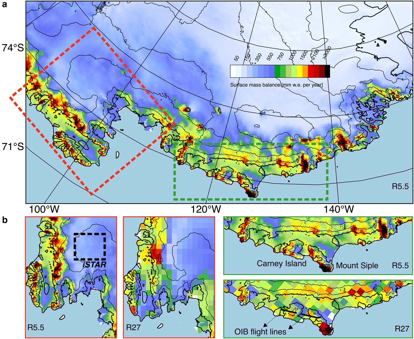
The simulated SMB field is illustrated by Figure 7a. Very high SMB (>1000 mm w.e. a−1), dominated by snowfall, is found along many coastal ice sheet slopes, especially those that are aligned orthogonal (i.e. west to east) to the prevalent atmospheric moisture flux direction (i.e. north to south). Coastal areas in the lee of other topography, such as Pine Island glacier (100°W, 75°D) receive much less precipitation. The Ross Ice Shelf, sheltered from much of the synoptic activity in the Amundsen region, is comparably very dry (<200 mm w.e. a−1). SMB quickly decreases with elevation on the grounded ice sheet, but the SMB remains higher in the western regions, where ice-sheet surface slopes are negative, than towards the east, where slopes remain positive far inland. This is especially evident over the ASE (east of 120°W) , where SMB exceeds 500 mm w.e. a−1 up to 2000 m a.s.l.
Annual mean (1979–2015) simulated (R5.5) SMB. (a) Entire domain; (b) Zooms on Abbott ice shelf and Getz ice shelf areas (see red and green squares in (a)), including comparisons with R27. The approximate locations of the iSTAR study area and OIB flight lines are shown in (b).
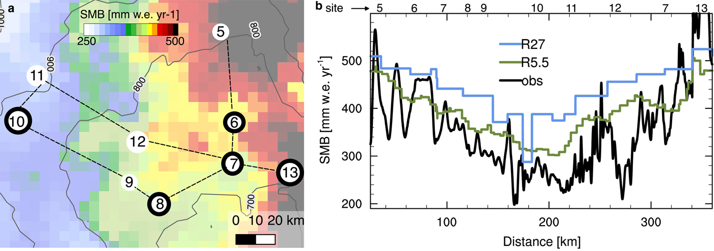
Over Pine Island and Thwaites glacier catchments, the spatial correspondence of R27 and R5.5 with 1985–2009 mean annual radar-derived SMB (Medley and others, Reference Medley2013, Reference Medley2014, not shown) shows a similarly good agreement with observations for both datasets (R 2 = 0.69 for R5.5, R 2 = 0.67 for R27). The dry bias relative to the radar observations (mean SMB = 409 mm w.e. a−1) is enhanced in R5.5 (mean = 355 mm w.e. a−1) as compared with R27 (mean = 372 mm w.e. a−1), but remains consistent with other atmospheric reanalysis datasets (Medley and others, Reference Medley2013). To complement this analysis, we use firn core and GPR observations obtained in this area by the iSTAR project (see Fig. 7b). These allow us to perform a comparison of R5.5 and R27 (Fig. 8). Along the iSTAR transect, the observed SMB decreases from 450 mm w.e. a−1 to 250 mm w.e. a−1 in the first part of the transect (from sites 5 to a) that runs from southeast to northwest, and increases back to >500 mm w.e. a−1 when returning to the west (sites 11 to 13). Although R5.5 and R27 both broadly represent that pattern, R5.5 approaches the observations much better than R27. The mean bias with respect to the observations along the transect is reduced from 84 mm w.e. a−1 in R27 to 32 mm w.e. a−1 in R5.5. The RMSE decreases from 110 mm w.e. a−1 in R27 to 77 mm w.e. a−1 in R5.5. Moreover, R5.5 partly reproduces smaller-scale variations that are present in the observations, such as the strong SMB increase around sites 11 and 12. This indicates that R5.5 better reproduces the absolute SMB, as well as its gradients, on Pine Island Glacier.
Comparison of observed and simulated (R5.5 in green, R27 in blue) SMB along iSTAR transect (see Fig. 7b for location). (a) location of firn cores (encircled white dots), other iSTAR landmarks (open white dots), and GPR transect (dashed lines), with R5.5 mean SMB and 100 m elevation contours in the background; (b) 1980–2014 mean SMB along transect. The location of the sites is shown on the top.
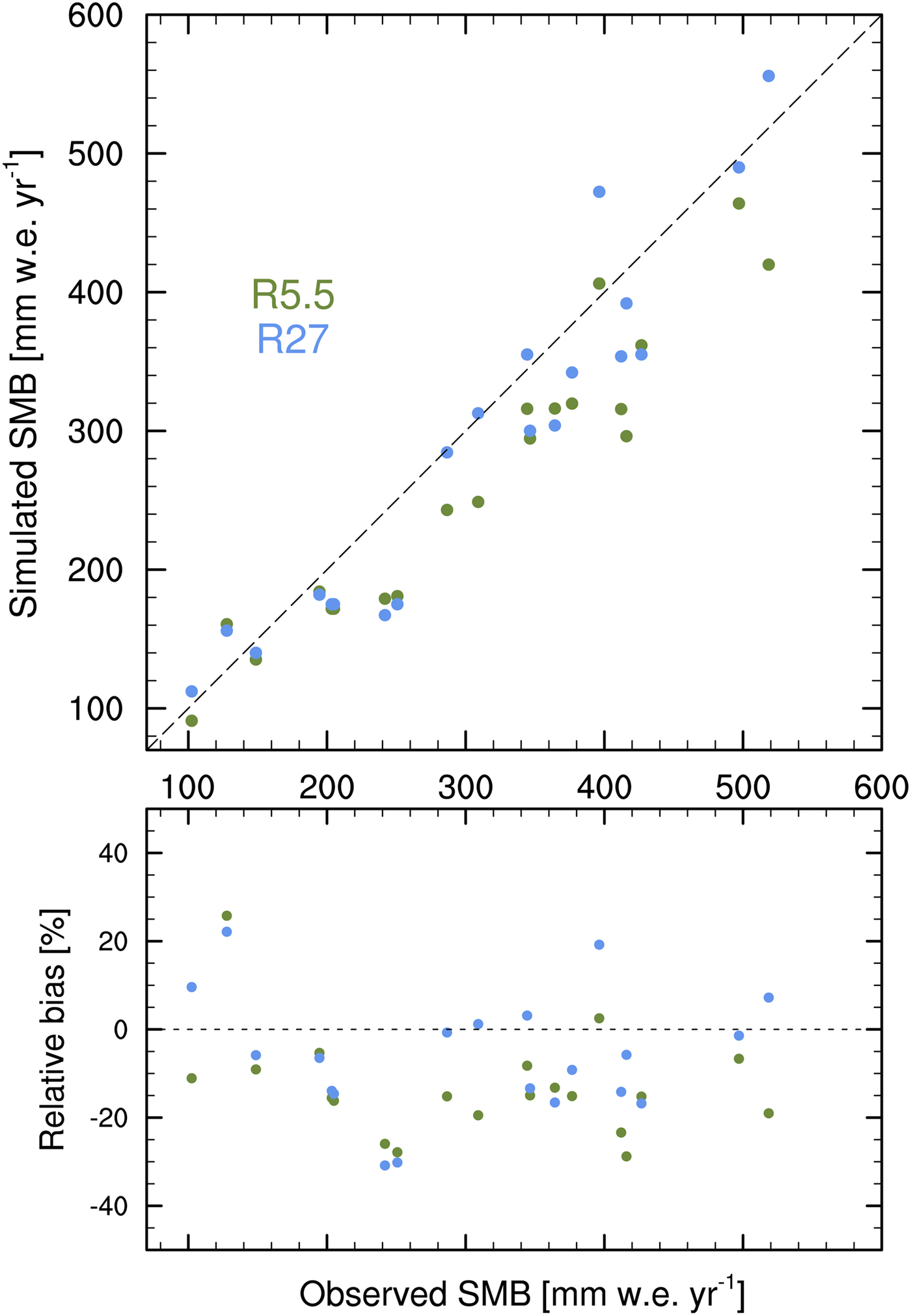
Next, RACMO2 is compared to available PAGES 2k ice cores (Fig. 9) for the overlapping period. Overall, both R5.5 and R27 compare very well to the available SMB observations, with a relative bias not exceeding 30% for all firn cores. In contrast to the better performance of R5.5 with respect to the iSTAR results, we find here a slightly better overall performance of R27 (mean bias =<1 mm w.e. a−1) than of R5.5 (mean bias =−17 mm w.e. a−1). The SMB underestimation in R5.5 is most strongly manifested at the firn core locations in the eastern part of our domain (around 90°W, not shown). We speculate that R5.5, at this high horizontal resolution, simulates excessive orographic snowfall on the coastal slopes in this region (Fig. 7), leaving the interior areas with a dry bias.
Scatter plot of observed (firn cores) vs. simulated (R5.5 in green, R27 in blue) annual mean (1979–2012, or the overlapping sub-period) SMB. (a) absolute values; (b) relative bias of the models with respect to the observations.
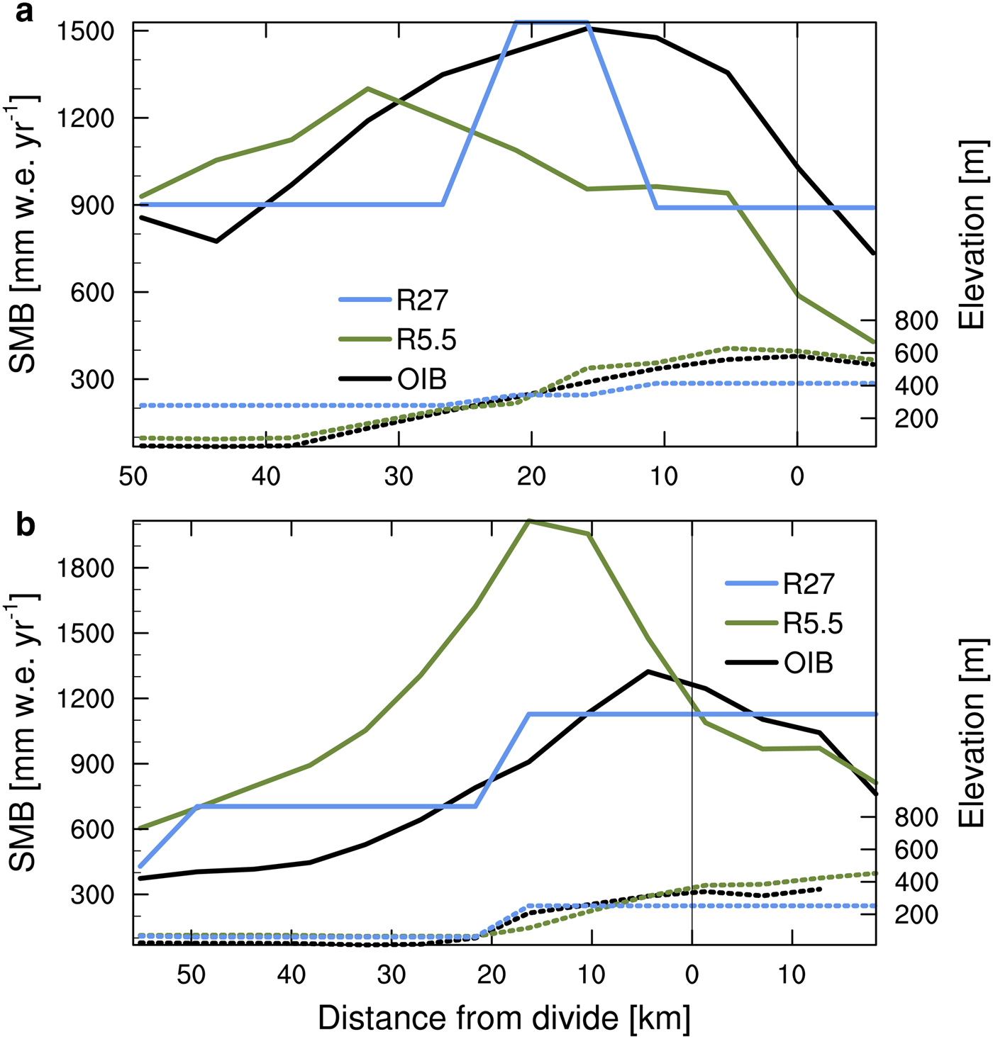
In the coastal regions, where no firn records are available, the high resolution enables R5.5 to represent the large SMB gradients induced by topography that has finer horizontal scales (<50 km), and are thus not resolved by global atmospheric reanalyses or coarser-scale models, such as R27. This is evidenced by the much smoother gradients in R27 relative to R5.5 in the ASE and around the Getz ice shelf (Fig. 7b). We can assess the performance of both models in representing these small-scale gradients through a comparison with the IceBridge derived SMB over two topographic features on the south side of the Getz ice shelf (Carney Island and Siple Mountain, Fig. 7b). On Carney Island (Fig. 10a), whose divide extends ~700 m above the ice shelf, the observations suggest a twofold increase (from 800 (~45 km from the divide) to 1500 mm w.e. a−1 (~15 km east of the divide)) in SMB from the windward side, after which SMB quickly decreases towards and behind the divide. This pattern is indicative of a strong orographic component in snowfall, peaking on the windward side and quickly decreasing in the downwind direction. Additionally, wind-driven snow erosion around and in the lee of the divide might further act to reduce SMB in these regions (Lenaerts and others, Reference Lenaerts2014a). As shown by the simulated topography, R5.5 much better captures the elevation of Carney Island. However, it fails to fully reproduce the observed signal, as it shows an SMB increasing up to ~30 km from the divide, but an SMB decrease further towards the west. Moreover, the orographic enhancement of SMB is underestimated, with SMB increasing from 900 to 1200 mm w.e. a−1. R27, on the other hand, does not allow a detailed pattern of SMB, but better captures the value of SMB close to the divide. The orographic precipitation enhancement is ever more significant on Siple Mountain, where the observations indicate an SMB rise from ~350 mm w.e. a−1 to >1200 mm w.e. a−1 at ~5 km east of the divide. R5.5 shows a similar four-fold increase of SMB, but (i) strongly overestimates the absolute SMB on the entire windward slope, and (ii) displaces the SMB maximum ~15 km away from the divide. In contrast, R27 simulates SMB values that are overall consistent with the observations, despite poorly representing the topography and spatial SMB patterns. These results indicate that, although R5.5 simulates much more details in the orographic-precipitation induced SMB patterns on coastal domes, the resulting absolute SMB values are not necessarily more realistic than in R27.
Horizontal cross-sections running east (left) to west (right) of topography (dashed lines) and annual mean SMB (solid lines, 2012–2014) according to the observations (OIB) and RACMO2 (R5.5 in green, R27 in blue) on Carney Island (top) and Siple Mountain (bottom). The vertical black line denotes the approximate location of the divide. See Figure 7 for the location of the cross-sections.
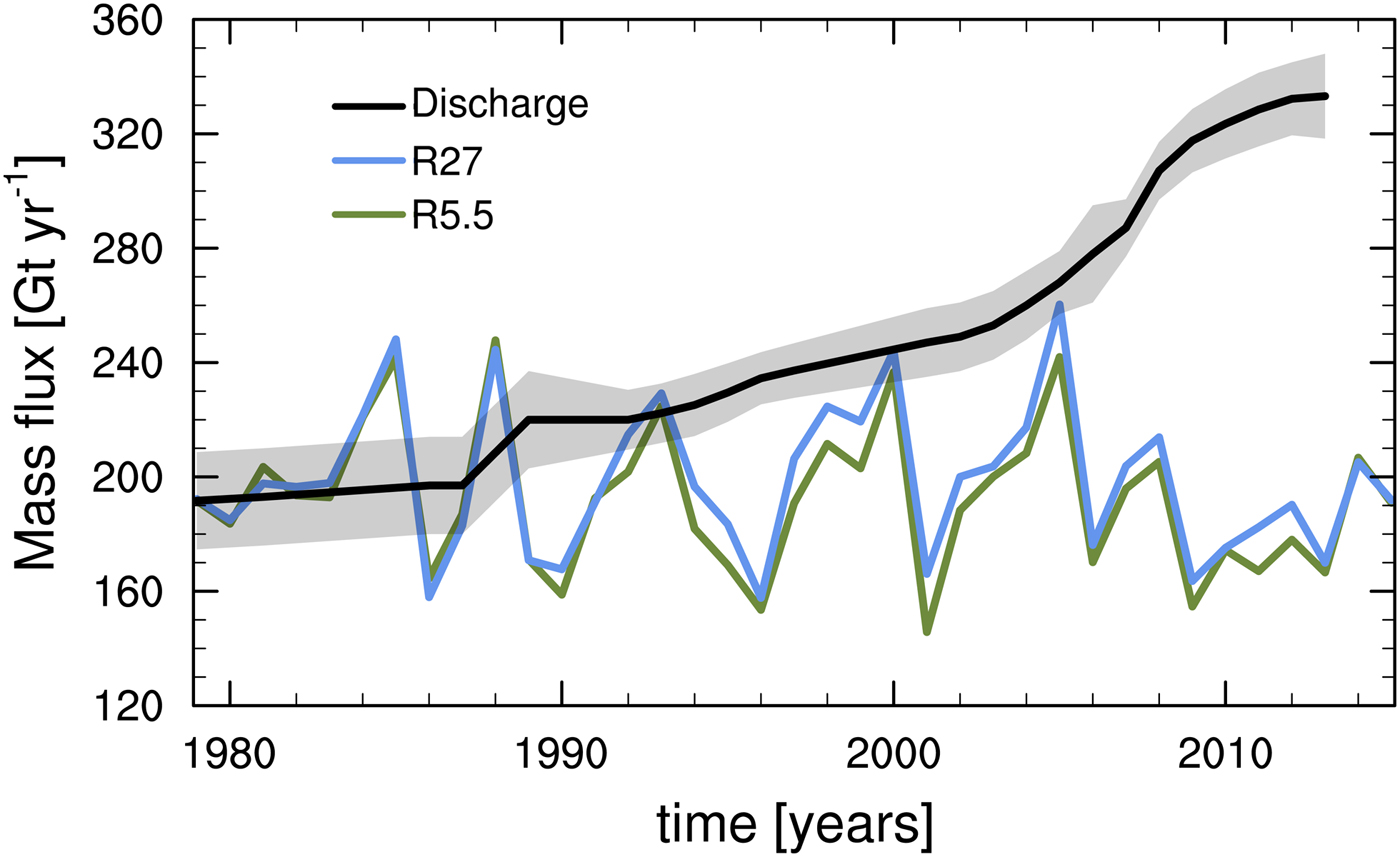
Our comparison with detailed observations clearly indicates that R5.5 and R27 simulate different SMB patterns on small spatial scales. In this regard, the question remains whether we need to resolve the climate at 5.5 km resolution to obtain a realistic area-integrated SMB flux. To answer this question, we integrated the R5.5 and R27 SMB over the whole ASE glacier area. This area, encompassing 428 000 km2, includes the Pine Island, Thwaites, Kohler, Smith and Pope glaciers. By differencing the cumulative solid ice flux along the grounding line of these glaciers (Mouginot and others, Reference Mouginot, Rignot and Scheuchl2014) with the area integrated SMB (Fig. 11), we can assess the mass balance of this area (Rignot and others, Reference Rignot, Velicogna, Van Den Broeke, Monaghan and Lenaerts2011). Up to the late 1980's, the ice flux and SMB were approximately equal, although strong SMB showed strong inter-annual variations, resulting in negative mass balance in low-SMB years (e.g. 1984 or 1988) and positive mass balance in high-SMB years (e.g. 1986). From then onwards, multi-annual SMB remains constant, while the ice discharge increases steadily from ~200 to 330 Gta−1. This has caused a series of negative mass balance years, with the exception of a few high-SMB years, when SMB and ice discharge cancelled out (1993, 2000, and 2005). Since 2005, the combination of high ice discharge and low SMB has led to strongly negative mass balance in each year (−150 to −100 Gta−1). If we compare area-integrated SMB from R5.5 and R27, we find very small differences (<20 Gta−1), approximately the same order of magnitude as the uncertainty in the ice discharge and the error traditionally assigned to SMB in mass balance studies (Depoorter and others, Reference Depoorter2013). This illustrates that RACMO2 applied at higher horizontal resolution does not give conclusive added value for basin-wide mass balance estimates.
Simulated (R5.5 in green, R27 in blue) annual area-integrated SMB (1979–2015) and ice discharge (1979–2013, taken from Mouginot and others, Reference Mouginot, Rignot and Scheuchl2014) of the Amundsen embayment glacier basins (see Fig. 1b for extent).
DISCUSSION AND CONCLUSIONS
Here we presented output from a high-resolution (5.5 km) regional atmospheric climate model (RACMO2) and assessed the performance of this model in comparison with a set of novel, so far partly undocumented observations, and with a version of RACMO2 with lower horizontal resolution (27 km).
Our analysis shows that the high-resolution model (R5.5) compares very well with observations of near-surface climate, surface melt and SMB. It substantially outperforms the low-resolution model (R27) for both 2-m temperature and 10-m wind speed. Especially for coastal stations, the enhanced topographical detail helps to better simulate the temperature and wind climate. Although the absolute values of surface melt are underestimated, the spatial patterns, extent, and interannual variability are very well simulated by R5.5. For SMB, we found a mixed signal, with better performance of R5.5 over the Pine Island Glacier, but an overall negative bias at interior sites. R27, on the other hand, very well represents SMB in comparison with interior firn core records.
In the coastal regions, we find very high simulated SMB on the windward side of topographic features in R5.5, which are partly confirmed by airborne radar observations. However, significant biases are found in the simulated absolute SMB values, as well as the location of the SMB maximum on the windward slope. These results suggest that, employed at this resolution, RACMO2 produces excessive orographic snowfall rates, which, in return, lead to a dry bias in parts of the interior ice sheet. In contrast, R27 does not resolve these smaller topographic features and related snowfall patterns, but generates a coast-interior SMB gradient that appears to be equally, if not more, consistent with observations.
Overall, the high resolution in RACMO2 resolves small-scale climate, surface melt and SMB patterns that are not resolved by lower-resolution models, reanalyses and observational datasets (Medley and others, Reference Medley2013). This dataset can therefore prove useful to aid in the choice of an ice core location, in understanding regional near-surface climate variability, and in forcing high-resolution ice-sheet and/or ocean models. Moreover, altimetry estimates of ice sheet elevation change resolve the detailed pattern of change; however, an outstanding challenge is how to convert from volume to mass. One approach is to correct the altimetry-derived rate of elevation change for elevation change associated with surface processes (Ligtenberg and others, Reference Ligtenberg, Helsen and van den Broeke2011; Wouters and others, Reference Wouters2015), but any error in either the data or the correction will then be converted to mass change at the density of ice, leading to a bias in the final result (Hogg and others, Reference Hogg2017). In the future, we recommend that the high spatial resolution R5.5 SMB is used as the input for a high-resolution firn compaction model, which may improve the accuracy with which we can partition surface mass and dynamically induced elevation change. However, one should be cautious when using this dataset around small-scale coastal topography, where model biases remain substantial.
Ongoing and future RACMO2 development should focus on reducing the bias of orographic precipitation. In particular, RACMO2 currently does not calculate precipitation prognostically, which implies that snow falls in the same grid cell as it was generated. Employed at horizontal grid sizes smaller than the typical distance between in-cloud snow grain formation and snowfall (10–20 km), this will inevitably lead to biases in the location of SMB maxima in high-precipitation regions, such as coastal domes. Additionally, RACMO2 uses the hydrostatic approximation, which might explain some of the biases found in the high-resolution model. Atmospheric processes at spatial scales similar to the R5.5 grid size that drive high vertical velocities and vigorous mixing, such as strong convection along the steep slopes inward of the ice-shelf grounding lines and orographic lifting on windward sides of coastal domes, might be poorly represented. Therefore, future work should also target developing non-hydrostatic models for this application.
DATA AVAILABILITY
RACMO2 data are available by request to the corresponding author (Jan.Lenaerts@colorado.edu). AWS data are available through the AMRC and Automatic Weather Station (AWS) program. Surface melt datasets are available from L. D. Trusel (trusel@rowan.edu) and J. P. Nicolas (nicolas.7@osu.edu). The firn core records collated for the Antarctica 2k project are available at the UK Polar Data centre or by request from E. R. Thomas (lith@bas.ac.uk). Operation IceBridge SMB data are available from Brooke Medley (brooke.c.medley@nasa.gov). The observations of SMB along the iSTAR traverse are available on request from Anna Hogg (A.E.Hogg@leeds.ac.uk).
SUPPLEMENTARY MATERIAL
The supplementary material for this article can be found at https://doi.org/10.1017/aog.2017.42.
ACKNOWLEDGMENTS
J. T. M. L. and S. R. M. L. are funded by the Netherlands Science Organization through the Innovational Research Incentives Scheme Veni. H. K., R. M., R. J. T. and A. E. H. were supported by the UK Natural Environment Research Council's iSTAR Programme. The authors appreciate the support of the University of Wisconsin-Madison Automatic Weather Station Program for the data set, data display and information, NSF grant number ANT-1543305, and of the iSTAR management and field logistics. Data analysis and plotting were performed using the the NCAR Command Language (UCAR/NCAR/CISL/VETS, 2014) and the QGIS Quantarctica package developed by the Norwegian Polar Institute.


 Open access