2. Adjoint-descent method for constructing equilibrium solutions

Consider a general autonomous dynamical system

(2.1)\begin{equation} \dfrac{\partial\boldsymbol{u}}{\partial t} = \boldsymbol{r}(\boldsymbol{u}), \end{equation}

where $\boldsymbol {u}$ is an $n$-dimensional real-valued field defined over a $d$-dimensional spatial domain $\boldsymbol {x}\in \varOmega \subseteq \mathbb {R}^d$ and varying with time $t\in \mathbb {R}$. Within the space of vector fields $\mathscr {M}=\{\boldsymbol {u}:\varOmega \to \mathbb {R}^n\}$, the evolution of $\boldsymbol {u}$ is governed by the smooth nonlinear operator $\boldsymbol {r}$ subject to time-independent boundary conditions (BCs) at $\partial \varOmega$, the boundary of $\varOmega$. Equilibrium solutions of this dynamical system are $\boldsymbol {u}^\ast \in \mathscr {M}$ for which

(2.2)\begin{equation} \boldsymbol{r}(\boldsymbol{u}^\ast) = \boldsymbol{0}. \end{equation}

The residual of (2.2) is not zero for non-equilibrium states $\boldsymbol {u}\neq \boldsymbol {u}^\ast$. We thus penalise non-equilibrium states by the non-negative cost function $J^2$ defined as

(2.3)\begin{equation} J^2 = \left\langle\boldsymbol{r}(\boldsymbol{u}),\boldsymbol{r}(\boldsymbol{u})\right\rangle, \end{equation}

where $\left \langle \cdot,\cdot \right \rangle$ denotes an inner product defined on $\mathscr {M}$. The cost function takes zero value if and only if $\boldsymbol {u}=\boldsymbol {u}^\ast$. We thereby recast the problem of finding equilibrium solutions $\boldsymbol {u}^\ast$ as a minimisation problem over $\mathscr {M}$, and look for the global minima of $J^2$ at which $J^2=0$, following the arguments of Farazmand (Reference Farazmand2016).

In order to find minima of $J^2$, we construct another dynamical system in $\mathscr {M}$ along whose evolution the cost function $J^2$ decreases monotonically. The objective is to define an evolution equation

(2.4)\begin{equation} \dfrac{\partial\boldsymbol{u}}{\partial\tau}=\boldsymbol{g}(\boldsymbol{u}), \end{equation}

where the choice of the operator $\boldsymbol {g}$ guarantees

(2.5)\begin{equation} \dfrac{\partial J^2}{\partial\tau}\leq 0, \quad \forall\tau. \end{equation}

Here, $\tau$ is a fictitious time that parametrises the evolution governed by the constructed dynamics. The rate of change of $J^2$ along trajectories of the dynamical system (2.4) is

(2.6)\begin{equation} \dfrac{\partial J^2}{\partial\tau} = 2\left\langle\mathscr{L}(\boldsymbol{u};\boldsymbol{g}),\boldsymbol{r}(\boldsymbol{u})\right\rangle, \end{equation}

where $\mathscr {L}(\boldsymbol {u};\boldsymbol {g})$ is the directional derivative of $\boldsymbol {r}(\boldsymbol {u})$ along $\partial \boldsymbol {u}/\partial \tau =\boldsymbol {g}$:

(2.7)\begin{equation} \mathscr{L}(\boldsymbol{u};\boldsymbol{g}) = \lim_{\epsilon\to0}\dfrac{\boldsymbol{r}(\boldsymbol{u}+\epsilon\boldsymbol{g})-\boldsymbol{r}(\boldsymbol{u})}{\epsilon}. \end{equation}

We can rewrite (2.6) as

(2.8)\begin{equation} \dfrac{\partial J^2}{\partial\tau} = 2\left\langle\mathscr{L}^{\dagger}(\boldsymbol{u};\boldsymbol{r}),\boldsymbol{g}(\boldsymbol{u})\right\rangle, \end{equation}

where $\mathscr {L}^{\dagger}$ is the adjoint operator of the directional derivative $\mathscr {L}$, with the following definition:

(2.9)\begin{equation} \left\langle\mathscr{L}(\boldsymbol{v};\boldsymbol{v}'),\boldsymbol{v}''\right\rangle=\left\langle\mathscr{L}^{\dagger}(\boldsymbol{v};\boldsymbol{v}''),\boldsymbol{v}'\right\rangle , \quad \forall\ \boldsymbol{v},\boldsymbol{v}',\boldsymbol{v}''\in\mathscr{M}. \end{equation}

To guarantee the monotonic decrease of $J^2$ with $\tau$, we choose

(2.10)\begin{equation} \boldsymbol{g}(\boldsymbol{u}) ={-}\mathscr{L}^{\dagger}(\boldsymbol{u};\boldsymbol{r}). \end{equation}

This choice results in monotonic decrease of $J^2$ along solution trajectories of the adjoint dynamical system (2.4):

(2.11)\begin{equation} \dfrac{\partial J^2}{\partial\tau} ={-}2\left\langle\mathscr{L}^{\dagger}(\boldsymbol{u};\boldsymbol{r}),\mathscr{L}^{\dagger}(\boldsymbol{u};\boldsymbol{r})\right\rangle\leq 0. \end{equation}

In summary, in order to find equilibria of $\partial \boldsymbol {u}/\partial t=\boldsymbol {r}(\boldsymbol {u})$, the variational approach proposed by Farazmand (Reference Farazmand2016) constructs a globally contracting dynamical system $\partial \boldsymbol {u}/\partial \tau =\boldsymbol {g}(\boldsymbol {u})$ that is essentially the gradient descent of the cost function $J^2$. Every trajectory of the constructed dynamical system eventually reaches a stable equilibrium corresponding to a minimum of the cost function. Equilibria of the original dynamics are equilibria of the adjoint dynamics at which the cost function takes its global minimum value $J^2=0$. 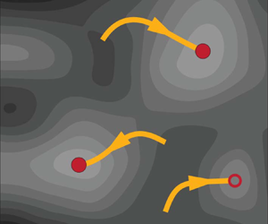However, the adjoint dynamics might have other equilibria that correspond to a local minimum of the cost function with $J^2>0$, and are not equilibria of the original dynamics. This is illustrated schematically in figure 1. Finding equilibria of $\partial \boldsymbol {u}/\partial t=\boldsymbol {r}(\boldsymbol {u})$ requires integrating the adjoint dynamics $\partial \boldsymbol {u}/\partial \tau =\boldsymbol {g}(\boldsymbol {u})$ forwards in the fictitious time $\tau$. The solutions obtained at $\tau \to \infty$ for which $J^2=0$ are equilibria of the original system. Otherwise, when the trajectory gets stuck in a local minimum of the cost function, the search fails and the adjoint dynamics should be integrated from another initial condition.

Figure 1.

Replacing the original dynamics with the gradient descent of the cost function $J=\|\boldsymbol {r}(\boldsymbol {u})\|$ by the adjoint-descent method. (a) Schematic of the trajectories and two equilibria of the original system parametrised by the physical time $t$: $\partial \boldsymbol {u}/\partial t=\boldsymbol {r}(\boldsymbol {u})$. (b) Contours of $J$ and sample trajectories of its gradient flow parametrised by the fictitious time $\tau$: $\partial \boldsymbol {u}/\partial \tau =\boldsymbol {g}(\boldsymbol {u})$. Trajectories of the adjoint-descent dynamics converge to a stable fixed point, that is, either an equilibrium of the original dynamics, where the global minimum value of $J=0$ is achieved, or a state at which $J$ takes a local minimum value.

3. Application to the wall-bounded shear flows

3.1. Governing equations

We consider the flow in a 3-D rectangular domain $\varOmega$ of non-dimensional size $x\in [0,L_x)$, $y\in [-1,+1]$ and $z\in [0,L_z)$. The domain is bounded in $y$ between two parallel plates, and is periodic in the lateral directions $x$ and $z$. Incompressible isotherm flow of a Newtonian fluid is governed by the Navier–Stokes equations (NSE). The non-dimensional, perturbative form of the NSE reads

(3.1)$$\begin{gather} \frac{\partial\boldsymbol{u}}{\partial t}={-}\left[(\boldsymbol{u}_b\boldsymbol{\cdot}\boldsymbol{\nabla})\boldsymbol{u}+(\boldsymbol{u}\boldsymbol{\cdot}\boldsymbol{\nabla})\boldsymbol{u}_b+(\boldsymbol{u}\boldsymbol{\cdot}\boldsymbol{\nabla})\boldsymbol{u}\right]-\boldsymbol{\nabla} p+\frac{1}{Re}\,\Delta\boldsymbol{u}=:\mathcal{F}(\boldsymbol{u},p), \end{gather}$$

(3.2)$$\begin{gather}\boldsymbol{\nabla}\boldsymbol{\cdot}\boldsymbol{u}=0. \end{gather}$$

Here, $Re$ is the Reynolds number, and $\boldsymbol {u}_b$ is the laminar base flow velocity field. The fields $\boldsymbol {u}$ and $p$ are the deviations of the total velocity and pressure from the base flow velocity and pressure fields, respectively. For common driving mechanisms such as the motion of walls in the $xz$ plane, externally imposed pressure differences, or injection/suction through the walls, the laminar base flow satisfies the inhomogeneous BCs, absorbs body forces, and is known a priori. Consequently, the perturbative NSE (3.1) and (3.2) are subject to the BCs

(3.3)$$\begin{gather} \boldsymbol{u}(x,y=\pm1,z;t)=\boldsymbol{0}, \end{gather}$$

(3.4)$$\begin{gather}{}[\boldsymbol{u},p](x=0,y,z;t)=[\boldsymbol{u},p](x=L_x,y,z;t), \end{gather}$$

(3.5)$$\begin{gather}{}[\boldsymbol{u},p](x,y,z=0;t)=[\boldsymbol{u},p](x,y,z=L_z;t). \end{gather}$$

The canonical wall-bounded shear flows such as PCF, plane Poiseuille flow and asymptotic suction boundary layer flow are governed by the incompressible NSE (3.1)–(3.5), where $\boldsymbol {u}_b$ differentiates them from one another. We derive the adjoint-descent dynamics based on a general base flow velocity field $\boldsymbol {u}_b$, and in § 5 demonstrate the adjoint-based method for the specific case of PCF.

The state space $\mathscr {M}$ of the NSE contains velocity fields $\boldsymbol {u}:\varOmega \to \mathbb {R}^3$ of zero divergence that satisfy the kinematic conditions (3.3)–(3.5). The space $\mathscr {M}$ carries the standard energy-based $L_2$ inner product denoted with $\left \langle \cdot,\cdot \right \rangle _\mathscr {M}$. The pressure $p$ associated with an admissible velocity field $\boldsymbol {u}\in \mathscr {M}$ ensures that under the NSE dynamics, the velocity remains divergence-free,

(3.6)\begin{equation} \partial(\boldsymbol{\nabla}\boldsymbol{\cdot}\boldsymbol{u})/\partial t = \boldsymbol{\nabla}\boldsymbol{\cdot}\mathcal{F}(\boldsymbol{u},p) = 0, \end{equation}

while remaining compatible with the no-slip BCs (3.3),

(3.7)\begin{equation} \left.\partial\boldsymbol{u}/\partial t\right|_{y=\pm1} = \left.\mathcal{F}(\boldsymbol{u},p)\right|_{y=\pm1} = \boldsymbol{0}. \end{equation}

This requires $p$ to satisfy the Poisson equation with a velocity-dependent source term (Rempfer Reference Rempfer2006; Canuto et al. Reference Canuto, Hussaini, Quarteroni and Zang2007).

We could not derive a variational dynamics based on expressing pressure explicitly as the solution to this Poisson equation. Therefore, instead of the state space $\mathscr {M}$ of the NSE, we define the search space such that ‘velocity’ and ‘pressure’ can evolve independently. Accordingly, we define the cost function such that residuals of both (3.1) and (3.2) are included. Otherwise, the derivation follows § 2.

3.2. The search space

We define the inner product space of general flow fields as

(3.8)\begin{equation} \mathscr{P}=\left\{\begin{bmatrix} \boldsymbol{v}\\ q \end{bmatrix}\left| \begin{array}{@{}c@{}} \boldsymbol{v}:\varOmega \rightarrow \mathbb{R}^3\\ q:\varOmega \rightarrow \mathbb{R}\\ \boldsymbol{v} \text{ and } q \text{ periodic in } x \text{ and } z \end{array}\right.\right\}, \end{equation}

where $\boldsymbol {v}$ and $q$ are sufficiently smooth functions of space. Hereafter, the symbols $\boldsymbol {u},p$ indicate physically admissible velocity and pressure, implying $\boldsymbol {u}\in \mathscr {M}$ and $p$ satisfying the relevant Poisson equation. The space of general flow fields $\mathscr {P}$ is endowed with the real-valued inner product

(3.9) \begin{align} \left\langle\cdot ,\cdot \right\rangle:\mathscr{P} \times \mathscr{P}\rightarrow \mathbb{R}, \left\langle \begin{bmatrix} \boldsymbol{v}_1\\ q_1 \end{bmatrix} , \begin{bmatrix} \boldsymbol{v}_2\\ q_2 \end{bmatrix} \right\rangle=\int_\varOmega\left(\boldsymbol{v}_1\boldsymbol{\cdot}\boldsymbol{v}_2+q_1q_2\right)\text{d}\kern0.7pt \boldsymbol{x}. \end{align}

Here, $\boldsymbol {\cdot }$ is the conventional Euclidean inner product in $\mathbb {R}^3$. Physically admissible velocity and pressure fields form the following subset of the general flow fields:

(3.10)\begin{equation} \mathscr{P}_p=\left\{ \begin{bmatrix} \boldsymbol{u}\\ p \end{bmatrix}\in\mathscr{P}_0\left| \begin{array}{@{}c@{}} \boldsymbol{\nabla}\boldsymbol{\cdot}\boldsymbol{u}=0\\ \boldsymbol{\nabla}\boldsymbol{\cdot}\mathcal{F}(\boldsymbol{u},p) = 0\\ \mathcal{F}(\boldsymbol{u},p)\big|_{y=\pm1} = \boldsymbol{0} \end{array}\right.\right\}, \end{equation}

where $\mathscr {P}_0$ is the subset of $\mathscr {P}$ whose vector-valued component satisfies the homogeneous Dirichlet BC at the walls,

(3.11)\begin{equation} \mathscr{P}_0=\left\{ \begin{bmatrix} \boldsymbol{v}\\ q \end{bmatrix}\in\mathscr{P}\;\bigg|\; \boldsymbol{v}(y=\pm1)=\boldsymbol{0}\right\}. \end{equation}

Equilibrium solutions of the NSE are $[\boldsymbol {u}^\ast,p^\ast ]\in \mathscr {P}_p$ for which

(3.12)\begin{equation} \mathcal{F}(\boldsymbol{u}^\ast,p^\ast)=\boldsymbol{0}. \end{equation}

We aim to impose the zero-divergence constraint together with the defining property of an equilibrium solution via the variational minimisation discussed in § 2. To that end, we consider an evolution in the space of general flow fields $\boldsymbol {U}=[\boldsymbol {v},q]\in \mathscr {P}_0$ in which the velocity and the pressure component are evolved independently. A flow field $\boldsymbol {U}\in \mathscr {P}_0$ necessarily satisfies neither the defining property of an equilibrium solution nor the zero-divergence constraint. Therefore, we define the residual field $\boldsymbol {R}\in \mathscr {P}$ associated with a general flow field as

(3.13)\begin{equation} \boldsymbol{R}=\begin{bmatrix} \boldsymbol{r}_1\\ r_2 \end{bmatrix}=\begin{bmatrix} \mathcal{F}(\boldsymbol{v},q)\\ \boldsymbol{\nabla}\boldsymbol{\cdot}\boldsymbol{v} \end{bmatrix}, \end{equation}

and the cost function $J^2$ as

(3.14)\begin{equation} J^2 = \int_\varOmega\left(\mathcal{F}^2(\boldsymbol{v},q)+\left(\boldsymbol{\nabla}\boldsymbol{\cdot}\boldsymbol{v}\right)^2\right)\text{d}\kern0.7pt \boldsymbol{x} = \int_\varOmega\left(\boldsymbol{r}_1\boldsymbol{\cdot}\boldsymbol{r}_1+r_2^2\right)\text{d}\kern0.7pt \boldsymbol{x} = \left\langle\boldsymbol{R},\boldsymbol{R}\right\rangle. \end{equation}

At the global minima of the cost function, $J^2=0$, the defining property of an equilibrium solution (3.12) and the incompressibility constraint (3.2) are both satisfied. The operator $\boldsymbol {G}=[\boldsymbol {g}_1,g_2]$ acting on general flow fields $\boldsymbol {U}=[\boldsymbol {v},q]\in \mathscr {P}_0$ is constructed such that an equilibrium solution $[\boldsymbol {u}^\ast,p^\ast ]$ is obtained by evolving the variational dynamics

(3.15)\begin{equation} \dfrac{\partial\boldsymbol{U}}{\partial\tau} = \dfrac{\partial}{\partial\tau} \begin{bmatrix} \boldsymbol{v}\\ q \end{bmatrix}= \begin{bmatrix} \boldsymbol{g}_1\\ g_2 \end{bmatrix}. \end{equation}

The operator $\boldsymbol {G}$ is derived following the adjoint-based method described in § 2 to guarantee the monotonic decrease of the cost function along trajectories of the variational dynamics (3.15).

3.3. Adjoint operator for the NSE

The variational dynamics (3.15) must ensure that the flow field $\boldsymbol {U}$ remains within $\mathscr {P}_0$, thus $\boldsymbol {U}$ is periodic in $x$ and $z$, and its velocity component $\boldsymbol {v}$ takes zero value at the walls for all $\tau$. In order for these properties of $\boldsymbol {U}$ to be preserved under the variational dynamics, the operator $\boldsymbol {G}$ must be periodic in $x$ and $z$, and $\boldsymbol {g}_1=\partial \boldsymbol {v}/\partial \tau$ must take zero value at the walls, meaning that $\boldsymbol {G}\in \mathscr {P}_0$. In addition, we choose the residual $\boldsymbol {R}$ to lie within $\mathscr {P}_0$. The periodicity of $\boldsymbol {R}$ in $x$ and $z$ results automatically from the spatial periodicity of $\boldsymbol {U}$ in these two directions. However, at the walls we enforce the condition $\boldsymbol {r}_1(\boldsymbol {v},q)|_{y=\pm 1}=\mathcal {F}(\boldsymbol {v},q)|_{y=\pm 1}=\boldsymbol {0}$. With the choice of $\boldsymbol {U},\boldsymbol {R},\boldsymbol {G}\in \mathscr {P}_0$, the flow field remains within $\mathscr {P}_0$ as desired. Following this choice, all the boundary terms resulting from partial integrations in the derivation of the adjoint operator cancel out (see Appendix A), and the adjoint of the directional derivative of $\boldsymbol {R}(\boldsymbol {U})$ along $\boldsymbol {G}$ is obtained as

(3.16)$$\begin{gather} \mathscr{L}^{\dagger}_1 = \left(\boldsymbol{\nabla}\boldsymbol{r}_1\right)\left(\boldsymbol{u}_b+\boldsymbol{v}\right)-\left(\boldsymbol{\nabla}(\boldsymbol{u}_b+\boldsymbol{v})\right)^{\rm T}\boldsymbol{r}_1+\dfrac{1}{Re}\,\Delta\boldsymbol{r}_1+r_2\boldsymbol{r}_1-\boldsymbol{\nabla} r_2, \end{gather}$$

(3.17)$$\begin{gather}\mathscr{L}^{\dagger}_2 = \boldsymbol{\nabla}\boldsymbol{\cdot}\boldsymbol{r}_1. \end{gather}$$

Therefore, with $\boldsymbol {G}=-\mathscr {L}^{\dagger} (\boldsymbol {U};\boldsymbol {R})$, the variational dynamics takes the form

(3.18)$$\begin{gather} \dfrac{\partial\boldsymbol{v}}{\partial\tau}={-}\mathscr{L}^{\dagger}_1 ={-}\left(\boldsymbol{\nabla}\boldsymbol{r}_1\right)\left(\boldsymbol{u}_b+\boldsymbol{v}\right)+\left(\boldsymbol{\nabla}(\boldsymbol{u}_b+\boldsymbol{v})\right)^{\rm T}\boldsymbol{r}_1-\dfrac{1}{Re}\,\Delta\boldsymbol{r}_1-r_2\boldsymbol{r}_1+\boldsymbol{\nabla} r_2, \end{gather}$$

(3.19)$$\begin{gather}\dfrac{\partial q}{\partial \tau}={-}\mathscr{L}^{\dagger}_2 ={-}\boldsymbol{\nabla}\boldsymbol{\cdot}\boldsymbol{r}_1. \end{gather}$$

Equation (3.18) is fourth order with respect to $\boldsymbol {v}$, and (3.19) is second order with respect to $q$. Therefore, four BCs for each component of $\boldsymbol {v}$ and two BCs for $q$ are required in the inhomogeneous direction $y$. The choice of $\boldsymbol {U}\in \mathscr {P}_0$ implies $\boldsymbol {v}=\boldsymbol {0}$, and the choice of $\boldsymbol {R}\in \mathscr {P}_0$ implies $\boldsymbol {r}_1=\mathcal {F}(\boldsymbol {v},q)=\boldsymbol {0}$ at each wall. Consequently, the adjoint-descent dynamics requires two additional wall BCs in order to be well-posed. As the additional BCs, we impose $\boldsymbol {\nabla }\boldsymbol {\cdot }\boldsymbol {v}=0$ at each wall. Therefore, the adjoint-descent dynamics is subject to the following BCs:

(3.20)$$\begin{gather} [\boldsymbol{v},q](x=0,y,z;\tau)=[\boldsymbol{v},q](x=L_x,y,z;\tau), \end{gather}$$

(3.21)$$\begin{gather}{}[\boldsymbol{v},q](x,y,z=0;\tau)=[\boldsymbol{v},q](x,y,z=L_z;\tau), \end{gather}$$

(3.22)$$\begin{gather}\boldsymbol{v}(x,y=\pm1,z;\tau)=\boldsymbol{0}, \end{gather}$$

(3.23)$$\begin{gather}\left[-\boldsymbol{u}_b\boldsymbol{\cdot}\boldsymbol{\nabla}\boldsymbol{v} - \boldsymbol{\nabla} q+\frac{1}{Re}\,\Delta\boldsymbol{v} \right]_{y=\pm1}=\boldsymbol{0}, \end{gather}$$

(3.24)$$\begin{gather}\left.\boldsymbol{e}_y\boldsymbol{\cdot}\dfrac{\partial\boldsymbol{v}}{\partial y}\right|_{y=\pm1} = 0, \end{gather}$$

where the BC (3.23) is $\boldsymbol {r}_1=\mathcal {F}(\boldsymbol {v},q)=\boldsymbol {0}$, and the BC (3.24) is $\boldsymbol {\nabla }\boldsymbol {\cdot }\boldsymbol {v}=0$ at the walls obtained by substituting $\boldsymbol {v}(y=\pm 1)=\boldsymbol {0}$ in the definitions of $\mathcal {F}(\boldsymbol {v},q)$ and $\boldsymbol {\nabla }\boldsymbol {\cdot }\boldsymbol {v}$, respectively. The choice of the additional BCs is consistent with the properties of the state space of the NSE, and is physically meaningful. Note, however, that the BC (3.24) does not need to be enforced explicitly during the derivation of the adjoint operator. In the absence of solid walls in a doubly periodic 2-D or a triply periodic 3-D domain, the BCs (3.22)–(3.24) do not apply. Instead, the fields are subject to periodic BCs only.

Numerically imposing the BCs (3.22)–(3.24) while evolving (3.18) and (3.19) forwards in the fictitious time is not straightforward. Consequently, instead of advancing the derived variational dynamics directly, we constrain the adjoint-descent dynamics to the subset of physical flow fields $\mathscr {P}_p$. Within this subset, pressure does not evolve independently but satisfies the pressure Poisson equation. Thereby, we obtain an evolution equation for the velocity within the state space of the NSE. This allows us to employ the influence matrix (IM) method (Kleiser & Schumann Reference Kleiser and Schumann1980) to integrate the constrained adjoint-descent dynamics.

3.4. Variational dynamics constrained to the subset of physical flow fields

To obtain a numerically tractable variational dynamics, we constrain the adjoint-descent dynamics (3.18)–(3.24) to the subset of physical flow fields $\mathscr {P}_p$. Within $\mathscr {P}_p$, the velocity component $\boldsymbol {u}$ is divergence-free over the entire domain. In addition, the pressure component $p$ is governed no longer by an explicit evolution equation, but by a Poisson equation with a velocity-dependent source term. Let $p = \mathcal {P}[\boldsymbol {u}]$ denote the solution to the Poisson equation yielding pressure associated with an instantaneous divergence-free velocity $\boldsymbol {u}$. In order for $\boldsymbol {u}$ to remain divergence-free, $\boldsymbol {g}_1$ needs to be projected onto the space of divergence-free fields, yielding the evolution

(3.25)\begin{equation} \dfrac{\partial\boldsymbol{u}}{\partial\tau} = \mathbb{P}\left\{ -\left(\boldsymbol{\nabla}\boldsymbol{r}_1\right)\left(\boldsymbol{u}_b+\boldsymbol{u}\right)+\left(\boldsymbol{\nabla}(\boldsymbol{u}_b+\boldsymbol{u})\right)^{\rm T}\boldsymbol{r}_1-\dfrac{1}{Re}\,\Delta\boldsymbol{r}_1\right\}=:\boldsymbol{f}, \end{equation}

where $\mathbb {P}$ denotes the projection operator. The argument of the operator $\mathbb {P}$ is the right-hand side of (3.18) with $r_2=0$ and $\boldsymbol {\nabla } r_2=\boldsymbol {0}$ that result from the zero divergence of $\boldsymbol {u}$. According to Helmholtz's theorem, a smooth 3-D vector field can be decomposed into divergence-free and curl-free components. Thus $\boldsymbol {g}_1=\partial \boldsymbol {u}/\partial \tau$ is decomposed as $\boldsymbol {g}_1=\boldsymbol {f} - \boldsymbol {\nabla } \phi$, where $\boldsymbol {f}=\mathbb {P}\{\boldsymbol {g}_1\}$ is the divergence-free component, and $\phi$ is the scalar potential whose gradient gives the curl-free component. Therefore, the evolution of the divergence-free velocity is governed by

(3.26)$$\begin{gather} \dfrac{\partial\boldsymbol{u}}{\partial\tau} ={-}\left(\boldsymbol{\nabla}\boldsymbol{r}_1\right)\left(\boldsymbol{u}_b+\boldsymbol{u}\right)+\left(\boldsymbol{\nabla}(\boldsymbol{u}_b+\boldsymbol{u})\right)^{\rm T}\boldsymbol{r}_1+\boldsymbol{\nabla}\phi-\dfrac{1}{Re}\,\Delta\boldsymbol{r}_1, \end{gather}$$

(3.27)$$\begin{gather}\boldsymbol{\nabla}\boldsymbol{\cdot}\boldsymbol{u}=0, \end{gather}$$

subject to

(3.28)$$\begin{gather} \boldsymbol{u}(x=0,y,z;\tau)=\boldsymbol{u}(x=L_x,y,z;\tau), \end{gather}$$

(3.29)$$\begin{gather}\boldsymbol{u}(x,y,z=0;\tau)=\boldsymbol{u}(x,y,z=L_z;\tau), \end{gather}$$

(3.30)$$\begin{gather}\boldsymbol{u}(x,y=\pm1,z;\tau)=\boldsymbol{0}, \end{gather}$$

(3.31)$$\begin{gather}\boldsymbol{r}_1(x,y=\pm1,z;\tau)=\boldsymbol{0}, \end{gather}$$

where $\boldsymbol {r}_1=\boldsymbol {r}_1(\boldsymbol {u},\mathcal {P}[\boldsymbol {u}])$ and thus the BC (3.31) is satisfied automatically. It is necessary to verify that the constrained variational dynamics still guarantees a monotonic decrease of the cost function. For $\boldsymbol {U}\in \mathscr {P}_p$, the scalar component of the steepest descent direction, $g_2$, vanishes (see (3.19)). Therefore, according to the definition of the inner product on $\mathscr {P}_p$ (3.9), it is sufficient to verify that $\int _\varOmega (\boldsymbol {f}\boldsymbol {\cdot }\boldsymbol {g}_1)\,\mathrm {d}\kern0.7pt \boldsymbol {x}=\left \langle \boldsymbol {f},\boldsymbol {g}_1\right \rangle _\mathscr {M}\geq 0$. The Helmholtz decomposition is an orthogonal decomposition with respect to the $L_2$ inner product defined on the state space of the NSE, $\left \langle \boldsymbol {f},\boldsymbol {\nabla }\phi \right \rangle _\mathscr {M}= 0$. Therefore, $\left \langle \boldsymbol {f},\boldsymbol {g}_1\right \rangle _\mathscr {M}=\left \langle \boldsymbol {f},\boldsymbol {f}\right \rangle _\mathscr {M}-\left \langle \boldsymbol {f},\boldsymbol {\nabla }\phi \right \rangle _\mathscr {M}=\|\boldsymbol {f}\|^2_\mathscr {M}\geq 0$, thus the evolution of $\boldsymbol {u}$ along $\boldsymbol {f}$ guarantees the monotonic decrease of the cost function, as desired.

The variational dynamics (3.26)–(3.31) is equivariant under continuous translations in the periodic directions $x$ and $z$. Furthermore, one can verify through simple calculations that this dynamics is also equivariant under the action of any reflection or rotation permitted by the laminar base velocity field $\boldsymbol {u}_b$. Consequently, the symmetry group generated by translations, reflections and rotations in the obtained variational dynamics is identical to that of the NSE (3.1)–(3.5). Therefore, to construct equilibria within a particular symmetry-invariant subspace of the NSE, one can use initial conditions from the same symmetry-invariant subspace to initialise the variational dynamics, and the variational dynamics preserves the symmetries of the initial condition.

In the variational dynamics, the scalar field $\phi$ plays a role analogous to the pressure $p$ in the incompressible NSE. The scalar fields $\phi$ and $p$ adjust themselves to the instantaneous physical velocity $\boldsymbol {u}$ such that $\boldsymbol {\nabla }\boldsymbol {\cdot }\boldsymbol {u}=0$ and $\boldsymbol {u}(y=\pm 1)=\boldsymbol {0}$ are preserved under the evolution with the fictitious time $\tau$ and the physical time $t$, respectively. Similar to the pressure in the NSE, $\phi$ satisfies a Poisson equation with a velocity-dependent source term. Solving the Poisson equation for $\phi$ and $p$ is a numerically challenging task in the present wall-bounded configuration (Rempfer Reference Rempfer2006). Therefore, instead of attempting to compute $p$ and $\phi$ and thereby advancing the variational dynamic (3.26), we formulate the numerical integration scheme based on the IM method (Kleiser & Schumann Reference Kleiser and Schumann1980), where the no-slip BC and zero divergence are satisfied precisely, while the explicit construction of $p$ and $\phi$ is circumvented.

4. Numerical implementation

To advance the variational dynamics (3.26)–(3.31) without computing explicitly $\phi$ and $p$, we take advantage of the structural similarity between the variational dynamics and the NSE. In order to evaluate the right-hand side of (3.26), we consider the following partial differential equation for the residual field $\boldsymbol {r}_1$:

(4.1)\begin{equation} \dfrac{\partial\boldsymbol{r}_1}{\partial\hat{\tau}}={-}\left(\boldsymbol{N}(\boldsymbol{r}_1)-\boldsymbol{\nabla}\phi+\dfrac{1}{Re}\,\Delta\boldsymbol{r}_1\right), \end{equation}

subject to

(4.2)$$\begin{gather} \boldsymbol{r}_1(y=\pm1)=\boldsymbol{0}, \end{gather}$$

(4.3)$$\begin{gather}\boldsymbol{\nabla}\boldsymbol{\cdot}\boldsymbol{r}_1=0, \end{gather}$$

where $\boldsymbol {N}(\boldsymbol {r}_1)=(\boldsymbol {\nabla }\boldsymbol {r}_1)(\boldsymbol {u}_b+\boldsymbol {u})-(\boldsymbol {\nabla }(\boldsymbol {u}_b+\boldsymbol {u}))^\textrm {T}\boldsymbol {r}_1$, with both $\boldsymbol {u}$ and $\boldsymbol {u}_b$ being treated as constant fields. We use the dummy equation (4.1) to evaluate the right-hand side of (3.26) since the instantaneously evaluated right-hand sides of these two systems are identically equal. For brevity, we are omitting the periodic BCs in $x$ and $z$ since spatial periodicity can be enforced via spectral representation in an appropriate basis, such as a Fourier basis, that is periodic by construction. Equation (4.1) together with the BC (4.2) and the zero-divergence constraint (4.3) resembles the structure of the incompressible NSE:

(4.4)\begin{equation} \dfrac{\partial\boldsymbol{u}}{\partial t}=\boldsymbol{M}(\boldsymbol{u})-\boldsymbol{\nabla} p+\dfrac{1}{Re}\,\Delta\boldsymbol{u}, \end{equation}

which is subject to

(4.5)$$\begin{gather} \boldsymbol{u}(y=\pm1)=\boldsymbol{0}, \end{gather}$$

(4.6)$$\begin{gather}\boldsymbol{\nabla}\boldsymbol{\cdot}\boldsymbol{u}=0, \end{gather}$$

with $\boldsymbol {M}(\boldsymbol {u})=-(\boldsymbol {u}_b\boldsymbol {\cdot }\boldsymbol {\nabla })\boldsymbol {u}-(\boldsymbol {u}\boldsymbol {\cdot }\boldsymbol {\nabla })\boldsymbol {u}_b-(\boldsymbol {u}\boldsymbol {\cdot }\boldsymbol {\nabla })\boldsymbol {u}$. The IM algorithm has been developed to numerically advance this particular type of dynamical system, which has a Laplacian linear term and gradient of a scalar on the right-hand side, and is subject to a zero-divergence constraint and homogeneous Dirichlet BCs at the walls. This algorithm enforces zero divergence and the homogeneous Dirichlet BCs within the time-stepping process, while the scalar field is handled implicitly and is not resolved as a separate variable (Kleiser & Schumann Reference Kleiser and Schumann1980; Canuto et al. Reference Canuto, Hussaini, Quarteroni and Zang2007, § 3.4). We use the IM algorithm, and introduce the following five steps that advance $\boldsymbol {u}$ under the variational dynamics (3.26)–(3.31) for one time step of size $\Delta \tau$.

1. (i) The current velocity field $\boldsymbol {u}$ that satisfies $\boldsymbol {\nabla }\boldsymbol {\cdot }\boldsymbol {u}=0$ and $\boldsymbol {u}(y=\pm 1)=\boldsymbol {0}$ is advanced under the NSE dynamics for one physical time step $\Delta t$ using the IM algorithm. This yields the updated velocity $\boldsymbol {u}^{\Delta t}$, where the IM algorithm ensures $\boldsymbol {\nabla }\boldsymbol {\cdot }\boldsymbol {u}^{\Delta t}=0$ and $\boldsymbol {u}^{\Delta t}(y=\pm 1)=\boldsymbol {0}$.

2. (ii) The residual field $\boldsymbol {r}_1$, which is by definition the right-hand side of the NSE (3.1), is approximated via finite differences:

   (4.7)\begin{equation} \boldsymbol{r}_1=\dfrac{\partial\boldsymbol{u}}{\partial t}\approx\dfrac{\boldsymbol{u}^{\Delta t}-\boldsymbol{u}}{\Delta t}. \end{equation}
   Since both $\boldsymbol {u}$ and $\boldsymbol {u}^{\Delta t}$ are divergence-free and satisfy homogeneous Dirichlet BCs at the walls, $\boldsymbol {\nabla }\boldsymbol {\cdot }\boldsymbol {r}_1=0$ and $\boldsymbol {r}_1(y=\pm 1)=\boldsymbol {0}$.

3. (iii) The current residual field $\boldsymbol {r}_1$ is advanced under the dummy dynamics (4.1)–(4.3) for one time step $\Delta \hat {\tau }$ using the IM algorithm, which yields $\boldsymbol {r}_1^{\Delta \hat {\tau }}$. The IM algorithm ensures that $\boldsymbol {\nabla }\boldsymbol {\cdot }\boldsymbol {r}_1^{\Delta \hat {\tau }}=0$ and $\boldsymbol {r}_1^{\Delta \hat {\tau }}(y=\pm 1)=\boldsymbol {0}$.

4. (iv) The right-hand side of (4.1) is approximated via finite differences:

   (4.8)\begin{equation} \boldsymbol{f}=\dfrac{\partial\boldsymbol{r}_1}{\partial\hat{\tau}} \approx \dfrac{\boldsymbol{r}_1^{\Delta \hat{\tau}}-\boldsymbol{r}_1}{\Delta \hat{\tau}}. \end{equation}
   Since both $\boldsymbol {r}_1$ and $\boldsymbol {r}_1^{\Delta \hat {\tau }}$ are divergence-free and satisfy homogeneous Dirichlet BCs at the walls, $\boldsymbol {\nabla }\boldsymbol {\cdot }\boldsymbol {f}=0$ and $\boldsymbol {f}(y=\pm 1)=\boldsymbol {0}$.

5. (v) Having approximated $\boldsymbol {f}$, which is the descent direction at the current fictitious time $\tau$, we advance the velocity for one step of size $\Delta \tau$ using

   (4.9)\begin{equation} \boldsymbol{u}^{\Delta\tau} = \boldsymbol{u} + \Delta\tau\,\boldsymbol{f}. \end{equation}
   Since both $\boldsymbol {u}$ and $\boldsymbol {f}$ are divergence-free and take zero value at the walls, the updated velocity satisfies $\boldsymbol {\nabla }\boldsymbol {\cdot }\boldsymbol {u}^{\Delta \tau }=0$ and $\boldsymbol {u}^{\Delta \tau }(y=\pm 1)=\boldsymbol {0}$.

The finite differences (4.7) and (4.8) affect the accuracy of time-stepping the variational dynamics, but they do not interfere with imposing the BC $\boldsymbol {u}(y=\pm 1)=\boldsymbol {0}$ and the constraint $\boldsymbol {\nabla }\boldsymbol {\cdot }\boldsymbol {u}=0$ within machine precision. The low accuracy of the first-order finite differences does not affect the accuracy of the obtained equilibrium solution since both $\boldsymbol {r}_1$ and $\boldsymbol {f}$ tend to zero when an equilibrium is approached. We are also not concerned about the low accuracy of the first-order forward Euler update rule (4.9) since the objective is to obtain the attracting equilibria of the adjoint-descent dynamics reached at $\tau \to \infty$. Therefore, the introduced procedure is able to construct equilibrium solutions within machine precision.

We implement this procedure in Channelflow 2.0, an open-source software package for numerical analysis of the incompressible NSE in wall-bounded domains. In this software, an instantaneous divergence-free velocity field is represented by Chebyshev expansion in the wall-normal direction $y$, and Fourier expansion in the periodic directions $x$ and $z$:

(4.10)\begin{equation} u_j(x,y,z)=\sum_{\substack{m,p\in\mathbb{Z}\\n\in\mathbb{W}}}\hat{u}_{m,n,p,j}\,T_n(y) \exp({2{\rm \pi} {\rm i}\left({mx}/{L_x}+{pz}/{L_z}\right)}),\quad j=1,2,3, \end{equation}

where $T_n(y)$ is the $n$th Chebyshev polynomial of the first kind, $\textrm {i}$ is the imaginary unit, and indices $1,2,3$ specify directions $x$, $y$ and $z$, respectively. Channelflow 2.0 employs the IM algorithm for time-marching the NSE (4.4). With modification for the nonlinear term $\boldsymbol {N}(\boldsymbol {r}_1)$, (4.1) can also be advanced in time.

5. Application to plane Couette flow

We apply the introduced variational method to PCF, the flow between two parallel plates moving at equal and opposite velocities, which is governed by the general NSE (3.1)–(3.5) with the laminar base flow $\boldsymbol {u}_b=[y,0,0]^\textrm {T}$. Due to the periodicity in $x$ and $z$, PCF is equivariant under continuous translations in these directions:

(5.1)\begin{equation} \tau(\ell_x, \ell_z):\left[u,v,w\right](x,y,z) \mapsto \left[u,v,w\right](x+\ell_x,y,z+\ell_z), \end{equation}

where $u$, $v$ and $w$ are the components of $\boldsymbol {u}$ in the $x$, $y$ and $z$ directions, respectively. In addition, PCF is equivariant under two discrete symmetries: rotation around the line ${x=y=0}$,

(5.2)\begin{equation} \sigma_1:\left[u,v,w\right](x,y,z) \mapsto \left[{-}u,-v,w\right]({-}x,-y,z), \end{equation}

and reflection with respect to the plane $z=0$,

(5.3)\begin{equation} \sigma_2:\left[u,v,w\right](x,y,z) \mapsto \left[u,v,-w\right](x,y,-z). \end{equation}

The variational dynamics (3.26)–(3.31) is verified easily to be equivariant under the same continuous and discrete symmetry operators. Therefore, the variational dynamics preserves these symmetries, if present in the initial condition. In the following, we demonstrate the convergence of multiple equilibrium solutions from guesses both within a symmetry-invariant subspace and outside.

5.1. Results

We search for equilibria of PCF at $Re=400$ within a domain of dimensions $L_x=2{\rm \pi} /1.14$ and $L_z=2{\rm \pi} /2.5$ (see § 3.1). This domain was first studied by Waleffe (Reference Waleffe2002). Several equilibrium solutions of PCF in this domain at $Re=400$ were computed by Gibson et al. (Reference Gibson, Halcrow and Cvitanović2008, Reference Gibson, Halcrow and Cvitanović2009). These are available in the database on channelflow.org. Here, the flow field is discretised with $N_y=31$ collocation points in the wall-normal direction, and ${N_x=N_z=32}$ points in the lateral directions. The adjoint-descent dynamics is integrated numerically by the forward Euler scheme (4.9) with $\Delta \tau =0.03$, and $\boldsymbol {r}_1$ and $\boldsymbol {f}$ are approximated via finite differences (4.7) and (4.8) with step sizes $\Delta t=0.25$ and $\Delta \hat {\tau }=0.25$, respectively (see § 4). An accurate finite-difference approximation of $\boldsymbol {r}_1$ and $\boldsymbol {f}$ suggests choosing $\Delta t$ and $\Delta \hat {\tau }$ as small as possible. However, smaller values for these step sizes result in a less stable forward Euler integration scheme, requiring a smaller value of $\Delta \tau$ to remain stable. Since for an equilibrium solution $\boldsymbol {r}_1=\boldsymbol {f}=\boldsymbol {0}$, larger values of $\Delta t$ and $\Delta \hat {\tau }$ do not diminish the accuracy of the obtained equilibrium solution. Consequently, empirically we choose values for $\Delta t$ and $\Delta \hat {\tau }$ so that a reasonably large value for $\Delta \tau$ can be used.

To verify the scheme and its implementation, we converge the so-called ‘Nagata's lower branch’ equilibrium solution (Nagata Reference Nagata1990) at $Re=400$. As initial guess, we take an equilibrium solution on the same branch but at a significantly different $Re$. The Nagata's lower branch solution at $Re=400$ continued from Nagata's original domain dimensions to those considered here is available in the database on channelflow.org. We continue this equilibrium solution to $Re=230$, and use the resulting solution to initialise both the adjoint-descent variational method and the standard Newton iterations at $Re=400$. The standard Newton iterations, i.e. without optimisations such as hooksteps, fail to converge. However, the adjoint-descent variational method converges successfully to the equilibrium solution at $Re=400$ on the same branch.

Along the trajectory of the adjoint-descent dynamics, the cost function initially drops rapidly and subsequently decreases with an exponential rate, as shown in figure 2. The exponential decrease of the cost function is explained by the dynamical system picture of the adjoint descent: the adjoint-descent dynamics converges to a stable fixed point, hence the evolution is dominated by the slowest eigenmode of the linearised dynamics in the vicinity of that fixed point. The sharp initial drop and the following exponential decay of the cost function are reflected in fast and slow traversal, respectively, of the trajectory within the state space. Figure 3 presents a 2-D projection of the trajectory, with markers indicating that the majority of the trajectory is traversed quickly in the beginning of the integration, and the majority of the integration time is spent on the remaining, much shorter portion of the trajectory. For instance, the portion of the trajectory traversed during the first $1.2\times 10^6$ fictitious time units, which decreases the cost function from $J=5.9\times 10^{-3}$ to $J=10^{-5}$, is considerably longer than the remaining portion, which takes over $90\,\%$ of the integration time to be traversed. In figure 3, $P_1$ and $P_2$ are the real parts of $\hat {u}_{0,3,0,1}$ and $\hat {u}_{0,5,0,1}$, i.e. the coefficients of the third and fifth Chebyshev polynomials in the expansion of the mean streamwise velocity in $y$ (see (4.10)). The visualisation of the trajectory in different projections of the state space yields a similar observation.

Figure 2.

Convergence of the adjoint-descent variational method for constructing an equilibrium solution of the PCF. The minimisation of the cost function $J$ evolves the initial guess towards a true equilibrium solution at which $J=0$.

Figure 3.

The trajectory of the adjoint-descent dynamics along which the cost function $J$ decreases monotonically, as shown in figure 2. The projection shows $P_2=\mathrm {Re}\{\hat {u}_{0,5,0,1}\}$ against $P_1=\mathrm {Re}\{\hat {u}_{0,3,0,1}\}$. The majority of the trajectory is traversed rapidly at the beginning, as indicated by a sharp drop of $J$ in figure 2, followed by a slow traversal of the remaining portion towards the asymptotic solution, reflected in figure 2 as an exponential decay of the cost function.

Nagata's lower branch equilibrium solutions are symmetric under shift-and-rotate symmetry $s_1=\tau (L_x/2,L_z/2)\,\sigma _1$,

(5.4)\begin{equation} s_1[u,v,w](x,y,z) = [{-}u,-v,w]({-}x+L_x/2,-y,z+L_z/2), \end{equation}

and shift-and-reflect symmetry $s_2=\tau (L_x/2,0)\sigma _2$,

(5.5)\begin{equation} s_2[u,v,w](x,y,z) = [u,v,-w](x+L_x/2,y,-z). \end{equation}

Therefore, the initial guess in the present example, namely Nagata's lower branch solution at $Re=230$, is symmetric under $s_1$ and $s_2$ that are preserved by the adjoint-descent dynamics. The velocity field remains symmetric under $s_1$ and $s_2$ without explicitly enforcing them during the forward integration until the equilibrium solution on the same branch at $Re=400$ is converged.

To investigate further the robustness of the adjoint-descent variational method in converging successfully from inaccurate guesses, we initialise the method with guesses obtained from a direct numerical simulation. We construct a random divergence-free velocity field with $L_2$-norm $\|\boldsymbol {u}\|=0.2$, and time-march the NSE along a turbulent trajectory until the flow laminarises. The initial condition and therefore the entire trajectory are not symmetric under any of the symmetries allowed by the PCF. We extract the local extrema of $\|\boldsymbol {u}\|$ as a function of time $t$, where $\partial \|\boldsymbol {u}\|/\partial t=0$, as guesses for potential equilibrium solutions. Figure 4 shows $\|\boldsymbol {u}\|$ plotted against $t$, from which $26$ guesses are extracted. The standard Newton iterations do not converge starting from any of the guesses. With hookstep optimisation, five of the searches converge within $50$ Newton-GMRES-hookstep (NGh) iterations. The converged solutions include the trivial laminar solution $\boldsymbol {u}=\boldsymbol {0}$ as well as two non-trivial solutions EQ1 and EQ3 (see tables 1 and 2 for properties of the converged solutions). By integrating the adjoint-descent dynamics, $11$ of the guesses converge to an equilibrium solution. These solutions include the trivial solution as well as five non-trivial equilibria, EQ1 to EQ5 (see tables 1 and 2). Among these solutions, EQ1, EQ4 and EQ5 have been documented in the literature (Gibson et al. Reference Gibson, Halcrow and Cvitanović2009). Yet, to the best of our knowledge, the equilibria labelled EQ2 and EQ3 have not been reported previously. Snapshots that lead to a successful search via either NGh iterations or the adjoint-descent algorithm are marked in figure 4.

Figure 4.

The $L_2$-norm of the velocity field against the physical time $t$ in direct numerical simulation from a random initial condition. The snapshots corresponding to the local extrema of $\|\boldsymbol {u}\|$ are selected as guesses for an equilibrium solution. Table 1 summarises the result of the convergence from each guess using NGh and the adjoint-descent variational method.

Table 1.

The list of the equilibrium solutions converged by NGh and the adjoint-descent variational method from the guesses marked in figure 4. See table 2 for properties of the equilibria EQ0 to EQ5.

Table 2.

Properties of the equilibrium solutions converged by NGh and the adjoint-descent variational method (see table 1 and figure 4). The second column contains the $L_2$ norm of the solutions, and the third column contains the total energy dissipation of the solutions normalised by that of the laminar base flow.

The variational method succeeds in more than twice as many cases as the NGh method, and extracts three more non-trivial equilibria from a turbulent trajectory with a crude criterion for selecting guesses. This suggests that the basin of attraction to converge an equilibrium solution is typically larger for the adjoint-descent variational method compared to the NGh method. However, the larger basin of attraction does not necessarily contain the smaller one. Notice, for instance, that the NGh iterations and the adjoint-descent algorithm converge to different equilibrium solutions when initialised with snapshot 4, or the NGh iterations converge when initialised with snapshot 5 while the adjoint-descent does not.

Despite the advantage of the variational method in converging successfully from inaccurate guesses, this method exhibits a very slow rate of convergence. For instance, the convergence in our first example (figure 2) takes near $650$ hours of wall clock time on one core of a 2.60 GHz Intel Xeon E5-2640 CPU. Besides the improvements on the computer programming side, such as parallel computations on multiple CPU cores, the convergence can be accelerated significantly by employing the inherent predictability of the variational dynamics, namely its almost linear behaviour when the trajectory reaches the vicinity of a solution. In the following, we introduce a data-driven technique for such an acceleration.

6. Accelerating the convergence

The variational dynamics evolves along the gradient descent of the cost function. As a result, this dynamics is globally contracting, and almost all its trajectories eventually converge to a stable fixed point where the cost function takes a minimum value. When the trajectory of the adjoint-descent dynamics has got sufficiently close to its destination fixed point, the cost function is well represented by a quadratic function, and its gradient flow is almost linear. The approximately linear behaviour of the variational dynamics in the vicinity of an asymptotic fixed point inspires the idea of the following data-driven technique for accelerating the slow convergence of the variational method.

Our acceleration technique aims to approximate the expected linear dynamics and thereby approximate the equilibrium solution of the adjoint-descent dynamics. Since the destination fixed point is not known a priori, linearisation around the unknown fixed point is not possible. Instead, we employ dynamic mode decomposition (DMD) to approximate the linear dynamics based on the available portion of the trajectory that has been traversed. The DMD is a regression framework that constructs the best-fit linear model over a series of snapshots (Rowley et al. Reference Rowley, Mezić, Bagheri, Schlatter and Henninhgson2009; Schmid Reference Schmid2010; Kutz et al. Reference Kutz, Brunton, Brunton and Proctor2016; Schmid Reference Schmid2022). The equilibrium solution of the adjoint-descent dynamics is approximated by letting the fictitious time go to infinity in the approximated linear system.

6.1. Dynamic mode decomposition

Suppose that each instantaneous spatially resolved flow field $\boldsymbol {u}(\boldsymbol {x};\tau )$ is represented by an $N$-dimensional real-valued column vector $\psi (\tau )$. Then $M$ snapshots $\psi _k=\psi (\tau _k)$, $k=1,\ldots,M$, along a single trajectory can be related to the snapshots taken $\delta \tau$ later along the same trajectory, $\psi '_k=\psi (\tau _k+\delta \tau )$, via the following linear relation:

(6.1)\begin{equation} \psi'_k = \boldsymbol{A}\psi_k + e_k,\quad k=1,\ldots,M, \end{equation}

where $e_k$ is the error in approximating $\psi '_k$ by the linear map $\psi _k\mapsto \boldsymbol {A}\psi _k$. The DMD constructs the ${N\times N}$ linear operator $\boldsymbol {A}$ that minimises the sum of squares of the elements of $e_k$ over all $M$ snapshot pairs:

(6.2)\begin{equation} \boldsymbol{A} := \varPsi'\varPsi^+, \end{equation}

where $\varPsi :=[\psi _1 \ \psi _2 \ \ldots \ \psi _M]$, $\varPsi ':=[\psi '_1 \ \psi '_2 \ \ldots \psi '_M]$, and the superscript $+$ denotes the Moore–Penrose pseudo-inverse. The dimensionality of the system can be prohibitively large for constructing $\boldsymbol {A}$ directly as defined in (6.2), which is typically the case in a fluid dynamics problem. Therefore, we instead use a rank-reduced representation of this matrix. For this, the data matrix $\varPsi$ is factorised via singular value decomposition as $\varPsi \approx \boldsymbol {U}\varSigma \boldsymbol {V}^\textrm {T}$ with truncation rank $r$. The $r\times r$ projection of $\boldsymbol {A}$ on the POD modes $\boldsymbol {U}$ is

(6.3)\begin{equation} \tilde{\boldsymbol{A}}=\boldsymbol{U}^{\rm T}\boldsymbol{A}\boldsymbol{U}=\boldsymbol{U}^{\rm T}\varPsi'\boldsymbol{V}\varSigma^{{-}1}. \end{equation}

The dynamic modes and their temporal behaviour are constructed from the eigendecomposition of $\tilde {\boldsymbol {A}}$: dynamic modes are $\phi _q=(\varPsi '\boldsymbol {V}\varSigma ^{-1})v_q$ with $q=1,\ldots,r$, where $v_q$ are eigenvectors of $\tilde {\boldsymbol {A}}$; and the dynamic mode $\phi _q$ evolves as $\textrm {e}^{\omega _q\tau }$, where $\omega _q=\ln (\lambda _q)/\delta \tau$, and $\lambda _q$ is the eigenvalue of $\tilde {\boldsymbol {A}}$ associated with $v_q$. Finally, the linear evolution of $\psi (\tau )$ is approximated as

(6.4)\begin{equation} \psi(\tau) \approx \sum_{q=1}^{r}b_q\phi_q\,{\rm e}^{\omega_q \tau}, \end{equation}

where $b_q$ are the amplitudes of the dynamic modes at a reference time, for instance at $\tau _M$. Based on this linear model, we approximate the asymptotic equilibrium solution of the variational dynamics as follows.

6.2. Numerical implementation

In order to approximate the linear dynamics using DMD, we collect snapshots $\psi _k$ after the initial fast drop in the cost function, when it decays exponentially. The exponential decay implies that the dynamics is almost linear and dominated by only few of the slowest attracting eigenmodes. As a result, the snapshot matrices are of low column rank. In the vicinity of the yet to-be-found attracting fixed point, the Jacobian of the descent dynamics is the negative of the (discretised) second variation, or Hessian, of the cost function, and thus symmetric. Consequently, the eigenvalues of the linear dynamics approximated by the DMD are real. Suppose that the dynamic modes are sorted in increasing order of $|\omega _q|$. Then the exponent $\omega _1$ is significantly closer to zero than the rest, and $\omega _2,\ldots,\omega _r$ are negative. By assuming $\omega _1\approx 0$, the linear model (6.4) can be expressed as the superposition of the steady state $\psi _s:=b_1\phi _1$ and the decaying terms $b_q\phi _q\,\textrm {e}^{\omega _q \tau }$, $q=2,\ldots,r$. The steady state $\psi _s$ approximates the equilibrium solution of the almost linear adjoint-descent dynamics. The state vector $\psi _s$ is mapped back to the corresponding flow field, from where the integration of the adjoint-descent dynamics is restarted. Let $r^\ast$ denote the rank of the snapshot matrices. Then the truncation rank $r\leq r^\ast$ is chosen such that the cost function associated with the approximated equilibrium is the smallest. We consistently found the minimum for $r=r^\ast$. In the following, we demonstrate the acceleration of the first test case presented in § 5.

The snapshot vectors $\psi$ are the (real-valued) state vectors containing the minimum number of independent variables required for describing a divergence-free velocity field in Fourier–Chebyshev–Fourier spectral representation (4.10). The vector $\psi$ has $N=20\,218$ elements for the discretisation used in § 5. Initially, we integrate the adjoint-descent dynamics and let the cost function drop to $\log (J)=-4.5$ before performing the first DMD extrapolation. The linear model is constructed using $M=100$ snapshots spaced uniformly over an interval of $2\times 10^4$ time units ($\delta \tau =200$). The next DMD extrapolations are performed using the same number of snapshots $M$ and the same spacing $\delta \tau$, while the adjoint dynamics is integrated forwards in time for $15\times 10^4$ time units before starting to collect new snapshots. The acceleration technique allows us to achieve the convergence criterion $J=10^{-12}$ through $\tau =7.36\times 10^5$ time units of total forward integration, while without acceleration it takes $\tau =1.38\times 10^7$ time units, that is, almost $19$ times longer (see figure 5, and compare with figure 2). The time required for performing the extrapolation is negligible compared to the time required for the forward integration of the adjoint-descent dynamics. The first DMD extrapolation has resulted in a slight increase in the value of $J$. The 2-D projection of the state space, displayed in figure 6, shows that the first extrapolated state is significantly closer to the destination fixed point, despite being located on a higher level of $J$. By restarting the integration from the extrapolated state, the trajectory gets attracted quickly to the dominating eigendirection of the linearised dynamics, resulting in a rapid drop in $J$ (see figures 5 and 6).

Figure 5.

Acceleration of the convergence of the adjoint-descent variational method by successive DMD-based extrapolations. The extrapolation employs DMD to construct a best-fit linear model for the dynamics in the vicinity of an equilibrium, and approximates the asymptotic solution of the adjoint-descent dynamics by the asymptotic solution of the linear model. The acceleration technique reduces the total duration of the forward integration by $95\,\%$ in this example. The jumps in the state space associated with the first two extrapolations, $E_1$ and $E_2$, are shown in figure 6.

Figure 6.

The trajectory of the accelerated adjoint-descent dynamics in the same 2-D projection of figure 3. The DMD-based extrapolations allow jumping to a state closer to the destination fixed point while avoiding integration of the adjoint-descent dynamics. The inset displays 225 times magnification of the area around the asymptotic solution.

Exploiting the linear behaviour of the variational dynamics, typically the acceleration technique achieves an order of magnitude speed-up in converging equilibria of PCF. The linear behaviour in the vicinity of an equilibrium solution at sufficiently large $\tau$ is a generic characteristic of the adjoint-descent variational method. Therefore, the introduced DMD-based acceleration technique is system-independent, and provided the snapshot vectors of the variational dynamics, can be applied directly to any other problem.

7. Summary and concluding remarks

The unstable invariant solutions embedded within the chaotic attractor of the Navier–Stokes equations (NSE) underpin the dynamics of a turbulent flow. Despite the significance of invariant solutions for a dynamical description of chaotic flows, the identification of these solutions remains a computational challenge, demanding robust algorithms. In this work, we have presented a matrix-free, adjoint-based variational method for computing equilibrium solutions of wall-bounded shear flows. We have applied the introduced method to plane Couette flow (PCF), and demonstrated the convergence of multiple equilibrium solutions. The variational method outperforms the state-of-the-art Newton iterations in converging successfully from inaccurate initial guesses, which suggests a larger basin of attraction.

The present method employs the norm of the right-hand side of the evolution equation as a cost function to penalise the deviation of a flow field from the equilibrium state. Thereby, the problem of finding an equilibrium solution is recast as the minimisation of the cost function. To solve the minimisation problem, we adopted the variational approach of Farazmand (Reference Farazmand2016), where the gradient of the cost function is constructed analytically via adjoint calculations, and thereby a matrix-free gradient descent method is utilised. The cost function decreases monotonically along trajectories of the gradient descent dynamics until a minimum value is obtained. The global minima of the cost function, taking zero value, correspond to the equilibrium solutions of the flow. If a local minimum is obtained, then the search for an equilibrium solution has failed. However, a local minimum of the cost function corresponds to the locally slowest state with respect to the chosen norm. This provides a means of characterising the so-called ‘ghost’ of a saddle–node bifurcation (Strogatz Reference Strogatz2018), which may influence the emerging spatiotemporal structures in chaotic flows (see, for example, Reetz, Subramanian & Schneider Reference Reetz, Subramanian and Schneider2020, § 3.1).

The present work describes two key contributions. First, we apply the adjoint-based variational method to 3-D wall-bounded flows. Previously, the variational approach had been successfully applied only to a 2-D Kolmogorov flow in a doubly periodic domain without walls (Farazmand Reference Farazmand2016; Parker & Schneider Reference Parker and Schneider2022). The primary challenge in extending the variational method for computing equilibria to wall-bounded flows lies in handling the nonlinear, non-local pressure in the presence of solid walls. To overcome this challenge, we have formulated the variational dynamics in a way such that an explicit computation of pressure is avoided, allowing for application to 3-D wall-bounded flows. We demonstrated the variational method for PCF.

The second contribution is addressing the slow convergence of the adjoint-based variational method, which poses a challenge in utilising this method practically for 3-D NSE. We propose a data-driven technique for accelerating the convergence by extrapolating the asymptotic fixed point of the variational dynamics based on the traversed portion of its trajectory. Since any trajectory of the variational dynamics converges to a stable fixed point, the dynamics behaves almost linearly when the trajectory has got close enough to the asymptotic solution. The extrapolation technique takes advantage of this predictability, and approximates the best-fit linear dynamics using dynamic mode decomposition (DMD). The asymptotic solution of the approximated linear system approximates the asymptotic solution of the variational dynamics. This results in an order-of-magnitude speed-up in the overall duration of the forward integration required to converge to a solution within machine accuracy. The proposed acceleration technique is based on the generic properties of gradient descent minimisation, and is therefore independent of the physical system of study. In practical applications aimed at identifying a large number of equilibrium solutions, one may further combine the introduced method with Newton iterations, once its restrictive convergence region is reached. Such a hybrid approach leverages the large radius of convergence of the adjoint-descent method and provides even faster convergence than the DMD-based acceleration technique alone.

The variational dynamics have been derived for the deviation of the velocity field from the laminar base flow. Consequently, an identical formulation and implementation translates directly to other wall-bounded flows such as plane Poiseuille flow (PPF) and asymptotic suction boundary layer (ASBL) flow as only the respective base velocity profiles in the variational dynamics (3.26)–(3.31) need to be adapted. However, due to the mean advection in PPF and ASBL flow, steady solutions in these flows take the form of travelling waves or relative equilibria, which are equilibria in a moving frame of reference. The present method can be extended to compute travelling waves by expressing the NSE in a moving frame of reference. The speed of the Galilean transformation is an additional unknown in the cost function whose minimisation yields relative equilibrium solutions (Farazmand Reference Farazmand2016). The handling of the pressure and boundary conditions (BCs) remains unchanged.

In the derivation of the adjoint-descent dynamics, we assume the base velocity profile to be known and constant, which is the case when a fixed mean pressure gradient is imposed on the flow. For the alternative integral constraint of fixed mass flux, the base velocity profile, or more precisely its amplitude, needs to be determined together with the velocity and pressure perturbations. As for the generalisation for travelling waves, the additional unknown can be included in the variational formulation without modifying the handling of pressure and BCs.

The advantages of the adjoint-based variational method have inspired its application in computing other invariant sets, such as periodic orbits (Azimi, Ashtari & Schneider Reference Azimi, Ashtari and Schneider2022; Parker & Schneider Reference Parker and Schneider2022) and connecting orbits (Ashtari & Schneider Reference Ashtari and Schneider2023). These methods view the identification of a periodic or connecting orbit as a minimisation problem in the space of space–time fields with prescribed behaviour in the temporal direction. They then employ a similar adjoint-based technique to solve the minimisation problem. The robust convergence of these extensions has so far been demonstrated only in 2-D flows in a doubly periodic domain and for one-dimensional model systems. As in computing equilibria, dealing with pressure is the key challenge in formulating the adjoint-based variational method for computing periodic or connecting orbits in 3-D wall-bounded flows. In our ongoing research, the next step is to extend the introduced algorithm to the computation of more complex invariant solutions in wall-bounded flows via extensions of the adjoint-based variational method.