





1. Introduction
The flows over many surfaces of interest, including the hulls of naval vessels, appendages on those vessels, airfoils and other lifting surfaces, are subject to conditions that can vary considerably from the canonical boundary layers that form on smooth walls under zero pressure gradient (ZPG) conditions. The shapes of the bodies can cause favourable (FPG) and adverse (APG) pressure gradients, which affect the boundary layer thickness, turbulence level, drag on the surface and tendency toward boundary layer separation. Many studies have considered the effects of an APG on smooth-wall boundary layers, dating back to at least the work of Clauser (Reference Clauser1954). Klewicki et al. (Reference Klewicki, Sandberg, Knopp, Devenport, Fritsch, Vishwanathan, Volino, Toxopeus, McKeon and Eca2024) provide a review and assessment of current understanding. Recent studies include Romero et al. (Reference Romero, Zimmerman, Philip, White and Klewicki2023), Knopp et al. (Reference Knopp, Reuther, Novara, Schanz, Schülein, Schröder and Kähler2021), Gungor, Maciel & Gungor (Reference Gungor, Maciel and Gungor2022), Parthasarathy & Saxton-Fox (Reference Parthasarathy and Saxton-Fox2023) and Deshpande & Vinuesa (Reference Deshpande and Vinuesa2024). These are just a few examples. Some have considered APG flows in or approaching an equilibrium state (e.g. Pozuelo et al. Reference Pozuelo, Li, Schlatter and Vinuesa2022), while most have considered non-equilibrium conditions with changing pressure gradients.
Real surfaces can be rough, which increases drag, results in a thicker boundary layer and, when combined with an APG, makes separation more likely. Devenport & Lowe (Reference Devenport and Lowe2022) provide a review of non-equilibrium boundary layers, including those with pressure gradients and roughness. Volino et al. (Reference Volino2024) provide an assessment of current understanding of non-equilibrium rough-wall boundary layers. Predictions depend on accurate models, and it is typically assumed that the same turbulence models developed for smooth-wall boundary layers are also applicable for rough-wall cases when appropriate adjustment of the surface boundary conditions are made. Since turbulence models are intended to capture the effects of turbulence structure on the boundary layer, the use of the same model for rough- and smooth-wall cases implies a similarity between rough- and smooth-wall boundary layers in their response to pressure gradients. The models respond to roughness effects imposed at the wall through the coupled differential equations.
Outer layer similarity, as discussed in Townsend (Reference Townsend1976), requires that the flows over rough and smooth walls have the same structure. Differences are observed near the wall, in the so-called roughness sublayer, but outside a few roughness heights from the wall, smooth- and rough-wall boundary layers are similar. Outside of any sublayer or buffer layer, where inner scaling applies, quantities scaled with the boundary layer thickness, δ, and friction velocity, u τ , match between the rough and smooth cases. Much is known about rough-wall boundary layers under ZPG conditions, as described in reviews such as Jiménez (Reference Jiménez2004) and Chung et al. (Reference Chung, Hutchins, Schultz and Flack2021). Similarity has been observed to be robust in many studies (e.g. Volino, Schultz & Flack Reference Volino, Schultz and Flack2007), and to hold for mean velocity and Reynolds stress profiles, higher-order moments, spatial correlations and turbulence spectra. Questions remain, however, on how well similarity holds for non-ZPG cases, as discussed in Volino, Devenport & Piomelli (Reference Volino, Devenport and Piomelli2022). Volino (Reference Volino2020a ) and Volino & Schultz (Reference Volino and Schultz2023) considered boundary layers on smooth and rough walls subject to the same free-stream velocity distributions, as did Vishwanathan et al. (Reference Vishwanathan, Fritsch, Lowe and Devenport2023). For ZPG and FPG conditions without any upstream APG region, similarity largely held, although the rough-wall boundary layers proceeded somewhat more quickly through the non-equilibrium occurring during changes between ZPG and FPG regions. With an APG, strong departures from similarity were observed. Vishwanathan et al. (Reference Vishwanathan, Fritsch, Lowe and Devenport2022) also noted differences in ZPG and FPG flows when they occurred downstream of an APG region. Volino & Schultz (Reference Volino and Schultz2023) compared smooth- and rough-wall cases with different pressure gradient strengths and saw some indication that if the Clauser pressure gradient parameter
 \begin{equation}\beta =\frac{\delta ^{*}}{\rho u_{\tau }^{2}}\frac{{\rm d}P}{{\rm d}x}={\textit{Re}}_{{\delta ^{*}}}\frac{-K}{C_{\!f}/2},\end{equation}
was the same between smooth and rough cases, that similarity might be achieved in APG flows. In the definition, δ
* is the displacement thickness, P is pressure, x is the streamwise coordinate, $u_{\tau }=\sqrt{\tau _{w}/\rho }$
is the friction velocity with τ
w
the shear stress at the wall and ρ the density,
$u_{\tau }=\sqrt{\tau _{w}/\rho }$
is the friction velocity with τ
w
the shear stress at the wall and ρ the density, $K=(\nu /U_{e}^{2})({\rm d}U_{e}/{\rm d}x)$
is the acceleration parameter with U
e
the local free-stream velocity and ν the kinematic viscosity,
$K=(\nu /U_{e}^{2})({\rm d}U_{e}/{\rm d}x)$
is the acceleration parameter with U
e
the local free-stream velocity and ν the kinematic viscosity, $C_{\!f}=2(u_{\tau }/U_{e})^{2}$
is the skin friction coefficient and
$C_{\!f}=2(u_{\tau }/U_{e})^{2}$
is the skin friction coefficient and ${\textit{Re}}_{{\delta ^{*}}}=U_{e}\delta ^{*}/\nu$
is the displacement thickness Reynolds number. As explained by Maciel et al. (Reference Maciel, Wei, Gungor and Simens2018), β is a global pressure gradient parameter and is a ratio of the streamwise pressure force acting on the whole boundary layer to the wall friction. The wall friction includes the effects of roughness, so equilibrium flows with matching β, whether on smooth or rough walls, would tend to behave similarly when considering the full boundary layer. Bobke et al. (Reference Bobke, Vinuesa, Orlu and Schlatter2017) considered smooth-wall APG cases and saw that the state of a non-equilibrium boundary layer depends not only on the local value of β, but on the upstream β history. This indicates that it may be necessary to match at least some of the β history to achieve similarity between rough- and smooth-wall cases. The extent of the upstream history that is important in a given flow depends on the distance required for the boundary layer to reach a new equilibrium after a change in β, which would presumably depend on the communication between the outer flow affected directly by the pressure forces and the near-wall flow affected more directly by the wall shear. This communication would involve the large eddy turnover (i.e. δ and U
e
) and the turbulent mixing (i.e. the Reynolds shear stress and wall shear). Vinuesa et al. (Reference Vinuesa, Örlü, Sanmiguel, Ianiero, Discetti and Schlatter2017) proposed an average β to account for history effects, and Virgilio et al. (Reference Virgilio, Preskett, Jaiswal and Ganapathisubramani2025) present alternatives that provide improvements for mild to moderate strength APG cases.
${\textit{Re}}_{{\delta ^{*}}}=U_{e}\delta ^{*}/\nu$
is the displacement thickness Reynolds number. As explained by Maciel et al. (Reference Maciel, Wei, Gungor and Simens2018), β is a global pressure gradient parameter and is a ratio of the streamwise pressure force acting on the whole boundary layer to the wall friction. The wall friction includes the effects of roughness, so equilibrium flows with matching β, whether on smooth or rough walls, would tend to behave similarly when considering the full boundary layer. Bobke et al. (Reference Bobke, Vinuesa, Orlu and Schlatter2017) considered smooth-wall APG cases and saw that the state of a non-equilibrium boundary layer depends not only on the local value of β, but on the upstream β history. This indicates that it may be necessary to match at least some of the β history to achieve similarity between rough- and smooth-wall cases. The extent of the upstream history that is important in a given flow depends on the distance required for the boundary layer to reach a new equilibrium after a change in β, which would presumably depend on the communication between the outer flow affected directly by the pressure forces and the near-wall flow affected more directly by the wall shear. This communication would involve the large eddy turnover (i.e. δ and U
e
) and the turbulent mixing (i.e. the Reynolds shear stress and wall shear). Vinuesa et al. (Reference Vinuesa, Örlü, Sanmiguel, Ianiero, Discetti and Schlatter2017) proposed an average β to account for history effects, and Virgilio et al. (Reference Virgilio, Preskett, Jaiswal and Ganapathisubramani2025) present alternatives that provide improvements for mild to moderate strength APG cases.
The present study addresses the similarity question through an experimental investigation of rough- and smooth-wall boundary layers subject to a variety of pressure gradients. Following a presentation of the facility and measurements, the results are divided into five sections. In the first, cases are presented with boundary layers that underwent pressure gradients in the following order from upstream to downstream in the test section: FPG → ZPG → APG. The ZPG was sufficiently long that a canonical ZPG boundary layer was established. This was confirmed by comparison with canonical results from the literature (the velocity and turbulence distributions in the direct numerical simulations of Sillero, Jiménez & Moser, Reference Sillero, Jiménez and Moser2013). The region of interest was the APG that was immediately downstream of the canonical ZPG conditions. The length of the APG and K were varied to produce cases with different β histories. Profiles of the mean velocity and Reynolds stresses are compared to determine what condition may result in smooth- and rough-wall similarity.
In the second section the effect of upstream history is further considered through cases with pressure gradients in the following order from upstream to downstream in the test section: ZPG → FPG → APG. The FPG was strong enough to cause a significant departure from ZPG conditions and the boundary layer was documented at the downstream end of the FPG. Downstream of the FPG, the flow was then immediately subject to an APG, which was the region of interest.
One of the rough-wall cases that approached separation is considered in more depth in the third section.
In the fourth section, cases were considered in which the boundary layer in the test section was subject to pressure gradients in the following order from upstream to downstream: FPG → APG → ZPG. The boundary layer was documented throughout the APG and ZPG regions. The focus was on the ZPG, which was immediately downstream of the APG, to show the recovery of a boundary layer from an APG and how the adjustment from APG to ZPG is different from the adjustment from ZPG to APG or FPG to APG. In the final section of the results, parameters for describing history effects are considered.
2. Experiments
Experiments were conducted in the recirculating water tunnel described in Volino & Schultz (Reference Volino and Schultz2023). The test section was 2 m long, 0.2 m wide and nominally 0.1 m tall at the inlet. The lower wall was a flat plate that served as the test wall and included a 0.8 mm diameter trip near the leading edge, as shown in figure 1. A brief description of the cases corresponding to the conditions in figure 1 is provided in table 1. More details of each case are included in the Appendix. For the smooth-wall cases, the test wall was an acrylic plate. The rough-wall cases utilised the same surface as Volino & Schultz (Reference Volino and Schultz2023). It included a 0.23 m long smooth section immediately downstream of the trip followed by uniform random roughness. The roughness was mathematically generated and produced using additive manufacturing with the characteristics given in table 2. Figure 2 shows a typical section of the rough surface. Full details of how the surface was generated and its characteristics are given in Flack, Schultz & Volino (Reference Flack, Schultz and Volino2020). The upper wall of the test section consisted of four acrylic flat plates that were independently adjusted to set the pressure gradient and provide optical access. The sidewalls were glass to provide optical access.

Experimental cases including full pressure gradient history in test section, wall condition (smooth, S; rough, R), β range in APG region and Re τ and Re θ range in region of interest. More detail of each case provided in the Appendix.

Roughness surface statistics.

k a = mean amplitude, k rms = root-mean-square height, k t = average peak to trough height, Sk = skewness, Fl = flatness, ES = effective slope, k s = equivalent sandgrain roughness height.
Elevation map for a section of rough surface. Height indicated by colour bar in mm.

Filtered and deaerated water was supplied to the test section from a 4000 l cylindrical tank. Two variable speed pumps operating in parallel drew water from the tank and sent it to a flow conditioning section consisting of a diffuser containing perforated plates, a honeycomb, three screens and a three-dimensional contraction. Following the contraction was a second honeycomb. The test section followed the honeycomb, and water exited the test section through a perforated plate back into the cylindrical tank. The free-stream turbulence intensity in the test section was 0.3 %. Flow temperature was held constant to within 0.5 °C during all tests using a chiller.
Velocity profiles were measured with a TSI FSA3500 two-component laser Doppler velocimeter (LDV) using a four-beam fibre optic probe operating in backscatter mode. The beams entered the test section through one of the sidewalls. A custom beam displacer was used to shift one of the four beams, resulting in three co-planar beams that were aligned parallel to the test wall. A 2.6:1 beam expander located at the probe exit was used to reduce the size of the measurement volume to 45 μm in diameter and 340 μm in length. The flow was seeded with 2 μm diameter silver coated glass spheres. Data were collected in coincidence mode. To acquire a velocity profile, the LDV probe was traversed from the test wall to the free stream through 45 locations in the boundary layer using an Isel three-axis traverse with 6.25 μm resolution in all directions. Data were acquired at each location for at least 10,000 large eddy turnover times, δ/U e . The uncertainty in the mean streamwise velocity was 0.5 % of the free-stream velocity and the uncertainty in the Reynolds stresses ranged from 1 % to 4 %. Details of the uncertainty estimates are available in Volino & Schultz (Reference Volino and Schultz2022).
The friction velocity was determined for each velocity profile using the method of Volino & Schultz (Reference Volino and Schultz2018). The method is based on the streamwise momentum equation and uses the measured mean streamwise velocity profile to compute the Reynolds shear stress profile, which is then compared with the measured Reynolds shear stress. The friction velocity is then adjusted iteratively until the measured and computed Reynolds shear stress profiles match. The resulting uncertainty in u τ using this method is estimated as 5 %. The method does not rely on the canonical, ZPG law of the wall or any other assumptions about the shape of the mean velocity profile, which may not be appropriate since the length of the log region is greatly reduced by an APG and there is no guarantee that the slope of the log region remains constant with a non-ZPG. The propagated uncertainties in the mean velocity and Reynolds stresses normalised by u τ are dominated by the uncertainty in u τ . The uncertainty in the mean velocity in defect coordinates is ±5 %, and the uncertainty in the Reynolds stresses is ±11 %.
The position of the test wall was found for each profile by shifting the data in the wall-normal direction until the near-wall data agreed with the expected shape of the velocity profiles (U + = y + ) in the laminar sublayer for the smooth-wall cases or a log-linear line for the rough-wall cases. The average shift was 0.09 mm for the smooth-wall profiles and 0.85 mm for the rough-wall profiles. For the smooth-wall cases, the shift was at most 1 % of the boundary layer thickness. For the rough-wall cases, the shift was at most 6 % of δ in cases with a thin boundary layer due to an FPG. In other rough-wall cases the shift was at most 4 % of δ. It is recognised that a non-ZPG may result in deviation from log-linear behaviour. Shifting the data to fit a log-linear line is only used to provide an estimate of the wall position for the rough-wall cases. The shift is small enough that it does not change the interpretation of the outer layer results.
The boundary layer thickness, δ, was determined using the method of Lozier et al. (Reference Lozier, Deshpande, Zarei, Lindić, Abu Rowin and Marusic2025), in which the ‘thickness is taken as the wall-normal location of the sign change (or zero crossing) in the streamwise velocity skewness profile within the outer region of the turbulent boundary layer’. The method provides a clear identification of the edge of the boundary layer under any pressure gradient for boundary layers with free-stream turbulence levels below 2 %. It does not rely on the setting of any threshold or decision regarding the choice of free-stream velocity. In non-ZPG flows, the free-stream velocity can vary slightly with distance from the wall, so there can be a dependence of the 99 % boundary layer thickness on the choice of what value to use for the free-stream velocity. The method of Lozier et al. (Reference Lozier, Deshpande, Zarei, Lindić, Abu Rowin and Marusic2025) avoids this ambiguity. The boundary layer edge velocity, U e , is taken as the measured value at δ. As explained in Lozier et al. (Reference Lozier, Deshpande, Zarei, Lindić, Abu Rowin and Marusic2025), δ from this method is consistently larger than δ 99 . For the cases of the present study, δ = 1.13δ 99 to within approximately 3 % for nearly all profiles. Exceptions to this ratio were found in a few cases in which the free-stream velocity variation with y made δ 99 more uncertain.
Velocity fields were acquired for one rough-wall case that approached separation using particle image velocimetry (PIV). Streamwise–wall-normal (x–y) planes were acquired at four streamwise locations along the spanwise centreline of the test section. Streamwise–spanwise (x–z) planes were acquired at the same streamwise locations at y/δ = 0.15 and y/δ = 0.4. The flow was seeded with the same particles used for the LDV profiles. A CCD camera with a 3320 × 2496 pixel array was used to acquire 1000 image pairs for each plane of interest. Velocity vectors were obtained using TSI Insight 4G software using 32 pixel square windows with 50 % overlap. The field of view for the upstream x–y planes was 39 × 30 mm and 82 × 62 mm for the downstream planes. The field of view for the x–z planes was 84 × 64 mm at all locations. The image pairs were acquired at a rate of approximately 2 Hz, so that the snapshots were statistically independent (i.e. not time resolved), and the 1000 vector fields occurred over a period of approximately 104 large eddy turnover times.
Two-point correlations were computed from the PIV data to examine the flow structure. For the x–y plane the correlation, as explained in Volino et al. (Reference Volino, Schultz and Flack2007), was defined as
 \begin{equation}R_{AB}\left(y_{\textit{ref}}\right)=\frac{\overline{A\left(x,y_{\textit{ref}}\right)B\left(x+{\unicode[Arial]{x0394}} x,y_{\textit{ref}}+{\unicode[Arial]{x0394}} y\right)}}{\sigma _{A}\left(y_{\textit{ref}}\right)\sigma _{B}\left(y_{\textit{ref}}+{\unicode[Arial]{x0394}} y\right)},\end{equation}
where A and B are the quantities of interest at locations separated in the streamwise and wall-normal directions by Δx and Δy, and σ A and σ B are the standard deviations of A and B at y ref and y ref + Δy, respectively. At every y ref , the overbar indicates the correlations were averaged among locations with the same Δx and Δy, and then time averaged over the 1000 vector fields acquired. Correlations of several quantities were examined. The autocorrelation of the streamwise fluctuating velocity, u′ , is presented in the results section. For the x–z plane the correlation is defined as
 \begin{equation}R_{AB}=\frac{\overline{A\left(x,z\right)B\left(x+{\unicode[Arial]{x0394}} x,z+{\unicode[Arial]{x0394}} z\right)}}{\sigma _{A}\sigma _{B}},\end{equation}
where Δz is the separation in the spanwise direction. Streamwise, spanwise and time averaging were done for all location pairs with the same Δx and Δz. Since the boundary layer is growing and subject to a non-ZPG, the streamwise averaging is done over a region of developing flow. With the streamwise extent of the field of view ≤84 mm, the averaging is over ±0.5 streamwise measurement stations from the centre of the correlations. The variation of boundary layer parameters over this short a distance is nearly linear, as tabulated in the Appendix, so averaging over this distance is appropriate. Quantities correlated and shown in the results are the autocorrelation of u′ , and the cross-correlation of u′ with the spanwise fluctuating velocity, w′ .
Fifteen different cases were documented using the test section geometries shown in figure 1. The upper wall in each case was set to produce the desired free-stream velocity and β distributions. Producing a desired β history is necessarily an iterative process because β is not known a priori for a given test section geometry. The velocity profile and u τ are needed to determine β, and they are only available after measurements are made at multiple streamwise locations. The uncertainty in local β values, which is due mainly to the uncertainty in u τ , is ±11 %. The streamwise extent of the measurements in each case was limited by the growth of the boundary layers on the test wall and the top wall of the test section. With an APG, and particularly for the stronger APG cases, the top and test wall boundary layers grew rapidly and eventually merged. Downstream of the merging, there was no longer a free-stream core or a proper boundary layer on the test wall. More detailed descriptions of the test section geometries are provided below with the results.
3. Results
3.1. The APG following a ZPG
Cases 1–10 were used to consider the effect of an APG region immediately downstream of a canonical ZPG boundary layer. Of these, cases 1–3 were taken from the smooth-wall study of Volino (Reference Volino2020a ). There was an initial 0.6 m long ZPG region upstream of a 0.5 m long FPG and another ZPG of length 0.5 m, in which canonical ZPG conditions were established. Immediately downstream of the second ZPG was the APG region. Volino (Reference Volino2020a ) considered three different geometries (shown in figure 1a ) and three different inflow velocities. The results did not depend strongly on Reynolds number, so only the cases with an inlet free-stream velocity of 1 m s–1 are used here. Cases 1–3 of the present study are cases 2–4 and 7, respectively of Volino (Reference Volino2020a ). Case 4 of the present study is a new case and used the test section configuration shown in figure 1(b ). An FPG was applied from the inlet of the test section to a location 0.3 m downstream of the trip. In the FPG the free-stream velocity increased from approximately 1 to 2 m s–1. The FPG was followed by a ZPG to a location 0.8 m downstream of the trip. The mean velocity and Reynolds stress profiles at the end of the ZPG matched the expected profiles for canonical ZPG boundary layers at the given Reynolds number. The end of the ZPG was set as the origin for the APG in all cases, with x = 0.
Cases 5–10 are rough-wall cases with an APG downstream of a canonical ZPG. Cases 5–7 are cases 2, 4 and 7, respectively of Volino & Schultz (Reference Volino and Schultz2023). The set-up of the test section for cases 5–7 was essentially the same as that of cases 1–3 with the smooth wall. Cases 8–10 were acquired during the present study using a similar test section configuration to that of case 4 with the smooth wall.
Cases 5–7 were deliberately set to match the free-stream velocity conditions of cases 1–3 respectively, resulting in considerably higher β values for the rough-wall cases, as described in Volino & Schultz (Reference Volino and Schultz2023). Case 4 was set to produce a more extended APG region with the smooth wall. Cases 8–10 were attempts to produce a rough-wall β vs x distribution that would match case 4. It was recognised that a dimensionless streamwise coordinate would be more suitable for establishing matching β histories, but without an obvious choice apparent for scaling x, setting β vs dimensional x was used as a starting point for the investigation.
Free-stream velocity normalised on free-stream velocity at start of APG. Legend indicates case number.

Clauser pressure gradient parameter vs streamwise position. Legend as in figure 3.

Velocity profiles for cases 4 (black) and 9 (red): (a) mean velocity defect, (b) streamwise Reynolds normal stress, (c) wall-normal Reynolds normal stress, (d) Reynolds shear stress. Legend indicates β at successive streamwise locations for both cases.

The free-stream velocity distributions for cases 1–10 are shown in figure 3, and the corresponding β distributions are shown in figure 4. Parameters such as the boundary layer thickness and friction velocity for each streamwise station of each case are provided in the Appendix. Cases 4 and 9 have similar β vs x histories and are compared in figure 5, which shows mean velocity profiles in defect coordinates, the streamwise, $\overline{u'^{2}}^{+}$
, and wall-normal,
$\overline{u'^{2}}^{+}$
, and wall-normal, $\overline{v'^{2}}^{+}$
, Reynolds normal stresses, and the Reynolds shear stress,
$\overline{v'^{2}}^{+}$
, Reynolds normal stresses, and the Reynolds shear stress, $-\overline{u'v'}^{+}$
. In both cases the defect in the mean profile grows in the streamwise direction, as expected for an APG, and the Reynolds stresses rise significantly. Most of the rise in the Reynolds stresses is due to the rapid decrease of u
τ
. The dimensional values of the Reynolds shear stress remain nearly constant in the APG. Studies such as Yoon et al. (Reference Yoon, Hwang, Yang and Sung2020) and Gungor et al. ( 2012) noted that eddies in the outer part of the boundary layer become detached from the near-wall region in an APG, and Volino & Schultz (Reference Volino and Schultz2025a
) suggested that this caused the outer region to stop responding to changes in the local u
τ
. They presented an alternative scaling for the wake regions of APG boundary layers that collapses profiles. The mean velocity profiles of the smooth- and rough-wall cases agree to within approximately 6 % at all stations, which is within the overlap of the experimental uncertainty bands. The agreement of the turbulence quantities is within 10 % at the first station, which is within the uncertainty bands. The difference increases to approximately 23 % at the fourth station, which is slightly larger than the uncertainty band overlap. At the fifth station the difference is approximately 36 %, which is outside the uncertainty bands. The difference at the fifth station could be due to the higher β in the rough-wall case (β = 7.2 in case 9 vs 6.2 in case 4) at this station. The larger differences in the turbulence quantities as compared with the mean velocity is consistent with the observations of Spalart & Watmuff (Reference Spalart and Watmuff1993) and Harun et al. (Reference Harun, Monty, Mathis and Marusic2013), who noted that history effects create more difference in the Reynolds shear stress than the mean velocity. The mean flow responds directly to the pressure gradient, while the budget of the Reynolds stresses responds indirectly and depends on the mean velocity, so more dependence on history effects for these terms appears to be reasonable.
$-\overline{u'v'}^{+}$
. In both cases the defect in the mean profile grows in the streamwise direction, as expected for an APG, and the Reynolds stresses rise significantly. Most of the rise in the Reynolds stresses is due to the rapid decrease of u
τ
. The dimensional values of the Reynolds shear stress remain nearly constant in the APG. Studies such as Yoon et al. (Reference Yoon, Hwang, Yang and Sung2020) and Gungor et al. ( 2012) noted that eddies in the outer part of the boundary layer become detached from the near-wall region in an APG, and Volino & Schultz (Reference Volino and Schultz2025a
) suggested that this caused the outer region to stop responding to changes in the local u
τ
. They presented an alternative scaling for the wake regions of APG boundary layers that collapses profiles. The mean velocity profiles of the smooth- and rough-wall cases agree to within approximately 6 % at all stations, which is within the overlap of the experimental uncertainty bands. The agreement of the turbulence quantities is within 10 % at the first station, which is within the uncertainty bands. The difference increases to approximately 23 % at the fourth station, which is slightly larger than the uncertainty band overlap. At the fifth station the difference is approximately 36 %, which is outside the uncertainty bands. The difference at the fifth station could be due to the higher β in the rough-wall case (β = 7.2 in case 9 vs 6.2 in case 4) at this station. The larger differences in the turbulence quantities as compared with the mean velocity is consistent with the observations of Spalart & Watmuff (Reference Spalart and Watmuff1993) and Harun et al. (Reference Harun, Monty, Mathis and Marusic2013), who noted that history effects create more difference in the Reynolds shear stress than the mean velocity. The mean flow responds directly to the pressure gradient, while the budget of the Reynolds stresses responds indirectly and depends on the mean velocity, so more dependence on history effects for these terms appears to be reasonable.
Another pair of cases in figure 4 with similar β vs x histories are cases 1 and 8, which are compared in figure 6. Also shown are profiles from case 4 at a similar β for each station, but a clearly different β vs x history. The profiles of cases 1 and 8 match to within approximately 10 % (within the uncertainty) at the most upstream station, which is at the end of the ZPG region. Downstream, however, the rough-wall case has significantly higher values than the smooth-wall case in all quantities in spite of their nearly matching β vs x. In contrast, the mean velocity and Reynolds shear stress profiles of cases 4 and 8 match to within approximately 5 %–10 % at all stations, in spite of their different β vs x histories.
Velocity profiles for cases 1 (blue), 4 (black) and 8 (red): (a) mean velocity defect, (b) streamwise Reynolds normal stress, (c) wall-normal Reynolds normal stress, (d) Reynolds shear stress. Legend indicates β at successive streamwise locations with matching and increasing β for all cases.

The difference between figures 5 and 6 is interesting and raises the question of why matching β vs x results in similarity between a rough and smooth case in one instance and not the other, while simply matching β is sufficient in another comparison. It suggests that β vs x is not the correct history parameter to match. As mentioned above, it may be necessary to match β at dimensionless x locations. How to scale x is not immediately obvious. The large eddy turnover distance, which is proportional to δ, would seem to be an appropriate scale since it is related to how quickly the boundary layer can adjust to changing conditions. This scaling alone, however, would not help in the present situation, because δ is higher on the rough wall, but the rough-wall case is seen in figures 6 to respond more quickly to rising β than the smooth-wall case. The streamwise distance required for the flow to adjust could depend on the level of turbulent mixing in the boundary layer, which is related to the Reynolds shear stress. The Reynolds shear stress in turn, is related to the friction velocity. The distance required for the flow to adjust will also depend on the free-stream velocity, with the flow travelling farther during the non-equilibrium period at higher U
e
. These arguments suggest a dimensionless streamwise coordinate of the form (xu
τ
n
)/(U
e
n
δ), where n is a constant. Devenport & Lowe (Reference Devenport and Lowe2022) proposed a dimensionless x of this form based on a momentum balance argument, (xu
τ
2
)/(U
e
2
θ), using the momentum thickness as the representative boundary layer thickness. The results presented below were examined using both δ and θ for the scaling. For the cases of the present study, conclusions were the same with either choice. We adopt the use of θ. The values of u
τ
, U
e
and θ vary in the APG region. This raises the question of whether to use local values, upstream values, or some type of average to scale x at any given streamwise location. For u
τ
, which drops significantly in an APG and approaches zero as the boundary layer nears separation, use of the local u
τ
in the scaling results in a dimensionless x which is not monotonic in the streamwise direction in some cases. Furthermore, if u
τ
is intended to represent the turbulent mixing in the boundary layer, studies such as Aubertine & Eaton (Reference Aubertine and Eaton2005) have shown that the Reynolds shear stress in an APG does not scale with the local free-stream velocity or friction velocity, but instead remains essentially constant. Volino & Schultz (Reference Volino and Schultz2025a
) showed that $\overline{u'v'}$
scales better with a constant u
τ
2
taken near the beginning of the APG. The use of a constant u
τ
2
also circumvents the problem of a non-monotonic dimensionless x. For U
e
and the boundary layer thickness, the choice of whether of use a local or upstream value for the scaling is less important than for u
τ
because the decreasing U
e
in the streamwise direction is countered by the rising θ in its effect on the product U
e
2
θ. The results presented below were examined using both the value of U
e
2
θ at the start of the APG and the local value at each streamwise station for scaling x. Conclusions were the same for both choices. Local values of U
e
2
θ are used to normalise x at each station. It is possible that for flows in which U
e
2
θ shows more streamwise variation, that the opposite choice or an average or integrated U
e
2
θ could be more appropriate.
$\overline{u'v'}$
scales better with a constant u
τ
2
taken near the beginning of the APG. The use of a constant u
τ
2
also circumvents the problem of a non-monotonic dimensionless x. For U
e
and the boundary layer thickness, the choice of whether of use a local or upstream value for the scaling is less important than for u
τ
because the decreasing U
e
in the streamwise direction is countered by the rising θ in its effect on the product U
e
2
θ. The results presented below were examined using both the value of U
e
2
θ at the start of the APG and the local value at each streamwise station for scaling x. Conclusions were the same for both choices. Local values of U
e
2
θ are used to normalise x at each station. It is possible that for flows in which U
e
2
θ shows more streamwise variation, that the opposite choice or an average or integrated U
e
2
θ could be more appropriate.
The proposed dimensionless x that incorporates the friction velocity, free-stream velocity and boundary layer thickness is
 \begin{equation}x_{\textit{APG}}^{*}=\left(xu_{\tau o}^{2}\right)/\left(\theta U_{e}^{2}\right),\end{equation}
where the subscript o denotes the value at the start of the APG.
Figure 7 shows β as a function of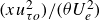 $(xu_{\tau o}^{2})/(\theta U_{e}^{2})$
. Cases with steeper slopes would presumably be farther from equilibrium due to the shorter dimensionless distance available to adjust to rising β. Equilibrium can be assessed using the Clauser shape factor,
$(xu_{\tau o}^{2})/(\theta U_{e}^{2})$
. Cases with steeper slopes would presumably be farther from equilibrium due to the shorter dimensionless distance available to adjust to rising β. Equilibrium can be assessed using the Clauser shape factor, $G=({U_{e}}/u_{\tau })(H-1)/H$
, where H = δ
*
/θ is the shape factor. The variation of G with β is shown for the present cases in figure 8 along with an equilibrium curve from Mellor & Gibson (Reference Mellor and Gibson1966). The results in figures 7 and 8 are consistent. Cases 1 and 5 exhibit the fastest rise in β with dimensionless streamwise distance and have the lowest G values below the equilibrium curve. This is consistent with case 1 having lower values than case 8 in figure 6. It is also consistent with the closer agreement of cases 4 and 8 in figure 6, since both of these cases have a slower rise of β than in case 1, and both are closer to equilibrium, as shown in figure 8.
$G=({U_{e}}/u_{\tau })(H-1)/H$
, where H = δ
*
/θ is the shape factor. The variation of G with β is shown for the present cases in figure 8 along with an equilibrium curve from Mellor & Gibson (Reference Mellor and Gibson1966). The results in figures 7 and 8 are consistent. Cases 1 and 5 exhibit the fastest rise in β with dimensionless streamwise distance and have the lowest G values below the equilibrium curve. This is consistent with case 1 having lower values than case 8 in figure 6. It is also consistent with the closer agreement of cases 4 and 8 in figure 6, since both of these cases have a slower rise of β than in case 1, and both are closer to equilibrium, as shown in figure 8.
Clauser pressure gradient parameter vs dimensionless streamwise position. Legend indicates case number.

Clauser shape factor vs β. Legend indicates case number, equilibrium black line from Mellor & Gibson (Reference Mellor and Gibson1966).

Physically, the departure from equilibrium shown in 8 can be explained in terms of the response of the boundary layer to the forces acting on it. As the pressure gradient changes, the pressure forces acting on the boundary layer change, by definition. This results in an immediate change in β. The boundary layer, however, contains mass and momentum, so it cannot respond instantaneously to a suddenly imposed pressure force. In the case of an increasing β, some time is needed for the boundary layer flow to decelerate toward a new equilibrium as the increasing APG imposes a force that is opposed to the streamwise flow direction. During this interval, as the boundary layer decelerates, the shape of the velocity profile will gradually adjust, the mean velocity deficit will increase, and the skin friction coefficient will decrease due to the increasing velocity deficit in the near-wall region. As the boundary layer profile adjusts, G will increase due to the increase in H (δ * will increase as the velocity deficit increases, while the rate of increase in the momentum deficit, expressed as θ, will be lessened due to the decreasing skin friction) and decreasing u τ . The change in G will therefore lag the change in β during a period of non-equilibrium. If β is changing rapidly, a greater lag in the response of G and greater departure from equilibrium can be expected. The rate at which the boundary layer can adjust will depend on both the forces (pressure and skin friction) acting directly on the boundary layer with the subsequent response of the momentum, and the transport of momentum within the boundary layer due to turbulent mixing. The scaling used in (3.1) attempts to quantify these effects, so that a steeper slope in figure 7 should correspond to a greater departure from equilibrium. For most of the cases in figure 8, the agreement with the equilibrium curve indicates that the rate of change of β shown in figure 7 was sufficiently slow so that the boundary layer, at least in terms of the mean velocity, remained in a near equilibrium condition.
Turbulence quantities, such as the Reynolds stresses shown in figures 5 and 6, do not respond directly to the pressure forces acting on the boundary layer, but only indirectly via the mean velocity changes. The primary production terms for the Reynolds stresses are proportional to the mean velocity gradient in the wall-normal direction. Hence, changes in the Reynolds stresses will lag changes in the mean velocity, which in turn will lag changes in the pressure gradient. This suggests that the turbulence quantities should be more sensitive to departure from equilibrium than the mean velocity and therefore more visibly dependent on the β history.
To directly compare the profiles from all cases, a y/δ location from the middle of the profile is chosen, and the value of each profile at this location is shown in figure 9. The Reynolds normal stresses are not shown as they have the same qualitative behaviour as the Reynolds shear stress. The location y/δ = 0.5 is used, but the results are qualitatively the same using any y/δ between 0.2 and 0.8. Although a single point does not indicate the shape of the full profile, it does indicate the departure from the ZPG profile and allows the comparison of all profiles from all cases in a single plot as a function of β. The data for the mean velocity defect and the Reynolds shear stress collapse for most cases. This may indicate that these cases have β increasing at a slow enough rate that they are near equilibrium, which is consistent with the Clauser shape factor results of figure 8. It implies that for these cases the particular upstream β history may not be as important. Cases 1 and 5 are exceptions, with values below the other cases at all β. Again, this is consistent with the lower G values in figure 8 for these cases and the faster rise of β in figure 7. Case 9 has the slowest increase of β in figure 7 of any case reaching β >2, suggesting that this case may be closest to equilibrium. In agreement, the profile values for case 9 lie slightly above the other cases in figure 9(b), particularly at the downstream stations, as was also observed for the turbulence quantities in figure 5. Note that some caution is helpful when evaluating differences between cases. In figure 9(b), for example, the difference between most cases at any given β is of the order 15 %, which is comparable to the uncertainty. Overall trends may have physical significance, but conclusions drawn based on individual data points may not be as meaningful.
Profile values of (a) defect velocity and (b) Reynolds shear stress at y/δ = 0.5 as functions of β. Legend indicates case number.

To compare rough- and smooth-wall cases that appear to depart from equilibrium, figure 10 shows profiles from cases 1 and 5 at locations where β ≈ 6 in each case (β = 6.6 in case 1 and 5.6 in case 5). These cases both have a higher rate of rise of β than the other cases in figure 7. The mean defect profiles agree to within approximately 10 %, which is just within the overlap of the uncertainties for the two cases. The Reynolds stress profiles are approximately 20 % higher for case 5, which is inconsistent with the higher local β and more rapid rise in β for case 5. The agreement in these cases is not perfect, but is still better than the agreement between cases 1 and 8 in figure 6. This suggests that if the β vs dimensionless x history is matched, that similarity between rough- and smooth-wall cases might be achieved even in cases that lag behind equilibrium conditions.
Velocity profiles for cases 1 (blue) and 5 (magenta) where β ≈ 6: (a) mean velocity defect, (b) streamwise Reynolds normal stress, (c) wall-normal Reynolds normal stress, (d) Reynolds shear stress.

Figure 8 indicates that the value of G relative to β is an indicator of equilibrium, which raises the question of whether matching G between cases might result in agreement. Figure 11 shows mean velocity and Reynolds shear stress profiles for cases with G = 9 and G = 20 as examples. The agreement between cases is within approximately 10 % in both the mean velocity and Reynolds shear stress, and includes cases both near and farther from equilibrium (i.e. case 1 at G = 9 and case 5 at G = 20). Figure 12 shows the value of the mean defect velocity and the Reynolds shear stress at y/δ = 0.5 for all cases as a function of G. The agreement between cases is within about 10 % at most locations in the boundary layer with larger scatter for the Reynolds shear stress.
Velocity profiles for G = 9 (a) mean velocity defect, (b) Reynolds shear stress; and G = 20 (c) mean velocity defect, (d) Reynolds shear stress.

Profile values of (a) defect velocity and (b) Reynolds shear stress at y/δ = 0.5 as functions of G. Legend indicates case number.

3.2. The APG following an FPG
As another test of upstream history effects, cases 11 and 12 for the smooth wall and case 13 for the rough wall had an initial ZPG of length 0.6 m with an FPG of length 0.5 m downstream of the ZPG, and the APG region of interest immediately downstream of the ZPG, as shown in figure 1(c). As in the previous section, the origin for x is taken at the start of the APG. Cases 4 and 9 from above with a change from a ZPG to an APG are used as comparison cases. Figure 13 shows the free-stream velocity distribution, and figure 14 shows the β history as a function of x and dimensionless x. Figure 15 shows G vs β in the format of figure 8. All cases appear to be near equilibrium except for the downstream stations of cases 11 and 12, where a change in the rate of β increase results in G above the equilibrium curve.
Free-stream velocity normalised on free-stream velocity at start of APG. Legend indicates case number.

Clauser pressure gradient parameter vs (a) dimensional streamwise position, (b) dimensionless streamwise position. Legend indicates case number.

Clauser shape factor vs β. Legend indicates case number, equilibrium black line from Mellor & Gibson (Reference Mellor and Gibson1966).

Figure 16 shows a comparison of profiles from smooth-wall cases 4 and 11 at similar β. At the first station there is a clear difference between the cases since case 11 is at the end of an FPG, resulting in a lower velocity deficit and turbulence, while case 4 is in a canonical ZPG state. Downstream, however, the two cases come into better agreement. This indicates that the upstream condition has an initial important effect, but that this is quickly overwhelmed by the effect of the APG. Note that all the profiles shown are from stations upstream of the departure of case 11 from the equilibrium curve in figure 15. Figure 17 shows a comparison of cases 4 and 12. Similar to figure 16, there is a difference at the most upstream station which becomes smaller at the downstream stations for the mean velocity. There are clear differences in the Reynolds shear stress, with case 12 actually rising above case 4 at the downstream stations. The downstream stations correspond to G rising above the equilibrium curve in figure 8. It again appears that the upstream FPG has an initial effect on the boundary layer, but its significance decreases quickly as the APG progresses. A change in the rate of β increase, however, can result in differences between cases by causing a departure from equilibrium. When evaluating scaling and similarity, at least in the region near a change in pressure gradient, it is important that the upstream pressure gradient history be similar between the cases being compared. An upstream canonical (ZPG) condition for both cases would achieve this.
Velocity profiles for cases 4 (black) and 11 (red): (a) mean velocity defect, (b) streamwise Reynolds normal stress, (c) wall-normal Reynolds normal stress, (d) Reynolds shear stress. Legend indicates successive streamwise locations with matching and increasing β for all cases.

Velocity profiles for cases 4 (black) and 12 (magenta): (a) mean velocity defect, (b) streamwise Reynolds normal stress, (c) wall-normal Reynolds normal stress, (d) Reynolds shear stress. Legend indicates successive streamwise locations with matching and increasing β for all cases.

Figure 18 shows a comparison between rough-wall Cases 9 and 13. As in the smooth-wall cases, there is a difference between the profiles at the first station due to the difference between the ZPG and FPG upstream state, but the agreement becomes closer as the flow moves downstream. Differences at the last two stations may be attributable to β not being exactly the same for the two cases.
Velocity profiles for cases 9 (red) and 13 (blue): (a) mean velocity defect, (b) streamwise Reynolds normal stress, (c) wall-normal Reynolds normal stress, (d) Reynolds shear stress. Legend indicates successive streamwise locations with matching and increasing β for all cases.

Figure 18 Long description
The image contains four separate line graphs labeled (a), (b), (c), and (d), each depicting different velocity profiles for cases 9 (red) and 13 (blue). Panel A: The graph shows the mean velocity defect. The x-axis is labeled y/delta and the y-axis is labeled (Ue-U)/utau. The legend indicates successive streamwise locations with matching and increasing values for all cases. Panel B: The graph shows the streamwise Reynolds normal stress. The x-axis is labeled y/delta and the y-axis is labeled u^2/u^2_tau. The legend indicates successive streamwise locations with matching and increasing values for all cases. Panel C: The graph shows the wall-normal Reynolds normal stress. The x-axis is labeled y/delta and the y-axis is labeled v^2/u^2_tau. The legend indicates successive streamwise locations with matching and increasing values for all cases. Panel D: The graph shows the Reynolds shear stress. The x-axis is labeled y/delta and the y-axis is labeled -uv/u^2_tau. The legend indicates successive streamwise locations with matching and increasing values for all cases.
3.3. Case approaching separation
Rough-wall case 13, considered in the previous section, had a rapidly growing boundary layer and β. It is considered in more detail next, including the downstream stations not shown above, to show the nature of a rough-wall boundary layer approaching separation. Figure 19 shows the streamwise increase of β, and figure 20 shows G vs β. Note that the ranges of β and G in these figures are an order of magnitude larger than in the other cases shown in figure 8 and 15. Although β becomes very large, the case remains close to the equilibrium curve in figure 20. The momentum thickness Reynolds number, Re θ = U e θ/ν, increases nearly linearly with x from 2600 to 14,200. The friction Reynolds number, Re τ = u τ δ/ν, drops nearly linearly from 1900 to 800. The shape factor, H = δ * /θ, increases nearly linearly from 1.6 to 2.9. The large H is an indicator that the boundary layer is approaching separation. The roughness Reynolds number, k s + = u τ k s /ν, drops nearly linearly from 290 at the first station to 60 at the sixth station, followed by a more gradual drop to 21 at the last station. These k s + values indicate fully rough conditions upstream and transitionally rough at the last few stations. Note that as a boundary layer approaches separation, it cannot remain hydrodynamically fully rough due to u τ approaching zero.
Clauser pressure gradient parameter for case 13 vs (a) dimensional streamwise position, (b) dimensionless streamwise position.

Clauser shape factor vs β. Equilibrium black line from Mellor & Gibson (Reference Mellor and Gibson1966).

Figure 21 shows the mean velocity and Reynolds stresses for all stations of this case. The velocity deficit becomes very large, indicating an approach to separation. The boundary layer did not actually separate because the boundary layers on the test wall and upper wall of the test section merged slightly downstream of the last measurement station shown. Much of the change in figure 21 is due to the decrease in the friction velocity. If the wake region scaling proposed by Volino & Schultz (Reference Volino and Schultz2025a ) is used, in which the distance from the wall is shifted by the displacement thickness, y * = (y – δ *)/(δ – δ *), and the velocities are all normalised using the same upstream friction velocity (for the present case u τo = 0.128 m/s found between stations 1 and 2), the results are as shown in figure 22. After an initial transient associated with the upstream FPG, the profiles collapse in the outer region. This is associated with a detachment of the turbulent eddies from the wall in the APG and a subsequent loss of scaling with the local friction velocity. The use of an upstream velocity to collapse the profiles in an APG boundary layer was also used by Aubertine & Eaton (Reference Aubertine and Eaton2005), who used U e at the start of an APG to collapse the results acquired at downstream stations.
Velocity profiles for case 13: (a) mean velocity defect, (b) streamwise Reynolds normal stress, (c) wall-normal Reynolds normal stress, (d) Reynolds shear stress. Legend indicates streamwise station.

Velocity profiles for case 13 in outer coordinates of Volino & Schultz (Reference Volino and Schultz2025a ): (a) mean velocity defect, (b) streamwise Reynolds normal stress, (c) wall-normal Reynolds normal stress, (d) Reynolds shear stress. Legend indicates streamwise station.

The present use of u τ is similar, but allows for the inclusion of both rough- and smooth-wall data. More details on this scaling are provided in Volino & Schultz (Reference Volino and Schultz2025a ).
The third-order moments of the turbulence provide information on the transport of the Reynolds stresses and how the transport is affected by the APG. Figure 23 shows profiles of the skewness of the u′
and v′
fluctuating velocity. At the first station, which is at the end of the FPG region, the u′
skewness is positive everywhere with a peak in the centre of the boundary layer, and the v′
skewness is similar but with opposite sign. As described in Volino & Schultz (Reference Volino and Schultz2025b
), an FPG suppresses the turbulence in the outer part of the boundary layer, thus reducing the effect of sweep motions of high speed (u′
>0) fluid moving toward the wall (v′
<0). What remains are ejections of low speed (u′
<0) fluid moving away (v′
>0) from the near-wall region. The ejections produce the skewness results seen at station 1. As the flow moves downstream in the APG, the turbulence in the near-wall region drops, as shown in figure 21, due to the drop in mean shear, and the peaks in the Reynolds stresses move outward to approximately y/δ = 0.6. The transport of the fluctuations towards the wall results in positive u′
and negative v′
inside of y/δ = 0.6, and the opposite signs farther from the wall. Downstream of the sixth station, there is little change in the skewness profiles as the boundary layer moves toward separation. Figure 24 provides another view of the transport, showing profiles of $\overline{u'^{2}v'}$
, which can be associated with the wall-normal transport of
$\overline{u'^{2}v'}$
, which can be associated with the wall-normal transport of $\overline{u'^{2}}$
. If the local friction velocity is used to normalise the profiles, the profile peaks become very large at the downstream stations due to the decrease in u
τ
. To allow the profiles at all stations to be visible in the plot simultaneously, u
τo
at the start of the APG is used for normalising. At the first station, there is a positive peak at y/δ = 0.2. As with the skewness in figure 23(a), this peak can be associated with ejections of near-wall fluid in the FPG region. This peak moves outward in the APG as the Reynolds stress peaks move to the outer part of the boundary layer. As the
$\overline{u'^{2}}$
. If the local friction velocity is used to normalise the profiles, the profile peaks become very large at the downstream stations due to the decrease in u
τ
. To allow the profiles at all stations to be visible in the plot simultaneously, u
τo
at the start of the APG is used for normalising. At the first station, there is a positive peak at y/δ = 0.2. As with the skewness in figure 23(a), this peak can be associated with ejections of near-wall fluid in the FPG region. This peak moves outward in the APG as the Reynolds stress peaks move to the outer part of the boundary layer. As the $\overline{u'^{2}}$
peak moves outward, sweeps originating from it cause a negative
$\overline{u'^{2}}$
peak moves outward, sweeps originating from it cause a negative $\overline{u'^{2}v'}$
peak to emerge at y/δ = 0.2.
$\overline{u'^{2}v'}$
peak to emerge at y/δ = 0.2.
Skewness profiles for case 13: (a) u′ component, (b) v′ component. Legend indicates streamwise station.


Profiles of the primary production terms for $\overline{u'^{2}}$
and
$\overline{u'^{2}}$
and $\overline{u'v'}$
are shown in figure 25. At the upstream station there is a near-wall peak that drops to zero in the outer half of the boundary layer due to the effect of the FPG in straining and suppressing the turbulence in the outer region, as discussed in Volino & Schultz (Reference Volino and Schultz2025b
). As the flow moves downstream in the APG, the production peak shifts outward, and the near-wall production drops toward zero. As the boundary layer moves toward separation, the turbulence generated upstream remains in the outer region, but near-wall production, which would cause the turbulence to grow, is suppressed due to the decreasing velocity gradient near the wall. The drop in near-wall velocity caused by the APG results in a larger mean velocity deficit and less turbulent mixing in the inner region, which lead to eventual separation.
$\overline{u'v'}$
are shown in figure 25. At the upstream station there is a near-wall peak that drops to zero in the outer half of the boundary layer due to the effect of the FPG in straining and suppressing the turbulence in the outer region, as discussed in Volino & Schultz (Reference Volino and Schultz2025b
). As the flow moves downstream in the APG, the production peak shifts outward, and the near-wall production drops toward zero. As the boundary layer moves toward separation, the turbulence generated upstream remains in the outer region, but near-wall production, which would cause the turbulence to grow, is suppressed due to the decreasing velocity gradient near the wall. The drop in near-wall velocity caused by the APG results in a larger mean velocity deficit and less turbulent mixing in the inner region, which lead to eventual separation.
Profiles of primary productions terms for case 13: (a) $\overline{u'^{2}}$
production, (b)
$\overline{u'^{2}}$
production, (b) $\overline{u'v'}$
production. Legend indicates streamwise station.
$\overline{u'v'}$
production. Legend indicates streamwise station.

Profiles of ratio of contributions to $\overline{u'v'}$
from Q2 and Q4. Legend as in figure 25.
$\overline{u'v'}$
from Q2 and Q4. Legend as in figure 25.

To further illustrate the change induced by the APG, quadrant analysis, as describe by Willmarth & Lu (Reference Willmarth and Lu1972) and Wallace, Eckelmann & Brodkey (Reference Wallace, Eckelmann and Brodkey1972), can be used to determine the relative importance of different flow structures. The instantaneous velocity signal is categorised based on the signs of u′
and v′
. Quadrants 2 (Q2, ejections, u′
<0, v′
>0) and 4 (Q4, sweeps, u′
>0, v′
<0) are dominant in turbulent boundary layers and contribute to negative $\overline{u'v'}$
. Figure 26 shows profiles of the ratio of the contributions from Q2 and Q4. In canonical ZPG boundary layers, the value rises from the wall to a local peak of approximately 1.4 at y/δ = 0.07, then drops to a local minimum of approximately 1.2 at y/δ = 0.3, before rising to 2 at the edge of the boundary layer. The FPG at station 1 suppresses the turbulence in the outer part of the boundary layer, which reduces the effect of the sweeps moving closer to wall and raises the Q2/Q4 ratio. The APG has the opposite effect. The reduced turbulence production, shown in figure 25, results in less effective ejections, while the turbulence in the outer region remains and continues to produce sweeps. The result is a low Q2/Q4 ratio, particularly near the wall where the value drops to approximately 0.8. The present observations are consistent with those of Skåre & Krogstad (1994) and Deshpande & Vinuesa (2024), who also considered APG boundary layers. The profiles show no change over the last five stations. Although the boundary layer is not in equilibrium, as evidenced by the growing velocity deficit in figure 21, it appears that it has in some sense reached an asymptotic condition that will eventually lead to separation if allowed to continue.
$\overline{u'v'}$
. Figure 26 shows profiles of the ratio of the contributions from Q2 and Q4. In canonical ZPG boundary layers, the value rises from the wall to a local peak of approximately 1.4 at y/δ = 0.07, then drops to a local minimum of approximately 1.2 at y/δ = 0.3, before rising to 2 at the edge of the boundary layer. The FPG at station 1 suppresses the turbulence in the outer part of the boundary layer, which reduces the effect of the sweeps moving closer to wall and raises the Q2/Q4 ratio. The APG has the opposite effect. The reduced turbulence production, shown in figure 25, results in less effective ejections, while the turbulence in the outer region remains and continues to produce sweeps. The result is a low Q2/Q4 ratio, particularly near the wall where the value drops to approximately 0.8. The present observations are consistent with those of Skåre & Krogstad (1994) and Deshpande & Vinuesa (2024), who also considered APG boundary layers. The profiles show no change over the last five stations. Although the boundary layer is not in equilibrium, as evidenced by the growing velocity deficit in figure 21, it appears that it has in some sense reached an asymptotic condition that will eventually lead to separation if allowed to continue.
The change in flow structure caused by the APG is shown with the R
uu
correlation in the x–y plane in figure 27. The streamwise extent of the R
uu
contours decreases as the flow moves through the APG and the inclination angle of the structure, found by fitting a line through the major axis of the contours, increases from approximately 15 $^{\circ}$
to about 22
$^{\circ}$
to about 22 $^{\circ}$
. For the example shown, the correlation is centred at y/δ = 0.4, but behaviour is similar if other wall-normal distances are used. The APG is effectively a force pushing upstream against the flow direction on the turbulent structures in the boundary layer (e.g. the hairpin packets that produce the correlation of figure 27), thereby compressing the structures in the streamwise direction relative to δ and rotating the structures to a higher inclination angle relative to the wall.
$^{\circ}$
. For the example shown, the correlation is centred at y/δ = 0.4, but behaviour is similar if other wall-normal distances are used. The APG is effectively a force pushing upstream against the flow direction on the turbulent structures in the boundary layer (e.g. the hairpin packets that produce the correlation of figure 27), thereby compressing the structures in the streamwise direction relative to δ and rotating the structures to a higher inclination angle relative to the wall.
Contours of R uu in x–y plane centred at y/δ = 0.4 for stations (a) b, (b) e, (c) h, (d) j of case 13. Contour spacing 0.1. R uu = 1 at centre of correlation.

Figure 28 shows the R uu correlation in the x–z plane. Again, the APG causes the streamwise extent of the correlation as a fraction of the boundary layer thickness to decrease. The decrease is quantified in figure 29, which shows a cut through the contours along their spanwise centreline. The streamwise extent of the contours is nearly the same at y/δ = 0.15, and at y/δ = 0.4. The APG causes the structures to shrink relative to the local δ. There is little change between the last two streamwise stations shown, in agreement with the quadrant results of figure 26 and the view in figure 27.
Contours of R uu in x–z plane at y/δ = 0.4 for stations (a) b, (b) e, (c) h, (d) j of case 13. Contour spacing 0.1. R uu = 1 at centre of correlation.

Streamwise slices through self-correlation point of R uu : (a) y/δ = 0.15, (b) y/δ = 0.4. Legend indicates streamwise station.

The R uw correlation in the x-z plane is shown in figure 30. The shapes formed by the contours are consistent with the signs of the velocity components associated with rotation of the legs of a hairpin vortex, as explained in Volino & Schultz (Reference Volino and Schultz2023). The symmetry of the pattern, as explained by Ganapathisubramani, Longmire & Marusic (2005), depends on the inclination of the hairpin vortices. A vertical vortex would produce a symmetric pattern, while a vortex inclined in the streamwise direction would produce contours extended in the streamwise direction. At y/δ = 0.15, the streamwise extent of the contours decreases as the APG progresses, consistent with the increased inclination of the structures shown in figure 27. Another change, however, is an increased asymmetry between the upstream and downstream lobes. The upstream lobes become weaker. Since the vortices are inclined relative to the wall and the upstream side is closer to the wall, the weaker correlation could be associated with weaker turbulence in the near-wall region caused by the APG. The contours at the last two streamwise stations are nearly the same, in agreement with the lack of change in other quantities in the downstream region of the APG. At y/δ = 0.4 the streamwise extent of the contours again decreases in the APG, the more vertical vortices result in more symmetry at this distance from the wall, and there is again little change between the two most downstream stations.
Contours of R
uw
in x-z plane at y/δ = 0.4 for stations (a) b, (b) e, (c) h, (d) j of case 13. Contour levels from $-$
0.2 to 0.2 with 0.04 spacing.
$-$
0.2 to 0.2 with 0.04 spacing.

3.4. The ZPG following APG
The cases presented above all had β increasing in an APG. Cases 14 and 15, for the smooth and rough wall, respectively, had an initial FPG of 0.4 m length upstream of an APG of length 0.5 m, and a ZPG downstream of the APG. Measurements were made in the APG and ZPG regions. The two cases had approximately the same β at the end of the APG, as shown in figure 31. As a function of dimensionless streamwise position, shown in figure 31(b), the smooth-wall case had a higher β gradient, but in both cases the rate of increase was low enough that the boundary layer appeared to remain near equilibrium, as shown by G vs β in figure 32. Agreement to within approximately 5 % between the rough- and smooth-wall cases is seen in the mean velocity profiles of figure 33(a). The Reynolds shear stress for the rough-wall case is approximately 15 % higher than for the smooth-wall case in figure 33(b), possibly because the rough-wall case has the lower rate of β increase and is slightly closer to equilibrium. The agreement between the two cases at the end of the APG region suggests that both enter the ZPG region under approximately the same condition.
Clauser pressure gradient parameter vs (a) dimensional streamwise position, (b) dimensionless streamwise position. Legend indicates case number.

Clauser shape factor vs β. Equilibrium black line from Mellor & Gibson (Reference Mellor and Gibson1966). Arrows indicate direction of increasing x.

Velocity profiles for APG region of cases 14 (blue) and 15 (red): (a) mean velocity defect, (b) Reynolds shear stress. Legend indicates successive streamwise locations with matching and increasing β for all cases.

Clauser shape factor vs (a) dimensional streamwise position, (b) dimensionless streamwise position.

Skin friction coefficient, C f /2, (shifted by roughness function in rough-wall case) as function of momentum thickness Reynolds number.

The change from APG to ZPG causes an unavoidable departure from equilibrium. The pressure gradient and β drop almost immediately to zero, but the boundary layer does not return to ZPG conditions as fast. The G value gradually drops, as shown in figures 32 and 34. For the dimensionless $x_{\textit{ZPG}}^{*}$
in figure 34(b), the definition of equation (3.1) is used, but the origin is taken at the start of the ZPG region. The rough-wall case proceeds toward a new equilibrium faster. Figure 35 shows the skin friction coefficient as a function of the momentum thickness Reynolds number. Also shown is a standard correlation for a canonical turbulent boundary layer. In the rough-wall case the skin friction has been shifted by the roughness function
$x_{\textit{ZPG}}^{*}$
in figure 34(b), the definition of equation (3.1) is used, but the origin is taken at the start of the ZPG region. The rough-wall case proceeds toward a new equilibrium faster. Figure 35 shows the skin friction coefficient as a function of the momentum thickness Reynolds number. Also shown is a standard correlation for a canonical turbulent boundary layer. In the rough-wall case the skin friction has been shifted by the roughness function
 \begin{equation}{\unicode[Arial]{x0394}} U^{+}=\frac{1}{\kappa }ln\left(k_{s}^{+}\right)+B-8.5,\end{equation}
with κ = 0.384 and B = 4.2. The k s value used to compute k s + for each profile is set to 2 mm, as determined previously from ZPG cases (Volino & Schultz Reference Volino and Schultz2022). The shift with ΔU + produces equivalency with the smooth-wall case for an equilibrium ZPG flow. In the upstream FPG the skin friction agrees with the correlation. In the APG it drops below the correlation. In the ZPG recovery it rises toward the correlation, but does not quite reach it, at least in the smooth-wall case. Figure 36 shows profiles from the two cases taken at stations with approximately matching G. Canonical ZPG profiles from the direct numerical simulation (DNS) of Sillero, Jiménez & Moser (Reference Sillero, Jiménez and Moser2013), which agree well with both rough- and smooth-wall canonical ZPG experimental data (Volino & Schultz Reference Volino and Schultz2022), are shown for comparison. As with the APG profiles in the previous sections, there is agreement to within the uncertainty in the measurements between the rough- and smooth-wall cases when G is matched. In neither case does the boundary layer reach the ZPG DNS profile in the streamwise distance available in the experiment. The higher defect velocity compared with the DNS agrees with the skin friction coefficient being below the ZPG correlation in figure 35. The Reynolds stresses are much higher in the present cases than in the DNS. The turbulence in the outer part of the boundary layer, which was generated in the upstream FPG and early part of the APG where the mean velocity was higher, remains at a higher value than would be expected for the local value of the friction velocity. Since the friction velocity is not expected to rise much in the ZPG, the only way for turbulence quantities to reach equilibrium ZPG values is through decay, which tends to be a slow process.
Velocity profiles for ZPG region of cases 14 (blue) and 15 (red): (a) mean velocity defect, (b) Reynolds shear stress. Legend indicates successive streamwise locations with matching and decreasing G for all cases. Black line is ZPG DNS of Sillero et al. (Reference Sillero, Jiménez and Moser2013).

Comparing the transition from ZPG to APG with the reverse case, when the boundary layer transitions from a ZPG to an APG, the APG is essentially a force pushing in the upstream direction against the mean flow and the turbulence structures. The pressure gradient forces a change in the mean velocity profile. For the change from an APG to a ZPG, this streamwise pressure force is essentially removed in the ZPG region. One could argue that there is no force directly pushing the mean profile back toward the canonical ZPG condition. Rather, the return to a canonical ZPG state must rely on turbulent transport to redistribute the momentum in the boundary layer. To the extent that turbulent transport represents a slower mechanism for change than a more direct pressure force, the recovery from an APG to a ZPG state will be slower than in the opposite direction, and the boundary layer will be in a non-equilibrium condition during the change.
3.5. Parameters for history effects
It is clear from the results shown that in some cases, β alone is not enough to characterise the state of a boundary layer. If β changes too rapidly, whether by increasing at a high rate in an APG or by dropping to zero at the transition from an APG to a ZPG, the departure from equilibrium can become significant and history effects become important. A parameter that captures history effects could be useful.
Vinuesa et al. (Reference Vinuesa, Örlü, Sanmiguel, Ianiero, Discetti and Schlatter2017) proposed an average β defined as
 \begin{equation}\overline{\beta }=\frac{1}{{\textit{Re}}_{\theta 2}-{\textit{Re}}_{\theta 1}}\int _{{\textit{Re}}_{\theta 1}}^{{\textit{Re}}_{\theta 2}}\beta d{\textit{Re}}_{\theta }.\end{equation}
The starting point for the integration is taken below as the start of the APG, and the ending point is any location downstream. Since the Clauser shape factor was shown above to be useful for describing the boundary layer, it is used in figure 37 to evaluate $\overline{\beta }$
using all of the cases in the present study. For the APG region, the correlation of G to
$\overline{\beta }$
using all of the cases in the present study. For the APG region, the correlation of G to $\overline{\beta }$
is better than the correlation of G to β in some cases, particularly cases 11 and 12 which were shown in figure 15 to depart from equilibrium due to a change in the rate of β increase. The collapse in figure 37(a) is not perfect. Cases 1 and 5, which had the highest gradient of β in figure 7, lie below the other cases. This result is consistent with Gungor, Gungor & Maciel (Reference Gungor, Gungor and Maciel2024) and Mahajan et al. (2025) who also observed that the average β of equation (3.3) cannot account for changes in the boundary layer when β varies rapidly in the streamwise direction. This suggests an additional dependence on the β gradient beyond the averaging done with equation (3.3).
$\overline{\beta }$
is better than the correlation of G to β in some cases, particularly cases 11 and 12 which were shown in figure 15 to depart from equilibrium due to a change in the rate of β increase. The collapse in figure 37(a) is not perfect. Cases 1 and 5, which had the highest gradient of β in figure 7, lie below the other cases. This result is consistent with Gungor, Gungor & Maciel (Reference Gungor, Gungor and Maciel2024) and Mahajan et al. (2025) who also observed that the average β of equation (3.3) cannot account for changes in the boundary layer when β varies rapidly in the streamwise direction. This suggests an additional dependence on the β gradient beyond the averaging done with equation (3.3).
Clauser shape factor as function of average β defined by Vinuesa et al. (Reference Vinuesa, Örlü, Sanmiguel, Ianiero, Discetti and Schlatter2017): (a) APG region of all cases, (b) cases 14 and 15 with change from APG to ZPG. Arrows indicate direction of increasing x.

Figure 37(b) shows G vs $\overline{\beta }$
for cases 14 and 15 with the ZPG region included. There is a hysteresis. The drop in G in the ZPG region is steeper than the rise in the APG. The drop in G with dimensionless x in figure 34(b) suggests an exponential decay of the form
$\overline{\beta }$
for cases 14 and 15 with the ZPG region included. There is a hysteresis. The drop in G in the ZPG region is steeper than the rise in the APG. The drop in G with dimensionless x in figure 34(b) suggests an exponential decay of the form
 \begin{equation}\frac{G-G_{\textit{ZPG}}}{G_{\textit{APG}}-G_{\textit{ZPG}}}=\exp \left(-ax_{\textit{ZPG}}^{*}\right),\end{equation}
where G APG is the value of G at the end of the APG region, and G ZPG is the expected value for a canonical ZPG boundary layer, which is set to 7.1 based on the results in Volino (Reference Volino2020b ) and Volino & Schultz (Reference Volino and Schultz2022). The constant a is set to 80 for the curve shown in figure 34(b). Better fits to the smooth- and rough-wall data are possible using values of a = 60 and a = 100, respectively. Equation (3.4) is simply based on observation of the data. If it does capture the physics, however, it suggests that a ZPG region length of about twice that in the experiment would be needed for the mean velocity profiles to recover to an equilibrium condition. The turbulence quantities would presumably take longer.
4. Conclusions
Velocity profiles were acquired in rough- and smooth-wall boundary layers subject to APGs with β as high as 200. For cases with an APG imposed downstream of a canonical ZPG boundary layer, when β was matched, outer layer similarity between the rough- and smooth-wall profiles of the mean velocity and the Reynolds stresses was observed in many cases. Although β was continuously rising in all cases, indicating that the boundary layer was never in full equilibrium, the Clauser shape factor, G, matched the expectations for equilibrium conditions in most of the cases tested. This suggests that the boundary layers were under near equilibrium conditions. Small differences in β and β history resulted in more visible differences in the turbulence quantities than in the mean velocity.
Deviation from the equilibrium G and differences between cases at the same β were observed in some cases with strong pressure gradients. A dimensionless streamwise coordinate, (xu τo 2 )/(U e 2 θ), was proposed to quantify the rate of increase of β relative to the distance required for the boundary layer to adjust to the changing pressure gradient. When the rate of β increase was large relative to (xu τo 2 )/(U e 2 θ), the mean velocity defect and Reynolds stresses had lower values than in other cases with the same β, indicating that these cases lagged behind the rate of change needed to remain in equilibrium. When cases with the same β vs (xu τo 2 )/(U e 2 θ) were compared, a greater degree of similarity was observed even when the pressure gradient was strong and the cases were not in equilibrium. When profiles from different cases with matching G were compared, similarity was again observed, even when β or its rate of change were different.
The results suggest that if the β history is matched between rough- and smooth-wall cases that outer layer similarity appears to hold in APG boundary layers. If the rate of change of β is moderate, the boundary layer will be in a state near equilibrium, and similarity will hold if β is matched even with differences in the upstream history. The similarity between rough- and smooth-wall boundary layers is an encouraging result for turbulence modelling, which typically presumes that the models developed for smooth-wall boundary layers also apply in rough-wall cases.
Additional cases were considered with an FPG immediately upstream of the APG. The FPG resulted in a lower mean velocity deficit and lower turbulence levels than in a ZPG boundary layer. When the APG was imposed, the effect of the FPG was reversed, and after an initial adjustment the boundary layer became essentially the same as one with a ZPG upstream condition. For a case that approached separation, the boundary layer was never in equilibrium, with β and the velocity deficit continuously increasing, but once adjusted to the APG, the boundary layer structure did not appear to change significantly as the flow moved downstream.
While an APG caused a rapid change in the boundary layer, the reverse process from an APG to a ZPG proceeded more gradually. The high velocity deficit and turbulence levels produced by the APG persisted and appeared to slowly decay toward a canonical ZPG condition. The turbulence quantities in particular remained high for the full length of the measurement region in the experiments. The physical mechanisms most responsible for changes in the velocity and turbulence profiles in non-equilibrium boundary layers for the ZPG to APG case (upstream directed pressure forces) may be different for those in the APG to ZPG case (turbulent transport). The results suggest that a parameter for capturing upstream history, such as an average β, may be useful for particular classes of flows (e.g. a change from a ZPG to an APG), but a single parameter may not be useful for all possible combinations of upstream conditions.
smooth wall, x = 1.60 m at start of APG.

smooth wall, x = 1.60 m at start of APG.

smooth wall, x = 1.60 m at start of APG.

smooth wall, x = 0.80 m at start of APG.

rough wall, x = 1.60 m at start of APG.

rough wall, x = 1.60 m at start of APG.

rough wall, x = 1.60 m at start of APG.

rough wall, x = 0.80 m at start of APG.

rough wall, x = 0.80 m at start of APG.

rough wall, x = 0.80 m at start of APG.

smooth wall, x = 1.106 m at start of APG.

smooth wall, x = 1.106 m at start of APG.

rough wall, x = 1.106 m at start of APG.

smooth wall, x = 0.45 m at start of APG.

rough wall, x = 0.45 m at start of APG.

Acknowledgements
The authors thank the Office of Naval Research for providing financial support under Grant N0001425GI00573. The grant monitors were Dr Y. Lu (Julie) Young and Dr P. Chang. The authors also thank the United States Naval Academy Hydromechanics Laboratory and Project Support Branch for providing technical support.
Disclaimer
The views expressed in this article are those of the authors and do not reflect the official policy or position of the U.S. Naval Academy, the Department of the Navy, the Department of Defense or the U.S. Government.
Declaration of Interests
The authors report no conflict of interest.
Data availability
The LDV data, including profiles of mean velocity and turbulence statistics, as well as boundary layer thicknesses and free-stream and friction velocities are available for all streamwise measurement stations of all cases as an entry in the roughnessdatabase.org maintained at the University of Southampton. The same data are also available on request directly from the authors.
Appendix
Tabulated data with boundary layer parameters are provided here for each streamwise station of each experimental case. Note that x in each table is the distance from the trip. In the figures 1, 3, 4, 7, 13, 14, 19, 31 and 34 above it has been shifted such that x = 0 is at the start of the APG region. The kinematic viscosity, ν, was 1×10⁻⁶ m2/s for all cases.


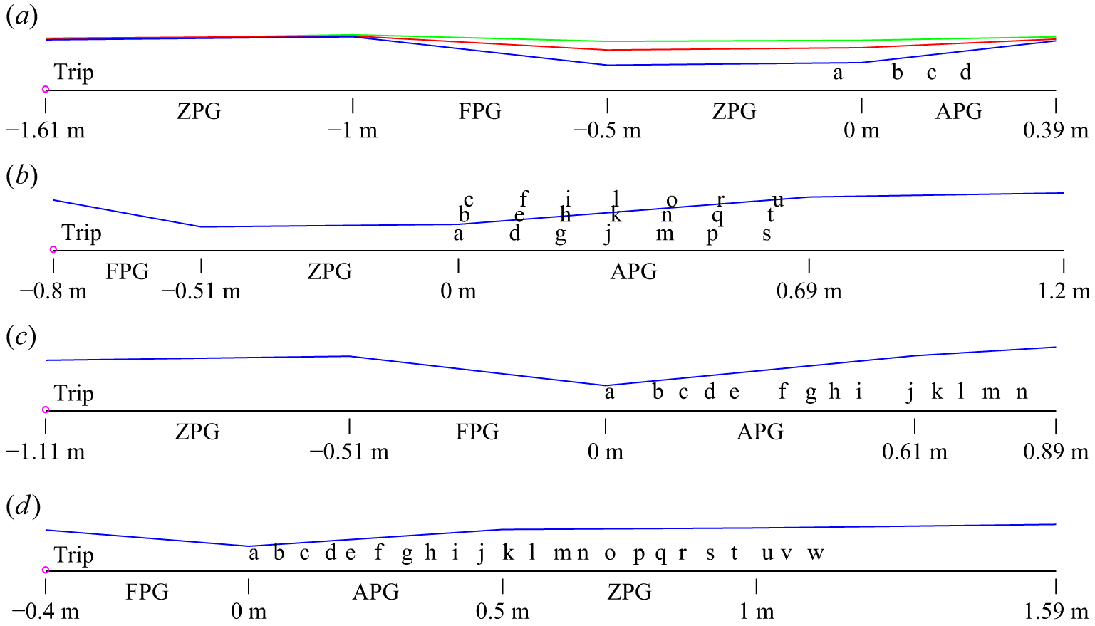
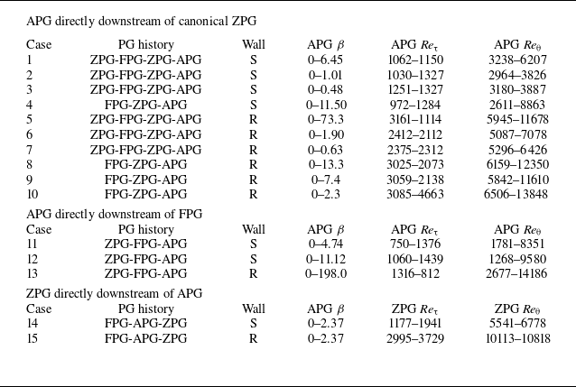


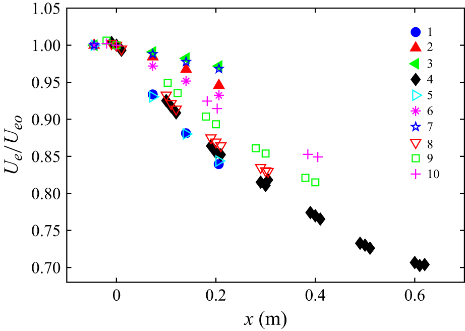
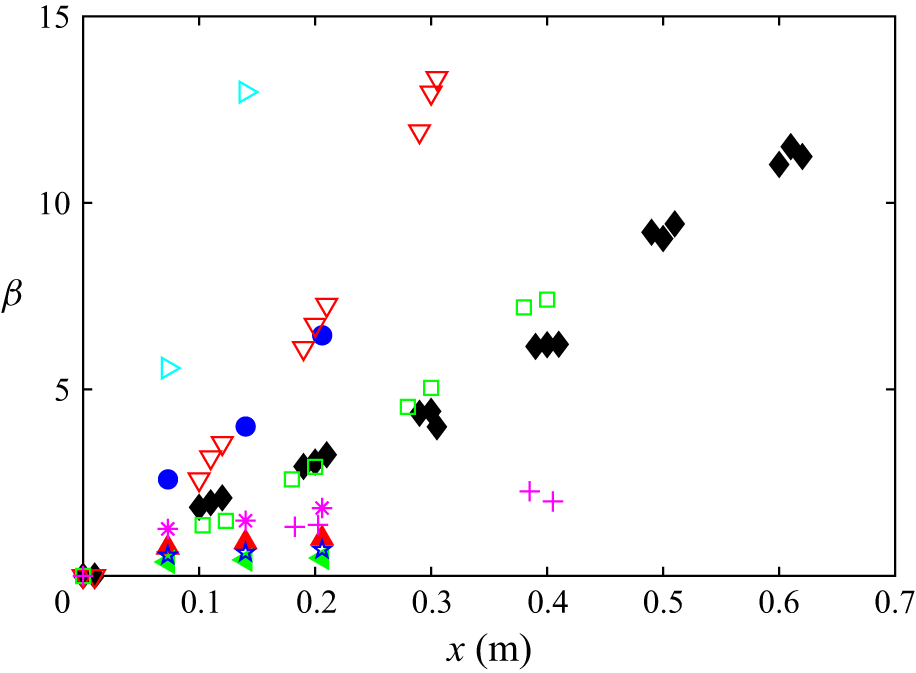
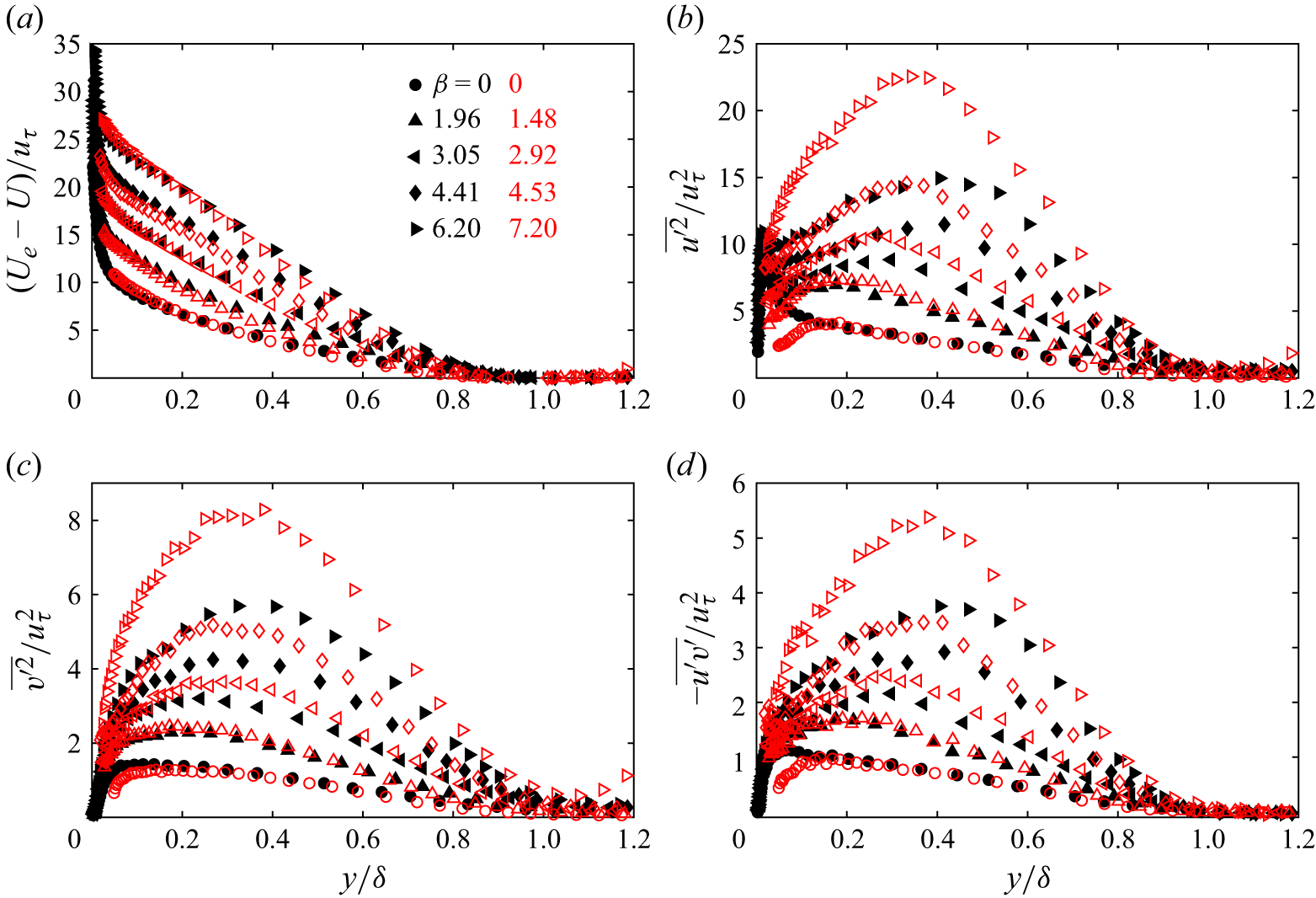
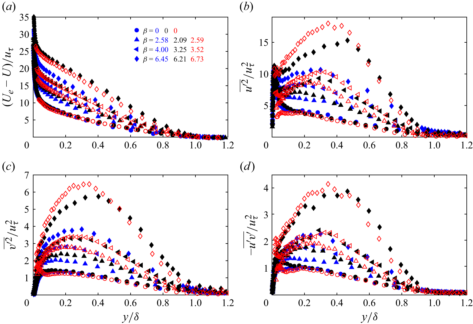
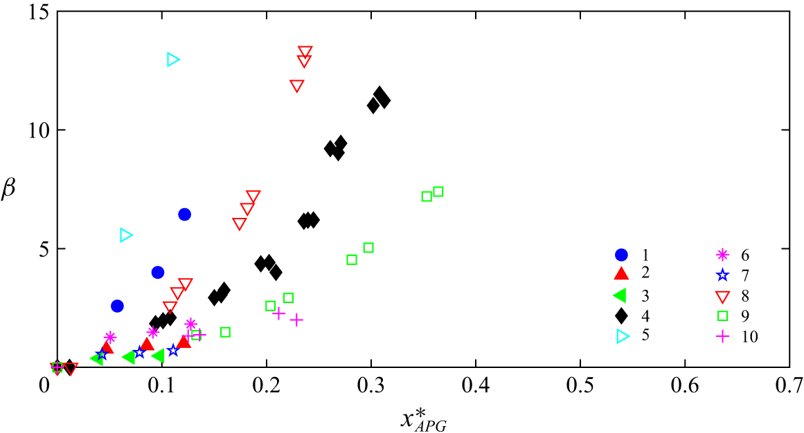
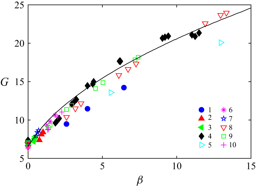
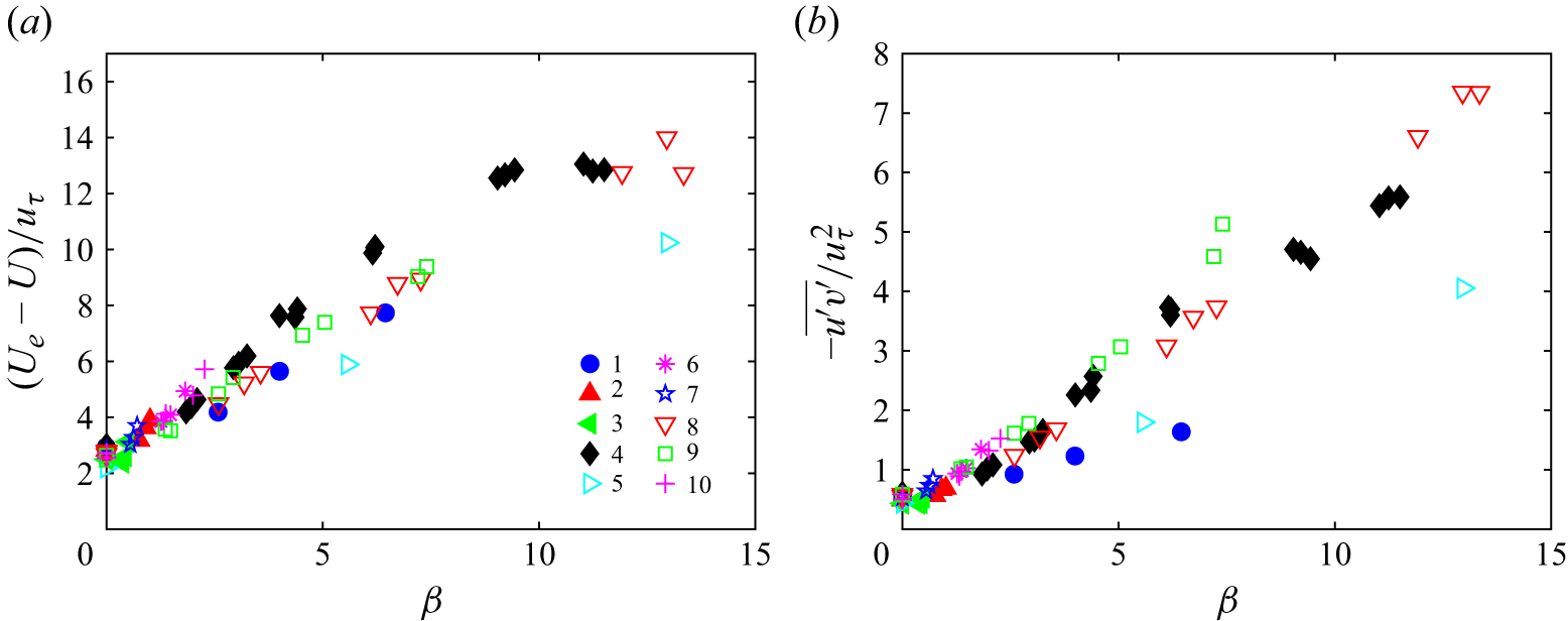
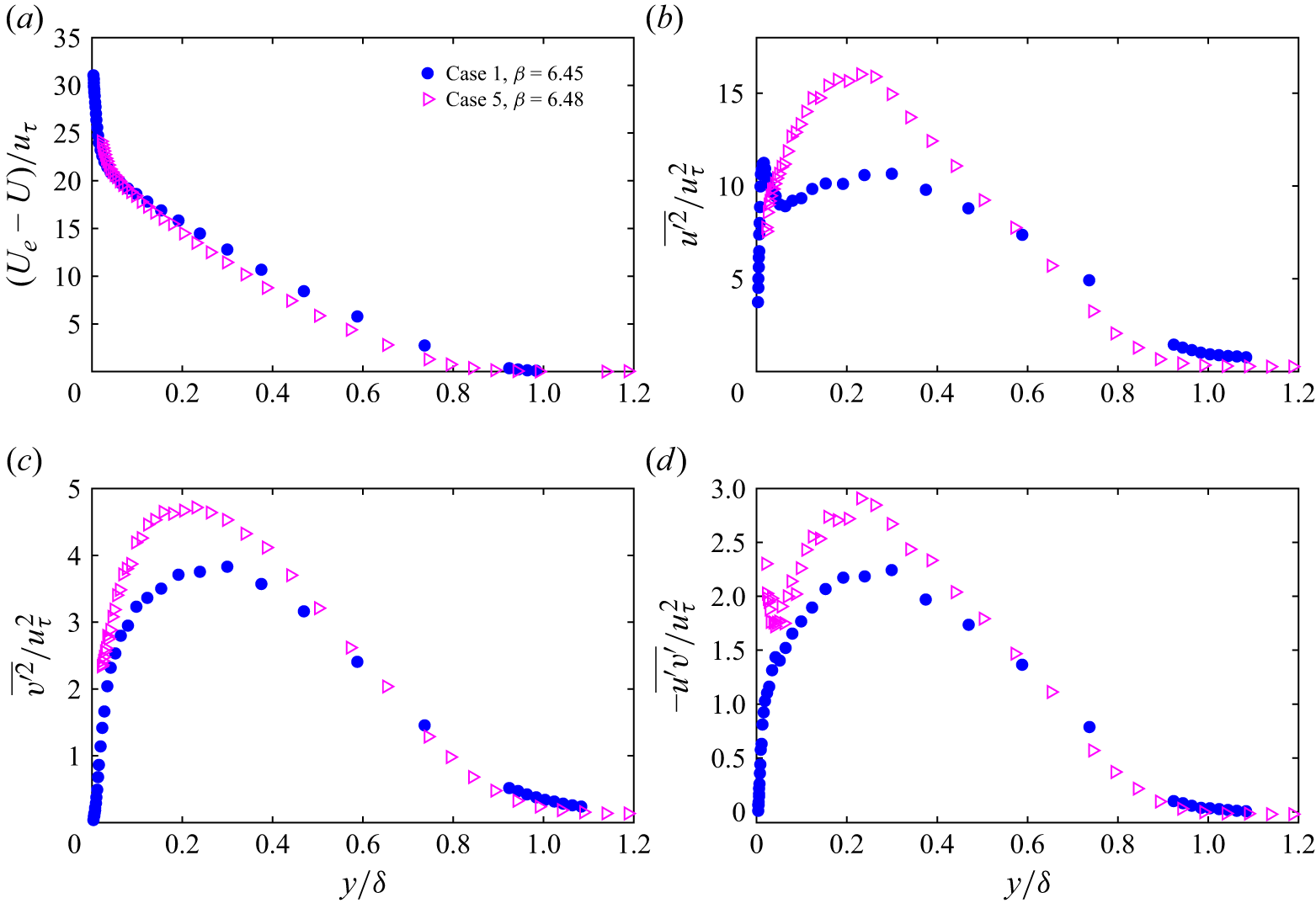
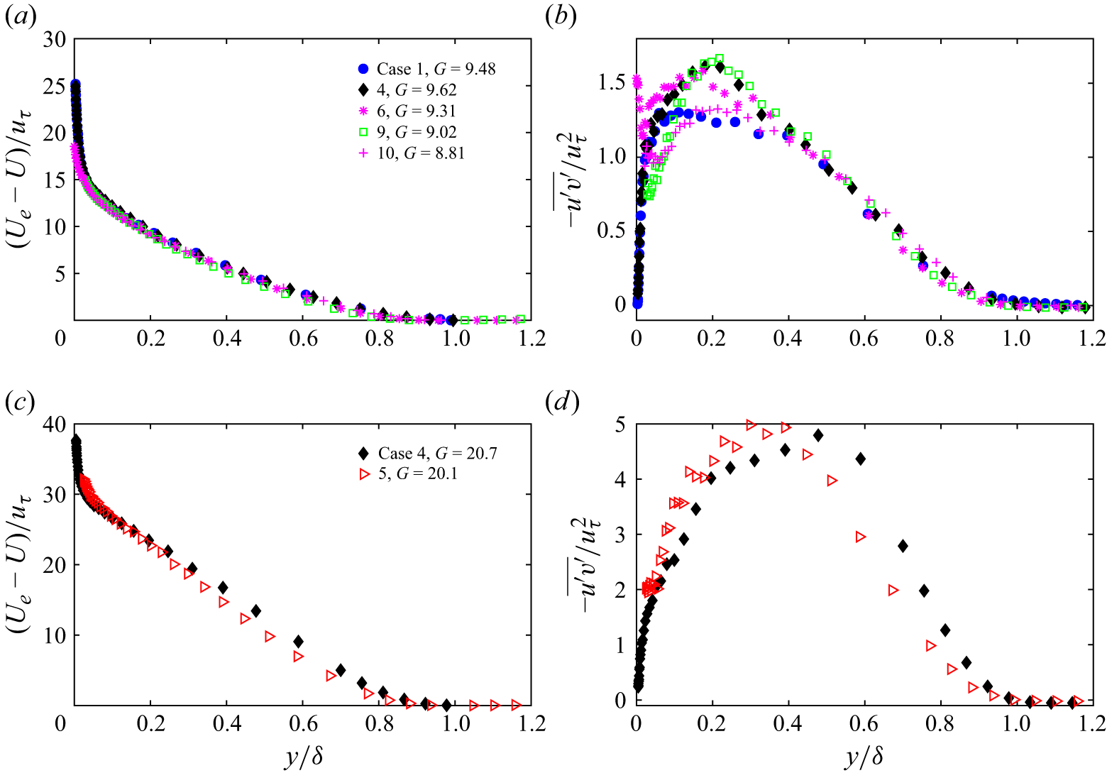
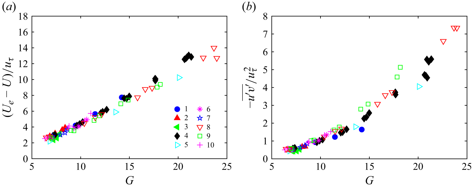
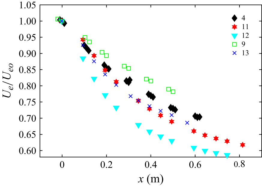
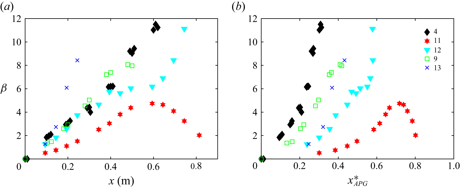
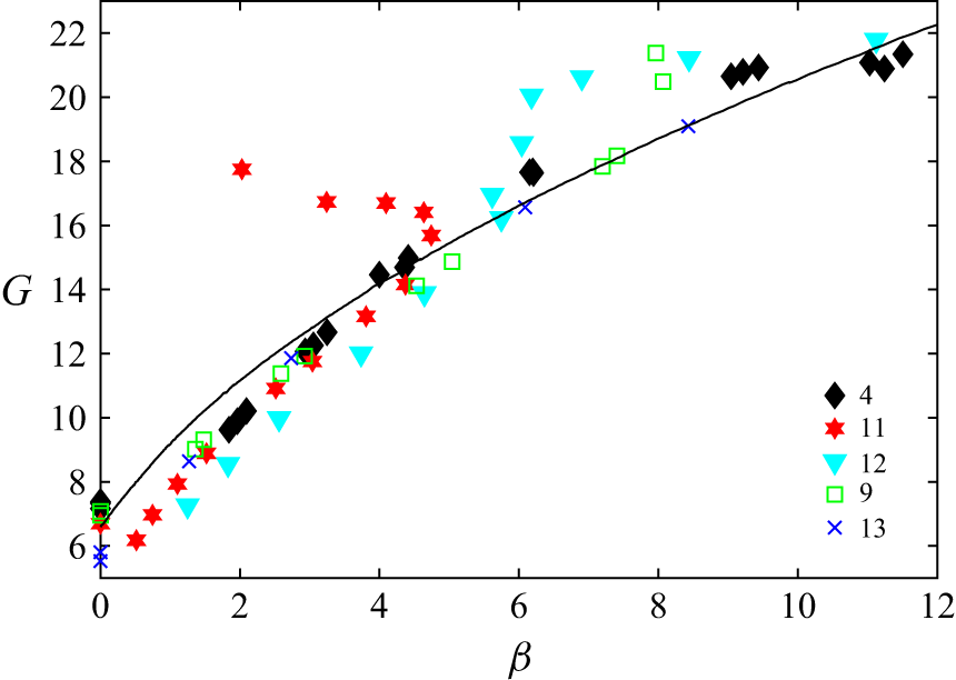
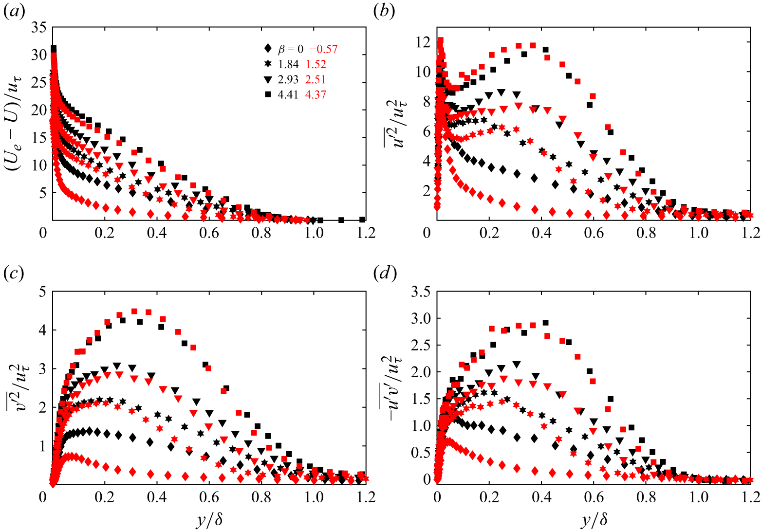
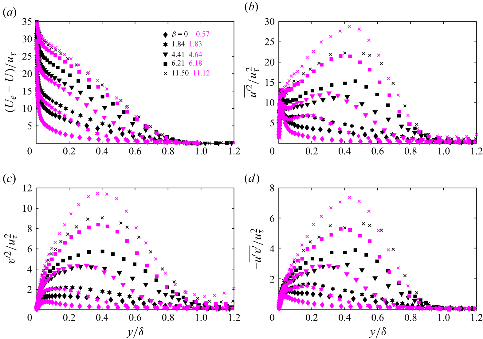
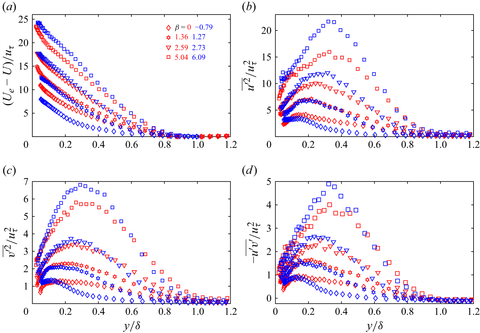
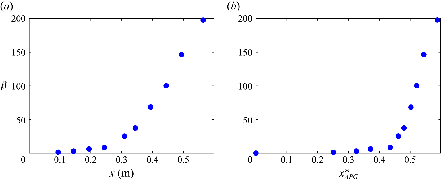
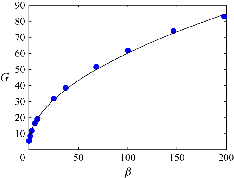
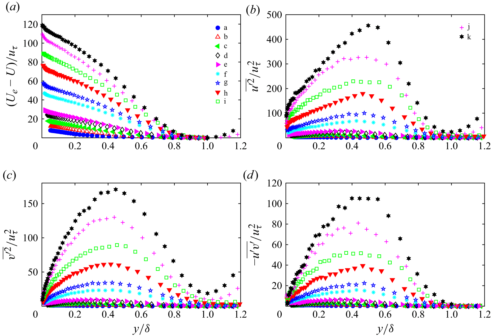
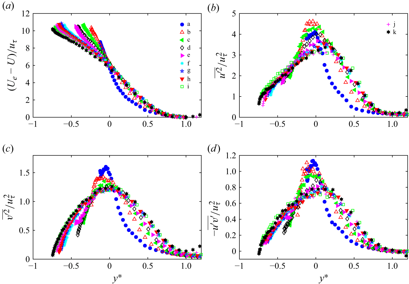
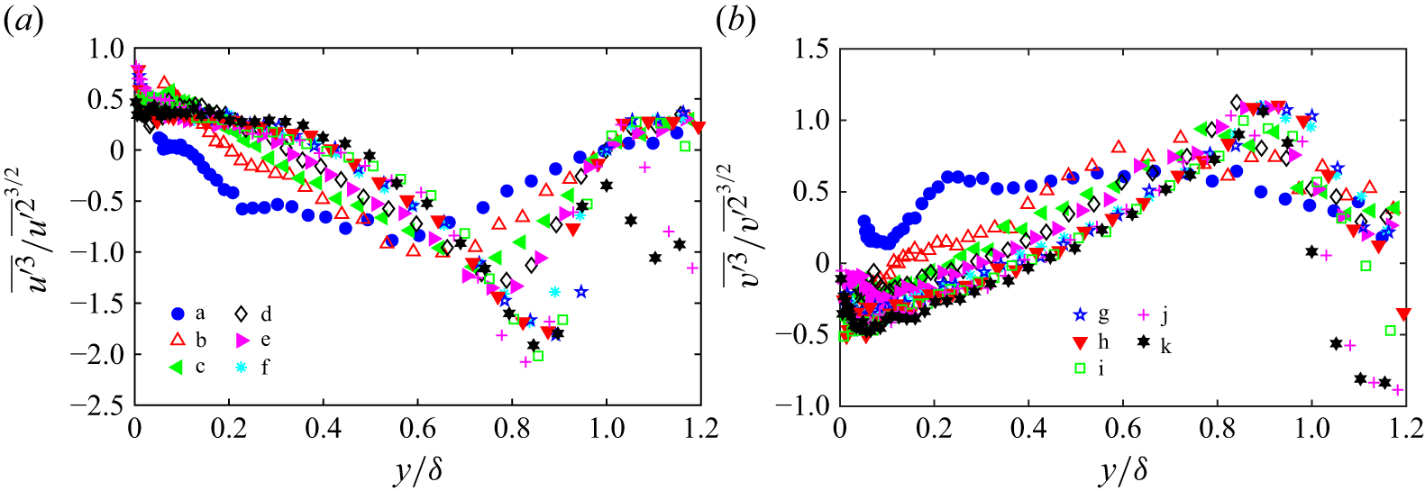
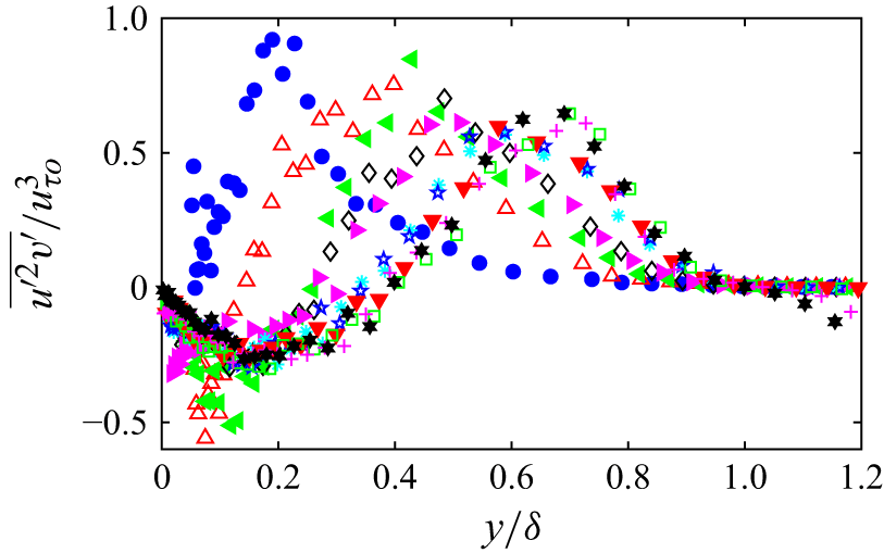
 u′2v′¯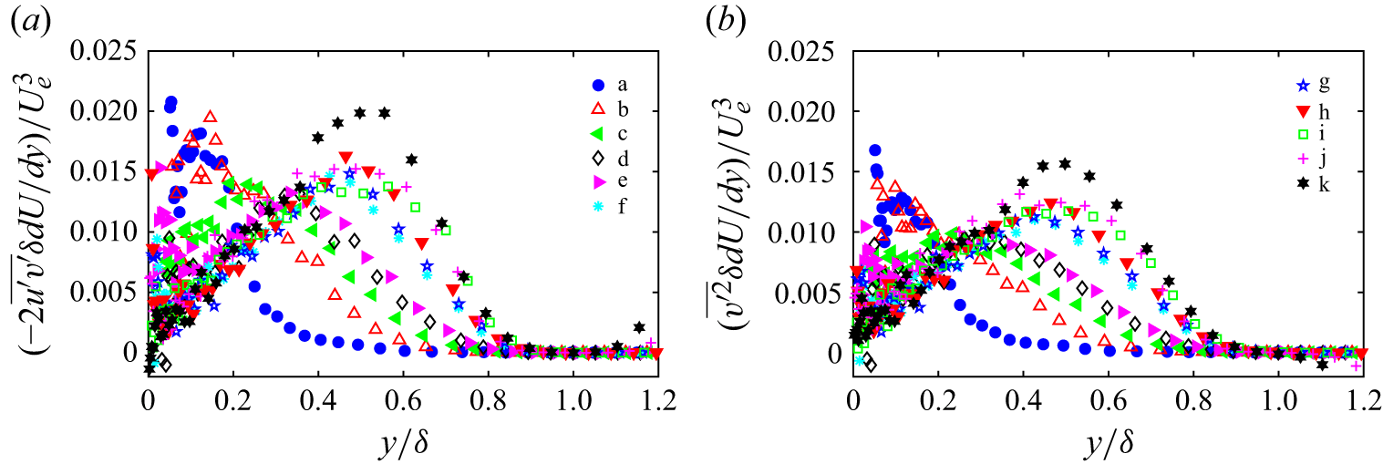
 u′2¯
u′2¯ u′v′¯
u′v′¯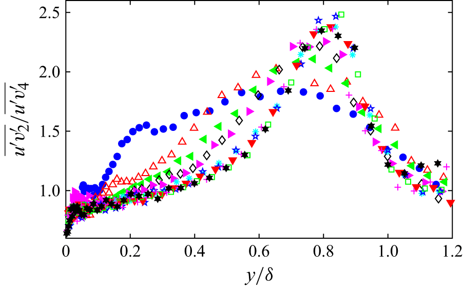
 u′v′¯
u′v′¯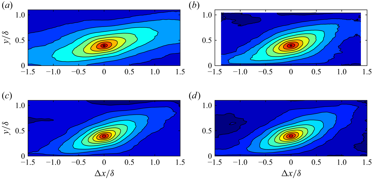
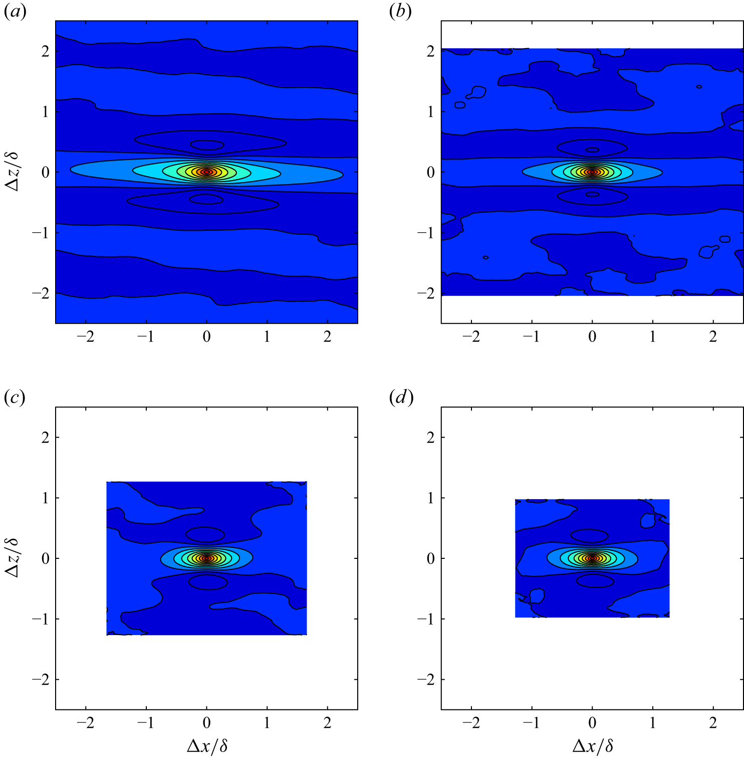
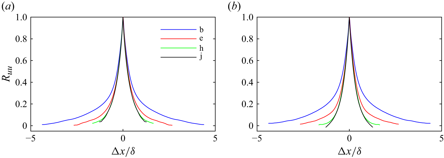
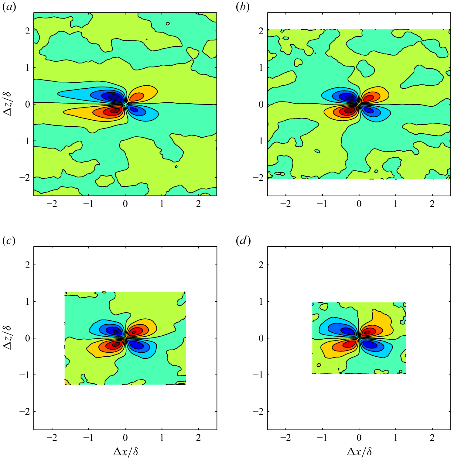
 −
−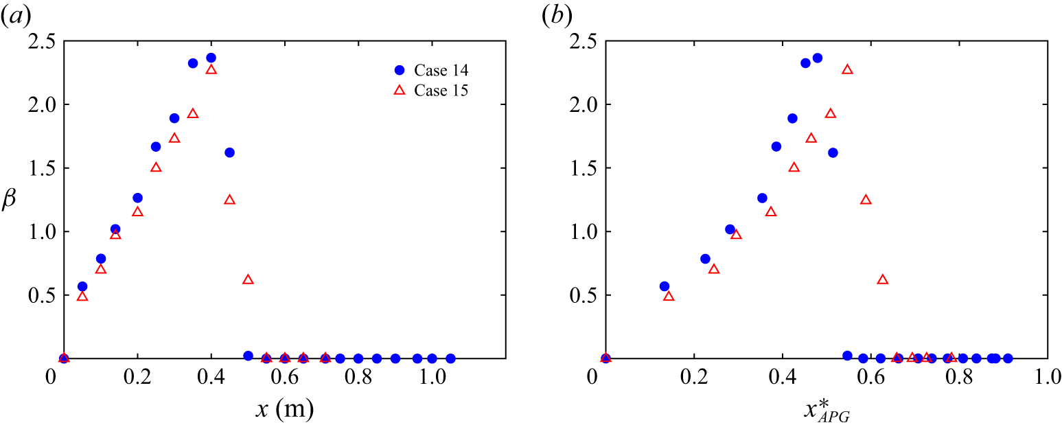
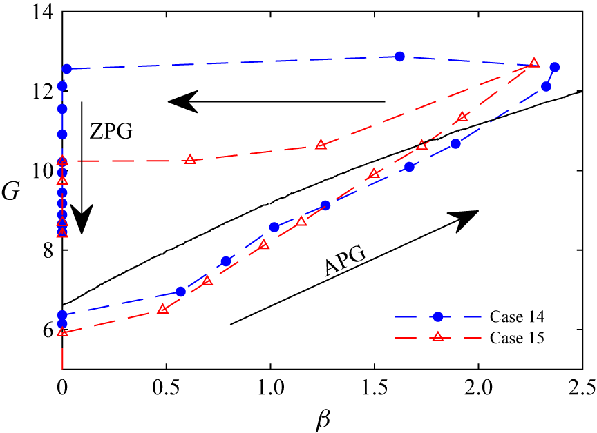
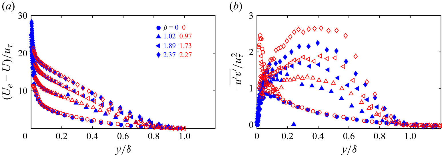
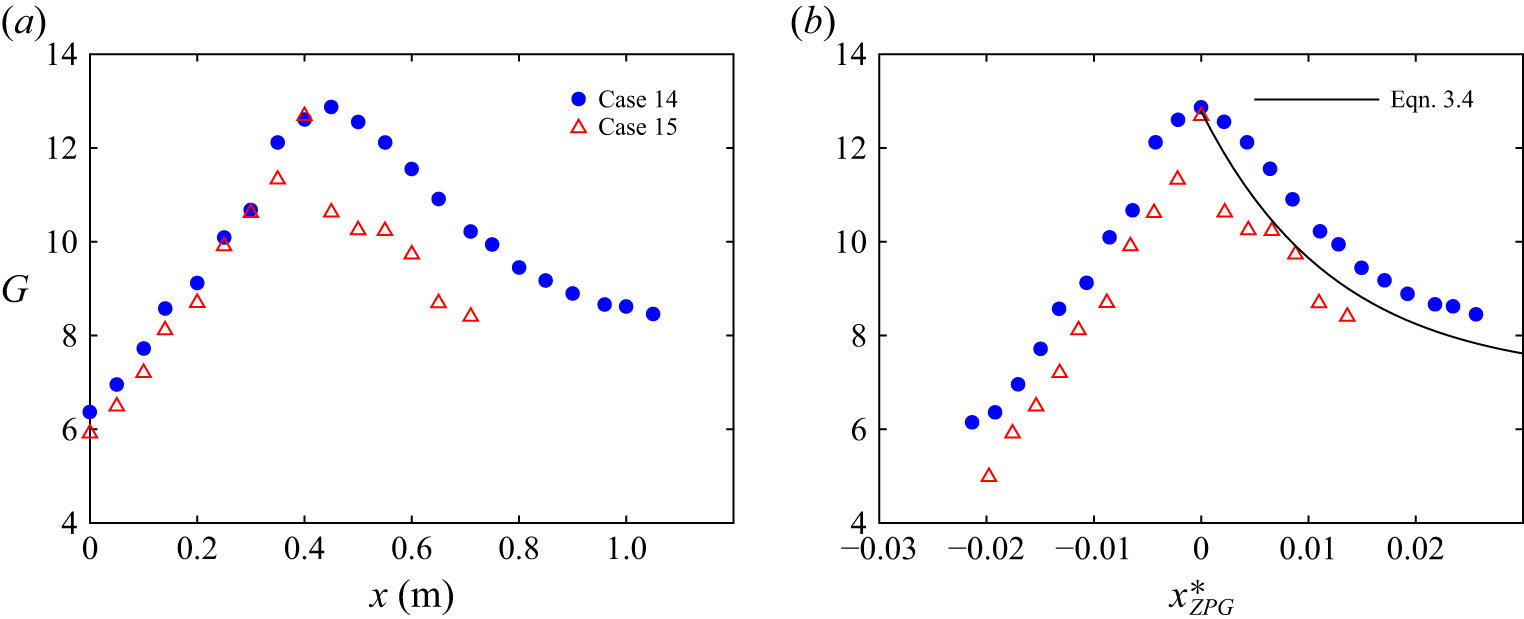
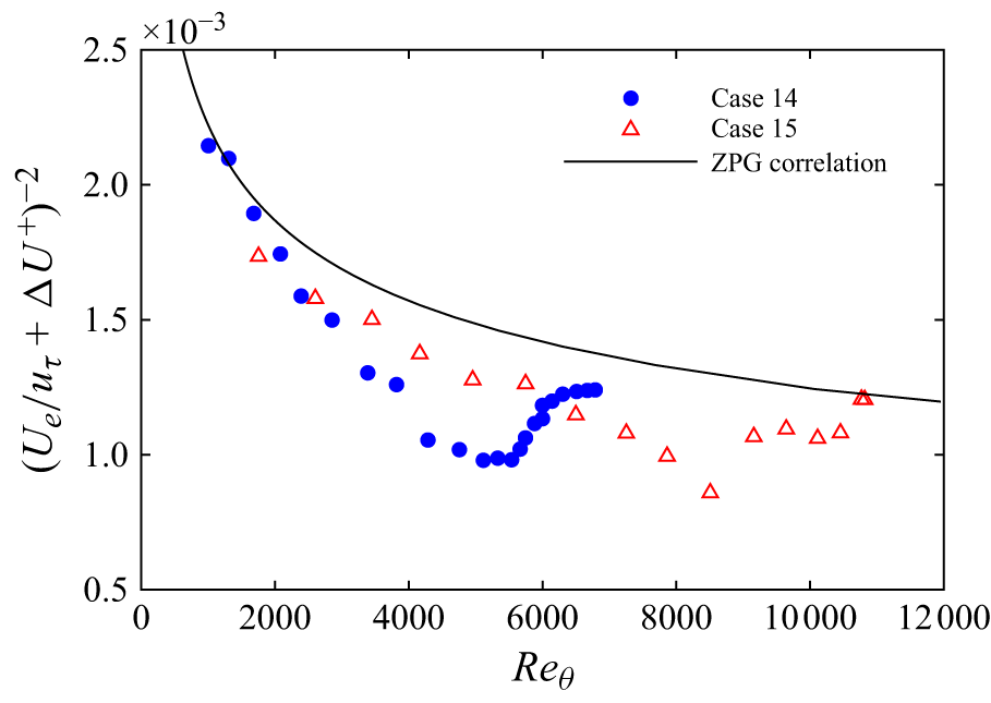
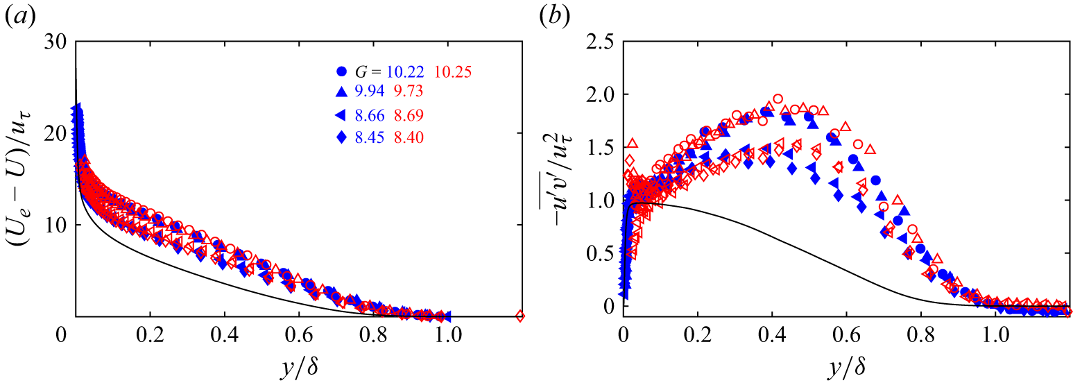
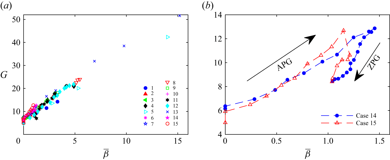
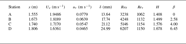
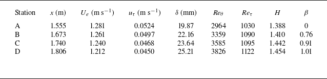
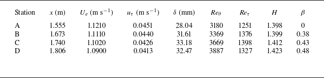
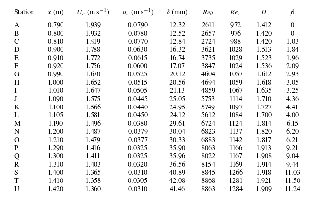
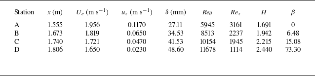
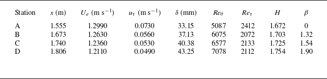
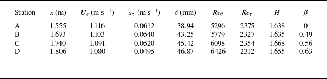
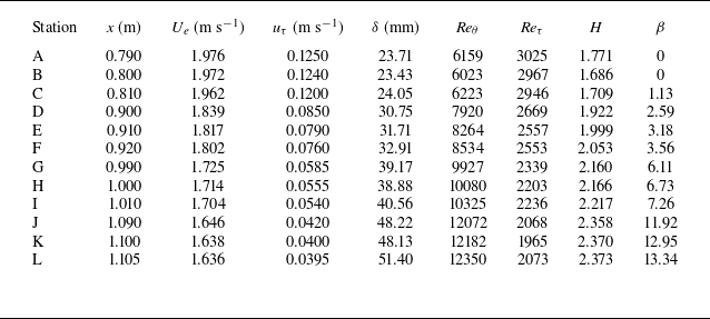
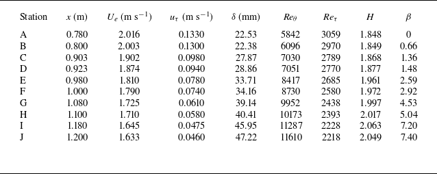
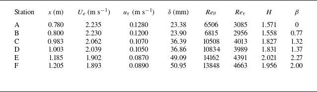
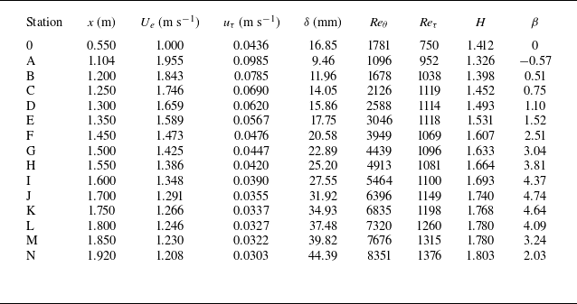
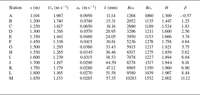
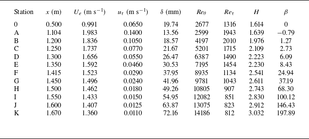
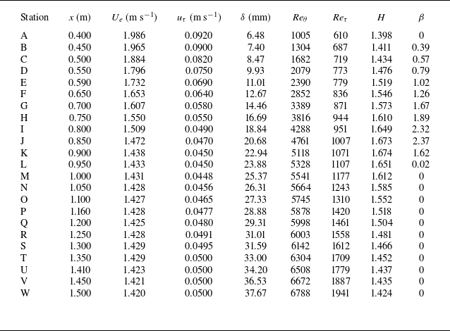
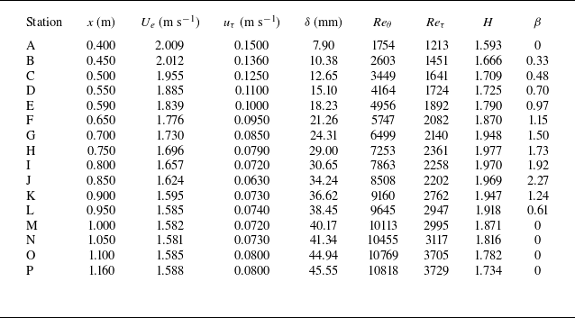

 Open access

