









1 Introduction
The Hilbert transform was introduced by Hilbert in 1912 as part of his investigation of the Riemann problem in the realm of complex analysis [Reference Hilbert38]. Indeed, it may be regarded as the operator describing the boundary behaviour of the harmonic conjugate in the upper half plane. Explicitly, it is given by

Equivalently, it is the Fourier multiplier
$(Hf)^\wedge (\xi ) = i \, \mathrm {sgn}(\xi ) \, \widehat {f}(\xi )$
 [Reference Duoandikoetxea25]. In 1924, M. Riesz proved its
$L_p$
[Reference Duoandikoetxea25]. In 1924, M. Riesz proved its
$L_p$
 -boundedness for all
$p \in 2 \mathbb {Z}_+$
-boundedness for all
$p \in 2 \mathbb {Z}_+$
 using an ad hoc complex analysis argument [Reference Riesz75, Reference Riesz76]. By duality and Marcinkiewicz’s interpolation this yields
$L_p$
using an ad hoc complex analysis argument [Reference Riesz75, Reference Riesz76]. By duality and Marcinkiewicz’s interpolation this yields
$L_p$
 -boundedness for every
$1 < p < \infty $
-boundedness for every
$1 < p < \infty $
 . Afterwards, Kolmogorov and Calderón-Zygmund found proofs giving the weak type
$(1,1)$
. Afterwards, Kolmogorov and Calderón-Zygmund found proofs giving the weak type
$(1,1)$
 [Reference Kolmogorov50, Reference Stein81, Reference Calderón10].
In 1955, Cotlar proved the
$L_p$
 -boundedness of the Hilbert transform through an extremely simple argument [Reference Cotlar17]. He showed that H is
$L_p$
-boundedness of the Hilbert transform through an extremely simple argument [Reference Cotlar17]. He showed that H is
$L_p$
 -bounded for
$p = 2^k$
-bounded for
$p = 2^k$
 recursively – from the trivial case
$p=2$
recursively – from the trivial case
$p=2$
 – using his elegant Cotlar identity

Note that for the Hilbert transform, we have
$H^2=-\text {id} $
 whenever it is well-defined. Therefore, the Cotlar identity above can be rewritten as

A key point in our work is to notice that Cotlar’s identity and its generalizations have a nicer expression at the frequency side of the Fourier transform. As an illustration, notice that a Euclidean Fourier multiplier
$(T_m f)^\wedge (\xi ) = m( \xi ) \, \widehat {f}(\xi )$
 satisfies Cotlar’s identity precisely when

In fact, any bounded function satisfying the classical Cotlar identity above will be bounded on
$L_p(\mathbb {R})$
 for every
$1<p<\infty $
for every
$1<p<\infty $
 . In this article, we will investigate similar identities on more general locally compact groups and their von Neumann algebras. A pioneering work in this direction was due to Mei and Ricard [Reference Mei and Ricard55], where the authors deployed a noncommutative analogue of the Cotlar identity, which holds in the context of amalgamated free product von Neumann algebras. The main goal of this article is to further Mei and Ricard’s technique beyond free groups by illuminating the hidden connection between noncommutative Cotlar identities and group actions on trees and other tree-like structures – like
$\mathbb {R}$
. In this article, we will investigate similar identities on more general locally compact groups and their von Neumann algebras. A pioneering work in this direction was due to Mei and Ricard [Reference Mei and Ricard55], where the authors deployed a noncommutative analogue of the Cotlar identity, which holds in the context of amalgamated free product von Neumann algebras. The main goal of this article is to further Mei and Ricard’s technique beyond free groups by illuminating the hidden connection between noncommutative Cotlar identities and group actions on trees and other tree-like structures – like
$\mathbb {R}$
 -trees and uniquely arcwise connected spaces.
Noncommutative Fourier multipliers. Here we will deal with operators analogous to the Hilbert transform over group algebras. Let
$\mathrm {G}$
 be a locally compact group. Its (left regular) group von Neumann algebra is defined as

When
$\mathrm {G}$
 is Abelian,
$\mathcal {L} \mathrm {G}$
is Abelian,
$\mathcal {L} \mathrm {G}$
 is isomorphic to
$L_\infty (\widehat {\mathrm {G}})$
is isomorphic to
$L_\infty (\widehat {\mathrm {G}})$
 , the
$L_\infty $
, the
$L_\infty $
 -space over the Pontryagin dual of
$\mathrm {G}$
-space over the Pontryagin dual of
$\mathrm {G}$
 . Thus,
$\mathcal {L} \mathrm {G}$
. Thus,
$\mathcal {L} \mathrm {G}$
 behaves as a generalization of the Pontryagin dual for noncommutative groups. When
$\mathrm {G}$
behaves as a generalization of the Pontryagin dual for noncommutative groups. When
$\mathrm {G}$
 is unimodular, the algebra
$\mathcal {L} \mathrm {G}$
is unimodular, the algebra
$\mathcal {L} \mathrm {G}$
 admits a normal, semifinite, and faithful tracial weight called the Plancherel trace [Reference Pedersen67, Chapter 8], with respect to which the noncommutative
$L_p$
admits a normal, semifinite, and faithful tracial weight called the Plancherel trace [Reference Pedersen67, Chapter 8], with respect to which the noncommutative
$L_p$
 -spaces
$L_p(\mathcal {L} \mathrm {G})$
-spaces
$L_p(\mathcal {L} \mathrm {G})$
 are defined [Reference Terp84, Reference Pisier and Xu72]. These
$L_p$
are defined [Reference Terp84, Reference Pisier and Xu72]. These
$L_p$
 -spaces straightforwardly generalize the spaces of
$L_p$
-spaces straightforwardly generalize the spaces of
$L_p$
 -integrable elements over the dual of
$\mathrm {G}$
-integrable elements over the dual of
$\mathrm {G}$
 . As such, many classical problems of Fourier analysis over
$L_p$
. As such, many classical problems of Fourier analysis over
$L_p$
 -spaces find an analogue in the noncommutative setting. A prominent example is the study of the
$L_p$
-spaces find an analogue in the noncommutative setting. A prominent example is the study of the
$L_p$
 -boundedness of Fourier multipliers. Indeed, given
$m: \mathrm {G} \to \mathbb {C}$
-boundedness of Fourier multipliers. Indeed, given
$m: \mathrm {G} \to \mathbb {C}$
 , the Fourier multiplier of symbol m will be the – potentially unbounded – linear operator
$T_m: D \subseteq \mathcal {L} \mathrm {G} \to \mathcal {L} \mathrm {G}$
, the Fourier multiplier of symbol m will be the – potentially unbounded – linear operator
$T_m: D \subseteq \mathcal {L} \mathrm {G} \to \mathcal {L} \mathrm {G}$
 given by linear extension of

The study of bounded Fourier multipliers on
$L_p$
 -spaces of group von Neumann algebras has gained significant attention due to its deep connections with harmonic analysis and group theory. For
$p=\infty $
-spaces of group von Neumann algebras has gained significant attention due to its deep connections with harmonic analysis and group theory. For
$p=\infty $
 , many classical approximation properties of groups can be reformulated in terms of sequences of Fourier multipliers; see [Reference Haagerup36, Reference Cowling and Haagerup18, Reference De Cannière and Haagerup21]. This viewpoint enabled the use of harmonic analysis techniques in group theory and led, for example, to Haagerup’s proof that higher-rank Lie groups are not weakly amenable [Reference Haagerup37]. For
$1< p < \infty $
, many classical approximation properties of groups can be reformulated in terms of sequences of Fourier multipliers; see [Reference Haagerup36, Reference Cowling and Haagerup18, Reference De Cannière and Haagerup21]. This viewpoint enabled the use of harmonic analysis techniques in group theory and led, for example, to Haagerup’s proof that higher-rank Lie groups are not weakly amenable [Reference Haagerup37]. For
$1< p < \infty $
 , the analogous approximation property on
$L_p$
, the analogous approximation property on
$L_p$
 was studied by Lafforgue, de la Salle and de Laat [Reference Lafforgue and de la Salle51, Reference de Laat and De la Salle23], who showed that lattices in higher-rank Lie groups do not admit uniformly bounded Fourier multiplier approximate units on
$L_p$
was studied by Lafforgue, de la Salle and de Laat [Reference Lafforgue and de la Salle51, Reference de Laat and De la Salle23], who showed that lattices in higher-rank Lie groups do not admit uniformly bounded Fourier multiplier approximate units on
$L_p$
 , for a range of p that increases with the rank. Determining the exact range of exponents and whether the critical threshold
$p_0$
, for a range of p that increases with the rank. Determining the exact range of exponents and whether the critical threshold
$p_0$
 encodes the rank remains a major open question [Reference Parcet, Ricard and de la Salle65, Reference Conde-Alonso, González-Pérez, Parcet and Tablate15, Reference de la Salle22, Reference Parcet63].
Fourier multipliers are also interesting for purely analytical reasons. Many long-standing problems in harmonic analysis on
$\mathbb {R}^n$
 can be formulated in terms of
$L_p$
can be formulated in terms of
$L_p$
 -bounded multipliers; see, for example, [Reference Tao82] and [Reference Tao83, Lecture 5]. Consequently, a complete characterization of bounded Fourier multipliers is not expected beyond the cases
$p = 1, 2$
-bounded multipliers; see, for example, [Reference Tao82] and [Reference Tao83, Lecture 5]. Consequently, a complete characterization of bounded Fourier multipliers is not expected beyond the cases
$p = 1, 2$
 ,
$\infty $
,
$\infty $
 . Finding sufficient conditions for the boundedness of Fourier multipliers in the group setting presents additional challenges that do not arise in the abelian case. First, the definition of the
$L_p$
. Finding sufficient conditions for the boundedness of Fourier multipliers in the group setting presents additional challenges that do not arise in the abelian case. First, the definition of the
$L_p$
 -spaces requires working within von Neumann algebras, where many of the necessary functional-analytic tools, such as operator space theory [Reference Effros and Ruan26, Reference Pisier70, Reference Pisier71], mixed-norm
$L_p$
-spaces requires working within von Neumann algebras, where many of the necessary functional-analytic tools, such as operator space theory [Reference Effros and Ruan26, Reference Pisier70, Reference Pisier71], mixed-norm
$L_p$
 -spaces [Reference Pisier69, Reference Junge42, Reference Junge and Parcet46], and maximal inequalities [Reference Cuculescu19, Reference Lance52, Reference Junge and Xu48, Reference Cadilhac and Ricard9], were fully developed only in the past two decades. A second major difficulty is the lack, in the von Neumann algebra setting, of many singular integral techniques that are fundamental in the analysis on
$\mathbb {R}^n$
-spaces [Reference Pisier69, Reference Junge42, Reference Junge and Parcet46], and maximal inequalities [Reference Cuculescu19, Reference Lance52, Reference Junge and Xu48, Reference Cadilhac and Ricard9], were fully developed only in the past two decades. A second major difficulty is the lack, in the von Neumann algebra setting, of many singular integral techniques that are fundamental in the analysis on
$\mathbb {R}^n$
 . Although there has been progress toward a noncommutative Calderón-Zygmund theory [Reference Parcet62, Reference González-Pérez, Junge and Parcet33, Reference Junge, Mei, Parcet and Xia45, Reference Cadilhac, Conde-Alonso and Parcet8], a comprehensive theory capable of producing weak type
$(1,1)$
. Although there has been progress toward a noncommutative Calderón-Zygmund theory [Reference Parcet62, Reference González-Pérez, Junge and Parcet33, Reference Junge, Mei, Parcet and Xia45, Reference Cadilhac, Conde-Alonso and Parcet8], a comprehensive theory capable of producing weak type
$(1,1)$
 bounds remains unavailable outside semicommutative or nilpotent contexts. These technical obstacles have significantly delayed the systematic study of Fourier multipliers on noncommutative
$L_p$
bounds remains unavailable outside semicommutative or nilpotent contexts. These technical obstacles have significantly delayed the systematic study of Fourier multipliers on noncommutative
$L_p$
 -spaces until relatively recently.
As hinted before, one possible way of overcoming the lack of a Calderón-Zygmund theory was found in Mei and Ricard’s article [Reference Mei and Ricard55]. Their noncommutative analogue of the Cotlar identity allowed them to prove that functions
$m: \mathbb {F}_2 \to \mathbb {C}$
 over the free group whose value
$m(\omega )$
over the free group whose value
$m(\omega )$
 depends only on the starting letter
$\{a, a^{-1}, b, b^{-1}\}$
depends only on the starting letter
$\{a, a^{-1}, b, b^{-1}\}$
 of the reduced word
$\omega \in \mathbb {F}_2$
of the reduced word
$\omega \in \mathbb {F}_2$
 give rise to bounded Fourier multipliers on
$L_p$
give rise to bounded Fourier multipliers on
$L_p$
 , i.e.,

In this article, we will study a new geometric way to define
$L_p$
 -bounded Fourier multipliers on groups admitting actions on tree-like structures, and we will see in Section 5 that this recovers (MR) as a particular example.
Noncommutative Cotlar identities. Let
$\mathrm {G}_0 \subseteq \mathrm {G}$
 be an open subgroup of the locally compact and unimodular group
$\mathrm {G}$
be an open subgroup of the locally compact and unimodular group
$\mathrm {G}$
 . It is trivial to see that
$\mathrm {G}_0$
. It is trivial to see that
$\mathrm {G}_0$
 is also unimodular and that
$\mathcal {L} \mathrm {G}_0 \subseteq \mathcal {L} \mathrm {G}$
is also unimodular and that
$\mathcal {L} \mathrm {G}_0 \subseteq \mathcal {L} \mathrm {G}$
 is a complemented inclusion, that is, an inclusion admitting a normal conditional expectation
$\mathbb {E}: \mathcal {L} \mathrm {G} \to \mathcal {L} \mathrm {G}_0$
is a complemented inclusion, that is, an inclusion admitting a normal conditional expectation
$\mathbb {E}: \mathcal {L} \mathrm {G} \to \mathcal {L} \mathrm {G}_0$
 . We will say that a (potentially unbounded) multiplier
$T_m$
. We will say that a (potentially unbounded) multiplier
$T_m$
 satisfies a noncommutative Cotlar identity with respect to the von Neumann subalgebra
$\mathcal {L} \mathrm {G}_0$
satisfies a noncommutative Cotlar identity with respect to the von Neumann subalgebra
$\mathcal {L} \mathrm {G}_0$
 iff
iff

where
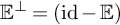
$\mathbb {E}^\perp = (\mathrm {id} - \mathbb {E})$
 .
.
We have distilled an easily verifiable closed formula (Cotla ^r) for m that is equivalent to (Cotlar) above; see Theorem 2.4. Since with an additional assumption on the symbol, the Cotlar formula implies
$L_p$
 -boundedness, we obtain the following theorem.
Theorem A. Let
$\mathrm {G}$
 be a locally compact unimodular group,
$\mathrm {G}_0 \subseteq \mathrm {G}$
be a locally compact unimodular group,
$\mathrm {G}_0 \subseteq \mathrm {G}$
 a closed subgroup and
$m: \mathrm {G} \to \mathbb {C}$
a closed subgroup and
$m: \mathrm {G} \to \mathbb {C}$
 a left
$\mathrm {G}_0$
a left
$\mathrm {G}_0$
 -invariant bounded and measurable function. If m satisfies that

then
$T_m$
 is
$L_p$
is
$L_p$
 -bounded for
$1<p<\infty $
-bounded for
$1<p<\infty $
 and furthermore

The theorem above decouples into two different statements depending on whether
$\mathrm {G}_0 \subseteq \mathrm {G}$
 is open or has empty interior. In the case of an open subgroup, it holds that
$0 < \mu (\mathrm {G}_0)$
is open or has empty interior. In the case of an open subgroup, it holds that
$0 < \mu (\mathrm {G}_0)$
 and thus condition (Cotla ^r) has to be verified in a non-total set of pairs
$g, \, h$
and thus condition (Cotla ^r) has to be verified in a non-total set of pairs
$g, \, h$
 . In this case, the associated Fourier multiplier
$T_m$
. In this case, the associated Fourier multiplier
$T_m$
 satisfies (Cotlar) relative to the conditional expectation from
$\mathcal {L} \mathrm {G}$
satisfies (Cotlar) relative to the conditional expectation from
$\mathcal {L} \mathrm {G}$
 to
$\mathcal {L} \mathrm {G}_0$
to
$\mathcal {L} \mathrm {G}_0$
 . In contrast, in the case of a subgroup
$\mathrm {G}_0$
. In contrast, in the case of a subgroup
$\mathrm {G}_0$
 of empty interior we have that
$\mu (\mathrm {G}_0) = 0$
of empty interior we have that
$\mu (\mathrm {G}_0) = 0$
 and thus (Cotla ^r) has to be verified almost everywhere, in which case its associated Fourier multiplier satisfies the non-relative version of the Cotlar identity (Cotlarnr); see below. Furthermore, in the case of
$\mathrm {G}_0$
and thus (Cotla ^r) has to be verified almost everywhere, in which case its associated Fourier multiplier satisfies the non-relative version of the Cotlar identity (Cotlarnr); see below. Furthermore, in the case of
$\mathrm {G}_0$
 of empty interior, the condition of
$m: \mathrm {G} \to \mathbb {C}$
of empty interior, the condition of
$m: \mathrm {G} \to \mathbb {C}$
 being left
$\mathrm {G}_0$
being left
$\mathrm {G}_0$
 -invariant can be dropped, see Remark 2.5. Although our most novel examples would be discrete groups, the case of
$\mu (\mathrm {G}_0) = 0$
-invariant can be dropped, see Remark 2.5. Although our most novel examples would be discrete groups, the case of
$\mu (\mathrm {G}_0) = 0$
 is still useful as it recovers the classical case of the Hilbert transform on
$\mathbb {R}$
is still useful as it recovers the classical case of the Hilbert transform on
$\mathbb {R}$
 .
.
The first advantage of the result above is that it makes the verification of the Cotlar identity for previously known cases almost trivial. Indeed, restricting ourselves to the discrete case for clarity, we can easily show that it holds in the following situations.
-
(1) Classical case. In the classical case of $\mathrm {G} = \mathbb {Z}$
 and
$\mathrm {G}_0 =\{0\}$
with
$m(x) = \mathrm {sgn}(x)$
we only have to verify that either
$m(x+y) = m(x)$
or
$m(-x) = m(y)$
. But that is trivial since either x and y have different signs or
$x + y$
and x share the same sign.
and
$\mathrm {G}_0 =\{0\}$
with
$m(x) = \mathrm {sgn}(x)$
we only have to verify that either
$m(x+y) = m(x)$
or
$m(-x) = m(y)$
. But that is trivial since either x and y have different signs or
$x + y$
and x share the same sign. -
(2) Free product case. If $\mathrm {G} = \mathrm {G}_1 \ast \mathrm {G}_1$
and
$\mathrm {G}_0 = \{e\}$
with both
$\mathrm {G}_2$
and
$\mathrm {G}_2$
discrete, then any function
$m(\omega )$
such that its value depends on the first letter of the reduced word of g satisfies (Cotla ^r). Indeed, we need to prove that either
$m(g h) = m(g)$
or that
$m(g^{-1}) = m(h)$
. Assume the first equality fails, then the first letter of
$g h$
and that of g are different, but that can only happen if the reduced word of h begins with the reduced word of
$g^{-1}$
. If that is the case
$g^{-1}$
and h have the same starting letter and thus
$m(g^{-1}) = m(h)$
. This family of examples was explored by Mei and Ricard [Reference Mei and Ricard55].














A natural question that we answer affirmatively is whether there are examples of groups that go beyond those two categories. In order to explore that question it seems natural to search for bounded functions
$m: \mathrm {G}\to \mathbb {C}$
 satisfying (Cotla ^r) with
$\mathrm {G}$
satisfying (Cotla ^r) with
$\mathrm {G}$
 having Serre’s property
$(\mathrm {FA})$
having Serre’s property
$(\mathrm {FA})$
 [Reference Serre79]. A group
$\mathrm {G}$
[Reference Serre79]. A group
$\mathrm {G}$
 is said to have Serre’s property (FA) iff every orientation-preserving action of
$\mathrm {G}$
is said to have Serre’s property (FA) iff every orientation-preserving action of
$\mathrm {G}$
 on a tree has a global fixed point (a vertex in the tree which is fixed by the action of any
$g\in \mathrm {G}$
on a tree has a global fixed point (a vertex in the tree which is fixed by the action of any
$g\in \mathrm {G}$
 ). More deeply, Serre proved that a discrete group
$\mathrm {G}$
). More deeply, Serre proved that a discrete group
$\mathrm {G}$
 has property
$(\mathrm {FA})$
has property
$(\mathrm {FA})$
 iff it is finitely generated, it does not possess a quotient isomorphic to
$\mathbb {Z}$
iff it is finitely generated, it does not possess a quotient isomorphic to
$\mathbb {Z}$
 and it cannot be expressed as a nontrivial amalgamated free product
$\mathrm {G} = \mathrm {G}_1 \ast _{A} \mathrm {G}_2$
and it cannot be expressed as a nontrivial amalgamated free product
$\mathrm {G} = \mathrm {G}_1 \ast _{A} \mathrm {G}_2$
 . Therefore a group with property
$(\mathrm {FA})$
. Therefore a group with property
$(\mathrm {FA})$
 is excluded from cases 1 and 2. Although there are interesting examples with property
$(\mathrm {FA})$
is excluded from cases 1 and 2. Although there are interesting examples with property
$(\mathrm {FA})$
 , we also give applications to groups like Baumslag-Solitar groups
$\mathrm {BS}(1,m)$
, we also give applications to groups like Baumslag-Solitar groups
$\mathrm {BS}(1,m)$
 and the Bianchi group
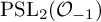
$\mathrm {PSL}_2(\mathcal {O}_{-1})$
and the Bianchi group
$\mathrm {PSL}_2(\mathcal {O}_{-1})$
 , which, despite failing property
$(\mathrm {FA})$
, which, despite failing property
$(\mathrm {FA})$
 , admit bounded functions satisfying Cotlar’s identity for reasons unrelated to them having
$\mathbb {Z}$
, admit bounded functions satisfying Cotlar’s identity for reasons unrelated to them having
$\mathbb {Z}$
 -quotients or being free products.
Groups acting on uniquely arcwise connected spaces. The closed formula in (Cotla ^r) highlights a surprising connection between Cotlar’s identity and geometric group theory. A topological space X is arcwise connected iff given two points
$x, y \in X$
 there exists an injective continuous path
$\gamma : [0,1] \to X$
there exists an injective continuous path
$\gamma : [0,1] \to X$
 joining x and y. An arcwise connected space will be said to be a uniquely arcwise connected space or UAC space iff the path joining x and y is unique [Reference Bestvina, Daverman and Sher5]. Let
$\mathrm {G} \curvearrowright X$
joining x and y. An arcwise connected space will be said to be a uniquely arcwise connected space or UAC space iff the path joining x and y is unique [Reference Bestvina, Daverman and Sher5]. Let
$\mathrm {G} \curvearrowright X$
 be a topological action on a UAC space and fix a root
$x_0 \in X$
be a topological action on a UAC space and fix a root
$x_0 \in X$
 with
$\mathrm {G}_0$
with
$\mathrm {G}_0$
 being the stabilizer
$\mathrm {St}_{x_0}$
being the stabilizer
$\mathrm {St}_{x_0}$
 of
$x_0$
of
$x_0$
 . Observe that
$X \setminus \{x_0\}$
. Observe that
$X \setminus \{x_0\}$
 is given by

where each
$X_\beta $
 is arcwise connected. The decomposition into disjoint sets in identity (1.2) above is, a priori, purely set-theoretic, and we do not assume the sets
$X_\beta $
is arcwise connected. The decomposition into disjoint sets in identity (1.2) above is, a priori, purely set-theoretic, and we do not assume the sets
$X_\beta $
 to be closed. Observe that the action of
$\mathrm {G}_0$
to be closed. Observe that the action of
$\mathrm {G}_0$
 restricted to
$X \setminus \{x_0\}$
restricted to
$X \setminus \{x_0\}$
 permutes the sets
$X_\beta $
permutes the sets
$X_\beta $
 . The following theorem gives a machinery to get multipliers satisfying Cotlar’s identity from actions on UAC spaces.
Theorem B. Let
$\mathrm {G} \curvearrowright X$
 be a topological action on a UAC space. Fix
$x_0 \in X$
be a topological action on a UAC space. Fix
$x_0 \in X$
 ,
$\mathrm {G}_0$
,
$\mathrm {G}_0$
 being the stabilizer of
$x_0$
being the stabilizer of
$x_0$
 , i.e.,
$\mathrm {G}_0= \mathrm {St}_{x_0}$
, i.e.,
$\mathrm {G}_0= \mathrm {St}_{x_0}$
 , and let
$\widetilde {m}: X \to \mathbb {C}$
, and let
$\widetilde {m}: X \to \mathbb {C}$
 be a bounded function satisfying that
-
(i) $\widetilde {m}$
is constant over each
$X_\beta $
of (1.2). -
(ii) $\widetilde {m}$
is constant over
$\mathrm {G}_0$
orbits, i.e.,
$\, \widetilde {m}{|}_{X_\beta } = \widetilde {m}{|}_{X_\alpha }$
if there is an element
$h \in \mathrm {G}_0$
such that
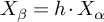
$X_\beta = h \cdot X_\alpha $
.




Then the function
$m: \mathrm {G} \to \mathbb {C}$
 given by
$m(g) \, = \, \widetilde {m}(g \cdot x_0)$
given by
$m(g) \, = \, \widetilde {m}(g \cdot x_0)$
 satisfies (Cotla ^r) and therefore Theorem A applies.
The proof of Theorem B is so neat that it can be tightly summarized here.
First, notice that condition (ii) ensures that m is left-
$\mathrm {G}_0$
 -invariant. Condition (i), on the other hand, implies that (Cotla ^r) holds. To see this, assume that
$m(gh) \neq m(g)$
-invariant. Condition (i), on the other hand, implies that (Cotla ^r) holds. To see this, assume that
$m(gh) \neq m(g)$
 . Since the two values are different, the arcwise connected subsets of
$X \setminus \{x_0\}$
. Since the two values are different, the arcwise connected subsets of
$X \setminus \{x_0\}$
 containing
$g h \cdot x_0$
containing
$g h \cdot x_0$
 and
$g \cdot x_0$
and
$g \cdot x_0$
 must be different, see Figure 1. Thus, there is a unique arc joining these two points that passes through
$x_0$
must be different, see Figure 1. Thus, there is a unique arc joining these two points that passes through
$x_0$
 . Applying
$g^{-1}$
. Applying
$g^{-1}$
 to this arc, since
$\mathcal {G}$
to this arc, since
$\mathcal {G}$
 acts by homeomorphisms, we get an arc starting at
$x_0$
acts by homeomorphisms, we get an arc starting at
$x_0$
 that passes through
$g^{-1} \cdot x_0$
that passes through
$g^{-1} \cdot x_0$
 and then
$h \cdot x_0$
and then
$h \cdot x_0$
 . It follows that
$g^{-1} \cdot x_0$
. It follows that
$g^{-1} \cdot x_0$
 and
$h \cdot x_0$
and
$h \cdot x_0$
 lie in the same arcwise connected subset of
$X \setminus \{x_0\}$
lie in the same arcwise connected subset of
$X \setminus \{x_0\}$
 and thus
$m(h) = m(g^{-1})$
and thus
$m(h) = m(g^{-1})$
 . By Remarks 2.5 and 3.2, condition (ii) can be dropped when the interior of
$\mathrm {St}_{x_0}$
. By Remarks 2.5 and 3.2, condition (ii) can be dropped when the interior of
$\mathrm {St}_{x_0}$
 is empty.
Action over paths.

Left-orderable groups. A family of examples that fits right into the model of Theorem A is that of left-orderable groups. Those are groups admitting a total or linear order
$(\mathrm {G}, \preceq )$
 that is invariant under left translations, i.e.,
$g \preceq h\, \Longleftrightarrow \, a g \preceq a h$
that is invariant under left translations, i.e.,
$g \preceq h\, \Longleftrightarrow \, a g \preceq a h$
 for every
$a, g, h \in \mathrm {G}$
for every
$a, g, h \in \mathrm {G}$
 . We will write
$g \prec h$
. We will write
$g \prec h$
 when
$g \preceq h$
when
$g \preceq h$
 but
$g \neq h$
but
$g \neq h$
 . For left-orderable groups the following result holds for their sign function.
Theorem C. Let
$\mathrm {G}$
 be a left-orderable group and
$\mathrm {sgn}: \mathrm {G} \to \mathbb {C}$
be a left-orderable group and
$\mathrm {sgn}: \mathrm {G} \to \mathbb {C}$
 be the function

Then
$H = T_{\mathrm {sgn}}: L_p(\mathcal {L} \mathrm {G}) \to L_p(\mathcal {L} \mathrm {G})$
 satisfies that

The boundedness of H in Theorem C can be obtained by showing directly that (Cotla ^r) holds. Alternatively, it is known that a countable group is left-orderable iff it acts faithfully on
$\mathbb {R}$
 by order-preserving homeomorphisms, see for instance [Reference Navas60, Proposition 2.1]. The observation that
$\mathbb {R}$
by order-preserving homeomorphisms, see for instance [Reference Navas60, Proposition 2.1]. The observation that
$\mathbb {R}$
 is a UAC space allows us to prove the result as a consequence of Theorem B. In principle, proving Cotlar’s identity gives just that the
$L_p$
is a UAC space allows us to prove the result as a consequence of Theorem B. In principle, proving Cotlar’s identity gives just that the
$L_p$
 -norm grows like
$\mathrm {O}(p^\beta )$
-norm grows like
$\mathrm {O}(p^\beta )$
 with
$\beta = \log _2(1 + \sqrt {2})$
with
$\beta = \log _2(1 + \sqrt {2})$
 , as
$p \to \infty $
, as
$p \to \infty $
 . Nevertheless, a more careful argument allows us to show that the constant can be lowered down to the optimal order
$\mathrm {O}(p)$
. Nevertheless, a more careful argument allows us to show that the constant can be lowered down to the optimal order
$\mathrm {O}(p)$
 , as long as
$m(g) \overline {m(g^{-1})} = -1$
, as long as
$m(g) \overline {m(g^{-1})} = -1$
 for
$g \in \mathrm {G} \setminus \{e\}$
for
$g \in \mathrm {G} \setminus \{e\}$
 , see Corollary 2.8. It is also worth noticing that the above transforms for left-orderable group algebras can be seen as a particular example of the Hilbert transforms associated with Arveson’s subdiagonal algebras [Reference Arveson2], for which the weak type
$(1,1)$
, see Corollary 2.8. It is also worth noticing that the above transforms for left-orderable group algebras can be seen as a particular example of the Hilbert transforms associated with Arveson’s subdiagonal algebras [Reference Arveson2], for which the weak type
$(1,1)$
 was proved by Randrianantoanina [Reference Randrianantoanina74], see also [Reference Pisier and Xu72, Theorem 8.4]. Therefore our geometric model in Theorem B generalizes simultaneously Mei and Ricard’s free Hilbert transforms and subdiagonal Hilbert transforms, recovering the best known constants in both cases. Left-orderable groups include:
-
• Torsion-free Abelian groups;
-
• Torsion-free nilpotent groups;
-
• Free groups $\mathbb {F}_r$
; -
• Braid groups $B_n$
; -
• Right-angled Artin groups;
-
• Baumslag-Solitar groups $\mathrm {BS}(1, n)$
for
$n \geq 2$
; -
• Surface groups;
-
• The Thompson group F.


It is possible to obtain explicit examples of
$L_p$
 -bounded Fourier multipliers satisfying Cotlar’s identity in each of these families of groups. Furthermore, there are known examples of left-orderable groups that have Serre’s property
$(\mathrm {FA})$
-bounded Fourier multipliers satisfying Cotlar’s identity in each of these families of groups. Furthermore, there are known examples of left-orderable groups that have Serre’s property
$(\mathrm {FA})$
 . Some of these examples arise from groups of isometries of the hyperbolic plane. For instance, let
$D(2,3,7)$
. Some of these examples arise from groups of isometries of the hyperbolic plane. For instance, let
$D(2,3,7)$
 denote the
$(2,3,7)$
denote the
$(2,3,7)$
 von Dyck group (sometimes called the ‘ordinary’ triangle group). This is the group of orientation-preserving isometries of a tiling of the hyperbolic plane by geodesic triangles with angles
$\frac {\pi }{2}$
von Dyck group (sometimes called the ‘ordinary’ triangle group). This is the group of orientation-preserving isometries of a tiling of the hyperbolic plane by geodesic triangles with angles
$\frac {\pi }{2}$
 ,
$\frac {\pi }{3}$
,
$\frac {\pi }{3}$
 and
$\frac {\pi }{7}$
and
$\frac {\pi }{7}$
 .
$D(2,3,7)$
.
$D(2,3,7)$
 admits a presentation as follows.

Let
$\widetilde {\mathrm {PSL}}_2(\mathbb {R}) \twoheadrightarrow \mathrm {PSL}_2(\mathbb {R})$
 be the universal cover of
$\mathrm {PSL}_2(\mathbb {R})$
be the universal cover of
$\mathrm {PSL}_2(\mathbb {R})$
 . The lifting
$\Gamma $
. The lifting
$\Gamma $
 of
$D(2,3,7)$
of
$D(2,3,7)$
 to
$\widetilde {\mathrm {PSL}}_2(\mathbb {R})$
to
$\widetilde {\mathrm {PSL}}_2(\mathbb {R})$
 is an example of a group with Serre’s property
$(\mathrm {FA})$
is an example of a group with Serre’s property
$(\mathrm {FA})$
 that is also left-orderable [Reference Bergman4, Reference Cornulier and Kar16, Reference Khoi49, Reference Serre79]. See the proof of Proposition 5.5.
Graphs of groups and Bass-Serre theory. A wealth of examples of multipliers satisfying (Cotla ^r) can be obtained from Bass-Serre theory – which allows us to classify groups acting on trees without edge inversions – see [Reference Serre79]. Indeed, given a group acting on a tree
$\mathrm {G} \curvearrowright T$
 , it is possible to build a graph by taking the quotient with respect to the action
$X = T/\mathrm {G}$
, it is possible to build a graph by taking the quotient with respect to the action
$X = T/\mathrm {G}$
 and associating to each vertex and to each edge its corresponding stabilizer. Due to the lack of edge inversions, the stabilizer of an edge embeds into the stabilizers of its extremes. This structure – a graph with groups on its edges and vertices and such that the groups at the edges embed into the extremes of said edge – is called a graph of groups. Let us denote it by
$\mathbb {X}$
and associating to each vertex and to each edge its corresponding stabilizer. Due to the lack of edge inversions, the stabilizer of an edge embeds into the stabilizers of its extremes. This structure – a graph with groups on its edges and vertices and such that the groups at the edges embed into the extremes of said edge – is called a graph of groups. Let us denote it by
$\mathbb {X}$
 . Like in the case of graphs, it is possible to define a sort of universal cover of
$\mathbb {X}$
. Like in the case of graphs, it is possible to define a sort of universal cover of
$\mathbb {X}$
 such that its underlying graph is a tree
$\widetilde {X}$
such that its underlying graph is a tree
$\widetilde {X}$
 and its fundamental group
$\pi _1(\mathbb {X})$
and its fundamental group
$\pi _1(\mathbb {X})$
 acts as deck transformations of the covering. The main point of the theory is that
$\pi _1(\mathbb {X}) \cong \mathrm {G}$
acts as deck transformations of the covering. The main point of the theory is that
$\pi _1(\mathbb {X}) \cong \mathrm {G}$
 and the action of
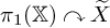
$\pi _1(\mathbb {X}) \curvearrowright \widetilde {X}$
and the action of
$\pi _1(\mathbb {X}) \curvearrowright \widetilde {X}$
 recovers
$\mathrm {G} \curvearrowright T$
recovers
$\mathrm {G} \curvearrowright T$
 .
.
Our main theorem in Section 5 would be that the multiplier results for symbols depending on the starting letter, like inequality (MR) from [Reference Mei and Ricard55], extend from free products to general graphs of groups. Let us fix some notation. First, when working with a graph of groups, we will consider that our graph is oriented, that both directions of the edge occur and that there can be both loops and multiple edges between two given vertices. As it is customary, given an edge y, we will denote by
$\bar {y}$
 the reverse edge and by
$\mathrm {o}(y) \in \mathrm {Vert}(X)$
the reverse edge and by
$\mathrm {o}(y) \in \mathrm {Vert}(X)$
 and
$\mathrm {t}(y) \in \mathrm {Vert}(X)$
and
$\mathrm {t}(y) \in \mathrm {Vert}(X)$
 the origin and target vertices of the edge. An orientation would be a subset
$\mathrm {Edge}_+ \subseteq \mathrm {Edge}$
the origin and target vertices of the edge. An orientation would be a subset
$\mathrm {Edge}_+ \subseteq \mathrm {Edge}$
 that contains either y or
$\bar {y}$
that contains either y or
$\bar {y}$
 for each edge. We will also denote by
$\mathrm {G}_x$
for each edge. We will also denote by
$\mathrm {G}_x$
 the groups associated to vertices and by
$\mathrm {H}_y$
the groups associated to vertices and by
$\mathrm {H}_y$
 the groups associated to edges. By construction, we have that
$\mathrm {H}_y = \mathrm {H}_{\bar {y}}$
the groups associated to edges. By construction, we have that
$\mathrm {H}_y = \mathrm {H}_{\bar {y}}$
 and that there are injective homomorphisms
$\alpha _y: \mathrm {H}_y \to \mathrm {G}_{\mathrm {t}(y)}$
and that there are injective homomorphisms
$\alpha _y: \mathrm {H}_y \to \mathrm {G}_{\mathrm {t}(y)}$
 and
$\alpha _{\bar {y}}: \mathrm {H}_y \to \mathrm {G}_{\mathrm {o}(y)}$
and
$\alpha _{\bar {y}}: \mathrm {H}_y \to \mathrm {G}_{\mathrm {o}(y)}$
 . We will denote the image group
$\alpha _y[\mathrm {H}_y] \subseteq \mathrm {G}_{\mathrm {t}(y)}$
. We will denote the image group
$\alpha _y[\mathrm {H}_y] \subseteq \mathrm {G}_{\mathrm {t}(y)}$
 by
$\mathrm {H}_y^y$
by
$\mathrm {H}_y^y$
 . Similarly
$\mathrm {H}_{\bar {y}}^{\bar {y}}$
. Similarly
$\mathrm {H}_{\bar {y}}^{\bar {y}}$
 will denote the image of
$\alpha _{\bar {y}}$
will denote the image of
$\alpha _{\bar {y}}$
 . We can now recall the construction of
$\pi _1(\mathbb {X})$
. We can now recall the construction of
$\pi _1(\mathbb {X})$
 . Define the auxiliary group
$F(\mathbb {X})$
. Define the auxiliary group
$F(\mathbb {X})$
 as the free product of all the groups
$\mathrm {G}_x$
as the free product of all the groups
$\mathrm {G}_x$
 – where x runs over the vertex set
$\mathrm {Vert}(X)$
– where x runs over the vertex set
$\mathrm {Vert}(X)$
 – together with
$\mathbb {F}_{\mathrm {Edge}(X)}$
– together with
$\mathbb {F}_{\mathrm {Edge}(X)}$
 , the free group generated by all the edges, with the following extra relations imposed

To construct the fundamental group, assume X is connected and choose a base point
$x_0 \in \mathrm {Vert}(X)$
 . A closed path c that starts and ends at
$x_0$
. A closed path c that starts and ends at
$x_0$
 will be a sequence of edges
$c = y_1 \, y_2 \, \cdots y_m$
will be a sequence of edges
$c = y_1 \, y_2 \, \cdots y_m$
 , with
$\mathrm {t}(y_i) = \mathrm {o}(y_{i+1})$
, with
$\mathrm {t}(y_i) = \mathrm {o}(y_{i+1})$
 and
$\mathrm {o}(y_1) = x_0 = \mathrm {t}(y_m)$
and
$\mathrm {o}(y_1) = x_0 = \mathrm {t}(y_m)$
 . The group
$\pi _1(\mathbb {X},x_0)$
. The group
$\pi _1(\mathbb {X},x_0)$
 is given by the subset of
$F(\mathbb {X})$
is given by the subset of
$F(\mathbb {X})$
 of elements of the form:

where
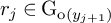
$r_j \in \mathrm {G}_{\mathrm {o}(y_{j+1})}$
 for
$j \leq m -1$
for
$j \leq m -1$
 and
$r_m \in \mathrm {G}_{x_0}$
and
$r_m \in \mathrm {G}_{x_0}$
 . Here r is just notation for the tuple
$r = (r_0, \, r_1, \, \cdots r_m)$
. Here r is just notation for the tuple
$r = (r_0, \, r_1, \, \cdots r_m)$
 . We will call the pair
$(c,r)$
. We will call the pair
$(c,r)$
 a word of type c. Similarly, a word
$e \neq g = |c, r|\in \pi $
a word of type c. Similarly, a word
$e \neq g = |c, r|\in \pi $
 of type c would be said to be in normal form if it cannot be shortened by applying the relations (1.3).
We would like to define a multiplier
$m(g)$
 depending only on the starting segment
$r_0 \, y_1$
depending only on the starting segment
$r_0 \, y_1$
 of its associated word. But, given
$h \in \mathrm {H}_{y_1}^{y_1}$
of its associated word. But, given
$h \in \mathrm {H}_{y_1}^{y_1}$
 , we have, in
$F(\mathbb {X})$
, we have, in
$F(\mathbb {X})$
 , that

as such, two words in normal form representing the same group element g may have different starting segments. Nevertheless,
$r_0$
 can only change by an element in
$\mathrm {H}_{y_1}^{y_1}$
can only change by an element in
$\mathrm {H}_{y_1}^{y_1}$
 acting on the right. This motivates the definition of the space of starting segments on
$x_0 \in \mathrm {Vert}(X)$
acting on the right. This motivates the definition of the space of starting segments on
$x_0 \in \mathrm {Vert}(X)$
 as
as

Given a symbol
$m: \pi = \pi _1(\mathbb {X},x_0) \to \mathbb {C}$
 we will say that
-
• m depends on the starting segment if there exists a function $\widetilde {m}:W_{x_0}\to \mathbb {C}$
such that (1.6) $$ \begin{align} m( g ) \, = \, \begin{cases} \widetilde{m}\big( r_0 \cdot \mathrm{H}_{\bar{y}_1}^{\bar{y}_1} \big), & \text{ when } g \not\in \mathrm{G}_{x_0}\\ 0 & \text{ when } g \in \mathrm{G}_{x_0}, \end{cases} \end{align} $$where g is as in (1.4).
-
• m depends on the starting edge if it not only depends on the starting segment, but it is also constant in each of the components $\mathrm {G}_{x_0} / \mathrm {H}_{\bar {y}}^{\bar {y}}$
, for each y starting in
$x_0$
, in the disjoint union that forms
$W_{x_0}$
.



Theorem D. Let
$\pi = \pi _1(\mathbb {X},x_0)$
 be the fundamental group of a graph of groups and let
$m: \pi \to \mathbb {C}$
be the fundamental group of a graph of groups and let
$m: \pi \to \mathbb {C}$
 be a function depending only on the starting segment. It holds that


The hypothesis that m depends only on the starting edge is indeed quite restrictive. For instance, if there is only one edge, up to inversions, starting at
$x_0$
 , then a symbol depending on the starting edge is constant for
$g \not \in \mathrm {G}_{x_0}$
, then a symbol depending on the starting edge is constant for
$g \not \in \mathrm {G}_{x_0}$
 . Luckily, in many interesting examples the group
$\mathrm {G}_{x_0}$
. Luckily, in many interesting examples the group
$\mathrm {G}_{x_0}$
 will be Abelian. In that case, decomposing
$\widetilde {m}|_{\mathrm {G}_{x_0}/\mathrm {H}_y^y}$
will be Abelian. In that case, decomposing
$\widetilde {m}|_{\mathrm {G}_{x_0}/\mathrm {H}_y^y}$
 into characters allows us to work with functions depending on the starting segment, see Remark 2.6 and Theorem 5.2. We will provide a direct proof of Theorem D. Nevertheless, it also follows from noticing that, if m depends on the starting segment, then it lifts to a function
$\widetilde {m}: \widetilde {X} \to \mathbb {C}$
into characters allows us to work with functions depending on the starting segment, see Remark 2.6 and Theorem 5.2. We will provide a direct proof of Theorem D. Nevertheless, it also follows from noticing that, if m depends on the starting segment, then it lifts to a function
$\widetilde {m}: \widetilde {X} \to \mathbb {C}$
 on the Bass-Serre tree of
$\pi _1(\mathbb {X},x_0)$
on the Bass-Serre tree of
$\pi _1(\mathbb {X},x_0)$
 that is constant in connected components of
$\widetilde {X} \setminus \{\widetilde {x}_0\}$
that is constant in connected components of
$\widetilde {X} \setminus \{\widetilde {x}_0\}$
 , see Proposition 5.1 for the details. Therefore, symbols depending on the starting segment lie within the template of Theorem B. We will illustrate Theorem D in the case of free products and Higman-Neumann-Neumann (HNN) extensions. HNN extensions include the Baumslag-Solitar groups
$\mathrm {BS}(n,m)$
, see Proposition 5.1 for the details. Therefore, symbols depending on the starting segment lie within the template of Theorem B. We will illustrate Theorem D in the case of free products and Higman-Neumann-Neumann (HNN) extensions. HNN extensions include the Baumslag-Solitar groups
$\mathrm {BS}(n,m)$
 for which a slightly different model of multipliers satisfying Cotlar’s identity would also be given, see Proposition 5.3.
$\mathbf {PSL_2}(\mathbf {K})$
 , its lattices and open questions. Natural models of Hilbert transforms on a group
$\mathrm {G}$
, its lattices and open questions. Natural models of Hilbert transforms on a group
$\mathrm {G}$
 often appear via the following straightforward idea. Let
$\mathcal {X}$
often appear via the following straightforward idea. Let
$\mathcal {X}$
 be a geometric object on which
$\mathrm {G}$
be a geometric object on which
$\mathrm {G}$
 acts and assume
$\mathcal {X}$
acts and assume
$\mathcal {X}$
 contains a barrier
$\mathcal {F} \subseteq \mathcal {X}$
contains a barrier
$\mathcal {F} \subseteq \mathcal {X}$
 such that
$\mathcal {X} \setminus \mathcal {F}$
such that
$\mathcal {X} \setminus \mathcal {F}$
 is divided into two separated halves
$\mathcal {X} \setminus \mathcal {F} = \mathcal {X}_+ \sqcup \mathcal {X}_-$
is divided into two separated halves
$\mathcal {X} \setminus \mathcal {F} = \mathcal {X}_+ \sqcup \mathcal {X}_-$
 . Then, given
$x_0 \in \mathcal {F}$
. Then, given
$x_0 \in \mathcal {F}$
 , a symbol m can be defined as

When
$\mathcal {X} = \mathbb {R}$
 and
$\mathcal {F} = \{0\}$
and
$\mathcal {F} = \{0\}$
 , the group multiplier induced by
$\mathbb {R} \curvearrowright \mathcal {X}$
, the group multiplier induced by
$\mathbb {R} \curvearrowright \mathcal {X}$
 coincides with the sign function. Thus, these symbols are natural generalizations of the Hilbert transform and we will refer to them as such. Important instances of this include:
-
(1) Hilbert space model. Let $\mathcal {X} = \mathcal {H}$
be a (real) Hilbert space in which
$\mathrm {G}$
acts by affine isometries
$\pi (g)$
. These isometries are given by
$\xi \mapsto \alpha (g) \xi + \beta (g)$
, where
$\alpha (g)$
is an orthogonal transformation. Let
$\mathcal {F} = \langle v \rangle ^\perp $
be the codimension
$1$
subspace of vectors perpendicular to
$v \in \mathcal {H} \setminus \{0\}$
. Choosing
$x_0 = 0$
gives the symbol
$m(g) = \mathrm {sgn} \left ( \langle \beta (g), v \rangle \right )$
. These symbols have been studied for finite-dimensional
$\mathcal {H}$
in [Reference Caspers, Parcet, Perrin and Ricard12, Appendix A] and [Reference Parcet and Rogers66]. -
(2) Manifold model. Choose $\mathcal {X} = M$
as an n-dimensional Riemannian manifold in which
$\mathrm {G}$
acts by isometries
$\alpha : \mathrm {G} \to \mathrm {Iso}(M)$
and let
$\mathcal {F} \subseteq \mathcal {X}$
be a
$(n-1)$
-dimensional geodesic submanifold such that
$\mathcal {X} \setminus \mathcal {F}$
has two connected components. -
(3) Tree model. $\mathcal {X} = T$
being a tree on which
$\mathrm {G}$
acts. Choose
$x_0 \in T$
to be a vertex, that we will henceforth call the root. Then,
$\mathcal {X} \setminus \{ x_0 \}$
is made up of r connected components, with r being the valence of
$x_0$
, that we can arrange into two families
$\mathcal {X}_+$
and
$\mathcal {X}_-$
. This is an instance of the model described in Theorem B above.











It is very interesting to point out that, in many examples, the same idempotent Fourier multiplier on a group can be obtained from more than one of the three different models above. Here we will illustrate that phenomenon with the continuous groups
$\mathrm {PSL}_2(\mathbb {R})$
 and
$\mathrm {PSL}_2(\mathbb {C})$
and
$\mathrm {PSL}_2(\mathbb {C})$
 , which will explain part of our original motivation. Let
$\mathrm {SL}_2(\mathbb {K})$
, which will explain part of our original motivation. Let
$\mathrm {SL}_2(\mathbb {K})$
 be the group of
$2 \times 2$
be the group of
$2 \times 2$
 matrices of determinant
$1$
matrices of determinant
$1$
 with entries over a field
$\mathbb {K}$
with entries over a field
$\mathbb {K}$
 that in our examples will be
$\mathbb {R}$
that in our examples will be
$\mathbb {R}$
 or
$\mathbb {C}$
or
$\mathbb {C}$
 . Then,
$\mathrm {PSL}_2(\mathbb {K})$
. Then,
$\mathrm {PSL}_2(\mathbb {K})$
 will denote the quotient of
$\mathrm {SL}_2(\mathbb {K})$
will denote the quotient of
$\mathrm {SL}_2(\mathbb {K})$
 by scalar matrices
$\{\pm \mathrm {id}\}$
by scalar matrices
$\{\pm \mathrm {id}\}$
 . Both groups,
$\mathrm {PSL}_2(\mathbb {R})$
. Both groups,
$\mathrm {PSL}_2(\mathbb {R})$
 and
$\mathrm {PSL}_2(\mathbb {C})$
and
$\mathrm {PSL}_2(\mathbb {C})$
 , act faithfully and transitively by isometries on the real hyperbolic spaces of dimension
$2$
, act faithfully and transitively by isometries on the real hyperbolic spaces of dimension
$2$
 and
$3$
and
$3$
 ,
$\mathrm {PSL}_2(\mathbb {R}) \curvearrowright \mathbb {H}^2$
,
$\mathrm {PSL}_2(\mathbb {R}) \curvearrowright \mathbb {H}^2$
 and
$\mathrm {PSL}_2(\mathbb {C}) \curvearrowright \mathbb {H}^3$
and
$\mathrm {PSL}_2(\mathbb {C}) \curvearrowright \mathbb {H}^3$
 – which we will identify with their upper half plane and upper half space models. Let us denote the coordinates of
$\mathbb {H}^2$
– which we will identify with their upper half plane and upper half space models. Let us denote the coordinates of
$\mathbb {H}^2$
 by
$(x,y)$
by
$(x,y)$
 and the coordinates of
$\mathbb {H}^3$
and the coordinates of
$\mathbb {H}^3$
 by
$(x,y,z)$
by
$(x,y,z)$
 . We can take the geodesic
$\{x = 0\} \subseteq \mathbb {H}^2$
. We can take the geodesic
$\{x = 0\} \subseteq \mathbb {H}^2$
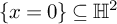 as separating space in the first example. A calculation yields that the Hilbert transform in the sense of the manifold model is

where g is the class
$\pm [a_{i, j}]_{i,j}$
 . This multiplier can be related to the other two models. Indeed, for the Hilbert space model, it is possible to construct a metrically proper
$1$
. This multiplier can be related to the other two models. Indeed, for the Hilbert space model, it is possible to construct a metrically proper
$1$
 -cocycle
$\beta : \mathrm {PSL}_2(\mathbb {K}) \to \mathcal {H}$
-cocycle
$\beta : \mathrm {PSL}_2(\mathbb {K}) \to \mathcal {H}$
 into an infinite-dimensional Hilbert space
$\mathcal {H}$
into an infinite-dimensional Hilbert space
$\mathcal {H}$
 and choose a unit vector
$u \in \mathcal {H}$
and choose a unit vector
$u \in \mathcal {H}$
 such that
$m(g) = \mathrm {sgn} \langle \beta (g), u \rangle $
such that
$m(g) = \mathrm {sgn} \langle \beta (g), u \rangle $
 , see [Reference Erven and Falkowski27, Reference Cherix, Cowling, Jolissaint, Julg and Valette13]. While the group
$\mathrm {PSL}_2(\mathbb {R})$
, see [Reference Erven and Falkowski27, Reference Cherix, Cowling, Jolissaint, Julg and Valette13]. While the group
$\mathrm {PSL}_2(\mathbb {R})$
 is continuous, and thus it is unable to act on trees in an interesting way, the tree model interpretation is indeed available for the restriction of (1.7) to
$\mathrm {PSL}_2(\mathbb {Z})$
is continuous, and thus it is unable to act on trees in an interesting way, the tree model interpretation is indeed available for the restriction of (1.7) to
$\mathrm {PSL}_2(\mathbb {Z})$
 . The key observation is that

This free-product decomposition yields an action of
$\mathrm {PSL}_2(\mathbb {Z})$
 on its Bass-Serre tree with respect to which the multiplier
$m{|}_{\mathrm {PSL}_2(\mathbb {Z})}$
on its Bass-Serre tree with respect to which the multiplier
$m{|}_{\mathrm {PSL}_2(\mathbb {Z})}$
 can be recovered, see Figure 10.
For the complex case, the separating subspace is given by the
$2$
 -dimensional geodesic submanifold
$\{ x = 0 \} \subseteq \mathbb {H}^2$
-dimensional geodesic submanifold
$\{ x = 0 \} \subseteq \mathbb {H}^2$
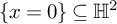 , which readily gives that

where
$x_0 = (0,1) \in \mathbb {C} \times \mathbb {R}_+$
 ,
$p(z,r) = z$
,
$p(z,r) = z$
 and
$g = \pm [z_{i, j}]_{i,j}$
and
$g = \pm [z_{i, j}]_{i,j}$
 . In this case, the relationship with the other two models is more involved. Nevertheless, it is still possible to describe the multiplier (1.8) above in terms of proper infinite-dimensional
$1$
. In this case, the relationship with the other two models is more involved. Nevertheless, it is still possible to describe the multiplier (1.8) above in terms of proper infinite-dimensional
$1$
 -cocycles with respect to a natural direction u. For the tree model the situation is a lot more contentious. Indeed, let
$\mathcal {O}_{-d}$
-cocycles with respect to a natural direction u. For the tree model the situation is a lot more contentious. Indeed, let
$\mathcal {O}_{-d}$
 be the ring of integers of the algebraic field
$\mathbb {Q}(\sqrt {-d})$
be the ring of integers of the algebraic field
$\mathbb {Q}(\sqrt {-d})$
 , where d is a square-free integer. The lattices
$\mathrm {PSL}_2(\mathcal {O}_{-d}) \subseteq \mathrm {PSL}_2(\mathbb {C})$
, where d is a square-free integer. The lattices
$\mathrm {PSL}_2(\mathcal {O}_{-d}) \subseteq \mathrm {PSL}_2(\mathbb {C})$
 are the Bianchi groups. It is known that all of them except for
$d = 3$
are the Bianchi groups. It is known that all of them except for
$d = 3$
 admit nontrivial actions on trees, see [Reference Frohman and Fine29]. For instance, when
$d=1$
admit nontrivial actions on trees, see [Reference Frohman and Fine29]. For instance, when
$d=1$
 ,
$\mathcal {O}_{-1}$
,
$\mathcal {O}_{-1}$
 is the ring of Gaussian integers
$\mathbb {Z}[i]$
is the ring of Gaussian integers
$\mathbb {Z}[i]$
 . In this case, the following rather intricate free product decomposition is known:

where
$S_n$
 are the permutation groups,
$A_n$
are the permutation groups,
$A_n$
 are the alternating groups and V is the Klein
$4$
are the alternating groups and V is the Klein
$4$
 group, see [Reference Frohman and Fine29, Theorem 2.1. (i)]. It is possible that m, when restricted to
$\mathrm {PSL}_2(\mathcal {O}_{-d})$
group, see [Reference Frohman and Fine29, Theorem 2.1. (i)]. It is possible that m, when restricted to
$\mathrm {PSL}_2(\mathcal {O}_{-d})$
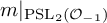
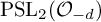 , may have an expression in terms of a nontrivial action on a tree. Nevertheless, the complexity of the amalgamated free product decompositions obtained makes it a difficult approach to work with. On the other hand, the strength of our characterization in Theorem A allows us to prove the boundedness of
$m{|}_{\mathrm {PSL}_2(\mathcal {O}_{-1})}$
, may have an expression in terms of a nontrivial action on a tree. Nevertheless, the complexity of the amalgamated free product decompositions obtained makes it a difficult approach to work with. On the other hand, the strength of our characterization in Theorem A allows us to prove the boundedness of
$m{|}_{\mathrm {PSL}_2(\mathcal {O}_{-1})}$
 directly.
Theorem E. Let
$\mathrm {G} = \mathrm {PSL}_2(\mathcal {O}_{-1}) \subseteq \mathrm {PSL}_2(\mathbb {C})$
 and
$m: \mathrm {PSL}_2(\mathcal {O}_{-1}) \to \mathbb {C}$
and
$m: \mathrm {PSL}_2(\mathcal {O}_{-1}) \to \mathbb {C}$
 be the function given by

Then,
$T_m:L_p(\mathcal {L} \mathrm {G}) \to L_p(\mathcal {L} \mathrm {G})$
 is bounded for every
$1 < p <\infty $
is bounded for every
$1 < p <\infty $
 with the bound in Theorem A.
Foreword: In the first released version of this text we left two natural problems open. The first was whether
$m{|}_\Gamma $
 is
$L_p$
is
$L_p$
 -bounded for lattices
$\Gamma $
-bounded for lattices
$\Gamma $
 other than
$\mathrm {PSL}_2(\mathcal {O}_{-1})$
other than
$\mathrm {PSL}_2(\mathcal {O}_{-1})$
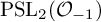 . In the years following its release, significant progress toward a positive answer has been made by Jorge Pérez García [Reference Pérez García73]. The second problem, originally highlighted as Problem A, asked if the multipliers (1.7) and (1.8) are
$L_p$
. In the years following its release, significant progress toward a positive answer has been made by Jorge Pérez García [Reference Pérez García73]. The second problem, originally highlighted as Problem A, asked if the multipliers (1.7) and (1.8) are
$L_p$
 -bounded over the whole Lie group. This has been answered in the negative by the second-named author, together with de la Salle and Tablate [Reference Parcet, de la Salle and Tablate64], via an extension of Fefferman’s ball multiplier construction in the context of Schur multipliers.
2 Cotlar identities and multipliers
Noncommutative integration. Throughout this text we will use liberally noncommutative integration theory and the theory of noncommutative
$L_p$
 -spaces. Let
$\mathcal {M} \subseteq \mathcal {B}(\mathcal {H})$
-spaces. Let
$\mathcal {M} \subseteq \mathcal {B}(\mathcal {H})$
 be a
von Neumann algebra admitting a normal semifinite and faithful tracial weight
$\tau : \mathcal {M}_+ \to [0,\infty ]$
be a
von Neumann algebra admitting a normal semifinite and faithful tracial weight
$\tau : \mathcal {M}_+ \to [0,\infty ]$
 that we will henceforth just refer to as a n.s.f. trace. It is possible to construct the noncommutative
$L_p$
that we will henceforth just refer to as a n.s.f. trace. It is possible to construct the noncommutative
$L_p$
 -spaces associated to
$(\mathcal {M},\tau )$
-spaces associated to
$(\mathcal {M},\tau )$
 as the subset of
$\tau $
as the subset of
$\tau $
 -measurable operators
$L_p(\mathcal {M},\tau ) \subseteq L_0(\mathcal {M},\tau )$
-measurable operators
$L_p(\mathcal {M},\tau ) \subseteq L_0(\mathcal {M},\tau )$
 satisfying that

This theory, which goes back all the way to Dixmier and Segal [Reference Dixmier24, Reference Segal78], is already well understood and the interested reader can consult [Reference Terp84, Reference Pisier and Xu72, Reference Goldstein and Labuschagne32].
Let
$\mathrm {G}$
 be a locally compact group that we will throughout the text assume to be second countable, and let
$L_2(\mathrm {G})$
be a locally compact group that we will throughout the text assume to be second countable, and let
$L_2(\mathrm {G})$
 be its
$L_2$
be its
$L_2$
 -space with respect to the left Haar measure
$\mu $
-space with respect to the left Haar measure
$\mu $
 [Reference Folland28]. As usual, we will denote by
$\lambda : \mathrm {G} \to \mathcal {U}(L_2 (\mathrm {G}))$
[Reference Folland28]. As usual, we will denote by
$\lambda : \mathrm {G} \to \mathcal {U}(L_2 (\mathrm {G}))$
 the left regular representation, which is the unitary representation
$g \mapsto \lambda _g$
the left regular representation, which is the unitary representation
$g \mapsto \lambda _g$
 that acts by sending
$\xi (h)$
that acts by sending
$\xi (h)$
 to
$\xi (g^{-1} h)$
to
$\xi (g^{-1} h)$
 . The left regular von Neumann algebra
$\mathcal {L} \mathrm {G} \subseteq \mathcal {B}(L_2 (\mathrm {G}))$
. The left regular von Neumann algebra
$\mathcal {L} \mathrm {G} \subseteq \mathcal {B}(L_2 (\mathrm {G}))$
 of
$\mathrm {G}$
of
$\mathrm {G}$
 is given by

This von Neumann algebra admits a normal, semifinite and faithful weight
$\tau : \mathcal {L} \mathrm {G}_+ \to [0,\infty ]$
 that satisfies the Plancherel identity, meaning that
$\varphi \mapsto \lambda (\varphi )$
that satisfies the Plancherel identity, meaning that
$\varphi \mapsto \lambda (\varphi )$
 extends to a unitary isometry from
$L_2(\mathrm {G})$
extends to a unitary isometry from
$L_2(\mathrm {G})$
 to the Gelfand-Neumark-Segal space
$L_2(\mathcal {L} \mathrm {G};\tau )$
to the Gelfand-Neumark-Segal space
$L_2(\mathcal {L} \mathrm {G};\tau )$
 . This weight is usually referred to as the Plancherel weight [Reference Pedersen67, Chapter 7]. The weight
$\tau $
. This weight is usually referred to as the Plancherel weight [Reference Pedersen67, Chapter 7]. The weight
$\tau $
 is a n.s.f. trace precisely when
$\mathrm {G}$
is a n.s.f. trace precisely when
$\mathrm {G}$
 is unimodular. Thus, we will work in the natural setting of unimodular groups and refer to
$\tau $
is unimodular. Thus, we will work in the natural setting of unimodular groups and refer to
$\tau $
 as the Plancherel trace. In this context, the Plancherel trace is given by

We will denote the noncommutative
$L_p$
 -spaces associated to
$\tau $
-spaces associated to
$\tau $
 simply by
$L_p(\mathcal {L} \mathrm {G})$
simply by
$L_p(\mathcal {L} \mathrm {G})$
 . By analogy with the classical Fourier transform, we will denote by
$\widehat {f}(g)$
. By analogy with the classical Fourier transform, we will denote by
$\widehat {f}(g)$
 the value
$\tau (\lambda _g^\ast f)$
the value
$\tau (\lambda _g^\ast f)$
 , which is well-defined whenever
$f \in L_1(\mathcal {L} \mathrm {G})$
, which is well-defined whenever
$f \in L_1(\mathcal {L} \mathrm {G})$
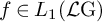 . It is also worth noticing that, by Plancherel’s theorem, the map
$f \mapsto \widehat {f}$
. It is also worth noticing that, by Plancherel’s theorem, the map
$f \mapsto \widehat {f}$
 is well-defined for any
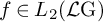
$f \in L_2(\mathcal {L} \mathrm {G})$
is well-defined for any
$f \in L_2(\mathcal {L} \mathrm {G})$
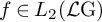 . In fact, we have that
$f \in L_2(\mathcal {L} \mathrm {G})$
. In fact, we have that
$f \in L_2(\mathcal {L} \mathrm {G})$
 can be expressed as

where the integral on the right-hand side converges in the
$L_2$
 norm.
norm.
Conditional expectations. Let
$\mathcal {N} \subseteq \mathcal {M}$
 be a von Neumann subalgebra of
$\mathcal {M}$
be a von Neumann subalgebra of
$\mathcal {M}$
 , that is a
$\ast $
, that is a
$\ast $
 -subalgebra that is also ultraweakly closed. If
$\tau $
-subalgebra that is also ultraweakly closed. If
$\tau $
 is a n.s.f. trace over
$\mathcal {M}$
is a n.s.f. trace over
$\mathcal {M}$
 and
$\tau {|}_{\mathcal {N}}$
and
$\tau {|}_{\mathcal {N}}$
 is still semifinite, then it is easy to see that the inclusion
$\iota : L_1(\mathcal {N}) \hookrightarrow L_1(\mathcal {M})$
is still semifinite, then it is easy to see that the inclusion
$\iota : L_1(\mathcal {N}) \hookrightarrow L_1(\mathcal {M})$
 is isometric and its dual map is a trace preserving and normal (i.e., ultraweakly continuous) conditional expectation
$\mathbb {E}: \mathcal {M} \to \mathcal {N} \subseteq \mathcal {M}$
is isometric and its dual map is a trace preserving and normal (i.e., ultraweakly continuous) conditional expectation
$\mathbb {E}: \mathcal {M} \to \mathcal {N} \subseteq \mathcal {M}$
 . By conditional expectation we mean a unital and completely positive map such that
$\mathbb {E}{|}_{\mathcal {N}} = \mathrm {id}_{\mathcal {N}}$
. By conditional expectation we mean a unital and completely positive map such that
$\mathbb {E}{|}_{\mathcal {N}} = \mathrm {id}_{\mathcal {N}}$
 . Recall that conditional expectations satisfy that
$\mathbb {E} \circ \mathbb {E} = \mathbb {E}$
. Recall that conditional expectations satisfy that
$\mathbb {E} \circ \mathbb {E} = \mathbb {E}$
 and that, by Tomiyama’s Theorem, see [Reference Brown and Ozawa7, Theorem 1.5.10],
$\mathbb {E}$
and that, by Tomiyama’s Theorem, see [Reference Brown and Ozawa7, Theorem 1.5.10],
$\mathbb {E}$
 is automatically
$\mathcal {N}$
is automatically
$\mathcal {N}$
 -bimodular.
Let
$\mathrm {G}_0 \subseteq \mathrm {G}$
 be two groups such that
$\mathrm {G}_0$
be two groups such that
$\mathrm {G}_0$
 is open inside
$\mathrm {G}$
is open inside
$\mathrm {G}$
 . Then
$\mathrm {G}_0$
. Then
$\mathrm {G}_0$
 is unimodular if
$\mathrm {G}$
is unimodular if
$\mathrm {G}$
 is. Furthermore, the Plancherel trace
$\tau _{\mathrm {G}_0}$
is. Furthermore, the Plancherel trace
$\tau _{\mathrm {G}_0}$
 of
$\mathcal {L} \mathrm {G}_0$
of
$\mathcal {L} \mathrm {G}_0$
 coincides with the Plancherel trace of
$\mathcal {L} \mathrm {G}$
coincides with the Plancherel trace of
$\mathcal {L} \mathrm {G}$
 restricted to
$\mathcal {L} \mathrm {G}_0$
restricted to
$\mathcal {L} \mathrm {G}_0$
 . Therefore there is a normal and trace-preserving conditional expectation
$\mathbb {E}: \mathcal {L} \mathrm {G} \to \mathcal {L} \mathrm {G}_0 \subseteq \mathcal {L} \mathrm {G}$
. Therefore there is a normal and trace-preserving conditional expectation
$\mathbb {E}: \mathcal {L} \mathrm {G} \to \mathcal {L} \mathrm {G}_0 \subseteq \mathcal {L} \mathrm {G}$
 that is given by the Fourier multiplier associated to
${\mathbf {1}}_{\mathrm {G}_0}$
that is given by the Fourier multiplier associated to
${\mathbf {1}}_{\mathrm {G}_0}$
 , i.e.,

The fact that
$\mathbb {E}$
 is trace preserving allows us to extend
$\mathbb {E}$
is trace preserving allows us to extend
$\mathbb {E}$
 as a contraction to all the
$L_p$
as a contraction to all the
$L_p$
 -spaces
$1\leq p \leq \infty $
-spaces
$1\leq p \leq \infty $
 ,
$\mathbb {E}:L_p(\mathcal {L} \mathrm {G}) \to L_p(\mathcal {L} \mathrm {G}_0) \subseteq L_p(\mathcal {L} \mathrm {G})$
,
$\mathbb {E}:L_p(\mathcal {L} \mathrm {G}) \to L_p(\mathcal {L} \mathrm {G}_0) \subseteq L_p(\mathcal {L} \mathrm {G})$
 .
.
Noncommutative Cotlar identities. Most of this section up until the closed-formula characterization of the Cotlar identity in the proof of Theorem A follows closely the results obtained by Mei and Ricard and it is included here for the sake of completeness.
Definition 2.1 [Reference Mei and Ricard55, from Proposition 3.2(iv)]
Let
$\mathcal {M}$
 ,
$\mathcal {N}$
,
$\mathcal {N}$
 be as above,
$\mathbb {E}: \mathcal {M} \to \mathcal {N}$
be as above,
$\mathbb {E}: \mathcal {M} \to \mathcal {N}$
 be the conditional expectation and let
$H:L_2(\mathcal {M}) \to L_2(\mathcal {M})$
be the conditional expectation and let
$H:L_2(\mathcal {M}) \to L_2(\mathcal {M})$
 be a bounded operator
-
(i) H satisfies the (non-relative) Cotlar identity if
(Cotlarnr) $$\begin{align} H(f) \, H(f)^\ast \, = \, H \big( f \, H(f)^\ast \big) + H \big( f \, H(f)^\ast \big)^\ast - H \big( H(f f^\ast) \big)^\ast, \end{align}$$for every $f \in \mathcal {M} \cap L_2(\mathcal {M})$
.
-
(ii) H is said to satisfy the Cotlar identity (relative to $\mathcal {N}$
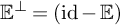
) if (Cotlar𝔼⊥) $$\begin{align} \mathbb{E}^\perp \big[ H(f) \, H(f)^\ast \big] \, = \, \mathbb{E}^\perp \left[ H \big( f \, H(f)^\ast \big) + H \big( f \, H(f)^\ast \big)^\ast - H \big( H(f f^\ast)^\ast \big) \right], \end{align}$$for every $f \in L_2(\mathcal {M}) \cap \mathcal {M}$
, where
$\mathbb {E}^\perp = (\mathrm {id} - \mathbb {E})$
.





We are assuming that H is bounded in
$L_2(\mathcal {M})$
 a priori; this is not a restrictive imposition since it holds trivially in the case of Fourier multipliers. Observe as well that, although both Cotlar identities require applying H to products of functions that therefore may not be in
$L_2(\mathcal {M})$
a priori; this is not a restrictive imposition since it holds trivially in the case of Fourier multipliers. Observe as well that, although both Cotlar identities require applying H to products of functions that therefore may not be in
$L_2(\mathcal {M})$
 , the fact that
$f \in L_2(\mathcal {M}) \cap \mathcal {M}$
, the fact that
$f \in L_2(\mathcal {M}) \cap \mathcal {M}$
 and that
$L_2(\mathcal {M})$
and that
$L_2(\mathcal {M})$
 is stable by multiplications by
$\mathcal {M}$
is stable by multiplications by
$\mathcal {M}$
 makes both equations meaningful.
We will need the following lemma. Notice that if
$H: L_2(\mathcal {M}) \to L_2(\mathcal {M})$
 is left
$\mathcal {N}$
is left
$\mathcal {N}$
 -modular, then its restriction to
$L_2(\mathcal {N})$
-modular, then its restriction to
$L_2(\mathcal {N})$
 composed with the expectation
$\mathbb {E}:L_2(\mathcal {M}) \to L_2(\mathcal {N})$
composed with the expectation
$\mathbb {E}:L_2(\mathcal {M}) \to L_2(\mathcal {N})$
 gives a map

that is both bounded with norm equal to that of H and and left
$\mathcal {N}$
 -modular. But all left
$\mathcal {N}$
-modular. But all left
$\mathcal {N}$
 -modular maps in
$L_2(\mathcal {N})$
-modular maps in
$L_2(\mathcal {N})$
 are right multiplicators by an element in
$\mathcal {N}$
are right multiplicators by an element in
$\mathcal {N}$
 of norm equal to the operator norm. As such,
$\mathbb {E} \, H \, {|}_{L_2(\mathcal {N}) \cap L_p(N)}$
of norm equal to the operator norm. As such,
$\mathbb {E} \, H \, {|}_{L_2(\mathcal {N}) \cap L_p(N)}$
 extends to a bounded operator in
$L_p(\mathcal {N})$
extends to a bounded operator in
$L_p(\mathcal {N})$
 and
and

With this observation in hand, we can proceed to prove the following lemma, which is analogous to [Reference Mei and Ricard55, Proposition 3.4], but in the setting of general operators.
Lemma 2.2. Let
$\mathcal {M}$
 ,
$\mathcal {N}$
,
$\mathcal {N}$
 and
$\mathbb {E}$
and
$\mathbb {E}$
 be as above and let
$H:L_2(\mathcal {M}) \to L_2(\mathcal {M})$
be as above and let
$H:L_2(\mathcal {M}) \to L_2(\mathcal {M})$
 be a bounded and left
$\mathcal {N}$
be a bounded and left
$\mathcal {N}$
 -modular map. For every
$f \in L_2(\mathcal {M}) \cap \mathcal {M}$
-modular map. For every
$f \in L_2(\mathcal {M}) \cap \mathcal {M}$
 , it holds that

Furthermore, if
$\mathbb {E} H = H \mathbb {E}$
 , we have that for every
$1 \leq p \leq \infty $
, we have that for every
$1 \leq p \leq \infty $


Proof. All of the points are elementary. For (2.3) first notice that every state of
$\mathcal {N}$
 is of the form
$f \mapsto \tau ( \delta \, f)$
is of the form
$f \mapsto \tau ( \delta \, f)$
 , where
$\delta $
, where
$\delta $
 is a positive element of norm
$1$
is a positive element of norm
$1$
 in the space
$L_1(\mathcal {N})$
in the space
$L_1(\mathcal {N})$
 . Decomposing it as
$\delta = \delta ^{\frac {1}{2}} \delta ^{\frac {1}{2}}$
. Decomposing it as
$\delta = \delta ^{\frac {1}{2}} \delta ^{\frac {1}{2}}$
 gives
gives

Since this is true for every state, the operator inequality (2.3) holds.
For (2.4) we use that
$\mathbb {E} H = H \mathbb {E}$
 to rewrite
$\mathbb {E} \left [ H \big (f \, H(f)^\ast \big ) \right ]$
to rewrite
$\mathbb {E} \left [ H \big (f \, H(f)^\ast \big ) \right ]$
 as
$(\mathbb {E} H \mathbb {E}) \circ \mathbb {E} \left [ \big (f \, H(f)^\ast \big ) \right ]$
as
$(\mathbb {E} H \mathbb {E}) \circ \mathbb {E} \left [ \big (f \, H(f)^\ast \big ) \right ]$
 . The operator norm on
$\mathbb {E} H \mathbb {E}: L_p(\mathcal {M}) \to L_p(\mathcal {M})$
. The operator norm on
$\mathbb {E} H \mathbb {E}: L_p(\mathcal {M}) \to L_p(\mathcal {M})$
 is bounded by that of
$\mathbb {E} H {|}_{L_p(\mathcal {N})}: L_p(\mathcal {N}) \to L_p(\mathcal {N})$
is bounded by that of
$\mathbb {E} H {|}_{L_p(\mathcal {N})}: L_p(\mathcal {N}) \to L_p(\mathcal {N})$
 , which is bounded by the norm of H by (2.2). To estimate the term
$\mathbb {E} \left [ \big (f \, H(f)^\ast \big ) \right ]$
, which is bounded by the norm of H by (2.2). To estimate the term
$\mathbb {E} \left [ \big (f \, H(f)^\ast \big ) \right ]$
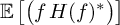 we will use the following version of Hölder’s inequality [Reference Junge41, Inequality (2.1)]

with
$r = s = 2p$
 and
$g = H(f)$
and
$g = H(f)$
 to obtain that

Applying the inequality in (2.3) gives the result. Identity (2.5) follows immediately after using two times the fact that H and
$\mathbb {E}$
 commute and that
$\mathbb {E} H \mathbb {E}$
commute and that
$\mathbb {E} H \mathbb {E}$
 has a norm in
$L_p$
has a norm in
$L_p$
 bounded by the norm in
$L_2$
bounded by the norm in
$L_2$
 of H by (2.2).
We can now prove the following extrapolation result, which generalizes [Reference Mei and Ricard55, Theorem 3.5] to the setting of general operators.
Proposition 2.3. Let
$\mathcal {N} \subseteq \mathcal {M}$
 be as before and let
$H:L_2(\mathcal {M}) \to L_2(\mathcal {M})$
be as before and let
$H:L_2(\mathcal {M}) \to L_2(\mathcal {M})$
 be a left
$\mathcal {N}$
be a left
$\mathcal {N}$
 -modular operator commuting with
$\mathbb {E}: \mathcal {M} \to \mathcal {N}$
-modular operator commuting with
$\mathbb {E}: \mathcal {M} \to \mathcal {N}$
 . If H satisfies (Cotlar𝔼
⊥) then
$\forall \, 2 \leq p < \infty $
. If H satisfies (Cotlar𝔼
⊥) then
$\forall \, 2 \leq p < \infty $


Similarly, if
$H:L_2(\mathcal {M}) \to L_2(\mathcal {M})$
 is a general bounded linear map that satisfies the non-relative Cotlar identity (Cotlarnr), then the same extrapolation inequality (2.6) holds.
Proof. First, let us denote the operator norm on
$L_p$
 of H by
$c_p := \big \| H: L_p(\mathcal {M}) \to L_p(\mathcal {M})\big \|$
of H by
$c_p := \big \| H: L_p(\mathcal {M}) \to L_p(\mathcal {M})\big \|$
 . We are going to proceed by induction, assuming that
$c_p < \infty $
. We are going to proceed by induction, assuming that
$c_p < \infty $
 to prove that
$c_{2p} < \infty $
to prove that
$c_{2p} < \infty $
 . Choose
$f \in \mathcal {M} \cap L_2(\mathcal {M})$
. Choose
$f \in \mathcal {M} \cap L_2(\mathcal {M})$
 with
$\| f \|_{2p} \leq 1$
with
$\| f \|_{2p} \leq 1$
 and notice that


We have used (Cotlar𝔼
⊥) in the second term of the sum of (2.7) and estimate (2.3) of Lemma 2.2 in the first. To pass from (2.8) to (2.9) we have used the other two identities of Lemma 2.2. Notice that (2.9) is a quadratic inequality of the form
$0 \leq -t^2 + 2 c_p \, t + c_p^2 + 4 \, c_2^2$
 , where
$t = \| H(f)\|_{2p}$
, where
$t = \| H(f)\|_{2p}$
 . Since the leading term is negative, this implies a bound of
$\|H(f)\|_{2p}$
. Since the leading term is negative, this implies a bound of
$\|H(f)\|_{2p}$
 in terms of
$c_p$
in terms of
$c_p$
 and
$c_2$
and
$c_2$
 only. Taking supremum over f and using the norm density of
$\mathcal {M} \cap L_{2}(\mathcal {M})$
only. Taking supremum over f and using the norm density of
$\mathcal {M} \cap L_{2}(\mathcal {M})$
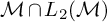 in
$L_{2p}(\mathcal {M})$
in
$L_{2p}(\mathcal {M})$
 implies that
$c_{2p}$
implies that
$c_{2p}$
 is finite. More explicitly, setting
$a_p = c_p / c_2$
is finite. More explicitly, setting
$a_p = c_p / c_2$
 gives the recursive inequality

Adding
$a_{2p}^2$
 to both sides in order to complete squares gives

After taking square roots and recursively applying the inequality above, the following is obtained

This, together with Marcinkiewicz interpolation for intermediate values of p, gives the desired inequality. The non-relative case works similarly, but the
$4$
 extra terms that give
$4 \, c_2^2$
extra terms that give
$4 \, c_2^2$
 in the right-hand side of inequality (2.9) do not appear, which only affects the absolute constant C in the final inequality.
Our source of examples for the extrapolation theorem above is taken when
$\mathcal {M} = \mathcal {L} \mathrm {G}$
 and
$H=T_m$
and
$H=T_m$
 is a Fourier multiplier. We will work with Cotlar identities relative to subalgebras induced by subgroups
$\mathrm {G}_0 \subseteq \mathrm {G}$
is a Fourier multiplier. We will work with Cotlar identities relative to subalgebras induced by subgroups
$\mathrm {G}_0 \subseteq \mathrm {G}$
 . In that setting it holds that there is a normal and trace-preserving conditional expectation
$\mathbb {E}: \mathcal {L} \mathrm {G} \to \mathcal {L} \mathrm {G}_0$
. In that setting it holds that there is a normal and trace-preserving conditional expectation
$\mathbb {E}: \mathcal {L} \mathrm {G} \to \mathcal {L} \mathrm {G}_0$
 if and only if
$\mathrm {G}_0 \subseteq \mathrm {G}$
if and only if
$\mathrm {G}_0 \subseteq \mathrm {G}$
 is open. Thus, our relative Cotlar identities would be taken only with respect to open subgroups. In general, given a group
$\mathrm {G}$
is open. Thus, our relative Cotlar identities would be taken only with respect to open subgroups. In general, given a group
$\mathrm {G}$
 , when speaking about the Cotlar identity for a multiplier
$T_m$
, when speaking about the Cotlar identity for a multiplier
$T_m$
 – without specifying any subgroup – we will mean, that it satisfies the non-relative Cotlar identity (Cotlarnr) when the group
$\mathrm {G}$
– without specifying any subgroup – we will mean, that it satisfies the non-relative Cotlar identity (Cotlarnr) when the group
$\mathrm {G}$
 is continuous i.e.
$\mu (\{e\}) = 0$
is continuous i.e.
$\mu (\{e\}) = 0$
 , while in the discrete case
$\mu (\{e\}) \neq 0$
, while in the discrete case
$\mu (\{e\}) \neq 0$
 , we will instead mean that it satisfies (Cotlar𝔼
⊥) with respect to the subgroup
$\{e\}$
, we will instead mean that it satisfies (Cotlar𝔼
⊥) with respect to the subgroup
$\{e\}$
 .
.
We are now going to prove the equivalence between Cotlar’s identity (Cotlar𝔼 ⊥) and the closed formula in Theorem A.
Theorem 2.4. Let
$\mathrm {G}_0 \subseteq \mathrm {G}$
 be an open subgroup of
$\mathrm {G}$
be an open subgroup of
$\mathrm {G}$
 and
$m: \mathrm {G} \to \mathbb {C}$
and
$m: \mathrm {G} \to \mathbb {C}$
 be a bounded function. The following properties are equivalent:



Proof. Expanding (Cotlar𝔼
⊥) for
$T_m$
 gives
gives

Now, elementary computations yield that

where
$\widehat {f}$
 is given as in (2.1). This in turn implies, using the Plancherel theorem, that

Obviously, if the factor
$G_g(h) = ( m(gh) - m(g) ) \, ( \overline {m(h) - m(g^{-1})} )$
 is equal to
$0$
is equal to
$0$
 so is the above integral and therefore (Cotlar𝔼
⊥) holds. The reciprocal is immediate in the case of discrete groups. Indeed, choose any
$h_0 \in \mathrm {G}$
so is the above integral and therefore (Cotlar𝔼
⊥) holds. The reciprocal is immediate in the case of discrete groups. Indeed, choose any
$h_0 \in \mathrm {G}$
 and assume that
$g \in \mathrm {G} \setminus \mathrm {G}_0$
and assume that
$g \in \mathrm {G} \setminus \mathrm {G}_0$
 is fixed. Pick
$\widehat {f} = \delta _{h_0} + \delta _{g h_0}$
is fixed. Pick
$\widehat {f} = \delta _{h_0} + \delta _{g h_0}$
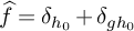 . In order to evaluate the integral, notice that

The term
$\delta _{h=h_0}$
 in the above sum gives
${G_g(h_0)}$
in the above sum gives
${G_g(h_0)}$
 in the integral. The term in which
$g^2=e$
in the integral. The term in which
$g^2=e$
 and
$h = g h_0$
and
$h = g h_0$
 gives
$\overline {G_g(h_0)}$
gives
$\overline {G_g(h_0)}$
 . Therefore,
$\operatorname {Re}\{ G_g(h)\}=0$
. Therefore,
$\operatorname {Re}\{ G_g(h)\}=0$
 for any
$h \in \mathrm {G}$
for any
$h \in \mathrm {G}$
 . The imaginary part is similarly shown to be
$0$
. The imaginary part is similarly shown to be
$0$
 . In the case of a continuous group
$\mathrm {G}$
. In the case of a continuous group
$\mathrm {G}$
 it is necessary to replace
$\delta _{h_0}$
it is necessary to replace
$\delta _{h_0}$
 with an approximation of the unit.
Remark 2.5. Notice that Theorem 2.4 works similarly in the non-relative case. In that case it holds that
$T_m$
 has the (Cotlarnr) if and only if m satisfies the identity
$( m(g^{-1} ) - m(h) ) \, ( m(gh) - m(g) ) = 0$
has the (Cotlarnr) if and only if m satisfies the identity
$( m(g^{-1} ) - m(h) ) \, ( m(gh) - m(g) ) = 0$
 for almost every
$g, h \in \mathrm {G}$
for almost every
$g, h \in \mathrm {G}$
 .
.
With all that at hand we are ready to prove Theorem A.
Proof of Theorem A
Since
$\mathrm {G}_0$
 is closed, we have two situations, either it is open or of empty interior. In the first case, we have that
$\mu (\mathrm {G}_0)> 0$
is closed, we have two situations, either it is open or of empty interior. In the first case, we have that
$\mu (\mathrm {G}_0)> 0$
 and we have that the formula in (ii) is equivalent to (Cotlar𝔼
⊥) by Theorem 2.4. Observe that, if m is left-
$\mathrm {G}_0$
and we have that the formula in (ii) is equivalent to (Cotlar𝔼
⊥) by Theorem 2.4. Observe that, if m is left-
$\mathrm {G}_0$
 invariant, then
$T_m$
invariant, then
$T_m$
 is left
$\mathcal {L} \mathrm {G}_0$
is left
$\mathcal {L} \mathrm {G}_0$
 -modular. Thus, we can apply Proposition 2.3 to obtain the bound (1.1) for
$p \geq 2$
-modular. Thus, we can apply Proposition 2.3 to obtain the bound (1.1) for
$p \geq 2$
 . Using that, by Plancherel theorem,
$\| T_m:L_2(\mathcal {L} \mathrm {G}) \to L_2(\mathcal {L} \mathrm {G}) \| = \| m \|_\infty $
. Using that, by Plancherel theorem,
$\| T_m:L_2(\mathcal {L} \mathrm {G}) \to L_2(\mathcal {L} \mathrm {G}) \| = \| m \|_\infty $
 we get the result for
$2 \geq p$
we get the result for
$2 \geq p$
 . For
$1 < p < 2$
. For
$1 < p < 2$
 the result follows by standard duality arguments. In the case of
$\mathrm {G}_0$
the result follows by standard duality arguments. In the case of
$\mathrm {G}_0$
 of empty interior the proof follows similarly by using Remark 2.5 and the last assertion of Proposition 2.3.
Remark 2.6. Let
$\alpha : \mathcal {N} \to \mathcal {N}$
 be a normal and trace-preserving
$\ast $
be a normal and trace-preserving
$\ast $
 -homomorphism. It is immediate that both Proposition 2.3 and Lemma 2.2 hold if we change the condition of H being left
$\mathcal {N}$
-homomorphism. It is immediate that both Proposition 2.3 and Lemma 2.2 hold if we change the condition of H being left
$\mathcal {N}$
 -modular by that of being left
$\mathcal {N}$
-modular by that of being left
$\mathcal {N}$
 -modular relative to
$\alpha $
-modular relative to
$\alpha $
 , i.e.,

In the case of multipliers this easy observation has deep consequences. For instance, let
$\chi : \mathrm {G}_0 \to \mathbb {T}$
 be a (multiplicative) character. It is a straightforward consequence of Fell’s absorption principle that the map
$\lambda _g \mapsto \chi (g) \, \lambda _g$
be a (multiplicative) character. It is a straightforward consequence of Fell’s absorption principle that the map
$\lambda _g \mapsto \chi (g) \, \lambda _g$
 induces a normal and trace-preserving
$\ast $
induces a normal and trace-preserving
$\ast $
 -automorphism
$\alpha _\chi : \mathcal {L} \mathrm {G}_0 \to \mathcal {L} \mathrm {G}_0$
-automorphism
$\alpha _\chi : \mathcal {L} \mathrm {G}_0 \to \mathcal {L} \mathrm {G}_0$
 . Let
$H = T_m$
. Let
$H = T_m$
 be a Fourier multiplier on
$\mathcal {L} \mathrm {G}$
be a Fourier multiplier on
$\mathcal {L} \mathrm {G}$
 . We have that it is left
$\mathcal {L} \mathrm {G}_0$
. We have that it is left
$\mathcal {L} \mathrm {G}_0$
 -modular with respect to
$\alpha _\chi $
-modular with respect to
$\alpha _\chi $
 , i.e.,
$H(f \, g) = \alpha _\chi (f) \, H(g)$
, i.e.,
$H(f \, g) = \alpha _\chi (f) \, H(g)$
 , for every
$f \in \mathcal {N}$
, for every
$f \in \mathcal {N}$
 and
$g \in L_2(\mathcal {M}) \cap \mathcal {M}$
and
$g \in L_2(\mathcal {M}) \cap \mathcal {M}$
 iff
iff

This is specially useful when
$\mathrm {G}_0$
 is Abelian since, in that case, every function on
$\mathrm {G}_0$
is Abelian since, in that case, every function on
$\mathrm {G}_0$
 can be expressed as a limit of linear combinations of characters by the Fourier transform. This will be exploited in Theorem 5.2. It would also be used in a forthcoming paper of the third-named author.
Tightening the constant. It is known that, on the real line
$\mathrm {G} = \mathbb {R}$
 the operator
$L_p$
the operator
$L_p$
 -norm of the classical Hilbert transform (HT) is given by

see [Reference Pichorides68] or [Reference Grafakos34] for a simplified proof. These constants grow asymptotically like p as
$p \to \infty $
 and like
$1/(p-1)$
and like
$1/(p-1)$
 as
$p \to 1^{+}$
as
$p \to 1^{+}$
 , and those are the growth orders that we conjecture optimal in the noncommutative case as well. An interesting observation, originally made by Gokhberg and Krupnik in the classical case [Reference Gokhberg and Krupnik31] is that Cotlar’s identity on the real line gives the optimal order of growth for the constant in terms of p. Indeed, in the classical case, the fact that
$H^2 = - \mathrm {id}$
, and those are the growth orders that we conjecture optimal in the noncommutative case as well. An interesting observation, originally made by Gokhberg and Krupnik in the classical case [Reference Gokhberg and Krupnik31] is that Cotlar’s identity on the real line gives the optimal order of growth for the constant in terms of p. Indeed, in the classical case, the fact that
$H^2 = - \mathrm {id}$
 yields a recurrence relation of the form

instead of (2.10). The lack of a term depending on
$c_p^2$
 gives a decisively smaller bound. Solving the quadratic inequality in (2.12) gives

and that results, after applying duality and interpolation, in the optimal growth order for the constant.
In the noncommutative case, the same type of argument holds for operators
$H: L_2(\mathcal {M}) \to L_2(\mathcal {M})$
 satisfying that
$H \, H_{\mathrm {op}} = -\mathrm {id}$
satisfying that
$H \, H_{\mathrm {op}} = -\mathrm {id}$
 , where
$H_{\mathrm {op}}(f) = H(f^\ast )^\ast $
, where
$H_{\mathrm {op}}(f) = H(f^\ast )^\ast $
 . We have the following improvement over Proposition 2.3.
Proposition 2.7. Let
$\mathcal {N} \subseteq \mathcal {M}$
 and
$H:L_2(\mathcal {M}) \to L_2(\mathcal {M})$
and
$H:L_2(\mathcal {M}) \to L_2(\mathcal {M})$
 be as before and assume H is left
$\mathcal {N}$
be as before and assume H is left
$\mathcal {N}$
 -modular, commutes with
$\mathbb {E}: \mathcal {M} \to \mathcal {N}$
-modular, commutes with
$\mathbb {E}: \mathcal {M} \to \mathcal {N}$
 and satisfies that
$\mathbb {E}^\perp H \, H_{\mathrm {op}} = -\mathbb {E}^\perp $
and satisfies that
$\mathbb {E}^\perp H \, H_{\mathrm {op}} = -\mathbb {E}^\perp $
 . If H satisfies (Cotlar𝔼
⊥), then
. If H satisfies (Cotlar𝔼
⊥), then

The same inequality holds in the non-relative case if
$H \, H_{\mathrm {op}} = -\mathrm {id}$
 .
.
Proof. The proof is immediate once it is noticed that the property
$\mathbb {E}^\perp H \, H_{\mathrm {op}} = -\mathbb {E}^\perp $
 implies that (Cotlar𝔼
⊥) can be rewritten as
implies that (Cotlar𝔼
⊥) can be rewritten as

Applying the same proof as that of Proposition 2.3 gives the recurrence
$c_{2p}^2 \leq 2 \, c_{2 p} \, c_p + 1 + 3 c_2^2$
 . After solving the quadratic inequality, we obtain
$c_{2p} \leq c_p + \sqrt {c_p^2 + \kappa }$
. After solving the quadratic inequality, we obtain
$c_{2p} \leq c_p + \sqrt {c_p^2 + \kappa }$
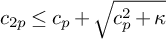 , where
$\kappa = 1 + 3 c_2^2$
, where
$\kappa = 1 + 3 c_2^2$
 . Iterating and applying Marcinkiewicz interpolation gives the bound. The same proof works in the non-relative case.
Observe that if
$H = T_m$
 is a Fourier multiplier, then
$(T_m)_{\mathrm {op}} = T_{\tilde {m}}$
is a Fourier multiplier, then
$(T_m)_{\mathrm {op}} = T_{\tilde {m}}$
 , for
$\widetilde {m}(g) = \overline {m(g^{-1})}$
, for
$\widetilde {m}(g) = \overline {m(g^{-1})}$
 . Thus, we are asking that
$m(g) \, \overline {m(g^{-1})} = -1$
. Thus, we are asking that
$m(g) \, \overline {m(g^{-1})} = -1$
 for every
$g \in \mathrm {G} \setminus \mathrm {G}_0$
for every
$g \in \mathrm {G} \setminus \mathrm {G}_0$
 . Similarly, since in the case of multipliers
$\| \mathbb {E} H({\mathbf {1}}) \|_\infty = \| m \, {\mathbf {1}}_{\mathrm {G}_0} \|_\infty \leq \| m \|_\infty = c_2$
. Similarly, since in the case of multipliers
$\| \mathbb {E} H({\mathbf {1}}) \|_\infty = \| m \, {\mathbf {1}}_{\mathrm {G}_0} \|_\infty \leq \| m \|_\infty = c_2$
 we can simplify the recurrence above assuming
$c_2 = 1$
we can simplify the recurrence above assuming
$c_2 = 1$
 . In particular, we obtain the following corollary.
Corollary 2.8. Let
$\mathrm {G}$
 be a group and let
$m: \mathrm {G} \to \mathbb {C}$
be a group and let
$m: \mathrm {G} \to \mathbb {C}$
 be a function satisfying (Cotla ^r) relative to a closed subgroup
$\mathrm {G}_0 \subseteq \mathrm {G}$
be a function satisfying (Cotla ^r) relative to a closed subgroup
$\mathrm {G}_0 \subseteq \mathrm {G}$
 , and such that m is left
$\mathrm {G}_0$
, and such that m is left
$\mathrm {G}_0$
 -invariant and
$m(g)\overline {m(g^{-1})} = -1$
-invariant and
$m(g)\overline {m(g^{-1})} = -1$
 , for every
$g \in \mathrm {G} \setminus \mathrm {G}_0$
, for every
$g \in \mathrm {G} \setminus \mathrm {G}_0$
 . Then

Both Proposition 2.7 and Corollary 2.8 are still true if one changes the value of
$m(g) \, \overline {m(g^{-1})}$
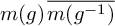 from
$-1$
from
$-1$
 to any other constant independent of g.
Non-Fourier multiplier examples. All of the machinery developed or reviewed in this Section is formulated in a way that works beyond the case of Fourier multipliers. As an illustration, another family of examples comes from Schur multipliers. Indeed, let
$\mathcal {D} \subset \mathcal {B}(\ell _2 \mathbb {Z})$
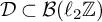 be the finite span of the matrix units
$e_{j \, k}$
be the finite span of the matrix units
$e_{j \, k}$
 . A Schur multiplier is a linear map
$S_m: \mathcal {D} \subseteq \mathcal {B}(\ell _2 \mathbb {Z}) \to \mathcal {B}(\ell _2 \mathbb {Z})$
. A Schur multiplier is a linear map
$S_m: \mathcal {D} \subseteq \mathcal {B}(\ell _2 \mathbb {Z}) \to \mathcal {B}(\ell _2 \mathbb {Z})$
 defined by sending the matrix unit
$e_{j \, k}$
defined by sending the matrix unit
$e_{j \, k}$
 to
$m(j,k) \, e_{j \, k}$
to
$m(j,k) \, e_{j \, k}$
 for some function
$m:\mathbb {Z} \times \mathbb {Z} \to \mathbb {C}$
for some function
$m:\mathbb {Z} \times \mathbb {Z} \to \mathbb {C}$
 – called the symbol of
$S_m$
– called the symbol of
$S_m$
 . Schur multipliers are
$\ell _\infty (\mathbb {Z})$
. Schur multipliers are
$\ell _\infty (\mathbb {Z})$
 -bimodular, with
$\ell _\infty (\mathbb {Z})$
-bimodular, with
$\ell _\infty (\mathbb {Z})$
 sitting inside
$\mathcal {B}(\ell _2 \mathbb {Z})$
sitting inside
$\mathcal {B}(\ell _2 \mathbb {Z})$
 as the diagonal subalgebra. As such, if we take in Theorem 2.3
$\mathcal {M}$
as the diagonal subalgebra. As such, if we take in Theorem 2.3
$\mathcal {M}$
 to be
$\mathcal {B}(\ell _2 \mathbb {Z})$
to be
$\mathcal {B}(\ell _2 \mathbb {Z})$
 and
$\mathcal {N}$
and
$\mathcal {N}$
 to be
$\ell _\infty (\mathbb {Z})$
to be
$\ell _\infty (\mathbb {Z})$
 , we have that any bounded symbol m satisfying (Cotlar𝔼
⊥) extends boundedly to all Schatten classes
$S_p$
, we have that any bounded symbol m satisfying (Cotlar𝔼
⊥) extends boundedly to all Schatten classes
$S_p$
 with
$1 < p < \infty $
with
$1 < p < \infty $
 . The same computations of Theorem 2.4 can be performed in this setting, yielding that

This makes verifying the Cotlar identity for Schur multipliers straightforward. For instance, the triangular truncation
$H = S_m$
 is the Schur multiplier with symbol
$m(j,k) = \mathrm {sgn}(j - k)$
is the Schur multiplier with symbol
$m(j,k) = \mathrm {sgn}(j - k)$
 . It is trivial to verify that it satisfies identity (2.13). Indeed, if
$m(j,k) \neq m(j,\ell )$
. It is trivial to verify that it satisfies identity (2.13). Indeed, if
$m(j,k) \neq m(j,\ell )$
 it is because
$j < \ell $
it is because
$j < \ell $
 and
$j \geq k$
and
$j \geq k$
 or vice–versa. If the first case holds, then
$k \leq j < \ell $
or vice–versa. If the first case holds, then
$k \leq j < \ell $
 , which implies that
$m(\ell ,j) = m(\ell ,k)$
, which implies that
$m(\ell ,j) = m(\ell ,k)$
 . The other case is checked similarly. Since
$H \, H^{\mathrm {op}} = - \mathrm {id}$
. The other case is checked similarly. Since
$H \, H^{\mathrm {op}} = - \mathrm {id}$
 , we recover the sharp bound of the operator-norm on
$S_p$
, we recover the sharp bound of the operator-norm on
$S_p$
 as
$p \to 1^{+}, \infty $
as
$p \to 1^{+}, \infty $
 . This is not a novel result, since the triangular truncation is a very well understood object whose
$S_p$
. This is not a novel result, since the triangular truncation is a very well understood object whose
$S_p$
 -boundedness can be obtained from an array of techniques ranging from subdiagonal algebras [Reference Randrianantoanina74] to Fourier-Schur transference for amenable groups [Reference Neuwirth and Ricard61, Reference Caspers and de la Salle11] and smooth Schur multiplier techniques [Reference Conde-Alonso, González-Pérez, Parcet and Tablate14]. Nevertheless, it signals the possibility of exploiting Cotlar identities in settings beyond Fourier multipliers.
The convex hull of Cotlar-type multipliers. A natural question is which class of multipliers m can be shown to be bounded in
$L_p(\mathcal {L} \mathrm {G})$
 by being represented as a convex combination of multipliers satisfying (Cotlar𝔼
⊥) or natural modifications of them. To that end, notice that if m is an
$L_p$
by being represented as a convex combination of multipliers satisfying (Cotlar𝔼
⊥) or natural modifications of them. To that end, notice that if m is an
$L_p$
 -bounded multiplier, then so is
$g \mapsto m(h^{-1} \theta (g) r)$
-bounded multiplier, then so is
$g \mapsto m(h^{-1} \theta (g) r)$
 , where
$h, r \in \mathrm {G}$
, where
$h, r \in \mathrm {G}$
 ,
$\theta \in \mathrm {Aut}(\mathrm {G})$
,
$\theta \in \mathrm {Aut}(\mathrm {G})$
 and their norms coincide. Let us denote the group of transformations of
$\mathrm {G}$
and their norms coincide. Let us denote the group of transformations of
$\mathrm {G}$
 given by
$g \mapsto h^{-1} \theta (g) r$
given by
$g \mapsto h^{-1} \theta (g) r$
 by the affine transformations
$\mathrm {Aff}(\mathrm {G})$
by the affine transformations
$\mathrm {Aff}(\mathrm {G})$
 of
$\mathrm {G}$
of
$\mathrm {G}$
 . Observe that, if we define
$\mathrm {G}^\Delta = (\mathrm {G} \oplus \mathrm {G}) / \Delta $
. Observe that, if we define
$\mathrm {G}^\Delta = (\mathrm {G} \oplus \mathrm {G}) / \Delta $
 , where
$\Delta $
, where
$\Delta $
 is the subgroup of diagonal central elements,
$\Delta = \{ (a,a) : a \in \mathcal {Z}(\mathrm {G}) \} \subseteq \mathrm {G} \oplus \mathrm {G}$
is the subgroup of diagonal central elements,
$\Delta = \{ (a,a) : a \in \mathcal {Z}(\mathrm {G}) \} \subseteq \mathrm {G} \oplus \mathrm {G}$
 , then there is a faithful representation that sends
$(h, r)$
, then there is a faithful representation that sends
$(h, r)$
 to
$g \mapsto h^{-1} \, g \, r$
to
$g \mapsto h^{-1} \, g \, r$
 . A trivial computation gives that

with the natural action. It is clear that, if
$\mu \in M(\mathrm {Aut}(\mathrm {G}))$
 is a finite signed measure and
$m: \mathrm {Aff}(\mathrm {G}) \times \mathrm {G} \to \mathbb {C}$
is a finite signed measure and
$m: \mathrm {Aff}(\mathrm {G}) \times \mathrm {G} \to \mathbb {C}$
 is a bounded map such that
$g \mapsto m(\alpha , g)$
is a bounded map such that
$g \mapsto m(\alpha , g)$
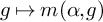 satisfies (Cotlar𝔼
⊥) for every
$\alpha $
satisfies (Cotlar𝔼
⊥) for every
$\alpha $
 , then

is clearly bounded in
$L_p(\mathcal {L} \mathrm {G})$
 for every
$1 < p < \infty $
for every
$1 < p < \infty $
 . We could add more flexibility to this technique by allowing the map
$g \mapsto m(\alpha , g)$
. We could add more flexibility to this technique by allowing the map
$g \mapsto m(\alpha , g)$
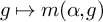 to be the product of k terms satisfying (Cotlar𝔼
⊥). Let us call this class
$\mathrm {coCot}^k(\mathrm {G})$
to be the product of k terms satisfying (Cotlar𝔼
⊥). Let us call this class
$\mathrm {coCot}^k(\mathrm {G})$
 . We leave mostly unexplored the following natural problem:
Problem 2.9. Let
$\mathrm {G}_0 \subseteq \mathrm {G}$
 and
$m:\mathrm {G} \to \mathbb {C}$
and
$m:\mathrm {G} \to \mathbb {C}$
 be as above. Are there sufficient conditions, for example in terms of smoothness, implying that
$m \in \mathrm {coCot}^k(\mathrm {G})$
be as above. Are there sufficient conditions, for example in terms of smoothness, implying that
$m \in \mathrm {coCot}^k(\mathrm {G})$
 ?
?
This remains as an underexplored approach to prove the boundedness of Fourier multipliers over groups without recourse to noncommutative analogues of singular integral theory. In fact, observe that in the classical case of
$\mathbb {R}$
 any function of bounded variation lies in the convex hull of (translations of) the classical Hilbert transform and therefore
$m \in \mathrm {BV}(\mathbb {R}) \implies m \in \mathrm {coCot}^1(\mathbb {R})$
any function of bounded variation lies in the convex hull of (translations of) the classical Hilbert transform and therefore
$m \in \mathrm {BV}(\mathbb {R}) \implies m \in \mathrm {coCot}^1(\mathbb {R})$
 , see [Reference Duoandikoetxea25, Corollary 3.8]. In higher dimensions the behaviour is even richer. For instance, let
$m:\mathbb {R}^2 \to \mathbb {C}$
, see [Reference Duoandikoetxea25, Corollary 3.8]. In higher dimensions the behaviour is even richer. For instance, let
$m:\mathbb {R}^2 \to \mathbb {C}$
 be a homogeneous function, i.e., a function satisfying that
$m(\lambda \, \xi ) = m(\xi )$
be a homogeneous function, i.e., a function satisfying that
$m(\lambda \, \xi ) = m(\xi )$
 for every
$\lambda> 0$
for every
$\lambda> 0$
 . Clearly, m depends only on its angular component
$m{|}_{\mathbb {T}}$
. Clearly, m depends only on its angular component
$m{|}_{\mathbb {T}}$
 . We have that

where
$\mathrm {BV}(\mathbb {T})$
 is the space of functions of bounded variation on the torus. To see that, just notice that the indicator function
${\mathbf {1}}_{\Sigma _\theta }$
is the space of functions of bounded variation on the torus. To see that, just notice that the indicator function
${\mathbf {1}}_{\Sigma _\theta }$
 of the sector
$\Sigma _\theta \subseteq \mathbb {R}^2$
of the sector
$\Sigma _\theta \subseteq \mathbb {R}^2$
 of all vectors whose polar angle
$\omega $
of all vectors whose polar angle
$\omega $
 lies in
$[0,\theta )$
lies in
$[0,\theta )$
 can be expressed as the product of the characteristic functions of two half-planes, each of which satisfies a Cotlar identity. Homogeneous functions of angular bounded variation can be expressed as convex combinations of different sector indicators.
Generalizations. It worth noticing that the identity (Cotlar𝔼 ⊥) can be generalized in a natural way by changing the equality by an operator inequality

for every
$f \in \mathcal {M} \cap L_2(\mathcal {M})$
 and some constant
$\Lambda \geq 0$
and some constant
$\Lambda \geq 0$
 . It is clear that this inequality implies the same bound (2.6) of Proposition 2.3 for left
$\mathcal {N}$
. It is clear that this inequality implies the same bound (2.6) of Proposition 2.3 for left
$\mathcal {N}$
 -modular operators, just with a constant growing like
$\mathrm {O}(1 + \sqrt {\Lambda })$
-modular operators, just with a constant growing like
$\mathrm {O}(1 + \sqrt {\Lambda })$
 . Similarly, there exists a closed-formula characterization of Fourier multipliers
$T_m$
. Similarly, there exists a closed-formula characterization of Fourier multipliers
$T_m$
 with left
$\mathrm {G}_0$
with left
$\mathrm {G}_0$
 -invariant symbol m satisfying (Cotlar𝔼
⊥≤). To formulate such characterization let us define
-invariant symbol m satisfying (Cotlar𝔼
⊥≤). To formulate such characterization let us define

and notice that (Cotlar𝔼 ⊥≤) is actually equivalent to

The inequality above is equivalent to the (integral) positivity of the operator-valued kernel
$\Omega _m(g,h) \, \lambda _{gh^{-1}}$
 . Since multiplication by
$\lambda _{g^{-1}} \cdot \lambda _h$
. Since multiplication by
$\lambda _{g^{-1}} \cdot \lambda _h$
 preserves positivity, this is equivalent to requiring that
$\Omega _m$
preserves positivity, this is equivalent to requiring that
$\Omega _m$
 be an integrally positive kernel, i.e.,

When
$\mathrm {G}$
 is discrete, this condition implies that
$\Omega _m$
is discrete, this condition implies that
$\Omega _m$
 factors as

where
$\xi : \mathrm {G} \to \mathcal {H}$
 is a bounded function with values in a Hilbert space
$\mathcal {H}$
is a bounded function with values in a Hilbert space
$\mathcal {H}$
 , see [Reference Bekka, de la Harpe and Valette3, Theorem C.1.4]. The reason why we need to add the term
$\Lambda \, \mathbb {E}[f \, f^\ast ]$
, see [Reference Bekka, de la Harpe and Valette3, Theorem C.1.4]. The reason why we need to add the term
$\Lambda \, \mathbb {E}[f \, f^\ast ]$
 to the Cotlar identity when
$\mathrm {G}_0$
to the Cotlar identity when
$\mathrm {G}_0$
 is open is that, without it, we will be forcing the kernel
$\Omega _m(g,h)$
is open is that, without it, we will be forcing the kernel
$\Omega _m(g,h)$
 to be positive definite while also vanishing on the diagonal
$g = h$
to be positive definite while also vanishing on the diagonal
$g = h$
 , which would imply that it is identically zero. In the non-relative case, this extra term can be omitted. This more general Cotlar identity leads to the following problem, which we leave unexplored.
Problem 2.10. Let
$\mathrm {G}_0 \subseteq \mathrm {G}$
 and
$m: \mathrm {G} \to \mathbb {C}$
and
$m: \mathrm {G} \to \mathbb {C}$
 be as above. Is there a geometric model of
$\mathrm {G} \curvearrowright \mathcal {X}$
be as above. Is there a geometric model of
$\mathrm {G} \curvearrowright \mathcal {X}$
 , possibly generalizing that of actions on UAC spaces in Theorem B, such that if
$m(g)$
, possibly generalizing that of actions on UAC spaces in Theorem B, such that if
$m(g)$
 lifts to
$\mathcal {X}$
lifts to
$\mathcal {X}$
 via a function
$m(g) = \widetilde {m}(g \cdot x_0)$
via a function
$m(g) = \widetilde {m}(g \cdot x_0)$
 , then its associated Fourier multiplier satisfies (Cotlar𝔼
⊥≤)?
, then its associated Fourier multiplier satisfies (Cotlar𝔼
⊥≤)?
3 Groups acting on
$\mathbb {R}$
-trees

Let X be a Hausdorff topological space. An arc
$\gamma $
 on X is a subset of X that is the image of an injective continuous function mapping
$[0, 1]$
on X is a subset of X that is the image of an injective continuous function mapping
$[0, 1]$
 onto
$\gamma $
onto
$\gamma $
 . The space X is said to be uniquely arcwise connected, or UAC, if any two points in X are joined by a unique arc. We say that a group
$\mathrm {G}$
. The space X is said to be uniquely arcwise connected, or UAC, if any two points in X are joined by a unique arc. We say that a group
$\mathrm {G}$
 acts on a UAC space X if
$\mathrm {G}$
acts on a UAC space X if
$\mathrm {G}$
 acts by homeomorphisms on X.
If, in addition, the UAC space X is metrisable and there is a metric
$d: X \times X \to \mathbb {C}$
 such that the unique arc joining two points is isometric to a closed interval of the real line, then
$(X, d)$
such that the unique arc joining two points is isometric to a closed interval of the real line, then
$(X, d)$
 is called an
$\mathbb {R}$
is called an
$\mathbb {R}$
 -tree. We will say that a group
$\mathrm {G}$
-tree. We will say that a group
$\mathrm {G}$
 acts on an
$\mathbb {R}$
acts on an
$\mathbb {R}$
 -tree X if it acts on it by isometries.
Observe that this definition is topological in nature since the underlying space is required to be arcwise connected. An alternative route to
$\mathbb {R}$
 -trees can be taken by defining them as hyperbolic spaces with
$\delta = 0$
-trees can be taken by defining them as hyperbolic spaces with
$\delta = 0$
 , i.e., every triangle is a tripod. These two definitions, although equivalent in spirit, are slightly different. Namely, a tree seen as a discrete set with the edge metric is a
$0$
, i.e., every triangle is a tripod. These two definitions, although equivalent in spirit, are slightly different. Namely, a tree seen as a discrete set with the edge metric is a
$0$
 -hyperbolic metric space but not an
$\mathbb {R}$
-hyperbolic metric space but not an
$\mathbb {R}$
 -tree in our definition. This is not a problem since trees can still be seen as a subclass of
$\mathbb {R}$
-tree in our definition. This is not a problem since trees can still be seen as a subclass of
$\mathbb {R}$
 -trees by treating them as simplicial trees, i.e. the one-dimensional simplicial complexes obtained from the incidence information of the tree. We also have that, given an
$\mathbb {R}$
-trees by treating them as simplicial trees, i.e. the one-dimensional simplicial complexes obtained from the incidence information of the tree. We also have that, given an
$\mathbb {R}$
 -tree X, if the set of points whose complement has three or more connected components is discrete in X, then X is a simplicial tree. The first definition of
$\mathbb {R}$
-tree X, if the set of points whose complement has three or more connected components is discrete in X, then X is a simplicial tree. The first definition of
$\mathbb {R}$
 -trees was given by Tits [Reference Tits, Bass, P.J. and J.85], then Morgan and Shalen [Reference Morgan and Shalen58], following earlier results of Alperin and Moss [Reference Alperin and Moss1], drew attention to the theory of
$\mathbb {R}$
-trees was given by Tits [Reference Tits, Bass, P.J. and J.85], then Morgan and Shalen [Reference Morgan and Shalen58], following earlier results of Alperin and Moss [Reference Alperin and Moss1], drew attention to the theory of
$\mathbb {R}$
 -trees by showing how to compactify a generalization of Teichmuller space for a finitely generated group using
$\mathbb {R}$
-trees by showing how to compactify a generalization of Teichmuller space for a finitely generated group using
$\mathbb {R}$
 -trees. We refer the reader to [Reference Bestvina, Daverman and Sher5] for more on
$\mathbb {R}$
-trees. We refer the reader to [Reference Bestvina, Daverman and Sher5] for more on
$\mathbb {R}$
 -trees.
We define the following two models for a group acting on a UAC space. Let
$\mathrm {G} \curvearrowright X$
 be a topological action and
$x_0 \in X$
be a topological action and
$x_0 \in X$
 a selected point. We will say that a bounded measurable function
$\varphi : X\setminus \{x_0\} \to \mathbb {C}$
a selected point. We will say that a bounded measurable function
$\varphi : X\setminus \{x_0\} \to \mathbb {C}$
 is constant along arcs iff
$\varphi (x) = \varphi (y)$
is constant along arcs iff
$\varphi (x) = \varphi (y)$
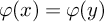 if there is an arc connecting x and y inside
$X \setminus \{x_0\}$
if there is an arc connecting x and y inside
$X \setminus \{x_0\}$
 . This is equivalent to decomposing
$X \setminus \{x_0\}$
. This is equivalent to decomposing
$X \setminus \{x_0\}$
 as a union of arcwise connected subsets and imposing the function to be constant over those subsets.
Model 1. Let
$\mathrm {G} \curvearrowright X$
 be a topological action on a UAC space,
$x_0 \in X$
be a topological action on a UAC space,
$x_0 \in X$
 a point and
$\widetilde {m}: X \to \mathbb {C}$
a point and
$\widetilde {m}: X \to \mathbb {C}$
 a bounded measurable function such that
-
(i) $\widetilde {m}$
, restricted to
$X \setminus \{x_0\}$
, is constant along arcs. -
(ii) $\widetilde {m}$
is invariant under the action
$\mathrm {St}_{x_0} \curvearrowright X \setminus \{x_0\}$
.



Then we define the multiplier
$m: \mathrm {G} \to \mathbb {C}$
 as
as

and fix
$(\mathrm {G}_0, \mathrm {G})$
 as
$(\mathrm {St}_{x_0}, \mathrm {G})$
as
$(\mathrm {St}_{x_0}, \mathrm {G})$
 .
.
This definition has the drawback that the invariance under
$\mathrm {St}_{x_0}$
 of m can make the symbol constant outside
$\mathrm {St}_{x_0}$
of m can make the symbol constant outside
$\mathrm {St}_{x_0}$
 in some cases. We introduce the following, more involved, model.
Model 2. Let us fix two distinct constants
$C_1$
 ,
$C_2 \in \mathbb {C}$
,
$C_2 \in \mathbb {C}$
 . Let similarly
$\mathrm {G} \curvearrowright X$
. Let similarly
$\mathrm {G} \curvearrowright X$
 be a topological action on a UAC space and
$x_0 \in X$
be a topological action on a UAC space and
$x_0 \in X$
 a point. Choose
$X_0 \subseteq X \setminus \{x_0\}$
a point. Choose
$X_0 \subseteq X \setminus \{x_0\}$
 to be an arcwise connected subset. We define
$m: \mathrm {G} \to \mathbb {C}$
to be an arcwise connected subset. We define
$m: \mathrm {G} \to \mathbb {C}$
 to be
to be

We will also fix
$\mathrm {G}_0$
 to be
$\mathrm {St}_{x_0} \cap \{ g \in \mathrm {G} : g \cdot X_0 = X_0 \}$
to be
$\mathrm {St}_{x_0} \cap \{ g \in \mathrm {G} : g \cdot X_0 = X_0 \}$
 .
.
Observe that Model 2 is a natural modification of Model 1 for the function
$\widetilde {m}: X \to \mathbb {C}$
 given by
$\widetilde {m} = C_1 {\mathbf {1}}_{X\setminus (\{ x_0\}\cup X_0)} + C_2 {\mathbf {1}}_{X_0}$
given by
$\widetilde {m} = C_1 {\mathbf {1}}_{X\setminus (\{ x_0\}\cup X_0)} + C_2 {\mathbf {1}}_{X_0}$
 . The main difference is that we extend the value of
$C_1$
. The main difference is that we extend the value of
$C_1$
 to a portion of the stabilizer.
Proposition 3.1. Let
$\mathrm {G} \curvearrowright X$
 be an action as above.
-
(i) Let $m: \mathrm {G} \to \mathbb {C}$
and
$\mathrm {G}_0$
be like in Model 1. Then,
$T_m$
satisfies (Cotlar𝔼
⊥) relative to
$\mathrm {G}_0$
and is left
$\mathcal {L} \mathrm {G}_0$
-modular. -
(ii) Let $m: \mathrm {G} \to \mathbb {C}$
and
$\mathrm {G}_0$
be like in Model 2. Then,
$T_m$
satisfies (Cotlar𝔼
⊥) relative to
$\mathrm {G}_0$
and is left
$\mathcal {L} \mathrm {G}_0$
-modular.


The points above imply that
$T_m$
 in both Models 1 and 2 are bounded in
$L_p(\mathcal {L} \mathrm {G})$
in both Models 1 and 2 are bounded in
$L_p(\mathcal {L} \mathrm {G})$
 for
$1 < p < \infty $
for
$1 < p < \infty $
 .
.
Proof. The statement in point (i) has already been proved in the introduction. Thus, we concentrate on point (ii). The fact that m is left invariant under the action of
$\mathrm {G}_0 = \{ g \in \mathrm {G} : g \cdot x_0 = x_0 \} \cap \{ g \in \mathrm {G} : g \cdot X_0 = X_0 \}$
 is immediate. Now, all we have to do is to verify (Cotla ^r). To that end, let us divide the group as a disjoint union
$\mathrm {G} = \mathrm {G}_0 \cup \mathrm {G}_1 \cup \mathrm {G}_2 \cup \mathrm {G}_3$
is immediate. Now, all we have to do is to verify (Cotla ^r). To that end, let us divide the group as a disjoint union
$\mathrm {G} = \mathrm {G}_0 \cup \mathrm {G}_1 \cup \mathrm {G}_2 \cup \mathrm {G}_3$
 , where

Observe also that, since m is both left and right
$\mathrm {G}_0$
 -invariant, it is enough to verify (Cotla ^r) for
$g, h \in \mathrm {G} \setminus \mathrm {G}_0$
-invariant, it is enough to verify (Cotla ^r) for
$g, h \in \mathrm {G} \setminus \mathrm {G}_0$
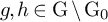 . Assume that
$m(g^{-1}) \neq m(h)$
. Assume that
$m(g^{-1}) \neq m(h)$
 , otherwise we are done, our aim is to show that
$m(g h) = m(g)$
, otherwise we are done, our aim is to show that
$m(g h) = m(g)$
 . We will proceed by cases. First, assume that
$g \in \mathrm {G}_1$
. We will proceed by cases. First, assume that
$g \in \mathrm {G}_1$
 . This is equivalent to
$g^{-1} \in \mathrm {G}_1$
. This is equivalent to
$g^{-1} \in \mathrm {G}_1$
 and therefore
$h \in \mathrm {G}_3$
and therefore
$h \in \mathrm {G}_3$
 . But then,
$g \, h \cdot x_0 \not \in X_0$
. But then,
$g \, h \cdot x_0 \not \in X_0$
 and
$g \, h \cdot x_0 \neq x_0$
and
$g \, h \cdot x_0 \neq x_0$
 . Therefore
$g \, h \in \mathrm {G}_2$
. Therefore
$g \, h \in \mathrm {G}_2$
 and we get
$m(g h) = m(g)$
and we get
$m(g h) = m(g)$
 . In the case of
$g \in \mathrm {G}_2$
. In the case of
$g \in \mathrm {G}_2$
 we have the whole range of possibilities and h can belong to
$\mathrm {G}_1$
we have the whole range of possibilities and h can belong to
$\mathrm {G}_1$
 ,
$\mathrm {G}_2$
,
$\mathrm {G}_2$
 or
$\mathrm {G}_3$
or
$\mathrm {G}_3$
 . In the case of
$g \in \mathrm {G}_2$
. In the case of
$g \in \mathrm {G}_2$
 and
$h \in \mathrm {G}_1$
and
$h \in \mathrm {G}_1$
 we have that
$g h \in \mathrm {G}_2$
we have that
$g h \in \mathrm {G}_2$
 . Indeed,
$g h \cdot x_0 = g \cdot x_0 \not \in X_0$
. Indeed,
$g h \cdot x_0 = g \cdot x_0 \not \in X_0$
 and it is immediate that
$g h$
and it is immediate that
$g h$
 is not in the stabilizer of
$x_0$
is not in the stabilizer of
$x_0$
 . For the second case of
$g \in \mathrm {G}_2$
. For the second case of
$g \in \mathrm {G}_2$
 and
$h \in \mathrm {G}_2$
and
$h \in \mathrm {G}_2$
 the condition
$m(g^{-1}) \neq m(h)$
the condition
$m(g^{-1}) \neq m(h)$
 implies that
$g^{-1} \cdot x_0$
implies that
$g^{-1} \cdot x_0$
 and
$h \cdot x_0$
and
$h \cdot x_0$
 live in distinct arcwise connected subsets of
$X \setminus \{x_0\}$
live in distinct arcwise connected subsets of
$X \setminus \{x_0\}$
 . But then there is a unique path connecting both points that passes through the root. Applying g to the whole arc gives that
$g \cdot x_0$
. But then there is a unique path connecting both points that passes through the root. Applying g to the whole arc gives that
$g \cdot x_0$
 and
$g h \cdot x_0$
and
$g h \cdot x_0$
 lie in the same arcwise connected subset and do not stabilize
$x_0$
lie in the same arcwise connected subset and do not stabilize
$x_0$
 , see Figure 1. Therefore
$m(g h) = m(g)$
, see Figure 1. Therefore
$m(g h) = m(g)$
 . The third case is given by
$g \in \mathrm {G}_2$
. The third case is given by
$g \in \mathrm {G}_2$
 and
$h \in \mathrm {G}_3$
and
$h \in \mathrm {G}_3$
 . Observe that if
$g \in \mathrm {G}_2$
. Observe that if
$g \in \mathrm {G}_2$
 , then
$g^{-1}$
, then
$g^{-1}$
 can only be inside
$\mathrm {G}_2$
can only be inside
$\mathrm {G}_2$
 or
$\mathrm {G}_3$
or
$\mathrm {G}_3$
 . But the case
$g^{-1} \in \mathrm {G}_3$
. But the case
$g^{-1} \in \mathrm {G}_3$
 can be easily discarded since it will contradict the assumption
$m(g^{-1}) \neq m(h)$
can be easily discarded since it will contradict the assumption
$m(g^{-1}) \neq m(h)$
 . But if
$g^{-1} \in \mathrm {G}_2$
. But if
$g^{-1} \in \mathrm {G}_2$
 and
$h \in \mathrm {G}_3$
and
$h \in \mathrm {G}_3$
 , then
$g^{-1} \cdot x_0$
, then
$g^{-1} \cdot x_0$
 and
$h \cdot x_0$
and
$h \cdot x_0$
 live in distinct arcwise connected subsets and we can proceed like in the previous case. It remains to check the case of
$g \in \mathrm {G}_3$
live in distinct arcwise connected subsets and we can proceed like in the previous case. It remains to check the case of
$g \in \mathrm {G}_3$
 . We have that h can be in either
$\mathrm {G}_1$
. We have that h can be in either
$\mathrm {G}_1$
 ,
$\mathrm {G}_2$
,
$\mathrm {G}_2$
 or
$\mathrm {G}_3$
or
$\mathrm {G}_3$
 . In the first case we deduce that
$g h \in \mathrm {G}_3$
. In the first case we deduce that
$g h \in \mathrm {G}_3$
 . For the second one we have that if
$g \in \mathrm {G}_3$
. For the second one we have that if
$g \in \mathrm {G}_3$
 and
$h \in \mathrm {G}_2$
and
$h \in \mathrm {G}_2$
 , then we can assume that
$g^{-1} \in \mathrm {G}_3$
, then we can assume that
$g^{-1} \in \mathrm {G}_3$
 , the only other choice being
$g^{-1} \in \mathrm {G}_2$
, the only other choice being
$g^{-1} \in \mathrm {G}_2$
 which will contradict the assumption
$m(g^{-1}) \neq m(h)$
which will contradict the assumption
$m(g^{-1}) \neq m(h)$
 . But this implies that
$g^{-1} \cdot x_0$
. But this implies that
$g^{-1} \cdot x_0$
 and
$h \cdot x_0$
and
$h \cdot x_0$
 live in different arcwise connected subsets of
$X \setminus \{x_0\}$
live in different arcwise connected subsets of
$X \setminus \{x_0\}$
 and we can apply the argument in Figure 1. Lastly, if
$g \in \mathrm {G}_3$
and we can apply the argument in Figure 1. Lastly, if
$g \in \mathrm {G}_3$
 and
$h \in \mathrm {G}_3$
and
$h \in \mathrm {G}_3$
 we obtain similarly that
$g^{-1}$
we obtain similarly that
$g^{-1}$
 can only lie in
$\mathrm {G}_2$
can only lie in
$\mathrm {G}_2$
 . The same path argument applies. Applying Theorem B, we get the
$L_p$
. The same path argument applies. Applying Theorem B, we get the
$L_p$
 -boundedness of
$T_m$
-boundedness of
$T_m$
 .
.
Remark 3.2. Recall also that, by Remark 2.5, when the subgroup
$\mathrm {St}_{x_0}$
 has empty interior, condition (2) in Model 1 can be dropped.
Observe that in the case of
$\mathrm {G} = \mathbb {R}$
 , the Hilbert transform is also of weak type
$(1,1)$
, the Hilbert transform is also of weak type
$(1,1)$
 , i.e.,
$H:L_1(\mathbb {R}) \to L_{1,\infty }(\mathbb {R})$
, i.e.,
$H:L_1(\mathbb {R}) \to L_{1,\infty }(\mathbb {R})$
 and bounded between
$L_\infty (\mathbb {R})$
and bounded between
$L_\infty (\mathbb {R})$
 and the space of bounded mean oscillation functions
$\mathrm {BMO}(\mathbb {R})$
and the space of bounded mean oscillation functions
$\mathrm {BMO}(\mathbb {R})$
 . Both endpoint spaces give – by either complex or real interpolation with
$L_2$
. Both endpoint spaces give – by either complex or real interpolation with
$L_2$
 – the optimal order for the operator
$L_p$
– the optimal order for the operator
$L_p$
 norm of H. The following problem remains open.
Problem 3.3. Let
$\mathrm {G}$
 be a group and m a multiplier like in Model 1 or 2. Is it possible to construct spaces
$\mathrm {X}_1$
be a group and m a multiplier like in Model 1 or 2. Is it possible to construct spaces
$\mathrm {X}_1$
 and
$\mathrm {X}_\infty $
and
$\mathrm {X}_\infty $
 , in place of
$L_{1,\infty }$
, in place of
$L_{1,\infty }$
 and
$\mathrm {BMO}$
and
$\mathrm {BMO}$
 , such that
-
(i) $\| T_m: L_1(\mathcal {L} \mathrm {G}) \to \mathrm {X}_1 \| < \infty $
and
$\| T_m: L_\infty (\mathcal {L} \mathrm {G}) \to \mathrm {X}_\infty \| < \infty $
, -
(ii) interpolation of $\mathrm {X}_1$
or
$\mathrm {X}_\infty $
with
$L_2$
yields growth of
$\max \{p, p'\}$
for the operator
$L_p$
norm of
$T_m$
?




This problem presents at least three challenges. The first difficulty comes from the fact that weak type
$(1,1)$
 bounds are difficult to obtain for noncommutative singular integral type operators. They are known in some semicommutative examples [Reference Parcet62, Reference Cadilhac, Conde-Alonso and Parcet8] but open in the case of Quantum Euclidean spaces [Reference González-Pérez, Junge and Parcet33] and in most group settings besides left-orderable groups [Reference Randrianantoanina74]. The second challenge is that the specific endpoint space
$\mathrm {X}_\infty $
bounds are difficult to obtain for noncommutative singular integral type operators. They are known in some semicommutative examples [Reference Parcet62, Reference Cadilhac, Conde-Alonso and Parcet8] but open in the case of Quantum Euclidean spaces [Reference González-Pérez, Junge and Parcet33] and in most group settings besides left-orderable groups [Reference Randrianantoanina74]. The second challenge is that the specific endpoint space
$\mathrm {X}_\infty $
 to be used for m in Model 1 or Model 2 has to be defined in terms of the geometry of
$\mathrm {G} \curvearrowright X$
to be used for m in Model 1 or Model 2 has to be defined in terms of the geometry of
$\mathrm {G} \curvearrowright X$
 and it cannot just be the usual noncommutative
$\mathrm {BMO}$
and it cannot just be the usual noncommutative
$\mathrm {BMO}$
 space, see [Reference Junge and Mei43, Reference Mei53, Reference Mei54]. Indeed, there is a natural unital and completely positive semigroup
$S_t: \mathcal {L} \mathbb {F}_2 \to \mathcal {L} \mathbb {F}_2$
space, see [Reference Junge and Mei43, Reference Mei53, Reference Mei54]. Indeed, there is a natural unital and completely positive semigroup
$S_t: \mathcal {L} \mathbb {F}_2 \to \mathcal {L} \mathbb {F}_2$
 in the free group algebra given by
$S_t(\lambda _g) = e^{-t|g|}$
in the free group algebra given by
$S_t(\lambda _g) = e^{-t|g|}$
 , see [Reference Haagerup36]. This semigroup allows to construct a natural and interpolating semigroup
$\mathrm {BMO}$
, see [Reference Haagerup36]. This semigroup allows to construct a natural and interpolating semigroup
$\mathrm {BMO}$
 space
$\mathrm {BMO}(\mathcal {L} \mathbb {F}_2)$
space
$\mathrm {BMO}(\mathcal {L} \mathbb {F}_2)$
 , see [Reference Junge, Mei and Parcet44]. But it is known that the multipliers (MR) are unbounded from
$L_\infty (\mathcal {L} \mathbb {F}_2)$
, see [Reference Junge, Mei and Parcet44]. But it is known that the multipliers (MR) are unbounded from
$L_\infty (\mathcal {L} \mathbb {F}_2)$
 to
$\mathrm {BMO}(\mathcal {L} \mathbb {F}_2)$
to
$\mathrm {BMO}(\mathcal {L} \mathbb {F}_2)$
 , see [Reference Mei, Ricard and Xu56, Appendix A]. The third difficulty comes from the fact that the classical technique, employed by Kolmogorov [Reference Kolmogorov50], of comparing a singular integral operator with a maximal one is delicate in this context since some of the operators obtained are not positivity preserving, which makes interpolating maximal functions an open problem [Reference Junge and Xu47]. The technique of Kolmogorov has been used in the noncommutative case in [Reference Hong, Lai and Xu40]. We will also mention that some tentative progress in the direction of Problem 3.3 has been made. For instance, Gała̧zka and Osękowski [Reference Gała̧zka and Osȩkowski30] have lowered the operator
$L_p$
, see [Reference Mei, Ricard and Xu56, Appendix A]. The third difficulty comes from the fact that the classical technique, employed by Kolmogorov [Reference Kolmogorov50], of comparing a singular integral operator with a maximal one is delicate in this context since some of the operators obtained are not positivity preserving, which makes interpolating maximal functions an open problem [Reference Junge and Xu47]. The technique of Kolmogorov has been used in the noncommutative case in [Reference Hong, Lai and Xu40]. We will also mention that some tentative progress in the direction of Problem 3.3 has been made. For instance, Gała̧zka and Osękowski [Reference Gała̧zka and Osȩkowski30] have lowered the operator
$L_p$
 -norm of the Fourier multiplier
$m: \mathbb {F}_2 \to \mathbb {C}$
-norm of the Fourier multiplier
$m: \mathbb {F}_2 \to \mathbb {C}$
 that depends on the starting letter from
$\mathrm {O}(p^\beta )$
that depends on the starting letter from
$\mathrm {O}(p^\beta )$
 to
$\mathrm {O}(p \log p)$
to
$\mathrm {O}(p \log p)$
 as
$p \to \infty $
as
$p \to \infty $
 .
.
Now, we are going to study Models 1 and 2 in the context of
$\mathbb {R}$
 -trees. Observe that, since any
$\mathbb {R}$
-trees. Observe that, since any
$\mathbb {R}$
 -tree action is an action of the underlying UAC topological space, Proposition 3.1 above works for
$\mathbb {R}$
-tree action is an action of the underlying UAC topological space, Proposition 3.1 above works for
$\mathbb {R}$
 -trees. Furthermore, in the case of group actions on
$\mathbb {R}$
-trees. Furthermore, in the case of group actions on
$\mathbb {R}$
 -trees we have the following result connecting the existence of global fixed points with the form of the Fourier multiplier
$T_m$
-trees we have the following result connecting the existence of global fixed points with the form of the Fourier multiplier
$T_m$
 . We are going to say that the multipliers m coming from Models 1 and 2 are trivial iff they are constant for any
$g \in \mathrm {G} \setminus \mathrm {G}_0$
. We are going to say that the multipliers m coming from Models 1 and 2 are trivial iff they are constant for any
$g \in \mathrm {G} \setminus \mathrm {G}_0$
 .
.
Proposition 3.4. Let X be an
$\mathbb {R}$
 -tree and
$\mathrm {G} \curvearrowright X$
-tree and
$\mathrm {G} \curvearrowright X$
 an (isometric) action of a discrete group. The following holds:
-
(i) If the action $\mathrm {G} \curvearrowright X$
has a global fixed point, then for any choice of a root
$x_0 \in X$
the multipliers in Model 1 and Model 2 are trivial. -
(ii) If $\mathrm {G}$
is finitely generated, for any action on an
$\mathbb {R}$
-tree X, there is either a global fixed point or there exists
$x_0 \in X$
such that the corresponding symbol given in Model 2 is nontrivial.


Proof. We will prove first (i) for m as in Model 1. Assume that the action has a global fixed point
$x_1 \in X$
 . If
$x_1$
. If
$x_1$
 coincides with the root
$x_0$
coincides with the root
$x_0$
 then
$m = 0$
then
$m = 0$
 and there is nothing to prove. Therefore we assume
$x_0 \neq x_1$
and there is nothing to prove. Therefore we assume
$x_0 \neq x_1$
 . Similarly, we can assume without loss of generality that
$\mathrm {St}_{x_0}\neq \mathrm {G}$
. Similarly, we can assume without loss of generality that
$\mathrm {St}_{x_0}\neq \mathrm {G}$
 , since otherwise
$m = 0$
, since otherwise
$m = 0$
 . Pick
$g \in \mathrm {G}$
. Pick
$g \in \mathrm {G}$
 and assume that
$g \cdot x_0$
and assume that
$g \cdot x_0$
 lies in an arcwise connected subset of
$X \setminus \{x_0\}$
lies in an arcwise connected subset of
$X \setminus \{x_0\}$
 different from that of
$x_1$
different from that of
$x_1$
 . Then, there is a unique path joining
$x_1$
. Then, there is a unique path joining
$x_1$
 and
$g \cdot x_0$
and
$g \cdot x_0$
 that passes through the root
$x_0$
that passes through the root
$x_0$
 , see Figure 2. But since
$x_1$
, see Figure 2. But since
$x_1$
 is fixed by any
$g\in \mathrm {G}$
is fixed by any
$g\in \mathrm {G}$
 , after applying g to the path we obtain a larger path, which contradicts the fact that the action is isometric.
The action of g over the path connecting the global fixed point and
$g \cdot x_0$
 .
.
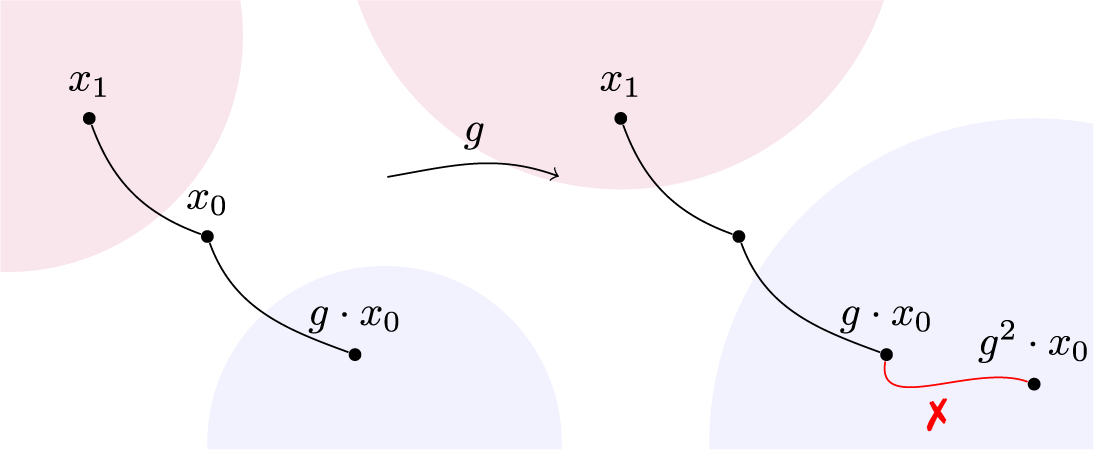
Figure 2 Long description
The diagram consists of two panels separated by a central arrow labeled g pointing from left to right.
In the left panel, a curved black line connects three points. The top point is x sub 1, located within a pink circular region. The middle point is x sub 0. The bottom point is g dot x sub 0, located within a light blue circular region.
In the right panel, the transformation is shown. The path starting from x sub 1 (now in a larger pink region) passes through x sub 0 and reaches g dot x sub 0 (now in a larger blue region). A new red segment continues from g dot x sub 0 to a final point labeled g squared dot x sub 0. A red X mark is placed below this final red segment.
This implies that
$g^2 \cdot x_0 = g \cdot x_0$
 and so
$g \cdot x_0 = x_0$
and so
$g \cdot x_0 = x_0$
 , which contradicts the assumptions. Therefore,
$g \cdot x_0$
, which contradicts the assumptions. Therefore,
$g \cdot x_0$
 belongs to the same connected subset of
$x_1$
belongs to the same connected subset of
$x_1$
 for every g that do not stabilize the root
$x_0$
for every g that do not stabilize the root
$x_0$
 , that is,
$m(g)$
, that is,
$m(g)$
 is constant for any
$g\in \mathrm {G}\setminus \mathrm {St}_{x_0}$
is constant for any
$g\in \mathrm {G}\setminus \mathrm {St}_{x_0}$
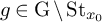 .
.
For the case of m as in Model 2, let
$x_1 \in X$
 be a global fixed point. We can again consider without loss of generality that
$x_0 \neq x_1$
be a global fixed point. We can again consider without loss of generality that
$x_0 \neq x_1$
 and that
$\mathrm {St}_{x_0}\neq \mathrm {G}$
and that
$\mathrm {St}_{x_0}\neq \mathrm {G}$
 . By those assumptions, there exists
$g_0 \in \mathrm {G}$
. By those assumptions, there exists
$g_0 \in \mathrm {G}$
 with
$g_0 \cdot x_0 \in X \setminus \{x_0\}$
with
$g_0 \cdot x_0 \in X \setminus \{x_0\}$
 . We have two possibilities for
$g_0$
. We have two possibilities for
$g_0$
 . If
$g_0 \cdot x_0 \neq x_0$
. If
$g_0 \cdot x_0 \neq x_0$
 and
$g_0 \cdot x_0 \not \in X_0$
and
$g_0 \cdot x_0 \not \in X_0$
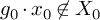 , then
$m(g_0) = C_1$
, then
$m(g_0) = C_1$
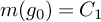 , while if
$g_0 \cdot x_0 \in X_0$
, while if
$g_0 \cdot x_0 \in X_0$
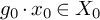 then
$m(g_0) = C_2$
then
$m(g_0) = C_2$
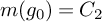 . If we are in the first case
$g_0 \cdot x_0 \not \in X_0$
. If we are in the first case
$g_0 \cdot x_0 \not \in X_0$
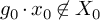 , then the multiplier m will be trivial unless there exists a
$g_1 \in \mathrm {G}$
, then the multiplier m will be trivial unless there exists a
$g_1 \in \mathrm {G}$
 such that
$g_1 \cdot x_0 \in X_0$
such that
$g_1 \cdot x_0 \in X_0$
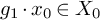 . Let us obtain a contradiction. First, we claim that the global fixed point
$x_1 \not \in X_0$
. Let us obtain a contradiction. First, we claim that the global fixed point
$x_1 \not \in X_0$
 . Assume
$x_1 \in X_0$
. Assume
$x_1 \in X_0$
 . Then, there is a path joining
$x_1$
. Then, there is a path joining
$x_1$
 and
$g_0 \cdot x_0$
and
$g_0 \cdot x_0$
 that passes through the root
$x_0$
that passes through the root
$x_0$
 , see Figure 3. But applying
$g_0$
, see Figure 3. But applying
$g_0$
 to the path gives that
$g_0 \cdot x_0 = x_0$
to the path gives that
$g_0 \cdot x_0 = x_0$
 which is a contradiction. Therefore
$x_1 \not \in X_0$
which is a contradiction. Therefore
$x_1 \not \in X_0$
 , but since
$g_1 \cdot x_0 \in X_0$
, but since
$g_1 \cdot x_0 \in X_0$
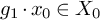 , we can build a path from
$x_1$
, we can build a path from
$x_1$
 to
$g_1 \cdot x_0$
to
$g_1 \cdot x_0$
 that passes through the root
$x_0$
that passes through the root
$x_0$
 and, repeating the same argument as before, obtain that
$g_1 \cdot x_0 = x_0$
and, repeating the same argument as before, obtain that
$g_1 \cdot x_0 = x_0$
 , which is a contradiction. For the second case
$g_0 \cdot x_0 \in X_0$
, which is a contradiction. For the second case
$g_0 \cdot x_0 \in X_0$
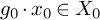 . First, we notice that
$x_1$
. First, we notice that
$x_1$
 must live in
$X_0$
must live in
$X_0$
 , if not, proceeding as before we will get that
$g_0 \cdot x_0 = x_0$
, if not, proceeding as before we will get that
$g_0 \cdot x_0 = x_0$
 , which is a contradiction. In order for m to be nontrivial there should be a
$g_1 \in \mathrm {G}$
, which is a contradiction. In order for m to be nontrivial there should be a
$g_1 \in \mathrm {G}$
 such that either
$g_1 \cdot x_0 = x_0$
such that either
$g_1 \cdot x_0 = x_0$
 and
$g_1 \cdot X_0 \neq X_0$
and
$g_1 \cdot X_0 \neq X_0$
 or
$g_1 \cdot x_0 \neq x_0$
or
$g_1 \cdot x_0 \neq x_0$
 and
$g_1 \cdot x_0 \not \in X_0$
and
$g_1 \cdot x_0 \not \in X_0$
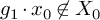 . For the first case, let us choose a point
$x_2 \in X_0$
. For the first case, let us choose a point
$x_2 \in X_0$
 . Then,
$g_1 \cdot x_2 \not \in X_0$
. Then,
$g_1 \cdot x_2 \not \in X_0$
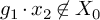 and similarly
$g_1 \cdot x_2 \neq x_0$
and similarly
$g_1 \cdot x_2 \neq x_0$
 . Now, construct a path joining
$x_1$
. Now, construct a path joining
$x_1$
 with
$g_1 \cdot x_2$
with
$g_1 \cdot x_2$
 . Since
$x_1 \in X_0$
. Since
$x_1 \in X_0$
 but
$g_1 \cdot x_2$
but
$g_1 \cdot x_2$
 belongs to a different connected subset, the arc joining them passes through the root
$x_0$
belongs to a different connected subset, the arc joining them passes through the root
$x_0$
 . Let us apply
$g_1^{-1}$
. Let us apply
$g_1^{-1}$
 to the whole arc. Since we have that
$g_1^{-1} \cdot x_0 = x_0$
to the whole arc. Since we have that
$g_1^{-1} \cdot x_0 = x_0$
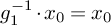 , we obtain an arc that joins
$x_1$
, we obtain an arc that joins
$x_1$
 and
$x_2$
and
$x_2$
 and passes through the root
$x_0$
and passes through the root
$x_0$
 . But this is a contradiction with the fact that
$x_1$
. But this is a contradiction with the fact that
$x_1$
 and
$x_2$
and
$x_2$
 both belong to
$X_0$
both belong to
$X_0$
 , see Figure 4, since X is a UAC space the arc joining two elements in the same connected subset of
$X \setminus \{x_0\}$
, see Figure 4, since X is a UAC space the arc joining two elements in the same connected subset of
$X \setminus \{x_0\}$
 cannot pass trough the root
$x_0$
cannot pass trough the root
$x_0$
 . The remaining case is when
$g_1 \cdot x_0 \neq x_0$
. The remaining case is when
$g_1 \cdot x_0 \neq x_0$
 and
$g_1 \cdot x_0 \not \in X_0$
and
$g_1 \cdot x_0 \not \in X_0$
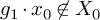 . Then, the arc joining
$x_1 \in X_0$
. Then, the arc joining
$x_1 \in X_0$
 and
$g_1 \cdot x_1$
and
$g_1 \cdot x_1$
 passes through
$x_0$
passes through
$x_0$
 . Applying
$g_1$
. Applying
$g_1$
 gives a contradiction with the fact that the action is isometric and that
$g_1 \cdot x_0 \neq x_0$
gives a contradiction with the fact that the action is isometric and that
$g_1 \cdot x_0 \neq x_0$
 . For the other point, if
$\mathrm {G}$
. For the other point, if
$\mathrm {G}$
 is finitely generated, the converse statement is also true and it is a corollary of [Reference Bowditch6, Lemma 5.2]. This lemma tells us that when a finitely generated group
$\mathrm {G}$
is finitely generated, the converse statement is also true and it is a corollary of [Reference Bowditch6, Lemma 5.2]. This lemma tells us that when a finitely generated group
$\mathrm {G}$
 acts non-trivially on an
$\mathbb {R}$
acts non-trivially on an
$\mathbb {R}$
 -tree X, there exist a point
$y_0$
-tree X, there exist a point
$y_0$
 and elements
$g, h \in \mathrm {G}$
and elements
$g, h \in \mathrm {G}$
 such that
$y_0$
such that
$y_0$
 lies in the arc between
$g \cdot y_0$
lies in the arc between
$g \cdot y_0$
 and
$h \cdot y_0$
and
$h \cdot y_0$
 and
$y_0$
and
$y_0$
 ,
$g \cdot y_0$
,
$g \cdot y_0$
 and
$h \cdot y_0$
and
$h \cdot y_0$
 are all different. Therefore, if
$\mathrm {G}$
are all different. Therefore, if
$\mathrm {G}$
 does not have property (F
$\mathbb {R}$
does not have property (F
$\mathbb {R}$
 ), we can choose
$x_0$
), we can choose
$x_0$
 as
$y_0$
as
$y_0$
 and
$X_0$
and
$X_0$
 as the maximally connected subset of
$g \cdot y_0$
as the maximally connected subset of
$g \cdot y_0$
 . Then, there is an
$h \in \mathrm {G}$
. Then, there is an
$h \in \mathrm {G}$
 such that
$h \cdot x_0 \neq x_0$
such that
$h \cdot x_0 \neq x_0$
 and
$h \cdot x_0 \not \in X_0$
and
$h \cdot x_0 \not \in X_0$
 . Thus, sending g and h to different values
$C_1$
. Thus, sending g and h to different values
$C_1$
 and
$C_2$
and
$C_2$
 gives a nontrivial multiplier within Model 2.
The action of
$g_0$
 over the path connecting
$x_1$
over the path connecting
$x_1$
 and
$g_0 \cdot x_0 \not \in X_0$
and
$g_0 \cdot x_0 \not \in X_0$
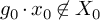 .
.

Figure 3 Long description
A mathematical diagram with two main sections separated by a curved arrow labeled g sub 0 pointing from left to right.
Left section: A curved black path connects three points. The top point x sub 1 is inside a pink circular region labeled X sub 0. The middle point is x sub 0. The bottom point is g sub 0 dot x sub 0, which sits inside a light blue circular region.
Right section: The same path from the left is repeated, starting at x sub 1 in a pink region X sub 0 and passing through x sub 0 and g sub 0 dot x sub 0. However, a new red segment extends from g sub 0 dot x sub 0 to a final point g sub 0 squared dot x sub 0. A large red X is placed below this final segment, indicating an invalid or restricted path extension.
The action of
$g_1^{-1}$
 over the path connecting
$x_1$
over the path connecting
$x_1$
 and
$g_1 \cdot x_2$
and
$g_1 \cdot x_2$
 .
.

Many groups we are familiar with admit actions on
$\mathbb {R}$
 -trees. For example, every finitely generated hyperbolic group. Indeed, a finitely generated group is hyperbolic if and only if every asymptotic cone of the group is an
$\mathbb {R}$
-trees. For example, every finitely generated hyperbolic group. Indeed, a finitely generated group is hyperbolic if and only if every asymptotic cone of the group is an
$\mathbb {R}$
 -tree [Reference Gromov35]. Then, the action of a hyperbolic group on its Cayley graph induces an action on the asymptotic cone of the Cayley graph. Moreover, any surface group having Euler characteristic less than
$-1$
-tree [Reference Gromov35]. Then, the action of a hyperbolic group on its Cayley graph induces an action on the asymptotic cone of the Cayley graph. Moreover, any surface group having Euler characteristic less than
$-1$
 acts freely on an
$\mathbb {R}$
acts freely on an
$\mathbb {R}$
 -tree [Reference Morgan and Shalen59].
On the other hand, there are many examples of groups for which any action on an
$\mathbb {R}$
 -tree has a global fixed point. When this happens the group
$\mathrm {G}$
-tree has a global fixed point. When this happens the group
$\mathrm {G}$
 is said to have property (F
$\mathbb {R}$
is said to have property (F
$\mathbb {R}$
 ), see [Reference Bestvina, Daverman and Sher5, Reference Shalen80]. The following corollary of Proposition 3.4 characterizes groups with property (F
$\mathbb {R}$
), see [Reference Bestvina, Daverman and Sher5, Reference Shalen80]. The following corollary of Proposition 3.4 characterizes groups with property (F
$\mathbb {R}$
 ).
).
Corollary 3.5.
$\mathrm {G}$
 has property (F
$\mathbb {R}$
has property (F
$\mathbb {R}$
 ) if and only if the symbol m in Model 2 is trivial for any
$x_0 \in X$
) if and only if the symbol m in Model 2 is trivial for any
$x_0 \in X$
 in any
$\mathbb {R}$
in any
$\mathbb {R}$
 -tree X on which
$\mathrm {G}$
-tree X on which
$\mathrm {G}$
 acts (isometrically).
One natural question, that we leave open, is whether there are functions
$m: \mathrm {G} \to \mathbb {C}$
 satisfying (Cotlar) for
$\mathrm {G}_0 = \{e\}$
satisfying (Cotlar) for
$\mathrm {G}_0 = \{e\}$
 and such that they do not lift to a function
$\widetilde {m}$
and such that they do not lift to a function
$\widetilde {m}$
 on a UAC space like in Model 1 or 2 on which
$\mathrm {G}$
on a UAC space like in Model 1 or 2 on which
$\mathrm {G}$
 acts. One way to prove the non-existence of such lift
$\widetilde {m}$
acts. One way to prove the non-existence of such lift
$\widetilde {m}$
 would be a procedure to assemble from the group
$\mathrm {G}$
would be a procedure to assemble from the group
$\mathrm {G}$
 and the function m a
$\mathrm {G}$
and the function m a
$\mathrm {G}$
 -space X on which
$\mathrm {G}$
-space X on which
$\mathrm {G}$
 acts naturally and a lift
$\widetilde {m}: X \to \mathbb {C}$
acts naturally and a lift
$\widetilde {m}: X \to \mathbb {C}$
 satisfying hypothesis like those of Models 1 and 2. So far, this reverse construction has escaped us.
4 Left orderable groups
Recall that a total or linear order
$\preceq $
 is an order relation such that, given any two points x, y then it holds that
$x \preceq y$
is an order relation such that, given any two points x, y then it holds that
$x \preceq y$
 or
$y \preceq x$
or
$y \preceq x$
 . A left-orderable group is a group admitting a left-invariant total order, i.e.,
$(\mathrm {G}, \preceq )$
. A left-orderable group is a group admitting a left-invariant total order, i.e.,
$(\mathrm {G}, \preceq )$
 satisfies that
$g \preceq h$
satisfies that
$g \preceq h$
 if and only if
$k g \preceq k h$
if and only if
$k g \preceq k h$
 . Recall that, as we defined in the introduction, every left-orderable group has a sign function
$\mathrm {sgn}: \mathrm {G} \to \mathbb {C}$
. Recall that, as we defined in the introduction, every left-orderable group has a sign function
$\mathrm {sgn}: \mathrm {G} \to \mathbb {C}$
 that assigns
$+1$
that assigns
$+1$
 or
$-1$
or
$-1$
 depending on whether
$e \prec g$
depending on whether
$e \prec g$
 or
$g \prec e$
or
$g \prec e$
 . We will prove that
$H = T_{\mathrm {sgn}}$
. We will prove that
$H = T_{\mathrm {sgn}}$
 is bounded.
Proof of Theorem C
First, let us tackle the case of
$\mathrm {G}$
 discrete. All that is required to do is to prove the identity (Cotla ^r) relative to
$\mathrm {G}_0 = \{e\}$
discrete. All that is required to do is to prove the identity (Cotla ^r) relative to
$\mathrm {G}_0 = \{e\}$
 . Assume that
$\mathrm {sgn}(g) \neq \mathrm {sgn}(g h)$
. Assume that
$\mathrm {sgn}(g) \neq \mathrm {sgn}(g h)$
 , where both g and h are different from e. If both g and h had the same sign, so would
$g h$
, where both g and h are different from e. If both g and h had the same sign, so would
$g h$
 , therefore the sign of h has to be different from that of g. But that implies that the signs of g and
$h^{-1}$
, therefore the sign of h has to be different from that of g. But that implies that the signs of g and
$h^{-1}$
 coincide. To see that the norm grows as
$\mathrm {O}(p)$
coincide. To see that the norm grows as
$\mathrm {O}(p)$
 as
$p\to \infty $
as
$p\to \infty $
 just notice that
$\mathrm {sgn}(g^{-1}) = - \mathrm {sgn}(g)$
just notice that
$\mathrm {sgn}(g^{-1}) = - \mathrm {sgn}(g)$
 and therefore
$m(g) \overline {m(g^{-1})} = -1$
and therefore
$m(g) \overline {m(g^{-1})} = -1$
 , which allows to apply the same technique in Proposition 2.7 and Corollary 2.8. The continuous case follows by the same argument in view of Remark 2.5.
Apart from the direct proof above, it is interesting to notice that these Hilbert transform type multipliers on left-orderable groups can be put into the framework of Model 1 and Theorem B. To do that we need to use the well-known characterization of countable left-orderable groups as order-preserving groups of homeomorphisms of the real line
$\mathbb {R}$
 , which is a UAC space. The first reference we found for this is [Reference Holland39].
Proposition 4.1. Every countable left-orderable group acts on the real line
$\mathbb {R}$
 by orientation preserving homeomorphisms and without global fixed point.
Observe as well that, given a homeomorphism of the real line
$f: \mathbb {R} \to \mathbb {R}$
 it is either orientation preserving or orientation reversing and that the composition of two orientation reversing maps is orientation preserving. Therefore, there is a group homomorphism
$\mathrm {Homeo}(\mathbb {R}) \to \mathbb {Z}_2 \cong \{1,-1\}$
it is either orientation preserving or orientation reversing and that the composition of two orientation reversing maps is orientation preserving. Therefore, there is a group homomorphism
$\mathrm {Homeo}(\mathbb {R}) \to \mathbb {Z}_2 \cong \{1,-1\}$
 that associate each homeomorphism of
$\mathbb {R}$
that associate each homeomorphism of
$\mathbb {R}$
 with
$+1$
with
$+1$
 or
$-1$
or
$-1$
 depending on whether the homeomorphism is orientation preserving or reversing. As a consequence each discrete group
$\mathrm {G}$
depending on whether the homeomorphism is orientation preserving or reversing. As a consequence each discrete group
$\mathrm {G}$
 acting on
$\mathbb {R}$
acting on
$\mathbb {R}$
 has an index
$2$
has an index
$2$
 subgroup that is left-orderable. So, when the UAC space X in Model 1 is equal to
$\mathbb {R}$
subgroup that is left-orderable. So, when the UAC space X in Model 1 is equal to
$\mathbb {R}$
 , the group
$\mathrm {G}$
, the group
$\mathrm {G}$
 is left-orderable and have an index
$2$
is left-orderable and have an index
$2$
 subgroup in which the multiplier m essentially coincides with the sign function.
The left invariant order of a left-orderable group is by no means unique. Thus, the sign functions associated to different orders may give different
$L_p$
 -bounded Fourier multiplier. Similarly, left-orderable groups can have actions on UAC spaces other than
$\mathbb {R}$
-bounded Fourier multiplier. Similarly, left-orderable groups can have actions on UAC spaces other than
$\mathbb {R}$
 which will yield different multipliers still within our Model 1. An example of this will be that of Baumslag-Solitar groups
$\mathrm {BS}(1,n)$
which will yield different multipliers still within our Model 1. An example of this will be that of Baumslag-Solitar groups
$\mathrm {BS}(1,n)$
 , which both admit nontrivial actions on their Bass-Serre trees and are left-orderable.
Left orderable groups and subdiagonal algebras. Finally, let us mention that the Hilbert transform
$H=T_{\mathrm {sgn}}: L_p(\mathcal {L} \mathrm {G}) \to L_p(\mathcal {L} \mathrm {G})$
 of a left-orderable group can be considered as a particular case of the Hilbert transforms associated with subdiagonal algebras which have been studied in [Reference Randrianantoanina74], see also [Reference Pisier and Xu72, Section 8]. Such algebras were introduced by Arveson [Reference Arveson2]. Indeed, let
$(\mathcal {M}, \tau )$
of a left-orderable group can be considered as a particular case of the Hilbert transforms associated with subdiagonal algebras which have been studied in [Reference Randrianantoanina74], see also [Reference Pisier and Xu72, Section 8]. Such algebras were introduced by Arveson [Reference Arveson2]. Indeed, let
$(\mathcal {M}, \tau )$
 be a von Neumann algebra with a n.s.f. trace and let
$\mathbb {E}: \mathcal {M} \to \mathcal {D} \subseteq \mathcal {M}$
be a von Neumann algebra with a n.s.f. trace and let
$\mathbb {E}: \mathcal {M} \to \mathcal {D} \subseteq \mathcal {M}$
 be a
$\tau $
be a
$\tau $
 -preserving conditional expectation onto a von Neumann subalgebra
$\mathcal {D} \subseteq \mathcal {M}$
-preserving conditional expectation onto a von Neumann subalgebra
$\mathcal {D} \subseteq \mathcal {M}$
 . A finite subdiagonal algebra
$\mathcal {H}^\infty (\mathcal {M}) \subseteq \mathcal {M}$
. A finite subdiagonal algebra
$\mathcal {H}^\infty (\mathcal {M}) \subseteq \mathcal {M}$
 with respect to
$\mathbb {E}$
with respect to
$\mathbb {E}$
 is a weak-
$\ast $
is a weak-
$\ast $
 closed, non self-adjoint algebra such that
-
(i) $\mathbb {E}(f \, g) = \mathbb {E}(f) \, \mathbb {E}(g)$
, -
(ii) $\displaystyle \big \{f + g^\ast : f, g \in \mathcal {H}^\infty (\mathcal {M}) \big \} = \mathcal {M}$
and -
(iii) $\mathcal {H}^\infty (\mathcal {M}) \cap (\mathcal {H}^\infty (\mathcal {M}) )^\ast = \mathcal {D}$
.



The notation comes from the fact that, for the algebra
$L_\infty (\mathbb {T})$
 and the integral as expectation, the Hardy space
$\mathcal {H}^\infty (\mathbb {T})$
and the integral as expectation, the Hardy space
$\mathcal {H}^\infty (\mathbb {T})$
 gives a finite subdiagonal algebra. Other examples are the
$n \times n$
gives a finite subdiagonal algebra. Other examples are the
$n \times n$
 upper triangular matrices, which are a finite subdiagonal algebra with respect to the diagonal subalgebra
$\ell _\infty ^n \subseteq M_n(\mathbb {C})$
upper triangular matrices, which are a finite subdiagonal algebra with respect to the diagonal subalgebra
$\ell _\infty ^n \subseteq M_n(\mathbb {C})$
 , and more generally the nest algebras [Reference Davidson20] of totally ordered families of projections. In this setting any
$f \in \mathcal {M}$
, and more generally the nest algebras [Reference Davidson20] of totally ordered families of projections. In this setting any
$f \in \mathcal {M}$
 admits a unique decomposition as

where
$\mathcal {H}_0^\infty (\mathcal {M}) = \{f\in \mathcal {H}^\infty (\mathcal {M}): \mathbb {E}(f)=0\}$
 . The Hilbert transform associated to the finite subdiagonal algebra
$\mathcal {H}^\infty (\mathcal {M})$
. The Hilbert transform associated to the finite subdiagonal algebra
$\mathcal {H}^\infty (\mathcal {M})$
 is thus
$H(f) = -i g + i h^\ast $
is thus
$H(f) = -i g + i h^\ast $
 . For these family of operators Randrianantoanina [Reference Randrianantoanina74] proved their weak type
$(1,1)$
. For these family of operators Randrianantoanina [Reference Randrianantoanina74] proved their weak type
$(1,1)$
 , which after interpolation gives the optimal constant in terms of p. In the case of a discrete left-orderable group
$\mathcal {L} \mathrm {G}$
, which after interpolation gives the optimal constant in terms of p. In the case of a discrete left-orderable group
$\mathcal {L} \mathrm {G}$
 with the subalgebra
$\mathbb {C} {\mathbf {1}} \subseteq \mathcal {L} \mathrm {G}$
with the subalgebra
$\mathbb {C} {\mathbf {1}} \subseteq \mathcal {L} \mathrm {G}$
 and the conditional expectation given by
$f \mapsto \tau (f) {\mathbf {1}}$
and the conditional expectation given by
$f \mapsto \tau (f) {\mathbf {1}}$
 , we have that

is a finite subdiagonal algebra whose Hilbert transform coincides with the multiplier
$-i T_{\mathrm {sgn}}$
 in Theorem C. Thus, by Corollary 2.8, Cotlar identities can be used to recover previously known results with optimal constant.
5 Multipliers from Bass-Serre theory
The theory of discrete groups acting on trees (without edge inversions) is very well understood due to the work of Serre. The interested reader can find more on this topic in [Reference Serre79]. Here we are going to briefly explain how it is possible to use this theory to build examples of multipliers satisfying Cotlar’s identity and to understand previously known examples like free group multipliers from [Reference Mei and Ricard55, Reference Mei, Ricard and Xu56] under a geometric lens.
Given a graph of groups
$\mathbb {X}$
 , which we will assume is connected, its fundamental group
$\pi _1(\mathbb {X})$
, which we will assume is connected, its fundamental group
$\pi _1(\mathbb {X})$
 can be defined in two ways, with the second one being more handy when constructing the Bass-Serre tree of
$\mathbb {X}$
can be defined in two ways, with the second one being more handy when constructing the Bass-Serre tree of
$\mathbb {X}$
 .
.
-
(D.i) The first construction, denoted by $\pi _1(\mathbb {X}, x_0)$
and briefly explained in the introduction, consists of the subgroup of
$F(\mathbb {X})$
given by words of type c, where c is a closed path in X that starts and ends at the base point
$x_0 \in \mathrm {Vert}(X)$
. -
(D.ii) For the second construction fix a spanning tree $T \subseteq X$
, that is a tree containing all vertices of X. The fundamental group
$\pi _1(\mathbb {X};T)$
can be constructed as $$\begin{align*}\pi_1(\mathbb{X}; T) \, = \, F(\mathbb{X}) / \langle y : y \in \mathrm{Edge}(T) \rangle, \end{align*}$$where $\langle y : y \in \mathrm {Edge}(T) \rangle $
is the normal subgroup generated by all the edges y in the spanning tree.






The first definition is independent of the choice of
$x_0$
 , while the second is independent of the choice of spanning tree T. Both are isomorphic, see [Reference Serre79], and we will usually denote the resulting group just by
$\pi _1(\mathbb {X})$
, while the second is independent of the choice of spanning tree T. Both are isomorphic, see [Reference Serre79], and we will usually denote the resulting group just by
$\pi _1(\mathbb {X})$
 . Recall from the introduction that a word g of type c is in normal form if, informally, it can not be shortened applying (1.3). More formally
-
• Given a word $g = |c,r|$
of type c, it is in normal form if either
$m = 0$
and
$r_0 \neq e$
or, in the case in which
$m \geq 1$
, it holds that for every
$1 \leq j \leq m - 1$
,
$r_j \not \in \mathrm {H}_{y_j}^{y_j}$
when
$y_{j+1} = {\overline {y}_j}$
. -
• Let $|c,r|$
and
$|c,\mu |$
be two words of type c with
$r = (r_0, \, r_1, \, \dots , r_m)$
and
$\mu = (\mu _0, \, \mu _1, \, \dots , \mu _m)$
. They are said to be equivalent if
$\mu _0 = r_0 a_1^{\bar y_1}$
and
$\mu _j=(a_j^{y_j})^{-1} r_j a_{j+1}^{\bar y_{j+1}}$
, where
$a_j \in \mathrm {H}_{y_j}$
and
$a_j^{y_j}$
and
$a_j^{\bar {y}_j}$
are the corresponding images in
$\mathrm {H}_{y_j}^{y_j}$
and
$\mathrm {H}_{\bar {y_j}}^{\bar {y_j}}$
.











We have that two words of type c in normal form are equivalent if and only if they represent the same element in
$\pi _1(\mathbb {X}, x_0)$
 . Observe also that any
$g \in \pi _1 (\mathbb {X}, x_0)$
. Observe also that any
$g \in \pi _1 (\mathbb {X}, x_0)$
 admits a unique normal form up to equivalence.
The fundamental group of a graph of groups unifies several constructions.
-
• Homotopy groups of $\mathbf {1}$
-dimensional simplicial complexes. Any graph X is naturally a graph of groups by putting the trivial group in each vertex and edge. In this case
$\pi _1(\mathbb {X})$
is naturally isomorphic to the (usual) fundamental group
$\pi _1(X)$
of the associated
$1$
-dimensional simplicial complex, see [Reference Rotman77, Chapter 11]. -
• Amalgamated free products. Let X be a connected graph with two vertices $x_1$
and
$x_2$
associated to groups
$\mathrm {G}_1$
and
$\mathrm {G}_2$
and connected by a single edge y to which a common subgroup
$\mathrm {H}$
of
$\mathrm {G}_1$
and
$\mathrm {G}_2$
is attached. Then, the fundamental group of this graph of groups is the amalgamated free product
$\pi _1(\mathbb {X}) = \mathrm {G}_1 \ast _{\mathrm {H}} \mathrm {G}_2$
, see Figure 5, and when
$\mathrm {H} = \{e\}$
the usual free product is obtained.Figure 5Amalgamated free product.
-
• HNN extensions. Let $\mathrm {G}$
be a group and
$\mathrm {H}_1$
and
$\mathrm {H}_2$
two isomorphic subgroups
$\mathrm {H}_1, \, \mathrm {H}_2 \subseteq \mathrm {G}$
. Fix an isomorphism
$\theta : \mathrm {H}_1 \to \mathrm {H}_2$
. The HNN extension of
$\mathrm {G}$
relative to
$\theta $
, see [Reference Rotman77], is the smallest extension of
$\mathrm {G}$
such that
$\theta $
is implemented by an inner automorphism, i.e.
$\theta (h) = t \, h \, t^{-1}$
, for some t and every
$h \in \mathrm {H}_1$
. In the case of a group given by the presentation
$\mathrm {G} = \langle S \, | \, R \rangle $
, its HNN extension is (5.1) $$ \begin{align} \big\langle S, \, t \, {\big|} \, R, \; t \, h \, t^{-1} = \theta(h) \, \big\rangle, \end{align} $$where h runs through $\mathrm {H}_1$
. This construction can be obtained as the fundamental group of a graph of groups with a single vertex with group
$\mathrm {G}$
and an edge y whose associated group is
$\mathrm {H}_1$
and the two inclusions are given by
$\alpha _{y}(h) = h$
and
$\alpha _{\bar {y}}(h) = \theta (h)$
, see Figure 6.Figure 6HNN extension.








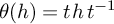




Let
$\mathbb {X}$
 be a graph of groups whose underlying graph we will denote by X and let
$\pi = \pi _1(\mathbb {X})$
be a graph of groups whose underlying graph we will denote by X and let
$\pi = \pi _1(\mathbb {X})$
 be its fundamental group. We will recall the construction of the Bass-Serre tree
$\widetilde {X}$
be its fundamental group. We will recall the construction of the Bass-Serre tree
$\widetilde {X}$
 of
$\mathbb {X}$
of
$\mathbb {X}$
 whose vertices are

while its edges are given by

where
$\mathrm {Edge}_+(X)$
 is a fixed orientation of the edges of X. In the definition above we are including only the edges of a fixed orientation of
$\widetilde {X}$
is a fixed orientation of the edges of X. In the definition above we are including only the edges of a fixed orientation of
$\widetilde {X}$
 induced by the orientation of X. We can define the endpoint of each edge as follows

where
$g_{y}$
 is the image of y under the canonical projection from
$F(\mathbb {X})$
is the image of y under the canonical projection from
$F(\mathbb {X})$
 to
$\pi _1(\mathbb {X};T)$
to
$\pi _1(\mathbb {X};T)$
 . The group
$\pi $
. The group
$\pi $
 acts on
$\widetilde {X}$
acts on
$\widetilde {X}$
 by left multiplication. The Bass-Serre tree construction also allows us to produce actions on trees for the fundamental group of any graph of groups. We will exploit this to obtain examples of Fourier multipliers satisfying Cotlar’s identity.
We are ready to prove the main theorem of this section.
Proof of Theorem D
For (i), take
$h \in \mathrm {G}_{x_0}$
 ; then it is immediate that
$m(g h)=m(g)$
; then it is immediate that
$m(g h)=m(g)$
 . Therefore, it is enough to prove the identity for
$g, h \not \in \mathrm {G}_{x_0}$
. Therefore, it is enough to prove the identity for
$g, h \not \in \mathrm {G}_{x_0}$
 . Assume that
$m(gh) \neq m(g)$
. Assume that
$m(gh) \neq m(g)$
 , since otherwise the identity holds. Let us write g in its normal form
$g=r_0 \, y_1 \, r_1 \, y_2 \, r_2 \cdots y_{n} \, r_n$
, since otherwise the identity holds. Let us write g in its normal form
$g=r_0 \, y_1 \, r_1 \, y_2 \, r_2 \cdots y_{n} \, r_n$
 with
$r_0 \in g_0 \cdot \mathrm {H}_{\bar y_1}^{\bar y_1}$
with
$r_0 \in g_0 \cdot \mathrm {H}_{\bar y_1}^{\bar y_1}$
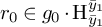 . Since
$m(gh) \neq m(g)$
. Since
$m(gh) \neq m(g)$
 , h must admit a normal form
$b = r_n^{-1} y_n^{-1} \cdots y_1^{-1}r$
, h must admit a normal form
$b = r_n^{-1} y_n^{-1} \cdots y_1^{-1}r$
 with
$r=r_0^{-1}\cdot r'$
with
$r=r_0^{-1}\cdot r'$
 for some
$r' \in g_0' \cdot \mathrm {H}_{\bar y_1}^{\bar y_1}$
for some
$r' \in g_0' \cdot \mathrm {H}_{\bar y_1}^{\bar y_1}$
 . Here
$g_0, \, g_0' \in \mathrm {G}_{x_0}$
. Here
$g_0, \, g_0' \in \mathrm {G}_{x_0}$
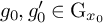 and
$g_0^{-1}g_0' \notin \mathrm {H}_{\bar y_1}^{\bar y_1}$
and
$g_0^{-1}g_0' \notin \mathrm {H}_{\bar y_1}^{\bar y_1}$
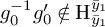 . Moreover, since
$ r_n^{-1} y_n^{-1} \cdots y_1^{-1}r_0^{-1}$
. Moreover, since
$ r_n^{-1} y_n^{-1} \cdots y_1^{-1}r_0^{-1}$
 is a normal form of
$g^{-1}$
is a normal form of
$g^{-1}$
 , by the definition of m, it is clear that
$m(g^{-1})=m(h)$
, by the definition of m, it is clear that
$m(g^{-1})=m(h)$
 . For (ii), notice that the left action
$\mathrm {G}_{x_0} \curvearrowright \mathrm {G}_{x_0} / \mathrm {H}_{\bar {y}}^{\bar {y}}$
. For (ii), notice that the left action
$\mathrm {G}_{x_0} \curvearrowright \mathrm {G}_{x_0} / \mathrm {H}_{\bar {y}}^{\bar {y}}$
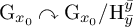 is transitive for each y, therefore a left
$\mathrm {G}_{x_0}$
is transitive for each y, therefore a left
$\mathrm {G}_{x_0}$
 -invariant function has to be constant in each of the elements of the disjoint union W.
Observe that, by the definition of the Bass-Serre tree of
$\mathbb {X}$
 in equation (5.2), the set of edges in
$\widetilde {X}$
in equation (5.2), the set of edges in
$\widetilde {X}$
 connected to the vertex
$\widetilde {x}_0 = e \cdot \mathrm {G}_{x_0} \in \mathrm {Vert}(\widetilde {X})$
connected to the vertex
$\widetilde {x}_0 = e \cdot \mathrm {G}_{x_0} \in \mathrm {Vert}(\widetilde {X})$
 is given, up to orientation, by the disjoint union of
$\mathrm {G}_{x_0} / \mathrm {H}_{\bar {y}}^{\bar {y}}$
is given, up to orientation, by the disjoint union of
$\mathrm {G}_{x_0} / \mathrm {H}_{\bar {y}}^{\bar {y}}$
 , where, again, y runs over every edge in X starting with
$x_0$
, where, again, y runs over every edge in X starting with
$x_0$
 . This already establishes that the functions depending only on the initial segment and the functions that are constant on the connected components of
$\widetilde {X} \setminus \{\widetilde x_0\}$
. This already establishes that the functions depending only on the initial segment and the functions that are constant on the connected components of
$\widetilde {X} \setminus \{\widetilde x_0\}$
 are in a natural and bijective correspondence. The following proposition, whose proof is immediate, asserts that m falls into Model 1. This provides an alternative proof of Theorem D via Proposition 3.1.(i).
Proposition 5.1. Let
$\pi = \pi _1 (\mathbb {X},x_0)$
 be the fundamental group of a connected graph of groups
$\mathbb {X}$
be the fundamental group of a connected graph of groups
$\mathbb {X}$
 and let
$\widetilde {X}$
and let
$\widetilde {X}$
 be its Bass-Serre tree.
-
(i) Every symbol $m: \pi \to \mathbb {C}$
depending on the first segment satisfies $$\begin{align*}m( g ) = \widetilde{m}(g \cdot \widetilde{x}_0), \end{align*}$$where $\widetilde {m}: \widetilde {X} \to \mathbb {C}$
is the function constant over the connected components of
$\widetilde {X} \setminus \{\widetilde {x}_0\}$
that is naturally associated to (1.6) and
$\widetilde {x}_0$
is a vertex of
$\widetilde {X}$
labelled by
$\mathrm {G}_{x_0}$
.
-
(ii) If furthermore m depends only on the edge of the starting segment, then $\widetilde {m}:\widetilde {X} \setminus \{\widetilde {x}_0\} \to \mathbb {C}$
has the same value over any two connected components
$\widetilde X_\alpha $
and
$\widetilde X_\beta $
such that
$r \cdot \widetilde X_\alpha = \widetilde X_\beta $
, for some
$r \in \mathrm {G}_{x_0}$
.





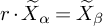

In the case in which
$\mathrm {G}_{x_0}$
 is Abelian, the more restrictive condition that
$m:\pi \to \mathbb {C}$
is Abelian, the more restrictive condition that
$m:\pi \to \mathbb {C}$
 depends on the initial edge can be removed and a multiplier theorem still holds for symbols depending on the starting segment. Let m be a symbol depending on the starting segment and
$\widetilde {m}: W_{x_0} \to \mathbb {C}$
depends on the initial edge can be removed and a multiplier theorem still holds for symbols depending on the starting segment. Let m be a symbol depending on the starting segment and
$\widetilde {m}: W_{x_0} \to \mathbb {C}$
 be its lift to the space of initial segments defined in (1.5). We will denote by
$\widetilde {m}_y$
be its lift to the space of initial segments defined in (1.5). We will denote by
$\widetilde {m}_y$
 the restriction of
$\widetilde {m}$
the restriction of
$\widetilde {m}$
 to
$\mathrm {G}_{x_0}/\mathrm {H}_{\bar {y}}^{\bar {y}}$
to
$\mathrm {G}_{x_0}/\mathrm {H}_{\bar {y}}^{\bar {y}}$
 . We have the following result.
Theorem 5.2. Let
$\pi =\pi _1(\mathbb {X},x_0)$
 be the fundamental group of a graph of groups with
$\mathrm {G}_{x_0}$
be the fundamental group of a graph of groups with
$\mathrm {G}_{x_0}$
 Abelian. In order to lighten the notation, let us denote
$\mathrm {G}_{x_0}/\mathrm {H}_{\bar {y}}^{\bar {y}}$
Abelian. In order to lighten the notation, let us denote
$\mathrm {G}_{x_0}/\mathrm {H}_{\bar {y}}^{\bar {y}}$
 by
$\mathrm {G}_y$
by
$\mathrm {G}_y$
 . For each
$y \in \mathrm {Edge}(X)$
. For each
$y \in \mathrm {Edge}(X)$
 with
$\mathrm {o}(y) = x_0$
with
$\mathrm {o}(y) = x_0$
 and each character
$\chi : \mathrm {G}_y \to \mathbb {T}$
and each character
$\chi : \mathrm {G}_y \to \mathbb {T}$
 we define the multiplier
$\sigma _{y, \, \chi }$
we define the multiplier
$\sigma _{y, \, \chi }$
 given by
$\sigma _{y, \, \chi }(g) = \chi (r_0 \, \mathrm {H}_{\bar {y}}^{\bar {y}})$
given by
$\sigma _{y, \, \chi }(g) = \chi (r_0 \, \mathrm {H}_{\bar {y}}^{\bar {y}})$
 , whenever g is represented by a word starting by
$r_0 \, y$
, whenever g is represented by a word starting by
$r_0 \, y$
 , and
$0$
, and
$0$
 otherwise. The following results hold
-
(i) The map $\rho _{y}: L_p(\mathcal {L} \pi ) \to L_p(\widehat {\mathrm {G}}_y;L_p(\mathcal {L} \pi ))$
, defined by
$f \mapsto (T_{\sigma _{y,\chi }}(f))_{\chi \in \widehat {\mathrm {G}}_y}$
satisfies $$\begin{align*}\| f \|_p \leq \big\| \rho_{y}(f) \big\|_{L_p(\widehat{\mathrm{G}}_y;L_p(\mathcal{L} \pi))} \lesssim \Big( \frac{p^2}{p-1} \Big)^\beta \| f \|_{p}, \;\; \text{ where } \beta = \log_2(1+\sqrt{2}), \end{align*}$$
-
(ii) For a general symbol $m: \pi \to \mathbb {C}$
depending on the starting segment, it holds that $$\begin{align*}\big\| T_m: L_p(\mathcal{L} \pi) \to L_p(\mathcal{L} \pi) \big\| \lesssim \Big( \frac{p^2}{p-1} \Big)^\beta \, \max_{\mathrm{o}(y) = x_0 } \Big\{ \big\| T_{\tilde{m}_y}: L_p(\widehat{\mathrm{G}}_y) \to L_p(\widehat{\mathrm{G}}_y) \big\|_{\mathrm{cb}} \Big\}. \end{align*}$$




Proof. The proof is almost immediate. For (i) first notice that
$m_{y,\chi }$
 depends on the starting segment and that, given
$a \in \mathrm {G}_{x_0}$
depends on the starting segment and that, given
$a \in \mathrm {G}_{x_0}$
 ,
$\sigma _{y,\chi }$
,
$\sigma _{y,\chi }$
 satisfies that
$\sigma _{y,\chi }(a \, g ) = \chi (a) \, \sigma _{y,\chi }(g)$
satisfies that
$\sigma _{y,\chi }(a \, g ) = \chi (a) \, \sigma _{y,\chi }(g)$
 . Thus, since it satisfies (Cotla ^r) relative to
$\mathrm {G}_{x_0}$
. Thus, since it satisfies (Cotla ^r) relative to
$\mathrm {G}_{x_0}$
 , by Remark 2.6 we have that it is a bounded multiplier in
$L_p$
, by Remark 2.6 we have that it is a bounded multiplier in
$L_p$
 for
$1<p<\infty $
for
$1<p<\infty $
 satisfying the bound (1.1) in Theorem A. The fact that
$\widehat {\mathrm {G}}_y$
satisfying the bound (1.1) in Theorem A. The fact that
$\widehat {\mathrm {G}}_y$
 is compact implies that
$\rho _y$
is compact implies that
$\rho _y$
 is bounded with the same bound as
$T_{\sigma _{y,\chi }}$
is bounded with the same bound as
$T_{\sigma _{y,\chi }}$
 . For the lower bound, notice that, since the Haar measure of
$\widehat {\mathrm {G}}_y$
. For the lower bound, notice that, since the Haar measure of
$\widehat {\mathrm {G}}_y$
 is a probability measure,
${\mathbf {1}}_{\widehat {\mathrm {G}}_y}$
is a probability measure,
${\mathbf {1}}_{\widehat {\mathrm {G}}_y}$
 is of norm one on
$L_{p'}(\widehat {\mathrm {G}}_y)$
is of norm one on
$L_{p'}(\widehat {\mathrm {G}}_y)$
 . But evaluating against it gives

This shows that
$\rho _y$
 is a quasi-isometry, which gives (i). For (ii), just notice that if m is a symbol depending on the starting segment and that is
$0$
is a quasi-isometry, which gives (i). For (ii), just notice that if m is a symbol depending on the starting segment and that is
$0$
 outside
$\mathrm {G}_y$
outside
$\mathrm {G}_y$
 , then the following diagram commutes

and together with point (i), this yields the result. In the general case of m depending on the starting segment, we can decompose it as a sum of symbols
$\widetilde {m}{|}_{\mathrm {G}_y}$
 and build a direct sum map

by taking
$\rho _y$
 in each of the components.
Now, we have all the tools required to illustrate our theory with the examples.
Examples: Amalgamated free products. This first example is already known, but our proof gives a concise geometric interpretation of it. Let
$\{\mathrm {G}_i: i \geq 1 \}$
 be a family of groups and A a common subgroup. Let us denote the injective homomorphisms by
$\alpha _i : A \rightarrow \mathrm {G}_i$
be a family of groups and A a common subgroup. Let us denote the injective homomorphisms by
$\alpha _i : A \rightarrow \mathrm {G}_i$
 , for
$i \geq 1$
, for
$i \geq 1$
 . Now, consider the graph of groups
$\mathbb {X}$
. Now, consider the graph of groups
$\mathbb {X}$
 in Figure 7, whose underlying tree X connects the point
$x_0$
in Figure 7, whose underlying tree X connects the point
$x_0$
 , with
$\mathrm {G}_{x_0} = A$
, with
$\mathrm {G}_{x_0} = A$
 , with the points
$x_i$
, with the points
$x_i$
 ,
$i \geq 1$
,
$i \geq 1$
 , whose groups are
$\mathrm {G}_i$
, whose groups are
$\mathrm {G}_i$
 . Meanwhile, the groups on the edges
$y_i$
. Meanwhile, the groups on the edges
$y_i$
 are all isomorphic to A with the embedding into
$\mathrm {G}_{x_0} = A$
are all isomorphic to A with the embedding into
$\mathrm {G}_{x_0} = A$
 being the identity map and the embedding into
$\mathrm {G}_i$
being the identity map and the embedding into
$\mathrm {G}_i$
 being
$\alpha _i$
being
$\alpha _i$
 .
.
Graph of groups for the amalgamated free product.

In this case, we have that
$\pi = \pi _1(\mathbb {X},x_0)$
 is the free product of
$\{\mathrm {G}_i : i \geq 1 \}$
is the free product of
$\{\mathrm {G}_i : i \geq 1 \}$
 with A as the amalgam
$\pi = {{{{{\ast}}}}_{i, \, A}} \mathrm {G}_i$
with A as the amalgam
$\pi = {{{{{\ast}}}}_{i, \, A}} \mathrm {G}_i$
 , see [Reference Serre79, Theorem 9]. Functions
$m: \pi \to \mathbb {C}$
, see [Reference Serre79, Theorem 9]. Functions
$m: \pi \to \mathbb {C}$
 that depend on the starting edge in this context are given by the span of
$\{L_i\}_{i \geq 1}$
that depend on the starting edge in this context are given by the span of
$\{L_i\}_{i \geq 1}$
 , where each
$L_i$
, where each
$L_i$
 is the Fourier multiplier associated to the characteristic function of the words starting by
$a \, s_{i}$
is the Fourier multiplier associated to the characteristic function of the words starting by
$a \, s_{i}$
 , where
$s_{i} \in \mathrm {G}_i$
, where
$s_{i} \in \mathrm {G}_i$
 . These operators are an example of the free Hilbert transforms that have been studied in the pioneering work of Mei and Ricard [Reference Mei and Ricard55]. Note that free groups can be obtained from other graphs of groups. Let us pick the free group of two generators
$\mathbb {F}_2$
. These operators are an example of the free Hilbert transforms that have been studied in the pioneering work of Mei and Ricard [Reference Mei and Ricard55]. Note that free groups can be obtained from other graphs of groups. Let us pick the free group of two generators
$\mathbb {F}_2$
 for simplicity. We can represent
$\mathbb {F}_2$
for simplicity. We can represent
$\mathbb {F}_2$
 as the fundamental group of the graph of groups
$\mathbb {X}$
as the fundamental group of the graph of groups
$\mathbb {X}$
 given by two vertices
$\{x_0, x_1\}$
given by two vertices
$\{x_0, x_1\}$
 whose associated groups are isomorphic to
$\mathbb {Z}$
whose associated groups are isomorphic to
$\mathbb {Z}$
 and joined by a single edge with trivial group in it.
Let us denote the generator associated to
$x_0$
 by a and the generator associated to
$x_1$
by a and the generator associated to
$x_1$
 by b. Since
$\mathbb {Z} =\langle a \rangle $
by b. Since
$\mathbb {Z} =\langle a \rangle $
 is Abelian, we can apply Theorem 5.2. Indeed, functions depending on the starting segment are of the form
$m( s_1^{n_1} \, s_2^{n_2} \, \cdots \, s_r^{n_r}) = \widetilde {m}(n_1)$
is Abelian, we can apply Theorem 5.2. Indeed, functions depending on the starting segment are of the form
$m( s_1^{n_1} \, s_2^{n_2} \, \cdots \, s_r^{n_r}) = \widetilde {m}(n_1)$
 if
$s_1 =a$
if
$s_1 =a$
 and
$0$
and
$0$
 otherwise. Changing the roles of
$x_0$
otherwise. Changing the roles of
$x_0$
 and
$x_1$
and
$x_1$
 and combining the two multipliers obtained, we get symbols of the form

Since m above is the sum of two symbols satisfying the hypothesis of Theorem 5.2(ii), we have that

where
$p'$
 is the conjugate exponent
$\tfrac 1{p}+\tfrac 1{p'}=1$
is the conjugate exponent
$\tfrac 1{p}+\tfrac 1{p'}=1$
 . With this, we partially recover the multiplier theorems for initial segments of the free group in [Reference Mei, Ricard and Xu56]. Our approach has the advantage of giving a geometric interpretation as follows. Consider the Bass-Serre tree
$\widetilde {X}$
. With this, we partially recover the multiplier theorems for initial segments of the free group in [Reference Mei, Ricard and Xu56]. Our approach has the advantage of giving a geometric interpretation as follows. Consider the Bass-Serre tree
$\widetilde {X}$
 of this graph of groups, see Figure 8; it is easy to see that group elements in
$\mathbb {F}_2$
of this graph of groups, see Figure 8; it is easy to see that group elements in
$\mathbb {F}_2$
 can only map pink vertices to pink vertices and blue ones to blue ones. Denote the set containing the blue vertices in the first layer and the pink vertex labeled by
$\mathbb {Z}$
can only map pink vertices to pink vertices and blue ones to blue ones. Denote the set containing the blue vertices in the first layer and the pink vertex labeled by
$\mathbb {Z}$
 in the middle by
$B_1$
in the middle by
$B_1$
 . It is straightforward to realize that any function on
$\widetilde {X}$
. It is straightforward to realize that any function on
$\widetilde {X}$
 that is constant along the connected components of
$\widetilde {X} \setminus B_1$
that is constant along the connected components of
$\widetilde {X} \setminus B_1$
 induces a symbol of the form (5.3).
Graph of groups whose fundamental group is
$\mathbb {F}_2$
 (in the corner) and its Bass-Serre tree. For readability, we have omitted branches going from the root towards vertices labeled
$a^{k} \mathbb {Z}$
(in the corner) and its Bass-Serre tree. For readability, we have omitted branches going from the root towards vertices labeled
$a^{k} \mathbb {Z}$
 with
$k \leq 0$
with
$k \leq 0$
 .
.

Figure 8 Long description
The main structure is a tree diagram. At the center is a large pink circular node labeled with the symbol for integers Z.
Moving outward from this central root, several lines connect to a second layer of light blue nodes. These nodes are labeled from left to right as a Z, a super 2 Z, a super 3 Z, and a super j Z.
A third layer of smaller pink nodes branches from the second layer. From the node a Z, branches lead to nodes labeled a b Z, a b super 2 Z, and a b super 3 Z. From the node a super 2 Z, branches lead to a super 2 b Z and a super 2 b super 2 Z. From the node a super j Z, branches lead to a super i b Z and a super i b super 2 Z.
A fourth layer of light blue nodes branches from the pink node a b Z, with labels a b a Z and a b a super 2 Z.
Throughout the tree, dashed lines and ellipses indicate omitted branches continuing into higher powers.
In the bottom right corner, a separate small graph consists of two nodes connected by a single horizontal line. The left node is pink and the right node is light blue, both labeled with the symbol for integers Z.
The fact that the starting letter induces bounded multipliers suggests the enticing possibility of simultaneously generalizing our results for the starting segment in Theorem D and 5.2 and the main result in [Reference Mei, Ricard and Xu56] to multipliers depending on the starting k-word of the normal form in the context of graphs of groups.
Examples: HNN extensions. Suppose
$\mathrm {H}_1$
 and
$\mathrm {H}_2 \subseteq \mathrm {G}$
and
$\mathrm {H}_2 \subseteq \mathrm {G}$
 are two subgroups isomorphic under
$\theta : \mathrm {H}_1 \to \mathrm {H}_2$
are two subgroups isomorphic under
$\theta : \mathrm {H}_1 \to \mathrm {H}_2$
 and let
$\pi $
and let
$\pi $
 be the HNN-extension of
$\mathrm {G}$
be the HNN-extension of
$\mathrm {G}$
 relative to
$\theta $
relative to
$\theta $
 , given in (5.1). Observe that the HNN-extension can be written as
$\pi = H \rtimes T$
, given in (5.1). Observe that the HNN-extension can be written as
$\pi = H \rtimes T$
 , the semi-direct product of the infinite cyclic group T generated by t and the normal subgroup H generated by
$t^n \mathrm {G} t^{-n}$
, the semi-direct product of the infinite cyclic group T generated by t and the normal subgroup H generated by
$t^n \mathrm {G} t^{-n}$
 ,
$n \in \mathbb {Z}$
,
$n \in \mathbb {Z}$
 . In particular,
$\pi $
. In particular,
$\pi $
 has a quotient isomorphic to
$\mathbb {Z}$
has a quotient isomorphic to
$\mathbb {Z}$
 .
.
We have already seen, see Figure 6, that
$\pi = \pi _1(\mathbb {X},x_0)$
 is the fundamental group of a graph of groups based on a single loop. By the definition of fundamental group, every element of
$\pi $
is the fundamental group of a graph of groups based on a single loop. By the definition of fundamental group, every element of
$\pi $
 is represented by a word
$r_0, t^{e_1} \, r_1 \, \cdots \, t^{e_k} \,, r_k$
is represented by a word
$r_0, t^{e_1} \, r_1 \, \cdots \, t^{e_k} \,, r_k$
 with
$k\geq 0$
with
$k\geq 0$
 ,
$e_i=\pm 1$
,
$e_i=\pm 1$
 and
$r_i \in \mathrm {G}$
and
$r_i \in \mathrm {G}$
 . A word in this form will be reduced if it contains neither a substring of the form
$t a t^{-1}$
. A word in this form will be reduced if it contains neither a substring of the form
$t a t^{-1}$
 with
$ a \in \mathrm {H}_1$
with
$ a \in \mathrm {H}_1$
 nor one of the form
$t^{-1} b t$
nor one of the form
$t^{-1} b t$
 with
$b \in \mathrm {H}_2$
with
$b \in \mathrm {H}_2$
 . Fix coset representatives of
$\mathrm {G}/\mathrm {H}_1$
. Fix coset representatives of
$\mathrm {G}/\mathrm {H}_1$
 and
$\mathrm {G}/\mathrm {H}_2$
and
$\mathrm {G}/\mathrm {H}_2$
 ; for any
$g\in \pi $
; for any
$g\in \pi $
 , there exists a unique reduced word such that

with
$r_0 \in \mathrm {G}$
 ,
$r_i \in \mathrm {G}/\mathrm {H}_1$
,
$r_i \in \mathrm {G}/\mathrm {H}_1$
 if
$e_i=1$
if
$e_i=1$
 , and
$r_i \in \mathrm {G}/\mathrm {H}_2$
, and
$r_i \in \mathrm {G}/\mathrm {H}_2$
 if
$e_i=-1$
if
$e_i=-1$
 . We are going to give two algebraic forms for Fourier multipliers satisfying (Cotlar𝔼
⊥), one falling within Model 1 and another within Model 2 by considering the action of the HNN-extension
$\pi $
. We are going to give two algebraic forms for Fourier multipliers satisfying (Cotlar𝔼
⊥), one falling within Model 1 and another within Model 2 by considering the action of the HNN-extension
$\pi $
 on its Bass-Serre tree
$\widetilde {X}$
on its Bass-Serre tree
$\widetilde {X}$
 by left multiplication. For the first one, we choose the root
$\widetilde {x}_0$
by left multiplication. For the first one, we choose the root
$\widetilde {x}_0$
 to be the vertex labeled by
$\mathrm {G}$
to be the vertex labeled by
$\mathrm {G}$
 . Note that if we set the orientation
$\mathrm {Edge}_+(X)=\{t\}$
. Note that if we set the orientation
$\mathrm {Edge}_+(X)=\{t\}$
 , then in the induced orientation of
$\widetilde {X}$
, then in the induced orientation of
$\widetilde {X}$
 there are
$[\mathrm {G}: \mathrm {H}_2]$
there are
$[\mathrm {G}: \mathrm {H}_2]$
 many edges starting at
$\widetilde {x}_0$
many edges starting at
$\widetilde {x}_0$
 and
$[\mathrm {G}: \mathrm {H}_1]$
and
$[\mathrm {G}: \mathrm {H}_1]$
 many edges ending in
$\widetilde {x}_0$
many edges ending in
$\widetilde {x}_0$
 . It is immediate that a function
$m: \pi \to \mathbb {C}$
. It is immediate that a function
$m: \pi \to \mathbb {C}$
 depends on the starting segment iff there is a function
$\widetilde {m}: ( \mathrm {G}/\mathrm {H}_1 ) \sqcup ( \mathrm {G}/\mathrm {H}_2) \to \mathbb {C}$
depends on the starting segment iff there is a function
$\widetilde {m}: ( \mathrm {G}/\mathrm {H}_1 ) \sqcup ( \mathrm {G}/\mathrm {H}_2) \to \mathbb {C}$
 such that

where
$\widetilde {m}_i$
 is the restriction of
$\widetilde {m}$
is the restriction of
$\widetilde {m}$
 to
$\mathrm {G}/\mathrm {H}_i$
to
$\mathrm {G}/\mathrm {H}_i$
 for
$i \in \{1,2\}$
for
$i \in \{1,2\}$
 and g is equal to its normal form like in (5.4). By Proposition 5.1, we have that m is left
$\mathrm {G}$
and g is equal to its normal form like in (5.4). By Proposition 5.1, we have that m is left
$\mathrm {G}$
 -invariant if and only if it depends only on the first edge in the normal form (5.4), which can only be t or
$t^{-1}$
-invariant if and only if it depends only on the first edge in the normal form (5.4), which can only be t or
$t^{-1}$
 in our setting, ie:

Observe that, if
$\mathrm {G}$
 is Abelian, we can deal with the boundedness of (5.5).
Now, we can use the definition in Model 2 to the action
$\pi \curvearrowright \widetilde {X}$
 . Choose
$\widetilde {x}_0$
. Choose
$\widetilde {x}_0$
 as the root and let
$\widetilde {X}_0 \subseteq \widetilde {X}$
as the root and let
$\widetilde {X}_0 \subseteq \widetilde {X}$
 be the connected component separated from the root by the edge
$\mathrm {H}_1$
be the connected component separated from the root by the edge
$\mathrm {H}_1$
 . It is easy to check the vertices in the connected component of
$\mathrm {H}_2$
. It is easy to check the vertices in the connected component of
$\mathrm {H}_2$
 always take the form
$g\cdot \mathrm {G}$
always take the form
$g\cdot \mathrm {G}$
 with the expression (5.4) of g starting with t. Hence we get the following symbol
$\varphi : \pi \to \mathbb {C}$
with the expression (5.4) of g starting with t. Hence we get the following symbol
$\varphi : \pi \to \mathbb {C}$
 :
:

where
$D_1$
 and
$D_2$
and
$D_2$
 are two different constants.
Corollary 5.3. Let
$\pi $
 be the HNN extension of
$\mathrm {G}$
be the HNN extension of
$\mathrm {G}$
 with respect to
$\theta $
with respect to
$\theta $
 as before.
-
(i) Let $m: \pi \to \mathbb {C}$
be like in (5.6). Since m depends on the starting edge,
$T_m$
is
$L_p$
-bounded for
$1 < p < \infty $
and satisfies bound (1.1) by Theorem D. -
(ii) If $\mathrm {G}$
is Abelian, and the symbol m in (5.5) lifts to
$\widetilde {m}: (\mathrm {G}/\mathrm {H}_1) \sqcup (\mathrm {G}/\mathrm {H}_2) \to \mathbb {C}$
, then, by Theorem 5.2, it holds that $$\begin{align*}\big\| T_m: L_p(\mathcal{L} \pi) \to L_p(\mathcal{L} \pi) \big\| \lesssim \Big( \frac{p^2}{p-1} \Big)^\beta \, \max_{i=1,2} \Big\{ \big\| T_{m_{i}}: L_p(\widehat{\mathrm{G}/\mathrm{H}_i}) \to L_p(\widehat{\mathrm{G}/\mathrm{H}_i}) \big\|_{\mathrm{cb}} \Big\}. \end{align*}$$
-
(iii) Let $\varphi : \pi \to \mathbb {C}$
be as in (5.7). Then
$T_\varphi $
, by Theorem 2.4, satisfies (Cotlar𝔼
⊥) relative to
$\mathrm {H}_2 \subseteq \mathrm {G}$
and is left
$\mathcal {L} \mathrm {H}_2$
-modular. Thus
$T_\varphi $
is bounded in
$L_p$
with bound (1.1).





The result above can be illustrated in the particular case of the Baumslag-Solitar group

which can be seen as a HNN extension of
$\mathbb {Z} = \langle r \rangle $
 with respect to the map
$\theta $
with respect to the map
$\theta $
 , which sends
$r^{m k} \mapsto r^{n k}$
, which sends
$r^{m k} \mapsto r^{n k}$
 and establishes an isomorphism between the subgroups
$m\mathbb {Z}$
and establishes an isomorphism between the subgroups
$m\mathbb {Z}$
 and
$n\mathbb {Z} \subseteq \mathbb {Z}$
and
$n\mathbb {Z} \subseteq \mathbb {Z}$
 . It holds that
$\mathbb {Z} / n\mathbb {Z} \cong \mathbb {Z}_n$
. It holds that
$\mathbb {Z} / n\mathbb {Z} \cong \mathbb {Z}_n$
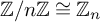 and
$\mathbb {Z} / m \mathbb {Z} \cong \mathbb {Z}_m$
and
$\mathbb {Z} / m \mathbb {Z} \cong \mathbb {Z}_m$
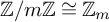 . We can take representatives
$\{0, \, 1, \, \dots \, n - 1\}$
. We can take representatives
$\{0, \, 1, \, \dots \, n - 1\}$
 and
$\{0, \, 1, \, \dots \, m - 1\}$
and
$\{0, \, 1, \, \dots \, m - 1\}$
 of the quotients. The unique normal form of g is given by

if
$e_{j}=1$
 , then
$k_j\in \mathbb {Z} / {m\mathbb {Z}}$
, then
$k_j\in \mathbb {Z} / {m\mathbb {Z}}$
 for
$j \geq 1$
for
$j \geq 1$
 . If
$e_{j}=-1$
. If
$e_{j}=-1$
 , then
$k_j \in \mathbb {Z} / {n\mathbb {Z}}$
, then
$k_j \in \mathbb {Z} / {n\mathbb {Z}}$
 for
$j \geq 1$
for
$j \geq 1$
 . Multipliers that depend on the starting segment
$\varphi : \pi \to \mathbb {C}$
. Multipliers that depend on the starting segment
$\varphi : \pi \to \mathbb {C}$
 lift to a function
$\widetilde {\varphi }: (\mathbb {Z}/n\mathbb {Z}) \sqcup (\mathbb {Z}/m\mathbb {Z}) \to \mathbb {C}$
lift to a function
$\widetilde {\varphi }: (\mathbb {Z}/n\mathbb {Z}) \sqcup (\mathbb {Z}/m\mathbb {Z}) \to \mathbb {C}$
 as in (5.5). Using the fact that
$\mathbb {Z}$
as in (5.5). Using the fact that
$\mathbb {Z}$
 is Abelian and Corollary 5.3 gives

where we have also used the fact that the multiplier norm of
$\varphi : \mathbb {Z}/\ell \mathbb {Z} \to \mathbb {C}$
 on
$L_p(\mathbb {Z}/\ell \mathbb {Z})$
on
$L_p(\mathbb {Z}/\ell \mathbb {Z})$
 is bounded by
$\ell ^{|\frac {1}{2}-\frac {1}{p}|} \| \varphi \|_\infty $
is bounded by
$\ell ^{|\frac {1}{2}-\frac {1}{p}|} \| \varphi \|_\infty $
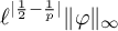 . Now, let us explore multipliers on
$\mathrm {BS}(n,m)$
. Now, let us explore multipliers on
$\mathrm {BS}(n,m)$
 coming from Model 2 as in (5.7). Let
$\mathbb {X}$
coming from Model 2 as in (5.7). Let
$\mathbb {X}$
 be the single loop graph of groups associated with
$\mathrm {BS}(n,m)$
be the single loop graph of groups associated with
$\mathrm {BS}(n,m)$
 and
$\widetilde {X}$
and
$\widetilde {X}$
 be its Bass-Serre tree depicted in Figure 9. The two directions of the loop give us the two subgroups
$m\mathbb {Z}, \, n\mathbb {Z}$
be its Bass-Serre tree depicted in Figure 9. The two directions of the loop give us the two subgroups
$m\mathbb {Z}, \, n\mathbb {Z}$
 , and by definition of the Bass-Serre tree you get that
$\widetilde {X} \setminus \{\widetilde {x}_0\}$
, and by definition of the Bass-Serre tree you get that
$\widetilde {X} \setminus \{\widetilde {x}_0\}$
 has
$n + m$
has
$n + m$
 connected components, see Figure 9. Now, we select the connected component of the vertex
$t \mathrm {G}$
connected components, see Figure 9. Now, we select the connected component of the vertex
$t \mathrm {G}$
 . The symbol obtained has a value that depends on whether the normal form (5.8) starts with t or not.
Graph of groups whose fundamental group is the Baumslag-Solitar group (in the corner) and its Bass-Serre tree. Here
$\mathrm {G} = \mathbb {Z}$
 and
$\mathrm {H}_1 = n\mathbb {Z} \subseteq \mathbb {Z}$
and
$\mathrm {H}_1 = n\mathbb {Z} \subseteq \mathbb {Z}$
 .
.

Figure 9 Long description
The diagram illustrates the Bass-Serre tree for a group G. At the center is a large circular node labeled G. Radiating from this center are several blue edges connecting to smaller circular nodes. Moving clockwise from the top-left: an edge labeled t inverse H sub 1 connects to node t inverse G; an edge labeled r t inverse H sub 1 connects to node r t inverse G; an ellipsis indicates further nodes; and an edge labeled r super n minus 1 t inverse H sub 1 connects to node r super n minus 1 t inverse G. In the bottom-right quadrant, an edge labeled r super m minus 1 H sub 1 connects to node r super m minus 1 t G. In the bottom-center, an edge labeled r H sub 1 connects to node r t G. In the bottom-left, an edge labeled H sub 1 connects to node t G. This t G node is the root of a sub-tree highlighted by a pink shaded background. From t G, three edges descend: t H sub 1 to node t squared G, t r H sub 1 to node t r t G, and t r super m minus 1 H sub 1 to node t r super m minus 1 t G, with an ellipsis between them. In the bottom-right corner, separate from the tree, is a graph of groups consisting of a single node G with a blue self-loop edge.
Observe that
$\mathrm {BS}(n,m)$
 has an Abelian quotient
$q: \mathrm {BS}(n,m) \to \mathbb {Z}$
has an Abelian quotient
$q: \mathrm {BS}(n,m) \to \mathbb {Z}$
 given by killing the ‘base group’
$\langle r\rangle $
given by killing the ‘base group’
$\langle r\rangle $
 , i.e.
$q(t)=1$
, i.e.
$q(t)=1$
 and
$q(r)=0$
and
$q(r)=0$
 . Composing q with a sign gives an example of a multiplier satisfying Cotlar’s identity. Nevertheless, the multipliers studied above, (5.5) and (5.7) do not arise from the signs of this Abelian quotient
$ \mathbb {Z}$
. Composing q with a sign gives an example of a multiplier satisfying Cotlar’s identity. Nevertheless, the multipliers studied above, (5.5) and (5.7) do not arise from the signs of this Abelian quotient
$ \mathbb {Z}$
 . The following was pointed out to us by the referee.
Remark 5.4. When m and n have a common factor
$d\in \mathbb {Z}$
 ,
$\mathrm {BS}(n,m)$
,
$\mathrm {BS}(n,m)$
 can be written as an amalgamated free product

where
$\mathrm {BS}(\frac {n}{d},\frac {m}{d})=\langle s, t \, \big {|} \,ts^{\frac {m}{d}}t^{-1}=s^{\frac {n}{d}} \rangle $
 , the amalgam
$\mathbb {Z}$
, the amalgam
$\mathbb {Z}$
 is identified with
$\langle s\rangle $
is identified with
$\langle s\rangle $
 in
$\mathrm {BS}(\frac {n}{d},\frac {m}{d})$
in
$\mathrm {BS}(\frac {n}{d},\frac {m}{d})$
 and with
$d\mathbb {Z}$
and with
$d\mathbb {Z}$
 in
$\mathbb {Z}$
in
$\mathbb {Z}$
 . Then in this case we also have a free Hilbert transform on
$\mathrm {BS}(n,m)$
. Then in this case we also have a free Hilbert transform on
$\mathrm {BS}(n,m)$
 whose symbol takes the form:

which is different from the multiplier formulas in (5.6) and (5.7).
Examples with Serre’s Property (FA). We will present here the examples of groups having multipliers satisfying Cotlar’s identity and fitting into our Model 1 while having Serre’s property
$\mathrm {(FA)}$
 . Recall that a group has Serre’s property
$\mathrm {(FA)}$
. Recall that a group has Serre’s property
$\mathrm {(FA)}$
 – the
$\mathrm {A}$
– the
$\mathrm {A}$
 stemming from the French word for tree,
arbre
– if and only if every orientation-preserving isometric action on a simplicial tree has global fixed point. This property admits a closed characterization. Indeed, a countable group
$\mathrm {G}$
stemming from the French word for tree,
arbre
– if and only if every orientation-preserving isometric action on a simplicial tree has global fixed point. This property admits a closed characterization. Indeed, a countable group
$\mathrm {G}$
 has property
$\mathrm {(FA)}$
has property
$\mathrm {(FA)}$
 if and only if the following conditions are satisfied:
$\mathrm {G}$
if and only if the following conditions are satisfied:
$\mathrm {G}$
 is not an amalgamated free product,
$\mathrm {G}$
is not an amalgamated free product,
$\mathrm {G}$
 has no quotient isomorphic to
$\mathbb {Z}$
has no quotient isomorphic to
$\mathbb {Z}$
 and
$\mathrm {G}$
and
$\mathrm {G}$
 is finitely generated [Reference Serre79, Theorem 15].
First, we will give an example of a left-orderable group with property
$\mathrm {(FA)}$
 . This gives an example for which Cotlar’s identity was previously unknown. On the other hand, its associated Hilbert transform can be proven to be of weak type
$(1,1)$
. This gives an example for which Cotlar’s identity was previously unknown. On the other hand, its associated Hilbert transform can be proven to be of weak type
$(1,1)$
 due to the theory of Hilbert transforms on finite subdiagonal algebras [Reference Randrianantoanina74].
From the presentation of the von Dyck group
$D(2,3,7) = \big \langle x,y \, {\big |} \, x^2=y^3=(xy)^7=1 \big \rangle $
 , it is easy to see that
$D(2,3,7)$
, it is easy to see that
$D(2,3,7)$
 is a quotient of the modular group
$\mathrm {PSL}(2,\mathbb {Z})$
is a quotient of the modular group
$\mathrm {PSL}(2,\mathbb {Z})$
 . Since it is isomorphic to a discrete subgroup of
$\mathrm {PSL}(2,\mathbb {R})$
. Since it is isomorphic to a discrete subgroup of
$\mathrm {PSL}(2,\mathbb {R})$
 , we may consider its lifting to the universal cover of
$\mathrm {PSL}(2,\mathbb {R})$
, we may consider its lifting to the universal cover of
$\mathrm {PSL}(2,\mathbb {R})$
 . We denote this lifting by
$\Gamma $
. We denote this lifting by
$\Gamma $
 , and it has the presentation

This group was studied in [Reference Bergman4] as the first example of an orderable group which is non-locally indicable.
Proposition 5.5. The group
$\Gamma $
 has property
$\mathrm {(FA)}$
has property
$\mathrm {(FA)}$
 and is left-orderable. Therefore, its sign Hilbert transform
$H = T_{\mathrm {sgn}}$
and is left-orderable. Therefore, its sign Hilbert transform
$H = T_{\mathrm {sgn}}$
 satisfies (Cotlar𝔼
⊥) and thus
$\| H: L_p(\mathcal {L} \Gamma ) \to L_p(\mathcal {L} \Gamma ) \| \, < \, \infty $
satisfies (Cotlar𝔼
⊥) and thus
$\| H: L_p(\mathcal {L} \Gamma ) \to L_p(\mathcal {L} \Gamma ) \| \, < \, \infty $
 for
$1 < p < \infty $
for
$1 < p < \infty $
 .
.
Proof. Since the kernel of the covering homomorphism is isomorphic to
$\mathbb {Z}$
 , we have a short exact sequence

Note that
$\Gamma $
 is perfect [Reference Bergman4], i.e., it does not contain any nontrivial Abelian quotient; then [Reference Cornulier and Kar16, Proposition 3.2] tells us that
$\Gamma $
is perfect [Reference Bergman4], i.e., it does not contain any nontrivial Abelian quotient; then [Reference Cornulier and Kar16, Proposition 3.2] tells us that
$\Gamma $
 has property (FA) if and only if
$D(2,3,7)$
has property (FA) if and only if
$D(2,3,7)$
 has property (FA). Since
$D(2,3,7)$
has property (FA). Since
$D(2,3,7)$
 has property (FA), see [Reference Serre79, p. 61], we deduce
$\Gamma $
has property (FA), see [Reference Serre79, p. 61], we deduce
$\Gamma $
 also has property (FA). Moreover, the action of
$\mathrm {PSL}(2,\mathbb {R})$
also has property (FA). Moreover, the action of
$\mathrm {PSL}(2,\mathbb {R})$
 by Möbius transformations on the circle lifts to an action of
$\widetilde {\mathrm {PSL}}(2,\mathbb {R})$
by Möbius transformations on the circle lifts to an action of
$\widetilde {\mathrm {PSL}}(2,\mathbb {R})$
 on
$\mathbb {R}$
on
$\mathbb {R}$
 by orientation-preserving homeomorphisms, so in this way,
$\widetilde {\mathrm {PSL}} (2,\mathbb {R})$
by orientation-preserving homeomorphisms, so in this way,
$\widetilde {\mathrm {PSL}} (2,\mathbb {R})$
 embeds into
$\mathrm {Homeo}_+(\mathbb {R})$
embeds into
$\mathrm {Homeo}_+(\mathbb {R})$
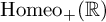 . Therefore,
$\Gamma $
. Therefore,
$\Gamma $
 is also left-orderable. Applying Theorem C, we conclude that
$\Gamma $
is also left-orderable. Applying Theorem C, we conclude that
$\Gamma $
 admits a nontrivial Hilbert transform.
Recall that this gives a new example of a group multiplier satisfying Cotlar’s identity, but not a new example of a group multiplier being
$L_p$
 bounded since it falls within the theory described in [Reference Randrianantoanina74]. In order to obtain new examples outside both the classical theory, the theory of free Hilbert transforms [Reference Mei and Ricard55] and the theory of subdiagonal algebras, we will need an example of a group with property (FA) acting without global fixed points on an
$\mathbb {R}$
bounded since it falls within the theory described in [Reference Randrianantoanina74]. In order to obtain new examples outside both the classical theory, the theory of free Hilbert transforms [Reference Mei and Ricard55] and the theory of subdiagonal algebras, we will need an example of a group with property (FA) acting without global fixed points on an
$\mathbb {R}$
 -tree other than
$\mathbb {R}$
-tree other than
$\mathbb {R}$
 itself. There are a few examples in that direction in the literature; see [Reference Minasyan57], but the complexity of the constructions makes finding explicit formulas for the multipliers more involved.
6 Hilbert transforms over lattices of
$\mathrm {SL}_2(\mathbb {R})$
and
$\mathrm {SL}_2(\mathbb {C})$


The modular group
$\mathrm {PSL}_2(\mathbb {Z})$
 is a discrete subgroup of
$\mathrm {PSL}_2(\mathbb {R})$
is a discrete subgroup of
$\mathrm {PSL}_2(\mathbb {R})$
 . Over
$\mathrm {PSL}_2(\mathbb {R})$
. Over
$\mathrm {PSL}_2(\mathbb {R})$
 there is a very natural multiplier symbol, playing a role analogous to that of the Hilbert transform in
$\mathbb {R}$
there is a very natural multiplier symbol, playing a role analogous to that of the Hilbert transform in
$\mathbb {R}$
 . This is given by equation (1.7). In the statement of the following theorem we will abuse our notation and write the elements in
$\mathrm {PSL}_2(\mathbb {R})$
. This is given by equation (1.7). In the statement of the following theorem we will abuse our notation and write the elements in
$\mathrm {PSL}_2(\mathbb {R})$
 , which are classes of matrices up to a sign, simply by matrices. We will also denote by S and T the matrices

It holds that
$S^2 = -\mathrm {id}$
 and
$(ST)^3=-\mathrm {id}$
and
$(ST)^3=-\mathrm {id}$
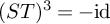 , which in the quotient group gives that
$S^2=\mathrm {id}$
, which in the quotient group gives that
$S^2=\mathrm {id}$
 and
$(ST)^3=\mathrm {id}$
and
$(ST)^3=\mathrm {id}$
 . We have the following result.
Proposition 6.1. Let
$m{|}_{\mathrm {PSL}_2(\mathbb {Z})}: \mathrm {PSL}_2(\mathbb {Z}) \to \mathbb {C}$
 be the restriction of (1.7) to the modular group. Then m satisfies (Cotlar𝔼
⊥) with respect to the subgroup
$\mathrm {G}_0 = \{ \mathrm {id}, S \}$
be the restriction of (1.7) to the modular group. Then m satisfies (Cotlar𝔼
⊥) with respect to the subgroup
$\mathrm {G}_0 = \{ \mathrm {id}, S \}$
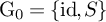 and as a consequence

Proof. First notice that
$m: \mathrm {PSL}_2(\mathbb {R}) \to \mathbb {C}$
 is right K-invariant, with
$K = \mathrm {PSO}(2)$
is right K-invariant, with
$K = \mathrm {PSO}(2)$
 . Similarly, when
$\mathrm {G}_0$
. Similarly, when
$\mathrm {G}_0$
 acts on the left of m we have that

which means that m is left
$\mathrm {G}_0$
 -invariant with respect to a character
$\mathrm {G}_0 \to \mathbb {T}$
-invariant with respect to a character
$\mathrm {G}_0 \to \mathbb {T}$
 and Remark 2.6 applies. We need to prove that
$m(g h) = m(g)$
and Remark 2.6 applies. We need to prove that
$m(g h) = m(g)$
 or
$m(g^{-1}) = m(h)$
or
$m(g^{-1}) = m(h)$
 for
$g \in \mathrm {PSL}_2(\mathbb {Z}) \setminus \mathrm {G}_0$
for
$g \in \mathrm {PSL}_2(\mathbb {Z}) \setminus \mathrm {G}_0$
 and
$h \in \mathrm {PSL}_2(\mathbb {Z}) \setminus \{\mathrm {id}\}$
and
$h \in \mathrm {PSL}_2(\mathbb {Z}) \setminus \{\mathrm {id}\}$
 . Without loss of generality, we can assume that h lives in the larger group
$\mathrm {PSL}_2(\mathbb {R})$
. Without loss of generality, we can assume that h lives in the larger group
$\mathrm {PSL}_2(\mathbb {R})$
 and use the right K-invariance of m to assume that

for some
$x, y \in \mathbb {R}$
 with
$y> 0$
with
$y> 0$
 and
$a, \, b, \, c, \, d \in \mathbb {Z}$
and
$a, \, b, \, c, \, d \in \mathbb {Z}$
 . We are going to use the following elementary identities

If
$m(g^{-1}) = m(h)$
 , then Cotlar’s identity is already fulfilled. Thus, we consider the case when
$m(g^{-1}) \neq m(h)$
, then Cotlar’s identity is already fulfilled. Thus, we consider the case when
$m(g^{-1}) \neq m(h)$
 , which is equal to saying that
$x \, (-ab - dc) < 0$
, which is equal to saying that
$x \, (-ab - dc) < 0$
 . On the other hand, since
$ad - bc = 1$
. On the other hand, since
$ad - bc = 1$
 and
$a, b, c, d \in \mathbb {Z}$
and
$a, b, c, d \in \mathbb {Z}$
 , we get
$abcd = bc + (bc)^2 \geq 0$
, we get
$abcd = bc + (bc)^2 \geq 0$
 . We also get that
$x(ab(d^2 + c^2 ) + dc(a^2 + b^2 )) \geq 0$
. We also get that
$x(ab(d^2 + c^2 ) + dc(a^2 + b^2 )) \geq 0$
 . This observation gives us the following result.

This translates to
$m(gh) = m(g)$
 , which gives the result.
The proposition above also admits a geometric proof. As discussed in the introduction,
$\mathrm {PSL}_2(\mathbb {R})$
 acts faithfully and transitively by isometries on the Poincaré plane
$\mathbb {H}$
acts faithfully and transitively by isometries on the Poincaré plane
$\mathbb {H}$
 via Möbius transformations. As a lattice of
$\mathrm {PSL}_2(\mathbb {R})$
via Möbius transformations. As a lattice of
$\mathrm {PSL}_2(\mathbb {R})$
 ,
$\mathrm {PSL}_2(\mathbb {Z})$
,
$\mathrm {PSL}_2(\mathbb {Z})$
 naturally acts on
$\mathbb {H}$
naturally acts on
$\mathbb {H}$
 . Fix two points
$x_0 = i$
. Fix two points
$x_0 = i$
 and
$x_1 = e^{ \frac {\pi }{3} i} = (1 + \sqrt {-3})/2$
and
$x_1 = e^{ \frac {\pi }{3} i} = (1 + \sqrt {-3})/2$
 on
$\mathbb {H}$
on
$\mathbb {H}$
 , and let y be the geodesic arc joining them. Since
$\mathrm {PSL}_2(\mathbb {Z})$
, and let y be the geodesic arc joining them. Since
$\mathrm {PSL}_2(\mathbb {Z})$
 acts on both arcs and points, we will define X to be the union of all translates of
$g \cdot y$
acts on both arcs and points, we will define X to be the union of all translates of
$g \cdot y$
 for
$g \in \mathrm {PSL}_2(\mathbb {Z})$
for
$g \in \mathrm {PSL}_2(\mathbb {Z})$
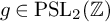 . This union of segments forms a tree, see Figure 10. It is easy to see that the stabilizer of
$x_0$
. This union of segments forms a tree, see Figure 10. It is easy to see that the stabilizer of
$x_0$
 is isomorphic to
$\mathbb {Z}_2$
is isomorphic to
$\mathbb {Z}_2$
 and that of
$x_1$
and that of
$x_1$
 is isomorphic to
$\mathbb {Z}_3$
is isomorphic to
$\mathbb {Z}_3$
 . Indeed, the stabilizer of
$x_0$
. Indeed, the stabilizer of
$x_0$
 is generated by the order
$2$
is generated by the order
$2$
 inversion
$z \mapsto -1/z$
inversion
$z \mapsto -1/z$
 , while the stabilizer of
$x_1$
, while the stabilizer of
$x_1$
 is generated by the order
$3$
is generated by the order
$3$
 map
$z \mapsto (z-1)/z$
map
$z \mapsto (z-1)/z$
 . An elementary computation shows that no nontrivial Möbius transformation with integer coefficients sends
$x_0$
. An elementary computation shows that no nontrivial Möbius transformation with integer coefficients sends
$x_0$
 into
$x_1$
into
$x_1$
 . Therefore, the stabilizer of the edge y is trivial. By the Bass-Serre theory reviewed in Section 5 it is immediate that
$\mathrm {PSL}_2(\mathbb {Z}) \cong \mathbb {Z}_2 \ast \mathbb {Z}_3$
. Therefore, the stabilizer of the edge y is trivial. By the Bass-Serre theory reviewed in Section 5 it is immediate that
$\mathrm {PSL}_2(\mathbb {Z}) \cong \mathbb {Z}_2 \ast \mathbb {Z}_3$
 . Given that
$X \setminus \{x_0\}$
. Given that
$X \setminus \{x_0\}$
 admits two connected components, one lying in the left quadrant and the other in the right, it follows that the multiplier defined in (1.7), when restricted to
$\mathrm {PSL}_2(\mathbb {Z})$
admits two connected components, one lying in the left quadrant and the other in the right, it follows that the multiplier defined in (1.7), when restricted to
$\mathrm {PSL}_2(\mathbb {Z})$
 , fits within Model 1, with the tree given in Figure 10.
Bass-Serre tree of
$\mathrm {PSL}_2(\mathbb {Z})$
 inside the hyperbolic plane.

The case of
$\mathrm {PSL}_2(\mathcal {O}_{-1})$
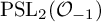 . The purpose of this subsection is to prove Theorem E. Recall that
$\mathrm {PSL}_2(\mathcal {O}_{-1}) \subseteq \mathrm {PSL}_2(\mathbb {C})$
. The purpose of this subsection is to prove Theorem E. Recall that
$\mathrm {PSL}_2(\mathcal {O}_{-1}) \subseteq \mathrm {PSL}_2(\mathbb {C})$
 is a lattice; we will denote such group by
$\Gamma _1$
is a lattice; we will denote such group by
$\Gamma _1$
 . Recall as well that
$\mathrm {PSL}_2(\mathbb {C})$
. Recall as well that
$\mathrm {PSL}_2(\mathbb {C})$
 is semisimple and that any element admits a unique
$KAN$
is semisimple and that any element admits a unique
$KAN$
 -decomposition with
$K =\mathrm {PSU}(2)$
-decomposition with
$K =\mathrm {PSU}(2)$
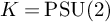 , A the Abelian group of real diagonal matrices and N the nilpotent, in fact Abelian, group of upper triangular complex matrices with ones on the diagonal. More concretely, we have that

Let
$g \in \Gamma _{1}$
 be a matrix of the form

The condition that the determinant equals
$1$
 implies that


Using the two identities above, we can prove elementarily the following key inequality.
Lemma 6.2. Let
$g \in \Gamma _1$
 be as in (6.1). It holds that

Proof. For the first inequality, let
$A = a_1 d_1 + b_2 c_2$
 and
$B = b_1 c_1 + a_2 d_2$
and
$B = b_1 c_1 + a_2 d_2$
 . By equation (6.2) we have
$A = 1 + B$
. By equation (6.2) we have
$A = 1 + B$
 . But this implies that
$A B = B^2 + B$
. But this implies that
$A B = B^2 + B$
 . Since B is an integer
$AB \geq 0$
. Since B is an integer
$AB \geq 0$
 . For the second inequality, it is enough to show that
$0 \leq \mathrm {(I)} - \mathrm {(II)}$
. For the second inequality, it is enough to show that
$0 \leq \mathrm {(I)} - \mathrm {(II)}$
 , where
$\mathrm {(I)} = ( a_1 c_1 + a_2 c_2 ) \, ( b_1 d_1 + b_2 d_2 )$
, where
$\mathrm {(I)} = ( a_1 c_1 + a_2 c_2 ) \, ( b_1 d_1 + b_2 d_2 )$
 and
$\mathrm {(II)} = ( a_1 d_1 + b_2 c_2 ) \, ( b_1 c_1 + a_2 d_2 )$
and
$\mathrm {(II)} = ( a_1 d_1 + b_2 c_2 ) \, ( b_1 c_1 + a_2 d_2 )$
 . We apply (6.3) to obtain

Thus
$\mathrm {(I)} - \mathrm {(II)} = \big ( b_2 c_1 - a_2 d_1 \big ) b_2 c_1 - \big ( b_2 c_1 - a_2 d_1 \big ) a_2 d_2 = (X - Y) X - (X - Y) Y = (X - Y)^2 \geq 0$
 , where
$X = b_2 c_1$
, where
$X = b_2 c_1$
 and
$Y = a_2 d_1$
and
$Y = a_2 d_1$
 .
.
The next lemma follows by elementary calculations.
Lemma 6.3. Let
$g \in \Gamma _{1}$
 as in (6.1).
-
(i) If we assume that $\operatorname {Re} \{a \bar c\} \neq 0$
and
$\operatorname {Re} \{ b\bar d \} \neq 0$
, then we get
$\, \mathrm {sgn} \big ( \operatorname {Re} \{ a\bar c\} \big ) = \mathrm {sgn} \big ( \operatorname {Re} \{ b\bar d \} \big )$
. -
(ii) On the other hand, $\operatorname {Re} \,\{ a\bar c\} \, \operatorname {Re} \, \{ b\bar d\} = 0$
if and only if
$(a_1 d_1 + b_2 c_2)(b_1c_1+a_2d_2)=0$
and
$b_2 c_1 = a_2 d_1$
. -
(iii) If $\operatorname {Re} \{\bar a b\} \neq 0$
and
$\operatorname {Re}\{\bar c d\} \neq 0$
, then
$\mathrm {sgn} (\operatorname {Re} \{\bar a b\})= \mathrm {sgn}( \operatorname {Re} \{\bar c d\} ).$
-
(iv) $\operatorname {Re} \,\{ \bar a b\} \, \operatorname {Re} \, \{\bar c d\} = 0$
if and only if
$\big ( a_1 d_1 + b_2 c_2 \big ) \big ( b_1 c_1 + a_2 d_2 \big ) = 0$
and
$b_1 c_2 = a_2 d_1$
. -
(v) It holds that $\operatorname {Im} \big \{ b \bar c- a \bar d \big \}^2 - 4 \operatorname {Re} \{ a\bar c \} \cdot \operatorname {Re} \{ b\bar d \} \leq 0$
.
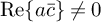
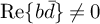




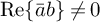
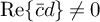





Proof. We will just given an sketch. Observe that, by Lemma 6.2, we have that
$\operatorname {Re}(a\bar {c}) \, \operatorname {Re} (b \bar {d}) \geq 0$
 . Therefore, if both terms are different from zero, they have the same sign. The point (ii) follows similarly by Lemma 6.2 and its proof. Points (iii) and (iv) are a reiteration of the previous two points but changing rows by columns. Lastly, for v, we start by noticing that

where we have used (6.3). Now, we have that


where
$X = a_2 d_2 + b_1 c_1$
 . We have used identity (6.3) in (6.4), and (6.5). For (6.6) we use (6.2). The last term is negative since X is an integer and
$X^2 + X$
. We have used identity (6.3) in (6.4), and (6.5). For (6.6) we use (6.2). The last term is negative since X is an integer and
$X^2 + X$
 is always positive when
$X \in \mathbb {Z}$
is always positive when
$X \in \mathbb {Z}$
 .
.
Now let us consider the symbol given in (1.8). When restricted to
$\Gamma _1$
 , it is
$0$
, it is
$0$
 over a large subset. We are going to show that this subset is in fact a subgroup
$\Gamma _0 \subseteq \Gamma _1$
over a large subset. We are going to show that this subset is in fact a subgroup
$\Gamma _0 \subseteq \Gamma _1$
 . The following proposition follows from the previous lemma.
Lemma 6.4. Let
$g \in \Gamma _{1}$
 be a matrix with coefficients like those in (6.1) and such that
$\operatorname {Re} \{ a \bar c +b \bar d \} = 0$
be a matrix with coefficients like those in (6.1) and such that
$\operatorname {Re} \{ a \bar c +b \bar d \} = 0$
 . Then
$g \in \Gamma _0^+ \cup \Gamma _0^-$
. Then
$g \in \Gamma _0^+ \cup \Gamma _0^-$
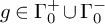 , where

It is clear that
$\Gamma _0^+$
 and
$\Gamma _0 = \Gamma _0^+ \cup \Gamma _0^-$
and
$\Gamma _0 = \Gamma _0^+ \cup \Gamma _0^-$
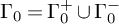 are subgroups of
$\Gamma _1$
are subgroups of
$\Gamma _1$
 with
$[\Gamma _0:\Gamma _0^+] = 2$
with
$[\Gamma _0:\Gamma _0^+] = 2$
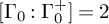 .
.
Proof. Observe that, if
$\operatorname {Re}\{a\bar{c}\}\neq 0$
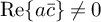 and
$\operatorname {Re}\{b\bar d\}\neq 0$
and
$\operatorname {Re}\{b\bar d\}\neq 0$
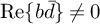 , by Lemma 6.3.(i),
$\operatorname {Re}\{ a \bar{c}\}$
, by Lemma 6.3.(i),
$\operatorname {Re}\{ a \bar{c}\}$
 and
$\operatorname {Re}\{b \bar{d}\}$
and
$\operatorname {Re}\{b \bar{d}\}$
 have the same sign, therefore if
$\operatorname {Re} \{ a \bar{c} + b \bar{d} \} = 0$
have the same sign, therefore if
$\operatorname {Re} \{ a \bar{c} + b \bar{d} \} = 0$
 that is because
$\operatorname {Re} \{a \bar{c}\} = \operatorname {Re} \{b \bar{d}\} = 0$
that is because
$\operatorname {Re} \{a \bar{c}\} = \operatorname {Re} \{b \bar{d}\} = 0$
 . Assume that
$a_1$
. Assume that
$a_1$
 and
$a_2$
and
$a_2$
 are coprime and that
$b_1$
are coprime and that
$b_1$
 and
$b_2$
and
$b_2$
 are also coprime. Since
$\operatorname {Re}\{ a \bar {c}\}= a_1 c_1 + a_2 c_2 = 0$
are also coprime. Since
$\operatorname {Re}\{ a \bar {c}\}= a_1 c_1 + a_2 c_2 = 0$
 , we have that
$(a_1, a_2)$
, we have that
$(a_1, a_2)$
 and
$(c_1, c_2)$
and
$(c_1, c_2)$
 are perpendicular vectors with integer coordinates. But, since
$a_1$
are perpendicular vectors with integer coordinates. But, since
$a_1$
 and
$a_2$
and
$a_2$
 are coprime
$(c_1, c_2) = \ell (a_2, -a_1)$
are coprime
$(c_1, c_2) = \ell (a_2, -a_1)$
 for some
$\ell \in \mathbb {Z}$
for some
$\ell \in \mathbb {Z}$
 . Similarly
$(d_1, d_2) = m \, (b_2, -b_1)$
. Similarly
$(d_1, d_2) = m \, (b_2, -b_1)$
 for some
$m \in \mathbb {Z}$
for some
$m \in \mathbb {Z}$
 . Computing the determinant gives

But this implies that
$m - \ell = \pm 1$
 and
$a_2 b_1 + a_1 b_2 = \pm 1$
and
$a_2 b_1 + a_1 b_2 = \pm 1$
 . Since the imaginary part has to be
$0$
. Since the imaginary part has to be
$0$
 and
$m - \ell = \pm 1$
and
$m - \ell = \pm 1$
 , it follows that
$a_2 b_2 = a_1 b_1$
, it follows that
$a_2 b_2 = a_1 b_1$
 . But since
$a_1$
. But since
$a_1$
 and
$a_2$
and
$a_2$
 , like
$b_1$
, like
$b_1$
 and
$b_2$
and
$b_2$
 , are coprime, we have that
$a_2 = b_1$
, are coprime, we have that
$a_2 = b_1$
 and
$a_1 = b_2$
and
$a_1 = b_2$
 . Therefore
$a_1^2 + a_2^2 = 1$
. Therefore
$a_1^2 + a_2^2 = 1$
 and
$b_1^2 + b_2^2 = 1$
and
$b_1^2 + b_2^2 = 1$
 . Since they are integers, one of
$a_1$
. Since they are integers, one of
$a_1$
 ,
$a_2$
,
$a_2$
 and of
$b_1$
and of
$b_1$
 and
$b_2$
and
$b_2$
 has to be
$0$
has to be
$0$
 . So we have either
$a_2=b_1=0$
. So we have either
$a_2=b_1=0$
 or
$a_1=b_2=0$
or
$a_1=b_2=0$
 . The case of non-coprime
$a_1$
. The case of non-coprime
$a_1$
 and
$a_2$
and
$a_2$
 can be proved similarly, by noticing that
$a_1 + i a_2 = k \alpha _1 + i k \alpha _2$
can be proved similarly, by noticing that
$a_1 + i a_2 = k \alpha _1 + i k \alpha _2$
 with
$k = \gcd (a_1, a_2)$
with
$k = \gcd (a_1, a_2)$
 and
$\alpha _1$
and
$\alpha _1$
 and
$\alpha _2$
and
$\alpha _2$
 coprime. In that case every perpendicular vector to
$(a_1,a_2)$
coprime. In that case every perpendicular vector to
$(a_1,a_2)$
 with integer coordinates is of the form
$(\ell \alpha _2, - \ell \alpha _1)$
with integer coordinates is of the form
$(\ell \alpha _2, - \ell \alpha _1)$
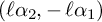 .
.
Observe that
$\Gamma _0^+$
 is isomorphic to the subgroup
$\mathrm {PSL}_2(\mathbb {Z})$
is isomorphic to the subgroup
$\mathrm {PSL}_2(\mathbb {Z})$
 in
$\Gamma _1$
in
$\Gamma _1$
 . Indeed, if we take the natural embedding
$\mathrm {PSL}_2(\mathbb {Z}) \subseteq \Gamma _{1}$
. Indeed, if we take the natural embedding
$\mathrm {PSL}_2(\mathbb {Z}) \subseteq \Gamma _{1}$
 , we have that

The group
$\Gamma _0 = \Gamma _0^+ \cup \Gamma _0^-$
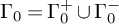 is generated by
$\Gamma _0^+$
is generated by
$\Gamma _0^+$
 and the diagonal matrix with eigenvalues i and
$-i$
and the diagonal matrix with eigenvalues i and
$-i$
 . It is trivial to check that
$\Gamma _0$
. It is trivial to check that
$\Gamma _0$
 is isomorphic to
$\mathrm {PSL}_2(\mathbb {Z}) \rtimes \mathbb {Z}_2$
is isomorphic to
$\mathrm {PSL}_2(\mathbb {Z}) \rtimes \mathbb {Z}_2$
 , with the order two automorphism given by conjugation.
Now, we introduce the following modification of the symbol in (1.8).
Definition 6.5. Let us define the symbol
$m_2: \Gamma _{1} \to \mathbb {C}$
 by
by

Proposition 6.6. The function
$m_2$
 given in Definition 6.5 is both left and right
$\Gamma _0^+$
given in Definition 6.5 is both left and right
$\Gamma _0^+$
 -invariant.
Proof. We first prove that
$m_2$
 is left
$\Gamma _0^+$
is left
$\Gamma _0^+$
 -invariant. Let
$g \in \Gamma _0^{+}$
-invariant. Let
$g \in \Gamma _0^{+}$
 . If
$h \in \Gamma _0^+$
. If
$h \in \Gamma _0^+$
 , since
$\Gamma _0^+$
, since
$\Gamma _0^+$
 is a subgroup of
$\Gamma _1$
is a subgroup of
$\Gamma _1$
 , it is obvious that
$m_2(gh)=m_2(h)=0$
, it is obvious that
$m_2(gh)=m_2(h)=0$
 . If
$h\in \Gamma _0^-$
. If
$h\in \Gamma _0^-$
 , it is easy to check
$gh \in \Gamma _0^-$
, it is easy to check
$gh \in \Gamma _0^-$
 , thus
$m_2(gh)=m_2(h)=1$
, thus
$m_2(gh)=m_2(h)=1$
 . Since
$m_2$
. Since
$m_2$
 , when restricted to
$\Gamma _1 \setminus \Gamma _0$
, when restricted to
$\Gamma _1 \setminus \Gamma _0$
 , is just the hermitian product of its rows, it is clearly right K-invariant. Thus, if
$h\notin \Gamma _0$
, is just the hermitian product of its rows, it is clearly right K-invariant. Thus, if
$h\notin \Gamma _0$
 , we have
$m_2(h)=\operatorname {Re}( t)$
, we have
$m_2(h)=\operatorname {Re}( t)$
 , where

Moreover, we have
$gh \notin \Gamma _0$
 and
and

Now we show
$m_2$
 is right
$\Gamma _0^+$
is right
$\Gamma _0^+$
 -invariant. Similarly to the case above, if
$h \in \Gamma _0^+$
-invariant. Similarly to the case above, if
$h \in \Gamma _0^+$
 ,
$m_2(h g) = m_2(h) = 0$
,
$m_2(h g) = m_2(h) = 0$
 ; if
$h \in \Gamma _0^-$
; if
$h \in \Gamma _0^-$
 , we have
$hg \in \Gamma _0^-$
, we have
$hg \in \Gamma _0^-$
 and
$m_2(hg)=m_2(h)=1$
and
$m_2(hg)=m_2(h)=1$
 . If
$h \notin \Gamma _0$
. If
$h \notin \Gamma _0$
 , let
, let

Then
$h g \notin \Gamma _0$
 . Therefore we have

where

Recall that
$m_2(h)= \mathrm {sgn} \,( {\operatorname {Re} \, (a\bar c +b \bar d}))$
 . If
$\operatorname {Re} \, (a\bar c) \neq 0$
. If
$\operatorname {Re} \, (a\bar c) \neq 0$
 and
$ \operatorname {Re} \, (b\bar d ) \neq 0$
and
$ \operatorname {Re} \, (b\bar d ) \neq 0$
 , then by Lemmas 6.3 and v, it is easy to see
$m_2(hg)=m_2(h)$
, then by Lemmas 6.3 and v, it is easy to see
$m_2(hg)=m_2(h)$
 . If
$\operatorname {Re} \, (a\bar c)=0$
. If
$\operatorname {Re} \, (a\bar c)=0$
 and
$\operatorname {Re} \, (b\bar d)\neq 0$
and
$\operatorname {Re} \, (b\bar d)\neq 0$
 , we have
$m_2(hg)=\mathrm {sgn} [\operatorname {Re}\, (b \bar d) \, u^{-2}]$
, we have
$m_2(hg)=\mathrm {sgn} [\operatorname {Re}\, (b \bar d) \, u^{-2}]$
 and
$m_2(h)=\mathrm {sgn} (\operatorname {Re} \, (b\bar d))$
and
$m_2(h)=\mathrm {sgn} (\operatorname {Re} \, (b\bar d))$
 . Thus
$m_2(hg)=m_2(h)$
. Thus
$m_2(hg)=m_2(h)$
 . If
$\operatorname {Re} \, (a\bar c)\neq 0$
. If
$\operatorname {Re} \, (a\bar c)\neq 0$
 and
$\operatorname {Re} \, (b\bar d)= 0$
and
$\operatorname {Re} \, (b\bar d)= 0$
 , we have
$m_2(hg)=\mathrm {sgn} [ {\operatorname {Re} \, (a\bar c)} \, u^{2} (1+ \, \operatorname {Im}\, v^2)]$
, we have
$m_2(hg)=\mathrm {sgn} [ {\operatorname {Re} \, (a\bar c)} \, u^{2} (1+ \, \operatorname {Im}\, v^2)]$
 and
$m_2(h)=\mathrm {sgn} (\operatorname {Re} \, (a\bar c))$
and
$m_2(h)=\mathrm {sgn} (\operatorname {Re} \, (a\bar c))$
 , which implies
$m_2(hg)=m_2(h)$
, which implies
$m_2(hg)=m_2(h)$
 .
.
Proposition 6.7. The function
$m_2$
 given in Definition 6.5 satisfies the Cotlar identity (Cotlar𝔼
⊥) relative to
$\Gamma _0^+$
given in Definition 6.5 satisfies the Cotlar identity (Cotlar𝔼
⊥) relative to
$\Gamma _0^+$
 , i.e., for any
$g \in \Gamma _{1} \setminus \Gamma _0^+$
, i.e., for any
$g \in \Gamma _{1} \setminus \Gamma _0^+$
 and
$h \in \Gamma _{1}$
and
$h \in \Gamma _{1}$
 , it holds that

Proof. Since
$m_2$
 is right
$\Gamma _0^+$
is right
$\Gamma _0^+$
 -invariant by the Proposition 6.6, it suffices to prove the Cotlar identity for g and h in
$\in \Gamma _1 \setminus \Gamma _0^+$
-invariant by the Proposition 6.6, it suffices to prove the Cotlar identity for g and h in
$\in \Gamma _1 \setminus \Gamma _0^+$
 . That set decomposes as
$\Gamma _1 \setminus \Gamma _0^+ = (\Gamma _1 \setminus \Gamma _0) \sqcup \Gamma _0^-$
. That set decomposes as
$\Gamma _1 \setminus \Gamma _0^+ = (\Gamma _1 \setminus \Gamma _0) \sqcup \Gamma _0^-$
 and thus we have
$4$
and thus we have
$4$
 potential cases. When
$g \in \Gamma _1 \setminus \Gamma _0$
potential cases. When
$g \in \Gamma _1 \setminus \Gamma _0$
 , then for every
$h \in \Gamma _0$
, then for every
$h \in \Gamma _0$
 it holds that
$m_2(gh) = m_2(h)$
it holds that
$m_2(gh) = m_2(h)$
 . In the case in which
$g \in \Gamma _0^-$
. In the case in which
$g \in \Gamma _0^-$
 and
$h \in \Gamma _0^-$
and
$h \in \Gamma _0^-$
 we have that both
$g, h^{-1} \in \Gamma _0^-$
we have that both
$g, h^{-1} \in \Gamma _0^-$
 and as such
$m_2(g) = m_2(h^{-1})$
and as such
$m_2(g) = m_2(h^{-1})$
 . Thus, we can assume that
$g \in \Gamma _1 \setminus \Gamma _0^+$
. Thus, we can assume that
$g \in \Gamma _1 \setminus \Gamma _0^+$
 and
$h \in \Gamma _1 \setminus \Gamma _0$
and
$h \in \Gamma _1 \setminus \Gamma _0$
 . First, let us tackle the case of
$g \in \Gamma _0^-$
. First, let us tackle the case of
$g \in \Gamma _0^-$
 . In this case we have
$m_2(g)=m_2(g^{-1})=1$
. In this case we have
$m_2(g)=m_2(g^{-1})=1$
 . If
$m_2(g^{-1}) = m_2(h)$
. If
$m_2(g^{-1}) = m_2(h)$
 , then the identity is satisfied. If
$m(g^{-1}) \neq m_2(h)$
, then the identity is satisfied. If
$m(g^{-1}) \neq m_2(h)$
 , this implies
$m_2(h)=-1$
, this implies
$m_2(h)=-1$
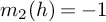 , and then
$h, g h \notin \Gamma _0$
, and then
$h, g h \notin \Gamma _0$
 . By the right K-invariance of
$m_2$
. By the right K-invariance of
$m_2$
 on
$\Gamma _1 \setminus \Gamma _0$
on
$\Gamma _1 \setminus \Gamma _0$
 , we get

Therefore, we get
$m_2(gh)=m_2(g)$
 , so the Cotlar identity is satisfied. Now let us focus on the case of
$g \notin \Gamma _0$
, so the Cotlar identity is satisfied. Now let us focus on the case of
$g \notin \Gamma _0$
 . Let
$g \notin \Gamma _0$
. Let
$g \notin \Gamma _0$
 , i.e.,
$\operatorname {Re} \,(a\bar c +b \bar d)\neq 0$
, i.e.,
$\operatorname {Re} \,(a\bar c +b \bar d)\neq 0$
 and
and

with
$k \in \mathrm {PSU}(2)$
 . We get the following expressions for the four terms appearing in the Cotlar identity:

In the identities for
$m_2(h)$
 and
$m_2(gh)$
and
$m_2(gh)$
 , we have used the property that
$m_2$
, we have used the property that
$m_2$
 is right K-invariant on
$\Gamma _1 \setminus \Gamma _0$
is right K-invariant on
$\Gamma _1 \setminus \Gamma _0$
 . Now we prove the Cotlar identity. If
$m_2(g^{-1}) = m_2(h)$
. Now we prove the Cotlar identity. If
$m_2(g^{-1}) = m_2(h)$
 , then the identity is satisfied. If not, that means

Then we need to show
$m(g) = m(gh)$
 , or in other words,

We first assume that
$\operatorname {Re} \, (a\bar c) \neq 0$
 and
$ \operatorname {Re} \, (b\bar d) \neq 0$
and
$ \operatorname {Re} \, (b\bar d) \neq 0$
 . By Lemma 6.3, we have

Moreover, Lemma 6.3.v implies that the determinant of the quadratic function of
$\operatorname {Im} \,t$
 is negative; together with the inequality above, we see that

Moreover, we claim that

If the claim is true then we will obtain
$m(g) = m(gh)$
 . So now it remains to prove the claim. Notice that by (6.7) and Lemma 6.3, it is enough to show

According to (6.2),
$\operatorname {Re} \, (a\bar d +b \bar c)= a_1 d_1 +a_2 d_2+b_1 c_1 +b_2 c_2 = 2(b_1 c_1 +a_2 d_2)+1$
 . On the other hand, (6.2) and (6.3) imply that

Let
$X= b_1c_1+a_2 d_2$
 ,
$A= a_1^2+a_2^2$
,
$A= a_1^2+a_2^2$
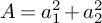 and
$B= a_2^2$
and
$B= a_2^2$
 . Then
$\operatorname {Re}\, (\bar a b) \, \operatorname {Re}\, (a\bar c)\,\operatorname {Re} \, (a\bar d +b \bar c) =(AX+B)(2X+1)$
. Then
$\operatorname {Re}\, (\bar a b) \, \operatorname {Re}\, (a\bar c)\,\operatorname {Re} \, (a\bar d +b \bar c) =(AX+B)(2X+1)$
 . Since
$X\in \mathbb {Z}$
. Since
$X\in \mathbb {Z}$
 and
$|\frac {B}{A}|\leq 1$
and
$|\frac {B}{A}|\leq 1$
 , we get
$(AX+B)(2X+1)\geq 0$
, we get
$(AX+B)(2X+1)\geq 0$
 , which proves the claim.
Now we deal with the case when
$\operatorname {Re} \,( a\bar c) \, \operatorname {Re} \, (b\bar d) = 0$
 . By Lemma 6.3, it is equivalent to saying
$(a_1d_1+b_2c_2)(b_1c_1+a_2d_2)=0 \text { and } b_2c_1=a_2d_1$
. By Lemma 6.3, it is equivalent to saying
$(a_1d_1+b_2c_2)(b_1c_1+a_2d_2)=0 \text { and } b_2c_1=a_2d_1$
 . Without loss of generality, we assume that
$b_1c_1+a_2d_2=0$
. Without loss of generality, we assume that
$b_1c_1+a_2d_2=0$
 . Then by (6.2),
$a_1 d_1 +b_2 c_2=1$
. Then by (6.2),
$a_1 d_1 +b_2 c_2=1$
 . Since
$b_2c_1=a_2d_1$
. Since
$b_2c_1=a_2d_1$
 , (6.3) tells us that
$b_1c_2 = a_1 d_2$
, (6.3) tells us that
$b_1c_2 = a_1 d_2$
 and
$ \operatorname {Im}\,( b\bar c - a\bar d )=2(b_2 c_1 -a_2 d_1)=0$
and
$ \operatorname {Im}\,( b\bar c - a\bar d )=2(b_2 c_1 -a_2 d_1)=0$
 . This implies that

Similarly, we have

Since
$\operatorname {Re} \,( a\bar c+b\bar d)\neq 0$
 ,
$\operatorname {Re} \,( a\bar c)$
,
$\operatorname {Re} \,( a\bar c)$
 and
$ \operatorname {Re} \, (b\bar d) $
and
$ \operatorname {Re} \, (b\bar d) $
 can not be zero at the same time. Suppose
$\operatorname {Re} \,( a\bar c)=0$
can not be zero at the same time. Suppose
$\operatorname {Re} \,( a\bar c)=0$
 and
$ \operatorname {Re} \, (b\bar d ) \neq 0$
and
$ \operatorname {Re} \, (b\bar d ) \neq 0$
 . Then
$m(g)= \mathrm {sgn} \, {\operatorname {Re} \, (b \bar d})$
. Then
$m(g)= \mathrm {sgn} \, {\operatorname {Re} \, (b \bar d})$
 ,
$m(gh) = \mathrm {sgn} \big [ \operatorname {Re} \, (a\bar d +b \bar c)\,\operatorname {Re} \, t + \operatorname {Re}\,( b \bar d) \, s^{-2}\big ]= \mathrm {sgn} \big [ \operatorname {Re} \, t + \operatorname {Re}\, (b \bar d) \, s^{-2}\big ]$
,
$m(gh) = \mathrm {sgn} \big [ \operatorname {Re} \, (a\bar d +b \bar c)\,\operatorname {Re} \, t + \operatorname {Re}\,( b \bar d) \, s^{-2}\big ]= \mathrm {sgn} \big [ \operatorname {Re} \, t + \operatorname {Re}\, (b \bar d) \, s^{-2}\big ]$
 . Applying (6.8) and (6.9), we get
$\operatorname {Re} \, (\bar a b + \bar c d)=(a_1^2 + c_2^2) \operatorname {Re}\, (b \bar d)$
. Applying (6.8) and (6.9), we get
$\operatorname {Re} \, (\bar a b + \bar c d)=(a_1^2 + c_2^2) \operatorname {Re}\, (b \bar d)$
 . Recall that we have
$\operatorname {Re} \, t \cdot \operatorname {Re} \, (\bar a b + \bar c d )>0$
. Recall that we have
$\operatorname {Re} \, t \cdot \operatorname {Re} \, (\bar a b + \bar c d )>0$
 by the assumption
$m(g^{-1})\neq m(h)$
by the assumption
$m(g^{-1})\neq m(h)$
 . Therefore, we have
$\operatorname {Re} \, t \cdot \operatorname {Re}\, (b \bar d)>0$
. Therefore, we have
$\operatorname {Re} \, t \cdot \operatorname {Re}\, (b \bar d)>0$
 , which implies
$m(g)=m(gh)$
, which implies
$m(g)=m(gh)$
 . For the case
$\operatorname {Re} \,( a\bar c)\neq 0$
. For the case
$\operatorname {Re} \,( a\bar c)\neq 0$
 and
$ \operatorname {Re} \, (b\bar d ) = 0$
and
$ \operatorname {Re} \, (b\bar d ) = 0$
 , we omit the proof since it is similar to the previous case.
Now, we can prove Theorem E by just reducing the
$L_p$
 -boundedness of m to that of
$m_2$
-boundedness of m to that of
$m_2$
 .
.
Proof of Theorem E
Notice that
$m: \Gamma _{1} \to \mathbb {C}$
 satisfies that

But Fourier multipliers with symbols being characteristic functions of open subgroups are bounded in
$L_p$
 for every
$1 \leq p \leq \infty $
for every
$1 \leq p \leq \infty $
 . Therefore, up to a finite constant smaller than
$2$
. Therefore, up to a finite constant smaller than
$2$
 , the operator
$L_p$
, the operator
$L_p$
 -norm of
$T_m$
-norm of
$T_m$
 is bounded by that of
$T_{m_2}$
is bounded by that of
$T_{m_2}$
 .
.


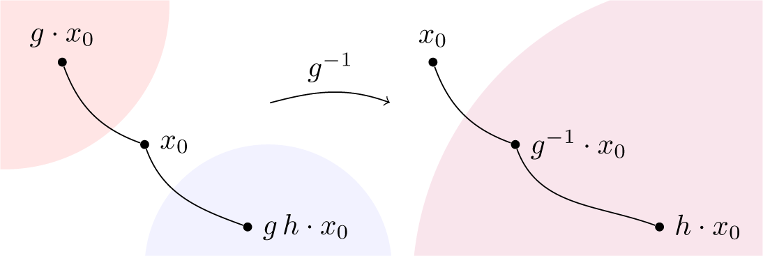
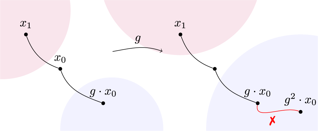

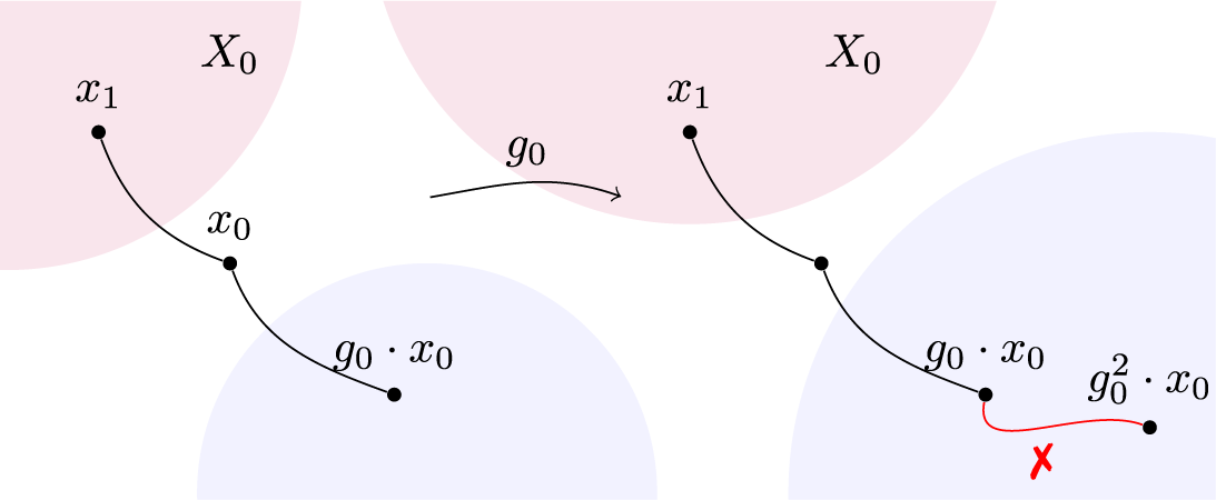


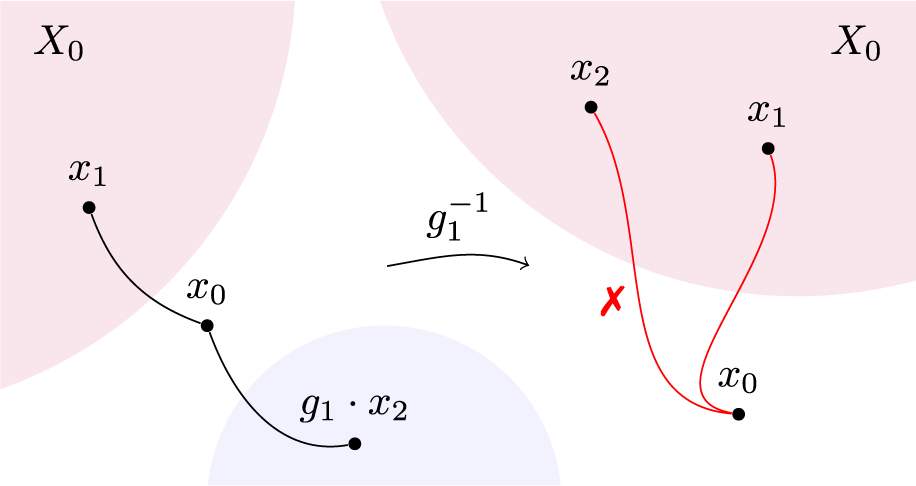


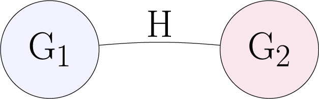
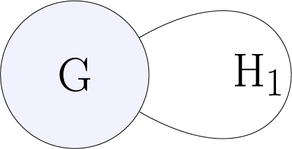
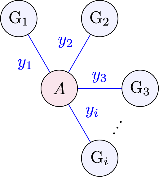
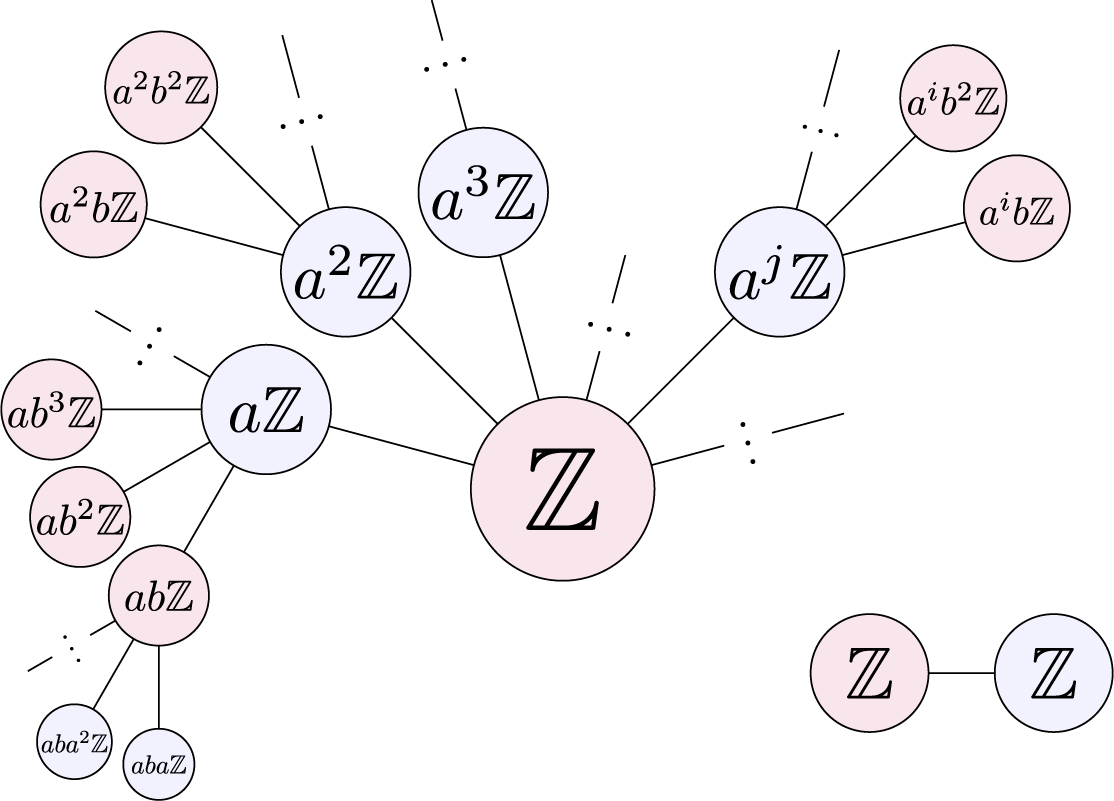


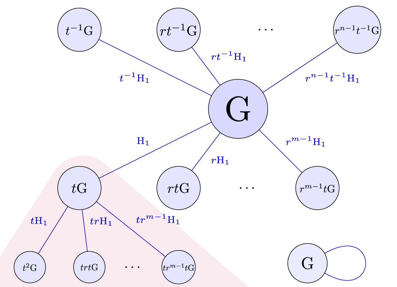


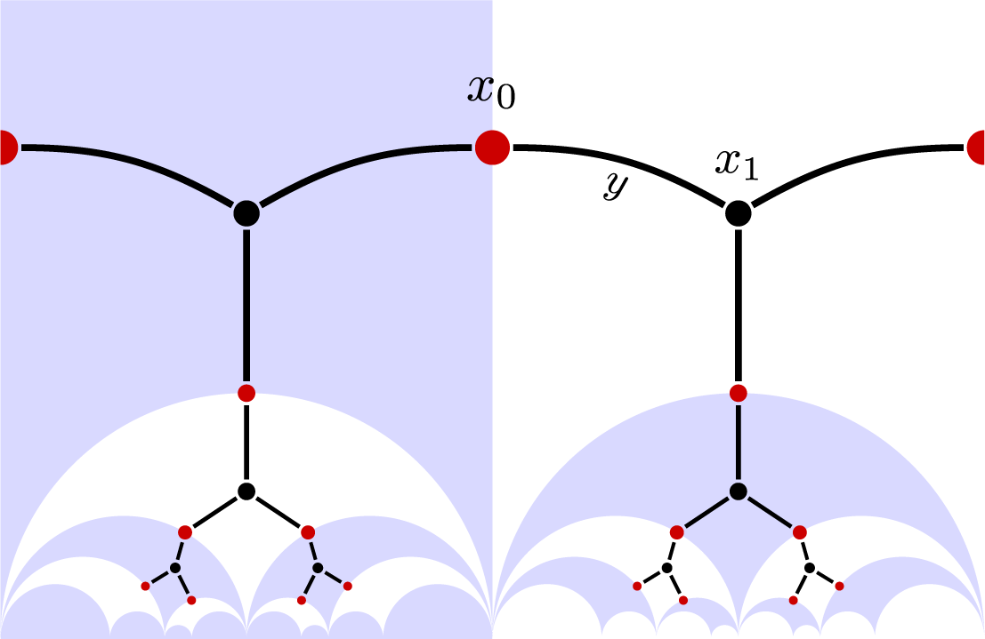


 Open access

