


INTRODUCTION
Numerical modelling of Antarctic ice dynamics becomes more demanding as the simulation time increases, partly because drainage basins evolve and even merge over long timescales, and to a great extent because fine scale features – such as the grounding line – can migrate over continental length scales. Century-long calculations – for example, the simulations of Pine Island Glacier described by Joughin and others (Reference Joughin, Smith and Holland2010), Favier and others (Reference Favier2014), and Seroussi and others (Reference Seroussi2014b) – need only consider single ice streams, and can take advantage of the relatively little grounding line migration that occurs to limit fine resolution to a region close to the present day grounding line. As integration times grow the grounding line tends to sweep out a larger area (Pollard and DeConto, Reference Pollard and DeConto2009) – meaning that the region of fine resolution must either cover that growing area or evolve with it. At the same time, neighbouring ice streams may merge, so that they can no longer be treated separately. Ultimately, it becomes necessary to carry out simulations of the whole of Antarctica, potentially applying fine resolution everywhere.
Adaptive mesh refinement (AMR) methods seek to address the moving grounding line by dynamically generating new non-uniform meshes as the ice sheet evolves. Some effort is needed to ensure that, for example, mass is conserved when the mesh changes, but mature, high performance, general purpose libraries of AMR methods are available to take care of these sorts of issues (Adams and others, Reference Adams2014). Models using AMR have been successful in both idealized tests (Goldberg and others, Reference Goldberg, Holland and Schoof2009; Pattyn and others, Reference Pattyn2013) and in large-scale problems with realistic geometry (Cornford and others, Reference Cornford2015).
MISMIP3d, the Marine Ice Sheet Model Inter-comparison Project for plan view (3-D) models (Pattyn and others, Reference Pattyn2013), was based on an idealized problem that has become something of standard test of ice-sheet models. The problem itself is divided into several parts, but two parts in particular are challenging for ice-sheet models. First, it is necessary to compute a steady state for an ice stream with no lateral variation and a uniform basal traction coefficient. Several of the participating models computed a grounding line many tens of kilometres from the correct position (given their stress approximation), depending on mesh resolution and other aspects of the numerical treatment. Second, a slippy spot is introduced, which results in the center of the ice stream advancing and the edges retreating. After 100 a the slippy spot is removed and eventually the ice sheet should return to its original steady state: some models failed to achieve this reversibility.
Subgrid friction schemes, such as those in Seroussi and others (Reference Seroussi, Morlighem, Larour, Rignot and Khazendar2014a), Leguy and others (Reference Leguy, Asay-Davis and Lipscomb2014), Gladstone and others (Reference Gladstone, Payne and Cornford2010), and Feldmann and others (Reference Feldmann, Albrecht, Khroulev, Pattyn and Levermann2014), improve the performance of vertically integrated, hydrostatic models for a given resolution in the MISMIP3d test. They are simpler than AMR, in two senses: they are easier to implement and they do not add further degrees of freedom to the most computationally expensive parts of the computation, such as solving the stress balance equations. It is not automatically true that these schemes will perform as well in realistic problems, because there are other fine scale features to consider, such as ice stream shear margins. On top of that, realistic problems tend to have lower friction coefficients than in MISMIP3d, at least in fast flowing regions, so the step change in basal traction at the grounding line is smaller. It seems reasonable to anticipate better performance from methods that lack a subgrid friction scheme as the step amplitude decreases, so it is not at all clear that the magnitude of relative improvements seen in MISMIP3d should be expected in general. Given that ~500 m resolution (We will use the symbol ~ to indicate decimal order-of-magnitude, so that Δx ~ a means 10−1/2 a <Δx < 101/2 a and, for example, 0.5, 1 and 2 km are all ~1 km.) is needed without a subgrid friction scheme in at least some realistic cases (Favier and others, Reference Favier2014), the suggestion that an order-of-magnitude coarser resolution might become sufficient simply by introducing such a scheme (Feldmann and others, Reference Feldmann, Albrecht, Khroulev, Pattyn and Levermann2014), needs to be tested.
In this paper we take the obvious step: adding a subgrid friction scheme to the BISICLES AMR ice-sheet model. Rather than carrying out an idealized test, we compare the performance of the resulting method with the original AMR scheme in a 1000 year simulation of the entire Antarctic ice sheet. Our intention is to subject the model to a variety of conditions representing the real problems to be solved, though we are limited in that sense by the need to make at least some assumptions: the choice of basal traction law, the oceanic and atmosphere forcing, and so on. We focus on qualitative and quantitative aspects of numerical error, and show that mesh sensitivity in a realistic problem may be large and vary considerably across physical locations and numerical treatments, but can be quantified in a simple fashion, and so should be quantified routinely.
METHODS
The BISICLES ice-sheet model has been described elsewhere (Cornford and others, Reference Cornford2013), but a few key points are relevant to this paper. A vertically integrated stress balance equation (Schoof and Hindmarsh, Reference Schoof and Hindmarsh2010) is solved to determine the horizontal ice velocity at the lower surface of the ice ${\vec u^{\rm b}}(x,\;y)$
: it is akin to the shallow-shelf approximation but with simplified vertical shear strains included in the effective viscosity. Traction at the base of grounded ice is given by a Weertman (Weertman, Reference Weertman1957) law
${\vec u^{\rm b}}(x,\;y)$
: it is akin to the shallow-shelf approximation but with simplified vertical shear strains included in the effective viscosity. Traction at the base of grounded ice is given by a Weertman (Weertman, Reference Weertman1957) law
 $${\vec \tau ^{\,\rm b}} = - C(x,\;y) \left\vert {\vec u^{\rm b}}(x,\;y) \right\vert ^{1/m - 1}{\vec u^{\rm b}}(x,\;y),$$
with m = 3, which results in a discontinuous stress field across the grounding line. That means that longitudinal stretching increases over a short-length scale, which we resolve by applying ~500 m or finer spatial resolution. Since such fine resolution is only required close to the grounding line, we reduce computational time through a conservative adaptive mesh method, where a block-structured mesh evolves over time to maintain fine resolution where it is needed, while employing coarser resolution elsewhere.
BISICLES' original discretization employs one-sided differences in the region around the grounding line but apart from that makes no special provisions. The integral of the x-component of gravitational driving stress over square cells with side Δx immediately upstream in the x-direction from the grounding line is approximated with a one-sided formula
 $$\eqalign{ & \rho g\int_{{x_{\rm i}} - \Delta x/2}^{{x_{\rm i}} + \Delta x/2} \int_{{y_{\rm i}} - \Delta x/2}^{{y_{\rm i}} + \Delta x/2} h\displaystyle{{\partial s} \over {\partial x}}\;{\rm d}x\;{\rm d}y \cr & \quad \approx \displaystyle{{\rho g} \over 2}({h_{{\rm i} - 1,{\rm j}}} + {h_{{\rm i,j}}})({s_{{\rm i,j}}} - {s_{{\rm i} - 1,{\rm j}}})\Delta x} $$
rather than the more usual central difference, and similar one sided formulae are deployed downstream and in the y-direction. The integral of the basal traction over each cell is approximated with the mid-point rule
 $$\int_{{x_{\rm i}} - \Delta x/2}^{{x_{\rm i}} + \Delta x/2} \int_{{y_{\rm i}} - \Delta x/2}^{{y_{\rm i}} + \Delta x/2} {\vec \tau ^{\,\rm b}}{\rm d}x{\kern 1pt} {\rm d}y \approx - {C_{{\rm i,j}}} \left\vert \vec u_{{\rm i,j}}^{\rm b} \right\vert ^{1/m - 1}\vec u_{{\rm i,j}}^{\rm b} \Delta {x^2}\comma$$
where $\vec \tau _{{\rm i,j}}^{\,\rm b} $
is the value of the basal traction at the cell center. If
$\vec \tau _{{\rm i,j}}^{\,\rm b} $
is the value of the basal traction at the cell center. If ${\vec \tau ^{\,\rm b}}$
were continuous and differentiable this formula would lead to O(Δx
2) truncation error: since it is discontinuous across the grounding line the error is O(Δx). This scheme resulted in errors in the steady-state grounding line positions in the MISMIP3d test of between 10 and 20 times the finest mesh spacing Δx
f, depending on the stress approximation.
${\vec \tau ^{\,\rm b}}$
were continuous and differentiable this formula would lead to O(Δx
2) truncation error: since it is discontinuous across the grounding line the error is O(Δx). This scheme resulted in errors in the steady-state grounding line positions in the MISMIP3d test of between 10 and 20 times the finest mesh spacing Δx
f, depending on the stress approximation.
A comparison can be made between the one-sided difference scheme in Cornford and others (Reference Cornford2013) and the ISSM (Ice Sheet System Model) friction schemes in Seroussi and others (Reference Seroussi, Morlighem, Larour, Rignot and Khazendar2014a). In Cornford and others (Reference Cornford2013), the shallow-shelf approximation model places its MISMIP3d steady grounding line at x = 583 km given Δx = 1.6 km and at x = 595 km given Δx = 0.8 km (and at x = 605 km given Δx = 0.1 km). Seroussi and others (Reference Seroussi, Morlighem, Larour, Rignot and Khazendar2014a) compared two subgrid friction schemes (SEP1 and SEP2, for Sub-Element Parametrization 1 and 2) with an un-modified scheme (NSEP, for No Sub-Element Parametrization). When Δx = 1.0 km ISSM/SEP1 has a steady grounding line at 605 km, ISSM/SEP2 at 592 km, and ISSM/NSEP at 481 km. These are to be compared with an analytic approximation, which places the grounding line at x = 607 km. In other words, the original BISICLES scheme had a similar sized error to ISSM/SEP2, but far lower error than ISSM/NSEP, which we attribute at least in part to the one-sided difference because in preliminary tests – prior to Cornford and others (Reference Cornford2013) – we observed much larger error in the more usual centered-difference scheme.
An alternative scheme along the lines of Feldmann and others (Reference Feldmann, Albrecht, Khroulev, Pattyn and Levermann2014) can be constructed by complementing the one-sided difference with a reduced friction coefficient determined through bi-linear interpolation of the thickness above flotation. Each cell is divided into quadrants and the thickness above flotation h − h
f interpolated between four cell centers; for example, in the upper-right quadrant we interpolate between the values of h − h
f at ${\vec x_{{\rm i,j}}}$
,
${\vec x_{{\rm i,j}}}$
, ${\vec x_{{\rm i} + 1,{\rm j}}}$
,
${\vec x_{{\rm i} + 1,{\rm j}}}$
, ${\vec x_{{\rm i,j} + 1}}$
and
${\vec x_{{\rm i,j} + 1}}$
and ${\vec x_{{\rm i} + 1,{\rm j} + 1}}$
. We then subdivide each quadrant into 2
n
× 2
n
equal parts, and count the subdivisions where h > h
f to estimate the grounded ice fraction of the cell,
${\vec x_{{\rm i} + 1,{\rm j} + 1}}$
. We then subdivide each quadrant into 2
n
× 2
n
equal parts, and count the subdivisions where h > h
f to estimate the grounded ice fraction of the cell, $w_{{\rm i,j}}^n \in [0,\;1]$
, and replace (3) with
$w_{{\rm i,j}}^n \in [0,\;1]$
, and replace (3) with
 $$\int_{{x_{\rm i}} - \Delta x/2}^{{x_{\rm i}} + \Delta x/2} \int_{{y_{\rm i}} - \Delta x/2}^{{y_{\rm i}} + \Delta x/2} {\vec \tau ^{\,\rm b}}{\rm d}x{\kern 1pt} {\rm d}y \approx w_{{\rm i,j}}^n {C_{{\rm i,j}}} \left\vert \vec u_{{\rm i,j}}^{\rm b} \right\vert ^{1/m - 1}\vec u_{{\rm i,j}}^{\rm b} \Delta {x^2}.$$
We will refer to the resulting schemes as SGn, and in particular, study the case n = 4.
The truncation error in (4) is O(Δx). First, expressing (4) only in terms of ${\vec u_{{\rm i,j}}}$
, rather than
${\vec u_{{\rm i,j}}}$
, rather than ${\vec u_{{\rm i,j}}}$
and its neighbours, is second-order accurate only if
${\vec u_{{\rm i,j}}}$
and its neighbours, is second-order accurate only if $\vec \tau _{{\rm i,j}}^{\,\rm b} $
is continuous. Second, the quadrature formula used to evaluate the integral is second-order accurate only if a chain of subdivision faces approximate the grounding line to O(Δx
2). It is certainly possible to achieve this higher-order accuracy, and even straightforward in 1-D, but only worth the effort if the viscous and driving stresses can be treated in the same way. We plan to report on such a scheme, based on the EBChombo embedded boundary and AMR toolkit, in the future.
$\vec \tau _{{\rm i,j}}^{\,\rm b} $
is continuous. Second, the quadrature formula used to evaluate the integral is second-order accurate only if a chain of subdivision faces approximate the grounding line to O(Δx
2). It is certainly possible to achieve this higher-order accuracy, and even straightforward in 1-D, but only worth the effort if the viscous and driving stresses can be treated in the same way. We plan to report on such a scheme, based on the EBChombo embedded boundary and AMR toolkit, in the future.
We tested our numerical methods by carrying out ka simulations of the entire Antarctic continent. Sensitivity to mesh resolution is examined by repeating the same experiment for both the SG0 and SG4 schemes with five different mesh spacings. The coarsest mesh is a simple uniform grid of Δx
0 = 8 km squares. Progressively finer meshes are built from rectangular regions of finer cells, with Δx
ℓ = 2−ℓ × 8 km, where ℓ ∈ ℕ and 0 < ℓ < L, and choosing a maximum value 0 < L ≤ 4. In other words, experiments SG0/Δx
L
and SG4/Δx
L
have cells with mesh spacing as fine as Δx
L
and as coarse as 8 km. Meshes are generated every few time steps, starting from a uniform 8 km mesh and refining according to two criteria. Fine resolution is maintained around the grounding line by covering at least the distance 8Δx
ℓ either side with Δx
ℓ cells. Since the bedrock DEM has kilometer-scale features, we also refine the mesh along the ice streams by imposing $\left\vert\vec u\right\vert\Delta {x^\ell} \lt 3.0 \times {10^5}\;{{\rm m}^2}\;{{\rm a}^{ - 1}}$
if Δx
ℓ ≥ 1 km.
$\left\vert\vec u\right\vert\Delta {x^\ell} \lt 3.0 \times {10^5}\;{{\rm m}^2}\;{{\rm a}^{ - 1}}$
if Δx
ℓ ≥ 1 km.
Starting from an initial state close to the present day, the model is subjected to an extreme oceanic melt rate, varying linearly from no melt at all where the ice shelf is 100 m thick or less, to 800 m a−1 where it is more than 400 m thick. Total ablation across all the ice shelves is ~ 104 − 105 km3 a−1 in the early stages of the experiments, compared with estimates ~ 103 km3 a−1 for the present day (Depoorter and others, Reference Depoorter2013; Rignot and others, Reference Rignot, Jacobs, Mouginot and Scheuchl2013). This is clearly not at all realistic: we are simply attempting to study the numerical properties of the model as the grounding line migrates over a significant region. It certainly does so. Figure 1 shows the ice sheet at the start and end of one of the more finely resolved simulations. By the end of the simulation, most of the marine sections of West Antarctica are afloat, and there is also considerable retreat in some sections of East Antarctica. At the same time the mesh has evolved with the grounding line and has swept across most of West Antarctica.
Flow speed (left) and mesh spacing (right) at the start of (top) and 600 a into (bottom) the SG4/0.5 km experiment, painted onto the ice surface. The grounding line sweeps over most of West Antarctica, and there is also substantial retreat in several parts of East Antarctica, including the Bailey, Slessor and Recovery Glaciers, the Sabrina Coast including Totten Glacier, and George V Land in the region of the Wilkes Subglacial Basin. The computational mesh evolves with the ice sheet, maintaining fine resolution (~0.5 km) close to the grounding line and in regions of fast flow, but treating the majority of the domain at coarser (8 km) resolution.

Note that the oceanic melt rate is strictly zero in any cell whose center is grounded, as the alternative, namely interpolation of the melt rate in a similar fashion to the basal traction, is vulnerable to an unphysical mechanism. Melting of the first cell upstream from the grounding line would be averaged across the whole cell, thinning it until it becomes ice shelf, which would thin further until the interpolated grounding line entered the next cell upstream, and so on. The result is grounding line retreat driven entirely by numerical error (Durand and Pattyn, Reference Durand and Pattyn2015). That is exactly the mechanism responsible for the physically impossible retreat that occurs when an unbuttressed ice shelf with no lateral variation is thinned in Feldmann and Levermann (Reference Feldmann and Levermann2015) and would also seem to be responsible for the retreat in George V Land computed with the same methods – see Golledge and others (Reference Golledge2015) where such retreat is conditional on the use of a subgrid melt scheme. In contrast, George V Land retreat in this paper is due to ice dynamics, and only occurs at 1 km or finer resolution when the subgrid friction scheme is in play, and 0.5 km when it is not.
The initial state in each case is derived from the same maps of bedrock elevation, initial thickness, basal traction coefficient C(x, y) and a stiffening coefficient ϕ(x, y), which relates to the ice viscosity. C(x, y) and ϕ(x, y) are determined in the usual way (see Cornford and others (Reference Cornford2015) for details), solving an inverse problem to match model speed with observed speed (Rignot and others, Reference Rignot, Mouginot and Scheuchl2011). The bedrock elevation and initial thickness are derived from bedmap2 (Fretwell and others, Reference Fretwell2013), but the bedrock is modified (as in Nias and others (Reference Nias, Cornford and Paynein press)) to avoid a thickening tendency in Pine Island Glacier (Rignot and others, Reference Rignot, Mouginot, Morlighem, Seroussi and Scheuchl2014), which also results in an initial grounding line in that region close to its 2007 configuration. Surface mass balance (Arthern and others, Reference Arthern, Winebrenner and Vaughan2006) and temperature (Pattyn, Reference Pattyn2010) fields are held constant-in-time. Each of these fields is averaged or interpolated onto the various meshes as required.
RESULTS
Broadly speaking, the most coarsely resolved simulations exhibit far less grounding line retreat or loss of grounded ice than the most finely resolved simulations. To convince ourselves that the mesh is fine enough in any given case SGn/Δx L km, we need to demonstrate two simple properties. First, the coarser resolution solutions must comprise a Cauchy (and hence convergent) sequence, that is, the solutions found for SGn/Δx L km and SGn/2Δx L km are closer together than SGn/2Δx L km and SGn/4Δx L km. Second, the difference between the SGn/Δx L km and SGn/2Δx L km results, which is a natural estimate of the error in the SGn/Δx L km model given that the scheme is first order, should be sufficiently small. The second property is meaningless without the first, and the meaning of ‘sufficiently small’ depends on the application, so we will primarily examine convergence of the grounding line position and of the change in volume above flotation.
Change in volume above flotation
Figure 2 plots the change ΔV f and rate of change dV f/dt of volume above flotation for each simulation. ΔV f is perhaps the most important summary statistic in an ice dynamic simulation, as it can be converted directly into eustatic sea-level rise, and we will report it here in meters sea level equivalent (m s.l.e). It is immediately clear that although switching to the SG4 subgrid friction scheme always results in a faster rate of loss and more overall loss, there is comparable mesh sensitivity in both cases, and larger variation due to resolution than choice of friction scheme. Both Δx L = 0.5 km experiments result in ~4 m s.l.e mass lost over ka (4.4 m s.l.e for SG4/0.5 km and 3.8 m s.l.e for SG0/0.5 km), while both Δx L = 8 km experiments exhibit far less (0.9 m s.l.e for SG4/8 km and −0.5 m s.l.e for SG0/8 km).
Change in volume above flotation (ΔV f, top), and rate of change (dV f/dt, bottom) over time. |ΔV f| grows as the finest mesh spacing Δx min shrinks in both SG0 (squares, left) and SG4 (discs, right) simulations, with − ΔV f varying from − 0.5 to 4.4 m s.l.e. The difference between pairs of curves ΔV f(Δx L ) and ΔV f(Δx L /2) begins to decay once Δx L ≤ 2 km in the SG4 case and Δx L ≤ 1 km in the SG0 case. A 200 a long period of elevated volume loss is visible in all but the coarsest resolution experiments, and starts earlier in finer resolution experiments.

Convergence is, however, superior in SG4. In both cases, the ΔV f are closer together at finer resolutions, but in the SG4 case convergence begins at a coarser resolution. Once Δx ≤ 2 km, the mean difference between successive pairs of curves ΔV f(Δx L ) − ΔV f(2Δx L ) begins to decay at a first-order rate, roughly halving if the mesh spacing is halved. From that, we estimate the error in the total mass loss in SG4/0.5 km to be 0.3 m s.l.e and in SG4/1.0 km to be 0.7 m s.l.e. A similar pattern of first-order convergence does not set in until Δx L ≤ 1 km for SG0, and in that case we estimate the error in the SG4/0.5 km total mass loss to be 0.8 m s.l.e. Put simply, SG4/1.0 km has a marginally smaller error than SG0/0.5 km, and SG4/0.5 km has an appreciably smaller error.
As the mesh is refined, both the SG0 and SG4 models exhibit a particular feature in ΔV f(t) and its time derivative. Mass loss decelerates from a maximum at the start of the experiment, but undergoes a roughly two-century period of acceleration. The onset of this acceleration varies from t = 1000 in the SG0/2 km experiment and t = 400 a in the SG4/2 km experiment to t = 250 a in the SG4/1 km experiment, at which point it is hard to distinguish. The acceleration itself is associated with the final major phase of West Antarctic Ice Sheet (WAIS) collapse when the Amundsen Sea Embayment (ASE) and Siple Coast ice streams merge. As with the total loss of volume above flotation, the onset of the final phase converges with mesh refinement, provided Δx L ≤ 2 km in the SG0 case and Δx L ≤ 4 km in the SG4 case.
If we consider ΔV f(t) alone, the SG4 scheme has a lower error than the SG0 scheme given the same mesh parameters. All of the SG4/Δx L curves lie between the SG0/Δx L /2 and SG0/Δx L /4 curves, so that switching from the SG0 scheme to the SG4 scheme improves performance more than adding one level of refinement, but less than adding two.
Grounding line retreat
Figure 3 shows each experiment's grounding line after 300, 600 and 900 a in the regions that see significant grounding line retreat: West Antarctica and Coats Land, the Sabrina Coast and the coast of George V Land. Overall there is a great deal of variation in mesh sensitivity between ice streams, which determines when, if ever, WAIS enters the final phase of collapse. In particular, the grounding line retreats over hundreds of kilometers in the Siple Coast and in the west and south of the Filchner-Ronne Ice Shelf in every experiment but retreats slowly, if at all, in the ASE unless Δx ≤ 2 km. Thwaites Glacier is an extreme example, becoming a primary contributor to WAIS collapse only when Δx ≤ 1 km. We will return to Thwaites Glacier after detailing the retreat elsewhere.
WAIS, Sabrina coast and George V Land grounding lines and ∂h/∂t plotted at 300, 600 and 900 a for the SG0 (left column) and SG4 (right column) simulations. Grounding lines are shown for every simulation, while ∂h/∂t is shown for the two Δx L = 0.5 km simulations.

Many of the ice streams flowing into the west and south of the Filchner-Ronne Ice Shelf retreat even given the coarsest meshes. The Möller and Institute ice stream grounding lines retreat across the Robin Subglacial Basin in the first 300 a of every experiment, albeit more slowly and stabilizing sooner at coarser resolutions, with the Bungenstock Ice Rise disappearing in every case but the SG0/8 km. Foundation Ice Stream behaves similarly, although the neighbouring Support Force Glacier sees its retreat attenuated prematurely in all but the SG0/0.5 km, SG4/1.0 km and SG4/0.5 km calculations. Evans Ice Stream and Rutford Ice Stream also retreat in every case, although the extent of their retreat is restricted to their present day fast flow when Δx = 8 km. Given finer resolutions, their basins merge with that of Carson inlet and the combined ice stream diverts the upper reaches of Pine Island Glacier's catchment into the Filchner-Ronne Ice Shelf.
Grounding line retreat also occurs at all resolutions in the Siple Coast. Results are qualitatively similar in all of the SG4 experiments, with significant grounding line retreat in every ice stream but Kamb Ice Stream, the northern portion of which is left as an isolated ice rise by the end of the simulations. The same is true for SG0 once Δx ≤ 2 km. Nonetheless, quantitative sensitivity to the mesh refinement is evident, with slower retreat at coarser resolutions, particularly in the SG0 cases.
If Pine Island Glacier retreats at all, it does so quickly enough for its grounding line to merge with Evans and Rutford ice streams within 300 a. Just as in earlier simulations (Cornford and others, Reference Cornford2013; Favier and others, Reference Favier2014; Cornford and others, Reference Cornford2015), the grounding line tends not to retreat at all in coarser resolution simulations without the subgrid friction scheme (SG0/8 km, SG0/4 km), and even at moderate resolution (SG0/2 km) retreat along the majority of the trunk does not occur within the first 300 a. With the subgrid friction scheme, only the coarsest resolution experiment (SG4/8 km) shows no retreat at all, although major retreat is delayed until after 300 a in the SG4/4 km experiment.
Crossing from West to East Antarctica, Slessor Glacier's grounding line retreats hundreds of kilometers within the first 300 a of each simulation and Bailey Ice Stream behaves similarly in all but the SG0/8 km experiment. In contrast, the nearby Recovery Glacier sees its grounding line stabilize on a ridge ~50 km upstream of its present day position in all but the SG4/1 km and SG4/0.5 km, where it crosses the ridge to a second stable position more than 200 km further upstream. Support Force Glacier also exhibits far more retreat in the finest resolution (SG0/0.5 km, SG4/1 km, SG4/0.5 km) experiments.
Grounding line retreat in the bulk of East Antarctica is rather less extensive but just as variable with respect to resolution requirements. The Sabrina Coast ice streams including Totten Glacier retreat readily with all but the coarsest meshes, before their conjoined grounding lines find a stable position on slopes rising to the south, forming an ice shelf that separates the continent proper from Law Dome. The opposite is true of the ice streams flowing into the Cook Ice Shelf in George V Land. They barely retreat at all unless mesh resolution is 1 km or finer, in which case the grounding line retreats by ~200 km to form a circular ice shelf with a narrow throat.
A number of ice streams exhibit episodic retreat, in particular those that require the finest resolution. As well as grounding line retreat, Figure 4 shows the instantaneous ice thickness tendency ∂h/∂t for the two Δx L = 0.5 km experiments. Recovery Glacier, for example, is thinning at a rate of <1 m a−1 300 a into both the SG0 and SG4 simulations, with its grounding line positioned on top of the first ridge described earlier. If thinning was sustained at that rate more than 1000 years would elapse before the grounding line retreated to the second ridge (since (h − h f)/(∂h/∂t) >1 ka between the two ridges) but in both the SG4/1 km and SG0/0.5 km calculations, thinning accelerates once the first ridge is crossed, so that the grounding line reaches the second ridge in <300 a. Similar episodes of retreat can be seen in Pine Island Glacier, Support Force Glacier and elsewhere, but the most obvious and important example is Thwaites Glacier, whose grounding line retreats at a rate of <0.5 km a−1 over the 1st century, while crossing a region of shallow bedrock incised by a deep channel but then accelerates to more than 1.5 km a−1 into a rapidly deepening and widening trough. An analogous acceleration was noted in Joughin and others (Reference Joughin, Smith and Medley2014).
Resolution dependence in Thwaites Glacier. The colour-map shows ice flow speed, while the black contour indicates the grounding line and the blue contour depicts the initial grounding line for comparison. Under-resolved calculations – with Δx L ≥ 2 km for SG4 and Δx L ≥ 1 km for SG0 – see Thwaites Glacier retreat slowly, so that its flow is diverted through a glacier that arises in Byrd Trench and flows out through an ice shelf occupying the former catchments of Pine Island Glacier, Evans Ice Stream and Rutford Ice Stream. In finer resolution calculations – with Δx L ≤ 1 km for SG4 and Δx L ≤ 0.5 km for SG0 – Thwaites Glacier retreats far more quickly, shedding its mass through the present day flux gate into the Amundsen Sea until it joins with the Siple Coast glaciers through the Bentley Trench.
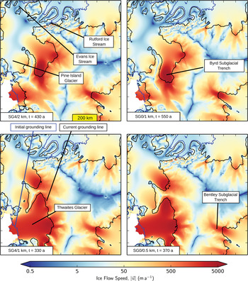
Mesh sensitivity in Thwaites Glacier
Although SG4 models with Δx L ≤ 2.0 km and SG0 models with Δx L ≤ 1.0 km all enter the final phase of WAIS collapse before the end of the experiment, the timing and mechanism of that event indicates that finer resolution is required. Figure 4 shows the flow speed and grounding line in a region around Thwaites Glacier and the Bentley Subglacial Trench shortly before the ice divide between them is breached in experiments SG0/1 km, SG0/0.5 km, SG4/2 km and SG4/1 km. At coarser resolution, the final phase of collapse takes place beginning ~400–500 a and is initiated by the earlier retreat in Pine Island Glacier, Evans Ice Stream and Rutford Ice Stream. At finer resolution it begins a century sooner and is initiated by retreat in Thwaites Glacier.
Thwaites Glacier's grounding line retreats by ~100 km over 400–500 a in the SG0/1 km and SG4/2 km experiments. By that time, a new ice stream has formed in the Byrd Subglacial Trench, flowing in an easterly direction through the merged upstream parts of Pine Island Glacier and Rutford Ice Stream's former catchments. The grounding line of that ice stream retreats more quickly than the Thwaites Glacier grounding line, so that the bulk of Thwaites Glacier is diverted and flows across into the ice shelf connecting Pine Island Bay with the Filchner-Ronne Ice Shelf. Ultimately, it is this new ice stream that breaches the major WAIS ice divide, merging with the much-retreated Siple Coast through the Bentley Subglacial Trench. In contrast, in the SG0/0.5 km, SG4/1 km and SG4/0.5 km experiments, Thwaites Glacier retreats quickly enough to breach the ice divide before the new ice stream has diverted its catchment.
DISCUSSION
Perhaps the strongest indication of a need for kilometer or finer mesh resolution and the value of the subgrid friction interpolation is the severe resolution sensitivity in Thwaites Glacier. On one hand the SG4/2 km and SG0/1 km calculations do at least enter the final phase of WAIS collapse within the first 500 a, so that the difference between these and finer resolution simulations might seem small in the context of ka or longer runs. On the other hand that result is likely to depend on substantial ablation of the Filchner-Ronne and Ross ice shelves, something that might be delayed or absent in a realistic ocean model. It remains to be seen whether any version of the model will see WAIS collapse caused only by ocean warming in the ASE, but the far slower retreat of Thwaites Glacier in the SG4/2 km and the SG0/1 km simulations versus the SG4/1 km and SG4/0.5 km would, presumably, see such an event delayed by centuries if it took place at all. And even though the SG0/0.5 km experiment does have the final phase of WAIS collapse caused by retreat in Thwaites Glacier, a yet finer resolution variant – a notional SG0/0.25 km – would be needed to improve on SG4/1 km.
Since there is significant variation in mesh sensitivity between ice streams, there is a real danger that under resolution can lead to qualitatively incorrect conclusions, subgrid schemes notwithstanding. For example, had we accepted the results of the SG4/4 km or SG4/2 km experiments, we might conclude that the ASE ice streams are less sensitive to ocean forcing than the Siple Coast ice streams or the ice streams feeding the south and west of the Filchner-Ronne Ice Shelf. That might not be an unexpected conclusion: if nothing else the large ice shelves surely provide more buttressing than the smaller ones. But finer resolution simulations show that such a conclusion would not be correct.
The results in this paper do not support a general prescription for mesh resolution but instead show that a simple convergence experiment is a practical means to study the potentially large numerical errors that can occur. The difference in mesh sensitivity between the ASE and the Möller and Institute ice streams is a case in point: a study focused on the former region would seem to need 1 km or finer resolution, while a study focused on the latter region might only need 4 km resolution. Looking beyond the results here, Leguy and others (Reference Leguy, Asay-Davis and Lipscomb2014) studied modifications to the usual Weertman basal traction law along the lines of Schoof (Reference Schoof2005) and Gagliardini and others (Reference Gagliardini, Cohen, Råback and Zwinger2007) in the MISMIP3d problem. The laws in question result in basal traction fields that deviate from the Weertman law by decaying to zero over a narrow band upstream from the grounding line. A similar decay occurs in the Coulomb-limited rule proposed by Tsai and others (Reference Tsai, Stewart and Thompson2015), although the underlying physical model differs. Leguy and others (Reference Leguy, Asay-Davis and Lipscomb2014) found that the Weertman rule required a finer resolution for a given accuracy without a subgrid friction scheme, although similar resolution was adequate for either friction law with a subgrid friction scheme. It seems clear to us that the onus is on modellers to show that they have resolved their simulations satisfactorily, and that they cannot rely on extrapolation from idealized problems or realistic problems in different regions or with different physics to decide that.
The need for kilometer or finer mesh resolution even with the subgrid friction scheme means that a uniform mesh would be far more costly than an adaptive mesh, and even a spatially non-uniform but fixed-in-time mesh would carry a premium. The SG4/1 km experiment involved ~5 × 10⁶ floating point numbers for each component of the velocity, some of which are redundant as degrees of freedom but undergo the same operations – see Cornford and others (Reference Cornford2013) for details. A uniform 1 km mesh would require 38 × 106 degrees of freedom to cover the same area with 1 km cells. It is harder to estimate the requirements for a fixed non-uniform mesh, which would depend on the refinement criterion, but since the region that we resolve to 4 km encompasses the majority of the grounding line migration, covering that with 1 km cells to give 10 × 106 degrees-of-freedom might be a reasonable estimate. If finer resolutions are required, the balance tips further: the SG4/0.5 km experiment stored 10 × 106 floating point numbers, while a uniform mesh would store 150 × 106, and a non-uniform mesh perhaps 40 × 106. Overall, every time the mesh spacing is halved, the AMR storage cost doubles, while the fixed mesh cost quadruples. Using an AMR scheme does of course result in additional calculations on top of that implied by additional storage: in our scheme it is dominated by corrections to the velocity needed after the mesh is regenerated and represents at worst a doubling of CPU time, when the mesh is renewed after every time step (Cornford and others, Reference Cornford2013).
Although mesh sensitivity is a major component of ice-sheet model inaccuracy, our experiments hint at least one other, this time related to observations. The grounding line tends to stabilize on a number of ridges where the bedmap2 bedrock is not derived from airborne radar (Fretwell and others, Reference Fretwell2013), sometimes preventing retreat over extensive deep trenches. Denman Glacier's bedrock is derived from a single flightline between the coast and the Aurora subglacial basin: its grounding line comes to rest on a pro-grade slope close to the coast in that sparsely sampled region. Similarly, while there is dense radar coverage of the Wilkes subglacial basin and at the coast, grounding line retreat slows in a ~100 000 km2 area ~200 km inland that lacks any radar data. Recovery Glacier is also well surveyed near to its present day grounding line, but once again retreat is halted on a ridge located in a region of sparse flightline coverage 200 km upstream. Models of East Antarctica's millennium-scale dynamics will remain inaccurate, perhaps on a grand scale, until they include bedrock derived from ice penetrating radar surveys in these three regions.
CONCLUSIONS
Modifying the BISICLES ice-sheet model's treatment of basal traction to include subgrid interpolation of the grounding line improves its truncation error by a factor of two to four in century to millennium scale simulations of the entire Antarctic ice sheet. The impact on computational complexity is considerable, since it allows the use of meshes at least twice as coarse, much as in Gladstone and others (Reference Gladstone, Payne and Cornford2010), but incremental, as kilometer or half-kilometer resolution is needed (rather than half- or quarter-kilometer). Calculations at coarser than 1 km not only underestimate the quantitative rate of retreat, but lead to large-scale qualitative errors as well, particularly in the ASE, and especially in Thwaites Glacier. Although the AMR scheme becomes less efficient relative to fixed mesh methods than it was at finer resolutions, it still reduces the number of degrees of freedom and the overall computational expense by an order of magnitude (rather than two) compared with a uniform mesh method given the required kilometer or finer resolution at the grounding line. Overall, since numerical error in ice dynamics simulations can be large and mesh sensitivity varies with physics and with location, ice flow modelling experiments should be routinely supported by relevant convergence studies.
ACKNOWLEDGEMENTS
Work at the University of Bristol was supported by the NERC CPOM, iSTAR and iGlass consortium projects. Work at Lawrence Berkeley National Laboratory was supported by the Scientific Discovery through Advanced Computing (SciDAC) project funded by the US Department of Energy, Office of Science, Advanced Scientific Computing Research and Biological and Environmental Research under Contract No. DE-AC02-05CH11231. Simulations were carried out using the computational facilities of the Advanced Computing Research Centre, University of Bristol, and resources of the National Energy Research Scientific Computing Center, a DOE Office of Science User Facility supported by the Office of Science of the US Department of Energy under Contract No. DE-AC02-05CH11231. We thank the editor, Jo Jacka, and two anonymous referees for their contributions to this paper.


 Open access