





1. Introduction
Particle–wall interactions in fluid flow occur in many practical settings and are of particular interest at moderate to high Reynolds numbers. Examples include debris removal (Godone & Stanchi Reference Godone and Stanchi2011), ski and aircraft take-off (Virmavirta, Kivekas & Komi Reference Virmavirta, Kivekas and Komi2001), leaf blowing and saltation (Owen Reference Owen1964; Shao, Raupach & Findlater Reference Shao, Raupach and Findlater1993; Foucaut & Stanislas Reference Foucaut and Stanislas1997), food sorting, sand motion and aircraft icing (Gent, Dart & Cansdale Reference Gent, Dart and Cansdale2000; Purvis & Smith Reference Purvis and Smith2016; Norde Reference Norde2017). Theoretical and experimental studies for moving particles of fixed shape in fluid flow at medium to high Reynolds numbers include those by Coulson and Richardson (2019) and Will et al. (Reference Will, Mathai, Huisman, Lohse, Sun and Krug2021). Further theoretical analyses of fixed-shape particles in such flows include Smith (Reference Smith2017) and Palmer & Smith (Reference Palmer and Smith2020), while flexible particles have been considered by Pei, Zhang & Zhou (Reference Pei, Zhang and Zhou2018) and Dotto, Soldate & Marchioli (Reference Dotto, Soldate and Marchioli2019). Of more relevance are applications where phase change accompanies the fluid motion, as in aircraft, marine and engine icing. In these systems, a particle or wall patch may act as a local site of melting or solidification, driven by heat transfer between the solid and fluid phases (Gent et al. Reference Gent, Dart and Cansdale2000; Norde Reference Norde2017). Application to another area, namely the flow of liquid metals containing particles or impurities, is of special interest here.
The main body of this paper seeks to investigate the coupled motion of an inviscid fluid and a freely moving rigid particle which is in flight close to a substrate which can melt or solidify. The substrate is embedded within a solid wall, and can either accrete material that creates a hump or melt away and create a cavity. The particle is nearly aligned with the surrounding wall which is taken to be locally flat. The substrate and surrounding fluid are composed of the same material and are taken to have nearly equal densities. The particle, being hotter or colder than the ambient fluid, serves as a finite heat source or sink, inducing melting or solidification of the nearby substrate. The fluid flow couples with the particle motion via the pressure forces acting on the particle surface. In addition, however, the consequent alteration in the shape of the fluid-filled gap between the wall and the particle surface enhances or decreases the thermal transfer effect, showing that the phase change is dependent on the fluid flow, as well as vice versa. This work seeks to investigate how the particle geometry and the substrate–particle temperature difference influence the particle trajectory and the evolution of the substrate boundary position.
The model described above for a rigid particle and phase-changing substrate can be readily adapted to the case of a rigid substrate and a phase-changing particle. This scenario is discussed in Appendix A, and shows that heating or cooling of the fixed substrate induces particle melting or fluid solidification, respectively. The particle thus changes shape, thereby altering the fluid dynamics and the heat transfer as well as the particle motion. This particular application is of industrial interest due to the possible potential improvements in efficiency achieved by suitably adjusting or intermittently turning off the substrate heating, enough to prevent particles impacting on the wall.
In this work, we consider a regime in which the Reynolds number based on the particle length is large and the Prandtl number is small. The characteristic time scales associated with substrate phase change and fluid motion are assumed to be comparable, so that unsteady effects due to particle melting/solidification and the hydrodynamics are fully coupled. The densities of the fluid and solid phases are taken to be comparable (as is physically relevant when both phases consist of the same material) and, for simplicity, are hence assumed equal throughout the analysis. The above assumptions are most consistent with metallic systems (Zwirner & Shishkina Reference Zwirner and Shishkina2018; Kalantar-Zadeh, Rahim & Tang Reference Kalantar-Zadeh, Rahim and Tang2021; Kim et al. Reference Kim, Schindler, Vogt and Eckert2024; Krishnamurthi et al. Reference Krishnamurthi2024), as will be shown later in § 2, where representative parameter values are presented. In particular, they correspond to situations in which a liquid metal flows over a substrate and a boundary layer forms, see Bian & Rangel (Reference Bian and Rangel1996) and Lofgren (Reference Lofgren2001) for example, and background studies by Katgerman (Reference Katgerman1988), Kurz & Fisher (Reference Kurz and Fisher1992), Carpenter & Steen (Reference Carpenter and Steen1997), Steen & Karcher (Reference Steen and Karcher1997), Löfgren & Åkerstedt (Reference Löfgren and Åkerstedt1998) and Nyström et al. (Reference Nyström, Reichelt and Dubke2003). In this setting, the particle is interpreted as a solid impurity within the liquid metal, and for tractability the particle thickness is comparable to the width of the fluid gap between the particle and wall (Wilson & Smith Reference Wilson and Smith2011; Jolley & Smith Reference Jolley and Smith2024). The fluid is assumed inviscid and incompressible and the flow to be laminar and unsteady in two dimensions.
Concerning comparisons with existing recent theoretical studies, the current modelling is similar to that in Jolley & Smith (Reference Jolley and Smith2024) in the sense that the density ratio is $\mathcal{O}(1)$
, but incorporation of phase-change effects is a major novel feature here. Other analytical works on fluid/particle interactions for large Reynolds numbers (Wilson & Smith Reference Wilson and Smith2011; Palmer & Smith Reference Palmer and Smith2020; Liu, Yazar & Smith Reference Liu, Yazar and Smith2023) are usually valid only for large density ratios and in many cases take the flow to be quasi-steady, unlike in the present work.
$\mathcal{O}(1)$
, but incorporation of phase-change effects is a major novel feature here. Other analytical works on fluid/particle interactions for large Reynolds numbers (Wilson & Smith Reference Wilson and Smith2011; Palmer & Smith Reference Palmer and Smith2020; Liu, Yazar & Smith Reference Liu, Yazar and Smith2023) are usually valid only for large density ratios and in many cases take the flow to be quasi-steady, unlike in the present work.
The remainder of the paper is constructed as follows. In § 2, the governing equations are presented and the reduced model is formulated. In § 3, we then present and discuss numerical solutions of the model which illustrate four types of terminal behaviour: a collision (strictly near collision) between the substrate boundary and front, middle or back of the particle, or a fly-away phenomenon as the particle departs comparatively far from the substrate. The asymptotic structure of solutions in the case of a mid-body collision is presented in § 4. Conclusions and discussions follow in § 5.
2. Governing equations
Our main concern is with the scenario of a thin rigid in-flow particle positioned above a wall-embedded substrate whose boundary can evolve due to phase change. A schematic of the model geometry is provided in figure 1. The interaction considered involves melting or accretion of the substrate due to the comparatively hot or cold particle. The resulting change in the fluid gap between the particle and substrate alters the hydrodynamic forces on the particle, which in turn feeds back on the fluid temperature and the substrate melting rate. This three-way interaction between fluid flow, particle motion and phase change is nonlinear in general. The underlying equations are the continuity and Navier–Stokes equations for the fluid motion, those of rigid-particle motion for the particle and a thermal equation for the fluid temperature. These are coupled with a Stefan condition which determines the position of the substrate. The particle is modelled as thin, lying close to (and almost aligned with) a straight fixed wall and moving in the presence of an incident uniform stream of fluid with streamwise velocity $U^*$
. The asterisk denotes a dimensional quantity.
$U^*$
. The asterisk denotes a dimensional quantity.
The fluid in question is composed of the same material as the substrate. Consequently, the fluid and solid densities are comparable, and in the present work we take them to be identical, denoted by $\rho ^*$
. The characteristic gap width
$\rho ^*$
. The characteristic gap width $W^*$
between the substrate and the particle underbody is small compared with the particle length
$W^*$
between the substrate and the particle underbody is small compared with the particle length $L^*$
in the streamwise direction (Smith & Ellis Reference Smith and Ellis2010; Wilson & Smith Reference Wilson and Smith2011; Jolley & Smith Reference Jolley and Smith2024). We work with dimensionless distances, velocities, times and pressures which are scaled with
$L^*$
in the streamwise direction (Smith & Ellis Reference Smith and Ellis2010; Wilson & Smith Reference Wilson and Smith2011; Jolley & Smith Reference Jolley and Smith2024). We work with dimensionless distances, velocities, times and pressures which are scaled with $L^*,\,U^*,\,L^*/U^*$
and
$L^*,\,U^*,\,L^*/U^*$
and $\rho U^{*2}$
, respectively, together with the ratio
$\rho U^{*2}$
, respectively, together with the ratio $W^*/L^*:=\varepsilon \ll 1$
being small. The time scales of the fluid flow and the phase change are assumed comparable. The fluid is taken to be not only incompressible but also inviscid in effect, which is justified provided
$W^*/L^*:=\varepsilon \ll 1$
being small. The time scales of the fluid flow and the phase change are assumed comparable. The fluid is taken to be not only incompressible but also inviscid in effect, which is justified provided $\varepsilon$
is large compared with the typical boundary layer thickness, which is of order
$\varepsilon$
is large compared with the typical boundary layer thickness, which is of order $\textit{Re}^{-1/2}$
where the Reynolds number
$\textit{Re}^{-1/2}$
where the Reynolds number $\textit{Re}$
is based on the particle length. The overall interaction is modelled as two-dimensional in the
$\textit{Re}$
is based on the particle length. The overall interaction is modelled as two-dimensional in the $L^*(x,\,\varepsilon y)$
plane, where
$L^*(x,\,\varepsilon y)$
plane, where $x$
and
$x$
and $y$
describe the dimensionless longitudinal and lateral position. The corresponding unknown fluid velocity and pressure are
$y$
describe the dimensionless longitudinal and lateral position. The corresponding unknown fluid velocity and pressure are $U^*(u,\,\varepsilon v)$
and
$U^*(u,\,\varepsilon v)$
and $\rho ^* U^{*2}p$
, where
$\rho ^* U^{*2}p$
, where $u,\,v$
denote the longitudinal and lateral dimensionless velocity components and
$u,\,v$
denote the longitudinal and lateral dimensionless velocity components and $p$
the dimensionless pressure. The particle occupies the interval
$p$
the dimensionless pressure. The particle occupies the interval $0\lt x\lt 1$
and its angles of inclination during its motion are assumed to be of order
$0\lt x\lt 1$
and its angles of inclination during its motion are assumed to be of order $\varepsilon ,$
the same as those of the fluid-filled gap. As in Jolley & Smith (Reference Jolley and Smith2024), the particle overbody shape can also be specified, however, provided it remains thin it does not contribute to the leading-order interaction as the corresponding induced pressure variation is small compared with that of the underbody.
$\varepsilon ,$
the same as those of the fluid-filled gap. As in Jolley & Smith (Reference Jolley and Smith2024), the particle overbody shape can also be specified, however, provided it remains thin it does not contribute to the leading-order interaction as the corresponding induced pressure variation is small compared with that of the underbody.
A schematic illustrating the dimensionless model geometry, where $H(x,\,t)$
denotes the gap width and
$H(x,\,t)$
denotes the gap width and $y=F(x,\,t),\,G_s(x,\,t)$
describe the position of rigid-particle underbody and substrate boundary.
$y=F(x,\,t),\,G_s(x,\,t)$
describe the position of rigid-particle underbody and substrate boundary.

As discussed in § 1, the assumptions outlined in the introduction and the preceding paragraph are consistent with liquid-metal flows, and parameter value estimates are now discussed to justify this. Typical material properties for molten metals are a dynamic viscosity of order $\mu ^* \approx 10^{-3}\,\mathrm{Pa\,s}$
and a density of
$\mu ^* \approx 10^{-3}\,\mathrm{Pa\,s}$
and a density of $\rho ^* \approx 5 \times 10^3\,\mathrm{kg\,m^{-3}}$
(Dinsdale & Quested Reference Dinsdale and Quested2004). We take the characteristic velocity scale to be
$\rho ^* \approx 5 \times 10^3\,\mathrm{kg\,m^{-3}}$
(Dinsdale & Quested Reference Dinsdale and Quested2004). We take the characteristic velocity scale to be $U^* \approx 10^{-1}\,\mathrm{m\,s^{-1}},$
consistent with reported molten steel flow velocities in industrial casting processes (Zhang, Yang & Jiang Reference Zhang, Yang and Jiang2019); see also Lofgren (Reference Lofgren2001). Taking the characteristic particle length (interpreted here as an impurity within the flowing metal) to be
$U^* \approx 10^{-1}\,\mathrm{m\,s^{-1}},$
consistent with reported molten steel flow velocities in industrial casting processes (Zhang, Yang & Jiang Reference Zhang, Yang and Jiang2019); see also Lofgren (Reference Lofgren2001). Taking the characteristic particle length (interpreted here as an impurity within the flowing metal) to be $L^* \approx 10^{-2}\,\mathrm{m}$
, the corresponding Reynolds number
$L^* \approx 10^{-2}\,\mathrm{m}$
, the corresponding Reynolds number $\textit{Re} = \rho ^* U^* L^* / \mu$
is
$\textit{Re} = \rho ^* U^* L^* / \mu$
is $\textit{Re} \approx 5 \times 10^3$
, which justifies the large
$\textit{Re} \approx 5 \times 10^3$
, which justifies the large $\textit{Re}$
assumption taken in this work. As noted above, viscous effects are negligible provided
$\textit{Re}$
assumption taken in this work. As noted above, viscous effects are negligible provided $\textit{Re}^{-1/2} \ll \varepsilon$
. For the representative values of
$\textit{Re}^{-1/2} \ll \varepsilon$
. For the representative values of $L^*$
and
$L^*$
and $\textit{Re}$
above, this condition suggests that the present analysis can apply when
$\textit{Re}$
above, this condition suggests that the present analysis can apply when $W^* \approx 1.4 \times 10^{-3}\,\mathrm{m}$
, corresponding to
$W^* \approx 1.4 \times 10^{-3}\,\mathrm{m}$
, corresponding to $\varepsilon \approx 1.4 \times 10^{-1}$
. For liquid-metal flows, the Prandtl number is typically small. Using values for the kinematic viscosity which is calculated from
$\varepsilon \approx 1.4 \times 10^{-1}$
. For liquid-metal flows, the Prandtl number is typically small. Using values for the kinematic viscosity which is calculated from $\mu$
and
$\mu$
and $\rho ^*$
above alongside a thermal diffusivity of
$\rho ^*$
above alongside a thermal diffusivity of $\alpha ^* \approx 2 \times 10^{-5}\, \mathrm{m}^2\, \mathrm{s}^{-1}$
(Stankus, Savchenko & Agazhanov Reference Stankus, Savchenko and Agazhanov2012) gives the Prandtl number
$\alpha ^* \approx 2 \times 10^{-5}\, \mathrm{m}^2\, \mathrm{s}^{-1}$
(Stankus, Savchenko & Agazhanov Reference Stankus, Savchenko and Agazhanov2012) gives the Prandtl number $\sigma = \mu ^*/(\rho ^*\alpha ^*)$
as
$\sigma = \mu ^*/(\rho ^*\alpha ^*)$
as $\sigma \approx 10^{-2},$
thus suggesting the small
$\sigma \approx 10^{-2},$
thus suggesting the small $\sigma$
limit exploited subsequently. Using the above values, the characteristic flow time scale,
$\sigma$
limit exploited subsequently. Using the above values, the characteristic flow time scale, $L^*/U^*$
, is approximately
$L^*/U^*$
, is approximately $0.1\,\mathrm{s}$
. On the other hand, the phase-change time scale,
$0.1\,\mathrm{s}$
. On the other hand, the phase-change time scale, $W^{*2}/(\alpha ^* \textit{St})$
, where
$W^{*2}/(\alpha ^* \textit{St})$
, where $\textit{St} = c_p \Delta T / L_{\kern-1pt f}$
is the Stefan number (with
$\textit{St} = c_p \Delta T / L_{\kern-1pt f}$
is the Stefan number (with $c_p$
,
$c_p$
, $\Delta T$
and
$\Delta T$
and $L_{\kern-1pt f}$
denoting the specific heat, temperature variation and latent heat, respectively), is also
$L_{\kern-1pt f}$
denoting the specific heat, temperature variation and latent heat, respectively), is also $0.1\,\mathrm{s}$
provided that
$0.1\,\mathrm{s}$
provided that $\textit{St} \approx 1$
. This justifies the assumption that the solidification and flow time scales are comparable.
$\textit{St} \approx 1$
. This justifies the assumption that the solidification and flow time scales are comparable.
The equations governing the fluid flow, given the above assumptions on particle and fluid slenderness, and the absence of any incident vorticity (since the incident flow has $u = 1$
and
$u = 1$
and $v = 0$
), reduce to the thin-layer form
$v = 0$
), reduce to the thin-layer form
 \begin{align} \frac {\partial H}{\partial t}+\frac {\partial }{\partial x}(uH) &=0, \\[-12pt] \nonumber \end{align}
 \begin{align} \frac {\partial u}{\partial t}+u\frac {\partial u}{\partial x}&=-\frac {\partial p}{\partial x}, \\[10pt] \nonumber \end{align}
where $H$
is the scaled unknown gap width between the substrate boundary and particle underbody. The corresponding scaled gap pressure
$H$
is the scaled unknown gap width between the substrate boundary and particle underbody. The corresponding scaled gap pressure $p$
is of order unity and satisfies the Bernoulli constraint at the particle leading edge where
$p$
is of order unity and satisfies the Bernoulli constraint at the particle leading edge where $x=0$
and the Kutta condition at the trailing edge where
$x=0$
and the Kutta condition at the trailing edge where $x=1$
, so that
$x=1$
, so that
 \begin{align} p&=\frac {1}{2} \big(1-u^2 \big) \quad \,\text{at} \quad x=0, \\[-12pt] \nonumber \end{align}
 \begin{align} p&=0 \quad \qquad \quad \,\,\,\,\, \text{at} \quad x=1.\\[10pt] \nonumber \end{align}
We note there are thin viscous layers present on the particle surfaces which are assumed separation free. Concerning the Kutta condition from (2.2b
), we note in addition that, and in contrast with the $\mathcal{O}(1)$
pressures in the gap, the pressure contributions above the particle are negligible to leading order
$\mathcal{O}(1)$
pressures in the gap, the pressure contributions above the particle are negligible to leading order $\varepsilon$
, in view of the fluid flow slenderness and the
$\varepsilon$
, in view of the fluid flow slenderness and the $\mathcal{O}(\varepsilon )$
particle slopes. We now consider the remaining two components of the interaction, namely the particle motion and substrate phase change.
$\mathcal{O}(\varepsilon )$
particle slopes. We now consider the remaining two components of the interaction, namely the particle motion and substrate phase change.
Denoting the position of the unknown substrate boundary and particle underbody as $y=G_s(x,\,t)$
and
$y=G_s(x,\,t)$
and $y=F(x,\,t)$
, respectively, the fluid-filled gap width is then given by
$y=F(x,\,t)$
, respectively, the fluid-filled gap width is then given by $H=F-G_s.$
As discussed above, the particle overbody motion does not contribute to the leading-order interaction and is hence neglected here. The case of
$H=F-G_s.$
As discussed above, the particle overbody motion does not contribute to the leading-order interaction and is hence neglected here. The case of $G_s\lt 0$
corresponds to scenario where the substrate boundary has melted beneath the wall at
$G_s\lt 0$
corresponds to scenario where the substrate boundary has melted beneath the wall at $y=0$
, whereas
$y=0$
, whereas $G_s\gt 0$
represents ice accretion in the form of a hump. We suppose that
$G_s\gt 0$
represents ice accretion in the form of a hump. We suppose that $F = F_p(x)+h(t)+(x-\beta )\theta (t)$
such that
$F = F_p(x)+h(t)+(x-\beta )\theta (t)$
such that $F_p$
is the given shape of the particle underbody, whereas
$F_p$
is the given shape of the particle underbody, whereas $h(t)$
and
$h(t)$
and $\theta (t)$
describe the unknown lateral and rotational particle position, respectively. Here,
$\theta (t)$
describe the unknown lateral and rotational particle position, respectively. Here, $x=\beta$
denotes the prescribed position of the particle centre of mass. To clarify, the function
$x=\beta$
denotes the prescribed position of the particle centre of mass. To clarify, the function $h(t)$
represents the scaled time dependence of the
$h(t)$
represents the scaled time dependence of the $y$
-coordinate of the centre of mass, which is fixed within the particle. Its horizontal motion is negligible to leading order in
$y$
-coordinate of the centre of mass, which is fixed within the particle. Its horizontal motion is negligible to leading order in $\varepsilon .$
In view of the above relations, we have that
$\varepsilon .$
In view of the above relations, we have that
 \begin{align} H =G(x,\,t)+h_c(t)+x\theta (t), \end{align}
where $G= F_p(x)-G_s(x,\,t)$
and
$G= F_p(x)-G_s(x,\,t)$
and $h_c=h-\beta \theta .$
It is assumed that the particle underbody shape and the evolving substrate boundary shape are relatively smooth and their slopes are not too extreme. Otherwise flow separation may occur in the thin viscous boundary layers on the underbody and on the substrate, either locally to, say, a discontinuity in slope or globally: the latter global separation would require re-modelling of the flow.
$h_c=h-\beta \theta .$
It is assumed that the particle underbody shape and the evolving substrate boundary shape are relatively smooth and their slopes are not too extreme. Otherwise flow separation may occur in the thin viscous boundary layers on the underbody and on the substrate, either locally to, say, a discontinuity in slope or globally: the latter global separation would require re-modelling of the flow.
The equations governing the motion of the rigid particle, and hence evolution of $h(t)$
and
$h(t)$
and $\theta (t)$
require a balance between mass-acceleration effects and fluid-pressure forces. In the present situation of a near-wall slender particle of density comparable to that of the surrounding fluid, a scaling argument indicates that forces induced by the fluid pressure dominate the mass-acceleration terms. Hence, particle motion is governed by (Jolley & Smith Reference Jolley and Smith2024)
$\theta (t)$
require a balance between mass-acceleration effects and fluid-pressure forces. In the present situation of a near-wall slender particle of density comparable to that of the surrounding fluid, a scaling argument indicates that forces induced by the fluid pressure dominate the mass-acceleration terms. Hence, particle motion is governed by (Jolley & Smith Reference Jolley and Smith2024)
 \begin{align} \int _0^1 p\, \mathrm{d}x=\int _0^1 xp\, \mathrm{d}x = 0, \end{align}
corresponding to a configuration where the so-called added mass is dominant over the actual particle mass. We note that the argument of the second integral here is strictly $(x-\beta ),$
although the first integral is used to reduce it to its current form.
$(x-\beta ),$
although the first integral is used to reduce it to its current form.
The particle and substrate are assumed to have uniform density, with the substrate boundary temperature taken as the melt temperature, which is normalised to zero. The dimensional fluid temperature is written as $T^*= T^*_m+(T^*_w-T^*_m)T,$
where
$T^*= T^*_m+(T^*_w-T^*_m)T,$
where $T^*_m$
and
$T^*_m$
and $T^*_w$
denote the characteristic dimensional melting and particle temperature, respectively. The dimensionless fluid temperature
$T^*_w$
denote the characteristic dimensional melting and particle temperature, respectively. The dimensionless fluid temperature $T(x,\,y,\,t)$
is governed by the thermal transport equation
$T(x,\,y,\,t)$
is governed by the thermal transport equation
 \begin{align} \frac {\partial T}{\partial t}+u\frac {\partial T}{\partial x} {+v\frac {\partial T}{\partial y}} = {\frac {1}{\varepsilon ^2\textit{Re}\,\sigma }\frac {\partial ^2 T}{\partial y^2}, } \end{align}
where $\sigma$
is the Prandtl number. Dissipation effects are neglected here as in Moore, Mughal & Papageorgiou (Reference Moore, Mughal and Papageorgiou2017), Jepson, Batley & Smith (Reference Jepson, Batley and Smith2025) and Batley & Smith (Reference Batley and Smith2025), on account of the representative thermal range associated with
$\sigma$
is the Prandtl number. Dissipation effects are neglected here as in Moore, Mughal & Papageorgiou (Reference Moore, Mughal and Papageorgiou2017), Jepson, Batley & Smith (Reference Jepson, Batley and Smith2025) and Batley & Smith (Reference Batley and Smith2025), on account of the representative thermal range associated with $\theta$
dominating over the speed range proportional to
$\theta$
dominating over the speed range proportional to $u^2$
. We assume that the particle underbody temperature is prescribed as
$u^2$
. We assume that the particle underbody temperature is prescribed as $T_p(x,\,t)$
, where
$T_p(x,\,t)$
, where $T_p\gt 0$
or
$T_p\gt 0$
or $T_p\lt 0$
is expected to relate to melting or solidification of the wall-mounted substrate. Recalling that the substrate boundary temperature is zero, the boundary conditions on
$T_p\lt 0$
is expected to relate to melting or solidification of the wall-mounted substrate. Recalling that the substrate boundary temperature is zero, the boundary conditions on $T$
are thus
$T$
are thus
 \begin{align} T&=0 \qquad \,\,\,\text{at} \quad y=G_s, \\[-12pt] \nonumber \end{align}
 \begin{align} T&=T_p \qquad \text{at} \quad y=F. \\[10pt] \nonumber \end{align}
The temperature beneath the substrate is assumed to be zero in this paper, which points to the heat flux within the substrate being negligible. The position of the melting or solidifying substrate, to leading order in $\varepsilon ,$
is then governed by the Stefan condition
$\varepsilon ,$
is then governed by the Stefan condition
 \begin{align} \frac {\partial G_s}{\partial t} = -b\frac {\partial T}{\partial y} \qquad \text{at} \quad y=G_s, \end{align}
where the constant $b\gt 0$
is directly proportional to the Stefan number.
$b\gt 0$
is directly proportional to the Stefan number.
In view of the parameter values discussed above, we now take the small Prandtl number limit $\sigma \ll \varepsilon ^{-2}\textit{Re}^{-1},$
so that the left-hand side of (2.5) is negligible, leaving the right-hand side equating zero. The thermal response is thus distinct from the flow response in the sense that the convection effects alone are not significant in the gap (unlike the inertial contributions in the fluid flow). Using the boundary conditions from (2.6), we hence obtain to leading order
$\sigma \ll \varepsilon ^{-2}\textit{Re}^{-1},$
so that the left-hand side of (2.5) is negligible, leaving the right-hand side equating zero. The thermal response is thus distinct from the flow response in the sense that the convection effects alone are not significant in the gap (unlike the inertial contributions in the fluid flow). Using the boundary conditions from (2.6), we hence obtain to leading order
 \begin{align} T = \frac {T_p}{H}(y-G_s), \end{align}
so that the Stefan condition from (2.7) provides
 \begin{align} \frac {\partial G_s}{\partial t} = -b\frac {T_p}{H}, \end{align}
which relates the evolution of the substrate shape directly to the local wall temperature and the local gap width.
The coupling of the fluid flow, particle motion and fluid temperature is captured by the system (2.1)–(2.4) and (2.9). These equations are subject to initial conditions on the substrate $G_s$
and the mass flux entering the gap at
$G_s$
and the mass flux entering the gap at $x=0,$
as well as on
$x=0,$
as well as on $h,\, \theta$
and their first derivatives. The necessity and application of these conditions is seen more clearly in the following section. In general the system described above is nonlinear and must be solved numerically, as described in the next section. It is found subsequently that the computational results point to further analysis and insight.
$h,\, \theta$
and their first derivatives. The necessity and application of these conditions is seen more clearly in the following section. In general the system described above is nonlinear and must be solved numerically, as described in the next section. It is found subsequently that the computational results point to further analysis and insight.
3. Numerical results
In this section, the numerical solutions of the interactive system from (2.1)–(2.4) and (2.9) are discussed, paying particular attention to exemplar parameter values whereby solutions indicate a trailing-edge, leading-edge and mid-body impact between the particle and substrate, and a particle fly-away response. Before this, we discuss the numerical methods used to solve the interactive system.
3.1. Numerical methods
By integrating (2.1a
) in $x$
we obtain
$x$
we obtain
 \begin{align} u = -\frac {1}{H}\bigg [ \int _0^x \frac {\partial H}{\partial t}\, \mathrm{d}\xi +A(t) \bigg ], \end{align}
such that $-A(t)$
denotes the scaled mass flux entering the gap for any
$-A(t)$
denotes the scaled mass flux entering the gap for any $t$
at
$t$
at $x=0.$
Now, integrating (2.1b
) over
$x=0.$
Now, integrating (2.1b
) over $x$
and imposing (2.2) provides
$x$
and imposing (2.2) provides
 \begin{align} \int _0^1 \frac {\partial u}{\partial t} \, \mathrm{d}x = L(t), \end{align}
where $L(t) = {1}/{2} (1-u^2(1,\,t) )$
. Similarly, by multiplying (2.1b
) by
$L(t) = {1}/{2} (1-u^2(1,\,t) )$
. Similarly, by multiplying (2.1b
) by $x$
and then
$x$
and then $x^2$
, integrating over
$x^2$
, integrating over $x$
and then using the lift and moment equations from (2.4), we obtain
$x$
and then using the lift and moment equations from (2.4), we obtain
 \begin{align} \int _0^1 x \frac {\partial u}{\partial t} \, \mathrm{d}x & = \frac {1}{2}\int _0^1 u^2\, \mathrm{d}x-\frac {1}{2}+L(t), \\[-12pt] \nonumber \end{align}
 \begin{align} \int _0^1 x^2 \frac {\partial u}{\partial t} \, \mathrm{d}x & = \int _0^1 xu^2\, \mathrm{d}x-\frac {1}{2}+L(t). \\[10pt] \nonumber \end{align}
The pressure is obtained explicitly in terms of $u$
by integrating (2.1b
) in
$u$
by integrating (2.1b
) in $x$
and using (2.2a
), so that
$x$
and using (2.2a
), so that
 \begin{align} p = -\int _0^x \frac {\partial u}{\partial t}\, \mathrm{d}\xi -\frac {u^2}{2}+\frac {1}{2}. \end{align}
The contributions of $u$
and its first derivative in
$u$
and its first derivative in $t$
seen in the integral system above from (3.2) are obtained by differentiating (3.1) with respect to
$t$
seen in the integral system above from (3.2) are obtained by differentiating (3.1) with respect to $t$
and then substituting
$t$
and then substituting $H$
from (2.3). Denoting
$H$
from (2.3). Denoting $'\equiv ({\partial }/{\partial t})$
for clarity, we have
$'\equiv ({\partial }/{\partial t})$
for clarity, we have
 \begin{align} u& = -\frac {x^2\omega +2(I+vx+A)}{2H}, \\[-12pt] \nonumber \end{align}
 \begin{align} \frac {\partial u}{\partial t}& = \frac {H'\big (x^2\omega +2(I+vx+A) \big )}{2H^2}-\frac {x^2\omega ' +2(J+v'x+A') }{2H} , \\[10pt] \nonumber \end{align}
where $v=h_c'$
and
$v=h_c'$
and $\omega =\theta ',$
and
$\omega =\theta ',$
and
 \begin{align} I(x,\,t) & = b \int _0^x \frac {T_p}{H}\, \mathrm{d}\xi , \\[-12pt] \nonumber \end{align}
 \begin{align} J(x,\,t) & = b \int _0^x \frac {T_p'H-H'T_p}{H^2}\, \mathrm{d}\xi . \\[10pt] \nonumber \end{align}
We note that $H' = bT_p/H+v+x\omega ,$
in view of (2.3) and (2.9).
$H' = bT_p/H+v+x\omega ,$
in view of (2.3) and (2.9).
Using the relations from (3.4), the integral equations from (3.2) are arranged into a system of three nonlinear ordinary differential equations in $t$
, explicitly for
$t$
, explicitly for $v'(t),\,\omega '(t)$
and
$v'(t),\,\omega '(t)$
and $A'(t).$
This couples the equations
$A'(t).$
This couples the equations $h_c'(t)=v$
and
$h_c'(t)=v$
and $\theta '(t)=\omega$
, as well as the Stefan condition from (2.9) for
$\theta '(t)=\omega$
, as well as the Stefan condition from (2.9) for $G_s'(t).$
This forms a system of six equations for the unknowns
$G_s'(t).$
This forms a system of six equations for the unknowns $(h_c,\,\theta ,\,v,\,\omega ,\,A,\,G_s)$
and their corresponding initial states at
$(h_c,\,\theta ,\,v,\,\omega ,\,A,\,G_s)$
and their corresponding initial states at $t=0.$
The spatial integral terms were obtained via the function cumtrapz in MATLAB using
$t=0.$
The spatial integral terms were obtained via the function cumtrapz in MATLAB using $10^4$
grid points. Numerical convergence was verified by independent grid refinement, which showed the solution to be insensitive to further refinement well below the number of grid points used. The time derivatives were integrated via the function
$10^4$
grid points. Numerical convergence was verified by independent grid refinement, which showed the solution to be insensitive to further refinement well below the number of grid points used. The time derivatives were integrated via the function $\texttt {ode45}$
in MATLAB, which employs an adaptive Runge–Kutta method.
$\texttt {ode45}$
in MATLAB, which employs an adaptive Runge–Kutta method.
3.2. Results
As previously mentioned, we now present and discuss numerical solutions of the interactive system, governed by the integral system from (3.2) and the Stefan condition from (2.9). Throughout this section, we take the particle temperature to be $T_p = \alpha x(1-x)$
for
$T_p = \alpha x(1-x)$
for $\alpha \in \mathbb{R}$
, and take the initial substrate shape to be flat, so that
$\alpha \in \mathbb{R}$
, and take the initial substrate shape to be flat, so that $G_s(x,\,0)=0$
, and set
$G_s(x,\,0)=0$
, and set $(h_c,\,\theta ,\,v,\,\omega ,\,A)=(2,\,{1}/{2},\,0,\,0,\,-2).$
We focus on varying the values of
$(h_c,\,\theta ,\,v,\,\omega ,\,A)=(2,\,{1}/{2},\,0,\,0,\,-2).$
We focus on varying the values of $\alpha$
, the phase-change parameter
$\alpha$
, the phase-change parameter $b$
and the position of the particle underbody
$b$
and the position of the particle underbody $y=F_p(x)$
in order to generate contrasting solution behaviour.
$y=F_p(x)$
in order to generate contrasting solution behaviour.
In figure 2, results are presented for a flat particle underbody $(F_p(x)=0)$
with
$(F_p(x)=0)$
with $b=80$
and
$b=80$
and $\alpha =2,$
the latter corresponding to a relatively hot particle. In this case, the position of the particle leading and trailing edges are seen to monotonically increase and decrease in
$\alpha =2,$
the latter corresponding to a relatively hot particle. In this case, the position of the particle leading and trailing edges are seen to monotonically increase and decrease in $t$
, respectively (figure 2
b). This leads to an eventual positive incidence of the particle body, and then impact of the particle trailing edge with the substrate at
$t$
, respectively (figure 2
b). This leads to an eventual positive incidence of the particle body, and then impact of the particle trailing edge with the substrate at $x=1$
. We note that, strictly speaking, the model predicts only near impact, as new physical effects must arise as the gap width approaches zero. The total particle lift and rotational position,
$x=1$
. We note that, strictly speaking, the model predicts only near impact, as new physical effects must arise as the gap width approaches zero. The total particle lift and rotational position, $h_c(t)$
and
$h_c(t)$
and $\theta (t)$
, are seen to monotonically increase and decrease respectively in figure 2
a which is commensurate with the results observed in figure 2
b. Furthermore, the mass flux associated with
$\theta (t)$
, are seen to monotonically increase and decrease respectively in figure 2
a which is commensurate with the results observed in figure 2
b. Furthermore, the mass flux associated with $A$
at
$A$
at $x=0$
becomes increasingly negative due to the increasing gap width there. In figure 2(c),
$x=0$
becomes increasingly negative due to the increasing gap width there. In figure 2(c), $G_s$
becomes increasingly negative with
$G_s$
becomes increasingly negative with $t$
, corresponding to the progressive melting of the substrate caused by the relatively warm particle temperature. The specific shape of
$t$
, corresponding to the progressive melting of the substrate caused by the relatively warm particle temperature. The specific shape of $G_s$
is due to the quadratic nature of the particle temperature, and the minimum of
$G_s$
is due to the quadratic nature of the particle temperature, and the minimum of $G_s$
at the last value of
$G_s$
at the last value of $t$
shown is very slightly right of the midpoint
$t$
shown is very slightly right of the midpoint $(x= ({1}/{2}))$
due to the positive incidence of the particle.
$(x= ({1}/{2}))$
due to the positive incidence of the particle.
Numerical results of the interactive system from (3.2) and (2.9) for $b=80,\,\alpha =2$
and
$b=80,\,\alpha =2$
and $F_p(x)=0$
. Panel (a) shows the total lateral and rotational position,
$F_p(x)=0$
. Panel (a) shows the total lateral and rotational position, $h_c(t)$
and
$h_c(t)$
and $\theta (t),$
and the mass flux
$\theta (t),$
and the mass flux $A(t).$
Panels (b) and (c) show the particle underbody and substrate boundary position for five uniformly distributed values of
$A(t).$
Panels (b) and (c) show the particle underbody and substrate boundary position for five uniformly distributed values of $t\in [0.02,\,0.1].$
The arrows point in the increasing direction of
$t\in [0.02,\,0.1].$
The arrows point in the increasing direction of $t.$
The initial conditions are taken as
$t.$
The initial conditions are taken as $G_s(x,\,0)=0$
and
$G_s(x,\,0)=0$
and $(h_c,\,\theta ,\,v,\,\omega ,\,A)=(2,\,{1}/{2},\,0,\,0,\,-2)$
.
$(h_c,\,\theta ,\,v,\,\omega ,\,A)=(2,\,{1}/{2},\,0,\,0,\,-2)$
.

In contrast, the results presented in figure 3 represent a cold particle where $\alpha =-2$
is taken. Here, the wall substrate accretes material, with
$\alpha =-2$
is taken. Here, the wall substrate accretes material, with $G_s$
increasing almost symmetrically for the first four values of
$G_s$
increasing almost symmetrically for the first four values of $t$
shown (figure 3
b). Hence, the particle underbody is forced away from the wall and positive incidence is produced, as further illustrated by the functions
$t$
shown (figure 3
b). Hence, the particle underbody is forced away from the wall and positive incidence is produced, as further illustrated by the functions $h_c(t)$
and
$h_c(t)$
and $\theta (t)$
in figure 3(a). This evolution leads to a near mid-body collision at
$\theta (t)$
in figure 3(a). This evolution leads to a near mid-body collision at $x \approx 0.58$
between the substrate and particle. A striking feature of this case is the pressure profile, which shows a large peak about the location of near impact and negative troughs on either side (figure 3
c). We note that the case of
$x \approx 0.58$
between the substrate and particle. A striking feature of this case is the pressure profile, which shows a large peak about the location of near impact and negative troughs on either side (figure 3
c). We note that the case of $\alpha =0$
, which represents a particle fixed at the melt temperature, gives
$\alpha =0$
, which represents a particle fixed at the melt temperature, gives $G_s=0$
for all
$G_s=0$
for all $t$
due to the lack of thermal influence. Results for this case are therefore not shown here, although the particle retains its negative incidence and an impact again takes place but at the leading edge.
$t$
due to the lack of thermal influence. Results for this case are therefore not shown here, although the particle retains its negative incidence and an impact again takes place but at the leading edge.
Numerical results of the interactive system from (3.2) and (2.9) for $b=80,\,\alpha =-2$
and
$b=80,\,\alpha =-2$
and $F_p(x)=0$
. Panel (a) shows the total lateral and rotational position,
$F_p(x)=0$
. Panel (a) shows the total lateral and rotational position, $h_c(t)$
and
$h_c(t)$
and $\theta (t),$
and the mass flux
$\theta (t),$
and the mass flux $A(t).$
Panel (b) shows the particle underbody and substrate boundary position, whilst (c) shows the pressure from (3.3), for five uniformly distributed values of
$A(t).$
Panel (b) shows the particle underbody and substrate boundary position, whilst (c) shows the pressure from (3.3), for five uniformly distributed values of $t\in [0.17,\,0.87].$
The arrows point in the increasing direction of
$t\in [0.17,\,0.87].$
The arrows point in the increasing direction of $t.$
The initial conditions are taken as
$t.$
The initial conditions are taken as $G_s(x,\,0)=0$
and
$G_s(x,\,0)=0$
and $(h_c,\,\theta ,\,v,\,\omega ,\,A)=(2,\,{1}/{2},\,0,\,0,\,-2)$
.
$(h_c,\,\theta ,\,v,\,\omega ,\,A)=(2,\,{1}/{2},\,0,\,0,\,-2)$
.

The case in figure 4 now has $b=4$
and
$b=4$
and $\alpha =-2$
, corresponding to cold particle and a much slower substrate shape evolution than the cases considered above (the same effect is produced alternatively by reducing the magnitude of the temperature difference while keeping
$\alpha =-2$
, corresponding to cold particle and a much slower substrate shape evolution than the cases considered above (the same effect is produced alternatively by reducing the magnitude of the temperature difference while keeping $b$
fixed, in view of the condition from (2.7)). The results presented in figure 4(c) shows that the substrate accretes material but grows only relatively slowly due to the reduced value of
$b$
fixed, in view of the condition from (2.7)). The results presented in figure 4(c) shows that the substrate accretes material but grows only relatively slowly due to the reduced value of $b$
; consequently, the particle underbody is ultimately forced away from the wall (due to the oncoming fluid) without an impact occurring. Instead, a fly-away event takes place where, under the positive incidence generated, the particle edges both depart indefinitely from the wall. In view of this, the influence of the particle temperature on the substrate weakens and the growth rate of
$b$
; consequently, the particle underbody is ultimately forced away from the wall (due to the oncoming fluid) without an impact occurring. Instead, a fly-away event takes place where, under the positive incidence generated, the particle edges both depart indefinitely from the wall. In view of this, the influence of the particle temperature on the substrate weakens and the growth rate of $G_s$
reduces substantially. The mass flux
$G_s$
reduces substantially. The mass flux $A(t)$
also continues to decrease, due to the increasing width between the substrate and particle underbody.
$A(t)$
also continues to decrease, due to the increasing width between the substrate and particle underbody.
Numerical results of the interactive system from (3.2) and (2.9) for $b=4,\,\alpha =-2$
and
$b=4,\,\alpha =-2$
and $F_p(x)=0$
. Panel (a) shows the total lateral and rotational position,
$F_p(x)=0$
. Panel (a) shows the total lateral and rotational position, $h_c(t)$
and
$h_c(t)$
and $\theta (t),$
and the mass flux
$\theta (t),$
and the mass flux $A(t).$
Panels (b) and (c) show the particle underbody and substrate boundary position for five uniformly distributed values of
$A(t).$
Panels (b) and (c) show the particle underbody and substrate boundary position for five uniformly distributed values of $t\in [0.5,\,2.5].$
The arrows point in the increasing direction of
$t\in [0.5,\,2.5].$
The arrows point in the increasing direction of $t.$
The initial conditions are taken as
$t.$
The initial conditions are taken as $G_s(x,\,0)=0$
and
$G_s(x,\,0)=0$
and $(h_c,\,\theta ,\,v,\,\omega ,\,A)=(2,\,{1}/{2},\,0,\,0,\,-2).$
.
$(h_c,\,\theta ,\,v,\,\omega ,\,A)=(2,\,{1}/{2},\,0,\,0,\,-2).$
.

In contrast to the cases presented above, we now consider in figure 5 the particle underbody to have shape $F_p(x)=kx(1-x)$
with
$F_p(x)=kx(1-x)$
with $k\in \mathbb{R}$
; the other values chosen are equivalent to the above scenario. For
$k\in \mathbb{R}$
; the other values chosen are equivalent to the above scenario. For $k=-5$
, the parabolic underbody produces a significantly different interaction and solution behaviour when compared with the flat underbody case shown in figure 4, in that a mid-body collision occurs instead of a fly-away event. The results for this case are broadly similar, in a qualitative sense, to those in figure 3 near the impact point, with the substrate shape varying rapidly in
$k=-5$
, the parabolic underbody produces a significantly different interaction and solution behaviour when compared with the flat underbody case shown in figure 4, in that a mid-body collision occurs instead of a fly-away event. The results for this case are broadly similar, in a qualitative sense, to those in figure 3 near the impact point, with the substrate shape varying rapidly in $x$
and the fluid pressure exhibiting a pronounced local peak (figures 5
b and 5
c). By comparison, the value
$x$
and the fluid pressure exhibiting a pronounced local peak (figures 5
b and 5
c). By comparison, the value $k=-3$
was found to lead to a fly-away event, as in figure 4.
$k=-3$
was found to lead to a fly-away event, as in figure 4.
Numerical results of the interactive system from (3.2) and (2.9) for $b=4,\,\alpha =-2$
and
$b=4,\,\alpha =-2$
and $F_p(x)=-5x(1-x)$
. Panel (a) shows the total lateral and rotational position,
$F_p(x)=-5x(1-x)$
. Panel (a) shows the total lateral and rotational position, $h_c(t)$
and
$h_c(t)$
and $\theta (t),$
and the mass flux
$\theta (t),$
and the mass flux $A(t).$
Panel (b) shows the particle underbody and substrate boundary position, whilst (c) shows the pressure from (3.3), for five uniformly distributed values of
$A(t).$
Panel (b) shows the particle underbody and substrate boundary position, whilst (c) shows the pressure from (3.3), for five uniformly distributed values of $t\in [0.048,\,0.24].$
The arrows point in the increasing direction of
$t\in [0.048,\,0.24].$
The arrows point in the increasing direction of $t.$
The initial conditions are taken as
$t.$
The initial conditions are taken as $G_s(x,\,0)=0$
and
$G_s(x,\,0)=0$
and $(h_c,\,\theta ,\,v,\,\omega ,\,A)=(2,\,{1}/{2},\,0,\,0,\,-2)$
.
$(h_c,\,\theta ,\,v,\,\omega ,\,A)=(2,\,{1}/{2},\,0,\,0,\,-2)$
.

Figures 2, 3, 4 and 5 show that the interactive thermal conditions have a very sensitive effect on particle travel, fluid motions and substrate evolution. They also illustrate the range of possible terminal states for the particle–fluid–substrate interaction evolution: a near impact at the leading edge, trailing edge or in between, within a finite scaled time; or a fly-away event arising at large $t$
. As such, we now examine the asymptotic behaviour of the interactive system from (3.2) and (2.9) when a particle–substrate collision or fly-away event occurs.
$t$
. As such, we now examine the asymptotic behaviour of the interactive system from (3.2) and (2.9) when a particle–substrate collision or fly-away event occurs.
4. Particle–substrate impact or fly-away solutions
The impacts between the particle leading/trailing edge and the substrate (see figure 2), as well as the fly-away response (see figure 4), are all found to be dominated by the fluid–particle interaction, in which thermal effects do not contribute to the leading-order analysis. Of course, however, thermal effects will influence the type of terminal behaviour eventually observed. The local analysis employed to analyse solutions corresponding to leading-/trailing-edge impacts are essentially the same as those analysed in Smith & Ellis (Reference Smith and Ellis2010), Wilson & Smith (Reference Wilson and Smith2011) and Jolley & Smith (Reference Jolley and Smith2024). For fly-away solutions, the gap width $H$
and lateral position
$H$
and lateral position $h$
grow linearly in
$h$
grow linearly in $t,$
whereas
$t,$
whereas $\theta$
tends to an
$\theta$
tends to an $\mathcal{O}(1)$
negative value (giving the negative particle incidence). The flow velocity and pressure behave like
$\mathcal{O}(1)$
negative value (giving the negative particle incidence). The flow velocity and pressure behave like $1+\mathcal{O}(t^{-1})$
and
$1+\mathcal{O}(t^{-1})$
and $\mathcal{O}(t^{-1})$
, respectively, whereas the frozen substrate boundary grows slowly like
$\mathcal{O}(t^{-1})$
, respectively, whereas the frozen substrate boundary grows slowly like $\log (t).$
In contrast to the terminal behaviours discussed above, thermal effects are non-negligible in the local analysis for a mid-body impact between the particle and substrate (see figures 3 and 5). For this scenario, the numerical results for the pressure in § 3 suggest there are three regions to consider. Specifically, one inner region (I) closely surrounding the impact point, and two other outer regions (II, III) which are an $\mathcal{O}(1)$
distance downstream and upstream of the impact point, respectively. In the following analysis, we exploit the small quantities
$\mathcal{O}(1)$
distance downstream and upstream of the impact point, respectively. In the following analysis, we exploit the small quantities $|x-x_c|\ll 1$
and
$|x-x_c|\ll 1$
and $\tau =t_c-t\ll 1$
, such that
$\tau =t_c-t\ll 1$
, such that $(x_c,\,t_c)$
denotes the spatial-temporal location of the particle–substrate impact, i.e. where
$(x_c,\,t_c)$
denotes the spatial-temporal location of the particle–substrate impact, i.e. where $H(x_c,\,t_c)=0.$
In terms of order of magnitudes in region I, we argue that
$H(x_c,\,t_c)=0.$
In terms of order of magnitudes in region I, we argue that $\partial G_s/\partial t=\mathcal{O}(\tau ^{-{1}/{2}})$
(analogous to classical Stefan problems), which therefore suggests
$\partial G_s/\partial t=\mathcal{O}(\tau ^{-{1}/{2}})$
(analogous to classical Stefan problems), which therefore suggests $H$
and
$H$
and $x-x_c$
being of
$x-x_c$
being of $\mathcal{O}(\tau ^{{1}/{2}})$
, in view of the relation from (2.3) and Stefan condition from (2.9). In consequence, the kinematic condition from (2.1a
) yields
$\mathcal{O}(\tau ^{{1}/{2}})$
, in view of the relation from (2.3) and Stefan condition from (2.9). In consequence, the kinematic condition from (2.1a
) yields $u=\mathcal{O}(\tau ^{-{1}/{2}})$
, so that
$u=\mathcal{O}(\tau ^{-{1}/{2}})$
, so that $p=\mathcal{O}(\tau ^{-1})$
by virtue of the momentum balance from (2.1b).
$p=\mathcal{O}(\tau ^{-1})$
by virtue of the momentum balance from (2.1b).
In view of the order of magnitude arguments above, we introduce the following scaling and expansions for region I:
 \begin{align} \xi = \frac {x-x_c}{\tau ^{1/2}}, \qquad H \sim \tau ^{\tfrac {1}{2}}H_1(\xi ), \qquad G_s \sim G_0+\tau ^{\tfrac {1}{2}}G_1(\xi ), \\[-28pt] \nonumber \end{align}
 \begin{align} h_c \sim h_0+\tau \log (\tau ^{-1})h_1, \qquad \theta \sim \theta _0+\tau \log (\tau ^{-1})\theta _1, \\[0pt] \nonumber \end{align}
where $G_0=G_s(x_c,\,t_c),\,h_0=h_c(t_c),\,\theta _0=\theta (t_c)$
and
$G_0=G_s(x_c,\,t_c),\,h_0=h_c(t_c),\,\theta _0=\theta (t_c)$
and $h_1,\,\theta _1$
are constant. The correction terms of
$h_1,\,\theta _1$
are constant. The correction terms of $h_c$
and
$h_c$
and $\theta$
must be of order
$\theta$
must be of order $\tau \log (\tau ^{-1})$
so that they contribute to the solution behaviour in the outer regions I and II, in view of the outer expansion for
$\tau \log (\tau ^{-1})$
so that they contribute to the solution behaviour in the outer regions I and II, in view of the outer expansion for $H$
given later in (4.9). The leading-order balance arising from (2.3) necessitates that
$H$
given later in (4.9). The leading-order balance arising from (2.3) necessitates that $F_p(x_c)-G_0+h_0+x_c\theta _0=0$
, whilst the order-
$F_p(x_c)-G_0+h_0+x_c\theta _0=0$
, whilst the order- $\tau ^{{1}/{2}}$
balance gives
$\tau ^{{1}/{2}}$
balance gives
 \begin{align} H_1=-G_1+\mu \xi , \end{align}
where $\mu = F_p'(x_c)+\theta _0.$
The Stefan condition from (2.9) provides the ordinary differential equation
$\mu = F_p'(x_c)+\theta _0.$
The Stefan condition from (2.9) provides the ordinary differential equation
 \begin{align} \xi \frac {\mathrm{d}G_1}{\mathrm{d}\xi }-G_1 = \frac {\ell }{\mu \xi -G_1}, \end{align}
where $\ell =-2bT_p(x_c)\gt 0,$
the solution of which is
$\ell =-2bT_p(x_c)\gt 0,$
the solution of which is
 \begin{align} G_1 = \mu \xi -\sqrt {\ell +c\xi ^2}, \end{align}
where $c\gt 0$
is an unknown constant. The large-
$c\gt 0$
is an unknown constant. The large- $|\xi |$
behaviour
$|\xi |$
behaviour $G_1 \sim (\mu -\sqrt {c})|\xi |$
is consistent with the expectation that the correction term for
$G_1 \sim (\mu -\sqrt {c})|\xi |$
is consistent with the expectation that the correction term for $G$
from (4.1a
) should be
$G$
from (4.1a
) should be $\mathcal{O}(1)$
when
$\mathcal{O}(1)$
when $x=x_c\pm \mathcal{O}(1)$
and
$x=x_c\pm \mathcal{O}(1)$
and $\tau \ll 1.$
We expand the velocity and pressure as
 \begin{align} u \sim \tau ^{-\tfrac {1}{2}}u_1(\xi ), \qquad p \sim \varPhi (\tau ) +\tau ^{-1}p_1(\xi ), \end{align}
where $\varPhi (\tau )\gg \tau ^{-1}$
is required to facilitate matching with the solutions when
$\varPhi (\tau )\gg \tau ^{-1}$
is required to facilitate matching with the solutions when $x=x_c\pm \mathcal{O}(1)$
and is obtained shortly. The remaining scalings from (4.4) are required to obtain a full balance in (2.1). As a result of (4.4), and in view of (4.2) and (4.3b
), we have
$x=x_c\pm \mathcal{O}(1)$
and is obtained shortly. The remaining scalings from (4.4) are required to obtain a full balance in (2.1). As a result of (4.4), and in view of (4.2) and (4.3b
), we have
 \begin{align} u_1 & = \frac {c_2+\ell \log \left (\sqrt {c}\xi +\sqrt {\ell +c\xi ^2}\right )}{2\sqrt {c(\ell +c\xi ^2)}}, \\[-12pt] \nonumber \end{align}
 \begin{align} p_1 & = c_3 - \frac {\xi u_1+u_1^2}{2}, \\[10pt] \nonumber \end{align}
where $c_2$
and
$c_2$
and $c_3$
are unknown constants. The limits of (4.5) as
$c_3$
are unknown constants. The limits of (4.5) as $\xi \rightarrow \pm \infty$
which are relevant for matching are
$\xi \rightarrow \pm \infty$
which are relevant for matching are
 \begin{align} u_1 & \sim \frac {\ell \log (\pm \xi )}{2c\xi }+\frac {D_{\pm }}{\xi } \qquad \quad \qquad \,\text{as} \qquad \xi \rightarrow \pm \infty, \\[-12pt] \nonumber \end{align}
 \begin{align} p_1 & \sim \frac {\ell \log (\pm \xi ^{-1})}{4c}+c_3-\frac {D_{\pm }}{2} \qquad \text{as} \qquad \xi \rightarrow \pm \infty, \\[10pt] \nonumber \end{align}
where
 \begin{align} D_+ = \frac {2c_2+\ell \log (4c)}{4c}, \qquad D_- = D_+ -\frac {\ell \log (\ell )}{2c}. \end{align}
The function $\varPhi (\tau )$
is determined by using (4.6b
) and observing that
$\varPhi (\tau )$
is determined by using (4.6b
) and observing that $p$
from (4.4) becomes
$p$
from (4.4) becomes
 \begin{align} p = \varPhi (\tau )+\frac {\ell }{8c}\tau ^{-1}\log (\tau )+\mathcal{O}(\tau ^{-1}) \end{align}
when $x=x_c\pm \mathcal{O}(1),$
whilst
$x=x_c\pm \mathcal{O}(1),$
whilst $u$
is of order
$u$
is of order $\log (\tau ^{-1})$
there and hence also of this order in the outer regions
$\log (\tau ^{-1})$
there and hence also of this order in the outer regions $\mathrm{II}$
and
$\mathrm{II}$
and $\mathrm{III}.$
As such, we require
$\mathrm{III}.$
As such, we require $p=\mathcal{O}(\tau ^{-1})$
in the outer regions in order to balance the first and last terms of (2.1b
), and so (4.7) implies
$p=\mathcal{O}(\tau ^{-1})$
in the outer regions in order to balance the first and last terms of (2.1b
), and so (4.7) implies
 \begin{align} \varPhi (\tau ) = -\frac {\ell }{8c}\tau ^{-1}\log (\tau ). \end{align}
The solutions in the outer regions are now discussed.
Far away from the substrate–underbody impact in regions $\mathrm{II}$
and
$\mathrm{II}$
and $\mathrm{III}$
, the substrate shape
$\mathrm{III}$
, the substrate shape $G_s$
and the gap width
$G_s$
and the gap width $H$
are necessarily of order unity, whilst the velocity and pressures are of order
$H$
are necessarily of order unity, whilst the velocity and pressures are of order $\log (\tau ^{-1})$
and
$\log (\tau ^{-1})$
and $\tau ^{-1},$
respectively. Focussing on region
$\tau ^{-1},$
respectively. Focussing on region $\mathrm{III}$
now for simplicity, we expand as
$\mathrm{III}$
now for simplicity, we expand as
 \begin{align} H \sim \hat {H}_0(x)+\tau \log (\tau ^{-1})\hat {H}_1, \qquad & G_s \sim \hat {G}_0(x)+\tau \hat {G}_1(x), \qquad u \sim \log (\tau ^{-1})\hat {u}_0(x), \nonumber \\[5pt] & p \sim \tau ^{-1}\hat {p}_0(x), \end{align}
when $x=x_c+\mathcal{O}(1)$
. Here, the functions
$x=x_c+\mathcal{O}(1)$
. Here, the functions $\hat {H}_0$
and
$\hat {H}_0$
and $\hat {G}_0$
are arbitrary functions determined by the flow history, and are subject to the relation
$\hat {G}_0$
are arbitrary functions determined by the flow history, and are subject to the relation $\hat {H}_0=F_p-\hat {G}_0+h_0+x\theta _0=0.$
The orders of the correction terms for
$\hat {H}_0=F_p-\hat {G}_0+h_0+x\theta _0=0.$
The orders of the correction terms for $H$
and
$H$
and $G$
here are obtained by seeking the fullest balance in (2.1) and (2.9), respectively, in view of the orders of
$G$
here are obtained by seeking the fullest balance in (2.1) and (2.9), respectively, in view of the orders of $u$
and
$u$
and $p$
. Given (4.9), we obtain from (2.1) and (2.9)
$p$
. Given (4.9), we obtain from (2.1) and (2.9)
 \begin{align} \hat {H}_1 = \frac {\mathrm{d} }{\mathrm{d} x}(\hat {H}_0\hat {u}_0), \qquad \hat {u}_0 = -\frac {\mathrm{d}\hat {p}_0}{\mathrm{d}x}, \qquad \hat {G}_1 = -b\frac {T_w}{\hat {H}_0}. \end{align}
In view of (4.3b
) and (4.6), the leading-order variables introduced in (4.9) are subject to the matching conditions as $x\rightarrow x_c^+$
 \begin{align} \hat {H}_0 \sim \sqrt {c}(x-x_c), \qquad \hat {G}_0 \sim G_0+(\mu -\sqrt {c})(x-x_c), \\[-28pt] \nonumber \end{align}
 \begin{align} \hat {u}_0 \sim \frac {\ell }{4c(x-x_c)}, \qquad \hat {p}_0\sim -\frac {k}{4c}\log (x-x_c)+c_3-\frac {D_+}{2}. \\[0pt] \nonumber \end{align}
The matching conditions as $x\rightarrow x_c^-$
for the leading-order solutions in region
$x\rightarrow x_c^-$
for the leading-order solutions in region $\mathrm{II}$
are similar to (4.11) but with
$\mathrm{II}$
are similar to (4.11) but with $|x-x_c|$
and
$|x-x_c|$
and $D_-$
replacing
$D_-$
replacing $x-x_c$
and
$x-x_c$
and $D_+.$
Also notable is the property of
$D_+.$
Also notable is the property of $-A(t)$
being of order
$-A(t)$
being of order $\log (\tau ^{-1})$
and positive near the collision time, which indicates non-zero mass flux near the leading edge, in keeping with the results from figure 5.
$\log (\tau ^{-1})$
and positive near the collision time, which indicates non-zero mass flux near the leading edge, in keeping with the results from figure 5.
Numerical solutions for $(H,\,u,\,p)$
from the interactive system (3.2) and (2.9) (solid black) compared with the asymptotic solutions from (4.1a
) and (4.4) (dashed green) at
$(H,\,u,\,p)$
from the interactive system (3.2) and (2.9) (solid black) compared with the asymptotic solutions from (4.1a
) and (4.4) (dashed green) at $t=0.241337$
. The parameters selected to obtain the fit between asymptotic and numerical results are
$t=0.241337$
. The parameters selected to obtain the fit between asymptotic and numerical results are $t_c = t+2\times 10^{-6},\,x_c = 0.594,\,c=20,\,c_2=-2$
and
$t_c = t+2\times 10^{-6},\,x_c = 0.594,\,c=20,\,c_2=-2$
and $c_3 = -0.0385.$
The initial conditions are taken as
$c_3 = -0.0385.$
The initial conditions are taken as $G_s(x,\,0)=0$
, while
$G_s(x,\,0)=0$
, while $F_p=-5x(1-x),\,\alpha =-2,\, b=4$
and
$F_p=-5x(1-x),\,\alpha =-2,\, b=4$
and $(h_c,\,\theta ,\,v,\,\omega ,\,A)=(2,\,{1}/{2},\,0,\,0,\,-2)$
.
$(h_c,\,\theta ,\,v,\,\omega ,\,A)=(2,\,{1}/{2},\,0,\,0,\,-2)$
.

Comparisons between the numerical solutions of $H,\,u$
and
$H,\,u$
and $p$
against the corresponding asymptotic solutions from (4.1a
) and (4.4) are provided in figure 6, for the parameter values and constitutive assumptions taken in figure 5. Local to the collision, a favourable agreement between the two solutions is noted. Similar comparisons between the orders of the velocity and pressure in the outer regions are also favourable, although a complete quantitative connection is hampered by the arbitrariness present in the outer-region behaviour.
$p$
against the corresponding asymptotic solutions from (4.1a
) and (4.4) are provided in figure 6, for the parameter values and constitutive assumptions taken in figure 5. Local to the collision, a favourable agreement between the two solutions is noted. Similar comparisons between the orders of the velocity and pressure in the outer regions are also favourable, although a complete quantitative connection is hampered by the arbitrariness present in the outer-region behaviour.
5. Discussion
In this paper we model the interaction between an in-flow thin rigid particle and the solidification or melting of a solid wall-embedded substrate. The quasi-inviscid fluid in between is of the same material as the substrate in liquid form, while the particle is relatively hot or cold. Numerical computations of the reduced model show quantitatively how the solidifying substrate boundary tends to gradually approach the particle surface if the latter is comparatively cold whereas the substrate melts away in the presence of a hot particle. The evolving change in the lateral gap width between the particle underbody and the substrate affects the fluid flow properties and these in turn influence both the rate of phase change at the substrate boundary and the pressures which control the particle motion.
Four types of terminal solution behaviour have been identified for the nonlinear interaction, the realisation of which depend on the comparative time scales of the fluid flow and the phase change as well as on the original particle shape. Here, the two time scales, of flow and phase change, have been taken to be comparable. Firstly, there can be impact (strictly near impact) upon the substrate, within a finite scaled time, at the particle leading edge, at the trailing edge or at a mid-particle location; alternatively the particle can fly away from the substrate at large scaled times. These termination types can be illustrated by detailed analysis. (Closer to near impact between the particle and substrate in particular, new physics is expected to come to the fore through the presence of significant viscous effects or through other previously negligible effects such as flow dissipation.) Most termination types are seen to be flow-dominated terminal forms, the exception being the mid-particle impact where the phase-change dynamics largely determines the physical shape involved in the impacts. In all cases, however, the complete evolution prior to the terminal forms is a full interplay involving the properties of liquid flow, phase change and particle movement.
Interestingly, the interactive system described above is found to model a different scenario, namely the case of an in-flow melting or solidifying particle close to a relatively hot or cold fixed substrate, with few modifications (as discussed in Appendix A). Each of the two scenarios, however, the rigid particle and the phase-changing one, are governed by essentially the same physical processes which bring in the three-way coupling between the flow of liquid, the phase change of the same material abutting in solid form and the free movement of the particle.
The prime application of this work is to the flow of liquid metals containing particles or impurities. The present findings may also provide a degree of insight into aerodynamic icing applications involving particles and phase change. The present model which makes use of properties at small Prandtl number seems unlikely to apply directly, however, to water flow containing ice particles, since the Prandtl number in water/ice interactions is typically on the order of ten. The icing application thus remains to be modelled.
The interaction between a phase-changing substrate and fixed particle involves many parameters. We have kept the initial conditions of the fluid flow and the particle motion fixed throughout and also concentrated on substrates which are either of the same length as the particle or shorter. If the substrate patch extends beyond the rigid-particle leading-edge and/or the trailing-edge location then the flow and thermal properties of the fluid upstream of the leading edge or downstream of the trailing edge need modification, as addressed in Liu et al. (Reference Liu, Yazar and Smith2023). In contrast, for a melting or solidifying particle, allowance for variation of the leading- and trailing-edge positions with time would seem to be required when the substrate patch is sufficiently long, so as to account for melting or solidification at each particle edge.
In the case of a fixed substrate and a melting particle, a quite distinct change in flow physics is also likely to occur when the substrate centre is heated significantly, yielding a particle which is then on the verge of splitting into two parts. The difference in the lower and upper pressures locally must have a significant role in the subsequent flow evolution and its interaction with phase change and two-particle motion. For the rigid-particle case, another situation of interest is where the particle travels longitudinally relative to the wall on which substrate growth or erosion occurs, which must surely leave a residue of material in the wake of the particle’s traverse. Finally here, the extremes of a small or large ratio between the fluid flow and phase-change time scales would appear well worth investigating.
The present analysis was initially conceived for ice and water flow. With the assumption of a small Prandtl number, as stated earlier in this section, the work may still indeed capture certain interactive features of melting or solidification in such systems, although its applicability is expected to be greater for materials such as solid metal particles immersed in liquid-metal flows.
Acknowledgements
The authors gratefully acknowledge the perceptive and helpful comments from the referees.
Funding
This work was supported by the Leverhulme Trust through Research Project Grant RPG-2023-233 supporting J.J.
Declaration of interests
The authors report no conflict of interest.
Appendix A. Application to a melting or solidifying particle
Nearly the same system as presented in § 2 is found to hold for the related interaction between a melting or solidifying particle and a rigid hot or cold substrate. The corresponding formulation has the same flow balance from (2.1) and (2.2), and pressure conditions from (2.4). In contrast, the particle underbody position $y=F$
is now
$y=F$
is now
 \begin{align} F = F_p(x,\,t)+h_c(t)+x\theta (t), \end{align}
where $y=F_p$
describes the particle shape, which can now vary in
$y=F_p$
describes the particle shape, which can now vary in $t$
due to melting or solidification. The position of the fixed, known substrate boundary is given by
$t$
due to melting or solidification. The position of the fixed, known substrate boundary is given by $y=G_s(x)$
so that the gap width satisfies
$y=G_s(x)$
so that the gap width satisfies $H=F-G_s.$
By taking the known temperature of the fixed substrate as
$H=F-G_s.$
By taking the known temperature of the fixed substrate as $\theta =T_s(x,\,t)$
and
$\theta =T_s(x,\,t)$
and $\theta =0$
at
$\theta =0$
at $y=F$
, the thermal equation from (2.5) provides
$y=F$
, the thermal equation from (2.5) provides
 \begin{align} \theta = -\frac {T_s}{H}(Y-F), \end{align}
for sufficiently small $\sigma .$
The evolution of
$\sigma .$
The evolution of $F_p(x,\,t)$
is now given by (2.9) with
$F_p(x,\,t)$
is now given by (2.9) with $F_p$
replacing
$F_p$
replacing $G_s$
throughout, so that
$G_s$
throughout, so that
 \begin{align} \frac {\partial F_p}{\partial t}=b\frac {T_s}{H}. \end{align}
For a sufficiently long substrate, the presence of melting would suggest that the leading-edge and trailing-edge positions of the particle would vary, making the particle length shrink and the centre of mass move. For our specific interest, however, the heating or cooling is negligible at the leading and trailing substrate edges and hence the corresponding particle positions remain fixed at $x=0$
or
$x=0$
or $x=1$
.
$x=1$
.
Numerical results of the interactive system for a phase-changing particle and fixed substrate from (3.2), but with (A1)–(A3) replacing their counterparts. Panel (a) shows the total lateral and rotational position, $h_c(t)$
and
$h_c(t)$
and $\theta (t),$
and the mass flux
$\theta (t),$
and the mass flux $A(t).$
Panel (b) shows the substrate boundary and evolving particle underbody for six uniformly distributed times over
$A(t).$
Panel (b) shows the substrate boundary and evolving particle underbody for six uniformly distributed times over $t=[0,\,0.017]$
. The substrate position and temperature are
$t=[0,\,0.017]$
. The substrate position and temperature are $G_s=x(1-x)$
and
$G_s=x(1-x)$
and $T_s=2x(1-x)$
. The initial particle shape is
$T_s=2x(1-x)$
. The initial particle shape is $F_p(x,\,0)=-{1}/{2}x(1-x),$
with
$F_p(x,\,0)=-{1}/{2}x(1-x),$
with $(h_c,\,\theta ,\,v,\,\omega ,\,A)=(1,\,{1}/{2},\,0,\,0,\,-2)$
and
$(h_c,\,\theta ,\,v,\,\omega ,\,A)=(1,\,{1}/{2},\,0,\,0,\,-2)$
and $b=80$
.
$b=80$
.

Figure 7 shows numerical simulations for a melting particle and a fixed substrate, as discussed above. We take the substrate position and temperature as $G_s=x(1-x)$
and
$G_s=x(1-x)$
and $T_s=2x(1-x)$
, the initial particle shape as
$T_s=2x(1-x)$
, the initial particle shape as $F_p(x,\,0)=-{1}/{2}x(1-x),$
and
$F_p(x,\,0)=-{1}/{2}x(1-x),$
and $(h_c,\,\theta ,\,v,\,\omega ,\,A)=(1,\,{1}/{2},\,0,\,0,\,-2)$
with
$(h_c,\,\theta ,\,v,\,\omega ,\,A)=(1,\,{1}/{2},\,0,\,0,\,-2)$
with $b=80.$
Here, the fixed substrate is relatively hot and in consequence the particle underbody melts, creating an increasingly downwards-concave shape for increasing
$b=80.$
Here, the fixed substrate is relatively hot and in consequence the particle underbody melts, creating an increasingly downwards-concave shape for increasing $t$
. The gap width
$t$
. The gap width $H$
also increases with
$H$
also increases with $t$
over the front half of the particle, but decreases substantially over much of the rear half. The evolution generates a gap closure (strictly near closure) within a finite time at the trailing-edge location, due to the absence of substrate heating there. The description of the local solution behaviour there is as given in § 4.
$t$
over the front half of the particle, but decreases substantially over much of the rear half. The evolution generates a gap closure (strictly near closure) within a finite time at the trailing-edge location, due to the absence of substrate heating there. The description of the local solution behaviour there is as given in § 4.
Numerical results of the interactive system for a phase-changing particle and fixed substrate from (3.2), but with (A1)–(A3) replacing their counterparts. The panels show the evolution of the particle underbody (and fixed substrate boundary) for $b=0$
(a) and then
$b=0$
(a) and then $b=1$
for
$b=1$
for $t \in [0.1,\,0.35]$
and
$t \in [0.1,\,0.35]$
and $b=0$
otherwise (b). Panels (a) and (b) show
$b=0$
otherwise (b). Panels (a) and (b) show $F$
at uniformly distributed fixed times across
$F$
at uniformly distributed fixed times across $t=[0,\,0.35]$
and
$t=[0,\,0.35]$
and $t=[0.8,\,1.4],$
respectively. The substrate position and temperature are
$t=[0.8,\,1.4],$
respectively. The substrate position and temperature are $G_s=2x(1-x)$
and
$G_s=2x(1-x)$
and $T_s=2$
, with the latter being relevant only when
$T_s=2$
, with the latter being relevant only when $b=1$
. The initial particle shape is
$b=1$
. The initial particle shape is $F_p(x,\,0)=-{1}/{2}x(1-x),$
and
$F_p(x,\,0)=-{1}/{2}x(1-x),$
and $(h_c,\,\theta ,\,v,\,\omega ,\,A)=(1,\,{1}/{2},\,0,\,0,\,-2)$
.
$(h_c,\,\theta ,\,v,\,\omega ,\,A)=(1,\,{1}/{2},\,0,\,0,\,-2)$
.

We now turn our attention to the scenario where particle–substrate impact can be prevented by heating the substrate on a short time interval. Substrate heating can be active or inactive by choosing $b=1$
or
$b=1$
or $b=0,$
respectively. We take the substrate boundary as
$b=0,$
respectively. We take the substrate boundary as $G_s=2x(1-x)$
and examine the isothermal case with
$G_s=2x(1-x)$
and examine the isothermal case with $T_s=2$
(the latter being relevant only when
$T_s=2$
(the latter being relevant only when $b=1$
). The initial conditions are the same as the above example. For comparison, the particle underbody evolution is shown for the case with no substrate heating (
$b=1$
). The initial conditions are the same as the above example. For comparison, the particle underbody evolution is shown for the case with no substrate heating ( $b=0$
) in figure 8(a), with an eventual mid-body collision occurring at
$b=0$
) in figure 8(a), with an eventual mid-body collision occurring at $t\approx 0.38.$
In figure 8(b), solutions are shown for
$t\approx 0.38.$
In figure 8(b), solutions are shown for $0.8\leq t \leq 0.14$
with active substrate heating
$0.8\leq t \leq 0.14$
with active substrate heating $(b=1)$
over the time interval
$(b=1)$
over the time interval $0.1\leq t \leq 0.35$
and no heating (
$0.1\leq t \leq 0.35$
and no heating ( $b=0$
) otherwise. As seen, the short time interval over which heating is active prevents mid-body collision, with an eventual particle fly-away event occurring.
$b=0$
) otherwise. As seen, the short time interval over which heating is active prevents mid-body collision, with an eventual particle fly-away event occurring.


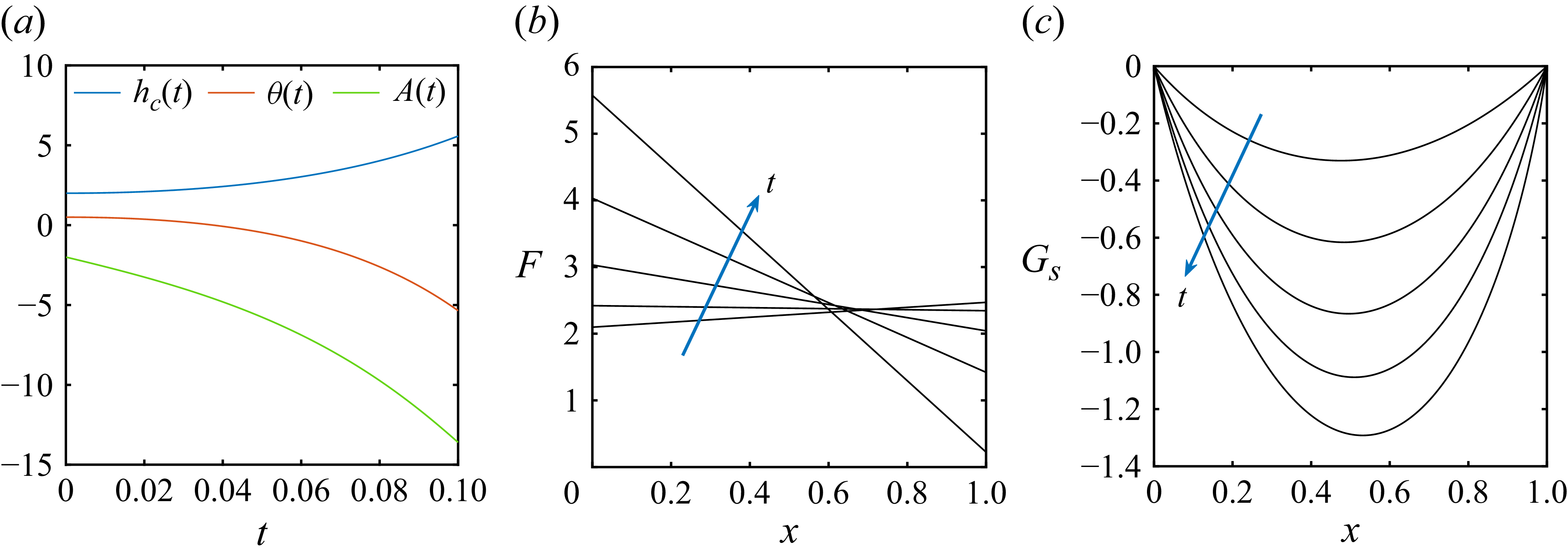


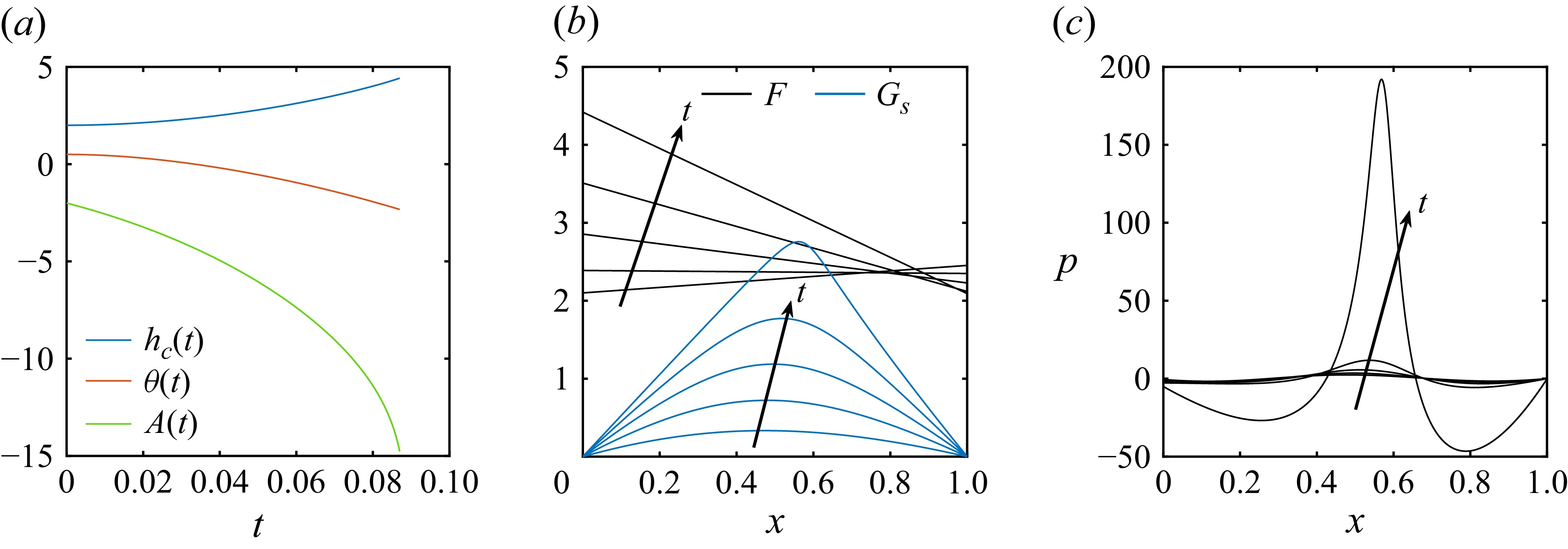


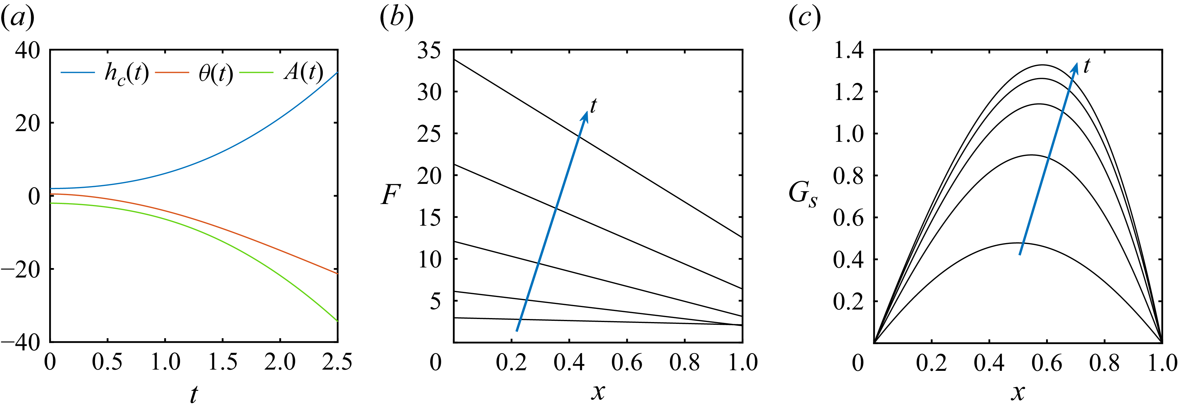


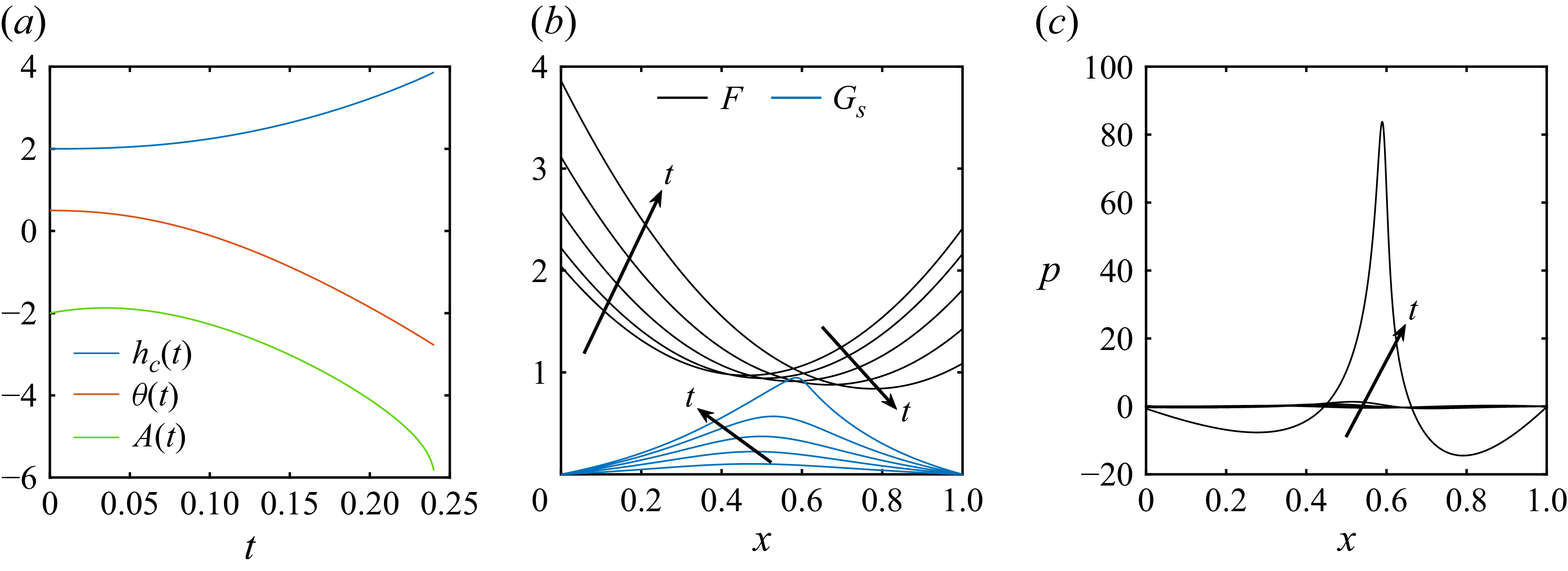


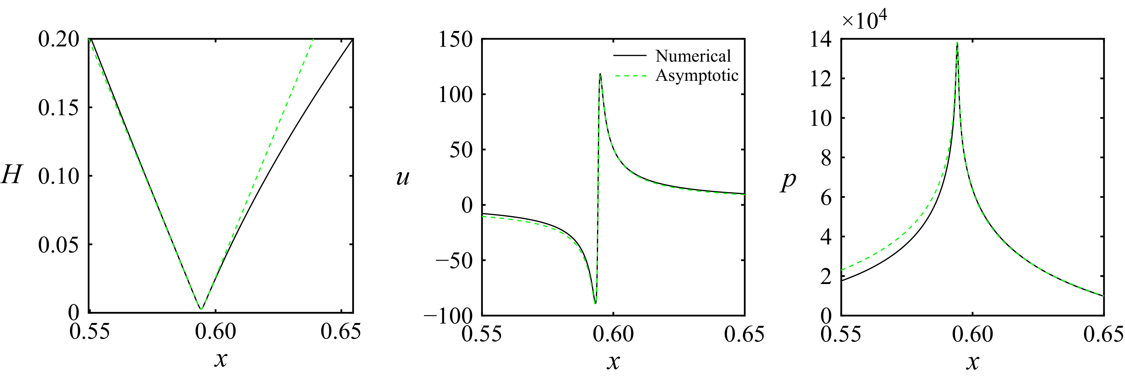


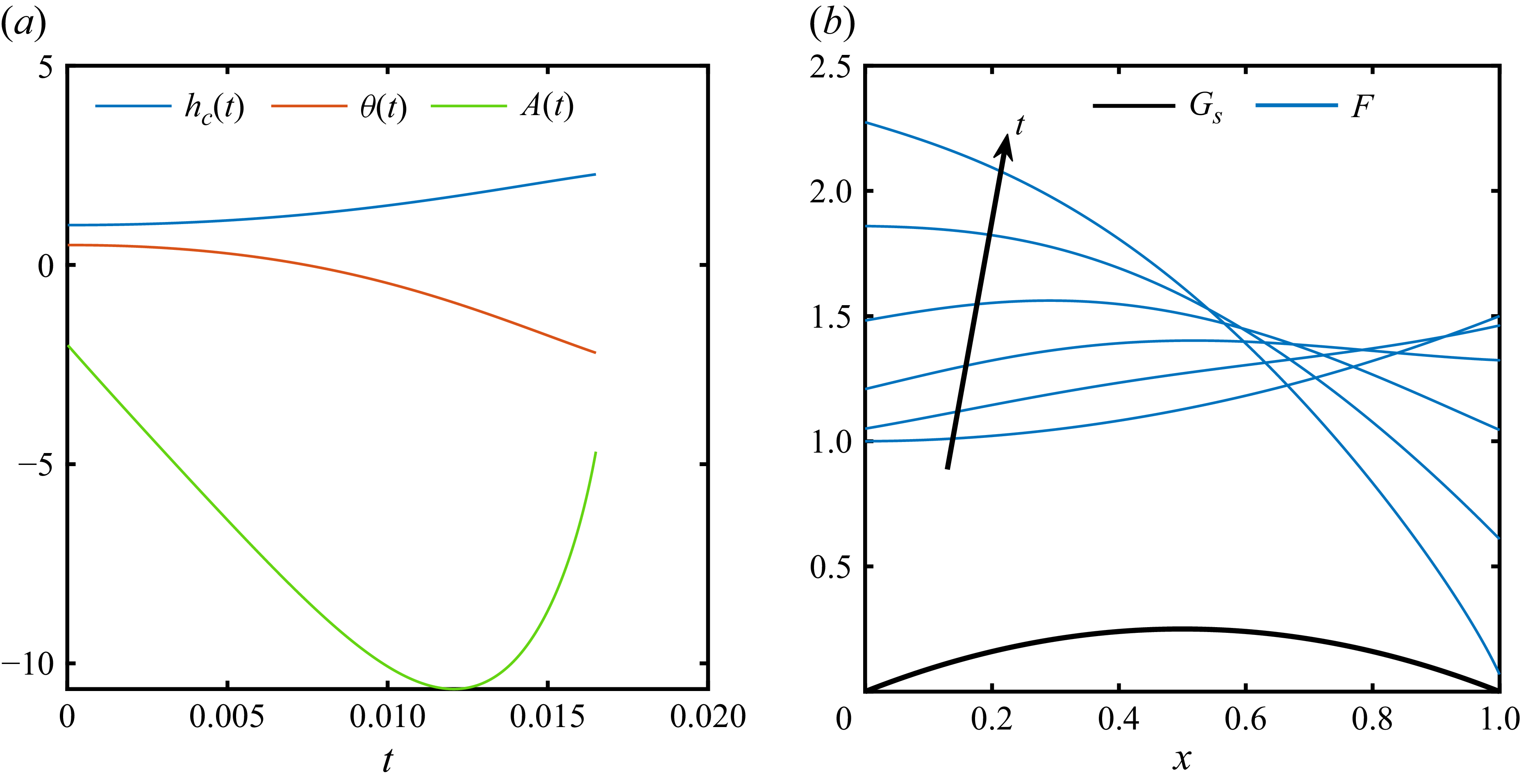


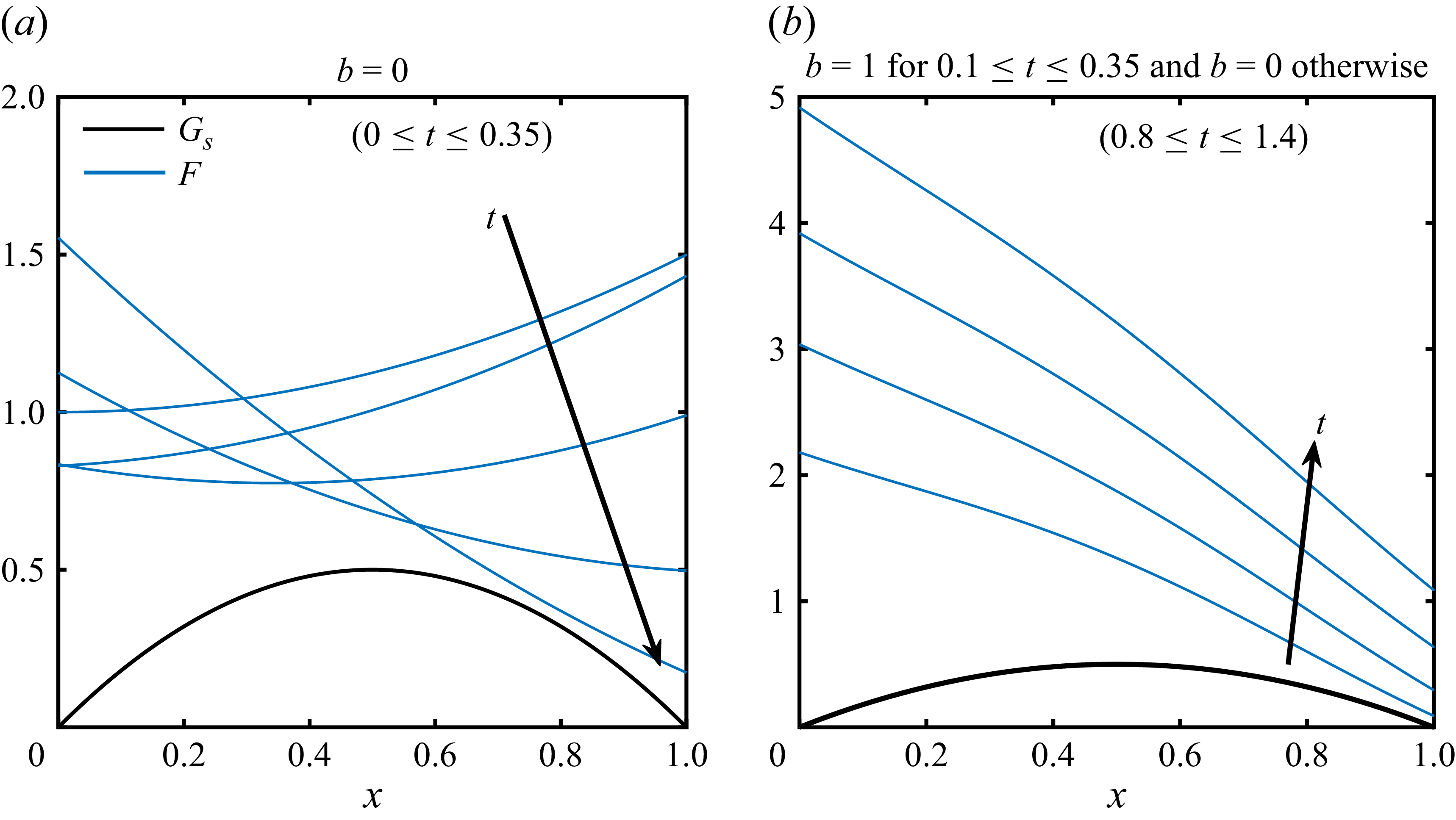


 Open access

